october 1975 hewlett-packard journal - hp labs · field and depot maintenance of radar and...

OCTOBER 1975

HEWLETT-PACKARD JOURNAL

W P - ' 1

'tuH

© Copr. 1949-1998 Hewlett-Packard Co.

Digi ta l Power Meter Offers Improved Accuracy, Hands-Off Operat ion, Systems Compat ib i l i ty This four -d ig i t genera l -purpose mic rowave power meter features autoranging, absolute or relat ive readings, 0.01 dB resolut ion, and 0.02 dB basic accuracy. Six power sensors cover a f requency range of 100 kHz to 18 GHz and a power r a n g e o f - 7 0 d B m t o + 3 5 d B m .

by A l len P . Edwards

BETTER DISPLAY RESOLUTION AND read ability and potentially easier interfacing with

other equipment for systems operation are the most immediate and obvious advantages of digital instru ments over their analog counterparts. Model 436A, a precision general-purpose digital power meter, brings these benefits and many others to the measure ment of RF and microwave power in a frequency range of 100 kHz to 18 GHz and a power range of -70 dBm to +35 dBm, depending on the power sensor be ing used. Automatic and remotely programmable, the new meter is an excellent instrument for general laboratory use, especially in the new calculator- controlled mini-systems based on the Hewlett-Pack ard Interface Bus (HP-IB). It is also well suited for pro duction testing, calibration, quality assurance, and field and depot maintenance of radar and transceiver systems.

Designed to be easy to use and interpret, Model 436A has a logically organized, uncluttered front panel, a large four-digit light-emitting-diode dis play, and an auxiliary analog meter for peaking ad justments (Fig. 1). Power readings can be displayed in absolute units of watts or dBm, or in dB relative to a previous input power level. This relative measure ment capability is useful for measuring parameters such as flatness and insertion loss, where absolute power levels are of no significance. Basic instrument accuracy, including sensor nonlinearity, is essen tially the same regardless of measurement units: Â±0.5% or Â±0.02 dB.

Model 436A measures power in five ranges, auto matically switching between ranges for hands-off operation. Autoranging can be disabled by means of a front-panel pushbutton.

The new meter accepts the 8481A, 8482A, and 8483A thermocouple power sensors,1'2 the high- power 8481H and 8482H, and the new Model 8484A

high-sensitivity low-barrier Schottky-diode power sensor (see article, page 8). The low SWR of these sensors â€” specified maximum SWR's are 1.1 to 1.3, depending on frequency â€” substantially reduces mis match uncertainty, the major source of error in micro wave power measurements. For example, with a sen sor SWR of 1.1 and a source SWR of 1.3, mismatch un certainty is a low Â±1.5%. The power meter automati cally recognizes which sensor is connected to it and

C o v e r : A m i n i - s y s t e m t h a t s h o w s o f f t h e f e a t u r e s a n d c a p a b i l i t i e s o f t h e n e w M o d e l 4 3 6 A D i g i t a l P o w e r M e t e r a n d t h e n e w M o d e l 8 4 8 4 A P o w e r S e n s o r ( f o r e g round) . A Hewle t t -Packard I n t e r f a c e B u s o p t i o n p u t s t h e 4 3 6 A u n d e r c a l c u l a t o r

con t ro l . The sensor a l lows accura te power mea s u r e m e n t s d o w n t o - 7 0 d B m .

In this Issue: Dig i ta l Power Mete r O f fe rs Improved Accu racy , Hands -O f f Ope ra t i on , Sys t e m s C o m p a t i b i l i t y , b y A l l e n P . E d w a r d s p a g e 2 V e r y - L o w - L e v e l M i c r o w a v e P o w e r Measurements , by Rona ld E . Pra t t . . page 8 A c t i v e P r o b e s I m p r o v e P r e c i s i o n o f T i m e I n t e r v a l M e a s u r e m e n t s , b y R o b e r t W . O f f e r m a n n , S t e v e n E . Schu l t z , and Char les R . T r imb le . . . . page 11 Flow Cont ro l in H igh-Pressure L iqu id Chromatography, by Helge Schrenker page 17

Printed in U.S.A. c Hewle t t -Packard Company , 1975


adjusts the displayed units and decimal point accord ingly.

An internal power calibrator provides an accu rate 50-MHz, 1-mW signal for matching the meter to any individual sensor. A manual front-panel GAL FAC TOR switch adjusts the meter for different sensor effi ciency values (supplied with each sensor]. A SENSOR ZERO button automatically zeros the meter and dis play.

Two remote-programming options are available, a binary-coded-decimal (BCD) arrangement and a more versatile HP-IB system. In the HP-IB system the power meter is both a listener and a talker, receiving commands and transmitting power readings over the bus. Both programming options are field-installable and the meter is easily converted from one to the other.

How I t Works The design of the 436A Power Meter is built on the

excellent base of the 435A Power Meter.2 The analog circuits of the two meters are very similar.

Fig. 2 is the block diagram of the 436A. The small dc voltage developed in the sensor is chopped into a 220-Hz square wave. This signal is then amplified and detected in synchronism with the chopping ac tion so that only 220-Hz signals of the proper phase contribute to the output.

In the 436A the synchronous detector was rede signed so that it rectifies the signal but does not filter it as the 43 5 A detector did. This was done so the de-

Fig. 1 . Model 436 A Dig i ta l Power M e t e r w i t h M o d e l 8 4 8 1 A P o w e r S e n s o r m e a s u r e s p o w e r f r o m 3 f i W t o 2 0 0 m W a t f r e q u e n c i e s from 10 MHz to 18 GHz. Five other sensors extend the f requency and power ranges.

lector would not limit the response time of the instru ment on the higher ranges. This change makes the 436A about four times faster than the 435A, a dif ference that becomes important when the meter is used in an automatic system.

Other minor changes were made to get somewhat better accuracy and temperature stability consistent with tighter specifications.

Logari thmic Analog-to-Digi ta l Converter The heart of this instrument is the logarithmic ana

log-to-digital converter (Fig. 3). This circuit, based on the standard dual slope conversion circuit, al lows readings in watts or dBm with the same accur acy and with a minimum of extra circuitry. Unlike analog approaches to the problem of log conversion, no warm-up time is required and there is very little temperature drift (<Â±.001 dB/Â°C).

At the start of a measurement cycle switch Sj closes and connects the unknown to the integrator ICl. After a fixed period of time T^ switch Sj opens. This has left a voltage V, on the integrator proportional to the unknown input voltage, which is proportional to input power. In the watts mode the appropriate refer ence voltage is then connected to the integrator us ing S2 or S3 until the comparator, IC2, detects a zero crossing. The discharge time, T2, is proportional to the unknown input and can be counted to get a digital result representing watts of input power. During T3 switches S6 and S7 are closed and a feedback loop is formed that puts a charge on C2 to remove the offset


Autozero Re turn

. Sensi t iv i ty

D e c o d e r A lgor i thmic

S t a t e M a c h i n e (ASM)

A- to-D Conver te r

R e m o t e I O Opt ion

â€¢â€¢

T i m i n g a n d C o u n t e r s

d B R e f e r e n c e S t o r a g e a n d

Counte rs

Fig. machine meter diagram of 436A Power Meter. Algorithmic state machine (ASM) automates meter operat ion, making i t very easy to use.

Output

Fig. dual- Logarithmic analog-to-digital converter uses the dual- s lope convers ion technique, g ives readings in wat ts or dBm. The c i r cu i t r equ i r es no wa rmup and has l i t t l e t empe ra tu re drift.

from ICl. R3 and C2 provide the dominant pole in the loop and R2 and C2 compensate for a pole in IC2.

If a log conversion is required, switches S4 and S5 are closed at the beginning of T2. This connects the output of the integrator back to the input. Thus the in tegrator output voltage is

V 0 = Vodt .

Solving this equation gives

T2 = log â€” . V2

Vj is the initial condition of the integrator; it is pro portional to the input voltage Vin, which is propor tional to input power P.

R,C,

V2 is a reference proportional to 0 dBm, or 1 mW. Then

n

T 2 = 1 0 l o g 1 mW

Ranging is accomplished by presetting the bottom- of-range dBm value into the counter at the beginning of T2 and counting from there.


Automatic Gain and Attenuation Measurements

The p rogrammab le fea tu res and low mismatch o f the 436A Power Meter and i ts assoc ia ted sensors a l lows ga in and loss measurements to be made a t hundreds o f f requenc ies in less t han one m inu te w i t h accu rac i es app roach ing Â±0 .6 dB . By us ing a second 436A Power Meter and a 1 1667A Power Sp l i t t e r , t he e f fec ts o f sou rce SWR can be d ramat i ca l l y reduced , improving typical accuracies to bet ter than Â±0.2 dB*.

Shown in the diagram is a system for making highly accurate measurements o f a t tenua t ion . The sys tem is capab le o f mea su r ing up to 50 dB o f a t tenua t ion , bu t i s bes t su i ted fo r mea surements of 30 dB or less.

9 8 3 0 A C a l c u l a t o r

9 8 6 6 A T h e r m a l P r in te r

1 0 6 3 1 A / B / C I n t e r f a c e C a b l e

436A ( O p t i o n 0 2 2 )

P o w e r M e t e r 2

8481 A P o w e r

S e n s o r

4 3 6 A ( O p t i o n 0 2 2 )

P o w e r M e t e r 1

8481 A P o w e r

S e n s o r

8 6 6 0 A C ( O p t i o n 0 0 5 ) S y n t h e s i z e d

S i g n a l G e n e r a t o r

This is a very accura te measurement techn ique because a l most a l l major errors, except mismatch, can be cal ibrated out . Typical mismatch uncertainties are between Â±0.1 and Â±0.2 dB. Inst rumentat ion wi l l typ ica l ly add Â±0.02 dB to the tota l er ror . On the top range only, sensor nonl inear i ty adds Â±0.06 dB.

A l though th i s techn ique i s bes t su i ted fo r a t tenua t ion mea s u r e m e n t s o f 3 0 d B o r l e s s , m e a s u r e m e n t s o f a t t e n u a t i o n l e v e l s f r o m 3 0 t o 7 0 d B c a n b e m a d e u s i n g t h e 8 4 8 4 A H i g h S e n s i t i v i t y P o w e r S e n s o r . T h e s e t - u p i s t h e s a m e , e x c e p t tha t the 8484A Power Sensor i s connec ted to power mete r 1 in the diagram.

For cont inuous measurements of at tenuat ion f rom 0 to 70 dB ( f o r m a y f o r s w e e p t e s t i n g f i l t e r s ) , t h e t e s t c h a n n e l m a y b e modif ied so that i t contains a switch and two power meters, one wi th an 8481 A Sensor and one wi th an 8484A Sensor . Dur ing t h e m e a s u r e m e n t p h a s e o f t h e c y c l e , t h e 8 4 8 4 A S e n s o r i s s w i t c h e d i n t o t h e c i r c u i t w h e n t h e p o w e r f a l l s b e l o w a b o u t - 2 5 d B m a n d t h e 8 4 8 1 A S e n s o r i s s w i t c h e d i n t o t h e c i r cu i t when the power goes above app rox ima te l y - 21 dBm.

HP App l i ca t ion Note 196 g ives de ta i l s o f measurement p ro cedures and 9830A Calculator programs, and presents several o ther min i -system appl icat ions of the 436A. ' F o r a d i s c u s s i o n o n t h e u s e o f a p o w e r s p l i t t e r t o r e d u c e s o u r c e S W R . s e e H e w l e t t - P a c k a r d A p p l i c a t i o n N o t e 1 8 3 . " H i g h F r e q u e n c y S w e p t M e a s u r e m e n t s . ' A p p e n d i x A .

Algor i thmic State Machine The decision to use a specially designed analog-to-

digital converter instead of a panel meter led us to choose a ROM-programmed algorithmic state machine as a controller for the instrument. The benefit is that such a machine can do much more than sequence the A-to-D converter, with little additional hardware or cost. The approach is also sufficiently flexible that several fine points are included that would normally be left out for economy in a discrete logic design. For example, there is an under-range light to tell the user when the meter is not on the optimum range (if range hold is in use). In watts mode the under-range point is 10% of full scale. If the machine is on the bottom range, even when the reading is less than 10% of full scale there is no better range and the light does not go on. If the instrument is in dBm mode the light goes on if the reading is less than 10 dB below full scale. All of this decoding is in firmware (ROM) and the only hardware associated with the light is a latch- driver. This coding arrangement may not seem im portant, but it is an example of making use of firm ware to improve the usability of the instrument by minimizing confusion. Some of these changes were made in the course of development with only pro gramming changes, further evidence that instrument behavior is a matter of choice with state machine de sign and no longer an engineering trade-off.

As an example of one firmware routine in the state machine program, consider the control routine for the relative-dB circuit (Fig. 4). This circuit takes the ratio of two power levels by storing the reference power in dBm and subtracting it from the measured power, also in dBm. The subtraction is done in two tracking counters. The timing counter contains a count equal to the dBm input power P. This counter is counted down until the synchronous counter that contained the reference quantity R reaches zero. At this point the timing counter contains

lOlog P-10log R = IOlog P/R.

A study of the flow graph shows how the state ma chine exercises a relatively small amount of hard ware to do this job. Note that because counting stops when the relative counter underflows (= -1) this gives one too many counts. To compensate, an extra count is initially clocked into this counter so the underflow represents zero.

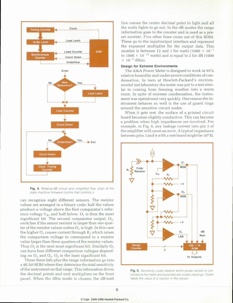
Sensit ivi ty Coder The sensitivity coder, Fig. 5, is responsible for the

instrument's ability to know which sensor is con nected to it and to scale all readings appropriately. This circuit makes use of a simple A-to-D converter and a 4K ROM. The A-to-D converter reads the value of a coding resistor in the sensor. The circuit uses three comparators to generate eight codes; thus it


Clock

Load Counter

Exit

F ig . 4 . Re la t i ve -dB c i r cu i t and s imp l i f i ed f l ow cha r t o f t he state machine f i rmware rout ine that contro ls i t .

can recognize eight different sensors. The resistor values are arranged in a binary code; half the values produce a voltage above the first comparator's refer ence voltage VR1 and half below. Oj is then the most significant bit. The second comparator output, O2, switches if the sensor resistor is larger than one quar ter of the resistor values unless Ol is high. In this case the higher Ot causes current through R2 which raises the comparison voltage to correspond to a resistor value larger than three quarters of the resistor values. Thus O2 is the next most significant bit. Similarly O3 can have four different comparison voltages depend ing on Oj and O2. O3 is the least significant bit.

These three bits plus the range information go into a 4K-bit ROM where they determine the total sensitivity of the instrument on that range. This information drives the decimal points and unit multipliers on the front panel. When the dBm mode is chosen, the dB/watt

line causes the center decimal point to light and all the watts lights to go out. In the dB modes the range information goes to the counter and is used as a pre set number. Five other lines come out of this ROM. These go to the input/output interface and represent the exponent multiplier for the output data. This number is between 12 and 1 for watts (1000 x 10"1 to 1000 x 10~12 watts) and is equal to 2 for dB (1000 x 10~2 dBm).

Design for Extreme Environments The 436A Power Meter is designed to work in 95%

relative humidity and under severe conditions of con densation. In tests at Hewlett-Packard's environ mental test laboratory the meter was put to a test simi lar to corning from freezing weather into a warm room. In spite of extreme condensation, the instru ment was operational very quickly. One reason the in strument behaves so well is the use of guard rings around the sensitive circuit nodes.

When it gets wet, the surface of a printed circuit board becomes slightly conductive. This can become a problem when high impedances are involved. For example, in Fig. 6, any leakage current into pin 3 of the amplifier will cause an error. A typical impedance between pins 3 and 4 with a wet board might be 109 fi,

Range Counter

256 x 16 ROM

16 Outputs

Fig . 5 . Sens i t i v i t y coder de tec ts wh ich power sensor i s con nected to the meter and automatical ly scales readings. Coder reads the value of a res is tor in the sensor.


Guard Trace

F ig . 6 . Guarded amp l i f i e r i npu ts reduce l eakage p rob lems w i t h w e t p r i n t e d c i r c u i t b o a r d s , m a k i n g i t p o s s i b l e l o r t h e 436A to work in 95% re la t ive humid i ty and under severe con di t ions of condensat ion.

allowing enough current to flow into pin 3 to cause an error voltage of 2.25 mV, which would make the instrument go out of specification.

With the help of computer printed circuit layout, guard traces have been placed around amplifier input terminals inthe436A (A and B in Fig. 6). These traces are connected to a low-impedance node (C in Fig. 6), so any current flowing toward the input terminals will flow into the guard ring and be grounded through the low-impedance node without develop ing an error voltage.

Acknowledgments I would like to thank Bob Waldron for the excellent

mechanical design evident in the simplicity of the final product, Cory Boyan for his design of the BCD

mi Al len P . Edwards Al len Edwards was pro ject leader

^ f o r t h e 4 3 6 A P o w e r M e t e r . H e L " J r ^ ^ ^ T " ^ ^ _ r e c e i v e d h i s B S a n d M S d e g r e e s â€” â€” â€” â€¢â€” " â€¢**â€¢â€¢ I in electrical engineering from

Stanford Univers i ty in 1971 and jo ined HP the same year . He has cont r ibuted to the des ign of the 8558B Spect rum Ana lyzer and the 435A Power Meter and holds a pa ten t on the logar i thmic conver ter in the 436A. Al len was born and ra ised in Los Angeles . He 's married and now lives in Palo Alto, Cal i fornia. A cycl ing enthusiast , last year he b icyc led f rom Palo

Al to to in Angeles, a 450-mi le, s ix-day t r ip. He also dabbles in photography and enjoys backpacking. He's a member of IEEE.

interface, and Roger Graeber for his attention to de tails that made for such a smooth introduction of this product.Â»

References 1. W.H. Jackson, "A Thin-Film/Semiconductor Thermo couple for Microwave Power Measurements," Hewlett- Packard Journal, September 1974. 2. J.C. Lamy, "Microelectronics Enhances Thermocouple Power Measurements," Hewlett-Packard Journal, Sep tember 1974.

S P E C I F I C A T I O N S HP Model 436A Dig i ta l Power Meter

FREQUENCY RANGE: 100 kHz to 18 GHz (depend ing on power sensor used) . P O W E R R A N G E :

WITH of A , 8482A, OR 8483A SENSORS: 50 dB wi th 5 fu l l sca le ranges o f 10 and 100/ jW; 1, 10 and 100 mW. The display is a lso cal ibrated in dBm and dB f rom -20 dBm to +20 dBm fu l l sca le i n 10 -dB s teps .

WITH ranges A-H01 OR 8482A-H01 SENSORS: 45 dB with 5 full-scale ranges of 1 , 10 and 100 mW: 1 and 3 wat ts. The display is a lso cal ibrated in dBm and dB from 0 from to Â»30 dBm ful l scale in 10-dB steps, and a 5-dB step from -1-30 d B m t o * 3 5 d B m .

I N S T R U M E N T A T I O N A C C U R A C Y ' : WATT MODE: Â±0.5% in ranges 1 through 4: Â±1.0% in range 5. D B M M O D E : Â ± 0 . 0 2 d B Â ± 0 . 0 0 1 d B / Â ° C i n r a n g e 1 t h r o u g h 4 ; Â ± 0 . 0 4 d B

Â±0.001 dB/Â°C in range 5. DB(REL) MODE2: Â±0.02 dB Â±0.001 dB/Â°C in ranges 1 through 4; Â±0.04 dB

+ 0.001 dB'Â°C in range 5. ZERO: automat ic , operated by a f ront -panel swi tch ZEROSET: Â±0.5% of full scale on most sensit ive range, typical. Â±1 count on other

ranges. ZERO CARRY OVER: -0.2% of ful l scale when zeroed on the most sensit ive range NOISE: peak-to- 8481A, 8482A and 8483A sensors; Â±0.5% of fu l l scale peak-to-

peak on the most sensi t ive range typ ical . Less in h igher ranges. LONG TERM ZERO DRIFT (8 h rs ) : Â±2% o f fu l l sca le on mos t sens i t i ve range

( typical at constant temperature). RESPONSE TIME: (0 to 99% o f read ing) w i th 8481A, 8482A, 8483A sensors ;

RANGE 1 - 10 seconds (most sens i t i ve range) R A N G E 2 < 1 s e c o n d RANGE 3 t h rough 5 <100 msec (Typical , measured at recorder output) .

REFERENCE OSCILLATOR: In te rna l 50 MHz osc i l l a to r w i th Type N fema le con nector mW. f ront panel or rear panel (Opt ion 003 only) . Power output 1 .0 mW. Factory set to Â±0.7% traceable to the National Bureau of Standards. Accuracy: Â±1.2% worst case (Â±0.9% rms) for one year (0CC to 55Â°C).

CAL FACTOR: 16 -pos i t i on sw i t ch no rma l i zes mete r read ing to accoun t fo r ca l i brat ion factor . Range 85% to 100% in 1% steps.

CAL ADJUSTMENT: Front -panel ad jus tment prov ides capabi l i ty to ad jus t ga in in meter to match power sensor in use.

RECORDER OUTPUT: Propor t iona l to ind icated power wi th 1 vo l t cor responding to fu l l sca le and 0.3I6 vo l ts to -5 dB; 1 k i i output impedance, BNC connector .

RF BLANKING: Open co l lec tor TTL; low cor responds to b lank ing . DISPLAY: Digi ta l d isplay wi th four d ig i ts . 20% overrange capabi l i ty on al l ranges.

Analog Meter : uncal ibrated peaking meter to see fast changes. POWER: wat ts 120. 220, o r 240 V +5%, -10%. 48 to 440 Hz. less than 20 wat ts

( less than 23 wi th d ig i ta l inputoutput) . WEIGHT: Net . 4 .5 kg (10 Ib) . PRICES IN U.S.A. : 436A Power Meter . S1800.

3m (10 f t ) cab le for power sensor . $10 6.1 m (20 f t ) cable for power sensor , $55 15.2 m (50 f t ) cable for power sensor . $105 30.5 m (100 f t ) cable for power sensor . $155 61 m (200 f t ) cab le for power sensor . $260 Dig i ta l inputoutput . fu l ly compat ib le wi th HP Inter face Bus (HP-IB) . $375 Dig i ta l inputoutput fu l ly compat ib le wi th BCD Inter face. $275

M A N U F A C T U R I N G D I V I S I O N : S T A N F O R D P A R K D I V I S I O N 1501 Page Mi l l Road Palo Al to, Cal i forn ia 94304 U.S.A.

i n c l u d e s a n y s e n s o r n o n l i n e a r i t y . 2 S p e d f i c a t i o n s a r e f o r w i t h i n r a n g e m e a s u r e m e n t s . F o r r a n g e - t o - r a n g e a c c u r a c y a d d t he r ange unce r t a i n t i es


Very-Low-Leve l Microwave Power Measurements A new low-bar r ie r Scho t tky d iode power sensor makes i t poss ib le to measure power as low as 100 p icowat ts over a f requency range o f 10 MHz to 18 GHz.

by Ronald E . Prat t

ANEW POWER SENSOR, MODEL 8484A, has been developed for measuring microwave

power levels down to 100 picowatts overa frequency range of 10 MHz to 18 GHz. It is compatible with any 435A or 436A Power Meter, and its power range is -20 to -70 dBm, a range that begins where most other sensors become noisy or subject to thermal drift. Higher power levels up to +35 dBm can be measured with other sensors,1 so with one meter and three sen sors, a 105-dB measurement range is possible.

Like its predecessors, the 8484A (Fig. 1) has a low SWR specification:

1.15 30 MHz to 4 GHz 1.2 4 GHz to 10 GHz 1.3 10 GHz to 18 GHz.

Low sensor SWR minimizes measurement error caused by multiple mismatch interaction between the sensor and the source being measured. Typically, this interaction is the major source of error in a power measurement.

The power sensing element in the 8484A is a diode detector. For peak power levels up to â€”20 dBm, the diode is a square law device so it yields a true indica tion of power, independent of the waveform of the signal being measured. As the peak power is in creased above -20 dBm, the diode response changes from square law to linear, so it becomes sensitive to signal waveform. With a peak power of +10 dBm, as much as 2 dB of error has been observed when mea suring signals with amplitude modulation or high harmonic content. For this reason, the maximum power specification of the 8484A is -20 dBm, a level below which waveform-related errors are negligible.

Burnout of the power sensor is always a user con cern. The 8484A detector diode can withstand 200 milliwatts ( + 23 dBm), so the user has a safety margin of 2X104 in power.

The diode detector in the 8484A is a newly devel

oped low-barrier Schottky diode. A thin-film match ing circuit provides a 50-ohm termination. The diode and matching circuit are described elsewhere in the literature.2 The RF voltage across the 50-ohm load is rectified by the diode, following the square law, and the resulting dc voltage is measured and displayed by the power meter. This rectification is about 5 xlO3 more efficient than the RF-to-dc conversion of the higher-power thermocouple sensors. The small sig nal gain of the amplifier built into the sensor is doubled to adjust the scale factor so that decade power ranges are maintained.

The power meters were designed with a shaping network to compensate for the high-power nonlinearity inherent in a thermocouple. Another shaping network in the 8484A makes the amplifier output match this nonlinearity. In this way, the accuracy specification of the meter-sensor combination is not degraded.

The output voltage of the detector is about 50 nano-

Fig . 1 . Mode l 8484A Power Sensor works w i th HP 435A and 436A Power Mete rs to measure power f rom -70 to -20 dBm o v e r a f r e q u e n c y r a n g e o f 1 0 M H z t o 1 8 G H z . C a l i b r a t i o n fac tor is shown on hous ing as a funct ion o f f requency.

8


Matching Network

Regions of High Thermal Conduct iv i ty

Regions of Low Thermal Conduct iv i ty

Fig. drawing acts housing is designed for low thermal drif t . In the drawing the housing A acts as a sink for heat from the RF connector or as a source for heat caused by handl ing. Low-conductivi ty reg ion B which heat to one end of the d iode module , and to h igh-conduct iv i ty reg ion C, which transfers it to the opposite end of the module. High-conductivity region D distributes the heat from B and with uniformly. Region E balances the heat transfer from C to D with that from BtoD. Reg/on F b locks d iode t ransfer f rom c i rcu i t housing G. The photo is an in ter ior v iew of the d iode module showing gradient diode chip, the matching network, and the region where a temperature gradient

Af w i l l genera te a thermal EMF.

volts dc with an applied power of -70 dBm. Circuit layout had to be handled very carefully to prevent leakage signals or extraneous thermoelectric vol tages from swamping out the desired signal. The FET chopper used in the thermocouple sensors was re designed for the diode sensor to allow separation of autozero and signal paths, and a marked improve ment in thermal stability was obtained by using an integrated circuit approach.

Thermal drift is always encountered in the mea surement of low power levels. For the 8484A, drift becomes noticeable below 1 nanowatt. The major drift mechanism is a thermal EMF generated by a temperature gradient that appears across the diode. The mechanical design of the 8484A minimizes this gradient by insulating the diode package and arrang ing the thermal paths so the primary heat source is at the RF input connector. Any heat that does enter the diode area is directed uniformly to both ends of the diode package. With both ends changing tempera ture uniformly, the temperature gradient across the diode remains almost constant, thus minimizing drift. Thermal drift is further reduced by the heat sinking ac tion of an aluminum extrusion which forms the outer housing of the 8484A. Details of the thermal design

are shown in Fig. 2. Fig. 3 compares the drift of an 8484A with that of a typical thermistor sensor. The heat source was a warm hand and both sensors were in their most sensitive ranges. Note that there is a

F ig . 3 . D r i f t o f a t yp i ca l 8484A H igh -Sens i t i v i t y Power Sen sor in response to a hand grasp, compared wi th that of a typi cal thermistor power sensor. Both sensors were on their most sensi t ive ranges, which di f fer by 104 in sensi t iv i ty .

9


factor of 104 difference in scale factor. Higher power ranges are of course almost drift free.

Each 8484A is supplied with an individual calibra tion factor curve as well as a more precise tabular da ta sheet. This calibration information is measured us ing a modified 8542B Automatic Network Analyzer. Unlike bolometric or thermoelectric power sensors, the efficiency of the diode detector is not always a maximum at the low RF frequencies. Since effi ciency 17 and calibration factor are related by:

C.F. = T, (1-p2)

where p is the magnitude of the sensor's reflection coefficient, the calibration factor could exceed 100% if it were always referenced to 100% at 50 MHz. The program used to calibrate the 8484A normalizes the calibration factor to the frequency where the diode is most sensitive. When the calibration factor label is printed, the computer writes the correct 50-MHz cali bration factor on the label. The normalization is per formed such that an integer always results (the CAL FACTOR switch on the power meter has integer steps).

The CAL FACTOR switch must be placed on the ap propriate setting when the CAL ADJUST control is be ing set. A special reference attenuator, the 11708A, reduces the meter's reference oscillator power to one microwatt to allow calibration of the 8484A. This attenuator is accurate and well matched, so a maxi mum of 1% error is added to the calibration step.

The sensitivity of the diode detector in the 8484A is influenced by ambient temperature. This change has been compensated for, but at extreme ambient temperatures, the instrument should be recalibrated using the reference oscillator and the 11 708 A to ob tain the most accurate results. Typical temperature- sensitivity variations for uncompensated and com pensated detectors are shown in Fig. 4.

The 8484A is fully compatible with all 435A and 436A power meters. The 436A offers digital display

Uncompensated Diode

2 0 3 0 Temperature ( C)

4 0 5 0

Fig. 4. Typical sensi t iv i ty var iat ions with ambient temperature f o r c o m p e n s a t e d ( 8 4 8 4 A ) a n d u n c o m p e n s a t e d d i o d e s e n sors. Reca/ ibrat ion is recommended at extreme temperatures for most accurate resul ts.

and many other user conveniences. On its most sensi tive range, the 8484A is noisier than the other sen sors, so the more effective filtering found in the 436A is an advantage when measuring 100 picowatts to 1 nanowatt.

Acknowledgments Many people contributed to the 8484A project.

Special thanks go to Brent Palmer for guidance in the early phases of the project, Pete Szente for supplying an excellent detector design, and Les Brubaker for picking up the difficult final design of the amplifier shaper circuit. Bob Kirkpatrick was responsible for the 11708A. Industrial design was by Yas Matsui.E

References 1. J.C. Lamy, "Microelectronics Enhances Thermocouple Power Measurements," Hewlett-Packard Journal, Sep tember 1974. 2. P. A. Szente, S. Adam, and R.B. Riley, "Low-Barrier Schottky Diode Detectors," to be published.

Ronald E. Prat t Ron Pra t t has been des ign ing m ic rowave componen ts fo r sweepers, network analyzers, and power mete rs s ince he came to HP in 1967; h is la tes t

- - ^ | _ i s t h e 8 4 8 4 A P o w e r S e n s o r , ; â € ¢ Â « â € ¢ â € ¢ A 1 9 6 7 B S E E 9 r a d u a t e o f

â € ¢ N e w a r k C o l l e g e o f E n g i n e e r i n g , | Â ¿ Â £ ^ d Ã I h e ' s a m e m b e r o f I E E E a n d

has t augh t m i c rowave e l ec t ronics at Foothi l l Col lege for s ix years . Ron was born in Buf fa lo , New York and now l ives in San Jose. Cal i fornia. He 's marr ied, has two smal l

daughters, and enjoys cabinet making and t inker ing wi th cars.

S P E C I F I C A T I O N S HP Model 8484A Power Sensor

FREQUENCY RANGE: 10 MHz -18 GHz POWER RANGE: 100 pW-10 /xW SWR (REFLECTION COEFFIC IENT) : <1 .40 (0 .167 ) 10 -30 MHz; <1 .15 (0 .070 )

30 MHz -4 GHz ; ' 1 . 20 (0 .091 ) 4 -10 GHz ; <1 .30 (0 .130 ) 10 -18 GHz M A X . A V E R A G E P O W E R : 2 0 0 m W M A X . P E A K P O W E R : 2 0 0 m W NOMINAL IMPEDANCE: 50Ã1 RF CONNECTOR: Type N Male PRICE IN U.S.A.: S550

OPT ION 002 Range knob w new sca le mark ings fo r 435A Ser No . 1530A and below: $25

O P T I O N t o D e l e t e 1 1 7 0 8 A 3 0 - d B c a l i b r a t i o n p a d ( 1 1 7 0 8 A i s f a c t o r y s e t t o Â±0.05dB at 50 MHz. traceable to NBS, SWR <1.05): less S50

M A N U FA C TU R IN G D IV IS ION : STA N FOR D PA R K D IV IS ION 1501 Page Mill Road Palo Alto. California 94304

10


Act ive Probes Improve Precis ion of T ime Interval Measurements Usable wi th most t ime in terva l counters , th is new probe sys tem he lps so lve p rob lems caused by t r igger po in t inde terminacy , sys tem de lay er ro rs , inadequate dynamic range, and c i rcu i t loading.

by Robert W. Offermann, Steven E. Schultz, and Charles R. Trimble

IN ELECTRONICS, A TIME INTERVAL is the dif ference between the times of occurrence of two

electronic events, usually points on a voltage wave form. Time interval measurement is normally done with oscilloscopes or with electronic counters that have time interval measuring ability. However, even the best oscilloscopes and counters have certain limitations in time interval measurements.1

It is these shortcomings that the new Model 5363A Time Interval Probes (Fig. 1) are designed to over come. The probes optimize input signals for a coun ter's front end. Their contribution is best understood by considering the problems they are designed to solve.

Oscilloscopes Oscilloscopes display a waveform in its entirety,

allowing the user to see an amplitude-versus-time plot of the signal. To use an oscilloscope to measure time interval, the user must locate the desired start and stop points on the displayed waveform and then read the time interval from the time axis. The main problem with most oscilloscopes is that neither the voltage axis nor the time axis is precise. In high- frequency time interval measurements using sam pling scopes or active-probe real-time scopes, dynamic range limitations may cause even greater errors because imprecise voltage dividers are often needed. The latest oscilloscopes, such as the HP Model 1722A with its built-in digital processor,2 overcome these limitations to a great extent, achiev ing accuracies as great as 0.6% for longer time inter vals. However, time base calibration is required every

F i g . 1 . M o d e l 5 3 6 3 A T i m e I n t e r v a l P r o b e s c o n s i s t o f t w o l o w - capaci tance (10pF) act ive probes a n d a s s o c i a t e d e l e c t r o n i c s i n a separate box. Ei ther probe can be u s e d a l o n e t o m a k e s t a r t / s t o p m e a s u r e m e n t s o r b o t h p r o b e s can be used, one for start and one for s top. Tr igger leve ls are adjust ab le f rom -9 .99 V to +9 .99 V . An a d j u s t a b l e d e l a y e q u a l i z e s p r o p a g a t i o n t i m e d i f f e r e n c e s i n s tar t and s top channels .

11


few hours to maintain accuracy, and time intervals must be repetitive to allow the operator to set up the measurement. The latter requirement makes it dif ficult to measure single-shot intervals and jitter. Also, because a human operator must set and read the time interval from a CRT screen, or in the case of the newer scopes from a processor display, oscilloscopes in general are not suitable for systems applications in which digital programming and digital output are desired.

Counters Digital counters that have time interval capability

are potentially more accurate than oscilloscopes in the time domain because they provide a precise time base for measurements of time interval. The biggest problem that counters have in time interval mea surement is that their input circuits are optimized for frequency counting, that is, for detecting zero cross ings. Because of this, setting the trigger levels that define the limits of time intervals is difficult. The trigger level setting usually has a limited range, typi cally Â±1 volt or less, and its position can only be known accurately by using a digital voltmeter built into the counter or connected externally. At best,

Actual Tr igger Points

Selected Tr igger

Level VH

Hysteresis Band (May Vary wi th Input

Signal Rise Time)

(a ) Hysteres is Prob lem of Typ ica l Counter

System Triggers

First Threshold Passes 0V

(b ) 5363A Automat ic Ca l ib ra t ion Scheme El iminates Hysteresis

Fig . 2 . (a ) Because o f hys te res is , the ac tua l t r igger po in t o l a c o u n t e r i s o f f s e t f r o m t h e s e l e c t e d l e v e l b y a n u n k n o w n amoun t , o f t en 50 mV o r so . (b ) Mode l 5363 /4 T ime In te rva l P robes au tomat i ca l l y ca l i b ra te themse lves : t hey de tec t t he a c t u a l r e f e r e n c e v o l t a g e a t w h i c h a g r o u n d e d p r o b e t r i g g e r s , t h e n a d d t h i s o f f s e t t o t h e r e f e r e n c e v o l t a g e i n s u b sequent measurements . Ac tua l t r igger leve l i s then w i th in a few mi l l ivo l ts of the selected level .

however, this trigger level setting is the center of the hysteresis band of the counter input (Fig. 2); at worst, it is offset from this center in an unspecified manner by several tens of millivolts. Therefore, the actual triggering point of the input amplifier will be offset from the selected or measured level by an unknown amount. Furthermore, this offset may be different de pending upon which slope the counter is triggering on, and it can also change with the input frequency and signal level. The result is that one seldom knows the actual trigger point of a counter to better than 50 mV, and the ambiguity is often much greater. Because of the limited dynamic range of counters, dividers must be used to measure larger signals. This only increases the trigger level ambiguity problem.

Some counters use hysteresis compensation to give a more usable indication of the actual trigger voltage. Here an approximation of one-half the hysteresis band is added to (positive slope) or subtracted from (negative slope) the selected trigger level or reference voltage. Such compensation does not eliminate the hysteresis window, but it does make counters with a large window more usable.

The other limitation of a counter input amplifier is that it provides either a 50Ã1 termination or a high input resistance with a rather large shunt capaci tance, typically about 30 pF. This limitation makes it difficult to transport the signal to the counter without impedance transformation or distortion caused by the shunt input capacitance.

Counters have two other subtle problems. First, start and stop channels of counters often have dif ferent propagation delays, and these must be compen sated for precision time interval measurement. Sec ond, the propagation delay through a counter input amplifier is a function of the amount that the input signal goes past the trigger level, so careful under standing of the behavior of counters is necessary for accurate use of a counter in measuring precision time intervals.

Because counters are basically digital, they have been the workhorses in systems for measuring time intervals. Many have programmable front ends, and can select trigger levels and output the results via digital interfaces such as the HP Interface Bus (HP-IB). Of course, the programmable counter suffers from the same trigger level accuracy and signal condi tioning problems as the manual counter.

Time Interval Probes The 5363A Time Interval Probes consist of two

low-capacitance active probes and associated elec tronics in a separate box. Any universal electronic counter can be used with the probes, but to get the full benefit of the system, the counter should have input amplifiers that have at least 100 MHz bandwidth and

12


at least 10 nanoseconds resolution when measuring single-shot events. True time interval averaging is desirable.

The probes solve the problem of trigger level inde terminacy by an automatic calibration scheme (see Fig. 2) instead of hysteresis compensation. The user grounds the probe to be calibrated and presses a front panel switch. This causes the reference voltage, VR in Fig. 2, to move down in a stair-step fashion (up for negative slope calibration) in 1-mV steps until the de vice just triggers at zero volts. Knowing the value of VR at this point allows the system to adjust itself so the actual trigger voltage corresponds to the trigger level selected by the user. Recalibration when slopes or probes are changed assures constant triggering accuracy.

Any trigger voltage from -9.99 volts to +9.99 volts may be set in 10-millivolt steps manually by setting two front-panel thumbwheel switches. Remote set ting of the trigger voltage is also possible.

The probes' 20-volt dynamic range and precise trig

ger-point determination eliminate the need for atten uators in most cases and allow measurements closer to the top and bottom of the waveform than was pre viously possible.

Circuit loading caused by shunt capacitance is minimized by the probes' small 10 pF input capaci tance. Input resistance is 1 Mil.

The problem of propagation delay differences in the start and stop channels is solved by an adjustable delay in the stop channel, which can be used to com pensate for delay differences as large as two nano seconds. When a counter that has a minimum time in terval limitation is used, a fixed ten-nanosecond de lay can be switched in to allow measurements down to zero time.

For automated waveform analysis, such as in pro duction testing, the probes can be controlled re motely, for example by a desk-top calculator. Option Oil adds the programming ability of the calculator and HP-IB to the probes.

Start Reference

Outputs to Counter

Start

Stop

Stop Trigger Level Output

Start Trigger Level Output

Auto Calibration Circuits

D-to-A Converter

Fig. green above probe has a potential start and stop input. Red and green trigger lights above each probe indicate which probe has been selected for stop and start , respect ively, and f lash off when

t r igger ing occurs . A s ta te mach ine cont ro ls sys tem opera t ion .

13


Slope Select Output

to Counter

Probe Input > â € ” * * A V V n

-v

A Probe

Fig. The presents or stop channel is basically a voltage comparator. The input circuit presents a stan dard comparator wi th a s ignal that has a s ing le t rans i t ion d i rect ion and a smal l dynamic range

centered in the compara tor 's w indow.

P r o b e D e s i g n The 5363A Time Interval Probes are designed to en

hance the accuracy of time interval counters by pro viding signal conditioning and precision voltage references for the counters' front ends. The probes' outputs are fast-zero-crossing signals for which a counter's front end is optimized. The probes are sim ple to understand and use, fully programmable, and rack mountable for systems use.

As the block diagram, Fig. 3, shows, the 5363A has two active probes, each with a potential start and stop input. Either probe can be used alone to measure a rise time, for example, or used with the other probe to measure a time delay between two separate sig nals. Probe selection for start and stop inputs may be done either by means of front-panel thumbwheel switches or remotely. Green and red lights over each probe input turn on to indicate that the associated probe has been chosen as the start and/or stop input, respectively. These lights flash off when the selected start or stop threshold has been passed in the speci fied direction.

A simplified schematic diagram showing the start or stop signal path is shown in Fig. 4. Taken as a whole, the circuit can be considered a voltage com parator: the analog input is compared to a dc refer

ence and a digital output indicates which is larger. To overcome the limitations of commercial comparators in this application, an input circuit was designed that presents a standard comparator with a signal having a single transition direction and a small dyna mic range centered in the comparator's range window.

The heart of the input circuit is a source-coupled differential pair of high-gain, low-capacitance double-diffused MOS FETs located in the probe. Act ing as a current switch through load resistors, this pair compares the input signal to a reference voltage and presents a limited-range differential signal to the voltage comparator.

Slope switching and channel selection are done by a high-frequency transistor quad connected in the path of the differential pairs (see Fig. 4). Thus any of the differential lines can be connected to either of the differential comparator inputs. When a channel is chosen, the correct FET differential stage is con nected to the comparator, and when the slope is changed, the polarity of this connection is changed so the comparator always sees the same signal direc tion for comparison. This sameness in direction is necessary for constant delays through the system re gardless of slope selection. The output of the compa rators is then translated into a -0.5V-to- + 0.5V signal

14


with a slew rate of 500 volts per microsecond for use with a counter's 50ÃÃ inputs. Fig. 5 shows the outputs for a typical input signal and trigger levels.

In the stop channel path there is a varicap delay ver nier that allows the differential delays in the entire system, including the counter, to be adjusted from the front panel. Measurements can be made down to zero time. For counters that have a 10-ns minimum time interval measuring capability, a precision 10-ns delay line can be switched into the stop channel, either from the front panel or remotely.

The +9.99-to--9.99-volt digital references that are supplied to the comparator section of the probe sys tem are derived from a single digital-to-analog con verter that is timeshared to save cost and keep the dif ferential voltage inaccuracies between the channels to a minimum. These reference voltages are set by the two front-panel thumbwheel switches or remotely programmed. They are converted to analog voltages and stored in two sample-and-hold circuits.

To get a very accurate trigger level setting, a cali bration needs to be done. The time interval probes do it automatically. This automatic calibration, acti vated from the front panel or remotely, detects the ac tual voltage at which a grounded probe triggers, stores that voltage, and adds that offset into the refer ence voltage supplied by the D-to-A converter. This scheme is controlled automatically by an internal processor; it guarantees that for a given probe and slope setting the actual trigger point of the probes is within the accuracy specifications for all trigger voltage settings.

Measurement Considerat ions The 5363A goes a long way toward solving time in

terval measurement problems. However, care must be taken when using the probes or any time interval instrument to ensure good results.

The first thing that must be remembered is that the accuracy of the measurement is strongly influenced by the accuracy of the counter used with the probes. While the probes will improve or eliminate counter inaccuracies caused by trigger point uncertainty and start-stop channel mismatch, it will do nothing for measurement errors caused by quantization (plus or minus one count), time base short-term instability, or non-averaging bias caused by input coherence with the counter time base.3 The user must, therefore, un derstand the accuracy specification of his counter to understand which factors are replaced or eliminated by the 5363A and which must be added to those in the 5363A specification.

A second major consideration is the coupling of the input signal to the probe. For reliable time inter val measurements, just as when using high-fre quency oscilloscope probes, it is important that the

probe tip make good contact with the measurement point and that a solid, low-impedance ground be pro vided to assure a good reference point.

Even though the 5363A probes have lower capaci tance than most standard counter inputs, they can still cause signal distortion, especially when driven from high-impedance sources. Loading effects can be reduced somewhat by removing the outer tip and using the smaller inner tip. This reduces the probe capacitance by approximately 1.5 pF.

Still another limitation on measurement accuracy is the bandwidth or rise time of the input amplifiers. When making measurements of fast rise times, the rise time actually measured is, to a first-order approx imation, the square root of the sums of the squares of the unknown rise time and the input amplifier rise time. This calculation is not necessary when making pulse width or propagation delay measurements if the start and stop signals have similar rise times and if triggering occurs at the same relative point on the waveforms. In such cases the effects in the start and stop channels will cancel.

The 5363A also places two limitations on the input signal. First, the input signal must be at least 5 ns wide at the trigger levels. This is because, although the input stage has a bandwidth of 350 MHz, some of the components used in the signal path after digitiza tion occurs have a maximum repetition rate of 100 MHz. Second, at least 100 mV of overdrive is re quired, that is, measurements within 100 mV (or 8%, whichever is greater) of the top and bottom of the waveform are not guaranteed accurate. The reason is that for the comparator (or any comparator) to tog gle, a finite amount of energy must be applied to the inputs. This energy can be expressed as a certain vol tage applied for a certain length of time. While the 5363A will indeed give a reading with less overdrive than the specified minimum, this energy considera tion makes it impossible to place boundaries on the comparator switching speed, and therefore accuracy cannot be guaranteed.

Finally, a few words about the necessity for calibra-

Stop Output

Fig. 5. Outputs to counter for a typical input signal and tr igger levels.

15


tion may be in order. Without any calibration, the 5363A trigger level error will be less than 100 mV, or about the same as many counters. The time errors that arise from this may be insignificant when mea suring high-slew-rate signals. For example, with a 1 V/ns input slew rate, the error caused by lack of trig ger level calibration will be less than 100 ps, which is insignificant in many applications. While calibra tion will always give a more accurate reading, the user may be able to reduce measurement time if the input signals are fast enough.

A c k n o w l e d g m e n t s Eric Havstad provided the mechanical design and

test procedures. Eric then acted as project leader for the probes during the first production runs. The me chanical design of the probe bodies and their tool ing was done by Carl Spalding. Holly Cole provided marketing support. S!

References 1. D. Martin, "Measure Time Interval Precisely," Elec tronic Design 24, November 22, 1974. 2. W. A. Fischer and W.B. Risley, "Improved Accuracy and

S P E C I F I C A T I O N S HP Model 5363A T ime In terva l Probes

D Y N A M I C R A N G E : + 9 . 9 9 V t o - 9 . 9 9 V V O L T A G E R E S O L U T I O N : 1 0 m V T I M E T . I . D e p e n d s o n c o u n t e r u s e d ( t y p . 1 0 p s w i t h 5 3 4 5 A T . I . A v g ) . I M P E D A N C E : 1 M l ! s h u n t e d b y 1 0 p F EFFECTIVE BANDWIDTH: 350 MHz (o r 1 ns r i se t ime ) M I N I M U M T I M E I N T E R V A L : 0 . 0 n s MINIMUM PULSE WIDTH: Input s ignal must remain below and above t r igger point

fo r a t leas t 5 ns ( i .e . , max. repet i t ion ra te o f square wave = 100 MHz) A B S O L U T E A C C U R A C Y :

T r i gge r Leve l Accu racy " input s lew rate at t r igger point

Trigger Level Accuracy' - Â±8 mV Â±0.15% of tr igger point sett ing Â±0.2 mV/Â°C Dif ferent ial Tr igger Level Accuracy' : Used when both tr igger points are set to the

same voltage. Actual tr igger points wi l l be within 3 mV Â±0.3% of tr igger point setting

M A X I N P U T V O L T A G E : 3 0 V p e a k L INEAR OPERAT ING RANGE: Â±10V O U T P U T T O C O U N T E R : S e p a r a t e s t a r t a n d s t o p c h a n n e l s . - 0 . 5 t o + 0 . 5 V

into 50Ã1. <2 ns r ise t ime TRIGGER LEVEL OUTPUTS: T r igger po in t se t t i ng Â±75 mV DELAY COMPENSAT ION RANGE: 2 ns ad jus tab le abou t 0 . 0 ns o r 10 .0 ns P O W E R : 1 0 0 , 1 2 0 , 2 2 0 o r 2 4 0 V a c + 5 - 1 0 % ; 4 8 t o 4 4 0 H z ; 3 0 V A m a x . WEIGHT: 3 35 kg (7 Ib 6 oz ) D I M E N S I O N S : R a c k h e i g h t 8 8 . 9 m m ( 3 . 5 i n ) ; H a l f r a c k w i d t h m o d u l e 2 1 2 m m

(8 .38 in ) : depth 248 mm (11.6 in ) Probe length 122 cm (4 f t ) ENVIRONMENTAL: Operat ing temperature 0 :C to 55Â°C OPTION 01 1 : HP- IB programming of all functions except delay adjust vernier (which

can be measured in a sys tem) . PRICES IN U.S .A . :

5363A T ime In terva l Probes. $1500. Opt ion 011 HP- IB Programming. S250.

R E C O M M E N D E D C O U N T E R S 5345A Counter (2 ns s ing le shot T I . T I averag ing) . $4250 5328A Opt. 040 Universal Counter ( 1 0 ns single shot TI. TI averaging). $1 650. 5360A s ing le Comput ing Counter (1 ns accuracy. 0 .1 ns resolut ion for s ing le

shot T l . Programmable . ) . $9500 M A N U F A C T U R I N G D I V I S I O N : S A N T A C L A R A D I V I S I O N

5301 Stevens Creek Bou levard Santa Clara. Cal i forn ia 95050

' After calibration. " Within the range between 100 mV or 8% (whichever is greater) from the top or bottom of input signal.

Convenience in Oscilloscope Timing and Voltage Mea surements," Hewlett-Packard Journal, December 1974. 3. D.C. Chu, "Time Interval Averaging: Theory, Problems and Solutions," Hewlett-Packard Journal, June 1974. 4. R. Schmidhauser, "Measuring Nanosecond Time In tervals by Averaging," Hewlett-Packard Journal, April 1970.

Steven E. Schultz Steve Schul tz was pro ject leader for the 5363A Time Interval Probes. With HP since 1 971 , he helped de s ign the 5345A Counter and served as pro ject leader for the 59300 Ser ies ASCII Modules. Steve rece ived h is BSEE degree in 1970 f rom the Univers i ty of Cal i forn ia at Berkeley and h is MSEE degree in 1975 f rom S tan ford Univers i ty . H is in terests in c lude e lec t ron ics , woodwork ing, r id ing d i r t motorcyc les , and work ing on h is and h is w i fe 's new house in PortÃ³la Val ley, Cal i for

n ia , just across San Francisco Bay f rom his nat ive Oakland.

first

Robert W. Of fermann Stockton, Cal i forn ia nat ive Bob Of fe rmann i s a g radua te o f Ca l i f orn ia Inst i tu te o f Technology. He rece ived h is BS degree there in 1971 and h is MS in e lect r ica l engineer ing two years la ter af ter tak ing a few months o f f to get some c i rcu i t des ign exper ience. He des igned the s i gna l p ro cess ing c i rcu i ts for the 5363A Time Interval Probes. In his spare t ime Bob en joys sa i l i ng , sw im ming, gardening, and the theater , but f inds that just mainta in ing h is house and yard o f ten gets

pr ior i ty . He and his wi fe l ive in Saratoga, Cal i fornia.

Charles R. Tr imble Recent ly named manager o f in te gra ted c i rcu i ts research and deve lopment a t HP's Santa Clara Div is ion, Char l ie Tr imble was sec t ion manager fo r HP- IB p ro ducts and prec is ion t ime- in terva l measurements. He's been with HP for e leven years, most of them in the a rea o f d ig i ta l s igna l p ro cess ing , where he ho lds four pa tents . Born in Berke ley , Ca l i f orn ia, Char l ie at tended Cal i forn ia Ins t i tu te o f Techno logy , g radua t ing wi th a BS degree in 1963. He stayed on to get h is MSEE in

1964 and jo ined HP the same year . He and h is w i fe now l i ve in Los Al tos, Cal i fornia, but are current ly bui ld ing a new home in the nearby hil ls, an activity that leaves litt le time for Charlie's other in terests , which inc lude sai l ing, chess, and h ik ing.

16


Flow Control in High-Pressure L iquid Chromatography Operat ion at h igh pressures in t roduces many problems in the control of f luid f low when two solvents must be mixed in a prec ise ra t io . Hydrau l ic capac i tors prov ide the key to prec is ion so lvent mix ing

by Helge Schrenker

HIGH-PRESSURE LIQUID chromatography is capable of analyzing a wide range of chemical

substances that cannot be analyzed by the better- known gas chromatography. Nevertheless, it has not been widely used, technical difficulties having dis couraged application of this potentially useful tech nique. Recent improvements, however, in column- packing materials, high-pressure pumps, and detec tors are now stimulating a growing interest in this technique.

High-pressure liquid chromatography (HPLC) is similar to gas chromatography in that the chemical components of a mixture are separated as the mix ture is forced through a narrow tube, commonly called a column, packed with fine particles. In gas chromatography, the substance is carried through the column in vaporized form by an inert gas, where as in HPLC it is carried through in liquid form by a solvent. Because the substance does not have to be vaporized, HPLC can be used on a broad range of substances that are not analyzable by gas chromato graphy.

Just as the use of gas chromatography received a great impetus by the development of temperature programming, which broadened the range of mix tures that could be analyzed and speeded up lengthy gas chromatograph procedures, HPLC is obtaining a similar impetus from developments in gradient elution systems. The technical problems involved, how ever, are far more complex.

Gradient Elution In a gradient elution system, the carrier is a mix

ture of two or more solvents and the mixing ratio of the solvents is changed according to a predeter mined program as the analysis proceeds.

To maintain the calibration of the instrument and to assure repeatable results, solvent flow must be con

trolled accurately. Problems in controlling solvent flow arise because the solvents can differ in viscosity, compressibility, and other characteristics. Further more, the volume of the solvent mixture is not neces sarily equal to the sum of the volumes of the indi vidual solvents.

These problems are compounded by the need to de liver the solvent to the separation column under high pressure. Because the column must be tightly packed with small, uniform particles to obtain adequate separation of the substance's components, high pressure â€” commonly 3000 psi or more â€” is needed to force the substance through in a reasonably short time.

Three basic requirements should be fulfilled by a gradient elution system:

1. The programmed mixing ratios delivered to the column inlet must be repeatable. This becomes espe cially critical in lengthy procedures because the rela tionship between the time of retention of a chemical component and the solvent mixture ratio usually is logarithmic.

2. Programmed mixing ratios must be consistent regardless of the solvents used.

3. Flow rate through the column must be constant or at least definable in each segment of the program. This is important not only because it affects retention time but also because it affects peak areas since quan titative results are directly dependent on flow rate.

Solvent Mixing Presently, three types of gradient elution systems

are in common use. One, shown in Fig. la, feeds the solvents at low pressure into a mixing chamber up stream from a single high-pressure pump that feeds the column. Because the output flow of the low-pres sure pumps must always equal the output flow of the high-pressure pump, control of this system is com-

1 7


Injector C o l u m n

Programmer

(a)

High Pressure Mixer

Column

Programmer

Low Pressure Pumps A, B

S o l v e n t A S o l v e n t B

- Proportioning B V a l v e s

Holding Coil for Solvent B

Injector Column

Programmer

(b )

â€¢* ^ High Pressure Pumps A, B

(C)

Valve A

Valve B â€” I

High Pressure Pump

Solvent A

S o l v e n t A S o l v e n t B

Valve Operation for 20Â°Â° Mixing R a t i o ( A i n A + B )

Fig. (a) low-pressure types of gradient elution systems. The type shown in (a) uses two low-pressure pumps to high-pressure the flow of solvents to the high-pressure pump. That in (b) has two high-pressure pumps holding-coil and solvent flow. The one in (c) uses a single pump with a holding-coil bypass and

proport ioning valves.

plex and it becomes increasingly difficult if the vis cosities of the two solvents are not equal. This is be cause, if the solvents do not have similar viscosities, the pressure drop at the column input changes as the mixing ratio changes.

In the system shown in Fig. ib, two high-pressure pumps feed a mixing chamber close to the column in put. This system is also affected by differing solvent viscosities and compressibilities.

A third system uses a single pump and a pre-load ed "holding" coil for the second solvent, as shown in Fig. Ic. Proportioning valves at the input to the mix ing chamber control the mixing ratio. For precise con trol of the ratio, the proportioning valves may be on- off solenoid types with one turning on as the other turns off. The programmer controls the on-off cycles in a manner that might be called complementary pulse-width modulation, as shown in Fig. Ic.

To achieve homogeneous mixing with this system, a relatively large mixing chamber is required. The fi nite quantity of solvent in the holding coil limits the applications of this method in unattended automatic operation and in preparative work (separating and

recovering components of a mixture in quantity). Also, the flow rate in this system could change as the viscosity of the solvent mixture changes.

The high-pressure pumps in all of these systems change their delivery rates if the column back pres sure changes (see Fig. 2). This is because the compres sibility of the solvents is not negligible at high pres sures and it is also affected by temperature.

Obviously, some means of feedback flow control is required for a gradient elution system to operate accurately. Such a system, based on a hydraulic capacitor, has been designed for the Hewlett-Packard Model 1010B High-Pressure Liquid Chromatograph (Fig. 3).

Pulsation Filters A hydraulic capacitor, used to smooth out high-

pressure pump pulsations, is shown in cross-section in Fig. 4. It consists of a rigid vessel filled with fluid of known compressibility. A small fraction of the space is separated from the compressible fluid by an impermeable membrane. The solvent mixture passes through this separated space.

18


Reciprocating Pump Dead

Volume VD '

S t r o k e . V o l u m e V ,

At ze ro backpressure , q0 = f x Vswhereq is the f lowra te in ml /minute and f is the f requency of pump reciprocat ion. At backpressure p, qp = fVs (1 - a x K x p) where a is the ra t i o VJVS o f chamber vo lume (Vc = Vs + VD) to s t roke volume and K is the compressibi l i ty of the f lu id. The change in f low rate between 0 and p backpressure is then:

~ q 7 = f V s = a " P

For example, the compressibi l i ty K of hexane is 1 .5 x 10~4 bar" ' . A t a pressure change Ap o f 100 bar in a pump wi th Vc /Vs o f 5 , t he f l ow ra te q wou ld change by a f ac to r o f - 0 . 0 7 5 , o r - 7 . 5 % .

n'n Volume V, , Remaining After n Runs

Total Displaced Volume Vd After n Runs

Vn + Vd = V , , the Init ial Volume

Positive Displacement Pump

Vn = Vi - qpt,n where qp is the average pump del ivery rate and t , is the run t ime. On the f i r s t run , the vo lume compress ion fo r a p ressure increase o f Ap is : AVi = Vt Â«Ap (V, is assumed to be the volume at the start ing pressure.) A f te r n runs : AVn = (V] - qp t ,n ) i cAp Assuming a l inear pressure increase of Ap during a gradient run, the difference in average flow rate between the first run and af ter n runs is:

AqP ' ' " = â€¢WÂ¡ fq 'Wn = KApn ( fo r n < V , / t ,qp )

Using hexane again, with a run t ime tr of 15 minutes, a f low rate qp of 1 ml /minute, an in i t ia l vo lume of 250 ml . a pres su re inc rease Ap o f 100 bar , and 16 runs (n <V1/ t r ) , the f low ra te changes by a fac tor o f 0 .24. or 24%.

F i g . 2 . T h e c h a n g e i n f l o w r a t e c a u s e d b y f l u i d c o m p r e s sibi l i ty in a reciprocat ing pump and in a posit ive displacement pump.

A restriction in the solvent flow path, which could be the chromatographic column itself, is the hydrau-

F i g . 3 . T h e M o d e l 7 0 7 0 6 L i q u i d C h r o m a t o g r a p h . T h e s o l vents are in the g lass conta iners on the le f t : the pumps are ins ide th is cab ine t . The co lumn is ins ide the center cab ine t w i th the in jec t ion por t p ro t rud ing f rom the pane l . The detec tors are on the shelf below. The flow controller is in the cabinet at right.

lie analog of a resistor, so the unit can function analo gously to an RC filter (Fig. 5). With a sufficiently large fluid volume (large C), adequate smoothing of the pump pulsations can be obtained with a relative ly low value of R on the output side.

The basic equation of a capacitor (dV = Cdp) shows that pressure change and volume change in a hydrau lic capacitor are proportional to each other, with ca pacitance C as the proportionality factor. Thus, by measuring the pressure decrease APC at the capacitor during a fraction At of a discharge period, the change in liquid volume AVC, and the flow rate AVc/At de livered to the column during that period, can be de rived as shown in Fig. 6. The residual pressure os-

Diaphragm â€¢

Pressure Transducer

F ig . 4 . Hyd rau l i c capac i to r cons is t s o f a r i g id vesse l f i l l ed wi th a compress ib le f lu id . The capaci tance C is equal to the ra t io o f the change vo lume V to a change in p ressure p o r , C = d V / d p . S i n c e d V = V d p K , d V / d p = V K = C .

19


Pump p, q,

(T/2>

T / 2 T

Jqpdt = Jqcdt = AVP = St roke Vo lume ( T ) A V P = A V C

Def in i t i on : Damping E f f i c iency ED = ~ - Apc

Pc = Rcfc

' * - * â € ” 4 - S II + III in I -Â»â€¢ EO - 2fpRC

(I)

(II)

[III]

Example:

C = 2 â€¢ 10~2ml bar 1 "q"c = 1 ml/min "pe = 25 bar fp = 100 min"1

RC = 25 bar min ml

ED = 2 102- 25 â€¢ 2 â€¢ 10~2 = 100

â€” Â»â€¢ Pulsation = 1% (Column Flow)

Fig. 5 . Hydrau l ic capac i tor (C) and a f low rest r ic t ion (R) are t h e a n a l o g o f a n R C f i l t e r . T h e d i o d e i s t h e a n a l o g o f t h e pump's check valve. As the equat ions show, adequate smooth i n g c a n b e o b t a i n e d w i t h a r e l a t i v e l y l o w v a l u e o f R p r o v ided C is la rge enough.

cillations are extremely small, so APC is not directly measured but is derived from integrating dp over t, (see Fig. 6).

The flow rate sample taken during At is representa tive of the average column flow. The measurement is independent of column resistance and back pres-

100 99

1 - -

_ _ r _ _ J , ^ e ^ _ P c

Expanded Scale

T 2

Since PC versus At is a very smal l par t o f an exponent ia l funct ion, i t can be regarded as l inear:

Jpd t = M (= Measu red Va lue ) (it)

/ = p d t = ' / 2 A p c A t A t = C o n s t a n t

AVC = â € ” C - C o n s t a n t

Q c = - ^ - = - ^ M Â » - | q c = C o n s t a n t x M |

Fig . 6 . In tegra t ing the change in p ressure dur ing capac i to r d i scharge fo r a pe r iod A i g i ves a measure o f f l u id f l ow dur ing this t ime interval.

sure, since fluid flow is determined by the capaci tance and integration time.

Flow Rate f rom Pressure Var iat ions The flow measurement and control system used in

the Model 1010B HPLC is shown in Fig. 7. A pressure transducer is installed in the hydraulic capacitor. Measurement of the pressure is synchronized with the pump so the measurement is made only during the discharge phase. The time integral of the ac com ponent of the transducer output is proportional to Apc and is thus proportional to flow.

The ac component is fed to a voltage-to-frequency converter. A counter totalizes the output of the V-to- F converter, effectively integrating the transducer output. Twenty pump cycles are totalized, and thus averaged, at a time. At 100 pump strokes per minute (50-Hz power line), this means a new reading of aver age flow every 12 seconds.

At the end of each 12-second integration period, the counter's contents are compared digitally to the set point (established either by thumb-wheel switches or by the gradient programmer). Any error is then used to adjust the pump stroke setting to bring the flow rate to the set point value.

The averaged dc output of the pressure transducer represents absolute pressure, and is used as a constant in the calculations to compensate for the in-

2 0


Pump

Sampling (Synchronous)

Feedback

Pump Stroke Setting

Gradient Programmer

Tempera ture Control

â€¢~1 To Column

I - Capacitor

Pressure Transducer

DC Amplif ier

AC Amplif ier

Pressure Compensat ion

Counter and Display

TlU Comparator

Manual

Manual Flow Sett ing

F ig . 7 . F l ow con t ro l sys tem uses t he ac componen t o f t he pressure t ransducer output .

fluence of pressure on the compressibility constant of capacitor C. The effects of temperature on fluid

compressibility are circumvented by using a temper ature control system to maintain the capacitor at a constant temperature.

Flow rates in a range of 0.10 to 9.99 ml/minute are measured and controlled by this system with a re peatability of Â±1% of setting Â±0.02 ml/minute.

As shown in Fig. 8, this flow control system is in corporated into a gradient elution system of the type shown in Fig. ib. The flow rates of the two pumps are controlled independently and their outputs mixed in a low-volume (0.5 ml) mixing chamber immediately upstream of the sample injection port.

Programming A gradient program is entered by way of a calcu

lator-like keyboard on the gradient programmer. The program is entered as a series of linear segments that approximate the desired program curve, as shown by the typical program curve of Fig. 9. Each segment is specified by three program entries:

1. Flow rate at the beginning of the segment (iden tical to the flow rate at the end of the previous seg ment);

2. Flow rate at the end of the segment;

3. Time (T) of the segment. Up to 15 such segments can be stored in the memory. The series of set points within each segment are then calculated during exe cution of the program.

The system calculates a new set point every 12 seconds.

Because the flow rate programming for each pump is independent of the other, three program modes are possible:

I T Damping

Capacitors I a n d P r e s s u r e I

T r a n s d u c e r s I

Solvent Flow

Signal Flow

Flow Measurement and Display

Gradient Programmer

Flow Controller

Pump Stroke Setting

F ig . 8 . Grad ien t f l ow con t ro l sys t e m u s e s t w o f l o w c o n t r o l l e r s o f the type shown in F ig. 7 .

21


4 - Total F low

Segment

00 01 0 2 0 3 04 0 5 0 6 0 7 08 09 10 11 12 13 14 15 0 0

A m l m i n

3.76 3.76 3.70 3.60 3.48 3.28 3.04 2.88 2.77 2.64 2.52 2.40 2.13 2.04 1.76 3.76 3.76

B ml/min

0.24 0.24 0.30 0.40 0.52 0.72 0.96 1.12 1.23 1.36 1.48 1.60 1.87 1.96 2.24 0.24 0.24

T m i n 5.4 2.6 1.8 1.0 1.2 1 0 1.0 1 O 1.8 1.0 1.0 1.0 1.2 3.8

10.0 2.0

1 5 2 0 Time (min)

F i g . t h e f o r c o n s t a n t - f l o w g r a d i e n t p r o g r a m . T h e t a b l e s h o w s t h e p r o g r a m e n t r i e s f o r t h i s program.

1. Change the A and B mixing ratio while main taining constant column flow (A -I- B) by program

ming equal but inverse flow rate changes for the two pumps (gradient programming);

G R A D I E N T E L U T I O N T E S T O N H E W L E T T - P A C K A R D M O D E L 1010B

Dig i ta l is Glycosides and Polycyc l ic Aromat ic Hydrocarbons

8 Consecut ive In ject ions

C O L U M N : L i C h r o s o r b R P 1 8 1 , 1 0 ^ 50cm * 4mm I .D. , heated column at 35Â°C

MOBILE PHASE: Grad ien t E lu t i on , 1 mm i soc ra t i c 5% Ace ton i t r i l e . 30 min gradient to 95% Acetonitr i le in disti l led water. In i t ia l Pressure: 152 bar. F inal Pressure: 73 bar.

11.73

13.33

17.62

-a,

22.85

Fig . 10 . Grad ien t e lu t ion tes t tha t inc ludes a p rogrammed pressure change.

2 2


2. Change the column flow rate while maintain ing a constant mixing ratio by programming equal percentage changes of flow in A and B (flow program ming);

3. Combine 1 and 2 (flow program superimposed on a gradient program).

obtained with the system used in the Model 1010B Liquid Chromatograph is shown in Fig. 10. The chromatogram is the result of one of eight consecu tive runs. The table is the statistical average of the eight runs and shows a deviation of less than 1% for all but one of the peaks. Deviations of less than l%are considered excellent for any kind of chroma-

G R A D I E N T E L U T I O N T E S T O N H E W L E T T - P A C K A R D M O D E L 1010B

2 0 P T H A m i n o A c i d s 7 C o n s e c u t i v e I n j e c t i o n s

COLUMN: L iCh roso rb RP 181 , 10> 50cm x 4mm I .D . , hea ted co lumn oven a t 35 'C

MOBILE PHASE: Gradient E lut ion, 1 min Â¡socrÃ t ic 5% Acetoni t r i le , 15 min gradient to 50% Acetoni t r i le, 1 min isocrat ic 50% Acetonitri le. With buffer 0.01 M Sodium Acetate, p H 4 . 6 I n i t i a l P r e s s u r e : 1 5 2 b a r 2 m l / m i n f l o w

Gradient Program:

I % C H 3 C N I R T I

PTH-L-Aspart ic Acid PTH-L-Cysteic Acid (K Sal t ) PTH-DL-Ser ine PTH-DL-Asparagine PTH-DL-Glutamine PTH-DL-Glutamic Ac id PTH-DL-Threionine PTH-Glycine PTH-DL-Hist id ine PTH-DL-Alanine PTH-DL-Tyros ine PTH-DL-Argin ine PTH-DL-Prolme PTH-DL-Methionine PTH-DL-Val ine PTH-DL-Trypthophane PTH-DL-Phenyla lanine PTH-DL- lso leuc ine PTH-DL-Leucine PTH-Phenyl th iocarbamyl-DL-Lys ine

10

21

22

23

26

2 ti

32

V. 39 41

: Ã 45

46

4 . 1 2 3 0 . 0 9 3 2 . 2 6

6.916

7.804

8.343

8.753 9.571

10.453 11.313 12.199

13.844 14.407

15.309 15.847

16.216

0.045 0.048 0.038

0.038 0.030 0.024 0.059 0.037 0.051 0.042

0.061 0.066

0.057

0.65 0.61 0.45

0.44 0 3 ' 0.23 0.52 0.30 0.37 0.29

0.40 0.42

0.35

DETECTOR: 1030B UV/VIS Spect rophotometer a t 254 nm 0.4 AUFS

8.33

12.22

Fig. Liquid Gradient elut ion test on the Model 1010B High-Pressure Liquid Chromatograph, using a mixture of amino ac id der ivat ives.

System Per formance The reproducibility of peak retention times in

several consecutive runs is an exacting test of the sta bility and reproducibility of a gradient and flow con trol system. An example of the kind of performance

tography. Note that the column pressure changed from 152 to 73 bar during each run, returning to 152 bar for the following run.

Another example is shown in Fig. 1 1 . This is the re sult of averaging seven runs. Again, the deviations in

23


retention time are of a very low order.

Acknowledgments The gradient elution system originated with

Ulrich Busch who was assisted by Gerhard Jerabek. Final engineering was by Michael Wollgast (electron ics) and Henning Gamlich and Alfons Schmid (me chanics). The evaluations presented on pages 22 and 23

were measured and computed by Robert Brownlee of the LC Applications Lab. E

years in the market ing o f t ime, Helge enjoys h ik ing photography.

Helge Schrenker Helge Schrenker jo ined the Hupe and Busch Company in 1969 and par t i c ipa ted in the des ign and deve lopment o f the Mode l 1010 HPLC. As t ime wen t on , he be came more and more invo lved in market ing act iv i t ies and when Hupe and Busch jo ined Hewle t t - Packard in 1973, he was named LC marke t ing manager . He has a degree in phys ics f rom the F a c h h o c h s c h u l e f u r P h y s i k a t Wedel /Hols te in , German Federa l Republ ic . Pr ior to Hupe and Busch , He lge had worked th ree

analyt ica l inst ruments. In h is spare and watersk i ing, and he does some

S P E C I F I C A T I O N S Hewlet t -Packard Model 1010B Liquid Chromatograph

SOLVENT STORAGE: G lass rese rvo i r s , 1 l i t e r capac i t y , w i th magne t i c s t i r re r , vacuum 760 to 250 torr , control led heat ing ambient to 150CC.

PUMPING SYSTEM: Or l i ta dua l -p is ton d iaphragm pump; max. p ressure to 3750 psi. damped 0-600 ml/hr, column pressure to 3750 psi. pulsation damped to <1%.

C O L U M N C O M P A R T M E N T ( h e a t e d v e r s i o n ) : H o l d s 2 0 m o f 3 - m m d i a m e t e r columns or 5 m of 30-mm columns. Temperature range, ambient to 150Â°C; con trol accuracy. Â±0.03Â°C.

I N J E C T I O N S Y S T E M : S e p t u m l e s s . u s a b l e a t c o l u m n p r e s s u r e s t o 2 5 0 a i m : sta in less steel and Tef lon construct ion

D I M E N S I O N S : 1 6 7 7 t 7 0 0 < 8 4 7 m m ( 6 7 x 2 8 x 3 4 i n c h e s ) POWER REQUIREMENTS: 220 V , 50 /60 Hz OPTIONS: (Bas ic un i t i s equ ipped wi th unheated co lumn compar tment and com

p le te so lven t sys tem inc lud ing degass ing and s ing le h igh-pressure pump but does not include detector.) OPTION 004: Heated co lumn compar tment wi th temperature cont ro l ler OPTION 005: Dual so lvent sys tem OPTION 006: Dual co lumn operat ion ( requi res opt 005) . OPTION 007: Electronic f low measurement and control for two-solvent system

(opt 005). OPTION 008: Gradient and f low programmer for opt 007. OPTION 009: Ful ly automat ic preparat ive operat ion OPTION 010: Manual preparat ive operat ion

P R I C E S I N U . S . A . : M o d e l 1 0 1 0 B . $ 9 5 0 0 O P T 0 0 4 . $ 1 7 0 0 O P T 0 0 5 , $ 4 2 5 0 O P T 0 0 6 , $ 1 7 0 0 O P T 0 0 7 , $ 3 6 0 0 O P T 0 0 8 , $ 2 1 0 0

M A N U F A C T U R I N G D I V I S I O N : H P G m b H . G R O T Z I N G E N W O R K S Ohmstrasse 6 D-75 Kar lsruhe 41 Germany

Hewle t t -Packard Company , 1501 Page Mi l l Road, Palo Al to , Cal i forn ia 94304

r-PACKARD JOURNAL

Bulk Rate U.S. Postage

Paid Hewlet t -Packard

Company

r O B E R T e c h n i c a l I n f o r m a t i o n f r o m t h e L a b o r a t o r i e s o f

H e w l e t t - P a c k a r d C o m p a n y

Hewle t t -Packard S A. . CH-1217 Meyr in 2 Geneva, Swi tzer land

Yokogawa-Hewle t t -Packard L td . . Sh ibuya-Ku Tokyo 151 Japan

Editorial Director â€¢ Howard L. Roberts Managing Ed i to r â€¢ R ichard P. Do lan

A r t D i rec to r . Pho tog rapher â€¢ An / id A . Dan ie l son I l lustrator â€¢ Sue M. Perez

Admin i s t r a t i ve Se rv i ces . Typog raphy â€¢ Anne S . LoPn E u r o p e a n P r o d u c t i o n M a n a g e r . M i c h e l F o g l i a

2 0 9 1 0 Â « G E O R 8 6 2 8 L A C A A A 1 9 2 A B L A C K B U R N

8621 GEÃ¼RGIA AVE SILVER SPRING Mu 20V10

f ~ ^ I o r A f r o m I l i s t | ~ ~ f ~ \ I A | ~ ^ I [ " " ) r ^ O O â € ¢ T o C n a n 9 e y o u r a d d r e s s o r d e l e t e y o u r n a m e f r o m o u r m a i l i n g l i s t p l e a s e s e n d u s y o u r o l d a d d r e s s l a b e l ( i t p e e l s o f f ) . V _ / I 1 1 \ R o a d . N C a l i f o r n i a L . V _ / 1 f ~ \ L J L J I I t i . O O . S e n d c h a n g e s t o H e w l e t t - P a c k a r d J o u r n a l . 1 5 0 1 P a g e M i l l R o a d . P a l o A l t o . C a l i f o r n i a 9 4 3 0 4 U . S . A . A l l o w 6 0 d a y s


october 1975 hewlett-packard journal - hp labs · field and depot maintenance of radar and...

Documents