oct 2006, lectures 6&7 nuclear physics lectures, dr. armin reichold 1 lectures 6 & 7 cross...

Oct 2006, Lectures 6&7 Nuclear Physics Lectures, Dr. Armin Reichold 1

Lectures 6 & 7

Cross Sections

Oct 2006, Lectures 6&7 Nuclear Physics Lectures, Dr. Armin Reichold

2

6.0 Overview 6.1 Definition of Cross Section

Why concept is important Experimental Definition Reaction Rates

6.2 Breit-Wigner Line Shape or resonance

6.3 How to calculate Fermi’s Golden Rule Breit Wigner Crossection

6.4 QM calculation of Rutherford Scattering


3

6.1 Definition of Crossection What do we want to describe?

The collisions of quantum mechanical objects (nuclei) There is no event by event certainty about the outcome We want to know how “likely” a certain scattering event is We need a statistical property of the collision that tells us about

any distributions of variables that may be present in the final states, i.e. scattering angles, momentum transfers, etc.

How do we want to describe this? We use the concept of an average, effective area

associated with the collision (total crossection) averages are taken over all possible collisions We ask how this area changes when we vary

a) the properties of the initial state (i.e. centre of mass energy) b) the properties of the final state (i.e. scattering angle)

differential cross section


4

#of a trying per unit time

interactionprobability

6.1 Definition of Cross Section Consider reactions between two particles: a+b x x can be any final state (also just a+b again)

Beam of particles, type: a

thickness dx

flux: Na

Na(x=0) particles of type a per unit time hit a target made from particles of type b

Target has nb particles of type b per unit volume Number of b particles / unit area = nb dx We DEFINE: Probability that an a interacts with

any b when traversing a target of thickness dx :

P(a,b) dx = nb dx We call the total cross section of this reaction

target made of b

x

How many reactions dNa would we get per dx and per dt ? dNa=-Na nb dx (integrate) Na(x)=Na(0) exp(-x/) ; =1/(nb )


5

6.1 Cross sections and Reaction Rates

na beam particles/unit volume at speed v Areal flux density (particles per unit area and unit

time): F= na v Reaction rate per target b atom: R=F For a thin target of thickness x<<

Total rate per area in the thin target Rtot=nb F x

The above is the total cross section. We can also define a differential cross sections, as a

function of final state energy, transverse momentum, angle etc. but for a given set of final state particles

where c is the angle that particle c makes with the direction of particle a


6

6.2 Breit-Wigner Line Shape We want to use non relativistic QM to

compute the distribution of energy in the decay of “resonance” (a nearly bound state)

We assume that we know the Hamiltonian H that perturbs our resonance and lets it decay

We assume we are dealing with a spin less resonance

Book for the algebra of this section: Cottingham & Greenwood, Appendix D


7

6.2 Breit-Wigner Line Shape i) Start with non. rel., time dependent Schrödinger equation:

0

; ( ) ( ) exp( / )n n nn

i H t a t iE tdt

0 0

exp( / ) exp( / ) exp( / )n n n n n n n n n nn n

i a iE t a E iE t a H iE t

* 3 * 3 and m n nm nm m nd r H H d r

0

exp( / ) exp( / ) exp( / )m m m m m n nm nn

i a iE t a E iE t a H iE t

Where n is any complete ortho-normal set of stationary wave functions that describes the unperturbed system

Insert this Ansatz into the TDSE

multiply above by m* and integrate over all space using orthonormality of the set:

Hmm=Em cancel the mth term of sum on RHS with second term on LHS

0,

exp( / ) exp( / )m m n nm nn n m

i a iE t a H iE t


8

6.2 Breit-Wigner Line Shape ii) … and divide by the exponential factor on the LHS

Now specify the initial resonance state further Let (t=0)=l , i.e. al(t=0)=1 and am l(0)=0 and consider only first order transitions, i.e. over a short time

and only from l directly to any other state m then only Hlm remains in the above sum and we have:

If further Hnm has any non diagonal elements and … … if it is not explicitly time dependent then … … the initial state l will decay exponentially with time Ansatz:

2( ) exp( / 2 ) and ( ) exp( / )l la t t a t t

where is the energetic width (uncertainty) of our initial resonance

0,

exp( ( ) / )m n nm n mn n m

i a a H i E E t

exp( ( ) / )m l lm l mi a a H i E E t


9

6.2 Breit-Wigner Line Shape iii)

Inserting Ansatz: into:

( ) exp( / 2 )la t t exp( ( ) / )m l lm l mi a a H i E E t

0

exp ( )2

now: gives

1exp ( ) 1

2( )2

taking limit of or just 1 1

or ( ) ( )

2 2

m lm l m

t

m lm l m

l m

m lm m lm

l m m l

ti a H i E E

dt

tia H i E E

i E E

t t

ia H a Hi E E i E E


10

6.2 Breit-Wigner Line Shape iii)

Look at the probabilities of l(El) going to a final state m(Em)2

2

2 2

2 2

2 2

0

( )( ) / 4

2( ) ( )

1where: ( ) satisfies

2 ( ) / 4

( ) 1 when

lmm

m l

m lm m l

m lm l

m l

Ha t

E E

a t H P E E

P E EE E

P E dE E E E

We call P(E’) the normalised Breit-Wigner line shape


11

6.2 Breit-Wigner Line Shape iv)

If we started in our initial state l and if l was short lived with life time then its energy was uncertain to a level of =h/2 due to the uncertainty principle

What is probability of going from l at any energy inside its width into a final state m of energy Em ?

We have to consider any energy value that the initial state might have been in due to its uncertainty

~E t

2 2 2

0 0

2 2( ) ( ) ( )m m l lm m l m lmP E a t dE H P E E dE H

=1


12

6.2 Breit-Wigner Line Shape v)

We will see the Breit-Wigner shape many times in atomic, nuclear and particle physics

=FWHM

~tE

We determine lifetimes of states from their energetic width as measured via many decays


13

6.3 Fermi Golden Rule i) Want to be able to calculate reaction rates in terms of

matrix elements of H. Note: We will use this many times to calculate but

derivation not required for exams, given here for completeness.

Define a decay channel: Range of kinematic variables (i.e. Energy) of final states f

over which the matrix element Hfi does not vary significantly The final state is in the energy continum The density of final states is assumed flat across the channel

Note: The Breit-Wigner resonance was assumed narrower than a channel

14

6.3 Fermi Golden Rule ii) Decays to a channel denoted by f has range of states with energies from E1 to E2 Density of states nf(E) is flat in this region Assume an initial state which was a narrow resonance with

mean E0 (narrow compared to the range E1 to E2) Look for probability of going to this channel f

2

1

2

0 0

2( ) ( )

E

f f f

E

P H n E P E E dE

2

0 0

2( )f f fP H n E

1

; ; ;N

ff tot f f Tot i

f

P R R P R

E1 E2

nf(E)

E0

since nf(E) ≈const and P(E-E0) normalised

P(E-E0)

define partial width into channel f, f and total and partial decay rate Rtot and Rf via:

FermisGoldenRule

2

0 0

2( )f

f f fR H n E


15

6.3 The Breit-Wigner cross section

Q: What is the rate of transitions from an initial state i (particles a+b, energy i) via an intermediate resonance X around Ex

to a final channel f (particles c+d, energy f) Split this into four parts

A: What is the probability that X is formed from i

B: What is the probability that X decays to f C: from A: and B: form the rate of i going to f D: and convert that rate into a cross section


16


A: probability that X is formed from i use in reverse

we can do this because H is hermitian and |Hmn|2=|Hnm|2

we get:

as probability that initial state ends up forming X

using FGR:

22

2 2( )

( ) / 4lm

mm l

Ha t

E E

22

, 2 2,

( ) ( )( ) / 4

xix x tot

x i x tot

HP i X a t

E E

2 2 2

0

2( )

2 ( )x i x i

ix i ix xii x

H n E H Hn E


17


A: replace the |Hxi|2 with the xi via FGR

2 2,

1( )

2 ( ) ( ) / 4x i

i x x i x tot

P i Xn E E E

22

2 2,

insert into ( )2 ( ) ( ) / 4

xix ixi

i x x i x tot

HH P i X

n E E E


18


B: What is the rate with which X decays to f It is the partial decay rate of X to f which was defined FGR:

x fx fR

C: So the rate for R(i x f) is given via Ri f=P(i x)*Rx f

which is:

2 2,

1

2 ( ) ( ) / 4x f x i

i fi x x i x tot

Rn E E E

D: How do we get a crossection from a Rate?


19

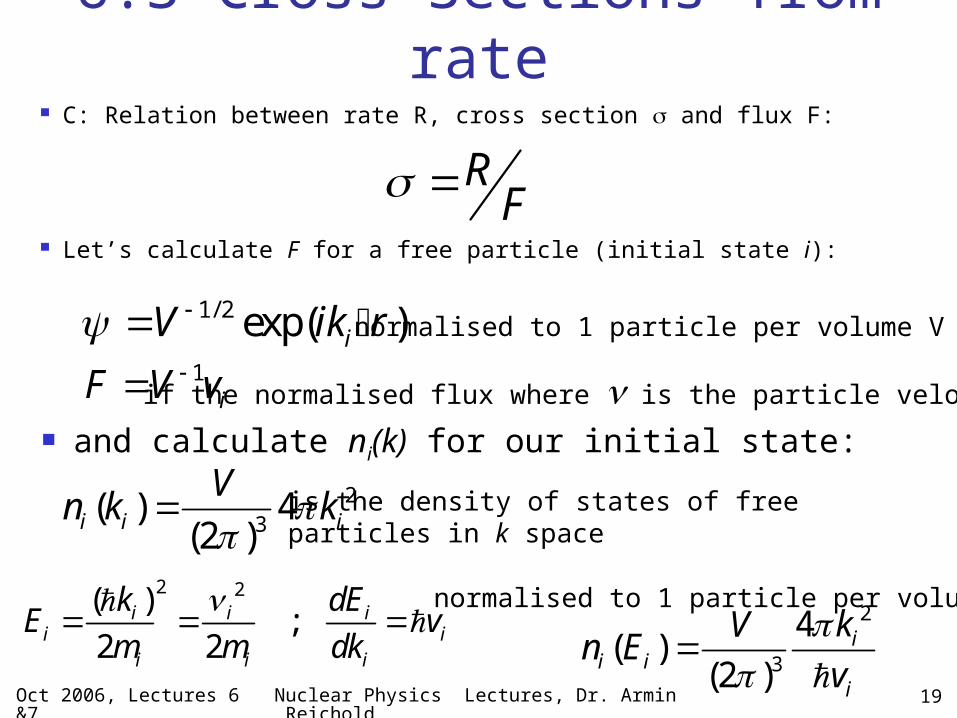
6.3 Cross Sections from rate C: Relation between rate R, cross section and flux F:

RF

23

( ) 4(2 )i i i

Vn k k

2 2( );

2 2i i i

i ii i i

k dEE v

m m dk

2

3

4( )

(2 )i

i ii

kVn E

v

Let’s calculate F for a free particle (initial state i):1/ 2 exp( )iV ik r

normalised to 1 particle per volume V

1iF V v if the normalised flux where is the particle velocity

is the density of states of free particles in k space

normalised to 1 particle per volume V

and calculate ni(k) for our initial state:

Oct 2006, Lectures 6&7 20

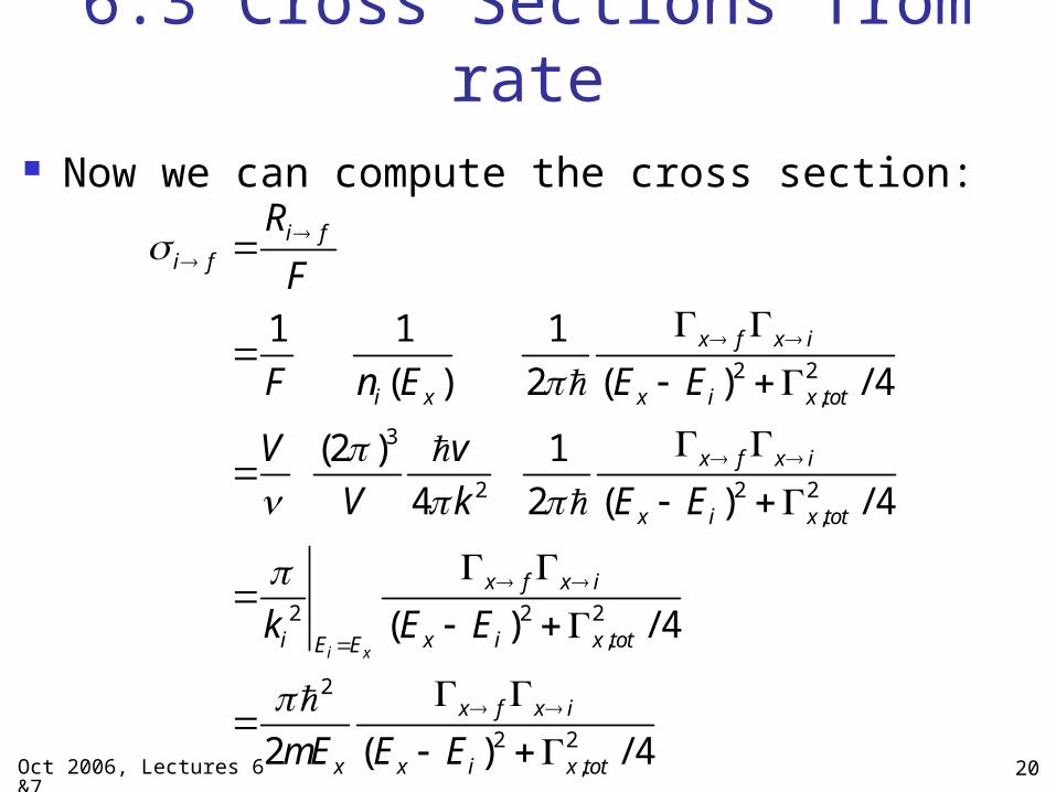
6.3 Cross Sections from rate Now we can compute the cross section:

2 2,

3

2 2 2,

2 2 2,

2

2 2,

1 1 1

( ) 2 ( ) / 4

(2 ) 1

4 2 ( ) / 4

( ) / 4

2 ( ) / 4

i x

i fi f

x f x i

i x x i x tot

x f x i

x i x tot

x f x i

i x i x totE E

x f x i

x x i x tot

R

F

F n E E E

V v

V k E E

k E E

mE E E


21

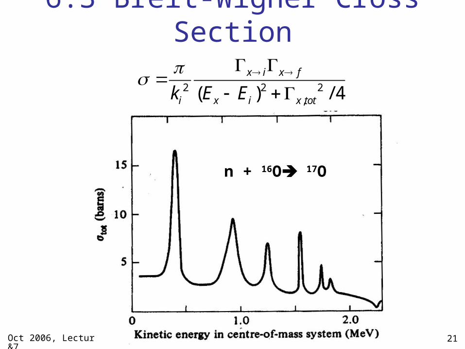
6.3 Breit-Wigner Cross Section

2 2 2,( ) / 4

x i x f

i x i x totk E E

n + 16O 17O


22

6.4 Rutherford Scattering i)

What do we want to describe: Scattering between two spin less nuclei due to Coulomb interactions Non relativistic scattering energies (Ecm<< smallest of the two

nuclear masses) Use the Born approximation

plane waves going into and coming out of scattering no disturbance of wave functions during the scattering acceleration happens at one instance in time nuclei stay what they were (no break-up or emission of other particles

etc.) First nucleus, denoted by i1 and f1

is light compared to the first one to guarantee no recoil has charge Z1

Second nucleus denoted by i2 and f2 is heavy no recoil is stationary in the lab frame before collision has charge Z2

Do this quantum mechanically and not classically. You would get the right result but by accident!

Good book for this is: “Basic Ideas and Concepts in Nuclear Physics”, K. Heyde, page 51-54

Oct 2006, Lectures 6&7 23result of d integration

6.4 Rutherford Scattering (computing Hfi)

The scattering potential in natural units:2

1 2

0

( ) ; ; 1 in what follows4

Z Z c eV r c

r c

1/ 2 1/ 21 1exp( . ) ; exp( . )i i f fV ik r V ik r

1 31 21 1

exp( . ) exp( . )fi i f

all space

Z ZH V ik r ik r d r

r

1 1i fq k k

1 31 2

exp( . )fi

all space

iq rH V Z Z d r

r

11 2

1 2

0 1

exp( cos )2 cosfi

iqrH V Z Z r dr d

r

The wavefunction of the incoming and outgoing first nucleus:

The matrix elements of the Coulomb interaction Hamiltonian:

chance variables:

Choosing z-axis parallel to q:


6.4 Rutherford Scattering (computing Hfi)

1 21 2

0

11 2

0

11 2

0

exp( )2

12 exp( )

12 [exp( ) exp( ) ]

iqr

fi

iqr

iqr

iqr

z dzH V Z Z r dr

r iqr

V Z Z z dz driq

V Z Z iqr iqr driq

exp( / ) lim( )r a a now multiply integrand by and take

1 1 2

0

2 1 1lim exp( ) exp( )fia

Z ZH V iq r iq rdra aiq

1 11 2 1 22

2 2 21 1lim

1 1fia

Z Z Z ZH V V

iq iqiq iqa a

Substitute: cos and cos dzz iqr d iqr


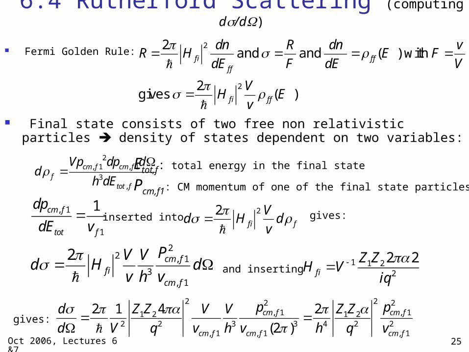
6.4 Rutherford Scattering (computing d/d)

Fermi Golden Rule:2

2

2( )

2( )

fi f ff f

fi f f

dn R dn vR H E F

dE F dE V

VH E

v

and and with

gives

2, 1 , 1

3,

cm f cm ff

tot f

Vp dp dd

h dE

2 22 2, 1 , 11 2 1 2

2 2 3 3 4 2 2, 1 , 1 , 1

42 1 2

(2 )cm f cm f

cm f cm f cm f

p pZ Z Z Zd V V

d V q v h v h q v

Final state consists of two free non relativistic particles density of states dependent on two variables:

Etot,f: total energy in the final state

Pcm,f1: CM momentum of one of the final state particles

22fi f

Vd H d

v

, 1

1

1cm f

tot f

dp

dE v inserted into gives:

22 , 1

3, 1

2 cm ffi

cm f

PV Vd H d

v h v

and inserting

1 1 22

2 2fi

Z ZH V

iq

gives:


26

6.4 Rutherford Scattering (computing d/d)

We now want to see the depedence on the scattering angle :

21 2

4 2 4 2, 1 , 1

( ) 1

8 sin ( / 2)cm f cm f

Z Zd

d h p v

2 2 2 2 2 21 1 , 1 , 1( ) 2 (1 cos ) 4 sin ( / 2)i f cm f cm fq p p p p

pi1pf1

2 2, 11 2

4 2 2, 1

2 cm f

cm f

pZ Zd

d h q v

inserted into:


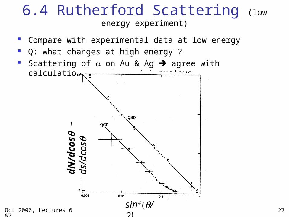
6.4 Rutherford Scattering (low energy experiment)

Compare with experimental data at low energy Q: what changes at high energy ? Scattering of on Au & Ag agree with calculation

assuming point nucleus

sin4(/2)

dN/dcos~

ds/

dcos


28

6.4 Rutherford Scattering (high energy experiment)

Deviation from Rutherford scattering at higher energy determine charge

distribution in the nucleus.

Similarity to diffraction pattern in optics

Form factor is F.T. of charge distribution

Electron – Gold scattering

a’la Rutherford

looks like a diffraction pattern on top of a falling line


29

6.4 Thinking about the last two lectures

What would happen to drutherford/d if: Vcoulomb-Vcoulomb Vcoulomb were ~ 1/r2

2 2

-151 22

0 0

2 -15

( ) ; ; 2.8 10 4 4

2.8 10 0.511

ee

e e

Z Z c e eV r E r m L

r c m c

c r m c m MeV

if tot=sum(partial), is the width of the energy distribution for decays into a single decay channel only a fraction of the total width

oct 2006, lectures 6&7 nuclear physics lectures, dr. armin reichold 1 lectures 6 & 7 cross...

Documents

n b dx

n b particles of type

n b slide

particles of type b

target b atom

nuclear physics lectures

reaction rates n

mass energy b