oct. 1 5 , 2017. on some sums of digamma and polygamma
TRANSCRIPT
Oct. 15, 2017.
1
On Some Sums of Digamma and Polygamma Functions – Revision (2017) and Review
Michael Milgram*,
Consulting Physicist, Geometrics Unlimited, Ltd.,
Box 1484, Deep River, Ont. Canada. K0J 1P0
Abstract: This paper is an enhanced version of a more than decade-older paper with a similar title. Many formulae involving both finite and infinite sums of digamma and polygamma functions up to quadratic order, few of which appear in standard reference works or the literature, but which periodically arise in applications, are collected, reviewed, listed and developed to the point that a knowledgeable reader could devise a formal proof. Several errors in the literature are corrected. Author’s Note (2017 version): The forerunner of this paper was originally consigned to arXiv in 2004 after being rejected by several reputable journals, mostly on the grounds that the contents were well-known, although one referee felt it necessary to opine that the author lacked a “prestigious affiliation”. Over the intervening years, the arXiv entry (https://arxiv.org/abs/math/0406338) has garnered a reasonable number of citations in the published literature, thereby demonstrating a need for an easily accessible reference work, and the author has attempted to improve the prestige of his affiliation. Also, since that time, a number of results, particularly for finite sums, have been obtained that may be either not-so-well-known or new, many of which are needed for applications (e.g. [31]). At the same time, new results for Euler (harmonic) sums have independently appeared in the literature, but the correspondence between two equivalent results, one expressed as a sum of (powers of) harmonic numbers, the other as a sum of (powers or products of) digamma or polygamma functions is not always transparent, recognizable or easily determined. Thus, I have prepared this enhanced version of the original 2004 paper, containing a large number of additional, possibly new, results, intended to be used as a reference or review. As before, the emphasis has been on generalized Euler-type sums – that is, sums where the summand contains at least one digamma or polygamma function, and one or more independent parameters, but contains a minimal number (or no) Gamma-functions, except as needed for derivations. With specialized applications in mind, the results are limited to quadratic forms, although a few cubic forms are included when needed for simplification. Transcriptions of all the new additions have been checked by copying each formula from the text by hand and verifying numerically using the Maple computer code. Note that the equation numbers in this and the original version do not always match, although the main text – Sections 1 to 3 – has only been modified slightly. In particular, Appendix B is now devoted to results for finite series. It is interesting to note that some results are closed, rather than consisting of transformations between series. A new Appendix C (mostly) repeats the previous listings of infinite series with some additions, again with only hints at the proofs. Appendix D consists of a computer-generated result that was too complicated to transcribe accurately and Appendix E lists a few simple specific and useful results extracted from the more general entries and the literature, regarding which, several corrections are noted. References to now-long-ago-published results, cited previously as unpublished, have also been updated. In general, within * [email protected]
Oct. 15, 2017.
2
sections, results are listed in order of increasing complexity with only the barest of hints at proofs, except for some cases which are grouped together so that (implied) proofs might become more transparent. Abstract(2004): Many formula involving sums of digamma and polygamma functions, few of which appear in standard reference works or the literature, but which periodically arise in applications, are collected and developed. Along the way, a new evaluation for some members of the family of hypergeometric functions – 4F3(1) – is presented, and a connection is made with Euler sums.
1. Introduction Although sums of digamma functions often appear in applications such as particle transport
[19] and the evaluation of Feynman diagrams [7,24,25] there is a paucity of results available in the standard references [12, 26] or in the literature [3,9,13, 24, 27] except for the special case of Euler or harmonic sums [e.g. 10]. Therefore, many formulae are often revisited by different authors [e.g. 27] because no repository of quotable results exists. At the same time, many such sums are very slow to converge, so it is important to obtain closed form expressions when numerical evaluation is intended. The purpose of this paper is to collect and develop, in one place, a number of sums involving digamma and polygamma functions that have arisen in applications [e.g. 19 and 31] or which were obtained as a byproduct of those endeavours. Although many of the results about to be quoted are easily established by evaluating parametric derivatives of hypergeometric functions of unit argument - a technique that “traces back to Newton” [6] - it is believed that many of them, which generalize previously known results, are also new. To keep the paper to a reasonable length, proofs are only sketched, sufficiently that a knowledgeable reader, with access to a computer algebra program, should be able to reproduce them. By way of review, the digamma function )( x is defined by
))(log()( xdxdx
(1)
so that
)()()( xxxdxd
(2)
with*
1
1( ) ( ), 0.( )
k
lx x k k
x l
(3)
Polygamma functions are written as:
( )( ) ( ) and ( ) ( ) if 2n
nn
d dx x x x ndx dx
(4)
* see also (7).

Oct. 15, 2017.
3
Two useful, well-established results, used throughout, are
)/())()1()()1(()(
1)(
10
abbbkaakba
k
(5)
and
abifa
abbababa
)(
)/())()(()(
1)(
10
(6)
Also, define generalized harmonic numbers [27, 6, 35]
1
1( ) ( ) ( )( 1)
n
nl
H a n a al a
(7)
together with
21
1( ) ( ( ) ( ) ).( 1)
n
nl
H a n a al a
(8)
In general, if 0k , commonly used variants are 1
( ) ( 1) ( 1)
1
1 ( 1)(1) ( 1) (1)( )
( ),kn
k k kn k
lH n
l k
(9)
1
( ) ( 1) ( 1)1 1 12 2 21
1 2
1 ( 1)( ) ( ) ( )( ) ( )
( )kn
k k kn k
lH n
l k
(10)
and, with respect to the corresponding alternating series, ( ) ( 1) (1 ) ( 1) (1 ) ( 1)1
21
(1 )1,
( 1) ( 1)(1) ( 1) [ ( 1) 2 ( 1)] (2 1) (1)( )
2 (1 ( 1) ) ln(2)
(
) .
l knk n k k k k k
n kl
k nk
L n nl k
(11)
Throughout, )(n is Riemann’s zeta function, 1,k is the Kronecker delta, ),( cs is the Hurwitz
zeta function, )1( is the Euler-Mascheroni constant and 1
( )l
n nl
xLi xl
is the nth polylog
function. Symbols starting with the letters “j” through “n” are always non-negative integers. All
other symbols are continuous and (arbitrarily) complex.
0 0l l
and
2
1
0n
nl
if 2 1n n
(except see (B.22)). G is Catalan’s constant and x symbolizes the “floor” function (greatest integer less than or equal to x).

Oct. 15, 2017.
4
2. Hypergeometric Sums Lemma 2.1. An easily obtained and useful sum needed later (see (63)), which generalizes a well-known result [18, Eq. 3.13(43), 26, Eqs. 7.4.4.40-46], which is not listed in any of the standard tables, [26, 34] and which is a special case of a more general result [26, Eq. 7.4.4.11 or 7.4.4.3] follows:
.1
0 )1)(()(
)1())()1()(1(
)()()1(
)
()|( 1,2,1,1
23
n
l lnlnlnnnn
nnF
(12)
Proof: Write the 3F2 as a convergent sum with )()( , change the lower summation limit from “0” to “-n”, subtracting equal terms, to get:
.)(1
00
023
)1)(()(
)1)(()(
)()()1(
)1)(()(
)()()1(1
,2,1,1 )|(
n
ll
l
lnlnl
lnlnln
nllln
nnF
(13)
The first infinite sum in the second equality is recognized as a 3F2 with known summation [18, Eq. 3.13(43)]. (12) follows immediately, for all values of and by the principle of analytic continuation. § Lemma 2.2 Another useful result needed later (see (63)) that does not appear in the standard tables, (however, see [22]) but which is a special case of a known result [26, Eq. 7.4.4.11] is
.)1()(
)1()()1()1()(
1,1,
,,
1
23
0 )2()()()1)((
)|(
n
nbcnanban
nbcnbc
accbacb
cbncba
n
nF
(14)
Proof: With )()1( n , apply the well-known result [18, Eq. 3.13(38)] n-times repeatedly and use Gauss’ formula for a 2F1 of unit argument. § Corollary: Evaluate the limit a=1 in (9:

Oct. 15, 2017.
5
2
0,
)2()()1()1)(1(
)1()(
)()()()())()((1
,1,,,1 )|(23
n
nbcnnbn
nbcnbc
ncbbcbbncbc
cbncbF
(15)
reducing to [26, Eq. 7.4.4(33)] when n=1. Theorem 2.1 The following terminating sum only appears symbolically in the literature as a limiting case of a very complicated result [26, Eq. 7.10.2(9)], or for special values of “c” (e.g. [29, Eq. (3.4)]):
.)(
)(
0
034
)()1()()1()2(
)1(
)1()2()()1(
)1()1(
)1|(
)(
)(1,2,2,1,1,1
k
l
k
l
lclckck
kc
kcllc
kcF
ck
(16a) (16b)
The two forms of (16) are obtained from one another using (21) below. The derivation depends on results to be obtained in Section 4, but this result is listed here for consistency of presentation. The proof is outlined in Appendix A. Theorem 2.2 Similarly, the following, which only appears in the tables as an exceptional, limiting case of a very complicated result [26, Eq. 7.10.2(2)], is easily obtained by rewriting (C.20).
.0)
1,2,21,1,1,1
1(,)1)(2()1(
)2()1()(
)3(2)](][(6
)([)()1|(1
0
2)2(
21
34
qlllq
lq
qqqFq
l
l
q
(17)
If 1, nnq , the infinite series terminates at 2l n . Theorem 2.3 Likewise, the following results do not appear in the literature.

Oct. 15, 2017.
6
1
0 21
212
21
21
21
2
21)2(
21
27
3421
)(1
)(1)1(
)()1(
)()(2
)()3()1|()(
12/3,2,2
1,1,1,1
n
l nlll
nll
nnnFn n
(18)
1
0 21
212
21
21
21
23
212
21)2(
21
3421
)(1
)(1)1(
)()1(
)(2log22)(
2log)()()3()1|()(
127
2/3,2,21,1,1,1
n
l nlll
ll
nn
nnFn n
(19)
)2log1(2
)3()1|(2
34 47
2/1,2,21,1,1,1
F
2log2
)3()1|(2
34 47
2/3,2,21,1,1,1
F
(20a)
(20b)
Proof: Set nq 2
1 in (C.20) employing (3) and (C.23). § In (19), since the series representation of the left-hand side does not converge for 2n , the right-hand side represents the left-hand side* in the sense of analytic continuation, because the variable “q” is continuous in (C.20) (whose left-hand side is a valid representation of the hypergeometric function for this range of the variable “n”). (20a) is a simple restatement and simplification of (19) using n=1. The case n=0, (20b), corresponds to the special case 0 baof [15, Eq.7].
3. Finite sums involving Digamma functions Theorem 3.1
An important duality exists between two finite sums of digamma functions (see also (B.6)):
.)1()()()1()1()(00
k
l
k
l lblccbkbkc
lclb
(21)
Proof: Expand, rearrange, and with reference to (3) and (5), find:
* i.e. )1|(
2/3,2,21,1,1,1
34 nF
means 0,)1|(
2/3,2,21,1,1,1lim
34
nFqnq
.
Oct. 15, 2017.
7
kckb
cb
cb
cb
lclbk
l
)(2
)2(1
)1()()(0
)/())(()1/())((
)/())((
21
111
11
21
111
cbkcbkcb
kbbb
kbkbbb
(22)
,)1()1())()1()((1
0
k
l lblckcckcb
from which (21) follows immediately. §
Using (3), the sums on either side of the equality can be reduced to one another when “b” and “c” are separated by integers, showing that a closed sum exists for those cases (cf. (26) and (B.3)). Another, equivalent form of (21) can be easily found by rearrangement:
.)()()1()1(
)()()1()1())()((0
cbcb
cbkckb
cbkbkclblc
lclbk
l
(23)
A useful [19] special case is given below:
k
l
k
l llkk
ll
1 212
121
0
21 )1()()1()2()(
1)(
(24)
Corollary
Apply (3) to (21) and simplify to obtain an equivalent form in terms of generalized harmonic numbers [6, 35]:
)1()()1(1)(1
112
1
0 21
021
kk
k
ll
k
ll HHH
lH
l (25)
Also see [30, Theorem 7, Example 2]. Theorem 3.2 (See also (B.9))
])()1()()1([)()( 22
21
0bkbbkb
lblbk
l
(26)
Proof: Start from [12, Eq.7.1.1]
Oct. 15, 2017.
8
)1/())1(
)()(
)1(()())(
0
aba
bka
kblalbk
l (27)
and operate on both sides with b giving an interim result worth noting:
.)1/())1(
)()(
)1((
)1/())1()()(
)()1()1((
)()()(
2
0
aba
bka
kb
aba
bbka
kbkbla
lblbk
l
(28)
Then evaluate the limit ab+1 to get (26). Alternatively, take the limit c=b in (23). § In applications, the cases b=1 and b=1/2, both of which are easily obtained from (26), arise.* Notably, the case b=1 extends an unfinished sum† and integral from the standard tables [12, Eqs. (55.2.1) and (5.13.17)] as follows:
21
0
1
02
221
11
1
0
)1(1
)1(1
21
)]1()1())1()1([(11)1log(1
1
k
l
k
l
l
m
k
l
k
ll
kkml
dtttt
(29)
specializing‡ a recently quoted general result for non-integral values of “k” [3, Eqs.(3.6) and (3.9)]:
)]1()1())1()1([(
)()()1log(11
221
2 1
11
0
xx
mmxdtt
tt
l ml
lx
(30)
4. Infinite Series
For completeness, a well-known sum, recently revisited [27, Eq. (2.7)], is quoted. If
0)( bc ,
})]()([)({)()())1()((
)()(
1 bbccbc
cb
lblb
lclb
l
(31)
* Curiously, the computer code Maple 6 (and Maple 2016) found the b=1 version of (the new result) (26), but missed all other possibilities tested. Mathematica [34,Version 4.1 (~2004)] missed all possibilities tested, but Mathematica [10, version(2016)] correctly found this result. † reproducing a known result [1, Lemma 1] in this special case. ‡ Note the relationship between the inner sum in (30) and (67).

Oct. 15, 2017.
9
Set c=b+1, and change the notation slightly, giving
)]}1()1()[(6
{1)1()1(
)1( 2
0
bbblbl
lbl
. (32)
In the limit b0 this reduces to a very well-known result [9,24, 34]
6)3(
)1()1( 2
02
l ll (33)
Theorem 4.1 Consider a useful variant of (32):
})()()()({)(2
1))((
)1( 22
0
qqpppqqlpl
ll
(34)
Proof: Temporarily, assume 1)( , and consider
))1(
)()1(
)()(
)1()(
)1()1()()()1(
)1()()(
)(1
])(
1)(
1[)1()(
)(1
))((1
)1()(
(
][1
,1
,1212
00
pp
pq
Fq
qFp
ppq
qlplll
pqqlplll
pp
ll
(35)
using Gauss’ summation for a 2F1 of unit argument. The condition on may now be relaxed. Operate on both sides of (35) with
1lim , respectively reducing the left- and right-hand sides
to the corresponding sides of (34). § The sums (enclosed in square brackets) in these results diverge if they are considered individually when 1)( , so that a careful adherence to the ordering of limits, and the use of the principle of analytic continuation is needed. Corollary The following generalizes (33)
)()()()()1( )2(
21
02 qqq
qll
l
(36)
Proof: Evaluate the limit qp in (34). § See also (66) and ( .

Oct. 15, 2017.
10
Corollary
1
0
22
22
0
)1)(1()1()()()()()()(
2/))()()()(()(
1))(()1(
}
{m
l
l
lqlplmqqmppqp
qqpppqqlpl
ml
(37)
Proof: Using (3) and (6) assume mqp ,2,1, and split the following sum using partial fractions
1
0
1
0
1
0
1
0 0
))(()(1
)()(1
)()(
))()((1
m
l
m
l
m
l
m
k l
lmplmqlm
lmqpqq
lmppqp
kmlqlpl
(38)
The first two sums are easily evaluated; reverse the third right-side sum, apply (34) to the finite sum on the left and eventually arrive at (37). § The conditions on p and q can be relaxed by taking the appropriate limits. A limit must also be evaluated when p and q are separated by integers. In particular, many results, laboriously and individually derived elsewhere [24] are special cases of (37). Also, if p and q are integers, the finite sum in (37) can be evaluated in closed form using (26) – also see (B.3), (B.16), (C.6)) and (C.7) as well as Xu [36]). Theorem 4.2
))1()1()(1(
)1()1()1()1(21),(
where),(1
)]()([
)( 22
0
q
qqq
ql
llql
(39)
Proof: Consider the following sum with )()( :
3 2 3 20
,1,1 ,1,1, 2 , 2
( ) ( ) 1 ( ) ( )( |1) ( |1)( ) ( ) ( 1) ( ) ( )
( 1) ( 1) ( 1) ( 1)( 1) ( 1) ( )( 1) ( 1) ( 1) ( 1)
[ ]
( )l
q l l q bF Fq l l l q a
x qq bx q
(40)

Oct. 15, 2017.
11
using a well-known result [18, Eq. 3.13(43)] to sum the hypergeometric functions. Relax the constraint and operate on both sides of (40 with
lim so that the right- and left-hand sides
become the corresponding sides of (39). § As before, the two terms in (40) correspond to divergent series if written individually; this is indicated by the use of square brackets as a reminder, and again new results can be obtained by
operating with and/or
q
and taking appropriate limits. For example, the limit 1 in
(39) yields
2/)()())1()(()1(
)1()1( )( 212
0
qql
llql
(41)
and operating with q
on (41) with some reordering gives
.)1()1()1()1()1(21
)1()( )2(
0
qqqql
lql
(42)
Take the limit q=1 to recover the special case
)3(2)1()1(
0
l ll
, (43)
corresponding to a known result [24], [12, Eq. 55.9.7). Theorem 4.3 Eq. (39) can be generalized further.
1
00 1)()(),(
1)]()([ m
ll lmlmlqqm
mlllq
(44)
Proof: Add and subtract terms corresponding to 1,, ml in (39) and re-order the resulting series. § Corollary: (44) reduces to the following useful result by setting 2
1m and 21q .

Oct. 15, 2017.
12
1
0
21
21
21
2221
21
0
21
)1()(
)1()()()1(2
)1()1()()1()1(
)]()1([
)(
)(
m
l
l
ll
mmml
mlml
(45)
See also (24). Theorem 4.4 For completeness’ sake, a known variation of (31) [27, Eq. (2.14)] is quoted, without proof.
)( )1()1()1()()1()1()()1(
)()(
0
pqpqpp
qpqllplq
l
(46)
Using methods similar to those already employed (e.g. Theorem 4.2), other variants of (31) and (46) can be obtained:
]
[
)]()1()[1(
)1()()1()1(
)1)(()()(
0
qppp
pqppq
llplplq
l
(47)
and
]
[
)1()()]()1([2
)]()1([)1(2
)1()1)(()1()( 2
0
pqpqpp
qppp
qllpllq
l
(48)
Theorem 4.5
0
0
}
{
)1)(1()1()2()1)((
)()()()2(
)()()1()1()(
)1(
))1((
)1()()(
)()( )1(
1
l
l
l
lclpllclcf
cffpcpf
fpcfcff
p
f
cpclf
lplc cp
(49)
Proof: Consider the sum
)1|()()()()(
)()()()(
,,,1
230 fp
cFfp
clflpllc
l
(50)
Convert the hypergeometric 3F2 into another 3F2 having the property that it terminates if mp , (m>1) according to [18, section 3.13.3]
Oct. 15, 2017.
13
}
{
)1|(
)()()()1()(
)()1()()1()1|(
2,11,2,
,,,1
23
23
)1()1()1()1(
ccfcpcf
fpc
F
fcpcfcf
ppcfpF
pcfcf
(51)
Operate on both sides with
flim
and simplify. §
This derivation of (49) is valid for all continuous values of p , although it is not particularly useful unless the infinite series (equivalent to a 3F2) can be summed analytically (e.g. mp , an integer, in which case the infinite series terminates). If f=1, it can be shown, by summing the infinite series [26, Eq.7.4.4.(49)] and taking the appropriate limit, that (49) reduces to (46) as a special case.
To obtain other useful results from (49), operate with ff
1lim
. Then set 2p giving
,)1()1()1()1()2(
)1()( )( 2212
412
21
21
0
qqqql
lqll
(52)
reducing to (43) when q=1. Alternatively, operate on (49) with
ffcp
1lim
1lim , and from the requirement that the coefficient
of 1)1( cp on the right-hand side must vanish (series converges), find
0
2
2 6cot)(
sin)(
))(1()()(
lqq
lqlqlql
, (53)
reducing to (33) when 1q . See also (C.19) to (C.23). Lemma 4.6 The following sums the difference of two divergent series (see also (C.43) and (C.44)).
3)1()( 2
0 21
21
l l
ll (54)
Proof: Consider the following sum (with 0)( ):
Oct. 15, 2017.
14
.)1|()(
)()()1|(
)()()1()(
)()()1()(
2/32/1,
2/32/1,1
1223
21
1223
21
0 23
21
21
FF
llllll
l
(55)
As before, sum the hypergeometric series, relax the limitation on and, with deference to the
principle of analytic continuation, operate on both sides with
1lim
. §
Theorem 4.7 The following generalizes (54) (also see (C.9) etc.):
12 1 1 1
2 2 210 2
2 121 1
2 2 11 2
( ) ( 1) ( ) ( ) ( ( ) 4)( ( ) ( ))
( )( ) 8 4 ( ) 26 ( )
[ ]l
k
l
l k l k k k k kl
ll
(56)
Proof: Let
0 21
21 )1()(
lk l
klklV
(57)
Then
1)()()()(
)1)(11( 21
21
21
21
121
0 211
kk
kk
Vlklkl
VV kl
kk
(58)
Apply (58) repeatedly (k times), giving
31)()()()( 2
01
21
21
21
21
0 )(
Vwithl
ll
lVV
k
lk (59)
The second term enclosed by brackets in (59) equals .12/2 lif Use (54) and its analogues, and, after some simplification, including the use of (21), find (56). § See also (45). Theorem 4.8
2/)()()()()()(
)()( }){}({ 22
0
][ aaqaqaqlaqla
lala
l
(60)
Proof: Since this is effectively the (finite) difference between diverging sums, consider the following two converging sums, subject to the condition )()( a :
Oct. 15, 2017.
15
)1|()1(
)()1|()1(
)()1(
)())1(
)(
11,
11,
1212
00][
qaq
aF
qaqF
a
qlaql
lal
ll
(61)
As in previous cases, evaluate the two hypergeometric functions independently, simplify, and
operate with
. Then, unite the two sums into one (convergent) sum, and evaluate the limit
a . § Notice that, to within a constant, each of the terms of (60) that are enclosed in braces ({ }) regularize corresponding divergent series on the left. Also, see (C.8) and (C.14). Corollary
)()()()(
)()()( )2(
21
02 qqq
lqlq
lqlq
l
(62)
Proof: Operate with qa
0lim
on (60); alternatively, operate withbkqb
limlim on (26). §
Theorem 4.9
n
l
l
nlcl
nccncnc
nccn
lcln
lnlc
0
2
2
0
)1()1(2
)1()()1()1(
)1(1)()1(
3)()1(
)1()( )(][
(63)
Proof: Consider the following sum with 0)( c . With this restriction, the sum may be split into two and identified:
)1|()1()(
)1()1|()()1(
)())(1()1(
)1)(()(
1,11,,1
2,,1,1
2323
0][
cncnc
ncn F
nccnF
cn
lclncnl
lnlcl
l
(64)
Using (12) and (9, each of the hypergeometric functions can be summed, and the restriction relaxed by the principle of analytic continuation. Since the combined sums converge, operate on
both sides with
clim
and sum a terminating 3F2, giving

Oct. 15, 2017.
16
)1|()()1(
)()1(
)()(),1(
)()()1()1(3)(
)1()1(
)(
2,2,11,1,1,1
34
1
0
2
2
0
)(][
ncnF
ncn
lnlc
ncncncnc
nccnnclcln
lnlc
n
l
l
(65)
From either version of (16), the 4F3 can be identified, and Eq. (63) emerges after considerable simplification. § See also (B.16). In the limit 1 nc , both sides of (63) and (65) vanish. This has been verified and a known, closed-form for a special case of the resulting 4F3 has been retrieved. Theorem 4.10 (generalized Euler sums [10] and polylogarithms [16]. See also (C.14).
2,)()()()!1(
)1()()1( )(
21
2
0
)2()1(
0
2
nqqqnql
l nn
k
knkn
ln k
n (66)
Proof: Operate on (36) with 2
2
n
n
dq. §
Using ( ) 1(1) ( 1) ! ( 1)n n n n and setting q=1 gives a simple derivation for an equivalent
form of Euler’s (linear) sum:
2
10
)()1()1(1)1()
21(
)1()1()2( n
kln knkknnn
ll
(67)
which, when compared to the form usually quoted in the literature [1, Eq. 20], [10, Theorem 2.2], yields the interesting relation
2 2
1 1
2( 1) ( ) ( 1) ( ),( 1)n n
k kk n k k k n kn
(67a)
a result that is true for any indexed function (proof by reversing the right-hand sum). Xu [36, Eqs. (1.27) and (1.28) – incorrect – add a term 11/ sa to the latter) has recently obtained an equivalent form of (66) as have Sofo and Cvijovo ́ [28, Theorem 1]. Special cases of (66) with combinations of 1
20 , , 1 a n d 2 , 3q n can be found in Appendix E; for example, set n=3 in (66) to retrieve the well-known harmonic result [9, Eq. (17)]:
4
30
( 1) (1) .( 1) 360l
ll
(68)
Finally, by taking the limit q m in (66) using 2n we find
2 (2)2
1
1 .3 2(1 ) ( 1)( ( 1)) ( 1)
( )ll m
ml m m m
l m
(69)
Oct. 15, 2017.
17
Split the sum into its finite and infinite parts, apply the limit 0q to (C.6) and compare the resulting infinite sums to obtain (B.68).
Variations of Euler (quadratic) sums are available by operating on (47) withqq
1
lim
:
2
0
( ) ( 1) 1 [ ( ) ( 1)] ( ) ( 1)[ ( ) ]( )(1 ) ( 1) 6
2 (3) ( 1) ( )
(
)l
q l q l q q q q qq l l q
q q
(70)
reducing – after considerable simplification - to a known result [9, Eq.(9)], [16, Eq.(8.92)] when
1q :
36011
)1()]1()1([ 4
02
2
l ll (71)
Notice that the left-hand side of (70) can be rewritten as a transformation by a simple single step recursion, that is
2
20 0 0
( ) ( 1) ( ) ( ) ,( )(1 ) ( )(1 ) ( ) (1 )l l l
q l q l q l q lq l l q l l q l l
(70a)
and so, in the limit 1q
2 2 2 4
2 30 0
(1 ) (1 ) 3 (3)(1 ) (1 ) 6 30l l
l ll l
(72)
equivalent to Euler sums of weight (2,2) and (1,3), both of which are known (e.g. [5], [9]). Alternatively, simple differentiation of (47) with respect to the variable q with (p>q+1) produces
0
(2)
( ) ( ) ( ) ( 1) [ ( 1) ( ) ( 1)( )(1 ) ( 1)
( 1)( ( 1) ( ))}( 1) ( ) ( )] ,
{l
q l p l q l q q p q pp l l p
p p p qp p q p q
(73)
reducing to (70) when p=q+1. Similarly, operating on (48) with qpqp
1
lim gives
2 24 2
0
4 2(2)
2 23 (2) 2
( ) ( 1) (1 ) 1 5 3( ) ( ) ( ( ) )( )(1 ) 2 12 2 2
1 11( )( ( ) 4 (3)) ( ) / ( 1)2 180 6
1 3 1( ) ( )( ( ) ) ( ) (3) / ( 1)2 2 4 2 2
(
)
( )
l
q l q l l q q qq l l
q q q q
q q q q q
(74)
In the limit q=1, a straightforward result is

Oct. 15, 2017.
18
0
2
2
)1()1()2(
l lll (75)
Using this technique, along with (3), variations in the choice of nqp
lim and partial fraction
decomposition, all Euler sums up to cubic order become accessible. The use of computer algebra is recommended. Theorem 4.11
]
[
)](2)[1()1()1()]()1(2)[1(
6)1)(1()()1|(
)()(
)()1()(
2
22
340
2
,2,2,1,1,1
cpcpcpcpcp
cppcF
pc
lpllc
pcp
l
(76)
and
4 30
1,1,1,2, 2,
( ) (1 ) ( ) ( )( |1) ( 1)( ) ( ) ( 1)( 1 )
[ ( 1) ( 1 )][ ( 1) ( )]
(
)l
p cp
c l l c cF pp l p p p c
p p c p c
(77)
Proof: Following the method of Theorem 4.5, operate on both sides of (50) and (51) with both
2
2lim1
lim
ffand 2
2lim1
lim
ff
. The resulting expressions contain a large number of
terms, all of which can be evaluated (with computer algebra) using results given elsewhere in this paper, especially (47) and (48). Add and subtract the resulting expressions. § For the case
1 cp , see (C.20). Note: – the version 2014 statement of (77) contained a transcription error. Seen from another viewpoint, subtracting (76) from (77) gives an alternative identification for a particular 4 3F (1) specifically
24 3
0
2 2
1,1,1,2, 2,
( ) ( )( |1) ( (1 ) (1 ) )2 ( ) ( )
( 1) ( 2( ( )) / 6 ), 1 and 1,2( 1)
l
cp
p p c lF l lp c p l
p p c p c cc
(78)
where ( 1) ( 1)c p after the substitution c p c , the significance of which will be discussed elsewhere (to be published). See also (16) and (B.43).
16 3 2 4 ( ) 3 2 7
72 4 13 ( ) 3 2 6 ( ) 5
Oct. 15, 2017.
19
Acknowledgements Although I had been thinking about updating this paper for some time, I am grateful to Prof. Lu Wei for motivating me to finally do so. I am also grateful to those (cited) authors who chose to make copies of their work freely and publicly accessible, and acknowledge the Researchgate computer algorithm which brought many of those papers to my attention. Some authors have chosen not to post freely available preprints or legally permitted offprints on public websites; citations to any such papers published after 2005 and only available behind a paywall, have been withheld. Please contact this author for further information.
References 1. Adamchik V., “On Stirling numbers and Euler Sums”, J. Comp. Appl. Math.,79,119-130 (1997). 2. Adegoke, K and Layeni, O., “New Finite and Infinite Summation Identities Involving the Generalized Harmonic Numbers”, https://arxiv.org/abs/1508.07345 (2015). 3. Borwein, J.M, Zucker, I.J and Boersma, J., “The evaluation of character Euler double sums”
(2004). available from: http://eprints.cecm.sfu.ca/archive/00000255/ 4. Choi, J., “Finite Summation Formulas Involving Binomial Coefficients, Harmonic Numbers
and Generalized Harmonic Numbers”, Journal of Inequalities and Applications, 2013:49 (2013).
5. Choi, J., “Summation Formulas Involving Binomial Coefficients, Harmonic Numbers and
Generalized Harmonic Numbers”, Abstract and Applied Analysis, Article Id 501906 (2014). http://dx.doi.org/10.1155/2014/501906.
6. Chu, W. and De Donno, L., “Hypergeometric Series and Harmonic Number Identities”,
http://www.arXiv.org: math CO/0403353, (2004). 7. Coffey, M.W., “On one-dimensional digamma and polygamma series related to the evaluation
of Feynman diagrams”, J. Computational and Applied Mathematics, 183 (2005) 84-100. doi:10.1016/j.cam.2005.01.003. Also available from https://arxiv.org/abs/math-ph/0505051.
8. Cvijovic, D., “Closed-form summations of certain hypergeometric-type series containing the
digamma function”, J.Phys. A: Math. Theor. 41, 1-7, (2008). Doi:10.1088/1751-8113/41/45/455205. Also available from https://www.researchgate.net/publication/231110852.
9. de Doelder, P.J., “On some series containing )()( yx and 2))()(( yx for certain
values of x and y”, J. Comp and Appl. Math., 37, 125-141 (1991). 10. Flajolet, P. and Salvy, B., “Euler Sums and Contour Integral Representations”, Experimental
Mathematics 7,1,15-35 (1997).

Oct. 15, 2017.
20
11. Glasser, Larry, (private communication), (2017). 12. Hansen, E.R, “A Table of Series and Products”, Prentice-Hall (1975). 13. Jordan, P.F., “Infinite Sums of Psi Functions”, Bull. American Math. Soc., 79,4,681-683
(1973). 14. Kölbig, K.S., “The polygamma function ψ(k)(x) for x=¼ and x=¾”, J. of Comp. and Appl.
Math., 75 (1996) 43-46. Doi:10.1016/S0377-0427(96)00055-6 15. Lavoie, J.L., “Some Summation Formulas for the Series 3F2(1)”, Math. Comp., 49,179,269-
274 (1987). 16. Lewin, L., “Polylogarithms and Associated Functions”, North Holland, (1981). 17. Liu H., Zhou, W. and Ding, S. “Generalized harmonic number summation formulae via
hypergeometric series and digamma functions”, Journal of Difference Equations and Applications”, 1-15, (2017). dx.doi.org/10.1080/10236198.2017.1318861 citation withheld (see acknowledgements)
18. Luke, Y., “The Special Functions and their Approximations, Vol. 1”, Academic Press (1969). 19. Milgram, M.S., “Identification and Properties of the Fundamental Expansion Functions for
Neutron Transport in an Infinite Homogeneous Scattering Medium”, Annals of Nuclear Energy, 32,11, 1167-1190, (2005). https://doi.org/10.1016/j.anucene.2005.02.015. Also available from https://www.researchgate.net/publication/239358548.
20. Milgram, M.S., “A Series Expansion for Integral Powers of Arctangent”, Integral
Transforms and Special Functions, 17, 7, 531-538 (2006); also available from http://www.arXiv.org: math:CA/0406337, (2004).
21. Milgram, M.S., “Powers of a Hypergeometric Function”, Integral Transforms and Special
Functions, 17,11, 829-832 (2006); also available from https://arxiv.org/abs/math/0505202 22. Milgram, M., “Comment on a paper of Rao et al., an entry of Ramanujan and a new 3F2(1)”,
J. of Computational and Applied Mathematics,201,1-2 (2007). https://doi.org/10.1016/j.cam.2006.01.025. Also available from
https://www.researchgate.net/publication/242980686 23. Milgram, M.S., “447 Instances of Hypergeometric 3F2(1)”, available from
https://arxiv.org/abs/1105.3126 (2011) and/or https://www.researchgate.net/publication/51891949_447.
24. Ogreid, O.M. and Osland, P.O., “More Series related to the Euler Series”, J. Comp. & Appl.
Math.,136, 389-403 (2001).
Oct. 15, 2017.
21
25. Ogreid, O.M. and Osland, P.O.,”Some Infinite Series Related to Feynman Diagrams”, J. Comp. & Appl. Math, 140, 659-671 (2002).
26. Prudnikov, A.P., Brychkov, Yu.A., Marichev, O.I., “Integrals and Series”, Vol.3, “More
Special Functions”, Gordon and Breach, 1990. 27. Rassias, T.M and Srivastava, H.M., “Some Classes of Infinite Series associated with the
Riemann Zeta and Polygamma functions and Generalized Harmonic Numbers”, Appl. Math. & Computation, 131, 593-605 (2002).
28. Sofo, A. and Cvijovi ́, “Extensions of Euler Harmonic Sums”, Appl. Anal. Discrete Math., 6 (317-328 (212). Available online at http://pefmath.etf.rs 29. Srivastava, H. M., Studies in Appl. Math., 86, pp. 79-86 (1992). 30 . Speiss, J., ”Some Identities Involving Harmonic Numbers”, Mathematics of Computation, 55, 192, 839-863 (1990). 31. Wei, Lu, “A Proof of Vivo-Pato-Oshanin’s Conjecture on the Fluctuation of von Neumann
Entropy”, Phys. Rev. E, 96, 022106 (2017). Also available from arXiv.org/abs/1706.08199 (June 26, 2017).
32. Wei,C., Yan,Q. and Gong,D., “A family of summation formulae involving harmonic
numbers”, Integral Transforms Spec. Funct. 26(2015) 667-677. http://dx.doi.org/10.1080/10652469.2015.1034124 citation withheld (see acknowledgements)
33. Wei, C., “Watson-type 3F2-Series and Summation Formulae Involving Generalized Harmonic
Numbers”, arXiv.org/abs/1607.01006 (July 3, 2016). 34. Wolfram, (2004): http://www.functions.wolfram.com/ 35. Wu, T.C., Tu, S-T, Srivastava, H.M., “Some Combinatorial Series Identities Associated with
the Digamma Function and Harmonic Numbers”, Appl. Math. Lett., 101-106 (2000). 36. Xu Ce, “Parametric Harmonic Number Identities”, arXiv.org/abs/1701.03726 (2017). 37. Xu C.,Yang, Y. and Zhang, J.,”Explicit Evaluation of quadratic Euler Sums”, International
Journal of Number Theory,(2017) doi: 10.1142/S1793042117500336. Also available from https://arxiv.org/abs/1609.04923. 38. Zheng,D.,”Further summation formulae related to generalized harmonic numbers”, J.Math.
Anal. Appl., 335 692-706, (2007). doi:10.1016/j.jmaa.2007.02.002.
Oct. 15, 2017.
22
Appendix A: Sketch of Proof of (16)* Proof: In (65), with 0)( c , set n=0, giving
2
2
0
( ) ( 1) ( )[ ] ( 1) ( ) ( )( 1) ( ) 3 ( 1)l
c l l cc c cl c l c
(A.1)
Split the infinite sum into two parts: ,0 kl , and 1kl , and shift the lower value of the summation index of the second (infinite) series to zero. The resulting infinite series, given by (65) with the replacement 1 kcc and 1 kn , involves a 4F3, so using (A.1) and (21), solve for the 4F3 and simplify. §
Appendix B: Finite Sums
The following useful and related finite sums, based on the methods of this paper, many of which are needed [e.g. 31]) or obtained elsewhere [19], are presented with minimal proof. From [21, Eq.(3)]
)1(2)()()(
2)(
)(21
21
1 1
21
21
21
kk
k
l
k
l
HHl
llk
l
(B.1)
From (B.5) (below), after some rearrangement and utilizing (26) obtain
122 1 1 1
1 12 2 210 02
3 11 12 2
( )( 1) ( ) ( )( ) 1
(1) ( ) 2 ( 2) ( )
k k
k kl l
k k
ll H Hk l l
H k H
(B.2)
and
6)2()2()2(
)1()1( 2
2
0
kkklk
lk
l (B.3)
which, after reversal, or with reference to (21), can also be written
22
1
( 1) ( 1) ( 1) ( 1) .6
k
l
k l k k kl
Also, see the case n in (B.53) below. Equivalently,
* A proof of (16) based on [26, Eq. 7.4.4(38)] might be attainable. However, that result fails several numerical tests, and appears to be incorrect.

Oct. 15, 2017.
23
1 1
0 0 0 02 2
21 1 1 12 2 1 22 2 2 2
1 1 1 1( ) (1 ) ( 1) ( )
( ) ( ) (1) ( )
k l k l
l m l m
k k k k
k l m l m
H H H H
(B.4)
and from [21] (also see (B.13))
0 0 0 0
1 1 1 122
l lk k
l m l mk l c m c l c m c
. (B.5)
Follow the same steps as in (22) and operate with
nnb
to generalize (21):
( )
( ) ( )
0
10
( ) ( ) ( , ) ( 1) ( , 1)( )
( , 1)( 1) ! ,( )
nkn n
sl
kn
nl
b l b s c b k s c kc l
s c lnb l
(B.6)
where s is arbitrary, except ≠ 1. In the case = 1, = 1, differentiate (21) once with respect to the parameter b to find
20 0
2
( ) ( ) ( 1) ( )( 1) ( 1)( ) ( )
( 1) ( 1) ( ) ( )( ) ( ) .( )
k k
l l
b l c l b k bc k b kc l b l b c
c k b k b cb cb c
(B.7)
In the limit → , we obtain
(2)2
0 0
(2)
( ) ( ) 1 ( 1) ( 1 ) ( 1 )( ) 2
1( ) ( ) ( ) .2
k k
l l
b l b l b k b k b kb l b l
b b b
(B.8)
Further, in (B.6) set ,cb 1 ns and solve, thereby producing a variant of (26):
,])()1([!
1
)]()1([)!12(
!)(
)(
}
{
2)(2)(
)12()12(
01
)(
2)1(
bkbn
bkbnn
lblb
nn
nnnk
ln
n
(B.9)
Noting that (21) is valid for all c, let c → − − 1, evaluate that limit, compare the coefficients of the first order expansion terms and replace c → to find

Oct. 15, 2017.
24
2
20 0
( ) ( 1)( 1) ( 2) ( )( 1) 6
k k
l l
b l k lb k k bk l b l
. (B.10)
See also (B.7). An equivalent form of (B.10) can be found by reversing each of the sums, and replacing → − to yield
2
20 0
( ) ( 1)( 1) ( 2) ( )( 1) 6
k k
l l
b l lb k b kl b l
. (B.11)
The case (B.9) can also be used to find more general results. For example, after partial fraction decomposition and some rearrangement, the case n=1 using (B.8) and (B.9) gives
4 3 212
2 2 2 20
(3) 4 2
2
(1 ) (4 6 4 2)( ) ( )(1 ) (2 ) ( 1)
( ) (5 1)( 1) 76 180 6
k
l
l k k k kk kl l k k
k k kk
. (B.12)
Also, simplifying [21, Eqs. (3) and (5)] yields
2
0 0
1 1 12 2 2
( 1 ) ( 1 ) (2 1) (2 ) ( 1) ( ) ( ) .(2 ) ( )
( )k k
l l
l c l c c k c k c c cc l k l c
(B.13)
In the case that = − , an extensive series of limits utilizing (26) and (B.44) among others, eventually reduces (B.13) to (B.10). Note that (B.16) below is a special case of (B.13), both in the limit → 0. Also see (B.66).
Several new results can be obtained by comparing (16) with [31, Eq. (A.24) (generalizing → )] to obtain
2
1 1
12
( 1) ( ) ( ( 1)) ( )m m
l l
c l c m l ml l
(B.14)
where ( ) ( 1)c m c . Further, reversing either term in the left-hand side of (B.14) identifies the related sums
1 1 1 1
( 1) ( ) ( ) ( 1 )( 1) ( 1)( 1 ) ( 1 )
m m m m
l l l l
c l c m l c m l c lm ml l l m l l m l
(B.15)
and a similar result exists for (B.16) below, if the summations are combined. After applying (19) to (B.14) we find another variation

Oct. 15, 2017.
25
2
1
( ) ( ) 1 1( ) ( 1) ( 1) ( ( 1) ( 1))1 2 2
( )m
l
l l c m c c m cc l c m l
(B.16) The special case = /2 in (B.16) requires a careful evaluation of limits. To first order, the case = 2 − 1, yields
22 1 12 1 1 1
2 2 21
( ) ( )[ (2 )] ( ) ,4
j
l
l j j j jl
(B.17)
which can also be written (by splitting the sum and reversing one of the resultants)
21 1 1 12 2 2
2 2 20
( ) ( ) ( )( 1/ 2) [ (2 )] .2 4 8 2
j
l
j jl jl j j j j j
(B.18)
Again, to first order, in the case that = 2 , a very careful evaluation of limits yields
22 1
2 21
( 1) 1(1 ) ( 1) ( ) ,12 2
j
l
l j j j jl j
(B.19)
which, by virtue of (23), can also be written
2
2 12
0
( 1) (1 ) (2 2 ) ( 1) ( 1) .1 12
j
l
l j j j jl j
(B.19a)
By incrementing the argument of the digamma function on the left-hand side and identifying most of the resulting sums, an extension of (B.19) is found
22 21
21 0
212
( ) ( ) ( (1 ) ( )) ( 1)1
( ) ( ) if 2.12
j n j
l l
l n j n l j n jl n l
n n n j
(B.20)
In the case that = 1, (B.20) reduces to the known result 2 121 1
2 2 01
( 1) (1) 1( (1 ) ) ( 1) log(1 ) ,12 1
jj
l
l tj j t dtl t
(B.21)
the integral arising from Hansen [12, Eq. (55.2.1)]. For the case = 0, see (B.66). Note that, if the upper limit becomes negative in (B.20),
2 1
0 1
( ) ( ) if1 1
0 if 1 .
n j
l l n j
j n l j n l n jn l l n
n j
(B.22)
Considering the second order terms of the case = /2 in (B.16) leads to

Oct. 15, 2017.
26
(2)
1 1
( 1) ( ) 2 (1 )( ( 1)) 2 (3) (1 ).j j
l l
j l l j j jl l
(B.23)
Or, if = − 1 in (B.16), the second order terms lead to
22 2
2 (3)3 3
0 0
( 1) ( 1) 5( ) ( ) ( )(1 ) ( 1) 3 12
j j
l l
l l j j j jl j l
(B.23a)
For other variations reverse the sums, or apply (B.44) below. From the literature [37, Eq. (1.6), corrected for the wrong sign in the first term of the right-hand side] by considering even and odd terms, and after applying (B.67 – see below) we obtain
21 122 1 1 1 1 1
2 2 2 2 211 1 2
1 1 1 12 2 2 2
21 12 2
12
112
2
2
6
( ) ( )( ) (ln(2) ( ) ( )) ( ) ( )
( )(2 ( ) ln(2) ( )) ln(2)(2 ( ) ) ( ) ( 1)
( ) ( ),
( )nn
l k
n
n
n
ll n
l n n nl
n n n n n
n n
(B.24)
and, from [37, Eq.(1.8)] using the same method, we find
1 11 122 2 1 1 1
2 2 21 0
2 2 212
21 12 2
1
4
( ) ( )1
( ) (3 ( 1) 4 (2 1) 2ln(2) ) ( )
6ln (2) (2 ( 1) 8 (2 1))ln(2) ( 1) 4 ( 1) 2 (2 1)
4 (2 1) ( ) .
n n
l ln
l ll n l
n n
n n n n n
n n
(B.25)
Operating on (28) with a
, and evaluating the limit 1a b leads to
2
20 0
23 3 (2) (2)1 1
3 62
( ) ( 1) ( ) ( )( ) ( )
( ) ( )( ( ) ( ) ) ( ( ) ( )) .( ) ( )
{ }k k
l l
b l b l b l b lb l b l b l
b k b kb k b b b kb k b k
(B.26)
Use (B.9) with n=0, s=2 to obtain a variant of the above – see (B.8). For the case a b see (B.31). As has been noted, operating on well-known hypergeometric sums is a technique extensively utilized in the literature [e.g. 17, 8]. Typically, such calculations are based on variants of Gauss’ evaluation of any 2F1(1) and the well-known Dixon/Whipple/Watson evaluation(s) of a particular set of 3F2(1) (e.g. [29], [33] ,[38]). Here, it is noted that other known 3F2(1) evaluations lend themselves well to this technique. Consider the tabulated Entry 36 (see Milgram, [23]), specifically 3F2(1,1-n, a;b,c;1) satisfying
Oct. 15, 2017.
27
1 1
0 0
( 1) ( ) (1 ) ( )sin( ) (2 ) ( 1 )( ) ( ) ( ) ( 1 ) ( 1) ( 1) ( 2 )
ln n
l l
a l a c a c l c n b ln l b l c l b n b l a c n l
(B.27)
Apply the ordered operator lim lim
1 1c n a b c a
to both sides of (B.27) and, after considerable
calculation involving the sums listed herein, eventually arrive at
1 13
20 0
13
0
2 (2) (2)
( ) ( 1) 1( ( 1) ( )) ( )( ) ( ) 6
( 1) 1( ( ) ( )) ( ) ( ( ) ( )) ( )( ) 3
1 1 1( ) ( ) ( ( ) ( )) ( ) ( ( ) ( ))2 2 3
n n
l l
n
l
a l ll n l aa l a l
la a n a n a n a a na l
a a n a a n a a n a
(B.28)
In the case that = (1 − )/2, (B.28) reduces to an equivalent, but simpler form of (47) when = 2 , that being
2
21
1 2
1 12 2
( ) ( ) / 4 .j
l
l jj l
(B.29)
If = 1 − , (B.28) reduces to (18). Alternatively, apply the ordered operator lim lim1c n b a a
to (B.27) and again, after a long series of simplifications involving many of the sums listed here, as well as the following result, (equivalent to [32, Section 2, Theorem 1 with 1l ], and generalizing [31, Eq.(A.7)] by the replacement a k )
1
0
( ) ( ) ( ) (1 ) ( ) ( 1) ( ) ,n
l
a l a n a a a a n a n
(B.30)
find
12 2
02
( ) ( 1) ( ) (1 2( )) ( )
(1 ) ( ) (2 1) ( ) 2 .
n
l
a l a n a n a n a n
a a a a n
(B.31)
For related results of the above form see Wei [31, Eq. (A.4)] and Wei et. al. [32], and for those forms involving alternating series with binomial coefficients, but lacking the independent parameter “a”, see Choi [4]. Similarly, consider the evaluated Entry 25 of Milgram, [23], that is 3F2(a,1,b ; m+1,c;1) (originally (12)). Operate on both sides with lim lim
1 1c a b ma b
to eventually obtain

Oct. 15, 2017.
28
1
0
2
( ) (1 ) ( 1) ( ( 1) ( 1))( )( 1) ( 1)
1 1( ( 1) ( 1)) ( ( 1) ( 1))2 2
(
).
m
l
a l l a a m am l l m
a m a a m a
(B.32)
See also (B.27) and (B.50) as well as Hansen [12, section 55.4]. Note that the operator lim
a m a
applied to (B.32) yields (B.58) below. A related sum can be found based upon a variation of (16), as well as (18), that being
13 2(0) (0) (1)
0
1 1
(0)0 0
2(2) (1) (0)
1(
6 2
1 1
3 2
( ) (1 ) (2 ) ( 1) )( )( 1) ( 1)
(1 ) ( ) (1 )( ( 1) )1
( ( 1) )
(
)
m
l
m m
l l
ga l l l am l l m
l a l laa m l a l
m
(B.33)
where (also see (9)) ( ) ( )
( ) ( 1) (1 ) and ( 1) ( 1) .n nn a m a g m a
A related result follows:
1 1
0 0
1 1
20 0
1
0
( ( 1) ) ( 1) ( ) (1 ) (1 )( ( 1) )( 1) ( )( 1) 1
( 1) (1 ) (1 )1 ( 1)
( 1) ( ) (1 ) (2 )( 1) ( )( 1)
m m
l l
m m
l l
m
l
m m a l l laa m l l a m l
a m l l la m l a m l
m a l l la m l l
(B.34)
Eliminating terms between (B.33) and (B.34) is equivalent to (B.32). Similar results may be obtained from the well-known, simple hypergeometric identities (see also (B.61))
1 ( ) ( )( ( ) ( ))
( ) ( 1) (1 )0
n l a n aa n a
l n l nl
(B.35) and
1
( ) ( 1) ( ) (1 ) (1 )0( 1) .
ln an l l a n a n al
(B.36)
After differentiating once with respect to a, the first yields
21 ( ) ( ) ( )( ) ( ) ( )
( ) ( 1) (1 )0( ) ( )( ) ,n l a l a n a
a n a n al n l nl
n a a
(B.37)
Oct. 15, 2017.
29
and the second yields the known result
2
1 ( 1) ( 1) (1 ) (1 ) 1.
( ) ( 1)0 (1 ) ( ) (1 )
ln l a a a n a nn l l al n a n a
(B.38)
Comparing the zeroth order terms in the limiting case → − 1 gives the known result
2 2 21 1 12 2 2
1 1( 1) ( )( ) ( ) / ( )
10 0/12 .
n nl n ln n n n
l n ll l
(B.39)
Additionally, the first order terms in this limiting case give
2 2
23 (2) 3
2 2( 1) ( 1) ( 1)( ) ( 1)
1 10 0
( 1) ( 1))
( 1)1 1 2 (3)( .3 6 3 3
n nn l n l nn n
n l n ll l
n n
n
(B.40)
With respect to the former case, see (23) and (B.9); otherwise, see (B.44), (52) and (B.59); regarding either case, reverse the order as illustrated throughout. Alternatively, consider the aforementioned Entry 25 under the ordered substitution = 1, →1 − , → 1 − . Applying the ordered operator lim
c a c a
yields
2 21 ( 1) ( ) ( 1)( ( 1) ( 1 ) 2 2 ( ))
( ) ( 2) ( 1 )0( 1)( 1)
ln a l aa a n n
n l l n a nlan
(B.41)
Or, differentiate twice with respect to the parameter “a”, followed by → 1 to obtain
21 1
0 0
3 (2) 2 2 21 (3 6
( 1) ( ) ( 1) ( )( 1) ( ) (1 ) ( )(1 ) ) [ ]( 1)
( )
n n
l l
C C C C C C
l c l l c ll n l l n l
cn
(B.42)
where ( ) ( ) .C c c n In the limit → − , (B.42) reduces to a variant of (B.58), but also see (B.47). Using Entry 36 of Milgram, [23], that is 3F2(1,1-m, b ; c, 1-β ;1), apply the ordered operator
lim lim1 1c b c b
to obtain

Oct. 15, 2017.
30
21 12
0 0
2
( 1 )( 1) (1 )( ) ( )( ) ( 1) ( 1)
1 2( (1 ) ( )) ( ( ) ) (1 )2
2 1 ( ) 1(2 ) (1 ) ( ( ) (1 ))2
lm m
l l
m llm mm l l l m
m m mm
m mm m m
(B.43)
where 1m m . In the case 0m , equating the coefficients of the zeroth and first order terms respectively gives
2 213 2
0 0
(1 ) (1 ) 1( 1)( ( 1)) ( 1) ( 1) ( 1)( 1) 1 3
m m
l l
l l m m m m ml m l m
(B.44) and
(3)
2 (2) 41
0 0 02 2 2 4
(2)
2 2
( 1) ( ) ( 1) 1 ( 1)( 1)1 2 1 120
( 1) (3 ( 1) 5 / 6 ) / 2 ( 1) / 2 ( 1) /12
( 1) 1/ ( 1) ( 1) ( 1) / 2 2 (3)
( 1) / 2 ( 1) / 6 1/ (
( )(
( )
m m m
l l l
l m l l lmm l l l
m m m m
m m m m
m m m
(2)1) ( 1) / 2) .m
(B.45)
By differentiating (B.43) once with respect to , a lengthy, but general, result for the sum
2
0
( 1) ( 1)( 1) ( 1)
m
l
l lm l l
(B.43a)
can be found. Because of its complexity, that full result (whose simplification, if any exists, eludes me) is presented in the form of computerized output – see Appendix D. In the case 1m , we find
2 2
0 0
3 2
( 1) 1( 1) ( 1) ( 1) ( 1/ 2 ( 1) ( 1))( 1) 3
( 1) 2 ( 1)) ( 1) ( 1) ( 1) (3 1) ( 1)(1 6 ) ( 1) 6 ,
( )
m m
l l
ll m l m m m ml
m m m m m m mm m m
(B.46)
and for the case m see (B.45). Obvious variations of the above can be obtained by reversing the sum on the left-hand side or applying any combination of (B.8), (B.10) and/or B.58); note also the parallels between (B.44) and (B.16) taking (21) into account or (B.28) when a=1. Also, comparing (B.44) with (B.42) in the case that → − leads to
Oct. 15, 2017.
31
2 22 22 2
0 0
3(2) 3
(1 ) (1 ) 1( ) ( 2 ( ) )( 6 ( ))1 ( 1) 6
2 1 4(3) ( ) ( ) .3 3 3 3
n n
l l
l l n n nl n l
n n
(B.47)
In the limit n the difference of the sums in (B.47) diverges as 34 ln ( )3
n . Further, (21) with
b=1 applied to (B.47) leads to
22 22 2
20 0
(2) 3
(1 ) (1 ) 1( ) ( 2 ( ) )( 6 ( ))1 ( 1) 6
1(3) ( ) ( ) , 22
n n
l l
l l n n nl n l
n n n
(B.48)
Compare with (B.40). Further variations can be identified by splitting any of the above the sums according to whether n is even or odd. Specifically, in the case of (B.47), for n>0 and 2n n we have
2 2 2 22 2 2 2 1 2
2 20 0 0 0
(1 ) (1 ) (1 ) ( 1)2 ,2 1 ( 1) ( 2 1)( 1) ( 1)
( )n n n n
l l l l
l l l l nnl n l l n l l n
(B.49)
and, in the case that 2 1n n we find
2 2 2 22 1 2 1 2
2 20 0 0 0
(1 ) (1 ) (1 ) ( 2)(2 1)2 ( 1) ( 2 )( 1) ( 3/ 2) ( 1/ 2)
( ) .n n n n
l l l l
l l l l nnl n l l n l l n
(B.50)
Another method that can be used to obtain useful sums is to make use of known hypergeometric (Thomae) transformations of any 3F2(1). Consider Entry 25 -see (B.42)- and Entry 26 – 3F2(a, n+1,b ; n+2,c;1) - (both listed in [23]) which can be transformed into one another by careful use of limits. Let , , 1c b n n in both entries, and evaluate the limit 1a n in Entry 25 and the limit 1a in Entry 26. The left-hand sides of both entries are now equal, so equating the right-had sides of each and replacing gives a useful identity with two free parameters:
0
1
0
( 1) ( 1) (1 )( 1) ( 1) ( )
( 1) (2 )( ) ( 1) (2 ) sin( ) ( 1) ( ) (2 )
( 1) (2 ) ( 1) ( 1) ( 1)( )
(
).
ln
l
n
l
n
l ll n l l n
ln n l n l
n n n
(B.51)
In the case 0 , 1n , (B.51) reduces to

Oct. 15, 2017.
32
0
( 1) ( 1) ( ) ( ) .( 1) ( 1) ( ) ( ) ( 1)
ln
l
l nn l l n n
(B.52)
Differentiate (B.52) once with respect to β to obtain
0
( ) ( ) ( ) 1/( ) ( ) ( )( 1) ( 1) ( 1)( 1) ( 1) ( ) ( ) ( 1)
( )( )ln
l
n n nl ln l l n n
(B.53)
and, in the limit 1n , comparison of the three lowest order coefficients yields
0
( 1) ( ( 2) 1)( 1),n
ll n n
(B.54)
2 2
0( 1) ( 1) ( 1)( ( 2) ( 2) 2 ( 2) 2 / 6)
n
ll n l n n n n
and
(B.55)
2
0 0
3 2 2
(2) 2
( 1) ( 1) ( 1) ( 1)
( 1) (3 ( 2) 9 ( 2) (2 ) 18 9 (2 )3
9 (2 ) 3 (2 ) 6 (3) 18).
( )
n n
l ll n l l n l
n n n n n
n n
(B.56)
(B.54) is a well-known result [see Hansen 12, Eq. (55.6.1)], while (B.55) has the interesting property that the left-hand side is invariant under reversal, so, from (67a) we find
0 0
( 1) ( 1) ( 1) ( 1).2
n n
l l
nl l n l l n l
(B.55a)
By reversing either or both series, (B.56) can be identified with several different combinations using the identities
2 2
1 1
1 1
and
( 1) ( 1) ( 1) ( 1)
( 1) ( 1) ( 1) ( 1).
n n
l l
n n
l l
l n l l n l
l n l l n l
(B.57)
In a similar vein, consider the limit , 0n n in (B.53) and for the latter two cases employed previously, (the zeroth order case reduces to (B.16)) obtain
21
3 2 (2)
0
( 1) ( ) 1 ( 1) 1( 1) (3 ( 1) ) ( 1) (3),( ) 2 2 2 2
n
l
l n l nn n nn l
(B.58)

Oct. 15, 2017.
33
and
21 14
0 0
2 22 2
2 (3) 4(2) 3
( 1) ( ) ( 1) ( ) 1 ( 1)( ) ( ) 3
( 1) (2 ( 1) ) ( 1) ( 1)6 6
( 1) ( 1)(4 ( 1) 8 (3) ) .3 2 3 45
n n
l l
l n l l n l nn l n l
n n n n
n nn
(B.59)
Again, by reversing each of the sums using the identities
2 21 1
0 0
1 1
0 0
and
( 1) ( ) ( 1) ( )1
( 1) ( ) ( 1) ( )1
n n
l l
n n
l l
l n l l n ln l l
l n l l n ln l l
(B.60)
a variety of sums can be identified. See also the note preceding (B.47). Based on the hypergeometric identity (16) and its reversed form, that is
1 1
20 0
( ) ( ) (2 ) ( 1 )( ( 1) )( 1)( ) ( 1) ( 1)
( )n n
l l
l a n a n a l a n nl l n n l
(B.61)
differentiating once with respect to a gives
1 1 1
20 0 0
( ) ( ) ( ) (2 ) (2 )( )( 1)( ) ( 1) ( 1) ( 1)
( 1 ) ( ) ( 1 ) ( 1)( )( )
(
)
n n n
l l l
l a l a n a n a l n a ln al l n n l l
a n n a a n n
(B.62)
and in the limit 1a , we find
1 1 12
20 0 0
( 1) ( ) ( )( 1) ( (1 ) (1 ))( ( 1) ).( ) ( 1) ( 1)
n n n
l l l
l n l n ln n n nl n l l
(B.63) In a sense, this generalizes (B.3). From the literature, Speiss [30, Lemma 18] (presented as a sum of harmonic numbers, rewritten here) provides the following transformation

Oct. 15, 2017.
34
2
0 1
12
12
( 1) ( ) ( 1) ( ( 1) ( 1))1 1 1 6
( ( 1) ( 1))( ( 1) ( 1) 2 ( 1)),
k m
l l
l l k k ml m l k m l m
k m k m k m
(B.64)
which, in conjunction with (18) using 1b and 1c m , produces the variation
2
1 02
11
( ) ( 1) 1( ) ( 1)( ( ) ) ( ( ) ( ))1 2
1 ( ) ( 1)( ( ) ( )) .2 6
m k
l lk
l l m m k m m m kl k l
m kk mk
(B.65)
In the case that 0k we obtain (also see (B.13) and (B.20)) 2
2 2
1
( ) 1 ( )( ( ) ( ) ) .2 6
m
l
l mm ml m
(B.66)
And, by considering its even and odd terms, we find the related alternating sum
2 121
1 1 22 2
2 214
12
( 1)2
( 1)2 24
( 1) 112 2 22
1 22 22 2 4
( ) 1
1
( )( 1) [ ( ) ( ) ( )] ( )[ ( ) ]
[ ( )(ln( ) ) ln ( ) ln(2)] ( ) .
mm ml
l l
m
m
m
l m mml
m mm
l m m ml
(B.67)
Finally, as discussed following (69) we find
1 12 (2)1
62 20 0
12
( 1) ( 1)( ) ( 1)
( ( 1))( ( 1)) ( 1) (3).m m
l l
l ll m l
m m m
(B.68)
See also (B.6), (B.10), (B.48) and (B.63).
Appendix C: Infinite Sums The following useful and related infinite sums, based on the methods of this paper, and needed (or obtained) elsewhere [19], are presented* with minimal proof.
0
22
)2(23
)2(0 21
1 213
2)3(7)1
1)(1()1(nn nnn
(C.1)
3)1()(
2)1)(1
1()1(2
0 21
23
0 23
)2()2(0 21
1 21
lnn lll
nnn (C.2)
* 3)2()3(21)2( ; nnnnnn

Oct. 15, 2017.
35
)(6)1(
)()()(
1)1)(1
1()1(2
0
21
23
0 23
25
)2()2(0 21
1 21
n
lnn ll
nnnnn
(C.3)
)(3
2)1()()1()(21
2
0 21
2122
21
l l
llll (C.4)
3)3()2log(4)
31)(1()
11()1(
])()3([)1(
1)(
1
2
023
0 )3(25
)3()2(0 21
1
0)2(2
5)2(
210 21
1
2 31
21
21
n nn
nn
nnnn
nnnnn
(C.5)
Evaluate qp in (37):
2
0
1(2)1
2 20
( 1) ( ) ( ) ( ) ( )( )
( 1)( ) ( ) ( )( 1)
l
m
l
l m q q m q q ml q
lq q qq l
then if mq :
(C.6)
2
02
)2(2
02 )1(
)1()()())(6
)(()(
)1( m
ll mllmmmm
mlml
(C.7)
}{}{2
0
2
0
)1()1()]1()()[()()(
)()(
)()(
)(21
][
qaal
lanaaa
qlanqla
lanla
n
l
l
(C.8)
Generalizations of (56): 12
10 2
2 12 21 1 1 1 1
02 2 2 2 2 10 2
2 3 12 2
0
2 12
( ) ( 1)
1 ( 1)( ) ( )( ) ( )( )
( ) ( ) 0( 1)
[ ]l
k
jl
j
l
l k j l kl k
lk kl
k l k kl
(C.9)
0
1
0
[ ( 1) ( 1)]( )
( 1 ) ( ) ( 1 ) ( 1 ) ,( 1 )
( )l
N j
k
l N l jl y
j k y N y j y N jj k y
(C.10)
0
1
0 )1()()1(
)()]1()1([
l
N
k ykxykx
ylxlNxl
(C.11)
Oct. 15, 2017.
36
,1,0, yx
1
0 0
[ ( 1) ( 1)] ( 1) ( )( ) ( 1)
N
l k
l x N l x x k xl x k
,2,1 x
(C.12)
From (62) and [13, Eq. 9)*]
)2log()3()()( 2
27
0 21
21
l l
l. (C.13)
Evaluate the limit k in (B.9) to obtain a variation of (66) ( ) 1 ( ) 2 (2 1)
10
( 1)2
( ) 1 !( ) ( ) , 0( ) ! (2 1)!
{ }n n n n
nl
b l nb b nb l n n
. (C.14)
See the note following (60) for the (divergent) case n=0. In (B.12) when k we find
4 2
2 20
(1 ) 7 5 .(1 ) (2 ) 180 6l
ll l
(C.15)
From [19, Eqs. (5.1.7), (5.1.10) and (2.10)]] we have
0
232
23
)2log(8)2)()(1(
)1(l
l
lllt
(C.16)
and
)3(2)2log()3)()((
)2(3
1632
0
2
25
23
l
l
lllt
(C.17)
where [20] 3 1 1
12 2 2
3 12 2
0
(1) ( ) ( ) ( )( ) ( )(2) .
( 1)
l l
l
lk
t l Hkt
k
(C.18)
From the Thomae transformations [18, section 3.13.3] as employed in (51), variations of (52) are:
)(6)1(
)1()()1( 2
02 q
llq
lql
l
(C.19)
* which reads: 2/))3(7(
)()( 2
02
21
21
l l
l- see (C.28).
Oct. 15, 2017.
37
0
2
34)2(
21
0
)1)(2()2()2(
)1(1))((
6)3(2
/)1|()()()()()()1(
1,2,21,1,1,1
l
l
llllq
qFqqqqlq
lq
(C.20)
)()()(
)()()1( )2(
21
02 qq
lqlq
lql
l
(C.21)
)()()()(
)()1(0
qqqlq
qlll
(C.22)
)()(6
)cot()(6)1(
)2()()1( )2(
21
22
02 qqqq
llq
lql
l
(C.23)
Therefore, comparing (C.19) and (C.23) at 21q gives
21(2)2 1 1 1 1
2 2 2 22 210 2
1 12 271
2 2 210 2
( ) 1 ( ) ( ) ( )(1 ) 6 ( )
( )(3) ,( )
l
n
l
l n n n nl n
ll
(C.24)
)3()()1(
27
0 21
l l
l , (C.25)
and
122 7
220
( ) 1 ln(2)( ) 8 ln(2) (3)(1 ) 3 6 3l
ll
. (C.26)
Equation (C.24) generalizes [9, Eq.(15)]. Another more general form of the above appears in [13, Eq. (8a)], that is
12 12 1 1
2 221
12 1 2
1
( ) ( ) ( 2 ) ( 2 1)( 2 1)
( 2 1) ( 2 ) ( 2 1 2 ) ,
nn
ln
n l
l
l n nl
l n l
(C.27)
along with its related form 1
2 2 12 1221
1 21
2
1
( ) (2 )(2 1) (2 1)(2 1)( )
(2 1) (2 ) (2 1 2 ).
n nn
l
nl
l
l n nl
l n l
(C.28)
Applying the limit k to (21) gives

Oct. 15, 2017.
38
22
0
( ) ( ) ( ) ( ) ( ( ) ( )) / ( ) ( ) / ( ) .( ) ( )l
l b c l b c b c b c b b cc l l b
(C.29)
For the limit b c see (62). After operating on (C.29) with the operator d
dc we obtain
2 32 2
0
2
( ) ( ) ( )( ( ) 1 / ( ) ) 2( ( ) ( )) / ( )( ) ( )
( ) / ( )l
l b c l b c b c c b b cc l l b
c b c
(C.30)
and, in the limit c b 2 (3)
20
1 12 12
( ) ( ) ( )( )l
l b b bb l
(C.31)
From [19] and resolving* [12, Eq. (55.6.4)] find:
2 12 21
22 2 20
[ (1 ) (1)] 2 1 1 1 16 1 11( )2
log ( ) 2 ( ) log ( ) log( ) log 4l
l
x l x x x xx xl
Li
(C.32)
Operate on (C.32) with d
d x to obtain
0
ln(1 )( (1 ) (1))( 1)
l
l
xx lx
(C.33)
reproducing a known result [12, Eq. (55.3.1)] ( 1x ). From [21, Eqs. (9), (10) and (12)] we have:
21 1 1 1
2 2 2 2 12
0
( ) ( ) ( ( ) ( )) ( (2 ) (2 ))( (1 2 ) (2 ))(1 2 ) 4l
q l q l q q q q q ql q
(C.34)
equivalent to
122 1 1
2 21 10 2 2
( ) ( ) cot( )( ( ) ( )) 4 cot(2 )( (2 ) (2 ))(1 )( ) ( )l
q l q l qq q q q ql q l q q
(C.35)
and 1 21
2 2 2
0
( )( ( ) ( )) ( ( ) ( ))( 1) ( ) .( 2 1) 2 8
q ql
l
q q qq ll q
(C.36)
The result (C.34) generalizes [9, Eq(24)], which corresponds to the case q=0. If 21q (equivalent
to [12, Eq. (55.6.2) when x i ]) then
212
0
( 1) ( ) ln(2)( 2 ln(2)) 2 ln(2) ,( 1) 8
l
l
ll
(C.37)
which, by grouping terms in pairs can equivalently be written as * notice that [12,Eq. (55.6.7)] is incorrect – omit the term “2x”;

Oct. 15, 2017.
39
21
21
0 2
14
( 2 ) 5ln(2)( 2 ln(2)) 3ln(2).( 1)( ) 8 6l
ll l
(C.38)
Applying the limit k to (28) with 2a b gives
20
( ) ( ) ( ) ( )( ) ,( ) ( 1) ( 1) ( 1)( 1)l
b l b b bb la l a b a a a b
(C.39)
yielding the convergent series
0
( ) 1 ( ( ) 1)( )( 1)l
b l bb l b l b
(C.40)
when 2 ,a b generalizing [17, corollary 2.3]. To (C.39) apply the ordered operators lim
2a b b
and lim
2a b a
independently, then add the two results to eventually obtain
0
( ) 1 ( ( ) 1) ( )( )( 1)l
b l b bb l b l b
(C.41)
and
2 20
1 1 1( ) ( ( ) / 1) ( 1).( 1 ) ( )
( )l
b l b b bb l b l b
(C.42)
Useful sums deduced from among all the previously compiled entries follow:
1
2 2( ( 1) / 2) ( / 2)2 ( / 2) ( / 2) (( 1) / 2)( 1) / 2 / 2
(( 1) / 2) 4 ( / 2) /
( )l
l j l j j j jl j l j
j j j
(C.43)
1
2 22
0
12 1
21 1 12 2 2
12
( ) ( ) ( 1) 2 2( ) ( )1 1
( 1)( 2ln(2)) 26
( )l
j
l
l j l j j j jl j l j j j j
ll
(C.44)
1
2 2
0
122 1
212
12
( )( ) 1 ( ( ) ( )) 2 ( ) (2 2ln(2)) ( )2
( )2 ( 2 2ln(2))( 2 2ln(2)) / 2
12 1
( )l
j
l
l jl j j j j jl l
ll
(C.45)
and, by solving a single step recursion equation
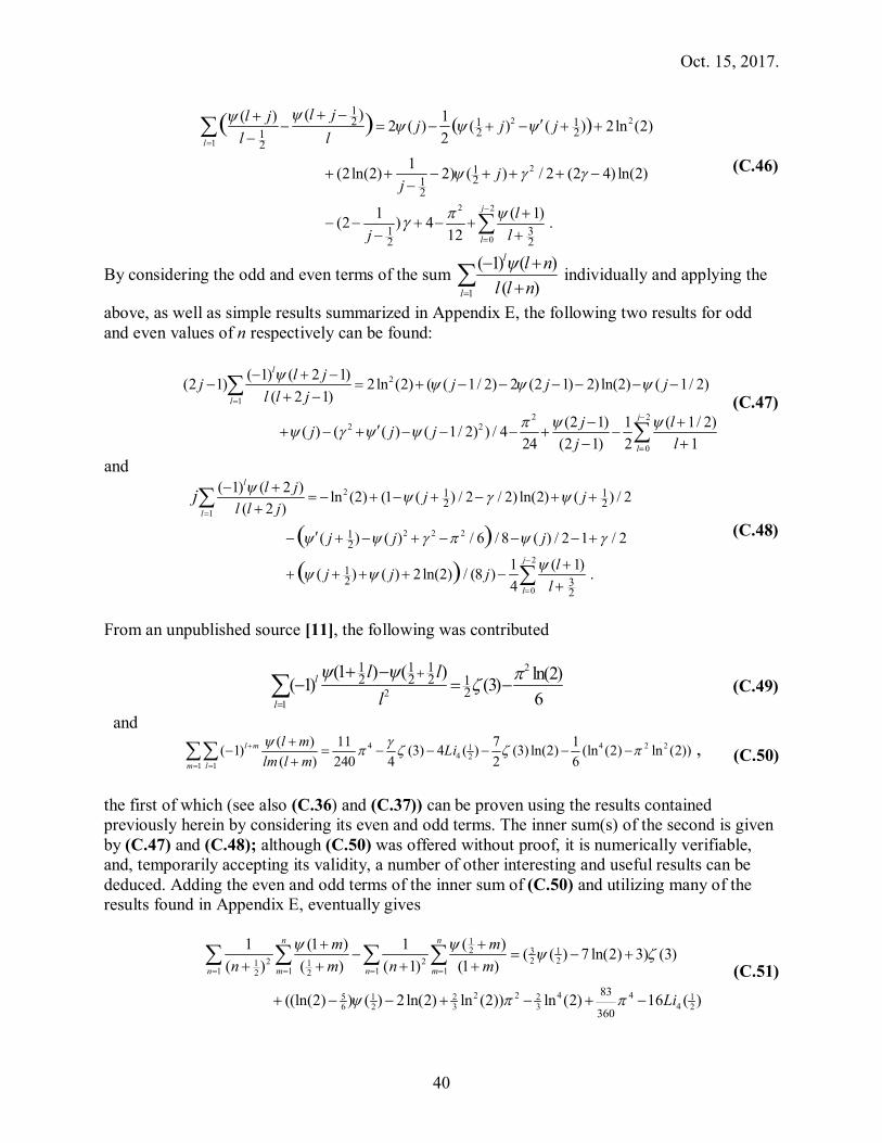
Oct. 15, 2017.
40
2 2
1
2
2 2
0
12 1 1
2 212
121
2
312 2
( )( ) 12 ( ) ( ) ( ) 2ln (2)2
1(2ln(2) 2) ( ) / 2 (2 4) ln(2)
1 ( 1)(2 ) 4 .12
( )( )l
j
l
l jl j j j jl l
jj
lj l
(C.46)
By considering the odd and even terms of the sum 1
( 1) ( )( )
l
l
l nl l n
individually and applying the
above, as well as simple results summarized in Appendix E, the following two results for odd and even values of n respectively can be found:
2
1
2 22 2
0
( 1) ( 2 1)(2 1) 2ln (2) ( ( 1/ 2) 2 (2 1) 2) ln(2) ( 1/ 2)( 2 1)
(2 1) 1 ( 1/ 2)( ) ( ( ) ( 1/ 2) ) / 424 (2 1) 2 1
l
l
j
l
l jj j j jl l j
j lj j jj l
(C.47)
and 2
1
2 2 2
2
0
1 12 2
12
12 3
2
( 1) ( 2 ) ln (2) (1 ( ) / 2 / 2) ln(2) ( ) / 2( 2 )
( ) ( ) / 6 / 8 ( ) / 2 1 / 2
1 ( 1)( ) ( ) 2 ln(2) / (8 ) .4
( )( )
l
l
j
l
l j j jl l j
j j j
lj j jl
j
(C.48)
From an unpublished source [11], the following was contributed
2
21
1 1 12 2 2 1
2(1 ) ( ) ln(2)( 1) (3)
6l
l
l ll
(C.49)
and 4 4 2 21
4 21 1
( ) 11 7 1( 1) (3) 4 ( ) (3) ln(2) (ln (2) ln (2))( ) 240 4 2 6
,l m
m l
l m Lilm l m
(C.50)
the first of which (see also (C.36) and (C.37)) can be proven using the results contained previously herein by considering its even and odd terms. The inner sum(s) of the second is given by (C.47) and (C.48); although (C.50) was offered without proof, it is numerically verifiable, and, temporarily accepting its validity, a number of other interesting and useful results can be deduced. Adding the even and odd terms of the inner sum of (C.50) and utilizing many of the results found in Appendix E, eventually gives
12 3 1
2 22 21 11 1 1 12 2
2 2 4 45 1 2 2 146 2 3 3 2
83
360
( )1 (1 ) 1 ( ( ) 7 ln(2) 3) (3)( ) ( ) ( 1) (1 )
((ln(2) ) ( ) 2 ln(2) ln (2)) ln (2) 16 ( )
n n
n m n m
mmn m n m
Li
(C.51)

Oct. 15, 2017.
41
or, after employing (23) 122 21 1
1 12 2
2 2 4 484 1 1 1 143 2 3 3 3 2
79
360
1 1 ( 1) (7 ( ) 7 ln(2)) (3)( ) ( 1) ( )
((ln(2) ) ( ) ln(2) ln (2)) ln (2) 8 ( ).
( )n
n m
mn n m
Li
(C.52)
Subtract (C.51) from (C.52) to obtain 12 1
22 11 1 2
2 2 4 41 1 2 1 1 1 142 2 3 3 3 90 2
112
( )1 ( 1) ( ( ) 14ln(2) 3) (3)( 1) (1 ) ( )
( ( ) ln(2) ln (2)) ln (2) 8 ( ) ,
( )n
n m
m mn m m
Li
(C.53)
Again apply (23) to the inner sum, and notice that all the sums so-created appear in Appendix E. After considerable computation and simplification, it is found that (C.53) reduces to an identity, thereby verifying (C.50). Alternatively, reorder (C.52) along a diagonal of the summation grid, interchange the summations, simplify using results from Appendix E and eventually obtain
4 4 21 12 121
1 22 2 21 1 1 1 1 1
42 2 2 2 12 2
7974 1440
514 2
( ) (2 1) ( ( ) ln(2) 1) (3) ln (2) 2ln (2) 5( )( (ln(2) ) 2 ln(2) ) ( ) ( ln(2) ln (2)) 2 ( ).
l
l ll
Li
(C.54)
Appendix D (A Special Case)
The following is the computer output defining the result associated with the generalization of (B.43) after differentiating with respect to the variable β. In the following, the variable B m and the various parameters
nY are defined following the main result. For the special cases m and 1m , see (B.45) and (B.46).

Oct. 15, 2017.
42
Appendix E (Simple Special Cases)
The following are commonly needed, useful and interesting cases that can be derived from the more general entries listed above, or extracted from the literature.
22
0
( 1 / 2) 7 (3) / 2( 1 / 2) 2l
ll
(E.1)*
2
20
( 1) ( 2ln(2)) 7 (3)( 1/ 2) 2l
ll
(E.2)
22
0
( 1) 1 (3)( 1) 6l
ll
(E.3)
4
30
( 1) (3)( 1) 360l
ll
(E.4) †
4
30
12
( 1) 7(2ln(2) ) (3)( ) 8l
ll
(E.5)
22
0
32 71
3 2( ) ( / 2 ln(2)) (3)
( 1)l
ll
(E.6)‡
012
( 1) 7 (3)( ) 2l
ll
(E.7)§
4 4 2 22
0
121
2
151 4 4ln (2) ln (2) 32 ( )360 3 3 4( 1)
28ln(2) (3)( )l
Lil
l
(E.8)
4
20
12
12
( ) 5( ) 24l
ll
(E.9)**
2 4 2 2
20
( 1) 11 2 (3)( 1) 360 6l
ll
(E.10)††
2
0
12
12
( ) 7ln(2) (3)( ) 2l
ll
(E.11) ‡‡
* Repeating footnote to (C.13). † See (72). ‡ Repeating (C.32). See also [9, Eq(15)]. § Repeating (C.25). **Special case of (C.31) ††See (72) and [9, Eq.(9)]. ‡‡ Repeating (C.13).

Oct. 15, 2017.
43
2 2 2
1
12
12
12
( )( 1) ( 2 ln(2)) / 3 /2 2 4 ln(2)( )l
lll l
(E.12)*
2 2
1
12
12
( ) ( 1) 2 (1 ln(2)) / 6 4 ln (2)( )l
l ll l
(E.13)†
2 4
2 20
12
12
( ) ( 1) 832ln(2)( 1) ( ) 3 12l
l ll l
(E.14)‡
2 2131
0 2
( 1) 4 ln(2) 4 ln (2)( 1)( )l
ll l
(E.15)
1
2 22 131
1 2
( ) 4( 2) ln(2) 8 ln (2) 4( )l
ll l
(E.16)§
2
0
12
( 1)( 1) ln (2) ln(2) .( 1)
l
l
ll
(E.17) 21
2
1
( 1) ( ) ln(2)( 2 ln(2)) .8
l
l
ll
(E.18)**
1
222
1
112
( ) 9( 1) (3)8
l
l
ll
(E.19)
142
21
17360
( )( 1) l
l
ll
(E.20)
The following are useful results extracted from [2], [7], [9], [10], [25] and/or [37]. From the general result [25, Eq. (3.11)] we have
22
1
5112 8
( 1)( 1) (3).l
l
ll
(E.21)
Quoting [9, Eq. (21)]
21
2 2 2 2 32 1 12 4
1
74
( ) (3) ln(2)( ) ( 4ln (2)) 4ln (2),l
ll
(E.22)
and from [25, Eq. (4.12)] or [7, Eq. (38)]
0
( 1) 2 (3) ,1l
ll
(E.23a)
2
0
1 14 4
( 1)( 1) (3) ln(2) ,1
l
l
ll
(E.23b)
along with, as a consequence of [10, Theorem 3.1] or (C.14),
* Special case of (C.43) † Special case of (C.44). ‡ See (E.8).E.8 § From [37], second unnumbered equation following (1.9), corrected for an incorrect exponent minus sign **See (C.37)

Oct. 15, 2017.
44
42
1.1
120( 1)
l
ll
(E.24)
From corrected [9, Eq. (22)], (apply a factor of two to the right-hand side; also see (E.6))
21
4 2 22 1 12 22
1
( ) / 8 ( ) / 6 7 ( ) (3).l
ll
(E.25)
Similarly, from the sixth (corrected) Example (3.6) of [37] – (remove the coefficient 72 ; it should
be unity) we obtain 2
4 2 2 2 4 22 1 4 143 2 3 221
1 2
61
360
(1 ) ( ln (2) 2 ln(2) ) ln (2) 14 (3) 4 32 ( ).( )l
l Lil
(E.26)
From corrected [9, Eq. (19)], (apply a minus sign to the right-hand side) or [25, Eq. (3.11) with k=2]
122 1
221
( )( 1) 7 (3)/2 2 ( ) /12.l
l
l Gl
(E.27)
From corrected [9, Eq. (12)], (replace ½ ζ(3) with ¼ ζ(3); also in [9, Eq. (11)] replace 2
12 with
2
12 ln(2) ), and (E.17) 2
3 2 2
0
1 13 4
(1 ) 2( 1) ln (2) ln (2) ( /12 )ln(2) (3).1
l
l
ll
(E.28)
From corrected [9, Eq. (8)], (to both Eq. (8) and previous unnumbered equation, replace
2112 ln(2) with 2 21
12 ln (2) ) or [7, Eq.(30)] we have
42 2 47
431
1 12 4 12
3112 4
( )( 1) 2 ( ) ln(2) (3) ln (2) ln (2) (3),48
l
l
l Lil
(E.29)
and from corrected [9, Eq. (13)], (contains the same error as [9, Eq. (8)] – see above)
24 4 2 21
421
12 4
1 (122
12( ) 11( 1) 2 ( ) ln (2) (7ln(2) ) (3) ln (2) ).
480l
l
l Lil
(E.30)
By considering the even and odd terms of (E.29) we obtain
1
2 2 4 42 1423
1
12
532 23 3 360
( ) (3)(14 ln(2) ( )) ln (2) ln (2) 16 ( )l
l Lil
(E.31)
and from the second unnumbered equation preceding [37, Eq. (1.5)] we have (see (11))
1
4 2 2 42 74 43
1
12
1 1 112 12120
( ) 2 ( ) ( ln(2)) (3) ln (2) ln (2).l
l Lil
(E.32)
By considering its even and odd terms, we also find

Oct. 15, 2017.
45
12 42 1
4 231
4 23 7 11 1 14 4 1440 12 12
( )( 1) ( ln(2)) (3) ln (2) ln (2) 2 ( ).l
l
l Lil
(E.33)
Extracted from [10, Section 8.2],
10 2
( )( 1) (1 / 2 ln(2)) 2( ) 4 2 ln(2)l
l
l Gl
(E.34)
and
4(3) 1431
0 2
3 3.71 ln(2)32 4 2 42
( 1)( 1) ( ) (3)( )
l
l
ll
(E.35)
where the trigamma function arises from [14] and the imaginary part of Li4(i). Also see (C.27) and C.28). By rewriting, and disentangling the remaining (corrected – also see (E.26)) cases presented in [37, Example (3.6)] (in the fifth case of this example collection, change the coefficient 41
16 to 6116 ) we find, after considerable effort, the following relations
1
222
1
58
16
( ) (3) ,l
ll
(E.36)
21
4 2 2 22 5 1 14 2 22
12 2 41
4212
1 26 3
1 16 120
12
( ) (3)(ln(2) ( )) ln (2) ln (2) ln(2) ( )
( ) 4 ( ) ,l
ll
Li
(E.37)
1
2 2 2 2 22 1 1 12 2 22
1
4 44
12
1 1 28 6 3
132
1724
124
( ) ( ) (3)(3 ( ) ln(2)) ( ) ln(2) ( ) ln (2)
ln (2) ( ) ,l
l ll
Li
(E.38)
2
212 2 2 22 1 1
2 2210 2
4 44
2
12
2323 360
43
( ) ( ) ( )(2 ln(2) 7 (3)) ln (2)( )
ln (2) 16 ( ) ,l
ll
Li
(E.39)
1
2 2 2 42 1 1 12 2 22
12 2 4
412
9 491 12 6 3 360
13
13
( ) ( ) (3) ( ) ( ) ln(2) ( )
ln (2) ln (2) 8 ( ) ,l
l ll
Li
(E.40)
1
2 2 2 42 1 1 12 2 221
1 22 2 4
412
4921 12 2 180
23
23
( ) ( ) (3) ( ) ( ) ln(2) ( )( )
ln (2) ln (2) 16 ( ),l
l ll
Li
(E.41)
and 1
2 2 4 42 14231
0 2
12
232 23 3 360
( ) 7 (3) ( ) ln (2) ln (2) 16 ( ).( )l
l Lil
(E.42)
Note that (E.42) is required for the proofs of (E.8), (E.31), (E.33), (E.40) and (E.41). Also, the separation of (E.38) into its even and odd components is required for the derivation of (E.40) and (E.41).

Oct. 15, 2017.
46
From [2, Eq. (3.71)] and [2, Eq. (3.93)], among many other sums expressed in terms of harmonic numbers, we find two interesting and representative results
26 4 2
21
101 122680 36
( 1) (3)( 1)l
ll
(E.43)
22 2
21
1214
2( ) ( 8 (3))
( )l
ll
(E.44)
Also, see (E.24) and (E.9). And finally, from [38] (in respective order: Eqs. (3.2a), (2.5c) – incorrect: the negative sign in the summand should be a plus sign – and (2.5d) – incorrect – the right-hand side should be preceded by a minus sign) we have, making use of (66) with n=4
22 2 4
31
71 16 2 36
( 1) ( ) (3) (5)l
ll
(E.45)
23
1
913 2
( 1) (3) (5)l
ll
(E.46)
and 2 4
21
7 713 2 360
( ) ( ) (3) (5) .l
l ll
(E.47)