ocean model predictions of chemistry changes from … · ocean model predictions of chemistry...

Ocean model predictions of chemistry changes from carbon dioxide

emissions to the atmosphere and ocean

Ken CaldeiraDepartment of Global Ecology, Carnegie Institution, Stanford, California, USA

Michael E. WickettCenter for Applied Computation Science, Lawrence Livermore National Laboratory, Livermore, California, USA

Received 17 August 2004; revised 9 March 2005; accepted 14 March 2005; published 21 September 2005.

[1] We present ocean chemistry calculations based on ocean general circulation modelsimulations of atmospheric CO2 emission, stabilization of atmospheric CO2 content, andstabilization of atmospheric CO2 achieved in total or in part by injection of CO2 to thedeep ocean interior. Our goal is to provide first-order results from various CO2 pathways,allowing correspondence with studies of marine biological effects of added CO2. Parts ofthe Southern Ocean become undersaturated with respect to aragonite under theIntergovernmental Panel on Climate Change Special Report on Emissions Scenarios(SRES) A1, A2, B1, and B2 emission pathways and the WRE pathways that stabilize CO2

at 650 ppm or above. Cumulative atmospheric emission of 5000 Pg C produces aragoniteundersaturation in most of the surface ocean; 10,000 Pg C also produces calciteundersaturation in most of the surface ocean. Stabilization of atmospheric CO2 at 450 ppmproduces both calcite and aragonite undersaturation in most of the deep ocean. Thesimulated SRES pathways produce global surface pH reductions of �0.3–0.5 units byyear 2100. Approximately this same reduction is produced by WRE650 and WRE1000stabilization scenarios and by the 1250 Pg C emission scenario by year 2300. Atmosphericemissions of 5000 Pg C and 20,000 Pg C produce global surface pH reductions of 0.8 and1.4 units, respectively, by year 2300. Simulations of deep ocean CO2 injection as analternative to atmospheric release show greater chemical impact on the deep ocean as theprice for having less impact on the surface ocean and climate. Changes in ocean chemistryof the magnitude shown are likely to be biologically significant.

Citation: Caldeira, K., and M. E. Wickett (2005), Ocean model predictions of chemistry changes from carbon dioxide emissions to

the atmosphere and ocean, J. Geophys. Res., 110, C09S04, doi:10.1029/2004JC002671.

1. Introduction

[2] Adding CO2 to the ocean, either passively or actively,affects the ocean carbonate system, resulting in decreasesin pH and carbonate-ion concentration [Zeebe and Wolf-Gladrow, 2001; Bolin and Eriksson, 1959]. These changeshave the potential to have strong impacts on marine biota[Kurihara et al., 2004; Portner et al., 2004; Langdon et al.,2003; Seibel and Walsh, 2001; Riebesell et al., 2000;Gattuso et al., 1999; Kleypas et al., 1999]. Here we predictocean chemistry changes for a range of cases of atmosphericCO2 emissions, atmospheric CO2 stabilization, and oceanCO2 injection using a stand-alone ocean general circulationmodel forced with changing carbon dioxide concentrationsor emissions, but no changing climate. The range of cases iswide enough such that it may span actual future atmosphericCO2 concentrations and emission rates, and thus couldprovide a context for marine biological studies relative toatmospheric CO2 emission or stabilization pathways.

[3] It has been suggested that continued release of CO2 tothe atmosphere may result in undersaturation of the surfaceocean with respect to the calcium carbonate minerals (i.e.,calcite and/or aragonite) and that this could potentiallyhave catastrophic biological consequences [Bacastow andKeeling, 1973; Fairhall, 1973; Broecker et al., 1971].Whitfield [1974] suggested this undersaturation would notoccur in the foreseeable future: a conclusion at odds withthe results presented here. Haugan and Drange [1996]compared paleo-pH, geographical and seasonal pH varia-tion, and projections from atmospheric invasion and directinjection cases. Brewer [1997] discussed ocean chemistrychanges that might occur to year 2100 under an Intergov-ernmental Panel on Climate Change (IPCC) ‘‘business-as-usual’’ pathway. Wolf-Gladrow et al. [1999] attempted apreliminary assessment of direct effects of anthropogenicCO2 increase on marine biota growth rates and carbonisotope fractionation. Kleypas et al. [1999] predictedchanges in calcification in corals to year 2100 under anIPCC business-as-usual pathway. Zondervan et al. [2001]looked at the consequences of anthropogenic CO2 forcalcification by marine plankton.

JOURNAL OF GEOPHYSICAL RESEARCH, VOL. 110, C09S04, doi:10.1029/2004JC002671, 2005

Copyright 2005 by the American Geophysical Union.0148-0227/05/2004JC002671$09.00

C09S04 1 of 12

[4] Aragonite and calcite are the two common CaCO3

mineral forms and are generally precipitated in the ocean inhighly saturated microenvironments created by marineorganisms. The degree of saturation of with respect toaragonite and calcite (WAragonite or WCalcite) is the ionproduct of the concentrations of calcium and carbonate ionsdivided by the stoichiometric solubility product [Feely etal., 2004]. Caldeira and Wickett [2003] compared estimatesof paleo-CO2 change with ocean pH anticipated under amulticentury 5000 Pg C (= 18,300 Pg CO2) atmosphericemission pathway. Feely et al. [2004] predicted aragoniteundersaturation for the entire ocean surface for this5000 Pg C emission pathway.[5] We performed several sets of simulations to look at

chemical effects of CO2 emission and stabilization pathways.Fromyear 2000 to 2100, we consider the single-century IPCCSpecial Report on Emissions Scenarios (SRES) A1, A2, B1,and B2 marker emission pathways [Intergovernmental Panelon Climate Change (IPCC), 2000] (available at http://www.grida.no/climate/ipcc/emission/index.htm). Fromyear 2000 to 2500, we consider the WRE450 throughWRE1000 atmospheric CO2 stabilization pathways [Wigleyet al., 1996] and a range of emission pathways withtotal cumulative future emissions ranging from 1250 to20,000 Pg C according to a smooth logistic curve [Marchetti,1991; Caldeira and Wickett, 2003].[6] We performed several simulations to look at chemical

effects of possible large-scale deployment of engineeredocean carbon storage [Herzog et al., 2001]. Many CO2

stabilization pathways (e.g., WRE550) require lower emis-sions than ‘‘business-as-usual’’ emission pathways. ThisCO2 emission avoidance can be attained through increasedefficiency, by carbon emission–free energy sources, or bysequestration of CO2 [Hoffert et al., 1998, 2002; Pacalaand Socolow, 2004]. We perform simulations in which all,10%, and none of this CO2 emission avoidance is accom-plished by directly injecting CO2 into the ocean. Thesesimulations show the chemical impact of this method ofemission avoidance and demonstrate, in principal, whetherthe method has the capacity to store the amount of CO2

needed to stabilize atmospheric CO2 under various assump-tions of atmospheric CO2 stabilization target and totalamount of ultimately recoverable fossil fuel resources.[7] Since the goal of this paper is to set out basic results

for a wide range of cases, we perform first-order calcula-tions without consideration of climate, circulation, marinebiological, land-biosphere, or dust feedbacks. Accuratelypredicting ocean chemistry involves accurately predictingclimate sensitivity, hydrological cycle, and wind changes,and the response of both the land biosphere and the ocean tosuch forcings. These factors could modify ocean chemistryin ways that are just beginning to be understood [e.g.,Sarmiento et al., 1998]. Here, we consider the changes inocean chemistry for up to a 500 year time period. On longertimescales, one would need to consider interactions with thecarbonate sedimentary system [Archer et al., 1997, 1998].[8] We would expect well-calibrated schematic model

results [e.g., Hoffert et al., 1979; Volker et al., 2002;Caldeira et al., 2002] to produce results similar to thespatially averaged results obtained from three-dimensionalmodels [e.g., Heinze, 2004; Orr et al., 2004; Caldeira andWickett, 2003]. However, the use of a three-dimensional

model allows for both better representation of physics andprediction of spatial variation. We would expect three-dimensional models run at higher, but still non-eddy-resolv-ing, resolutions to produce similar results on the scales thatwe resolve [Wickett et al., 2003].

2. Experimental Configuration

2.1. Ocean Model

[9] We use a configuration of the Lawrence LivermoreNational Laboratory (LLNL) ocean general circulationmodel [Caldeira and Wickett, 2003; Caldeira et al., 2002;Caldeira and Duffy, 2000] to predict future changes indissolved inorganic carbon (DIC) and then calculate theeffect of these changes on marine chemistry.[10] The model configuration is identical to that used by

Caldeira and Wickett [2003], with a global domain havinghorizontal resolution of 4� longitude by 2� latitude,24 levels in the vertical, and realistic but lightly smoothedtopography. Isopycnal and Gent-McWilliams diffusioncoefficients are 107 cm2 s�1. Vertical mixing is proportionalto the inverse of the Brunt-Vaisala frequency with a coef-ficient of 10�3 cm2 s�2, chosen to approximately recoverdeep North Pacific D

14C values. All surface forcings areobtained by linear interpolation in time between monthlymean climatological data. Wind forcing (i.e., momentumfluxes) is from an NCEP reanalysis [Kalnay et al., 1996].Surface salinities over open ocean are restored to Levitus etal. [1994] data with a time constant of 58 days. Under seaice, the sea ice model calculates fluxes of fresh water, andno restoring is used. Sensible, latent, longwave, and short-wave components of the surface heat flux are calculatedindependently using climatological atmospheric data, cal-culated sea surface temperatures, and bulk parameteriza-tions. The data and algorithms used in the heat fluxcalculations are described by Oberhuber [1993]. No restor-ing of sea surface temperature to prescribed values is used.[11] The model uses the abiotic carbon protocols from

the OCMIP-2 project (http://www.ipsl.jussieu.fr/OCMIP/phase2/simulations/Abiotic/HOWTO-Abiotic.html), underwhich ocean carbon is assumed to be a conservativetracer in the ocean interior and global ocean carboninventory is affected only by air-sea fluxes and directlyinjected carbon. The model was integrated for severalthousand years with preindustrial atmospheric forcing to anear-stationary state and was then integrated for theperiod 1750 to 2000 to achieve an initial state for thecases we present here. This model configuration takes up1.86 Pg C yr�1 for years 1980–1989 and 2.16 Pg C yr�1 foryears 1990–1999. This compares with 1.8 ± 0.8 Pg C yr�1

for years 1980–1989 and 1.9 ± 0.7 Pg C yr�1 for years1990–1999 estimated by Le Quere et al. [2003] and1.7 ± 0.6 Pg C yr�1 for years 1980–1989 and 2.4 ±0.7 Pg C yr�1 for years 1990–1999 estimated by Plattneret al. [2002].[12] Ocean carbon uptake and sequestration results for

configurations of this model have been presented by Orr etal. [2004], Caldeira and Wickett [2003], Wickett et al.[2003], Caldeira et al. [2002], and Caldeira and Duffy[2000]. In carbon sequestration simulations, our modelbehaves like a generic coarse-resolution z coordinate oceangeneral circulation model [Orr et al., 2004]. It simulates

C09S04 CALDEIRA AND WICKETT: OCEAN CHEMISTRY AND CO2 EMISSIONS

2 of 12

C09S04

tracers in the Southern Ocean [Caldeira and Duffy, 2000]fairly well and has reasonable predictions for global oceancarbon uptake in the 1980s and 1990s, but tends to get arelatively shallow North Atlantic thermohaline circulation,with much of the deep North Atlantic filling up withAntarctic Bottom Water. Nevertheless, it does a fairly goodjob of simulating the radiocarbon content of the deep NorthPacific [Caldeira et al., 2002], indicative of reasonableoverall ocean turnover rates.[13] To compute ocean chemistry, unless specified other-

wise, we use the chemistry routines from the OCMIP-3/NOCES project (http://www.ipsl.jussieu.fr/OCMIP/phase3/simulations/NOCES/HOWTO-NOCES.html). The originalversions of these routines were based on a code by Dickson[1994], but they have been modified by A. Mouchet andothers (J. Orr, personal communication, 2004). In all cases,we add changes predicted by the model to preindustrialconcentrations inferred from observations by the GLODAPproject [Key et al., 2004]. In reporting pH changes and otherresults, we report results relative to the preindustrial con-ditions (i.e., a pH change of 0.2 means a pH change of 0.2relative to the preindustrial concentrations inferred by Keyet al. [2004]).[14] The calculations performed here assume a neutral

biosphere. In the future, if the land-biosphere were to takeup significant amounts of carbon released to the atmo-sphere, atmospheric CO2 and ocean chemistry changeswould be less than predicted here (for emission cases) orallowable emissions would be greater than predicted here(for concentration stabilization cases).

2.2. Application of CO2 Boundary Conditions

[15] The model was configured to run cases of threetypes: (1) emission (specify CO2 emissions to the atmo-sphere, calculate atmospheric CO2 concentration); (2)stabilization (specify atmospheric CO2 concentration, cal-culate allowable CO2 emissions); and (3) deep oceaninjection (specify atmospheric CO2 concentration andCO2 emissions, calculate amount of emission avoidanceneeded to attain stabilization target; inject all or somefraction of this amount into the ocean interior).[16] The relations considered in these modes can be

summarized as follows:

Matm

d

dtxCO2ð Þ ¼ Fatm � Focean; ð1Þ

where Matm is the molar mass of the atmosphere, xCO2 isthe CO2 concentration in the atmosphere, Fatm is theemission to the atmosphere and Focean is the flux of CO2

from the atmosphere to the ocean. For emission cases (i.e.,SRES and logistic emission), Fatm is prescribed, the oceanmodel computes Focean, and atmospheric CO2 concentrationis predicted. For stabilization cases, atmospheric CO2

concentration is prescribed, the ocean model computesFocean, and Fatm is predicted.[17] For the deep ocean injection cases, we specify

both an emission pathway and a stabilization pathwayand define

Gap ¼ Femissionatm � Fstabilization

atm ; ð2Þ

where Fatmemission is the emission specified in the emission

pathway and Fatmstabilization is the amount allowed under the

stabilization pathway from equation (1). If Gap is positive,some fraction, k, is then injected to the ocean. Setting k tozero is equivalent to the stabilization cases. Experimentswith k equal to 1.0 have the property that total emissions(atmosphere plus ocean) are the same as in thecorresponding pure emission cases (e.g., 5000 Pg C overseveral centuries) but achieve the atmospheric stabilizationtargets of the stabilization cases (e.g., WRE550). We alsoperform experiments in which k is set to 0.1, whichassumes that 90% of the emission reduction is derivedfrom approaches other than direct injection of CO2 into theocean interior. Note that in these injection cases, Focean

from equation (1) includes any outgassing to the atmo-sphere of CO2 previously injected into the ocean.

3. Ocean Chemistry Consequences of Release ofCO2 to the Atmosphere

3.1. Emission Cases

[18] We consider two sets of emission pathways: cen-tury-scale SRES pathways and pathways that emit somespecified amount of CO2 over several centuries.3.1.1. Century-Scale SRES Pathways[19] The first set of cases (Figure 1b) is CO2 emissions

from the IPCC SRES A1, A2, B1, and B2 marker pathwaysfor years 2000 to 2100 [IPCC, 2000]. These CO2 emissionpathways were developed based on different assumptionsregarding global development over the rest of this century.The A1 storyline foresees rapid economic development inboth developing and developed countries with convergencebetween poor and rich countries. The A2 storyline has thelargest CO2 emissions, envisioning a world that has largeregional differences in rates of technological change, energytechnologies, approaches to agriculture, and access to min-eral resources. In contrast, the B1 storyline has the leastCO2 emissions, assuming a world with a globally coherentapproach to sustainable development with a high level ofenvironmental and social consciousness. The B2 world islike a less successful B1, with less technological advance-ment and greater regional differences in rates of develop-ment. The CO2 emissions in these pathways include netCO2 emissions from land use change.[20] We used the model to simulate 100 years for each

of the SRES pathways. Predicted atmospheric CO2 con-centrations are shown in Figure 1d and Table 1. Predictedchanges in surface ocean pH and calcite and aragonitesaturation state are shown in Figure 2 (horizontal means),and Figure 3 (zonal means). The lowest emission SRESpathway considered here (B1) produces global surface pHreductions of about 0.3 pH units by year 2100, whereasthe highest emission pathway considered (A2) producesglobal surface pH reductions approaching 0.5 pH units byyear 2100 (Figures 2 and 3). In our simulations, all of theSRES pathways produced aragonite undersaturation in thesurface Southern Ocean by year 2100 (Figure 3).3.1.2. Multicentury ‘‘Logistic’’ Emission Pathways[21] For the second set of emission pathways, we

develop a set of smooth CO2 emission curves releasingspecified amounts of CO2 to the atmosphere over the nextseveral centuries. In this set of emission pathways, start-


3 of 12

C09S04

ing in year 2000, CO2 emissions (dF/dt) and fossil fuelresources (F) are assumed to follow the logistic equation

dF

dt¼ aF tð Þ F 1750ð Þ � F tð Þ½ �: ð3Þ

We examine cases varying the value of the amount of CO2

emitted to the atmosphere after year 2000, F(2000). Weassume F(1750) = F(2000) + 270 Pg C (= 990 Pg CO2) (G.Marland et al., unpublished data, 2002) (available at http://cdiac.esd.ornl.gov/trends/emis/tre_glob.htm), and adjust a

Figure 1. (a) CO2 emissions scenarios releasing from 1250 to 20,000 Pg C (4580–73,300 Pg CO2) tothe atmosphere after year 2000 according to a smooth curve described by equation (3). (b) CO2 emissionsspecified for the Special Report on Emissions Scenarios (SRES) A1, A2, B1, and B2 pathways andallowable emissions calculated with our ocean model from WRE CO2 stabilization scenarios.(c) Atmospheric CO2 contents predicted by our model for the emission pathways shown in Figure 1a.(d) Atmospheric CO2 predicted for the SRES emission pathways and specified for the WRE stabilizationscenarios.

Table 1. Mean Surface Ocean Results for Simulated Years 2100 and 2300

Case Atmospheric CO2 Concentration, ppm Surface Ocean DpH WCalcite WAragonite

Preindustrial 280 . . . 5.2 3.4Year 2000 370 �0.09 4.4 2.9

IPCC SRES Pathways, Year 2100B2 820 �0.39 2.5 1.6A2 970 �0.46 2.1 1.4B1 650 �0.30 3.0 1.9A1 710 �0.34 2.8 1.8

‘‘Logistic’’ Pathways, Years 2100/23001250 Pg C 660/600 �0.31/�0.28 2.9/3.1 1.9/2.02500 Pg C 860/1020 �0.41/�0.49 2.4/2.0 1.5/1.35000 Pg C 1070/1980 �0.50/�0.77 2.0/1.1 1.3/0.710,000 Pg C 1240/4030 �0.56/�1.07 1.7/0.6 1.1/0.420,000 Pg C 1350/8110 �0.60/�1.37 1.6/0.3 1.0/0.2

Stabilization Pathways, Years 2100/2300WRE450 450/450 �0.17/�0.17 3.8/2.5 2.5/2.5WRE550 540/550 �0.23/�0.24 3.4/2.2 2.2/2.2WRE650 600/650 �0.27/�0.31 3.1/2.0 2.0/1.9WRE750 640/750 �0.29/�0.36 3.0/2.0 2.0/1.7WRE1000 680/990 �0.32/�0.47 2.9/1.9 1.9/1.4


4 of 12

C09S04

such that dF/dt = 6.8 Pg C in year 2000. The IPCC [2001]estimates global fossil fuel resources to be roughly5000 Pg C. Therefore we consider our base case to be5000 Pg C (= 18,300 Pg CO2) released to the atmosphere asCO2 over several centuries. Given that typically only half ofthe reduced carbon is recovered in fossil fuel miningoperations and there is a continuum of lower-grade carbon-rich shales, it is conceivable, given changing technologyand economics, eventual fossil fuel recovery on land couldreach 10,000 Pg C. Methane hydrates on continental shelveshave been estimated to contain another 10,000 Pg C; if thiswere recovered, then total amounts of fossil fuel carbonwould reach 20,000 Pg C. On the other hand, climateconcerns could result in diminished release of fossil fuelcarbon to the atmosphere, with the remainder of the fossilfuel resources permanently isolated from the atmosphere.Thus we examine cases in which from 1/4 to 4 timescurrently estimated fossil fuel carbon is released to theatmosphere as CO2 over the next several centuries. We referto these as ‘‘logistic’’ CO2 emission pathways.[22] Figure 1 shows the ‘‘logistic’’ CO2 emission path-

ways with integrated emissions after year 2000 rangingfrom 1250 to 20,000 Pg C. We used our ocean model tosimulate changes in ocean chemistry during 500 years ofemissions under these pathways. Emission of 1250 Pg Cproduces an average surface ocean pH decrease of nearly0.3 units by year 2300, whereas emission of 20,000 Pg Cdecreases surface pH by about 1.4 units. Emission of5000 Pg C according to this scenario decreases surfaceocean pH by about 0.8 pH units by 2300. Carbon absorbedby the ocean from the atmosphere initially affects the upperocean, but is then mixed down into the ocean interior.

Figure 2. (a) Surface ocean pH and (b) calcite (WCalcite)and aragonite (WAragonite) saturation state starting fromhorizontal mean observed concentrations [Key et al.,2004] with concentration changes applied from the three-dimensional ocean model simulations. Dashed lines showcalcite and aragonite saturation.

Figure 3. Predicted surface ocean pH change and calcite (WCalcite) and aragonite (WAragonite) saturationstate in (top) year 2100 for the SRES emission pathways and (bottom) year 2300 for the ‘‘logistic’’emission pathways. Preindustrial and year 2000 values are calculated from Key et al. [2004]. Chemistrychanges are computed from zonal mean average concentrations in the three-dimensional ocean model.Dashed lines show calcite and aragonite saturation.


5 of 12

C09S04

Because the pH of the upper thermocline is naturally lowerthan that of the surface waters, it is more sensitive to addedcarbon. Thus the greatest change in pH over the course ofthe simulation occurs several hundred meters below theocean surface (Figure 4), even though the highest anthro-pogenic carbon concentrations are at the surface.[23] By year 2300, the cases in which 10,000 Pg C and

20,000 Pg C are released to the atmosphere result inundersaturation of the surface ocean with respect to bothcalcite and aragonite. Emission of 1250 Pg C and 2500 Pg Cproduce surface waters that are saturated (on average) withrespect to calcite but undersaturated with respect to arago-nite (Figure 2). Emission of 5000 Pg C produces surfaceocean waters that are saturated with respect to aragoniteonly near the equator and undersaturated with respect tocalcite at high latitudes (Figure 3).[24] Today, horizontally averaged seawater composition

is saturated with respect to calcite from the surface of theocean to a depth greater than 3 km (Figure 5). In all of the‘‘logistic’’ emission cases considered here, the calcite lyso-cline shoals from deeper than 3 km to shallower than 1 km.For cases that cumulatively emit 2500 Pg C or more, the

calcite lysocline shoals to within a few hundred meters ofthe surface. In the transition, four layers can form from thetop to the bottom that alternate with respect to calcitesaturation, i.e., a surface layer that is calcite-saturatedoverlying a calcite-undersaturated layer in the thermocline,which in turn overlies a calcite-saturated layer centered atabout 1.5 km depth overlying an undersaturated deep ocean(Figure 5a; see, for example, the 1250 Pg C case at year2200).

3.2. Stabilization Cases

[25] Figure 1 shows the WRE450, WRE550, WRE650,WRE750, and WRE1000 atmospheric CO2 stabilizationpathways [Wigley et al., 1996]. These pathways aredesigned to follow a ‘‘business-as-usual’’ trajectory priorto transition to stable atmospheric CO2 concentrations. Weuse these pathways to address the question of oceanchemical consequences of atmospheric CO2 stabilization.[26] We used the model to simulate 500 years for each of

the WRE450 through WRE1000 stabilization pathways.Computed atmospheric CO2 emissions consistent with thesestabilization pathways are shown in Figure 1. Changes inocean pH and calcite and aragonite saturations states, basedon mean changes in surface ocean chemistry, are shown inFigure 2. On a global mean basis, the WRE650 pathwayproduces a surface ocean with a pH more than 0.3 unitslower than the preindustrial value. The WRE1000 pathwaydepresses surface ocean pH by about 0.5 pH units. On aglobal mean basis, surface waters remain saturated withrespect to both calcite and aragonite in these simulations.However, the Southern Ocean eventually becomes under-saturated with respect to aragonite in the Southern Oceanin the WRE650, WRE750, and WRE1000 simulations.Predicted changes in surface ocean pH and calcite and

Figure 4. Predicted horizontal mean ocean pH as afunction of depth and time for the ‘‘logistic’’ CO2 emissionpathways and WRE stabilization pathways. Chemistrychanges starting from Key et al. [2004] are computed fromhorizontal mean concentrations in the three-dimensionalocean model simulations.

Figure 5. Changes in the depth of the calcite lysocline for(a) ‘‘logistic’’ emission pathways and (b) WRE stabilizationpathways. The calcite lysocline represents the boundarybetween water that is saturated with respect to calcite andwater that is undersaturated with respect to calcite. Today,the upper ocean is calcite saturated. Chemistry changes,starting from Key et al. [2004], are calculated fromhorizontal mean concentrations in the three-dimensionalocean model simulation.


6 of 12

C09S04

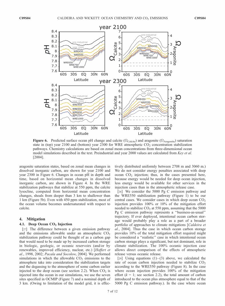
aragonite saturation states, based on zonal mean changes indissolved inorganic carbon, are shown for year 2100 andyear 2300 in Figure 6. Changes in ocean pH in depth andtime, based on horizontal mean changes in dissolvedinorganic carbon, are shown in Figure 4. In the WREstabilization pathways that stabilize at 550 ppm, the calcitelysocline, computed from horizontal mean concentrationchanges, shoals from deeper than 3 km to shallower than1 km (Figure 5b). Even with 450 ppm stabilization, most ofthe ocean volume becomes undersaturated with respect tocalcite.

4. Mitigation

4.1. Deep Ocean CO2 Injection

[27] The difference between a given emission pathwayand the emissions allowable under an atmospheric CO2

stabilization pathway could be thought of as a carbon gapthat would need to be made up by increased carbon storagein biologic, geologic, or oceanic reservoirs (and/or byrenewables, improved efficiency, nuclear, etc.) [Hoffert etal., 1998, 2002; Pacala and Socolow, 2004]. We performedsimulations in which the allowable CO2 emissions to theatmosphere take into consideration the stabilization targetsand the degassing to the atmosphere of some carbon earlierinjected to the deep ocean (see section 2.2). When CO2 isinjected into the ocean in our simulations, we use the sevensites specified in OCMIP (Figure 7) and a nominal depth of3 km. (Owing to limitation of the model grid, it is effec-

tively distributed uniformly between 2708 m and 3060 m.)We do not consider energy penalties associated with deepocean CO2 injection; thus, in the cases presented here,because energy would be needed for deep ocean injection,less energy would be available for other services in theinjection cases than in the atmospheric release case.[28] We consider the 5000 Pg C emission pathway and

the WRE550 stabilization pathway (Figure 1) to be ourcentral cases. We consider cases in which deep ocean CO2

injection provides 100% or 10% of the mitigation effortneeded to stabilize CO2 at 550 ppm, assuming that the 5000Pg C emission pathway represents a ‘‘business-as-usual’’trajectory. If ever deployed, intentional ocean carbon stor-age would probably play a role as a part of a broaderportfolio of approaches to climate mitigations [Caldeira etal., 2004]. Thus the case in which ocean carbon storageprovides 10% of the total mitigation effort required mightbe considered a ‘‘realistic’’ case in which intentional oceancarbon storage plays a significant, but not dominant, role inclimate stabilization. The 100% oceanic injection caseallows direct comparison of the effects of atmosphericrelease versus oceanic release.[29] Using equations (1)–(3) above, we calculated the

rate of ocean carbon injection needed to stabilize CO2

according to the WRE550 pathway (Figure 8). In the casewhere ocean injection provides 100% of the mitigationeffort (k = 1; see section 2.2), the total amount of carbonintroduced to the ocean plus atmosphere equal to that of the5000 Pg C emission pathway.). In the case where ocean

Figure 6. Predicted surface ocean pH change and calcite (WCalcite) and aragonite (WAragonite) saturationstate in (top) year 2100 and (bottom) year 2300 for WRE atmospheric CO2 concentration stabilizationpathways. Chemistry calculations are based on zonal mean concentrations from three-dimensional oceanmodel simulations described in the text. Preindustrial and year 2000 values are calculated from Key et al.[2004].


7 of 12

C09S04

injection provides 10% of the mitigation effort (k = 0.1), thetotal amount of carbon introduced to the ocean plus atmo-sphere is less that of the 5000 Pg C emission pathwaybecause other approaches are assumed to provide 90% ofthe required mitigation. In these cases, deep ocean injectionrates reach a maximum early in the 22nd century.[30] For the 100% deep ocean injection case, allowable

atmospheric emissions become negative by year 2200(Figure 8). This is because CO2 that had been injected intothe deep ocean is escaping to the atmosphere at a rate thatexceeds the atmospheric CO2 emission rate allowed underthe WRE550 stabilization pathway. This indicates that, evenin principal, direct injection of CO2 into the deep oceanwould not be able to provide 100% of the required mitiga-tion effort, but would need to be combined with someform of removal of CO2 from the atmosphere [Keith andHa-Duong, 2003]. In contrast, in the case where deep oceaninjection provides 10% of the mitigation effort, in year2500, atmospheric evasion of previously injected CO2 is0.3 Pg C yr�1, less than the 0.9 Pg C yr�1 allowed underthe WRE550 stabilization pathway. Thus degassing ofpreviously injected CO2 would diminish future CO2 emis-sions allowed from other sources, but would not requireactive removal of CO2 from the atmosphere.[31] Direct injection of CO2 into the ocean interior can

produce regions with higher dissolved inorganic carbonconcentrations than would occur with atmospheric release.CO2 injected into the ocean interior is retained in the poorlyventilated isopycnal layers of the deep ocean but is lost tothe atmosphere from the well-ventilated layers of the upperthermocline. Changes in ocean pH, based on horizontalmean ocean composition, are shown in Figure 9 for thecases described here. For the simulation in which deepocean injection provides 100% of the mitigation effort, deepocean pH values are much lower than in the WRE550simulation, however, surface ocean pH values are nearly thesame as in the WRE550 simulation.

[32] Volumes of water undergoing different changes inocean pH, for years 2100 and 2300, are shown if Figure 10.If ocean injection were to provide 10% of the total abate-ment required, by year 2100, on the order of 1% of theocean would have a large pH change relative to pH changesproduced by the WRE550 pathway; by year 2300, thissignal would spread out, so that most of the ocean would beroughly 0.1 pH unit lower than had the CO2 emissions beenabated without the use of the oceans. If ocean injection wereto provide 100% of the total abatement required, on theorder of 10% of the ocean would have a large pH changerelative to pH changes produced by the WRE550 pathway;by year 2300, this signal would spread out, and most of theocean would have a pH more than 0.5 unit lower than hadthe CO2 emissions been abated without the use of theoceans. Ocean CO2 injection could be engineered to dis-perse the carbon through a large range of depths in the deepocean, and this would reduce the maximum change inhorizontal mean ocean chemistry.

4.2. Dissolution of Carbonate Minerals

[33] It has been suggested [Kheshgi, 1995; Rau andCaldeira, 1999; Caldeira and Rau, 2000] that chemicaleffects of CO2 addition to the ocean could be mitigated bythe introduction of alkalinity to the oceans. Because of itsabundance, CaCO3 is the most likely source of thisalkalinity. Figure 11 shows how surface ocean pCO2,pH, and [COB3

2�] would change for different amounts ofadded CO2 and different amounts of dissolved CaCO3 perunit added CO2. It can be seen that the chemicalmitigation provided by the dissolution of carbonate min-erals is substantial, but partial. To maintain a constantcarbonate-ion concentration in a closed system, somewhatless than 1 mol CaCO3 would need to be added per molof CO2. To do this on a large scale implies massiveamounts of carbonate mineral [Rau and Caldeira, 1999].Furthermore, this would not completely mitigate the

Figure 7. Injection locations. Blue represents ocean seafloor deeper than 3 km [Smith and Sandwell,1997]. Colors on land represent distance to water deeper than 3 km. Coastal areas near deep water andCO2 sources likely would be preferred locations for direct injection of CO2 into the deep ocean.


8 of 12

C09S04

change in pH or pCO2. If enough CaCO3 were dissolvedto mitigate the change in pCO2, ocean pH and carbonate-ion concentrations would be higher than in their naturalstate. Nevertheless, addition of CaCO3 with CO2 bringsocean pCO2, pH, and [COB3

2�] closer to their naturalstate than they would be with the addition of CO2 alone.Thus there is potential to diminish chemical perturbationfrom added CO2, perhaps locally, through the dissolutionof carbonate minerals.

5. Discussion and Conclusions

[34] It is the goal of this study to allow a first-ordercorrespondence to be made between studies of marinebiological effects of added CO2 and various CO2 emissionsand stabilization pathways. A wide range of biologicalstudies suggests a sensitivity of marine biological systemsto added CO2 through a variety of mechanisms [e.g.,Kurihara et al., 2004; Portner et al., 2004; Langdon etal., 2003; Seibel and Walsh, 2001; Riebesell et al., 2000].[35] We have performed several sets of model simulations

to address two questions: (1) what changes in ocean

chemistry would be expected on the century and multi-century timescale for a range of atmospheric CO2 emissionand atmospheric CO2 stabilization pathways?; (2) whatchanges in ocean chemistry would be expected if directinjection of CO2 into the deep ocean were to be a significantcontributor to atmospheric CO2 stabilization?[36] Our simulations indicate that the SRES B1, A1, B2,

and A2 pathways all lead to aragonite undersaturation in thesurface Southern Ocean by year 2100. This is somewhatsurprising, since the B1 pathway is often looked upon as arelatively benign ‘‘spontaneous stabilization’’ pathway. TheWRE650, WRE750, and WRE1000 stabilization pathwayseventually produce aragonite undersaturation in all or partsof the Southern Ocean. The WRE550, WRE650, WRE750,and WRE1000 pathways result in the calcite lysoclineshoaling from a mean depth of greater than 3 km to a meandepth less than 1 km. Even relatively modest increases inatmospheric CO2 (e.g., to 450 ppm) cause the deep ocean to

Figure 8. Emissions and abatement associated withachieving WRE550 atmospheric CO2 stabilization startingfrom a 5000 Pg C (= 18,300 Pg CO2) atmospheric CO2

emission scenario: (a) emission to the atmosphere, (b)injection to the deep ocean, and (c) emissions abatementassumed to be provided by approaches other than directCO2 injection in the deep ocean. In each panel the black linerepresents a trajectory to emit 5000 Pg C of fossil fuelcarbon over several centuries according to a smooth logisticcurve described in the text; the green line representsemissions for CO2 stabilization at 550 ppm according to theWigley et al. [1995] pathway (this line is often hiddenbehind the blue line); the red line represents emissionschanges that would be needed if ocean injection made up100% of the carbon emissions avoidance; and the blue linerepresents emissions changes that would be needed if oceaninjection made up 10% of emission avoidance, with 90% ofavoidance coming from other means.

Figure 9. Changes in ocean pH predicted to occur if oceancarbon storage is used to stabilize CO2 according to theWRE550 stabilization trajectory given total CO2 emissionsfrom the ‘‘logistic’’ 5000 Pg C (= 18,300 Pg CO2) scenario.Ocean pH changes resulting from (a) atmospheric emissionof 5000 Pg C (see Figure 4); (b) WRE550 atmospheric CO2

pathway with injection at 3 km at 100% of the rate requiredto maintain total CO2 release rate equal to that in Figure 9a;(c) WRE550 atmospheric CO2 pathway with injection at3 km at 10% of the rate required to maintaining total CO2

release rate equal to that in Figure 9a; and (d) the WRE550atmospheric CO2 pathway (see Figure 4).


9 of 12

C09S04

make a transition from being predominately saturated withrespect to calcite to predominately undersaturated withrespect to calcite.[37] A pathway that releases 5000 Pg C (= estimated

fossil fuel resources) to the atmosphere over the next severalcenturies causes the ocean to become undersaturated withrespect to aragonite over nearly the entire surface. Iforganic-carbon rich shales or methane hydrates shouldprove minable, ultimate emissions could exceed 5000 Pg C.A pathway that emits 10,000 Pg C of CO2 to the atmosphereis predicted to produce surface ocean conditions that areundersaturated with respect to calcite nearly everywhere.Even if only one quarter of currently estimated fossilfuel resources are ultimately emitted to the atmosphere(= 1250 Pg C) as CO2, the ocean below 1 km is predictedto make a transition from being mostly saturated with respectto calcite to mostly undersaturated with respect to calcite.[38] The SRES pathways considered here produce global

surface pH reductions of about 0.3 to 0.5 pH units by year2100. This is roughly the same reduction as produced by theWRE650 and WRE1000 stabilization scenarios and by the1250 Pg C emission scenario by year 2300. Atmosphericemissions of 5000 Pg C and 20,000 Pg C produce globalsurface pH reductions of 0.8 and 1.4 pH units, respectivelyby year 2300.[39] For the simulation in which deep ocean injection

provides 100% of the mitigation effort, deep ocean pHvalues are much lower than in the WRE550 simulation;however, surface ocean pH values are nearly the same as inthe WRE550 simulation. There is potential to diminishchemical perturbation from added CO2, perhaps locally,through the dissolution of carbonate minerals.[40] In our simulations, the SRES B1 results are similar to

those of WRE750 and the SRES A1 results are similar tothat of WRE1000. Furthermore, the 1250 Pg C emissionscenario lies between the WRE550 and WRE650. Thissuggests that if we are to stabilize atmospheric CO2 attwice the preindustrial value, and use 5000 Pg C in fossilfuel resources, three quarters of that fossil fuel will need to

be used with carbon capture and storage. Atmosphericresults for the 2500 Pg C emission pathway are similar tothose from the WRE1000 stabilization pathway. Thusstabilization at 1000 ppm might require carbon captureand storage for roughly half of the carbon in remainingfossil fuel resources.[41] We did not simulate effects of changes in climate,

circulation, and marine biology. In the simulations ofSarmiento et al. [1998], these feedbacks produced second-order effects on carbon uptake. Carbonate dissolutioneffects are thought to be small on the timescales consideredhere [Heinze, 2004; Zondervan et al., 2001; Archer et al.,1997, 1998], but would operate to lessen the magnitude ofour results. We conjecture, but have not proved, thatconsideration of these feedbacks would produce second-order modifications to our basic results.[42] Using a 5000 Pg C emission pathway and a 550 ppm

atmospheric stabilization target, our simulations indicatethat injection of CO2 into the deep ocean alone could notfill the entire carbon emission–free energy gap in theabsence of CO2 removal from air. After several centuriesof deep sea injection, the flux of previously injected carbondioxide degassing to the atmosphere would exceed the totalallowable CO2 emissions under the stabilization pathway.Without atmospheric removal, atmospheric CO2 contentwould increase. In contrast, when ocean injection fills10% of the CO2 emission avoidance ‘‘gap,’’ degassing ofinjected carbon is generally far slower than the CO2

emission rate allowed under the stabilization pathway. So,from the point of view of effectiveness of storage, oceaninjection could potentially solve 10% of the problem, butcould not solve 100% of the problem in the absence ofactive CO2 removal from air several centuries into thefuture. Deep ocean CO2 injection as an alternative toatmospheric release makes a greater chemical impact onthe deep ocean as the price for having less of an impact onthe surface ocean and climate.[43] Our results indicate that atmospheric release of

CO2 will produce changes in ocean chemistry that could

Figure 10. Fraction of ocean volume (between 60�N and 60�S) with a pH change greater than somespecified amount in (a) year 2100 and (b) year 2300 for the cases shown in Figures 8 and 9. Lines are asfollows: ‘‘5000 Pg C’’ shows predicted pH consequences of releasing 5000 Pg C of fossil fuel carbon tothe atmosphere over several centuries according to a smooth curve described in the text; ‘‘WRE550’’shows ocean pH changes predicted to result from CO2 stabilization at 550 ppm according to the WRE550pathway; ‘‘100%’’ shows ocean pH changes that would be expected if ocean injection made up 100% ofthe carbon emissions avoidance; and ‘‘10%’’ shows ocean pH changes that would be expected if oceaninjection made up 10% of emission avoidance, with 90% of avoidance coming from other means.


10 of 12

C09S04

affect marine ecosystems significantly, even under futurepathways in which most of the remaining fossil fuel CO2

is never released. Thus chemical effects of CO2 on themarine environment may be as great a cause for concernas the radiative effects of CO2 on Earth’s climate.

[44] Acknowledgments. We wish to thank Ed Urban of the ScientificCommittee on Oceanic Research (SCOR) and Maria Hood of the Intergov-ernmental Oceanographic Commission (IOC) of UNESCO for their effortsto bring attention to the issue of ocean chemistry changes. This researchwas supported by the DOE Office of Science Office of Biological andEnvironmental Research Ocean Carbon Sequestration Research Program.This work was performed under the auspices of the U.S. Department of

Energy by University of California Lawrence Livermore National Labora-tory under contract W-7405-Eng-48.

ReferencesArcher, D., H. Kheshgi, and E. Maier-Reimer (1997), Multiple timescalesfor neutralization of fossil fuel CO2, Geophys. Res. Lett., 24, 405–408.

Archer, D., H. Kheshgi, and E. Maier-Reimer (1998), Dynamics of fossilfuel neutralization by marine CaCO3, Global Biogeochem. Cycles, 12,259–276.

Bacastow, R., and C. D. Keeling (1973), Atmospheric carbon dioxide andradio-carbon in the natural carbon cycle. II: Changes from A. D. 1700 to2070 as deduced from a geochemical model, in Carbon in the Biosphere,AEC Symp. Ser., vol. 30, edited by G. M. Woodwell and E. V. Pecan,pp. 86–136, NTIS U. S. Dep. of Commerce, Springfield, Va.

Bolin, B., and E. Eriksson (1959), Changes in the carbon dioxide content ofthe atmosphere and the sea due to fossil fuel combustion, in The Atmo-sphere and the Sea in Motion, pp. 130–142, Rockefeller Inst. Press, NewYork.

Brewer, P. G. (1997), Ocean chemistry of the fossil fuel CO2 signal: Thehaline signal of ‘‘business as usual,’’ Geophys. Res. Lett., 24, 1367–1369.

Broecker, W. S., Y.-H. Li, and T.-H. Peng (1971), Carbon dioxide: Man’sunseen artifact, in Impingement of Man on the Oceans, edited by D. W.Hood, pp. 287–324, Wiley Intersci., Hoboken, N. J.

Caldeira, K., and P. B. Duffy (2000), The role of the Southern Ocean inuptake and storage of anthropogenic carbon dioxide, Science, 287, 620–622.

Caldeira, K., and G. H. Rau (2000), Accelerating carbonate dissolution tosequester carbon dioxide in the ocean: Geochemical implications, Geo-phys. Res. Lett., 27, 225–228.

Caldeira, K., and M. E. Wickett (2003), Anthropogenic carbon and oceanpH, Nature, 425, 365–365.

Caldeira, K., M. E. Wickett, and P. B. Duffy (2002), Depth, radiocarbon,and the effectiveness of direct CO2 injection as an ocean carbon seques-tration strategy, Geophys. Res. Lett., 29(16), 1766, doi:10.1029/2001GL014234.

Caldeira, K., G. Morgan, D. Baldocchi, P. Brewer, C. T. A. Chen, G.-J.Nabuurs, N. Nakicenovic, and G. P. Robertson (2004), A portfolio ofcarbon management options, in The Global Carbon Cycle: IntegratingHumans, Climate, and the Natural World, SCOPE, vol. 62, edited byC. B. Field, pp. 103–130, Island Press, Washington, D. C.

Dickson, A. (1994), Handbook of Methods for the Analysis of the VariousParameters of the Carbon Dioxide System in Seawater, SOP 3, pp. 25–26, U.S. Dep. of Energy, Washington, D. C.

Fairhall, A. W. (1973), Accumulation of fossil CO2 in the atmosphere andthe sea, Nature, 245, 20–23.

Feely, R. A., C. L. Sabine, K. Lee, W. Berelson, J. Kleypas, V. J. Fabry, andF. J. Millero (2004), Impact of anthropogenic CO2 on the CaCO3 systemin the oceans, Science, 305, 362–366.

Gattuso, J.-P., D. Allemand, and M. Frankignoulle (1999), Interactionsbetween the carbon and carbonate cycles at organism and communitylevels in coral reefs: A review on processes, rates and environmentalcontrol, Am. Zool., 39, 160–183.

Haugan, P. M., and H. Drange (1996), Effects of CO2 on the ocean envir-onment, Energy Convers. Manage., 37, 1019–1022.

Heinze, C. (2004), Simulating oceanic CaCO3 export production in thegreenhouse, Geophys. Res. Lett. , 31 , L16308, doi:10.1029/2004GL020613.

Herzog, H., K. Caldeira, and E. Adams (2001), Carbon sequestration viadirect injection, in Encyclopedia of Ocean Sciences, vol. 1, edited by J. H.Steele, S. A. Thorpe, and K. K. Turekian, pp. 408–414, Elsevier, NewYork.

Hoffert, M. I., Y.-C. Wey, A. J. Callegari, and W. S. Broecker (1979),Atmospheric response to deep-sea injections of fossil-fuel carbon diox-ide, Clim. Change, 2, 53–68.

Hoffert, M. I., et al. (1998), Energy implications of future stabilization ofatmospheric CO2 content, Nature, 395, 881–884.

Hoffert, M. I., et al. (2002), Advanced technology paths to global climatestability: Energy for a greenhouse planet, Science, 295, 981–987.

Intergovernmental Panel on Climatic Change (IPCC) (2000), SpecialReport on Emissions Scenarios, Working Group III, IntergovernmentalPanel on Climate Change, edited by N. Nakicenovic et al., 595 pp.,Cambridge Univ. Press, New York.

Intergovernmental Panel on Climatic Change (IPCC) (2001), Third Assess-ment Report of Working Group III, Mitigation, edited by B. Metz et al.,752 pp., Cambridge Univ. Press, New York.

Kalnay, E., et al. (1996), The NCEP/NCAR 40-year reanalysis project, Bull.Am. Meteorol. Soc., 77, 437–471.

Keith, D. W., and M. Ha-Duong (2003), CO2 capture from the air: Tech-nology assessment and implications for climate policy, in Proceedings of

Figure 11. Effects of adding CO2 and dissolved CaCO3 onmean surface ocean chemistry, assuming uniform distribu-tion in the ocean. CaCO3 dissolution can mitigate much, butnot all, of the chemical effects of CO2 addition. The dashedlines indicate no change in the chemical parameter (pCO2,pH, or [CO3

2�]). For example, a uniform addition of2000 Pg C as CO2 and 8800 Pg CaCO3 to a preindustrialocean with a pCO2 of 280 matm (molar ratio = 1.2) wouldproduce roughly 340 matm pCO2, almost no change in pH,and a carbonate-ion concentration roughly 20 mmol kg�1

higher than present.


11 of 12

C09S04

the 6th Greenhouse Gas Control Conference, Kyoto, Japan, edited byJ. Gale and Y. Kaya, pp. 187–197, Elsevier, New York.

Key, R. M., A. Kozyr, C. L. Sabine, K. Lee, R. Wanninkhof, J. L. Bullister,R. A. Feely, F. Millero, C. Mordy, and T.-H. Peng (2004), A global oceancarbon climatology: Results from Global Data Analysis Project(GLODAP), Global Biogeochem. Cycles, 18, GB4031, doi:10.1029/2004GB002247.

Kheshgi, H. S. (1995), Sequestering atmospheric carbon dioxide by increas-ing ocean alkalinity, Energy Int. J., 20, 915–922.

Kleypas, J. A., R. W. Buddemeier, D. Archer, J.-P. Gattuso, C. Langdon,and B. N. Opdyke (1999), Geochemical consequences of increased atmo-spheric CO2 on coral reefs, Science, 284, 118–120.

Kurihara, H., S. Shimode, and Y. Shirayama (2004), Sub-lethal effects ofelevated concentration of CO2 on planktonic copepods and sea urchins,J. Oceanogr., 60, 743–750.

Langdon, C., W. S. Broecker, D. E. Hammond, E. Glenn, K. Fitzsimmons,S. G. Nelson, T.-S. Peng, I. Hajdas, and G. Bonani (2003), Effectof elevated CO2 on the community metabolism of an experimentalcoral reef, Global Biogeochem. Cycles, 17(1), 1011, doi:10.1029/2002GB001941.

Le Quere, C., et al. (2003), Two decades of ocean CO2 sink and variability,Tellus, Ser. B, 55, 649–656.

Levitus, S., R. Burgett, and T. P. Boyer (1994), World Ocean Atlas 1994,vol. 3, Salinity, NOAA Atlas NESDIS 3, 111 pp., Natl. Oceanic andAtmos. Admin., Silver Spring, Md.

Marchetti, C. (1991), Branching out into the universe, in Diffusion of Tech-nologies and Social Behavior, edited by N. Nakicenovic and A. Grubler,pp. 583–592, Springer, New York.

Oberhuber, J. M. (1993), Simulation of the Atlantic circulation with acoupled sea-ice mixed layer-isopycnal general circulation model. Part I:Model description, J. Phys. Oceanogr., 13, 808–829.

Orr, J. C., et al. (2004), Narrowing the uncertainty for deep ocean injectionefficiency, in Proceedings of the 7th International Conference on Green-house Gas Control Technologies, edited by E. S. Rubin, D. W. Keith, andC. F. Gilboy, IEA Greenhouse Gas Prog., Vancouver, B. C., Canada.

Pacala, S., and R. Socolow (2004), Stabilization wedges: Solving the cli-mate problem for the next 50 years with current technologies, Science,305, 968–972.

Plattner, G.-K., F. Joos, and T. F. Stocker (2002), Revision of the globalcarbon budget due to changing air-sea oxygen fluxes, Global Biogeo-chem. Cycles, 16(4), 1096, doi:10.1029/2001GB001746.

Portner, H. O., M. Langenbuch, and A. Reipschlager (2004), Biologicalimpact of elevated ocean CO2 concentrations: Lessons from animalphysiology and earth history?, J. Oceanogr., 60, 705–718.

Rau, G. H., and K. Caldeira (1999), Enhanced carbonate dissolution: Ameans of sequestering waste CO2 as ocean bicarbonate, Energy Conver.Manage., 40, 1803–1813.

Riebesell, U., I. Zondervan, B. Rost, P. D. Tortell, R. E. Zeebe, and F. M.M. Morel (2000), Reduced calcification of marine plankton in response toincreased atmospheric CO2, Nature, 407, 364–367.

Sarmiento, J. L., T. M. C. Hughes, R. J. Stouffer, and S. Manabe (1998),Simulated response of the ocean carbon cycle to anthropogenic climatewarming, Nature, 393, 245–249.

Seibel, B. A., and P. J. Walsh (2001), Potential impacts of CO2 injections ondeep-sea biota, Science, 294, 319–320.

Smith, W. H. F., and D. T. Sandwell (1997), Global seafloor topographyfrom satellite altimetry and ship depth soundings, Science, 277, 1957–1962.

Volker, C., D. W. R. Wallace, and D. A. Wolf-Gladrow (2002), On therole of heat fluxes in the uptake of anthropogenic carbon in the NorthAtlantic, Global Biogeochem. Cycles, 16(4), 1138, doi:10.1029/2002GB001897.

Whitfield, M. (1974), Accumulation of fossil CO2 in the atmosphere andthe sea, Nature, 247, 523–525.

Wickett, M. E., K. Caldeira, and P. B. Duffy (2003), Effect of horizontalgrid resolution on simulations of oceanic CFC-11 uptake and direct in-jection of anthropogenic CO2, J. Geophys. Res., 108(C6), 3189,doi:10.1029/2001JC001130.

Wigley, T., R. Richels, and J. Edmonds (1996), Economic and environ-mental choices in the stabilization of atmospheric CO2 concentration,Nature, 379, 242–245.

Wolf-Gladrow, D. A., U. Riebesell, S. Burkhardt, and J. Bijma (1999),Direct effects of CO2 concentration on growth and isotopic compositionof marine plankton, Tellus, Ser. B, 51, 461–476.

Zeebe, R. E., and D. A. Wolf-Gladrow (2001), Seawater: Equilibrium,Kinetics, Isotopes, Elsevier Oceanogr. Ser., vol. 65, Elsevier, New York.

Zondervan, I., R. E. Zeebe, B. Rost, and U. Riebesell (2001), Decreasingmarine biogenic calcification: A negative feedback on rising atmosphericpCO2, Global Biogeochem. Cycles, 15, 507–516.

��K. Caldeira, Department of Global Ecology, Carnegie Institution, 260

Panama Street, Stanford, CA 94305, USA. ([email protected])M. E. Wickett, Center for Applied Computation Science, Lawrence

Livermore National Laboratory, 7000 East Avenue, L-103, Livermore, CA94550, USA. ([email protected])


12 of 12

C09S04

ocean model predictions of chemistry changes from … · ocean model predictions of chemistry...

Documents