ocean city md ngdc dem - university of delaware inundation mapping for ocean city, md ngdc dem by...
TRANSCRIPT
TSUNAMI INUNDATION MAPPING FOR
OCEAN CITY, MD NGDC DEM
BY
BABAK TEHRANIRAD, SAEIDEH BANIHASHEMI,
JAMES T. KIRBY, JOHN A. CALLAHAN AND
FENGYAN SHI
RESEARCH REPORT NO. CACR-14-04
NOVEMBER 2014
SUPPORTED BY THE NATIONAL TSUNAMI HAZARD MITIGATION PROGRAM
NATIONAL WEATHER SERVICE GRANT NA10NWS4670010
CENTER FOR APPLIED COASTAL RESEARCH
Ocean Engineering Laboratory
University of Delaware
Newark, Delaware 19716
Tsunami Inundation Mapping for Ocean City, MD NGDC DEM
BY
Babak Tehranirad1, Saeideh Banihashemi
1,
James T. Kirby1, John A. Callahan
2 and
Fengyan Shi1
1Center for Applied Coastal Research, Department of Civil and
Environmental Engineering, University of Delaware,
Newark, DE 19716, USA
2Delaware Geological Survey, University of Delaware,
Newark, DE 19716, USA
Abstract
This document reports the development of tsunami inundation maps for the re-
gion covered by the NGDC tsunami DEM for Ocean City, MD. Section 1 describes
NTHMP requirements and guidelines for this work. The location of the study and the
bathymetry data utilized are described. Tsunami sources that potentially threaten the
upper East Coast of the United States are briefly discussed. Modeling inputs are de-
scribed in the Section 3, including model specifications and simulation methods such
as nesting approaches used in generating inundation maps. The process of generating
inundation maps from tsunami simulation results is described in Section 4, along with
other results such as arrival time of the tsunami. GIS data sets and organization, in-
cluding inundation maps, maximum velocity maps, maximum momentum flux maps,
are described in Appendix A. Modeling inputs for simulation are provided in Ap-
pendix B for interested modelers. In Appendix C, NTHMP guidelines for inundation
mapping are provided.
i
Contents
1 Introduction 1
2 Background Information about Map Area 1
2.1 Location of coverage, and communities covered . . . . . . . . . . . . . . 1
2.2 Tsunami sources . . . . . . . . . . . . . . . . . . . . . . . . . . . . . . 2
2.2.1 Coseismic sources . . . . . . . . . . . . . . . . . . . . . . . . . 4
2.2.2 Volcanic cone collapse . . . . . . . . . . . . . . . . . . . . . . . 4
2.2.3 Submarine mass failure . . . . . . . . . . . . . . . . . . . . . . . 5
3 Modeling Inputs 6
3.1 Numerical model . . . . . . . . . . . . . . . . . . . . . . . . . . . . . . 6
3.2 Bathymetric Input Data . . . . . . . . . . . . . . . . . . . . . . . . . . . 7
3.2.1 Ocean City NGDC DEM . . . . . . . . . . . . . . . . . . . . . . 7
3.2.2 NGDC Coastal Relief Model (CRM) . . . . . . . . . . . . . . . 8
3.2.3 ETOPO 1 . . . . . . . . . . . . . . . . . . . . . . . . . . . . . . 8
3.3 Model Grids . . . . . . . . . . . . . . . . . . . . . . . . . . . . . . . . . 9
3.4 Nesting approach . . . . . . . . . . . . . . . . . . . . . . . . . . . . . . 10
4 Results 17
4.1 Arrival time . . . . . . . . . . . . . . . . . . . . . . . . . . . . . . . . . 18
4.2 Raster Data . . . . . . . . . . . . . . . . . . . . . . . . . . . . . . . . . 20
4.3 Inundation line . . . . . . . . . . . . . . . . . . . . . . . . . . . . . . . 27
ii
5 Map Construction 31
A Gridded Data Information A–1
B Modeling inputs B–1
C Inundation Mapping Guidelines C–1
iii
List of Figures
1 Location of the NGDC Ocean City DEM (Grothe et al, 2010). Color bar
shows depth values in meters for areas inside of the DEM boundary. . . . 3
2 Locations of the Grids used in this project and also the center of SMF
sources simulated here. . . . . . . . . . . . . . . . . . . . . . . . . . . . 11
3 Location of Grid B and Ocean City DEM used in this project, and also the
initial stage of SMF sources. . . . . . . . . . . . . . . . . . . . . . . . . 12
4 Gauge data at the southeastern edge of Grid A for coseismic and volcanic
collapse sources . . . . . . . . . . . . . . . . . . . . . . . . . . . . . . . 14
5 This figure demonstrates the nesting approach diagram. The figure on the
top left depicts the Grid A and B as well as the location of the Ocean City
DEM. The figure on the right show the 1 arc-sec grids described in Table
??. Also, in the bottom left figure the 1/3 arc-sec domains are shown (Also
described in Table ??). . . . . . . . . . . . . . . . . . . . . . . . . . . . 16
6 Recorded Surface Elevation for NOAA Gauges which are located in Ocean
City DEM, Ocean City (Green), Cape Henlopen (Red), and Lewes (Blue) 19
7 SMF4 Inundation Map for the Ocean City DEM with 4 arc-second resolu-
tion. Red squares depicts the 1 arc-second resolution domains . . . . . . 22
8 Inundation depth for OC 1arc 1 domain, A) SMF Envelope, B) Coseismic
Envelope, C) CVV 80 km3 slide, and D) CVV 450 km3 slide. Red box
depicts OC 1arc 1 domain boundaries. . . . . . . . . . . . . . . . . . . . 23
iv
9 Inundation depth for OC 1arc 2 domain, A) SMF Envelope, B) Coseismic
Envelope, C) CVV 80 km3 slide, and D) CVV 450 km3 slide. Red box
depicts OC 1arc 2 domain boundaries. . . . . . . . . . . . . . . . . . . . 24
10 Inundation depth for OC 1arc 3 domain, A) SMF Envelope, B) Coseismic
Envelope, C) CVV 80 km3 slide, and D) CVV 450 km3 slide. Red box
depicts OC 1arc 3 domain boundaries. . . . . . . . . . . . . . . . . . . . 25
11 Inundation depth for OC 1arc 4 domain, A) SMF Envelope, B) Coseismic
Envelope, C) CVV 80 km3 slide, and D) CVV 450 km3 slide. Red box
depicts OC 1arc 4 domain boundaries. . . . . . . . . . . . . . . . . . . . 26
12 (Maximum Momentum Flux Map for Bethany Beach domain (1/3 Arc-
sec) during SMF4 tsunami (Colorbar values are in m3/s2) . . . . . . . . 28
13 (a) Maximum Velocity map for inundated area around Indian River Inlet
(SMF4) (b) Maximum Velocity map for Indian River Inlet for offshore
areas (SMF4) . . . . . . . . . . . . . . . . . . . . . . . . . . . . . . . . 29
14 Maximum Vorticity map for the area around Ocean City inlet . . . . . . . 30
15 Tsunami inundation Line for Ocean City NGDC DEM area based on tsunami
sources simulated in this project. The blue boxes show the location of the
inundation maps discussed in Section 5. . . . . . . . . . . . . . . . . . . 32
16 Inundation map for emergency planning for Lewes and Rehoboth Beach,
DE in 1:30,000 scale. The inundated area is covered in red, and the thick
red line represents the inundation line for this particular area. . . . . . . . 34
v
17 Inundation map for emergency planning for Bethany Beach and Fenwick
Island, DE in 1:30,000 scale. The inundated area is shown in red, and the
thick red line represents the inundation line for this particular area. . . . . 35
18 Inundation map for emergency planning for Ocean City, MD at 1:30,000
scale. The inundated area is covered in red, and the thick red line repre-
sents the inundation line for this particular area. . . . . . . . . . . . . . . 36
19 Inundation map for emergency planning for Chincoteague, VA at 1:40,000
scale. The inundated area is covered in red, and the thick red line repre-
sents the inundation line for this particular area. . . . . . . . . . . . . . . 37
20 Screen shot of the results folder . . . . . . . . . . . . . . . . . . . . . . . A–4
21 Screen shot of the input folder . . . . . . . . . . . . . . . . . . . . . . . B–2
vi
List of Tables
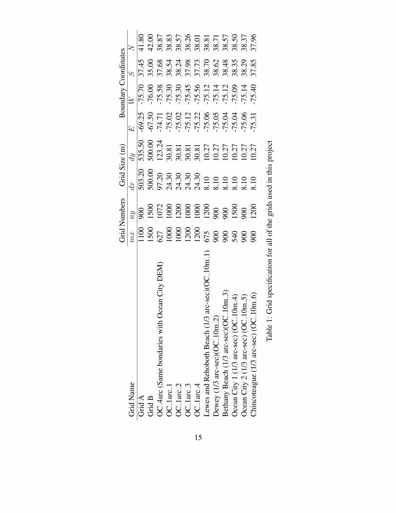
1 Grid specification for all of the grids used in this project . . . . . . . . . . 15
2 Arrival time in minutes after tsunami initiation for different locations and
sources in Ocean City DEM based on the location of NOAA gauges.
CVV1 and CVV2 refer to 80 km3 and 450 km3 slide volumes respectively. 20
vii
1 Introduction
The US National Tsunami Hazard Mitigation Program (NTHMP) supports the develop-
ment of inundation maps for all US coastal areas through numerical modeling of tsunami
inundation. This includes high-resolution modeling and mapping of at-risk and highly
populated areas as well as the development of inundation estimates for non-modeled and
low hazard areas. This report describes the development of inundation maps for a region
covered by the Ocean City NGDC tsunami DEM (Grothe et al, 2010).
In section 2, background information about the mapped area is provided. Possible
tsunami sources that threaten the upper United States East Coast (USEC), and are consid-
ered in this analysis, are described. Modeling inputs are described in section 3. Section
4 presents simulation results and the development of mapping products. The process of
obtaining the tsunami inundation line, which is the most significant result of this work,
is explained in this section. Three appendices provide information about GIS data stor-
age and content (Appendix A), modeling inputs (Appendix B), and NTHMP inundation
mapping guidelines (Appendix C).
2 Background Information about Map Area
2.1 Location of coverage, and communities covered
The National Oceanic and Atmospheric Administration (NOAA), National Geophysical
Data Center (NGDC) have generated digital elevation models (DEM) as input for studies
focusing on hazard assessment of catastrophes like tsunamis and hurricanes at a number
1

of U. S. coastal areas. The Ocean City NGDC DEM covers a portion of the mid-Atlantic
coastline including Delaware, Maryland, and the northern half of the Delmarva portion of
Virginia (Grothe et al., 2010). The DEM covers several populated coastal communities
including Lewes, DE, Rehoboth Beach, DE, Bethany Beach, DE, Ocean City, MD and
Chincoteague, VA. Figure 1 shows the coverage area of the DEM. NGDC DEM’s are
provided in latitude/longitude coordinates with 1/3 arc-second resolution. The vertical
DEM datum is mean high water (MHW), and vertical elevations are all in meters. More
information about the bathymetry data is given in Section 3.2.
2.2 Tsunami sources
The Ocean City region has rarely experienced tsunami inundation. A general overview
of historic and potential tsunamigenic events in the North Atlantic Ocean is provided by
Atlantic and Gulf of Mexico Tsunami Hazard Assessment Group (2008). In this project,
tsunami sources that threaten the upper US East Coast (USEC) were categorized into three
main categories, and have been studied separately due to their differences in physics and
location. First, two seismically active sources in the Atlantic Ocean were used; a subduc-
tion zone earthquake in the Puerto Rico trench, and a simulation of the historic Azores
Convergence Zone earthquake of 1755. A far field subaerial landslide due to a volcanic
collapse in Canary Islands is also modeled. Finally, near-field Submarine Mass Failures
(SMFs) close to the edge of USEC continental shelf are used here as well. A brief intro-
duction and references to detailed studies of the sources are provided in this section.
2
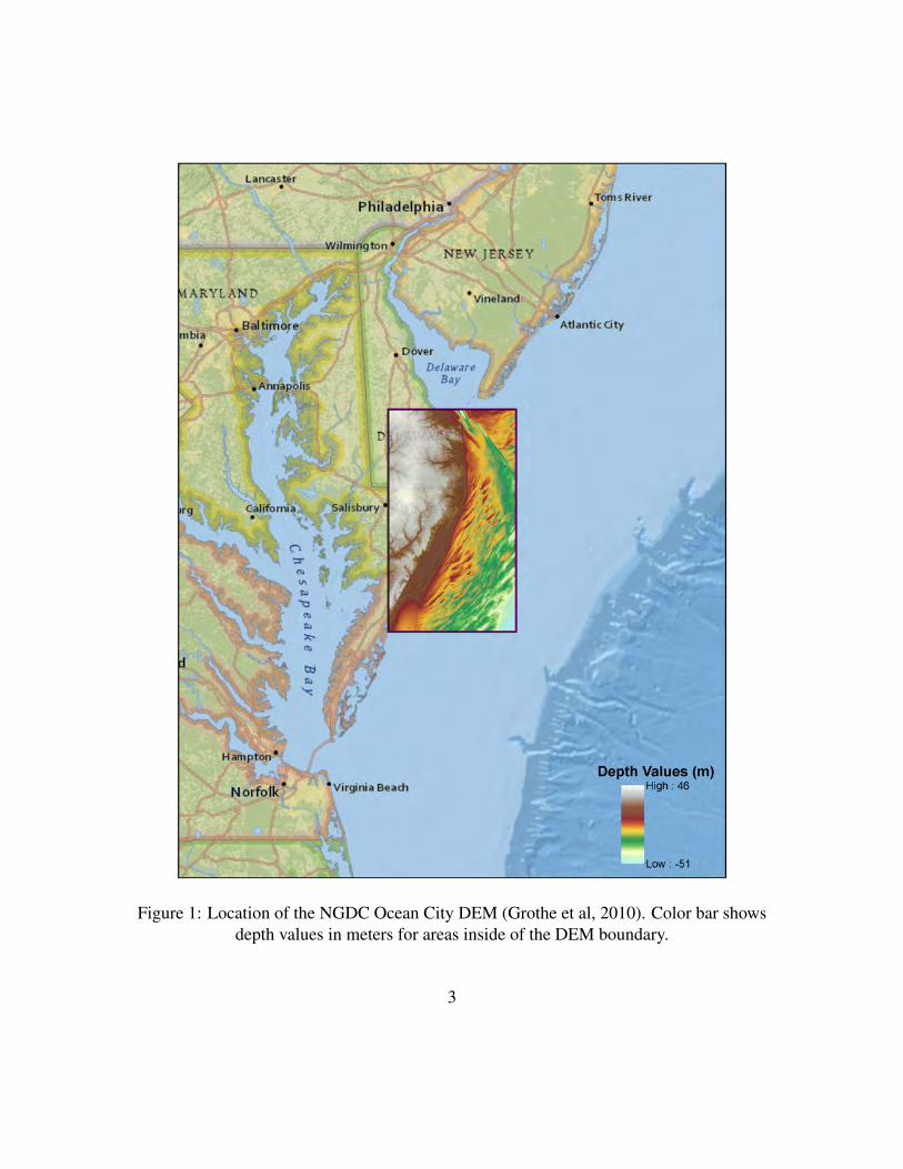
Figure 1: Location of the NGDC Ocean City DEM (Grothe et al, 2010). Color bar showsdepth values in meters for areas inside of the DEM boundary.
3
2.2.1 Coseismic sources
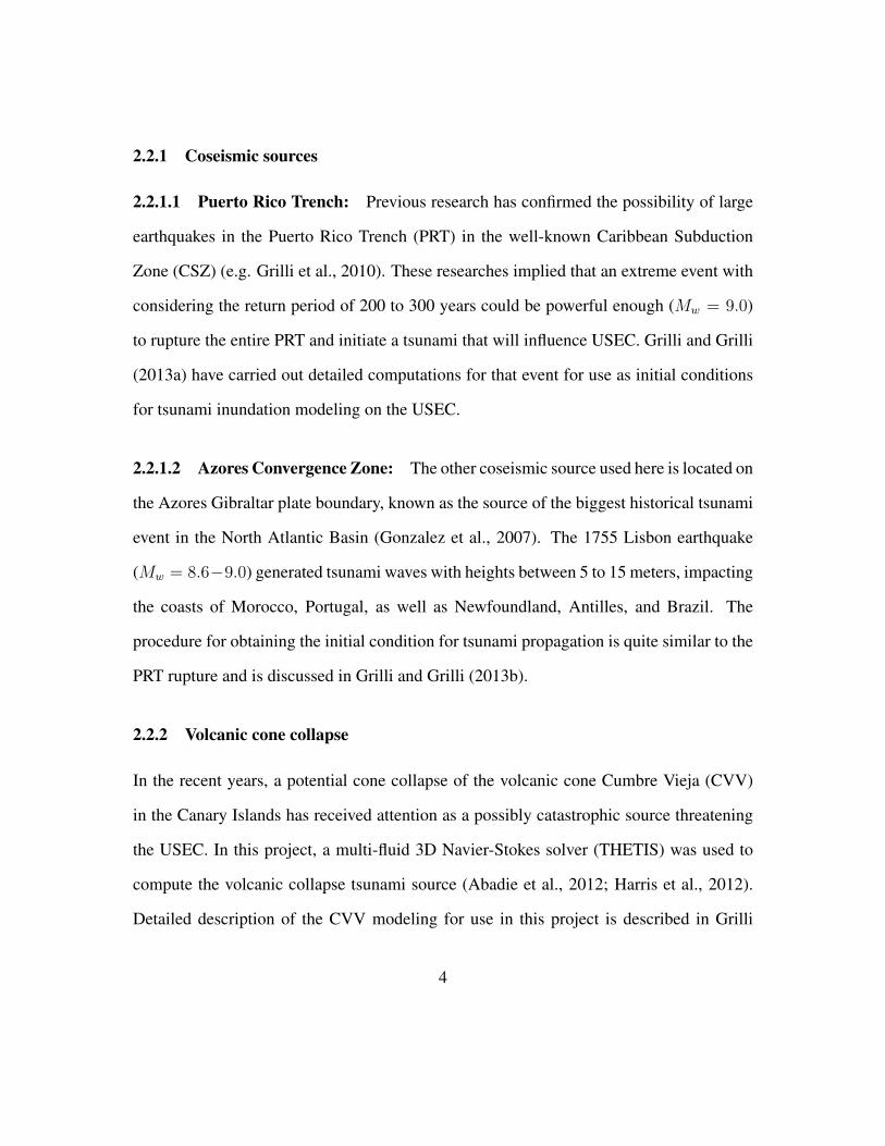
2.2.1.1 Puerto Rico Trench: Previous research has confirmed the possibility of large
earthquakes in the Puerto Rico Trench (PRT) in the well-known Caribbean Subduction
Zone (CSZ) (e.g. Grilli et al., 2010). These researches implied that an extreme event with
considering the return period of 200 to 300 years could be powerful enough (Mw = 9.0)
to rupture the entire PRT and initiate a tsunami that will influence USEC. Grilli and Grilli
(2013a) have carried out detailed computations for that event for use as initial conditions
for tsunami inundation modeling on the USEC.
2.2.1.2 Azores Convergence Zone: The other coseismic source used here is located on
the Azores Gibraltar plate boundary, known as the source of the biggest historical tsunami
event in the North Atlantic Basin (Gonzalez et al., 2007). The 1755 Lisbon earthquake
(Mw = 8.6−9.0) generated tsunami waves with heights between 5 to 15 meters, impacting
the coasts of Morocco, Portugal, as well as Newfoundland, Antilles, and Brazil. The
procedure for obtaining the initial condition for tsunami propagation is quite similar to the
PRT rupture and is discussed in Grilli and Grilli (2013b).
2.2.2 Volcanic cone collapse
In the recent years, a potential cone collapse of the volcanic cone Cumbre Vieja (CVV)
in the Canary Islands has received attention as a possibly catastrophic source threatening
the USEC. In this project, a multi-fluid 3D Navier-Stokes solver (THETIS) was used to
compute the volcanic collapse tsunami source (Abadie et al., 2012; Harris et al., 2012).
Detailed description of the CVV modeling for use in this project is described in Grilli
4
and Grilli (2013c). Two different slide magnitudes were studied for this work; an 80 km3
slide, representing a plausible event in a return period window on the order of 10,000
years, and a 450 km3 source, consistent with estimates of the maximum event for the
geological feature. The magnitude of latter event is significantly larger than all of the
other cases studied in this project. Thus, it was decided to exclude the 450 km3 source
from inundation line calculations, and illustrate its results separately as a representative of
the worst case scenario condition. This is due to the fact that this source return period is
expected to be much more than 10,000 years.
2.2.3 Submarine mass failure
The US East Coast is fronted by a wide continental shelf, which contributes to the dissi-
pation of far-field tsunami sources, and diminishes the damage caused by simulated waves
from these sources on the coastline. On the other hand, it has been noted in literature (e.g.
Grilli et al. 2014) that there is a potential of a Submarine Mass Failure (SMF) on or near
the continental shelf break, causing tsunamis that affect the adjacent coastal areas. Con-
sidering the fact that the only tsunami event that caused fatalities on the US East Coast was
an SMF tsunami (Grand Banks, 1929), it is necessary to study possible impacts and con-
sequences of such catastrophes with respect to heavily populated coastal communities on
the USEC. In this project, four different locations are chosen as the most probable to expe-
rience a submarine mass failure tsunami. The process of obtaining the initial condition for
near-shore propagation and inundation modeling for all of these sources are comprehen-
sively documented in Grilli et al. (2013). The landslide movement is simulated with the
NHWAVE model (Ma et al., 2012; Tehranirad et al., 2012) and the results shown here are
5
interpolated into 500 meter grids for propagation and inundation modeling 800 seconds
after slump movement is initiated (Grilli et al., 2013).
3 Modeling Inputs
3.1 Numerical model
Tsunami propagation and inundation in this study is simulated using the fully nonlinear
Boussinesq model FUNWAVE-TVD (Shi et al, 2012a). FUNWAVE-TVD is a public do-
main open-source code that has been used for modeling tsunami propagation in ocean
basins, nearshore tsunami propagation and inland inundation problems. The code solves
the Boussinesq equations of Chen (2006) in Cartesian coordinates, or of Kirby et al. (2013)
in spherical coordinates. A users manual for each version is provided by Shi et al (2011).
FUNWAVE-TVD has been successfully validated for modeling tsunami wave characteris-
tics such as shoaling, breaking and runup by Tehranirad et al. (2011) following NTHMP
requirements (see Appendix C). Additional description of modeling specifications and in-
put files is provided in Appendix B.
One key specification in the model is the choice of friction coefficient defined for
tsunami simulation. Geist et al. (2009) have performed a study on sensitivity of tsunami
elevation with respect to a range of bottom friction coefficients and demonstrated that
large coefficients will unrealistically damp tsunami wave height. A review of the existing
literature suggests that a value of Cd = 0.0025 represents a reasonable friction coefficient
for tsunami simulations, as suggested by several researchers (e.g. Grilli et al., 2013), and
this value is used here.
6
3.2 Bathymetric Input Data
3.2.1 Ocean City NGDC DEM
In this project, the integrated bathymetric-topographic digital elevation model (DEM) that
is generated by National Geophysical Data Center (NGDC) is used for high-resolution in-
undation mapping for the area around Ocean City, MD (Grothe et al., 2010). This DEM
covers most of the Delmarva Peninsula from the southern part of Delaware Bay down to
Metompkin Bay in Virginia (Figure 1). The horizontal datum is set to be World Geode-
tic System of 1984 (WGS 84), and the vertical datum is mean high water (MHW). The
resolution of Ocean City DEM is 1/3 arc-second, which with respect to study location
means that the North-South resolution is 10.27 meters, and East-West direction grids are
8.10 meters (computed using the latitude in the middle of the domain). All of the runs
in this domain have been performed in Cartesian coordinates. Considering the coverage
area of this grid, the difference between Cartesian grid and spherical grid (Simply com-
paring the total length of domain in Cartesian grid and spherical grid) is about 1.5 meters
for the whole domain. This means that the average offset for each point is of O(10−6)
meters. Therefore, because of the negligible differences between Cartesian and spherical
grids, this grid was used as Cartesian grid directly to capture fully nonlinear effects of the
tsunamis nearshore. Further information about this grid is also given in Table 1.
In the USA the period to determine MHW spans 19 years and is referred to as the Na-
tional Tidal Datum Epoch. For this project, inundation mapping processes have been per-
formed with MHW datum maps following NTHMP requirements (see Appendix C). There
are different approaches to relate MHW to NAVD88 values in the literature, and also, one
7
can use existing datum conversion models to investigate the difference (e.g. Vdatum gen-
erated by NOAA). However, it should be noted that the difference between these values is
not constant for the whole domain. For Ocean City, MD, MHW is at NAVD88+26.3 cm.
For Lewes, DE, MHW is at NAVD+79.25.
3.2.2 NGDC Coastal Relief Model (CRM)
Bathymetry data for shelf regions lying outside the NGDC Ocean City DEM is obtained
from the INGDC’s 3 arc-second U.S. Coastal Relief Model (CRM) (NOAA National Geo-
physical Data Center, U.S. Coastal Relief Model). This data delivers a complete view of
the U.S. coastal areas, combining offshore bathymetry with land topography into a unified
representation of the coast. However, the deeper part of the Ocean beyond the shelf break
is not covered in this data.
3.2.3 ETOPO 1
Bathymetry data for deeper parts of the ocean beyond the shelf break is taken from the
ETOPO1 DEM (Amante and Eakins, 2009). ETOPO1 is a 1 arc-minute global relief
model of Earth’s surface that combines land topography and ocean bathymetry. It was
built from numerous global and regional data sets, and is available in ”Ice Surface” (top of
Antarctic and Greenland ice sheets) and ”Bedrock” (base of the ice sheets) versions. Here,
we use the Bedrock version in areas where the CRM data is not available.
8
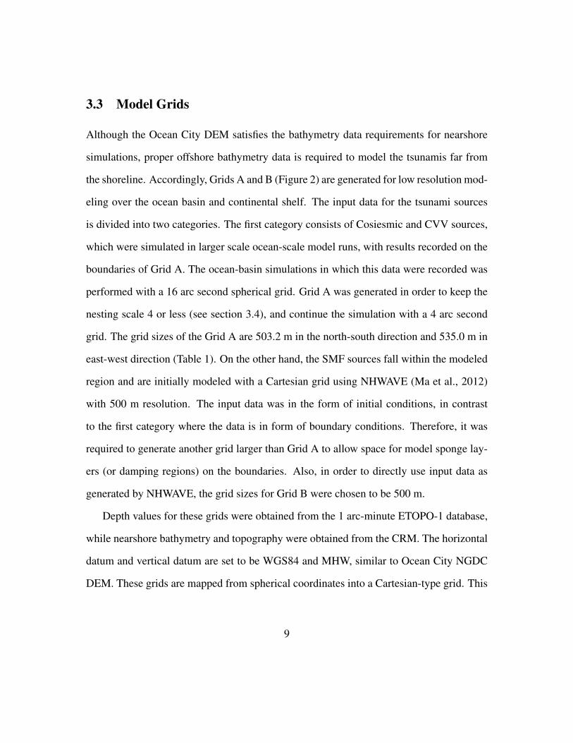
3.3 Model Grids
Although the Ocean City DEM satisfies the bathymetry data requirements for nearshore
simulations, proper offshore bathymetry data is required to model the tsunamis far from
the shoreline. Accordingly, Grids A and B (Figure 2) are generated for low resolution mod-
eling over the ocean basin and continental shelf. The input data for the tsunami sources
is divided into two categories. The first category consists of Cosiesmic and CVV sources,
which were simulated in larger scale ocean-scale model runs, with results recorded on the
boundaries of Grid A. The ocean-basin simulations in which this data were recorded was
performed with a 16 arc second spherical grid. Grid A was generated in order to keep the
nesting scale 4 or less (see section 3.4), and continue the simulation with a 4 arc second
grid. The grid sizes of the Grid A are 503.2 m in the north-south direction and 535.0 m in
east-west direction (Table 1). On the other hand, the SMF sources fall within the modeled
region and are initially modeled with a Cartesian grid using NHWAVE (Ma et al., 2012)
with 500 m resolution. The input data was in the form of initial conditions, in contrast
to the first category where the data is in form of boundary conditions. Therefore, it was
required to generate another grid larger than Grid A to allow space for model sponge lay-
ers (or damping regions) on the boundaries. Also, in order to directly use input data as
generated by NHWAVE, the grid sizes for Grid B were chosen to be 500 m.
Depth values for these grids were obtained from the 1 arc-minute ETOPO-1 database,
while nearshore bathymetry and topography were obtained from the CRM. The horizontal
datum and vertical datum are set to be WGS84 and MHW, similar to Ocean City NGDC
DEM. These grids are mapped from spherical coordinates into a Cartesian-type grid. This
9
means that there are some mapping errors considering the magnitude of these grids. For
example, for the Grid A the total difference between two different coordinate systems is
132 m comparing the arc length (spherical) with the straight line (Cartesian). The average
offset difference for each grid point between two coordinates is 12 cm, which is negligible
considering a grid size of about 500 m. To minimize the error around the mapping area,
the grid is lined up close to the Ocean City DEM. Moreover, the total difference between
spherical and Cartesian coordinates for Grid B is 465 meters. The average offset difference
between two coordinates is 31 cm for each point of this gird. To make the error as small
as possible for the western part of the domain (close to Ocean City, MD), this grid is also
lined up with the mapping area. Therefore, larger error values shows up in the eastern and
southern parts of the domain, which is not of concern because they fall within the sponge
layer region.
Figure 2 shows the location of these grids, as well as the location of the SMF sources
simulated in this project. Further information about these grids are provided in Table 1.
Figure 3 shows the initial surface elevation of each SMF source mapped onto Grid B. The
results of the simulations using Grids A and B were recorded on the Ocean City DEM
boundaries in order to perform higher resolution modeling in nearshore regions. This
process is described in the next section of this document.
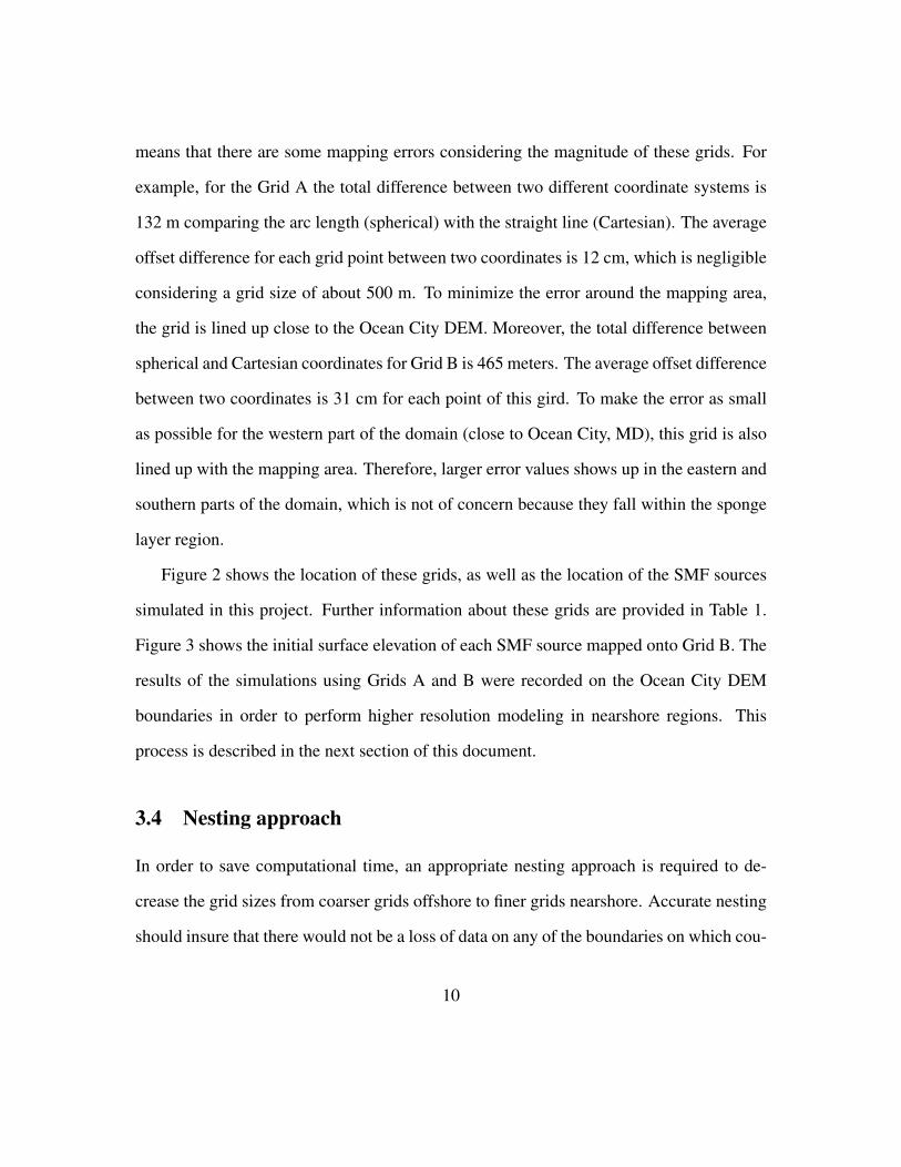
3.4 Nesting approach
In order to save computational time, an appropriate nesting approach is required to de-
crease the grid sizes from coarser grids offshore to finer grids nearshore. Accurate nesting
should insure that there would not be a loss of data on any of the boundaries on which cou-
10
−77 −76 −75 −74 −73 −72 −71 −70 −69 −68 −67
35
36
37
38
39
40
41
42
Longitude(o)
Latitu
de(o
)
Ocean City DEM
Grid A
Grid B
SMF Locations
Figure 2: Locations of the Grids used in this project and also the center of SMF sourcessimulated here.
11
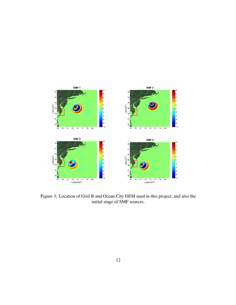
Figure 3: Location of Grid B and Ocean City DEM used in this project, and also theinitial stage of SMF sources.
12
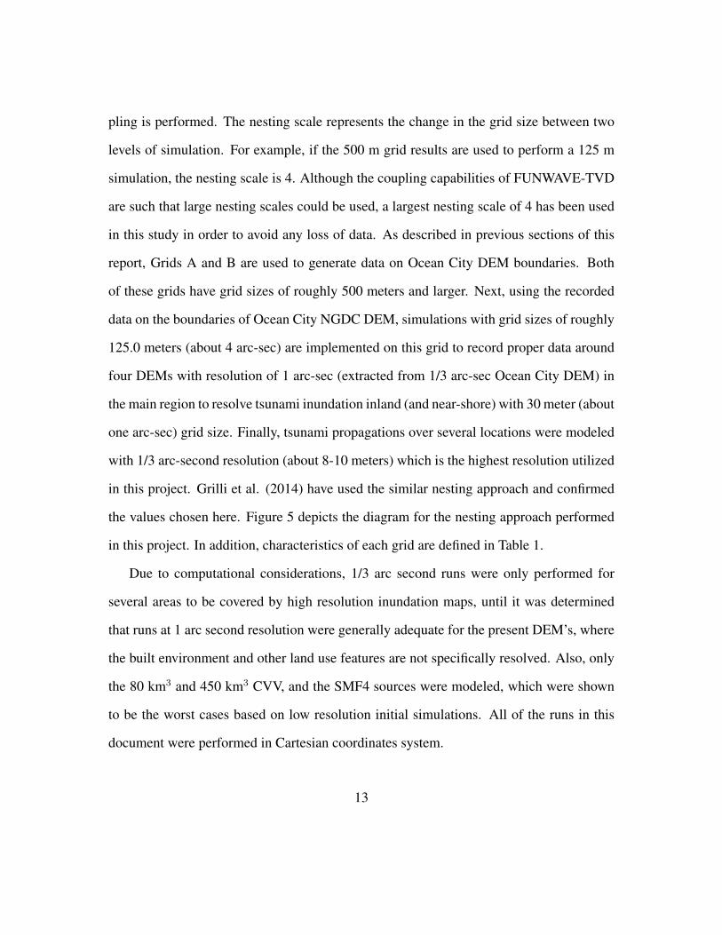
pling is performed. The nesting scale represents the change in the grid size between two
levels of simulation. For example, if the 500 m grid results are used to perform a 125 m
simulation, the nesting scale is 4. Although the coupling capabilities of FUNWAVE-TVD
are such that large nesting scales could be used, a largest nesting scale of 4 has been used
in this study in order to avoid any loss of data. As described in previous sections of this
report, Grids A and B are used to generate data on Ocean City DEM boundaries. Both
of these grids have grid sizes of roughly 500 meters and larger. Next, using the recorded
data on the boundaries of Ocean City NGDC DEM, simulations with grid sizes of roughly
125.0 meters (about 4 arc-sec) are implemented on this grid to record proper data around
four DEMs with resolution of 1 arc-sec (extracted from 1/3 arc-sec Ocean City DEM) in
the main region to resolve tsunami inundation inland (and near-shore) with 30 meter (about
one arc-sec) grid size. Finally, tsunami propagations over several locations were modeled
with 1/3 arc-second resolution (about 8-10 meters) which is the highest resolution utilized
in this project. Grilli et al. (2014) have used the similar nesting approach and confirmed
the values chosen here. Figure 5 depicts the diagram for the nesting approach performed
in this project. In addition, characteristics of each grid are defined in Table 1.
Due to computational considerations, 1/3 arc second runs were only performed for
several areas to be covered by high resolution inundation maps, until it was determined
that runs at 1 arc second resolution were generally adequate for the present DEM’s, where
the built environment and other land use features are not specifically resolved. Also, only
the 80 km3 and 450 km3 CVV, and the SMF4 sources were modeled, which were shown
to be the worst cases based on low resolution initial simulations. All of the runs in this
document were performed in Cartesian coordinates system.
13

6 6.5 7 7.5 8 8.5 9 9.5 10−10
−5
0
5
Elev
atio
n(m
) CVV Source (450 km3 slide)
6 6.5 7 7.5 8 8.5 9 9.5 10−2
0
2CVV Source (80 km3 slide)
Elev
atio
n(m
)
6 6.5 7 7.5 8 8.5 9 9.5 10−0.5
0
0.5
Elev
atio
n(m
) Lisbon Source
2 2.5 3 3.5 4 4.5 5 5.5 6−1
0
1
2
Elev
atio
n(m
)
Time (Hours)
Puerto Rico Source
Figure 4: Gauge data at the southeastern edge of Grid A for coseismic and volcaniccollapse sources
14
Gri
dN
umbe
rsG
rid
Size
(m)
Bou
ndar
yC
oord
inat
esG
rid
Nam
emx
ny
dx
dy
EW
SN
Gri
dA
1100
900
503.
2053
5.50
-69.
25-7
5.70
37.4
541
.80
Gri
dB
1500
1500
500.
0050
0.00
-67.
50-7
6.00
35.0
042
.00
OC
4arc
(Sam
ebo
ndar
ies
with
Oce
anC
ityD
EM
)62
710
7297
.20
123.
24-7
4.71
-75.
5837
.68
38.8
7O
C1a
rc1
1000
1000
24.3
030
.81
-75.
02-7
5.30
38.5
438
.83
OC
1arc
210
0012
0024
.30
30.8
1-7
5.02
-75.
3038
.24
38.5
7O
C1a
rc3
1200
1000
24.3
030
.81
-75.
12-7
5.45
37.9
838
.26
OC
1arc
412
0010
0024
.30
30.8
1-7
5.22
-75.
5637
.73
38.0
1L
ewes
and
Reh
obot
hB
each
(1/3
arc-
sec)
(OC
10m
1)67
512
008.
1010
.27
-75.
06-7
5.12
38.7
038
.81
Dew
ey(1
/3ar
c-se
c)(O
C10
m2)
900
900
8.10
10.2
7-7
5.05
-75.
1438
.62
38.7
1B
etha
nyB
each
(1/3
arc-
sec)
(OC
10m
3)90
090
08.
1010
.27
-75.
04-7
5.12
38.4
838
.57
Oce
anC
ity1
(1/3
arc-
sec)
(OC
10m
4)54
015
008.
1010
.27
-75.
04-7
5.09
38.3
538
.50
Oce
anC
ity2
(1/3
arc-
sec)
(OC
10m
5)90
090
08.
1010
.27
-75.
06-7
5.14
38.2
938
.37
Chi
ncot
eagu
e(1
/3ar
c-se
c)(O
C10
m6)
900
1200
8.10
10.2
7-7
5.31
-75.
4037
.85
37.9
6
Tabl
e1:
Gri
dsp
ecifi
catio
nfo
rall
ofth
egr
ids
used
inth
ispr
ojec
t
15
−76 −75 −74 −73 −72 −71 −70 −69 −6836
37
38
39
40
41
42
Longitude(o)
Latit
ude(
o )
Ocean City DEMN. US reg.
−76 −75 −74 −73 −72 −71 −70 −69 −68 −67
35
36
37
38
39
40
41
42
Longitude(o)
Latit
ude(
o )
Ocean City DEMGrid AGrid BSMF Locations
Service Layer Credits: Copyright:© 2013 Esri,DeLorme, NAVTEQ, TomTomSource: Esri, DigitalGlobe, GeoEye, i-cubed,USDA, USGS, AEX, Getmapping, Aerogrid,IGN, IGP, swisstopo, and the GIS User
75°0'0"W75°20'0"W
38°40'0"N
38°20'0"N
38°0'0"N
37°40'0"N
1/3 Arc-Sec
1 Arc-Sec
4 Arc-Sec
Service Layer Credits: Copyright:© 2013 Esri,DeLorme, NAVTEQ, TomTomSource: Esri, DigitalGlobe, GeoEye, i-cubed,USDA, USGS, AEX, Getmapping, Aerogrid,IGN, IGP, swisstopo, and the GIS User
75°0'0"W75°5'0"W75°10'0"W
38°50'0"N
38°40'0"N
38°30'0"N
38°20'0"N
Longitude (o)
Longitude (o)
Latitude ( o)
Latit
ude
(o)
Figure 5: This figure demonstrates the nesting approach diagram. The figure on the topleft depicts the Grid A and B as well as the location of the Ocean City DEM. The figureon the right show the 1 arc-sec grids described in Table 1. Also, in the bottom left figure
the 1/3 arc-sec domains are shown (Also described in Table 1).
16
4 Results
This section describes the data recorded for each inundation simulation and its organiza-
tion as ArcGIS rasters for subsequent map development. The tsunami arrival time is an
essential piece of information for evacuation planners. The results are categorized into
onshore and offshore results. The onshore results depict the characteristics of the tsunami
on the land during inundation. Onshore tsunami effects are mainly demonstrated through
three parameters,
1. Maximum inundation depth
2. Maximum velocity
3. Maximum momentum flux
Yeh (2007) reported different forces created by a tsunami on structures and concluded hav-
ing the three mentioned quantities, one can calculate all of the possible forces on onshore
structures associated with tsunamis. Moreover, tsunamis can affect ship navigation; there-
fore, in order to cover maritime planning and navigational issues during a tsunami, three
other parameters are recorded and depicted offshore in this project. These three offshore
parameters include,
1. Maximum vorticity
2. Maximum velocity
3. Maximum recorded water surface elevation
17

All six variables are recorded for each of the modeling domains introduced in Table 1 for
all of the tsunami sources discussed in previous sections. Appropriate rasters are generated
which are compatible with ArcGIS and other GIS software for mapping purposes. Finally,
the inundation line, which is calculated from the envelope of tsunami inundation extent
for each source, will be presented.
4.1 Arrival time
Tsunami arrival time plays an important role in evacuation planning during the occurrence
of an event. Regional warning centers use seismic data of the recent earthquakes to de-
termine the possibility of a tsunami threat. Some of those systems are capable of issuing
tsunami warning within 5 minutes. Therefore, as a result of tsunami propagation simu-
lation, it is vital to report the arrival time of each tsunami. Here, the arrival time of the
tsunami is based on the time that the first tsunami bore passes the shoreline. Table 2 re-
ports tsunami arrival times for several places located in Ocean City NGDC DEM. For each
location, arrival times of all different tsunami sources have been reported. The arrival time
for each city in Table 2 is a value for that particular location (for example, averaged along
Ocean City, MD shoreline) with about a 5 minute error margin. Since tsunami propagation
in the ocean is constrained by bathymetry, the propagation of tsunamis toward the Ocean
City area is quite similar for all of the different sources. The southern part of the domain
(e.g. Ocean City, MD) is the first spot that would face the tsunami. However, within 10 to
15 minutes difference, the northern part of the domain that is facing Atlantic Ocean (e.g.
Rehoboth Beach) will be affected by the tsunami as well. Finally, within 30 to 40 minutes
lag in comparison with the southern parts of the domain, tsunami would reach parts of the
18
40 60 80 100 120 140−2
0
2SMF1
40 60 80 100 120 140−2
0
2SMF2
40 60 80 100 120 140−2
0
2SMF3
40 60 80 100 120 140−5
0
5SMF4
240 260 280 300 320 340 360−2
0
2PR
500 520 540 560 580 600 620−0.5
0
0.5LIS
480 500 520 540 560 580 600−5
0
5CVV
Service Layer Credits: Copyright:© 2013 Esri,DeLorme, NAVTEQ, TomTomSource: Esri, DigitalGlobe, GeoEye, i-cubed,USDA, USGS, AEX, Getmapping, Aerogrid,IGN, IGP, swisstopo, and the GIS User
75°0'0"W
75°0'0"W
75°4'0"W
75°4'0"W
75°8'0"W
75°8'0"W
38°45'0"N
38°40'0"N
38°35'0"N
38°30'0"N
38°25'0"N
38°20'0"N
Time After Tsunami Initiation (min)
Sur
face
Ele
vatio
n (m
)
Figure 6: Recorded Surface Elevation for NOAA Gauges which are located in OceanCity DEM, Ocean City (Green), Cape Henlopen (Red), and Lewes (Blue)
19
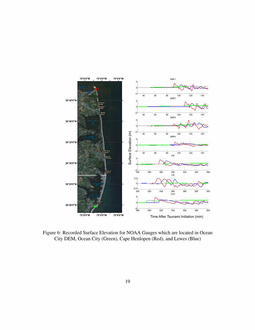
domain inside Delaware Bay (e.g. Lewes). Figure 6 demonstrates the location of NOAA
gauges and their recorded surface elevation for all of the sources. The tsunami impact
differences between the areas behind the barriers and areas facing the ocean directly is
clear in the figure. The Cape Henlopen, DE gauge that is located in the ocean experience
much stronger signal in comparison to Ocean City, MD, where the guage is located behind
the barrier. Basically the protected areas behind barrier islands experience tsunami effects
more like a storm surge but with a much smaller time scale. Also, the Lewes, DE gauge
data is similar to Cape Henlopen with about 10 to 15 minutes lag. SMF sources are clearly
the closest source to the location of study, and will reach the entire domain within 1 to
2 hours. The tsunami induced by Puerto Rico Trench (PRT) will affect the Ocean City
greater area between 4 to 5 hours after the earthquake. The Lisbon historic event and the
Cumbre Vieja Volcanic collapse (CVV) sources have similar transoceanic travel time, and
will influence the domain 8 to 9 hours after the incident.
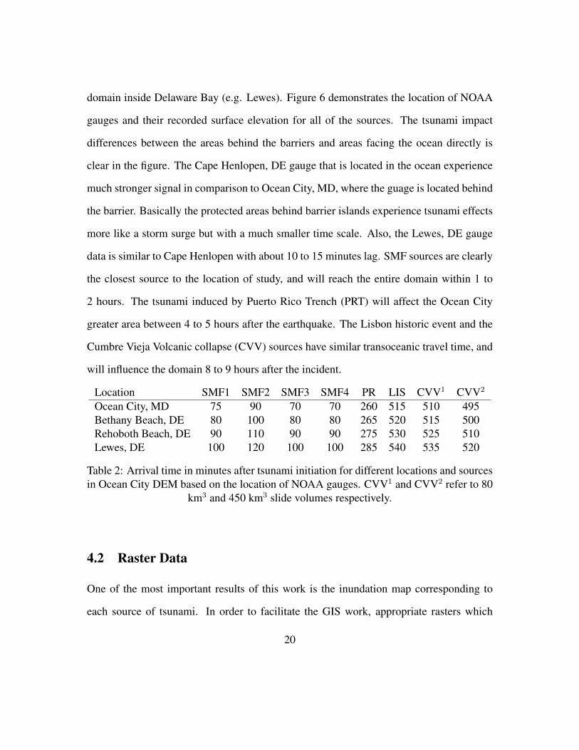
Location SMF1 SMF2 SMF3 SMF4 PR LIS CVV1 CVV2
Ocean City, MD 75 90 70 70 260 515 510 495Bethany Beach, DE 80 100 80 80 265 520 515 500Rehoboth Beach, DE 90 110 90 90 275 530 525 510Lewes, DE 100 120 100 100 285 540 535 520
Table 2: Arrival time in minutes after tsunami initiation for different locations and sourcesin Ocean City DEM based on the location of NOAA gauges. CVV1 and CVV2 refer to 80
km3 and 450 km3 slide volumes respectively.
4.2 Raster Data
One of the most important results of this work is the inundation map corresponding to
each source of tsunami. In order to facilitate the GIS work, appropriate rasters which
20
are compatible with any GIS software such as ArcGIS are created for all of the grids
mentioned in Table 1. As an example, Figure 7 depicts the inundation depth for SMF4
for the Ocean City DEM grid with 4 arc-second resolution. In this figure the domains in
which 1 Arc-second resolution runs have been performed are displayed as well.
Figures 8-11 show the maximum inundation depth for the 1 Arc-second domains
shown in Figure 7. These figures provide a comparison for different sources studied in
this project. This includes the envelope inundation map for SMF and coseismic sources
as well as both CVV sources. The inundation depth for SMF sources are similar to each
other, however, the inundation depth values for SMF4 is larger for the most part in com-
parison to the other SMF sources. This is probably because of the fact that the SMF4 is the
closest SMF source to the location of study. Also, the Puerto Rico event is the dominant
cosiesmic source by far, and its inundation pattern is similar to SMF sources with some dif-
ferences especially behind the barriers. Since coseismic sources have larger wavelengths,
they are able to penetrate behind the barriers with less attenuation in comparison to SMF
sources. Figures 8-11 show that the CVV 450 km3 source is clearly the dominant source
for the area studied here, and represents worst case scenario by far in comparison to other
sources. However, because its return period is estimated to be beyond 10000 years, it is
excluded from inundation line calculations at this point. The 80 km3 slide CVV has a sim-
ilar inundation pattern to Puerto Rico source and SMF4. Except for some few locations it
is the dominant source among all other sources, excluding the CVV 450 km3 slide source.
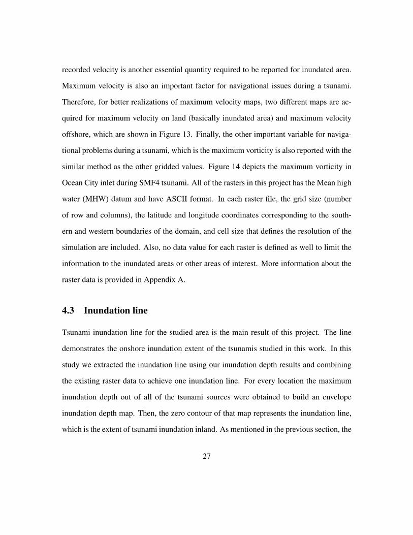
The other important criteria required to be reported for inundated area, is the maxi-
mum momentum flux. Figure 12 is an example of the maximum momentum flux which
is extracted from Bethany Beach 1/3 Arc-sec domain for the SMF4 tsunami. Maximum-
21
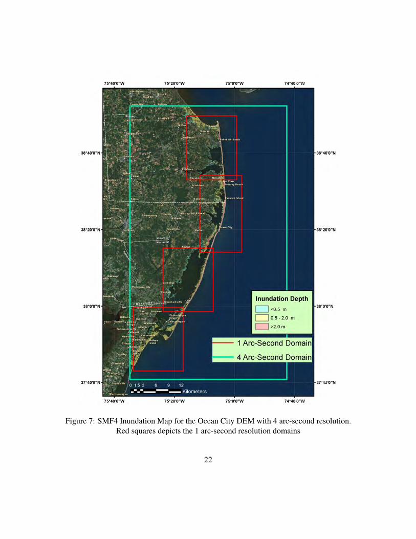
Figure 7: SMF4 Inundation Map for the Ocean City DEM with 4 arc-second resolution.Red squares depicts the 1 arc-second resolution domains
22
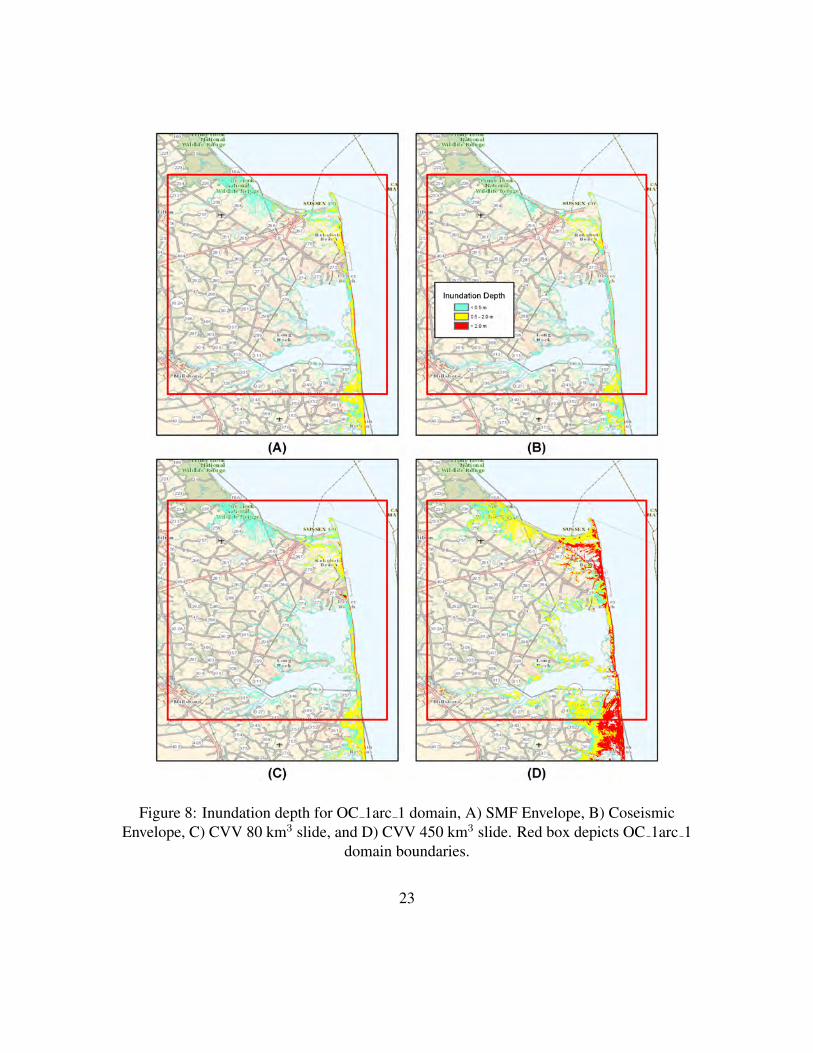
Figure 8: Inundation depth for OC 1arc 1 domain, A) SMF Envelope, B) CoseismicEnvelope, C) CVV 80 km3 slide, and D) CVV 450 km3 slide. Red box depicts OC 1arc 1
domain boundaries.
23
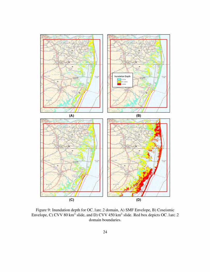
Figure 9: Inundation depth for OC 1arc 2 domain, A) SMF Envelope, B) CoseismicEnvelope, C) CVV 80 km3 slide, and D) CVV 450 km3 slide. Red box depicts OC 1arc 2
domain boundaries.
24
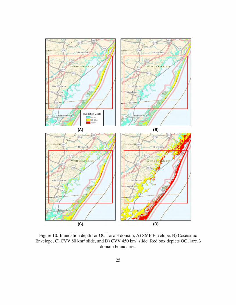
Figure 10: Inundation depth for OC 1arc 3 domain, A) SMF Envelope, B) CoseismicEnvelope, C) CVV 80 km3 slide, and D) CVV 450 km3 slide. Red box depicts OC 1arc 3
domain boundaries.
25
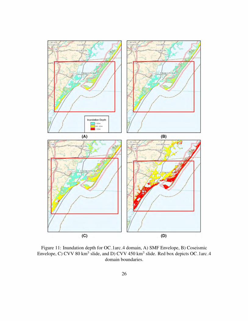
Figure 11: Inundation depth for OC 1arc 4 domain, A) SMF Envelope, B) CoseismicEnvelope, C) CVV 80 km3 slide, and D) CVV 450 km3 slide. Red box depicts OC 1arc 4
domain boundaries.
26
recorded velocity is another essential quantity required to be reported for inundated area.
Maximum velocity is also an important factor for navigational issues during a tsunami.
Therefore, for better realizations of maximum velocity maps, two different maps are ac-
quired for maximum velocity on land (basically inundated area) and maximum velocity
offshore, which are shown in Figure 13. Finally, the other important variable for naviga-
tional problems during a tsunami, which is the maximum vorticity is also reported with the
similar method as the other gridded values. Figure 14 depicts the maximum vorticity in
Ocean City inlet during SMF4 tsunami. All of the rasters in this project has the Mean high
water (MHW) datum and have ASCII format. In each raster file, the grid size (number
of row and columns), the latitude and longitude coordinates corresponding to the south-
ern and western boundaries of the domain, and cell size that defines the resolution of the
simulation are included. Also, no data value for each raster is defined as well to limit the
information to the inundated areas or other areas of interest. More information about the
raster data is provided in Appendix A.
4.3 Inundation line
Tsunami inundation line for the studied area is the main result of this project. The line
demonstrates the onshore inundation extent of the tsunamis studied in this work. In this
study we extracted the inundation line using our inundation depth results and combining
the existing raster data to achieve one inundation line. For every location the maximum
inundation depth out of all of the tsunami sources were obtained to build an envelope
inundation depth map. Then, the zero contour of that map represents the inundation line,
which is the extent of tsunami inundation inland. As mentioned in the previous section, the
27
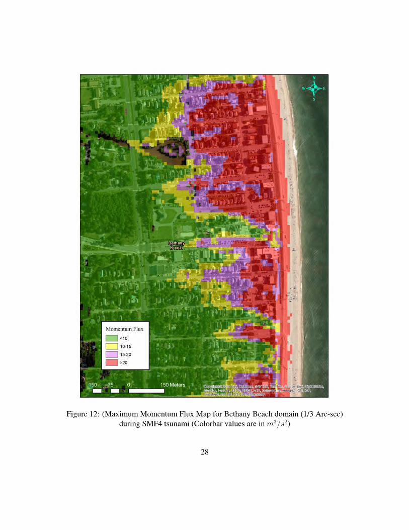
Figure 12: (Maximum Momentum Flux Map for Bethany Beach domain (1/3 Arc-sec)during SMF4 tsunami (Colorbar values are in m3/s2)
28
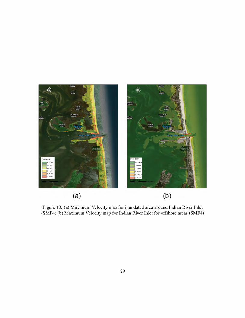
Figure 13: (a) Maximum Velocity map for inundated area around Indian River Inlet(SMF4) (b) Maximum Velocity map for Indian River Inlet for offshore areas (SMF4)
29
Figure 14: Maximum Vorticity map for the area around Ocean City inlet
30
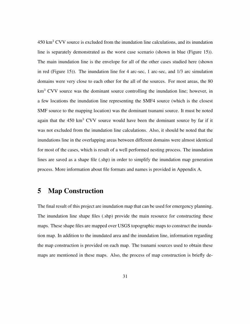
450 km3 CVV source is excluded from the inundation line calculations, and its inundation
line is separately demonstrated as the worst case scenario (shown in blue (Figure 15)).
The main inundation line is the envelope for all of the other cases studied here (shown
in red (Figure 15)). The inundation line for 4 arc-sec, 1 arc-sec, and 1/3 arc simulation
domains were very close to each other for the all of the sources. For most areas, the 80
km3 CVV source was the dominant source controlling the inundation line; however, in
a few locations the inundation line representing the SMF4 source (which is the closest
SMF source to the mapping location) was the dominant tsunami source. It must be noted
again that the 450 km3 CVV source would have been the dominant source by far if it
was not excluded from the inundation line calculations. Also, it should be noted that the
inundations line in the overlapping areas between different domains were almost identical
for most of the cases, which is result of a well performed nesting process. The inundation
lines are saved as a shape file (.shp) in order to simplify the inundation map generation
process. More information about file formats and names is provided in Appendix A.
5 Map Construction
The final result of this project are inundation map that can be used for emergency planning.
The inundation line shape files (.shp) provide the main resource for constructing these
maps. These shape files are mapped over USGS topographic maps to construct the inunda-
tion map. In addition to the inundated area and the inundation line, information regarding
the map construction is provided on each map. The tsunami sources used to obtain these
maps are mentioned in these maps. Also, the process of map construction is briefly de-
31
Figure 15: Tsunami inundation Line for Ocean City NGDC DEM area based on tsunamisources simulated in this project. The blue boxes show the location of the inundation
maps discussed in Section 5.
32
scribed on the map. Figures 16-19 show the draft inundation maps for the “Lewes, DE, and
Rehoboth Beach, DE”, “Bethany Beach, DE, “Ocean City, MD” communities in 1:30,000
scale, as well as an inundation map for“Chincoteague, VA” in 1:40,000 scale. The location
of these maps are shown in Figure 15. The basemap for these figures are the USGS topo-
graphic maps obtained from (http://basemap.nationalmap.gov/ArcGIS/rest/services/USGSTopo/MapServer).
33
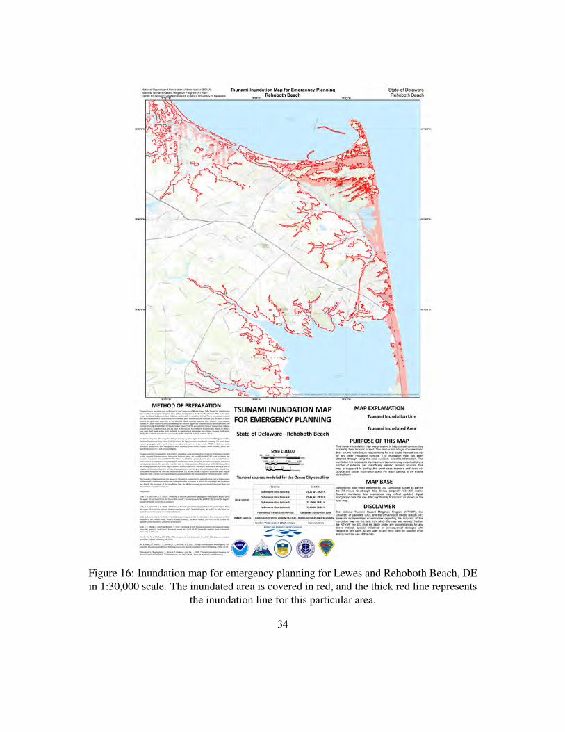
Figure 16: Inundation map for emergency planning for Lewes and Rehoboth Beach, DEin 1:30,000 scale. The inundated area is covered in red, and the thick red line represents
the inundation line for this particular area.
34
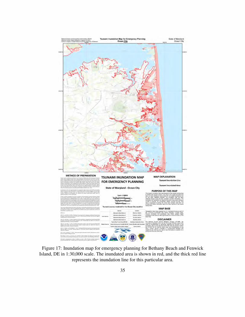
Figure 17: Inundation map for emergency planning for Bethany Beach and FenwickIsland, DE in 1:30,000 scale. The inundated area is shown in red, and the thick red line
represents the inundation line for this particular area.
35
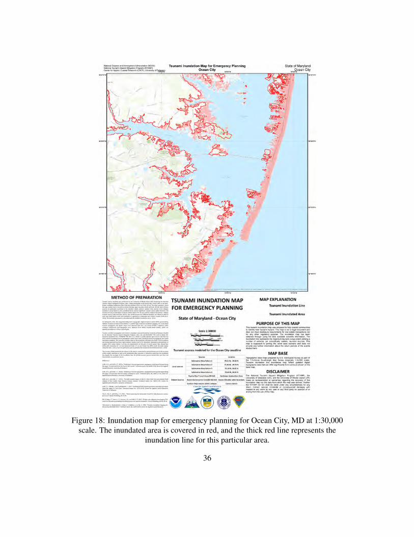
Figure 18: Inundation map for emergency planning for Ocean City, MD at 1:30,000scale. The inundated area is covered in red, and the thick red line represents the
inundation line for this particular area.
36
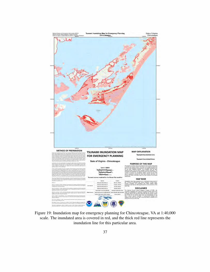
Figure 19: Inundation map for emergency planning for Chincoteague, VA at 1:40,000scale. The inundated area is covered in red, and the thick red line represents the
inundation line for this particular area.
37
References
Amante, C. and Eakins, B.W., 2009, “ETOPO1 1 Arc-Minute Global Relief Model:
Procedures, Data Sources and Analysis”, NOAA Technical Memorandum NESDIS
NGDC-24. National Geophysical Data Center, NOAA. doi:10.7289/V5C8276M.
Abadie, S. M., Harris, J. C., Grilli, S. T., and Fabre, R., 2012, “Numerical modeling of
tsunami waves generated by the flank collapse of the Cumbre Vieja Volcano (La
Palma, Canary Islands) Tsunami source and near field effects”, Journal of Geophys-
ical Research, 117(C5), C05030, doi:10.1029/2011JC007646.
Atlantic and Gulf of Mexico Tsunami Hazard Assessment Group, 2008, “Evaluation of
Tsunami Sources with the Potential to Impact the U.S. Atlantic and Gulf Coasts - A
Report to the Nuclear Regulatory Commission”, U.S. Geological Survey Adminis-
trative Report.
Barkan, R., Ten Brink, U. S., and Lin, J., 2009, “Far field tsunami simulations of the
1755 Lisbon earthquake: Implications for tsunami hazard to the US East Coast and
the Caribbean”, Marine Geology, 264, 109-122.
Chen, Q., 2006, “Fully nonlinear Boussinesq-type equations for waves and currents over
porous beds”, J. Engin. Mech. 132, 220-230.
Divins, D. L., and Metzger, D., 2003, “NGDC coastal relief model. National Geophysical
Data Center”, (http://www. ngdc. noaa. gov/mgg/coastal/coastal. html).
38
Geist, E. L., Lynett, P. J., and Chaytor, J. D., 2009, “Hydrodynamic modeling of tsunamis
from the Currituck landslide”, Marine Geology, 264, 41-52.
Gonzalez, F. I., et al., 2007, “Scientific and technical issues in tsunami hazard assessment
of nuclear power plant sites.” NOAA Tech. Memo. OAR PMEL 136.
Grilli, S. T., O’Reilly, C., Harris, J. C., Tajalli Bakhsh, T., Tehranirad, B., Banihashemi,
S., Kirby, J. T., Baxter, C. D. P., Eggeling, T., Ma, G., and Shi, F., 2014, “Modeling
of SMF tsunami hazard along the upper US East Coast: Detailed impact around
Ocean City, MD”, Natural Hazards, in press.
Grilli, A. R., and Grilli, S. T., 2013a, “Modeling of tsunami generation, propagation and
regional impact along the upper US East Coast from the Puerto Rico trench”, Re-
search Report, No. CACR-13-02, Center for Applied Coastal Research, University
of Delaware. http://chinacat.coastal.udel.edu/nthmp/grilli-grilli-cacr-13-03.pdf
Grilli, A. R., and Grilli, S. T., 2013b, “Modeling of tsunami generation, propagation
and regional impact along the upper US East Coast from the Azores convergence
zone”, Research Report, No. CACR-13-04, Center for Applied Coastal Research,
University of Delaware. http://chinacat.coastal.udel.edu/nthmp/grilli-grilli-cacr-13-
02.pdf
Grilli, A. R., and Grilli, S. T., 2013c, “Far-field tsunami impact on the U.S. East Coast
from and extreme flank collapse of the Cumbre Vieja Volcano (Canary Islands)”,
Research Report, No. CACR-13-03, Center for Applied Coastal Research, Univer-
sity of Delaware. http://chinacat.coastal.udel.edu/nthmp/grilli-grilli-cacr-13-04.pdf
39
Grilli, S. T., O’Reilly, C. and Tajalli Bakhsh, T., 2013, “Modeling of SMF tsunami
generation and regional impact along the upper US East Coast”, Research Report
No. CACR-13-05, Center for Applied Coastal Research, University of Delaware.
http://chinacat.coastal.udel.edu/nthmp/grilli-etal-cacr-13-05.pdf
Grilli, S. T., Dubosq, S., Pophet, N., Perignon, Y., Kirby, J. T., and Shi, F., 2010, “Nu-
merical simulation and first-order hazard analysis of large co-seismic tsunamis gen-
erated in the Puerto Rico trench: near-field impact on the North shore of Puerto
Rico and far-field impact on the US East Coast”, Natural Hazards and Earth System
Sciences, 10, 2109-2125.
Grilli, S. T., Taylor, O. D. S., Baxter, C. D., and Maretzki, S. , 2009, “A probabilistic
approach for determining submarine landslide tsunami hazard along the upper east
coast of the United States”, Marine Geology, 264 (1), 74-97.
Grothe, P. R, Taylor, L. A, Eakins, B. W, Warnken, R. R, Carignan, K. S, Lim, E,
Caldwell, R. J, and Friday, D.Z., 2010, “Digital Elevation Model of Ocean City,
Maryland: Procedures, Data and Analysis”, NOAA Technical Memorandum NES-
DIS NGDC-37, , Dept. of Commerce, Boulder, CO, 37 pp.
Harris, J. C., Tehranirad, B., Grilli, A. R., Grilli, S. T., Abadie, S., Kirby, J. T., Shi, F.,
2014, “Far-field tsunami hazard on the western European and US east coasts from
a large scale flank collapse of the Cumbre Vieja volcano, La Palma”,Submitted to
PAG.
Harris, J. C., Grilli, S. T., Abadie, S., and Tajalli Bakhsh, T. , 2012, “Near-and far-field
tsunami hazard from the potential flank collapse of the Cumbre Vieja Volcano”,
40
In Proceedings of the 22nd Offshore and Polar Engng, Conf.(ISOPE12), Rodos,
Greece, June 17-22, 2012).
Kirby, J. T., Shi, F., Tehranirad, B., Harris, J. C., and Grilli, S. T., 2013, “Dispersive
tsunami waves in the ocean: Model equations and sensitivity to dispersion and Cori-
olis effects”, Ocean Modelling,62, 39-55.
Ma, G., Shi, F., and Kirby, J. T., 2012, “Shock-capturing non-hydrostatic model for fully
dispersive surface wave processes”, Ocean Modelling, 43, 22-35.
NOAA National Geophysical Data Center, U.S. Coastal Relief Model, Retrieved date
goes here, http://www.ngdc.noaa.gov/mgg/coastal/crm.html
Shi, F., Kirby, J. T., Harris, J. C., Geiman, J. D., and Grilli, S. T., 2012a , “A high-order
adaptive time-stepping TVD solver for Boussinesq modeling of breaking waves and
coastal inundation”, Ocean Modelling, 43-44, 36-51.
Shi, F., Kirby, J. T., and Tehranirad, B. , 2012 b, “Tsunami benchmark results for spher-
ical coordinate version of FUNWAVE-TVD (Version 2.0)” , Research Report, No.
CACR 2012-02, Center for Applied Coastal Research Report, University of Delaware,
Newark, Delaware. http://chinacat.coastal.udel.edu/papers/shi-etal-cacr-12-02-version2.0.pdf
Shi, F., Kirby, J. T., Tehranirad, B., Harris, J. C., Grilli, S. T., 2011, “FUNWAVE-TVD
Fully Nonlinear Boussinesq Wave Model with TVD Solver Documentation and
Users Manual”, Research Report, No. CACR-11-04, Center for Applied Coastal Re-
search Report, University of Delaware, Newark, Delaware. http://chinacat.coastal.udel.edu/papers/shi-
etal-cacr-11-04-version2.1.pdf
41
Synolakis, C. E., Bernard, E. N., Titov, V. V., Kanoglu, U. and Gonzalez, F. I., 2008,
“Validation and verification of tsunami numerical models”, Pure and Applied Geo-
physics, 165, 2197-2228.
Tehranirad, B., Shi, F., Kirby, J. T., Harris, J. C., and Grilli, S. T., 2011, “Tsunami bench-
mark results for fully nonlinear Boussinesq wave model FUNWAVE-TVD. Version
1.0”, Research Report, No. CACR-11-02, Center for Applied Coastal Research,
University of Delaware.
Tehranirad, B., J. T. Kirby, G. Ma, and F. Shi, 2012, “Tsunami benchmark results for non-
hydrostatic wave model NHWAVE version 1.1.”, Tech. rep., Research Report, No.
CACR-12-03, Center for Applied Coastal Research Report, University of Delaware,
Newark, Delaware. http://chinacat.coastal.udel.edu/papers/tehranirad-etal-cacr-11-
02-version1.0.pdf
Yeh, H., 2007, “Tsunami load determination for on-shore structures”, In Proc. Fourth
International Conference on Urban Earthquake Engineering, 415-422
Yeh, H. H. J., Robertson, I., and Preuss, J., 2005, “Development of design guidelines for
structures that serve as tsunami vertical evacuation sites (p. 34)”, Washington State
Department of Natural Resources, Division of Geology and Earth Resources.
42
Appendix A Gridded Data Information
In order to facilitate GIS work used to report tsunami inundation simulation results, the
output data is saved in ESRI Arc ASCII grid format, which is compatible with GIS soft-
ware such as ArcGIS. For each file, the grid spacing could have three different values
((dx, dy)= (8.10,10.27) m, (24.30,30.81) m, and (97.20,123.24) m) depending on the do-
main, and the coordinate system is based on Geographic decimal degrees (Longitude and
Latitude). Also, the vertical datum of all rasters is mean high water (MHW), and the hori-
zontal datum is World Geodetic System of 1984 (WGS 84). The name of each file implies
some information about the file contents as well. The first part defines the type of data and
could be one of the following,
Inun . . . Onshore inundation depth
Inun area . . . Depicts the inundated area (inundation line)
Hmax. . . Maximum recorded offshore water surface elevation
Mfmx . . . Maximum recorded onshore momentum flux
Uwet. . . Maximum recorded onshore velocity
Udry. . . Maximum recorded offshore velocity
vorm. . . Maximum recorded offshore vorticity
depth. . . depth
The rasters including inundation depth, maximum momentum flux, and maximum onshore
velocity (udry) are only meaningful onshore (for initially dry points, basically inundated
points), and by using the bathymetry data, nodata values have been defined for onshore
A–1
points in these rasters (nodata value=-9999). The reverse is performed for maximum vor-
ticity and maximum offshore velocity (uwet) rasters by setting the offshore values to -9999
to just consider the initially wet points in the domain. The second part of the raster name
defines the tsunami source used to obtain that data. This could be seven different sources
and are categorized as follows,
SMF1-4. . . Submarine Mass Failure 1-4
PR. . . Puerto Rico Trench
LIS. . . Lisbon Source
CVV. . . Cumbre Vieja Volcanic Collapse.
In each file, the grid sizes (mx,ny), the coordinates for south west corner of the domain,
and the grid size are included in the file heading as well as a nodata value through the
following format,
ncols 9397
nrows 12853
xllcorner -75.580046296295
yllcorner 37.679953703705
cellsize 9.2592589999999e-005
NODATA value -9999
A–2
Beneath the file heading, the corresponding values to each point are written in the file
with the format that starts from the southwest edge of the domain, and writes each row
from western to eastern boundaries of the domain from south to north. This format is
different from FUNWAVE-TVD output format, and it is flipped upside down. There-
fore, the FUNWAVE-TVD outputs are flipped vertically to match with ESRI Arc ASCII
grid format here. The last part of the file name represents the name of the grid that the
raster is built for. The names for each grid can be found in table 1. Therefore, the raster
“Inun SMF2 oc 30 1.asc” refers to the inundation depth data for the SMF2 source for the
first Ocean City grid (OC 1) with the resolution of roughly 30 m ((dx,dy) = (24.30,30.81)
m (corresponding to 1 arc-sec in spherical coordinates)) described in the main document
(Table 1).
Finally, the inundation lines are saved as shape files (.shp) for each domain and have
the same name format and projection with rasters. The combined inundation line, which
depicts the inundation line for the whole domain based on the finest results available in any
area, is presented as “final inundation line.shp” in the main folder of the results. Figure 20
shows the way the data is organized. There exists a folder for each domain (OC 1, OC 2
) and each of them involve seven folders for each tsunami source studied here. The raster
data and inundation line shape file explained above are located in these folders.
A–3
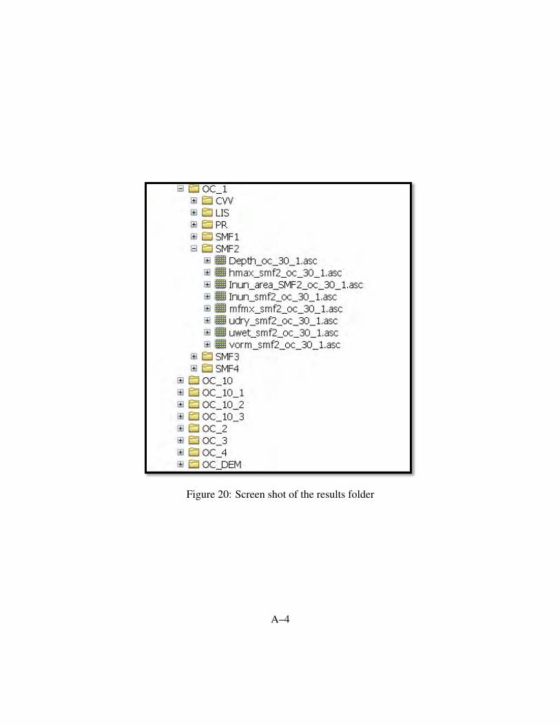
Figure 20: Screen shot of the results folder
A–4
Appendix B Modeling inputs
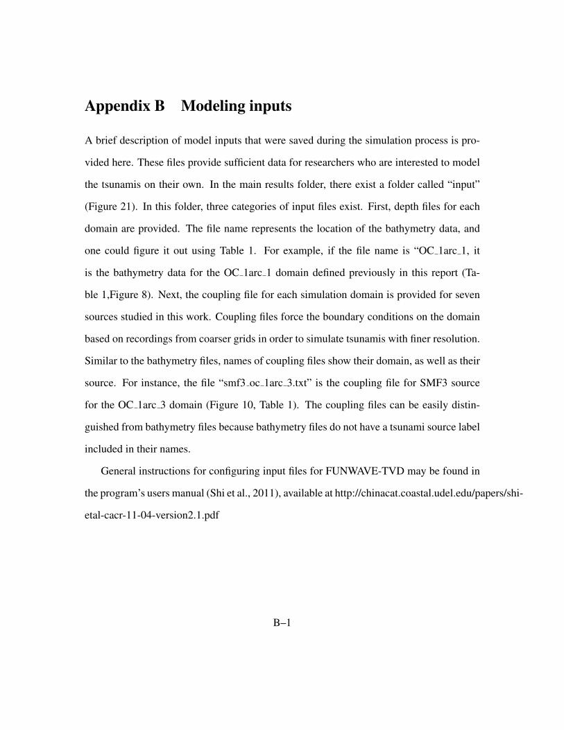
A brief description of model inputs that were saved during the simulation process is pro-
vided here. These files provide sufficient data for researchers who are interested to model
the tsunamis on their own. In the main results folder, there exist a folder called “input”
(Figure 21). In this folder, three categories of input files exist. First, depth files for each
domain are provided. The file name represents the location of the bathymetry data, and
one could figure it out using Table 1. For example, if the file name is “OC 1arc 1, it
is the bathymetry data for the OC 1arc 1 domain defined previously in this report (Ta-
ble 1,Figure 8). Next, the coupling file for each simulation domain is provided for seven
sources studied in this work. Coupling files force the boundary conditions on the domain
based on recordings from coarser grids in order to simulate tsunamis with finer resolution.
Similar to the bathymetry files, names of coupling files show their domain, as well as their
source. For instance, the file “smf3 oc 1arc 3.txt” is the coupling file for SMF3 source
for the OC 1arc 3 domain (Figure 10, Table 1). The coupling files can be easily distin-
guished from bathymetry files because bathymetry files do not have a tsunami source label
included in their names.
General instructions for configuring input files for FUNWAVE-TVD may be found in
the program’s users manual (Shi et al., 2011), available at http://chinacat.coastal.udel.edu/papers/shi-
etal-cacr-11-04-version2.1.pdf
B–1
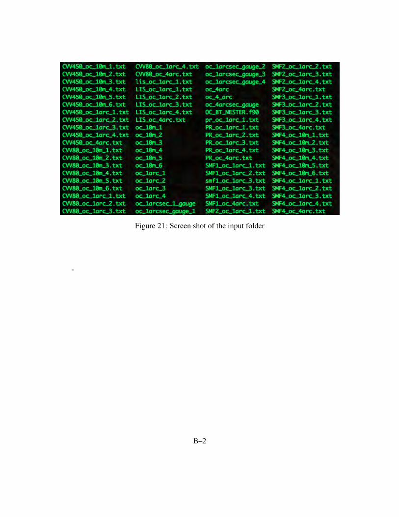
Figure 21: Screen shot of the input folder
-
B–2
Appendix C Inundation Mapping Guidelines
The development of inundation maps for tsunami hazard assessment and evacuation plan-
ning is governed by three documents and a related appendix. These include:
1. NTHMP Inundation Modeling Guidelines
Available at: http://nws.weather.gov/nthmp/modeling guidelines.html
2. Mapping Guidelines Appendix A
Available at: http://nws.weather.gov/nthmp/documents/MnM guide appendix-final.docx
3. NTHMP Tsunami Evacuation Mapping Guidelines
Available at: http://nws.weather.gov/nthmp/documents/NTHMPTsunamiEvacuationMappingGuidelines.pdf
4. NTHMP Guidelines for Establishing Tsunami Areas of Inundation for Non-Modeled
or Low-Hazard Areas
Available at: http://nws.weather.gov/nthmp/documents/Inundationareaguidelinesforlowhazardareas-
Final092611.docx
C–1