observing the continental-scale carbon balance: … · 2school of earth sciences, university of...

Atmos. Chem. Phys., 12, 7867–7879, 2012www.atmos-chem-phys.net/12/7867/2012/doi:10.5194/acp-12-7867-2012© Author(s) 2012. CC Attribution 3.0 License.

AtmosphericChemistry

and Physics

Observing the continental-scale carbon balance: assessment ofsampling complementarity and redundancy in a terrestrialassimilation system by means of quantitative network design

T. Kaminski 1, P. J. Rayner2, M. Voßbeck1, M. Scholze3, and E. Koffi4

1FastOpt, Lerchenstraße 28a, 22767 Hamburg, Germany2School of Earth Sciences, University of Melbourne, Melbourne, Australia3Dept. of Earth Sciences, University of Bristol, Bristol, UK4LSCE/IPSL, Gif-sur-Yvette Cedex, France

Correspondence to:T. Kaminski ([email protected])

Received: 29 February 2012 – Published in Atmos. Chem. Phys. Discuss.: 12 March 2012Revised: 31 July 2012 – Accepted: 17 August 2012 – Published: 31 August 2012

Abstract. This paper investigates the relationship betweenthe heterogeneity of the terrestrial carbon cycle and the op-timal design of observing networks to constrain it. We com-bine the methods of quantitative network design and carbon-cycle data assimilation to a hierarchy of increasingly hetero-geneous descriptions of the European terrestrial biosphere asindicated by increasing diversity of plant functional types.We employ three types of observations, flask measurementsof CO2 concentrations, continuous measurements of CO2and pointwise measurements of CO2 flux. We show that fluxmeasurements are extremely efficient for relatively homoge-neous situations but not robust against increasing or unknowncomplexity. Here a hybrid approach is necessary, and we rec-ommend its use in the development of integrated carbon ob-serving systems.

1 Introduction

CO2 and methane are the most important anthropogenicgreenhouse gases. Their increasing concentration is the ma-jor reason for global warming (Solomon et al., 2007). It isthus of paramount interest to quantify and ultimately pre-dict the exchanges of these gases between the terrestrial bio-sphere and the atmosphere. At a number of points on theglobe, carbon and water fluxes are sampled directly (see,e.g.http://www.fluxnet.ornl.gov). The interpolation of thesemeasurements to the globe (upscaling) requires external in-

formation about the uncertain spatio-temporal flux structure.The same type of information is required by atmospherictransport inversions (see e.g.Rayner et al., 1999; Gurneyet al., 2002; Enting, 2002) which infer surface fluxes fromatmospheric concentration measurements. The most sophis-ticated tools for quantifying the structure and variability ofcarbon fluxes are process models of the terrestrial carbon cy-cle like those used for the assessments of the IPCC (Solomonet al., 2007). Underlying these models is the assumption offundamental equations that govern the processes controllingthe terrestrial carbon fluxes. Uncertainty in the simulation ofthese fluxes arises from four sources: first, there is uncer-tainty in the forcing data (such as precipitation or temper-ature) driving the terrestrial processes. Second, there is un-certainty regarding the formulation of individual processesand their numerical implementation (structural uncertainty).Third, there are uncertain constants (process parameters) inthe formulation of these processes (parametric uncertainty).Forth, there is uncertainty about the state of the terrestrialbiosphere at the beginning of the simulation.

Observational information helps to reduce these uncer-tainties. Currently there are several initiatives to extend theobservational network of the carbon cycle. Europe’s Inte-grated Carbon Observing System (ICOS, seehttp://www.icos-infrastructure.eu/), for example, aims at setting up an in-tegrated sampling network for land, ocean, and atmosphere.Ideally, all data streams are interpreted simultaneously withthe process information provided by the model to yield a

Published by Copernicus Publications on behalf of the European Geosciences Union.

http://www.fluxnet.ornl.gov

http://www.icos-infrastructure.eu/

http://www.icos-infrastructure.eu/

7868 T. Kaminski et al.: Observing the continental-scale carbon balance

consistent picture of the carbon cycle that balances all the ob-servational constraints, thereby taking the respective uncer-tainty ranges into account. Data assimilation systems aroundprognostic models of the carbon cycle are the ideal tools forthis integration allowing us to assimilate a wide range ofobservations. They can, for example, be applied to system-atically reduce parametric uncertainty (e.g.Kaminski et al.,2002) or to expose structural errors (Rayner, 2010). In a firststep, they use the observations to constrain the uncertain pro-cess parameters (calibration), and in a second step they usethe calibrated model for analysis and prediction. Ideally, bothsteps include the propagation of uncertainties. This allows usto derive uncertainty ranges on simulatedtarget quantitiesthat are consistent with the uncertainties in the observationsand the model. Examples of such target quantities are fluxesof carbon on regional, continental, or global scale, integratedover part of the assimilation period (diagnostic target quan-tity) or some period before or after (prognostic target quan-tity). With regard to a specified target quantity, such an as-similation system can assess the performance of a given ob-servational network. This performance is typically quantifiedby the uncertainty range.

Quantitative Network Design (QND) aims at constructingan observational network with optimal performance. The ap-proach is based onHardt and Scherbaum(1994) who op-timised the station locations for a seismographic network.It was first applied to observational networks of the globalcarbon cycle byRayner et al.(1996), who optimised thelocations of atmospheric CO2 and δ13C measurements. Apioneering study for sensor design has been performed byRayner and O’Brien(2001) who established the required pre-cision for observations of the column-integrated atmosphericCO2 concentration from space.

The latter two studies investigated purely atmospheric net-works. To assist the design of an integrated carbon observingsystem, we need the capability of evaluating the complemen-tarity of various observational data streams including thoseof the terrestrial biosphere. As outlined byKaminski andRayner(2008) assimilation systems are the ideal tool for thistask. The Carbon Cycle Data Assimilation System (CCDAS,seehttp://ccdas.org) can assimilate several observational datastreams and infers uncertainty ranges on diagnosed (Rayneret al., 2005) or prognosed carbon (Scholze et al., 2007;Rayner et al., 2011) and water (Kaminski et al., 2012) fluxes.The first QND applications investigated the utility of spaceborne observations of atmospheric CO2 (Kaminski et al.,2010) or vegetation activity (Kaminski et al., 2012) in con-straining various surface fluxes. Another study explores theatmospheric in situ network and its ability to constrain theproductivity of the terrestrial biosphere (Koffi et al., 2012).

Kaminski and Rayner(2008) noted two general aspects ofQND studies. The first is the dependence on the target quan-tity; clearly different networks are optimal for constrainingdifferent things (Rayner et al., 1996). The second is the de-pendence on prior knowledge brought to the problem. For

traditional inversions of fluxes this information takes theform of the covariance of prior uncertainty. For CCDAS itis determined by the process resolution of the underlying dy-namical model (how many processes are modelled) and thespatial detail at which these processes are allowed to vary in-dependently. The level of heterogeneity of the biosphere isa fundamental question which goes beyond CCDAS; it de-termines how much any understanding of processes gainedlocally can be more widely applied. However it is clear thatobserving networks presupposing a given heterogeneity areat some risk. Current earth system models map this spatialheterogeneity by dividing the global vegetation into a smallnumber of plant functional types (PFTs).Groenendijk et al.(2011) demonstrate through calibration of a terrestrial modelagainst direct flux measurements the limit of this approxima-tion and the difficulty in deriving a realistic PFT classifica-tion.

This paper uses the network designer, a CCDAS-based in-teractive QND tool, to investigate the performance of severalnetworks composed of direct flux observations and flask orcontinuous samples of the atmospheric carbon dioxide con-centration. In particular we investigate the robustness of net-work performance to various choices of target quantities andlevels of heterogeneity. The outline of the paper is as fol-lows. Section2 describes our QND methodology and Sect.3the networks we consider. Then Sect.4 will present and dis-cuss the evaluations. Finally, in Sect.5 we summarise ourconclusions.

2 Methods

CCDAS is built around the Biosphere Energy Transfer HY-drology scheme (BETHY,Knorr, 2000; Knorr and Heimann,2001), a global model of the terrestrial vegetation. The ver-sion used here is described inRayner et al.(2005). This sec-tion gives brief descriptions of BETHY, the observationaldata types, CCDAS and of the QND approach.

2.1 BETHY

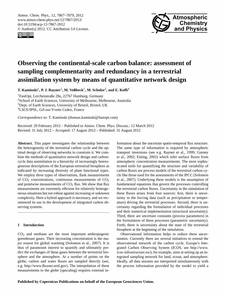
FollowingWilson and Henderson-Sellers(1985) BETHY de-composes the global terrestrial vegetation into 13 PFTs aslisted in Table1. Each grid cell can be covered by up to threePFTs. Figure1 shows the distribution of the dominant PFT.As in Scholze et al.(2007) we integrate the model over 21 yrfrom 1979 to 1999 on a global 2 by 2 degree grid and useobserved meteorological driving data (Nijssen et al., 2001).

The process formulations within BETHY are controlledby a set of process parameters (see Table2). For this studywe use the model version ofScholze et al.(2007) with theextension of simulating hourly Net Ecosystem Productivity(NEP). This is done by dividing the daily calculated het-erotrophic respiration flux into 24 equal-sized hourly fluxesand subtracting these fluxes from the hourly simulated Net

Atmos. Chem. Phys., 12, 7867–7879, 2012 www.atmos-chem-phys.net/12/7867/2012/

http://ccdas.org

T. Kaminski et al.: Observing the continental-scale carbon balance 7869

Table 1. Plant Functional Types (PFTs) defined in CCDAS and their abbreviations, taken from Rayner et al.

(2005).

PFT No. PFT Name Abbreviation

0 Not vegetated

1 Trop. broadleaved evergreen tree TrEv

2 Trop. broadleaved deciduous tree TrDec

3 Temp. broadleaved evergreen tree TmpEv

4 Temp. broadleaved deciduous tree TmpDec

5 Evergreen coniferous tree EvCn

6 Deciduous coniferous tree DecCn

7 Evergreen shrub EvShr

8 Deciduous shrub DecShr

9 C3 grass C3Gr

10 C4 grass C4Gr

11 Tundra vegetation Tund

12 Swamp vegetation Wetl

13 Crops Crop

Fig. 1. Distribution of the dominant CCDAS Plant Functional Type (PFT) per grid cell, PFT labels are given in

Table 1, taken from Rayner et al. (2005).

18

Fig. 1. Distribution of the dominant CCDAS Plant Functional Type (PFT) per grid cell, PFT labels are given in Table1, taken fromRayneret al.(2005).

Table 1.Plant Functional Types (PFTs) defined in CCDAS and theirabbreviations, taken fromRayner et al.(2005).

PFT No. PFT Name Abbreviation

0 Not vegetated1 Trop. broadleaved evergreen tree TrEv2 Trop. broadleaved deciduous tree TrDec3 Temp. broadleaved evergreen tree TmpEv4 Temp. broadleaved deciduous tree TmpDec5 Evergreen coniferous tree EvCn6 Deciduous coniferous tree DecCn7 Evergreen shrub EvShr8 Deciduous shrub DecShr9 C3 grass C3Gr10 C4 grass C4Gr11 Tundra vegetation Tund12 Swamp vegetation Wetl13 Crops Crop

Primary Productivity (NPP). BETHY simulates 13 PFTs in-cluding 21 different parameters. Three of these parametersare PFT-specific and 18 are applied globally, i.e. they refer toall PFTs. We thus have 18+3×13= 57 parameters. The roleof the individual parameters is described elsewhere (Rayneret al., 2005; Scholze et al., 2007). In our context of networkdesign it is important to know to which parameters our re-spective target quantities are sensitive. We will use regionalintegrals of the NPP and the NEP as target quantities. The lat-ter is net CO2 flux between the atmosphere and the biosphereand defined as the difference of NPP and heterotrophic soilrespiration. Except for one atmospheric parameterc0, all pa-rameters impact NEP. NPP is sensitive to all parameters, ex-ceptc0 and the soil and carbon balance parameters.

2.2 Observational data types

In this study we use three types of observational data: di-rect (NEP) flux measurements, flask and continuous samplesof the atmospheric CO2 concentration. Within the model, aflux measurement is represented by a time series of hourlyNEP samples of the grid cell the site is located in. The atmo-spheric data types require, as a so-called observation opera-tor, an atmospheric transport model to transform the globalNEP field into atmospheric concentrations. Flask samplesare represented by a time series of monthly mean concen-trations at the sampling location as simulated by the atmo-spheric transport model TM2 (Heimann, 1995), which is runat 8 by 10 degree horizontal resolution and with nine verti-cal levels. As inCarouge et al.(2010a,b) continuous sam-ples are represented by a time series of daily mean concen-trations at the sampling location as simulated by the atmo-spheric transport model LMDZ (Hauglustaine et al., 2004),which is run at 3.75 by 2.5 degree resolution over most ofthe globe but a zoomed 0.5 degree resolution over Europe.For each data type the observational time series covers the20 yr period from 1980 to 1999. By representing flask sam-ples in the model as monthly means, much of the synopticsignal is averaged out. Likewise by representing continuousmeasurements by daily means the diurnal signal is averagedout. This averaging reduces the information content of theobservations but is also less demanding of the models’ per-formance, i.e. a conservative choice. A model setup with en-hanced temporal representation of the flask or continuousdata types would probably provide stronger constraints onthe target quantities.

2.3 CCDAS

CCDAS uses a gradient method to adjust BETHY’s pro-cess parameters in order to minimise a cost function. Thiscost function quantifies the fit to all observations plus the

www.atmos-chem-phys.net/12/7867/2012/ Atmos. Chem. Phys., 12, 7867–7879, 2012


deviation from prior knowledge on the process parameters:

J (x) =1

2

[(M(x) − d)T C(d)−1(M(x) − d)

+(x − x0)T C(x0)

−1(x − x0)]

(1)

whereM denotes the model considered as a mapping fromparameters to observations,d the observations with data un-certainty C(d), x0 the prior parameter values with uncer-taintyC(x0), and the superscriptT the transpose.

The second derivative (Hessian) of the cost function at theoptimumx is used to approximate the inverse of the covari-ance matrixC(x) that quantifies the uncertainty ranges on theparameters that are consistent with uncertainties in the obser-vations and the model. In a second step, the linearisationN ′

(Jacobian) of the modelN used as a mapping from param-eters to target quantities is used to propagate the parameteruncertainties forward to the uncertainty in a target quantityσ(y):

σ(y)2= N ′C(x)N ′T

+ σ(ymod)2 . (2)

σ(ymod) quantifies all uncertainty in the simulation of the tar-get quantity except the uncertainty inx (which we resolve ex-plicitly). If the terrestrial model was perfect,σ(ymod) wouldbe zero. In contrast, if the parameters were perfectly known,the first term on the right hand side would be zero. Likewisethe data uncertaintyC(d) is the sum of the observational un-certainty and all uncertainty in the simulation of the observa-tions except the uncertainty in the parameter vector.

All derivative information is provided with the same nu-merical accuracy as the original model in an efficient formvia automatic differentiation of the model code by the auto-matic differentiation tool TAF (Giering and Kaminski, 1998).

2.4 QND

In network design mode, CCDAS is restricted to the uncer-tainty propagation for candidate networks. It builds on theoptimal parameter set estimated from data of the availablenetwork for the evaluation of the required first and secondderivatives. In our case the optimal parameter vector is takenfrom the study ofScholze et al.(2007). For the evaluation ofpotential networks, the Hessian is evaluated ford = M(x).In this case the posterior target uncertainty solely dependson the prior and data uncertainties and linearised model re-sponses at observational locations and for target quantities.The approach does not require real observations, and can thusevaluate hypothetical candidate networks (seeKaminski andRayner, 2008; Kaminski et al., 2010). Candidate networksare defined by a set of observations characterised by observa-tional data type, location, and data uncertainty. In practise forpre-defined target quantities and observational types and lo-cations, model sensitivities can be pre-computed and stored.A network composed of these pre-defined observations, canthen be evaluated in terms of the pre-defined target quanti-ties without further model evaluations. Only matrix algebra

is required to combine the pre-computed sensitivities withthe data uncertainties.

This is the approach implemented in the network de-signer (seehttp://imecc.ccdas.org), an interactive softwaretool that evaluates networks composed of flask and contin-uous samples of atmospheric CO2 and direct flux measure-ments. Available target quantities are NPP and NEP overthree regions: Europe, Brazil, and Russia (see Fig.2). Theyare provided in the form of annual mean values averaged overthe 20 yr assimilation period. Model sensitivities have beenpre-computed for a list of atmospheric sampling sites (seeFig. 3 and Table4). For flux measurements, model sensitivi-ties have been pre-computed for every terrestrial grid cell andall PFTs that are available in the grid cell. When defining thesite, the user can specify a mix among these PFTs. Uncertain-ties for data sampled at different sites and times are assumedto be uncorrelated. The uncertainty for each site is quanti-fied by a standard deviationσ(d), that reflects the combinedeffect of observationalσ(dobs) and model errorσ(dmod):

σ(d)2= σ(dobs)

2+ σ(dmod)

2 (3)

The unit of the data uncertainties depends on the data type.For flask and continuous samples of atmospheric CO2 it isppm, for eddy flux measurements it is gCm−2day−1 (wheregC stands for grams of carbon). The output of the networkdesigner is the list of posterior uncertaintiesσ(y) of the targetquantities according to Eq. (2). σ(ymod) can be specified bythe user as a percentage of the 20 yr average of annual meanNPP.

3 Experimental setup

We will be evaluating several networks. To define these net-works we have to select the sampling locations and the re-spective data uncertainties. Data uncertainty is generally dif-ficult to estimate, especially in advance of actual measure-ments. In the following we give some motivation for ourchoices and for some cases we will test the effect of an al-ternative choice in Sect.4.

The thrust of our study is the interaction between the spa-tial density of various classes of measurements and assumedheterogeneity of the spatial biosphere. It is important there-fore that our choice of data uncertainty does not overly in-fluence the results. We therefore make the most neutral pos-sible choice of a uniform data uncertainty for each class ofmeasurement. We also assume uncorrelated uncertainties inspace and time. This is partly justified by the reduction inthe underlying datasets to either daily or monthly means and,more importantly, by the focus of our study. We note that,in principle, systematic errors (biases) in the observations orthe model (which would give rise to uncertainty correlationsalong the entire time series) can be removed or at least re-duced by bias correction schemes. For example,Pillai et al.


http://imecc.ccdas.org


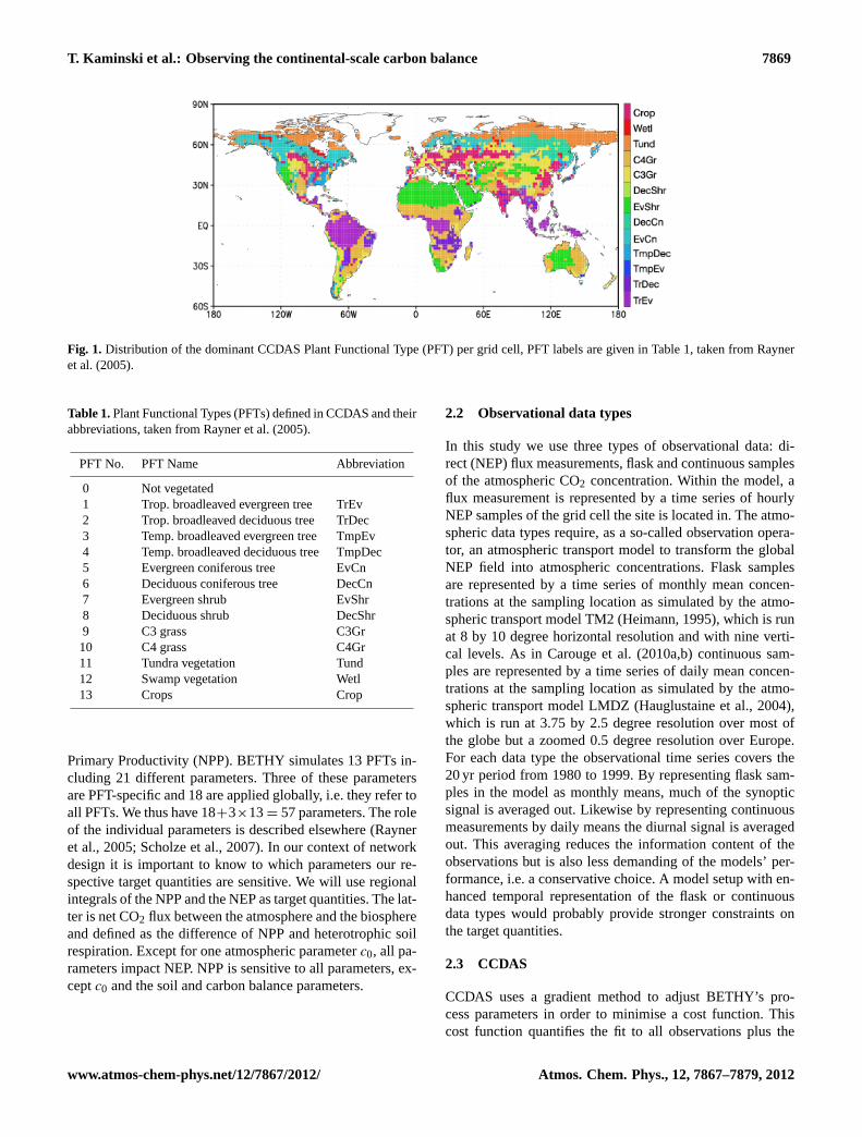
Fig. 2. Regions for computation of target quantities: grid cells contributing to fluxes over Europe (blue), Russia (red), both (violet), andBrazil (green).

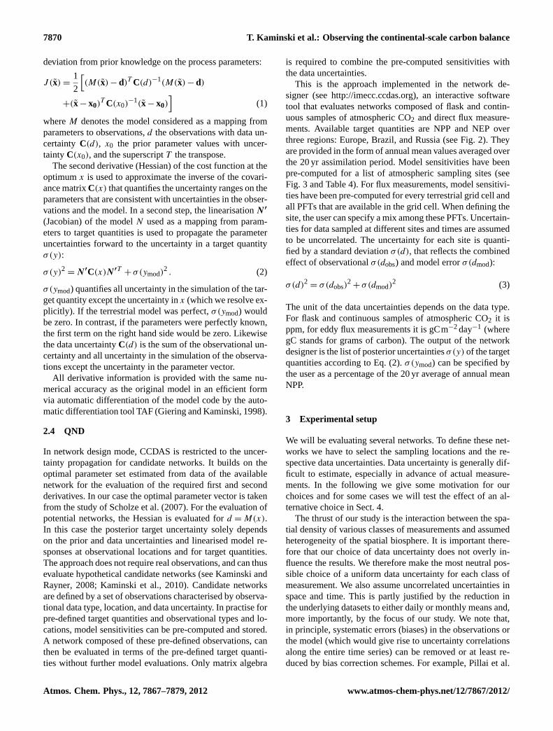
Fig. 3.Observational networkflaskproviding atmospheric flask samples.

(2010) assess biases for the atmospheric data types and de-rive a recipe for their reduction.

For the flux measurements we use an uncertainty of10 gCm−2day−1. With respect to the minimum uncer-tainty of 3× 10−6molm−2s−1

≈ 3.11gCm−2day−1 chosenby Knorr and Kattge(2005) this is a factor of about

√10

larger. This effective sample size of 10 corresponds to ignor-ing half of the data because of nighttime sampling and allow-ing another factor of 5 to account of correlated uncertainties.

For the atmospheric data types we assume the combinederror in the terrestrial and transport models to be the domi-

nant contribution to data uncertainty. For flask samples (rep-resented by monthly mean values) we use a data uncertaintyof 1.0 ppm, above the average assigned byRodenbeck et al.(2003) for the combined observational and transport modelerror. For continuous observations, which are more difficultto simulate, we use an uncertainty of 1.5 ppm. We can regardthe factor of 1.5 compared to flask samples as an inflation ofthe data uncertainty, to achieve an effective sample size thatis reduced by a factor of 2. With roughly 30 times as manymeasurements this still gives continuous observations greater



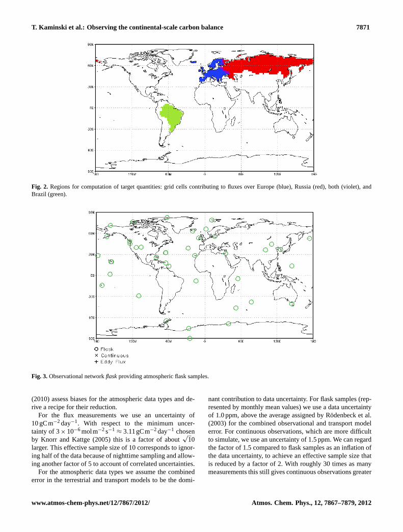
Fig. 4.Observational networksflux (+) providing flux measurements andcont (X) providing continuous atmospheric samples.

weight than flask measurements but this is reasonable giventheir greater ability to represent a monthly mean.

Next we have to define the sampling locations. For eachobservational data type we define a base network:

– The atmospheric flask sampling networkflask, whichconsists of the 41 monitoring stations listed in Table 2of Kaminski et al.(2002) and shown in Fig.3.

– The atmospheric continuous sampling networkcont,which consists of the 15 sites listed in Table4 and indi-cated with symbol “X” in Fig.4.

– The eddy flux networkflux, which consists of a dedi-cated site for each of the ten PFTs that are available tothe model over Europe (PFT numbers 3–5 and 7–13 ofTable1). Each site is defined such that it is covered to100 % by the respective PFT. Table3 lists the sites andFig. 4 indicates their locations with the symbols “+”.

We evaluate the networks in terms of the uncertainty re-duction (Kaminski et al., 1999) in six target quantities:

1−σ(y)

σ (yprior), (4)

whereσ(yprior) denotes the uncertainty in the target quantitywithout any observational constraint andσ(y) is taken fromEq. (2). The prior uncertainties for our target quantities arecomputed by propagating the prior parameter uncertaintiesof Scholze et al.(2007) via the JacobianN ′ (Eq. 2). They

are 0.45 GtC, 1.45 GtC, and 1.13 GtC for NEP over Europe,Russia, and Brazil, respectively, and 0.66 GtC, 1.08 GtC, and4.86 GtC for NPP.σ(ymod) is an offset in Eq. (2). If the termwas very high it would dominate the posterior uncertainty. Torender the contrasts between the networks more drastic, weuse a value of zero, i.e. we only analyse the effect of the net-works on the parametric uncertainty in the target quantities.In fact, some of the parameters rather refer to the initial state,i.e. this source of uncertainty is also covered, to a limitedextent, by our analysis.

In the above-described default set up BETHY runs with13 PFTs. To investigate the robustness of the network per-formance with respect to model complexity in terms of thenumber of available PFTs, we extend the default set up asfollows: we split the global vegetation into several equal frac-tions. Each fraction has its own set of 57 independent param-eters with uncorrelated prior uncertainty. All fractions of aPFT share the location of the original PFT. In other words,a grid cell that in the default setup is populated by a singlePFT is now composed of equal subgrid patches, each withtheir own PFT; the corresponding surface fluxes add up toone grid cell flux to be used for the atmospheric networks(hence the patches can be said to have the same location)but they are separately monitored by the flux network. In thefollowing we will call the number of fractionsmultiplicity.With multiplicity 4, for example, we have 4× 13= 52 PFTsand 57× 4 = 228 parameters. A parameter that was globalin the default configuration now has its validity restrictedto one of the fractions of the global vegetation. A change



Table 2.Process parameters, their symbols (2nd column), their description (3rd column), whether their scope is PFT specific or global (4thcolumn), whether NEP (5th column) or NPP (6th column) are sensitive to them.

Number Symbol Description scope NEP NPP

1 V 25max maximum carboxylation rate (C3) PFT X X

2 aJ,V ratioV 25max over max electron transportJ25

max PFT X X3 αq photon capture efficiency (C3) global X X4 αi quantum efficiency (C4) global X X5 K25

C Michaelis-Menten constant CO2 global X X6 K25

O Michaelis-Menten constant O2 global X X7 a0,T temperature slope CO2 compensation point global X X8 EKO activation energy, O2 global X X9 EKC activation energy, CO2 global X X10 EVmax activation energy, carboxylation rate (C3) global X X11 Ek activation energy, carboxylation rate (C4) global X X12 ERd activation energy, dark respiration global X X13 fR,leaf leaf respiration ratio global X X14 fR,growth growth respiration ratio global X X15 fS fraction of fast soil decomposition global X16 κ soil moisture exponential for soil respiration global X17 Q10,f soil respiration temperature factor, fast pool global X18 Q10,s soil respiration temperature factor, slow pool global X19 τf fast pool soil carbon turnover time global X20 β net CO2 sink factor PFT X21 c0 atmospheric concentration offset global

Table 3. Network flux. First number in site name indicates modelgrid cell and second number PFT.

Name Included Uncertainty lon lat[gCm−2day−1]

site1413-3 yes 10.0 9.0 45.0site1025-4 yes 10.0 35.0 53.0site143-5 yes 10.0 19.0 69.0site148-7 yes 10.0 29.0 69.0site1495-8 yes 10.0 −5.0 43.0site1731-9 yes 10.0 −5.0 37.0site1578-10 yes 10.0 −5.0 41.0site377-11 yes 10.0 −21.0 65.0site388-12 yes 10.0 29.0 65.0site621-13 yes 10.0 13.0 61.0

of multiplicity also affects the prior uncertainty in the tar-get quantities. Introducing the multiplicitym means thatmcopies have to share the same area. Hence, compared to theoriginal flux y the flux yi from each copy (i counting thecopies) is reduced by a factor ofm. And with it the origi-nal flux uncertaintyσ(yprior) is also reduced by a factor ofm

for each copyσ(yi,prior). Since there is no correlation of theprior uncertainty among the copies, the total flux uncertaintyσ(yprior,m) is the square root of the sum of squares:

Table 4. Network cont of continuous atmospheric sampling sitesover Europe.

Name Included Uncertainty lon lat[ppm]

CBW yes 1.5 4.9 52.0CMN yes 1.5 10.7 44.1DGR yes 1.5 22.07 54.15FDA yes 1.5 25.3 45.47HUN yes 1.5 16.6 46.9MHD yes 1.5 −9.9 53.33NGB yes 1.5 13.05 53.15PAL yes 1.5 24.12 67.97PRS yes 1.5 7.7 45.9PUY yes 1.5 3.0 45.8SAC yes 1.5 2.2 48.7SBK yes 1.5 12.98 47.05SCH yes 1.5 8.0 48.0WES yes 1.5 8.0 55.0WHF yes 1.5 10.77 52.8

σ(yprior,m) =

√ ∑i=1,m

σ(yi,prior)2 =

√ ∑i=1,m

(σ (yprior)

m)2

=σ(yprior)

√m

. (5)



Fig. 5.Evaluation of two flux sites (blue and orange bars), of their combination (yellow bars), and of each site with data uncertainty reducedby a factor of 100 (green and brown bars): Uncertainty reduction for NEP and NPP integrated over three regions.

This means, for example, quadrupling the multiplicity halvesthe prior uncertainty.

4 Results and discussion

We start this section with evaluations of simple networkscomposed of one or two flux sites. Then we move on to thebase networks defined in Sect.3 and, finally, study the effectof increasing the number of PFTs that are available to themodel.

4.1 Simple configurations of flux sites

The selection of a site location for sampling a particular PFTdefines the Jacobian matrix that provides the link from themodel parameters (required for simulating that PFT) to thesimulated flux. To understand the effects which we will latersee in larger networks, it is instructive to evaluate first a seriesof small networks consisting of one or two flux sites. We startwith the separate evaluation of two sites which both observePFT 9 (C3 grass) to 100 %, namely “site1731-9” in SouthernSpain and “site143-9” in Northern Scandinavia. Note that wecan populate any given location with up to three PFTs. Forthe current experiment we take the location of “site143-5”from Table3 but populate it to 100 % with PFT 9. For conve-nience, for the remainder of this subsection, we will refer tothe sites just as “143” and “1731”. The respective uncertaintyreductions are displayed by blue (site “143”) and orange (site“1731”) bars in Fig.5. First we note that flux measurementsover Europe can reduce the uncertainty of target quantitiesover Russia and Brazil. This reflects our assumption of fun-damental processes with a combination of universal and PFT-specific parameters: an observation provides information be-yond its sampling time and location helping to reduce un-certainty everywhere. Figure6 shows for site “1731” the un-certainty reduction in NEP per grid cell. This quantifies howthe observational information of the site is spread around the

globe. Comparing with Fig.1 we note high uncertainty re-duction where the dominant PFT is C3 grass.

Among the two sites in terms of NEP site “1731” performsonly marginally better, but in terms of NPP it performs about10 percentage points better1. Next we investigate the com-plementarity between the two sites, i.e. we use a network thatconsists of both sites and note a slight improvement for NPPover Europe and Russia (yellow bar in Fig.5) compared tothe better site “1731” alone. For these two target quantitiesthe weaker site “143” is notredundantin this two site net-work, because it brings at least a little bit of extra informa-tion. In other words there is at least a slightcomplementaritybetween the two sites with respect to the two target quanti-ties.

For the analysis of the above effects, recall that each scalartarget quantity is (through the vectorN ′ of Eq. 2) influ-enced by its own one-dimensional sub-space of the parame-ter space, i.e. atarget directionin parameter space. Likewiseeach scalar observation constrains a direction in parameterspace (observed direction). We can use the analogy of aper-spectiveunder which the target direction is observed. If thetarget and observed directions are orthogonal, the observa-tion can not reduce the uncertainty in the target quantity. Ifboth directions are collinear, i.e. in the same subspace of theparameter space, the observation can most efficiently reducethe uncertainty in the target quantity. This means, for exam-ple, that even a hypothetically perfect measurement that re-moved all uncertainty for all parameters pertinent to one PFTwould not completely constrain any of our target quantities(which are all influenced by several PFTs). In other words aone-site flux network isincompletewith respect to our targetquantities. The strength of an observational constraint on atarget quantity depends (1) on the sensitivity of the observed

1The unitpercentage pointquantifies an absolute change in thepercentage value. For example, for a value of 40 % an increase by50 percentage points yields 90 %. By contrast, an increase by 50 %corresponds to 20 percentage points and yields 60 %.



Fig. 6.Uncertainty reduction in NEP per grid cell, for a network consisting of a single flux site (site 1731-9 in Table4).

quantity to a parameter change in the observed direction (sig-nal size), (2) on how well the observed direction projects ontothe target direction (perspective), and (3) on the data uncer-tainty. We use the same data uncertainty for both sites andthe same target directions. The observed direction and signalsize depend (1) on the PFT, (2) on the sampling time, and on(3) the meteorological driving data. Our two flux sites pro-vide measurements at the same times (hourly for 20 yr) andof the same PFT. The only different factors are the meteo-rological driving data. Indeed the meteorology in SouthernSpain is quite different from Scandinavia.

To isolate the effects of the perspective and the signal sizeon performance of the individual sites we reduce their respec-tive data uncertainties by a factor of 100 (green and brownbars in Fig.5). This can compensate for a weaker signal butdoes not change the perspective. Now both sites show ex-actly the same performance, i.e the Scandinavian site has justa smaller signal. In other words, we find the relevant infor-mation at both sites, but at sites with a larger signal we canafford a larger data uncertainty or, probably, a shorter obser-vational period.

A common property between all networks evaluated inFig.5 is the larger uncertainty reduction for NPP compared toNEP. This happens although we sample hourly NEP, i.e. weshould match the perspective for long-term NEP quite well.On the other hand, the target space for NPP has fewer di-mensions, because it depends on fewer parameters. The extraparameters in NEP play an important role. This effect wouldprobably be even more pronounced if NEP was comparedwith the Gross Primary Productivity (GPP) which is influ-enced by even fewer parameters (Koffi et al., 2012). Another

point to note is that for Brazil the prior uncertainty in NPPis about four times higher than for NEP, and thus easier toreduce.

4.2 Base networks and their combinations

The performance of the three base networksflask(blue bars),cont (orange bars), andflux (yellow bars) is shown in Fig.7.Over Europe, the flux network achieves an uncertainty reduc-tion of about 99 % for both NEP and NPP and outperformsboth atmospheric networks. The reason for the strong perfor-mance offlux over Europe is its completeness with respectto the European target quantities, i.e. the fact that for eachPFT over Europe it contains a dedicated site. With respect tothe Brazilian target quantities, in turn, the networkflux is in-complete because it does not cover the tropical PFTs. This iswhy flux is weaker than the global networkflask, in particu-lar for NEP where the performance difference between bothnetworks is over 50 percentage points.

The above suggests we would always attempt completeflux networks. In reality this will be hard to achieve, becausewe do not know how many PFTs are required to simulate theterrestrial carbon cycle, nor do we know their spatial distri-bution (Groenendijk et al., 2011). Hence, it may happen thatwe accidently miss a PFT in our flux network. We can test theeffect of this by removing from networkflux the site “1731-9” (networkflux-C3). The performance over Europe drops byabout 69 percentage points for NEP and 58 for NPP (greenbars). Over Brazil the effect of missing the C3 grass site isonly marginal (performance drop of less than four percent-age points for NEP and less than two for NPP).



Fig. 7.Evaluation of three base networks, a flux networkflux-C3that is incomplete over Europe and the combinedflux-C3+ flasknetwork.

For the atmospheric networks,flaskoutperformscontoverEurope by 2 and 10 percentage points for NEP and NPPdespite the European focus ofcont. Obviously, for the at-mosphere, the large-scale information matters. For Brazil orRussia it is not surprising that the global networkflask ismore powerful than the networkcont. The most important as-pect is that the atmospheric networks outperform the incom-plete flux networkflux-C3. The only exception is NPP overBrazil, where the loss of C3 had only a marginal effect onthe performance of the flux network andflux-C3 is strongerthancontbut not thanflask. We note that the relatively coarseresolution of TM2 may yield a slight overestimation in theintegrative capacity offlask. For any given monthly meansample, the higher resolution of LMDZ would resolve a finerinfluence structure (footprint) within the TM2 grid cells. Onthe other hand, our sampling period of 20 yr would probablyaverage out much of this time-dependent fine-scale structure,a mechanism that tends to increase the footprint. Over thatperiod, it is not clear, per se, which of the transport mod-els has a higher integrative capacity. We note, however, thatin an inversion study the use of a high resolution model isfavourable in order to minimise biases through resolution-dependent effects caused, e.g. by orography (see, e.g.Pillaiet al., 2010). Increasing the data uncertainty ofcontby a fac-tor of four (to a value comparable to the data uncertainty offlask) yields only small performance reductions of 3 percent-age points over Europe, 6–7 percentage points over Russiaand below one percentage point over Brazil (not shown).

To assess thecomplementarityof atmospheric and fluxnetworks, we combine the networksflux-C3andflask. OverEurope the resulting networkflux-C3 + flaskperforms almostas well as thecompleteflux networkflux, and over Brazil andRussia even better. Both networks (flux-C3andflask) com-plement each other. Given the experience from the two grasssites we evaluated initially (Sect.4.1), we can think of theatmospheric network as an observer of averages over multi-ple sites. We can regard its addition to the flux network as aninsurance against theincompletenessof the flux network.

What can we do in the case where we can not affordenough sites to sample all PFTs over our target region? Isit useful to have a flux site which observes two PFTs? Wetest this by removing the site “site1731-9” from the networkfluxand modify the PFT fractions at site “site143-9” to 50 %each for PFTs 5 and 9. This network has the same numberof sites asflux-C3but much better performance (not shown).Uncertainty reduction for NEP over Europe is 76 %, and forthe other target quantities the performance is only marginally(less than one percentage point) inferior toflux. This perfor-mance enhancement is based on the same principle as atmo-spheric sampling, the integration of a multi-PFT signal. Thisresult seems surprising. It arises from the ability of a longtime series to observe the different dynamics of the two un-derlying PFTs.

We can also investigate the complementarity of the basenetworks. Since the uncertainty reduction for the networkflux is above 99 % already, in this set of assessments werather quantify the performance gain by the reduction in pos-terior uncertainty relative to the posterior uncertainty offlux.Adding both atmospheric networks to networkflux reducesNEP uncertainty over Europe by over 30 % and NPP by20 %. For the other regions the effect is much larger (up to99 % reduction for NEP over Brazil).

4.3 Increased model complexity

The above network evaluations are based on the defaultmodel setup with 13 PFTs. In the following we investigatethe robustness of the results with respect to model complex-ity in terms of the number of available PFTs. To increase thenumber of PFTs we use the procedure described in Sect.3.

For multiplicity 4, Fig. 8 shows the performance of thethree base networks. Among the atmospheric networksflaskis superior tocont for all target quantities, except for NEPover Europe whereflaskis slightly inferior. The networkflux,in turn, is superior toflaskexcept for NEP over Brazil andRussia. We define the networkM4-1 flux, which is incom-plete over Europe, by excluding one parameter copy out of



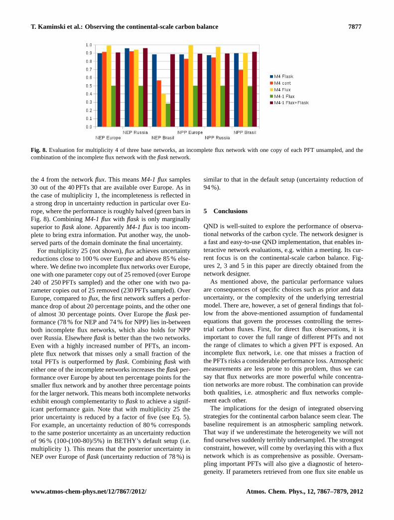
Fig. 8. Evaluation for multiplicity 4 of three base networks, an incomplete flux network with one copy of each PFT unsampled, and thecombination of the incomplete flux network with theflasknetwork.

the 4 from the networkflux. This meansM4-1 fluxsamples30 out of the 40 PFTs that are available over Europe. As inthe case of multiplicity 1, the incompleteness is reflected ina strong drop in uncertainty reduction in particular over Eu-rope, where the performance is roughly halved (green bars inFig. 8). CombiningM4-1 fluxwith flask is only marginallysuperior toflaskalone. ApparentlyM4-1 flux is too incom-plete to bring extra information. Put another way, the unob-served parts of the domain dominate the final uncertainty.

For multiplicity 25 (not shown),flux achieves uncertaintyreductions close to 100 % over Europe and above 85 % else-where. We define two incomplete flux networks over Europe,one with one parameter copy out of 25 removed (over Europe240 of 250 PFTs sampled) and the other one with two pa-rameter copies out of 25 removed (230 PFTs sampled). OverEurope, compared toflux, the first network suffers a perfor-mance drop of about 20 percentage points, and the other oneof almost 30 percentage points. Over Europe theflask per-formance (78 % for NEP and 74 % for NPP) lies in-betweenboth incomplete flux networks, which also holds for NPPover Russia. Elsewhereflaskis better than the two networks.Even with a highly increased number of PFTs, an incom-plete flux network that misses only a small fraction of thetotal PFTs is outperformed byflask. Combiningflask witheither one of the incomplete networks increases theflaskper-formance over Europe by about ten percentage points for thesmaller flux network and by another three percentage pointsfor the larger network. This means both incomplete networksexhibit enough complementarity toflaskto achieve a signif-icant performance gain. Note that with multiplicity 25 theprior uncertainty is reduced by a factor of five (see Eq.5).For example, an uncertainty reduction of 80 % correspondsto the same posterior uncertainty as an uncertainty reductionof 96 % (100-(100-80)/5%) in BETHY’s default setup (i.e.multiplicity 1). This means that the posterior uncertainty inNEP over Europe offlask(uncertainty reduction of 78 %) is

similar to that in the default setup (uncertainty reduction of94 %).

5 Conclusions

QND is well-suited to explore the performance of observa-tional networks of the carbon cycle. The network designer isa fast and easy-to-use QND implementation, that enables in-teractive network evaluations, e.g. within a meeting. Its cur-rent focus is on the continental-scale carbon balance. Fig-ures 2, 3 and 5 in this paper are directly obtained from thenetwork designer.

As mentioned above, the particular performance valuesare consequences of specific choices such as prior and datauncertainty, or the complexity of the underlying terrestrialmodel. There are, however, a set of general findings that fol-low from the above-mentioned assumption of fundamentalequations that govern the processes controlling the terres-trial carbon fluxes. First, for direct flux observations, it isimportant to cover the full range of different PFTs and notthe range of climates to which a given PFT is exposed. Anincomplete flux network, i.e. one that misses a fraction ofthe PFTs risks a considerable performance loss. Atmosphericmeasurements are less prone to this problem, thus we cansay that flux networks are more powerful while concentra-tion networks are more robust. The combination can provideboth qualities, i.e. atmospheric and flux networks comple-ment each other.

The implications for the design of integrated observingstrategies for the continental carbon balance seem clear. Thebaseline requirement is an atmospheric sampling network.That way if we underestimate the heterogeneity we will notfind ourselves suddenly terribly undersampled. The strongestconstraint, however, will come by overlaying this with a fluxnetwork which is as comprehensive as possible. Oversam-pling important PFTs will also give a diagnostic of hetero-geneity. If parameters retrieved from one flux site enable us



to predict the fluxes at a second then these are properly con-sidered the same PFT for CCDAS, otherwise we need to in-crease the multiplicity.

The above assumption of fundamental equations that gov-ern the processes controlling the terrestrial carbon fluxesdoes not apply to atmospheric transport inversions, whichhas an effect on the optimal sampling strategy. For example,transport inversions can incorporate the response of the car-bon fluxes to a difference in climate only to a limited extentthrough their prior fluxes. Thus an optimal network for trans-port inversions needs to be capable of sampling the “climatespace” if it wishes to capture this response.

This study addressed parametric and, to a certain extent,initial value uncertainty. To resolve structural uncertainty, itis important to build into the network the flexibility to detectfeatures that are not or badly included in the model, i.e. thecapability to discover surprises. Here, we have focused oncarbon dioxide fluxes, however, observational networks forother trace gases, e.g. methane, can be evaluated with thesame approach. Also, it is possible to evaluate networks thatcombine observations from space with in situ measurementsas shown byKaminski et al.(2010) and Kaminski et al.(2012). Similarly the column integrated CO2 measurementscollected by the Total Carbon Column Observing Network(TCCON,http://www.tccon.caltech.edu/) can be included, asan extra data type, in the network designer. The approach canalso be extended to oceanic networks.

Acknowledgements.We thank Han Dolman and Antoon Meestersas well as Christoph Gerbig for their reviewer comments andDietrich Feist for his interactive comment. These commentsimproved the manuscript significantly. This work was supportedin part by the European Community within the 6th FrameworkProgramme for Research and Technological Development undercontract no. 026188. PR is in receipt of an ARC ProfessorialFellowship (DP1096309).

Edited by: M. Heimann

References

Carouge, C., Bousquet, P., Peylin, P., Rayner, P. J., and Ciais,P.: What can we learn from European continuous atmosphericCO2 measurements to quantify regional fluxes – Part 1: Poten-tial of the 2001 network, Atmos. Chem. Phys., 10, 3107–3117,doi:10.5194/acp-10-3107-2010, 2010.

Carouge, C., Rayner, P. J., Peylin, P., Bousquet, P., Chevallier, F.,and Ciais, P.: What can we learn from European continuous at-mospheric CO2 measurements to quantify regional fluxes – Part2: Sensitivity of flux accuracy to inverse setup, Atmos. Chem.Phys., 10, 3119–3129,doi:10.5194/acp-10-3119-2010, 2010b.

Enting, I. G.: Inverse Problems in Atmospheric Constituent Trans-port, Cambridge University Press, Cambridge, 2002.

Giering, R. and Kaminski, T.: Recipes for adjoint code construction,ACM T. Math. Software, 24, 437–474, 1998.

Groenendijk, M., Dolman, A. J., van der Molen, M. K., Leuning, R.,Arneth, A., Delpierre, N., Gash, J. H. C., Lindroth, A., Richard-son, A. D., Verbeeck, H., and Wohlfahrt, G.: Assessing parametervariability in a photosynthesis model within and between plantfunctional types using global fluxnet eddy covariance data, Agr.Forest Meteorol., 151, 22–38, 2011.

Gurney, K. R., Law, R. M., Denning, A. S., Rayner, P. J., Baker, D.,Bousquet, P., Bruhwiler, L., Chen, Y.-H., Ciais, P., Fan, S.,Fung, I. Y., Gloor, M., Heimann, M., Higuchi, K., John, J.,Maki, T., Maksyutov, S., Masarie, K., Peylin, P., Prather, M.,Pak, B. C., Randerson, J., Sarmiento, J., Taguchi, S., Taka-hashi, T., and Yuen, C.-W.: Towards robust regional estimatesof CO2 sources and sinks using atmospheric transport models,Nature, 415, 626–630, 2002.

Hardt, M. and Scherbaum, F.: The design of optimum networks foraftershock recordings, Geophys. J. Int., 117, 716–726, 1994.

Hauglustaine, D. A., Hourdin, F., Jourdain, L., Filiberti, M. A.,Walters, S., Lamarque, J. F., and Holland, E. A.: Interac-tive chemistry in the Laboratoire de Meteorologie Dynamiquegeneral circulation model: description and background tropo-spheric chemistry evaluation, J. Geophys. Res., 109, D04314,doi:10.1029/2003JD003957, 2004.

Heimann, M.: The Global Atmospheric Tracer Model TM2, Techni-cal Report No. 10, Max-Planck-Institut fur Meteorologie, Ham-burg, Germany, 1995.

Kaminski, T. and Rayner, P. J.: Assimilation and network design,in: Observing the Continental Scale Greenhouse Gas Balance ofEurope, edited by: Dolman, H., Freibauer, A., and Valentini, R.,Ecological Studies, chap. 3, Springer-Verlag, New York, 2008.

Kaminski, T., Heimann, M., and Giering, R.: A coarse grid threedimensional global inverse model of the atmospheric transport,1, Adjoint Model and Jacobian Matrix, J. Geophys. Res., 104,18535–18553, 1999.

Kaminski, T., Knorr, W., Rayner, P. J., and Heimann, M.: Assimi-lating atmospheric data into a terrestrial biosphere model: a casestudy of the seasonal cycle, Global Biogeochem. Cy., 16, 1066,doi:10.1029/2001GB001463, 2002.

Kaminski, T., Scholze, M., and Houweling, S.: Quantifying thebenefit of A-SCOPE data for reducing uncertainties in ter-restrial carbon fluxes in CCDAS, Tellus B, 62, 784–796,doi:10.1111/j.1600-0889.2010.00483.x, 2010.

Kaminski, T., Knorr, W., Scholze, M., Gobron, N., Pinty, B., Gier-ing, R., and Mathieu, P.-P.: Consistent assimilation of MERISFAPAR and atmospheric CO2 into a terrestrial vegetation modeland interactive mission benefit analysis, Biogeosciences, 9,3173–3184,doi:10.5194/bg-9-3173-2012.

Knorr, W.: Annual and interannual CO2 exchanges of the terrestrialbiosphere: process-based simulations and uncertainties, GlobalEcol. Biogeogr., 9, 225–252, 2000.

Knorr, W. and Heimann, M.: Uncertainties in global terrestrial bio-sphere modeling: 1. A comprehensive sensitivity analysis witha new photosynthesis and energy balance scheme, Global Bio-geochem. Cy., 15, 207–225, 2001.

Knorr, W. and Kattge, J.: Inversion of terrestrial biosphere modelparameter values against eddy covariance measurements usingMonte Carlo sampling, Glob. Change Biol., 11, 1333–1351,2005.

Koffi, E., Rayner, P. J., Scholze, M., and Beer, C.: Atmospheric con-straints on gross primary productivity and net flux: Results from


http://www.tccon.caltech.edu/

http://dx.doi.org/10.5194/acp-10-3107-2010


http://dx.doi.org/10.1029/2003JD003957

http://dx.doi.org/10.1029/2001GB001463

http://dx.doi.org/10.1111/j.1600-0889.2010.00483.x

http://dx.doi.org/10.5194/bg-9-3173-2012


a carbon-cycle data assimilation system, Glob. Biogeochem. Cy.,26, GB1024,doi:10.1029/2010GB003900, 2012.

Nijssen, B., Schnur, R., and Lettenmaier, D.: Retrospective estima-tion of soil moisture using the VIC land surface model, 1980–1993, J. Climate, 14, 1790–1808, 2001.

Pillai, D., Gerbig, C., Marshall, J., Ahmadov, R., Kretschmer, R.,Koch, T., and Karstens, U.: High resolution modeling of CO2over Europe: implications for representation errors of satelliteretrievals, Atmos. Chem. Phys., 10, 83–94,doi:10.5194/acp-10-83-2010, 2010.

Rayner, P. J., Scholze, M., Knorr, W., Kaminski, T., Giering, R., andWidmann, H.: Two decades of terrestrial Carbon fluxes from aCarbon Cycle Data Assimilation System (CCDAS), Global Bio-geochem. Cy., 19, GB2026,doi:10.1029/2004GB002254, 2005.

Rayner, P. J.: The current state of carbon-cycle data assimilation,Current Opinion in Environmental Sustainability, 2, 289–296,doi:10.1016/j.cosust.2010.05.005, 2010.

Rayner, P. J. and O’Brien, D. M.: The utility of remotely sensedCO2 concentration data in surface source inversions, Geophys.Res. Let., 28, 175–178, 2001.

Rayner, P. J., Enting, I. G., and Trudinger, C. M.: Optimizing theCO2 observing network for constraining sources and sinks, Tel-lus B, 48, 433–444, 1996.

Rayner, P. J., Enting, I. G., Francey, R. J., and Langenfelds, R. L.:Reconstructing the recent carbon cycle from atmospheric CO2,δ13C and O2/N2 observations, Tellus B, 51, 213–232, 1999.

Rayner, P. J., Koffi, E., Scholze, M., Kaminski, T., and Dufresne, J.:Constraining predictions of the carbon cycle using data, Philos.T. Roy. Soc. A, 369, 1955–1966,doi:10.1098/rsta.2010.0378,2011.

Rodenbeck, C., Houweling, S., Gloor, M., and Heimann, M.: CO2flux history 1982–2001 inferred from atmospheric data using aglobal inversion of atmospheric transport, Atmos. Chem. Phys.,3, 1919–1964,doi:10.5194/acp-3-1919-2003, 2003.

Scholze, M., Kaminski, T., Rayner, P. J., Knorr, W., andGiering, R.: Propagating uncertainty through prognos-tic CCDAS simulations, J. Geophys. Res., 112, D17305,doi:10.1029/2007JD008642, 2007.

Solomon, S., Qin, D., Manning, M., Chen, Z., Marquis, M., Av-eryt, K., Tignor, M., and Miller, H.: IPCC, 2007: Climate Change2007: The Physical Science Basis, Contribution of WorkingGroup I to the Fourth Assessment Report of the Intergovern-mental Panel on Climate Change, Cambridge University Press,Cambridge, United Kingdom and New York, NY, USA, 2007.

Wilson, M. F. and Henderson-Sellers, A.: A global archive of landcover and soils data for use in general-circulation climate models,J. Climatol., 5, 119–143, 1985.


http://dx.doi.org/10.1029/2010GB003900



http://dx.doi.org/10.1029/2004GB002254

http://dx.doi.org/10.1016/j.cosust.2010.05.005

http://dx.doi.org/10.1098/rsta.2010.0378


http://dx.doi.org/10.1029/2007JD008642

observing the continental-scale carbon balance: … · 2school of earth sciences, university of...

Documents