observations versus analyses: lateral earth … versus analyses: lateral earth pressures on an...

1

Observations versus Analyses: Lateral Earth Pressures on an Embedded Foundation during Earthquakes and Forced Vibration Tests

Michio Iguchi,a) and Chikahiro Minowa b)

The characteristics of earth pressures during forced vibration tests and

earthquakes are studied on the basis of observations recorded on both sides of a

large-scale shaking table foundation. It is found that the earth pressures on both

sides of the foundation during earthquakes tend to be induced in phase for lower

frequencies contained in the surface ground motions, and out-of phase for higher

frequencies. It is stressed that the in-phase phenomenon of the earth pressures can

not be explained by a conventional assumption of vertical incidence of seismic

waves. It is also revealed that the earth pressures are induced in relation to the

horizontal velocities of the foundation for rather lower frequencies, and to

acceleration response for higher frequencies. These observations can well be

simulated by a simplified lumped-mass model connected in series equivalently

substituted for the lateral layered soil of the foundation.

INTRODUCTION

Transmission of ground motions into a structure and resistance of the supporting soil during vibration of a superstructure are soil-structure interaction phenomena accompanying with generation of dynamic earth pressures on the foundation. The observation of earth pressures during earthquakes, therefore, would play a key role in understanding of the transmission mechanism of ground motions as well as resistance mechanism of the surrounding soil for a superstructure.

The investigations of earth pressures during earthquakes have been conducted so far on the basis of theoretical, observational and experimental points of view. Above all, observations of earth pressures for actual structures or with use of model structures embedded in an actual soil have been providing valuable data in clarifying the generation mechanism of earth pressures on embedded foundations. Based on these observations, the frequency characteristics of earth pressures, the distribution of pressures on lateral sides of embedded foundations, phase characteristics of earth pressures induced on two opposite sides of the embedded foundation have been extensively studied. A detailed review about a) Science Univ. of Tokyo, Faculty of Science and Engineering, Yamazaki 2641, Noda City 278-8510, Japan. b) Independent Administrative Institute, National Research Institute for Earth Science and Disaster Prevention, Tsukuba City 305-0802, Japan.

Proceedings Third UJNR Workshop on Soil-Structure Interaction, March 29-30, 2004, Menlo Park, California, USA.

2

measurements of earth pressures during earthquakes has been presented by Ostadan and White (1998).

It is worthwhile noticing that following distinctive features on the earth pressures have been presented and discussed on the basis of earthquake observations;

(1) The observations include such that earth pressure on the opposite sides of the embedded foundation during earthquakes were induced in-phase, i.e. pull-and-pull or push-and-push phenomena were observed (Sakai et al. 1996, Uchiyama et al. 1999, Minowa et al. 2001). It is obvious that the fact cannot be explained by a conventional assumption of a vertical incidence of seismic waves.

(2) As for the earth pressures examined in relation to responses of foundation, there have been presented some observations showing different tendencies. One is that the earth pressures on the sides of embedded foundations are strongly related to the velocity motions of the foundation (Matsumoto et al. 1990, Sakai et al. 1996), the others are with acceleration motions of the foundation (Onimaru et al. 1994). There is also an observation showing that the earth pressure is caused by the relative motion between the structure and the surrounding soil (Kazama et al. 1988, Ostadan et al. 1998).

It should be noted that these phenomena are neither well documented nor explained from theoretical point of view. Some simplified models to predict the earth pressures on the rigid wall during earthquakes have been presented (Scott 1973, Veletsos et al. 1994a, Veletsos et al. 1994b). Unfortunately, these models fail to explain above described phenomena.

The observations of earth pressures induced by earthquake ground motions have been conducted on both sides of a large-scale shaking table foundation in Tsukuba. Simultaneous observations of free-field ground motions as well as the response of the foundation have been made (Iguchi et al. 2000, Iguchi et al. 2001). The dense earthquake observations around or on the shaking table foundation permit us to study the characteristics of earth pressures in relation to the ground motions and to the response of foundation as well. Forced vibration tests have been also performed for the foundation to obtain the earth pressures during the excitations.

The objective of this paper is to analyze the records of the earth pressures observed on the lateral sides of the foundation during earthquakes and the forced vibration tests as well. Special emphasis is placed to extract above described phenomena on the basis of the observed data. A simplified analysis model of a lumped-mass system connected in series is also presented to simulate numerically the observations. The focus of this paper is to show and discuss how extent could we explain the observations with use of the simplified model.

FOUNDATION AND EARTH PRESSURE MEASUREMENT

Figure 1 shows a large-scale shaking table foundation in National Research Institute for Earth Science and Disaster Prevention in Tsukuba. The size of the foundation is 25 39m m× in plane and the base of the foundation is directly supported on firm sand at a depth of 8.2m. The section of the foundation and soil profile are shown in figures 1(a) and 2. The weight of the foundation and the shaking table is about 11,600tf (113.7MN) and 180tf (1.76MN), respectively. The total weight is approximately amount to 20,000tf including the weight of steel-made super-structure and corresponds almost to the excavated soil of the foundation. The fundamental frequency of the soil-foundation system is about 4.1Hz in the x-direction

3

X X'

Y

Y'

40m

X X'

that was observed by the forced vibration test. It has been confirmed that the foundation behaves as a rigid body within frequencies less than 10 Hz. The soil constants at the site were measured to a depth of about 40m as shown in figure 2, and more details may be found elsewhere (Minowa et al. 1991).

Figure 1(b) shows the location of earth pressure gauges deployed on the sides of the foundation. On each side of the foundation, five earth pressure gauges have been instrumented at different depths, but one installed on the west side was out of function and is omitted from the figure. The simultaneous observations of earthquake ground motions have been conducted at depths of 1m and 40m below the soil surface. We refer the ground motions recorded at the depth 1m to as surface ground motions. Regarding the foundation, the earthquake responses of the foundation have been observed at several points with accelerographs and a velocity seismograph as shown in figure 1(a). The horizontal response of the foundation is represented by seismograms recorded at the point S3, which is located almost at the center of the foundation.

Earth pressure during forced vibration tests

The earth pressures have been measured during the step-sweep forced vibration tests. A harmonic excitation force was generated by driving a shaking table in the frequency range from 1 to 20 Hz with a frequency step 0.2 Hz. The horizontal excitation was applied at 1m below the foundation surface. Two levels of excitation forces were performed in the series of experiments: one was the test conducted by driving the shaking table so as to generate the acceleration of about 100 gals on the shaking table, which is equivalent to about 20tf of excitations, and the other was the test of about 500 gals throughout the frequencies.

There was no evidence of nonlinear phenomena such as separation of the lateral soil from the foundation as far as being judged by inspection of the recorded waveforms of the earth pressures.

(a) Section and Deployment of Seismometers.

(b) Plan and Location of Earth Pressure Gauges.

Figure 1. Large shaking table foundation andlocation of seismometers and earth pressuregauges.

Figure 2. Soil profile and soil constants.

4

Figures 3 and 4 show the frequency characteristics of earth pressures observed on both sides of the foundation. The results shown in figure 3 are the amplitude and phase characteristics of earth pressures normalized by unit horizontal displacement of the foundation. The results of earth pressures shown in figure 3 indicate that for lower frequencies less than 3 4∼ Hz the amplitudes of the earth pressure are almost constant and tends to increase for higher frequencies. As for the phase characteristics, it will be noticed

0

5

10

15

20

0 5 10 15 20Frequency(Hz)

E.P/

Disp

(kgf

/cm2 /c

m) EC-0.5

-180

-90

0

90

180


Phas

e(de

g)

EC-0.5

0

5

10

15

20

25

30


E.P/

Disp

(kgf

/cm2 /c

m) ES-0.5

WS-0.5

wsgt

-180

-90

0

90

180


Phas

e(de

g)

ES-0.5

WS-0.5

05

1015202530354045


E.P/

Dis

p(kg

f/cm

2 /cm

) EN-0.5WN-0.5

-180

-90

0

90

180


Phas

e(de

g)

WN-0.5

EN-0.5

0

5

10

15

20

25

30


E.P/

Dis

p(kg

f/cm

2 /cm

) EC-4WC-4

-180

-90

0

90

180


Phas

e(de

g)

EC-4

WC-4

0

5

10

15

20

25

30

35


E.P/

Dis

p(kg

f/cm

2 /cm

) EC-7WC-7

-180

-90

0

90

180


Phas

e(de

g)

EC-7

WC-7

Figure 3. Amplitude and phase of earth pressures on both sides of foundation normalized by unit displacement of foundation.

0

0.05

0.1

0.15

0.2


E.P/

Vel

(kgf

/cm2 /c

m/s) EC-0.5

-180

-90

0

90

180


Phas

e(de

g) EC-0.5

0

0.05

0.1

0.15

0.2

0.25


E.P/

Vel

(kgf

/cm2 /c

m/s) EC-4

WC-4

-180

-90

0

90

180


Phas

e(de

g)

EC-4

WC-4

0

0.1

0.2

0.3

0.4

0.5


E.P/

Vel

(kgf

/cm2 /c

m/s) EC-7

WC-7

-180

-90

0

90

180


Phas

e(de

g) WC-7

EC-7

Figure 4. Amplitude and phase of earth pressures on both sides of foundation normalized by unit velocity of foundation.

5

that the earth pressures are induced in-phase to the displacement motion of the foundation. This fact indicates that the seismic deformation method, which is widely used in the seismic response analysis of underground structures, may not be valid for higher frequencies. Similarly, figure 4 shows the characteristics of earth pressures normalized by unit horizontal velocity of the foundation. An inspection of these results shown in figure 4 reveals that the magnitudes of earth pressure varies with frequencies but the phases tend to be almost constant in higher frequencies more than 3 4∼ Hz. This indicates that the earth pressures are induced in phase to the velocity response of the foundation in the frequency range more than 3 4∼ Hz .

The above mentioned frequencies 3 4∼ Hz may be presumed as the fundamental frequency of two layering surface soil. The fundamental frequency can be approximated by means of a quarter-wave-length method, and will be given as follows with the soil constants shown in figure 2.

1

1 21

1 2

1 3.5Hz4 s s

H HfV V

−

= + =

where 1H and 2H are the thickness of the first and the second layers of surface soil, and 1sV and 2SV are corresponding shear wave velocities. Thus, 3.5Hz may be considered to be the fundamental frequency of the two layered surface soil.

Earth pressure observation during earthquakes

The observations of earth pressures induced by earthquake ground motions have been conducted for six years from 1991 to 1996 and the records of about 30 earthquakes had been obtained. The details of the earthquake records may be found elsewhere (Iguchi et al. 2000, Iguchi et al. 2001). In order to discuss the characteristics of the earth pressures in relation to frequency component contained in the earthquake ground motions on the soil surface, the recorded earthquake motions was categorized into three groups (groups A, B and C). The grouping was made according to the predominant frequency components included in the earthquake acceleration motions (NS component) recorded on the soil surface; the earthquake ground motions including predominantly the lower frequencies less than 1Hz were categorized into group A; the earthquake motions with higher components (more than about 3 to 4Hz) were grouped into C, and group B was characterized by the motions having intermediate frequency components between groups A and C. Table 1 shows the earthquake parameters of the three records selected as the representative motions picked up from each group. Figure 5 shows the normalized Fourier spectra of the representative motions chosen from the respective groups. The spectra are smoothed by using the Parzen window with a bandwidth of 0.1Hz.

Table 1. Earthquake parameters

Eq. No Date Epicenter Depth (Km) Magnitude. PGA (gal) Group 3 1991 Oct 19 N36.08, E139.92 59 4.3 43.73 C 17 1993 Oct 12 N32.02, E138.24 390 7.0 27.15 B 30 1996 Sep 11 N35.07, E141.03 30 6.6 26.65 A

6

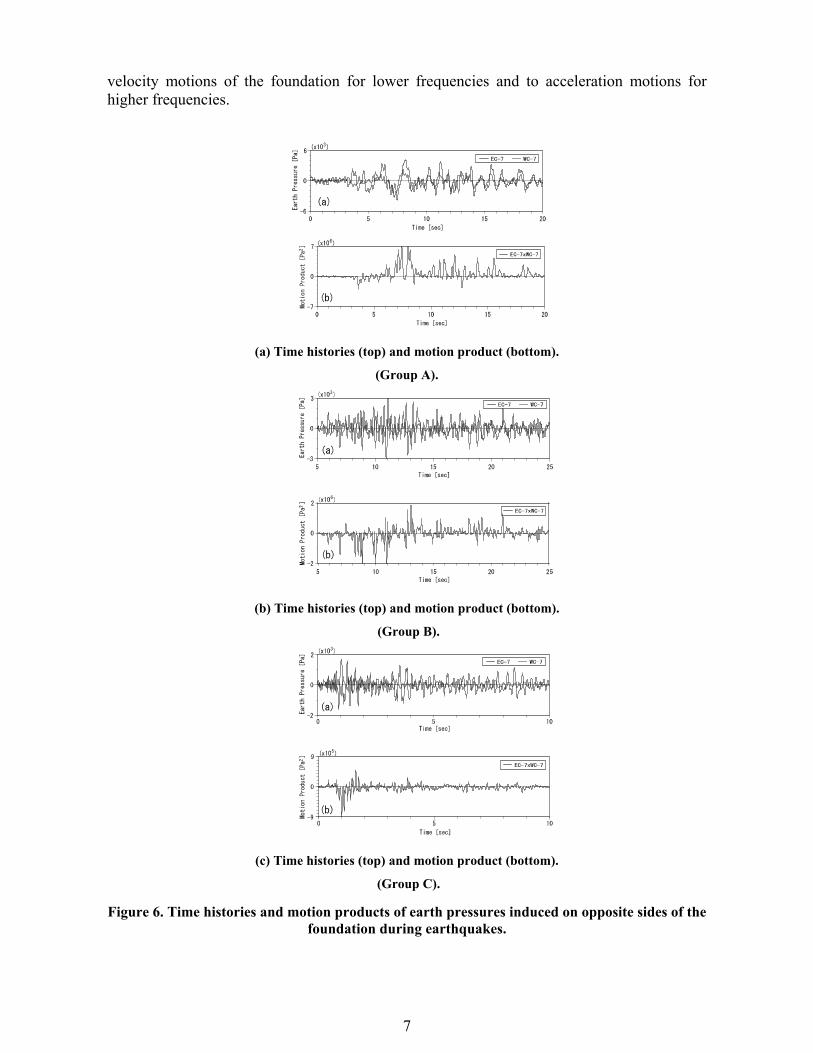
Phase characteristics of earth pressures induced on both sides of the foundation can be extracted by calculating the motion products of the earth pressures recorded on both sides. The computed results of the motion products are shown in figures 6(a), (b) and (c) for the representative motions of each group. The positive value of the product can be interpreted as the earth pressures on both sides being induced in phase on both sides, and the negative values of the product, on the other hand, imply the generation of earth pressures with a phase lag out of 180 degrees on two sides. Inspection of the results shown in figure 6(a) indicates that for the ground motions of group A the earth pressures induced on both sides are almost in phase throughout the record. It should be noticed that the in-phase phenomenon of the earth pressures cannot be explained by the conventional assumption of the vertical incidence of seismic waves.

As for group B shown in figure 6(b), the earth pressures induced on both sides of the foundation are showing out-of phase in the primary portion of the time history and tend to shift to in-phase with progress of time. With regard to the motions of group C, which contains higher frequencies, out-of-phase and in-phase phenomena are recognized alternately throughout the whole time history as shown in figure 6(c). Summarizing the results shown in figures 6(a), (b) and (c), it may be noted that the phase characteristics of earth pressures induced on both sides of the foundation are strongly affected by frequency components contained in the ground motions and tend to be induced in phase for the ground motions with lower frequencies.

Another point to be discussed is what components of foundation motions are closely related to the earth pressures. Observed time histories of earth pressures and velocity response of foundation are shown simultaneously in figures 7(a), (b) and (c) for respective ground motions of groups A, B and C. It will be noticed that the earth pressures are closely correlated with velocity motions of foundation for groups A and B. As for group C, on the other hand, the close correspondence between the two is not recognized as shown in figure 7(c). Figure 8 shows time histories of earth pressures and acceleration motions of the foundation from 0 to 10 sec (top) and 10 to 20 sec (bottom). A strong correlation between the earth pressures and acceleration motions of the foundation for group C is recognized. Finally, figures 9(a) to (e) show Fourier amplitude spectrum ratios of the earth pressures observed at different points to the velocity motions of foundation. The results are smoothed by use of Parzen window with a bandwidth of 0.2 Hz. It will be noticed that the spectrum ratios are almost constant for frequencies less than 4 5∼ Hz and tend to increase almost linearly for higher frequency. This fact indicates that earth pressures are induced in accordance with

Figure 5. Normalized Fourier spectra of ground motions of Group A, B and C.

7

velocity motions of the foundation for lower frequencies and to acceleration motions for higher frequencies.

(a) Time histories (top) and motion product (bottom).

(Group A).

(b) Time histories (top) and motion product (bottom).

(Group B).

(c) Time histories (top) and motion product (bottom).

(Group C).

Figure 6. Time histories and motion products of earth pressures induced on opposite sides of the foundation during earthquakes.

8

Figure 7. Time histories of earth pressures and velocity responses of foundation.

Figure 8. Time histories of earth pressure and acceleration response of foundation (Group C).

Figure 9. Spectrum ratios ofearth pressures to velocityresponse of foundation.

(a) Group A

(b) Group B

(c) Group C

9

ANALYSIS OF LATERAL SOIL RESISTANCE

Description of problem and formulation

The objective of this chapter is to present formulation for analyses of the lateral soil resistance to the foundation when excited by a lateral harmonic force applied on the foundation. The foundation-soil system considered in this study is shown in figure 10. The laterally extending soil is composed of two horizontal layers with hysteretic material damping, which is supposed to be supported rigidly at the base. The soil is assumed to be composed of two-dimensional medium of plane strain with unit width. The coordinate systems x and z are chosen as shown in figure 11.

On the assumption that the vertical displacements in each layer are negligibly small compared to the horizontal component, the equations of harmonic motion for each layer can be written by,

Layer 1； 2 2

21 11 1 1 1 12 2(1 2 ) 0u uih E G u

x zρ ω

∂ ∂+ + + = ∂ ∂

(1)

Layer 2； 2 2

22 22 2 2 2 22 2(1 2 ) 0u uih E G u

x zρ ω

∂ ∂+ + + = ∂ ∂

(2)

where ω =circular frequency of harmonic excitation, lu = horizontal displacement for l -th layer ( 1,2l = ), lρ = mass density of medium, and lh = material damping factor of hysteretic type, and lE = Young’s modulus of soil, which can be expressed with Lame’s constants ,l lG λ as follow.

2l l lE Gλ= + , 1,2l = (3)

Figure 10. Analysis model of foundation-lateral soil system.

Figure 11. Coordinate system and earth pressure induced on the interface between foundation and the lateral soil.

10

Under the condition of absence of vertical displacements, the normal stress in the soil ( , )x x zσ may be expressed with horizontal displacement as follows.

( , ) (1 2 ) lx l l

ux z ih Ex

σ ∂= +

∂ , 1, 2l = (4)

The boundary conditions on the surface, on the intermediate soil interface and at the bottom of soil may be expressed by,

1 2

11 2 ; 0

z H H

duz H Hdz = +

= + = (5-1)

2 1 2 2 2; ( ) ( )z H u H u H= = (5-2)

2 2

1 21 1 2 2(1 2 ) (1 2 )

z H z H

du duih G ih Gdz dz= =

+ = + (5-3)

20 ; (0) 0z u= = (5-4)

where 1H and 2H are the thickness of the first and the second layer, respectively.

In a similar manner, the boundary conditions on the lateral surface of the foundation and the radiation condition at infinity may be expressed by

11 1 2 1 20 ; (1 2 ) ( ),ux ih E p z H z H H

x∂

= + = − ≤ ≤ +∂

(6-1)

22 2 2(1 2 ) ( ), 0uih E p z z H

x∂

+ = − ≤ ≤∂

(6-2)

1 2; 0, 0x u u= ∞ → → (6-3)

where ( )p z is the amplitude of lateral normal stress that the foundation exerts on the lateral surface of the layered soil.

In analyzing of Eqs (1) and (2) under the boundary conditions above, we summarize these two equations as follows for convenience.

2* * 2

2( ) ( ) ( ) 0u d duE z G z z ux dz dz

ρ ω∂ + + = ∂ (7)

where,

1 2 1 2

2 2

( , ) ;( , )

( , ) ;0u x z H z H H

u x zu x z z H

< < += < <

(8)

1 1 2 1 2*

1 2 2

(1 2 ) ;( )

(1 2 ) ;0ih G H z H H

G zih G z H

+ < < += + < <

(9-1)

1 1 2 1 2*

1 2 2

(1 2 ) ;( )

(1 2 ) ;0ih E H z H H

E zih E z H

+ < < += + < <

(9-2)

and,

11

1 2 1 2

2 2

( ) ;( )

( ) ;0z H z H H

zz z H

ρρ

ρ< < +

= < < (9-3)

Employing the method of separation of variables for the displacement ( , )u x z , we write as

1

2

( , )( , ) ( ) ( )

( , )u x z

u x z X x U zu x z

= =

(10)

As for the displacement component along the depth of soil ( )U z , we adopt the fundamental mode shape of the two layering soil. Letting ( )U z be as

1 2 1 2

2 2

( ),( )

( ), 0U z H z H H

U zU z z H

≤ ≤ += ≤ ≤

(11)

the mode shapes for the first and second layers 1 2( ), ( )U z U z may be given by

11 1 2

1

( ) cos ( )s

U z C H H zVω

= + − , 2 1 2H z H H≤ ≤ + (12-1)

11

1 12

1 22

2

cos( ) sin

sin

s

s

s

HVU z C z

VHV

ωω

ω= , 20 z H≤ ≤ (12-2)

where C = integral constant, and 1 2,s sV V are shear wave velocities of soil layers as given by

2 21 21 2

1 2

,s sG GV Vρ ρ

= = (13)

It may be easily shown that these functions satisfy the boundary conditions of Eqs (5). In Eqs (12) 1ω is the fundamental circular frequency of the shear-column of two layering soil without damping, and is given by the minimum root of the following characteristic equation.

2 12 1 2

2 1 2 1 1 2

cos cos sin sin 0s s s s s s

G GH H HV V V V V V

ω ω ω ω− + = (14)

The participation factor of the shear-column when vibrating with the fundamental mode may be given by

{ }

1 2

1 2

01 2

0

( ) ( )

( ) ( )

H H

H H

z U z dz

z U z dz

ρβ

ρ

+

+

⋅= ∫∫

(15)

Next, substitution from Eq. (10) into Eq. (7) gives

2

* * 22( ) ( ) ( ) 0d X d dUE z U X G z z U X

dx dz dzρ ω + + ⋅ =

(16)

Multiplying Eq. (16) by ( )U z and integration with respect to z in the range [ ]1 20, H H+ ,

and multiplying 21β on both sides of the equation, then we will arrive at

12

22

2 0e e en s

d Xk k X m Xdx

ω− + = (17)

This equation of motion is equivalent to that of a system which is composed of an axial rod supported on continuously distributed shear soil spring. The parameters appearing in this equation ,e e

sm k and en k are given by

{ }1 2 221 0

( ) ( )H Hem z U z dzβ ρ

+= ∫ (18-1)

1 22 *1 0

( ) ( )H He

sd dUk G z U z dzdz dz

β+ = −

∫

1 22

2 *1 0

( )H H dUG z dz

dzβ

+ = ∫ (18-2)

{ }1 2 22 *1 0

( ) ( )H He

n k E z U z dzβ+

= ∫ (18-3)

It should be noted that these are complex valued except for em .

Substituting from Eq. (15) into Eqs (18-1) and (18-2), we will obtain other forms for ,e e

sm k as

{ }

{ }

1 2

1 2

2

0

2

0

( ) ( )

( ) ( )

H H

eH H

z U z dzm

z U z dz

ρ

ρ

+

+

⋅=∫∫

(19)

1 2

2*

02

*

0

( )

( )

zes

H H

dUG zdz

kdUG z dzdz

=

+

=

∫

(20)

Equivalent multi-lumped-mass model

Introducing a discretization procedure for Eq. (17) with an equally spaced finite difference approximation, it is possible to rewrite as

( )21 12 0e e e e e

n j n s j n jK X K K M X K Xω− +− + + − − = (21)

where jX is the horizontal displacement of the j-th mass, and other parameters appearing in this equations are defined as

1e en nK k

x=∆

, e es sK x k= ∆ , e eM xm= ∆ (22)

in which x∆ is a mass interval of spacing. We will notice that Eq. (21) is nothing but an equation of motion of a lumped-mass system connected in series as shown in figure 12, and

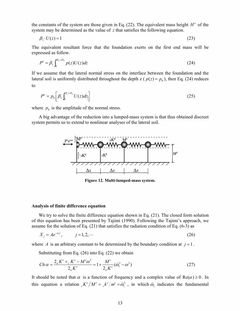
13

the constants of the system are those given in Eq. (22). The equivalent mass height eH of the system may be determined as the value of z that satisfies the following equation.

1 ( ) 1U zβ ⋅ = (23)

The equivalent resultant force that the foundation exerts on the first end mass will be expressed as follow.

1 2

1 0( ) ( )

H HeP p z U z dzβ+

= ∫ (24)

If we assume that the lateral normal stress on the interface between the foundation and the lateral soil is uniformly distributed throughout the depth z ( 0( )p z p= ), then Eq. (24) reduces to

1 2

0 1 0( )

H HeP p U z dzβ+ = ∫ (25)

where 0p is the amplitude of the normal stress.

A big advantage of the reduction into a lumped-mass system is that thus obtained discreet system permits us to extend to nonlinear analyses of the lateral soil.

Figure 12. Multi-lumped-mass system.

Analysis of finite difference equation

We try to solve the finite difference equation shown in Eq. (21). The closed form solution of this equation has been presented by Tajimi (1990). Following the Tajimi’s approach, we assume for the solution of Eq. (21) that satisfies the radiation condition of Eq. (6-3) as

jjX Ae α−= , 1, 2,j = (26)

where A is an arbitrary constant to be determined by the boundary condition at 1j = .

Substituting from Eq. (26) into Eq. (22) we obtain

2

2 21

2 1 ( )2 2

e e e en s

e en n

K K M MChK K

ωα ω ω+ −= = + − (27)

It should be noted that α is a function of frequency and a complex value of Re( ) 0α ≥ . In this equation a relation 2

1e e e e

s sK M k m ω= = , in which 1ω indicates the fundamental

14

circular frequency of the shear-column of the layered soil, is made use of. Though the value α may be determined by solving Eq. (27), the analysis of the transcendental equation is not necessary as seen below.

Next step is to determine the arbitrary constant A in Eq. (26). The constant A may be determined from the boundary conditions for the first mass. Taking into account that the governing region of the end mass is a half of the other masses, the equation of motion for the first mass ( 1j = ) may be given as follows.

21 2

1 12 2

e e e e en s nK K M X K X Pω + − − =

(28)

Substituting from Eq. (26) into Eq. (28), it may be found that A is given by

1 ee

n

eA PSh K

α

α= (29)

Substitution Eq. (29) into Eq. (26) leads to the solution of the finite difference equation as shown by

( 1)e

jj e

n

PX eK Sh

α

α− −= (30)

By setting 1j = in this equation, we will obtain the relationships between the equivalent excitation force eP and the displacement of the first mass as shown by

1e e

nP K Sh Xα= ⋅ (31)

In this equation en K Shα implies the equivalent dynamic stiffness of the lateral layering soil

of a unit width perpendicular to the plane, in which en K is the lateral stiffness of the lumped-

mass system when the second mass kept immovable and Shα represents the effects of the other masses connected laterally. Making use of the relation 2 2 1Ch Shα α− = and from Eq. (27), we will obtain an explicit form for Shα as

2 2 2 21 1

1( ) 1 ( )4

e e

e en n

M MShK K

α ω ω ω ω= − + − (32)

Finally, substituting from Eq. (31) into Eq. (25), the magnitude of earth pressure 0p generated on the side of the foundation may be evaluated by

1 20 1

1 0( )

e

H HK Shp X

U z dz

α

β+=

∫ (33)

It should be noted that 1X in Eq. (33) is equivalent to the amplitude of a horizontal displacement of the foundation at the equivalent height eH , which may be evaluated on the basis of the observations during the forced vibration tests.

15

ANALYSIS OF EARTH PRESSURE DURING EARTHQUAKES

Analysis model and assumptions

The model adopted in this study for the analysis of earth pressures during earthquakes is illustrated in figure 13. It consists of a rigid foundation supported by sway and rocking springs and dashpots which represent radiation damping into subsoil below foundation, and two series of lumped-mass system representing the dynamic resistance of the laterally extending soil. As described earlier the observed results of the earth pressures induced on the opposite sides of the foundation during earthquakes cannot be explained by an assumption of vertical incidence of seismic waves. In the analysis of the soil-foundation system subjected to ground motions, therefore, we assume in this paper an oblique incidence of seismic waves that propagate in the x-direction.

In formulation of response analyses of the system, the whole system is divided into three substructures: two of them are right and left lateral lumped-mass systems as shown in figure 14, and the other is the rigid foundation subjected to the ground motions at the base and horizontal forces from the lateral soil. The input motions into the foundation from the lateral soil are included in the formulation of the lateral lumped-mass systems. The coordinate x is defined as shown in figure 13 with the origin at the center of the foundation base. In the seismic response analysis of the whole system, it will become a key step to evaluate the response of lateral lumped-mass systems when subjected to both the ground motions and horizontal forces exerted from the lateral soil.

Figure 13. Lumped-mass model for response analysis of foundation-lateral soil system.

Figure 14. (a) Lumped-mass system for the lateral soil of the right side, and (b) the left side.

(a)

(b)

16

Earthquake response analyses of system

The response of the lumped-mass system connected in series shown in figure 14 may be expressed by the sum of two responses. One is the response to a harmonic excitation applied at the end mass, which has been given before, and the other is one to the harmonic ground motions. Thus, the total response of the system may be expressed by the sum of two responses as

(1) (2)j j jX X X= + (34)

where the first term of the right side represents the response to the excitation applied at the end mass, and the second to the ground motions. Making use of the result expressed in Eq. (30) the response to the excitation at the end mass of the right side shown in figure 14(b) may be expressed by

(1) ( 1)e

jRj e

n

PX eK Sh

α

α− −= (36)

where eRP indicates the equivalent lateral force generated on the interface between the

foundation and the lateral soil extending to the right direction.

Next step is to analyze the lumped-mass system when subjected to traveling ground motions at the base of each mass. A harmonic seismic waves traveling to x-direction with an apparent wave velocity c on the surface of the supporting bed rock, may be expressed as follows.

( / )0( , ) i t x c

gu x t u e ω −= (37)

where 0u is the amplitude of the harmonic ground motions.

Letting the response of the j th− mass of the system be (2) i tjX e ω , the equation of motion

governing the lumped-mass system may be expressed by

( )(2) 2 (2) (2)1 12e e e e e e

n j n s j n j s g jK X K K M X K X K Uω− +− + + − − = , 2,3,j = (38)

where g jU is the amplitude of ground motion at the j th− mass, which is defined as follows with wave number /k cω= :

0jikx

g jU u e−= (39)

in which jx is horizontal distance from the center of the foundation to the j th− mass, and may be given as,

/ 2 ( 1)jx L x j= + ∆ − (40)

with full length of the foundation L and the spacing of mass x∆ .

For the first mass, the equation of motion may be expressed by

( )2 (2) (2)1 2 12 2e e e e e

n s n s gK K M X K X K Uω+ − − = (41)

The general solution for Eq. (38) will be given as follows.

17

{ }/ 2 ( 1)(2)0( ) ik L x jj

j RX H Ae e uαω − +∆ −− ⋅ = + (42)

where A is an arbitrary constant to be decided so as to satisfy Eq. (41), and is given as

( / 2)sin ikLk xA i eSh

α

α−∆

= − (43)

In Eq. (42), RH is defined as

( )

21

2 21

( )2 1 cos

R en

e

HK k x

M

ωωω ω

=− + − ∆

(44)

where 21ω indicates the fundamental circular frequency of the lateral layering soil and

defined as

21

es

e

KM

ω = (45)

The function RH is interpreted as a frequency response factor of the multi-lumped-mass system when subjected to non-vertical incidence of seismic waves.

Thus, the total harmonic response of the first mass in the right side when subjected to both the horizontal excitation from the foundation and the ground motions, will be obtained by substitution of Eqs (36) and (42) with Eq. (43) into Eq. (34), and it leads to

/ 21 0

sin 1( ) 1ikL eR Re

n

k xX H e i u PSh K Sh

ωα α

− ∆= − +

(46)

In a similar manner, the harmonic response of the first mass in the left side of the foundation 1

i tX e ω− will be finally expressed by

/ 21 0

sin 1( ) 1ikL eL Le

n

k xX H e i u PSh K Sh

ωα α−

∆= + −

(47)

where eLP is an amplitude of the horizontal excitation applied at the first mass in the left side.

The LH in Eq. (47) is the same as RH , which is defined in Eq. (44).

It should be noted here that the responses of the first masses in the right and left sides of the foundation, 1X and 1X − , are equal to the foundation response of the foundation at the level of the equivalent height of the mass system.

Formulation for response analysis of foundation

The final step of the analyses is the analysis of response of the rigid foundation subjected to excitations from the both sides of the foundation and earthquake ground motions at the base. In evaluation of the foundation input motion when subjected to oblique incident seismic waves, an averaging procedure proposed by Iguchi (1973) is adopted. The horizontal component of the foundation input motion * i tU e ω may be evaluated by

18

* 1 ( , )i tgA

U e u x t dAA

ω = ∫ (48)

where A is base area of the foundation. Substitution from Eq. (37) into Eq. (48) and integration over the area leads to

*0

sin( / 2)/ 2

kLU ukL

= (49)

Assuming vertical incidence of incoming waves ( c →∞ or 0k → ) in Eq. (49), the amplitude of the foundation input motion will be equal to that of the incident wave and thus

*0U u= .

The equation of motion for the rigid foundation subjected to both horizontal excitations from the lateral sides of the foundation and the ground motions may be expressed as follows.

02 0 02 2

00

//( ) / /( )

eH G

ee e eR G

K M h M HHK H h M H J H

ω ∆⋅

− Φ⋅

2 *0

1 1 1/ 1 1

eR

e eG L

PM U B

h H Pω

= − −

(50)

where 0∆ and 0Φ are horizontal and rocking motions at the base of the foundation, Gh = the height of the gravity center of the foundation from the base, B = width of the foundation,

eH = equivalent height of mass connected in series, 0M = mass of the foundation, and J = a mass moment of inertia of the foundation with respect to its bottom, which may be evaluated by

20 0GJ J h M= + (51)

with a mass moment of inertia 0J with respect to the gravity center of the foundation.

In Eqs (46) and (47), it should be reminded that 1X and 1X − are equal to the horizontal displacements of the foundation at the equivalent height of the mass system. Thus we hold

*1 1 0 0

eX X H U−= = ∆ + Φ + (52)

Substituting from Eq. (52) into Eqs (46) and (47), we will obtain the expressions for the resultant earth pressures on the lateral sides of the foundation e

RP and eLP .

* / 20 0 0( ) ( ) ( sin )e e e e ikL

R n nP K Sh H U H K e Sh i k x uα ω α−= ∆ + Φ + − − ∆ (53) * / 2

0 0 0( ) ( ) ( sin )e e e e ikLL n nP K Sh H U H K e Sh i k x uα ω α= − ∆ + Φ + + + ∆ (54)

where we set ( ) ( ) ( )R LH H Hω ω ω= = .

Substituting from Eqs. (53) and (54) into Eq. (50), the equation of motion for the foundation may be finally expressed by

02 0 02 2

00

2 2 /2 /( ) 2 / /( )

eH L L G

ee e eL R L G

K K K M h M HHK K H K h M H J H

ω ∆+

− Φ+

19

2 * *0

1 12

/ 1LeG

M U K Uh H

ω

= −

0

1sin / 2sin2 ( ) cos / 21L

kL k xH K kL uSh

ωα

∆+ −

(55)

where HK and RK are the horizontal and rocking springs defined at the base of the foundation, which are the function of frequencies and complex valued. These complex springs represent the soil stiffness evaluated excluding the effects of lateral soil. In addition,

LK in Eq. (55) is a complex spring for the lateral side of the foundation. e

L nK B K Shα= (56)

Once the sway and rocking responses of the foundation are solved from Eq. (55) for given ground motions, the resultant earth pressures on the lateral sides of the foundation can be evaluated from Eqs (53) and (54). The earth pressure in a unit area under the assumption of uniform distribution of the contact stress may be evaluated from Eq. (33).

Theoretical discussion of earth pressure during earthquakes

Based on Eqs (53) and (54) the expressions of the lateral earth pressures on both sides of the foundation under the action of earthquake ground motions may be rewritten as follow.

*0 0 0

sin / 2sin( ) ( ) cos / 2e e e eR n n

kL k xP K Sh H U H K Sh kL uSh

α ω αα

∆= ∆ + Φ + − −

0cos / 2sin( ) sin / 2e

nkL k xiH K Sh kL u

Shω α

α ∆

+ +

(57)

*0 0 0

sin / 2sin( ) ( ) cos / 2e e e eL n n

kL k xP K Sh H U H K Sh kL uSh

α ω αα

∆= − ∆ + Φ + + −

0cos / 2sin( ) sin / 2e

nkL k xiH K Sh kL u

Shω α

α ∆

+ +

(58)

It should be noted here that compressive soil pressures are supposed to be positive. The first terms of the right hand side of Eqs (57) and (58) corresponds to earth pressures induced on the sides of the foundation by the horizontal motion of the foundation when the lateral soils are free from the ground motions. These terms will result in causing out-of-phase earth pressures on the opposite sides of the foundation. The second and the third terms of these equations correspond to the earth pressures induced by ground shaking when solely the lateral soils are subjected to earthquake motions while the foundation is kept immovable. By further inspection of these terms, we will notice that the second terms of Eqs (57) and (58) will cause out-of-phase earth pressures on the opposite sides, and on the other hand the third term the in-phase pressures. This fact indicates that the third terms of Eqs (57) and (58) will cancel each other, and will not be effective as input motions into foundation from the lateral sides of the foundation.

For the case c →∞ or 0k → , which corresponds to the vertical incidence of seismic waves, the third terms of Eqs (57) and (58) will disappear and the phenomenon of in-phase earth pressures will never occur. The earth pressures for the group C, which contains

20

predominantly higher frequencies in the ground motions, have shown a close correlation with the acceleration motion of the foundation response. This tendency may be explained by inspection of Eqs (57) and (58) as follows. If considering the caseω →∞ , we will obtain as

2 , ( ) .e e en nK Sh M H K Sh constα ω ω α→ →

As a result, with increase of ω the first term will be dominant comparing to the other terms. This implies that the first terms of the equations tend to have significant effect on the earth pressures for large value ofω , and to cause the out-of-phase earth pressures on the opposite sides of the foundation. It is obvious that the first terms of Eqs (57) and (58) are proportional to the acceleration response of the foundation.

Finally we will extend the discussion to the case of static earth pressures by considering 0ω → in Eq. (44). For 0ω → , we will obtain ( ) ( ) 1RH Hω ω= → , .e

n K Sh constα → and 0k → . With consideration of these limits, the expressions of the earth pressures on both

sides of the foundations will be given as follows. * *

0 0 0 0 0 0( ), ( )e e e eR LP H U u P H U u∝ ∆ + Φ + − ∝ − ∆ + Φ + −

We will notice that *0 0 0( )eH U u∆ + Φ + − represents the longitudinal strain at the interface

between the foundation and the surrounding soil. On the other hand, the longitudinal particle velocity of soil at the interface is equal to the velocity of the foundation. Thus, reminding the fact that for one dimensional wave propagation of an elastic medium the longitudinal strain is proportional to the particle velocity of the medium (Minowa et al. 2001), the above equations may be rewritten as,

* *0 0 0 0( ), ( )e e e e

R LP H U P H U∝ ∆ + Φ + ∝ − ∆ + Φ +

These expressions indicate that for lower frequencies the earth pressures will be induced in response to the velocity motion of the foundation. This may be paraphrase as the earth pressure will be induced in proportional to the relative horizontal displacement motions between the foundation and the surrounding soil.

It may be summarized that the simplified analysis model presented in this paper can successfully explain the observations of earth pressures during earthquakes.

COMPARISON OF ANALYTICAL RESULTS WITH OBSERVATIONS

- FORCED VIBRATION TEST-

Parameters of lumped mass system

The parameters of the multi-lumped-mass system shown in figures 9 and 13 were determined basically on the basis of the soil constants shown in figure 1. As the damping constants of soil, however, were not measured we were obliged to assume the damping factors of a hysteretic type and we assumed for the first and the second soil layers as

1 2h h h= = and 0.1h = . Additionally, the computed results of the first to the third frequencies of the layered soil evaluated from Eq. (14) were 1 4.4 ,f Hz= 2 9.8 ,f Hz=

3 18.4f Hz= . Thus obtained fundamental frequency 1 4.4f Hz= is larger than 1 3.5f Hz≈ that was expected by observations. The discrepancy between these two may be attributed mainly

21

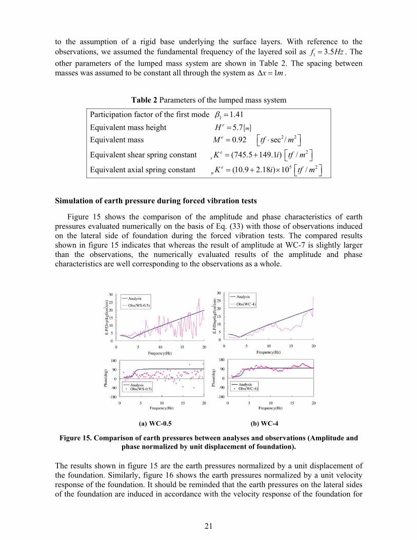
to the assumption of a rigid base underlying the surface layers. With reference to the observations, we assumed the fundamental frequency of the layered soil as 1 3.5f Hz= . The other parameters of the lumped mass system are shown in Table 2. The spacing between masses was assumed to be constant all through the system as 1x m∆ = .

Table 2 Parameters of the lumped mass system

Participation factor of the first mode 1 1.41β = Equivalent mass height eH =5.7 [ ]m Equivalent mass 0.92eM = 2 2sec /tf m ⋅

Equivalent shear spring constant (745.5 149.1 )es K i= + 2/tf m

Equivalent axial spring constant 5(10.9 2.18 ) 10en K i= + × 2/tf m

Simulation of earth pressure during forced vibration tests

Figure 15 shows the comparison of the amplitude and phase characteristics of earth pressures evaluated numerically on the basis of Eq. (33) with those of observations induced on the lateral side of foundation during the forced vibration tests. The compared results shown in figure 15 indicates that whereas the result of amplitude at WC-7 is slightly larger than the observations, the numerically evaluated results of the amplitude and phase characteristics are well corresponding to the observations as a whole.

(a) WC-0.5 (b) WC-4

Figure 15. Comparison of earth pressures between analyses and observations (Amplitude and phase normalized by unit displacement of foundation).

The results shown in figure 15 are the earth pressures normalized by a unit displacement of the foundation. Similarly, figure 16 shows the earth pressures normalized by a unit velocity response of the foundation. It should be reminded that the earth pressures on the lateral sides of the foundation are induced in accordance with the velocity response of the foundation for

22

higher frequencies more than 3 4Hz∼ . This tendency is successfully explained by a simplified multi-lumped-mass model developed in this study.

(a) WC-0.5 (b) WC-4

Figure 16. Comparison of earth pressures between analyses and observations (Amplitude and phase characteristics normalized by unit velocity of foundation).

NUMERICAL ANALYSIS OF EARTH PRESSURE DURING EARTHQUAKES

Evaluation of sway and rocking stiffness

In order to evaluate numerically the earthquake response of the foundation on the basis of Eq. (55), it is required to obtain the sway and rocking stiffness for the foundation motions. In the numerical analyses, these values were determined on the basis of the sway and rocking responses of the foundation observed during the forced vibration tests. Let the horizontal and rocking responses of the foundation be denoted by 0 0,i t i te eω ω∆ Φ for harmonic excitations applied on the foundation i tPe ω as shown in figure 17(a). The sway and rocking stiffness of the soil underlying the foundation, HK and RK , which are shown in figure 17(b), may be evaluated by

20 0 0 0 0

0

1 ( ) 2( )eH g LK P M h H Kω = + ∆ + Φ − ∆ + Φ ∆

(59)

2 2

0 0 0 0 00

1 2( )e eR p g LK Ph M h J H H Kω ω = + ∆ + Φ − ∆ + Φ Φ

(60)

where ph is the height of the applied force ( ph =7.2m), and LK is the lateral soil stiffness for

the foundation, which is defined in Eq. (56). It should be noted that 0 0,∆ Φ in Eqs (59) and (60) are complex valued amplitudes of the foundation. Figures 18(a) and (b) show the results of HK and RK evaluated on the basis of Eq. (59) and (60). Inspection of figure 18 reveals

23

that these values vary strongly with frequencies higher than 7 10Hz∼ , that is probably due to the effect of deformation of the foundation base.

Ground motions at the foundation base

As mentioned in the earlier section, the phase characteristics of earth pressures being induced in-phase on both sides of the foundation cannot be explained by an assumption of the vertical incidence of seismic waves. The same phenomenon was observed in observations using a small model foundation (Uchiyama et al. 1999). Uchiyama et al. (1999) tried to explain the phenomenon by using FEM and assuming a non-vertical incidence of seismic waves. Following Uchiyama et al. (1999) we assume here oblique incidence of waves. Consequently, in evaluation of the foundation responses and earth pressures during earthquakes, it is required to determine the apparent wave velocity c traveling horizontally in the soil at the level of the foundation base, as well as the time history of the ground motions at that depth.

As for the apparent wave velocity c, the value would depend mainly on shear wave velocity of the supporting soil and on the azimuth and incident angle of seismic waves, among which the latter two cannot be decided from the observed data. A parametric study, therefore, was conducted with respect to c by changing the value in the range

3,000 100,000 / secc m= ∼ . By inspection of the results of the parametric studies, 10,000 / secc m= was chosen as the appropriate value regardless of the earthquake motions.

(a) Foundation Response to Excitation. (b) Resistant Model of Foundation to Excitation.

Figure 17. Forced excitation test and equivalent resistance model of foundation.

(a) Sway Spring. (b) Rocking Spring.

Figure 18. Complex stiffness at the base of foundation.

24

On the other hand, as for the time histories of the ground motions at the level of the foundation base, which is supported at –8.2m from the soil surface, the ground motions at the depth have not been observed directly. Therefore, the ground motions at the level were evaluated numerically by means of the Thomson-Haskel’s method and with use of the ground motions recorded in the free field at the depths of –1m and –40m. The details of the evaluation of the ground motions at this site may be found elsewhere (Iguchi et al. 2000) and will not be repeated here.

Comparison of velocity response of foundation

The velocity responses of the foundation evaluated numerically on the basis of Eq. (55) are compared with observations. Figures 19(a), (b) and (c) show the compared results in terms of Fourier amplitudes between the two. As seen from the figures, fairly good agreement between two are obtained for groups A and B up to 10 Hz, whereas slight discrepancies may be recognized for group C. It was confirmed that the simplified analysis model proposed in this paper gives satisfactory results and may be applicable to numerical simulation analyses of the embedded foundation directly supported on a firm soil.

Comparison of time histories of earth pressures

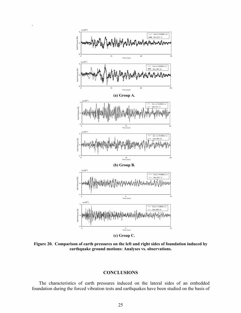
Figures 20(a), (b) and (c) show the compared results of numerically evaluated time histories of the earth pressures induced on both sides of the foundation with those of observations for groups A, B and C. In the calculations, the apparent wave velocity c was assumed to be 10,000m/s. As seen from figure 20, whereas somewhat discrepancy was recognized for group C, fairly good agreement between the numerically evaluated results and observations were detected for groups A and B. One of the main reasons of the discrepancy might be attributed to uncertainties inherent to ground motions with high frequencies. It was confirmed that the multi-lumped-mass model presented in this paper is applicable not only for response analyses of a foundation but for the numerical simulation of the earth pressures induced by earthquake ground motions.

(a) Group A. (b) Group B. (c) Group C.

Figure 19. Comparison of velocity response of foundation: Analyses vs. observations.

25

.

(a) Group A.

(b) Group B.

(c) Group C.

Figure 20. Comparison of earth pressures on the left and right sides of foundation induced by earthquake ground motions: Analyses vs. observations.

CONCLUSIONS

The characteristics of earth pressures induced on the lateral sides of an embedded foundation during the forced vibration tests and earthquakes have been studied on the basis of

26

observations. In addition, a simplified analysis model, which is composed of a lumped-mass system connected in series, was presented to conduct simulation analyses of the earth pressures. The studies have led us following conclusions

(1) The earth pressures during the forced vibration tests tend to be induced associated with the displacement motion of the foundation for frequencies lower than the fundamental frequency of the lateral soil. For frequencies higher than the fundamental frequencies of the soil, one the other hand, the earth pressures tend to be caused in-phase to the velocity motion of the foundation.

(2) The characteristics of earth pressures induced by earthquake motions are strongly dependent on frequency component included in the ground motions.

(3) The earth pressures during earthquakes are strongly related to the horizontal velocities of the foundation for rather lower frequencies and to acceleration response for higher frequencies.

(4) A phenomenon of earth pressures being induced in-phase on opposite sides of the foundation was observed for lower frequencies included in the ground motions. For higher frequencies, on the other hand, the earth pressures tend to be induced out-of-phase on the opposite sides of the foundation.

(5) A simplified analysis model presented in this paper has been proved to be effective in explanation of the observations of earth pressures induced by forced vibration tests.

(6) The analysis model could simulate satisfactorily the observations of earth pressures induced by earthquake motions except for ground motions including higher frequencies.

(7) The phenomenon of earth pressures being induced in-phase during earthquakes could be explained with use of the analysis model and by assuming oblique incidence of seismic waves.

(8) The tendencies of earth pressures on the sides of an embedded foundation being induced in close correlation with acceleration or displacement motions of a foundation could be explained theoretically with use of the simplified analysis model presented in this paper.

ACKNOWLEDGEMENT

This paper is the revision of previously published papers (Iguchi et al. 2001, Iguchi et al.

2002) and we express our gratitude to the coworkers of the papers, Ms. A. Sadohira and Mr.

T. Mutoh.

REFERENCES

Iguchi, M., 1973. Seismic response with consideration of both phase difference of ground motion and

soil-structure interaction, Proc Japan Earthquake Engineering Symposium, 211-218.

Iguchi, M., Unami, M., Yasui, Y., and Minowa, C., 2000. A note on effective input motions based on

earthquake observations recorded on a large shaking table foundation and the surrounding soil (in

Japanese), J. Struct. Constr. Eng., AIJ, No. 537, 61-68.

27

Iguchi, M., Yasui, Y., and Minowa, C., 2001, On Effective Input Motions: Observations and

Simulation Analyses, Proc. of the Second U.S.-Japan Workshop on Soil-Structure Interaction,

Building Research Institute, Ministry of Land, Infrastructure and Transport of Japan, pp75-87.

Iguchi, M., Sadohira, A., and Minowa, C., 2001. Observation and analysis of dynamic earth pressure

on the sides of a large-scale shaking-table foundation during excitation tests (in Japanese), J.

Struct. Constr. Eng., AIJ, No. 549, 75-82.

Iguchi, M., Mutoh, T., and Minowa, C., 2002. Observation and analysis of seismic earth pressures on

the sides of a large-shaking table foundation (in Japanese), J. Struct. Constr. Eng., AIJ, No. 561,

65-72.

Kazama, M., and Inatomi, T., 1988. A study on seismic stability of large scale embedded rigid

structures, Proc. 9th World Conf. on Earthquake Engineering (Tokyo-Kyoto), Vol. Ⅲ , Ⅲ -629 to

Ⅲ -634.

Matsumoto, H., Ariizumi, K., Kuniyoshi, H., Chiba, O., and Watakabe, M., 1990. Earthquake

observation of deeply embedded building structure, Proc. 8th Japan Earthquake Engineering

Symposium, 1035-1040.

Minowa, C., Ohyagi, N., Ogawa, N., and Ohtani, K., 1991. Response data of large shaking table

foundation during improvement works (in Japanese), Tech. Note of the Notional Research

Institute for Earth Science and Disaster Prevention, Report No. 151.

Minowa, C., Iguchi, M., and Iiba, M., 2001. Measurement of lateral earth pressures on an embedded

foundation during earthquakes, Strong Motion Instrumentation for Civil Engineering Structures,

ed. by M. Erdik et al., Kluwer Academic Publishers, 519-532.

Onimaru, S., Sugawara, R., Uetake, T., Sugimoto, M., and Ohmiya, Y., 1994. Dynamic characteristics

of earth pressure on seismic array observation (in Japanese), Proc. 9th Japan Earthquake

Engineering Symposium, 1051-1056.

Ostadan, F., and White, W. H., 1998. Lateral seismic soil pressure: An updated approach, Proc. UJNR

Workshop on Soil-Structure Interaction, Menlo Park, California, 2-1 to 2-36.

Sakai, S., Masuda, A., Imamura, A., Kishino, Y., Ishii, T., Yotsuda, H., and Inoue, T., 1996. Dynamic

earth pressure of deeply embedded building structure, Part 3 Study on dynamic lateral pressure on

basement wall (in Japanese), Summaries of Technical Papers of Annual Meeting, AIJ, 417-418.

Scott, R. F., 1973. Earthquake –induced pressures on retaining walls, Proc. 5th World Conf. Earthq.

Engng, Rome, Italy, Vol. Ⅱ , 1611-1620.

Tajimi, H., 1990. Earth pressures on basement walls induced by soil amplification effects, Proc. 8th

Japan Earthquake Engineering Symposium, 1203-1208.

28

Uchiyama, S., and Yamashita, T., 1999. Experimental and analytical studies of lateral seismic earth

pressure on a deeply embedded building model (in Japanese), J. Struct. Constr. Eng., AIJ, No.

516, 105-112.

Veletsos, A. S., and Younan, A. H., 1994a. Dynamic soil pressures on rigid vertical walls, Earthq.

Engng Struct. Dyn., Vol. 23, 275-301.

Veletsos, A. S., and Younan, A. H., 1994b. Dynamic modeling and response of soil-wall systems, J.

of Geotechnical Engineering, ASCE, Vol. 120, No. 12, 2155-2179.

observations versus analyses: lateral earth … versus analyses: lateral earth pressures on an...

Documents