Observational Learningand Intelligence∗

Alexander Vostroknutov†‡ Luca Polonio Giorgio Coricelli§

July 2016

Abstract

We study experimentally how individuals learn from observing the choices of others in a non-stationary stochastic environment. The imitation choices of participants with low score in anintelligence test are driven solely by the value of imitation. High intelligence score partici-pants, in addition, use choices of others to better understand the environment. They imitatemore when other’s choices are stable, which makes them more optimal than low score partic-ipants. The knowledge that the observed other has high intelligence score affects behavior ofonly low score participants. Overall, intelligence predicts the usage of simple or sophisticatedobservational learning strategy.

JEL classifications: C91, C92Keywords: observational learning, intelligence, bandit problems

∗We would like to thank the participants of the Workshop on “Limited Cognitive Resources in Economics:heuristics, information processing, and strategic behavior,” in Rome as well as Tobias Larsen, Nadege Bault, ErikKimbrough and Andrew Cassey for insightful comments. The authors gratefully acknowledge the financial supportof the European Research Council (ERC Consolidation Grant 617629).†All authors: Center for Mind/Brain Sciences, University of Trento, Via delle Regole 101, 38123 Mattarello (TN),

Italy‡Corresponding author: a.vostroknutov@unitn.it§Department of Economics, University of Southern California.

1 Introduction

Learning is an important and flexible process that allows humans to adapt to their environment.A first basic source of learning comes from personal experience. Humans interact directly withthe environment and learn from the feedback they receive. A second source of learning comesfrom observing other people interacting with the same environment. In a world where we needto adapt quickly to the ever-changing circumstances (e.g., climate fluctuations, socio-politicalcommotion), the ability to learn from others is fundamental because it reduces the effort of ac-quiring information. This is especially true when observational learning is based on simplereinforcement learning mechanisms, which is the case when an agent imitates others, evalu-ates the feedback she receives from the environment and chooses whether to keep imitating ornot depending on the outcome. However, learning from others can be much more than a mereimitation of the observed behavior. A sophisticated way to learn from others includes the under-standing of the rationale behind the observed choices. An agent integrates what she has observedwith the feedback she has directly received from the environment and changes her behavior ac-cordingly. This sophisticated observational learning process is particularly relevant when theenvironment changes and simple imitation becomes not reliable. This sort of learning can bevery efficient but it is also more costly because it requires a higher level of attention and an abil-ity to integrate information from diverse sources. In this respect, intelligence plays an importantrole as it makes it easier for the agent to gather and analyze information.

In this respect, intelligence may be associated with the ability of the agent to acquire andanalyze information.

In this paper we study experimentally the mechanisms of how people learn from others. Inparticular, we are interested in what features of others’ behavior influence imitation and how thisaffects the performance in an uncertain environment. Moreover, we test hypotheses regardingthe role of intelligence and look at the interactions between a measure of intelligence of ourparticipants and the intelligence of the people they observe and learn from.

The knowledge of the interplay of observational learning and intelligence can be very im-portant for policy and issues of economic efficiency. In any environment where people workand/or learn together in fixed groups (school classes, firms etc.) the problems or biases mightarise in who learns what and from whom (given observed levels of intelligence). For example,Braaksma et al. (2002) study the increase in performance in a writing task among 8th graders as

1

dependent on the intelligence of the observed person. They find significant effects of the levelof intelligence of the observed person on the success of the observer, which also depends on theobserver’s intelligence. This raises interesting questions regarding, for example, the division ofpupils into classes according to measures of intelligence.

To study observational learning in a changing environment we look at a two-armed banditproblem with independent non-stationary stochastic processes that determine the payoffs fromthe two arms. In our design, the performance depends on the ability of the participants tochoose the action which gives a reward with higher probability. This is not trivial since theprobability of getting a reward, associated with each action, changes over time. To understandhow participants learn from others, we give them the possibility to observe the choices made byanother person who previously interacted with the same environment, but not outcomes. We donot show the outcomes that the other obtained for two reasons: 1) observing outcomes wouldreduce the other to just additional information about the environment and 2) the optimality ofthe other would become evident. In addition, participants may or may not receive informationabout the intelligence of the observed person. In this way, we are able to evaluate the effect ofinformation about intelligence on the level of imitation.

Our interest is the exact mechanism of the learning process and the way it is modulatedby the knowledge about owns intelligence and the intelligence of the person observed. Non-stationary environment allows us to distinguish between agents who simply imitate observedbehavior (simple imitation) and agents who use it to better understand the current state of theenvironment (sophisticated imitation). In non-stationary environment agents never stop learning,which makes it possible to study how they adapt throughout the experiment. Conversely, instationary environment it is hard to disentangle imitation of observations of others and ownlearning curves of the observer and the observed.

When addressing the possible influences of intelligence on the mechanisms of how peoplelearn from others, we decided to use a measure of fluid intelligence. In particular we wereinterested in non-verbal abilities and reasoning skills because our learning task is not in anyparticular verbal domain (spelling, reading, comprehension, etc.). Therefore, we used the RavenAdvanced Progressive Matrices (RAPM), a measure of efficient problem solving and abstractreasoning which consists of a series of pattern matching tasks that do not require mathematicalor verbal reasoning abilities (Raven et al., 1998). The performance in Raven test is linked tothe ability to integrate information in sophisticated way. We also collect data about cognitivereflection, the ability to resist an immediate, intuitive and incorrect answer, executed with littledeliberation, in favor of the search for the correct answer requiring a more complex reasoning(Cognitive Reflection Test, proposed by Frederick (2005)). The cognitive abilities measured bythese tests are particularly relevant for the situations faced by participants in this experiment, asin our learning task participants can learn from the information about the observed action usingsimple and/or sophisticated strategies.

2

Our results can be summarized as follows. We do find both simple and sophisticated imitationeffects in our participants. We find that participants with high Raven score use both simpleand sophisticated learning strategies and participants with low Raven scores use only simpleimitation. The imitation of the observed participant is increased when choosing the same actionas the observed participant leads to an increase in earnings (simple imitation). We call thiseffect simple, because it naturally falls into the domain of a rather mechanical reinforcementlearning paradigm where the values of actions are reinforced if they brought higher payoff inthe past. In sophisticated imitation, participants track how stable the choices of the other are,make inferences about what payoffs the observed participant might have received, given herbehavior, and imitate if they infer that the other is getting high payoffs. In addition, we find thathigh Raven participants choose how much attention to pay to the other depending on her ownearnings in the past: the less they earn, the more imitation we observe.

We find an effect of information about the intelligence of the observed participant on the imi-tation strategy. When this information is not available, high Raven participants use both simpleand sophisticated imitation strategies, whereas low Raven participants use only simple imita-tion. In case information is provided both high and low Raven participants use only simpleimitation. This suggests that information about the intelligence of the observed participant isused as a signal of the ability to perform in the task.

We also study how imitation and intelligence of both the observer and the observed influencethe optimality of the choices and the earnings. We find that participants with high Raven scoreschoose more optimally and earn more money than participants with low Raven scores. Only lowRaven participants are affected by the information about Raven score of the observed. In partic-ular, when knowing that the other has high Raven score, they increase imitation which leads tobetter performance. Interestingly, high Raven participants are not affected by this information.These observations suggest that participants with different intelligence levels use different ob-servational learning strategies, which is particularly important considering the large number ofsocial and economic contexts in which people can learn from others.

Finally, we find overall consistency of our data and the imitation choices. In particular, wefind that higher Raven score implies less switching, which, in its turn, leads to higher optimalityand higher earnings. On the behavioral side, we find that high Raven participants imitate more,the less switches they observe, thus learning to perform more optimally in the task. So, highRaven participants are able to correctly interpret what they observe, to learn from it and, thus,better performance, regardless whether the information about the Raven score of the other wasprovided or not. Conversely, low Raven participants need to know the information about theintelligence of the other in order to improve their performance.

3

2 Literature Overview

To our knowledge, we are the first in economic literature to study the mechanisms of observa-tional learning in non-stationary environments. In previous studies this topic was addressedonly in stationary situations and without taking into account the information about the intel-ligence of the observers and observed participants. The literature closest to our study is thatof information cascades (Banerjee, 1992; Bikhchandani et al., 1992; Smith and Sørensen, 2000).In these studies, agents try to learn the qualities of objects from observing the choices of otheragents who are known to have imperfect signals about the qualities of these objects. Unlike thisliterature though, we consider the learning process from one other person, which is a distinguish-ing feature of our study. Observing and learning from the choices of one individual instead ofsequence of single choices by many people can have important features overlooked by the infor-mation cascades literature. In particular, the characteristics of the choices of the observed othercan have an effect on the learning process.

In addition to the information cascades literature there are other examples of observationallearning studies that deserve mentioning. Armantier (2004) shows that observing the opponents’private signals, bids and payoffs in a repeated common value auction homogenizes behavior andaccelerates learning towards Nash equilibrium. Celen and Kariv (2004) show that in a game withpure information externalities over time private information is ignored and decision makersbecome increasingly likely to imitate their predecessors. Merlo and Schotter (2003) show thatin a complete information maximization problem participants can learn better by not doing butwatching someone else’s behavior.

In neuroeconomic literature the most similar study is Burke et al. (2010). The authors userelated learning task (though with stationary environment) and find the correlation of other’saction prediction error and brain activity in dorsolateral prefrontal cortex. The authors claim thatobservational learning is incorporated in standard payoff based learning and demonstrate thiswith a simple reinforcement learning model. The main difference between our approach andthat of Burke et al. (2010) is that in their model observing other choosing an action automati-cally increases the probability of choosing that action. We show that this is not always the caseand that it depends on the past payoffs and past behavior of the observed participant. Anotherrelated study is Nicolle et al. (2011). Here the authors show that people tend to be overly opti-mistic about rewards that they observe being received by someone else (rather than choosing forthemselves). In this study, the payoffs of the observed participant where shown to participants,which makes it rather different from our study and the questions asked.

Some studies consider the connection between cognitive ability and performance in strategicenvironments. Gill and Prowse (2015) look at beauty contest games and find that high Ravenscore is associated with choosing actions closer to Nash equilibrium, with ability to convergefaster to the equilibrium and to earn more than the low Raven score participants. Proto et al.

4

(2014) study the performance in the repeated Prisoner’s Dilemma. They find that, when partic-ipants are grouped into high Raven and low Raven score groups, the high Raven score groupsare able to sustain cooperation, whereas low Raven groups cannot. High Raven groups earnmore than low Raven groups.1 Even though our task does not involve games, the findings inboth studies are in line with what we find: high Raven individuals perform better and earn moremoney.

3 Experimental Design

The study consisted of two experiments: a first experiment in which participants made choicesin 2-armed bandit problem without observing actions of others, and a second experiment inwhich participants made choices in the same environment with only difference that in a half ofthe trials they observed the choices made by one of the two participants selected from the firstexperiment. The purpose of the first experiment was to select two participants, one with highand one with low RAPM score, in order to use them as observed participants in Experiment 2.

The two observed participants were chosen using the following procedure. First, we dividedthe participants into deciles of Raven score. Then we calculated the median number of switchesbetween actions for participants in the first and tenth decile. We chose two participants (one inthe first and one in the tenth decile) who were closest to the median. The aim of this procedurewas to select two participants who would have a prototypical behavior in terms of the numberof switches in the two extremes of the RAPM dimension. We decided to use the number ofswitches parameter for two reasons: 1) it is an index related to the earnings of the participantsand 2) we hypothesized that this is an important parameter that differentiates sophisticated andsimple learners.2,3

Participants in Experiment 2 were divided into four treatments with 2×2 design. The dimen-sions were: 1) the RAPM score of the observed participant (HighRaven or LowRaven) and 2)the information the participants received about the RAPM score of the observed other (Visibleand Not-Visible). The Raven score of the observed participant could be high (28) or low (15).Only participants in the Vis-HighRaven and Vis-LowRaven treatments received this informa-tion. Participants in Novis-HighRaven and Novis-LowRaven treatments were matched with thecorresponding observed participant without knowing his/her score on the RAPM test.

For the main experiment (Experiment 2), 4 Novis and 6 Vis sessions were conducted. Ineach session half of the participants were in the HighRaven condition and the other half in the

1Among other studies on the connection between cognitive ability and strategic reasoning are Benito-Ostolazaet al. (2016); Fehr and Huck (2015); Hanaki et al. (2015); Kiss et al. (2016). An excellent review of broader literature isRustichini (2015).

2Switchiness reflects the need to explore alternative actions when previous outcomes were bad. Ihssen et al.(2016) show that the high number of switches is a sign of high sensitivity to bad outcomes.

3The number of switches of the low and high Raven participants are equal to 49 and 20, respectively.

5

LowRaven condition. All participants were recruited from the subject pool of the Cognitive andExperimental Economics Laboratory at the University of Trento (CEEL). The dates of the sessionsand the number of participants per session are reported in Table 10, Appendix F.

On average participants earned aboute 20.06, in addition to thee 3 show-up fee. The presen-tation of the 2-armed bandit task was performed using a custom made program implementedin Matlab Psychophysical toolbox. The tests and questionnaires were administered with z-Treesoftware package (Fischbacher, 2007). A detailed timeline of the experiment and all instructionsare reported in Appendix C.

3.1 Experiment 1

51 participants took part in Experiment 1. In the first part of the experiment participants madechoices in a 2-armed bandit problem. In the second part they completed a RAPM test of 30 tables,the Holt & Laury Risk Aversion test, the Cognitive Reflection Test and the Empathy Quotientquestionnaire (Baron-Cohen and Wheelwright, 2004).4

After entering the lab, participants were randomly assigned to a PC terminal and were givena copy of the instructions (see Appendix C). Instructions were read aloud by the experimenter,and then a set of control questions were provided to ensure the understanding of the 2-armedbandit problem.

The probabilities of getting a 10 cents reward from each of the two hands followed indepen-dent non-stationary stochastic processes. Figure 1 illustrates.5

0.2

.4.6

.81

0 50 100 150 200

Trials

Probability

Figure 1: The actual probabilities of winning from two options in 200 trials.

Participants were not aware of how the probabilities change but it was made clear that theywould change slowly and independently of their choices, earnings and each other. The 2-armedbandit task included 200 trials divided into four blocks of approximately 50 trials each. At theend of the task participants were not informed about their earnings until after they completed

4The Empathy Quotient questionnaire was developed to assess emphatic abilities in adults with autism-spectrum disorders. This questionnaire was added to the study to assess whether emphatic abilities affect theway participants imitate others.

5The process is a decaying Gaussian random walk with parameters λ = 0.8, decay centre θ = 0.5 and Gaussiannoise with standard deviation 0.2 (see Wunderlich et al. (2009) page 17203 for the exact formula).

6

the second part of the experiment.6 In the second part of the experiment participants were given20 minutes to solve 30 RAPM problems. They were told that they have 20 minutes to solveas many problems as they can and that they would earn 30 cents for each correct answer. Ifparticipants did not complete an item or their answer was incorrect they would earn 0 cents forthat item. At the end of the RAPM test participants completed the Holt and Laury lottery task(with real incentives, see Appendix D), the CRT test and the EQ questionnaire (Appendices Cand E). There was no time limit to complete these three tasks and no payment was provided forthe CRT test and the EQ questionnaire. At the end of the Holt & Laury task a single lottery wasselected at random and played by the computer.

At the end of the second phase, participants were paid according to their choices in the 2-armed bandit problem, their performance in the RAPM problems, the outcome of the selectedlottery and a show-up fee of e 3.

3.2 Experiment 2

In Experiment 2, 160 participants first completed the RAPM test, the Holt & Laury Risk Aversiontest, the Cognitive Reflection Test and the Empathy Quotient questionnaire and then playedin the 2-armed bandit task. The only difference with Experiment 1 (apart from the order ofthe tasks) was that participants in the 2-armed bandit problem, sometimes, and before makingtheir choices, also observed the choices (but not the outcomes) made by one of the two selectedparticipants from Experiment 1. The choices of the observed participant were provided in half ofthe trials (in 100 out of the 200 trials) between trial 10 and trial 200 in blocks of randomized lengthof 5 to 15 consecutive trials. It was made clear to the participants that the observed behaviorwas from a real person who took part in the experiment approximately one month before andthat he/she chose in the same exact environment. Participants knew that the observed otherhas completed all the parts of the experiment, including the questionnaire on matrices problemsthat they completed at the beginning of the experiment. Participants also were informed that theobserved other did not himself observe anyone while completing the 2-armed bandit problemtask.

Participants were shown (and explained) a histogram of the number of RAPM problemssolved by the 51 participants from Experiment 1 (see Figure 9 version a in Appendix C). Inthis way they had the possibility to compare their performance in the RAPM test, which theyknew before starting 2-armed bandit task, with that of the group from which the person theyare going to observe was chosen. The participants were only told that they will receive thisinformation. No information about a possible connection between performances in Raven testand the learning task was provided.

6Participants were not told their total earnings at the end of the learning task, though, in principle, they couldhave calculated it by observing the outcomes after each trial.

7

The instructions were identical for all participants, except for the information that was givenabout the score obtained by the observed participant. In the Novis treatments (Novis-HighRavenand Novis-LowRaven) the score obtained by the observed participant remained unknown (onlydistribution of all Raven score was known). Conversely, in the Vis treatments (Vis-HighRavenand Vis-LowRaven) the score of the observed participant was marked in red on the histogramand also shown on the screen during the experiment (see Figures 9 versions b and c in AppendixC).

Participants were students from the University of Trento, Italy (mean age 23.17, SD 0.23). Thestudy was approved by the local ethics committee and all participants gave informed consent.

4 Results

4.1 Summary Statistics

Before presenting our regression results we start with reporting the summary statistics for Ex-periment 1 and Experiment 2. Table 1 reports the scores obtained in the tests we conducted(average and standard deviation) and demographic information.

Raven CRT HL EQ Gender Age Years studyExperiment 1 21.51 1.46 5.82 40.65 0.57 22.81 2.92

(0.52) (0.19) (0.33) (1.67) (0.08) (0.43) (0.28)

Experiment 2 20.93 1.32 6.02 41.83 0.52 23.17 3.37(0.35) (0.09) (0.13) (0.66) (0.04) (0.23) (0.16)

Table 1: Summary statistics for all data. Earnings reported are for the bandit task only.

A Kolmogorov-Smirnov test was used to test the hypothesis that the distributions of Raven,CRT, HL and EQ scores are different between the two experiments. None of the comparisonswas found to be statistically significant, thus supporting the hypothesis that participants in thetwo experiments come from the same population. This is important because participants inExperiment 2 were presented the distribution of Raven scores of participants from Experiment1 and the absence of significant differences means that they could compare their score with thatof the observed participant in a reliable way.

4.2 Imitation

In this section we present results concerning factors that affect the degree of imitation of theobserved participant. We define the variable im, which equals to 1 if the participant chose thesame action as the observed participant and 0 if she chose a different action.7 First, we want to

7See Appendix A for a description of the variables used in the analyses.

8

look at the aggregate average levels of imitation in the four treatments (Novis-HighRaven, Vis-HighRaven, Novis-LowRaven and Vis-LowRaven) for participants having high vs. low Ravenscores. However, there is a slight complication: there are two reasons why one would choosethe same action as the other. The first is pure imitation (the one we are interested in): the par-ticipant observes what the observed participant has chosen and imitates her. The second is thatthe participant and the other have the same preference-related behavior (the one we want to con-trol): the participant chooses the same action as the observed participant because she thinks thisis the best thing to do regardless of what the observed participant does. To disentangle thesetwo effects we construct a new variable adjim which, for each participant, is equal to the av-erage rate of imitation in periods when the other is observed minus the average rate of samechoice when the other is not observed. The reasoning behind this construction is the following:when a participant chooses on his own without observing the other (in 100 over 200 trials), di-rect imitation is not possible and the choice of the same action is the consequence of the samepreference-related behavior. For each participant, we estimate the average preference-relatedbehavior over 100 periods, when the other is not observed. Given large number of periods, thismeasure should be a good estimate of the preference-related behavior during the periods whenother is observed. Thus subtracting this average imitation rate from the actual imitation duringthe periods of observation should give us a good measure of pure imitation.8

-.05

.05

.15

.25

q1 novis q2 novis q3 novis q1 vis q2 vis q3 vis

High Raven other Low Raven other

+/- 1SE q# - terciles of Raven scores

Adj

uste

d r

ate

of im

itatio

n

Figure 2: The adjusted rate of imitation in Vis and Novis treatments by the terciles of the Ravenscore (q1 - the lowest Raven score; q3 - the highest). Blue (red) bars represent the adjusted rateof imitation in treatments in which participants observed the high (low) Raven other. Spikes are±1 SE.

Figure 2 shows the adjusted average rate of imitation in Novis-HighRaven, Vis-HighRaven,

8One might think that 0.5 is a good estimate of the average imitation rate in periods when the other is notobserved. This would be the case if both participant and the other chose randomly. However, since both are in thesame environment and both try to maximize their earnings the average imitation rate should be strictly above 0.5.Indeed, the average imitation rate when the other is not observed is 0.63.

9

Novis-LowRaven and Vis-LowRaven treatments divided by the Raven score of the participants.9

To shed some light on how different information affects the imitation rate of high and lowRaven participants, we run a regression reported in Table 7 in Appendix B. The dependentvariable is the adjusted rate of imitation (adjim). Independent variables are indicators for treat-ments, terciles of Raven score and all interactions.10 The results support the following obser-vations: high Raven observed participant is imitated more in both Vis and Novis treatments.It means that participants in Novis treatments imitate high Raven other more than low Ravenother even though they do not know the Raven score of the observed participant. Regressionanalysis shows that for the third tercile (high Raven score participants, Novis treatments) the dif-ference in imitation rate is significantly higher than in first tercile (low Raven participants; sumof coefficients obshigh + obshigh×ravterc3, 0.162, p = 0.004).11 This illustrates that high Ravenparticipants in Novis treatments imitate high Raven other more than low Raven participants do.

When participants with low Raven score (first tercile) observe the action of a low Raven ob-served participant without knowing her Raven score (Novis-LowRaven) they tend to imitateher (first red bar from the left). By contrast, when they observe the action of a low Raven ob-served participant knowing her Raven score (Vis-LowRaven) they dismitate her. This difference issignificant (–0.82, p = 0.032).12 Similarly, when participants with low Raven score observe theaction of a high Raven in Vis treatment, they imitate her significantly more (0.0975, p = 0.032)comparing to Novis-HighRaven treatment.13

Conversely, participants with high Raven score (third tercile) do not significantly changetheir rate of imitation upon observing high or low Raven observed participant in Vis and Novistreatments (0.0465, p = 0.406 for low other; –0.0314, p = 0.419 for high other). However, theystill imitate the high Raven observed participant significantly more in both Novis (0.162, p =

0.004) and Vis treatments (0.084, p = 0.033).14

To summarize, participants with low Raven score do strongly react to the information aboutthe Raven score of the observed participant provided to them: the imitation rate drops signifi-cantly when they know that the observed participant has low Raven score and increases signifi-cantly when they know that the Raven score of the observed participant is high. On the contrary,participants with high Raven score do not seem to react much to the information about the Ravenscore of the other. This suggests that low and high Raven score participants use different mecha-

9These results, by construction, represent the actual imitation rate in the four treatments. The interpretations ofthis figure do not change if we consider the not adjusted rate of imitation. See Figure 6 in Appendix B.

10In order to better illustrate the link between reasoning ability and imitation we divide our pool of participantsinto terciles of Raven score. In the future analyses, for the sake of simplicity, we divide participants into below andabove median Raven score.

11The definitions of all variables used in the analyses can be found in Appendix A.12The difference between the two treatments is represented by the coefficient on vis in OLS regression in Table 7.13The difference is represented by vis + vis×obshigh in Table 7.14The difference between high and low Raven other in Novis treatments is presented by obshigh +

ravterc3×obshigh in Table 7. In Vis treatment is presented by obshigh + obshigh×vis + ravterc3×obshigh+ ravterc3×obshigh×vis.

10

nisms of imitation. Finally, it should be noted that the same results can be obtained if we divideparticipants according to the CRT test instead of Raven. Figure 7 in Appendix B shows adjustedimitation of subjects by Vis and Novis treatments divided into two groups: below median andabove median score on the CRT test. The conclusions are unchanged. This finding shows thatour results are robust to the different measures of cognitive ability.

Now we look at the dynamics of the adjusted imitation rate. First, we consider 11 periodsmoving average of imitation across periods when the observed participant’s action is visible.Figure 3 illustrates the moving averages for low Raven and high Raven participants when theyobserve high Raven otherin Vis and Novis treatments.

Adj

uste

d Im

itatio

n R

ate

Adj

uste

d Im

itatio

n R

ate

PeriodLow Raven Participants

PeriodHigh Raven Participants

-.05

0.0

5.1

.15

.2.2

5.3

.35

0 20 40 60 80 100

-.05

0.0

5.1

.15

.2.2

5.3

.35

0 20 40 60 80 100

NovisTreatmentsVis Treatments

Novis TreatmentsVis Treatments

Figure 3: The dynamics of the Adjusted imitation rate by low and high Raven participants (onlyfor 100 periods when the action of the other is observed). Only graphs for high Raven others areshown. Ranges are ±1 SE.

In Novis treatment with high Raven observed participant we see no particular difference inhow high and low Raven participants imitate. However, when they have a “prior,” that observedparticipant has high Raven score, they exhibit different behavior. Low Raven participants reactto the prior by significantly increasing their rate of imitation throughout the experiment (at leastuntil 85 periods of observing the other). High Raven participants are affected by the prior only inthe first 25 periods, and then they exhibit the same imitation rate as in nonvisible condition.15 Weinterpret this difference as follows. High Raven participants start with following the observedparticipant, as if they are testing whether and how much the behavior of the other was optimal.Then, they converge to imitating in the same way as in the Nonvis condition, as if they adapt therate of imitation to the feedback they receive. On the other hand, low Raven participants keepblindly follow the observed participant almost until the end of the experiment. This is consistentwith our findings shown in Figure 2.

For the low Raven observed participant we also confirm the results obtained in Figure 2. HighRaven participants do not change their rate of imitation in the two conditions (Vis and Nonvis).Low Raven participants exhibit a drop in the level of imitation when they know that the other

15The effect of the prior was found also in different contexts, see, for example, Fouragnan et al. (2013).

11

has low Raven score, though this effect is not that pronounced (see Figure 9 in Appendix B).So far we found evidence showing that the imitation rate of high and low Raven participants

in the four treatments differ depending on their intelligence and the information they receivedabout the observed participant. Next we want to investigate in more detail what informationabout the choices of the observed participant is used by high and low Raven participants andwhat effect the revelation of the Raven score of the other has on the usage of different types ofimitation. To do this we look at participants’ actual choices in each period and run a panel logitwith two dimensions (participants and time) and four independent variables (vim, swioth, vowand absop). The first three independent variables reflect possible effects that the choices of theobserved participant and obtained payoffs in previous 10 periods might have on the imitationrate.16

The first variable (vim) tracks the average payoff obtained after choosing the same action asthe observed participant last 10 times.17 This represents what we call simple effect on imitation:participants might imitate more if they got good payoffs from choosing the same action as theother in the past. We expect that both high and low Raven participants imitate more if theyincrease their earnings after imitation.

The second variable (swioth) is the number of switches between actions that the observedparticipant made in the last 10 periods when the action of the observed participant was shown.This is constancy effect on imitation: participants might infer that switching between actionsimplies observed participant’s getting low payoffs and, thus, imitate less. We expect that highRaven participants do not imitate when the observed participant is switching and do imitatewhen the observed participant chooses the same action repeatedly.

The third variable (vow) is the participant’s average payoff in the last 10 periods. This is asecond type of sophisticated imitation because it requires the participant to balance their levelof imitation with their ability to be optimal in their interaction with the environment. This vari-able represents the attention effect: if participants get high payoff they might choose to not payattention to the choice of the other just because it becomes irrelevant. We expect that only highRaven participants imitate when the previous payoffs are low but do not imitate when previouspayoffs are high.

The last variable, absop, is the absolute value of the difference between the averages of thelast 5 payoffs from both actions. This variable controls for the artificial effect of what mightlook like imitation, since both the participant and the other choose in the same environment(the probabilities of getting the reward are the same). The high value of absop indicates an

16The choice of 10 periods is not random. We investigated another model with the same variables, which take intoaccount 5 periods in the past. We compared the models using Akaike and Bayesian information criteria. Modelswith 5 and 10 periods have practically exactly the same IC’s. We decided to choose the model with 10 periods, sinceit accounts for more periods in the past.

17It should be mentioned that the last 10 times when observed participant was imitated might go beyond periodt− 10. We decided to use last 10 times the observed participant was imitated instead of last 10 periods because in thelatter case it often happens that no imitation takes place, in which case we have a missing observation.

12

environment in which one action has very high probability of reward and another very lowprobability. In these circumstances, it is conceivable that both the participant and the other willchoose the same action just because it is clear that one is better than the other. Therefore, absopcontrols for the situations where there is no imitation, but just common cause for choosing thesame action.

NOT VISIBLE VISIBLEParticipant: Low Raven High Raven Low Raven High RavenOther: HighRObs LowRObs HighRObs LowRObs

b/se b/se b/se b/se b/se b/se

vim 0.967** 1.502** 1.960** 1.030** 1.434** 0.339(0.240) (0.262) (0.372) (0.351) (0.379) (0.272)

swioth –0.526 –0.715* –0.013 –0.361 –1.035 –0.402(0.319) (0.333) (0.526) (0.431) (0.589) (0.378)

vow 0.190 –1.033** –0.185 –1.167** 0.054 –0.052(0.252) (0.246) (0.340) (0.349) (0.373) (0.305)

absop –0.031 0.611** 0.808** 0.081 0.710* 0.275(0.169) (0.169) (0.220) (0.227) (0.278) (0.200)

cons 0.319 0.493* –0.055 0.764** 0.105 0.624*(0.200) (0.215) (0.321) (0.279) (0.282) (0.252)

N 3367 3366 2451 1633 1547 2184Indep. N 37 37 18 27 24 17

Table 2: Random effects logit regression of imitation choices. * – p < 0.05; ** – p < 0.01.

Resulting regressions are reported in Table 2.18 We start from noticing that the signs of thecoefficients on all significant variables are consistent with our hypotheses presented above. In-crease in switchiness of the observed participant decreases imitation. Increase in payoff receivedafter imitating increases imitation and increase in own average payoff in the past decreases imi-tation.

First, we would like to notice that the coefficients on the average payoff from imitation (vim)are very significant in all treatments except the case when above median Raven score partic-ipants know that they are shown the actions of the low Raven score observed participant (wediscuss this case below). This is consistent with our hypothesis that for both high and low Ravenparticipants the average payoff from imitation should have an effect on their choices (simple ef-fect).

Next we look at the number of switches (swioth). Notice that in the Novis treatments theimitation choices of high Raven participants are significantly affected by the number of switchesof the observed participant (constancy effect). We interpret this as an attempt of high Ravenparticipants to find out whether and when it is advantageous to imitate the observed participant.

18In the table Low/High Raven participants are those below/above the median on Raven score.

13

Conversely, the imitation of the low Raven participants is not affected by the constancy effect.They do not seem to try to understand whether and when the observed participants is earningmoney, but just react to the average payoff they obtain from imitation.

Attention effect on imitation, or the average own payoff in the past (vow), is present in Novistreatments for high Raven participants only. This is in accordance with the hypothesis that onlyhigh Raven participants balance their level of imitation depending on their ability to chooseoptimally.

In Novis treatments the imitation of the high Raven participants is influenced by all threeeffects. For low Raven participants only simple effect (vim) is present. This supports our hy-pothesis that high Raven participants choose to imitate (or not) in a more sophisticated way.

The next question is what happens when the information about the Raven score of the ob-served participant gets revealed. There are two cases possible: high Raven participants mightstill try to understand the rationale behind the choices of the other and imitate in the same wayas in Novis treatments or they might take the information about the Raven score of the other asa signal of the ability to perform in the task and, thus, use only simple imitation. We see thatthe coefficients on swioth and vow are insignificant (two rightmost columns in Table 2), whichsupports the second hypothesis. Moreover, the fact that the imitation of high Raven participantsis no more influenced by constancy and attention effects supports the hypothesis that sophis-ticated imitation is used only when participants do not know whether to imitate the observedparticipant is optimal or not. Low Raven participants do not use sophisticated imitation in Vistreatments in the same way as they did not use it in Novis treatments (except significant coeffi-cient on vow when low Raven participants observe low Raven other, which can be interpreted asdisimitation that was described above in Figure 2).

Overall, we observe the most difference in imitation between high and low Raven partic-ipants in Novis treatments. High Raven participants use much more information to choosewhether and when to imitate than low Raven participants. In Vis treatments the situation isdifferent. The data suggest that the information about the Raven score of the observed partici-pant has an effect on the sophistication of imitation: with visible information imitation becomessimple. It is also worth noticing that high Raven participants, when knowing that the observedparticipant is low Raven, completely disregard his choices and do not even use average imita-tion payoff. This also supports an idea that Raven score is treated as informative of the ability.So participants do not need to understand whether and when it is optimal to follow the otherwhen they know other’s Raven score.

4.3 Optimality and Earnings

Now we turn to the analysis of optimality of choices (choosing the action with the highest prob-ability of reward) and the resulting earnings that participants make. We are mostly interested

14

in how the imitation strategies of different participants, as discussed in Section 4.2, are reflectedin participants’ overall optimality and earnings. We also analyze the effects of visibility of theRaven score of the other and the effect of participants’ own Raven score on optimality and earn-ings.

For our analysis, we introduce new variables in the panel data set: isopt is 1 if participantchose an optimal action and 0 otherwise;19 vislow is 1 for treatment Vis-LowRaven and 0 other-wise; vishigh is 1 for treatment Vis-HighRaven; and ravhigh is 1 if a participant is above medianin a Raven task.

02

46

Den

sity

.4 .5 .6 .7 .8 .9Average optimality rate by participant

Figure 4: Distribution of the average optimality rates for each participant (all data).

Figure 4 shows the distribution of averages of isopt for all participants in both treatments.The lowest optimality rate is 0.45 and the highest optimality rate is 0.87. It is important to noticethat the optimality rates of the two observed participants are 0.83 for the high Raven score of 28and 0.64 for the low Raven score of 15. These values lie in the tales of the distribution of Figure4 which implies that imitating high Raven other should be mostly beneficial and imitating lowRaven other should be harmful earnings wise.

Next we look at the logit regression of isopt on the above/below median Raven score of theparticipant and its interactions with the treatments. We consider two regressions: one whereonly periods where observed participant was visible are taken into account and another whereall periods are considered (Table 3).

The first observation is that participants with above median Raven score choose more opti-mally overall (Table 3, left column). The second observation is that below median Raven partici-pants (baseline) significantly increase their optimality when observing high Raven other. As wasmentioned above, this is the result of two effects: 1) low Raven participants increase imitationwhen observing the Raven score of the high Raven other and 2) the high Raven other has high

19Optimal action is the one which gives the reward with higher probability. Participants do not observe theprobabilities of actions.

15

isopt Imitation Periods All Periodsb/se b/se

ravhigh 0.204* 0.161(0.094) (0.085)

vishigh 0.341** 0.214*(0.103) (0.093)

vislow 0.023 0.110(0.115) (0.105)

ravhigh × vishigh –0.257 –0.133(0.158) (0.143)

ravhigh × vislow –0.124 –0.133(0.157) (0.143)

cons 0.711** 0.711**(0.066) (0.060)

N 32000 32000Indep. N 160 160

Table 3: Random effects logit regression of optimal choices. * – p < 0.05; ** – p < 0.01.

optimality rate of 0.83.When we look at the high Raven participants there are no effects of either Vis-lowRaven

or Vis-HighRaven treatments on optimality. This might be because high Raven participantsalready enjoy high optimality in Novis treatments, so observations of the Raven score of the highRaven observed participant does not significantly change their optimality. When high Ravenparticipants observe low Raven other, we know from Section 4.2 that they pay little attention tothe choices of this other, so their optimality does not decrease.20

Finally, we look at the earnings of participants in the regression in Table 4. The variablefeedback is equal to 1 for the periods in which participant earned a reward and 0 otherwise. Wesee that high Raven participants earn more than low Raven participants. This is not surprisingsince, as we just learned, high Raven participants are more optimal than low Raven participants.In addition, as expected, the increase in optimality of low Raven participants when they observehigh Raven other leads to the significant increase of earnings. We see no significant effect ofvisibility of either low or high Raven score of the other on the high Raven participants. Thereason for this is that high Raven participants already earn more than low Raven participantsand the effect of imitation on their earnings is not significant.21

Now we try to understand the mechanism behind low Raven participants being less optimalthan high Raven participants. First, we check the connection between the number of switchesand Raven score. One hypothesis is that low Raven score participants behave in “noisier” way

20Table 8 in Appendix B shows the same regressions only redone with the linear probability model (randomeffects OLS). Qualitatively, linear model shows significance for the exactly same variables. This demonstrates therobustness of our analysis.

21Table 9 in Appendix B shows the same analysis with linear probability model. All coefficients are significant asin the logit model. This demonstrates that our analysis is robust.

16

feedback All Periodsb/se

ravhigh 0.105*(0.045)

vishigh 0.176**(0.049)

vislow 0.083(0.055)

ravhigh × vishigh –0.161*(0.074)

ravhigh × vislow –0.071(0.075)

cons 0.334**(0.031)

N 32000Indep. N 160

Table 4: Random effects logit regression of earnings. * – p < 0.05; ** – p < 0.01.

than high Raven participants. To test this we construct a variable swi, which, for each partici-pant, is equal to the number of switches. Table 5 (Column 1) shows the results.

1 2 3 4 5Novis Vis

swi distance earned earned earned

b/se b/se b/se b/se b/seraven –32.494* 0.348* 0.104

(12.531) (0.132) (0.137)swi 0.532** –0.024**

(0.058) (0.003)cons 71.60** 35.64** 13.20** 0.255* 0.493**

(9.237) (3.277) (0.195) (0.097) (0.101)Indep. N 158 158 158 72 86

Table 5: OLS regressions of switchiness, distance from optimal policy and amount earned bytreatment. Errors are robust. * – p < 0.05; ** – p < 0.01.

The regression shows that low Raven score participants indeed switch more. The effectis rather large. According to the regression the participant with less correct Raven answersswitches around 71 times, whereas the participant who scores perfectly on all 30 Raven ques-tions switches 39 times (variable raven is normalized to [0, 1]). Both numbers are higher than theoptimal amount of switches (9 switches is optimal), however, high Raven participants are muchcloser to optimality.

In order to test whether high Raven participants actually choose in more optimal way thanlow Raven participants we construct the optimal policy using the actual probabilities of getting

17

rewards from two actions in each period and compare the actual choices that participants madeto the optimal policy. We calculate the distance between optimal policy and the participants’choices by penalizing by 1 point each choice which was not optimal. Table 5 (Column 2) showsthe result. One can see that low switchiness brings participants closer to the optimal policy. Thus,higher Raven score should imply more optimal choice.22 To understand how much the value ofdistance changes across participants, Figure 8 in Appendix B provides a histogram. Next wenotice the connection between switchiness and earnings, which should not be surprising at allsince switchiness influences optimality. Column 3 of Table 5 shows that earnings of participantswho switch a lot are lower (the coefficient on swi looks small, but swi ranges in [1, 107], thus themaximal effect is around e 2.4).

These three observations give us the following picture. Higher Raven score decreases thenumber of switches that participant makes, which in turn increases the optimality of choices,which leads to increases in earnings. To finish this analysis we look at Columns 4 and 5 ofTable 5. From what we just concluded, we should have Raven score being positively correlatedwith earnings. This is indeed true for the whole sample.23 However, if we look separately atNovis and Vis treatments, we see that this significance comes from Novis treatments. Howcan we explain this? We think that this difference goes to the heart of all our analysis before.In our opinion, the difference comes from the fundamentally different ways that high Ravenscore participants and low Raven score participants learn in Vis and Novis treatments. HighRaven score participants are evidently able to recognize the type of the observed participant (highperforming or low performing) when they do not know the observed participant’s Raven score.Given this recognition, they manage to use this information in order to increase their earnings.Low Rave score participants fail to do that. Thus, this leads to a significant difference in earningsbetween high and low Raven score participants in Novis treatments. In Vis treatments this effectis not present: low Raven score participants now know who is who and consecutively changetheir imitation choices, which leads to the increase of their earnings, thus closing the gap withthe high Raven score participants.

4.4 Information Transfer

Finally, we analyse what information gets transferred from the observed participants to the ob-servers and whether our participants do learn correctly from observations. We look at the choicesof the 51 participants from Experiment 1. As above, we consider 3 variables: Raven score, moneyearned and number of switches. First, number of switches is correlated with Raven score (Spear-man’s ρ = −0.3350, p = 0.0163; OLS coefficient β = −48.44∗, intercept 82.81∗∗). Second, earn-ings are (weakly) correlated with the number of switches (Spearman’s ρ = −0.3294, p = 0.0182;

22Indeed, the regression of distance on raven gives significant coefficient of β = −21.47∗ with intercept 76.70∗∗

(∗ − p < 0.05; ∗∗ − p < 0.01).23For the whole sample the coefficient on raven is β = 1.137∗ with intercept 11.30∗∗ (∗ − p < 0.05; ∗∗ − p < 0.01).

18

OLS coefficient is not significant). We would like to connect these findings with the imitation be-havior observed in Experiment 2 and interpret our results in terms of the information about theRaven score of the observed others being inferred from their choices. Indeed, high Raven partic-ipants increase imitation when they observe less switches of the other. Given that lower numberof switches is correlated with higher Raven score, we can conclude that high Raven participantsimitate the other the more, the higher Raven score they have. In this sense, the information aboutthe Raven score of the observed participant is transferred by observing the number of switches.This is also efficient, because lower number of switches is associated with higher earnings.

Lastly, we look at the effect of observation of other on optimality. Figure 5 shows the movingaverage of optimality across all 200 periods. We can see that the optimality of the participants inVis-HighRaven treatment is almost always higher than that of the participants in Experiment 1who do not observe anyone.

.5.6

.7.8

.9O

ptim

ality

Mov

ing

Ave

rage

0 50 100 150 200

Trials

Experiment 1Experiment 2, Vis-HighRaven

Figure 5: The 11 points moving average of optimality of choices in Experiment 1 and Experiment2, Vis-HighRaven treatment.

In fact we can say more. Optimality of choices is the lowest in Experiment 1, followed byhigher in Novis-LowRaven, yet higher in Novis-HighRaven, higher in Vis-LowRaven and stillhigher in Vis-HighRaven. Pairwise sign rank tests show significant p < 0.0001 for all compar-isons, except Exepriment 1 and Novis-LowRaven where p = 0.0121.

These findings suggest that just observing the other, regardless of the Raven score of the ob-server, improves the optimality of choice. The reason for this might be that, independently ofthe tendency to imitate, observation makes people understand the environment better and thusimprove their performance.

5 Conclusion

We study observational learning in a 2-armed bandit task in which the probability of gettinga reward from each hand changes over time. Participants in the experiment sometimes canobserve the actions of one other person who chooses in the same environment. Out of twopossible others, one has low and another high Raven score. In some treatments, participantsknow the Raven score of the other and in other treatments they do not. We also elicit Raven

19

scores of the participants in order to investigate the relationship between the intelligence of theobserver and observational learning strategies.

We find that low Raven score participants use simple learning strategy: they imitate the otherwhen the recent payoffs they received after imitation are high. High Raven score participants,on the other hand, use sophisticated learning strategy: in addition to simple learning their levelof imitation is flexibly modulated by 1) the stability of the choices of the other (the numberof switches between hands the other made in recent periods decreases imitation) and 2) theircurrent performance (lower average payoff in recent periods increases imitation).

We also find an effect of the information about the Raven score of the other on the imitationstrategy. When Raven score of the other is not available, high Raven participants use both simpleand sophisticated learning strategies, whereas low Raven participants use only simple learningstrategy. When information about the Raven score of the other is provided, both high and lowRaven participants use only simple imitation. Thus, the information about the Raven score ofthe other is used as a signal of the ability of the other to perform in the task.

High Raven score participants are on average more optimal and earn more money than lowRaven score participants. Optimality is affected by the information about the Raven score of theother. In particular, low Raven score participants choose more optimally when they know thatthe other has high Raven score. High Raven score participants are not affected by this informa-tion. This suggests that low and high Raven scores are associated with different observationallearning strategies.

Finally, we find that participants, who use sophisticated learning strategies, do learn in opti-mal way. They correctly take into account the information about the choices of the other whenthe other does not switch too often, which is correlated with higher optimality and higher earn-ings.

Intelligence plays an important role in learning from observation. We find that high intelli-gence participants improve performance in a non-stationary uncertain environment by observ-ing the actions of others regardless of the information about others’ intelligence. At the same time,low intelligence participants are strongly influenced by the information about the intelligence ofthe observed individual. Thus, intelligence is associated with the ability to uncover the charac-teristics of the observed other, being objective about prior information and, therefore, learningoptimally from observation.

20

References

ARMANTIER, O. (2004). Does observation influence learning? Games and Economic Behavior, 46,221–239.

BANERJEE, A. V. (1992). A simple model of herd behavior. Quarterly Journal of Economics, 107,797–817.

BARON-COHEN, S. and WHEELWRIGHT, S. (2004). The empathy quotient: An investigation ofadults with asperger syndrome or high functioning autism, and normal sex differences. Journalof Autism and Developmental Disorders, 34 (2), 162–175.

BENITO-OSTOLAZA, J. M., HERNANDEZ, P. and SANCHIS-LLOPIS, J. A. (2016). Do individualswith higher cognitive ability play more strategically? Journal of Behavioral and ExperimentalEconomics, pp. 1–7.

BIKHCHANDANI, S., HIRSHLEIFER, D. and WELCH, I. (1992). A theory of fads, fashion, custom,and cultural change as information cascades. Journal of Political Economy, 100, 992–1026.

BRAAKSMA, M. A. H., RIJLAARSDAM, G. and VAN DEN BERGH, H. (2002). Observational learn-ing and the effects of modelobserver similarity. Journal of Educational Psychology, 94 (2), 405–415.

BURKE, C. J., TOBLER, P. N., BADDELEY, M. and SCHULTZ, W. (2010). Neural mechanisms ofobservational learning. Proceedings of the National Academy of Sciences of the United States ofAmerica, 107 (32), 14431–14436.

CELEN, B. and KARIV, S. (2004). Observational learning under imperfect information. Games andEconomic Behavior, 47, 72–86.

FEHR, D. and HUCK, S. (2015). Who knows it is a game? on strategic awareness and cognitiveability. Experimental Economics, pp. 1–14.

FISCHBACHER, U. (2007). z-tree: Zurich toolbox for ready-made economic experiments. Experi-mental Economics, 10 (2), 171–178.

FOURAGNAN, E., CHIERCHIA, G., GREINER, S., NEVEU, R., AVESANI, P. and CORICELLI, G.(2013). Reputational priors magnify striatal responses to violations of trust. Journal of Neuro-science, 33 (8), 3602–3611.

FREDERICK, S. (2005). Cognitive reflection and decision making. Journal of Economic Perspectives,19 (4), 25–42.

GILL, D. and PROWSE, V. (2015). Cognitive ability, character skills, and learning to play equilib-rium: A level-k analysis. Journal of Political Economy, forthcoming.

HANAKI, N., JACQUEMET, N., LUCHINI, S. and ZYLBERSZTEJN, A. (2015). Cognitive ability andthe effect of strategic uncertainty. Theory and Decision.

HOLT, C. A. and LAURY, S. K. (2002). Risk aversion and incentive effects. American EconomicReview, 92 (5), 1644–1655.

21

IHSSEN, N., MUSSWEILER, T. and LINDEN, D. E. (2016). Observing others stay or switch howsocial prediction errors are integrated into reward reversal learning. Cognition, 153, 19–32.

KISS, H., RODRIGUEZ-LARA, I. and ROSA-GARCIA, A. (2016). Think twice before running! bankruns and cognitive abilities. Journal of Behavioral and Experimental Economics.

MERLO, A. and SCHOTTER, A. (2003). Learning by not doing: An experimental investigation ofobservational learning. Games and Economic Behavior, 42, 116–136.

NICOLLE, A., SYMMONDS, M. and DOLAN, R. J. (2011). Optimistic biases in observational learn-ing of value. Cognition, 119 (3), 394–402.

PROTO, E., RUSTICHINI, A. and SOFIANOS, A. (2014). Higher intelligence groups have highercooperation rates in the repeated prisoners dilemma, mimeo, University of Warwick and Uni-versity of Minnesota.

RAVEN, J., RAVEN, J. C. and COURT, J. H. (1998). The advanced progressive matrices. In Manualfor Ravens Progressive Matrices and Vocabulary Scales, Oxford, England: Oxford PsychologistsPress/San Antonio, TX: The Psychological Corporation.

RUSTICHINI, A. (2015). The role of intelligence in economic decision making. Current Opinion inBehavioral Sciences, 5, 32–36.

SMITH, L. and SØRENSEN, P. (2000). Pathological outcomes of observational learning. Economet-rica, 68 (2), 371–398.

WUNDERLICH, K., RANGEL, A. and O’DOHERTY, J. P. (2009). Neural computations underly-ing action-based decision making in the human brain. Proceedings of the National Academy ofSciences of the United States of America, 106 (40), 17199–17204.

22

Appendix

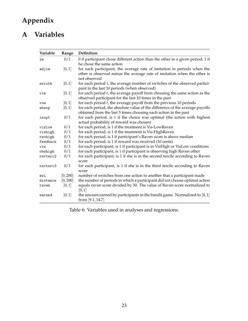
A Variables

Variable Range Definitionim 0/1 0 if participant chose different action than the other in a given period, 1 if

he chose the same actionadjim [0, 1] for each participant, the average rate of imitation in periods when the

other is observed minus the average rate of imitation when the other isnot observed

swioth [0, 1] for each period t, the average number of switches of the observed partici-pant in the last 10 periods (when observed)

vim [0, 1] for each period t, the average payoff from choosing the same action as theobserved participant for the last 10 times in the past

vow [0, 1] for each period t, the average payoff from the previous 10 periodsabsop [0, 1] for each period, the absolute value of the difference of the average payoffs

obtained from the last 5 times choosing each action in the pastisopt 0/1 for each period, is 1 if the choice was optimal (the action with highest

actual probability of reward was chosen)vislow 0/1 for each period, is 1 if the treatment is Vis-LowRavenvishigh 0/1 for each period, is 1 if the treatment is Vis-HighRavenravhigh 0/1 for each period, is 1 if participant’s Raven score is above medianfeedback 0/1 for each period, is 1 if reward was received (10 cents)vis 0/1 for each participant, is 1 if participant is in VisHigh or VisLow conditionsobshigh 0/1 for each participant, is 1 if participant is observing high Raven otherravterc2 0/1 for each participant, is 1 if she is in the second tercile according to Raven

scoreravterc3 0/1 for each participant, is 1 if she is in the third tercile according to Raven

scoreswi [0, 200] number of switches from one action to another that a participant madedistance [0, 200] the number of periods in which a participant did not choose optimal actionraven [0, 1] equals raven score divided by 30. The value of Raven score normalized to

[0, 1]earned [0, 1] the amount earned by participants in the bandit game. Normalized to [0, 1]

from [9.1, 14.7]

Table 6: Variables used in analyses and regressions.

23

B Additional Analyses

0.1

.2.3

.4.5

.6.7

.8

q1 novis q2 novis q3 novis q1 vis q2 vis q3 vis

High Raven other Low Raven other

+/- 1SE q# - terciles of Raven scores

Figure 6: The rate of imitation in Vis and Novis treatments by the terciles of the Raven score (q1- the lowest Raven score; q3 - the highest). Blue bars represent the high Raven other, the red bars- the low Raven other. Spikes are ±1 SE.

-.05

.05

.15

.25

crt1 novis crt2 novis crt1 vis crt2 vis

High Raven other Low Raven other

+/- 1SE crt# - below/above median CRT

Figure 7: The rate of imitation in Vis and Novis treatments by the median of the CRT score. Bluebars represent the high Raven other, the red bars - the low Raven other. Spikes are ±1 SE.

24

adjim

b/sevis –0.082*

(0.038)obshigh 0.075

(0.044)vis × obshigh 0.179**

(0.059)ravterc2 –0.012

(0.033)ravterc3 –0.031

(0.052)vis × ravterc2 0.073

(0.054)vis × ravterc3 0.128

(0.067)obshigh × ravterc2 0.034

(0.057)obshigh × ravterc3 0.087

(0.071)vis × obshigh × ravterc2 –0.074

(0.083)vis × obshigh × ravterc3 –0.257**

(0.090)cons 0.025

(0.023)

N 160

Table 7: OLS regression of adjusted imitation. Errors are robust. * – p < 0.05; ** – p < 0.01.

25

isopt Imitation Periods All Periodsb/se b/se

ravhigh 0.043* 0.035*(0.020) (0.014)

vishigh 0.067** 0.042**(0.021) (0.013)

vislow 0.007 0.025(0.024) (0.013)

ravhigh × vishigh –0.050 –0.027(0.033) (0.025)

ravhigh × vislow –0.026 –0.030(0.033) (0.025)

cons 0.666** 0.666**(0.014) (0.008)

N 32000 32000Indep. N 160 160

Table 8: Random effects OLS regression of optimality. Errors are clustered by session. * – p <0.05; ** – p < 0.01.

feedback

b/seravhigh 0.025**

(0.005)vislow 0.020*

(0.009)vishigh 0.042**

(0.009)ravhigh × vislow –0.017*

(0.008)ravhigh × vishigh –0.038**

(0.012)cons 0.582**

(0.007)

N 32000Indep. N 160

Table 9: Random effects OLS regression of earnings. Errors are robust. * – p < 0.05; ** – p < 0.01.

26

0.0

1.0

2.0

3D

ensi

ty

20 40 60 80 100Distance from optimal policy

Figure 8: The distribution of the values of the variable distance, the distance of participants’choices from optimal policy.

Adj

uste

d Im

itatio

n R

ate

Adj

uste

d Im

itatio

n R

ate

PeriodHigh Raven Participants

PeriodLow Raven Participants

-.2

-.15

-.1

-.05

0.0

5.1

.15

0 20 40 60 80 100

-.2

-.15

-.1

-.05

0.0

5.1

.15

0 20 40 60 80 100

Novis TreatmentsVis Treatments

NovisTreatmentsVis Treatments

Figure 9: Graphs of imitation rate by low and high Raven participants. Only graphs for lowRaven observed participants are shown. Ranges are ±1 SE.

27

C Experimental Instructions

The following is a translation of the original instructions in Italian. The experimenter read theinstructions aloud to the participants while they followed along their own copy. Original in-structions are available upon request. We decided to leave the instructions as is, which meansthat the numbering of figures in the instructions goes separately from the main text. In whatfollows, the numbers of figures refer only to figures in the instructions.

INSTRUCTIONSDear student you are about to participate in an experiment on decision making. Your privacyis guaranteed: results will be used and published anonymously. Your earnings will depend onyour performance in the experiment, according to the rules which we will explain to you shortly.You will be paid privately at the end of the experimental session. Other participants will not beinformed about your earnings. The maximum amount you can earn in the experiment is e 35.85and the minimum is e 3.10.

The experiment is divided in 3 parts. Each part of the experiment will be described in detailbelow.

Part OneCOMPLETION OF MATRICES PROBLEMSIn this task you will be ask to solve 30 different test items. In each test item we ask you to identifythe missing element that completes a pattern of shapes. The patterns are presented in the formof a 3x3 matrix. An example of a test item is shown here.

The shapes included in the matrix follow some regular patterns, for example, in the firstcolumn there is a circle, a rhombus and a square. In the second column there is a rhombus, asquare and a circle. In the third column there is a square and a circle. Therefore, the symbol thatcompletes the sequence in the third column is a rhombus.

28

You can identify regular patterns also by observing the shapes by row. For example in thefirst row each shape includes a dashed line. In the second row each shape includes two dashedlines, and in the third row each shape includes three dashed lines. Therefore, the symbol thatcompletes the sequence in the third row includes three dashed lines.

Regular patterns can be identified also by observing the shapes by diagonal. For example,in the first diagonal the dashed lines move from top-left to bottom-right, in the second diagonalthe dashed lines are vertical, in the third diagonal the dashed lines move from bottom-left totop-right, in the fourth diagonal the dashed lines move again from top-left to bottom right, andin the fifth diagonal the dashed lines are again vertical. Therefore, the symbol that completes thesequence in the third diagonal includes lines that move from bottom-left to top-right.

According to the patterns described above the shape that completes the matrix is number 5.A rhombus with three dashed lines that move from bottom-left to top-right.

You will have 20 minutes to complete the largest possible number of items and you will earn30 cents for each correct answer. If you do not complete an item or your answer is incorrect youwill earn 0 cents for that item.

In this part of the experiment, you can earn between e 0 and e 9.

Part TwoQUESTIONNAIRESSee Appendix E.

Part ThreeCHOICE TASKIn this part of the experiment you will face 200 trials divided in four blocks of 50 trials each.On each trial you will be asked to choose between two symbols. The two symbols are liketwo slot machines that give you a reward of 10 cents with a certain—unknown—probability (0otherwise). You do not have to pay before to choose your symbol and your goal will be to try tochoose the symbol that gives you the 10 cents with the highest probability. However, you do notknow the probability associated with the two symbols of getting the 10 cents, and you will needto figure out what is the most convenient symbol to play following the feedback you will receivefrom time to time. In fact, after choosing one of the two symbols you will be notified about theoutcome of your bet (if you have won 10 cents or 0 cents).

The experiment proceeds as follows:When a red silhouette appears on the screen (Figure 1), it means that you have to choose one ofthe two symbols. After you press the answer button your choice will appear under the selectedsymbol (Figure 2) and you will receive a feedback about the outcome of your choice (Figure 3appears if you have won 0 cents and figure 4 if you have won 10 cents).

29

Figure 1 Figure 2

Figure 3 Figure 4

Probability of winning associated with the two symbolsAt the beginning of the experiment a certain probability of winning will be associated with eachof the two symbols. The probability of winning will change slowly in the course of the experi-ment (Figure 5). For example, if at the beginning of the experiment the probability of receivingthe 10 cents is equal to 0.8 (you receive the reward 8 times out of 10), this probability may in-crease or decrease slightly in the subsequent trial and so on until the end of the experiment. It isimportant to keep in mind that the probabilities of winning associated with the two symbolsare independent, therefore if the probability of winning associated with one symbol increasesfrom one trial to the next, the probability of winning associated with the other symbol doesnot necessarily decrease.

Figure 5

Observational phaseIn addition to the feedback about the outcome of your choice, you will receive additional infor-mation during the experiment. Before making your choice, you often have the chance to observethe choice made (in the same trial) by a participant carrying out this same experimental task. Theonly difference between you and this participant is that he/she could not observe the actions ofanother participant. This participant will be represented with a green silhouette (Figure 6) andfrom time to time, before making your choice, you will see the choice made by this participant inthe trial you are about to play (Figure 7). After you have observed the choice of this participant,

30

you will make your decision.

Figure 6 Figure 7

Timeline of the experimental phasesAt the beginning of the experiment you will not see the choices made by the other participant.Then, in different time phases, and always before making your choice, you will see the choicemade by the other participant. The other participant had the same goal as you, which is tochoose the option that would guarantee the highest probability of winning.

In Figure 8 you can see a diagram that summarizes the experimental structure.

Figure 8

Random selection of the observed participant (Non-visible condition)The participant you will observe has completed (like you) all the parts of the experiment, includ-ing the questionnaire on matrices problems that you completed at the beginning of the exper-imental session. The chart below (Figure 9) shows the scores obtained by all participants whoparticipated in this study in the previous sessions (December 2015). The participant that youwill observe was selected among these 51 participants.

31

Figure 9 (version a)

Random selection of the observed participant (Visible low condition)The participant you will observe has completed (like you) all the parts of the experiment, includ-ing the questionnaire on matrices problems that you completed at the beginning of the experi-mental session. The chart below (Figure 9) shows the performance achieved by all participantswho participated in this study in the previous sessions (December 2015). The score achieved bythe participant that you will observe is colored in red.

Figure 9 (version b)

Random selection of the observed participant (Visible high condition)The participant you will observe has completed (like you) all the parts of the experiment, includ-ing the questionnaire on matrices problems that you completed at the beginning of the experi-mental session. The chart below (Figure 9) shows the performance achieved by all participantswho participated in this study in the previous sessions (December 2015). The score achieved bythe participant that you will observe is colored in red.

32

Figure 9 (version c)

D Holt and Laury Lotteries

The following figure shows how the Holt and Laury task was presented to the participants. Thepayoffs were identical to the payoffs in Holt and Laury (2002). The participants did not knowhow much they earned until the end of the experiment.

33

E Empathy Quotient

The Empathy Quotient consists of 60 questions aimed at assessing autistic traits. It is designedfor healthy adults (Baron-Cohen and Wheelwright, 2004). The questions can be found here:http://docs.autismresearchcentre.com/tests/EQ.pdf.

F Details of the Experiment

Date Number of ParticipantsExperiment 1

Dec 11, 2015 21Dec 14, 2015 16Dec 18, 2015 21

Experiment 2Novis

Jan 22, 2016 22Jan 22, 2016 20Feb 16, 2016 20Feb 16, 2016 12

VisJan 29, 2016 20Jan 29, 2016 12Feb 04, 2016 18Feb 04, 2016 20Feb 17, 2016 4Feb 17, 2016 14

Table 10: Summary of experimental sessions.

34