Observables from Correlation Functions

In this chapter we learn how to compute physical quantities from correlation functions

beyond leading order in the perturbative expansion. We will not discuss ultraviolet

divergences here; this important subject is left for the next chapter. We will illustrate

our results using quantum field theories in lower spacetime dimensions, which do not

have ultraviolet divergences.

1 Physical Mass

We begin with the mass of a particle. By itself this is not a very exciting observable,

but it is the first step in doing physical calculations beyond leading order in pertur-

bation theory. At tree level, this is just the coefficient of the φ2 term, but the at loop

level the two are no longer the same.

1.1 Mass Poles

We begin with the 2-point function in scalar field theory. We will show that 1-

particle intermediate states give rise to a pole singularity in the 2-point function at

the physical mass. This will allow us to give a precise definition of the physical mass.

The operator formulation tells us that

〈φ(x1)φ(x2)〉 = 〈0|T φ(x1)φ(x2)|0〉, (1.1)

where φ is the Heisenberg field operator, and |0〉 is the exact vacuum, i.e. the ground

state of the full interacting Hamiltonian. We write

〈0|T φ(x1)φ(x2)|0〉 = θ(x01 − x0

2)〈0|φ(x1)φ(x2)|0〉 + (1 ↔ 2). (1.2)

where

θ(t) =

{

1 if t > 0

0 otherwise.(1.3)

We now insert a complete set of states in each of the time orderings above. The

states we use are eigenstates of the full interacting Hamiltonian. These consist of the

vacuum, the 1-particle states, 2-particle states, etc:

1 = |0〉〈0|+∫ d3p

(2π)3

1

2E~p|~p 〉〈~p |

︸ ︷︷ ︸

1-particle states

+ 2-particle states + · · · , (1.4)

1

where

E~p = +√

~p2 + m2phys. (1.5)

Note that the physical mass appears because the 1-particle states are the eigenstates

of the full Hamiltonian.

Inserting Eq. (1.4) into Eq. (1.2) gives

〈0|T φ(x1)φ(x2)|0〉 =∫

d3p

(2π)3

1

2E~p〈0|φ(x1)|~p 〉〈~p |φ(x2)|0〉 + (1 ↔ 2) + · · · (1.6)

Here we assume that the vacuum expectation value of the field vanishes, i.e.

〈0|φ(x)|0〉 = 0. (1.7)

As long as we are dealing with a vacuum that is Lorentz invariant and translation

invariant, the vacuum expectation value is a constant, and we can work with shifted

fields for which Eq. (1.7) is satisfied. The leading contribution therefore arises from

the 1-particle states. We will show that these give rise to a pole at the physical mass.

We will later show that the contribution from states with 2 or more particles are

analytic near p2 = m2, so the 1-particle states give the complete pole structure.

We can simplify the matrix element by using translation invariance:

〈0|φ(x)|~p〉 = 〈0|eiPµxµ

φ(0)e−iPµxµ |~p 〉= 〈0|φ(0)|~p 〉e−ipµxµ

. (1.8)

Here Pµ is the physical 4-momentum operator that acts as the spatial- and time-

translation operator on states. In the last line, we have used the translation invariance

of the vacuum state to write P |0〉 = 0. From now on we leave p0 = E~p implicit for

brevity. We now use the fact that φ(0) is Lorentz invariant to write

〈0|φ(x)|~p 〉 = 〈0|U(L)φ(0)U †(L)|~p 〉e−ip·x

= 〈0|φ(0)|L−1~p 〉e−ip·x

= 〈0|φ(0)|~p = 0〉e−ip·x (1.9)

where U(L) is the unitary representation of the Lorentz transformation L on the

physical states, and we have chosen L−1~p = 0 in the last line. Substituting this into

Eq. (1.6) gives

〈0|φ(x1)φ(x2)|0〉 =∫

d3p

(2π)3

1

2E~pe−ip·(x1−x2)|〈0|φ(0)|~p = 0〉|2 + (1 ↔ 2) + · · · (1.10)

2

where the omitted terms come from the contribution from states containing 2 or more

particles. The constant matrix element

Zdef= |〈0|φ(0)|~p = 0〉|2 (1.11)

will play an important role in higher order corrections, as we will see below. This gives

the probability that the field operator φ creates a single particle state. (Of course,

this Z is completely different from the generating function of diagrams, also denoted

by Z.) Z = 1 in free field theory, but Z 6= 1 at higher orders in the pertubative

expansion.1

We can write the momentum integral in Eq. (1.10) in a manifestly Lorentz invari-

ant way using the identity∫

dω

2π

ie−iωt

ω2 − E2 + iǫ=

e−iE|t|

2E. (1.13)

This is a standard identity in quantum field theory that can be derived as follows.

The integrand has poles at ω = ±E ∓ iǫ. For t > 0, the ω integration contour can

be completed in the lower half plane, while for t > 0, the integral can be completed

in the upper half plane. The contribution from the residues gives the result above.

This gives

〈0|T φ(x1)φ(x2)|0〉 = Zθ(x01 − x0

2))∫

d4p

(2π)4e−ip·(x1−x2)

i

p2 − m2phys + iǫ

+ (1 ↔ 2) + · · · (1.14)

We recognize

∆phys(x1, x2) =∫ d4p

(2π)4e−ip·(x1−x2)

1

p2 − m2phys + iǫ

(1.15)

as the Feynman propagator with the mass given by the physical mass. We therefore

have

〈0|T φ(x1)φ(x2)|0〉 = iZ∆phys(x1, x2) + · · · . (1.16)

1In fact, an argument similar to the given above can be used to show that Z < 1 in any interacting

theory. The argument proceeds by starting with the vacuum expectation value of the canonical

commutation relation and inserting a complete set of states. In a free field theory this is saturated

by the 1-particle states, and we get Z = 1. In an interacting theory, higher particle states contribute,

and we get Z < 1. Because Z is manifestly positive, we conclude that

0 < Z < 1. (1.12)

3

In momentum space, we see that the 2-point function has a pole at the physical mass.

We have not discussed the contribution from states containing 2 or more particles,

but it can be shown that they do not give rise to poles.

This result is important because it gives us a definition of the physical mass that

is useful for calculations: the mass is the pole in the 2-point function. For this reason,

the physical mass is sometimes referred to as the ‘pole mass.’

1.2 The 1PI 2-Point Function

Consider the momentum space 2-point function with external propagators removed

(‘amputated’). This is given by a sum of diagrams. A given diagram is called ‘1

particle irreducible’ (1PI) if it cannot be cut into two disconnected pieces by cutting

a single internal line. For example,

(1.17)

is 1PI, while

(1.18)

is not, since it can be cut in half as shown. To emphasize that the external lines have

been amputated, we have put a small slash on them. For example, this reminds us

that we cannot cut a diagram in half by cutting an external line. We denote the sum

of all 1PI 2-point graphs as

= −iΣ(p2). (1.19)

For example, the diagrammatic expansion of Σ in φ4 theory is

−iΣ = + + + O(λ2). (1.20)

We can express the full connected 2-point function (including external lines) in

terms of the 1PI 2-point function as follows:

= + + + · · · (1.21)

4

=i

p2 − m2+

(

i

p2 − m2

)2 (

−iΣ(p2))

+

(

i

p2 − m2

)3 (

−iΣ(p2))2

+ · · · (1.22)

Factoring out one propagator, we see that this is a geometric series:

=i

p2 − m2

∞∑

n=0

(

Σ(p2)

p2 − m2

)n

=i

p2 − m2

[

1 − Σ(p2)

p2 − m2

]−1

. (1.23)

Putting all terms over a common denominator gives

=i

p2 − m2 − Σ(p2). (1.24)

This result is sometimes called Dyson’s formula.2 It is an important result: it

tells us that the 1PI corrections can be resummed to appear as a correction to the

denominator of the full 2-point function.

1.3 Diagrammatic Expansion of the Physical Mass

To find the relation between Σ and the physical mass, we expand the denominator of

the Dyson formula around p2 = m2phys:

p2 − m2 − Σ(p2) = p2 − m2 −[

Σ(m2phys) + Σ′(m2

phys)(p2 − m2

phys)

+O((p2 − mphys)2)]

=[

1 − Σ′(m2phys)

]

(p2 − m2phys) + O((p2 − mphys)

2). (1.25)

The terms we have omitted do not contribute to the pole. Demanding that the pole

is at p2 = m2phys requires

m2phys = m2 + Σ(p2 = m2

phys). (1.26)

2Because the convergence of the series Eq. (1.23) may be in doubt, we should really take Eq. (1.24)

as the definition of Σ. Reversing the argument above, we conclude that Σ is given by the sum of all

1PI diagrams.

5

Expanding both sides of this relation in powers of the coupling gives the perturba-

tive expansion of the physical mass. Note that m2phys appears on both sides of the

expansion, but we can write

m2phys = m2 + m2

1λ + m22λ

2 + · · · (1.27)

and expand both sides in powers of λ to obtain the coefficients m21, m2

2, etc.

Using the identification Eq. (1.26), we can write Eq. (1.25) as

p2 − m2 − Σ(p2) =[

1 − Σ′(p2 = mphys)]

(p2 − m2phys) + O((p2 − mphys)

2). (1.28)

The coefficient of the pole is therefore

Z =1

1 − Σ′(p2 = m2phys)

. (1.29)

2 An Example Calculation

We now illustrate the results above for the 2-point function with a loop calculation.

We will calculate mphys and Z in scalar field theory with a potential

V (φ) =1

2m2φ2 +

λ

3!φ3. (2.1)

This potential is unbounded from below (for any sign of m2 or λ), and it is not clear

whether the theory is consistent.3 Nevertheless, we will use it as a simple model

to illustrate perturbative calculations. Furthermore, in order to avoid ultraviolet

divergences, we will work in 2+1 spacetime dimensions. In order to see the necessicity

of going to lower dimensions, we will keep the spacetime dimension d arbitrary to

begin with.

The leading contribution to the 1PI correlation function in momentum space is

−iΣ(p2) =

=1

2(−iλ)2

∫ddk

(2π)d

i

(k + p)2 − m2 + iǫ

i

k2 − m2 + iǫ. (2.2)

3For m2 > 0 there is a local minimum at φ = 0, and the field must tunnel through a poten-

tial barrier in order to access the lower energy states. The lifetime of the ‘metastable vacuum’ is

exponentially long if λ is small, and may be long enough to be interesting.

6

Notice that for large k, we can approximate both of the propagators by 1/k2. The

large k region of integration therefore behaves like

∫ddk

(2π)d

1

k4. (2.3)

This diverges for d ≥ 4, so the expression Eq. (2.2) is ill-defined for these values of d.

We will discuss how to deal with this situation in detail later. For now we want to

avoid this complication, so we simply take d = 3.

We now introduce some tricks (also due to Feynman) for calculating loop integrals

such as Eq. (2.2).

• Combine denominators: We use the identity

1

AB=∫ 1

0dx

1

(xA + (1 − x)B)2(2.4)

to write the integral in terms of a single denominator. This is called a Feynman

parameter integral. In the present case, we have

denominator = x(k2 + 2p · k + p2 − m2 + iǫ) + (1 − x)(k2 − m2 + iǫ)

= k2 + 2xp · k + xp2 − m2 + iǫ

= K2 − M2 + iǫ, (2.5)

where

K = k + xp, M2 = m2 − x(1 − x)p2. (2.6)

• Shift the momentum integral: Writing the integral in terms of the shifted variable

K, we have

Σ(p2) =iλ2

2

∫ 1

0dx∫

d3K

(2π)3

1

(K2 − M2 + iǫ)2. (2.7)

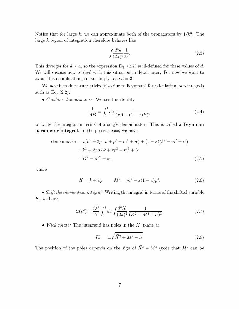
• Wick rotate: The integrand has poles in the K0 plane at

K0 = ±√

~K2 + M2 − iǫ. (2.8)

The position of the poles depends on the sign of ~K2 + M2 (note that M2 can be

7

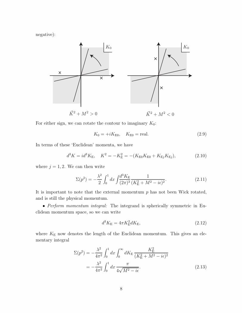
negative):

For either sign, we can rotate the contour to imaginary K0:

K0 = +iKE0, KE0 = real. (2.9)

In terms of these ‘Euclidean’ momenta, we have

d3K = id3KE, K2 = −K2E = −(KE0KE0 + KEjKEj), (2.10)

where j = 1, 2. We can then write

Σ(p2) = −λ2

2

∫ 1

0dx∫

d3KE

(2π)3

1

(K2E + M2 − iǫ)2

. (2.11)

It is important to note that the external momentum p has not been Wick rotated,

and is still the physical momentum.

• Perform momentum integral: The integrand is spherically symmetric in Eu-

clidean momentum space, so we can write

d3KE = 4πK2EdKE, (2.12)

where KE now denotes the length of the Euclidean momentum. This gives an ele-

mentary integral

Σ(p2) = − λ2

4π2

∫ 1

0dx∫ ∞

0dKE

K2E

(K2E + M2 − iǫ)2

= − λ2

4π2

∫ 1

0dx

π

4√

M2 − iǫ. (2.13)

8

We have obtained the loop integral in terms of a Feynman parameter integral:

Σ(p2) = − λ2

16π

∫ 1

0dx

[

m2 − x(1 − x)p2 − iǫ]−1/2

. (2.14)

These steps (combining denominators, Wick rotating, and performing the momen-

tum integrals) can be straightforwardly carried out for any diagram. Performing the

Feynman parameter integrals is difficult in general, although we can do it for this

simple example.

The iǫ factor is important for resolving the poles if the term in square brackets is

negative. Using the fact that max [x(1 − x)] = 14, we see that this occurs only if

p2 ≥ 4m2. (2.15)

This is precisely the condition that p2 is large enough to allow the production of a

pair of particles of mass m. (Note that p2 is the square of the center of mass energy.)

That is, if p2 ≥ 4m2, the momenta of the intermediate lines can satisfy k2 = m2,

(k + p)2 = m2; in this case, we say that the momenta in the loop are on shell. As

long as p2 < 4m2 we can ignore the iǫ factor, and the integrand is manifestly real and

analytic in p2. In particular, the fact that it is real near p2 = m2 is crucial in order

for us to interpret it as a correction to the physical mass. For p2 ≥ 4m2, singularities

can (and do) appear. This is a particular case of an important general result: loop

diagrams have singularities in momentum space in regions where the momenta of the

intermediate lines can go on shell.

It may appear that the connection between the singularities of the correlation

functions and the existence of real intermediate states is violated by the fact that m2

is not the physical mass. However, we will see that it is possible to reorganize the

perturbative expansion so that the propagator used in perturbation theory has poles

at p2 = m2phys. We will show below that in this ‘renormalized’ expansion, singularities

of correlation functions are always due to real intermediate states.

To evaluate the integral Eq. (2.14), we scale out the m dependence by writing

Σ(p2) = − λ2

16πm

∫ 1

0dx [1 − x(1 − x)z]−1/2 , (2.16)

where

z =p2 + iǫ

m2. (2.17)

Performing the integral, we obtain

Σ(p2) = − λ2

16π

1√p2 + iǫ

ln1 +

√

p2/4m2 + iǫ

1 −√

p2/4m2 + iǫ. (2.18)

9

This function is not singular at p2 = 0 because the singularity in the prefactor is

cancelled by the zero of the logarithm:

Σ(p2) = − λ2

16πm

[

1 +p2

6m2+ O(p4)

]

. (2.19)

There is a branch cut singularity when 2m +√

p2 + iǫ goes to zero, which occurs at

p2 = 4m2 − iǫ. (2.20)

In the complex p2 plane, the singularity structure looks like

The iǫ tells us that the singularity should be approached from the direction of positive

imaginary p2. In this example, there are no singularities in the entire complex p2 plane

other than those from real intermediate states Later, we will prove that this result is

general if we restrict to real external momenta.

We complete our treatment of this example by computing mphys and Z. To com-

pute mphys, we need to find the position of the pole in the full 2-point function. We

must therefore solve

p2 − m2 − Σ(p2)∣∣∣p2 = m2

phys

= 0. (2.21)

Since m2phys = m2 + O(λ2), we can write

m2phys = m2 + Σ(m2) + O(λ4). (2.22)

To evaluate Σ(m2), we can ignore the iǫ factor and obtain

Σ(m2) = − λ2

16πm

∫ 1

0dx [1 − x(1 − x)]−1/2

= − λ2

16πmln 3. (2.23)

10

We see that the loop corrections make the physical mass smaller than m2.

We can also compute Z using Eq. (1.29). To the order we are working, we have

Z = 1 + Σ′(m2) + O(λ4), (2.24)

where Σ′(p2) = ∂Σ(p2)/∂p2. Using Eq. (2.14), we have

Σ′(p2) = − λ

32π

∫ 1

0dx x(1 − x)

[

m2 − x(1 − x)p2 − iǫ]−3/2

. (2.25)

Therefore,

Σ′(m2) = − λ2

32πm3

∫ 1

0dx x(1 − x) [1 − x(1 − x)]−3/2 (2.26)

= − λ2

32πm3

(4

3− ln 3

)

. (2.27)

Note that 43− ln 3 ≃ 0.23 > 0, so Z < 1, as expected. (In fact, the Feynman integral

in Eq. (2.26) is manifestly positive.)

2.1 Mass Renormalization

For some purposes, it is convenient to define the diagrammatic expansion so that the

mass in the propagator is the same as the physical mass to all orders in perturbation

theory. To do this, we write

m2 = m2phys + ∆m2 (2.28)

and note that ∆m2 starts at higher orders in the loop expansion. Here, m2 is the

mass parameter that appears in the Lagrangian, sometimes called the bare mass.

As discussed previously, the loop expansion can be viewed as an expansion in

powers of h, so ∆m2 = O(h) is a quantum correction. We then expand systematically

in powers of h, treating m2phys as O(h0). We therefore write the Lagrangian as

L = Lren + ∆L, (2.29)

where

Lren = 12∂µφ∂µφ − 1

2m2

physφ2 +

λ

3!φ3 (2.30)

is the ‘renormalized’ Lagrangian and

∆L = −12∆m2φ2 (2.31)

11

is a ‘counterterm’ Lagrangian. Because ∆L is treated as an O(h) perturbation, it

gives rise to a new Feynman rule:

= −i∆m2. (2.32)

This is to be regarded as a two-point vertex. The square dot on the vertex reminds

us that it is a counterterm. The expansion of the 1PI 2-point function to O(h) is

therefore

−iΣ = + + O(h2), (2.33)

where the counterterm ∆m2 is determined by the condition that mphys is the physical

mass. In equations, this is

Σ(p2 = m2phys) = 0. (2.34)

By imposing this renormalization condition order by order in the h expansion, we

ensure that mphys is the physical mass at each order in perturbation theory. In this

perturbative expansion, the Feynman propagator is

∆(x1, x2) =∫

d4p

(2π)4

ie−ip·(x1−x2)

p2 − m2phys + iǫ

(2.35)

to all orders in perturbation theory. The original theory was defined by two param-

eters, λ and m2. In the ‘renormalized’ perturbative expansion, we have traded the

parameter m2 for m2phys. The condition Eq. (2.35) determines ∆m2 order by order in

the expansion, so it is not an independent parameter.

In this way of organizing the perturbative expansion, the position of the poles

in the propagators coincide with the physical poles. This is convenient for proving

unitarity from the diagrammatic expansion, as we will discuss below.

2.2 Tadpole Condition

There is another diagram that contributes to the 2-point function at O(λ2), namely

(Although this diagram can be cut into two parts by cutting the internal line, it

contributes to Σ because of Eq. (1.21).) Associated with this is a contribution to the

1-point function

= −iλ

2

∫ d3k

(2π)3

i

k2 − m2 + iǫ(2.36)

12

A diagram like this that contributes to the 1-point function is called a tadpole

diagram for obvious reasons. This integral is ill-defined because it diverges at large

k, and therefore the contribution to the 2-point function is also ill-defined.

To understand what is going on, note that we can get a tree-level contribution to

the 1-point function by adding a linear term in φ to the Lagrangian:

∆L = −κφ. (2.37)

This term is allowed by all symmetries, and there is no reason not to add it. (Since

the interaction already contains a φ3 term, we cannot forbid this by imposing φ 7→ −φ

symmetry.) This term would give rise to a 1-point vertex in the Feynman rules:

= −iκ (2.38)

This would also contribute to the 1-point function. The significance of this term is

clearer if we consider the full potential:

V (φ) = κφ + 12m2φ2 +

λ

3!φ3. (2.39)

This potential is minimized at φ = v, where

v = −m2 −√

m4 − 2λκ

λ, (2.40)

assuming that m4 ≥ 2λκ. (If m4 < 2λκ the potential has no stationary points.)

Expanding around φ = v,

φ = v + φ′, (2.41)

the potential is

V (φ′) = 12m′2φ′2 +

λ

3!φ′3, (2.42)

where m′2 = m2 + λv. We see that expanding about φ = v gives a theory with no

linear term in the potential. The value of κ can be absorbed into a shift in the field.

We see that demanding that the potential be extremized is equivalent to demand-

ing the absence of a tadpole at tree level. It is therefore natural to impose the tadpole

condition

13

3 Analyticity of Feynman Amplitudes

We address the question of the location of the singularities of Feynman diagrams such

as the example above. By a ‘singularity,’ we mean any point where the amplitude is

not analytic as a function of external momenta. We therefore consider a branch point

as a singularity, even though the amplitude does not blow up there. We will show

here that all singularities of Feynman diagrams are associated with the appearance of

real intermediate states. We might expect that a Feynman diagram has a singularity

whenever any one of the internal propagators can go on-shell. However, in most cases

we can deform the integral in the complex plane to avoid the singularity. A singularity

can occur only if the integrand has a singularity that cannot be avoided.

Let us see how this works for integrals of the form

I(x) =∫ b

adz

N(x, z)

D(x, z), (3.1)

where N and D are analytic in a neighborhood that includes the real interval a ≤ z ≤b and a region around the x values of interest. An analytic function can be written as

a convergent power series, and therefore the integrand is singular only at zeros of D.

(Note that the Feynman parameter integral in Eq. (2.14) is not of this form because

the denominator has a square-root singularity in the physical region.) Suppose that

for D(x, z) = 0 for some a < z < b, but ∂zD(x, z) 6= 0. Then we can deform the

contour in the complex z plane to avoid the singularity, and I(x) is nonsingular at

x = x. The only singularities of I(x) result from singularities of the integrand that

cannot be avoided by deforming the z contour of integration. This happens in one of

the following two cases:

• Singularities at the endpoints, i.e. D(x, a) = 0 or D(x, b) = 0.

• “Pinch” singularities where a zero approaches the the real z axis from both sides

as x → x. This occurs if D has a double zero in z:

D(x, z) = 0 and ∂zD(x, z) = 0. (3.2)

To see this, we expand D about z = z, x = x:

D(x, z) = A(z − z)2 + B(x − x)n + · · · (3.3)

for some A and B and integer n ≥ 1. In the approximation where we neglect higher

order terms, D has zeros at

z = z ±√

B

A(x − x)n. (3.4)

14

To move the singularity off the real z axis, we must choose the phase of x − x so

that the square root has a nonzero imaginary part. But then there are two zeros that

“pinch” the real z axis from both sides as x → x.

Some simple examples:

I(x) =∫ 1

0

dz

z + x= ln

1 + x

x. (3.5)

The denominator has a simple zero when z+x = 0, but this is an avoidable singularity

unless it is at an endpoint, that is x = 0 or x = −1. We see that this does account

for the singular points of the integral. Note that the singularity is a branch cut

singularity. We can move the branch cut by using a different branch of the logarithm,

but we cannot move the branch points. Another example is

I(x) =∫ ∞

−∞

dz

z2 + x=

π√x. (3.6)

The integrand has a pinch singularity when x → 0, and indeed it is singular there.

We can extend this to multiple integrals of the form

I(x1, . . . , xm) =∫ b1

a1

dz1 · · ·∫ bn

an

dznN(x1, . . . , xm, z1, . . . , zn)

D(x1, . . . , xm, z1, . . . , zn), (3.7)

where N and D are analytic in a nighborhood that includes the real intervals ai ≤zi ≤ bi for i = 1, . . . , n and the values of x1, . . . , xm that are of interest. In this

case, we must have either a pinch or endpoint singularity in each integration variable

zi. The condition for a singularity is that there are points x1, . . . , xm, z1, . . . , zn,

with ai ≤ zi ≤ bi such that D(x, z) = 0 and for each zi we have either an endpoint

singularity (zi = ai or bi) or a pinch singularity: ∂ziD(x, z) = 0.

For example, consider the integral

I(x) =∫ 1

−1dz1

∫ ∞

−∞dz2

1

z1 + z22 + x

= 2π(√

1 + x −√

1 − x)

. (3.8)

As x → 0, the denominator of the integrand vanishes for z1 = z2 = 0. It is a pinch

singularity in z2, but it is avoidable in z1. Therefore, there is no singularity of I(x)

at x = 0. For x = ±1, the denominator vanishes for z1 = ±1, z2 = 0. This is an

endpoint singularity in z1 and a pinch singularity in z2, so we expect a singularity

there. The conditions for the singularity are therefore

Let us now apply this to a general Feynman diagram. A diagram with E external

legs, I internal legs, and L loops can be written in the form

M(p1, . . . , pE) =∫

d4k1 · · · d4kL N(p1, . . . , pE, k1, . . . , kL)

× 1

q21 − m2

1 + iǫ· · · 1

q2I − m2

I + iǫ. (3.9)

15

Here p1, . . . , pE are external momenta, k1, . . . kL are the loop momenta, and q1, . . . , qI

are the momenta on the internal lines. The function N is a polynomial in the mo-

menta arising from possible derivative couplings. (We assume that the amplitude is

amputated, so there are no poles associated with external lines.) The internal mo-

menta are linear combinations of the external momenta and the loop momenta that

depend on the topology of the diagram. We can combine the denominators using the

Feynman identity

1

D1 · · ·DI=∫ 1

0dx1 · · ·

∫ 1

0dxI δ(x1 + · · ·+ xI − 1)

1

DI, (3.10)

where

D = x1D1 + · · · + xIDI . (3.11)

We therefore obtain

M(p) =∫

d4k1 · · · d4kL

∫ 1

0dx1 · · ·

∫ 1

0dxI δ(x1 + · · ·xI − 1)

N(p, k)

[D(x, q)]I, (3.12)

where

D(x, q) = x1(q21 − m2

1 + iǫ) + · · · + xI(q2I − m2

I + iǫ). (3.13)

For purposes of discussing the analyticity structure of the diagram, the delta function

is not very convenient. We can eliminate it using the following trick. First, note that

there is no harm in extending the range of the x integrals from 0 to ∞, since the

delta function determines the range in any case. We then change variables xi → xi/λ

where λ is a positive constant. This gives

M(p) = λ∫

d4k1 · · ·d4kL

∫ ∞

0dx1 · · ·

∫ ∞

0dxI δ(x1 + · · ·xI − λ)

N(p, k)

[D(x, q)]I, (3.14)

where the factor of λ arises from the delta function. Since M is independent of λ,

we can write

M(p) =∫ ∞

0dλ e−λM(p) (3.15)

=∫ ∞

0dλ, e−λ λ

∫

d4k1 · · · d4kL

∫ ∞

0dx1 · · ·

∫ ∞

0dxI

× δ(x1 + · · ·xI − λ)N(p, k)

[D(x, q)]I

=∫

d4k1 · · ·d4kL

∫ ∞

0dx1 · · ·

∫ ∞

0dxI

Xe−XN(p, k)

[D(x, q)]I, (3.16)

16

where

X = x1 + · · ·+ xI . (3.17)

The integrand in Eq. (3.16) has singularities only when the denominator vanishes,

and the denominator is a polynomial in the integration variables, so we can directly

apply the criteria above to find the singularities.

In order to have a singularity, the integral must have an endpoint or pinch singu-

larity in each of the 4L + I integrals. This means that for some value of the external

momenta p and integration variables k and x we have D(x, q) = 0, such that the

following conditions are satisfied.

• For each Feynman parameter integral over xi (i = 1, . . . , I), either

xi = 0 (3.18)

or

0 =∂

∂xiD(x, q) = q2

i − m2, (3.19)

i.e.

q2i = m2

i . (3.20)

Note that if Eq. (3.18) or Eq. (3.20) is satisfied for all i, then D(x, q) = 0, so we

need not impose this condition independently.

• For each loop integral over kℓ (ℓ = 1, . . . , L) we must have a pinch singularity, since

there are no endpoints to the integral. This means that

0 =∂

∂kℓµD(x, q) = 2

I∑

i=1

xiqνi

∂qiν

∂kℓµ

∣∣∣∣∣q=q

. (3.21)

The partial derivatives satisfy

∂qiν

∂kℓµ= Ciℓδ

µν , (3.22)

where Ciℓ = 0 or ±1. This is because each loop momentum goes through a given

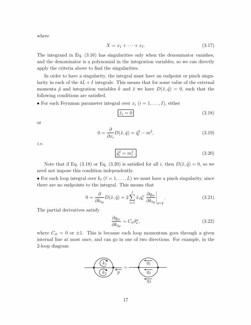
internal line at most once, and can go in one of two directions. For example, in the

2-loop diagram

=

17

we have q1 = p − k1, q2 = k1 − k2, q3 = k2. We can therefore restrict the sum

Eq. (3.21) to the internal lines i with Ciℓ 6= 0. The coefficients Ciℓ = ±1 then just

tell us whether qi is going in the same direction or the opposite direction of the loop,

and we can write the condition as

∑

any loop

xiqiµ = 0. (3.23)

In the 2-loop example above, we have two loop conditions:

x1q1 − x2q2 = 0,

x2q2 − x3q3 = 0.(3.24)

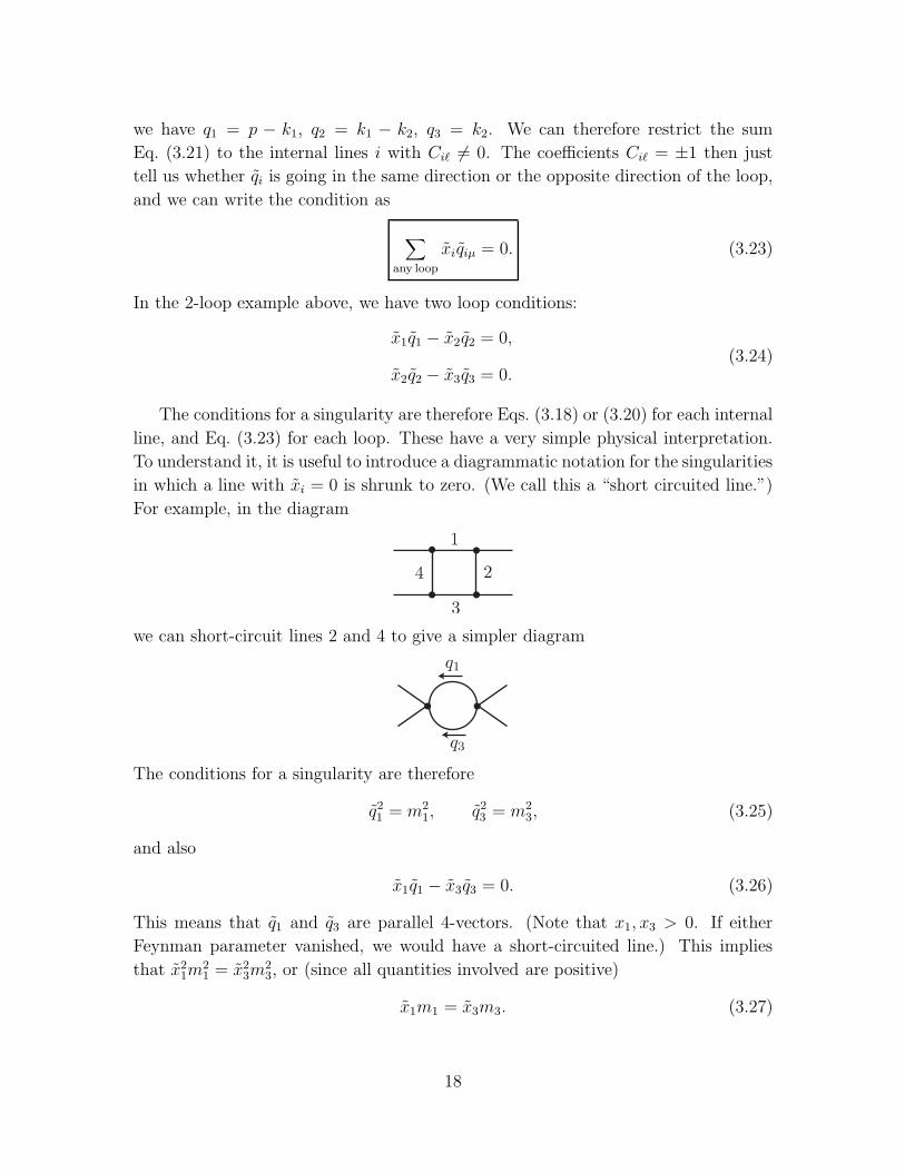
The conditions for a singularity are therefore Eqs. (3.18) or (3.20) for each internal

line, and Eq. (3.23) for each loop. These have a very simple physical interpretation.

To understand it, it is useful to introduce a diagrammatic notation for the singularities

in which a line with xi = 0 is shrunk to zero. (We call this a “short circuited line.”)

For example, in the diagram

we can short-circuit lines 2 and 4 to give a simpler diagram

The conditions for a singularity are therefore

q21 = m2

1, q23 = m2

3, (3.25)

and also

x1q1 − x3q3 = 0. (3.26)

This means that q1 and q3 are parallel 4-vectors. (Note that x1, x3 > 0. If either

Feynman parameter vanished, we would have a short-circuited line.) This implies

that x21m

21 = x2

3m23, or (since all quantities involved are positive)

x1m1 = x3m3. (3.27)

18

The location of the singularity is therefore

s = (q1 + q3)2 = (m1 + m3)

2. (3.28)

Therefore, the condition for the appearance of a singularity is that there is enough

energy to produce the particles 1 and 3.

Note that for any diagram, there is a trivial solution where all the internal lines

are short-circuited, i.e. x1 = · · · = xI = 0. We can show that this does not give rise

to a singularity by modifying Eq. (3.15) to read

M(p) = eǫ∫ ∞

ǫdλ e−λM(p) (3.29)

= eǫ∫

d4k1 · · · d4kL

∫ ∞

0dx1 · · ·

∫ ∞

0dxI θ(X − ǫ)

Xe−XN(k, p)

[D(x, q)]I. (3.30)

The left-hand side is independent of ǫ, but for any ǫ > 0, the integrand vanishes when

x1 = · · · = xI = 0. We conclude that at least one of the Feynman parameters must

be nonzero in order to have a singularity. (The θ function does not eliminate the

singularities where some of the xi are nonzero, since the conditions Eq. (3.23) that

determine the xi do not determine the overall scale.)

So far, the conditions apply even for complex external momenta. For real external

momenta, we can show that all singularities are associated with the production of

particles in the intermediate states. In fact, the conditions above imply that the

graph can be read as a picture of classical particles moving in spacetime, with all

momenta real and on mass shell, and all particles moving forward in time. This is

the Coleman-Norton theorem. To prove it, associate with each internal line a

spacetime separation

∆µi = xiq

µi . (3.31)

Since all the xi and qi are real, this is real. It also satisfies the consistency condition

∑

any loop

∆µi = 0. (3.32)

For any non-short circuited line, the particles are on mass shell. For a short-circuited

line, xi = 0 implies ∆µi = 0, so the particle exists for zero time. (We can think of

this as a classically allowed interaction mediated by the particle.) To see that the

particles propagate forward in time, note that the spacetime interval associated with

a classical particle with momentum qi is

∆µi = τi

qµi

mi, (3.33)

19

where τi is the proper time. Comparing with the definition Eq. (3.31), we see that

τi = ximi > 0, (3.34)

so the particle does indeed move forward in time.

Let us use these rules to analyze the singularities of the 1PI 2-point function Σ(p2).

The graphs that contribute have the form

In this diagram, the vertex on the right connects the external line to n internal lines,

and the vertex on the right connects to m internal lines. To be continued....

4 LSZ Reduction

We now show how to use these ideas to relate correlation functions to S matrix el-

ements. Let us recall some basic ideas of scattering theory. A physical scattering

experiment involves initial and final states consisting of well-separated wavepackets.

Because the initial and final state wavepackets are separated, we can neglect interac-

tions between them at sufficiently late and early times. The initial and final states

can therefore be treated as energy eigensstates of a free theory; we call these ‘in’

states and ‘out’ states. Since we are working in Heisenberg picture, the states are

independent of time and the fields evolve. Therefore, the information about the ini-

tial and final states is contained in free field operators φin and φout. The S matrix is

relation between the in and out fields:

φout = SφinS†. (4.1)

As we have seen above, the interacting Heisenberg field operators φ do not create

1-particle states with unit probability as free fields do. The probability to create a

single particle state is given by the Z factor of Eq. (1.11), so we have

φ(x)x0→−∞−→

√Z φin(x), φ(x)

x0→+∞−→√

Z φout(x). (4.2)

Here φin and φout are free fields acting on an ‘in’ and ‘out’ Fock space, respectively.

Now consider the momentum-space correlation function

(2π)4δ4(p1 + · · ·+ pn)G(n)(p1, . . . , pn)

=∫

d4x1 · · ·∫

d4xn eip1·x1 · · · eipn·xn〈0|T φ(x1) · · · φ(xn)|0〉.(4.3)

20

Using the same type of reasoning used for the 2-point function, we will show that this

correlation function has poles corresponding to matrix elements of 1-particle states.

To see this, consider the region of integration where x01 ≫ x0

2, . . . , x0n. In this

regime, we can replace

〈0|T φ(x1) · · · φ(xn)|0〉 → 〈0|√

Zφout(x1)T φ(x2) · · · φ(xn)|0〉

=∫

d3k

(2π)3

√Z

2E~k

e−ik·x1out〈~k|T φ(x2) · · · φ(xn)|0〉 + · · · , (4.4)

where the omitted terms come from states with 2 or more particles. Substituting this

into Eq. (4.3), the x01 integral is

∫ +∞

Tdx0

1 eip1,0x01e−iE~k

x01 =

i

p1,0 − E~k

ei(p1,0−E~k)T , (4.5)

where T = max{x02, . . . , x

0n}. The ~x1 integral is

∫

d3x1 e−i~p1·~x1ei~k·~x1 = (2π)3δ3(~k − ~p1). (4.6)

We therefore obtain a contribution to the momentum-space correlation function

(2π)4δ4(p1 + · · · + pn)G(n)(p1, . . . , pn)

=

√Z

2E~p1

i

p1,0 − E~p1

∫

d4x2 · · ·∫

d4xn eip2·x2 · · · eipn·xn

× out〈~p1|T φ(x2) · · · φ(xn)|0〉 + · · ·

(4.7)

Note that near p1,0 = E~p1,

1

2E~p1

i

p1,0 − E~p1

=i

p2 − m2phys

+ non-pole, (4.8)

so we have identified a pole term in the momentum-space correlation function:

(2π)4δ4(p1 + · · · + pn)G(n)(p1, . . . , pn)

p1,0→+E~p1−→ i√

Z

p21 − m2

phys

∫

d4x2 · · ·∫

d4xn eip2·x2 · · · eipn·xn

× out〈~p1|T φ(x2) · · · φ(xn)|0〉.

(4.9)

It can be shown that states containing 2 or more particles and other regions of inte-

gration do not give rise to a pole at p1,0 → +E~p1.

21

Let us now consider the region of integration x01 ≪ x0

2, . . . , x0n. In this regime, we

can replace

〈0|T φ(x1) · · · φ(xn)|0〉 → 〈0|[

T φ(x2) · · · φ(xn)]√

Zφin(x1)|0〉

=∫

d3k

(2π)3

√Z

2E~k

e+ik·x1〈0|T φ(x2) · · · φ(xn)|~k〉in + · · · . (4.10)

Repeating the steps above, we find that the momentum-space correlation function

has a pole at p1,0 → −E~p1:

(2π)4δ4(p1 + · · · + pn)G(n)(p1, . . . , pn)

p1,0→−E~p1−→ i√

Z

p21 − m2

phys

∫

d4x2 · · ·∫

d4xn eip2·x2 · · · eipn·xn

× 〈0|T φ(x2) · · · φ(xn)|~p1〉in.

(4.11)

We see that poles at positive (negative) energy correspond to incoming (outgoing)

states.

We can continue in this way, identifying poles in each of the momenta with in-

coming or outgoing states. We obtain

(2π)4δ4(p1 + · · ·+ pn)G(n)(p1, . . . , pn)

→ i√

Z

p21 − m2

phys

· · · i√

Z

p2n − m2

physout〈~p1, . . . ~pr|~pr+1, . . . , ~pn〉in

(4.12)

in the limit

p1,0 → +E~p1, . . . , pr,0 → +E~pr

pr+1,0 → −E~pr+1, . . . , pn,0 → −E~pn .

(4.13)

Eq. (4.12) is the LSZ reduction formula, due to Lehmann, Symanzyk, and Zim-

merman.

The matrix element in Eq. (4.12) is precisely an S matrix element:

out〈~p1, . . . , ~pr|~pr+1, . . . , ~pn〉in = 〈~p1, . . . , ~pr|S|~pr+1, . . . , ~pn〉. (4.14)

It is conventional to write

S = 1 + iT , (4.15)

22

and to define the invariant amplitude M by

(2π)4δ4(p1 + · · · + pn)M = 〈~p1, . . . , ~pr|T |~pr+1, . . . , ~pn〉. (4.16)

In terms of diagrams, we know that the momentum-space correlation function is

written in terms of amputated diagrams multiplied by propagator corrections:

(2π)4δ4(p1 + · · · + pn)G(n)(p1, . . . , pn) =Amp

...

p1

p2 pn

=i

p21 − m2 − Σ(p2

1)· · · i

p2n − m2 − Σ(p2

n)

× (2π)4δ4(p1 + · · ·+ pn)G(n)amp(p1, . . . , pn) (4.17)

→ iZ

p21 − m2

phys

· · · iZ

p2n − m2

phys

× (2π)4δ4(p1 + · · ·+ pn)G(n)amp(p1, . . . , pn), (4.18)

where we take the on-shell limit in the last line. Comparing this with Eq. (4.16),

we see that up to the factors of Z, M is just the amputated correlation function

evaluated on shell:

iM =(√

Z)n

G(n)amp

∣∣∣on shell

, (4.19)

where the sign of the 0 component of the 4-momenta determines whether the corre-

sponding state is incoming or outgoing (see Eq. (4.12)). This is our final result for

expressing S-matrix elements in terms of correlation functions.

The factors of√

Z in Eq. (4.19) can be understood from the fact that the S-matrix

should not depend on rescaling of the field variable in the path integral. Consider the

change of variables in the path integral

φ = cφ′, (4.20)

where c is a constant. Since this is just a change of variables, physical quantities such

as S matrix elements should not be affected. Both G(n)amp and Z in Eq. (4.19) depend

on c, but it is not hard to see that the dependence cancels.

Exercise: Check that the c dependence cancels in Eq. (4.19) using the Feynman

rules to deduce how G(n) and Z depend on c.

23

5 Unitarity

Unitarity of the S matrix has important implications for the structure of correlation

function, which we now work out. Unitarity of the S matrix means

1 = SS† = S†S. (5.1)

In terms of the transition matrix defined by Eq. (4.15), this implies

T − T † = iT T † = iT †T . (5.2)

It is convenient to use the notation

Tfi = 〈f |T |i〉, (5.3)

and write this Eq. (5.2) as

Tfi − T ∗if = i

∑

α

TfαT ∗iα =

∑

α

TαiT∗αf . (5.4)

Here α is a complete set of states. In this notation, the invariant amplitude defined

in Eq. (4.16) is given by

Tfi = (2π)4δ4(pf − pi)Mfi, (5.5)

and we have

Mfi −M∗if = i

∑

α

(2π)4δ4(pi − pα)MfαM∗iα

= i∑

α

(2π)4δ4(pi − pα)MαiM∗αf .

(5.6)

This expresses unitarity of the S matrix in terms of the invariant amplitudes.

5.1 The Optical Theorem

Specializing to the case i = f we obtain the generalized optical theorem

Im(Mii) = 12

∑

α

(2π)4δ4(pi − pn)|Miα|2. (5.7)

We have used a notation appropriate for discrete states, which corresponds to having

a system in finite volume. Taking the infinite volume limit, we have

1 =∑

α

|α〉〈α|

→ |0〉〈0| +∞∑

n=1

∫d3k1

(2π)3

1

2E1

· · · d3kn

(2π)3

1

2En

|k1, . . . , kn〉〈k1, . . . , kn|. (5.8)

24

This is to be compared with n-body final state phase space

dΦn(k1, . . . , kn; p) =d3k1

(2π)3

1

2E1

· · · d3kn

(2π)3

1

2En

(2π)4δ4(k1 + · · ·+ kn − p). (5.9)

This shows that we can write the generalized optical theorem as

Im(Mii) = 12

∞∑

n=2

∫

dΦn(k1, . . . , kn; pi)|M(i → k1, . . . , kn)|2. (5.10)

We see that the right-hand side of the optical theorem is a reaction rate, up to initial

state phase space factors.

One important special case is where M is the matrix element for 2 → 2 scattering.

In that case, the rate is related to the total cross section for the initial state, and we

have

Im(Mii) = 2Ecm |~pcm| σtot(i → any). (5.11)

This relation is conventionally called the ‘optical theorem’ in non-relativistic quantum

mechanics. We see that it holds even in relativistic quantum field theory, and that it

follows from unitarity alone.

5.2 Unstable Particles

We now discuss a very important application of unitarity to unstable particles. If a

particle is unstable, then it cannot appear as an asymptotic state in the S matrix,

and strictly we should not even refer to it as a ‘particle.’ However, physically it

clearly does make sense to scatter unstable particles, if their lifetime is longer than

the time needed to do the experiment. (For example, neutrons have a lifetime of

about 15 minutes, plenty of time to do a scattering experiment.) The wavefunction

of a particle of mass m oscillates as ∼ e−imt in the particle rest frame, so if the decay

rate Γ satisfies Γ ≪ m then the wavefunction will oscillate many times before it

decays, and it makes sense to treat is as an approximate energy eigenstate.

We have seen above that unitarity requires Feynman diagrams to have a nonzero

imaginary part whenever real intermediate states can appear. Applying this to the

self-energy Σ, we see that real intermediate states can appear precisely when the

particle is unstable. We therefore expect that Σ will have an imaginary part when it

is unstable. In fact, in the limit Γ ≪ m, we claim that we can identify

Im Σ(p2 = m2) = −mΓ. (5.12)

25

(Here m is the physical mass.) To see this, let us take Eq. (5.12) as the definition of

Γ for the moment. Near p2 = m2, we then have

=i

p2 − m2 + imΓ+ · · · . (5.13)

Note that this moves the pole in the propagator off the real axis, in the same manner

as the iǫ prescription. To understand the physical meaning of this, suppose that the

propagator appears in the s channel of a scattering process, e.g.

= + · · ·

∝ i

s − m2 + imΓ+ · · · (5.14)

Squaring the amplitude, we see that the cross section near s = m2 it is proportional

to

σ ∝ 1

(s − m2)2 + m2Γ2, (5.15)

which is the Breit-Wigner form of a resonance with decay rate Γ.

This result can also be heuristically derived from the generalized optical theorem

above. The quantity −iΣ was defined above to be the sum of all 1PI diagrams, but

we can also identify it as the amplitude for 1 → 1 ‘scattering.’ This identification

gives

M(p → p) = −Σ(p2). (5.16)

Applying the generalized optical theorem to M, we see that the rate appearing on

the right-hand side of Eq. (5.10) is the total decay rate of the particle, and we have

Im(M(p → p)) = mΓ. (5.17)

A rigorous justitification of Eq. (5.12) can be given using the diagrammatic version

of the unitarity relation, described below.

5.3 Cutting Rules

The arguments above show that Eq. (5.6) is equivalent to the unitarity of the S

matrix. We previously gave a formal argument that unitarity is automatic for the

26

Feynman rules obtained from the path integral. This means that we should be able to

prove Eq. (5.6) directly from the Feynman rules obtained from the path integral. This

gives a more rigorous justification for the claim that unitarity is automatic in the path

integral approach. This argument can be carried out. The singularities of Feynman

diagrams can be fully analyzed, and the imaginary parts of diagrams can be shown

to satisfy Eq. (5.6) to all orders in perturbation theory. These are called the cutting

rules, since they involve ‘cuts’ of diagrams corresponding to real intermediate states.

The original result is due to Cutkosky. There is a very elegant (but very terse)

derivation of these rules in ’t Hooft and Veltman’s Diagrammar . I will cover this if

time allows.

27