Objectives  2.5 Data analysis for two-way tables

§  Two-way tables

§  Marginal, joint and conditional distributions

§  Basic rules in probability (Parts of Section 4.5 in IPS)

§  Examples

§  Simpson’s paradox

§  Applet demonstrating conditional probabilities:

http://onlinestatbook.com/2/probability/conditional_demo.html

Two-­‐way  contingency  tables  Two-way contingency tables is a method of presenting categorical data which can be easily interpreted. We already came across several examples in Chapter 12, where we looking at the numbers in two different groups. Example Recall the Minidoxil/Placebo example considered in Chapter 12.

Minidoxil placebo Subtotals

Improvement 99 60 159

No improvement 211 242 463

Total 310 302 612

p̂M =

99310 = 0.32 p̂P =

60302 = 0.2 p̂ =

159612 = 0.259

The spreadsheet where the data is collected would contain 612 rows of the type given in the left. This is not simple to interpret. Instead when trying to understand the data we write it as a contingency table, which is given below:

Using this table we will define the notion of `marginal’, `conditional’ and `joint’ probabilities and also what statistical independence means.

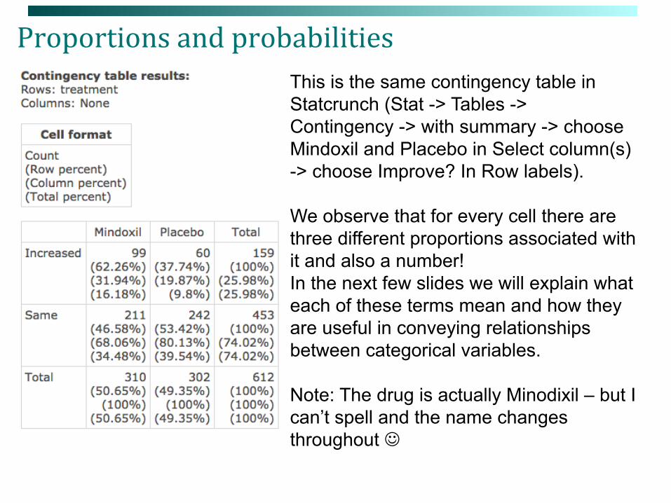
Proportions  and  probabilities  This is the same contingency table in Statcrunch (Stat -> Tables -> Contingency -> with summary -> choose Mindoxil and Placebo in Select column(s) -> choose Improve? In Row labels). We observe that for every cell there are three different proportions associated with it and also a number! In the next few slides we will explain what each of these terms mean and how they are useful in conveying relationships between categorical variables. Note: The drug is actually Minodixil – but I can’t spell and the name changes throughout J

Marginal  probabilities    p  The marginal probability is the chance of an event, but completely

ignores the influence/effect of other factors.

The sum of the proportions always add to one.

Minidoxil placebo Subtotals

Improvement 99 60 159

No improvement 211 242 463

Total 310 302 612

p̂M =

99310 = 0.32 p̂P =

60302 = 0.2 p̂ =

159612 = 0.259

Improvement No Improvement

Proportion pI =

159612 = 0.259 pN =

463612 = (1� 0.259)

Focusing on just hair improvement, we see that 25.9% of the total who received some treatment saw hair improvement, where as 74.1% did not. These probabilities are marginal probabilities, because they do not measure the influence of other variables.

Conditional  probabilities  p  If we want to understand how one variable may influence another, we

need to look at conditional probabilities. Let us return to the Minodixil example. Here we want to understand whether Minodixil increases the chance of hair improvement over the placebo.

To do this we compare the probabilities in two subgroups, the Minodixil group and the Placebo group. Within each group we calculate the proportion that observed an increase in hair growth after taking the designated treatment.

Minidoxil Placebo Subtotals

Improvement 99 60 159

No improvement 211 242 463

Total 310 302 612

We see that 32% percent of the Mindoxil group saw an increase in hair growth, whereas only 20% of Placebo group saw an increase. These are called conditional probabilities, because they are conditional on a treatment.

Minidoxil Placebo Subtotals

Improvement 99 (

99310 = 0.32) 60 (

60302 = 0.2) 159 (

159612 = 0.259)

No improvement 211 (

211310 = 0.68) 242 (

242302 = 0.8) 463 (

463612 = 0.76)

Total 310 302 612

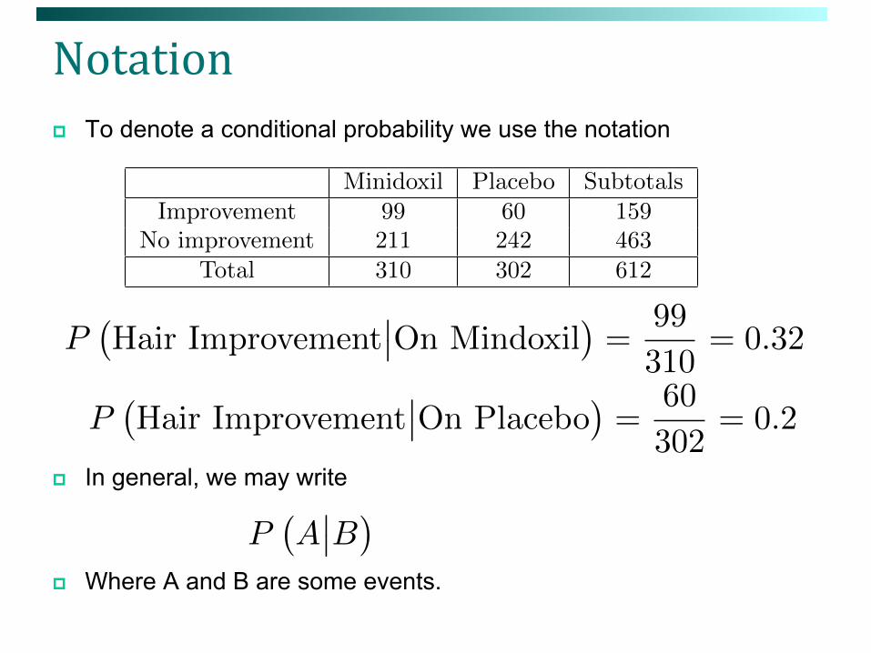
Notation  p  To denote a conditional probability we use the notation

p  In general, we may write

p  Where A and B are some events.

Minidoxil Placebo Subtotals

Improvement 99 60 159

No improvement 211 242 463

Total 310 302 612

P�Hair Improvement

��On Mindoxil�=

99

310= 0.32

P�Hair Improvement

��On Placebo�=

60

302= 0.2

P�A��B

�

Conditional  probabilities  and  independence  p  We recall that in Chapter 12 the focus was on comparing the conditional

probabilities p  By using a two sample test on proportions, Mindoxil increased hair

growth because 32% was `significantly’ larger than 20%. p  What if these two proportions were the same?

p  If the proportions in the Mindoxil and Placebo group were the same it would mean that the treatment did not effect the chance of hair growth (for now we ignore that this is a random sample).

p  Further, if the proportions who saw an increase in the minidoxil group and placebo group were the same, then this would be the same as the marginal probability of an increase (regardless of the treatment given).

p  If this were the case, the treatment used is said to be independent of hair improvement.

p  Two variables are independent if the marginal probabilities and conditional probabilities are the same. p  Put it another way if two variables are independent, then the outcome of one

variable (for example treatment given) is not going to change the chances of another variable (for example hair growth).

p  For the Minidoxil example the data suggests a dependence.

p̂M = 0.32 and p̂P = 0.2

Example  1  (independence):  Gender  and  grades  p  The following pass and fail rate for males and females were observed:

We see that the proportion of males who passed is the same as the proportion of females who passed (90%), which is the same as the overall proportion who passed. This means that at least for this data set, gender does not influence grades. Observations: Do not be fooled by the proportion of passing females (180/320) being greater than the proportion of passing males (108/320). These are joint probabilities, it does not take into account that the number of males and females in the sample are different. This is why we should always compare the conditional probabilities; it takes into account the number in each group.

Male Female Total

Pass 108 (

108120 = 0.9) 180 (

180200 = 0.9) 288 (

288320 = 0.9)

Fail 12 (

12120 = 0.1) 20 (

20200 = 0.1) 32 (

32320 = 0.1)

Total 120 200 320

Example  2  (dependence):  Hair  and  treatment  p  Returning to the Minidoxil/Placebo example:

The conditional probabilities 32% vs 20% (vs the marginal 25.9%) for hair growth are all different, this means that at least for this data set (sample), treatment has an influence on hair growth. Observations: Of course this is only for a sample, to draw any concrete conclusions about the population we have to sure that these differences cannot be explained by random variables. We actually proved that these differences were statistical significant difference in Chapter 12 (and we will do the same thing again in Chapter 14).

Minidoxil Placebo Subtotals

Improvement 99 (

99310 = 0.32) 60 (

60302 = 0.2) 159 (

159612 = 0.259)

No improvement 211 (

211310 = 0.68) 242 (

242302 = 0.8) 463 (

463612 = 0.76)

Total 310 302 612

Example  3  (very  dependent):  Oscar  and  dresses  p  Here we look at what people wore at the Oscars (sample size 420):

The chance a male wears a dress is 0% (in this sample), whereas the chance female wears a dress is 97.7% (in this sample). Observations: In this example we see there is a very strong dependence between gender and whether they wore a dress or not. The chance of a person (regardless of gender) wearing a dress is 215/420 = 51.1%. However, once we know that the person is female the chance shoots up to 97.7%, on the other hand if we know that person is male the chance drops to 0%.

Male Female Total

Dress 0 (

0200 = 0.00) 215 (

215220 = 0.977) 215

No Dress 200 (

200200 = 1) 5 (

5220 = 0.023) 205

Total 200 220 420

Joint  Probabilities  p  A joint probability is the chance of two different events happening

together. Look at the Minidoxil example: Minidoxil Placebo Subtotals

Improvement 99 (

99612 = 0.16) 60 (

60612 = 0.098) 159 (

159612 = 0.259)

No improvement 211 (

211612 = 0.34) 242 (

242612 = 0.395) 463 (

463612 = 0.76)

Total 310 302 612

We see that 16% of the sample took Minidoxil and had hair improvement, whereas 9.8% of the sample took the Placebo and had saw an improvement in hair etc. Donnot get conditional and joint probabilities mixed up. The sum of all the joint probabilities is always one.

Formula for calculating joint probabilities in terms of conditionals and marginals.

P (A and B) = P (A|B)P (B) = P (B|A)P (A)

In the next few slides we illustrate it.

Dependent  events  (examples)  p  What is the chance you will see a person in the middle of campus (on any

given day) is eating an ice-cream? p  If we have no other information about the day. Then this is a marginal

probability. Suppose the marginal probability is 0.2 (20%).

p  Suppose you have information about the day. Today the weather is windy and rainy. With this additional information what is the chance of seeing a person eat an ice-cream? p  When it is rainy and wet, very few people want to eat ice-cream. The chance

drop to 0.01 (1%) p  This is called a conditional probability, because we have reevaluated the

chance based on additional information. We write it as

p  Suppose the weather is warm, what is the chance? p  This is a conditional probability, which we write as

p  Because weather has an influence on ice cream consumption. We say there is a dependence between weather and ice cream.

P�ice cream

��cold weather

�= 0.01

P (ice cream) = 0.2

P�ice cream

��hot weather

�= 0.221

p  If additional information changes the chance of an event, then there is dependence. p  In the previous example, knowledge about the weather changed the

likelihood of seeing a person eating an ice cream. p  The type of therapy a person receive may change of their survival (for

example chemotherapy or operation in the treatment of cancer). p  Gender may have an influence of whether a person wears trousers or a

dress to an occasion. p  If an additional piece of information does not change the chance. This

two events are said to independent. p  For example, the chance of getting an A is 25%. If you know the person is

female and chance remains 25%, then you can say grades and gender are independent events i.e.

p  On the other hand, if you know that person studied 20 hours per week, then it would change the chance of their attaining an A. We conclude that gender does not influence final grade but the amount of hours studied does.

P�Grade A

��Female�= P (Grade A)

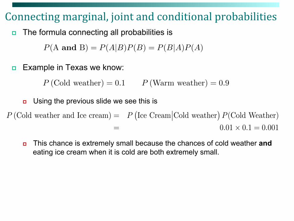
Connecting  marginal,  joint  and  conditional  probabilities      p  The formula connecting all probabilities is

p  Example in Texas we know:

p  Using the previous slide we see this is

p  This chance is extremely small because the chances of cold weather and eating ice cream when it is cold are both extremely small.

P (A and B) = P (A|B)P (B) = P (B|A)P (A)

P (Cold weather) = 0.1 P (Warm weather) = 0.9

P (Cold weather and Ice cream) = P�Ice Cream

��Cold weather

�P (Cold Weather)

= 0.01⇥ 0.1 = 0.001

Example  1:  calculating  joint  probabilities  (minidoxil)  The proportion of people who took minidoxil and saw an improvement is

However, this probability can be calculated in different ways. We know that the proportion who took minidoxil is 50.65% and the proportion of the minidoxil group who saw an improvement is 31.94%, thus the joint probability is their product:

0.1618 = no. who took minidoxil and improved

total number in study

0.1618 = proportion of the minodixil group who saw an improvement

⇥proportion of the sample who took mindoxil

99

310

⇥ 310

612

=

99

612

= P (Minodixol and improved)

Multiplicative  Rule  and  independence  p  We use the notation to denote the proportion of males

who pass (or the probability of passing conditioned on the person being male).

p  In some situations it is not easy to directly calculate this. Instead, if we know the marginal and conditional probabilities we use the multiplicative rule:

q  If there is no association between two variables (or equivalently

they are statistically independent), then the calculation can be written in terms of marginal probabilities. Since

then we have

P (Male and Passed) = P (Passed|male)P (Male)

P (Passed|male)

P (Passed|male) = P (Passed)

P (Male and Passed) = P (Passed|male)⇥ P (Male) = P (Passed)P (Male)

But this probability calculation only holds if passing and gender have no influence on each other. If they do, this calculation is WRONG and can lead to misleading conclusions.

Example  2:  calculating  joint  probabilities  (gender)  To calculate the proportion of students who were males and passed:

Again this probability can be calculated using the marginal and the conditional in tandem:

0.2455 =

108

440

=

males and passed

total

But something interesting happens in this case, the proportion of males who passed is the same as the proportion who passed (independence means the conditional is the same as the marginal) :

0.2455 = proportion of males who passed

⇥proportion of males

108

120

⇥ 120

440

=

108

440

= P (Male and Passed)

0.2455 = proportion who passed

⇥proportion of males

=

396

440

⇥ 120

440

=

108

440

= P (Male and Passed)

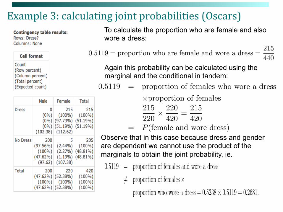
Example  3:  calculating  joint  probabilities  (Oscars)  To calculate the proportion who are female and also wore a dress:

Again this probability can be calculated using the marginal and the conditional in tandem:

Observe that in this case because dress and gender are dependent we cannot use the product of the marginals to obtain the joint probability, ie.

0.5119 = proportion of females who wore a dress

⇥proportion of females

215

220

⇥ 220

420

=

215

420

= P (female and wore dress)

0.5119 = proportion who are female and wore a dress =

215

440

0.5119 = proportion of females and wore a dress

6= proportion of females⇥proportion who wore a dress = 0.5238⇥ 0.5119 = 0.2681.

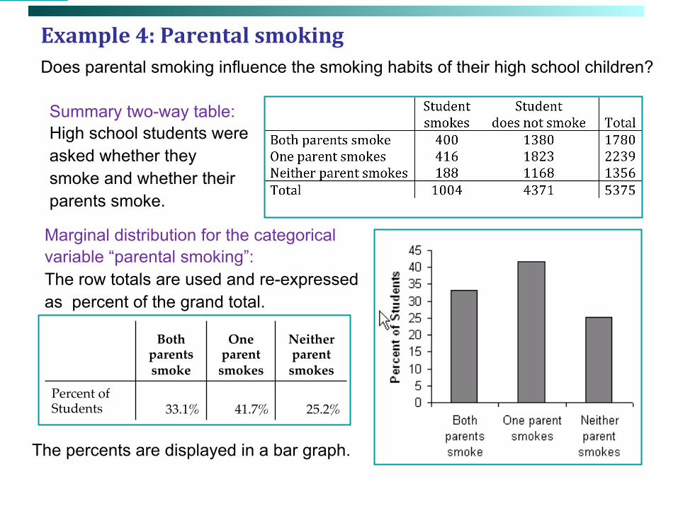
Example  4:  Parental  smoking  Does parental smoking influence the smoking habits of their high school children?

Summary two-way table: High school students were asked whether they smoke and whether their parents smoke.

Marginal distribution for the categorical variable “parental smoking”: The row totals are used and re-expressed as percent of the grand total.

The percents are displayed in a bar graph.

Both parents smoke!

One parent smokes!

Neither parent smokes!

Percent of Students 33.1% 41.7% 25.2%

Comparing the conditional probabilities with the marginal probabilities we see that from this sample there is a 39.84% chance a student smokes if both parents smoke whereas overall there appears to be a 18.68% chance of a student smoking. This difference between the conditional and marginal probabilities means that for this sample there is a dependence between whether a students smokes and whether their parents smoked. In Chapter 14 we use this data to infer dependencies over the entire population of students.

Contingency table results:Rows: ParentColumns: None

Cell format

Count(Row percent)(Column percent)(Total percent)Expected count

Student smokes Does not smoke Total

Both smoke 400(22.47%)(39.84%)(7.442%)

332.5

1380(77.53%)(31.57%)(25.67%)

1448

1780(100.00%)

(33.12%)(33.12%)

One smokes 416(18.58%)(41.43%)

(7.74%)418.2

1823(81.42%)(41.71%)(33.92%)

1821

2239(100.00%)

(41.66%)(41.66%)

None smoke 188(13.86%)(18.73%)(3.498%)

253.3

1168(86.14%)(26.72%)(21.73%)

1103

1356(100.00%)

(25.23%)(25.23%)

Total 1004(18.68%)

(100.00%)(18.68%)

4371(81.32%)

(100.00%)(81.32%)

5375(100.00%)(100.00%)(100.00%)

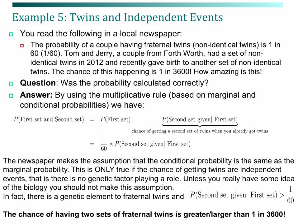
Example  5:  Twins  and  Independent  Events    p  You read the following in a local newspaper:

p  The probability of a couple having fraternal twins (non-identical twins) is 1 in 60 (1/60). Tom and Jerry, a couple from Forth Worth, had a set of non-identical twins in 2012 and recently gave birth to another set of non-identical twins. The chance of this happening is 1 in 3600! How amazing is this!

p  Question: Was the probability calculated correctly? p  Answer: By using the multiplicative rule (based on marginal and

conditional probabilities) we have:

The newspaper makes the assumption that the conditional probability is the same as the marginal probability. This is ONLY true if the chance of getting twins are independent events, that is there is no genetic factor playing a role. Unless you really have some idea of the biology you should not make this assumption. In fact, there is a genetic element to fraternal twins and The chance of having two sets of fraternal twins is greater/larger than 1 in 3600!

P (Second set given| First set) > 1

60

P (First set and Second set) = P (First set) P (Second set given| First set)| {z }chance of getting a second set of twins when you already got twins

=

1

60

⇥ P (Second set given| First set)

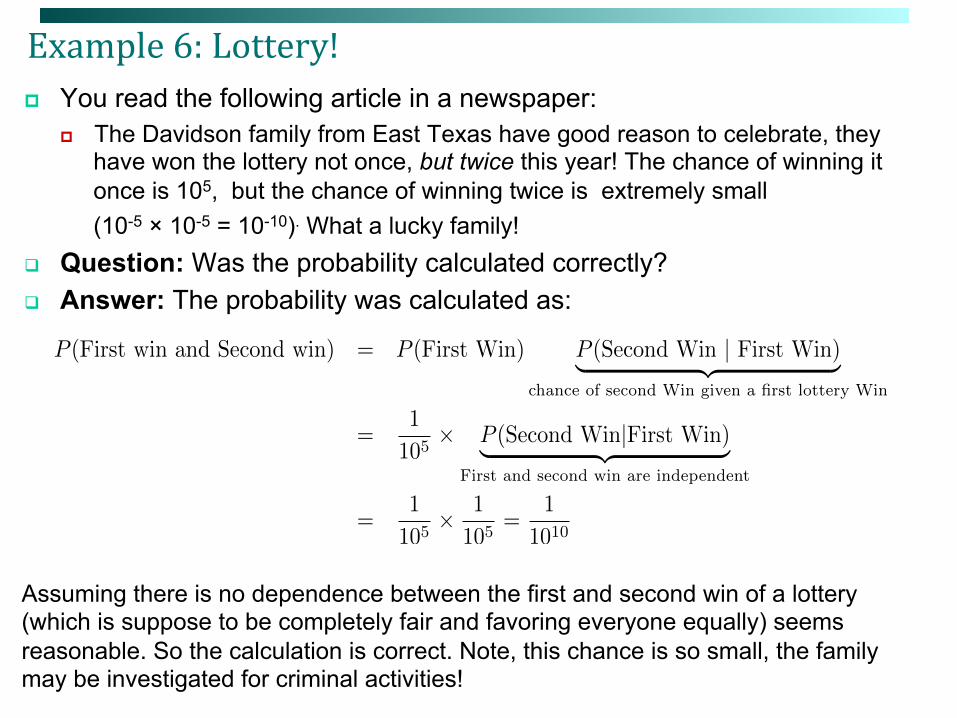
Example  6:  Lottery!  p  You read the following article in a newspaper:

p  The Davidson family from East Texas have good reason to celebrate, they have won the lottery not once, but twice this year! The chance of winning it once is 105, but the chance of winning twice is extremely small

(10-5 × 10-5 = 10-10). What a lucky family! q  Question: Was the probability calculated correctly? q  Answer: The probability was calculated as:

Assuming there is no dependence between the first and second win of a lottery (which is suppose to be completely fair and favoring everyone equally) seems reasonable. So the calculation is correct. Note, this chance is so small, the family may be investigated for criminal activities!

P (First win and Second win) = P (First Win) P (Second Win | First Win)| {z }chance of second Win given a first lottery Win

=

1

10

5

⇥ P (Second Win|First Win)| {z }First and second win are independent

=

1

10

5

⇥ 1

10

5

=

1

10

10

Example  7:  Marathons  p  You read the following article in a newspaper:

p  The Smith family have good reason to celebrate. The Smith Sliblings, Peter and Jane, are both amateur long distance runners and both won the New York Marathon this year! The chance of an amateur winning a major event is 10-3, so the chance that two in the family winning a major event is one in a million

(10-3 × 10-3 = 10-6). What a lucky family! q  Question: Is the calculation correct? q  Answer:

q  The last part of the calculation was based on the assumption that there is no dependence between Peter and Jane winning. Again genetic factors may favor athleticism in a family and it is likely that the chance of Peter winning given that his sister has won is greater than the chance of Peter winning without this additional information ie.

q  It is likely the chance is greater than that calculated.

P (Peter win and Jane win) = P (Peter Win) P (Jane win| Peter Win)| {z }chance of peter winning given that his sister has already won

=1

1000⇥ P (Jane Win| Peter Win)

P (Jane Win| Peter Win) >1

1000

Example  8:  Wrong  calculations    p  There is a tendency that probabilities do not matter. However, it is

important to understand how to calculate probabilities. Wrong calculations can have a terrible effect on peoples lives.

p  The following is a real and rather tragic story of a probability that was not calculated properly.

p  Sally Clark was a successful solicitor http://en.wikipedia.org/wiki/Sally_Clark.

p  In 1996 Sally Clark had her first child, Christopher, who tragically died at less than 3 months old.

p  In 1998 Sally Clark had a second child who also died 8 weeks after being born.

p  After the death of her second child Sally Clark was arrested and charged with the murder of her two children.

p  We will look at the most damning piece of evidence against her, which lead to her conviction, and how this piece of evidence was obtained.

What  the  prosecution  said  p  The most damning piece of evidence against Clark was given by the

pediatrician Prof. Roy Meadows. p  He claimed that for an affluent family like the Clarks, the probability

of a cot death (SIDS – sudden death syndrome) was 1 in 8543, therefore the probability of two cot deaths (this is P(death of first and second child)- so we need to use the multiplicative rule) is 1 in 8543 ×8543 = 1/(73 million) = 1.37×10-8

p  These very small odds, lead to her conviction. p  If we are to write her story as a hypothesis test it is H0: Innocent

against HA: Guilty. p  We shall go through some of the problems with the calculation and

interpretations with this probability. p  The first major problem was with interpretation. The press (in their usual

inability to understand what a probability meant, understood 1 in 73 million as the probability of Sally Clark being innocent). By now, we should understand it has the probability of observing the evidence given that she is innocent. Probability of innocence requires a more sophisticated calculation (and assumptions).

p  The second major problem was the calculation of the probability itself. p  The chance 1 in 8453 that was used is controversial because the general

figure is 1 in 3200. Roy Meadows reduced the odds based on Sally Clark’s affluence, but did not take into account that she had two boys, which increases the odds of a cot death.

p  The most controversial part of his testimony was the calculation of the probability, which gave these tiny odds and was the main reason for Sally Clark’s conviction.

p  In 2001, the Royal Statistical Society wrote a damning report criticizing this calculation. We look at this calculation and it’s fatal flaws.

p  By using the multiplicative rule we have P(First baby dies and Second baby dies) = P(First baby dies)P(Second baby dies|First baby dies) q  We want to calculate this probability under the assumption that they died from

a Cot death. We know over the probability a child dies of a cot death (over the general population) is 1 in 8453, therefore using this

q  P(First baby dies and Second baby dies) = (1/8453)×P(Second baby dies|First baby dies).

p  In order to get the second probability, Roy Meadows assumed that the second probability was equal to its marginal

P (First and Second baby dies) = P (First dies)⇥ P (Second baby dies)|First dies)| {z }P (Second baby dies)

q  We recall that the conditional probability is only equal to its marginal if two variables are independent. This means the probability that the first baby dying it completely independent of the second child dying.

q  However, to make this rather strong assumption we are assuming that the first and second child share not factors in common. But in the case of Sally Clark the two children were brothers.

q  The assumption of statistical independence in this case seems to completely incredulous when applied to siblings!

q  The RSS wrote this in their report, it lead to a second appeal and in 2003 Sally Clark was released.

q  Sadly she never recovered from the experience and died in 2007.

Relationship  between  categorical  variables  The marginal distributions summarize each categorical variable separately. But the two-way table actually provides information about the relationship between the categorical variables.

The cells of a two-way table represent the simultaneous occurrence of a given level of one categorical factor with a given level of the other categorical factor. We can ask whether certain combinations of the variables are generally more (or less) likely to occur together than other combinations.

In the smoking example, we can see that “student smokes” and “neither parent smokes” are relatively unlikely to occur together (even when accounting for the smaller sizes of these groups). More likely are the combinations that “student smokes” and “one or both parents smoke”. We would like to analyze such relationships statistically which we do in Chapter 14.

Association  does  not  mean  cause  p  We have defined the idea of association between two variables, and

in the next section we consider tests. But the associations we see does not necessarily mean that one variable cause the other.

p  These are confounding variables, which we need to investigate in order to come up with causal relationships between two variables.

p  We illustrate this in the next example. p  See IPS, page 519 for more information.

Simpson’s  paradox  An association or comparison that holds for all of several groups can reverse direction when the data are combined (aggregated) to form a single group. This reversal is called Simpson’s paradox.

Hospital A Hospital BDied 63 16Survived 2037 784Total 2100 800% surv. 97.0% 98.0%

All Patients On the surface (from the combined results), Hospital B would seem to have a slightly better record of survival.

Here, Patient Condition is called a “hidden” variable.

Patients in good condition Patients in poor conditionHospital A Hospital B Hospital A Hospital B

Died 6 8 Died 57 8Survived 594 592 Survived 1443 192Total 600 600 Total 1500 200% surv. 99.0% 98.7% % surv. 96.2% 96.0%

But when the patient condition is taken into account, we see that Hospital A admits more patients in a poor condition, which is what gives the appearance of a worse survival record.

Example: Hospital death rates

Accompanying  problems  associated  with  this  Chapter  

p  Quiz 17 p  Homework 9