Abstract — Scanning laser range sensors (ladars) are

frequently used in mobile robotics applications because their

ability to accurately measure the environment in 3D makes

them well-suited for perception tasks like terrain modeling

and obstacle detection. The choice of ladar sensor and the

manner in which it is configured and integrated into a robot

platform is usually determined subjectively based on the

experience of the project team members. This paper develops

a method for evaluating ladar sensors and sensor

configurations that objectively measures the quality of a

sensor/configuration choice in terms of density and uniformity

of measurements within a region of interest. The method is

applicable to static sensors and environments as well as

scenarios with moving objects and mobile sensors. It can be

used to compare different sensors, to evaluate specific sensor

configurations and search for the optimal one, and to aid in

designing new ladar sensors tailored to specific applications.

We find that popular ladar configurations are often not the

best configuration choice, and that alternative configurations

not commonly used would offer better data density and

uniformity.

I. INTRODUCTION

canning laser range sensors (ladars) are frequently used

in mobile robotics applications [1-7]. Ladars provide

accurate 3D measurements of a robot’s environment, which

makes them well-suited for key perception tasks, such as

terrain modeling and obstacle detection. Different ladars

have different properties (e.g., sampling rate, field of view,

angular increment, etc.), and ladar sensors can be mounted

and actuated in a variety of ways. Any project that uses

ladar sensors for perception must make decisions as to

which sensor is to be used and how it is to be configured

during integration. In many projects, these decisions are

made in a subjective manner based on the experience of the

project team members.

This paper presents a method to objectively answer the

questions “Which ladar sensor is the best choice for a given

application?” and “How should a given ladar sensor be

mounted and configured to optimize perception

performance?” Intuitively, since ladars typically operate at a

fixed sampling rate, a ladar configuration that concentrates

This work was supported by the Agency for Defense Development,

Republic of Korea. Thanks also to Lyle Chamberlain for assistance with the

simulation software.

A. Desai is with the Mechanical Engineering Department at Carnegie

Mellon University (CMU), 5000 Forbes Ave., Pittsburgh, PA 15213

(ankit2810@gmail.com).

D. Huber is with the Robotics Institute at CMU (dhuber@cs.cmu.edu).

points in the region of interest for a given application will

be better than one that spreads points uniformly throughout

the environment. For example, if the goal is to model the

terrain for path planning, a configuration in which a large

percentage of the points are uselessly measuring the

distance to the sky is not as good as one that focuses most of

the points on the ground in front of the robot.

Our approach to the problem is to simulate different ladar

configurations and to define an objective measure of data

quality that can be computed for a given configuration (Fig.

1). Armed with an objective data quality measure, it is

possible to compare different ladar sensors to determine

which is better, to search for the optimal configuration for a

given sensor, or to evaluate hypothetical ladar sensor

designs for customizing a sensor for a particular

application.

Our approach focuses on the perception aspects of the

question of ladar quality. We do not consider other factors

unrelated to perception that go into making a decision on

sensor choice or configuration. Some of these factors

include cost, complexity, ease of integration, ruggedness,

and power usage. These factors could be included in a more

complex evaluation metric by combining them with the

perceptual configuration quality measure using appropriate

weighting factors.

II. RELATED WORK

Early work by Kelly characterized scan patterns for

horizontally and vertically nodding ladars analytically but

did not try to objectively compare different configurations

[8]. While analytical formulas for density are easy to

evaluate and manipulate, Kelly’s approach makes numerous

assumptions that are not realistic for laser scanners,

including assumptions that the data is measured

instantaneously, that it is arranged uniformly on a

rectangular grid, and that the laser footprint is the same size

as the range image pixel size. Moreover, the approach does

not have any obvious extension to more complex scanner

configurations. More recently, Wulf and Wagner identified

several additional practical configurations for line scanning

ladars that are rotated using a servo [9]. The authors plotted

scan patterns for these configurations and made subjective

observations about which configuration was most useful for

different robotics and 3D mapping applications. They

observed – as have other researchers – that higher density of

Objective Evaluation of Scanning Ladar

Configurations for Mobile Robots

Ankit Desai and Daniel Huber, Member, IEEE

S

measurements can be obtained by pointing the rotation axis

in the direction of interest [10]. This work, did not consider,

the full space of configurations that we cover, nor did it

include any objective measures to compare the different

configurations. Other scan patterns are possible with

specialized sensors. For example, Blais et al used a lissajous

pattern to improve performance for real-time target tracking

in 3D [11]. They found that lissajous patterns allow

tracking speed that is several orders of magnitude faster

than would be possible with a raster scanning pattern. This

is an example of a scanning configuration that is optimized

for a specific application. Similarly variation of

configurations controlling the degree of data density have

been studied with respect to the domain-specific application

of forest canopy analysis using aerial lidar [12].

III. MODELING LADAR CONFIGURATIONS

Our approach for evaluating ladar configurations utilizes

a ladar simulator to generate point measurements. This

simulator needs to model the basic properties of a sensor,

such as the sampling rate and the laser actuation

mechanism and timing, but it is not necessary to model

advanced properties like data uncertainty, mixed pixels, or

precise laser spot size and shape.

Although a wide variety of ladar sensors are

commercially available, a few technologies and laser

actuation schemes have emerged as the predominant

solutions within the mobile robotics domain. Among the

range measurement technologies, pulsed time of flight

(PTOF) is the dominant technology, though several

amplitude modulated continuous waveform (AMCW)

sensors are available, and flash ladar is a promising next

generation technology. Our approach is general enough to

handle any of these ladar technologies.

A ladar’s actuation scheme determines the pattern of

laser pointing directions over time. One popular approach is

to use a spinning mirror or prism to redirect the laser in a

radial pattern, resulting in a line scanning ladar (e.g., SICK

LMS 200/291 and Hokuyo UTM-30LX). To achieve full 3D

sensing, a second type of actuation is needed. One solution

is to use a servo to mechanically rotate the entire sensor

head, either in a continuous rotation or a back-and-forth

nodding motion. Such sensors are commercially available,

but more frequently they are custom-designed [2-4, 6, 7,

10].

We focus our analysis on this rotating/nodding type of

ladar system, since the design is popular in mobile robotics

applications and presents an interesting array of

configuration parameters that are difficult to manually

optimize. It is straightforward to extend our approach to use

a different ladar simulator in order to analyze other types of

actuation mechanisms, such as that of the Velodyne HDL-

64E S2, which was used in the Urban Grand Challenge [5].

For the rotating/nodding system, we establish three

coordinate frames within the world coordinate system, all

with the same origin located at the scanner center of

projection, but with potentially different orientations (Fig.

2). We denote the axis of the spinning mirror/prism as the

primary rotation axis, and the axis of the rotating/nodding

sensor head as the secondary rotation axis. The world

coordinate frame origin is located at an arbitrary point on

the ground plane with the z axis pointing up with respect to

gravity. The platform coordinate frame is affixed to the

Fig. 1. Overview of our approach. Left: A ladar simulator is used to generate 3D rays. Center: The rays are intersected with surface models, such as the ground

(as shown here) or object models to obtain a distribution of point measurements on the surface. Right: The point measurements are accumulated in a histogram

(log scale), from which data density and uniformity within a region of interest can be evaluated to obtain summary statistics for comparing different ladar

configurations. Here, the ladar is rotated around a vertical axis but is mounted with a 30 degree roll angle.

xS

yS

zS

xP

yP

zP

xH

yH

zH

xW

yW

zW

xW

yW

zW

xW

yW

zW

xS

yS

zS

xP

yP

zP

xH

yH

zH

xW

yW

zW

xW

yW

zW

xW

yW

zW

Fig. 2. We define three coordinate frames within the world coordinate

system (W subscripts). The platform coordinate frame (P subscripts),

which is attached to the vehicle platform, the scanner system coordinate

frame (S subscripts), which is attached to the scanner, and the scanner

head coordinate frame (H subscripts), which nods/rotates with the scan

head.

(potentially moving) platform, with its initial orientation the

same as the world coordinate system. The platform is

oriented so that the x-axis points in the robot’s forward

direction and the y-axis points left. The scanner system

coordinate frame is affixed to the ladar scanner with the z-

axis coincident with the secondary rotation axis. The

scanner head coordinate frame is affixed to the

rotating/nodding portion of the scanner with the z-axis

coincident with the primary rotation axis. Typically, the

primary and secondary axes of the scanner are oriented

orthogonally, but that is not required, and it is not

necessarily the best configuration.

Parameters for a ladar system may be configurable, or

they may be fixed by the choice of the device. The sampling

rate is the number of 3D points that the sensor measures per

second (r). The primary angular increment (∆P) is the angle

between successive samples. The secondary angular

increment (∆S) is the angle that the scanner head rotates

during a single rotation of the spinning mirror. This

parameter is governed by the angular rotation about the

secondary rotation axis. The scanner can have limits on the

field of view in the primary rotation plane (Φline_min,

Φline_max), which are typically not configurable. Several

parameters are associated with how the various coordinate

frames are oriented with respect to one another (Fig. 3). The

pitch angle of the line scan can be adjusted by rotating the

ladar head with respect to the primary rotation axis (ΘP);

the roll angle (ΘR) can be controlled by rotating the sensor

around an axis perpendicular to the primary and secondary

rotation axes; and the secondary rotation axis itself can be

tilted with respect to vertical in the world coordinate frame

(ΘT). Nodding sensors are modeled similarly to rotating

sensors, except that two additional parameters are used to

set the angles where the sensor reverses direction (Φnod_min,

Φnod_max). Finally, the sensor itself can be mounted at a

given height (h) above the ground.

IV. SURFACE MODELS AND REGIONS OF INTEREST

The ladar simulator generates rays emanating from the

ladar, which intersect surfaces in the environment to

produce point measurements. We consider three types of

surface models: a ground surface model, a non-ground

surface model, and an object model (Fig. 4). The ground

surface model is used for analyzing the density and

distribution of points on the ground and is useful, for

example, in terrain modeling. The non-ground surface

model is used for analyzing data distributions on surfaces

above the ground, such as building walls in an indoor

modeling application. The object model is used for

analyzing specific objects that have typical sizes, such as

cars or people, which would be important for an urban

navigation application. Our ground surface model is simply

an infinite horizontal planar surface. We model non-ground

surfaces with a vertical cylindrical surface surrounding the

sensor at a fixed radius R. The object model consists of a set

of vertical rectangular planar surfaces, which can be placed

at arbitrary locations and orientations in the environment.

More complex surface models could be employed for

advanced analysis within this framework. For example, an

actual or simulated terrain surface could be used to analyze

sensor configuration choices for different terrain shapes and

slope characteristics.

Real sensors mounted on real platforms have limited

fields of view due to self-occlusion (e.g., points that hit the

vehicle itself) and sensing range limits. Also, depending on

the application, a specific region may be of importance. For

example, when driving forward, a terrain modeling

algorithm is most interested in the region immediately in

front of the vehicle.

To accommodate these considerations, a region of

interest can be specified, and computations are then limited

to this region. We specify regions of interest on the ground

surface using polar coordinates to limit data to a minimum

and maximum distance from the base of the sensor and a

minimum and maximum azimuth angle in the vehicle

coordinate frame (Fig. 4, left). Regions of interest on non-

ground surfaces are specified in cylindrical coordinates with

a minimum and maximum height and azimuth angle (Fig.

4, right).

In the examples that follow, we use a ground region of

interest with radius 2 to 10 meters and azimuth -60 to 60

degrees in the world coordinate frame. For non-ground

regions, we use a region of interest with height 0 to 3

meters and azimuth -60 to 60 degrees in the world

coordinate frame.

V. EVALUATING LADAR CONFIGURATIONS

In the absence of any domain-specific biases, a good

ΘPΘR

ΘT

Sensor Front

Sensor

Top

Sensor Front

ΘPΘR

ΘT

Sensor Front

Sensor

Top

Sensor Front

Fig. 3. The ladar sensor mounting configuration has three parameters –

the pitch angle (ΘP), the roll angle (ΘR), and the tilt angle (ΘT). See text

for details.

Fig. 4. The three types of surface models – ground (beige plane, left),

non-ground (blue cylinder, right), and objects (red rectangles, left). The

region of interest for ground and non-ground models is shown in orange.

ladar configuration should sense the region of interest as

densely and as uniformly as possible. The advantages of

dense data are obvious, and it is also well-known that

variations in data density can cause difficulties for

algorithms that use such data [13]. We consider time-

independent and time-dependent scenarios separately. The

time-independent scenario is applicable to static scenes with

a non-moving sensor, for example, if a robot periodically

stops and uses the scanning ladar to take a high-resolution

scan of the environment. In this case, a good configuration

should consider point density and uniformity in the spatial

domain, independent of the timing of the sampling. The

time-dependent scenario, on the other hand, is more

appropriate for dynamic scenes or moving sensors. In this

case, a good configuration must optimize the density and

uniformity of sampling in the temporal as well as the spatial

domain. A configuration that works well for the time-

independent scenario is not necessarily optimal for the time-

dependent one, and vice versa.

VI. SPATIAL DATA DISTRIBUTION

The spatial distribution of samples on a surface model

can be visualized using a plot of the data density (Fig. 5).

We compute the data density by quantizing the surface

model into cells and then computing a histogram of the

frequency of laser points falling into each cell, normalizing

by the cell surface area. The ground and object surface

models are quantized into uniform square cells, while the

non-ground surface model is quantized by height and

azimuth, with the azimuth increment chosen to give

approximately square cells for the given radius of the

cylinder. To reduce quantization effects, bilinear

interpolation is used to distribute the contribution of each

sample point into the four cells with centers closest to the

sample point.

While data density is useful for visualization, it is

difficult to compare such plots quantitatively. Therefore, we

compute summary statistics for the region of interest – the

average density (avg

D ) and entropy (E). The average

density is computed using equation (1) and is normalized by

the total number of points sampled (ttl

N ) to eliminate the

effect of different sampling period lengths.

int

avg

int ttl

ND

A N= , (1)

where int

N is the number of points within the interest region

and int

A is the area of the interest region.

Entropy is a common measure of data uniformity, with

higher entropy being more uniformly distributed [14]. The

entropy is computed using Equation (2).

, ,

,

log(1 / )i j i j

i j

E p p=∑ , (2)

where ,i j

p is the fraction of points falling into cell ,i j

C and

i,j iterate over the cells within the region of interest. We use

the convention that when ,i j

p = 0, then 0log(1 / 0) 0= .

One limitation of this approach is that the computations are

somewhat dependent on the choice of cell size. We found

that a cell size of 0.5 m works well for the scale of outdoor

(a) (b) (c)

Fig. 5. Point measurement distributions (top row) and density plots (bottom row, log scale) for different scanning configurations. (a) nodding configuration

using SICK LMS-291 parameters; (b) rotating configuration using LMS-291 parameters; (c) nodding configuration using Hokuyo UTM-30LX parameters.

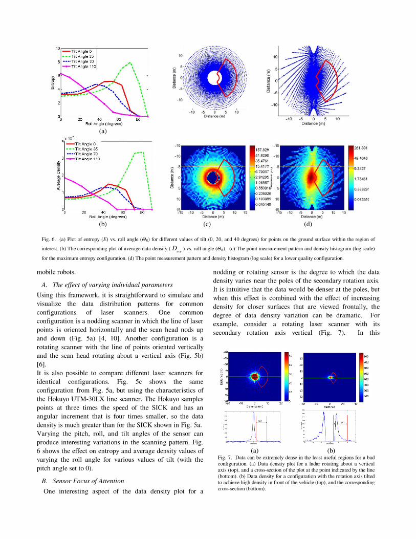
(a) (b) Fig. 7. Data can be extremely dense in the least useful regions for a bad

configuration. (a) Data density plot for a ladar rotating about a vertical

axis (top), and a cross-section of the plot at the point indicated by the line

(bottom). (b) Data density for a configuration with the rotation axis tilted

to achieve high density in front of the vehicle (top), and the corresponding

cross-section (bottom).

mobile robots.

A. The effect of varying individual parameters

Using this framework, it is straightforward to simulate and

visualize the data distribution patterns for common

configurations of laser scanners. One common

configuration is a nodding scanner in which the line of laser

points is oriented horizontally and the scan head nods up

and down (Fig. 5a) [4, 10]. Another configuration is a

rotating scanner with the line of points oriented vertically

and the scan head rotating about a vertical axis (Fig. 5b)

[6].

It is also possible to compare different laser scanners for

identical configurations. Fig. 5c shows the same

configuration from Fig. 5a, but using the characteristics of

the Hokuyo UTM-30LX line scanner. The Hokuyo samples

points at three times the speed of the SICK and has an

angular increment that is four times smaller, so the data

density is much greater than for the SICK shown in Fig. 5a.

Varying the pitch, roll, and tilt angles of the sensor can

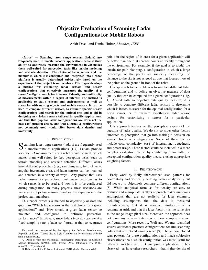
produce interesting variations in the scanning pattern. Fig.

6 shows the effect on entropy and average density values of

varying the roll angle for various values of tilt (with the

pitch angle set to 0).

B. Sensor Focus of Attention

One interesting aspect of the data density plot for a

nodding or rotating sensor is the degree to which the data

density varies near the poles of the secondary rotation axis.

It is intuitive that the data would be denser at the poles, but

when this effect is combined with the effect of increasing

density for closer surfaces that are viewed frontally, the

degree of data density variation can be dramatic. For

example, consider a rotating laser scanner with its

secondary rotation axis vertical (Fig. 7). In this

(a)

(b) (c) (d)

Fig. 6. (a) Plot of entropy (E) vs. roll angle (ΘR) for different values of tilt (0, 20, and 40 degrees) for points on the ground surface within the region of

interest. (b) The corresponding plot of average data density (avg

D ) vs. roll angle (ΘR). (c) The point measurement pattern and density histogram (log scale)

for the maximum entropy configuration. (d) The point measurement pattern and density histogram (log scale) for a lower quality configuration.

Fig. 8. The spatio-temporal entropy plots for a nodding ladar (left) and a

rotating ladar (right).

configuration, the maximum data density on the ground is

over 100 times the density of data 6 meters away from the

sensor. This dense data region occurs directly under the

sensor, which is probably the least useful location to sense

because this region would typically be on the vehicle itself.

Similarly, for a forward-looking nodding sensor, the dense

data regions at the poles are located to the side of the

vehicle, which is not helpful for most tasks.

One alternative is to point the pole of the sensor toward

the direction of interest. This idea has been used by other

researchers in the past, where the secondary axis of a

rotating sensor is pointed straight forward in the direction

of travel [2, 3, 7]. A slight modification of this strategy is to

point the pole slightly downward so that the dense data

region is a fixed distance ahead of the vehicle on the

ground.

The dense data at the poles is analogous to the dense

sensing in the fovea of the human eye. Just as a person uses

focus of attention to gain high resolution data in regions of

importance, a laser scanner could use its polar “foveal”

region more effectively by dynamically pointing it in the

direction of interest. For example, the foveal region could

be constantly focused on a region that is N seconds ahead of

the vehicle, focusing closer when the vehicle slows and

further when it speeds up.

Pointing the axis of rotation at the region of interest does

not necessarily give the highest average density or best

uniformity. Fig. 6a shows that the entropy for tilt angle

110°, which aims the axis of rotation at the center of the

region of interest, gives an entropy of about 6, but an

alternate configuration, with a tilt angle of 35°, gives an

even higher entropy value of over 8. The average density

plots have a similar pattern, but the maximum is at a

slightly different location. These results suggest that the

intuitive notion of pointing the rotation axis at the area of

interest may be too simplistic an approach, and that more

sophisticated pointing strategies could yield denser and

more uniform sensing patterns.

VII. SPATIO-TEMPORAL DATA DISTRIBUTION

When the sensor is on a moving platform, or if the

environment contains moving objects, then the spatial data

distribution measure described above does not capture the

temporal aspect of the data distribution, which can be

misleading for sensor configuration decision-making. For

example, to obtain dense data measurements, one strategy is

to nod/rotate the sensor head very slowly (i.e., choose a

small secondary angular increment). However, the time

between subsequent measurements in one physical location

could be very large in this case. If the sensor or objects in

the environment are moving, this slow nodding/rotation

could lead to significant parts of the environment never

getting imaged at all. Therefore, it is important to consider

the uniformity of measurement distribution across time as

well as space.

Our method for evaluating spatial uniformity can be

extended to incorporate temporal uniformity as well. In this

case, the two dimensional surfaces become quantized three

dimensional volumes, where time is the third dimension.

Measurements are inserted into the volume using trilinear

interpolation, and average density and entropy are

computed over the volume of cuboid cells. The relative size

of the cells in the temporal dimension with respect to the

spatial size of the cells can be used to adjust the balance

between the importance of spatial uniformity and temporal

uniformity, and is a task-specific parameter.

One way to visualize the temporal uniformity of a sensor

configuration is to compute the entropy over time at each

spatial location. At each spatial cell ( ,i jC ), all the cells in

the temporal dimension are used to compute a single

entropy value ( ,i jE ), and the resulting 2D plot of entropy

shows the temporal uniformity across the region of interest.

Fig. 8 shows this type of entropy plot for a nodding and a

rotating sensor. Notice that the entropy for the nodding

configuration is much higher than for the rotating

configuration, since the nodding configuration covers a

much narrower field of view at a faster rate.

A. Effects of Varying Sensor Angular Increment

The primary angular increment is typically fixed by the

sensor choice, but the secondary angular increment is

usually a controllable parameter in nodding/rotating

scanners, since it is directly related to the secondary

rotational velocity. The choice of this parameter can have

significant influence on the spatial or spatio-temporal

uniformity of the data. For a rotating sensor, choosing a

value that is a factor of 360° will result in a data

distribution where the physical location of measurements

repeat with each rotation. While this may be adequate for

moving sensors, when the sensor is not moving, there can

be significant gaps between the measurements, which can

make it hard to detect or track smaller objects. More

concretely, a 10° angular increment results in a 1.75 m gap

between measurements at a distance of 10 m, which could

easily permit missed detections of a person (Fig. 9a). If,

instead, the angular increment is not a factor of 360°, then

the measurement locations will not repeat each time.

One simple way to adjust the angular increment is to

ensure that the measurements repeat only every N rotations.

If the desired angular increment is M, then choosing the

angular increment so that one more (or one less) than the

expected number of measurements occurs in N rotations

will result in a measurement angle that changes by 1/Nth of

the angular increment each rotation. More precisely the new

angular increment M’ should be:

2

(2 / ) 1

NM

N M

π

π′ =

± (3)

One disadvantage of this approach is that the gap

between the initial measurements is filled incrementally, so

that the spatio-temporal distribution of the data is not very

good (Fig. 9b). Ideally, the points would be distributed

uniformly in the temporal domain as well. With a constant

velocity rotation, only a limited amount of uniformity is

possible. If the angular increment is chosen so that

subsequent measurements fall at specific fractions of the

initial angular increment, better spatio-temporal uniformity

can be achieved. Fractional values of 0.6 (3/5), 0.7143

(5/7), and 0.7778 (7/9) give desirable patterns. Equation (4)

can be used for this:

2

2 / 1

fMM

M

π

π

+′ =

+, (4)

where f is the fractional value. For example, if M is 10

degrees and f is 5/7, then M ′ is 9.923 degrees, and the

resulting pattern is shown in Fig. 9c. Our spatio-temporal

uniformity measure shows the benefit of choosing the

angular increment using this strategy, since the entropy

values are much higher in Fig. 9c than in Fig. 9a and b. An

alternative to choosing the angular increment using these

formulas is to search for the best parameter value through

optimization, which is the subject of ongoing work.

B. Modeling Moving Sensors

If the ladar is mounted on a mobile robot, the sensor may

not be stationary. Our approach can also evaluate sensor

configurations on moving platforms. In such cases, we

modify the sensor simulator to model sensor motion. We

have implemented linear motion paths, but the extension to

more complex motion trajectories is straightforward. A

linear motion is accomplished by translating the platform

coordinate frame in a direction l

P with a velocity v

P with

respect to the world coordinate frame.

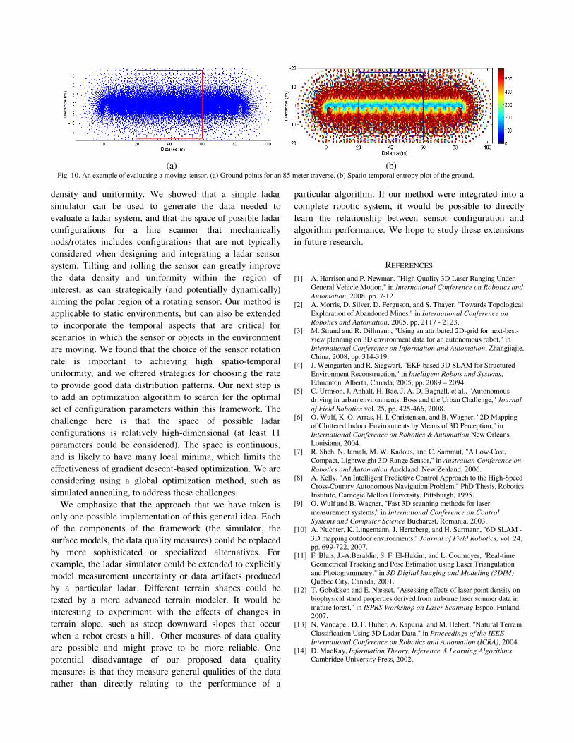
For moving sensors, we limit the analysis to ground

surface and object models. The non-ground cylindrical

surface does not make sense in this situation, because real

objects would not move with the sensor platform. Instead,

we use strategically placed object models to study the effect

of motion on data density and uniformity. Fig. 10 shows an

example of a data density plot for a moving sensor. In this

example, the region of interest is 18 m on either side of the

sensor and covers a fully imaged region along the traverse.

VIII. SUMMARY AND FUTURE DIRECTIONS

We have presented a method for objectively evaluating

ladar sensor configurations. The method considers data

(a) (b) (c)

Fig. 9. Data distribution patterns (top row) and spatio-temporal entropy plots (bottom row) for different choices of angular increment. (a) An even factor of

360 degrees (M = 10 degree) leaves large gaps. (b) Choosing M’ according to equation (3) (M=10, N=5) gives better spatial uniformity, but poor spatio-

temporal uniformity; (c) Choosing M’ according to equation (4) (M=10, f=5/7) gives good spatial and temporal uniformity.

density and uniformity. We showed that a simple ladar

simulator can be used to generate the data needed to

evaluate a ladar system, and that the space of possible ladar

configurations for a line scanner that mechanically

nods/rotates includes configurations that are not typically

considered when designing and integrating a ladar sensor

system. Tilting and rolling the sensor can greatly improve

the data density and uniformity within the region of

interest, as can strategically (and potentially dynamically)

aiming the polar region of a rotating sensor. Our method is

applicable to static environments, but can also be extended

to incorporate the temporal aspects that are critical for

scenarios in which the sensor or objects in the environment

are moving. We found that the choice of the sensor rotation

rate is important to achieving high spatio-temporal

uniformity, and we offered strategies for choosing the rate

to provide good data distribution patterns. Our next step is

to add an optimization algorithm to search for the optimal

set of configuration parameters within this framework. The

challenge here is that the space of possible ladar

configurations is relatively high-dimensional (at least 11

parameters could be considered). The space is continuous,

and is likely to have many local minima, which limits the

effectiveness of gradient descent-based optimization. We are

considering using a global optimization method, such as

simulated annealing, to address these challenges.

We emphasize that the approach that we have taken is

only one possible implementation of this general idea. Each

of the components of the framework (the simulator, the

surface models, the data quality measures) could be replaced

by more sophisticated or specialized alternatives. For

example, the ladar simulator could be extended to explicitly

model measurement uncertainty or data artifacts produced

by a particular ladar. Different terrain shapes could be

tested by a more advanced terrain modeler. It would be

interesting to experiment with the effects of changes in

terrain slope, such as steep downward slopes that occur

when a robot crests a hill. Other measures of data quality

are possible and might prove to be more reliable. One

potential disadvantage of our proposed data quality

measures is that they measure general qualities of the data

rather than directly relating to the performance of a

particular algorithm. If our method were integrated into a

complete robotic system, it would be possible to directly

learn the relationship between sensor configuration and

algorithm performance. We hope to study these extensions

in future research.

REFERENCES

[1] A. Harrison and P. Newman, "High Quality 3D Laser Ranging Under

General Vehicle Motion," in International Conference on Robotics and

Automation, 2008, pp. 7-12.

[2] A. Morris, D. Silver, D. Ferguson, and S. Thayer, "Towards Topological

Exploration of Abandoned Mines," in International Conference on

Robotics and Automation, 2005, pp. 2117 - 2123.

[3] M. Strand and R. Dillmann, "Using an attributed 2D-grid for next-best-

view planning on 3D environment data for an autonomous robot," in

International Conference on Information and Automation, Zhangjiajie,

China, 2008, pp. 314-319.

[4] J. Weingarten and R. Siegwart, "EKF-based 3D SLAM for Structured

Environment Reconstruction," in Intelligent Robots and Systems,

Edmonton, Alberta, Canada, 2005, pp. 2089 – 2094.

[5] C. Urmson, J. Anhalt, H. Bae, J. A. D. Bagnell, et al., "Autonomous

driving in urban environments: Boss and the Urban Challenge," Journal

of Field Robotics vol. 25, pp. 425-466, 2008.

[6] O. Wulf, K. O. Arras, H. I. Christensen, and B. Wagner, "2D Mapping

of Cluttered Indoor Environments by Means of 3D Perception," in

International Conference on Robotics & Automation New Orleans,

Louisiana, 2004.

[7] R. Sheh, N. Jamali, M. W. Kadous, and C. Sammut, "A Low-Cost,

Compact, Lightweight 3D Range Sensor," in Australian Conference on

Robotics and Automation Auckland, New Zealand, 2006.

[8] A. Kelly, "An Intelligent Predictive Control Approach to the High-Speed

Cross-Country Autonomous Navigation Problem," PhD Thesis, Robotics

Institute, Carnegie Mellon University, Pittsburgh, 1995.

[9] O. Wulf and B. Wagner, "Fast 3D scanning methods for laser

measurement systems," in International Conference on Control

Systems and Computer Science Bucharest, Romania, 2003.

[10] A. Nuchter, K. Lingemann, J. Hertzberg, and H. Surmann, "6D SLAM -

3D mapping outdoor environments," Journal of Field Robotics, vol. 24,

pp. 699-722, 2007.

[11] F. Blais, J.-A.Beraldin, S. F. El-Hakim, and L. Coumoyer, "Real-time

Geometrical Tracking and Pose Estimation using Laser Triangulation

and Photogrammetry," in 3D Digital Imaging and Modeling (3DIM)

Québec City, Canada, 2001.

[12] T. Gobakken and E. Næsset, "Assessing effects of laser point density on

biophysical stand properties derived from airborne laser scanner data in

mature forest," in ISPRS Workshop on Laser Scanning Espoo, Finland,

2007.

[13] N. Vandapel, D. F. Huber, A. Kapuria, and M. Hebert, "Natural Terrain

Classification Using 3D Ladar Data," in Proceedings of the IEEE

International Conference on Robotics and Automation (ICRA), 2004.

[14] D. MacKay, Information Theory, Inference & Learning Algorithms:

Cambridge University Press, 2002.

(a) (b) Fig. 10. An example of evaluating a moving sensor. (a) Ground points for an 85 meter traverse. (b) Spatio-temporal entropy plot of the ground.