object perception as bayesian inferenceayuille/pubs/ucla/a189_dkersten_arp2004.pdf · object...

$: Object Perception as Bayesian Inferenceayuille/pubs/ucla/A189_dkersten_ARP2004.pdf · Object Perception as Bayesian Inference ... object shapes, ... also use an \internal generative$
Object Perception as Bayesian Inference 1

Object Perception as Bayesian Inference

Daniel Kersten

Department of Psychology, University of Minnesota

Pascal Mamassian

Department of Psychology, University of Glasgow

Alan Yuille

Departments of Statistics and Psychology, University of California, Los Angeles

KEYWORDS: shape, material, depth, perception, vision, neural, psychophysics, fMRI, com-

puter vision

ABSTRACT:

We perceive the shapes and material properties of objects quickly and reliably despite the

complexity and objective ambiguities of natural images. Typical images are highly complex

because they consist of many objects embedded in background clutter. Moreover, the image

features of an object are extremely variable and ambiguous due to the effects of projection,

occlusion, background clutter, and illumination. The very success of everyday vision implies

neural mechanisms, yet to be understood, that discount irrelevant information and organize

ambiguous or “noisy” local image features into objects and surfaces. Recent work in Bayesian

theories of visual perception has shown how complexity may be managed and ambiguity resolved

through the task-dependent, probabilistic integration of prior object knowledge with image

features.

CONTENTS

OBJECT PERCEPTION: GEOMETRY AND MATERIAL . . . . . . . . . . . . . 2

INTRODUCTION TO BAYES . . . . . . . . . . . . . . . . . . . . . . . . . . . . 3How to resolve ambiguity in object perception? . . . . . . . . . . . . . . . . . . . . . . 3

How does vision deal with the complexity of images? . . . . . . . . . . . . . . . . . . . 5

PSYCHOPHYSICS . . . . . . . . . . . . . . . . . . . . . . . . . . . . . . . . . . . 6Ideal observers . . . . . . . . . . . . . . . . . . . . . . . . . . . . . . . . . . . . . . . . 6

Basic Bayes: The trade-off between feature reliability and priors . . . . . . . . . . . . 7

Discounting & task-dependence . . . . . . . . . . . . . . . . . . . . . . . . . . . . . . . 11

Integration of image measurements & cues . . . . . . . . . . . . . . . . . . . . . . . . 14

Perceptual “explaining away” . . . . . . . . . . . . . . . . . . . . . . . . . . . . . . . . 15

THEORETICAL AND COMPUTATIONAL ADVANCES . . . . . . . . . . . . . 17

Annu. Rev. Psych. 200X 1 1056-8700/97/0610-00

Bayes Decision Theory and Machine Learning. . . . . . . . . . . . . . . . . . . . . . . 17

Learning probability distributions . . . . . . . . . . . . . . . . . . . . . . . . . . . . . . 18

Visual inference . . . . . . . . . . . . . . . . . . . . . . . . . . . . . . . . . . . . . . . . 19

NEURAL IMPLICATIONS . . . . . . . . . . . . . . . . . . . . . . . . . . . . . . 20Network models with lateral connections . . . . . . . . . . . . . . . . . . . . . . . . . . 20

Combining bottom-up and top-down processing . . . . . . . . . . . . . . . . . . . . . . 20

Implementation of the decision rule . . . . . . . . . . . . . . . . . . . . . . . . . . . . . 21

CONCLUSIONS . . . . . . . . . . . . . . . . . . . . . . . . . . . . . . . . . . . . . 22

ACKNOWLEDGMENTS . . . . . . . . . . . . . . . . . . . . . . . . . . . . . . . . 22

LITERATURE CITED . . . . . . . . . . . . . . . . . . . . . . . . . . . . . . . . . 22

1 OBJECT PERCEPTION: GEOMETRY AND MATERIAL

Object perception is important for the everyday activities of recognition, plan-

ning, and motor action. These tasks require the visual system to obtain geo-

metrical information about the shapes of objects, their spatial layout, and their

material properties.

The human visual system is extraordinarily competent at extracting necessary

geometrical information. Navigation, judgments of collision, and reaching rely on

knowledge of spatial relationships between objects, and between the viewer and

object surfaces. Shape-based recognition and actions such as grasping require

information about the internal shapes and boundaries of objects.

Extracting information about the material–the “stuff” that things are made

of–is also important for daily visual function. Image features such as color, tex-

ture, and shading depend on the material reflectivity and roughness of a surface.

Distinguishing different materials is useful for object detection (e.g. texture dif-

ferences are cues for separating figure from ground), as well as for judging affor-

dances such as edibility (e.g. ripe fruit or not) and graspability (e.g. slippery or

not).

Understanding how the brain translates retinal image intensities to useful in-

formation about objects is a tough problem on theoretical grounds alone. The

difficulty of object perception arises because natural images are both complex

and objectively ambiguous. The images received by the eye are complex high-

dimensional functions of scene information (Figure 1). The complexity of the

problem is evident in the primate visual system in which ten million retinal mea-

surements or so are sent to the brain each second, where they are processed by

some billion cortical neurons. The ambiguity of image intensities also poses a

major computational challenge to extracting object information. Similar 3D ge-

ometrical shapes can result in different images, and different shapes can result in

very similar images, Figure 1A & B. Similarly, the same material (e.g. polished

silver) can give rise to drastically different images, depending on the environment,

and the same image can be due to quite different materials, Figure 1C & D.

This paper treats object perception as a visual inference problem (Helmholtz

2


1867) and, more specifically, as statistical inference (Knill & Richards 1996,Ker-

sten 1999,Rao et al 2002). This approach is particularly attractive because it has

been used in computer vision to develop theories and algorithms to extract infor-

mation from natural images useful for recognition and robot actions. Computer

vision has shown how the problems of complexity and ambiguity can be handled

using Bayesian inference, which provides a common framework for modeling ar-

tificial and biological vision. In addition, studies of natural images have shown

statistical regularities that can be used for designing theories of Bayesian infer-

ence. The goal of understanding biological vision also requires using the tools of

psychophysics and neurophysiology to investigate how the visual pathways of the

brain transform image information into percepts and actions.

In the next section, we provide an overview of object perception as Bayesian

inference. In subsequent sections, we review psychophysical (Section 3), compu-

tational, (Section 4) and neurophysiological (Section 5) results on the nature of

the computations and mechanisms that support visual inference. Psychophysi-

cally, a major challenge for vision research is to obtain quantitative models of

human perceptual performance given natural image input for the various func-

tional tasks of vision. These models should be extensible in the sense that one

should be able to build on simple models, rather than having a different model

for each set of psychophysical results. Meeting this challenge will require further

theoretical advances and Section 4 highlights recent progress in learning classi-

fiers, probability distributions, and in visual inference. Psychophysics constrains

neural models, but can only go so far and neural experiments are required to

further determine theories of object perception. Section 5 describes some of the

neural implications of Bayesian theories.

2 INTRODUCTION TO BAYES

2.1 How to resolve ambiguity in object perception?

The Bayesian framework has its origins in Helmholtz’s idea of perception as

“unconscious inference”. Helmholtz realized that retinal images are ambiguous

and that prior knowledge was required to account for perception. For example,

differently curved cylinders can produce exactly the same retinal image if viewed

from the appropriate angles, and the same cylinder can produce very different

images if viewed at different angles. Thus, the ambiguous stimulus in Figure 2A

could be interpreted as a highly curved cylinder from a high angle of view, a

flatter cylinder from a low angle of view, or as concave cylinder from yet another

viewpoint. Helmholtz proposed that the visual system resolves ambiguity through

built-in knowledge of the scene and how retinal images are formed, and uses this

knowledge to automatically and unconsciously infer the properties of objects.

Bayesian statistical decision theory formalizes Helmholtz’s idea of perception

as inference1. Theoretical observers that use Bayesian inference to make opti-

1Recent reviews include Knill et al. (1996), Yuille and Bulthoff (1996), Kersten (2002, 2003),

Maloney (2001), Pizlo (2001), and Mamassian et al. (2002).

4 Kersten et al.

mal interpretations are called ideal observers. Let’s first consider one type of

ideal observer that computes the most probable interpretation given the retinal

image stimulus. Technically, this observer is called a maximum a posteriori or

“MAP” observer. The ideal observer bases its decision on the posterior probabil-

ity distribution–the probability of each possible true state of the scene given the

retinal stimulus. According to Bayes’ theorem, the posterior probability is pro-

portional to the product of the prior probability–the probability of each possible

state of the scene prior to receiving the stimulus, and the likelihood–the proba-

bility of the stimulus given each possible state of the scene. In many applications,

prior probability distributions represent knowledge of the regularities of possible

object shapes, materials, and illumination, and likelihood distributions represent

knowledge of how images are formed through projection onto the retina. Figure 2

illustrates how a symmetric likelihood (a function of the stimulus representing

the curvature of the 2D line) can lead to an asymmetric posterior due to a prior

towards convex objects. The ideal (MAP) observer then picks the most probable

interpretation for that stimulus–i.e. the state of the scene (3D surface curvature

and viewpoint slant) for which the posterior distribution peaks in panel D of

Figure 2. An ideal observer does not necessarily get the right answer for each

input stimulus, but it does make the best guesses so it gets the best performance

averaged over all the stimuli. In this sense an ideal observer may “see” illusions.

Let’s take a closer look at three key aspects to Bayesian modeling: the gener-

ative model, the task specification, and the inference solution.

The generative model. The generative model, S → I, specifies how an image

description I (e.g. the image intensity values or features extracted from them)

is determined by the scene description S (e.g. vector with variables representing

surface shape, material reflectivity, illumination direction, and viewpoint). The

likelihood of the image features, p(I|S), and the prior probability of the scene

description, p(S), determine an external generative model. As illustrated later

in Figure 5, a strong generative model allows one to draw image samples–the

high-dimensional equivalent to throwing a loaded die. The product of the like-

lihood and prior specifies an ensemble distribution p(S, I) = p(I|S)p(S) which

gives a distribution over problem instances, (Section 4). In Bayesian networks,

a generative model specifies the causal relationships between random variables

(e.g. objects, lighting, and viewpoint) that determine the observable data (e.g.

image intensities)2. Below, we describe how Bayesian networks can be used to

cope with the complexity of problems of visual inference.

The task specification. There is a limitation with the MAP ideal observer

described above. Finding the most probable interpretation of the scene does not

allow for the fact that some tasks may require more accurate estimates of some

aspects of the scene than other aspects. For example, it may be critical to get

2When not qualified, we use the term “generative model” to mean an external model that

describes the causal relationship in terms of variables in the scene. Models of inference may

also use an “internal generative model” to test perceptual hypotheses against the incoming data

(e.g. image features). We use the term “strong generative model” to mean one that produces

consistent image samples in terms of intensities.


the exact object shape, but not the exact viewpoint (represented in the utility

function in Figure 2E). The task specifies the costs and benefits associated with

the different possible errors in the perceptual decision. Generally, an optimal

perceptual decision is a function of the task as well as the posterior.

Often we can simplify the task requirements by splitting S into components

(S1, S2) that specify which scene properties are important to estimate (S1, e.g.

surface shape), and which confound the measurements and are not worth esti-

mating at all (S2, e.g. viewpoint, illumination).

The inference solution. Putting things together, Bayesian perception is an in-

verse solution, I → S1, to the generative model, that estimates the variables S1

given the image I and discounts the confounding variables. Decisions are based on

the posterior distribution p(S|I) which, by Bayes, is specified by p(I|S)p(S)/p(I).

The decision may be designed, for example, to choose the scene description for

which the posterior is biggest (MAP). But we’ve noted that other tasks are pos-

sible such as only estimating components of S. In general, an ideal observer

convolves the posterior distribution with a utility function (or negative loss func-

tion)3. The result is the expected utility (or the negative of the expected loss)

associated with each possible interpretation of the stimulus. The Bayes ideal

observer picks the interpretation that has the maximum expected utility (Fig-

ure 2F).

2.2 How does vision deal with the complexity of images?

Recent work (Freeman & Pasztor 1999,Schrater & Kersten 2000,Kersten & Yuille

2003) has shown how specifying generative models in terms of influence graphs

(or “Bayesian networks”, Pearl 1988), together with a description of visual tasks,

allow us to break problems down into categories (see the example in Figure 3A).

The idea is to decompose the description of a scene S into n components S1, . . .,

Sn, the image into m features I1, . . ., Im, and express the ensemble distribution

as p(S1, . . . , Sn; I1, . . . , Im). We represent this distribution by a graph where the

nodes correspond to the variables S1, . . ., Sn and I1, . . ., Im and links are drawn

between nodes which directly influence each other. There is a direct correspon-

dence between graphical structure and the factorization (and thus simplification)

of the joint probability. In the most complex case, every random variable influ-

ences every other one, and the joint probability cannot be factored into simpler

parts. In order to build models for inference, it is useful to first build quantita-

tive models of image formation–external generative models based on real-world

statistics. As we have noted above, the requirements of the task split S into

variables that are important to estimate accurately for the task (disks) and those

which are not (hexagons) (Figure 3B). The consequences of task specification are

described in more detail in subsection 3.3.

In the next Section 3 we review psychophysical results supporting the Bayesian

approach to object perception. The discussion is organized around the four simple

influence graphs of Figure 4.

3Optimists maximize the utility or gain while pessimists minimize their loss.

6 Kersten et al.

3 PSYCHOPHYSICS

Psychophysical experiments test Bayesian theories of human object perception at

several levels. Ideal observers (subsection 3.1) provide the strongest tests, because

they optimally discount and integrate information to achieve a well-defined goal.

But even without an ideal observer model, one can assess the quality of vision’s

built-in knowledge of regularities in the world.

In subsection (3.2) on Basic Bayes, we review the perceptual consequences of

knowledge specified by the prior p(S), the likelihood p(I|S), and the trade-off

between them. Psychophysical experiments can test theories regarding knowl-

edge specified by p(S). For example, the perception of whether a shape is convex

or concave is biased by the assumption that the light source (part of the scene

description S) is above the object. Psychophysics can test theories regarding

knowledge specified by the likelihood, p(I|S). The likelihood characterizes regu-

larities in the image given object properties S, which include effects of projecting

a 3D object onto a 2D image. For example, straight lines in 3D project to straight

lines in the image. Additional image regularities can be obtained by summing

over S to get p(I) =∑

S p(I|S)p(S). These regularities are expected to hold

independently of the specific objects in the scene. Image regularities can be di-

vided into geometric (e.g. bounding contours in the image of an object) and

photometric descriptions (e.g. image texture in a region).

As illustrated in the examples of Figure 3, vision problems have more struc-

ture than Basic Bayes. In subsequent subsections (3.3, 3.4, and 3.5), we review

psychophysical results pertaining to three additional graph categories, each of

which is important for resolving ambiguity: discounting variations to achieve ob-

ject constancy, integration of image measurements for increased reliability, and

perceptual explaining away given competing perceptual hypotheses.

3.1 Ideal observers

Ideal observers provide the strongest psychophysical tests because they are com-

plete models of visual performance based on both the posterior and the task.

A Bayesian ideal observer is designed to maximize a performance measure for

a visual task (e.g. proportion of correct decisions) and as a result serves as a

benchmark with which to compare human performance for the same task (Bar-

low 1962,Green & Swets 1974,Parish & Sperling 1991,Tjan et al 1995,Pelli et al

2003). Characterizing the visual information for a task can be critical for proper

interpretation of psychophysical results (Eckstein et al 2000), as well as for the

analysis of neural information transmission (Geisler & Albrecht 1995,Oram et al

1998).

For example, when deciding whether human object recognition uses 3D shape

cues it is necessary to characterize whether these cues add objectively useful in-

formation for the recognition task (independent of whether the task is being pe-

formed by a person or by a computer). Liu and Kersten (2003) show that human

thresholds for discriminating 3D asymmetric objects is less than for symmetric

objects (the image projections were not symmetric); however, when one compares


human performance to the ideal observer for the task, which takes into account

the redundancy in symmetric objects, human discrimination is more efficient for

symmetric objects.

Because human vision is limited by both the nature of the computations and its

physiological hardware, we might expect significant departures from optimality.

Nevertheless, Bayesian ideal observer models provide a first approximation to

human performance that has been surprisingly effective (cf. Knill 1998, Schrater

& Kersten 2002, Ernst & Banks 2002, Schrater et al 2000).

A major theoretical challenge for ideal observer analysis of human vision is the

requirement for strong generative models so that human observers can be tested

with image samples I drawn from p(I|S). Shortly, we will discuss results from

statistical models of natural image features that constrain, but are not sufficient

to specify the likelihood distribution. Then in Section 4, we discuss relevant work

on machine learning of probability distributions. But let’s first get a preview of

one aspect of the problem.

The need for strong generative models is an extensibility requirement that rules

out classes of models for which the samples are image features. The distinction is

sometimes subtle. The key point is that images features may either be insufficient

to uniquely determine an image or they may sometimes overconstrain it. For ex-

ample, suppose that a system has learned probability models for airplane parts.

Then sampling from these models is highly unlikely to produce an airplane– the

samples will be images, but additional constraints are needed to make sure they

correspond to airplanes, see Figure 5A. Escher’s pictures and other “impossible

figures” such as the impossible trident give examples of images which are not

globally consistent. In addition, local feature responses can sometimes overcon-

strain the image locally. For example, consider the binary image in Figure 5B

and suppose our features ∆L are defined to be the difference in image intensity

L at neighboring pixels. The nature of binary images puts restrictions on the

values that ∆L can take at neighboring pixels. It is impossible, for example,

that neighboring ∆Ls can both take the value +1. So sampling from these fea-

tures will not give a consistent image unless we impose additional constraints.

Additional consistency conditions are also needed in two-dimensional images, see

Figure 5C, where the local image differences in the horizontal, ∆L1,∆L3, and ver-

tical, ∆L2,∆L4, directions must satisfy the constraint ∆L2 +∆L3 = ∆L1 +∆L4

(this is related to the surface integrability condition which must be imposed on

the surface normals of an object to ensure that the surface is consistent).

But it is important to realize that strong generative models can be learned from

measurements of the statistics of feature responses (discussed more in Section 4).

Work by Zhu, Wu, and Mumford (Zhu et al 1997,Zhu 1999) shows how statistics

on image, or shape, features can be used to obtain strong generative models.

Samples from these models are shown in Figure 5D & E.

3.2 Basic Bayes: The trade-off between feature reliability and priors

The objective ambiguity of images arises if several different objects could have

produced the same image description or image features. In this case the visual

8 Kersten et al.

system is forced to guess, but it can make intelligent guesses by biasing its guesses

toward typical objects or interpretations (Sinha & Adelson 1993,Mamassian &

Goutcher 2001,Weiss et al 2002) (see Figure 4A). Bayes formula implies that these

guesses, and hence perception, are a trade-off between image feature reliability,

as embodied by the likelihood p(I|S), and the prior probability p(S). Some

perceptions may be more prior driven, and others more data-driven. The less

reliable the image features (e.g. the more ambiguous), the more the perception is

influenced by the prior. This trade-off has been illustrated for a variety of visual

phenomena (Bulthoff & Yuille 1991,Mamassian & Landy 2001).

In particular, Weiss et al (2002) addressed the “aperture problem” of motion

perception: how to combine locally ambiguous motion measurements into a single

global velocity for an object. The authors constructed a Bayesian model whose

prior is that motions tend to be slow, and which integrates local measurements

according to their reliabilities (see Yuille & Grzywacz 1988 for the same prior

applied to other motion stimuli). With this model (using a single free parameter),

the authors showed that a wide range of motion results in human perception could

be accounted for in terms of the trade-off between the prior and the likelihood.

The Bayesian models give a simple unified explanation for phenomena that had

previously been used to argue for a “bag of tricks” theory requiring many different

mechanisms (Ramachandran 1985).

3.2.1 Prior regularities p(S): Object shape, material, and lighting

Psychophysics can test hypotheses regarding built-in visual knowledge of the prior

p(S) independent of projection and rendering. This can be done at a qualitative

or quantitative level.

Geometry & shape. Some prior regularities refer to the geometry of objects that

humans interact with. For instance, the perception of solid shape is consistently

biased towards convexity rather than concavity (Kanizsa & Gerbino 1976,Hill &

Bruce 1993,Mamassian & Landy 1998,Bertamini2001,Langer & Bulthoff 2001).

This convexity prior is robust over a range of object shapes, sizes and tasks.

More specific tests and ideal observer models will necessitate developing prob-

ability models for the high-dimensional spaces of realistic objects. Some of the

most highly developed work is on human facial surfaces (cf. Vetter & Troje

1997 ). Relating image intensity to such measured surface depth statistics has

yielded computer vision solutions for face recognition (Atick et al 1996) and has

provided objective prior models for face recognition experiments suggesting that

human vision may represent facial characteristics along principal component di-

mensions in an opponent fashion (Leopold et al 2001).

Material. The classical problems of color and lightness constancy are directly

tied to the nature of the materials of objects and environmental lighting. How-

ever, most past work has implicitly or explicitly assumed a special case, that

surfaces are Lambertian (matte). Here, the computer graphics communities have

been instrumental in going beyond the Lambertian model by measuring and char-

acterizing the reflectivities of natural smooth homogeneous surfaces in terms of

the Bidirectional Reflectance Distribution Function (BRDF) (cf. Marschner et al


2000), with important extensions to more complicated textured surfaces (Dana et

al 1999) including human skin (Jensen et al 2001). Real images are of course inti-

mately tied to the structure of illumination, and below we review psychophysical

results on realistic material perception.

Lighting. Studies of human object perception (as well as computer vision) have

traditionally assumed simple lighting models, such as a single point light source

with a directionally non-specific ambient term. One of the best known examples

of a prior is the assumption that light is coming from above. This assumption

is particularly useful to disambiguate convex from concave shapes from shading

information. The light from above prior is natural when one considers that the

sun and most artificial light sources are located above our heads. However, two

different studies have now shown that humans prefer the light source to be located

above-left rather than straight above (Sun & Perona 1998,Mamassian & Goutcher

2001). A convincing explanation for this leftward bias remains to be advanced.

Apparent motion in depth of an object is strongly influenced by the movement

of its cast shadow (Kersten et al 1997, Mamassian et al 1998). This result can

be interpreted in terms of a “stationary light source” prior–the visual system is

more likely to interpret change in the image as being due to a movement of the

object or a change in viewpoint, rather than a movement of the light source.

Do we need more complex lighting models? The answer is surely “yes”, espe-

cially in the context of recent results on the perception of specular surfaces (Flem-

ing et al 2003), and color given indirect lighting (Bloj et al 1999), both discussed

in subsection (3.3). Dror et al (2001) have shown that spatial maps of natural

illumination (Debevec 1998) show statistical regularities similar to those found

in natural images (cf. Simoncelli et al 2001).

3.2.2 Image regularities p(I) =∑

S p(I|S)p(S)

Image regularities arise from the similarity between natural scenes. They cover

geometric properties such as the statistics of edges and photometric properties

such as the distribution of contrast as a function of spatial frequency in the image.

Geometric regularities. Geisler et al. (2001) used spatial filtering to extract lo-

cal edge fragments from natural images. They measured statistics on the distance

between the element centers, the orientation difference between the elements, and

the direction of the second element relative to the orientation of first (reference)

element. A model derived from the measured statistics and from a simple rule

that integrated local contours together could quantitatively predict human con-

tour detection performance. More detailed rules to perceptually organize a chain

of dot elements into a subjective curve with a corner or not, or to be split into one

vs. two groups, have also been given a Bayesian interpretation (Feldman 2001).

Elder & Goldberg (2002) measured statistics of contours from images hand-

segmented into sets of local tangents. These statistics were used to put probabil-

ity distributions on three Gestalt principles of perceptual organization: proxim-

ity, continuation, and luminance similarity. The authors found that these three

grouping cues were independent and that the proximity cue was by far the most

powerful. Moreover, the contour likelihood distribution (the probability of a gap

10 Kersten et al.

length between two tangents of a contour) follows a power law with an exponent

very close to that determined psychophysically on dot lattice experiments.

The work of Geisler et al deals with distributions on image features, namely

edge pairs. To devise a distribution p(I) from which one can draw true contour

samples, one needs to also take into account the consistency condition that edge

pairs have to lie in an image (see Figure 5A for an airplane analogy). Zhu (1999)

learns a distribution on the image itself and thus samples drawn from it produce

contours, see Figure 5E. See also Elder and Goldberg (2002).

Photometric regularities. It is now well-established that natural scenes have

a particular signature in their contrast spatial frequency spectrum in which low

spatial frequencies are over-represented relative to high spatial frequencies. This

regularity is characterized by a 1/f β spectrum, where f is spatial frequency, and

β is a parameter that can be fit from image measurements (Field 1987,Simoncelli

& Olshausen 2001). Human observers are better at discriminating changes in β

for Gaussian and natural images when the values of β are near (Knill et al 1990)

or at the value measured from natural images (Parraga et al 2000), suggesting

that the visual system is in some sense “tuned” to the second-order statistics (i.e.

spatial frequency spectrum) of natural images.

The histograms of spatial filter responses (e.g. the simplest filter being differ-

ences between neighboring pixel intensities) of natural images also show consis-

tent regularities (Olshausen & Field 2000,Simoncelli & Olshausen 2001). The his-

tograms are non-gaussian having a high kurtosis (see first panel in Figure 5C). Zhu

& Mumford (1997) have derived a strong generative model they call a “generic

image prior” based on filter histogram statistics.

3.2.3 Image likelihood p(I|S)

The likelihood characterizes how image regularities result from projection and

rendering of objects as a function of view and lighting, and is related to what is

sometimes called the forward optics or “computer graphics” problem.

Geometrical descriptions. Object perception shows biases consistent with pre-

ferred views. Mamassian & Landy (1998) show how the interpretation of a simple

line drawing figure changed with rotations of the figure about the line of sight.

They modeled their result with a simple Bayesian model that had a prior probabil-

ity for surface normals pointing upward (Figure 2). This prior can be interpreted

as a preference for a viewpoint situated above the scene, which is reasonable when

we consider that most of the objects we interact with are below the line of sight.

Why does a vertical line appear longer than the same line when horizontal?

Although there have been a number of recent studies of the statistics of image

intensities and contours, Howe and Purves (2002) go the next step to directly

compare statistics on the separation between two points in the image with mea-

surements of the causes in the originating 3D scene. The authors found that the

average ratio of the 3D physical interval to the projected image interval from

real-world measurements shows the same pattern as perceived length.

Photometric descriptions. The global spatial frequency amplitude spectrum

is an inadequate statistic to capture the structure of specific texture classes.


More recent work has shown that wavelet representations provide richer models

for category-specific modeling of spatially homogeneous texture regions, such as

“text”, “fur”, “grass”, etc. (Portilla & Simoncelli 2000,Zhu et al 1997). As with

the contour case, a future challenge is to develop strong generative models from

which one can draw samples of images from p(I|S) (Section 4). Promising work

along these lines is illustrated in Figure 5D (Zhu et al 1997).

3.2.4 Where do the priors come from?

Without direct input, how does image-independent knowledge of the world get

built into the visual system? One pat answer is that the priors are in the genes.

Observations of stereotyped periods in the development of human depth percep-

tion do in fact suggest a genetic component (Yonas 2003). In another domain, the

strikingly rapid development of object concepts in children is still a major mys-

tery that suggests predispositions to certain kinds of grouping rules. Adults too

are quick to accurately generalize from a relatively small set of positive examples

(in many domains, including objects) to a whole category. Tenenbaum (1999,

2001) provides a Bayesian synthesis of two theories of generalization (similarity-

like and rule-like), and provides a computational framework that helps to explain

rapid category generalization.

The accurate segmentation of objects such as the kayaks in Figure 1 likely

requires high-level prior knowledge regarding the nature of the forms of possible

object classes. Certain kinds of priors, such as learning the shapes of specific

objects may develop through what Brady and Kersten (2003) have called “op-

portunistic learning” and “bootstrapped learning”. In opportunistic learning, the

visual system seizes the opportunity to learn object structure during those rela-

tively rare occasions when an object is seen under conditions of low ambiguity,

such as when motion breaks camouflage of an object in “plain view”. Boot-

strapped learning operates under low or intermediate conditions of ambiguity

(e.g. in which none of the training images provide a clear view of an object’s

boundaries). Then later, the visual system can apply the prior knowledge gained

to high (objective) ambiguity situations more typical of everyday vision. The

mechanisms of bootstrapped learning are not well-understood although there has

been some computer vision work (Weber et al 2000), see Section 4.

General purpose cortical learning mechanisms have been proposed (Dayan et

al 1995,Hinton & Ghahramani 1997); however, it is not clear whether these are

workable with complex natural image input. We discuss computer vision methods

for learning priors in Section 4.

3.3 Discounting & task-dependence

How does the visual system enable us to infer the same object despite considerable

image variation due to confounding variables such as viewpoint, illumination,

occlusion, and background changes? This is the well-known problem of invariance

or object constancy. Objective ambiguity results when variations in a scene

property change the image description of an object. As we’ve seen, both viewpoint

12 Kersten et al.

and 3D shape influence the 2D image.

Suppose the visual task is to determine object shape, but the presence of un-

known variables (e.g. viewpoint) confounds the inference. Confounding variables

are analogous to “noise” in classical signal detection theory but they are more

complicated to model and they affect image formation in a highly non-linear

manner. For example, a “standard” noise model has I = S + n where n is Gaus-

sian noise. Realistic “vision noise” is better captured by p(I|S) as illustrated in

Figure 6B. Here the problem is making a good guess independent of (or invariant

to) the true value of the confounding variable. The task itself can serve to re-

duce ambiguity by discounting the confounding variable (Freeman 1994,Kersten

1999, Schrater & Kersten 2000,Geisler & Kersten 2002). Discounting irrelevant

scene variations (or accounting for object invariance) has received recent atten-

tion in the fMRI literature where certain cortical areas show more or less degrees

of invariance to size, translation, rotation in depth, or illumination (cf. Grill-

Spector 2003).

From the Bayesian perspective, we can model problems with confounding vari-

ables by the graph in Figure 4B. We define an ensemble distribution p(S1, S2, I),

where S1 is the target (e.g. keys), S2 is the confounding variable (e.g. pose), and

I is the image. Then we discount the confounding variables by integrating them

out (or summing over them):

p(S1, I) =∑

S2

p(S1, S2, I)

This is equivalent to spreading out the loss function completely in one of the

directions (e.g. extending the utility function vertically in Figure 2E). As noted

above, the choice of which variables to discount will depend on the task. View-

point is a confounding variable that can be discounted if the task is to discriminate

objects independent of viewpoint. Illumination is a confounding variable if the

task is to recognize or determine the depth of an object but it is not if the task is

to determine the light source direction. This can be related to notions of utility4,

discounting a variable is equivalent to treating it as having such low utility that

it is not worth estimating (Yuille & Bulthoff 1996), see Section 4.

4Bayesian decision theory, see Section 4, provides a precise language to model the costs of

errors determined by the choice of visual task (Yuille & Bulthoff 1996). The cost or risk R(α; I)

of guessing α when the image measurement is I is defined as the expected loss (or negative

utility):

R(α; I) =∑

S

L(α, S)p(S | I),

with respect to the posterior probability, p(S|I). The best interpretation of the image can then

be made by finding the α which minimizes the risk function. The loss function L(α, S) specifies

the cost of guessing α when the scene variable is S. One possible loss function is −δ(α − S).

In this case the risk becomes R(α; I) = −p(α | I), and then the best strategy is to pick the

most likely interpretation. This is maximum a posteriori (MAP) estimation and is the optimal

strategy for the task requiring an observer to maximize the proportion of correct decisions. A

second kind of loss function assumes that costs are constant over all guesses of a variable. This

is equivalent to “integrating out”, “summing over”, or “marginalization” of the posterior with

respect to that variable.


Viewpoint variation. When interpreting 2D projections of 3D shapes, the hu-

man visual system favors interpretations that assume that the object is being

viewed from a general (or generic) rather than accidental viewpoint (Nakayama

& Shimojo 1992,Albert 2000). Freeman (1994) showed that a Bayesian observer

that integrates out viewpoint can account for the generic view assumption.

How does human vision recognize 3D objects as the same despite changes in

viewpoint? Shape-based object recognition models range between two extremes–

those that predict a strong dependence of recognition performance on viewpoint

(e.g. as a function of familiarity with particular views), and those which as

a result of using view-invariant features together with “structural descriptions”

of objects do not (Poggio & Edelman 1990, Ullman and Basri 1991, Tarr &

Bulthoff 1995, Ullman 1996, Biederman 2000, Riesenhuber & Poggio 2002). By

comparing human performance to several types of ideal observers which integrate

out viewpoint variations, Liu et al. (1995) showed that models that allow rigid

rotations in the image plane of independent 2D templates could not account for

human performance in discriminating novel object views. More recent work by

Liu & Kersten (1998) showed that the performance of human observers relative

to Bayesian affine models (which allow stretching, translations, rotations and

shears in the image) is better for the novel views than for the template views,

suggesting that humans have a better means to generalize to novel views than

could be accomplished with affine warps. Other related work describes the role

of structural knowledge (Liu et al 1999), the importance of view-frequency (Troje

& Kersten 1999), and shape constancy under perspective (Pizlo 1994).

Bayesian task dependence may account for studies where different operational-

isations for measuring perceived depth lead to inconsistent, though related, es-

timates. For instance, the information provided by a single image of an object

is insufficient for an observer to infer a unique shape (see Figure 1B). Not sur-

prisingly, these ambiguities will lead different observers to report different depth

percepts for the same picture, and the same observer to report different per-

cepts when using different depth probes. Koenderink et al. (2001) show that

most of this variability could be accounted for by affine transformations of the

perceived depth, in particular scalings and shears. These affine transformations

correspond to looking at the picture from a different viewpoint. The authors call

the perceived depth of a surface once the viewpoint has been discounted “pictorial

relief”.

Illumination variation. Discounting illumination by integrating it out can re-

duce ambiguity regarding the shape or depth of an object (Freeman 1994,Yuille

et al 2003,Kersten 1999). Integrating out illumination level or direction has also

been used to account for apparent surface color (Brainard & Freeman 1997,Bloj

et al 1999).

Work so far has been for extremely simple lighting, such as a single point light

source. One of the future challenges will be to understand how the visual system

discounts the large spatial variations in natural illumination that are particularly

apparent in many surfaces typically encountered such as metal, plastic, and pa-

per (see Figure 1C). Fleming et al. (2003) showed that human observers could

14 Kersten et al.

match surface reflectance properties more reliably and accurately for more re-

alistic patterns of illumination. They manipulated pixel and wavelet properties

of illumination patterns to show that the visual system’s built-in assumptions

about illumination are of intermediate complexity (e.g. presence of edges and

bright light sources) and rather than depending on high-level knowledge such as

recognizable objects.

3.4 Integration of image measurements & cues

The visual system likely achieves much of its inferential power through sophis-

ticated integration of ambiguous local features. This can be modeled from a

Bayesian perspective (Clark & Yuille 1990). For example, a depth discontinuity

typically causes more than one type of cue (stereo disparity and motion paral-

lax) and visual inference can exploit this to improve the reliability and accuracy

of the depth estimate. Given two conflicting cues to depth, the visual system

might get by with a simple averaging of each estimate, even though inaccurate.

Or in cases of substantial conflict, it may determine that one measurement is

an outlier, and should not be integrated with the other measurement (Landy et

al 1995,Bulthoff & Mallot 1988). Ruling out outliers is possible within a single

modality (e.g. when integrating disparity and texture gradients in vision) but

may not be possible between modalities (e.g. between vision and touch) since in

the latter case, single cue information appears to be preserved (Hillis et al 2002).

The visual system is often more sophisticated and combines image measurements

weighted according to their reliability (Jacobs 2002,Weiss et al 2002) which we

discuss next.

Figure 4C illustrates the influence graph for cue integration with an example

of illumination direction estimation. From a Bayes net perspective, the two

cues are conditionally independent given the shared explanation. An important

case is when the nodes represent Gaussian variables that are independent when

conditioned on the common cause and we have estimates for each cue alone (i.e.

Si is the best estimate of Si from p(S|Ii) ). Then optimal integration (i.e. the

most probable value) of the two estimates takes into account the uncertainty due

to measurement noise (the variance) and is given by the weighted average:

S = S1

r1

r1 + r2

+ S2

r2

r1 + r2

where ri, the reliability, is the reciprocal of the variance. This model has been

used to study whether the human visual system combines cues optimally (cf.

Jacobs 2002 for a review and a discussion of integration in the context of Kalman

filtering, which is a special case of Bayesian estimation).

For instance, visual and haptic information about object size are combined,

weighted according to the reliability of the source (Ernst & Banks 2002,Gepshtein

& Banks 2003). Object size can be perceived both visually and by touch. When

the information from vision and touch disagree, vision usually dominates. The

authors showed that when one takes into account the reliability of the sensory

measurements, information from vision and touch are integrated optimally. Vi-


sual dominance occurs when the reliability of the visual estimation is greater than

that of the haptic one.

Integration is also important for grouping local image elements likely to be-

long to the same surface. The human visual system combines spatial frequency

and orientation information optimally when detecting the boundary between two

regions (Landy & Kojima 2001). Human observers also behave like an opti-

mal observer when integrating information from skew-symmetry and disparity

in perceiving the orientation of a planar object (Saunders & Knill 2001). The

projection of a symmetric flat object has a distorted or skewed symmetry that

provides partial information about the object’s orientation in depth. Saunders

and Knill show that human observers integrate symmetry information with stereo

information weighted according to the reliability of the source.

Prior probabilities can also combine like weighted cues. We saw above that

human observers interpret the shape of an object assuming that both the view-

point and the light source are above the object (Mamassian et al 1998,Mamassian

& Goutcher 2001). Mamassian and Landy (2001) manipulated the reliability of

each of the two constraints by changing the contrast of different parts of the

stimuli. For instance, increasing the shading contrast increased the reliability of

the light source prior and biased the observers’ percept towards the shape most

consistent with the light source prior alone. Their interpretation of the results

was that observers modulated the strength of their priors based on the stimulus

contrast. As a consequence, prior constraints behaved just like depth cue integra-

tion: cues with more reliable information have higher weight attributed to their

corresponding prior constraint.

Not all kinds of cue integrating are consistent with the simple graph of Fig-

ure 4C. Yuille et al. (1996) have argued that strong coupling of visual cues (Clark

& Yuille 1990) is required to model a range of visual phenomena (Bulthoff &

Mallot 1988). The graph for “explaining away” (Figure 4D) provides one useful

simple extension to the graphs discussed so far and we discuss this next.

3.5 Perceptual “explaining away”

The key idea behind explaining away is that two alternative perceptual hypothe-

ses can compete to explain the image. From a Bayesian perspective, the compe-

tition results from the two (otherwise independent) hypotheses becoming condi-

tionally dependent given the image.

Pearl (1988) was one of the first to emphasize that, in contrast to traditional

artificial intelligence expert systems, human reasoning is particularly good at

explaining away the effects of alternative hypotheses. In a now classic example,

imagine that you emerge from your house in the morning and notice that the

grass is wet. Prior probabilities might tell you that it was unlikely due to rain

(e.g. you live in Los Angeles), and thus you’ve probably left the sprinkler on

overnight. But then you check the neighbor’s lawn, and notice that it too is wet.

This auxiliary piece of evidence now undercuts the earlier explanation, and lowers

the probability that you left the sprinkler on. The more probable explanation is

that it rained last night, explaining why both lawns are wet. Both the sprinkler

16 Kersten et al.

and the rain hypothesis directly influence the observation “your lawn is wet”, but

only the rain hypothesis affects both lawns’ being wet.

Human perception is also good at explaining away but automatically and with-

out conscious thought 5. In perception, the essential idea is that if two (or more)

hypotheses about an object property can explain the same image measurements,

then lowering the probability of one of the explanations increases the probability

of the other. One can observe explaining away in both material (e.g. lightness

and color) and shape perception.

Material. In the Land & McCann version of the classic Craik-O’Brien Corn-

sweet illusion, two abutting regions that have the same gradual change of lumi-

nance appear to have different reflectances. Knill and Kersten (1991) found that

the illusion is weakened when a curved occluding contour (auxiliary evidence)

bounding the regions above and below suggests that the variation of luminance

is due to a change a surface orientation, Figure 4D. The lightness gradients are

explained away by the gradual surface curvature. Buckley et al. (1994) extended

this result when binocular disparities were used to suggest a three-dimensional

surface. These results indicate that some scene attributes (in this case surface cur-

vature) influence the inference of the major scene attributes (material reflectance)

that are set by the task.

Another study asked whether human vision could discount the effects of the

color of indirect lighting (Bloj et al 1999). Imagine a concave folded card con-

sisting of a red half facing a white half. With white direct illumination, pinkish

light radiates from the white card because of the indirect additional illumination

from the red card. Does vision use shape knowledge to discount the red illu-

minant in order to perceive the true material color, white? A change in retinal

disparities (an auxiliary measurement) can cause the concave card to appear as

convex, without any change in the chromatic content of the stimulus. When the

card appears convex, the white card appears more pinkish, as if perception has

lost its original explanation for the pinkish tinge in the image and now attributes

it to reddish pigment rather than reddish light.

Geometry & shape. “Explaining away” occurs in discounting the effects of

occlusion, and when simple high-level object descriptions overide more complex

interpretations of line arrangements or moving dots (Lorenceau & Shiffrar 1992,

McDermott et al 2001, Murray et al 2002). We describe this in more detail in

Section 5.

Explaining away is closely related to previous work on competitive models,

where two alternative models compete to explain the same data. It has been

argued that this accounts for a range of visual phenomena (Yuille & Bulthoff 1996)

including the estimation of material properties (Blake & Bulthoff 1990). This

approach has been used successfully in computer vision systems by Tu and Zhu

(2002), including recent work (Tu et al 2003) in which a whole class of generative

models including faces, text, generic shading, and texture models compete and

cooperate to explain the entire image (Section 4). In particular, the generic

5Some related perceptual phenomena Rock described as “perceptual interactions” (Rock

1983).


shading models help detect faces by “explaining away” shadows and glasses.

Failures to explain away. Visual perception can also unexpectedly fail to ex-

plain away. In one simple demonstration, an ambiguous “Mach” folded card can

be interpreted as a concave horizontal edge or a convex vertical edge. A shadow

cast over the edge by an object (e.g. pencil) placed in front provides enough

information to disambiguate the percept, and yet humans fail to use this infor-

mation (Mamassian et al 1998). There has yet to be a good explanation for this

failure.

4 THEORETICAL AND COMPUTATIONAL ADVANCES

Psychophysical and neurophysiological studies of vision necessarily rely on sim-

plifications of both stimuli and tasks. This simplification, however, must be

extensible to the visual input experienced during natural perceptual functioning.

In the previous sections, several psychophysical studies used models of natu-

ral image statistics, as well as models of prior object structure, such as shape.

Future advances in understanding perception will increasingly depend on the

efficient characterization (and simulation) of realistic images to identify informa-

tive image statistics, models of scene properties, and a theoretical understanding

of inference for natural perceptual functions. In this section, we discuss relat-

ing Bayesian decision theory to current theories of machine learning, learning

the probability distributions relevant for vision, and determining algorithms for

Bayesian inference.

4.1 Bayes Decision Theory and Machine Learning.

The Bayesian approach seems completely different from the type of feedforward

models required to recognize objects in 150 milli-seconds (VanRullen & Thorpe

2001). How does the Bayesian approach relate to alternative models based on

neural networks, radial basis functions, or other techniques?

This subsection shows the relationships using concepts from Bayes decision

theory (Berger 1985,Yuille & Bulthoff 1996) and machine learning (Vapnik 1998,

Evgeniou et al 2000, Scholkopf & Smola 2002). This relationship also gives a

justification for Bayes rule and the intuitions behind it.

We first introduce additional concepts from decision theory: (i) a decision

rule S∗ = α(I), and (ii) a loss function (or negative utility) L(α(I), S) which is

the penalty for making the decision α(I) when the true state is S (e.g. a fixed

penalty for a misclassification). Suppose we have a set of examples {Ii, Si : i =

1, ..., N}, then the empirical risk (Vapnik 1998,Scholkopf & Smola 2002) (e.g. the

proportions of misclassifications) of the rule α(I) is defined to be:

Remp(α) = (1/N)N∑

i=1

L(α(Ii), Si). (1)

The best decision rule α∗(.) is selected to minimize Remp(α). For example,

the decision rule is chosen to minimize the number of misclassifications. Neural

18 Kersten et al.

networks and machine learning models select rules to minimize Remp(α) (Vapnik

1998,Evgeniou et al 2000,Scholkopf & Smola 2002).

Now suppose that the samples {Si, Ii} come from a distribution p(S, I) over

the set of problem instances. Then, if we have a sufficient number of samples 6,

we can replace the empirical risk by the true risk:

R(α) =∑

I

∑

S

L(α(I), S)p(S, I). (2)

Minimizing R(α) leads to a decision rule that depends on the posterior dis-

tribution p(S|I) obtained by Bayes rule p(S|I) = p(I|S)p(S)/p(I). To see this,

we rewrite equation (2) as R(α) =∑

I p(I){∑

S p(S|I)L(α(I), S)} where we have

expressed p(S, I) = p(S|I)p(I). So the best decision α(I) for a specify image I is

given by:

α∗(I) = arg minα

∑

S

p(S|I)L(α(I), S), (3)

and depends on the posterior distribution p(S|I). Hence Bayes arises naturally

when you start from the risk function specified by equation (2).

There are two points to be made here. Firstly, the use of the Bayes posterior

p(S|I) follows logically from trying to minimize the number of misclassifications

in the empirical risk (provided there are a sufficient number of samples). Sec-

ondly, it is possible to have an algorithm, or a network, that computes α(.) and

minimizes the Bayes risk but which does not explicitly represent the probability

distributions p(I|S) and p(S). For example, Liu and Kersten (1995) compared

the performance of ideal observers for object recognition with networks using

radial basis functions (Poggio & Girosi 1990). It is possible that the radial basis

networks, given sufficient examples and having sufficient degrees of freedom, are

effectively doing Bayesian inference.

4.2 Learning probability distributions

Recent studies show considerable statistical regularities in natural images and

scene properties that help tame the problems of complexity and ambiguity in ways

that can be exploited by biological, and artificial, visual systems. The theoretical

difficulties of the Bayesian approach reduce to two issues. Firstly, can we learn

the probability distributions p(I|S) and p(S) from real data? Secondly, can we

find algorithms that can compute the best estimators α∗(.)? We briefly review

the advances in learning distributions p(I|S), p(S), p(I), p(S|I) and decision rules

α(I).

The Minimax Entropy theory (Zhu et al 1997) gives a method for learning prob-

ability models for textures p(I|S) where S labels the texture (e.g. cheetah fur).

These models are realistic in the sense that stochastic samples from the models

appear visually similar to the texture examples that the models were trained

on, see Figure 5D. Learning these models is, in principle, similar to determining

6The number of samples required is a complicated issue (Vapnik 1998, Scholkopf & Smola

2002).


the mean and variance of a Gaussian distribution from empirical samples (e.g.

setting the mean of the Gaussian to be the average of the samples from the Gaus-

sian). The input to Minimax Entropy learning are the same histograms of filter

responses that other authors showed were useful for describing textures (Portilla

& Simoncelli 2000). The distribution learned by Minimax Entropy are typically

non-Gaussian but lie in a more general class of distributions called exponential

models. More advanced models of this type can learn distributions with param-

eters representing hidden states (Weber et al 2000).

For certain problems it is also possible to learn the posterior distribution p(S|I)

directly which relates to directly learning a classifier α(I). For example, the

AdaBoost learning algorithm (Freund & Schapire 1999) has been applied very

successfully to build a decision rule α(I) for classfiying between faces (seen from

front-on) and non-faces (Viola & Jones 2001). But the AdaBoost theory shows

that the algorithm can also learn the posterior distributions p(face|I) and p(non-

−face|I) (Hastie et al 2001,Tu et al 2003). Other workers have learned posterior

probabilities p(edge|φ(I)) and p(not − edge|φ(I)) where φ(I) are local image

features (Konishi et al 2003). Similarly Oliva and colleagues have learned a

decision rule α(I) to determine the type of scene (urban, mountain, etc.) from

feature measurements (Oliva & Schyns 2000,Oliva & Torralba 2001). Fine and

Macleod (2003) used the statistics of the spatio-chromatic structure of natural

scenes to segment natural images into regions likely to be part of the same surface.

They computed the probability of whether or not two points within an image fall

on the same surface given measurements of luminance and color differences.

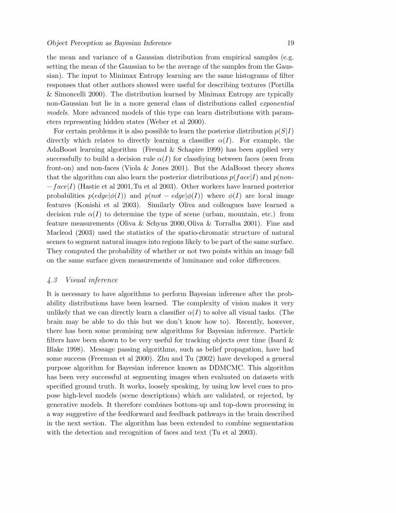
4.3 Visual inference

It is necessary to have algorithms to perform Bayesian inference after the prob-

ability distributions have been learned. The complexity of vision makes it very

unlikely that we can directly learn a classifier α(I) to solve all visual tasks. (The

brain may be able to do this but we don’t know how to). Recently, however,

there has been some promising new algorithms for Bayesian inference. Particle

filters have been shown to be very useful for tracking objects over time (Isard &

Blake 1998). Message passing algorithms, such as belief propagation, have had

some success (Freeman et al 2000). Zhu and Tu (2002) have developed a general

purpose algorithm for Bayesian inference known as DDMCMC. This algorithm

has been very successful at segmenting images when evaluated on datasets with

specified ground truth. It works, loosely speaking, by using low level cues to pro-

pose high-level models (scene descriptions) which are validated, or rejected, by

generative models. It therefore combines bottom-up and top-down processing in

a way suggestive of the feedforward and feedback pathways in the brain described

in the next section. The algorithm has been extended to combine segmentation

with the detection and recognition of faces and text (Tu et al 2003).

20 Kersten et al.

5 NEURAL IMPLICATIONS

What are the neural implications of Bayesian models? The graphical structure

of these models often makes it straightforward to map them onto networks and

suggests neural implementations. The notion of incorporating prior probabilities

in visual inference is frequently associated with top-down biases on decisions.

However, some prior probabilities are likely built into the feedforward processes

through lateral connections. More dramatically, some types of inverse inference

(e.g. to deal with ambiguities of occlusion, rotation in depth, or background clut-

ter) may require an internal generative process that in some sense mirrors aspects

of the external generative model used for inference (Grenander 1996, Mumford

1992,Rao & Ballard 1999,Tu & Zhu 2002a,Tu et al 2003) or for learning (Dayan

et al 1995,Hinton & Ghahramani 1997). There is evidence that descending path-

ways in cortex may be involved in computations that implement model-based

inference using bottom-up and top-down interactions of the sort suggested by

the phenomena of perceptual “explaining away”. In the next two sections, we

discuss Bayesian computations in networks with lateral connections and in larger

scale cortical models that combine bottom-up with top-down information.

5.1 Network models with lateral connections

One class of Bayesian models can be implemented by parallel networks with local

interactions. These include a temporal motion model (Burgi et al 2000) which

was designed to be consistent with neural mechanisms. In this model, the priors

and likelihood functions are implemented by synaptic weights. Another promising

approach is to model the lateral connections within area MT/V5 to account for

the integration and segmentation of image motion (Koechlin et al 1999).

Anatomical constraints will sometimes bias the processing of information in a

way that can be interpreted in terms of prior constraints. For instance, the specific

connections of binocular sensitive cells in primary visual cortex will dictate the

way the visual system solves the correspondence problem for stereopsis. Some

recent psychophysical work suggests that the connections between simple and

complex binocular cells implement a preference for small disparities (Read 2002).

There are also proposed neural mechanisms for representing uncertainty in

neural populations and thereby give a mechanism for weighted cue combination.

The most plausible candidate is population encoding (Pouget et al 2000, Oram

et al 1998,Sanger 1996).

5.2 Combining bottom-up and top-down processing

There is a long history to theories of perception and cognition involving top-

down feedback or “analysis by synthesis” (MacKay 1956). The generative aspect

of Bayesian models is suggestive of the ascending and descending pathways that

connect the visual areas in primates (Bullier 2001,Lamme & Roelfsema 2000,Lee

& Mumford 2003,Zipser et al 1996,Albright & Stoner 2002). The key Bayesian

aspect is model-based fitting, in which models need to compare their predictions


to the image information represented earlier, such as in V1.

A possible role for higher-level visual areas may be to represent hypotheses

regarding object properties, represented for example in the lateral occipital com-

plex (Lerner et al 2001,Grill-Spector et al 2001), that could be used to resolve

ambiguities in the incoming retinal image measurements represented in V1. These

hypotheses could predict incoming data through feedback and be tested by com-

puting a difference signal or residual at the earlier level (Mumford 1992,Rao &

Ballard 1999). Thus, low activity at an early level would mean a “good fit” or

explanation of the image measurements. Experimental support for this possibil-

ity comes from fMRI data (Murray et al 2002, Humphrey et al 1997). Earlier

fMRI work by a number of groups has shown that the human lateral occipital

complex (LOC) has increased activity during object perception. The authors

use fMRI to show that when local visual information is perceptually organized

into whole objects, activity in human primary visual cortex (V1) decreases over

the same period that activity in higher, lateral occipital areas (LOC) increases.

The authors interpret the activity changes in terms of high-level hypotheses that

compete to explain away the incoming sensory data.

There are two alternative theoretical possibilities for why early visual activity

is reduced. High-level areas may explain away the image and cause the early

areas to be completely suppressed–high-level areas tell lower levels to “shut up”.

Such a mechanism would be consistent with the high metabolic cost of neu-

ronal spikes (Lennie 2003). Alternatively, high level areas might sharpen the

responses of the early areas by reducing activity that is inconsistent with the

high level interpretation– high level areas tell lower levels to “stop gossiping”.

The second possibility seems more consistent with some single unit recording

experiments (Lee et al 2002). Lee et al. have shown that cells in V1 and V2 of

macaque monkeys respond to the apparently high-level task of detecting stim-

uli that pop-out due to shape-from-shading. These responses changed with the

animal’s behavioral adaptation to contingencies suggesting dependence on expe-

rience and utility.

Lee and Mumford (2003) review a number of neurophysiological studies consis-

tent with a model of the interactions between cortical areas based on particle filter

methods, which are non-Gaussian extensions of Kalman filters that use Monte

Carlo methods. Their model is consistent with the “stop gossiping” idea. In

other work, Yu & Dayan (2002) raise the intriguing possibility that acetylcholine

levels may be associated with the certainty of top-down information in visual

inference.

5.3 Implementation of the decision rule

One critical component of the Bayesian model is the consideration of the utility

(gain or negative loss in decision theory terminology) associated with each deci-

sion. Where and how is this utility encoded? Platt & Glimcher (1999) systemati-

cally varied the expectation and utility (juice reward) linked to an eye-movement

performed by a monkey. The activity of cells in one area of the parietal cortex was

modulated by the expected reward and the probability that the eye-movement

22 Kersten et al.

will result in a reward. It will be interesting to see whether similar activity

modulations occur within the ventral stream for object recognition decisions.

Gold and Shadlen (Gold & Shadlen 2001) propose neural computations that

can account for categorical decisions about sensory stimuli (e.g. whether a field

of random dots is moving one way or the other) by accumulating information over

time represented by a single quantity representing the logarithm of the likelihood

ratio favoring one alternative over another.

6 CONCLUSIONS

The Bayesian perspective yields a uniform framework for studying object percep-

tion. We have reviewed work that highlights several advantages of this perspec-

tive. First, Bayesian theories explicitly model uncertainty. This is important in

accounting for how the visual system combines large amounts of objectively am-

biguous information to yield percepts that are rarely ambiguous. Second, in the

context of specific experiments, Bayesian theories are optimal, and thus define

ideal observers. Ideal observers characterize visual information for a task and

can thus be critical for interpreting psychophysical and neural results. Third,

Bayesian methods allow the development of quantitative theories at the informa-

tion processing level, avoiding premature commitment to specific neural mech-

anisms. This is closely related to the importance of extensibility in theories.

Bayesian models provide for extensions to more complicated problems involving

natural images and functional tasks as illustrated in recent advances in computer

vision. Fourth, Bayesian theories emphasize the role of the generative model, and

thus tie naturally to the growing body of work on graphical models and Bayesian

networks in other areas such as language, speech, concepts and reasoning. The

generative models also suggest top-down feedback models of information process-

ing in the cortex.

7 ACKNOWLEDGMENTS

Supported by NIH RO1 EY11507-001, EY02587, EY12691 and, EY013875-01A1,

NSF SBR-9631682, 0240148, HFSP RG00109/1999-B and EPSRC GR/R57157/01.

We thank Zili Liu for helpful comments.

8 LITERATURE CITED

Literature Cited

Albert MK. 2000. The generic viewpoint assumption and Bayesian inference. Perception 29:

601-8

Albright TD, & Stoner GR. 2002. Contextual influences on visual processing. Annu Rev Neurosci

25: 339-79

Atick JJ, Griffin PA, & Redlich AN. 1996. Statistical approach to shape from shading: Re-

construction of three-dimensional face surfaces from single two-dimensional images. Neural

Computation 8: 1321-40


Barlow HB. 1962. A method of determining the overall quantum efficiency of visual discrimina-

tions. J. Physiol. (Lond.) 160: 155-68

Berger J. 1985. Statistical Decision Theory and Bayesian Analysis. New York: Springer-Verlag

Bertamini M. 2001. The importance of being convex: An advantage for convexity when judging

position. Perception 30: 1295-310

Biederman I. 2000. Recognizing depth-rotated objects: a review of recent research and theory.

Spat Vis 13: 241-53

Blake A, & Bulthoff HH. 1990. Does the brain know the physics of specular reflection? Nature

343: 165-9

Bloj MG, Kersten D, & Hurlbert AC. 1999. Perception of three-dimensional shape influences

colour perception through mutual illumination. Nature 402: 877-9

Brady MJ, & Kersten D. 2003. Bootstrapped learning of novel objects. Journal of Vision

Brainard DH, & Freeman WT. 1997. Bayesian color constancy. J Opt Soc Am A 14: 1393-411

Buckley D, Frisby JP, & Freeman J. 1994. Lightness perception can be affected by surface

curvature from stereopsis. Perception 23: 869-81

Bullier J. 2001. Integrated model of visual processing. Brain Res Brain Res Rev 36: 96-107

Bulthoff HH, & Mallot HA. 1988. Integration of depth modules: stereo and shading. Journal of

the Optical Society of America, A 5: 1749-58

Bulthoff HH, & Yuille A. 1991. Bayesian models for seeing surfaces and depth. Comments on

Theoretical Biology 2: 283-314

Burgi PY, Yuille AL, & Grzywacz NM. 2000. Probabilistic motion estimation based on temporal

coherence. Neural Comput 12: 1839-67

Clark JJ, & Yuille AL. 1990. Data Fusion for Sensory Information Processing. Boston: Kluwer

Academic Publishers

Dana K, Ginneken Bv, Nayar S, & Koenderink JJ. 1999. Reflectance and texture of real world

surfaces. ACM Transactions on Graphics 18: 1-34

Dayan P, Hinton GE, Neal RM, & Zemel RS. 1995. The Helmholtz machine. Neural Comput 7:

889-904

Debevec PE. 1998. Rendering Synthetic Objects into Real Scenes: Bridging Traditional and

Image-Based Graphics with Global Illumination and High Dynamic Range Photography. Pre-

sented at SIGGRAPH 98

Dror RO, Leung TK, Adelson EH, & Willsky AS. 2001. Statistics of Real-World Illumination.

Presented at Proceedings of CVPR, Hawaii

Eckstein MP, Thomas JP, Palmer J, & Shimozaki SS. 2000. A signal detection model predicts

the effects of set size on visual search accuracy for feature, conjunction, triple conjunction,

and disjunction displays. Percept Psychophys 62: 425-51

Elder JH, & Goldberg RM. 2002. Ecological Statistics of Gestalt Laws for the Perceptual Or-

ganization of Contours. Journal of Vision 2: 324-53

Ernst MO, & Banks MS. 2002. Humans integrate visual and haptic information in a statistically

optimal fashion. Nature 415: 429-33

Evgeniou T, Pontil M, & Poggio T. 2000. Regularization Networks and Support Vector Machines.

Advances in Computational Mathematics 13: 1-50

Feldman J. 2001. Bayesian contour integration. Perception & Psychophysics 63: 1171-82

Field DJ. 1987. Relations between the statistics of natural images and the response properties

of cortical cells. Journal of the Optical Society of America, A 4:2379-94

Fine I, MacLeod DIA, & Boynton GM. 2003. Visual segmentation based on the luminance and

chromaticity statistics of natural scenes. Journal of the Optical Society of America, A Special

Issue on Bayesian and Statistical Approaches to Vision

Fleming RW, Dror RO, & Adelson EH. 2003. Real-world illumination and the perception of

surface reflectance properties. Journal of Vision

Freeman WT. 1994. The generic viewpoint assumption in a framework for visual perception.

Nature 368: 542-5

Freeman WT, & Pasztor EC. 1999. Learning to estimate scenes from images. In Adv. Neural

24 Kersten et al.

Information Processing Systems 11, ed. MS Kearns, SA Solla, & DA Cohn. Cambridge MA:

MIT Press

Freeman WT, Pasztor EC, & Carmichael OT. 2000. Learning low-level vision. Intl. J. Computer

Vision 40: 25-47

Freund Y, & Schapire R. 1999. A short introduction to boosting. Journal of Japanese Society

for Artificial Intelligence 14: 771-80

Geisler WS, & Albrecht DG. 1995. Bayesian analysis of identification performance in monkey

visual cortex: nonlinear mechanisms and stimulus certainty. Vision Res 35: 2723-30

Geisler WS, & Kersten D. 2002. Illusions, perception and Bayes. Nat Neurosci 5: 508-10

Geisler WS, Perry JS, Super BJ, & Gallogly DP. 2001. Edge co-occurrence in natural images

predicts contour grouping performance. Vision Research 41: 711-24

Gepshtein S, & Banks MS. 2003. Viewing geometry determines how vision and haptics combine

in size perception. Curr Biol 13: 483-8

Green DM, & Swets JA. 1974. Signal Detection Theory and Psychophysics. Huntington, New

York: Robert E. Krieger Publishing Company

Gold JI, & Shadlen MN. 2001. Neural computations that underlie decisions about sensory stim-

uli. Trends Cogn Sci 5: 10-6

Grenander U. 1996. Elements of pattern theory. Baltimore: Johns Hopkins University Press

Grill-Spector K, Kourtzi Z, & Kanwisher N. 2001. The lateral occipital complex and its role in

object recognition. Vision Res 41: 1409-22

Grill-Spector K. 2003. The neural basis of object perception. Current Opinion in Neurobiology

13: 1-8

Hastie T. Tibshirani R. , & Friedman J. 2001. The Elements of Statistical Learning. New York:

Springer

Helmholtz H. 1867. Handbuch der physiologischen Optik. Leipzig: L. Voss. (tranlasted in English

by JPC Southall as Treatise on Physiological Optics)

Hill H, & Bruce V. 1993. Independent effects of lighting, orientation, and stereopis on the

hollow-face illusion. Perception 22: 887-97

Hillis JM, Ernst MO, Banks MS, & Landy MS. 2002. Combining sensory information: Manda-

tory fusion within, but not between, senses. Science 298:1627-30

Hinton GE, & Ghahramani Z. 1997. Generative models for discovering sparse distributed rep-

resentations. Philos Trans R Soc Lond B Biol Sci, 352, (1358), 1177-90

Howe CQ, & Purves D. 2002. Range image statistics can explain the anomalous perception of

length. Proc Natl Acad Sci USA 99: 13184-8

Humphrey GK, Goodale MA, Bowen CV, Gati JS, Vilis T, et al. 1997. Differences in perceived

shape from shading correlate with activity in early visual areas. Curr Biol 7: 144-7

Isard M, & Blake A. 1998. Condensation – conditional density propagation for visual tracking.

International Journal of Computer Vision 29: 5-28

Jacobs RA. 2002. What determines visual cue reliability? Trends Cogn Sci 6: 345-50

Jensen HW, Marschner SR, Levoy M, & Hanrahan P. 2001. A practical model for subsurface

light transport. Presented at Computer Graphics (SIGGRAPH)

Kanizsa G, & Gerbino W. 1976. Convexity and symmetry in figure-ground organisation. In

Vision and Artifact, ed. M Henle. New York: Springer

Kersten D. 1999. High-level vision as statistical inference. In The New Cognitive Neurosciences

– 2nd Edition, ed. MS Gazzaniga, pp. 353-63. Cambridge, MA: MIT Press

Kersten D, Mamassian P, & Knill DC. 1997. Moving cast shadows induce apparent motion in

depth. Perception 26: 171-92

Kersten D, & Schrater PW. 2002. Pattern Inference Theory: A Probabilistic Approach to Vision.

In Perception and the Physical World, ed. R Mausfeld, & D Heyer. Chichester: John Wiley

& Sons, Ltd

Kersten D, & Yuille A. 2003. Bayesian models of object perception. Current Opinion in Neuro-

biology 13: 1-9

Knill DC. 1998. Discrimination of planar surface slant from texture: Human and ideal observers


compared. Vision Research 38:1683-711

Knill DC, Field D, & Kersten D. 1990. Human discrimination of fractal images. J Opt Soc Am

A 7: 1113-23

Knill DC, & Kersten D. 1991. Apparent surface curvature affects lightness perception. Nature

351:228-30

Knill DC, Kersten D, & Yuille A. 1996. Introduction: A Bayesian formulation of visual percep-

tion. In Perception as Bayesian Inference, ed. DC Knill & W Richards, pp. 1-21. Cambridge,

UK: Cambridge University Press

Knill DC, & Richards W. 1996. Perception as Bayesian Inference. Cambridge: Cambridge Uni-

versity Press

Koechlin E, Anton JL, & Burnod Y. 1999. Bayesian inference in populations of cortical neurons:

A model of motion integration and segmentation in area MT. Biological Cybernetics 80:25-44

Koenderink JJ, van Doorn AJ, Kappers AM, & Todd JT. 2001. Ambiguity and the ’mental eye’

in pictorial relief. Perception 30: 431-48

Konishi SM, Yuille AL, Coughlan JM, & Zhu SC. 2003, in press. Statistical edge detection:

Learning and evaluating edge cues. Pattern Analysis and Machine Intelligence No. 1, January

2003, pp. 37-48

Lamme VA, & Roelfsema PR. 2000. The distinct modes of vision offered by feedforward and

recurrent processing. Trends Neurosci 23: 571-9

Landy MS, & Kojima H. 2001. Ideal cue combination for localizing texture-defined edges. J Opt

Soc Am A Opt Image Sci Vis 18: 2307-20

Landy MS, Maloney LT, Johnston EB, & Young M. 1995. Measurement and modeling of depth

cue combination: in defense of weak fusion. Vision Res 35: 389-412

Langer MS, & Bulthoff HH. 2001. A prior for global convexity in local shape-from-shading.

Perception 30:403-10

Lee TS, & Mumford D. 2003. Hierarchical Bayesian inference in the visual cortex. Journal of

the Optical Society of America A

Lee TS, Yang CF, Romero RD, & Mumford D. 2002. Neural activity in early visual cortex

reflects behavioral experience and higher-order perceptual saliency. Nat Neurosci 5: 589-97

Legge GE, Hooven TA, Klitz TS, Stephen Mansfield JS, & Tjan BS. 2002. Mr. Chips 2002: new

insights from an ideal-observer model of reading. Vision Res 42: 2219-34

Lennie P. 2003. The cost of cortical computation. Curr Biol 13: 493-7

Leopold DA, O’Toole AJ, Vetter T, & Blanz V. 2001. Prototype-referenced shape encoding

revealed by high-level aftereffects. Nat Neurosci 4: 89-94

Lerner Y, Hendler T, Ben-Bashat D, Harel M, & Malach R. 2001. A hierarchical axis of object

processing stages in the human visual cortex. Cereb Cortex 11: 287-97

Liu Z, & Kersten D. 1998. 2D observers for human 3D object recognition? Vision Res 38:

2507-19

Liu Z, & Kersten D. 2003, in press. 3D symmetric shapes are discriminated more efficiently than

asymmetric ones. Journal of the Optical Society of America A , 20:

Liu Z, Kersten D, & Knill DC. 1999. Stimulus information or internal representation?–a case

study in human object recognition. Vision Research, 39: 603-12

Liu Z, Knill DC, & Kersten D. 1995. Object Classification for Human and Ideal Observers.

Vision Research 35: 549-68

Lorenceau J, & Shiffrar M. 1992. The influence of terminators on motion integration across

space. Vision Res 32: 263-73

MacKay DM. 1956. The epistemological problem for automata. In Automata Studies, ed. CE

Shannon, & J McCarthy, pp. 235-50. Princeton: Princeton University Press

Maloney LT. 2001. Statistical decision theory and biological vision . In Perception and the

Physical World. D. Heyer & R. Mausfeld (Eds). Chichester, UK: Wiley

Mamassian P, & Goutcher R. 2001. Prior knowledge on the illumination position. Cognition 81:

B1-9

Mamassian P, Knill DC, & Kersten D. 1998. The perception of cast shadows. Trends in Cognitive

26 Kersten et al.

Sciences 2: 288-95

Mamassian P, & Landy MS. 1998. Observer biases in the 3D interpretation of line drawings.

Vision Res 38:2817-32

Mamassian P, & Landy MS. 2001. Interaction of visual prior constraints. Vision Res 41: 2653-68

Mamassian P, Landy MS, & Maloney LT. 2002. Bayesian modelling of visual perception. In

Statistical Theories of the Brain. R. Rao, B. Olshausen and M. Lewicki (Eds), pp. 13-36.

Cambridge, MA: MIT Press

Marschner SR, Westin SH, Lafortune PFE, & Torrance KE. 2000. Image-based Measurement

of the Bidirectional Reflectance Distribution Function. Applied Optics 39

McDermott J, Weiss Y, & Adelson EH. 2001. Beyond junctions: nonlocal form constraints on

motion interpretation. Perception 30: 905-23

Mumford D. 1992. On the computational architecture of the neocortex. II. The role of cortico-

cortical loops. Biol Cybern 66: 241-51

Murray SO, Kersten D, Olshausen BA, Schrater P, & Woods DL. 2002. Shape perception reduces

activity in human primary visual cortex. Proc Natl Acad Sci USA 99: 15164-9

Nakayama K, & Shimojo S. 1992. Experiencing and perceiving visual surfaces. Science 257:

1357-63

Oliva A, & Schyns PG. 2000. Diagnostic colors mediate scene recognition. Cognit Psychol 41:

176-210

Oliva A, & Torralba A. 2001. Modeling the shape of the scene: A holistic representation of the

spatial envelope. International Journal of Computer Vision 42:145-75

Oram MW, Foldiak P, Perrett DI, & Sengpiel F. 1998. The ’Ideal Homunculus’: decoding neural

population signals. Trends Neurosci 21: 259-65

Olshausen BA, & Field DJ. 2000. Vision and the Coding of Natural Images. American Scientist

88: 238-45

Parish DH, & Sperling G. 1991. Object spatial frequencies, retinal spatial frequencies, noise,

and the efficiency of letter discrimination. Vision Res 31: 1399-415

Parraga CA, Troscianko T, & Tolhurst DJ. 2000. The human visual system is optimised for

processing the spatial information in natural visual images. Current Biology 10:35-8

Pearl J. 1988. Probabilistic Reasoning in Intelligent Systems: Networks of Plausible Inference.

San Mateo, Calif.: Morgan Kaufmann Publishers

Pelli DG, Farell B, & Moore DC. 2003. The remarkable inefficiency of word recognition. Nature

Pizlo Z. 1994. A Theory of Shape Constancy Based on Perspective Invariants. Vision Research

34: 1637-58

Pizlo Z. 2001. Perception viewed as an inverse problem. Vision Research 41:3145-61

Platt ML, & Glimcher PW. 1999. Neural correlates of decision variables in parietal cortex.

Nature 400: 233-8

Poggio T, & Edelman S. 1990. A network that learns to recognize three-dimensional objects.

Nature 343: 263-6

Poggio T, & Girosi F. 1990. Regularization algorithms for learning that are equivalent to mul-

tilayer networks. Science 247: 978-82

Portilla J, & Simoncelli EP. 2000. A parametric texture model based on joint statistics of complex

wavelet coefficients. Int’l Journal of Computer Vision 40: 9-71

Pouget A, Dayan P, & Zemel R. 2000. Information processing with population codes. Nat Rev

Neurosci 1: 125-32

Ramachandran VS. 1985. The neurobiology of perception. Perception 14: 97-103

Rao RP, & Ballard DH. 1999. Predictive coding in the visual cortex: a functional interpretation

of some extra-classical receptive-field effects [see comments]. Nat Neurosci 2: 79-87

Rao RPN, Olshausen BA, & Lewicki MS. 2002. Probabilistic models of the brain : perception

and neural function edited by Rajesh P.N. Rao, Bruno A. Olshausen, Michael S. Lewicki.

Cambridge, Mass.: MIT Press

Read JCA. 2002. A Bayesian model of stereopsis depth and motion direction discrimination.

Biological Cybernetics 86: 117-36


Riesenhuber M, & Poggio T. 2002. Neural mechanisms of object recognition. Curr Opin Neu-

robiol 12: 162-8

Rock I. 1983. The Logic of Perception. Cambridge, Massachusetts: MIT Press

Sanger TD. 1996. Probability density estimation for the interpretation of neural population

codes. Journal of Neurophysiology 76: 2790-3

Saunders JA, & Knill DC. 2001. Perception of 3D surface orientation from skew symmetry.

Vision Res 41: 3163-83

Schrater PR, & Kersten D. 2000. How optimal depth cue integration depends on the task.

International Journal of Computer Vision 40: 73-91

Schrater PR, & Kersten D. 2002. Vision, Psychophysics, and Bayes. In Statistical Theories of

the Brain. R. Rao, B. Olshausen and M. Lewicki, MIT press

Schrater PR, Knill DC, & Simoncelli EP. 2000. Mechanisms of visual motion detection. Nature

Neuroscience 1: 64-8

Scholkopf B, & Smola AJ. 2002. Learning with Kernels: Support Vector Machines, Regulariza-

tion, Optimization, and beyond. Cambridge, Mass.: MIT Press

Simoncelli EP, & Olshausen BA. 2001. Natural image statistics and neural representation. Annu

Rev Neurosci 24: 1193-216

Sinha P, & Adelson E. 1993. Recovering reflectance and illumination in a world of painted

polyhedra. Presented at Proceedings of Fourth International Conference on Computer Vision,

Berlin

Sun J, & Perona P. 1998. Where is the sun? Nature Neuroscience 1:183-4

Tarr MJ, & Bulthoff HH. 1995. Is human object recognition better described by geon structural

descriptions or by multiple views? Comment on Biederman and Gerhardstein (1993). J Exp

Psychol Hum Percept Perform 21: 1494-505

Tenenbaum JB. 1999. Bayesian modeling of human concept learning. Presented at Advances in

Neural Information Processing Systems

Tenenbaum JB, & Griffiths TL. 2001. Generalization, similarity, and Bayesian inference. Behav

Brain Sci 24: 629-40; discussion 652-791

Tjan BS, Braje WL, Legge GE, & Kersten D. 1995. Human efficiency for recognizing 3-D objects

in luminance noise. Vision Res 35: 3053-69

Troje NF, & Kersten D. 1999. Viewpoint dependent recognition of familiar faces. Perception 28:

483-7

Tu Z, & Zhu S-C. 2002. Image Segmentation by Data-Driven Markov Chain Monte Carlo. IEEE

Trans. on Pattern Analysis and Machine Intelligence 24

Tu Z, & Zhu S-C. 2002. Parsing Images into Region and Curve Processes. Presented at Proc. of

the 7th European Conference on Computer Vision

Tu Z, Chen A, Yuille AL, & Zhu SC. 2003. Image Parsing. Proceedings of International Confer-

ence on Computer Vision. ICCV’2003. Cannes. France.

Ullman S. & Basri R. 1991. Recognition by linear combination of models. IEEE Trans. Pattern

Analysis and Machine Intelligence 13: 992–1006

Ullman S. 1996. High-level Vision: Object Recognition and Visual Cognition. Cambridge, Mas-

sachusetts: MIT Press

Vapnik VN. 1998. Statistical learning theory. New York: Wiley

VanRullen R, & Thorpe SJ. 2001. Is it a bird? Is it a plane? Ultra-rapid visual categorisation

of natural and artifactual objects. Perception 30: 655-68

Vetter T, & Troje NF. 1997. Separation of texture and shape in images of faces for image coding

and synthesis. Journal of the Optical Society of America A 14: 2152-61

Viola P, & Jones MJ. 2001. Robust real-time object detection. Proc. of IEEE Workshop on

Statistical and Computational Theories of Vision

Weber M, Welling M, & Perona P. 2000. Unsupervised Learning of Models for Recognition.

Presented at Proc. ECCV, Proc. 6th Europ. Conf. Comp. Vis., Dublin, Ireland

Weiss Y, Simoncelli EP, & Adelson EH. 2002. Motion illusions as optimal percepts. Nat Neurosci

5: 598-604

28 Kersten et al.

Yonas A, ed. in press. Development of space perception. In Encyclopedia of Cognitive Science,

ed. R Anand, pp. 96-100. London, England: Macmillan Publishers Ltd

Yu AJ, & Dayan P. 2002. Acetylcholine in cortical inference. Neural Netw 15: 719-30

Yuille AL, & Bulthoff HH. 1996. Bayesian decision theory and psychophysics. In Perception as

Bayesian Inference, ed. DC Knill & W Richards, pp. 123-161. Cambridge, UK: Cambridge

University Press

Yuille AL, Coughlan JM, & Konishi S. 2001. The KGBR Viewpoint-Lighting Ambiguity and its

Resolution by Generic Constraints. Presented at Proceedings ICCV’01, Vancouver, Canada

Yuille A, Coughlan JM, & Konishi S. 2003. The KGBR viewpoint-lighting ambiguity. J Opt Soc

Am A Opt Image Sci Vis 20: 24-31

Yuille A, & Grzywacz N. 1988. A computational theory for the perception of coherent visual

motion. Nature 333: 71-4

Zhu SC, & Mumford D. 1997. Prior Learning and Gibbs Reaction-Diffusion. IEEE Trans. on

PAMI 19: 1236-50

Zhu SC, Wu Y, & Mumford D. 1997. Minimax Entropy Principle and Its Applications to Texture

Modeling. Neural Computation 9: 1627-60

Zhu SC. 1999. Embedding Gestalt Laws in Markov Random Fields. IEEE Trans. Pattern Anal-

ysis and Machine Intelligence. 21

Zipser K, Lamme VA, & Schiller PH. 1996. Contextual modulation in primary visual cortex. J

Neurosci 16: 7376-89


A. B.

C. D.

Figure 1: Visual complexity and ambiguity. A. The same object, a kayak, can

produce different images. The plots below the images show surface plots of the

intensity as a function of position illustrating the complex variations typical of

natural image data that result from a change in view and environment. B. Differ-

ent shapes (three-quarter views of two different facial surfaces in the top panel)

can produce the same image (frontal view of the two faces in the bottom panel)

with an appropriate change of illumination direction. C. The same material can

produce different images. A shiny silver pot reflects completely different patterns

depending on its illumination environment. D. Different materials can produce

the same images. The image of a silver pot could be the result of paint (right-

most panel). The silver pot renderings were produced by Bruce Hartung using

illumination maps made available at: www.debevec.org/Probes/. (Debevec 1998)

30 Kersten et al.

-1/R 0 1/R-π/2

-π/4

0

π/4

π/2Likelihood Function

Surface Curvature

Su

rfa

ce

Sla

nt

Prior Probability

Surface Curvature

Su

rfa

ce

Sla

nt

Posterior Probability

Surface Curvature

Su

rfa

ce

Sla

nt

Utility Function

Curvature Error

Sla

nt

Err

or

Expected Utility

Surface Curvature

Su

rfa

ce

Sla

nt

-1/R 0 1/R-π/2

-π/4

0

π/4

π/2

-1/R 0 1/R-π/2

-π/4

0

π/4

π/2

-1/R 0 1/R-π/2

-π/4

0

π/4

π/2

-1/R 0 1/R-π/2

-π/4

0

π/4

π/2

cvxccv

cvxccv cvxccv

cvxccv

image

–

+

cvx

+

cvx

ccv

A

B

C D

E F

Figure 2: The ideal observer. A. The image of a cylinder is consistent with mul-

tiple objects and viewpoints, including convex cylinders viewed from above and

concave cylinders viewed from below. Therefore, different scene interpretations

for this image vary in the estimated surface curvature and slant (the viewing

angle). B. The likelihood represents the compatibility of different scene interpre-

tations with the image (1/R is the curvature in the image). The hatched region

represents those surface curvatures that are never compatible with the image,

indicating that for instance a plane will never project as a curved patch in the

image. C. The prior probability describes here an observer preference for convex

objects viewed from above. D. A Bayesian observer then combines likelihood

and prior to estimate a posterior probability for each interpretation given the

original image. The maximum a posteriori (MAP) is the set of scene parameters

for which the posterior is the largest. E. The utility function represents the costs

associated to errors in the estimation of the surface slant and curvature and is

dependent on the task. F. Finally, the posterior probability is convolved with the

utility function to give the expected utility associated with each interpretation.


A. B.Scene

Local imagefeatures

Globalfeatures

Haptic

Object class

Objectreflectivity

Objectshape

Environment

Scene

Local imagefeatures

Globalfeatures

Haptic

Object class

Objectreflectivity

Objectshape

Environment

S1

S2

S5S4

S3

I1 I2 I3

Imagemeasurement

Auxilarymeasurement

Accurate sceneestimate needed

Rough sceneestimate sufficient

Figure 3: Infuence graphs and the visual task. A. An example of an influence

graph. Arrows indicate causal links between nodes that represent random vari-

ables. The scene class (indoor or outdoor) influences the kind of illumination

and background that determine the environment. The scene also determines the

kinds of objects one may find (artifactual or not). Object reflectivity (“paint”

or pigment) and shape are influenced by the object class. The model of lighting

specified by the environment interacts with reflectivity and shape to determine

the image measurements or features. The environment can determine large-scale

global features (e.g. overall contrast and color, spatial frequency spectrum) that

may be relatively unaffected by smaller scale objects of interest. Global features

can serve to set a context. B. The inference problem depends on the task. The

task specifies which variables are important to estimate accurately (disks), which

are not (hexagons). Triangles represent image measurements or features. For the

purpose of later illustration of “explaining away”, we also distinguish auxiliary

features (upside-down triangles) that are available or actively sought and which

can modulate the probability of object variables that do not directly influence the

auxiliary variable itself. Note that perceptual inference goes against the arrows.

32 Kersten et al.

A. Basic Bayes B. Discounting

C. Cue Integration D. "Explaining Away"

S1: Reflectance S2: 3D Shape

I1: Shading I2: Contour

oror

S1

I1

I2

S1: 3D Shape

I1: 2D Image

I1: Shading I2: Shadow

S1: Illumination

or S1: Keys S2: Pose

I1: Image

Figure 4: Four simple categories of influence graphs. A. Basic Bayes. The four

curved line segments are consistent with both a spherical and saddle-shaped sur-

face patch (and an infinite family of other 3D interpretations). Human observers

prefer the convex spherical interpretation (Mamassian & Landy 1998). B. Dis-

counting. A given object or object class can give rise to an infinite variety of

images because of variations introduced by confounding variables such as pose,

viewpoint, illumination, and background clutter. Robust object recognition re-

quires some degree of object invariance or constancy requiring vision to discount

confounding variables such as pose illustrated here. There is a one to one relation-

ship between graph structure and factorizing the joint probability. If Ii and Sj

indicate the ith image and jth object variables respectively, then p(..., Sj ..., Ii, ...)

is the joint probability. For this graph, p(S1, S2, I) = p(I|S1, S2)p(S1)p(S2). C.

Cue integration. A single cause in a scene can give rise to more than one effect

in the image. Illumination position affects both the shading on the ball, and the

relationship between the ball and shadow positions in the image. Both kinds of

image measurement can in principle be combined to yield a more reliable esti-

mate of illumination direction than either alone, and it is an empirical question

to find out if human vision combines such cues, and if so, how optimally. For this

graph, p(S1, I1, I2) = p(I1|S1)p(I2|S1)p(S1). D. Explaining away. An image mea-

surement (ambiguous horizontal shading gradients) can be caused by a change in

reflectance or a change in 3D shape. A change in the probability of one of them

being the true cause of the shading (from an auxiliary contour measurement) can

change the probability of the putative cause (from different to same apparent

reflectance). For this graph, p(S1, S2, I1, I2) = p(I2|S2)p(I1|S1, S2)p(S1)p(S2).


A.

B.

D.

Spatial filter output, ∆L

Log

Pro

babi

lity

0

∆L3

∆L2

∆L4

∆L1

∆L2 ∆L4

∆L1 ∆L2 + ∆L3 = ∆L1 + ∆L4

∆L3

=

L

∆L

E.

C.

∆L

Figure 5: The challenge of building strong generative models. The samples of

strong generative models are images that can be used as stimuli for ideal observer

analysis of human vision. But models specified by image features may be unable

to generate images because the image features may either underconstrain or over-

constrain the image. A. A model whose features are airplane parts must impose

additional constraints to ensure that the samples form a plane (left and center

panels). Constraints must prevent an image from being globally inconsistent

(right panel). B. The nature of binary images (left panel) imposes constraints

on the feature values (center panel) and means that some feature configurations

are inconsistent with any image (right panel). C. Measurements of natural image

statistics (Simoncelli & Olshausen 2001) have shown that the probability distri-

bution of intensity differences between pixels has a characteristic distribution (left

panel), but to produce natural image samples requires an additional consistency

constraint on neighboring filter values (center and right panels). D. Samples

from a strong generative model learned from image features (Zhu et al 1997).

Panel (a) shows the original picture of “fur”. Panels (b-e) show image samples

drawn from several p(I|“fur”)′s with increasing numbers of spatial features and

hence increased realism. E. Samples drawn from a generative model for closed

curves (Zhu 1999) learned from spatial features.

34 Kersten et al.

Facesi

s1

s2

Illumination variation

s1

s2

Additive gaussian noise variation

A.

B.

Figure 6: Traditional visual noise vs. illumination variation. Example of face

recognition given confounding variables. The first row and second rows of the

top and bottom panels show images of faces s1and s2, respectively. A. Face

recognition is confounded by additive Gaussian contrast noise. Bayesian ideal

discriminators for this task are well-understood. However, the Gaussian assump-

tion leads to a least squares metric for measuring the similarities between faces.

But the similarity between two images of the same face under different lighting can

be bigger than the least squares distance between two faces. B. Face recognition

is confounded by illumination variation. This type of uncertainty is more typical

of the type of variation encountered during natural visual tasks. The human vi-

sual system seems competent at discounting illumination; but Bayesian theories

for general illumination variation are more difficult to formulate (cf. Yuille et

al, 2001). The columns show different illumination conditions of the two faces.

Light direction gradually varies from right (left-most column) to left (right-most

column). In this example, illumination changes are relatively large compared to

the illumination-invariant features corresponding to facial identity. The illumina-

tion direction changes are ordered for clarity. In actual samples, the illumination

direction may not be predictable.

object perception as bayesian inferenceayuille/pubs/ucla/a189_dkersten_arp2004.pdf · object...

Documents