object-oriented programming in python - cs1graphics

Excerpt from “Object-Oriented Programming in Python” by Michael H. Goldwasser and David Letscher

Object-OrientedProgramming in Python

Michael H. Goldwasser

Saint Louis University

David Letscher

Saint Louis University

Upper Saddle River, New Jersey 07458


C H A P T E R 3

Getting Started with Graphics

3.1 The Canvas

3.2 Drawable Objects

3.3 Rotating, Scaling, and Flipping

3.4 Cloning

3.5 Case Study: Smiley Face

3.6 Layers

3.7 Animation

3.8 Graphical User Interfaces

3.9 Case Study: Flying Arrows

3.10 Chapter Review

In Section 1.4.4 we designed a hierarchy for a hypothetical set of drawable objects.

Those classes are not actually built into Python, but we have implemented precisely such a

package for use with this book. Our software is available as a module named cs1graphics,

which can be downloaded and installed on your computer system. This chapter provides

an introductory tour of the package. Since these graphics classes are not a standard part of

Python, they must first be loaded with the command

>>> from cs1graphics import *

The package can be used in one of two ways. To begin, we suggest experimenting in an

interactive Python session. In this way, you will see the immediate effect of each command

as you type it. The problem with working interactively is that you start from scratch each

time. As you progress, you will want to save the series of commands in a separate file

and then use that source code as a script for controlling the interpreter (as introduced in

Section 2.9).

Our tour begins with the Canvas class, which provides the basic windows for dis-

playing graphics. Next we introduce the various Drawable objects that can be added to a

canvas. We continue by discussing techniques to control the relative depths of objects that

appear on a canvas and to perform rotations, scaling, and cloning of those objects. Near

the end of the chapter we discuss more advanced topics, including the use of a Layer class

that provides a convenient way to group shapes into a composite object, techniques to cre-

ate dynamic animations rather than still images, and preliminary support for monitoring a

user’s interactions with the mouse and keyboard.

89


90 Chapter 3 Getting Started with Graphics

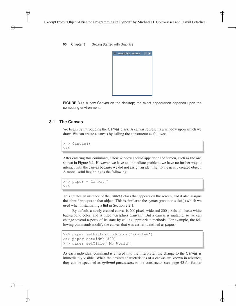
FIGURE 3.1: A new Canvas on the desktop; the exact appearance depends upon the

computing environment.

3.1 The Canvas

We begin by introducing the Canvas class. A canvas represents a window upon which we

draw. We can create a canvas by calling the constructor as follows:

>>> Canvas()

>>>

After entering this command, a new window should appear on the screen, such as the one

shown in Figure 3.1. However, we have an immediate problem; we have no further way to

interact with the canvas because we did not assign an identifier to the newly created object.

A more useful beginning is the following:

>>> paper = Canvas()

>>>

This creates an instance of the Canvas class that appears on the screen, and it also assigns

the identifier paper to that object. This is similar to the syntax groceries = list( ) which we

used when instantiating a list in Section 2.2.1.

By default, a newly created canvas is 200 pixels wide and 200 pixels tall, has a white

background color, and is titled “Graphics Canvas.” But a canvas is mutable, so we can

change several aspects of its state by calling appropriate methods. For example, the fol-

lowing commands modify the canvas that was earlier identified as paper:

>>> paper.setBackgroundColor('skyBlue')

>>> paper.setWidth(300)

>>> paper.setTitle('My World')

As each individual command is entered into the interpreter, the change to the Canvas is

immediately visible. When the desired characteristics of a canvas are known in advance,

they can be specified as optional parameters to the constructor (see page 43 for further


Section 3.1 The Canvas 91

Canvas

Canvas(w, h, bgColor, title, autoRefresh) add(drawable)

getWidth( ) remove(drawable)

setWidth(w) clear( )

getHeight( ) open( )

setHeight(h) close( )

getBackgroundColor( ) saveToFile(filename)

setBackgroundColor(color) setAutoRefresh(trueOrFalse)

getTitle( ) refresh( )

setTitle(title) wait( )

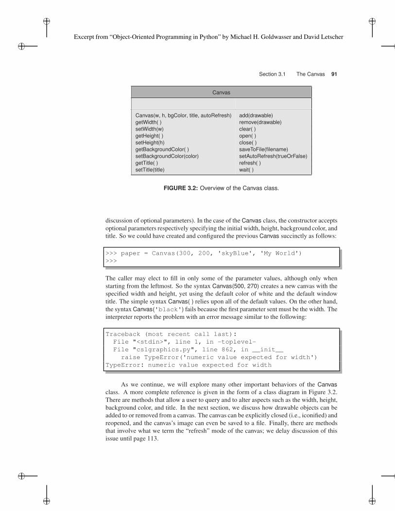
FIGURE 3.2: Overview of the Canvas class.

discussion of optional parameters). In the case of the Canvas class, the constructor accepts

optional parameters respectively specifying the initial width, height, background color, and

title. So we could have created and configured the previous Canvas succinctly as follows:

>>> paper = Canvas(300, 200, 'skyBlue', 'My World')

>>>

The caller may elect to fill in only some of the parameter values, although only when

starting from the leftmost. So the syntax Canvas(500, 270) creates a new canvas with the

specified width and height, yet using the default color of white and the default window

title. The simple syntax Canvas( ) relies upon all of the default values. On the other hand,

the syntax Canvas('black') fails because the first parameter sent must be the width. The

interpreter reports the problem with an error message similar to the following:

Traceback (most recent call last) :

File "<stdin>", line 1, in -toplevel-

File "cs1graphics.py", line 862, in __init__

raise TypeError('numeric value expected for width')

TypeError : numeric value expected for width

As we continue, we will explore many other important behaviors of the Canvas

class. A more complete reference is given in the form of a class diagram in Figure 3.2.

There are methods that allow a user to query and to alter aspects such as the width, height,

background color, and title. In the next section, we discuss how drawable objects can be

added to or removed from a canvas. The canvas can be explicitly closed (i.e., iconified) and

reopened, and the canvas’s image can even be saved to a file. Finally, there are methods

that involve what we term the “refresh” mode of the canvas; we delay discussion of this

issue until page 113.



y−axis

x−axis

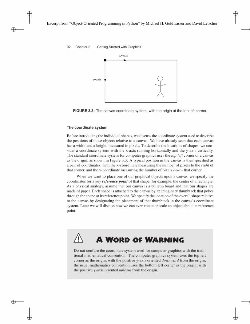
FIGURE 3.3: The canvas coordinate system, with the origin at the top left corner.

The coordinate system

Before introducing the individual shapes, we discuss the coordinate system used to describe

the positions of those objects relative to a canvas. We have already seen that each canvas

has a width and a height, measured in pixels. To describe the locations of shapes, we con-

sider a coordinate system with the x-axis running horizontally and the y-axis vertically.

The standard coordinate system for computer graphics uses the top left corner of a canvas

as the origin, as shown in Figure 3.3. A typical position in the canvas is then specified as

a pair of coordinates, with the x-coordinate measuring the number of pixels to the right of

that corner, and the y-coordinate measuring the number of pixels below that corner.

When we want to place one of our graphical objects upon a canvas, we specify the

coordinates for a key reference point of that shape, for example, the center of a rectangle.

As a physical analogy, assume that our canvas is a bulletin board and that our shapes are

made of paper. Each shape is attached to the canvas by an imaginary thumbtack that pokes

through the shape at its reference point. We specify the location of the overall shape relative

to the canvas by designating the placement of that thumbtack in the canvas’s coordinate

system. Later we will discuss how we can even rotate or scale an object about its reference

point.

Do not confuse the coordinate system used for computer graphics with the tradi-

tional mathematical convention. The computer graphics system uses the top left

corner as the origin, with the positive y-axis oriented downward from the origin;

the usual mathematics convention uses the bottom left corner as the origin, with

the positive y-axis oriented upward from the origin.


Section 3.2 Drawable Objects 93

3.2 Drawable Objects

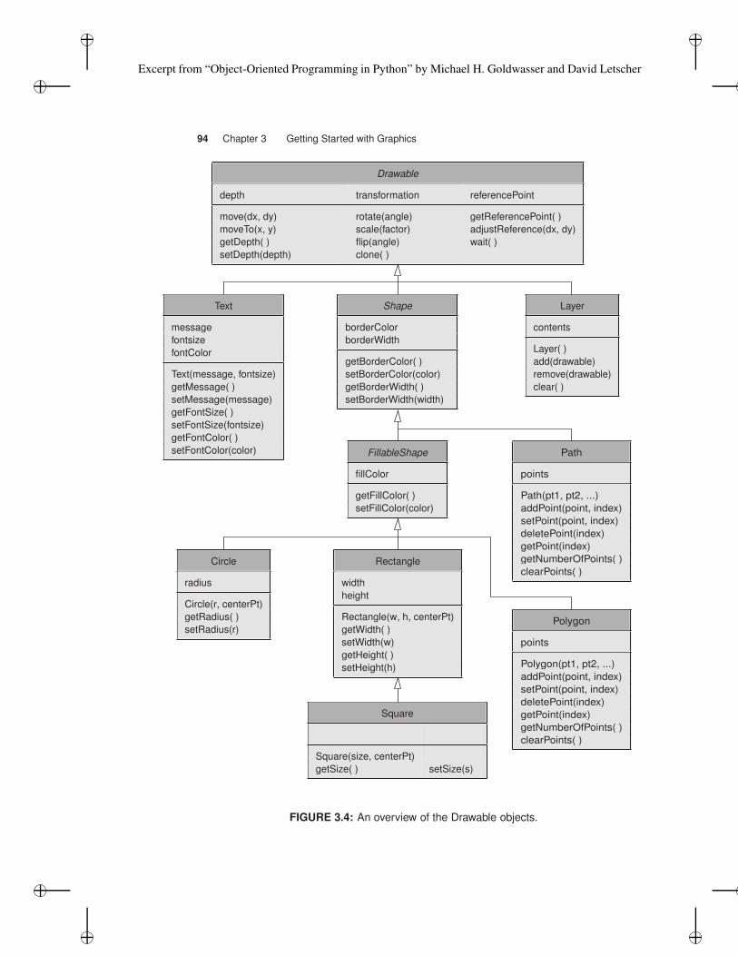
The cs1graphics module supports a variety of objects that can be drawn onto a canvas.

These objects are organized in a class hierarchy originally modeled in Section 1.4.4. A

more detailed summary of the various classes is given in Figure 3.4. This diagram is packed

with information and may seem overwhelming at first, but it provides a nice summary that

can be used as a reference. The use of inheritance emphasizes the similarities, making it

easier to learn how to use each class.

When examining this diagram, remember that classes in a hierarchy inherit methods

from their parent class. For example, each type of FillableShape supports a setFillColor

method. So not only does a Circle support the setRadius method, but also the setFillColor

method due to its parent class, and the setBorderWidth method due to its grandparent

Shape class. Many of the names should be self-explanatory and formal documentation

for each class can be viewed directly in the Python interpreter as you work. For example,

complete documentation for the Circle class can be viewed by typing help(Circle) at the

Python prompt.

Once you know how to create and manipulate circles, it will not take much effort

to learn to create and manipulate squares. Circles and squares are not identical; there are

a few ways in which they differ. But there are significantly more ways in which they are

similar. To demonstrate the basic use of the individual classes, we spend the rest of this

section composing a simple picture of a house with scenery. This example does not show

every single feature of the graphics library, but it should provide a good introduction.

Circle

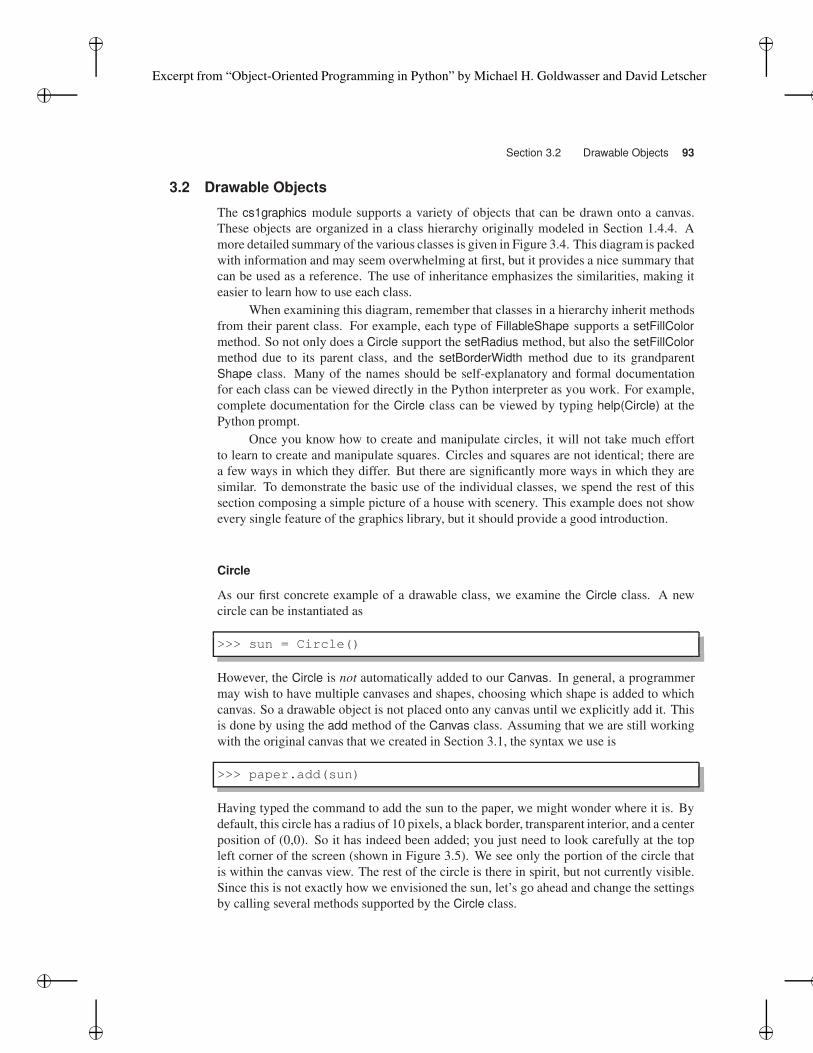
As our first concrete example of a drawable class, we examine the Circle class. A new

circle can be instantiated as

>>> sun = Circle()

However, the Circle is not automatically added to our Canvas. In general, a programmer

may wish to have multiple canvases and shapes, choosing which shape is added to which

canvas. So a drawable object is not placed onto any canvas until we explicitly add it. This

is done by using the add method of the Canvas class. Assuming that we are still working

with the original canvas that we created in Section 3.1, the syntax we use is

>>> paper.add(sun)

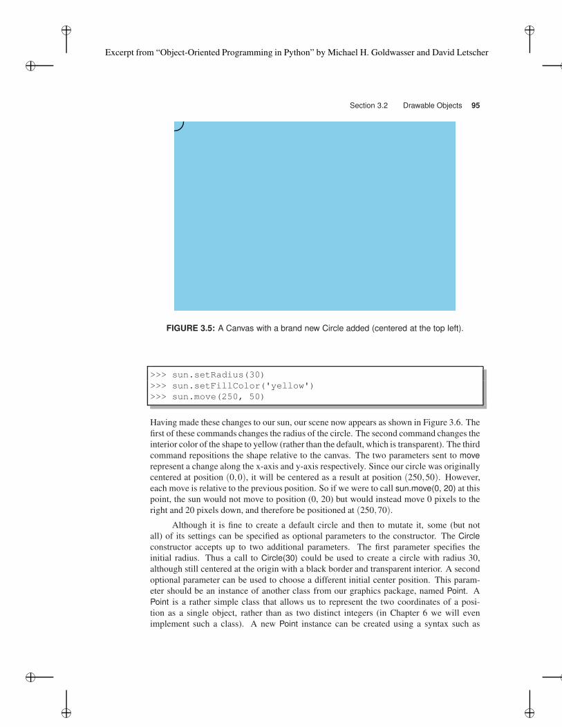
Having typed the command to add the sun to the paper, we might wonder where it is. By

default, this circle has a radius of 10 pixels, a black border, transparent interior, and a center

position of (0,0). So it has indeed been added; you just need to look carefully at the top

left corner of the screen (shown in Figure 3.5). We see only the portion of the circle that

is within the canvas view. The rest of the circle is there in spirit, but not currently visible.

Since this is not exactly how we envisioned the sun, let’s go ahead and change the settings

by calling several methods supported by the Circle class.



Rectangle

width

height

Rectangle(w, h, centerPt)

getWidth( )

setWidth(w)

getHeight( )

setHeight(h)

Shape

borderColor

borderWidth

getBorderColor( )

setBorderColor(color)

getBorderWidth( )

setBorderWidth(width)

Text

message

fontsize

fontColor

Text(message, fontsize)

getMessage( )

setMessage(message)

getFontSize( )

setFontSize(fontsize)

getFontColor( )

setFontColor(color)

Layer

contents

Layer( )

add(drawable)

remove(drawable)

clear( )

Path

points

Path(pt1, pt2, ...)

addPoint(point, index)

setPoint(point, index)

deletePoint(index)

getPoint(index)

getNumberOfPoints( )

clearPoints( )

Polygon

points

Polygon(pt1, pt2, ...)

addPoint(point, index)

setPoint(point, index)

deletePoint(index)

getPoint(index)

getNumberOfPoints( )

clearPoints( )

Square

Square(size, centerPt)

getSize( ) setSize(s)

FillableShape

fillColor

getFillColor( )

setFillColor(color)

Drawable

depth transformation referencePoint

move(dx, dy) rotate(angle) getReferencePoint( )

moveTo(x, y) scale(factor) adjustReference(dx, dy)

getDepth( ) flip(angle) wait( )

setDepth(depth) clone( )

Circle

radius

Circle(r, centerPt)

getRadius( )

setRadius(r)

FIGURE 3.4: An overview of the Drawable objects.



FIGURE 3.5: A Canvas with a brand new Circle added (centered at the top left).

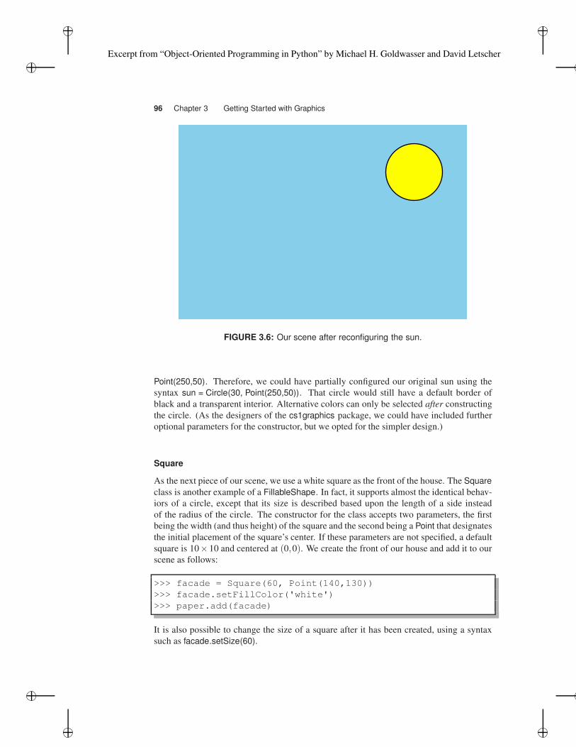
>>> sun.setRadius(30)

>>> sun.setFillColor('yellow')

>>> sun.move(250, 50)

Having made these changes to our sun, our scene now appears as shown in Figure 3.6. The

first of these commands changes the radius of the circle. The second command changes the

interior color of the shape to yellow (rather than the default, which is transparent). The third

command repositions the shape relative to the canvas. The two parameters sent to move

represent a change along the x-axis and y-axis respectively. Since our circle was originally

centered at position (0,0), it will be centered as a result at position (250,50). However,

each move is relative to the previous position. So if we were to call sun.move(0, 20) at this

point, the sun would not move to position (0, 20) but would instead move 0 pixels to the

right and 20 pixels down, and therefore be positioned at (250,70).

Although it is fine to create a default circle and then to mutate it, some (but not

all) of its settings can be specified as optional parameters to the constructor. The Circle

constructor accepts up to two additional parameters. The first parameter specifies the

initial radius. Thus a call to Circle(30) could be used to create a circle with radius 30,

although still centered at the origin with a black border and transparent interior. A second

optional parameter can be used to choose a different initial center position. This param-

eter should be an instance of another class from our graphics package, named Point. A

Point is a rather simple class that allows us to represent the two coordinates of a posi-

tion as a single object, rather than as two distinct integers (in Chapter 6 we will even

implement such a class). A new Point instance can be created using a syntax such as



FIGURE 3.6: Our scene after reconfiguring the sun.

Point(250,50). Therefore, we could have partially configured our original sun using the

syntax sun = Circle(30, Point(250,50)). That circle would still have a default border of

black and a transparent interior. Alternative colors can only be selected after constructing

the circle. (As the designers of the cs1graphics package, we could have included further

optional parameters for the constructor, but we opted for the simpler design.)

Square

As the next piece of our scene, we use a white square as the front of the house. The Square

class is another example of a FillableShape. In fact, it supports almost the identical behav-

iors of a circle, except that its size is described based upon the length of a side instead

of the radius of the circle. The constructor for the class accepts two parameters, the first

being the width (and thus height) of the square and the second being a Point that designates

the initial placement of the square’s center. If these parameters are not specified, a default

square is 10×10 and centered at (0,0). We create the front of our house and add it to our

scene as follows:

>>> facade = Square(60, Point(140,130))

>>> facade.setFillColor('white')

>>> paper.add(facade)

It is also possible to change the size of a square after it has been created, using a syntax

such as facade.setSize(60).



Rectangle

Another available shape is a Rectangle, which is similar to a Square except that we can

set its width and height independently. By default, a rectangle has a width of 20 pixels,

a height of 10 pixels, and is centered at the origin. However, the initial geometry can be

specified using three optional parameters to the constructor, respectively specifying the

width, the height, and the center point. Adding to our ongoing picture, we place a chimney

on top of our house with the following commands:

>>> chimney = Rectangle(15, 28, Point(155,85))

>>> chimney.setFillColor('red')

>>> paper.add(chimney)

We carefully design the geometry so that the chimney appears to rest on top of the right

side of the house. Recall that the facade is a 60-pixel square centered with a y-coordinate

of 130. So the top edge of that facade has a y-coordinate of 100. To rest above, our

chimney is centered vertically at 85 but with a height of 28. So it extends along the y-axis

from 71 to 99. Alternatively, we could have waited until after the rectangle had been

constructed to adjust those settings, using the setWidth and setHeight methods.

We take this opportunity to distinguish between the interior of a shape and its border.

The chimney as described above has a red interior but a thin black outline. For all of

the shapes we have seen thus far, we can separately control the color of the interior, via

setFillColor, and the color of the border, via setBorderColor. If we want to get rid of

the border for our chimney, we can accomplish this in one of three ways. The first is

chimney.setBorderColor('red'). This does not really get rid of the border but colors

it the same as the interior. It is also possible to set the border color to a special color

'Transparent', in which case it is not even drawn. Finally, we can adjust the width

of the border itself. A call to chimney.setBorderWidth(0) should make the border unseen,

even if it were still designated as black.

Polygon

The Polygon class provides a much more general shape, allowing for filled polygons with

arbitrarily many sides. The geometry of a polygon is specified by identifying the position

of each corner, as ordered along the boundary. As was the case with other shapes, the

initial geometry of a polygon can be specified using optional parameters to the constructor.

Because polygons may have many points, the constructor accepts an arbitrary number of

points as optional parameters. For example, we might add an evergreen tree to our scene

by creating a green triangle as follows:

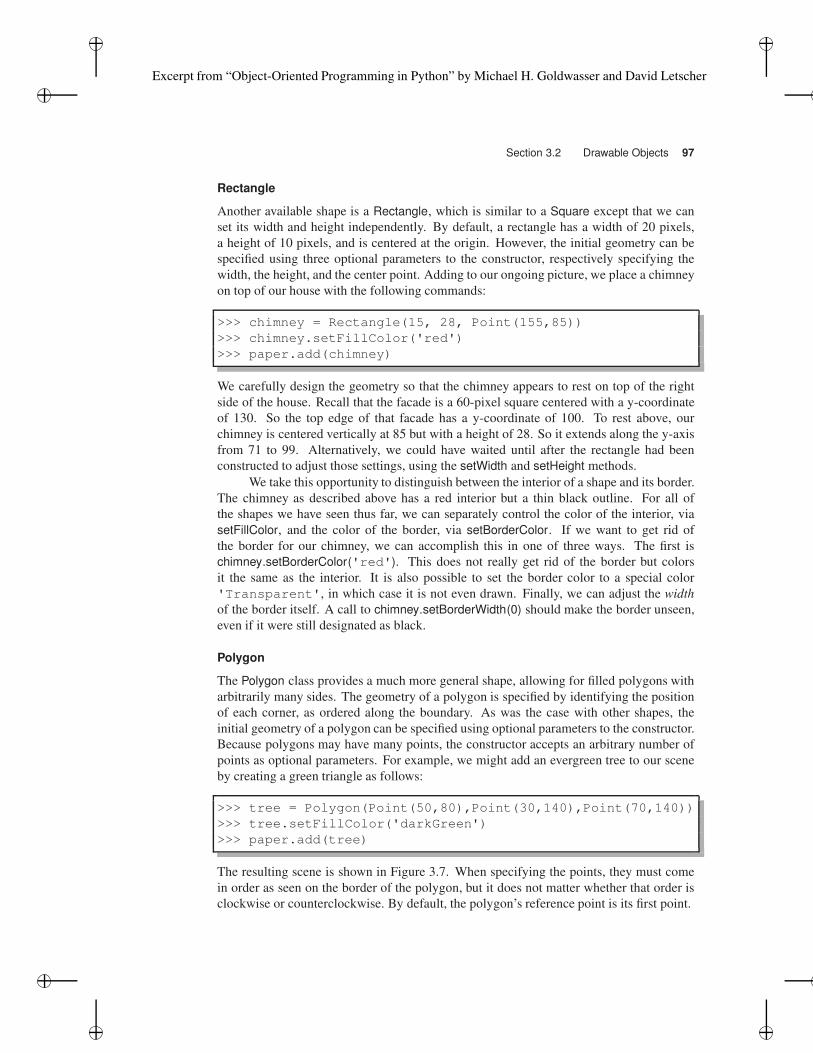
>>> tree = Polygon(Point(50,80),Point(30,140),Point(70,140))

>>> tree.setFillColor('darkGreen')

>>> paper.add(tree)

The resulting scene is shown in Figure 3.7. When specifying the points, they must come

in order as seen on the border of the polygon, but it does not matter whether that order is

clockwise or counterclockwise. By default, the polygon’s reference point is its first point.



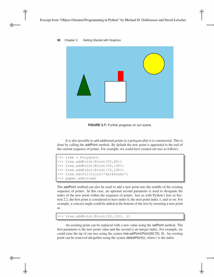
FIGURE 3.7: Further progress on our scene.

It is also possible to add additional points to a polygon after it is constructed. This is

done by calling the addPoint method. By default the new point is appended to the end of

the current sequence of points. For example, we could have created our tree as follows:

>>> tree = Polygon()

>>> tree.addPoint(Point(50,80))



>>> tree.setFillColor('darkGreen')

>>> paper.add(tree)

The addPoint method can also be used to add a new point into the middle of the existing

sequence of points. In this case, an optional second parameter is used to designate the

index of the new point within the sequence of points. Just as with Python’s lists in Sec-

tion 2.2, the first point is considered to have index 0, the next point index 1, and so on. For

example, a concave angle could be added at the bottom of the tree by inserting a new point

as

>>> tree.addPoint(Point(50,120), 2)

An existing point can be replaced with a new value using the setPoint method. The

first parameter is the new point value and the second is an integer index. For example, we

could raise the tip of our tree using the syntax tree.setPoint(Point(50,70), 0). An existing

point can be removed altogether using the syntax deletePoint(i), where i is the index.



Path

A Path is a shape that connects a series of points; in this respect, it is very similar to a

Polygon. However, there are two key differences: the ends of a path are not explicitly con-

nected to each other, and a path does not have an interior. A Path qualifies in our hierarchy

as a Shape but not as a FillableShape. We can change the color by calling setBorderColor,

and the thickness by calling setBorderWidth. Its behaviors are otherwise similar to those

described for the Polygon (e.g., addPoint, setPoint, deletePoint). As a simple example of

a path, we add a bit of smoke coming out of the top of our chimney.

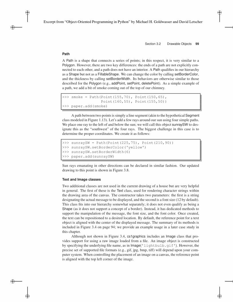
>>> smoke = Path(Point(155,70), Point(150,65),

Point(160,55), Point(155,50))

>>> paper.add(smoke)

A path between two points is simply a line segment (akin to the hypothetical Segment

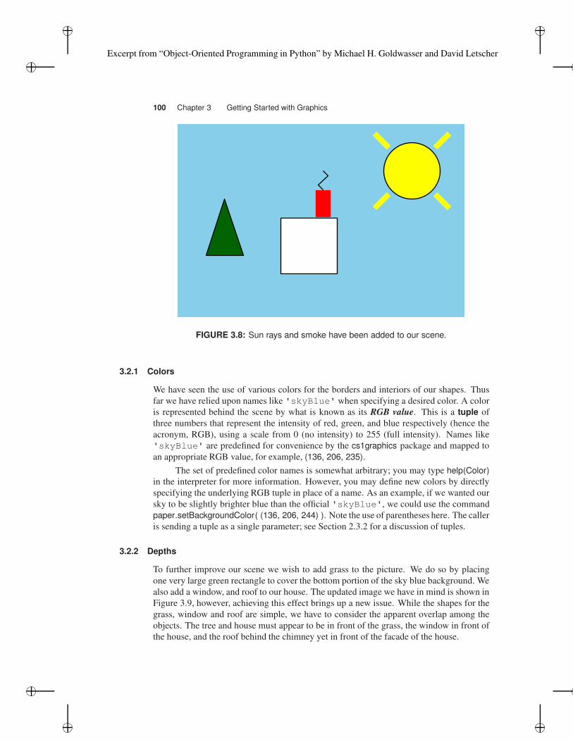
class modeled in Figure 1.13). Let’s add a few rays around our sun using four simple paths.

We place one ray to the left of and below the sun; we will call this object sunraySW to des-

ignate this as the “southwest” of the four rays. The biggest challenge in this case is to

determine the proper coordinates. We create it as follows:

>>> sunraySW = Path(Point(225,75), Point(210,90))

>>> sunraySW.setBorderColor('yellow')

>>> sunraySW.setBorderWidth(6)

>>> paper.add(sunraySW)

Sun rays emanating in other directions can be declared in similar fashion. Our updated

drawing to this point is shown in Figure 3.8.

Text and Image classes

Two additional classes are not used in the current drawing of a house but are very helpful

in general. The first of these is the Text class, used for rendering character strings within

the drawing area of the canvas. The constructor takes two parameters: the first is a string

designating the actual message to be displayed, and the second is a font size (12 by default).

This class fits into our hierarchy somewhat separately; it does not even qualify as being a

Shape (as it does not support a concept of a border). Instead, it has dedicated methods to

support the manipulation of the message, the font size, and the font color. Once created,

the text can be repositioned to a desired location. By default, the reference point for a text

object is aligned with the center of the displayed message. The summary of its methods is

included in Figure 3.4 on page 94; we provide an example usage in a later case study in

this chapter.

Although not shown in Figure 3.4, cs1graphics includes an Image class that pro-

vides support for using a raw image loaded from a file. An image object is constructed

by specifying the underlying file name, as in Image('lightbulb.gif'). However, the

precise set of supported file formats (e.g., gif, jpg, bmp, tiff) will depend upon your com-

puter system. When controlling the placement of an image on a canvas, the reference point

is aligned with the top left corner of the image.



FIGURE 3.8: Sun rays and smoke have been added to our scene.

3.2.1 Colors

We have seen the use of various colors for the borders and interiors of our shapes. Thus

far we have relied upon names like 'skyBlue' when specifying a desired color. A color

is represented behind the scene by what is known as its RGB value. This is a tuple of

three numbers that represent the intensity of red, green, and blue respectively (hence the

acronym, RGB), using a scale from 0 (no intensity) to 255 (full intensity). Names like

'skyBlue' are predefined for convenience by the cs1graphics package and mapped to

an appropriate RGB value, for example, (136, 206, 235).

The set of predefined color names is somewhat arbitrary; you may type help(Color)

in the interpreter for more information. However, you may define new colors by directly

specifying the underlying RGB tuple in place of a name. As an example, if we wanted our

sky to be slightly brighter blue than the official 'skyBlue', we could use the command

paper.setBackgroundColor( (136, 206, 244) ). Note the use of parentheses here. The caller

is sending a tuple as a single parameter; see Section 2.3.2 for a discussion of tuples.

3.2.2 Depths

To further improve our scene we wish to add grass to the picture. We do so by placing

one very large green rectangle to cover the bottom portion of the sky blue background. We

also add a window, and roof to our house. The updated image we have in mind is shown in

Figure 3.9, however, achieving this effect brings up a new issue. While the shapes for the

grass, window and roof are simple, we have to consider the apparent overlap among the

objects. The tree and house must appear to be in front of the grass, the window in front of

the house, and the roof behind the chimney yet in front of the facade of the house.



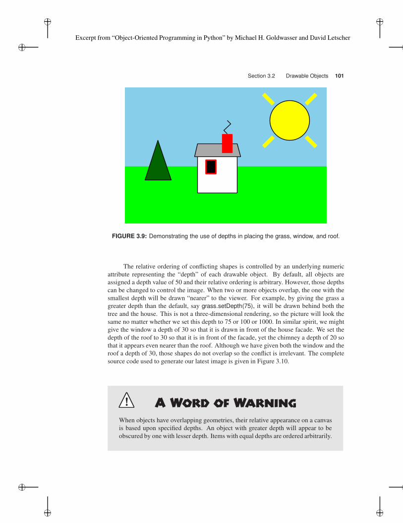
FIGURE 3.9: Demonstrating the use of depths in placing the grass, window, and roof.

The relative ordering of conflicting shapes is controlled by an underlying numeric

attribute representing the “depth” of each drawable object. By default, all objects are

assigned a depth value of 50 and their relative ordering is arbitrary. However, those depths

can be changed to control the image. When two or more objects overlap, the one with the

smallest depth will be drawn “nearer” to the viewer. For example, by giving the grass a

greater depth than the default, say grass.setDepth(75), it will be drawn behind both the

tree and the house. This is not a three-dimensional rendering, so the picture will look the

same no matter whether we set this depth to 75 or 100 or 1000. In similar spirit, we might

give the window a depth of 30 so that it is drawn in front of the house facade. We set the

depth of the roof to 30 so that it is in front of the facade, yet the chimney a depth of 20 so

that it appears even nearer than the roof. Although we have given both the window and the

roof a depth of 30, those shapes do not overlap so the conflict is irrelevant. The complete

source code used to generate our latest image is given in Figure 3.10.

When objects have overlapping geometries, their relative appearance on a canvas

is based upon specified depths. An object with greater depth will appear to be

obscured by one with lesser depth. Items with equal depths are ordered arbitrarily.



1 from cs1graphics import *2 paper = Canvas(300, 200, 'skyBlue', 'My World')

3

4 sun = Circle(30, Point(250,50))

5 sun.setFillColor('yellow')

6 paper.add(sun)

7

8 facade = Square(60, Point(140,130))

9 facade.setFillColor('white')

10 paper.add(facade)

11

12 chimney = Rectangle(15, 28, Point(155,85))

13 chimney.setFillColor('red')

14 chimney.setBorderColor('red')

15 paper.add(chimney)

16

17 tree = Polygon(Point(50,80), Point(30,140), Point(70,140))

18 tree.setFillColor('darkGreen')

19 paper.add(tree)

20

21 smoke = Path(Point(155,70), Point(150,65), Point(160,55), Point(155,50))

22 paper.add(smoke)

23

24 sunraySW = Path(Point(225,75), Point(210,90))

25 sunraySW.setBorderColor('yellow')

26 sunraySW.setBorderWidth(6)

27 paper.add(sunraySW)

28 sunraySE = Path(Point(275,75), Point(290,90))

29 sunraySE.setBorderColor('yellow')

30 sunraySE.setBorderWidth(6)

31 paper.add(sunraySE)

32 sunrayNE = Path(Point(275,25), Point(290,10))

33 sunrayNE.setBorderColor('yellow')

34 sunrayNE.setBorderWidth(6)

35 paper.add(sunrayNE)

36 sunrayNW = Path(Point(225,25), Point(210,10))

37 sunrayNW.setBorderColor('yellow')

38 sunrayNW.setBorderWidth(6)

39 paper.add(sunrayNW)

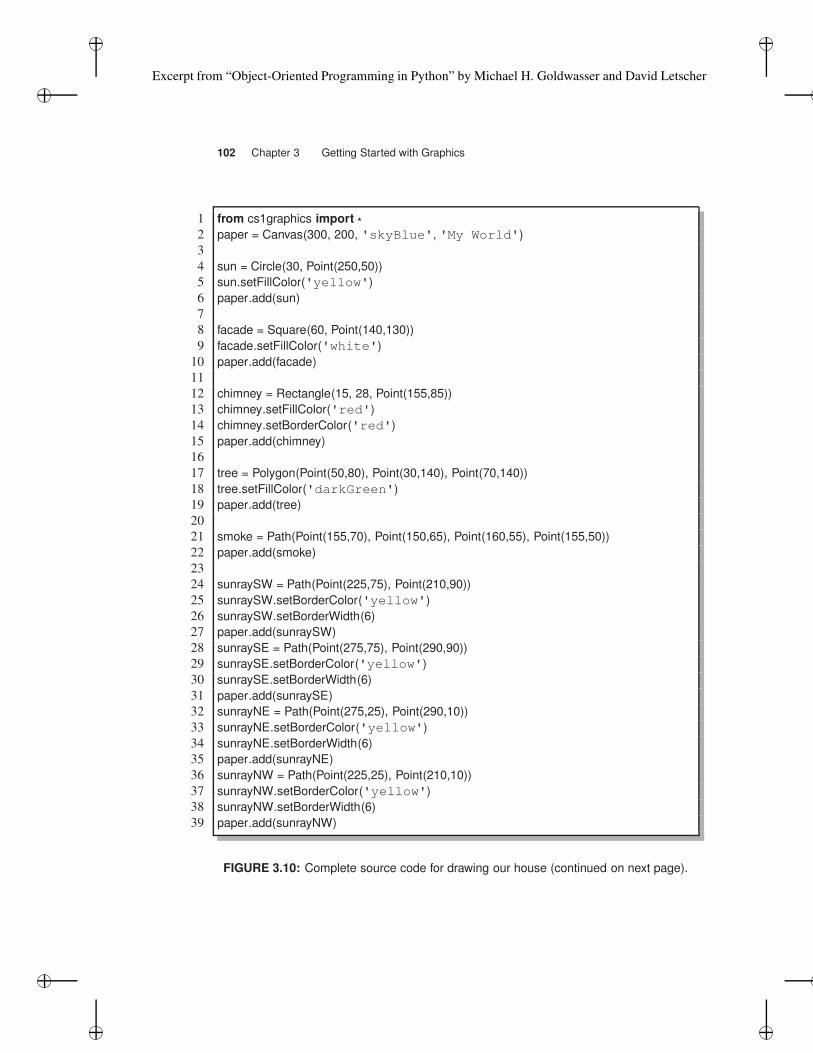
FIGURE 3.10: Complete source code for drawing our house (continued on next page).


Section 3.3 Rotating, Scaling, and Flipping 103

40 grass = Rectangle(300, 80, Point(150,160))

41 grass.setFillColor('green')

42 grass.setBorderColor('green')

43 grass.setDepth(75) # must be behind house and tree

44 paper.add(grass)

45

46 window = Rectangle(15, 20, Point(130,120))

47 paper.add(window)

48 window.setFillColor('black')

49 window.setBorderColor('red')

50 window.setBorderWidth(2)

51 window.setDepth(30)

52

53 roof = Polygon(Point(105, 105), Point(175, 105), Point(170,85), Point(110,85))

54 roof.setFillColor('darkgray')

55 roof.setDepth(30) # in front of facade

56 chimney.setDepth(20) # in front of roof

57 paper.add(roof)

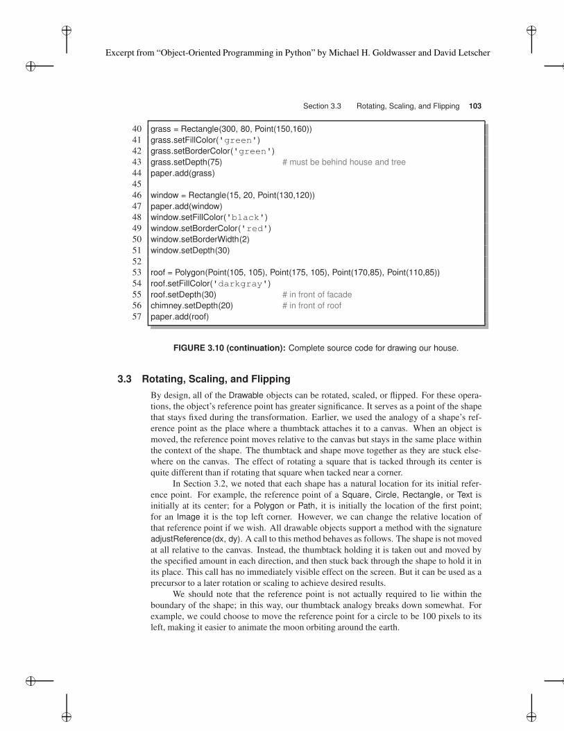
FIGURE 3.10 (continuation): Complete source code for drawing our house.

3.3 Rotating, Scaling, and Flipping

By design, all of the Drawable objects can be rotated, scaled, or flipped. For these opera-

tions, the object’s reference point has greater significance. It serves as a point of the shape

that stays fixed during the transformation. Earlier, we used the analogy of a shape’s ref-

erence point as the place where a thumbtack attaches it to a canvas. When an object is

moved, the reference point moves relative to the canvas but stays in the same place within

the context of the shape. The thumbtack and shape move together as they are stuck else-

where on the canvas. The effect of rotating a square that is tacked through its center is

quite different than if rotating that square when tacked near a corner.

In Section 3.2, we noted that each shape has a natural location for its initial refer-

ence point. For example, the reference point of a Square, Circle, Rectangle, or Text is

initially at its center; for a Polygon or Path, it is initially the location of the first point;

for an Image it is the top left corner. However, we can change the relative location of

that reference point if we wish. All drawable objects support a method with the signature

adjustReference(dx, dy). A call to this method behaves as follows. The shape is not moved

at all relative to the canvas. Instead, the thumbtack holding it is taken out and moved by

the specified amount in each direction, and then stuck back through the shape to hold it in

its place. This call has no immediately visible effect on the screen. But it can be used as a

precursor to a later rotation or scaling to achieve desired results.

We should note that the reference point is not actually required to lie within the

boundary of the shape; in this way, our thumbtack analogy breaks down somewhat. For

example, we could choose to move the reference point for a circle to be 100 pixels to its

left, making it easier to animate the moon orbiting around the earth.



Rotating

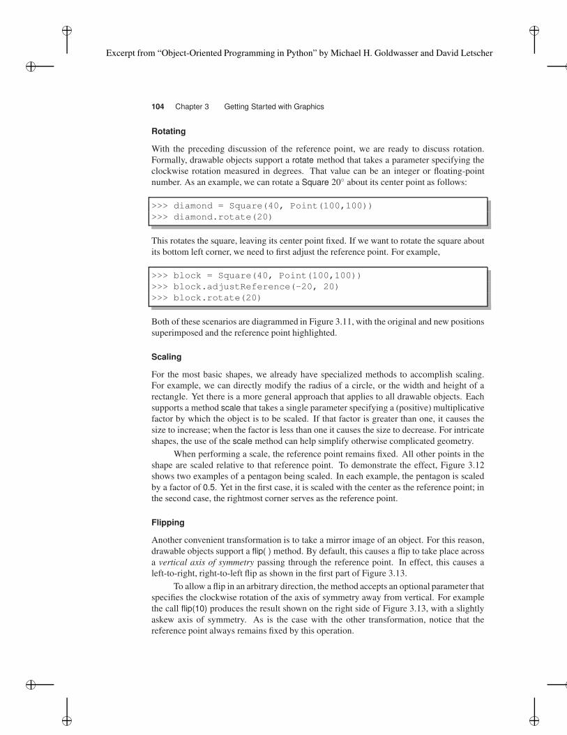
With the preceding discussion of the reference point, we are ready to discuss rotation.

Formally, drawable objects support a rotate method that takes a parameter specifying the

clockwise rotation measured in degrees. That value can be an integer or floating-point

number. As an example, we can rotate a Square 20◦ about its center point as follows:

>>> diamond = Square(40, Point(100,100))

>>> diamond.rotate(20)

This rotates the square, leaving its center point fixed. If we want to rotate the square about

its bottom left corner, we need to first adjust the reference point. For example,

>>> block = Square(40, Point(100,100))

>>> block.adjustReference(-20, 20)

>>> block.rotate(20)

Both of these scenarios are diagrammed in Figure 3.11, with the original and new positions

superimposed and the reference point highlighted.

Scaling

For the most basic shapes, we already have specialized methods to accomplish scaling.

For example, we can directly modify the radius of a circle, or the width and height of a

rectangle. Yet there is a more general approach that applies to all drawable objects. Each

supports a method scale that takes a single parameter specifying a (positive) multiplicative

factor by which the object is to be scaled. If that factor is greater than one, it causes the

size to increase; when the factor is less than one it causes the size to decrease. For intricate

shapes, the use of the scale method can help simplify otherwise complicated geometry.

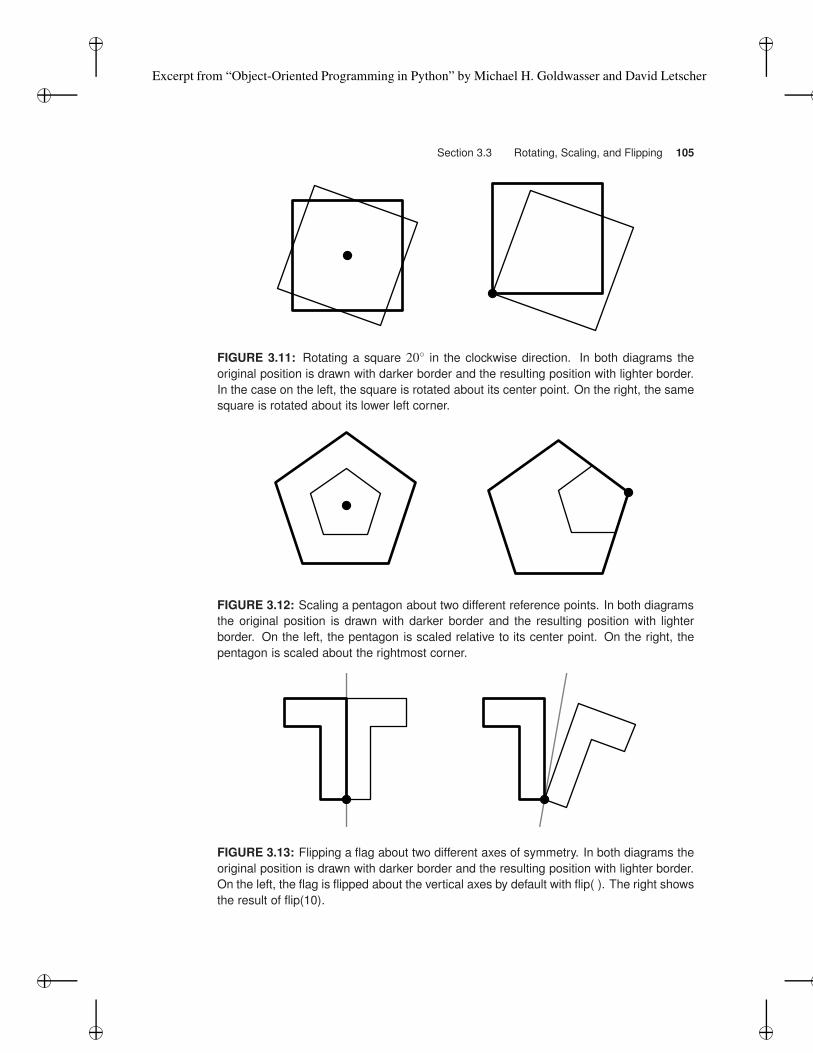
When performing a scale, the reference point remains fixed. All other points in the

shape are scaled relative to that reference point. To demonstrate the effect, Figure 3.12

shows two examples of a pentagon being scaled. In each example, the pentagon is scaled

by a factor of 0.5. Yet in the first case, it is scaled with the center as the reference point; in

the second case, the rightmost corner serves as the reference point.

Flipping

Another convenient transformation is to take a mirror image of an object. For this reason,

drawable objects support a flip( ) method. By default, this causes a flip to take place across

a vertical axis of symmetry passing through the reference point. In effect, this causes a

left-to-right, right-to-left flip as shown in the first part of Figure 3.13.

To allow a flip in an arbitrary direction, the method accepts an optional parameter that

specifies the clockwise rotation of the axis of symmetry away from vertical. For example

the call flip(10) produces the result shown on the right side of Figure 3.13, with a slightly

askew axis of symmetry. As is the case with the other transformation, notice that the

reference point always remains fixed by this operation.


Section 3.3 Rotating, Scaling, and Flipping 105

FIGURE 3.11: Rotating a square 20◦ in the clockwise direction. In both diagrams the

original position is drawn with darker border and the resulting position with lighter border.

In the case on the left, the square is rotated about its center point. On the right, the same

square is rotated about its lower left corner.

FIGURE 3.12: Scaling a pentagon about two different reference points. In both diagrams

the original position is drawn with darker border and the resulting position with lighter

border. On the left, the pentagon is scaled relative to its center point. On the right, the

pentagon is scaled about the rightmost corner.

FIGURE 3.13: Flipping a flag about two different axes of symmetry. In both diagrams the

original position is drawn with darker border and the resulting position with lighter border.

On the left, the flag is flipped about the vertical axes by default with flip( ). The right shows

the result of flip(10).



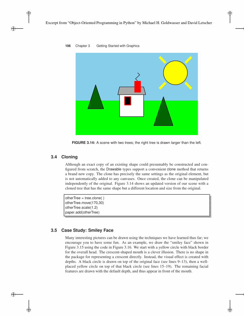
FIGURE 3.14: A scene with two trees; the right tree is drawn larger than the left.

3.4 Cloning

Although an exact copy of an existing shape could presumably be constructed and con-

figured from scratch, the Drawable types support a convenient clone method that returns

a brand new copy. The clone has precisely the same settings as the original element, but

is not automatically added to any canvases. Once created, the clone can be manipulated

independently of the original. Figure 3.14 shows an updated version of our scene with a

cloned tree that has the same shape but a different location and size from the original.

otherTree = tree.clone( )

otherTree.move(170,30)

otherTree.scale(1.2)

paper.add(otherTree)

3.5 Case Study: Smiley Face

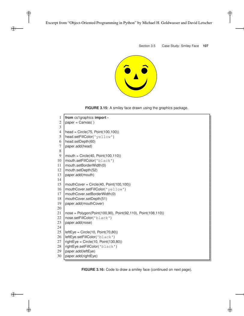
Many interesting pictures can be drawn using the techniques we have learned thus far; we

encourage you to have some fun. As an example, we draw the “smiley face” shown in

Figure 3.15 using the code in Figure 3.16. We start with a yellow circle with black border

for the overall head. The crescent-shaped mouth is a clever illusion. There is no shape in

the package for representing a crescent directly. Instead, the visual effect is created with

depths. A black circle is drawn on top of the original face (see lines 9–13), then a well-

placed yellow circle on top of that black circle (see lines 15–19). The remaining facial

features are drawn with the default depth, and thus appear in front of the mouth.


Section 3.5 Case Study: Smiley Face 107

FIGURE 3.15: A smiley face drawn using the graphics package.

1 from cs1graphics import *2 paper = Canvas( )

3

4 head = Circle(75, Point(100,100))

5 head.setFillColor('yellow')

6 head.setDepth(60)

7 paper.add(head)

8

9 mouth = Circle(40, Point(100,110))

10 mouth.setFillColor('black')

11 mouth.setBorderWidth(0)

12 mouth.setDepth(52)

13 paper.add(mouth)

14

15 mouthCover = Circle(40, Point(100,100))

16 mouthCover.setFillColor('yellow')

17 mouthCover.setBorderWidth(0)

18 mouthCover.setDepth(51)

19 paper.add(mouthCover)

20

21 nose = Polygon(Point(100,90), Point(92,110), Point(108,110))

22 nose.setFillColor('black')

23 paper.add(nose)

24

25 leftEye = Circle(10, Point(70,80))

26 leftEye.setFillColor('black')

27 rightEye = Circle(10, Point(130,80))

28 rightEye.setFillColor('black')

29 paper.add(leftEye)

30 paper.add(rightEye)

FIGURE 3.16: Code to draw a smiley face (continued on next page).



31 leftEyebrow = Path(Point(60,65), Point(70,60), Point(80,65))

32 leftEyebrow.setBorderWidth(3)

33 leftEyebrow.adjustReference(10,15) # set to center of left eyeball

34 leftEyebrow.rotate(−15)

35 paper.add(leftEyebrow)

36

37 rightEyebrow = leftEyebrow.clone( )

38 rightEyebrow.flip( ) # still relative to eyeball center

39 rightEyebrow.move(60,0) # distance between eyeball centers

40 paper.add(rightEyebrow)

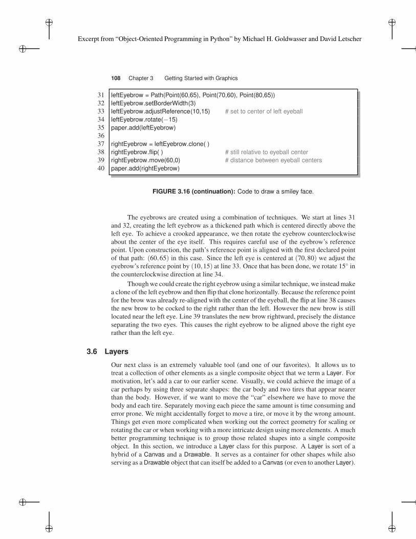
FIGURE 3.16 (continuation): Code to draw a smiley face.

The eyebrows are created using a combination of techniques. We start at lines 31

and 32, creating the left eyebrow as a thickened path which is centered directly above the

left eye. To achieve a crooked appearance, we then rotate the eyebrow counterclockwise

about the center of the eye itself. This requires careful use of the eyebrow’s reference

point. Upon construction, the path’s reference point is aligned with the first declared point

of that path: (60,65) in this case. Since the left eye is centered at (70,80) we adjust the

eyebrow’s reference point by (10,15) at line 33. Once that has been done, we rotate 15◦ in

the counterclockwise direction at line 34.

Though we could create the right eyebrow using a similar technique, we instead make

a clone of the left eyebrow and then flip that clone horizontally. Because the reference point

for the brow was already re-aligned with the center of the eyeball, the flip at line 38 causes

the new brow to be cocked to the right rather than the left. However the new brow is still

located near the left eye. Line 39 translates the new brow rightward, precisely the distance

separating the two eyes. This causes the right eyebrow to be aligned above the right eye

rather than the left eye.

3.6 Layers

Our next class is an extremely valuable tool (and one of our favorites). It allows us to

treat a collection of other elements as a single composite object that we term a Layer. For

motivation, let’s add a car to our earlier scene. Visually, we could achieve the image of a

car perhaps by using three separate shapes: the car body and two tires that appear nearer

than the body. However, if we want to move the “car” elsewhere we have to move the

body and each tire. Separately moving each piece the same amount is time consuming and

error prone. We might accidentally forget to move a tire, or move it by the wrong amount.

Things get even more complicated when working out the correct geometry for scaling or

rotating the car or when working with a more intricate design using more elements. A much

better programming technique is to group those related shapes into a single composite

object. In this section, we introduce a Layer class for this purpose. A Layer is sort of a

hybrid of a Canvas and a Drawable. It serves as a container for other shapes while also

serving as a Drawable object that can itself be added to a Canvas (or even to another Layer).


Section 3.6 Layers 109

Earlier, we explained our drawing package through the analogy of physical shapes

being attached to a canvas. We wish to extend this analogy to layers. We consider a layer

to be a thin clear film. We can attach many shapes directly to this film rather than to the

canvas. Of course the film itself can be positioned over the canvas and combined with other

shapes to make a complete image. In fact, this is precisely the technology that advanced

the creation of animated movies in the early 1900s. Rather than drawing the artwork on

a single piece of paper, different layers of the background and characters were separated

on clear sheets of celluloid. These were commonly called animation cels. The advantages

were great. The individual cels could still be layered, with appropriate depths, to produce

the desired result. Yet each cel could be moved and rotated independently of the others to

adjust the overall image. For example, a character could be on a cel of its own and then

moved across a background in successive frames.

We demonstrate the use of the Layer class by adding a car to our earlier house scene.

Before concerning ourselves with the overall scene, we compose the layer itself. A layer is

somewhat similar to a canvas in that it has its own relative coordinate system. Shapes can

be added to the layer, in which case the shape’s reference point determines the placement of

that shape relative to the layer’s coordinate system (i.e., the shape is tacked to a position on

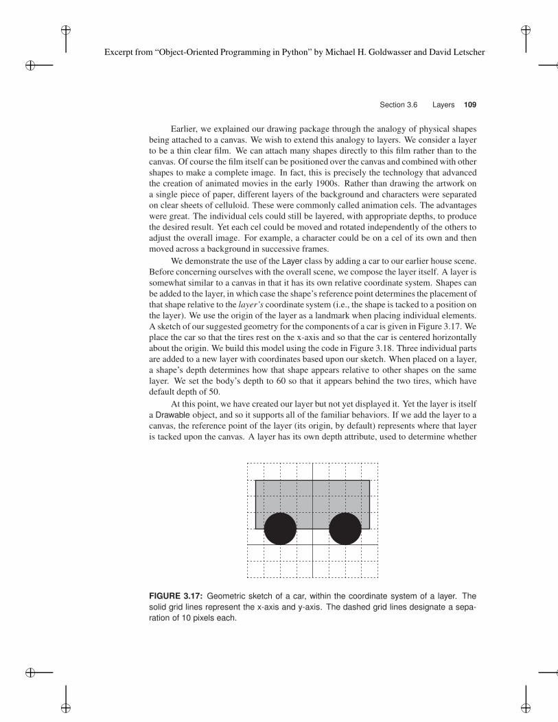
the layer). We use the origin of the layer as a landmark when placing individual elements.

A sketch of our suggested geometry for the components of a car is given in Figure 3.17. We

place the car so that the tires rest on the x-axis and so that the car is centered horizontally

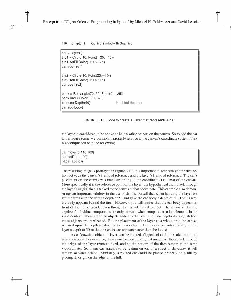
about the origin. We build this model using the code in Figure 3.18. Three individual parts

are added to a new layer with coordinates based upon our sketch. When placed on a layer,

a shape’s depth determines how that shape appears relative to other shapes on the same

layer. We set the body’s depth to 60 so that it appears behind the two tires, which have

default depth of 50.

At this point, we have created our layer but not yet displayed it. Yet the layer is itself

a Drawable object, and so it supports all of the familiar behaviors. If we add the layer to a

canvas, the reference point of the layer (its origin, by default) represents where that layer

is tacked upon the canvas. A layer has its own depth attribute, used to determine whether

FIGURE 3.17: Geometric sketch of a car, within the coordinate system of a layer. The

solid grid lines represent the x-axis and y-axis. The dashed grid lines designate a sepa-

ration of 10 pixels each.



car = Layer( )

tire1 = Circle(10, Point(−20,−10))

tire1.setFillColor('black')

car.add(tire1)

tire2 = Circle(10, Point(20,−10))

tire2.setFillColor('black')

car.add(tire2)

body = Rectangle(70, 30, Point(0, −25))

body.setFillColor('blue')

body.setDepth(60) # behind the tires

car.add(body)

FIGURE 3.18: Code to create a Layer that represents a car.

the layer is considered to be above or below other objects on the canvas. So to add the car

to our house scene, we position in properly relative to the canvas’s coordinate system. This

is accomplished with the following:

car.moveTo(110,180)

car.setDepth(20)

paper.add(car)

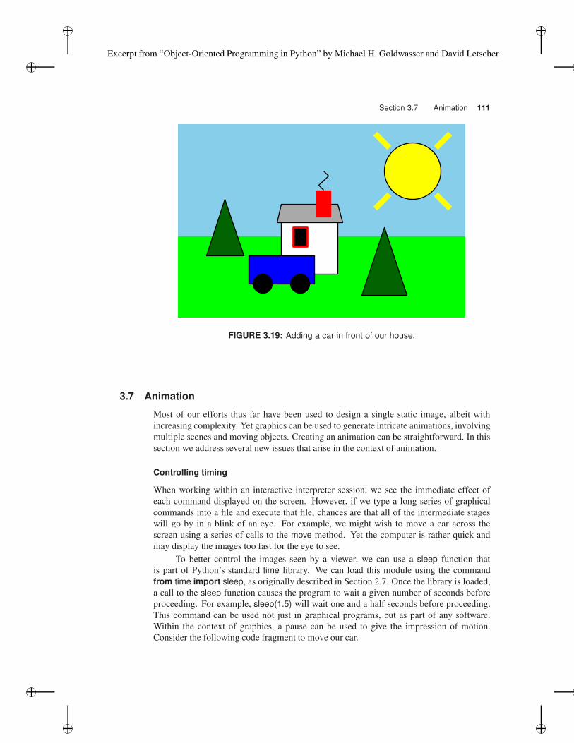
The resulting image is portrayed in Figure 3.19. It is important to keep straight the distinc-

tion between the canvas’s frame of reference and the layer’s frame of reference. The car’s

placement on the canvas was made according to the coordinate (110, 180) of the canvas.

More specifically it is the reference point of the layer (the hypothetical thumbtack through

the layer’s origin) that is tacked to the canvas at that coordinate. This example also demon-

strates an important subtlety in the use of depths. Recall that when building the layer we

left the tires with the default depth of 50 and gave the car body a depth of 60. That is why

the body appears behind the tires. However, you will notice that the car body appears in

front of the house facade, even though that facade has depth 50. The reason is that the

depths of individual components are only relevant when compared to other elements in the

same context. There are three objects added to the layer and their depths distinguish how

those objects are interleaved. But the placement of the layer as a whole onto the canvas

is based upon the depth attribute of the layer object. In this case we intentionally set the

layer’s depth to 30 so that the entire car appears nearer than the house.

As a Drawable object, a layer can be rotated, flipped, cloned, or scaled about its

reference point. For example, if we were to scale our car, that imaginary thumbtack through

the origin of the layer remains fixed, and so the bottom of the tires remain at the same

y-coordinate. So if our car appears to be resting on top of a street or driveway, it will

remain so when scaled. Similarly, a rotated car could be placed properly on a hill by

placing its origin on the edge of the hill.


Section 3.7 Animation 111

FIGURE 3.19: Adding a car in front of our house.

3.7 Animation

Most of our efforts thus far have been used to design a single static image, albeit with

increasing complexity. Yet graphics can be used to generate intricate animations, involving

multiple scenes and moving objects. Creating an animation can be straightforward. In this

section we address several new issues that arise in the context of animation.

Controlling timing

When working within an interactive interpreter session, we see the immediate effect of

each command displayed on the screen. However, if we type a long series of graphical

commands into a file and execute that file, chances are that all of the intermediate stages

will go by in a blink of an eye. For example, we might wish to move a car across the

screen using a series of calls to the move method. Yet the computer is rather quick and

may display the images too fast for the eye to see.

To better control the images seen by a viewer, we can use a sleep function that

is part of Python’s standard time library. We can load this module using the command

from time import sleep, as originally described in Section 2.7. Once the library is loaded,

a call to the sleep function causes the program to wait a given number of seconds before

proceeding. For example, sleep(1.5) will wait one and a half seconds before proceeding.

This command can be used not just in graphical programs, but as part of any software.

Within the context of graphics, a pause can be used to give the impression of motion.

Consider the following code fragment to move our car.



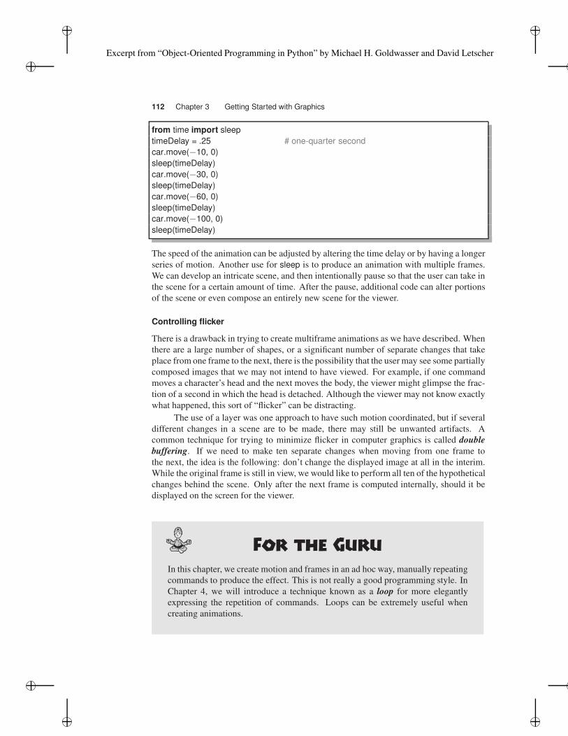
from time import sleep

timeDelay = .25 # one-quarter second

car.move(−10, 0)

sleep(timeDelay)

car.move(−30, 0)

sleep(timeDelay)

car.move(−60, 0)

sleep(timeDelay)

car.move(−100, 0)

sleep(timeDelay)

The speed of the animation can be adjusted by altering the time delay or by having a longer

series of motion. Another use for sleep is to produce an animation with multiple frames.

We can develop an intricate scene, and then intentionally pause so that the user can take in

the scene for a certain amount of time. After the pause, additional code can alter portions

of the scene or even compose an entirely new scene for the viewer.

Controlling flicker

There is a drawback in trying to create multiframe animations as we have described. When

there are a large number of shapes, or a significant number of separate changes that take

place from one frame to the next, there is the possibility that the user may see some partially

composed images that we may not intend to have viewed. For example, if one command

moves a character’s head and the next moves the body, the viewer might glimpse the frac-

tion of a second in which the head is detached. Although the viewer may not know exactly

what happened, this sort of “flicker” can be distracting.

The use of a layer was one approach to have such motion coordinated, but if several

different changes in a scene are to be made, there may still be unwanted artifacts. A

common technique for trying to minimize flicker in computer graphics is called double

buffering. If we need to make ten separate changes when moving from one frame to

the next, the idea is the following: don’t change the displayed image at all in the interim.

While the original frame is still in view, we would like to perform all ten of the hypothetical

changes behind the scene. Only after the next frame is computed internally, should it be

displayed on the screen for the viewer.

In this chapter, we create motion and frames in an ad hoc way, manually repeating

commands to produce the effect. This is not really a good programming style. In

Chapter 4, we will introduce a technique known as a loop for more elegantly

expressing the repetition of commands. Loops can be extremely useful when

creating animations.


Section 3.8 Graphical User Interfaces 113

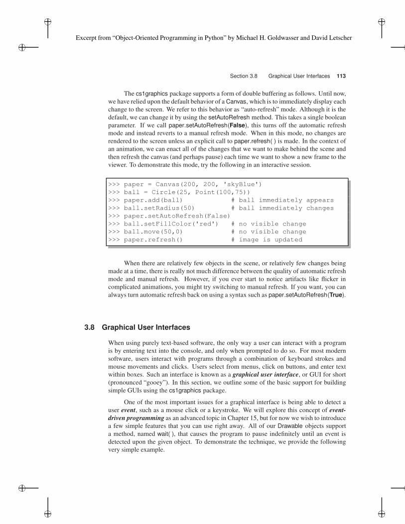
The cs1graphics package supports a form of double buffering as follows. Until now,

we have relied upon the default behavior of a Canvas, which is to immediately display each

change to the screen. We refer to this behavior as “auto-refresh” mode. Although it is the

default, we can change it by using the setAutoRefresh method. This takes a single boolean

parameter. If we call paper.setAutoRefresh(False), this turns off the automatic refresh

mode and instead reverts to a manual refresh mode. When in this mode, no changes are

rendered to the screen unless an explicit call to paper.refresh( ) is made. In the context of

an animation, we can enact all of the changes that we want to make behind the scene and

then refresh the canvas (and perhaps pause) each time we want to show a new frame to the

viewer. To demonstrate this mode, try the following in an interactive session.

>>> paper = Canvas(200, 200, 'skyBlue')

>>> ball = Circle(25, Point(100,75))

>>> paper.add(ball) # ball immediately appears

>>> ball.setRadius(50) # ball immediately changes

>>> paper.setAutoRefresh(False)

>>> ball.setFillColor('red') # no visible change

>>> ball.move(50,0) # no visible change

>>> paper.refresh() # image is updated

When there are relatively few objects in the scene, or relatively few changes being

made at a time, there is really not much difference between the quality of automatic refresh

mode and manual refresh. However, if you ever start to notice artifacts like flicker in

complicated animations, you might try switching to manual refresh. If you want, you can

always turn automatic refresh back on using a syntax such as paper.setAutoRefresh(True).

3.8 Graphical User Interfaces

When using purely text-based software, the only way a user can interact with a program

is by entering text into the console, and only when prompted to do so. For most modern

software, users interact with programs through a combination of keyboard strokes and

mouse movements and clicks. Users select from menus, click on buttons, and enter text

within boxes. Such an interface is known as a graphical user interface, or GUI for short

(pronounced “gooey”). In this section, we outline some of the basic support for building

simple GUIs using the cs1graphics package.

One of the most important issues for a graphical interface is being able to detect a

user event, such as a mouse click or a keystroke. We will explore this concept of event-

driven programming as an advanced topic in Chapter 15, but for now we wish to introduce

a few simple features that you can use right away. All of our Drawable objects support

a method, named wait( ), that causes the program to pause indefinitely until an event is

detected upon the given object. To demonstrate the technique, we provide the following

very simple example.



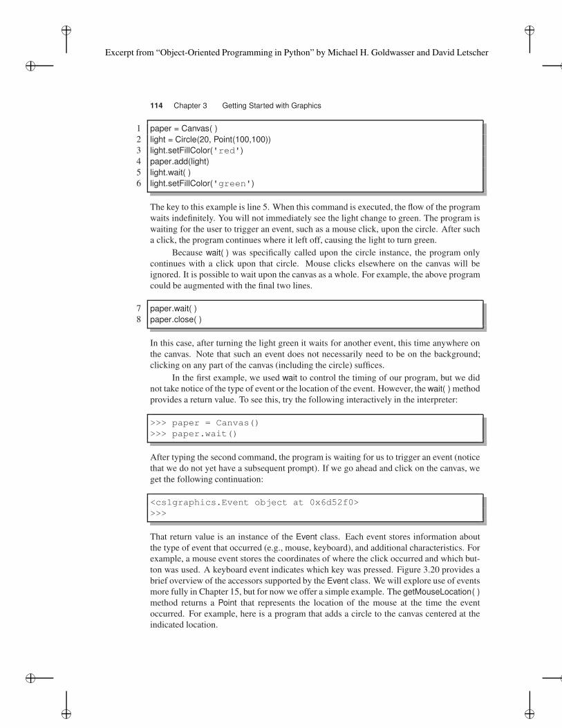
1 paper = Canvas( )

2 light = Circle(20, Point(100,100))

3 light.setFillColor('red')

4 paper.add(light)

5 light.wait( )

6 light.setFillColor('green')

The key to this example is line 5. When this command is executed, the flow of the program

waits indefinitely. You will not immediately see the light change to green. The program is

waiting for the user to trigger an event, such as a mouse click, upon the circle. After such

a click, the program continues where it left off, causing the light to turn green.

Because wait( ) was specifically called upon the circle instance, the program only

continues with a click upon that circle. Mouse clicks elsewhere on the canvas will be

ignored. It is possible to wait upon the canvas as a whole. For example, the above program

could be augmented with the final two lines.

7 paper.wait( )

8 paper.close( )

In this case, after turning the light green it waits for another event, this time anywhere on

the canvas. Note that such an event does not necessarily need to be on the background;

clicking on any part of the canvas (including the circle) suffices.

In the first example, we used wait to control the timing of our program, but we did

not take notice of the type of event or the location of the event. However, the wait( ) method

provides a return value. To see this, try the following interactively in the interpreter:

>>> paper = Canvas()

>>> paper.wait()

After typing the second command, the program is waiting for us to trigger an event (notice

that we do not yet have a subsequent prompt). If we go ahead and click on the canvas, we

get the following continuation:

<cs1graphics.Event object at 0x6d52f0>

>>>

That return value is an instance of the Event class. Each event stores information about

the type of event that occurred (e.g., mouse, keyboard), and additional characteristics. For

example, a mouse event stores the coordinates of where the click occurred and which but-

ton was used. A keyboard event indicates which key was pressed. Figure 3.20 provides a

brief overview of the accessors supported by the Event class. We will explore use of events

more fully in Chapter 15, but for now we offer a simple example. The getMouseLocation( )

method returns a Point that represents the location of the mouse at the time the event

occurred. For example, here is a program that adds a circle to the canvas centered at the

indicated location.


Section 3.8 Graphical User Interfaces 115

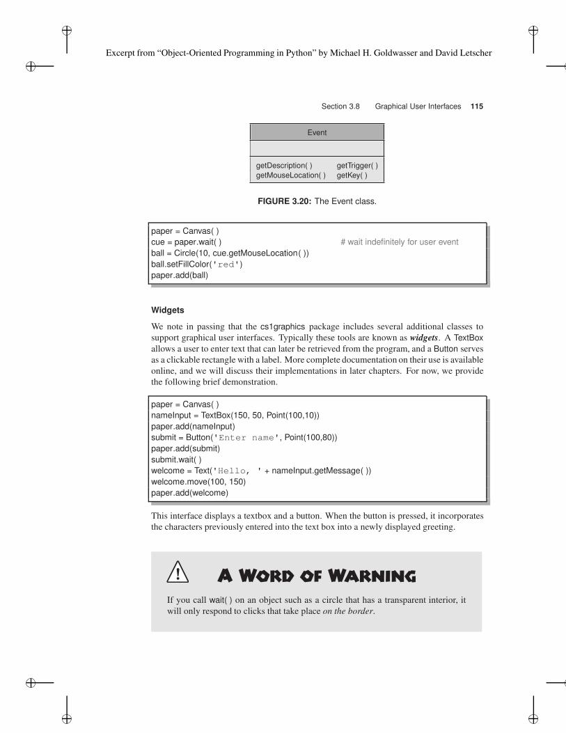
Event

getDescription( ) getTrigger( )

getMouseLocation( ) getKey( )

FIGURE 3.20: The Event class.

paper = Canvas( )

cue = paper.wait( ) # wait indefinitely for user event

ball = Circle(10, cue.getMouseLocation( ))

ball.setFillColor('red')

paper.add(ball)

Widgets

We note in passing that the cs1graphics package includes several additional classes to

support graphical user interfaces. Typically these tools are known as widgets. A TextBox

allows a user to enter text that can later be retrieved from the program, and a Button serves

as a clickable rectangle with a label. More complete documentation on their use is available

online, and we will discuss their implementations in later chapters. For now, we provide

the following brief demonstration.

paper = Canvas( )

nameInput = TextBox(150, 50, Point(100,10))

paper.add(nameInput)

submit = Button('Enter name', Point(100,80))

paper.add(submit)

submit.wait( )

welcome = Text('Hello, ' + nameInput.getMessage( ))

welcome.move(100, 150)

paper.add(welcome)

This interface displays a textbox and a button. When the button is pressed, it incorporates

the characters previously entered into the text box into a newly displayed greeting.

If you call wait( ) on an object such as a circle that has a transparent interior, it

will only respond to clicks that take place on the border.



Click target to fire an arrow Click target to fire an arrow

Click target to fire an arrow Good shooting!

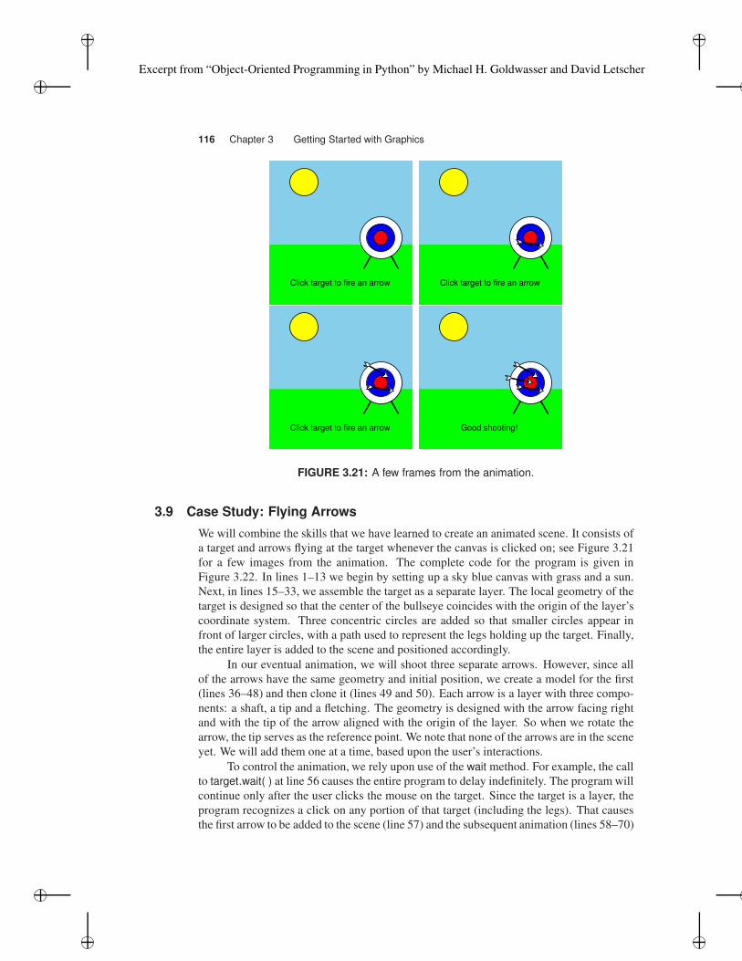
FIGURE 3.21: A few frames from the animation.

3.9 Case Study: Flying Arrows

We will combine the skills that we have learned to create an animated scene. It consists of

a target and arrows flying at the target whenever the canvas is clicked on; see Figure 3.21

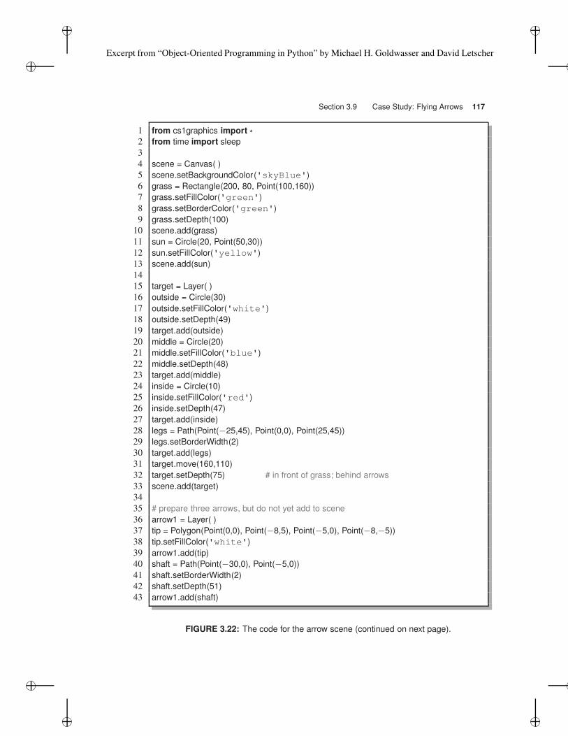
for a few images from the animation. The complete code for the program is given in

Figure 3.22. In lines 1–13 we begin by setting up a sky blue canvas with grass and a sun.

Next, in lines 15–33, we assemble the target as a separate layer. The local geometry of the

target is designed so that the center of the bullseye coincides with the origin of the layer’s

coordinate system. Three concentric circles are added so that smaller circles appear in

front of larger circles, with a path used to represent the legs holding up the target. Finally,

the entire layer is added to the scene and positioned accordingly.

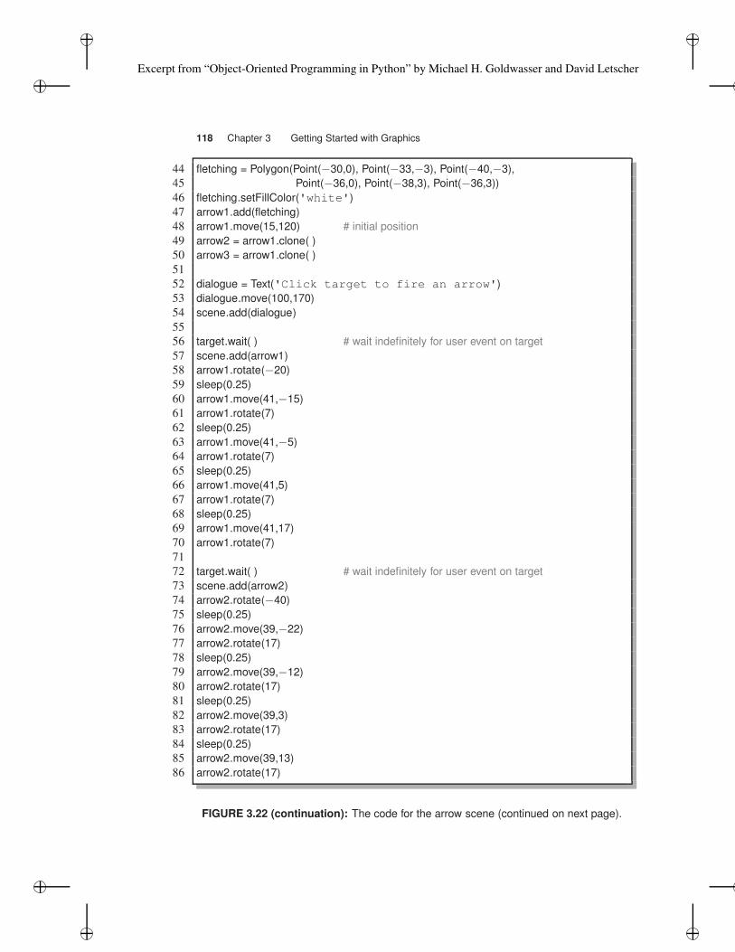
In our eventual animation, we will shoot three separate arrows. However, since all

of the arrows have the same geometry and initial position, we create a model for the first

(lines 36–48) and then clone it (lines 49 and 50). Each arrow is a layer with three compo-

nents: a shaft, a tip and a fletching. The geometry is designed with the arrow facing right

and with the tip of the arrow aligned with the origin of the layer. So when we rotate the

arrow, the tip serves as the reference point. We note that none of the arrows are in the scene

yet. We will add them one at a time, based upon the user’s interactions.

To control the animation, we rely upon use of the wait method. For example, the call

to target.wait( ) at line 56 causes the entire program to delay indefinitely. The program will

continue only after the user clicks the mouse on the target. Since the target is a layer, the

program recognizes a click on any portion of that target (including the legs). That causes

the first arrow to be added to the scene (line 57) and the subsequent animation (lines 58–70)


Section 3.9 Case Study: Flying Arrows 117

1 from cs1graphics import *2 from time import sleep

3

4 scene = Canvas( )

5 scene.setBackgroundColor('skyBlue')

6 grass = Rectangle(200, 80, Point(100,160))

7 grass.setFillColor('green')

8 grass.setBorderColor('green')

9 grass.setDepth(100)

10 scene.add(grass)

11 sun = Circle(20, Point(50,30))

12 sun.setFillColor('yellow')

13 scene.add(sun)

14

15 target = Layer( )

16 outside = Circle(30)

17 outside.setFillColor('white')

18 outside.setDepth(49)

19 target.add(outside)

20 middle = Circle(20)

21 middle.setFillColor('blue')

22 middle.setDepth(48)

23 target.add(middle)

24 inside = Circle(10)

25 inside.setFillColor('red')

26 inside.setDepth(47)

27 target.add(inside)

28 legs = Path(Point(−25,45), Point(0,0), Point(25,45))

29 legs.setBorderWidth(2)

30 target.add(legs)

31 target.move(160,110)

32 target.setDepth(75) # in front of grass; behind arrows

33 scene.add(target)

34

35 # prepare three arrows, but do not yet add to scene

36 arrow1 = Layer( )

37 tip = Polygon(Point(0,0), Point(−8,5), Point(−5,0), Point(−8,−5))

38 tip.setFillColor('white')

39 arrow1.add(tip)

40 shaft = Path(Point(−30,0), Point(−5,0))

41 shaft.setBorderWidth(2)

42 shaft.setDepth(51)

43 arrow1.add(shaft)

FIGURE 3.22: The code for the arrow scene (continued on next page).



44 fletching = Polygon(Point(−30,0), Point(−33,−3), Point(−40,−3),

45 Point(−36,0), Point(−38,3), Point(−36,3))

46 fletching.setFillColor('white')

47 arrow1.add(fletching)

48 arrow1.move(15,120) # initial position

49 arrow2 = arrow1.clone( )

50 arrow3 = arrow1.clone( )

51

52 dialogue = Text('Click target to fire an arrow')

53 dialogue.move(100,170)

54 scene.add(dialogue)

55

56 target.wait( ) # wait indefinitely for user event on target

57 scene.add(arrow1)

58 arrow1.rotate(−20)

59 sleep(0.25)

60 arrow1.move(41,−15)

61 arrow1.rotate(7)

62 sleep(0.25)


64 arrow1.rotate(7)

65 sleep(0.25)

66 arrow1.move(41,5)

67 arrow1.rotate(7)

68 sleep(0.25)


70 arrow1.rotate(7)

71

72 target.wait( ) # wait indefinitely for user event on target



75 sleep(0.25)


77 arrow2.rotate(17)

78 sleep(0.25)



81 sleep(0.25)



84 sleep(0.25)



FIGURE 3.22 (continuation): The code for the arrow scene (continued on next page).


Section 3.9 Case Study: Flying Arrows 119



89 sleep(0.25)



92 sleep(0.25)



95 sleep(0.25)



98 sleep(0.25)



101 dialogue.setMessage('Good shooting!')

102

103 scene.wait( ) # wait for user event anywhere on canvas

104 scene.close( )

FIGURE 3.22 (continuation): The code for the arrow scene.

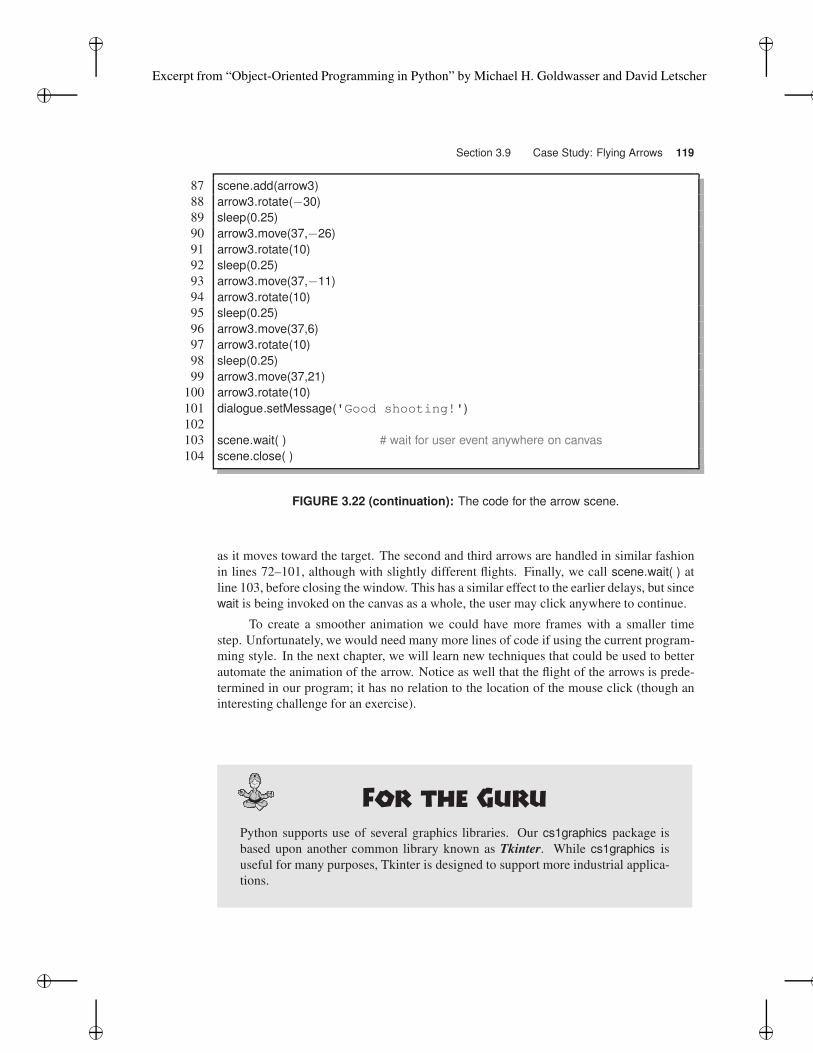
as it moves toward the target. The second and third arrows are handled in similar fashion

in lines 72–101, although with slightly different flights. Finally, we call scene.wait( ) at

line 103, before closing the window. This has a similar effect to the earlier delays, but since

wait is being invoked on the canvas as a whole, the user may click anywhere to continue.

To create a smoother animation we could have more frames with a smaller time

step. Unfortunately, we would need many more lines of code if using the current program-

ming style. In the next chapter, we will learn new techniques that could be used to better

automate the animation of the arrow. Notice as well that the flight of the arrows is prede-

termined in our program; it has no relation to the location of the mouse click (though an

interesting challenge for an exercise).

Python supports use of several graphics libraries. Our cs1graphics package is

based upon another common library known as Tkinter. While cs1graphics is

useful for many purposes, Tkinter is designed to support more industrial applica-

tions.



3.10 Chapter Review

3.10.1 Key Points

Graphics Primitives

• Creating a Canvas instance constructs a window. Various objects can be visualized by

calling the add method of the canvas.

• The window for a canvas does not close unless the user manually closes the window

through the operating system or the close method of the canvas is called.

• Coordinates are measured from the top left corner of the window. The x-coordinate speci-

fies the number of pixels to the right of this point and the y-coordinate specifies the number

of pixels below this point.

• Only Drawable objects can be added to a canvas.

Modifying Drawable Objects

• There are mutators to change the location, color, border color, position, and other features

for each drawable object.

• A drawable object can be rotated, scaled, or flipped relative to its reference point. This

reference point can be reconfigured using the adjustReference member function.

Depths

• When two or more drawable objects overlap on a canvas, the relative ordering of those

objects is determined according to their specified depth attribute. Shapes with smaller

depths are drawn in front of those with larger depths.

Layers

• A Layer represents a collection of objects that is treated as a single shape. They layer can

be added, moved, rotated or scaled, just as with any other Drawable instance.

• Depths of objects within a layer only affects how the objects in the layer appear relative to

each other. The depth of the layer controls whether all the shapes in that layer appears in

front or behind objects that are not part of the layer.

Animation

• A time delay for an animation can be achieved by calling the sleep function imported from

the time module.

• Flicker can be reduced in an animation by turning auto-refresh off for the canvas and calling

refresh each time you want the canvas’s image rendered to the screen.

Events

• Calling the wait( ) method of the Canvas class causes the program to wait indefinitely until

the user triggers an event on the window, such as a mouse click or keypress.

• Calling the wait( ) method on an individual drawable object waits until the user triggers

and event specifically upon that particular object.

• The wait( ) function returns an Event instance that contains information about which mouse

button or key was pressed, and the cursor location at that time.


Section 3.10 Chapter Review 121

3.10.2 Glossary

canvas A graphics window on which objects can be drawn.

clone A copy of an object.

double buffering A technique for avoiding flicker in animation by computing incremen-

tal changes internally before displaying a new image to the viewer.

event An external stimulus on a program, such as a user’s mouse click.

event-driven programming A style in which a program passively waits for external

events to occur, responding appropriately to those events as needed.

graphical user interface (GUI) A design allowing a user to interact with software

through a combination of mouse movements, clicks, and keyboard commands.

pixel The smallest displayable element in a digital picture.

reference point A particular location for a cs1graphics.Drawable instance that is used

when determining the placement of the object upon a canvas’s coordinate system.

The reference point remains fixed when the object is scaled, rotated, or flipped.

RGB value A form for specifying a color as a triple of integers representing the intensity

of the red, green, and blue components of the color. Typically, each color is measured

on a scale from 0 to 255.

widget An object that serves a particular purpose in a graphical user interface.

3.10.3 Exercises

Graphics Primitives

Practice 3.1: The following code fragment has a single error in it. Fix it.

1 from cs1graphics import *2 screen = Canvas( )

3 disk = Circle( )

4 disk.setFillColor('red')

5 disk.add(screen)

Practice 3.2: Write a program that draws a filled triangle near the middle of a canvas.

For Exercise 3.3 through Exercise 3.7, try to find the errors without using a computer. Then

try running them on the computer to help find the errors or confirm your answers.

Exercise 3.3: After starting Python, you immediately enter

can = Canvas(100,100)

Python reports an error with the last line saying

NameError : name 'Canvas' is not defined

What did you do wrong? How do you fix it?



Exercise 3.4: Assuming that you have already created an instance of the Square class

called sq, what’s wrong with the statement

sq.setFillColor(Red)

Give two different ways to fix this statement.

Exercise 3.5: Assuming that you have already successfully created a Canvas instance

called can, you enter the following to draw a blue circle centered in a red square:

sq = Square( )

sq.setSize(40)

sq.moveTo(30,30)

sq.setFillColor('Red')

can.add(sq)

cir = Circle( )

cir.moveTo(50,50)

cir.setRadius(15)

cir.setFillColor('Blue')

can.add(cir)

But the circle never appears. What’s wrong with the above program? Edit the pro-

gram so it works as desired.

Exercise 3.6: Consider the following:

can = Canvas(200,150)

rect = Rectangle( )

rect.setWidth(50)

rect.setHeight(75)

rect.moveTo(25,25)

rect = Rectangle( )

rect.setWidth(100)

rect.setHeight(25)

can.add(rect)

can.add(rect)

Only one rectangle appears? Why? How would you get two different rectangles to

show up? (There are several ways to fix this.)


Section 3.10 Chapter Review 123

Layers

Exercise 3.7: The following runs but does not display anything. What is wrong?

can = Canvas( )

lay = Layer( )

sq = Square( )

lay.add(sq)

Exercise 3.8: Use the Layer class of the graphics library to create a pine tree. Make copies

of the tree and use it to draw a forest of pine trees.

Exercise 3.9: Redo the smiley face described in the chapter as a layer. Test the code by

rotating and scaling the layer and ensuring the face does not get distorted.

Exercise 3.10: Create an airplane as a layer and animate it flying across the screen and

doing a loop. Hint: think carefully about the placement of the reference point.

Graphics Scenes

Exercise 3.11: Use the graphics library to create a picture of your favorite animal with an

appropriate background scene.

Exercise 3.12: Use the graphics library to draw an analog clock face with numbers at the

appropriate locations and an hour and minute hand.

Events

Exercise 3.13: Display the text "Click Me" centered in a graphics canvas. When the user

clicks on the text, close the canvas.

Exercise 3.14: Create a program that draws a traditional traffic signal with three lights

(green, yellow, and red). In the initial configuration, the green light should be on,

but the yellow and red off (that is, black). When the user clicks the mouse on the

signal, turn the green off and the yellow on; when the user clicks again, turn the

yellow off and the red on.

Exercise 3.15: Write a program that displays a Text object graphically and adds characters

typed on the keyboard to the message on the canvas.

Exercise 3.16: Write a program that allows the user to draw a path between five points,

with each point specified by a mouse click on the canvas. As each successive click

is received, display the most recent segment on the canvas.

Projects

Exercise 3.17: Use the graphics library to draw an analog clock face with hour, minute,

and second hands. Use the datetime module to start the clock at the current time and

animate the clock so that it advances once per second.

Exercise 3.18: Write a game of Tic-tac-toe using a graphical interface. The program

should draw the initial board, and then each time the mouse is clicked, determine

the appropriate square of the game board for drawing an X or an O. You may allow

the game to continue for each of the nine turns. (As a bonus, read ahead to Chapter 4

and figure out how to stop the game once a player wins.)

Exercise 3.19: Think of your own cool project and have fun with it.

object-oriented programming in python - cs1graphics

Documents