obAnalytics GuidePhilip Stubbings

2016-11-11

Contents

Overview 1

Recommended environment settings . . . . . . . . . . . . . . . . . . . . . . . . . . . . . . . . . . . 1

Loading data 2

Expected csv schema . . . . . . . . . . . . . . . . . . . . . . . . . . . . . . . . . . . . . . . . . . . . 2

Preprocessed example data . . . . . . . . . . . . . . . . . . . . . . . . . . . . . . . . . . . . . . . . 2

Visualisation 6

Order book shape . . . . . . . . . . . . . . . . . . . . . . . . . . . . . . . . . . . . . . . . . . . . . 7

Price level volume . . . . . . . . . . . . . . . . . . . . . . . . . . . . . . . . . . . . . . . . . . . . . 7

Liquidity . . . . . . . . . . . . . . . . . . . . . . . . . . . . . . . . . . . . . . . . . . . . . . . . . . 13

Order cancellations . . . . . . . . . . . . . . . . . . . . . . . . . . . . . . . . . . . . . . . . . . . . . 15

Analysis 18

Order book reconstruction . . . . . . . . . . . . . . . . . . . . . . . . . . . . . . . . . . . . . . . . . 18

Market impacts . . . . . . . . . . . . . . . . . . . . . . . . . . . . . . . . . . . . . . . . . . . . . . . 18

Overview

obAnalytics is an R package intended for visualisation and analysis of limit order data.

This guide is structured as an end-to-end walk-through and is intended to demonstrate the main features andfunctionality of the package.

Recommended environment settings

Due to the large number of columns in the example data, it is recommended to set the display width to makethe most use of the display. It is also recommended to set digits.secs=3 and scipen=999 in order to displaytimestamps and fractions nicely. This can be achieved as follows:

max.cols <- Sys.getenv("COLUMNS")options(width=if(max.cols != "") max.cols else 80, scipen=999, digits.secs=3)

1

Loading data

The main focus of this package is reconstruction of a limit order book. The processData function will performdata processing based on a supplied CSV file, the format of which is defined in the Expected csv schemasection.

The data processing consists of a number of stages:

1. Cleaning of duplicate and erroneous data.

2. Identification of sequential event relationships.

3. Inference of trade events via order-matching.

4. Inference of order types (limit vs market).

5. Construction of volume by price level series.

6. Construction of order book summary statistics.

Limit order events are related to one another by volume deltas (the change in volume for a limit order).To simulate a matching-engine, and thus determine directional trade data, volume deltas from both sidesof the limit order book are ordered by time, yielding a sequence alignment problem, to which the theNeedleman-Wunsch algorithm has been applied.

# load and process example csv data from the package inst/extdata directory.csv.file <- system.file("extdata", "orders.csv.xz", package="obAnalytics")lob.data <- processData(csv.file)

Expected csv schema

The CSV file is expected to contain 7 columns:

Table 1: Expected CSV schema.

Column name Descriptionid Numeric limit order unique identifier.

timestamp Time in milliseconds when event received locally.exchange.timestamp Time in milliseconds when order first created on the exchange.

price Price level of order event.volume Remaining order volume.action Event action describes the limit order lifecycle. One of: created,

modified, deleted.direction Side of order book. On of: bid or ask.

Preprocessed example data

For illustrative purposes, the package contains a sample of preprocessed data. The data, taken from theBitstamp (bitcoin) exchange on 2015-05-01, consists of 50,393 limit order events and 482 trades occuringfrom midnight up until ~5am.

The sample data, which has been previously processed by the processData function, may be attached to theenvironment with the data() function:

2

data(lob.data)

The lob.data object is a list containing four data.frames.

Table 2: lob.data summary.

data.frame Summaryevents Limit order events.trades Inferred trades (executions).depth Order book price level depth through time.

depth.summary Limit order book summary statistics.

The contents of which are briefly discussed in the following sections.

Events

The events data.frame contains the lifecycle of limit orders and makes up the core data of the obAnalyticspackage. Each row corresponds to a single limit order action, of which three types are possible.

Table 3: Possible limit order actions.

Event action Meaningcreated The order is created with a specified amount of volume and a limit price.changed The order has been partially filled. On each modification, the remaining volume will

decrease.deleted The order may be deleted at the request of the trader or, in the event that the order

has been completely filled, deleted by the exchange. An order deleted by theexchange as a result of being filled will have 0 remaining volume at time of deletion.

In addition to the event action type, a row consists of a number of attributes relating to the lifecycle of alimit order.

Table 4: Limit order event attributes.

Attribute Meaningevent.id Event Id.

id Limit Order Id.timestamp Local event timestamp (local time the event was observed).

exchange.timestamp Exchange order creation time.price Limit order price level.

volume Remaining limit order volume.action Event action: created, changed, deleted. (as described above).

direction Order book side: bid, ask.fill For changed or deleted events, indicates the change in volume between

this event and the last.matching.event Matching event.id if this event is part of a trade. NA otherwise.

type Limit order type (see Event types below.)

3

Attribute Meaningaggressiveness.bps The distance of the order from the edge of the book in Basis Points

(BPS). If an order is placed exactly at the best bid/ask queue, this valuewill be 0. If placed behind the best bid/ask, the value will be negative. Apositive value is indicative of a innovative order: The order was placedinside the bid/ask spread, which would result in the change to themarket midprice.

An individual limit order (referenced by the id attribute) may be of six different types, all of which havebeen classified by onAnalytics.

Table 5: Order types.

Limit order type Meaningunknown It was not possible to infer the order type given the available data.

flashed-limit Order was created then subsequently deleted. 96% of example data. Thesetypes of orders are also referred to as fleeting orders in the literature.

resting-limit Order was created and left in order book indefinitely until filled.market-limit Order was partially filled before landing in the order book at it’s limit price.

This may happen when the limit order crosses the book because, in the case ofa bid order, it’s price is >= the current best ask. However there is not enoughvolume between the current best ask and the order limit price to fill the order’svolume completely.

market Order was completely filled and did not come to rest in the order book.Similarly to a market-limit, the market order crosses the order book. However,it’s volume is filled before reaching it’s limit price. Both market-limit andmarket orders are referred to as marketable limit orders in the literature.

pacman A limit-price modified in situ (exchange algorithmic order). The example datacontains a number of these order types. They occur when a limit order’s priceattribute is updated. In the example data, this occurs from a special order typeoffered by the exchange which, in the case of a bid, will peg the limit price tothe best ask once per second until the order has been filled.

The following table demonstrates a small snapshot (1 second) of event data. Some of the attributes havebeen omitted or renamed for readability.

one.sec <- with(lob.data, {events[events$timestamp >= as.POSIXct("2015-05-01 04:55:10", tz="UTC") &

events$timestamp <= as.POSIXct("2015-05-01 04:55:11", tz="UTC"), ]})one.sec$volume <- one.sec$volume*10^-8one.sec$fill <- one.sec$fill*10^-8one.sec$aggressiveness.bps <- round(one.sec$aggressiveness.bps, 2)one.sec <- one.sec[, c("event.id", "id", "price", "volume", "action",

"direction", "fill", "matching.event", "type", "aggressiveness.bps")]colnames(one.sec) <- c(c("event.id", "id", "price", "vol", "action", "dir",

"fill", "match", "type", "agg"))print(one.sec, row.names=F)

4

event.id id price vol action dir fill match type agg48258 65619043 235.84 0.000000 deleted ask 1.6379919 49021 market-limit NA48443 65619136 235.98 0.000000 deleted ask 0.2118824 49022 resting-limit -6.3648617 65619223 237.12 20.762160 deleted ask 0.0000000 NA flashed-limit -47.0348879 65619359 236.18 15.988592 deleted ask 0.0000000 NA flashed-limit -7.2048997 65619419 235.83 0.000000 deleted ask 1.8498742 NA unknown NA49001 65619421 236.01 15.435748 changed ask 6.6832516 49023 resting-limit NA49020 65619430 236.05 8.533126 changed bid 1.8498742 NA market NA49021 65619430 236.05 6.895134 changed bid 1.6379919 48258 market NA49022 65619430 236.05 6.683252 changed bid 0.2118824 48443 market NA49023 65619430 236.05 0.000000 deleted bid 6.6832516 49001 market NA49024 65619431 235.06 13.200000 created bid 0.0000000 NA resting-limit -28.8549027 65619432 236.03 13.200000 created ask 0.0000000 NA flashed-limit -0.8549029 65619433 233.71 8.665815 created bid 0.0000000 NA flashed-limit -86.1149030 65619433 233.71 8.665815 deleted bid 0.0000000 NA flashed-limit -86.1149031 65619434 236.94 22.749000 created ask 0.0000000 NA flashed-limit -39.41

Trades

The package automatically infers execution/trade events from the provided limit order data.

The trades data.frame contains a log of all executions ordered by local timestamp.

In addition to the usual timestamp, price and volume information, each row also contains the trade direction(buyer or seller initiated) and maker/taker limit order ids.

The maker/taker event and limit order ids can be used to group trades into market impacts - An example ofwhich will be demonstrated later in this guide.

trades.ex <- tail(lob.data$trades, 10)trades.ex$volume <- round(trades.ex$volume*10^-8, 2)print(trades.ex, row.names=F)

timestamp price volume direction maker.event.id taker.event.id maker taker2015-05-01 04:59:27.503 235.73 0.01 buy 49630 49777 65619731 656198062015-05-01 04:59:27.532 235.79 0.02 buy 49672 49778 65619752 656198062015-05-01 04:59:41.568 235.77 0.02 buy 49802 49821 65619818 656198262015-05-01 04:59:55.877 235.77 0.02 buy 49803 49871 65619818 656198512015-05-01 04:59:59.217 235.77 0.38 buy 49804 49877 65619818 656198542015-05-01 05:00:08.361 235.77 0.12 sell 49878 49894 65619854 656198622015-05-01 05:00:08.395 235.58 0.21 sell 49406 49895 65619615 656198622015-05-01 05:00:08.424 235.01 0.07 sell 46221 49896 65618028 656198622015-05-01 05:00:10.108 235.79 0.02 buy 49816 49900 65619824 656198642015-05-01 05:03:13.566 235.45 0.05 sell 49992 50255 65619912 65620048

Each row, representing a single trade, consists of the following attributes:

Table 8: Trade data attributes.

Attribute Meaningtimestamp Local event timestamp.

5

Attribute Meaningprice Price at which the trade occurred.

volume Amount of traded volume.direction The trade direction: buy or sell.

maker.event.id Corresponding market making event id in events data.frame.taker.event.id Corresponding market taking event id in events data.frame.

maker Id of the market making limit order in events data.frame.taker Id of the market taking limit order in events data.frame.

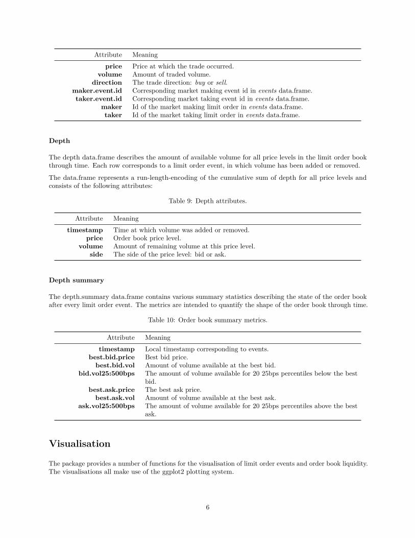
Depth

The depth data.frame describes the amount of available volume for all price levels in the limit order bookthrough time. Each row corresponds to a limit order event, in which volume has been added or removed.

The data.frame represents a run-length-encoding of the cumulative sum of depth for all price levels andconsists of the following attributes:

Table 9: Depth attributes.

Attribute Meaningtimestamp Time at which volume was added or removed.

price Order book price level.volume Amount of remaining volume at this price level.

side The side of the price level: bid or ask.

Depth summary

The depth.summary data.frame contains various summary statistics describing the state of the order bookafter every limit order event. The metrics are intended to quantify the shape of the order book through time.

Table 10: Order book summary metrics.

Attribute Meaningtimestamp Local timestamp corresponding to events.

best.bid.price Best bid price.best.bid.vol Amount of volume available at the best bid.

bid.vol25:500bps The amount of volume available for 20 25bps percentiles below the bestbid.

best.ask.price The best ask price.best.ask.vol Amount of volume available at the best ask.

ask.vol25:500bps The amount of volume available for 20 25bps percentiles above the bestask.

Visualisation

The package provides a number of functions for the visualisation of limit order events and order book liquidity.The visualisations all make use of the ggplot2 plotting system.

6

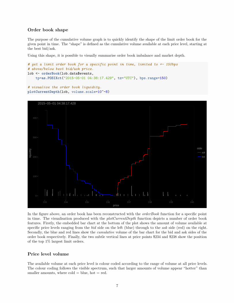
Order book shape

The purpose of the cumulative volume graph is to quickly identify the shape of the limit order book for thegiven point in time. The “shape” is defined as the cumulative volume available at each price level, starting atthe best bid/ask.

Using this shape, it is possible to visually summarise order book imbalance and market depth.

# get a limit order book for a specific point in time, limited to +- 150bps# above/below best bid/ask price.lob <- orderBook(lob.data$events,

tp=as.POSIXct("2015-05-01 04:38:17.429", tz="UTC"), bps.range=150)

# visualise the order book liquidity.plotCurrentDepth(lob, volume.scale=10^-8)

0

100

200

300

400

233 234 235 236 237 238 239 240

price

liqui

dity side

ask

bid

2015−05−01 04:38:17.428

In the figure above, an order book has been reconstructed with the orderBook function for a specific pointin time. The visualisation produced with the plotCurrentDepth function depicts a number of order bookfeatures. Firstly, the embedded bar chart at the bottom of the plot shows the amount of volume available atspecific price levels ranging from the bid side on the left (blue) through to the ask side (red) on the right.Secondly, the blue and red lines show the cumulative volume of the bar chart for the bid and ask sides of theorder book respectively. Finally, the two subtle vertical lines at price points $234 and $238 show the positionof the top 1% largest limit orders.

Price level volume

The available volume at each price level is colour coded according to the range of volume at all price levels.The colour coding follows the visible spectrum, such that larger amounts of volume appear “hotter” thansmaller amounts, where cold = blue, hot = red.

7

Since the distribution of limit order size exponentially decays, it can be difficult to visually differentiate: mostvalues will appear to be blue. The function provides price, volume and a colour bias range to overcome this.

Setting col.bias to 0 will colour code volume on the logarithmic scale, while setting col.bias < 1 will “squash”the spectrum. For example, a uniform col.bias of 1 will result in 1/3 blue, 1/3 green, and 1/3 red appliedacross all volume - most values will be blue. Setting the col.bias to 0.5 will result in 1/7 blue, 2/7 green, 4/7red being applied such that there is greater differentiation amongst volume at smaller scales.

# plot all lob.data price level volume between $233 and $245 and overlay the# market midprice.spread <- getSpread(lob.data$depth.summary)plotPriceLevels(lob.data$depth, spread, price.from=233, price.to=245,

volume.scale=10^-8, col.bias=0.25, show.mp=T)

233.0

233.5

234.0

234.5

235.0

235.5

236.0

236.5

237.0

237.5

238.0

238.5

239.0

239.5

240.0

240.5

241.0

241.5

242.0

242.5

243.0

243.5

244.0

244.5

245.0

00:00 01:00 02:00 03:00 04:00 05:00

time

limit

pric

e

8.64966

123.327

volume

The above plot shows all price levels between $227 and $245 for ~5 hours of price level data with the marketmidprice indicated in white. The volume has been scaled down from Satoshi to Bitcoin for legibility (1 Bitcoin= 10ˆ8 Satoshi). Note the large sell/ask orders at $238 and $239 respectively.

Zooming into the same price level data, between 1am and 2am and providing trades data to the plot willshow trade executions. In the below plot which has been centred around the bid/ask spread, shows the pointsat which market sell (circular red) and buy (circular green) orders have been executed with respect to theorder book price levels.

# plot 1 hour of trades centred around the bid/ask spread.plotPriceLevels(lob.data$depth, trades=lob.data$trades,

price.from=236, price.to=237.75, volume.scale=10^-8, col.bias=0.2,start.time=as.POSIXct("2015-05-01 01:00:00.000", tz="UTC"),end.time=as.POSIXct("2015-05-01 02:00:00.000", tz="UTC"))

8

236.0

236.5

237.0

237.5

01:00 01:15 01:30 01:45 02:00

time

limit

pric

e

4.31605

75.8073

volume

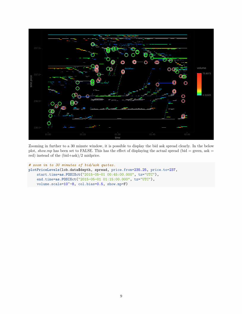
Zooming in further to a 30 minute window, it is possible to display the bid ask spread clearly. In the belowplot, show.mp has been set to FALSE. This has the effect of displaying the actual spread (bid = green, ask =red) instead of the (bid+ask)/2 midprice.

# zoom in to 30 minutes of bid/ask quotes.plotPriceLevels(lob.data$depth, spread, price.from=235.25, price.to=237,

start.time=as.POSIXct("2015-05-01 00:45:00.000", tz="UTC"),end.time=as.POSIXct("2015-05-01 01:15:00.000", tz="UTC"),volume.scale=10^-8, col.bias=0.5, show.mp=F)

9

235.5

236.0

236.5

237.0

00:50 01:00 01:10

time

limit

pric

e

3.7966

64.2360

volume

Zooming in, still further, to ~4 minutes of data focussed around the spread, shows (in this example) the bidrising and then dropping, while, by comparison, the ask price remains static.

This is a common pattern: 2 or more algorithms are competing to be ahead of each other. They both wish tobe at the best bid+1, resulting in a cyclic game of leapfrog until one of the competing algorithm withdraws,in which case the remaining algorithm “snaps” back to the next best bid (+1). This behavior results in asawtooth pattern which has been characterised by some as market- manipulation. It is simply an emergentresult of event driven limit order markets.

# zoom in to 4 minutes of bid/ask quotes.plotPriceLevels(lob.data$depth, spread, price.from=235.90, price.to=236.25,

start.time=as.POSIXct("2015-05-01 00:55:00.000", tz="UTC"),end.time=as.POSIXct("2015-05-01 00:59:00.000", tz="UTC"),volume.scale=10^-8, col.bias=0.5, show.mp=F)

10

236

00:55 00:56 00:57 00:58 00:59

time

limit

pric

e

3.7053

10.4573

volume

By filtering the price or volume range it is possible to observe the behavior of individual market participants.This is perhaps one of the most useful and interesting features of this tool.

In the below plot, the displayed price level volume has been restricted between 8.59 an 8.72 bitcoin, resultingin obvious display of an individual algo. Here, the algo. is most likely seeking value by placing limit ordersbelow the bid price waiting for a market impact in the hope of reversion by means of market resilience (therate at which market makers fill a void after a market impact).

plotPriceLevels(lob.data$depth, spread, price.from=232.5, price.to=237.5,volume.scale=10^-8, col.bias=1, show.mp=T,end.time=as.POSIXct("2015-05-01 01:30:00.000", tz="UTC"),volume.from=8.59, volume.to=8.72)

11

233.0

233.5

234.0

234.5

235.0

235.5

236.0

236.5

237.0

237.5

00:00 00:30 01:00 01:30

time

limit

pric

e

8.66013

8.71692

volume

Using the same volume filtering approach, the next plot shows the behaviour of an individual market makeroperating with a bid/ask spread limited between 3.63 and 3.83 bitcoin respectively. The rising bid prices attimes are due to the event driven “leapfrog” phenomenon discussed previously.

plotPriceLevels(lob.data$depth, price.from=235.65, price.to=237.65,volume.scale=10^-8, col.bias=1,start.time=as.POSIXct("2015-05-01 01:00:00.000", tz="UTC"),end.time=as.POSIXct("2015-05-01 03:00:00.000", tz="UTC"),volume.from=3.63, volume.to=3.83)

12

236.0

236.5

237.0

237.5

01:00 01:30 02:00 02:30 03:00

time

limit

pric

e

3.7159

3.82668

volume

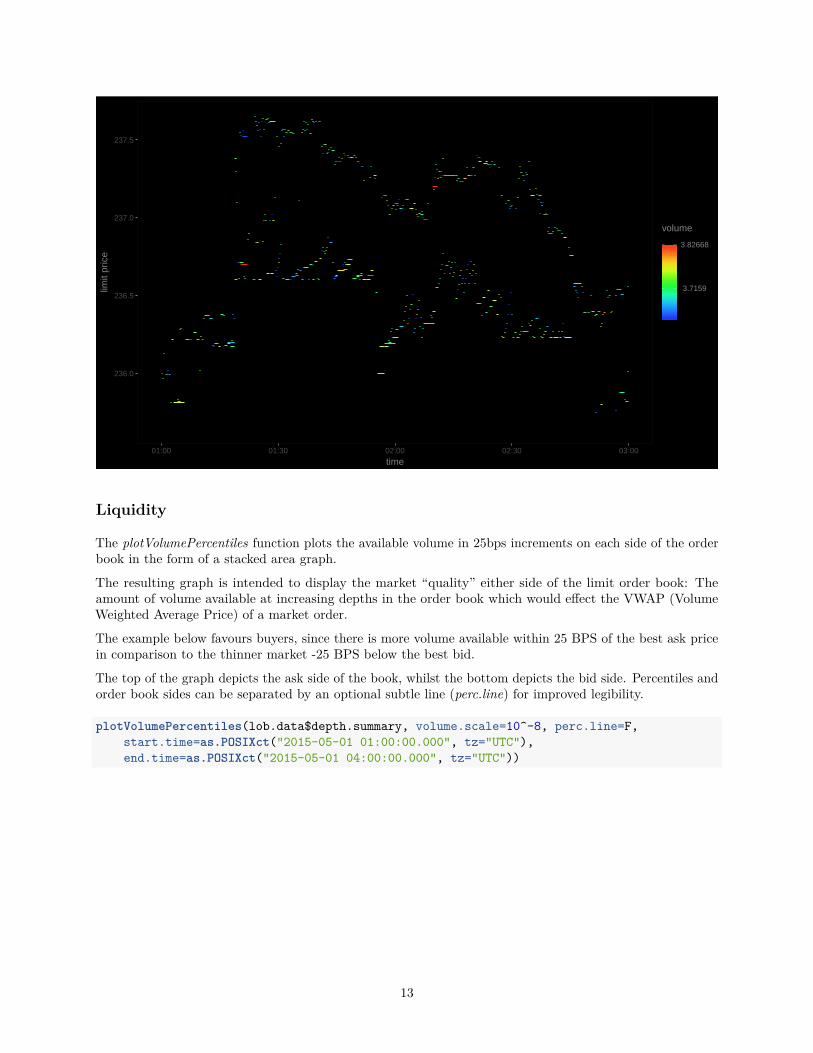
Liquidity

The plotVolumePercentiles function plots the available volume in 25bps increments on each side of the orderbook in the form of a stacked area graph.

The resulting graph is intended to display the market “quality” either side of the limit order book: Theamount of volume available at increasing depths in the order book which would effect the VWAP (VolumeWeighted Average Price) of a market order.

The example below favours buyers, since there is more volume available within 25 BPS of the best ask pricein comparison to the thinner market -25 BPS below the best bid.

The top of the graph depicts the ask side of the book, whilst the bottom depicts the bid side. Percentiles andorder book sides can be separated by an optional subtle line (perc.line) for improved legibility.

plotVolumePercentiles(lob.data$depth.summary, volume.scale=10^-8, perc.line=F,start.time=as.POSIXct("2015-05-01 01:00:00.000", tz="UTC"),end.time=as.POSIXct("2015-05-01 04:00:00.000", tz="UTC"))

13

−1000

−500

0

500

1000

01:00 02:00 03:00 04:00

time

liqui

dity

depth

+500bps

+450bps

+400bps

+350bps

+300bps

+250bps

+200bps

+150bps

+100bps

+050bps

−050bps

−100bps

−150bps

−200bps

−250bps

−300bps

−350bps

−400bps

−450bps

−500bps

Zooming in to a 5 minute window and enabling the percentile borders with (perc.line=FALSE), the amountof volume available at each 25 bps price level is exemplified.

# visualise 5 minutes of order book liquidity.# data will be aggregated to second-by-second resolution.plotVolumePercentiles(lob.data$depth.summary,

start.time=as.POSIXct("2015-05-01 04:30:00.000", tz="UTC"),end.time=as.POSIXct("2015-05-01 04:35:00.000", tz="UTC"),volume.scale=10^-8)

14

−1000

−500

0

500

1000

04:30 04:32 04:34

time

liqui

dity

depth

+500bps

+450bps

+400bps

+350bps

+300bps

+250bps

+200bps

+150bps

+100bps

+050bps

−050bps

−100bps

−150bps

−200bps

−250bps

−300bps

−350bps

−400bps

−450bps

−500bps

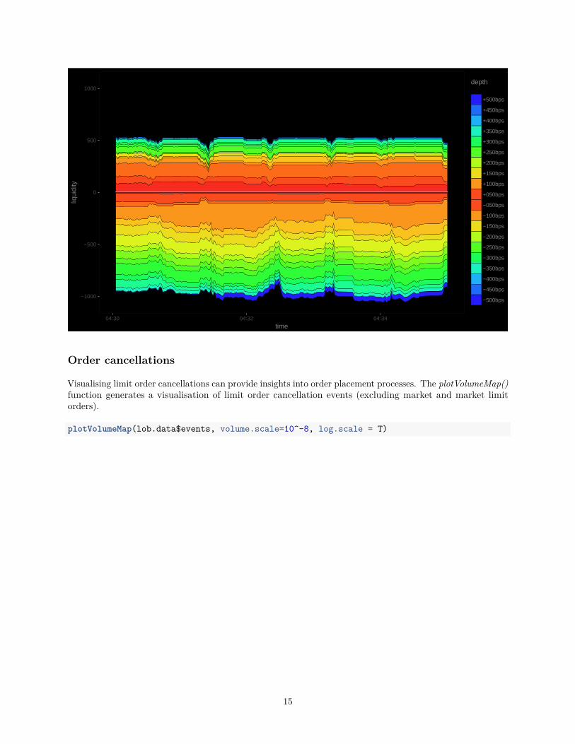
Order cancellations

Visualising limit order cancellations can provide insights into order placement processes. The plotVolumeMap()function generates a visualisation of limit order cancellation events (excluding market and market limitorders).

plotVolumeMap(lob.data$events, volume.scale=10^-8, log.scale = T)

15

0.37

7.39

148.41

00:00 01:00 02:00 03:00 04:00 05:00

time

canc

elle

d vo

lum

e

direction

bid

ask

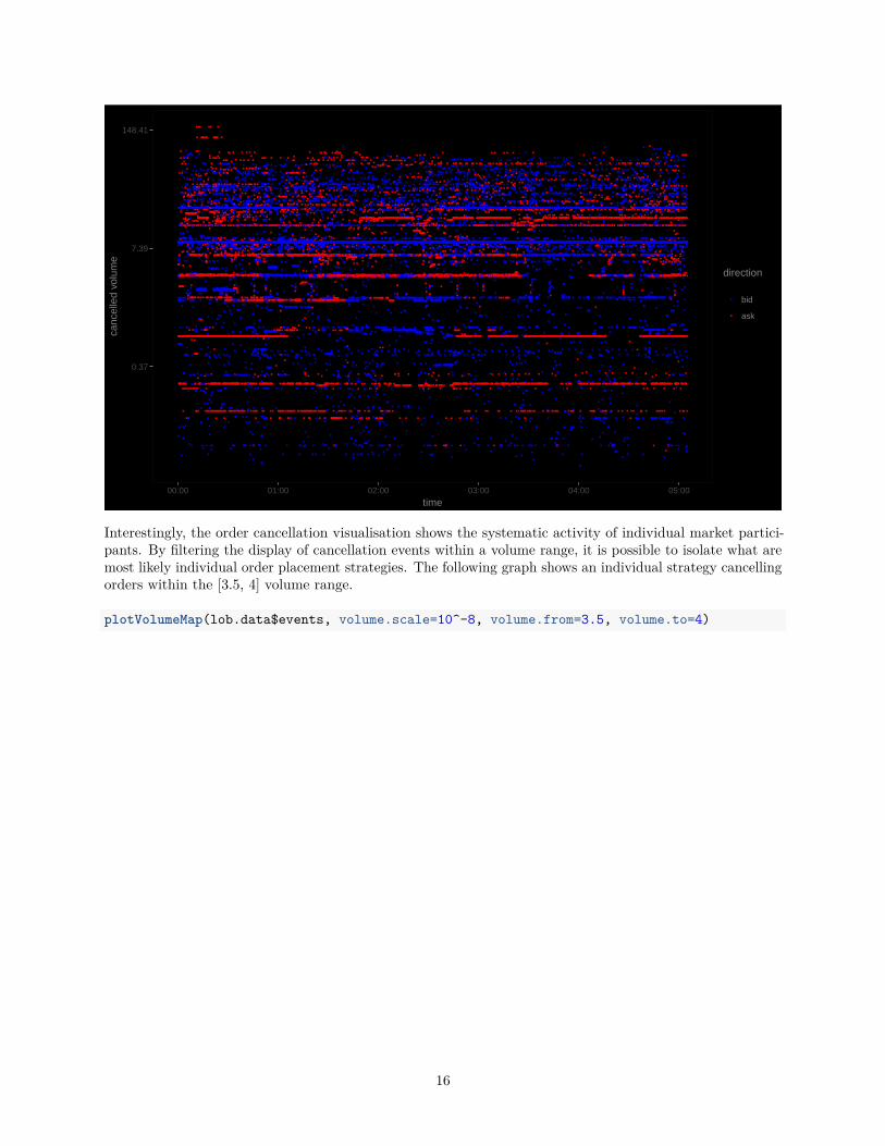
Interestingly, the order cancellation visualisation shows the systematic activity of individual market partici-pants. By filtering the display of cancellation events within a volume range, it is possible to isolate what aremost likely individual order placement strategies. The following graph shows an individual strategy cancellingorders within the [3.5, 4] volume range.

plotVolumeMap(lob.data$events, volume.scale=10^-8, volume.from=3.5, volume.to=4)

16

3.50

3.60

3.70

3.80

3.90

4.00

00:00 01:00 02:00 03:00 04:00 05:00

time

canc

elle

d vo

lum

e

direction

bid

ask

Restricting the volume between [8.59, 8.72] shows a strategy placing orders at a fixed price at a fixed distancebelow the market price.

plotVolumeMap(lob.data$events, volume.scale=10^-8, volume.from=8.59,volume.to=8.72)

8.61

8.64

8.67

8.70

00:00 01:00 02:00 03:00 04:00 05:00

time

canc

elle

d vo

lum

e

direction

bid

ask

17

Analysis

In addition to the visualisation functionality of the package, obAnalytics can also be used to study marketevent, trade and order book data.

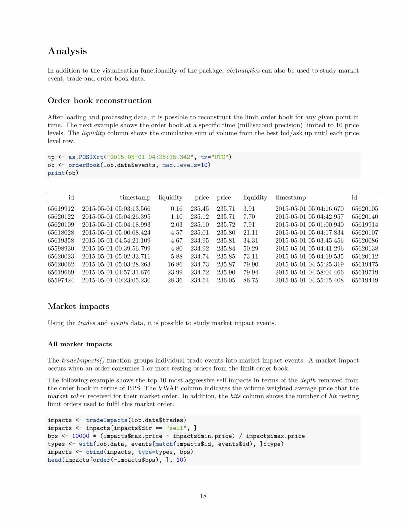
Order book reconstruction

After loading and processing data, it is possible to reconstruct the limit order book for any given point intime. The next example shows the order book at a specific time (millisecond precision) limited to 10 pricelevels. The liquidity column shows the cumulative sum of volume from the best bid/ask up until each pricelevel row.

tp <- as.POSIXct("2015-05-01 04:25:15.342", tz="UTC")ob <- orderBook(lob.data$events, max.levels=10)print(ob)

id timestamp liquidity price price liquidity timestamp id65619912 2015-05-01 05:03:13.566 0.16 235.45 235.71 3.91 2015-05-01 05:04:16.670 6562010565620122 2015-05-01 05:04:26.395 1.10 235.12 235.71 7.70 2015-05-01 05:04:42.957 6562014065620109 2015-05-01 05:04:18.993 2.03 235.10 235.72 7.91 2015-05-01 05:01:00.940 6561991465618028 2015-05-01 05:00:08.424 4.57 235.01 235.80 21.11 2015-05-01 05:04:17.834 6562010765619358 2015-05-01 04:54:21.109 4.67 234.95 235.81 34.31 2015-05-01 05:03:45.456 6562008665598930 2015-05-01 00:39:56.799 4.80 234.92 235.84 50.29 2015-05-01 05:04:41.296 6562013865620023 2015-05-01 05:02:33.711 5.88 234.74 235.85 73.11 2015-05-01 05:04:19.535 6562011265620062 2015-05-01 05:03:28.263 16.86 234.73 235.87 79.90 2015-05-01 04:55:25.319 6561947565619669 2015-05-01 04:57:31.676 23.99 234.72 235.90 79.94 2015-05-01 04:58:04.466 6561971965597424 2015-05-01 00:23:05.230 28.36 234.54 236.05 86.75 2015-05-01 04:55:15.408 65619449

Market impacts

Using the trades and events data, it is possible to study market impact events.

All market impacts

The tradeImpacts() function groups individual trade events into market impact events. A market impactoccurs when an order consumes 1 or more resting orders from the limit order book.

The following example shows the top 10 most aggressive sell impacts in terms of the depth removed fromthe order book in terms of BPS. The VWAP column indicates the volume weighted average price that themarket taker received for their market order. In addition, the hits column shows the number of hit restinglimit orders used to fulfil this market order.

impacts <- tradeImpacts(lob.data$trades)impacts <- impacts[impacts$dir == "sell", ]bps <- 10000 * (impacts$max.price - impacts$min.price) / impacts$max.pricetypes <- with(lob.data, events[match(impacts$id, events$id), ]$type)impacts <- cbind(impacts, type=types, bps)head(impacts[order(-impacts$bps), ], 10)

18

id max.price min.price vwap hits vol end.time type bps65596324 235.09 234.20 234.33 8 37.13 2015-05-01 00:11:01.864 market 37.8665619862 235.77 235.01 235.54 3 0.40 2015-05-01 05:00:08.424 market 32.2365605893 236.96 236.20 236.27 5 8.61 2015-05-01 01:58:18.963 pacman 32.0765619442 235.74 235.06 235.18 13 19.27 2015-05-01 04:55:13.891 market 28.8565596235 235.22 234.55 234.85 2 0.25 2015-05-01 00:10:17.921 pacman 28.4865608339 237.09 236.48 236.61 7 17.25 2015-05-01 02:26:54.539 market 25.7365610618 236.27 235.75 235.77 6 31.21 2015-05-01 02:51:13.180 market-limit 22.0165605081 237.23 236.81 237.06 2 0.05 2015-05-01 01:47:12.365 market 17.7065596651 234.96 234.56 234.74 2 0.25 2015-05-01 00:15:10.098 market 17.0265596775 234.57 234.19 234.35 5 29.53 2015-05-01 00:16:33.253 pacman 16.20

Individual impact

The main purpose of the package is to load limit order, quote and trade data for arbitrary analysis. It ispossible, for example, to examine an individual market impact event. The following code shows the sequenceof events as a single market (sell) order is filled.

The maker.agg column shows how far each limit order was above or below the best bid when it was placed.The age column, shows how long the order was resting in the order book before it was hit by this marketorder.

impact <- with(lob.data, trades[trades$taker == 65596324,c("timestamp", "price", "volume", "maker")])

makers <- with(lob.data, events[match(impact$maker, events$id), ])makers <- makers[makers$action == "created",

c("id", "timestamp", "aggressiveness.bps")]impact <- cbind(impact, maker=makers[match(impact$maker, makers$id),

c("timestamp", "aggressiveness.bps")])age <- impact$timestamp - impact$maker.timestampimpact <- cbind(impact[!is.na(age), c("timestamp", "price", "volume",

"maker.aggressiveness.bps")], age[!is.na(age)])colnames(impact) <- c("timestamp", "price", "volume", "maker.agg", "age")impact$volume <- impact$volume*10^-8print(impact)

timestamp price volume maker.agg age2015-05-01 00:11:01.533 235.09 0.21 16.62 0.891 secs2015-05-01 00:11:01.563 234.70 1.00 5.54 3.331 secs2015-05-01 00:11:01.592 234.70 1.03 0.00 1.094 secs2015-05-01 00:11:01.657 234.42 3.81 -11.93 1.321 secs2015-05-01 00:11:01.720 234.37 9.02 -13.64 6.730 secs2015-05-01 00:11:01.786 234.35 3.68 -14.49 6.128 secs2015-05-01 00:11:01.864 234.20 16.38 -20.88 5.552 secs

19