o3m saf validation report - acsaf.org · function organisation o3m-saf eumetsat, bira-iasb, dlr,...

REFERENCE:

ISSUE:

DATE:

PAGES:

SAF/O3M/IASB/VR/SO2/112

1/1

09 December 2015

of 61

O3M SAF VALIDATION REPORT

Validated products:

Identifier Name Acronym

O3M-54

O3M-55

Near Real Time Total SO2

from GOME-2A&B

MAG-N-SO2

MBG-N-SO2

O3M-09

O3M-56

Offline Total SO2,

from GOME-2A&B

MAG-O-SO2

MBG-O-SO2

O3M-117 Reprocessed Total SO2

from GOME-2A&B MxG-RP1-SO2

REFERENCE:

ISSUE:

DATE:

PAGES:


1/1

09 December 2015

of 61

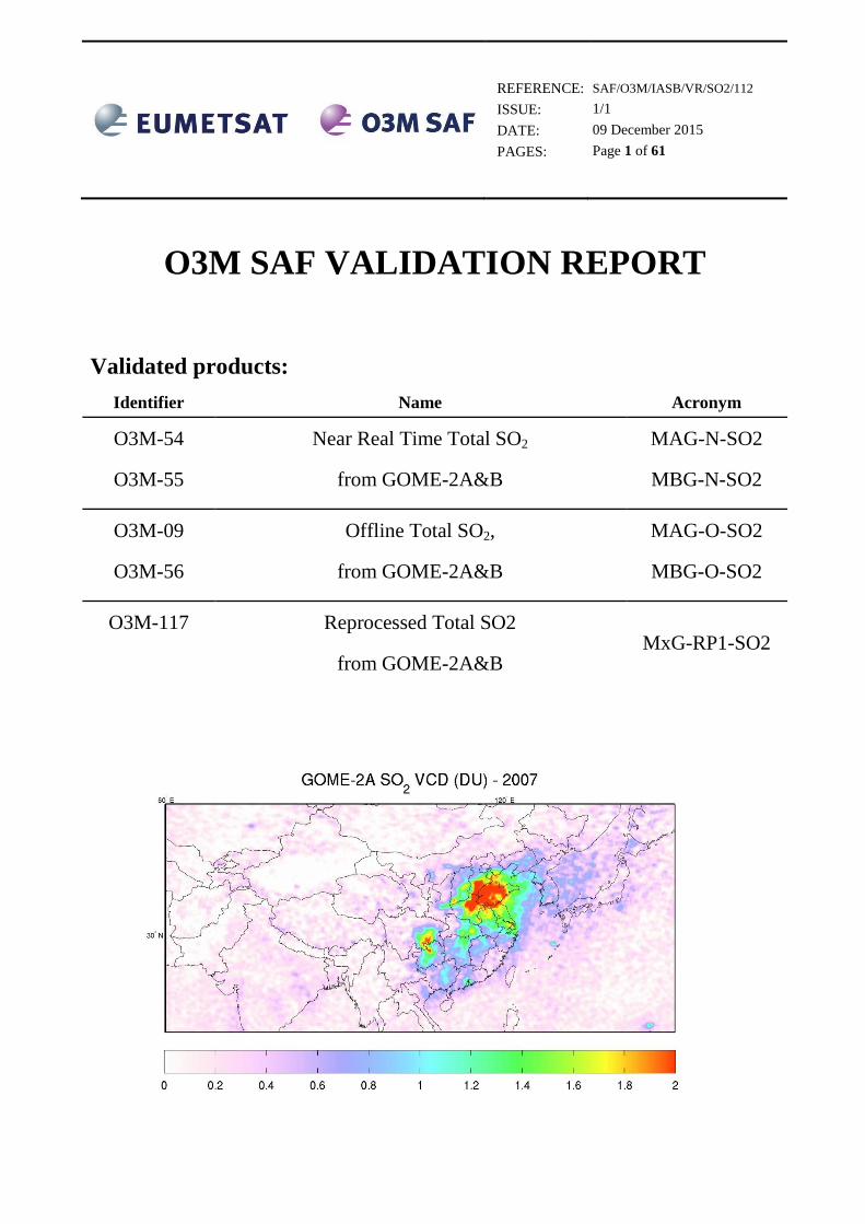
GOME-2A SO2 vertical columns–2007 (China).

Authors:

Name Institute

Nicolas Theys

MariLiza Koukouli

Belgian Institute for Space Aeronomy

Aristotle University of Thessaloniki

Gaia Pinardi Belgian Institute for Space Aeronomy

Michel Van Roozendael

Dimitris Balis

Belgian Institute for Space Aeronomy

Aristotle University of Thessaloniki

Pascal Hedelt German Aerospace Center

Pieter Valks German Aerospace Center

Reporting period: GOME-2/MetOp-A Jan. 2007 – Dec. 2014

GOME-2/MetOp-B Jan. 2013 – Dec. 2014

Input data versions: GOME-2 Level 1B version 5.3.o until 17 June 2014

GOME-2 Level 1b version 6.0.0. since 17 June 2014

Data processor versions: GDP 4.8, UPAS version 1.3.9

revision / revision 1 date of issue / date d’édition December 2015 products / produits MAG-N-SO2, MBG-N-SO2, MAG-O-SO2, MBG-O-SO2, MxG-RP1-SO2 identifier / identificateur O3M-54, O3M-55, O3M-09, O3M-56, O3M-117 product version / version des données level-0-to-1 v5.x and v6.0, level-1-to-2 GDP v4.8

distribution / distribution

Function Organisation O3M-SAF EUMETSAT, BIRA-IASB, DLR, DMI, DWD, FMI, HNMS/AUTH, KNMI, LATMOS, RMI

authors / auteurs N. Theys and M Koukouli

contributeurs / contributors G. Pinardi, M. Van Roozendael, D. Balis, P. Hedelt, and P. Valks

edited by / édité par N. Theys and M. Van Roozendael, BIRA-IASB, Brussels, Belgium

reference / référence SAF/O3M/IASB/VR/SO2/112/TN-IASB-GOME-2-O3MSAF-SO2-2015

document type / type de document O3M-SAF Validation Report issue / edition 1

REFERENCE:

ISSUE:

DATE:

PAGES:


1/1

09 December 2015

of 61

document change record / historique du document

Issue Rev. Date Section Description of Change 1 0 23.09.2015 all Creation of this document

REFERENCE:

ISSUE:

DATE:

PAGES:


1/1

09 December 2015

of 61

Validation report of NRT, offline and

reprocessed GOME-2 SO2 column data for

MetOp-A and -B

Contents

ACRONYMS AND ABBREVIATIONS .............................................................................. 5

DATA DISCLAIMER FOR THE GOME-2 TOTAL SO2 DATA PRODUCTS.............. 7

A. INTRODUCTION ........................................................................................................... 9

A.1 Scope of this document .............................................................................................................. 9

A.2 Preliminary remarks ................................................................................................................... 9

A.3 Plan of this document ................................................................................................................. 9

B. DATA DESCRIPTION ................................................................................................. 10

B.1 SO2 columns retrieval: algorithm description and changes relative to GDP4.7 ....................... 10

B.1.1 Algorithm description .................................................................................................... 10 B.1.2 Changes relative to GDP v4.7 ........................................................................................ 10

B.2 Validation datasets ................................................................................................................... 12

C. EVALUATION OF THE SO2 COLUMN DATA PRODUCT ................................. 13

C.1 Verification of SO2 vertical columns at the global scale .......................................................... 14

C.1.1 Data sets and methodology ............................................................................................ 14 C.1.2 Comparisons between total SO2 columns by the GDP4.7 and GDP4.8 algorithms for GOME-2

MetOp-A and MetOp-B ................................................................................................. 16 C.1.3 Comparisons between total SO2 columns seen by the GOME-2 MetOp-A and -B instruments

and the OMI/Aura datasets ............................................................................................ 30 C.1.4 Conclusions from Section C.1 ....................................................................................... 37

C.2 Verification of SO2 vertical columns for specific volcanic eruptions and anthropogenic SO2 over

China ........................................................................................................................................ 39

C.2.1 Volcanic SO2 .................................................................................................................. 39 C.2.2 Investigating the case for anthropogenic SO2 ................................................................ 43

D. CONCLUSIONS ............................................................................................................ 57

E. REFERENCES .............................................................................................................. 59

E.1 Applicable documents .............................................................................................................. 59

E.2 Reference documents ............................................................................................................... 59

E.2.1 Peer-reviewed articles .................................................................................................... 59 E.2.2 Technical notes .............................................................................................................. 61

REFERENCE:

ISSUE:

DATE:

PAGES:


1/1

09 December 2015

of 61

ACRONYMS AND ABBREVIATIONS

AMF Air Mass Factor, or optical enhancement factor

BAS-NERC British Antarctic Survey – National Environment Research Council

BIRA Belgisch Instituut voor Ruimte-Aëronomie

CAO Central Aerological Observatory

CNRS/LATMOS Laboratoire Atmosphère, Milieux, Observations Spatiales du CNRS

DLR German Aerospace Centre

DMI Danish Meteorological Institute

DOAS Differential Optical Absorption Spectroscopy

D-PAF German Processing and Archiving Facility

Envisat Environmental Satellite

ERS-2 European Remote Sensing Satellite -2

ESA European Space Agency

EUMETSAT European Organisation for the Exploitation of Meteorological Satellites

FMI-ARC Finnish Meteorological Institute – Arctic Research Centre

GAW WMO’s Global Atmospheric Watch programme

GDOAS/SDOAS GOME/SCIAMACHY WinDOAS prototype processor

GDP GOME Data Processor

GOME Global Ozone Monitoring Experiment

GOME-2A Second Global Ozone Monitoring Experiment (MetOp-A)

GOME-2B Second Global Ozone Monitoring Experiment (MetOp-B)

GVC Ghost Vertical Column

H2O water vapour

IASB Institut d’Aéronomie Spatiale de Belgique

IFE/IUP Institut für Fernerkundung/Institut für Umweltphysik

IMF Remote Sensing Technology Institute

INTA Instituto Nacional de Técnica Aeroespacial

KSNU Kyrgyzstan State National University

LOS Line Of Sight

MIPAS Michelson Interferometer for Passive Atmospheric Sounding

NDACC Network for the Detection of Atmospheric Composition Change

NDSC Network for the Detection of Stratospheric Change

NIWA National Institute for Water and Atmospheric research

NO2 nitrogen dioxide

O3 ozone

O3M-SAF Ozone and Atmospheric Chemistry Monitoring Satellite Application Facility

OCRA Optical Cloud Recognition Algorithm

OMI Ozone Monitoring Instrument

ROCINN Retrieval of Cloud Information using Neural Networks

RRS Rotational Raman Scattering

RTS RT Solutions Inc.

SAOZ Système d’Analyse par Observation Zénithale

SCD Slant Column Density

SCIAMACHY Scanning Imaging Absorption spectroMeter for Atmospheric CHartography

SNR Signal to Noise Ratio

SO2 Sulphur dioxide

SZA Solar Zenith Angle

REFERENCE:

ISSUE:

DATE:

PAGES:


1/1

09 December 2015

of 61

TEMIS Tropospheric Emission Monitoring Internet Service

UPAS Universal Processor for UV/VIS Atmospheric Spectrometers

UVVIS ground-based DOAS ultraviolet-visible spectrometer

VCD Vertical Column Density

REFERENCE:

ISSUE:

DATE:

PAGES:


1/1

09 December 2015

of 61

DATA DISCLAIMER FOR THE GOME-2 TOTAL SO2 DATA

PRODUCTS

In the framework of EUMETSAT’s Satellite Application Facility on Ozone and Atmospheric Chemistry

Monitoring (O3M-SAF), GOME-2 SO2 total column data product, as well as associated cloud parameters,

are delivered in near real time and off-line. Those data products are generated at DLR from MetOp-A and

MetOp-B GOME-2 measurements using the UPAS environment version 1.3.9, the level-0-to-1 v5.x and v6.0

processor and the level-1-to-2 GDP v4.8 DOAS retrieval processor. BIRA-IASB, DLR and AUTH ensure

detailed quality assessment of algorithm upgrades and continuous monitoring of GOME-2 SO2 data quality

with a recurring geophysical validation using correlative measurements from ground-based instruments and

from other satellites retrievals.

This report presents the validation of NRT, offline and reprocessed MetOp-A and MetOp-B GOME-2 SO2

column data for the period 2007 to 2014, and retrieved with the GDP4.8 algorithm. The GDP v.4.8

reprocessed dataset was delivered to the validation team in late May 2015. Following the first results of the

validation process which were made available to the operational team, a suite of new GDP4.8 algorithm test

runs were performed for years 2008 and 2013.

The main results are summarized hereafter:

Comparison of GDP4.7 and GDP4.8: For the slant columns, there are negligible differences between

the two versions for GOME-2B while for GOME-2A the slant columns show some differences. An

important feature in GOME-2A is a stronger effect of the South Atlantic Anomaly (see below). For

the vertical columns, the data are found to be noisier in the new version and the GOME-2A GDP4.8

2.5km plume height product shows between 0 and 0.5-1 D.U. higher SO2 loading on a yearly basis

than the GDP4.7 algorithm, whereas for GOME-2B this increase is smaller, between 0 and 0.5 D.U.

at the known hot spots. Retrievals tests have shown that this was due to the use of the inverse of the

Earthshine spectrum in the DOAS intensity offset correction; this issue is largely solved by using

instead the inverse of the Solar spectrum. This setting is the new baseline for the GDP4.8 SO2

algorithm.

GOME-2A- GOME-2B-OMI consistency: 33 known SO2 emitting locations around the world,

including volcanoes, power plants, smelters, and so on, were used to compare the GOME-2A and -

2B SO2 to the OMI estimates. The average SO2 loading of these sources was 0.41±0.31 D.U. for

GOME-2A, 0.08±0.24 D.U. for GOME-2B and 0.30±0.31 D.U. for OMI. GOME-2A was found to

be in better agreement with OMI than GOME-2B GDP4.8 due to the higher amount of negative

mean loadings shown by the newer instrument. However, the mean correlation coefficient for these

sites between GOME2 and OMI was found to be 0.42 for GOME-2A and 0.51 for GOME-2B

pointing to the fact that both GOME-2A and –2B GDP 4.8 SO2 column retrievals fare well with

OMI/Aura considering all the limitations.

Volcanic SO2: GOME-2A and –B GDP 4.8 SO2 column retrievals is clearly able to capture and track

plumes after small to strong eruptions, but the newly implemented flag for volcanic SO2 misses parts

of aged and filamentary plumes. Quantitatively, the SO2 masses estimated from GOME-2 after

strong eruptions agree very well with OMI (with differences mostly within the 30% optimal

accuracy), except for the rather unusual very high SO2 amounts (for the first days after the start of the

eruption) where GOME-2 underestimates the columns (saturation effect).

Anthropogenic SO2: the addition of a new SO2 column in GDP4.8 using a typical profile for

anthropogenic emissions scenario is an improvement and allows direct comparison with OMI. From

REFERENCE:

ISSUE:

DATE:

PAGES:


1/1

09 December 2015

of 61

comparisons with OMI, it can be concluded that 1) several hotspots are seen by both satellite

datasets and the mean values from GOME-2 and OMI are reasonably close, 2) some weak emissions

are not detected by GOME-2, partly because of the better spatial resolution of OMI but also because

GOME-2 data is more noisy. From the comparison (using the anthropogenic SO2 column field) with

the MAXDOAS-data, the best agreement is found for the results using clear-sky AMFs (while the

results for total AMFs are always found lower). The agreement is reasonably good especially for

non-winter periods and the product reaches often the target/optimal accuracy (50%/30%) and the

threshold accuracy (100%) otherwise.

Localized artifacts and product self-inconsistency: Several artifacts have been identified when

viewing SO2 maps as, for e.g., at high latitudes. Over the SAA region specifically, the GOME-2 data

shows a dramatic trend over time with noisy and elevated SO2 columns over the last years (this

effect is worst in GDP4.8 than in GDP4.7). This feature is due to the treatment of the DOAS

intensity offset correction. An investigation of the SO2 SCDs over clean and polluted regions shows

an anomalous dependence of the results with viewing angles for both sensors. The most likely

explanation for this effect is due to differences between the slit functions used in the spectral fitting

(extracted from the GOME-2 key data) and the actual ones.

REFERENCE:

ISSUE:

DATE:

PAGES:


1/1

09 December 2015

of 61

A. INTRODUCTION

A.1 Scope of this document

The present document reports on the validation of NRT, offline and reprocessed GOME-2/MetOp-A and

MetOp-B SO2 column data acquired since the beginning of instrument operations. The data are produced

operationally by the GOME Data Processor (GDP) operated at DLR in the framework of the EUMETSAT

Satellite Application Facility on Ozone and Atmospheric Chemistry Monitoring (O3M-SAF). This report

addresses the quality of individual components of the data processing, starting with DOAS fitting

parameters. The report includes comparisons of GOME-2 final data products with correlative observations

from independent sources, namely, total SO2 column data produced with GDP versions 4.7, OMI and MAX-

DOAS observations.

A.2 Preliminary remarks

The aim of the present document is to report on the validation of the GOME-2 SO2 columns from MetOp-A

and MetOp-B (hereafter referred as GOME-2A and GOME-2B, respectively) against various satellite data

sets and ground-based data.

Reported validation studies were carried out at the Belgian Institute for Space Aeronomy (IASB-BIRA,

Brussels, Belgium), at the Aristotle University of Thessaloniki (AUTH) and at DLR Remote Sensing

Technology Institute (DLR-IMF, Oberpfaffenhofen, Germany) in the framework of EUMETSAT Satellite

Application Facility on Ozone and Atmospheric Chemistry Monitoring (O3M-SAF).

A.3 Plan of this document

This document is divided in three main parts, addressing first of all the account of the retrieval settings

applied for the SO2 product including a detailed description of the changes brought by GDP4.8 compared to

GDP4.7. Then, the GDP4.8 GOME-2A and GOME-2B Slant and Vertical column products are evaluated

against the equivalent GDP4.7 products as well as OMI/Aura measurements. The anthropogenic SO2

products are studied using known hot-spots on a global scale and are also validated against a MaxDOAS

ground-based instrument located in China. The volcanic SO2 product is also examined in detail through inter-

comparisons of the different algorithm settings as well as towards OMI/Aura findings. The stability of the

GOME-2A and GOME–2B SO2 column products as a function of time is also inspected in detail.

REFERENCE:

ISSUE:

DATE:

PAGES:


1/1

09 December 2015

of 61

B. DATA DESCRIPTION

B.1 SO2 columns retrieval: algorithm description and changes relative to

GDP4.7

B.1.1 Algorithm description

The operational retrieval of total SO2 columns from the GOME-2 instrument aboard MetOp-A and –B

involves a two-step procedure:

First, a DOAS retrieval is performed in the wavelength region 315-326nm, in which cross-sections of SO2,

O3 and NO2 are fitted to the UV Earth reflectance spectrum. The retrieved SO2 slant column is then corrected

for any instrumental bias by applying a latitude and surface-altitude dependent offset correction. The

correction factors are determined in 14-days moving time window. The corrected slant columns are then

corrected for the atmospheric temperature in which the SO2 concentration is expected. This is a priori not

known, hence the user is provided with a set of SO2 results for a set of three pre-defined volcanic and one

anthropogenic scenario.

Secondly, the background and temperature corrected slant columns are converted to total vertical columns by

means of an Air Mass Factor (AMF). Again, for every scenario a single-wavelength AMF (at 320nm) is

applied. This AMF is based on a priori profile shapes for volcanic eruption scenarios (i.e. Gaussian shaped at

prescribed plume heights) and for the anthropogenic SO2 column product based on aircraft measurements

from Taubmann et al. (2006).

B.1.2 Changes relative to GDP v4.7

In a previous validation report (Theys et al., 2013), SO2 columns retrieved from GOME-2/MetOp-A &-B

using the operational GDP4.6 processor were evaluated for the years 2007 to 2013. Since 2013 GOME-

2/MetOp-B data is provided on an operational basis.

In order to provide an improved dataset and to fulfill user demands, an updated operational processor version

4.8 was developed. This updated version incorporates the following points:

Harmonization of retrieval settings between both GOME-2 sensors

In GDP4.7 a different treatment of instrumental straylight was used for both instruments: For

GOME-2A an inversed solar irradiance spectrum was fitted in the DOAS retrieval, whereas for

GOME-2B an inversed Earthshine spectrum was used. The usage of an inversed Earthshine

spectrum follows directly from the linearization of Beer’s Law when an offset term is added. Also

the polynomial degree to correct for broadband absorption features was different (3rd

order for

GOME-2A and 5th order for GOME-2B). In order to use harmonized settings for both sensors it was

decided to use an inversed Earthshine spectrum for the straylight correction and a 5th order

polynomial for the GDP4.8 dataset that is validated in this report. Note that at a later stage after a

first draft version of this verification report, it was found that using an inversed Earthshine spectrum

results in an increased noise level and long-term trends. The final GDP4.8 dataset to be released will

thus incorporate an inversed solar irradiance spectrum for both instead.

Improved retrieval settings

The SO2 cross-section used for the retrieval are based on SCIAMACHY flight model measurements.

In order to apply them to GOME-2 data it is required to deconvolve the cross-section with

REFERENCE:

ISSUE:

DATE:

PAGES:


1/1

09 December 2015

of 61

SCIAMACHY slit function data and convolve it with the appropriate GOME-2 slit function. An

updated deconvolution process was implemented for GDP v4.8 improving the quality of the SO2

cross-section data and thus the SO2 retrieval

New anthropogenic SO2 scenario

In GDP4.7 only a set of three total SO2 vertical columns have been provided for three volcanic

eruption scenarios (i.e. SO2 plumes at 2.5, 6, and 15km). It is however of increasing interest of the

user community to also have SO2 retrievals for anthropogenic pollution scenarios, for which the 2.5

km plume height scenario is clearly not appropriate. Thus, for GDP 4.8 an anthropogenic SO2 profile

is used for the generation of AMFs. This profile is based on aircraft measurements (Taubmann et al.

2006)

Flagging of volcanic SO2 plumes

A new volcanic activity detection algorithm has been implemented in the operational GDP v4.8

retrieval. This algorithm is based on algorithm used by the SACS project (Support to Aviation

Control Service) and described in Brenot et al. (2014). The original SACS algorithm was adjusted to

identify the entire volcanic SO2 plume using different threshold values for the vertical SO2 column

depending on the proximity to known volcanoes or polluted areas (anthropogenic or the SAA). In

the final product a new flag was added that provides the user with the information whether a pixel

shows increased SO2 values due to volcanic activity. In order to reduce false-positive detections over

polluted areas the flag can take different values. However it should be noted that the detection

algorithm is very conservative and so far no false-positive detection have been found, even in

polluted areas.

Cloud algorithm changes

Within GDP4.7, geometric cloud fractions determined by OCRA/ROCINN were employed. It is

however found that it is better to use Intensity weighted Cloud Fractions (IWCF) that take into

account the wavelength dependency of the cloud fraction. There is no dedicated algorithm to

calculate this for the SO2 fit window (315-326nm) and hence, in GDP4.8, the IWCF explicitly

calculated from the O3 fit window (325-335nm) is used. This wavelength window is of course not

the same as for the 315-326nm window but is a much better estimate as using the geometric cloud

fraction enforced so far.

Table I. DOAS settings used for the GOME-2 SO2 retrieval GDP4.8.

Fitting interval 315 – 326 nm

Sun reference Sun irradiance for GOME-2 L1 product

Wavelength calibration Wavelength calibration of sun reference optimized by NLLS adjustment on

convolved Chance and Spurr solar lines atlas

Absorption cross-sections

- SO2 Updated reconvolved SCIA Flight Model [Bogumil et al., 2003], 203K (15

km)

- NO2 GOME-2 Flight Model/CATGAS [Gür et al., 2005], 241 K

- O3 Brion et al. [1998], 218 K and 243 K, reconvolved at GOME-2 resolution

Two pseudo-cross-sections accounting for interference between SO2 and O3

- Ring effect 2 Ring eigenvectors generated using SCIATRAN

REFERENCE:

ISSUE:

DATE:

PAGES:


1/1

09 December 2015

of 61

- Instrumental

straylight

Inversed earthshine spectrum from L1 data (original verification dataset)

Inversed solar spectrum from L1 data (revised final verification dataset)

Polynomial 5th order (6 parameters)

SCD background

correction

Latitude and surface-altitude dependent offset, determined from a 14day

moving average

B.2 Validation datasets

The SO2 columns in the atmosphere may vary greatly from about 1DU level for anthropogenic SO2 and low

level volcanic degassing to 10-1000DU for medium to extreme volcanic explosive eruptions. This wide

range of possible values/scenarios makes any attempt to validate the GOME-2 total SO2 column product a

difficult task:

Anthropogenic/boundary layer SO2: the measurement of SO2 is a challenge because of the low

column amount (especially for GOME-2 at moderate spatial resolution) and reduced measurement

sensitivity close to the surface and the SO2 signal is generally overwhelmed by the competing O3

absorption. The column accuracy is directly affected by the quality of the background correction

applied. In this work, we will use SO2 column (and profile) retrievals from a ground-based MAX-

DOAS instrument at Xianghe, China (Wang et al., 2014) to validate the GOME-2 SO2 products. No

attempts will be made to use the Brewer Network as the data quality is deemed insufficient for

validation of anthropogenic SO2.

Volcanic SO2: the measurement is facilitated by large SO2 columns generally at high altitudes (free-

troposphere to lower stratosphere). However, for large SO2 columns (typically >50 DU) the SO2

absorption tends to saturate leading to a general underestimation of the SO2 columns, affecting

directly the product accuracy. For most volcanoes, there is generally no ground-based equipment to

measure SO2 during an appreciable eruption and even if it is the case, the data are generally very

difficult to use for validation. In practice, dedicated aircraft campaign flights can also measure

volcanic SO2 clouds, but rely on the occurrence of volcanic events and there is only a handful of

datasets available. In the present study, the approach that has been adopted is to verify/validate the

GOME-2 SO2 column product through cross-comparisons with SO2 column products from OMI.

Before showing any results, it is good to recall the user requirements for the GOME-2 SO2 products in terms

of accuracy as these numbers will guide us in the present report: Threshold accuracy: 100%; Target

accuracy: 50% (for solar zenith angles lower than 70°); Optimal accuracy: 30%. These numbers are taken

from the O3MSAF Service Specification Document, available at

http://o3msaf.fmi.fi/docs/O3M_SAF_Service_Specification.pdf.

http://o3msaf.fmi.fi/docs/O3M_SAF_Service_Specification.pdf

REFERENCE:

ISSUE:

DATE:

PAGES:


1/1

09 December 2015

of 61

C. EVALUATION OF THE SO2 COLUMN DATA PRODUCT

Before showing results, it is important to remind the evolution of the data quality as a function of time.

Figure 1 illustrates the fitting residuals and slant column errors (averaged over the equatorial pacific) as a

function of time, both for GOME-2 onboard MetOp-A and MetOp-B (hereafter referred as GOME-2A and

GOME-2B, respectively). From Figure 1, one can see the GOME-2A suffers for many years of a strong

instrumental degradation affecting the quality of the SO2 column product (e.g., the data scatter has more than

doubled since the beginning of operations) but after the 2009 throughput test the residual are reasonably

stable over time. The GOME-2B data starting from Dec. 2012 seems to be of similar quality than GOME-2A

in early 2007 (beginning of operations) but one can also see a quite strong increase of the residuals and data

scatter as a function of time.

Figure 1. Average DOAS fitting residuals (upper panel) and slant column error (lower panel) in the

equatorial Pacific (Lat: 20N-20S, Lon: 160W-160E) as a function of time for GOME-2A (black) and

GOME-2B (red).

In the following, we will first evaluate the SO2 at the global scale (section D1) by comparing GDP4.7 and

GDP 4.8 but also assess the consistency of GDP4.8 GOME-2A, GOME-2B and OMI results. In section D2,

we will focus more in details on several comparison cases for volcanic and anthropogenic SO2 scenarios.

REFERENCE:

ISSUE:

DATE:

PAGES:


1/1

09 December 2015

of 61

C.1 Verification of SO2 vertical columns at the global scale

C.1.1 Data sets and methodology

The GOME2/MetopA and GOME2/MetopB GDP4.7 total SO2 column measurements contain three different

column products: one assuming the SO2 load is located near the planetary boundary layer at 2.5km altitude,

one assuming the SO2 is located in the free troposphere at 6km altitude and one assuming the SO2 has

volcanic eruptive provenance and has crossed the tropopause and is located at 15km altitude. For the

following comparisons, the lowermost column [reported at 2.5km] will be utilized.

The GOME2/MetopA and GOME2/MetopB GDP4.8 total SO2 column measurements contain, additionally

to the columns described above, a column at 1km, of pure anthropogenic provenance. For the GDP4.8

datasets hence both the data associated with this column, as well as the traditional 2.5km column as well as

this new column, will be examined in the following.

The GOME2/MetopA and GOME2/MetopB GDP4.7 & GDP4.8 SO2 columns have been filtered using the

following choices: data are accepted for the analysis if the associated intensity weighted cloud fraction is less

than 20%, the solar zenith angle less than 60° and the quality flag as well as the SO2 associated quality flag

equal zero [denoting completely trouble-free data points]. Furthermore, only forward pixels from the

descending node observations were allowed for these comparisons. The updated cloud algorithm retrieval

associated with GDP4.8 is also expected to result in altered VCDs, due to the new associated AMF

calculations.

The OMI/Aura NASA Sulphur Dioxide Level 2G Global Binned (0.125 deg Lat/Lon grids) Data Product-

OMSO2G was downloaded from the GODDARD Earth Sciences Data and Information Services Center1.

The Planetary Boundary Layer (PBL) SO2 column (ColumnAmountSO2_PBL), corresponding to a Centre of

Mass Altitude, CMA, of 0.9 km, was examined with the same restrictions applied above. The OMI columns

will be used as a backdrop onto which the differences between GDP4.7 and GPD4.8 can be assessed and

possible differences between GOME-2A and GOME-2B rooted out.

All datasets were then averaged onto a 1x1° grid on a global scale and monthly basis and the mean SO2 load,

associated standard deviation of the mean, average reported error value as well as the standard deviation of

the error value was saved in a monthly mean data file. This gridding was also performed using an area

average technique whereupon each monthly 1x1° grid was not only allocated the measurements it

represented by also a weight of the eight surrounding cells, hence introducing a spatial “smoothing” which

cleared-up some of the noise associated with these measurements. From the monthly mean data, seasonal and

yearly mean products were created for viewing and comparison purposes. Hence, two products will be

shown in the following, the simple mean and the area weighted mean.

In order to perform quantitative comparisons between the datasets, apart from the monthly, seasonal and

yearly products, a sample of selected locations on a global scale was chosen for detailed study and shown in

Table II. Those sites represent well-known and well-documented, as well as important, SO2 sources of both

natural and anthropogenic origin. For these locations, the datasets were averaged on a finer grid of 0.25x025°

grid in that case around 2.5° from the location center. Scatter plots and statistics are hence presented for

those sites in order to assure a high enough SO2 signal from the satellite observations.

1 http://disc.sci.gsfc.nasa.gov/Aura/data-holdings/OMI/omso2g_v003.shtml

http://disc.sci.gsfc.nasa.gov/Aura/data-holdings/OMI/omso2g_v003.shtml

REFERENCE:

ISSUE:

DATE:

PAGES:


1/1

09 December 2015

of 61

Year 2008 was chosen as representative of the beginning of the GOME2/MetopA mission and year 2013 for

GOME2/MetopB.

Table II. List of locations studied as major SO2 sources on a global scale.

LATITUDE LONGITUDE TYPE NAME LOCATION

1 -37.85 -71.16 Volcano Copahue Copahue

2 -26.57 29.17 Power_Plants South_Africa South_Africa

3 -17.63 -71.34 Smelter and Volcano Ilo, Ubinas Peru

4 -16.25 168.12 Volcano Ambrym Vanuatu

5 -8.27 123.51 Volcano Lewotolo Indonesia

6 -7.94 112.95 Volcano East Java Indonesia

7 -6.09 155.23 Volcano Bagana Papua New Guinea

8 -4.12 152.2 Volcano Turvurvur/Rabaul Papua New Guinea

9 -4.08 145.04 Volcano Manam Papua New Guinea

10 -1.41 29.2 Volcano Nyiragongo

Democratic Republic of

Congo

11 1.68 127.88 Volcano Dukono Indonesia

12 13.26 123.69 Volcano Mayon Philippines

13 16.35 145.67 Volcano Anatahan Northern Mariana Islands

14 16.72 -62.18 Volcano Soufrière Hills Montserrat (UK)

15 19.08 -104.28 Power Plant Manzanillo Mexico

16 19.4 -92.24 Oil industry

Oil fields in Gulf of

Mexico Mexico

17 19.48 -155.61 Volcano Kilauea, Hawaii U.S.

18 20.05 -99.28

Industrial and

Volcano Tula, Popocatepetl Mexico

19 20.63 39.56 Oil industry Shoaiba Saudi Arabia

20 23.12 113.25 Multiple sources Guangdong China

21 29.22 50.32 Oil industry Khark Island Iran

22 29.98 55.86 Smelter Sarcheshmeh Iran

23 34.08 139.53 Volcano Miyake-jima Japan

24 37.12 22.11 Power_Plants Balkans Balkans

REFERENCE:

ISSUE:

DATE:

PAGES:


1/1

09 December 2015

of 61

25 37.73 15 Volcano Mt. Etna Italy

26 39.44 106.72 Multiple sources Shizuishan China

27 39.9 116.38 Multiple sources Eastern_China Eastern_China

28 42.15 25.91 Power Plants Marica Bulgaria

29 44.67 23.41 Power Plants Rovinary, Turceni, Isalnita Romania

30 46.83 74.94 Smelter Balqash Kazakhstan

31 69.36 88.13 Smelter Norilsk Russia

C.1.2 Comparisons between total SO2 columns by the GDP4.7 and GDP4.8 algorithms for

GOME-2 MetOp-A and MetOp-B

In Figure 2 the global SO2 load at 2.5km seen by GOME-2A is given for the current GDP4.7 (left) and the

new GDP4.8 (right) algorithms. Year 2008 was chosen as it was the beginning for the GOME-2A mission

and hence the least possible instrumental degradation is present to affect our comparisons. Even though the

general features appear similar, a number of issues may already be identified such as the South Atlantic

Anomaly (SSA) producing high SO2 values in the new version of the data. Some of the higher values in the

high latitudes of the Northern Hemisphere, especially in North America/Canada but also in Siberia, are

attributable to the Kasatochi Volcano, an active stratovolcano, in the Aleutian Islands of Southwestern

Alaska.

Figure 2: The global SO2 load at 2.5km as seen by GOME-2A GDP4.7 (left) and GDP 4.8 (right) is shown

for year 2008.

In Figure 3 the global mean SO2 load at 2.5km seen by GOME-2B is given for the current GDP4.7 (left) and

the new GDP4.8 (right) algorithms for year 2013, the beginning of the MetopB mission. It is obvious that the

data is far less noisy, with the abnormally high values in the Northern high latitudes disappearing and known

hot spots appearing clearly such as the Nyiragongo and Nyiamuragira Volcanoes, in the Democratic

Republic of Congo, in Africa, volcanic activity from Popocatepetl as well as industrial activity in Mexico, in

addition to the industrial regions south of Beijing in China. Some issues remain for the SAA region while it

REFERENCE:

ISSUE:

DATE:

PAGES:


1/1

09 December 2015

of 61

appears as though the GOME-2B GDP4.8 algorithm is producing lower SO2 loading than the GDP4.7

algorithm, to be discussed further below.

Figure 3. The global SO2 load at 2.5km as seen by GOME-2B GDP4.7 (left) and GDP 4.8 (right) is shown

for year 2013.

Figure 4. The global SO2 load at 1km (left) and 2.5km (right) as seen by GOME-2A GDP4.8 is shown for

year 2008.

In Figure 4 a first visual comparison is shown for the new 1km anthropogenic product (left) provided by the

GDP4.8 algorithm against the traditional 2.5km product (right) for year 2008. Undoubtedly, the 1km product

is, as expected from the lower AMFs, noisier on a global scale and seems to provide higher SO2 values at the

known hot-spots, with the Kīlauea eruptions in Hawaii appearing stronger, as well as the hotspots in China.

As discussed above, the similar picture for GOME-2B GDP4.8 (Figure 5) is less noisy, even though the SSA

area is still noisier due to the lower AMFs calculated and the signal retrieved for the 1km product is indeed

higher.

REFERENCE:

ISSUE:

DATE:

PAGES:


1/1

09 December 2015

of 61

Figure 5. The global SO2 load at 1km (left) and 2.5km (right) as seen by GOME-2B GDP4.8 is shown for

year 2013.

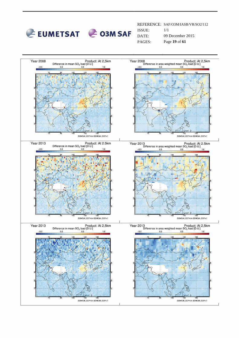
A simple example of the actual differences between the new algorithm and the current one is given in Figure

6 for China. In the first row, the differences between GOME-2A GDP4.8 and GDP4.7 for year 2008, in the

middle row, the differences between GOME-2A GDP4.8 and GDP4.7 for year 2013 and in the bottom row,

the differences between GOME-2B GDP4.8 and GDP4.7 for year 2013.

The absolute differences are shown since most pixels in this domain are related to near-zero values which

made a very noisy percentage difference plot. In the left column, the differences of the row plots shown in

Figure 6 reveal the higher SO2 value reported by GOME-2A GPD4.8 for the hotspot region in China of

almost 50% for the entire polluted region and of close to 10-20% and only for some central spots for GOME-

2B. For GOME-2A for the year 2008 [top row] no variations are seen in the absolute differences of the

hotspots. Year 2013 [middle and bottom rows] is obviously noisier due to the instrumental degradation

effects. However, the actual differences in the SO2 sources remain of the same order of magnitude

irrespective of the year shown.

In the right column of Figure 6 we give the differences for the area weighted mean SO2 load. Even though

for such a coarse grid of 1x1° this dataset can only be used for pictorial reasons, the high latitude issues

identified in previous Figures are revealed here, Northwards of 55°N, where the SO2 field is no longer

smooth but strong pixelation appears.

The Himalayan plateau appears white [i.e. no data] since no GDP4.8 retrievals passed the restriction

selection enumerated in Section C.1.1.

REFERENCE:

ISSUE:

DATE:

PAGES:


1/1

09 December 2015

of 61

REFERENCE:

ISSUE:

DATE:

PAGES:


1/1

09 December 2015

of 61

Figure 6. Left column. Absolute differences between GOME-2A GDP4.8 and GDP4.7 for 2008 [top]; same

for 2013 [middle] and between GOME-2B GDP4.8 and GDP4.7 for 2013 [bottom]. Right column. Same as

the left column, but for the area weighted mean SO2 load.

In the next section the aim is to show that the two instruments see the same atmospheric state, analyzed with

either the new GDP4.8 algorithm or with the original GDP4.7 one. Year 2013 will be used as a reference

point. The new algorithm is expected to homogenize the SO2 loadings seen by the two instruments and to

have improved issues already identified in the previous validation effort such as the general tendency of

GOME-2B to produce lower columns than GOME-2A by about 5-10% depending on the region examined.

From Figure 7, where the comparison is shown for the Asia region for year 2013 for both algorithms and

instruments we can already see the differences between the two instruments already identified in the previous

validation effort (top row). These differences do not appear to be smoothed out with the new algorithm

(bottom row). GOME2-A for year 2013 is generally noisier. For GOME-2B, it can be seen that the higher

values over the Eastern China are a bit lower in GDP4.8 and 4.7 (possibly because of the different cloud

algorithm leading to a slightly different cloud masking). The noise on the GOME2 (A and B) VCDs seems to

be higher as well for the new algorithm.

REFERENCE:

ISSUE:

DATE:

PAGES:


1/1

09 December 2015

of 61

Figure 7: Comparison between GOME-2A and GOME-2B GDP4.7 (upper) and GDP4.8 (lower) for year

2013 zooming into Asia. GOME-2A is on the left and GOME-2B on the right column.

Figure 8. Time-series of weekly averaged SO2 background corrected slant columns over Mauna Loa

(19.53°N,155.58°W), Linan (30.3°N, 119.73°E) and Xianghe (39.98°N, 116.37°E) for GOME-2A (left plots)

and GOME-2B (right plots) comparing GDP versions 4.7 (black line) and 4.8 (red line) for the period July

2013-December 2014. The blue curves show the differences between the SO2 SCDs of versions 4.8 relative

to 4.7. The pixels in a circle of 150 km radius around the stations are considered for SZA less than 70°.

REFERENCE:

ISSUE:

DATE:

PAGES:


1/1

09 December 2015

of 61

Figure 8 shows examples of comparisons between SO2 SCDs (GDP4.7 vs GDP4.8) for selected locations

(Mauna Loa in Hawai in the top row, Linan and Xianghe in China in the middle and bottom rows) both for

GOME-2A and –B. Generally, the GOME-2B results for the different versions are very close and the

differences are always lower than 0.1 DU. This means that the differences seen in the VCDs in Figure 7 are

coming from the AMFs (most likely from the update in the cloud products).

In contrast, the differences between GOME-2A GDP4.8 and 4.7 SO2 SCDs are much larger than in the case

of GOME-2B and the reason for the discrepancy for GOME-2A only is due to the fact that the upgrade from

GDP4.7 to GDP4.8 for that instrument necessitated a lot more changes as seen in Section B.1.2.

In order to understand the differences between GDP4.7 and GDP4.8 SO2 products better, several iterative

discussions with the operational algorithm team at DLR have taken place. Note that most of this report is

based on the original GDP v4.8 dataset delivered to the validation teams in late May 2015. Some of the

problems of the new dataset identified in this report have already been taken into account in a suite of new

GDP4.8 algorithm test runs performed by the operational team for years 2008 and 2013.

For GDP v.4.8 the initial idea was to harmonize the retrieval settings between GOME-2A and GOME-2B

and thus using an Inversed Earthshine spectrum was selected. One important issue identified in this report is

a generally higher noise level in the GDP v4.8 data, which is especially visible in the SAA region. This

effect is mainly visible for the GOME-2A data and, to a lesser extent, for GOME-2B data. The reason for

this was a different treatment of intensity offset correction in the DOAS retrievals for GOME-2A and

GOME-2B in GDP v4.7: In GDP v4.7, for GOME-2A data an Inversed solar irradiance spectrum was fitted,

whereas for GOME-2B an Inversed Earthshine spectrum was used.

After this problem was identified by the validation team, a drift analysis however revealed that using an

Inversed Earthshine spectrum leads not only to much higher noise levels in the SO2 retrieval but also causes

a trend in the SO2 dataset over regions with no known and major SO2 sources (see red line in Figure 9). This

is probably related to the degradation of the instrument which affects the Earthshine data used for the offset

correction.

This higher noise level is unfortunately not visible in the daily data or on short timeframes. This is the reason

why it was not identified as a problem for the GOME-2B GDP v4.7 retrieval in the last validation report.

In the new GDP v4.8 retrieval settings [see blue lines in Figure 9] both instruments now use an Inversed

solar irradiance spectrum. With this, the noise levels are much reduced, especially in the SAA region. Also

no drifts are visible in SO2-free regions.

REFERENCE:

ISSUE:

DATE:

PAGES:


1/1

09 December 2015

of 61

Figure 9: Monthly averaged SO2 time series for GOME-2A (top) and GOME-2B (bottom) for the SAA

region between -60°S and -10°S and -100°W and 0. Clearly visible is an increasing SO2 trend for the GDP

v.4.8 dataset used in this validation report (red). After identification of the problem, a corrected dataset has

been generated for some selected years (blue).

REFERENCE:

ISSUE:

DATE:

PAGES:


1/1

09 December 2015

of 61

REFERENCE:

ISSUE:

DATE:

PAGES:


1/1

09 December 2015

of 61

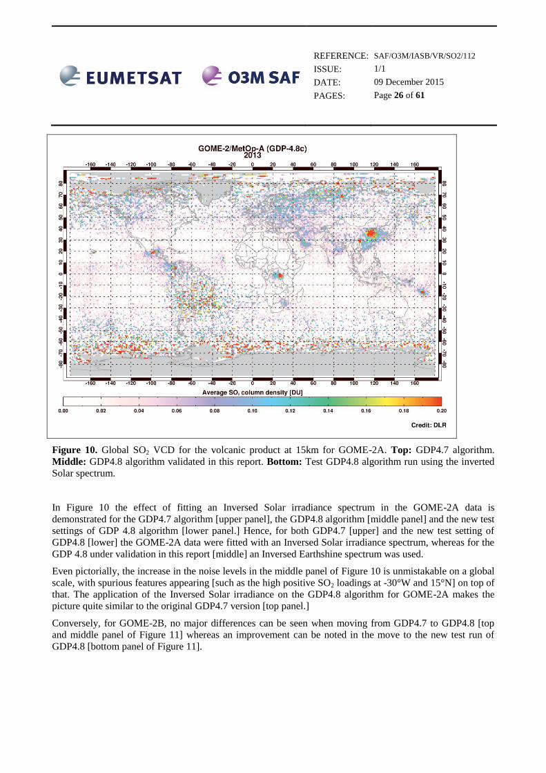
Figure 10. Global SO2 VCD for the volcanic product at 15km for GOME-2A. Top: GDP4.7 algorithm.

Middle: GDP4.8 algorithm validated in this report. Bottom: Test GDP4.8 algorithm run using the inverted

Solar spectrum.

In Figure 10 the effect of fitting an Inversed Solar irradiance spectrum in the GOME-2A data is

demonstrated for the GDP4.7 algorithm [upper panel], the GDP4.8 algorithm [middle panel] and the new test

settings of GDP 4.8 algorithm [lower panel.] Hence, for both GDP4.7 [upper] and the new test setting of

GDP4.8 [lower] the GOME-2A data were fitted with an Inversed Solar irradiance spectrum, whereas for the

GDP 4.8 under validation in this report [middle] an Inversed Earthshine spectrum was used.

Even pictorially, the increase in the noise levels in the middle panel of Figure 10 is unmistakable on a global

scale, with spurious features appearing [such as the high positive SO2 loadings at -30°W and 15°N] on top of

that. The application of the Inversed Solar irradiance on the GDP4.8 algorithm for GOME-2A makes the

picture quite similar to the original GDP4.7 version [top panel.]

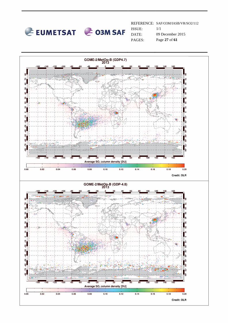
Conversely, for GOME-2B, no major differences can be seen when moving from GDP4.7 to GDP4.8 [top

and middle panel of Figure 11] whereas an improvement can be noted in the move to the new test run of

GDP4.8 [bottom panel of Figure 11].

REFERENCE:

ISSUE:

DATE:

PAGES:


1/1

09 December 2015

of 61

REFERENCE:

ISSUE:

DATE:

PAGES:


1/1

09 December 2015

of 61

Figure 11. Global SO2 VCD for the volcanic product at 15km for GOME-2A. Top: GDP4.7 algorithm.

Middle: GDP4.8 algorithm validated in this report. Bottom: Test GDP4.8 algorithm run using the inverted

Solar spectrum.

Quite similarly, as was shown in Figures Figure 10 and Figure 11 for the volcanic product, we show in

Figure 12 the anthropogenic product at 2.5km for GOME-2A [upper] and GOME-2B [lower] for the new test

settings of GDP4.8. The differences between the two instruments are quite distinct, with GOME-2A

suffering not only from the higher noise levels, which sometimes reach the levels of known hot-spots, but

also in the location and extend of said known hot-spot regions.

REFERENCE:

ISSUE:

DATE:

PAGES:


1/1

09 December 2015

of 61

REFERENCE:

ISSUE:

DATE:

PAGES:


1/1

09 December 2015

of 61

Figure 12. Global SO2 VCD for the anthropogenic product at 2.5km for GOME-2A [upper] and GOME-2B

[lower] for the test GDP4.8 algorithm run using the inverted Solar spectrum.

C.1.3 Comparisons between total SO2 columns seen by the GOME-2 MetOp-A and -B

instruments and the OMI/Aura datasets

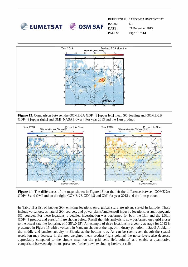
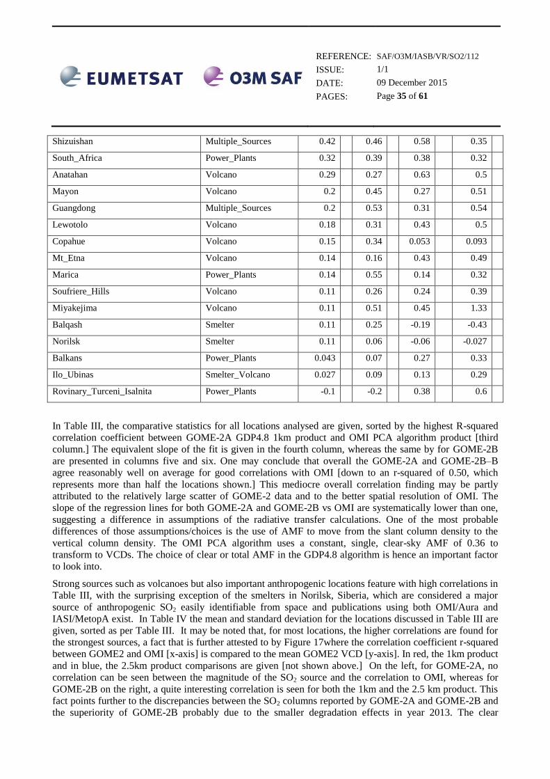
In Figure 13, the GDP4.8 1km product is now compared to the OMI NASA SO2 load. GOME-2A is shown

on the upper left and GOME-2B on the upper right and the OMI product at the bottom. The two instruments

do differ in GDP4.8 both in the background values and the hotspot magnitude, albeit with smaller differences

that in GDP4.7. In Figure 14 the differences between GOME-2A and GOME-2B against the OMI data are

shown. The GOME-2B differences (right) are larger in magnitude and affect both the background and the

hotspots, showing a GOME-2B under-estimation against OMI which is not repeated in the GOME-2A maps

(left).

REFERENCE:

ISSUE:

DATE:

PAGES:


1/1

09 December 2015

of 61

Figure 13: Comparison between the GOME-2A GDP4.8 [upper left] mean SO2 loading and GOME-2B

GDP4.8 [upper right] and OMI_NASA [lower]. For year 2013 and the 1km product.

Figure 14: The differences of the maps shown in Figure 13, on the left the difference between GOME-2A

GDP4.8 and OMI and on the right, GOME-2B GDP4.8 and OMI for year 2013 and the 1km product.

In Table II a list of known SO2 emitting locations on a global scale are given, sorted in latitude. These

include volcanoes, as natural SO2 sources, and power plants/smelters/oil industry locations, as anthropogenic

SO2 sources. For these locations, a detailed investigation was performed for both the 1km and the 2.5km

GDP4.8 product and parts of it are shown below. Recall that this analysis is now performed on a grid closer

to the actual satellite footprint, of 0.25°x0.25°. An example of three locations in a yearly average for 2013 is

presented in Figure 15 with a volcano in Vanuatu shown at the top, oil industry pollution in Saudi Arabia in

the middle and smelter activity in Siberia at the bottom row. As can be seen, even though the spatial

resolution may decrease in the area weighted mean product (right column) the noise levels also decrease

appreciably compared to the simple mean on the grid cells (left column) and enable a quantitative

comparison between algorithms presented further down excluding irrelevant cells.

REFERENCE:

ISSUE:

DATE:

PAGES:


1/1

09 December 2015

of 61

REFERENCE:

ISSUE:

DATE:

PAGES:


1/1

09 December 2015

of 61

Figure 15. Examples of the SO2 loading around some of the locations listed in Table II as seen by the

GOME-2B GPD4.8 1.km product. A volcano in Vanuatu is shown at the top, oil industry pollution in Saudi

Arabia in the middle and smelter activity in Siberia at the bottom row. The simple mean data are shown on

the left and the area weighted average data on the right column.

In Figure 16 scatter plot comparisons based on the 0.25°x0.25° area weighted maps are presented for the year

2013 and for the 1km product. In order to try and filter out noisy data, a threshold is applied where a daily

0.25°x0.25° grid mean VCD observation is allowed to continue into the creation of the monthly 0.25°x0.25°

grids only if it is larger than twice the 1-sigma of the mean. Hence in the left column the non-filtered data are

shown and in the right column the filtered data. The OMI_NASA product is used as “truth”, and always

appears on the x-axis. From top to bottom: Eastern China multiple sources, Manam Volcano and the

Nyiragongo - Nyimaruagira Volcanic complex, in the Congo. In general, the un-filtered data in the left

column appear to show larger correlation coefficients [see top left corner of all graphs] than the un-filtered

data in the right column. In the text below, the un-filtered comparisons in the left will be discussed further.

All locations show a very good agreement between the two types of sensors, with high correlation

coefficients, and a near-constant overestimation of GOME-2A compared to GOME-2B for all OMI

coincidences [or under-estimation of GOME-2B compared to GOME-2A.] In more detail, the Eastern China

location, top row, has a correlation coefficient of 0.822 for GOME-2B and 0.785 for GOME-2A; the Manam

Volcano, 0.622 and 0.611 respectively, and the Nyiragongo Volcano a spectacular 0.962 for both sensors.

REFERENCE:

ISSUE:

DATE:

PAGES:


1/1

09 December 2015

of 61

Figure 16: Scatter plots between the 2013 OMI/Aura NASA PCA SO2 columns (x-axis) and the GOME-2A

(green) & GOME-2B (purple) GDP4.8 SO2 columns at 1km (y-axis) at selected locations: Eastern China,

Manam volcano in Papua, New Guiney, and the Nyiragongo volcano in the Congo. The statistic parameters

are also given inset. Left column: non-filtered data. Right column: grid mean value included in the

comparisons if is larger than twice the 1-sigma of the mean.

Table III. Statistics [r-squared and slope] for the comparisons between GOME-2A and GOME-2B GDP4.8

1km product against the OMI PCA product show in the left column of Figure 16.

Name Source type

GOME

-2A

GDP4.8

vs OMI

R²

GOM

E-2A

GDP4

.8 vs

OMI

slope

GOM

E-2B

GDP4

.8 vs

OMI

R²

GOME

-2B

GDP4.

8 vs

OMI

slope

Nyiragongo Volcano 0.96 0.6 0.96 0.49

Kilauea_Hawaii Volcano 0.92 0.46 0.95 0.41

Ambrym Volcano 0.9 0.6 0.84 0.48

Bagana Volcano 0.81 0.52 0.84 0.44

Eastern_China Multiple_Sources 0.79 0.62 0.82 0.49

Tula_Popocatepetl Industrial_Volcano 0.77 0.39 0.87 0.44

Turvurvur_Rabaul Volcano 0.68 0.49 0.67 0.39

Oil_Fields_in_Gulf_of_Mexico Oil_Industry 0.67 0.73 0.79 0.65

Shoaiba Oil_Industry 0.65 0.61 0.76 0.64

East_Java Volcano 0.64 0.65 0.65 0.58

Manam Volcano 0.62 0.55 0.62 0.44

Dukono Volcano 0.62 0.55 0.69 0.46

Khark_Island Oil_Industry 0.61 0.82 0.75 0.7

Manzanillo Power_Plants 0.52 0.38 0.66 0.47

Sarcheshmeh Smelter 0.45 0.46 0.42 0.24

REFERENCE:

ISSUE:

DATE:

PAGES:


1/1

09 December 2015

of 61

Shizuishan Multiple_Sources 0.42 0.46 0.58 0.35

South_Africa Power_Plants 0.32 0.39 0.38 0.32

Anatahan Volcano 0.29 0.27 0.63 0.5

Mayon Volcano 0.2 0.45 0.27 0.51

Guangdong Multiple_Sources 0.2 0.53 0.31 0.54

Lewotolo Volcano 0.18 0.31 0.43 0.5

Copahue Volcano 0.15 0.34 0.053 0.093

Mt_Etna Volcano 0.14 0.16 0.43 0.49

Marica Power_Plants 0.14 0.55 0.14 0.32

Soufriere_Hills Volcano 0.11 0.26 0.24 0.39

Miyakejima Volcano 0.11 0.51 0.45 1.33

Balqash Smelter 0.11 0.25 -0.19 -0.43

Norilsk Smelter 0.11 0.06 -0.06 -0.027

Balkans Power_Plants 0.043 0.07 0.27 0.33

Ilo_Ubinas Smelter_Volcano 0.027 0.09 0.13 0.29

Rovinary_Turceni_Isalnita Power_Plants -0.1 -0.2 0.38 0.6

In Table III, the comparative statistics for all locations analysed are given, sorted by the highest R-squared

correlation coefficient between GOME-2A GDP4.8 1km product and OMI PCA algorithm product [third

column.] The equivalent slope of the fit is given in the fourth column, whereas the same by for GOME-2B

are presented in columns five and six. One may conclude that overall the GOME-2A and GOME-2B–B

agree reasonably well on average for good correlations with OMI [down to an r-squared of 0.50, which

represents more than half the locations shown.] This mediocre overall correlation finding may be partly

attributed to the relatively large scatter of GOME-2 data and to the better spatial resolution of OMI. The

slope of the regression lines for both GOME-2A and GOME-2B vs OMI are systematically lower than one,

suggesting a difference in assumptions of the radiative transfer calculations. One of the most probable

differences of those assumptions/choices is the use of AMF to move from the slant column density to the

vertical column density. The OMI PCA algorithm uses a constant, single, clear-sky AMF of 0.36 to

transform to VCDs. The choice of clear or total AMF in the GDP4.8 algorithm is hence an important factor

to look into.

Strong sources such as volcanoes but also important anthropogenic locations feature with high correlations in

Table III, with the surprising exception of the smelters in Norilsk, Siberia, which are considered a major

source of anthropogenic SO2 easily identifiable from space and publications using both OMI/Aura and

IASI/MetopA exist. In Table IV the mean and standard deviation for the locations discussed in Table III are

given, sorted as per Table III. It may be noted that, for most locations, the higher correlations are found for

the strongest sources, a fact that is further attested to by Figure 17where the correlation coefficient r-squared

between GOME2 and OMI [x-axis] is compared to the mean GOME2 VCD [y-axis]. In red, the 1km product

and in blue, the 2.5km product comparisons are given [not shown above.] On the left, for GOME-2A, no

correlation can be seen between the magnitude of the SO2 source and the correlation to OMI, whereas for

GOME-2B on the right, a quite interesting correlation is seen for both the 1km and the 2.5 km product. This

fact points further to the discrepancies between the SO2 columns reported by GOME-2A and GOME-2B and

the superiority of GOME-2B probably due to the smaller degradation effects in year 2013. The clear

REFERENCE:

ISSUE:

DATE:

PAGES:


1/1

09 December 2015

of 61

distinction between the magnitude of values of two SO2 columns [1km and 2.5km] for the GOME-2B

compared to GOME-2A is also well-depicted in these comparisons.

Figure 17. Scatter plots between the GOME2 mean VCD value [y-axis] and R-squared of the GOME2 vs

OMI comparisons [x-axis] for the 31 locations discussed in Table III and Table IV. On the left, the GOME-

2A comparisons and on the right, the GOME-2B comparisons; with red, the 1km GOME2 product and with

blue, the 2.5 km GOME2 product are given. The statistics of this comparison are inset.

Table IV. The mean and standard deviation in [D.U.] of the GOME-2A GDP4.8, GOME-2B GDP4.8 and

OMI/NASA locations sorted as per Table III for ease of read.

Name Source type GOME -2A

mean and std

GOME-2B

mean and std OMI mean and std

Nyiragongo Volcano 0.926 ± 0.925 0.649 ± 0.757 1.27 ± 1.495

Kilauea_Hawaii Volcano 0.323 ± 0.353 0.289 ± 0.305 0.425 ± 0.704

Ambrym Volcano 0.882 ± 0.679 0.623 ± 0.576 1.1 ± 1.007

Bagana Volcano 0.413 ± 0.263 0.073 ± 0.215 0.304 ± 0.405

Eastern_China Multiple_Sources 0.608 ± 0.455 0.16 ± 0.344 0.582 ± 0.574

Tula_Popocatepetl Industry/Volcano 0.569 ± 0.406 0.399 ± 0.401 1.046 ± 0.795

Turvurvur_Rabaul Volcano 0.307 ± 0.193 0.047 ± 0.153 0.214 ± 0.266

Gulf_of_Mexico Oil_Industry 0.4 ± 0.241 0.121 ± 0.18 0.172 ± 0.219

Shoaiba Oil_Industry 0.271 ± 0.17 0.092 ± 0.152 0.144 ± 0.182

East_Java Volcano 0.249 ± 0.17 0.14 ± 0.148 0.146 ± 0.166

Manam Volcano 0.23 ± 0.192 0.002 ± 0.153 0.175 ± 0.216

Dukono Volcano 0.226 ± 0.171 0.037 ± 0.128 0.118 ± 0.192

Khark_Island Oil_Industry 0.624 ± 0.268 0.253 ± 0.188 0.301 ± 0.199

REFERENCE:

ISSUE:

DATE:

PAGES:


1/1

09 December 2015

of 61

Manzanillo Power_Plants 0.401 ± 0.183 0.217 ± 0.183 0.409 ± 0.253

Sarcheshmeh Smelter 0.244 ± 0.192 -0.020 ± 0.108 0.153 ± 0.187

Shizuishan Multiple_Sources 0.254 ± 0.264 -0.022 ± 0.147 0.192 ± 0.242

South_Africa Power_Plants 0.289 ± 0.427 0.092 ± 0.291 0.342 ± 0.349

Anatahan Volcano 0.132 ± 0.096 0.013 ± 0.082 -0.015 ± 0.103

Mayon Volcano 0.164 ± 0.119 -0.0043 ± 0.103 -0.030 ± 0.053

Guangdong Multiple_Sources 0.328 ± 0.219 0.0533 ± 0.14 0.0050 ± 0.080

Lewotolo Volcano 0.197 ± 0.171 -0.0259 ± 0.118 0.0185 ± 0.1

Copahue Volcano 1.44 ± 0.591 -0.172 ± 0.474 0.271 ± 0.27

Mt_Etna Volcano 0.287 ± 0.223 -0.0173 ± 0.233 0.151 ± 0.205

Marica Power_Plants 0.185 ± 0.311 -0.065 ± 0.183 0.0595 ± 0.077

Soufriere_Hills Volcano 0.097 ± 0.108 -0.003 ± 0.073 -0.0375 ± 0.045

Miyakejima Volcano 0.182 ± 0.279 0.0755 ± 0.184 0.0671 ± 0.062

Balqash Smelter 0.342 ± 0.177 -0.347 ± 0.178 0.0127 ± 0.080

Norilsk Smelter 0.924 ± 0.423 0.245 ± 0.363 1.51 ± 0.79

Balkans Power_Plants 0.252 ± 0.248 -0.0455 ± 0.175 0.094 ± 0.145

Ilo_Ubinas Smelter_Volcano 0.8 ± 0.568 0.19 ± 0.376 0.0238 ± 0.167

Rovinary_Turceni_Is

alnita Power_Plants 0.36 ± 0.268 -0.334 ± 0.194 0.0642 ± 0.124

C.1.4 Conclusions from Section C.1

From the results presented in this section we may reach the following conclusions, keeping in mind that the

main aim of this validation report is to assess the quality of the new GDP4.8 algorithm on both GOME-2A

and GOME-2B observations.

GOME-2A GDP4.8 2.5km plume height product shows higher SO2 estimates, including pronounced

SSA regions issues that do not appear in GDP4.7, for the beginning of the mission in the least. For

year 2013, these SAA issues are shown in both GDP4.7 and GDP4.8. Test runs for years 2008 and

2013 have shown that the differences, between both the GDP versions, introduced by differences in

the intensity offset correction explain this feature.

GOME-2A GDP4.8 2.5km plume height product shows between 0 and 0.5-1 D.U. higher SO2

loading on a yearly basis than the GDP4.7 algorithm, whereas for GOME-2B this increase is smaller,

between 0 and 0.5 D.U. at the known hot spots.

When comparing directly slant column densities instead of vertical column densities between the

two algorithms, for GOME-2B it is found that the small [between 0 and 0.2 D.U.] difference may be

attributed to the new AMF calculation that contains a novel cloud treatments function. For GOME-

REFERENCE:

ISSUE:

DATE:

PAGES:


1/1

09 December 2015

of 61

2A the SCD differences are rather large, up to 0.5. D.U., and their attribution remains work in

progress.

The new GOME-2A GDP4.8 1km anthropogenic SO2 product is far noisier, even on a yearly mean

basis, than the traditional 2.5km product, with all well-known global hotspots appearing clearer and

with higher loadings. For GOME-2B the picture is more delicate since more negative values appear

in the background locations on a global scale for this product.

When comparing the new GOME-2A and GOME-2B 1km product with the OMI/Aura equivalent, it

is found that the GOME-2B differences are larger in magnitude and affect both the background SO2

field as well as the hotspots, showing a GOME-2B under-estimation against OMI which is not

repeated in the GOME-2A maps.

When focusing on specific locations around the world, with known, or expected, high SO2 loadings

of both anthropogenic and natural source, it is found that all locations show a very good agreement

between the two types of sensors, with high correlation coefficients, and a near-constant

overestimation of GOME-2A compared to GOME-2B for all OMI coincidences [or under-estimation

of GOME-2B compared to GOME-2A.]

For most locations, the higher correlations are found for the strongest sources. However, when

comparing the correlation coefficient r-squared between GOME2 and OMI to the mean GOME2

VCD for GOME-2A, no correlation can be seen between the magnitude of the SO2 source and the

correlation to OMI, whereas for GOME-2B on the right, a quite interesting correlation is seen for

both the 1km and the 2.5 km product. This fact points further to the discrepancies between the SO2

columns reported by GOME-2A and GOME-2B and the superiority of GOME-2B probably due to

the smaller degradation effects in year 2013.

REFERENCE:

ISSUE:

DATE:

PAGES:


1/1

09 December 2015

of 61

C.2 Verification of SO2 vertical columns for specific volcanic eruptions and

anthropogenic SO2 over China

C.2.1 Volcanic SO2

In the present study, the approach that has been adopted is to verify/validate the GOME-2A and -B SO2

products through cross-comparisons with the OMI SO2 product of Theys et al. (2015), which itself has been

extensively compared with other satellite measurements from IASI/MetopA and OMI/Aura (NASA

algorithms). However, it should be noted that this approach poses a number of problems since Aura has a

different overpass time than MetopA and MetopB and dissimilar swath and spatial resolution than the

GOME-2 sensors. Hence, as a workaround, we have compared only the total SO2 masses. As a baseline, we

have assumed a single SO2 plume height (15km) consistently for all instruments. For the cases below, it is

understood that the actual SO2 plume heights are different than the assumed height. Therefore the estimated

masses are likely to be somewhat different than the actual ones, but since both data sets (OMI, GOME-2) are

affected in the similar way this effect is minimized.

As a first test case, we investigate the SO2 results for the eruption of Kasatochi, Alaska, that started on 7-8

August 2008. The SO2 plume could be detected by GOME-2 for many weeks after the start of the eruption as

the plume dispersed throughout the whole Northern hemisphere. There is no need to demonstrate the ability

of GOME-2 to locate the SO2 plume as it is clear from the SO2 maps generated by the SACS system

(sacs.aeronomie.be) that GOME-2 captures similar patterns as other sensors such as AIRS/Aqua, OMI/Aura

and IASI/MetopA. However, the GDP4.8 SO2 data set includes a new volcanic SO2 flag aiming at

discriminating pixels belonging to the SO2 plume from other pixels and, in a first step, we wish to evaluate

this flag. Figure 18 shows an example of maps for the 23rd

August 2008 of the GOME-2A SO2 columns, with

no filtering (upper panel), applying the SO2_Volcano_Flag (center panel) and filtering all pixels with SO2

column lower than a certain threshold (bottom panel). For the latter data selection, we have taken (for this

particular case) a cutoff value of 0.75 DU which appears to be a good compromise to separate the pixels with

elevated volcanic SO2 from those that are mostly affected by noise. From Fig 14, one can see that the

SO2_Volcano_Flag is able to detect volcanic plumes but it misses a significant part of the SO2 emitted

(filamentary plumes). This is to be expected because the algorithm used to generate the SO2_Volcano_Flag

was initially developed to notify the users of the SACS system on new volcanic activity and is rather

conservative (see Brenot et al., 2014). Although the SO2_Volcano_Flag appears to form a useful information

tool for several users of the GOME-2 SO2 products (e.g., MACC; https://www.gmes-atmosphere.eu/) we

recommend to further develop and refine this flag. One option would be to use a latitudinal-dependent

threshold on the (background corrected) SO2 slant columns corresponding to the detection limit at the 3σ

value level (or more). The latter threshold would then be regularly updated to account for the possible

instrumental degradation affecting the noise level.

We now compare the total SO2 masses retrieved by GOME-2 and OMI for the eruption of Kasatochi. Figure

19 shows the SO2 time series for the 7-31 August 2008 time period as well as the ratio between the GOME-2

and OMI SO2 masses estimates.

REFERENCE:

ISSUE:

DATE:

PAGES:


1/1

09 December 2015

of 61

Figure 18: Sulfur dioxide vertical columns from GOME-2 measurements on August 23, 2008, for all

pixels (upper panel), applying the SO2_Volcano_Flag (center panel), selecting the pixels with SO2

VCD>0.75 DU (lower panel).

REFERENCE:

ISSUE:

DATE:

PAGES:


1/1

09 December 2015

of 61

Figure 19: (upper panel) Total SO2 masses measured by OMI and GOME-2 after the eruption of Kasatochi

in August 2008, (lower panel) corresponding ratio of GOME-2 divided by OMI total SO2 masses.

At the beginning of the eruption (8-10 August), it is clear that GOME-2 underestimates the SO2 mass

retrieved by OMI up to a factor of 2. On 8 August 2008, the maximum SO2 VCD measured by GOME-2 is

of 140 DU, compared to 382 DU from OMI. This underestimation is due to (well known) non-

linear/saturation effects at high SO2 VCD in the 312-326 nm wavelength range of GOME-2. This is not the

case for OMI because other fitting windows (325-335 nm and 360-390 nm) are used to avoid this saturation

issue. From 11 August onwards, GOME-2 is in close agreement with OMI (differences mostly within 20%).

It should be noted however that the total SO2 masses at the tail of the curves are significantly depending on

the pixels selection criteria, both for GOME-2 (VCD>0.75 DU) and OMI (VCD>0.5 DU) data sets. Having

said that, this Figure nicely demonstrates the usefulness of the GOME-2 SO2 dataset to monitor volcanic SO2

loadings.

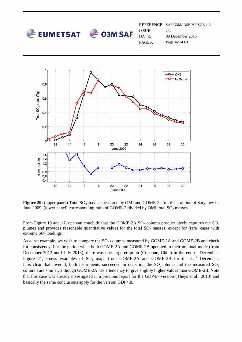
As a second case study, Figure 20 shows a comparison between the total SO2 mass time series of GOME-2

and OMI for the eruption of Sarychev, Russia, in June 2009. For this case, the saturation issue of GOME-2 is

less pronounced than for Kasatochi and happens only occasionally (e.g., 17 June). A striking feature of

Figure 20 is that GOME-2 retrievals are higher than OMI at the beginning of the eruption (12-15 June 2009).

This is related to the data filtering of OMI for the row anomaly which became stronger in 2009 compared to

2008 (Figure 19). Overall, one can conclude from Figure 19 that OMI and GOME-2 agree fairly well (e.g.,

within 20% for 20-30 June), in line with Figure 19.

REFERENCE:

ISSUE:

DATE:

PAGES:


1/1

09 December 2015

of 61

Figure 20: (upper panel) Total SO2 masses measured by OMI and GOME-2 after the eruption of Sarychev in

June 2009, (lower panel) corresponding ratio of GOME-2 divided by OMI total SO2 masses.

From Figure 19 and 17, one can conclude that the GOME-2A SO2 column product nicely captures the SO2

plumes and provides reasonable quantitative values for the total SO2 masses, except for (rare) cases with

extreme SO2 loadings.

As a last example, we wish to compare the SO2 columns measured by GOME-2A and GOME-2B and check

for consistency. For the period when both GOME-2A and GOME-2B operated in their nominal mode (from

December 2012 until July 2013), there was one large eruption (Copahue, Chile) in the end of December.

Figure 21, shows examples of SO2 maps from GOME-2A and GOME-2B for the 24th December.

It is clear that, overall, both instruments succeeded in detection the SO2 plume and the measured SO2

columns are similar, although GOME-2A has a tendency to give slightly higher values than GOME-2B. Note

that this case was already investigated in a previous report for the GDP4.7 version (Theys et al., 2013) and

basically the same conclusions apply for the version GDP4.8.

REFERENCE:

ISSUE:

DATE:

PAGES:


1/1

09 December 2015

of 61

Figure 21: Example of SO2 vertical columns for the December 24, 2012, as measured by GOME-2A (left)

and GOME-2B (right).

C.2.2 Investigating the case for anthropogenic SO2

As a first step, we evaluate the new data set for its ability to detect the large anthropogenic emissions sources

using global yearly SO2 maps of background corrected slant columns. Figure 22 shows examples for GOME-

2A in 2007 (beginning of operations) and both GOME-2A and GOME–2B for 2013. For these maps, no

cloud filtering was applied. Only the pixels selection criteria on SZA, viewing mode, flag and index in scan

have been used.

REFERENCE:

ISSUE:

DATE:

PAGES:


1/1

09 December 2015

of 61

REFERENCE:

ISSUE:

DATE:

PAGES:


1/1

09 December 2015

of 61

Figure 22: Yearly averaged SO2 slant columns averaged background from GOME-2A (top panel: 2007,

middle panel: 2013) and GOME-2B (lower panel: 2013). Only data corresponding to solar zenith angles

lower than 70° are shown. Note that the color scale of the column maps has been chosen in a way that all

features (including negative columns) can be best visualized.

Several remarks can be made, mostly in line with the results of Section C1:

1. A number of emission hotspots can be identified, in agreement with previous work of Fioletov et al.

(2013). In addition to some well-known degassing volcanoes, an SO2 signal from pollution is clearly

detected over China, Norilsk, South Africa, Eastern Europe and US (in 2007 only) and Middle East

(oil industry).

2. Several artifacts are also apparent in Figure 22:

a. At high latitudes, a general tendency to produce negative columns is observed for GOME-2A.

This problem is even more pronounced for GOME-2B at Northern high latitudes while positive

SO2 columns can be seen in the Antarctic region (notably for coastal areas). We note however

most of the available SO2 products have limitations at high latitudes (Fioletov et al., 2013). A

striking feature as well is found over the Hudson Bay where elevated values of SO2 are found in

both GOME-2A and –B datasets. The reason for this artifact is unknown but might be related to

a weather pattern there leading to lower tropopauses (hence higher O3 columns).

b. Both GOME-2A and –B SO2 column products are very sensitive to the South Atlantic Anomaly,

SAA and for that reason we recommend the application of a spike removal correction, see

Richter et al., 2011. For 2013, one can see that GOME-2A is dramatically affected by this issue.

The reason for this is related to the use of the inverse of the Earthshine radiance in the intensity

offset correction (see discussion in Section C1).

It is also clear from Figure 22 (middle panel) that the background SO2 levels outside the SAA

region are generally negative and it is unclear why that is the case.

REFERENCE:

ISSUE:

DATE:

PAGES:


1/1

09 December 2015

of 61

Figure 23 shows another example of comparison between results from GOME-2A and OMI (Theys et al.,

2015) for the year 2007 over China. To produce these SO2 maps, clear-sky pixels with cloud fractions less

than 30% have been selected and a fixed AMF of 0.4 (typical for a boundary layer SO2 profile) has been

applied to the background corrected slant columns, both for GOME-2 and OMI.

Figure 23: SO2 vertical columns (DU) averaged for 2007 for clear-sky pixels (cloud fraction

less than 0.3) for the GOME-2A (top panel) and OMI (bottom panel) instruments.

REFERENCE:

ISSUE:

DATE:

PAGES:


1/1

09 December 2015

of 61

Although the GOME-2 data are more noisy than OMI and some emissions spots are not detected by GOME-

2, one can see that, at first glance, similar patterns are observed by both sensors in Eastern China and that the

absolute values are comparable, with GOME-2 having a general tendency to produce higher values.

C.2.2.1 Comparison with MAX-DOAS measurements at Xianghe

The multi-axis DOAS instrument at Xianghe is a system developed by BIRA-IASB, and operated by the

Institute of Atmospheric Physics (IAP), Chinese Academy of Sciences. The description of the retrieval

technique and presentation of the results, including validation against in-situ measurements, can be found in

Wang et al. (2014). The SO2 profiles data set covers the period March 2010 until December 2013 and has

been used in Theys et al. (2015) to validate BIRA-IASB OMI SO2 columns.

Here we aim at validating the GOME-2 SO2 columns for the new GDP4.8 profile called 1km (which is also

used for the NASA OMI SO2 operational product (Li et al., 2013)), representing the scenario of

anthropogenic SO2 emissions (Taubmann et al., 2006).

The comparison between the ground-based and GOME-2 SO2 columns is done as follows: first, all GOME-2

(A and B separately) clear-sky pixels (i.e., cloud fractions less than 0.3) within a 150 km circle radius around

Xianghe and surface height less than 500 m (to exclude observations over clean elevated regions) with solar

zenith angles less than 70° are selected (in addition to the recommended pixel selection criteria, like viewing

mode, index in scan, etc.). Then, for each pixel, all MAX-DOAS data within ± 90 minutes of the GOME-

2 overpass time are considered and averaged for the comparison. In contrast to the OMI validation, we have

not corrected the GOME-2 SO2 columns using the MAX-DOAS mean SO2 profile. Doing so would allow (in

principle) a consistent comparison between MAX-DOAS and GOME-2 SO2 VCDs, but unfortunately the

information on averaging kernels (needed for this step) is not provided in the GOME-2 L2 files. We have not

attempted to recalculate AMFs using the BIRA-IASB tools because there are probably differences with the

approach and settings used in the operational processing environment.

Figure 24 shows the comparison between the monthly averaged ground-based (black dots) and coincident

GOME-2A SO2 columns for the period 03.2010-12.2013, at Xianghe.

We have considered both SO2 vertical columns using total AMFs (cyan) and clear-sky AMFs (red).

One can see that generally the MAX-DOAS and GOME-2 columns agree reasonably well and the seasonal

cycle of SO2 is consistent in both datasets. Among the two GOME-2 estimations, the results using the clear-

sky AMFs are in a better agreement with the MAXDOAS values than the retrievals based on total AMFs.

We note also that the cloud corrected values (using total AMFs) are always lower than the uncorrected ones

and the reason for this is because of the absence of a “ghost” (below cloud) column correction. One can

argue whether a cloud correction should be applied or not (given the uncertainties on cloud retrievals and a-

priori profiles) but if it is the case then a ghost correction should be included (as it is the case for other

GOME-2 trace gas products, such as NO2 and HCHO). In Figure 24 bottom panel, the differences between

GOME-2A (clear-sky) and MAX-DOAS columns are shown. As discussed before the agreement is

reasonably good especially for non-winter periods and the product reaches often the target/optimal accuracy

(50%/30%) and the threshold accuracy (100%) otherwise. Nevertheless, from Figure 24, it is not possible to

really consolidate these results because only one a-priori profile has been used for GOME-2 AMF

calculation for the whole time series, which is arguably a crude assumption.

A striking feature in Figure 24 is also a general positive trend in the differences (GOME-2A vs MAXDOAS)

and the reason for this anomaly will be investigated in the next section.

REFERENCE:

ISSUE:

DATE:

PAGES:


1/1

09 December 2015

of 61

We have estimated the relevant statistical parameters of the bi-variate linear regression GOME-2A clear-sky

columns versus MAX-DOAS (the scatter plot is shown on Figure 25). The correlation coefficient is equal to

0.64 and the slope of the linear regression fit is 1.23.

Figure 24: (top) Comparison of monthly averaged SO2 columns at Xianghe for the period 2010-

2013 measured by the MAX-DOAS and GOME-2A (using the anthropogenic SO2 emissions

profile). Two assumptions are made for the GOME-2 AMFs: total AMFs (in cyan) and clear-

sky AMFs (in red), (bottom) Time series of the SO2 column differences between GOME-2A

(using clear-sky AMFs) and MAXDOAS.

REFERENCE:

ISSUE:

DATE:

PAGES:


1/1

09 December 2015

of 61

Figure 25: Scatter plot of GOME-2A SO2 columns (calculated using clear-sky AMFs) versus MAX-DOAS

SO2 columns. Statistical parameters (correlation coefficient and slope of the linear regression (red line)) are

given inset. The black line is the 1:1 line.

Figure 26 and 24 are the equivalent comparison results for GOME-2B for the year 2013. Generally the same

findings as for GOME-2A also apply for GOME-2B: (a) SO2 columns using clear-sky AMFs are larger than

for total AMFs and are in a better agreement with the MAX-DOAS retrievals, (b) the GOME-2B (clear-sky)

SO2 columns are close to the MAXDOAS values except for winter. From Figure 27, the correlation

coefficient is equal to 0.55 and the slope of the linear regression (GOME-2B clear-sky columns versus

MAX-DOAS) fit is 1.49. However, we should be noted that these statistical parameters are significantly

influenced by two outlier points.

REFERENCE:

ISSUE:

DATE:

PAGES:


1/1

09 December 2015

of 61

REFERENCE:

ISSUE:

DATE:

PAGES:


1/1

09 December 2015

of 61

Figure 26: (top) Comparison of monthly averaged SO2 columns at Xianghe for the year 2013 measured by

the MAX-DOAS and GOME-2B (using the anthropogenic SO2 emissions profile). Two assumptions are

made for the GOME-2 AMFs: total AMFs (in cyan) and clear-sky AMFs (in red), (bottom) Time series of

the SO2 column differences between GOME-2B (using clear-sky AMFs) and MAXDOAS.

Figure 27: Scatter plot of GOME-2B SO2 columns (calculated using clear-sky AMFs) versus MAX-DOAS

SO2 columns. Statistical parameters (correlation coefficient and slope of the linear regression (red line)) are

given inset. The black line is the 1:1 line.

C.2.2.2 Stability of the GOME-2A and –B SO2 column products as a function of time

Figure 28 shows time-series of SO2 SCDs over the Equatorial Pacific averaged on a monthly basis for the

GOME-2A and GOME-2B periods, and for different ranges of Line-of-Sight (LOS) angles (LOS<20°,

20°<=LOS<40°, LOS>=40°).

For GOME-2A, one can see that the SCD values are rather small at the beginning of the mission and then

rapidly increase until beginning of 2009 when a strong decrease of the SCDs occurs. After the GOME-2A

throughput test, the SCD values for the different LOS start to deviate significantly from each other, with

absolute differences between low and high viewing angles up to 0.25 DU. We also notice an important

negative trend in the SCDs from 2011 onwards. After July 2013, GOME-2A is in its reduced swath mode

(hence no high LOS data) and the SCDs for low and medium LOS come closer to zero.

We interpret the behavior depicted in Figure 28 (top panel) as related to the time evolution of the shape of

the instrumental slit function in the wavelength range used to retrieve SO2. The actual slit function shape

deviates quite quickly and significantly from the slit function characterized before the launch (and used in

the DOAS fit of SO2). A plausible impact on the spectral fitting is a reinforcement of the interference with

ozone and this probably explains the erratic LOS dependence of the SCDs (the background correction

REFERENCE:

ISSUE:

DATE:

PAGES:


1/1

09 December 2015

of 61

applied to the retrieved SCDs do not account for dependences neither on LOS nor on ozone absorption).

Note that this effect is not limited to SO2, and e.g. De Smedt et al. (2012) studied the impact of slit function

changes on GOME-2 HCHO retrievals and implemented an improved procedure consisting in fitting

asymmetric slit function parameters as part of the HCHO DOAS inversion.

For SO2, several tests have been done as well and the BIRA-IASB Scientific GOME-2 SO2 algorithm

currently uses the shape of the slit function characterized before launch but allows for shift and stretch of the

slit function during the DOAS process. Moreover, a background correction depending on LOS and measured

ozone slant column is also applied. For the sake of completeness, we show in Figure 29 the results of the

BIRA-IASB GOME-2A SO2 product (but limited to the year 2010) and one can see that the problem in

Figure 28 (top panel) is largely resolved.

REFERENCE:

ISSUE:

DATE:

PAGES:


1/1

09 December 2015

of 61

Figure 28: Time-series of monthly averaged SO2 background corrected slant columns over the Equatorial

pacific (10°S-10°N, 160°E-120°W) for different ranges of line-of-sight angles, for GOME-2A (upper panel)

and GOME-2B (lower panel).

REFERENCE:

ISSUE:

DATE:

PAGES:


1/1

09 December 2015

of 61

Figure 29: same as Figure 28 (upper panel) for the BIRA-IASB GOME-2A SO2 product for the year 2010.

For GOME-2B, the results of Figure 28 (bottom panel) reveal a very strong LOS dependence of the SO2

SCDs but relatively stable over time. This suggests an alteration of the slit function shape (relative to pre-

launch slit function) already from the very start of the GOME-2B operations.

The same investigations have been performed at other places and Figure 30 shows, as an example, the results

for Xianghe. Note that for the GOME-2A data (Figure 30, upper panel), only yearly averages are displayed

(rather than monthly averages as in Figure 28), because the corresponding graph with monthly averaged

values was found difficult to read (because of strong SO2 variability at Xianghe), but it is does not change the

overall conclusion.

REFERENCE:

ISSUE:

DATE:

PAGES:


1/1

09 December 2015

of 61

REFERENCE:

ISSUE:

DATE:

PAGES:


1/1

09 December 2015

of 61

Figure 30: same as Figure 28, for the pixels within a 150 km circle radius around Xianghe. (top panel)

GOME-2A yearly SO2 SCD averages, (bottom panel) GOME-2B monthly SO2 SCD averages.

It is obvious from Figure 30 that the LOS dependence over the Equatorial Pacific (Figure 28) is also clearly

seen over Xianghe (both for GOME-2A and –B). If one consider the year 2010 (GOME-2A) for instance, the

absolute difference in slant columns between the low and high LOS is up to ~0.25 DU. If ones assumes a

typical AMF of 0.45-0.5 for a polluted scene (see Figure 13 of the SO2 ATBD; Valks et al., 2015), this

translates into an error on the SO2 vertical columns of 0.5-0.55 DU (and more in winter). For GOME-2B, this

effect is even larger (the corresponding error on the vertical columns is easily higher than 1 DU). We

recommend to further work on this issue to gain confidence in the data and its evolution with time.

REFERENCE:

ISSUE:

DATE:

PAGES:


1/1

09 December 2015

of 61

D. CONCLUSIONS

This document reports on the validation of NRT, offline and reprocessed GOME-2A and -B SO2 column

data products retrieved at DLR with versions 4.8 of the GOME Data Processor (GDP), using level-1B

data based on the level-0-1B processor version 5.x and 6.0.

Compared to the previous data version, the new GDP4.8 SO2 product has three new important and

notable features: (a) consistent retrieval settings have been applied to both GOME-2A and GOME-2B

sensors, (b) a boundary layer SO2 product, similar to the PBL OMI/Aura product, has been introduced

and (c) a volcanic flag has been implemented.

GOME-2A & B SO2 vertical columns have been evaluated using (1) comparisons with previous version

(4.7) of the algorithm and by assessing the consistency between the two sensors (for GDP4.8 version),

(2) comparisons with correlative data sets from OMI (PCA and DOAS algorithms) and MAX-DOAS

measurements at Xianghe, China.

Note that the conclusions are based on the original GDP4.8 dataset made available to the validation team in

late May 2015. Following the first results of the validation process which were made available to the

operational team, a suite of new GDP4.8 algorithm test runs were performed for years 2008 and 2013 that

could solve some of the issues identified hereafter.

The following main conclusions can be drawn:

Comparison of GDP4.7 and GDP4.8: For the slant columns, there are negligible differences between

the two versions for GOME-2B while for GOME-2A the slant columns show some differences. An

important feature in GOME-2A is a stronger effect of the South Atlantic Anomaly (see below). For

the vertical columns, the data are found to be noisier in the new version and the GOME-2A GDP4.8

2.5km plume height product shows between 0 and 0.5-1 D.U. higher SO2 loading on a yearly basis

than the GDP4.7 algorithm, whereas for GOME-2B this increase is smaller, between 0 and 0.5 D.U.

at the known hot spots. Retrievals tests have shown that this was due to the use of the inverse of the

Earthshine spectrum in the DOAS intensity offset correction; this issue is largely solved by using

instead the inverse of the Solar spectrum. This setting is the new baseline for the GDP4.8 SO2

algorithm.

GOME-2A- GOME-2B-OMI consistency: 33 known SO2 emitting locations around the world,

including volcanoes, power plants, smelters, and so on, were used to compare the GOME-2A and -

2B SO2 to the OMI estimates. The average SO2 loading of these sources was 0.41±0.31 D.U. for

GOME-2A, 0.08±0.24 D.U. for GOME-2B and 0.30±0.31 D.U. for OMI. GOME-2A was found to

be in better agreement with OMI than GOME-2B GDP4.8 due to the higher amount of negative

mean loadings shown by the newer instrument. However, the mean correlation coefficient for these

sites between GOME2 and OMI was found to be 0.42 for GOME-2A and 0.51 for GOME-2B

pointing to the fact that both GOME-2A and –2B GDP 4.8 SO2 column retrievals fare well with

OMI/Aura considering all the limitations.

Volcanic SO2: GOME-2A and –B GDP 4.8 SO2 column retrievals is clearly able to capture and track

plumes after small to strong eruptions, but the newly implemented flag for volcanic SO2 misses parts

of aged and filamentary plumes. Quantitatively, the SO2 masses estimated from GOME-2 after

strong eruptions agree very well with OMI (with differences mostly within the 30% optimal

accuracy), except for the rather unusual very high SO2 amounts (for the first days after the start of the

eruption) where GOME-2 underestimates the columns (saturation effect).

REFERENCE:

ISSUE:

DATE:

PAGES:


1/1

09 December 2015

of 61

Anthropogenic SO2: the addition of a new SO2 column in GDP4.8 using a typical profile for

anthropogenic emissions scenario is an improvement and allows direct comparison with OMI. From

comparisons with OMI, it can be concluded that 1) several hotspots are seen by both satellite

datasets and the mean values from GOME-2 and OMI are reasonably close, 2) some weak emissions

are not detected by GOME-2, partly because of the better spatial resolution of OMI but also because

GOME-2 data is more noisy. From the comparison (using the anthropogenic SO2 column field) with

the MAXDOAS-data, the best agreement is found for the results using clear-sky AMFs (while the

results for total AMFs are always found lower). The agreement is reasonably good especially for

non-winter periods and the product reaches often the target/optimal accuracy (50%/30%) and the

threshold accuracy (100%) otherwise.

Localized artefacts and product self-inconsistency: Several artefacts are found in the maps e.g. at

high latitudes. Over the SAA region specifically, the GOME-2 data shows a dramatic trend over time

with noisy and elevated SO2 columns over the last years (this effect is worst in GDP4.8 than

GDP4.7). This feature is due to the treatment of the DOAS intensity offset correction An

investigation of the SO2 SCDs over clean and polluted regions shows an anomalous dependence of

the results with viewing angles for both sensors. The most likely explanation for this effect is due to

differences between the slit functions used in the spectral fitting (extracted from the GOME-2 key

data) and the actual ones.

REFERENCE:

ISSUE:

DATE:

PAGES:


1/1

09 December 2015

of 61

E. REFERENCES

E.1 Applicable documents

[ATBD] Algorithm Theoretical Basis Document for GOME-2 Total Column Products of Ozone,

NO2, BrO, SO2, H2O, HCHO and Cloud Properties (GDP 4.8 for O3M-SAF OTO and

NTO), DLR/GOME-2/ATBD/01, Rev. 3/A, Valks, P., et al., March 2015.

[PUM] Product User Manual for GOME-2 Total Column Products of Ozone, NO2, BrO, SO2, H2O,

HCHO and Cloud Properties, DLR/GOME-2/PUM/01, Rev. 3/A, Valks, P., et. al., 2015.

[PRD] Product Requirements Document, SAF/O3M/FMI/RQ/PRD/001/Rev. 1.7, D. Hovila, S.

Hassinen, D. Loyola, P. Valks, J., S. Kiemle, O. Tuinder, H. Joench-Soerensen, F. Karcher,

2015.

E.2 Reference documents

E.2.1 Peer-reviewed articles

Bogumil, K., J. Orphal, T. Homann, S. Voigt, P. Spietz, O.C. Fleischmann, A. Vogel, M. Hartmann, H.

Kromminga, H. Bovensmann, J. Frerick, J.P. Burrows (2003), Measurements of molecular absorption spectra

with the SCIAMACHY pre-flight model: instrument characterization and reference data for atmospheric

remote-sensing in the 230-2380nm region, Journal of Photochemistry and Photobiology, A:Chemistry, 157 ,

167-184.

Brenot, H., Theys, N., Clarisse, L., van Geffen, J., van Gent, J., Van Roozendael, M., van der A, R.,

Hurtmans, D., Coheur, P.-F., Clerbaux, C., Valks, P., Hedelt, P., Prata, F., Rasson, O., Sievers, K., and

Zehner, C.: Support to Aviation Control Service (SACS): an online service for near real-time satellite

monitoring of volcanic plumes, Nat. Hazards Earth Syst. Sci., 14, 1099-1123, doi:10.5194/nhess-14-1099-

2014, 2014.

Brion, J., et al.: Absorption spectra measurements for the ozone molecule in the 350-830 nm region, J.

Atmos. Chem., 30, 291-299, 1998.

Carn, S. A., A. J. Krueger, N. A. Krotkov, K. Yang, and P. F. Levelt (2007a), Sulfur dioxide emissions from

Peruvian copper smelters detected by the Ozone Monitoring Instrument, Geophys. Res. Lett., 34, L09801,

doi:10.1029/2006GL029020.

Carn, S.A., N.A. Krotkov, K. Yang, R.M. Hoff, A.J. Prata, A.J. Krueger, S.C. Loughlin, and P.F. Levelt

(2007b), Extended observations of volcanic SO2 and sulfate aerosol in the stratosphere, Atmos. Chem. Phys.

Discuss., 7, 2857-2871. (http://www.atmos-chem-phys-discuss.net/7/2857/2007/acpd-7-2857-2007.html)

Carn, S.A., A.J. Krueger, N.A. Krotkov, S. Arellano, and K. Yang (2008a), Daily monitoring of Ecuadorian

volcanic degassing from space, J. Volcanol. Geotherm. Res., (in press).

Carn, S.A., A.J. Krueger, N.A. Krotkov, K. Yang, and K. Evans (2008b), Tracking volcanic sulfur dioxide

clouds for aviation hazard mitigation. Natural Hazards, Special Issue on Aviation Hazards from Volcanoes

(in press).

http://www.atmos-chem-phys-discuss.net/7/2857/2007/acpd-7-2857-2007.html

REFERENCE:

ISSUE:

DATE:

PAGES:


1/1

09 December 2015

of 61

Clarisse, L., Hurtmans, D., Clerbaux, C., Hadji-Lazaro, J., Ngadi, Y., and Coheur, P.-F.: Retrieval of

sulphur dioxide from the infrared atmospheric sounding interferometer (IASI), Atmos. Meas. Tech., 5, 581-

594, 2012.

De Smedt, I., Van Roozendael, M., Stavrakou, T., Müller, J.-F., Lerot, C., Theys, N., Valks, P., Hao, N., and

van der A, R.: Improved retrieval of global tropospheric formaldehyde columns from GOME-2/MetOp-A

addressing noise reduction and instrumental degradation issues, Atmos. Meas. Tech., 5, 2933-2949,

doi:10.5194/amt-5-2933-2012, 2012.

Fioletov, V. E., C. A. McLinden, N. Krotkov, K. Yang, D. G. Loyola, P. Valks,

N. Theys, M. Van Roozendael, C. R. Nowlan, K. Chance, X. Liu, C. Lee,

and R. V. Martin: Application of OMI, SCIAMACHY, and GOME-2 satellite SO2 retrievals for detection of

large emission sources, J. Geophys. Res. Atmos., 118, 11,399–11,418, doi:10.1002/jgrd.50826, 2013.

Gür, B., P. Spietz, J. Orphal, and J. Burrows (2005), Absorption spectra measurements with the GOME-2

FMs using the IUP/IFE-UB’s calibration apparatus for trace gas absorption spectroscopy CATGAS, final

report, Inst. of Environ. Phys., Univ. of Bremen, Bremen, Germany.

Krotkov, N.A., B. McClure, R.R. Dickerson, S.A. Carn, C. Li, P.K. Bhartia, K. Yang, A.J. Krueger, Z. Li, P.F.

Levelt, H. Chen, P. Wang and D. Lu, Validation of SO2 retrievals from the Ozone Monitoring Instrument

over NE China, J. Geophys. Res., 2008, 113, doi:10.1029/2007JD008818.

Krotkov, N.A., S.A. Carn, A.J. Krueger, P.K. Bhartia, and K. Yang (2006). Band residual difference

algorithm for retrieval of SO2 from the Aura Ozone Monitoring Instrument (OMI). IEEE Trans.Geosci.

Remote Sensing, AURA special issue, 44(5), 1259-1266, doi:10.1109/TGRS.2005.861932, 2006

Krueger, A.J., L.S. Walter, P.K. Bhartia, C.C. Schnetzler, N.A. Krotkov, I. Sprod, and G.J.S. Bluth (1995)

Volcanic sulfur dioxide measurements from the total ozone mapping spectrometer instruments. J. Geophys.

Res., 100(D7), 14057-14076, 10.1029/95JD01222.

Krueger, A., Krotkov, N. and Yang, K., “Comparison of GOME-2 and OMI sulfur dioxide retrievals”,

Atmospheric Science Conference Barcelona, Spain, 7-11 September 2009.

Li, C., J. Joiner, N. A. Krotkov, and P. K. Bhartia (2013), A fast and sensitive new satellite SO2 retrieval

algorithm based on principal component analysis: Application to the ozone monitoring instrument, Geophys.

Res. Lett., 40, 6314–6318, doi:10.1002/2013GL058134.

Puķīte, J., Kühl, S., Deutschmann, T., Platt, U., and Wagner, T.: Extending differential optical absorption

spectroscopy for limb measurements in the UV, Atmos. Meas. Tech., 3, 631-653, 2010.

Richter, A., M. Begoin, A. Hilboll, and J. P. Burrows (2011), An improved NO2 retrieval for the GOME-2

satellite instrument, Atmos. Meas. Tech., 4, 1147–1159, doi:10.5194/amt-4-1147-2011.

Rix, M., Valks, P., Hao, N., Loyola, D. G., Schlager, H., Huntrieser, H. H., Flemming, J., Koehler,

U., Schumann, U., and Inness, A.: Volcanic SO2, BrO and plume height estimations using GOME-2

satellite measurements during the eruption of Eyjafjallajökull in May 2010, J. Geophys. Res., 117,

D00U19, doi:10.1029/2011JD016718, 2012.

SACS, Support to Aviation Control Service, SO2 maps available in near-real-time at

http://sacs.aeronomie.be.

http://sacs.aeronomie.be/

REFERENCE:

ISSUE:

DATE:

PAGES:


1/1

09 December 2015

of 61

Spurr, R. J. D., T. P. Kurosu, and K. V. Chance: A Linearized discrete Ordinate Radiative Transfer Model

for Atmospheric Remote Sensing Retrieval, J. Quant. Spectrosc. Radiat. Transfer, 68, 689-735, 2001.

Taubman, B. F., J. C. Hains, A. M. Thompson, L. T. Marufu, B. G. Doddridge, J. W. Stehr, C. A. Piety, and

R. R. Dickerson (2006), Aircraft vertical profiles of trace gas and aerosol pollution over the mid- Atlantic

United States: Statistics and meteorological cluster analysis, J. Geophys. Res., 111, D10S07,

doi:10.1029/2005JD006196.

Theys, N., I. De Smedt, J. van Gent, T. Danckaert, T. Wang, F. Hendrick, T. Stavrakou, S. Bauduin, L.

Clarisse, C. Li, N. A. Krotkov, H. Yu, M. Van Roozendael, Sulfur dioxide vertical column DOAS retrievals

from the Ozone Monitoring Instrument: Global observations and comparison to ground‐based and satellite

data, J. Geophys. Res. Atmos., 120, doi:10.1002/2014JD022657, 2015.

Walker, J. C., E. Carboni, A. Dudhia, and R. G. Grainger (2012), Improved detection of sulphur dioxide in

volcanic plumes using satellite-based hyperspectral infrared measurements: Application to the

Eyjafjallajökull 2010 eruption, J. Geophys. Res., 117, D00U16, doi:10.1029/2011JD016810.

Wang, T., Hendrick, F., Wang, P., Tang, G., Clémer, K., Yu, H., Fayt, C., Hermans, C., Gielen, C.,

Müller, J.-F., Pinardi, G., Theys, N., Brenot, H., and Van Roozendael, M.: Evaluation of tropospheric SO2

retrieved from MAX-DOAS measurements in Xianghe, China, Atmos. Chem. Phys., 14, 11149-11164,

doi:10.5194/acp-14-11149-2014, 2014.

Yang, K., N. Krotkov, A. Krueger, S. Carn, P. K. Bhartia, and P. Levelt (2007), Retrieval of Large Volcanic

SO2 columns from the Aura Ozone Monitoring Instrument (OMI): Comparisons and Limitations, J. Geophys.

Res., 112, D24S43, doi:10.1029/2007JD008825

E.2.2 Technical notes

Theys et al., 2013, OM3SAF SO2 validation report, TN-IASB-GOME-2B-O3MSAF-SO2-2013.

van Geffen, J., Van Roozendael, M., Rix, M., Valks, P.: Initial validation of GOME-2 GDP 4.2 SO2 total

columns (OTO/SO2) – ORR B, O3MSAF validation report, TN IASB-GOME2-O3MSAF-SO2-01.1, 2008.

Valks et al., 2015 ; Algorithm Theoretical Basis Document for GOME-2 Total Column Products of Ozone,

NO2, BrO, HCHO, SO2, H2O and Cloud Properties (GDP 4.8 for O3M-SAF OTO and NTO), DLR/GOME-

2/ATBD/01/3/A

o3m saf validation report - acsaf.org · function organisation o3m-saf eumetsat, bira-iasb, dlr,...

Documents