nvh lecture 7: operational modal analysis · time animation – operational deflection shapes ......
TRANSCRIPT
Copyright LMS International 1
Marie Curie Graduate School on Vehicle Mechatronics & Dynamics, Leuven, 5-8 February 2013 Bart Peeters
NVH Lecture 7: Operational Modal Analysis
2 copyright LMS International - 2011
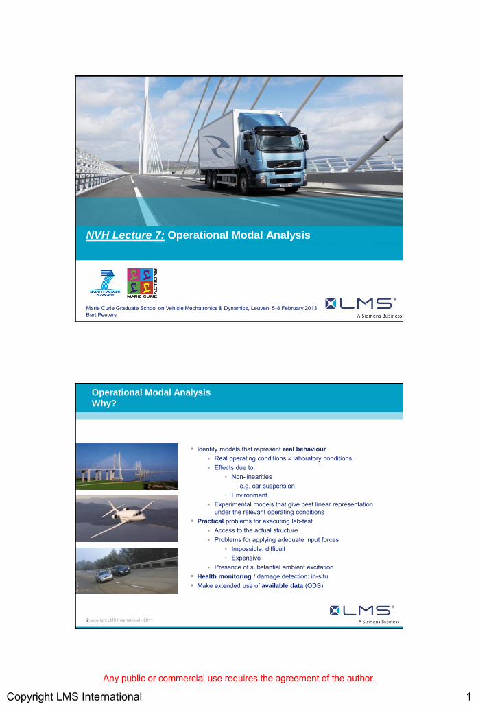
Operational Modal Analysis
Why?
Identify models that represent real behaviour
Real operating conditions laboratory conditions Effects due to:
• Non-linearities e.g. car suspension
• Environment Experimental models that give best linear representation
under the relevant operating conditions Practical problems for executing lab-test
Access to the actual structure Problems for applying adequate input forces
• Impossible, difficult • Expensive
Presence of substantial ambient excitation Health monitoring / damage detection: in-situ Make extended use of available data (ODS)
Any public or commercial use requires the agreement of the author.

Copyright LMS International 2
3 copyright LMS International - 2011
Operational Modal Analysis
In-operation testing
Some applications permit the use of Input - output (FRF) data during normal operation
Require special setups for forced excitation • Rotating wing-tip vanes • Electromagnetic bearings • Low-frequency exciters • Drop-weights • Unbalance shakers • Pyrotechnics • Control Surface Input • Servo-drive inputs (robots) • …
Testing complexity Data quality (undesired ambient sources)
Some applications permit simulating in-operation
conditions in I/O (FRF) tests (car suspension…) The normal EMA processes can be followed
© NASA
© EMPA © KUL
4 copyright LMS International - 2011
In-operation EMA example:
Business jet, wing-vane in-flight excitation
In-flight excitation, 2 wing-tip vanes 9 responses 2 min sine sweep Higher order harmonics Very noisy data
4.00 20.00LinearHz
0.00
0.10
Log
(g/N
)
4.00 20.00LinearHz
Hz-180.00
180.00
Phas
e°
PolyMAX
4.00 20.00Linear
Hz
10.0e-6
1.00
Log
(m/s
2)/N
4.00 20.00LinearHz
Hz
-180.00
180.00
Phas
e°
Hz
0.05
1.00
Ampl
itude
/
Coherence w ing:vvd:+Z/MultipleCoherence back:vde:+Y/Multiple
Any public or commercial use requires the agreement of the author.

Copyright LMS International 3
5 copyright LMS International - 2011
Majority of applications: use of output-only data
Objective: Identification of modal parameters from output-
only data measured on a structure during standard operation. Eigenfrequency Damping Mode shape
Output-only operational modal analysis = identifying H
Based on Y
Without knowing U
Desired (but unknown) ambient sources: “white” spectrum
What is Operational Modal Analysis? Operational Modal Analysis
The output-only system identification problem
H U Y
Input System Output
6 copyright LMS International - 2011
Operational Modal Analysis
The output-only system identification problem
In the remainder, we will focus on output-only methods for in-operation modal analysis. We will refer to this as OMA
Operational Modal Analysis (= operational response modal analysis). In general (papers, software vendors, test procedures), OMA hence implies ―output-
only modal analysis‖
White noise
H U Y
White noise + harmonic Ideal operational excitation
Less ideal operational excitation
Any public or commercial use requires the agreement of the author.

Copyright LMS International 4
7 copyright LMS International - 2013
Operational Modal Analysis in the presence of rotating machinery
Sweeping harmonics (run-up) Harmonics excite broad frequency band Useful excitation – no filtering! ―End-of-order‖ effects
Fixed (or slowly varying) harmonics Harmonics hamper the identification
process Have to be removed from data
Helico
pte
r in
-flig
ht
data
C
ar
en
gin
e r
un
-up
8 copyright LMS International - 2011
Direct animation of signals in time
domain
Animation of Structures
Time Animation – Operational Deflection Shapes
Actual deformation as a function of time or frequency Explanation & model through modal analysis
Direct animation of frequency-domain
functions
Any public or commercial use requires the agreement of the author.

Copyright LMS International 5
9 copyright LMS International - 2011
Operational Modal Analysis
More than operational deflection shapes
Auto & Cross Powers
Peak picking
Deformation at a chosen frequency line
No damping information
Combination of modes and forced responses
Combination of closely spaced modes
Data reduction through coherence or SVD analysis (Principal Component Analysis)
Phenomena
Modal model Frequency Damping Mode shape (No modal scaling)
Use of system identification methods
Structural characteristics
Separation of closely spaced modes
Root causes
OMA ODS
Vibration problem “root cause” discriminator
10 copyright LMS International - 2011
OMA as part of an engineering workflow
Wind turbine operational testing
Component testing Classical Modal Analysis Validation of component models
Assembled structure testing Operational Modal Analysis Validation of assembly models
OCT 2 2003
PLOT NO. 2
NODAL SOLUTION
STEP=1
SUB =2
FREQ=32.423
USUM
TOP
RSYS=0
DMX =.065211
SMX =.065211
1
MN
MX
2
MN
MX
3
MN
MX
4
MN
MX
XY
Z
0
.007246
.014491
.021737
.028983
.036228
.043474
.05072
.057965
.065211
X
Y
Z
0
.007246
.014491
.021737
.028983
.036228
.043474
.05072
.057965
.065211
X Y
Z
0
.007246
X
YZ
FE MODEL
EMA MODEL
UPDATED
FE MODEL
Source: Laurent Bonnet, GE Energy
LMS Conference Europe, Nürburg, 2-3 March 2005
Any public or commercial use requires the agreement of the author.
Copyright LMS International 6
11 copyright LMS International - 2011
0.00 80.00 Hz10.0e-6
0.10
Log
(g/N
)
0.00 80.00 LinearHz
0.00 80.00 Hz-180.00
180.00
Phas
e°
0.00 6.00 s-1.07
0.91
Rea
l(g/
N
)
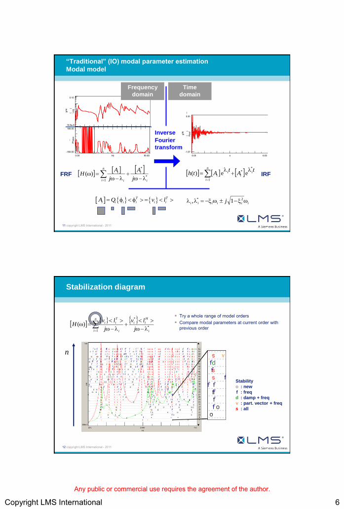
“Traditional” (IO) modal parameter estimation
Modal model
Inverse
Fourier
transform
Frequency
domain
Time
domain
FRF IRF
n
i i
i
i
i
j
A
j
AH
1*
*
)(
n
i
ii
ii
tA
tAth
1
** ee)(
T T
i i i i i iA Q v l iiiiii j 2* 1,
12 copyright LMS International - 2011
Stabilization diagram
Try a whole range of model orders Compare modal parameters at current order with
previous order
Stability
: new
: freq
: damp + freq
: part. vector + freq
: all
o
f
d
v
s
n
n
i i
H
ii
i
T
ii
j
lv
j
lvH
1*
*
)(
Any public or commercial use requires the agreement of the author.

Copyright LMS International 7
13 copyright LMS International - 2011
Stabilization diagram
? PolyMAX ! Model order problem shifted to problem of separating true from computational poles?
14 copyright LMS International - 2011
Operational
data
Preprocessing operational data
]DFT[window )()( s
k
s yY
Hsss
yy YYS )()()(
P
s
s
yyyy SP
S1
)( )(1
)(
2.00 8.00 Linear
Hz
1.00e-12
10.0e-9
Log
(m2/
s4
)
autopow er_spectr roof:1:+Z / roof:1:+Zcrosspow er_spect roof:1:+X / roof:1:+Z
2.00 8.00 LinearHz
2.00 8.00 Hz
-180.00
180.00
Phas
e°
ky
Periodogram (“classical”)
Periodogram
with
Hanning
window
1
0
1 N
k
Tkiki yy
NR
}],...,2/{DFT[window)( 0 Lyy RRS
2.00 8.00 Linear
Hz
1.00e-12
1.00e-9
Log
( m/s
2 )2
AutoPow er roof:1:+ZCrossPow er roof:1:+X/roof:1:+Z
2.00 8.00 LinearHz
2.00 8.00 Hz-180.00
180.00
Phas
e°
}],...,,...,{DFT[window)( 0 LLyy RRRS
Correlogram (“half spectra”)
Correlogram
with
exponential
window
Any public or commercial use requires the agreement of the author.
Copyright LMS International 8
15 copyright LMS International - 2011
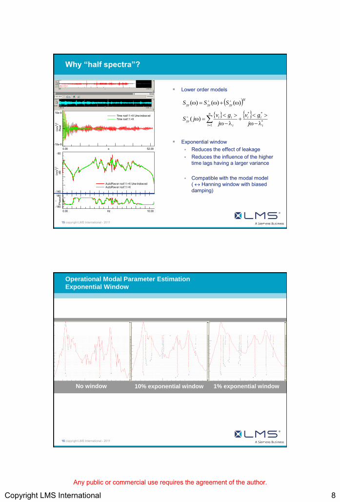
Why “half spectra”?
Lower order models
Exponential window Reduces the effect of leakage Reduces the influence of the higher
time lags having a larger variance
Compatible with the modal model ( Hanning window with biased damping)
Hyyyyyy SSS )()()(
n
i i
ii
i
iiyy
j
gv
j
gvjS
1*
**
)(
0.00 52.00 s-10e-9
10e-9
Rea
l( m
/s2 )2
Time roof:1:+X Unw indow edTime roof:1:+X
0.00 10.00 LinearHz
-140
-90
dB( m/s
2 )2
AutoPow er roof:1:+X Unw indow edAutoPow er roof:1:+X
0.00 10.00 LinearHz
0.00 10.00 Hz-180
180
Pha
se°
16 copyright LMS International - 2011
No window
Operational Modal Parameter Estimation
Exponential Window
10% exponential window 1% exponential window
Any public or commercial use requires the agreement of the author.
Copyright LMS International 9
17 copyright LMS International - 2011
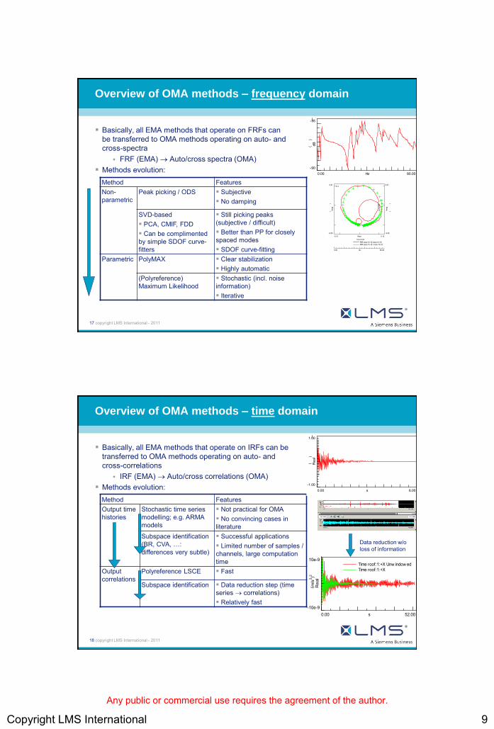
Overview of OMA methods – frequency domain
Basically, all EMA methods that operate on FRFs can be transferred to OMA methods operating on auto- and cross-spectra
FRF (EMA) Auto/cross spectra (OMA) Methods evolution:
0.00 80.00 Hz
-90
-35
dB(g/N
)
-0.13 0.13 Real((m/s2)/N)
-0.05
0.21
Imag
((m/s
2)/N
)
-0.05
0.21
Imag
((m/s
2)/N
)
0.00 50.00 Hz
1:1
FRF moto:15:+Z moto:15:+ZFRF moto:15:+Z / moto:15:+Z
Method Features Non-parametric
Peak picking / ODS Subjective No damping
SVD-based PCA, CMIF, FDD Can be complimented by simple SDOF curve-fitters
Still picking peaks (subjective / difficult) Better than PP for closely spaced modes SDOF curve-fitting
Parametric PolyMAX Clear stabilization Highly automatic
(Polyreference) Maximum Likelihood
Stochastic (incl. noise information) Iterative
18 copyright LMS International - 2011
0.00 52.00 s-10e-9
10e-9
Rea
l( m
/s2 )2
Time roof:1:+X Unw indow edTime roof:1:+X
Overview of OMA methods – time domain
Basically, all EMA methods that operate on IRFs can be transferred to OMA methods operating on auto- and cross-correlations
IRF (EMA) Auto/cross correlations (OMA) Methods evolution:
Method Features Output time histories
Stochastic time series modelling; e.g. ARMA models
Not practical for OMA No convincing cases in literature
Subspace identification (BR, CVA, …: differences very subtle)
Successful applications Limited number of samples / channels, large computation time
Output correlations
Polyreference LSCE Fast
Subspace identification Data reduction step (time series correlations) Relatively fast
0.00 6.00 s
-1.00
1.00
Rea
l(g/
N
)
Data reduction w/o loss of information
Any public or commercial use requires the agreement of the author.

Copyright LMS International 10
19 copyright LMS International - 2011
Case studies
Aerospace engineering Civil Engineering Automotive Engineering
20 copyright LMS International - 2011
Test – FEM correlation
Frequency correlations within 5%
FEM updating with ―delta stick‖ approach
Any public or commercial use requires the agreement of the author.
Copyright LMS International 11
21 copyright LMS International - 2011
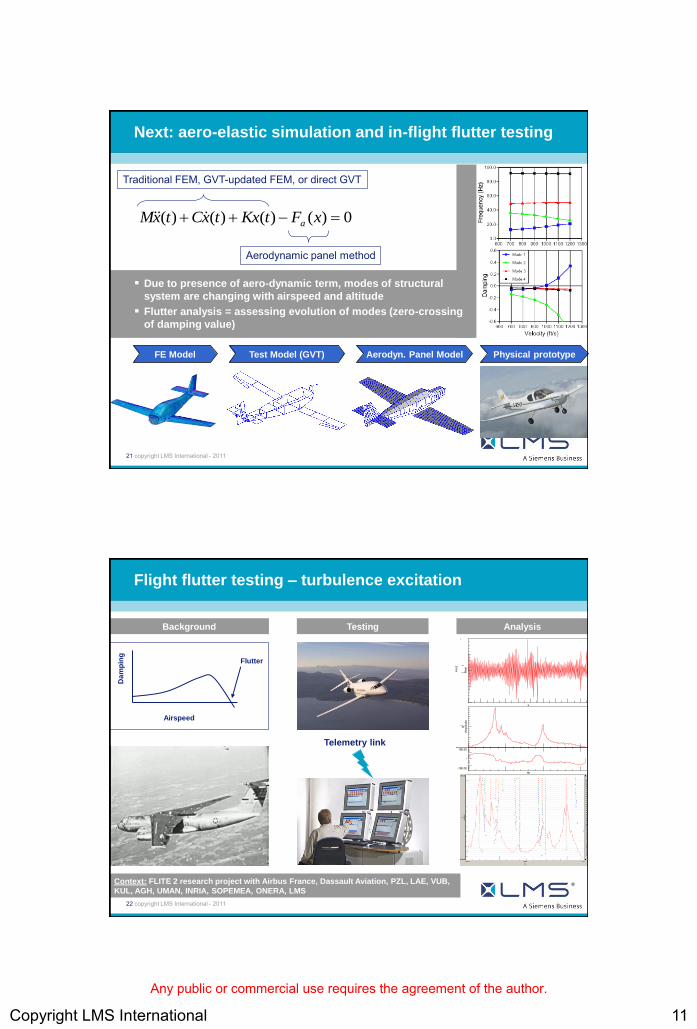
Next: aero-elastic simulation and in-flight flutter testing
FE Model Test Model (GVT) Aerodyn. Panel Model Physical prototype
0)()()()( xFtKxtxCtxM a
Traditional FEM, GVT-updated FEM, or direct GVT
Aerodynamic panel method
Due to presence of aero-dynamic term, modes of structural
system are changing with airspeed and altitude
Flutter analysis = assessing evolution of modes (zero-crossing
of damping value)
22 copyright LMS International - 2011
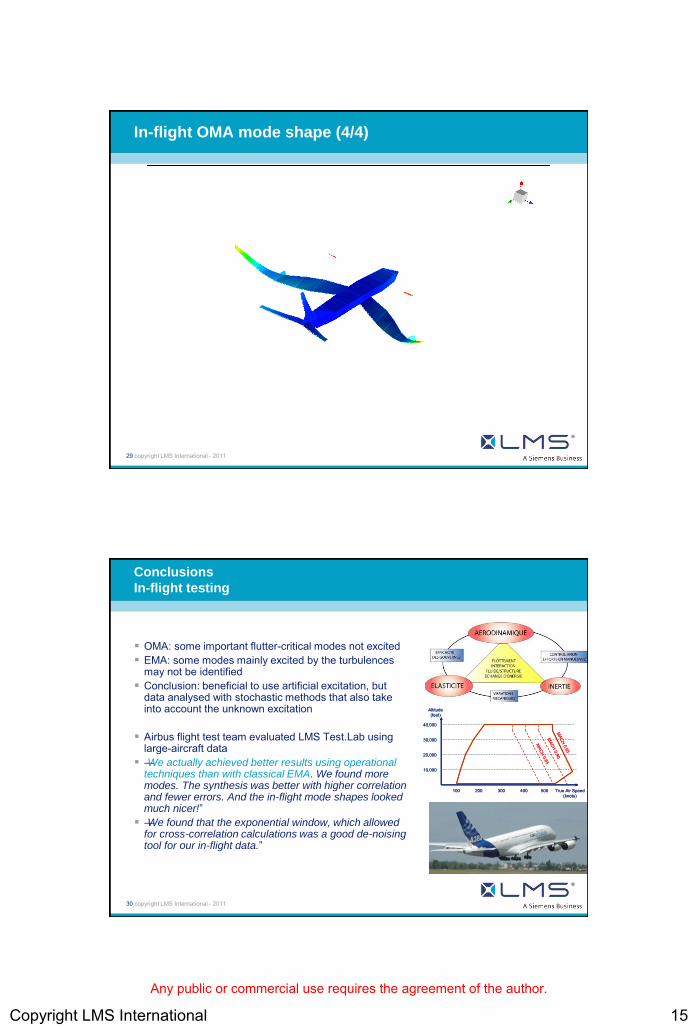
Flight flutter testing – turbulence excitation
s
Rea
l(m
/s2 )
0.00 3.20 LinearHz
Am
plitu
deg2
0.00 3.20 LinearHz
Hz-180.00
180.00
°
Da
mp
ing
Airspeed
Flutter
Telemetry link
Background Testing Analysis
Context: FLITE 2 research project with Airbus France, Dassault Aviation, PZL, LAE, VUB,
KUL, AGH, UMAN, INRIA, SOPEMEA, ONERA, LMS
Any public or commercial use requires the agreement of the author.

Copyright LMS International 12
23 copyright LMS International - 2011
Application to aircraft flight test data
Generally only a few sensors
24 copyright LMS International - 2011
A380 in-flight tests
But sometimes a bit more: 150 accelerometers
Any public or commercial use requires the agreement of the author.

Copyright LMS International 13
25 copyright LMS International - 2011
OMA – PolyMAX
0.71 6.05Linear
Hz
dB
Sum Crosspow er SUMSynthesized Crosspow er SUM0.71 6.05Linear
Hz
Hz-180.00
180.00
Phas
e°
26 copyright LMS International - 2011
In-flight OMA mode shape (1/4)
Any public or commercial use requires the agreement of the author.

Copyright LMS International 14
27 copyright LMS International - 2011
In-flight OMA mode shape (2/4)
28 copyright LMS International - 2011
In-flight OMA mode shape (3/4)
Any public or commercial use requires the agreement of the author.
Copyright LMS International 15
29 copyright LMS International - 2011
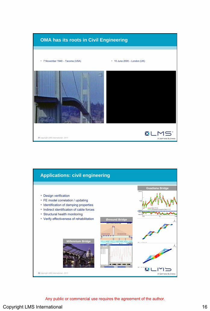
In-flight OMA mode shape (4/4)
30 copyright LMS International - 2011
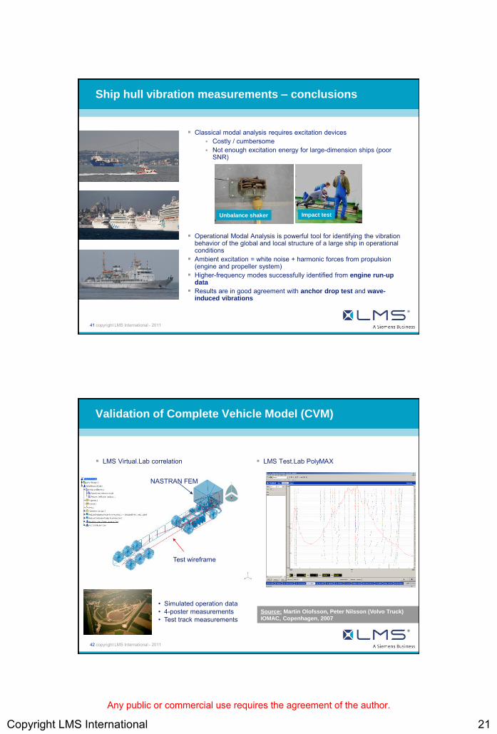
Conclusions
In-flight testing
OMA: some important flutter-critical modes not excited EMA: some modes mainly excited by the turbulences
may not be identified Conclusion: beneficial to use artificial excitation, but
data analysed with stochastic methods that also take into account the unknown excitation
Airbus flight test team evaluated LMS Test.Lab using large-aircraft data
―We actually achieved better results using operational techniques than with classical EMA. We found more modes. The synthesis was better with higher correlation and fewer errors. And the in-flight mode shapes looked much nicer!‖
―We found that the exponential window, which allowed for cross-correlation calculations was a good de-noising tool for our in-flight data.‖
True Air Speed(knots)
Altitude (feet)
40,000
30,000
20,000
10,000
100 200 300 400 500
MACH 0.95
MACH 0.90
MACH 0.85
True Air Speed(knots)
Altitude (feet)
40,000
30,000
20,000
10,000
100 200 300 400 500
MACH 0.95
MACH 0.90
MACH 0.85
Any public or commercial use requires the agreement of the author.
Copyright LMS International 16
31 copyright LMS International - 2011
OMA has its roots in Civil Engineering
7 November 1940 – Tacoma (USA) 10 June 2000 – London (UK)
32 copyright LMS International - 2011
Applications: civil engineering
Design verification FE model correlation / updating Identification of damping properties Indirect identification of cable forces Structural health monitoring Verify effectiveness of rehabilitation
0.30 3.00 LinearHz
-130.00
-100.00
dBg2
Deck:117:+ZSynthesized Crosspow er Deck:117:+Z
0.30 3.00 LinearHz
0.30 3.00 Hz-180.00
180.00
°
Guadiana Bridge
Millennium Bridge
Øresund Bridge
Any public or commercial use requires the agreement of the author.

Copyright LMS International 17
33 copyright LMS International - 2011
23/11/2002: Bradford City – Sheffield United: 0 – 5
Data acquisition: 4 h Sampled at 80 Hz (down-sampled to 20 Hz) Sliding RMS value ( — )
1000 samples, 50% overlap
0.00 15000.00 s-0.02
0.02 R
eal
(m/s
2 )
-0.20
0.20
Rea
l
(m/s
2 )
F time_record roof:1:+X / Root Mean SquareB time_record roof:1:+X
Goal 1 Goal 2 Goal 3 Goal 4 Goal 5
Half time Empty Filling Seated Emptying
End of game
34 copyright LMS International - 2011
Continuous monitoring of the
Bradford and Bingley Stadium
Data: Paul Reynolds, Sheffield University
Any public or commercial use requires the agreement of the author.

Copyright LMS International 18
35 copyright LMS International - 2011
Ambient Vibration Testing of the Millau Viaduct
36 copyright LMS International - 2011
Millau Viaduct – LMS Test.Lab PolyMAX results
Source: E. Caetano,
F. Magalhaes, A.
Cunha (univ. Porto),
O. Flamand, G.
Grillaud (CSTB)
EVACES Conference,
Porto, 2007
Any public or commercial use requires the agreement of the author.

Copyright LMS International 19
37 copyright LMS International - 2011
Guadiana Bridge – Modal parameters
Mode Freq.
[Hz]
Damp.
[%]
1 0.384 1.32
2 0.522 1.20
3 0.558 1.57
4 0.951 0.69
5 1.036 0.49
6 1.299 0.46
Mode Freq.
[Hz]
Damp.
[%]
7 1.448 0.54
8 1.654 0.66
9 1.880 0.57
10 2.248 0.60
11 2.547 0.72
12 2.778 0.23
PolyMAX – single analysis results
38 copyright LMS International - 2011
Ship hull vibration measurements
5 Three-axis acceleration sensors At forward, aft ends and center of upper deck At end of front & aft of compass deck (longitudinal,
lateral and torsion vibrations measurement of deckhouse)
7 Mono-axis acceleration sensors (vertical direction)
On the right side of upper deck
前後、左右、上下方向
11 12
Data Measurement
Test.Lab & SCADAS-Mobile
Long., trans. and vert. direction
Vertical direction
Upper deck
Compass deck
Master/Slave configuration
Any public or commercial use requires the agreement of the author.

Copyright LMS International 20
39 copyright LMS International - 2011
Change of Vibration Acceleration at aftbody
Change of order components for engine speed
Change of frequency component for
engine speed
0 50Hz
DeckL:1:+Z (CH3)
380
680
rpm
Rp
m E
xtr
(T
1)
-140.00
-40.00
dB g
1.00 2.00
6.00
380 680rpm
0.00
7.40e-3
g
545.00 665.00
F Order 1.00 DeckL:1:+ZF Order 2.00 DeckL:1:+ZF Order 6.00 DeckL:1:+Z
0 50Hz
DeckL:1:+Z (CH3)
380
680
rpm
Rp
m E
xtr
(T
1)
-140.00
-40.00
dB g
0.37 1.00 1.49
3.40 9.1011.10
14.20
380 680rpm
0.00
7.40e-3
g
545.00 665.00
F Frequency 3.40 Hz DeckL:1:+ZF Frequency 9.10 Hz DeckL:1:+ZF Frequency 11.10 Hz DeckL:1:+ZF Frequency 14.20 Hz DeckL:1:+Z
Measurement point 1, Z direction
40 copyright LMS International - 2011
OMA results: hull vertical vibration modes
Hull Vertical
3 nodes 6.1 Hz
Hull Vertical
4 nodes 9.1 Hz
Hull Vertical
5 nodes 11.1 Hz
Hull Vertical
6 nodes 14.3 Hz
0
5
10
15
20
25
30
0 5 10 15 20 25
Mode number
Fre
qu
en
cy [
Hz]
Glabal vibration mode Hull lateral mode
Hull vertical mode Upper structure mode
Hull Vertical
2 nodes 3.4 Hz
Any public or commercial use requires the agreement of the author.
Copyright LMS International 21
41 copyright LMS International - 2011
Ship hull vibration measurements – conclusions
Classical modal analysis requires excitation devices Costly / cumbersome Not enough excitation energy for large-dimension ships (poor
SNR)
Operational Modal Analysis is powerful tool for identifying the vibration behavior of the global and local structure of a large ship in operational conditions
Ambient excitation = white noise + harmonic forces from propulsion (engine and propeller system)
Higher-frequency modes successfully identified from engine run-up data
Results are in good agreement with anchor drop test and wave-induced vibrations
Unbalance shaker Impact test
42 copyright LMS International - 2011
Validation of Complete Vehicle Model (CVM)
LMS Virtual.Lab correlation LMS Test.Lab PolyMAX
Test wireframe
NASTRAN FEM
Source: Martin Olofsson, Peter Nilsson (Volvo Truck)
IOMAC, Copenhagen, 2007
• Simulated operation data • 4-poster measurements • Test track measurements
Any public or commercial use requires the agreement of the author.

Copyright LMS International 22
43 copyright LMS International - 2011
Mode shape correlation (MAC)
OMA shows better correlation with FEM than ODS
Not all FEM modes could be found in operational data (not well excited by 4-poster, too highly damped)
Others have high correlation
ODS
ODS / OMA vs. FEM
FEM
Reduced FEM vs. OMA mode shape
OMA
44 copyright LMS International - 2011
Testing and identification of active systems
Intelligent and complex systems engineering Multi-physics system simulation: 1D,
3D, control State estimator: processing data by
models • Applied to Vehicle Dynamics
Control (Flanders’ Drive project) Testing of active system
Model validation and updating Case study
Ford S-MAX 4-poster and Proving Ground tests
Steering
Suspension force
elements
Suspension force
elements
15 DOF
Compliances
Sensors
Tires
Road input / 4 Post Shaker
Steering
Suspension force
elements
Suspension force
elements
15 DOF
Compliances
Sensors
Tires
Road input / 4 Post Shaker
Steering
Suspension force
elements
Suspension force
elements
15 DOF
Compliances
Sensors
Tires
Road input / 4 Post Shaker
Steering
Suspension force
elements
Suspension force
elements
15 DOF
Compliances
Sensors
Tires
Road input / 4 Post Shaker
Any public or commercial use requires the agreement of the author.

Copyright LMS International 23
45 copyright LMS International - 2011
Full-scale modal wind turbine tests: comparing shaker excitation
with wind excitation
© NREL: U.S. Wind Resource (50m)
46 copyright LMS International - 2011
EMA – Mode shapes (avi)
Tower fore-aft Tower side-to-side 1st rotor symmetric flap
Any public or commercial use requires the agreement of the author.

Copyright LMS International 24
47 copyright LMS International - 2011
Shaker excitation (EMA) vs. wind excitation (OMA)
Excellent agreement between EMA & OMA Modes not well excited by wind not identified by OMA
48 copyright LMS International - 2011
Conclusions
Operational Modal Analysis is a mature technology
High-quality data acquisition Advanced parameter estimation algorithms Commercial software implementations Industrial applications
Last decade, evolution in
Technology Usability Applicability: no isolated results but part of
engineering workflow
• Civil engineering • Aerospace engineering • Automotive engineering
Any public or commercial use requires the agreement of the author.

Copyright LMS International 25
Marie Curie Graduate School on Vehicle Mechatronics & Dynamics, Leuven, 5-8 February 2013 Bart Peeters
Thank you
Related technical papers can be downloaded from
www.lmsintl.com
Any public or commercial use requires the agreement of the author.