Deliverable D 1.3

Nutrient Balances for Case Study Regions Austria and Hungary

and

Deliverable D 1.4 Comparison of results from case study investigations and evaluation of key factors influencing the nutrient fluxes

Vienna, September 2004

1

Authors:

Matthias Zessner Christian Schilling Oliver Gabriel Galina Dimova Christoph Lampert

Adam Kovacs Adrienne Clement Kalman Buzas

Carmen Postolache

Department of Sanitary and Environmental Engineering Budapest University of Technology

Department of Systems Ecology and Sustainable Development University of Bucharest

Institute for Water Quality and Waste Management Vienna University of Technology

2

Part I Nutrient Balances for Austrian case study regions Pages 1 - 131

Part II Nutrient Balances for Hungarian case study regions Pages 1 - 75

Part III Comparison of results from case study investigations and evaluation of key factors influencing the nutrient fluxes Pages 1 – 51

3

VIENNA UNIVERSITY OF TECHNOLOGY INSTITUTE FOR WATER QUALITY

AND WASTE MANAGEMENT

Part I

DELIVERABLE D 1.3

NUTRIENT BALANCES FOR CASE STUDY REGIONS

AUSTRIA

4

Table of Content 1. INTRODUCTION................................................................................................. 5

2. METHODOLOGY................................................................................................ 5

3. DESCRIPTION OF DATA................................................................................... 6

4. CHARACTERISATION OF THE CASE STUDY REGIONS................................ 9

4.1. General characterisation 9

4.2. Population and waste water disposal 20

4.3. Agricultural production 22

4.4. Groundwater characterisation 25

5. DATA ANALYSES............................................................................................ 28

5.1. Surface water data 28

5.2. Groundwater data 43

5.3. Groundwater-Surface water-Interactions 53

5.4. Groundwater residence time and its influence on nitrogen discharges 68

5.5. Nutrient surplus and content in agriculture soils 80

6. MONERIS APPLICATION ................................................................................ 89

6.1. Methodological aspects 89

6.2. Results 89

7. SWAT APPLICATION....................................................................................... 92

7.1. Methodology 93

7.2. Results 95

7.3. Conclusions 99

8. MATERIALS ACCOUNTING CALCULATIONS ............................................... 99

8.1. Methodology 99

8.2. Results of Materials accounting calculations 100

9. COMPARISON OF RESULTS WITH DIFFERENT APPROACHES............... 117

9.1. Groundwater and soil concentrations 117

9.2. River loads and retention in surface and groundwater 120

9.3. Sensitivity analyses 123

9.4. Conclusions from Austrian case study investigations 126

10. LITERATURE .............................................................................................. 127

5

1. Introduction The relations between human activities (emissions) and concentrations and/or transported loads and/or effects in receiving water systems have to be studied in order to derive effective measures of water protection. The knowledge about relevant processes of transformation, retention and transport of nutrients and their quantification is fragmentary. Existing approaches for quantification often use assumptions and empirical equations, which were derived for special conditions and cannot simply be transferred to other regions. The goal of workpackage 1 of the daNUbs project is to improve the understanding of nutrient turnover in a region and of the relation of emissions and in-stream loads of nutrients (transport, retention, denitrification). This report contains deliverable D1.3 (Report on nutrient balances for case study regions) and deliverable D1.4 (Comparison of results from investigations in case study investigations and evaluation of key factors influencing nutrient fluxes in a region) of workpackage 1. The goal was to perform comprehensive nutrient (N, P) balances of 6 case study regions with different climatic and hydrologic conditions. This report contains results from 5 case study areas: The Ybbs and the Wulka river in Austria (these results are presented in Part I of this Report), the Lonjai and the Zala river in Hungary (these results are presented in Part II of this report) and the Neajlov river in Romania (these results are partly included into the comparison between catchments in deliverable D1.4 which is Part III of this report. The detailed presentation of results from the Romanian case study are not ready yet and will be presented in a seperat report). Results from the Bulgarian case study region (Lesnovska river) have not been included into this report because of the big delay of this work. A comparison of the different catchments and an integrated conclusions is presented in the Deliverable D1.4 (evaluation of key factors influencing nutrient fluxes of a region), which constitutes Part III to this report. In addition to the task to increase the understanding on processes which are relevant for nutrient balances on catchment level, the calculations in case study areas have been used as test regions for the methodologies applied for the whole Danube basin. In this report mainly the MONERIS emission model is tested. Test runs for the Danube Water Quality Model are presented in deliverable D5.10 (DWQM simulations for case studies). In order to fulfil the tasks of this report, several approaches in the different case study regions have been used and will be specified in the following sections. The report is structured in a way that following this introduction the results of nutrient balance calculations with different approaches will be presented for the case study regions of each country seperatly.

2. Methodology The approaches which were used for the quantification of nutrient fluxes in the Austrian case study regions are presented in this chapter of the report. The report starts with a characterisation of the regions in respect to important parameters for nutrient balances. In the following the calculations with different approaches are explained and results are shown. At the end the comparison of results with different approaches is presented.

6

Evaluation of data from surface waters and groundwater on catchment level were used to derive nutrient loads and to estimate the retention (sedimentation and denitrification). More detailed data, as they are available on catchment scale, of river water, multilevel wells (situated in the river sediment) and groundwater wells (located in the groundwater flow close to the river system) were used at two cross sections (one at the Wulka and one at the Ybbs) to evaluate the retention (denitrification) in the groundwater flow and in the boundary layer between surface water and groundwater. For sections of the catchment areas where information on the groundwater table was available, a method was developed to calculate the regional distributions of groundwater flow times from a certain point of the catchment to the surface waters (residence time). This spatial information was used to calculate nitrogen retention (by denitrification) in the groundwater and a distribution of the contribution of areas to the total nitrogen emissions to the surface waters via groundwater. All relevant emission pathways of nutrients to surface waters are reflected in the MONERIS emission model. This model was applied for a number of subcatchments in the Wulka and Ybbs catchment. The information required by the MONERIS approach in order to calculate the nutrient emissions into the groundwater and surface waters is not always sufficient to derive front-end-measures. Especially information on material flows and emissions from private households, forestry, industry and agriculture are not included in detail or should be refined. Therefore, further investigations to complete the data base obtained for the MONERIS application and to increase the number of possible measures to reduce nutrient emissions to surface waters were performed based on the method of materials accounting. Already in deliverable D1.1 (water balance calculations for case study regions) the SWAT model was applied for water balance calculations. In this report it was tried to use the SWAT model for nutrient balance calculations as well. Finally calculations with different approaches were compared to each other and measurements and the sensitivity of several calculations were checked based on a variation of assumptions.

3. Description of data A description of the data, which were used for the calculation of the water balances for the case study regions were already presented in deliverable D 1.1. A summary of data that were acquired for the water and nutrient balance calculations can be found in deliverable D 1.2. Table 3-1 gives a summary information about all data that were obtained and used for the nutrient balance calculations in the Wulka and the Ybbs catchment. The table gives an overview about the availability of the data, the data format, the data source, the time span covered by the data or the last update as well as the spatial resolution.

7

Table 3-1: Summary of format, source, time span and resolution of the available data

Maps availability format Source time span Resolution river net yes digital maps 1, 2 actual 1:50000 catchment boundaries yes digital maps 1, 2 actual 1:50000 administrative boundaries yes digital maps 1, 2 actual 1:50000 Digital elevation model (DEM) yes digital maps 1, 2 actual 25m grid topographic map yes digital maps 1 actual 1:50000 land use map yes digital maps 5 actual 30m grid geological maps yes digital maps 1, 3 actual 1:50000 soil types (soil map) yes digital maps 5 actual 1:25000 drained areas Wulka partly analog maps 2 Different eroded areas (soil loss map) no Location of monitoring stations yes digital/analog 5 actual location of municipal and industrial discharges digital/analog 1, 2 actual

Statistical data availability format Source time span Resolution crop statistics (area, yield) yes digital data 4 1960 - municipality fodder production yes digital data 4 1960 - county fodder consumption no estimates Livestock No. or animal units yes digital data 4 1960 - municipality

mineral fertilizer application yes/no own estimates

and analog data till 1995

1960- county/federal state

food production (meat, milk, eggs and non-animal food) yes digital data 1960 - county

population yes digital data 4 1960 - Municipality /settlement

food consumption yes 4 1960- country use of detergents (washing powder, dish washing etc.) yes country

spec. P and N emissions to sewer systems (based on population or population equivalent)

no estimates

application of sewage sludge yes estimates 5 1990- municipality application of compost no Waste water statistics

Pop. connected to sewer system yes analog/digital data 1, 2 1971- municipality

Pop. connected to WWTP´s yes analog data 1, 2 actual municipality Portion of combined sewers no estimates

Portion of separate sewers no estimates

population connected to septic tanks and pits yes analog data 1, 2 1971- municipality

information on the fate of content from septic tanks and pits no

8

Inventory of point discharges (municipal/industrial)

Location yes analog 1, 2 actual capacity of WWTP yes analog data 1, 2 actual

actual loading yes digital data 5, 2 actual two to five days a week

population connected yes analog data 1, 2 actual Treatment stages yes analog data 1, 2 actual inflow and effluent loads (discharge Q, N, P, org. carbon) yes digital data 5, 2 actual two to five days a

week In addition for big and direct discharging industries:

information on the production process not relevant

Treatment of manure, removal efficiency of these treatment plants, emission data

not relevant

Monitoring data

river discharges yes digital data 1, 2 1977- 5 stations, hourly, daily

Groundwater level yes digital data 1, 2 1970- Several stations, weekly

water level (surface water) yes digital data 2 1976- 5 stations, daily Water temperature (surface water) yes digital data 2 1991- 1 station, daily

precipitation yes digital data 1, 2 1971- 16 stations, hourly

temperature air yes digital data 1, 2 1990- 16 stations, Tmax, Tmin

relative humidity yes digital data 2,7 1970- 24 stations, daily wind velocity yes digital data 2 1990- 4 stations, daily hours of sunshine yes digital data 7 1970- 20 stations, daily solar radiation yes digital data 2,7 1970- 24 stations, daily potential ET yes digital data 7 1970- 20 stations, daily snow height yes digital data 1,2 1970- 15 stations, daily

Conc. of substances in rivers yes digital data 1, 2 1991- 1 station daily, 4 stations monthly, 1)

Conc. of substances in rivers 6 Conc. of N and P in drainage water no

Conc. of substances in groundwater yes digital data 1, 2 1991- 17 stations, three

monthly Conc. of substances in groundwater 6

Conc. of N, P and silica in topsoil yes analog data 4km grid N deposition yes analog data 1986 some measurementsP deposition no N+P+silica content in detergents: cleaning processes (washing powder, dish washing)

yes actual Country

N-Emissions by traffic, energy supply, room heating etc. yes 1980 Country

Further: Location of hydro power plants yes

location/ discharge of springs yes analog data 2 1995- 4 stations, monthly

9

Sources: 1. Amt der Niederösterreichischen Landesregierung (Agency of the federal government of Lower

Austria) 2. Amt der Burgenländischen Landesregierung (Agency of the federal government of

Burgenland) 3. Geologische Bundesanstalt (Geological federal agency) 4. Österreichisches Statistisches Zentralamt (Statistik Austria) 5. developed within the daNUbs-project 6. own measurements 7. ZentralAnstalt für Meteorolgie und Geodynamik (Central Institute of meteorology and

geodynamics)

4. Characterisation of the case study regions

4.1. General characterisation Austria covers an area of about 83.870,9 km2 and is a little bit smaller then Hungary and a little bit bigger than the Čzech Republic (Statistik Austria). With about 8 million inhabitants the population density is 95 inh/km2. The two case study regions are located in two different federal states (Figure 4-1). The Ybbs catchment is located in the West of the federal state of “Lower Austria” and has 29 municipalities within the catchment area of about 1105 km2. The Wulka catchment is located in the North-East of the federal state “Burgenland” and within its catchment area of about 383 km2 41 municipalities are located.

Figure 4-1: Location of the case study regions (with subcatchments) in Austria within the administrative structure of Austria

A first characterisation of the two Austrian case study catchments in terms of the elevation, landuse, soil and geological characteristics was already given in Deliverable D 1.1. In this report most important information is repeated and additional information for characterisation

10

of the regions, mainly in respect to population, waste water management and agriculture is given. Table 4-1 shows a summary of the main characterisation of the Wulka and Ybbs catchment with the considered subcatchments. For nutrient balance calculations the Ybbs catchment was subdivided into three subcatchments: the upstream catchment till the measuring point Opponitz at the Ybbs (later on named “Opponitz”; the subcatchment of the Url upstream of Krenstetten (called “Krenstetten”) and the subcatchment downstream of Opponitz and Krenstetten, upstream of the measuring point Greimpersdorf (later on called “Greimpersdorf net”). The total catchment is called “Ybbs total” or “Greimpersdorf total”. The Wulka catchment is subdivided into five subcatchments. The most upstream is “Walbersdorf” it is the catchment down to the measuring station in Walbersdorf at the Wulka. “Wulkaprodersdorf net” is the catchment down to the measuring point Wulkaprodersdorf excluding the subcatchment Walbersdorf, while “Wulkaprodersdorf total” is this subcatchment including “Walbersdorf”. The subcatchments “Nodbach” and “Eisbach” are the catchments of these creeks down to the sampling points at these creeks in St. Margarethen and Oslip, respectively. “Schützen net” is the subcatchment upstream of the station Schützen at the Wulka. Again in “Schützen net the upstream subcatchments are not included whereas in “Schützen total” or “Wulka total” the whole catchment is considered. For some considerations the measuring point at the Wulka in Trausdorf and the related subcatchment are considered as well.

11

Table 4-1: Main characteristics of case study regions, subdivided in into sub-catchments (suggested as format for all sub-catchments)

CountryName of the river

subcatchment total Opponitz Url/ Krenstetten

Greimpersdorf net total Walbersdorf Wulkaproders

dorf net Nodbach Eisbach Schützen net

Total catchment area km2 1105 506 151 448 383 76 142 47 64 55Share of arable land % 12 0 37 17 54 31 62 64 50 62Share of agricultural grassland % 27 12 41 40 12 13 12 14 10 10Share of forests % 52 75 20 38 28 50 21 16 29 22Share of consolitated rock % 65 79 54 53 56++ 26 82 37 68 34

main geological unitdolomite/

flyschdolomite/ limestone

sandstone/ flysch

sediments /dolomite

marl/ sediments - marl sediments

marl/ sediments sediments

main soiltypes rendzina rendzina luvisolrendzina/

luvisolchernosem/

luvisol luvisol chernosem chernosem chernosem chernosemN-fertiliser application* kg/haAA/a 150 100 178 152 100 110 117 90 81 73

P-fertiliser application* kg/haAA/a 43 31 47 44 26 36 32 24 21 20

N-surplus in agriculture kg/haAA/a 73 24 88 74 50 43 55 47 55 48

P-surplus in agriculture kg/haAA/a 25 15 28 29 17 14 20 14 15 12

N-in agricultural soil g/kg 3.6 5.9 2.6 3.5 1.5P in agricultural soil g/kg 0.8 0.6 0.8 0.8 0.7 0.7 0.8 0.6 0.6 0.6N-deposition kg/ha/a 19 16 24 20 13.5 13.5 13.5 13.5 13.5 13.5average N-surplus on total area kg/ha/a 40 17 74 51 38 26 44 40 38 38average P-surplus on total area kg/ha/a 10 2 22 17 11 6 15 11 9 9mean slope % 30 43 14 32 8 15 10 5 7 8average precipitation mm/a 1390 1680 1029 1185 665 711 663 636 653 630average runoff** mm/a 868 1170 434 673 49 91 47 54 35 9share of groundwater flow % 71 70 67 73 58 78 75 74 25share of direct flow % 28 30 31 25 16 18 21 26 21share of point source contribution % 0.7 0.1 2.4 1.7 26 4 4 0 54

population density inh/km2 68 17 81 122 133 153 101 147 208 89Share conneceted to sewerage % 74 83 63 75 95 87 100 100 94 100Share conneceted to wwtp % 74 83 63 75 95 87 100 100 94 100predominant waste water treatment C, N(D), P C, N, D, P C, N, P C, N, (D), (P) C, N, D, P C,N, (D), P no discharge no discharge C, N, D, P C, N, D, PIndustrial activity medium no low medium low low low low low lowarea specific river loads N kg/ha/a 19 15 23 21 5 5 4 4 6 8area specific river loads P kg/ha/a 0.8 0.3 0.6 1.3 0.3 0.3 0.1 0.1 0.3 0.8

* total application of fertilzer (incl. Manure, or sewage sludge) related to agricultural area (haAA)in use (grassland and arable land)**without contribution from point sources

AustriaYbbs Wulka

12

4.1.1. The Ybbs catchment Figure 4-2 shows the elevation distribution of the Ybbs catchment with the location of the groundwater, surface water level and quality measurement stations. Due to the hydrogeological conditions (see D 1.1) nearly almost of the groundwater measurement points are located in the north of the catchment. This is the only part of the catchment where porous aquifers are located. The more moving to the south of the catchment the more bedrock aquifers and aquicludes become dominant. The elevation distribution in the Ybbs catchment ranges from 250m to 1900m above sea level with an average slope of 32%. The subbasin Opponitz represents the more mountainous part of the watershed with an average slope of 45% (elevation from 390 to 1900m), whereas the subbasin Krenstetten has a relatively small elevation range (300-900m) and an average slope of 14%. In coincidence with the elevation and slope characteristics there is a significant increase in precipitation from the northern part of the watershed (Krenstetten, Greimpersdorf) to the south (Opponitz).

Figure 4-2: Elevation characteristics and overview on the location of the groundwater and surface water measurement stations for the Ybbs catchment

Water balance characteristics The Ybbs catchment is situated in the northern pre-alpine region of Austria, where due to the typical north-west winds north congestion-weather conditions have a relatively frequent occurrence. Thus, the Ybbs catchment has a high amount of average annual precipitation between 550 in the north and more than 1800 mm in the south of the catchment. A detailed

13

water balance was already presented in D1.1. With the extension of the calculation period the following water balance was calculated using the SWAT 2000 model: Table 4-2: Water balance components of the Ybbs catchment, calculated for the period 1992-2000 (without storage changes and transmission losses from river)

[mm/a] [%] Remarks Average annual precipitation 1357 Evapotranspiration 375 28 [%] related to precipitation River discharge 905 67 [%] related to precipitation Surface runoff 238 26 [%] related to river discharge Lateral runoff 369 40 [%] related to river discharge Baseflow 305 33 [%] related to river discharge Point source contribution 7 1 [%] related to river discharge Tile drainage runoff 0 0 [%] related to river discharge Snow fall 191 14 [%] related to precipitation Snow melt 145 11 [%] related to precipitation Due to changes in some parameter definitions the proportion of the runoff components baseflow, lateral flow and surface runoff differ from those already presented in D 1.1. About 2/3 of the average annual precipitation leaves the catchment as runoff. The highest contribution to the total runoff is by lateral flow (40%) followed by the base flow (33%), which together form the groundwater flow (see deliverable D1.1). With 25% the contribution of the surface runoff to the total runoff is quite high. The high contribution of the lateral flow can be explained by the small share of unconsolidated aquifers in the part downstream of the catchment. The most part of the catchment, especially the part upstream the confluence of the rivers Ybbs and Kleine Ybbs is dominated by aquifers consisting of consolidated rocks. The regional variation of the water balance is shown in Table 4-3. Differences occur mainly in the amount of runoff and in the share of the runoff components. Evapotranspiration is very similar in all three subcatchments. Table 4-3: Regional distribution of the most important water balance components for the period 1992-2000 (without storage changes and transmission losses from river)

Greimpersdorf total

Krenstetten Opponitz

[mm/a] [%] [mm/a] [%] [mm/a] [%] Average annual precipitation 1357 - 972 - 1657 - Evapotranspiration 375 28 383 39 370 22 River discharge 905 67 525 54 1212 73 Surface runoff 238 26 107 20 315 26 Lateral runoff 369 40 245 47 520 43 Baseflow 305 33 173 33 377 31 Snow fall 191 14 104 11 266 16 Snow melt 145 11 64 7 213 13 In the most upstream subbasin Opponitz 43% of total runoff is lateral flow. The relative contribution of the surface runoff (26%) is as high as at the main watershed outlet Greimpersdorf, and the amount of baseflow (31%) is nearly equal to the surface runoff. The

14

high contribution of the lateral flow is explainable by the small share of unconsolidated aquifers in this part of the catchment. In the subbasin Krenstetten the distribution of the runoff components is nearly of the same kind. The contribution of the lateral flow (47%) to the total runoff is still the highest, followed by the baseflow (33%). The share of surface runoff is only a little lower than in the other subbasins. Due to the distinctive lower amount of precipitation the total runoff from the subbasin is only half of the total runoff of the Ybbs catchment. But in regard to the main watershed outlet Greimpersdorf the subbasin Krenstetten compensates the smaller contribution of the surface runoff with a little higher contribution of the lateral flow.

Figure 4-3: Annual variation of the precipitation, evapotranspiration and the river discharge with the distribution of the discharge components for the subbasins Opponitz, Krenstetten and Greimpersdorf

As shown in Table 4-3, the average annual amount of precipitation varies between the subbasins. Additionally, there is also a variability in the annual amount of precipitation within the years (see Figure 4-3) e.g. in the subbasin Opponitz between 1400 and 2000 mm/a. The evapotranspiration does not show big differences over the years. For the subbasin Krenstetten the annual amount of precipitation is smaller, the annual amount ranges between 800 and

Opponitz

0

400

800

1200

1600

2000

1991

1992

1993

1994

1995

1996

1997

1998

1999

2000

2001

annu

al a

mou

nt [m

m/a

]

precipitationevapotranspirationdischarge

Opponitz

0%

20%

40%

60%

80%

100%

19911992

19931994

19951996

19971998

19992000

2001

rela

tive

cont

ribut

ion

[%]

groundwaterlateral flowsurface runoff

Krenstetten

0

400

800

1200

1600

2000

1991

1992

1993

1994

1995

1996

1997

1998

1999

2000

2001

annu

al a

mou

nt [m

m/a

]

precipitationevapotranspirationdischarge

Krenstetten

0%

20%

40%

60%

80%

100%

19911992

19931994

19951996

19971998

19992000

2001

rela

tive

cont

ribut

ion

[%]

groundwaterlateral flowsurface runoff

Greimpersdorf

0

400

800

1200

1600

2000

1991

199219

93199

419

951996

1997

199819

99200

020

01

annu

al a

mou

nt [m

m/a

]

precipitationevapotranspirationdischarge

Greimpersdorf

0%

20%

40%

60%

80%

100%

1991

1992

1993

1994199

5199

619

9719

981999

2000

2001

rela

tive

cont

ribut

ion

[%]

groundwaterlateral runoffsurface runoff

15

1200 mm/a. The annual discharge in the subbasin Krenstetten is nearly equal to the annual amount of evapotranspiration. For the watershed outlet Greimpersdorf the annual behaviour is a mixture of those of the subbasins Opponitz, Krenstetten and Greimpersdorf. The annual amount of precipitation ranges between 1200 and 1600 mm/a. The discharge corresponds in its variability more to the precipitation than to the evaporation. In the seasonal variation of the relative contribution of the runoff components (see Figure 4-3) only small differences in the runoff components distributions between the subbasins occur. The contribution of the different runoff components does not significantly depend on the annual amount of precipitation. The contribution of the surface runoff doesn’t correspond to the annual amount of precipitation. Its more dependent on the intra-annual precipitation characteristics of the subbasin, like the occurrence of storm events. The lateral flow is of nearly consistent amount so that the baseflow characteristics results mainly from those of the surface runoff and the lateral flow. Characterisation of the Geology The geological formations of the Ybbs watershed can be divided into two main parts consisting of consolidated rocks (covering 2/3 of the watershed area) and unconsolidated gravels and sediments (covering 1/3 of the watershed area). The unconsolidated sediments constitutes mainly of terrace gravels and alluvial deposits. They can be found in the northern part of the watershed (subbasin Krenstetten, around Greimpersdorf) and they form the aquifers partly covered by loam. The consolidated rocks mainly consist of limestone, dolomite, flysch and sandstone and can be found mainly in the southern, more upstream part of the watershed of the subbasin Opponitz. There are only local, river conducted aquifers. Soil characteristics The soils in the Ybbs watershed can be characterised mainly as silty soils. The 18 soil types of the Ybbs watershed have of an average content of 17% sand /61% silt /22% clay.

4.1.2. The Wulka catchment Figure 4-4 shows the elevation distribution of the Wulka catchment with the location of the groundwater and surface water level and quality measurement stations. Due to the hydrogeological formations most of the groundwater quality and groundwater level measurement stations are located downstream the gauging stations Walbersdorf (Wulka river) and Wulkaprodersdorf (Wulka river). Especially nearby the gauging station Schützen the density of groundwater measurement points is higher than in other parts of the catchment. Thus, this region was used for more detailed analyses of the groundwater table, the groundwater flow direction and residence time and the behaviour of conservative and non-conservative substances in the groundwater. The elevations in the Wulka catchment range from 125m to 750m above sea level and do characterise the catchment as relatively flat region with an average slope of 8% (Figure 4-4). The most elevated subbasin is Walbersdorf with an average subbasin slope of 15%, followed by Wulkaprodersdorf with 10% average slope (164m-742m), Eisbach with 6,5% average slope (131m-463m) and the Nodbach with 4% average slope (126m-367m).

16

Figure 4-4: Elevation characteristics and overview on the location of the groundwater and surface water measurement stations for the Wulka catchment

Soil characteristics

Figure 4-5: Soil distribution in the Wulka catchment

17

In addition to D1.1 a more detailed soil map (Figure 4-5) could be obtained and was introduced to the calculations using the SWAT 2000 model. With exception of the soil types which covered by forest (together 27,9%), the dominating soil types are the black soils (chernosem 26,4%; humid black soil 12,6%) followed by the brown soils covering mainly casual sediments. Of importance are also the settlements. They cover a percentage of 6,9% of the soils in the catchment. All the other soil types have a share smaller than 3% of the total catchment area.

settlement6.9%

alluvial soil2.6%

tchernosem26.4%

forest27.9%

rawish soil2.1%

others4.0%

kolluvium1.6%

humid black soil 12.6%

rawish cultivated soil

2.5%

rock brown soil 1.5%

casual sediment

brown soil11.9%

Figure 4-6: Fraction of the catchment area covered by each soil type

Water balance characteristics The Wulka catchment is situated in the eastern part of Austria, where a much smaller amount of precipitation is available for runoff generation compared to the Ybbs catchment. With an average annual precipitation amount ranging from 670 to 760mm there is only half of the precipitation available in relation to the Ybbs catchment. A detailed water balance was already calculated in D1.1. Due to changes in some of the model definitions of the SWAT 2000 model the main water balance characteristics are presented here again. The following water balance was calculated using the SWAT 2000 model: Table 4-4: Water balance components of the Wulka catchment, calculated for the period 1992-1999 (without storage changes and transmission losses from river)

[mm/a] [%] Remarks Average annual precipitation 685 Evapotranspiration 525 77 [%] related to precipitation River discharge 101 15 [%] related to precipitation Surface runoff 7 7 [%] related to river discharge Lateral runoff 12 12 [%] related to river discharge Baseflow 43 42 [%] related to river discharge Point source contribution 28 28 [%] related to river discharge Tile drainage runoff 11 11 [%] related to river discharge Snow fall 40 6 [%] related to precipitation Snow melt 37 5 [%] related to precipitation The share of precipitation contribution to the runoff is only 15%. Most of the precipitation (77%) is going to evapotranspiration. The highest contribution to the total runoff is by base flow (42%), followed by point sources (28%). This underlines the importance of the discharges coming from the wwtp’s in the catchment. A lot of cultivated areas are drained.

18

Thus, the contribution by runoff from drained areas (11%) has to be considered as well although the implementation of drained areas into the SWAT 2000 model is not well defined yet. Lateral flow contributes 12% to the total runoff. The regional variation of the water balance is shown in Table 4-5. Differences occur mainly in the amount of precipitation and in the share of the runoff components. Table 4-5: Regional distribution of the most important water balance components for the period 1992-1999 (without storage changes and transmission losses from rivers)

Walbersdorf Wulkaprodersdorf total

Schützen total

[mm/a] [%] [mm/a] [%] [mm/a] [%] Average annual precipitation 793 733 685 - Evapotranspiration 555 70 530 72 525 77 River discharge 110 14 83 13 101 15 Surface runoff 7 6 9 11 7 7 Lateral runoff 38 35 19 23 12 12 Baseflow 65 59 55 66 43 42 Snow fall 46 6 42 6 40 6 Snow melt 39 5 36 5 37 5 As the precipitation the evapotranspiration increases a little from the main watershed outlet Schützen to the most upstream subbasin Walbersdorf. The most important difference is that the two subbasins Walbersdorf and Wulkaprodersdorf do not contain significant discharges from wwtps. In the subbasin Schützen, the contribution from wwtp’s is part of the total runoff which results in a decrease of the relative contribution of the other runoff components. In the upstream subbasins Walbersdorf and Wulkaprodersdorf the base flow contributes around 60% to the total runoff. The amount of lateral flow decreases from the subbasin Walbersdorf to the main watershed outlet Schützen. Together with baseflow the groundwater discharge (baseflow and lateral flow) is 94 % in Walbersdorf, 89 % in Wulkaprodersdorf and 54 % in Schützen.

Figure 4-7: Annual variation of the precipitation, evapotranspiration and the river discharge with the distribution of the discharge components for the subbasin Walbersdorf

Walbersdorf

0

400

800

1200

1992 1993 1994 1995 1996 1997 1998 1999

annu

al a

mou

nt [m

m/a

]

precipitationevapotranspirationriver discharge

Walbersdorf

0%

20%

40%

60%

80%

100%

1992 1993 1994 1995 1996 1997 1998 1999

rela

tive

cont

ribut

ion

[%]

Tile Drainagegroundwaterlateral flowsurface runoff

19

Figure 4-8: Annual variation of the precipitation, evapotranspiration and the river discharge with the distribution of the discharge components for the subbasins Wulkaprodersdorf and Schützen (without consideration of runoff from drained areas)

Figure 4-7 and Figure 4-8 show the annual amount of precipitation, evapotranspiration and the river discharge with the relative contribution of the three runoff components during the simulation period for the subbasins Walbersdorf, Wulkaprodersdorf total and Schützen total. All the three subbasins show nearly the same annual behaviour in the evapotranspiration. Due to the higher total amount of precipitation in Walbersdorf the river discharge is higher too. The relative contribution of the runoff components show a decrease in the lateral flow and baseflow from Walbersdorf to Schützen. The annual amount of the tile drainage and the discharges from point sources in the subbasins was assumed as a yearly constant load in dependence of the annual river discharge (on basis of the relative contribution at the main watershed outlet Schützen). Characterisation of the Geology The geology consists mainly of fluvial deposits and gravels (48%) and marl (37%). Also small fractions of consolidated rocks (limestone, dolomite, sandstone) are located in the Wulka watershed, mainly at the Leitha mountains in the north and at the Rosalien mountains (Figure 4-4) in the south-west of the watershed.

Wulkaprodersdorf

0

400

800

1200

1992 1993 1994 1995 1996 1997 1998 1999

annu

al a

mou

nt [m

m/a

]

precipitationevapotranspirationriver discharge

Wulkaprodersdorf

0%

20%

40%

60%

80%

100%

1992 1993 1994 1995 1996 1997 1998 1999

rela

tive

cont

ribut

ion

[%]

Tile Drainagegroundwaterlateral flowsurface runoff

Schützen

0

400

800

1200

1992 1993 1994 1995 1996 1997 1998 1999

annu

al a

mou

nt [m

m/a

]

precipitationevapotranspirationriver discharge

Schützen

0%

20%

40%

60%

80%

100%

1992 1993 1994 1995 1996 1997 1998 1999

rela

tive

cont

ribut

ion

[%]

point sourcesTile Drainagegroundwaterlateral flowsurface runoff

20

4.2. Population and waste water disposal

4.2.1. Wulka The Wulka catchment is characterized by a moderate population density of about 130 inh/km2 (in the sub-catchments 90 to 210 inh/km2). On average 95 % of population is connected to municipal waste water disposal and treatment systems (in the different sub-catchments 87% to 100%.) In the period 1998 to 2002 five treatment plants were operated in the catchment. One of these plants (Oslip) stopped its operation in the year 2000. The waste water now is treated at a treatment plant outside the considered catchment. Main part of the waste water is treated in two treatment plants (Wulkatal and Eisbachtal). Both are designed for nutrient removal (nitrification/denitrification and P-precipitation). Problems with ammonia concentrations in the receiving river system due to incomplete nitrification sometime occur at the treatment plant Eisbachtal. More details on treatment plants can be found in Table 4-6.

Figure 4-9: Waste water management in the Wulka catchment

Table 4-6: Inventory of point sources, Wulka Basin

Point sources

Population population equivalent

Population

Level of treatment

Q

TOC TN TP Data Period Data period

WWTP design actual average Effluent

* m3/a t/a t/a t/a Fochtenstein 6500 1551 1304 C,N,P 309442 8 2,91 0,10 1998-2002 Wiesen 2700 5600 2695 C,N,D,P 263002 2 2,58 0,08 1998-2002 Wulkatal 100000 53896 30283 C,N,D,P 6484701 53 14,34 1,93 1998-2002 Oslip, till 2000 2500 - - C,N,P 259404 2 3,99 0,06 1997-2000 Eisbachtal 50000 26348 13152 C,N,D,P 3515180 22 18,79 1,12 1998-2002

* C – Carbon removal only; N – Nitrification; D – Denitrification; P – P- removal

21

4.2.2. Ybbs

Figure 4-10: Waste water management in the Ybbs catchment

Table 4-7: Inventory of point sources Ybbs Basin

Point sources Population Equivalent Population Level of Q CSB Total N Total P Data Period

WWTP Design actual treatment Effluent Effluent Effluent average * m3/a t/a t/a t/a municipal wwtp Lackenhof 3000 645 475 C 31481 1,20 0,19 Estimated Lunz am See 5000 1927 1573 C,N,P 208218 4,4 1,22 0,21 1998-2001 Göstling ad Ybbs 7000 0 C,N,D,P 327040 2,93 0,36 Estimated St. Georgen am Reith 800 364 364 C,N,D,P 19929 0,23 0,03 Estimated Hollenstein 3000 1492 1512 C,N,D,P 128996 1,8 0,69 0,12 1998-2001 Opponitz 1000 634 634 C,N,D,P 34712 0,40 0,05 Estimated Oberes Urltal 16000 10114 8576 C,N,P 1595096 33 38,00 1,6 1998-2001 Ybbsitz 5000 3727 1600 C,N,D,P 153224 7 0,20 0,05 1998-2001 Waidhofen an der Ybbs 31000 9113 C,N 1448320 24,80 6,2 Estimated Amstetten ** 120000 68184 30060 C,N,D,P 6567339 178 28 1,67 1998-2001 industrial wwtp paper factory 133000 C,N,D,P 3282047 1586 4,35 2,95 1998-2001 fruit factory 150000 38485 C,N,D,P 252331 14 1,46 0,23 1998-2001

* C – Carbon removal only; N – Nitrification; D – Denitrification; P – P- removal ** discharge outside the considered catchment With about 70 inh/km2 the population density in the Ybbs catchment is significantly lower than in the Wulka catchment. The density is very low in the upstream parts of the catchment (upstream Opponitz). The share of the population connected to sewer systems and municipal treatment plants is 74 %. There are nine municipal waste water treatment plants in the region

22

with design capacities between 1000 and 31000 population equivalent (pe). Most of them are equipped with N- and P-removal. Two industrial waste water treatment plants discharge there effluents to the Ybbs. The biggest municipal treatment plant of the region (Amstetten) discharges downstream of the gauging station Greimpersdorf and thus outside the considered catchment.

4.3. Agricultural production

4.3.1. Wulka More than 50 % of the area in the Wulka catchment is used as arable land. Together with pastures and meadows 66 % of the area are under agricultural production. The highest share of agricultural area is used for wheat, barley and maize production. Vineyards are of significant importance too. Animal farming is of low importance in the Wulka catchment. The stock of animals (mainly cattle) was significantly reduced since the sixties. While the application of P-mineral fertilizers has a slight decrease since the seventies the use of N-mineral fertilizers was the highest in the eighties and was reduced since than. The yield for barley, wheat and rye increased till end of the eighties and shows a decrease afterwards. The yield for corn maize shows an unsteady behaviour with an unclear trend in the last decade.

Figure 4-11: Landuse in the Wulka Basin

23

0,00

0,20

0,40

0,60

0,80

1,00

1,20

1,40

1960 1965 1970 1975 1980 1985 1990 1995 2000 2005

anim

al u

nits

(AU

/haA

A

0

20

40

60

80

100

120

140

min

eral

ferti

lizer

(kg/

haA

A)

AU, totalAU, pigsAU, cattleN-fertilizerP-fertilizer

Figure 4-12: Development of animal units and mineral fertilizer per hectare of agricultural area application in the Wulka catchment

0

1

2

3

4

5

6

7

8

9

10

1960 1965 1970 1975 1980 1985 1990 1995 2000 2005

yiel

d (t/

ha)

wheatryebarleycorn maize

Figure 4-13: Examples of the development of yields from important crops in the Wulka catchment

4.3.2. Ybbs In respect to land use the Ybbs catchment can be subdivided in three sections. The most upstream part dominated by forests, a middle section dominated by pastures and meadows and the downstream part in the north with high share of arable land. Animal husbandry (mainly cattle) is an important sector in the Ybbs catchment. Life stock as well as N-mineral fertilizer application reached a maximum in the eighties and is slightly decreasing since. P-mineral fertilizer application is decreasing since the sixties. Yields of wheat, barley and corn maize increased till the (late) eighties and have slightly decreased since.

24

Figure 4-14: Landuse in the Ybbs catchment

0,00

0,20

0,40

0,60

0,80

1,00

1,20

1,40

1960 1965 1970 1975 1980 1985 1990 1995 2000 2005

anim

al u

nits

(AU

/haA

A)

0

20

40

60

80

100

120

140

min

eral

ferti

lizer

(kg/

haAA

)

AU, totalAU, pigsAU, cattleN-fertilizerP-fertilizer

Figure 4-15: Development of animal units and mineral fertilizer per hectare of agricultural area application in the Ybbs catchment

25

0

1

2

3

4

5

6

7

8

9

10

1960 1965 1970 1975 1980 1985 1990 1995 2000 2005

yiel

d (t/

ha)

wheat

winter barley

corn maize

Figure 4-16: Examples of the development of yields from important crops in the Ybbs catchment

4.4. Groundwater characterisation

4.4.1. The Wulka catchment Most of the Wulka catchment is dominated by unconsolidated fluvial sediments characterising the aquifer conditions. Only in the north (Leitha mountains) and in the south-west (Rosalien mountains) of the catchment consolidated rocks (limestone, crystalline) can be found. The geological map was already presented in D1.1 – figure 2-21.

Figure 4-17: Characterisation of the groundwater flow direction (estimated using the groundwater table measurement stations) with the standard deviation (in m) from the mean groundwater table

Due to the limited groundwater table measurement points the spatial extend of the interpolated groundwater table is limited to the part of the catchment between Wulkaprodersdorf and Schützen. Using the mean groundwater table information the average groundwater flow direction was interpolated and is shown with the location of the groundwater table measurement points in figure 4.2. The groundwater flow direction in the northern and southern part is mainly from uphill areas downwards to the rivers. In between the rivers the groundwater flow direction is nearly parallel to the rivers. The standard

26

deviation for most of the groundwater table measurement points was estimated to be 0.1-0.5m (see Figure 4-17). Within the activities on surface water and groundwater sampling in the Wulka catchment Tritium analysis were performed twice. In the groundwater measurement wells as well as in the surface water Tritium samples were taken at low flow conditions (no rain for several days, temperature < 10°C) in order to estimate the groundwater residence time at different locations of the catchment. Due to the high fluctuations in the Tritium values which were measured the last decades and the difficulties in analysis (low concentrations) it is rather difficult to use these analyses for the estimation of the groundwater residence time. Often, variability’s of up to 10-12 years were obtained. Due to the high variability of the Tritium concentrations and the limited number of samples the mean value and the standard deviation of the samples were calculated (for each sample two minimum and maximum residence time’s using different reference concentrations were estimated) and are shown in Figure 4-18.

Figure 4-18: Residence time and standard deviation estimated based on tritium analysis in the Wulka catchment

The high values of the standard deviation were obtained due to a high range of possible ages (minimum and maximum) can be allocated to the tritium concentrations of the samples. Most of the residence times were estimated between 12 and 29 years. The influence of a high variability resulted in a lower mean residence time. In contrast, the surface water sampling points show a relatively constant residence time. A spatial dependency of the estimated residence time could not be observed. The number of samples is too small to calculate statistically significant residence time distributions.

4.4.2. The Ybbs catchment The geology in the Ybbs catchment is embossed by unconsolidated fluvial deposits and gravels in the north of the catchment and consolidated rock (limestone, dolomite, flysch) in the southern two third of the catchment with only small aquifers nearby the rivers. Detailed investigations on the extension of the aquifer were performed by the federal government of the county lower Austria. Geographical extension, thickness and flow vectors of the aquifer are shown in Figure 4-19.

27

Figure 4-19: Investigations on the Aquifer of the federal government of lower Austria in comparison to the boundaries of the Ybbs catchment – Groundwater thickness and flow direction

On the basis of the groundwater table information obtained from observations the mean groundwater flow direction was estimated. The characteristic flow direction was estimated to be more or less parallel to the rivers Ybbs and Url, but with limited groundwater table information especially in the north of the catchment boundaries. The standard deviation for the groundwater table measurement points within the catchment is quite low with exception of the observation points in the south of the Ybbs river (see Figure 4-20). The distance to the Danube decreases in the north-eastern part and the standard deviations from the mean groundwater table increase.

Figure 4-20: Characterisation of the groundwater flow direction estimated using the groundwater table measurement stations and the standard deviation from the mean groundwater table

Groundwater residence time estimations using Tritium analysis were also performed in the Ybbs catchment. During low flow conditions surface water and groundwater samples were taken two times and then a minimum and maximum residence time was obtained using each of the two different tritium reference concentrations. A high variability due to the low concentrations and the fluctuations in the reference concentration over the last decades resulted in a high standard deviation and a lower mean residence time (see Figure 4-21).

28

Figure 4-21: Residence time and standard deviation estimated based on tritium analysis in the Ybbs catchment

In average the residence time was estimated between 11 and 29 years. The sampling points along the Ybbs river show a higher variability and a tendentially low residence time. Especially in the subbasin Krenstetten a relatively constant residence time with a low variability was obtained. Also for the residence time estimations in the Ybbs catchment a spatial dependency could not be observed. Probably, the number of samples is to low to be able to calculate statistically significant residence time distributions.

5. Data analyses

5.1. Surface water data The following chapter shows the analyses of surface water data in the frame of the nutrient balance calculations in the Wulka and Ybbs catchments.

5.1.1. Wulka In the Wulka catchment data from four different sources have been used. The federal hydrographical agency “Hydrographischer Dienst Burgenland” operates six stations with continuous gauging level reading at the Wulka and its tributaries Eisbach and Nodbach. From this data daily discharges have been derived. The federal water protection agency “Gewässeraufsicht Burgenland” is measuring at the same stations once in a month water quality data including nutrient parameters from grab samples. In addition they are running a sampling station at most downstream station at the Wulka (Schützen) where daily composite samples are taken and analysed for water quality parameters. The national monitoring network “WGEV” operates a monitoring station a little bit downstream of Schützen, which is not directly located at a discharge measuring station. Data from the “Gewässeraufsicht” and WGEV do not contain total nitrogen and silica values. In the period between May 2001 and February 2003 in the frame of the daNUbs project additional sampling activities were performed at the six stations with a frequency of once in two weeks and at special high flow events to increase the sampling frequency and to include total nitrogen and silica into the data set. Nitrate values measured by the “Gewässeraufsicht” turned out to be to low as compared

29

to the values from “WGEV” and own measurements. Thus these values were not taken into account for further evaluation. Table 5-1 shows a summary of mean and median values for different parameters at the different sampling stations in the Wulka catchment. While nitrate concentrations are relatively even distributed over the whole catchment, NH4-N, NO2-N, TN, and the phosphorus parameters are clearly higher in the Eisbach than at other stations. This elevated concentration level influences the concentrations in the Wulka at Schützen (downstream the confluence of Eisbach and Wulka). The reason for this elevated concentrations can be seen in the influence of the city of Eisenstadt with its treatment plant “Eisbachtal”. A significant influence of the treatment plant Wulkatal which discharges between the measuring stations Wulkaprodersdorf and Trausdorf and where waste water of a big part of the catchment is treated can not be detected from these mean and median values even the water discharge of this plant contributes to about 20 % of the mean flow in the Wulka. Table 5-1: Summary of average (av) and median (med) concentrations at sampling points of the Wulka catchment

O2 SS DOC NH4-N NO3-N NO2-N TN PO4-P TP TP fil SiO2 dis. % mg/l mg/l mg/l mg/l mg/l mg/l mg/l mg/l mg/l mg/l Walbersdorf (av) 110 33 2,7 0,13 3,20 0,05 3,94 0,09 0,26 0,14 12 Walbersdorf (med) 104 4 2,3 0,05 3,24 0,03 3,80 0,08 0,15 0,10 13 Wulkaproders. (av) 99 54 3,1 0,18 3,57 0,10 5,03 0,09 0,25 0,13 11 Wulkaproders. (med) 97 13 2,9 0,15 3,70 0,05 4,90 0,07 0,17 0,11 11 Trausdorf (av) 109 67 4,0 0,23 2,87 0,05 4,03 0,13 0,26 0,19 11 Trausdorf (med) 106 16 3,9 0,09 2,64 0,05 3,75 0,12 0,19 0,16 12 Nodbach (av) 94 46 4,5 0,21 3,85 0,09 5,03 0,11 0,25 0,16 10 Nodbach (med) 92 14 4,1 0,18 3,45 0,05 4,82 0,08 0,19 0,13 11 Eisbach (av) 81 26 5,0 2,44 3,24 0,26 7,83 0,23 0,49 0,31 12 Eisbach (med) 78 12 5,1 2,25 3,15 0,19 8,18 0,18 0,35 0,27 13 Schützen (av) 98 49 4,1 0,46 2,86 0,13 4,67 0,12 0,36 0,18 11 Schützen (med) 96 12 3,9 0,31 2,70 0,09 4,34 0,10 0,21 0,15 11 Figure 5-1 shows the time series of TN and inorg N from 2001 and 2002 for the Wulka at Schützen. The typical yearly fluctuations with higher values in winter and lower in summer can be seen. In addition the influence of high flow events can be seen with higher values mainly for TN. In the case that the inorganic N values are printed against temperature a clear correlation can be seen if data during high flow events are excluded (Figure 5-2). If the data at low to average discharges (< 1 m3/s) are evaluated more in detail, to see if differences in the discharge may cause this relation between temperature and nitrogen concentrations, it can be seen that values at discharges < 0.6 m3/s show the same tendency than values at discharges between 0.6 and 1.0 m3/s. That means not this relation can by verified independently from the discharge as long as high flow situations are excluded. Taking TN values instead of inorg.N the correlation is a little bit weaker but still significant (Figure 5-3). Assuming the same input concentrations from groundwater and point sources during the whole year this correlation can be seen as result of differences in denitrification between high and low temperatures. If we further assume that at temperatures close to zero the denitrification in the river and its sediments is close to zero, the differences between summer and winter values can be used for a rough quantification of the denitrification in the river system (Behrendt, 1999).

30

0,00

1,00

2,00

3,00

4,00

5,00

6,00

7,00

8,00

9,00

10,00

01.01.01 02.07.01 01.01.02 03.07.02 01.01.03 03.07.03

N (m

g/l)

TNinorgN

Figure 5-1: Wulka/Schützen; yearly fluctuations of inorganic and total N-concentrations

R2 = 0,696

R2 = 0,6137

0,00

1,00

2,00

3,00

4,00

5,00

6,00

7,00

8,00

-1,00 4,00 9,00 14,00 19,00 24,00

T (°C)

N (m

g/l)

Q < 0,6 m3/sQ = 0,6 - 1,0 m3/strend Q = 0,6 - 1,0 m3/strend Q < 0,6 m3/s

Figure 5-2: Temperature dependency of inorg N (Wulka at Schützen)

R2 = 0,53

0

1

2

3

4

5

6

7

8

9

-1 4 9 14 19 24

T (°C)

N (m

g/l)

TNtrend (TN)

Figure 5-3: Temperature dependency of TN (Wulka at Schützen)

31

In cases the discharges from point sources can not be neglected (as it is the case for the Wulka at Schützen) a reason for the temperature dependency of nitrogen concentrations might be the influence of point sources as well. In case of the Wulka a comparison of calculated TN concentrations, where the influence of point sources has been excluded, at different temperature shows the same tendency as without exclusion of point source influence. Thus the differences between winter and summer values can mainly be explained by denitrification processes in the river system. Figure 5-4 shows the correlation between temperature and total nitrogen concentrations for the different monitoring stations at the Wulka and its tributaries. Table 5-2 shows the estimated percentage of retention (denitrification) in the different subcatchments based on the relations in Figure 5-4.

Figure 5-4: Trend and correlation coefficient for the total nitrogen to temperature relation of different stations in the Wulka catchment

Table 5-2: Share of nitrogen retained (denitrified) in different subcatchments of the Wulka as compared to the total input into the river system

Wulka N retention Walbersd. Wulkapr. Trausd. Nodbach Eisbach Schützen % of input 16 16 39 27 22 31

In order to detect the influence of point sources on the river loads and concentrations of nutrients in the Wulka catchment the time series of nitrogen loads in the Wulka at Schützen and the nitrogen emissions from point sources is printed in Figure 5-5. Even the share of point source emissions on total emissions expressed as five years averages is small (see chapter 6.2) at certain low flow events point source discharge highly contribute to the total river loads. The same is the case for phosphorus (Figure 5-8). Looking at longer time series it becomes evident that the nitrogen loads have been reduced significantly since 1997 (Figure 5-6). Partially this is due to the reduced emission from point sources. But the main reason is a reduced input from diffuse sources. Looking at the development of the nitrogen surpluses in soils a reduction since the eighties can be seen. Thus a reduced diffuse input might be explained by this reduction of nitrogen surplus. Looking at Figure 5-7 it can be seen that this assumption can not be verified at the moment. Main reason for reduced nitrogen inputs are the very low discharges of the last years caused by relatively low precipitation and a reduced groundwater level. On the one hand this leads to lower nitrogen emissions simply by lower groundwater input. On the other hand - as it was shown by Heinecke (2004) - lower groundwater levels

0

2

4

6

8

10

0 5 10 15 20 25Temperatur (°C)

TN (m

g/l)

Eisbach,r2=0,22

Wulkaprodersd.,r2=0,18

Nodbach,r2=0,35

Schützen,r2=0,53

Trausdorf,r2=0,39

Walbersdorf,r2=0,17

32

lead to a higher share of input from older groundwater. Due to higher retention times and thus higher denitrification losses the concentration in older groundwater is lower than in younger groundwater. This leads to lower concentrations in groundwater inputs to surface waters if the share of older groundwater is high. Finally it is not possible yet to distinguish, to what extent lower loads at the Wulka are caused by reduced surpluses in soils or to what extent they are simply a result of low groundwater discharges. Increasing groundwater levels with increasing discharges at the Wulka in the future will clarify to what extent nitrogen loads will increase and if results of reduced soil surpluses are already apparent in the Wulka river.

0

200

400

600

800

1000

01.01.98 01.01.99 01.01.00 01.01.01 01.01.02 02.01.03

N (k

g/d)

inorgN, Wulka TN Wulka TN, wwtp-efluents

Figure 5-5: Time series of nitrogen loads in the Wulka at Schützen and point source emissions to the Wulka and its tributaries

0

200

400

600

800

1000

1200

Jän 1980 Jän 1983 Jän 1986 Jän 1989 Jän 1992 Jän 1995 Jän 1998 Jän 2001

N -

load

(kg/

d)

0

1000

2000

3000

4000

5000

6000N

-sur

plus

(kg/

d)

inorgN, Wulka TN-wwtp effluents N-surplus on total area

Figure 5-6: Time series of nitrogen loads in the Wulka at Schützen, point source emissions to the Wulka and its tributaries and nitrogen surpluses in the soils of the catchment

33

0

200

400

600

800

1000

1200

Jän 1980 Jän 1983 Jän 1986 Jän 1989 Jän 1992 Jän 1995 Jän 1998 Jän 2001

N -

Frac

ht (k

g/d)

0,0

0,2

0,4

0,6

0,8

1,0

1,2

1,4

1,6

1,8

2,0

Q (m

3/s)

inorgN, Wulka TN-wwtp effluents Q-Wulka

Figure 5-7: Time series of nitrogen loads in the Wulka at Schützen, point source emissions to the Wulka and its tributaries and river discharges.

0

20

40

60

80

100

120

01.01.1992 31.12.1993 01.01.1996 01.01.1998 02.01.2000 02.01.2002

TP (k

g/d)

0

1

2

3

4

5

6

Q (m

3/s)

TP not filtered WulkaTP filtered WulkaTP-wwtp effluentQ

Figure 5-8: Time series of phosphorus loads in the Wulka at Schützen, point source emissions to the Wulka and its tributaries and river discharges.

Load calculations are of decisive importance in the frame of regional nutrient balances. As shown before (e.g. Zessner and Kroiss, 1999) for phosphorus the concentrations in the rivers increase with increasing river discharges. Therefore, results of load calculations highly depend on the inclusion of monitoring at high flow events as well as on the method used for load calculation. Accordingly at Wulka and Ybbs high flow events had been monitored. In Figure 5-9 for sampling points at the Wulka the relation between the discharge and the TP-

34

load is plotted. The load increases with increasing discharge over proportional. Similar are the results for the other measuring points.

0

20

40

60

80

100

120

0,0 0,5 1,0 1,5 2,0 2,5

Q (m3/s)

TP (k

g/d)

Wulkaprodersdorf

Eisbach

trend Wulkaprodersdorf

trend Eisbach

Figure 5-9: Discharge to TP-load relation for the sampling points Wulkaprodersdorf and Eisbach in the Wulka catchment.

In order to consider this relation and to evaluate possible impact on the calculation method on results of load estimates, loads have been calculated with two approaches: 1.: Based on averages on days with measurements and a correction in the ratio between the mean flow of the period for which loads are calculated and the average of the flow of the days where measurements exist. The used formula is:

5,31.

1 ××=∑=

m

n

iii

jQMQ

n

cQL [t/a]

Lj average yearly load [t/a] Qi discharge on sampling day [m³/s] ci measured concentration [g/m³] n number of measurements MQ mean discharge of the considered period [m³/s] Qm mean discharge of sampling days [m³/s] 2.: Based on a function that describes the relation between discharge and daily load (see Figure 5-9). This function is used to create daily loads based on daily discharges. Yearly loads can be calculated based on these “syntactic” loads. In some cases it might be necessary to create two functions: one for lower discharges and one of higher discharges. This method guarantees that weighted averages of loads according to the frequency of discharges are calculated.

35

Results of load calculations are shown in Table 5-3. Especially for SS and TP loads calculated with method 1 are significantly higher than those calculated with method two. The reason is that due to special sampling at high flow situations the number of samples at high flow are over represented. This leads to higher results for load calculations in the case that loads increase over proportional with discharge. In case that sampling at high flows is underrepresented the results of method 1 would be lower than those with method 2. For dissolved N-, P-parameters and SiO2 the differences are much less pronounced, because the relation between loads and discharges is more or less proportional (linear regression). Table 5-3: Results form load calculations (1998-2002) at different sampling points of the Wulka catchment

Method Q SS TP TPfilt TN anorgN SiO2 mm kg/ha.a kg/ha.a kg/ha.a kg/ha.a kg/ha.a kg/ha.a Walbersdorf 1 95 119 0,40 0,12 3,8 2,9 9,2 Walbersdorf 2 95 59 0,23 0,1 3,0 2,4 7,2 Wulkaprodersdorf 1 66 49 0,15 0,08 3,3 3,3 6,7 Wulkaprodersdorf 2 66 38 0,14 0,07 3,5 2,7 6,3 Trausdorf 1 93 172 0,37 0,19 4,5 3,4 10,0 Trausdorf 2 93 63 0,29 0,18 4,2 3,2 9,1 Nodbach 1 54 65 0,19 0,07 3,1 2,2 5,0 Nodbach 2 54 27 0,12 0,07 2,6 1,8 4,1 Eisbach 1 86 44 0,44 0,27 7,5 6,1 11,2 Eisbach 2 86 31 0,39 0,26 7,4 6,4 9,9 Schützen 1 78 207 0,31 0,13 4,4 4,1 4,8 Schützen 2 78 55 0,19 0,11 3,7 3,3 6,9

In the following considerations results obtained with method 2 were used.

0

20

40

60

80

100

0 10 20 30 40 50 60 70 80 90 100

% of days

% o

f tot

al lo

ad

0,01

0,10

1,00

10,00

Q (m

3/s)

SSTPTPfiltTNinorgNSiO2QQ (m3/s)

Figure 5-10: Load duration curve and contribution to the total transported loads at shares of days at the station Walbersdorf at the Wulka

Figure 5-10 to Figure 5-13 show probability curve for discharges at the measuring stations in the Wulka catchment as well as the contribution to the total transported loads at shares of

36

days. For instance in case of Walbersdorf at the Wulka it can be seen that in the period 1998 -2002 in 80 % of the days only 22 % of the SS-load was transported. The rest was transported in only 20 % of the days. For TP within 80 % of the days 40 % of the load was transported. The other parameters are more similar to the relation of the water discharge were within 80 % of the days about 60 % of the water volume is discharged. Other examples show the Nodbach, the Eisbach and Wulka at Schützen. While the Nodbach is similar to the Wulka at Walbersdorf, at Eisbach and Wulka at Schützen the loads are more equally distributed over the discharges because the influence of point sources is more pronounced.

0

20

40

60

80

100

0 10 20 30 40 50 60 70 80 90 100

% of days

% o

f tot

al lo

ad

0,01

0,10

1,00

10,00

Q (m

3/s)

SSTPTPfiltTNinorgNSiO2QQ (m3/s)

Figure 5-11: Load duration curve and contribution to the total transported loads at shares of days at the Nodbach in the Wulka catchment

0

20

40

60

80

100

0 10 20 30 40 50 60 70 80 90 100

% of days

% o

f tot

al lo

ad

0,01

0,10

1,00

10,00Q

(m3/

s)

SSTPTPfiltTNinorgNSiO2QQ (m3/s)

Figure 5-12: Load duration curve and contribution to the total transported loads at shares of days at the Eisbach in the Wulka catchment

37

0

20

40

60

80

100

0 10 20 30 40 50 60 70 80 90 100

% of days

% o

f tot

al lo

ad

0,01

0,10

1,00

10,00

Q (m

3/s)

SSTPTPfiltTNinorgNSiO2QQ (m3/s)

Figure 5-13: Load duration curve and contribution to the total transported loads at shares of days at the station Schützen at the Wulka

5.1.2. Ybbs In the Ybbs catchment out of the measuring stations with continuous gauging level reading and discharge calculations of the federal hydrographical agency (Hydrographischer Dienst Niederösterreich) three have been selected for load measurements (Opponitz and Greimpersdorf at the Ybbs and Krenstetten at the Url which is the main tributary of Ybbs in the downstream part. At these stations sampling for water quality measurements was performed once in two weeks and specifically at high flow events in the period from May 2001 to April 2003. The water quality measuring points from the national water quality measuring network (WGEV) are not in coincidence with the location of discharge stations. Nevertheless a comparison of data has shown that results from two of these stations can be used to increase the time series of the stations Opponitz and Greimpersdorf at the Ybbs. Both stations are not very far neither from Opponitz nor from Greimpersdorf. No significant point sources are in between and measured concentrations show no significant differences. Table 5-4: Average and mean concentrations at the measuring points of the Ybbs catchment O2 SS DOC NH4-N NO3-N NO2-N TN PO4-P TP TP fil SiO2 dis. % mg/l mg/l mg/l mg/l mg/l mg/l mg/l mg/l mg/l mg/l Opponitz (av) 94 45 1,9 0,023 0,9 0,008 1,2 0,014 0,036 0,015 1,7 Opponitz (med) 94 3 1,7 0,017 0,9 0,003 1,1 0,008 0,021 0,012 1,7 Krenstetten (av) 114 3,5 0,060 4,4 0,030 5,2 0,033 0,145 0,053 6,8 Krenstetten (med) 10 2,5 0,060 4,2 0,026 5,1 0,020 0,071 0,042 7,3 Greimpersd. (av) 93 86 2,7 0,035 1,7 0,015 2,3 0,029 0,086 0,030 3,1 Greimpersd.(med) 93 5 2,4 0,022 1,7 0,010 2,2 0,012 0,043 0,022 3,3

Table 5-4 shows an overview over the average and median concentrations of various parameters at the different sampling points in the Ybbs catchment. In general concentrations at Opponitz are the lowest, at Krenstetten they are the highest and at Greimpersdorf they are

38

in between. Except from some parameters at Krenstetten (e.g. NO3-N) the concentration levels are significantly lower than in the Wulka catchment. Figure 5-14 shows examples for time series of nitrogen at Greimpersdorf at the Ybbs. As for the stations at the Wulka, yearly fluctuations with a tendency to higher values in winter and lower values in summer can be seen. The temperature to TN relation shows a good correlation (Figure 5-15) even it is less pronounced as in most of the Wulka stations.

0

1

2

3

4

Jän 1998 Jän 1999 Jän 2000 Jän 2001 Jän 2002 Jän 2003 Jän 2004

N (m

g/l)

TNinorgN

Figure 5-14: Time series of nitrogen concentrations at the station Greimpersdorf in the Ybbs catchment.

R2 = 0,40

0,0

0,5

1,0

1,5

2,0

2,5

3,0

3,5

4,0

0 5 10 15 20 25T (°C)

TN (m

g/l)

TNtrend TN

Figure 5-15: Correlation between temperature and TN concentrations in the Ybbs at Greimpersdorf

Totally different is the picture for the Url at Krenstetten (Figure 5-16). High nitrogen values are found in summer and low in winter. The explanations can be found in Figure 5-17. This behaviour of TN concentrations in the Url is due to a point source influence. Higher

39

discharges lead to a dilution of this point source influence. In summer time river discharges are much lower than in winter time. Thus dilution is higher in winter and concentrations lower. Thus for the Url TN concentrations can not be used for the estimation of denitrification in the river system. The point source influence is overruling other influences.

0,00

1,00

2,00

3,00

4,00

5,00

6,00

7,00

8,00

01.01.01 02.07.01 01.01.02 03.07.02 01.01.03 03.07.03

N (m

g/l)

TN

inorg N

Figure 5-16: Url/Krenstetten; yearly fluctuations of inorganic and total N-concentrations

0

1

2

3

4

5

6

7

8

0 1 2 3 4 5 6 7 8 9 10

Q (m3/s)

N (m

g/l)

TN, measured

dilution: point source = 100 kgN/d; background conc. = 4 mg/l

Figure 5-17: Example for Q dependency of TN (Url at Krenstetten; Ybbs catchment)

Figure 5-18 shows trend and correlation coefficient for the total nitrogen to temperature relation at different stations in the Ybbs catchment. For Krenstetten there is no correlation because of the point source influence. In case that point source influence is excluded by calculation a week correlation can be found (Krenstetten2 in Figure 5-18). Table 5-5 shows estimations for the share of denitrification of N-river loads based on the correlation between temperature and TN concentrations. As compared to the Wulka catchment denitrification in the river system in the Ybbs has a smaller influence on the river loads.

40

0

1

2

3

4

5

0 5 10 15 20

T (°C)

TN (m

g/l)

Krenstetten1,r2=0,00

Krenstetten2;r2=0,26

Greimpersdorf,r2=0,40

Opponitz,r2=0,27

Figure 5-18: Trend and correlation coefficient for the total nitrogen to temperature relation of different stations in the Ybbs catchment

Table 5-5: Share of nitrogen retained (denitrified) in different subcatchments of the Ybbs as compared to the total input into the river system

Ybbs N retention Opponitz Krenstetten Greimpersd. % of input 8 n.b. 25

Figure 5-19 shows the time series of TP river loads at the Ybbs at Greimpersdorf. Very high loads occur in case of increased flows. Figure 5-20 shows the lower load values more in detail and compares them with average point source discharges. It can be seen that at low flow periods point source emissions are higher than river loads. On the one hand that means, that retention takes place on the other hand it shows that even if point sources only contribute to a small share to total average emissions, there are periods (low flow) where point sources highly influence river concentrations.

0

4000

8000

12000

16000

20000

Jän 1998 Jän 1999 Jän 2000 Jän 2001 Jän 2002 Jän 2003 Jän 2004

P (k

g/d)

0

100

200

300

400

500Q

(m3/

s)

TPQ

Figure 5-19: Time series of discharge and TP-loads at the Ybbs at Greimpersdorf

41

0

50

100

150

200

250

300

Jän 1998 Jän 1999 Jän 2000 Jän 2001 Jän 2002 Jän 2003 Jän 2004

P (k

g/d)

0

50

100

150

200

250

300

Q (m

3/s)

TPQ

TP point sources

Figure 5-20: Time series of TP-loads at the Ybbs at Greimpersdorf as compared to points source emissions

As already discussed for the Wulka, TP-river loads increase with increasing discharge over proportional (Figure 5-21). The same is the case for SS. Load calculation as for the Ybbs have been done twice with the methods 1 and 2 described for the Wulka. The differences between the two methods become even more significant as for the Wulka (Table 5-6). SS and TP loads are much higher with method 1. They are still higher with method 1 for TN and TPfiltered. No big differences between load calculations can be found for anorgN and silica. The reason is that sampling at high flow events is highly over represented as compared to their frequency of occurrence. This results in an overestimation of loads using method 1 in case that loads increase with the discharge over proportionally. This over proportional increase is the highest for SS, still high for TP and still apparent for TN and TPfilt. Anorg N and silica loads increase more or less linear (proportional) with the discharge.

0

2000

4000

6000

8000

10000

12000

14000

16000

0 50 100 150 200 250 300 350 400 450 500Q(m3/s)

TP (k

g/d)

OpponitzKrenstettenGreimpersdorftrend Krenstettentrend Greimpersdorftrend Opponitz

Figure 5-21: Q to TP relation (different Stations at the Ybbs, functions are base for load calculations)

42

Table 5-6: Summary of loads: Q, SS, Si, TP, TPfilt, TN, anorgN and comparison of results of load calculations with different approaches

Method Q SS TP TPfilt TN anorgN SiO2 mm kg/ha.a kg/ha.a kg/ha.a kg/ha.a kg/ha.a kg/ha.a Opponitz 1 1171 2365 0,83 0,19 21 10 29 Opponitz 2 1171 402 0,32 0,15 15 10 20 Krenstetten 1 475 2371 1,99 0,50 23 18 27 Krenstetten 2 475 552 0,59 0,34 23 19 30 Greimpersdorf 1 872 3086 1,82 0,41 35 16 44 Greimpersdorf 2 872 680 0,76 0,29 19 17 26

0

20

40

60

80

100

0 10 20 30 40 50 60 70 80 90 100

% of days

% o

f tot

al lo

ad

1

10

100

1000

Q (m

3/s)

SSTPTPfiltTNanorgNSiO2QQ (m3/s)

Figure 5-22: Load duration curve and contribution to the total transported loads at shares of days at the station Greimpersdorf at the Ybbs

0

20

40

60

80

100

0 10 20 30 40 50 60 70 80 90 100

% of days

% o

f tot

al lo

ad

0

1

10

100

Q (m

3/s)

SSTPTPfiltTNanorgNSiO2QQ (m3/s)

Figure 5-23: Load duration curve and contribution to the total transported loads at shares of days at the station Krenstetten at the Url in the Ybbs catchment

43

Based on daily loads calculated from the load/discharge function and the daily discharges following figures of share of loads transported at a share of days can be drawn. In addition the probability curve for Q should be included. The figures show which part of the load is transported at how many days at what discharge. As compared to the Wulka the share of loads transported only within few days of high flow is much higher in the Ybbs. For instance at the Url in Krenstetten at 90% of the days only 7 % of SS and 20 % of TP were transported. These differences to the Wulka can by explained by a lower contribution of point sources and a higher dynamic of the high flow events. In addition during the considered period the influence of high flow events was much more significant in Ybbs and Url than in the Wulka.

0

20

40

60

80

100

0 10 20 30 40 50 60 70 80 90 100

% of days

% o

f tot

al lo

ad

1

10

100

1000

Q (m

3/s)

SSTPTPfiltTNanorgNSiO2QQ (m3/s)

Figure 5-24: Load duration curve and contribution to the total transported loads at shares of days at the Opponitz at the Ybbs

Generally, compared to the Wulka catchment the increase of the load duration curves of the transported loads is less steep with higher duration for the Ybbs catchment. That means that during basic discharges the fraction of the transported load is lower as compared to the Wulka catchment. With change from a proportional to an overproportional increase in river discharge (change from basic to higher discharge conditions) the increase in the load duration curves of the transported loads is more sharp for the Ybbs catchment. The amount of the total load is transported during high discharges is larger in the Ybbs catchment what indicates that the higher discharges are much more important for the transported loads in the Ybbs catchment as compared to the Wulka catchment. Conclusively the catchment slope probably influences the fraction of transported loads during higher discharge conditions.

5.2. Groundwater data

5.2.1. Overview on groundwater quality The location of groundwater quality monitoring stations was already shown in chapter 4.1.1 for the Ybbs and chapter 4.1.2 for the Wulka. Data from external sources were measured usually 4 times a year since 1991, own measurements were performed 8 times a year in the period May 2001 till May 2003. A summary of average concentrations of different parameters in different subcatchments of Ybbs and Wulka are given in Table 5-7. For groundwater data evaluation the Wulka catchment was only subdivided into two subcatchments due to the low number of groundwater sampling points. One subcatchment is Wulka upstream of

44

Wulkaprodersdorf. This region includes the subcatchments of Walbersdorf and Wulkaprodersdorf. The second subcatchment is the Wulka downstream of Wulkaprodersdorf. This is the catchment of Schützen excluding the part upstream of Wulkaprodersdorf but including the subcatchments of the tributaries Eisbach and Nodbach. In the Ybbs catchments especially downstream a lot of groundwater sampling points exist. Therefore the most downstream subcatchment (Greimpersdorf) was subdivided in two subcatchment (upstream and downstream of Kematen). Kematen is located upstream of the confluence of Url and Ybbs. That means Greimpersdorf upstream Kematen is the catchment of the Ybbs from Opponitz to the confluence with Url. And the subcatchment Greimpersdorf downstream Kematen is the catchment of Url downstream of Krenstetten as well as the most downstream catchment of Ybbs after the confluence with Url. As it can be seen from the table the concentrations in the groundwater of the Wulka are higher as the ones in the Ybbs in all cases except for oxygen. In the Wulka concentrations are relatively evenly distributed. In the Ybbs the subcatchment of Opponitz shows the lowest concentrations for nutrients. They are low as well in the subcatchment of Greimpersdorf upstream Kematen and they are significantly higher in the Url catchment upstream Krenstetten and downstream of Kematen. Figure 5-25 shows the regional distribution of nitrate concentrations at Wulka and Ybbs. Table 5-7: Overview on concentrations in groundwater

O2 DOC NH4-N NO3-N NO2-N PO4-P TP SiO2 dis.

Fe

mg/l mg/l mg/l mg/l mg/l mg/l mg/l mg/l mg/lYbbs Opponitz, 10,8 0,88 0,005 1,3 0,001 0,004 0,02 2,5 0,02 Krenstetten, 7,6 0,95 0,028 7,4 0,003 0,052 9,1 0,03 Greimpersdorf, upstream Kematen 8,5 0,81 0,006 3,3 0,000 0,004 0,01 Greimpersdorf downstream Kematen 7,83 1,12 0,019 7,7 0,002 0,04 0,06 4,7 0,04 Wulka Wulka downstream Wulkaprodersd. 4,8 2,8 0,09 16,4 0,03 0,19 0,25 14,5 0,14 Wulka upstream Wulkaprodersd. 5,6 2,4 0,04 26,1 0,04 0,04 0,10 16,8 0,13

Figure 5-25: Nitrate concentrations in the groundwater of the Ybbs catchment and the Wulka catchment (1995-2003)

In the following figures the frequency of the appearance of concentrations in the groundwater of different subcatchments of Wulka and Ybbs are shown (Figure 5-26). On the one hand based on this information more detailed comparison of subcatchments is possible. On the other hand parameters as O2, DOC, Fe and NO2 are indicators for the reducing or oxidising

45

groundwater conditions. Under reducing conditions denitrification in the groundwater can be expected. Wendland and Kunkel (1999) indicated that oxygen concentrations in groundwater < 2mg/l indicate reducing groundwater conditions. Nevertheless denitrification has been detected even in groundwater bodies where oxygen concentrations of up to 5 mg/l were measured. Looking at the results from Wulka and Ybbs it can be seen that O2-concentrations at the Wulka are significantly lower than at the Ybbs, but only a small share of concentrations were measured below 2 mg/l. The share of concentrations below 5 mg/l is about 50 % at the Wulka but it is low at the Ybbs. In the upstream region of Opponitz almost all measured groundwater concentrations are > 8 mg O2/l. The availability of organic matter is one of the prerequisites for denitrification unless denitrification is based on pyrite. DOC concentrations in the Wulka catchments are significantly higher than in the Ybbs. No significant differences can be found in different subcatchments of the Ybbs. (Wendland, F. et al. 1999) indicated that values of Fe-concentrations > 0,2 mg/l are typical indications for reducing conditions. These concentrations are hardly found in the Wulka as well as in the Ybbs subcatchments. Increasing NO2-N concentrations are indications for reducing conditions as well. High values which partially are higher than drinking water limit values are only found in the Wulka catchment. All together based on evaluation on groundwater concentrations indications for denitrifying conditions in the ground water are not very significant in the considered catchments. Nevertheless it can be seen that the conditions for denitrification are most favorable in the Wulka catchments. These conditions are still apparent in the more downstream located subcatchment in the Ybbs, but it can not be recognised in the most upstream part of the Ybbs catchment (Opponitz).

0%10%20%30%40%50%60%70%80%90%

100%

0 4 8 12O2 (mg/l)

Greimpersd. upstream KematenGreimpersd. downstream KematenKrenstettenOpponitzWulka downstr. Wulkaprodersd.Wulka upstr. Wulkaprodersd.

0%

10%20%30%40%50%60%70%80%90%

100%

0 1 2 3 4 5DOC (mg/l)

Greimpersd. upstream KematenGreimpersd. downstream KematenKrenstettenOpponitzWulka downstr. Wulkaprodersd.Wulka upstr. Wulkaprodersd.

0%10%20%30%40%50%60%70%80%90%

100%

0,00 0,05 0,10 0,15 0,20PO4-P (mg/l)

Greimpersd. upstream KematenGreimpersd. downstream KematenKrenstettenOpponitzWulka downstr. Wulkaprodersd.Wulka upstr. Wulkaprodersd.

0%10%20%30%40%50%60%70%80%90%

100%

0,00 0,05 0,10 0,15 0,20Fe (mg/l)

Greimpersd. upstream KematenGreimpersd. downstream KematenKrenstettenOpponitzWulka downstr. Wulkaprodersd.Wulka upstr. Wulkaprodersd.

0%10%20%30%40%50%60%70%80%90%

100%

0,00 0,05 0,10 0,15 0,20NH4-N (mg/l)

Greimpersd. upstream KematenGreimpersd. downstream KematenKrenstettenOpponitzWulka downstr. Wulkaprodersd.Wulka upstr. Wulkaprodersd.

0%10%20%30%40%50%60%70%80%90%

100%

0 10 20 30 40 50NO3-N (mg/l)

Greimpersd. upstream KematenGreimpersd. downstream KematenKrenstettenOpponitzWulka downstr. Wulkaprodersd.Wulka upstr. Wulkaprodersd.

46

0%10%20%30%40%50%60%70%80%90%

100%

0,00 0,01 0,02 0,03 0,04 0,05NO2-N (mg/l)

Greimpersd. upstream KematenGreimpersd. downstream KematenKrenstettenOpponitzWulka downstr. Wulkaprodersd.Wulka upstr. Wulkaprodersd.

0%10%20%30%40%50%60%70%80%90%

100%

0 5 10 15 20 25 30 35 40SiO2 (mg/l)

Greimpersd. KrenstettenOpponitzWulka downstr. Wulkaprodersd.Wulka upstr. Wulkaprodersd.

Figure 5-26: Frequency distributions of concentrations in groundwater on subcatchment scale

5.2.2. Groundwater Quality Wulka In the following section selected groundwater quality parameter were chosen and evaluated in terms of changes in the parameter in dependency of the distance from the river network and compared to the concentration measured in the river. Thus, spatial dependencies of the groundwater quality in relation to the groundwater residence time are possible. The selected groundwater quality observation points were grouped in regard to their distance to the river and a cumulative distribution function was obtained for the selected groundwater quality parameter. Mainly, nitrogen and phosphorus as well as parameters indicating reduction conditions in the groundwater were evaluated.

0%

20%

40%

60%

80%

100%

0 20 40 60 80

inorg. N [mg/l]

leakage w. potentialleakage water ground w. > 100 mground w. <100mriver Wulka

DOC

0%

20%

40%

60%

80%

100%

0 1 2 3 4 5 6

DOC [mg/l]

<100m>100mWulka

Figure 5-27: Frequency distribution of inorganic nitrogen concentrations in the leakage water (leakage water potential: N-surplus of topsoil on municipality level divided by amount of leakage water; leakage water: N-surplus minus estimated denitrification in topsoil divided by the amount of leakage water) and inorganic nitrogen and DOC concentrations in groundwater with different distance from the river system (> 100 m and < 100 m) and in the surface waters

Looking to the TIN-concentrations (almost NO3-N) in the groundwater a decrease in the concentrations (Figure 5-27) in relation to the calculated surplus on the soil (calculated from the nitrogen surplus on soil divided by the leakage water (on the municipality level)) could be observed as well as a decrease in the groundwater concentrations with a decreasing distance to the rivers, which is mainly caused by denitrification of nitrate in the groundwater. As a requirement for the denitrification, there must be bioavailable organic substances (DOC) in the soil matrix or the groundwater itself. Figure 5-27 shows that the content of dissolved organic carbon increases with decreasing distance to the surface water bodies. Due to the input of organic substances by point sources, algae growth and surface runoff, the content in DOC in the Wulka river is higher than in the surrounding groundwater. The groundwater near the river shows higher DOC-concentrations indicating an exchange between the surface water and the groundwater, but also possible redilution during the groundwater passage.

47

Figure 5-28: Ortho-phosphate concentrations and total phosphorus concentrations in the Wulka river, in groundwater wells with average distance of <100m, <250m and > 250m distance to surface water bodies

Figure 5-28 shows that there is a difference in the ortho-phosphate concentrations in the groundwater in relation to the distance from the surface water, and also between the groundwater and surface water which indicates higher exchange processes between the surface water and the nearby groundwater, especially expressed by the high concentrations found in both the nearby groundwater and the surface water. In regard to the total phosphorus concentrations there are differences between the surface water, the nearby groundwater and the groundwater with higher distances to the surface water (Figure 5-28). In the river the concentration is quite higher due to the impact of the particle bound phosphorus. Also in the groundwater wells close to the surface water there seems to be an influence due to infiltration processes from the surface water to the groundwater. With increasing distance from the surface water the amount of total phosphorus decreases in the groundwater.

Figure 5-29: Oxygen concentrations and sulfate concentrations in the Wulka river, in groundwater wells with average distance of <100m, <250m and > 250m distance to surface water bodies

In regard to the oxygen concentrations a high oxygen supply due to recharge of the river water is obvious. Due to biological reduction processes the concentrations in the groundwater decrease with a decreasing distance which is caused by potentially higher residence time of the river near groundwater and the missing possibility of oxygen recharge. In regard to the sulphate concentrations a decrease from the groundwater and the surface water concentrations was found. A biological degradation of sulphate is not probable due the high nitrate and higher ferrous concentrations in the groundwater, probably the reduction is caused by dilution processes by leackage water or infiltrating surface water.

PO4-P

0%

20%

40%

60%

80%

100%

0 0.2 0.4 0.6 0.8 1 1.2 1.4

PO4-P [mg/l]

<100m<250m>250mWulka

TP

0%

20%

40%

60%

80%

100%

0 0.1 0.2 0.3 0.4 0.5 0.6 0.7

TP [mg/l]

<100m<250m>250mWulka

O2

0%

20%

40%

60%

80%

100%

0 2 4 6 8 10 12 14 16

O2 [mg/l]

<100m<250m>250mWulka

SO4

0%

20%

40%

60%

80%

100%

0 50 100 150 200 250 300 350 400 450 500

SO4 [mg/l]

<100m<250m>250mWulka

48

Figure 5-30: Chloride concentrations and ferrous concentrations in the Wulka river, in groundwater wells with average distance of <100m, <250m and > 250m distance to surface water bodies

The distribution of the chloride concentrations shows no big differences between the groundwater and the surface water concentrations. As a conservative substance chloride is often used as tracer to indicate the origin of waters. Especially inlets from wwtp’s can be indicated if they are partly higher concentrated in relation to the receiving river. Due to the similarity of the concentrations the high contribution of the groundwater to the runoff is obvious. Despite of the high contribution of wwtp’s in the Wulka catchment no big influence on the chloride concentrations from wwtp’s can be observed. The chloride concentrations in groundwater already reach up to 150 mg/l, which is significantly above threshold values for groundwater in Austria. For ferrous concentrations no measurements for the surface water were available. In dependency of the distance to the river the ferrous concentration in the groundwater tangentially shows a decrease with a decreasing distance with exception of some high measured values. This can be due to higher levels of ferrous concentrations in the river water which underlines hydraulic connection between surface and groundwater. The relation of the geology and the landuse to the nitrogen and phosphorus concentrations in the groundwater were additionally evaluated and are expressed in Figure 5-31 and Figure 5-32. All the groundwater quality observation points were grouped to geological formations and all the measurements in this geological formation were taken into account.

Figure 5-31: Nitrate concentrations and ortho-phosphate concentrations in the groundwater in respect to the location of the groundwater measuring points in different geological formations

NO3-N concentrations

deposit clay bench gravel clay marl sandstone

NO

3-N

[mg/

l]

0

20

40

60

PO4-P concentrations

deposit clay bench gravel clay marl sandstone

PO

4-P

[mg/

l]

0.0

0.2

0.4

0.6

0.8

1.0

Cl

0%

20%

40%

60%

80%

100%

0 50 100 150 200Cl [mg/l}

<100m<250m>250mWulka

Fe

0%

20%

40%

60%

80%

100%

0 0.1 0.2 0.3 0.4 0.5 0.6

Fe [mg/l]

<100m<250m>250m

49

As Figure 5-31 shows there are some differences in the nitrogen concentrations in the different geological formations. In sandstone there are quite high NO3-concentration with a small variability (only a few measurements). The average NO3-concentration in alluvial deposits is smaller with a higher variability. Most of the deposits are located nearby the river, where most of the groundwater infiltrates into the river and due to the higher residence in subsurface areas a high nitrogen retention took already place (see also chapter.5.3, the reduction of nitrate in riparian zones is shown for exfiltrating as well as for infiltrating conditions). The highest average NO3-concentrations with the highest variability show the clay and clay marl formations which are quite dominant in the Wulka catchment. Their location is mainly in zones with high distance to the rivers and thus less nitrogen retention due to the less residence in the subsurface may be responsible for the higher nitrate concentrations. The highest ortho-phosphate concentrations are in the alluvial deposits which indicate the higher influence of the surface waters on the nearby groundwater. But also the clay marl shows higher PO4-concentrations and variability’s than the other formations. The dotted blue line indicates the median, which exceeds in case of the bench gravel and clay marl the 75% respectively the 95% -quantile which is due to outliners in the measured data.

Figure 5-32: Nitrate concentrations and ortho-phosphate concentrations in the groundwater in respect to the location of the groundwater measuring points in different landuse classes

In regard to the landuse the highest NO3-concentrations where found in groundwater wells situated on arable land or settlements (Figure 5-32). A reason for this is the high nitrogen surpluses/losses from these areas. Areas without vegetation, evergreen land or vine yards show lower average NO3-concentration with sometimes higher variability’s. In forested areas low nitrate concentrations were found in the groundwater. The highest ortho-phosphate concentrations with also the highest variability’s were found in groundwater wells in settlements and on evergreen land. In forested sites there were very low ortho-phosphate concentrations in the groundwater.

5.2.3. Groundwater Quality Ybbs For the Ybbs catchment similar evaluations with selected groundwater quality parameters were performed in terms of changes in the parameter in dependency of the distance from the river network. A comparison to the concentration in the river was made, too. Analogue to the evaluations in the Wulka catchment the selected groundwater quality observation points were

NO3-N concentrations

no veg.

arable landev. land

settlementforest vine

NO

3-N

[mg/

l]

0

10

20

30

40

50

60

PO4-P concentrations

no veg.

arable landev. land

settlementforest vine

PO

4-P

[mg/

l]

0.0

0.2

0.4

0.6

0.8

1.0

50

grouped in regard to their distance to the river and a cumulative distribution function was obtained for the selected groundwater quality parameters. Mainly, nitrogen and phosphorus as well as parameters indicating reduction conditions in the groundwater were evaluated. In the Ybbs catchment the spatial distribution of the total inorganic nitrogen in the groundwater (Figure 5-33) is of a similar characteristic to the Wulka catchment but with concentrations up to 20 mgN/l which is only half of the concentrations in the Wulka. Also the DOC shows a similar spatial distribution with lower concentrations compared to the Wulka. The level of the nitrogen concentrations can be explained with dilution effects due to the high annual amount of precipitation. As mentioned the decrease in nitrogen concentrations with decreasing distances from the river stems from denitrification mainly, but can caused by dilution too. For DOC a lower level of concentrations was found in the groundwater wells with higher distance to the groundwater than in the groundwater wells near to the river or in the river itself.

0

0,2

0,4

0,6

0,8

1

0 20 40 60 80

inorg. N [mg/l]

leakage w. potentialleakage water ground w. >100mground w. <100mriver Ybbs

DOC

0%

20%

40%

60%

80%

100%

0 0,5 1 1,5 2 2,5 3 3,5 4

DOC [mg/l]

<100m>100mYbbs

Figure 5-33: Frequency distribution of inorganic nitrogen concentrations in the leakage water (leakage water potential: N-surplus of topsoil on municipality level divided by amount of leakage water; leakage water: N-surplus minus estimated denitrification in topsoil divided by the amount of leakage water) and inorganic nitrogen and DOC concentrations in groundwater with different distance from the river system (> 100 m and < 100 m) and in the surface waters

Figure 5-34: Ortho-phosphate concentrations and total phosphorus concentrations in the Ybbs river, in groundwater wells with average distance of <100m and >100m distance to the rivers

Concerning the ortho-phosphate concentrations in the groundwater (Figure 5-34) no spatial trend can be observed from the data. Similar to the previous chemical parameters also the ortho-phosphate as well as the total phosphorus concentrations in the groundwater are lower as compared to those of the Wulka catchment. In respect to the dissolved phosphorus components the total phosphorus concentrations in the Ybbs river itself are higher than those measured in the groundwater because of the amount of phosphorus from other sources than groundwater.

PO4-P

0%

20%

40%

60%

80%

100%

0 0.05 0.1 0.15 0.2 0.25 0.3PO4-P [mg/l]

<100m>100mYbbs

TP(own measurements only)

0%

20%

40%

60%

80%

100%

0 0.05 0.1 0.15 0.2 0.25 0.3 0.35TP [mg/l]

<100m>100mYbbs

51

Figure 5-35: Oxygen concentrations and sulfate concentrations in the Ybbs river, in groundwater wells with average distance of <100m and >100m distance to the rivers

A decrease in the oxygen concentrations with a decreasing distance to the river can be observed due to the oxygen demand with the increase in the groundwater residence time (biological degradation). The Ybbs river shows a stable oxygen supply due to a permanent oxygen recharge in the river. The high discharge of the Ybbs river additionally makes sure a sufficient dilution of oxygen consuming substances. The sulphate concentrations in the groundwater and the river water are nearly in the same range and don’t show a spatial interrelation. The total amount of sulphate in the groundwater is again much lower than the sulphate concentrations measured in the Wulka catchment.

Figure 5-36: Chloride concentrations and ferrous concentrations in the Ybbs river, in groundwater wells with average distance of <100m and > 100m distance to surface water bodies

In regard to the chloride concentrations (Figure 5-36) a difference can be observed between the surface water and the groundwater concentrations. The river water has a relatively constant, small chloride concentration, while the concentrations in the groundwater have a higher range reaching up to 60 mg/l. As a conservative substance this high chloride concentration should be found in the river water too. Otherwise, dilution processes should be responsible for the decrease in the chloride concentrations from the groundwater to the surface water. This indicates that the runoff in the river is not only dominated by groundwater flow. And that the measurements in the groundwater are not representative for the discharge in the river.

O2

0%

20%

40%

60%

80%

100%

0 2 4 6 8 10 12

O2 [mg/l]

<100m>100mYbbs

SO4

0%

20%

40%

60%

80%

100%

0 20 40 60 80 100SO4 [mg/l]

<100m>100mYbbs

Cl

0%

20%

40%

60%

80%

100%

0 20 40 60 80

Cl [mg/l]

<100m

>100m

Ybbs

Fe

0%

20%

40%

60%

80%

100%

0 0.05 0.1 0.15 0.2 0.25 0.3 0.35 0.4 0.45 0.5

Fe [mg/l]

<100m>100mYbbs

52

NO3-N concentrations

depositsterraces

gravelstreak

marl

limestoneflysch

dolomite

NO

3-N

con

cent

ratio

ns [m

g/l]

0

5

10

15

20

25

PO4-P concentrations

depositsterraces

gravelstreak marl

limestoneflysch

dolomite

PO

4-P

conc

entra

tions

[mg/

l]

0.0

0.1

0.2

0.3

0.4

0.5

Figure 5-37: Nitrate concentrations and ortho-phosphate concentrations in the groundwater in respect to the location of the groundwater measuring points in different geological formations

The impact of different hydrogeological formations on the concentrations of nitrate and phosphate in the groundwater is presented in Figure 5-37. The generally higher amount of nitrate were observed in groundwater measurement points located in lower and higher terraces, bench gravels and sand streaks. These are the parts of the catchment which are mainly in agricultural use. The average nitrate concentration is nearly equal in these formations, differences occur in the variance of the concentrations. The average nitrate concentrations in regions dominated by deposits are very low due to the location near the rivers where the reduction of nitrate by denitrification took already place. In the consolidated formations mostly low nitrate concentrations were observed due to the location in the southern, upper part of the Ybbs catchment and the combination of high annual amount of precipitation combined with low groundwater residence times and low nitrogen surpluses in the soils. In regard to the phosphate concentrations similar spatial characteristics can be found in the catchment as compared to the nitrate concentrations. The phosphate concentrations are higher in the unconsolidated formations. In the consolidated formations the phosphate concentrations are very low.

53

Figure 5-38: Nitrate concentrations and phosphate concentrations in the groundwater in respect to the location of the groundwater measuring points in different landuse classes

The relation of the nitrate and phosphate concentrations to the different landuse classes is shown in Figure 5-38. A strict dependency of the nitrate concentrations to the landuse classes could not observed. The highest average nitrate concentrations were observed in groundwater wells located in regions with arable land. The average nitrate concentrations in forest areas or regions with evergreen land are nearly equal and only a bit smaller than in urban areas. The variance of the nitrate concentrations measured in the groundwater of the Ybbs catchment is high in all landuse classes. But generally, the nitrate concentrations measured in the groundwater are only half of those observed in the Wulka catchment. The mean observed phosphate concentrations are the highest in regions with arable land as well as in settlements with a smaller variance in the urban areas. Fertilizer use on farmlands as well as faeces from animals or leakages in waste water systems in urban areas can be a reason for the higher ortho-phosphate concentrations. All the other classes show a very small phosphate concentration of the groundwater. Generally, nitrate as well as phosphate concentrations observed in the groundwater of the Ybbs catchment are low compared to the concentrations observed in the groundwater of the Wulka catchment.

5.3. Groundwater-Surface Water-Interactions Since much of the nitrate contamination of surface water originates from groundwater recharge in cultivated fields, nitrate levels in groundwater have a major influence on the quality of surface water (CEY et al., 1999). Numerous studies have suggested that biological removal (especially denitrification and plant uptake) in riparian areas is an important process decreasing the nutrient load of groundwater discharging into surface waters (HILL, 1996). Goal of the investigations described in this chapter was to improve knowledge about nutrient cycling at the surface water-groundwater transition zone and to calculate its influence on nutrient retention or release to surface waters. The characteristics and the rates of nutrient cycle processes strongly depend on hydrological, chemical and biological interactions.

NO3-N concentrations

no veg.

arable landforest

ev. land

settlement

NO

3-N

con

cent

ratio

ns [m

g/l]

0

5

10

15

20

25

PO4-P Concentrations

no veg.

arable landforest

ev. land

settlement

PO

4-P

con

cent

ratio

ns [m

g/l]

0.0

0.1

0.2

0.3

0.4

0.5

54

Regions with relative constant hydraulic conditions often show only marginal chemical and microbiological variety (HEDIN et al., 1998), whereas surface water – groundwater transition zones with changing hydraulic conditions often show more variable -and on time scale- highly resoluted microbial processes, process rates and chemical conditions (DAHM et al., 1998). Affected by (alternating) hydraulic conditions the supply of DOC for microbial turnover and as a consequence a change of redox conditions in the riparian area may play a decisive role for process dynamics. In this case estimating nutrient retention or release requires a good knowledge of the hydrogeological settings of the riparian areas under study (Maître et al., 2003). The knowledge about hydrologic conditions, groundwater flow direction and velocity is crucial for process understanding and for nutrient modelling. Two study sites on field scale (“Schützen” for Wulka catchment and “Greimpersdorf” for Ybbs catchment) were chosen, where the availability of groundwater data was best in the river catchments. A relatively narrow groundwater observation net and detailed geohydraulic information from former studies provide the basis for this investigations. In addition to the existing groundwater observation net, multilevel wells were installed in the river Wulka and Ybbs (filter depth: 0.2m, 0.5m and 1.0m), accomplished by groundwater wells (S1, S2, S3, S4, S5 - “Schützen”; d2 - “Greimpersdorf”) installed in the riparian area. From water and groundwater level measurements (1 surface water- and 9 groundwater gauging stations, Ybbs; 4 surface water- and 17 groundwater gauging stations, Wulka; ) a rough groundwater isoline plan was developed (SURFER 8, interpolation by kriging) for an extended region (Figure 5-39, Figure 4-1), showing groundwater elevation and groundwater flow direction. Hydraulic conditions between surface water and groundwater were defined by measurements of surface water levels and groundwater levels in the riparian area (Figure 5-40; Figure 5-45). Surface- and groundwater level-measurement were carried out biweekly – monthly (“Schützen”) and hourly by automatic data logger (“Greimpersdorf”). Water quality measurements at “Schützen” and “Greimpersdorf” were carried out biweekly to monthly. Following Darcy`s law a rough estimate of river- or groundwater discharge is achieved. Potential nutrient retention or release, caused by influent- or effluent conditions, is quantified. Furthermore for a quantitative description of the subsurface lateral nitrogen transport by means of groundwater residence times and NO3-N half life times a simple GIS and SURFER based approach was developed (“Schützen”).

5.3.1. Ybbs (“Greimpersdorf”) The study site „Greimpersdorf“ is placed in the region of unconsolidated sediments in the lower Ybbs-valley in the underflow of the river Ybbs. The geologic formations are characterized as Holocene flood plain and in some distance of the stream course, as lower river terrace sediments from the Würm-glacial. Occurring substrates are medium to coarse gravels in the north and a conglomerate of sandy gravels with appearance of silt in the south of the river Ybbs. The aquifer consists of glazifluvial accumulations: Its thickness averages 5 m. The hydraulic conductivity of the porous underground ranges from 1.7*10-3 m/s to 6,7*10-

3 m/s (Hydrogeologie Ybbstal, 1999). The average groundwater slope in this region amounts to 0.25 %.

55

The compiled groundwater isoline map points up, that the groundwater flow direction in the studied area of the Ybbs valley is more or less parallel to the river. This shows a good correspondence to the groundwater flow direction calculated by a geohydraulic groundwater model (Hydrogeologie Ybbstal, 1999). Another result of this study shows, that groundwater in the region of Ybbs “Greimpersdorf” derives generally from infiltrating Ybbs water itself (around 250 l/s) from the reservoir Greinsfurth, in the south-west of the map section.

640000 640500 641000 641500 642000 642500 643000 643500 644000 644500 645000

330500

331000

331500

332000

0 500 1000

326892

d4

d1 d2

d5

d3

326843

326777

groundwater wells + interpolatied surface water levels

groundwater isolines gauging station

326884

multilevel well (O.2 m; 0. 5 m; 1.0 m) Figure 5-39: Groundwater elevation and flow direction near Greimpersdorf, Ybbs

Between Greinsfurth and Kemmelbach on a river flow distance of 21 km the model calculates an infiltration (river water flow to the aquifer) of 130 l/s and an exfiltration (groundwater flow to the river) of 326 l/s. This makes clear that river sections with primarily infiltrating and with primarily exfiltrating conditions alternate on this river stretch. Hydraulic conditions between groundwater and surface water Automatic surface- and groundwater level data (Figure 5-40) show even seasonal alternating hydraulic conditions. Continuous periods of influent conditions are interrupted by short exfiltration events, correlated with periods of dropping surface water levels after flood events (e.g. 25.03.02, 15.11.02, 28.12.02). From 306 days of measurements, at 256 days influent conditions (river water infiltrating to the aquifer) predominate, at 41 effluent conditions and at 9 days stagnant conditions. The longest documented constant exfiltration phase lasts only for 10 days (22.03.02 – 31.03.02). The difference of the pressure potential between groundwater and surface water varies from 0.01 m - 0.74 m at infiltration and 0.01 m - 0.24 m at exfiltrating conditions. Mean pressure potentials are 0.11 m (infiltration) and 0.07 m (exfiltration). The decline of the pressure potential differences between groundwater levels and surface water levels (from January - May 2002 to October 2002 - April 2003) may be due to the flushing effect of the flood event in August 2002, with water levels > 265.5 m o. A.. It is possible that the semi permeable layer (“Clogging”) which builds up during constant influent conditions (depending on a cementation of pore space, which leads to decreasing porosity and conductivity and the formation of a higher pressure potential) is flushed away by the flood water.

56

date

Nov Mär Jul Nov Mär Jul

wat

er a

nd g

roun

dwat

er le

vel [

m o

. A.]

262,0

262,5

263,0

263,5

264,0

264,5

265,0

265,5

266,0

pres

sure

pot

entia

l diff

eren

ce [m

]

-0,8

-0,6

-0,4

-0,2

0,0

0,2

0,4

0,6influent conditions

effluent conditions

Figure 5-40: Surface water and groundwater levels at gauging station “Greimpersdorf” (November 2001 – September 2003). Blue lines = surface water levels; red lines = groundwater levels. Grey line = pressure potential difference between surface water and groundwater.

The influence of Ybbs water to the river near groundwater is also expressed by the temperature curves which show a parallel but time delayed course (Figure 5-41).

date

Feb Jun O kt Feb Jun O kt Feb Jun

Tem

pera

ture

[°C

]

0

5

10

15

20

25

Figure 5-41: Temperature in groundwater at different distances from river Ybbs (February 2000 - June 2002). Blue line = surface water; black line = multi level well [0.2m]; green line = multi level well [0.5m]; red line = groundwater well d1 [40m]; grey dotted line = groundwater well 326777 [380m].

Groundwater from wells in a greater distance, show a more flattened curve, with temperature fluctuations of 5°C only (8°C = winter and 13°C = summer). Nutrient cycling in the groundwater surface water-transition zone The tendency of infiltrating Ybbs water is reflected in groundwater quality data of the riparian zone (Figure 5-42). The Chloride, PO4-P and NO3-N concentration curves in the riparian area of Greimpersdorf show a good analogy. In a corridor of about 100 m north and south of the Ybbs, the groundwater chloride concentrations match very well with the surface water concentrations. In this area groundwater is dominated by infiltrating Ybbs water. In an area > 100 m concentrations increase significantly due to growing influence of Cl enriched ground water coming from the catchment. The influence of infiltrating Ybbs water can be neglected here.

57

Contrary to Chloride (which can be used as a tracer) NO3-N is reduced from 1.6 mg/l to 0.7 mg/l in the first decimetres of Ybbs sediments. The increased NO3-N concentrations in the Ybbs water dominated area, can be attributed to local heterogeneities. In this area a further reduction of NO3-N cannot be proved. Outside the Ybbs water dominated area NO3-N groundwater concentrations increase significantly to > 6 mg/l influenced by NO3-N enriched groundwater from the catchment water. The PO4-P groundwater concentrations show a similar development. The decrease of the concentrations in the Ybbs water dominated area can be attributed to binding processes or microbial uptake. The declining DOC concentrations in this area give a hint to microbial activities. The lower DOC concentrations outside the Ybbs water dominated area stem from attenuation processes caused by groundwater from the catchment.

distance [m]

0,1 1 10 100 1000 10000

Cl [

mg/

l]

0

2

4

6

8

10

1230

35

distance [m]

0,1 1 10 100 1000 10000

DO

C [m

g/l]

0,5

1,0

1,5

2,0

2,5

3,0

distance [m]

0,1 1 10 100 1000 10000

NO

3-N

[mg/

l]

0

1

2

3

4

5

6

7

8

9

10

distance [m]

0,1 1 10 100 1000 10000

PO4-

P [m

g/l]

0,000

0,025

0,050

0,075

0,1000,1500,2000,2500,300

Figure 5-42: Mean chloride, DOC, PO4-P and NO3-N concentrations [mg/l] in the riparian area “Greimpersdorf”. Dotted lines = south of Ybbs, solid lines = north of Ybbs; Red lines represent the mean Ybbs water concentrations at “Greimpersdorf”.

At study site “Greimpersdorf” the sediment functions as a sink for nitrate. Oxygen and nitrate nitrogen concentrations from multi level well measurements, installed in 0.2m and 0.5m sediment depth, show a distinct seasonal variation, with high concentrations in winter (O2 = 5 mg/l - 10 mg/l; NO3-N = 1,2 mg/l - 2,1 mg/l) similar to surface water concentrations, and low concentrations in summer and autumn (O2 = 0 mg/l - 2mg/l; NO3-N = 0,01 mg/l -0,7mg/l) (Figure 5-43). This seasonality with maxima in winter and minima in summer results from denitrification processes caused by higher microbial activities (respiration) at higher temperatures. The context of growing denitrification intensity and temperature in sediment pore water is expressed by a negative correlation coefficient of r2 = -0.75 between temperature and NO3-N concentrations. The PO4-P pore water concentrations underlie no seasonal course. The concentrations range from 0.004 mg PO4/l - 0.05 mg PO4/l. Orthophosphate in pore water is

58

correlated to DOC with r2 = 0.75 probably due to solution processes of organic matter in the sediments.

01.07.01 01.11.01 01.03.02 01.07.02 01.11.02 01.03.03 01.07.03

NO

3-N

, O2

[mg/

l]

0,0

0,5

1,0

1,5

2,0

2,5

3,0

5,0

10,0

15,0

Tem

pera

ture

[° C

]

0

2

4

6

8

10

12

14

16

18

Figure 5-43: Seasonal changes (October 2001 - April 2003) in temperature, oxygen and NO3-N concentrations in pore water and surface water (solid lines = porewater , dotted lines = surface water) of river Ybbs (red line = temperature, black lines = NO3-N concentrations and blue lines = O2 concentrations)

Calculation nutrient exchange between groundwater and surface water From the multilevel well measurements we conclude that denitrification of NO3-N in the sediment should be expected predominantly in spring and especially in the summertime at pore water temperatures > 7°C (Figure 5-43). The documented time period from 1.04.02 - 16.05.02 (d1 groundwater data logger) provides average potential differences between surface water and groundwater (0.15 m at influent conditions; 0.06 cm at effluent conditions on only 5 days). So it can be concluded that even in the summertime the predominant hydraulic situation is infiltration. At a time period from April - September the measured NO3-N pore water concentration is < 0.11 mg/l. Measured NO3-N concentrations in Ybbs surface water concentrations in this period range from 1.2 mg/l to 1.7 mg/l. The potential denitrification of NO3-N in the sediments can be calculated as the difference of surface water concentration and pore water concentration. So the potential denitrification for NO3-N of the Ybbs sediments at study site “Greimpersdorf” is 1.1 - 1.7 mg/l. River sediment denitrification rates from literature, calculated from sediment cores range from 0.17 mg N/ m2d - 4.4 mg N/ m2d (García-Ruiz et al., 1998). In this case the supply of NO3 and DOC is arranged by a one-time addition of river water to the slurry. A constant supply of NO3 and DOC by infiltrating river water is not taken into account in this study. A first estimation of the infiltrating Ybbs water fluxes at study site “Greimpersdorf” deriving from average pressure potential differences between groundwater well d1 and surface water and a hydraulic conductivity (7.36 * 10-5 m/s) for the river bed deduced from time delay of temperature curves between surface water and groundwater well d1, leads to an average infiltration flux of ~140 l/ m2d. The calculated denitrification rates in Ybbs sediments at spring and summer amounts from 0.15 g NO3-N/ m2d to 0.24 g NO3-N/ m2d. Because denitrification in Ybbs sediments seem to be relevant only over a period of at least five month a yearly denitrification of 23 g NO3-N/ m2a - 36 g NO3-N/ m2a is possible.

59

Retention of NO3-N by losses to the groundwater system caused by infiltration occur approximately throughout the whole year. In this case calculated retention of NO3-N amounts to 87 g NO3-N/ m2a. Falling back on results of a geohydraulic model (Hydrogeologie Ybbstal, 1999) on a flow distance of 23.8 km from Greinsfurth to Danube inflow, 133 l/s are retained by infiltrating processes. For a yearly “active” period of 5 months and a denitrification of 1.1 mg NO3-N /l - 1.7 mg NO3-N /l the total NO3-N denitrification amounts to 1.9 t - 2.9 t. This would be 0.8 % - 1.2 % of the yearly calculated retention of NO3-N in the river Ybbs (chapter 6.2.), which amounts to 200 - 300 t NO3-N. Retention of NO3-N calculated on the basis of surface water losses amounts to 86.9 g NO3-N/ m2a. Projected on the river range between Greinsfurth and the Ybbs estuary, quoted above, 7.1 t NO3-N are retained. This is 2.8 % of the total NO3-N retention. On the same range the geohydraulic model calculates an exfiltration of 436 l/s. Calculated nitrogen entries via groundwater exfiltration (average concentration of d1, d2, d3 and d5 =1.17 mg NO3-N/l) would led to emissions of 16 t NO3-N. This corresponds to 0.8 % of the total NO3-N loads (chapter 6.2). In addition of NO3-N retention and release about 9 t NO3-N would be released to the Ybbs over a flow distance of 23.8 km (0.4 % of the total NO3-N load). This surprising low fraction of the total surface water NO3-N loads primarily derives from the low river near NO3-N groundwater concentrations in this region (1.17 mg/l). As we can see in chapter 5.2.3. the river near (< 100 m) groundwater NO3-N concentration in the Ybbs catchment varies from about 1 – 13 mg NO3-N/l, which points out the possibility of much higher fractions of surface water NO3-N deriving from exfiltrating groundwater at other regions. The loss of surface water PO4-P during influent conditions is low due to mean surface water concentration of 0.041 mg PO4-P/l. The yearly retention rate amounts to 2.1 g PO4-P m-2 y-1. Between Greinsfurth and the confluence of the rivers Ybbs and Danube a yearly retention of 0.17 t PO4-P is calculated. Because the river near groundwater concentrations are very low (average concentrations of d1, d2, d3 and d5 = 0.008 mg PO4-P/l) the PO4-P release on the same distance amounts to only 0.11 t PO4-P. In this case 0.06 t PO4-P/a are retained for the described river section (23.8 km).

5.3.2. Wulka, (“Schützen”) The study site „Schützen“ is situated in the region of unconsolidated sediments in the lower Wulka valley. The main geologic formation is characterized as postglacial Holocene flood plain. In the south of Schützen from groundwater well bl I to bl 33 and deeper in the south along the Nodbach the geologic underground is composed of terrace gravels from the Riss- glacial. The aquifer consists of glacifluvial accumulations from sandy gravels to sandy clays. Its thickness ranges from only 2 m - 3 m and tends to be less mighty in the north of Schützen. The hydraulic conductivity ranges from 1.0*10-4 m/s - 1.0*10-5 m/s (Grundwasserhaushalt Wulkaeinzugsgebiet, 1987). The Influence of deeper groundwater can be neglected. From C14-data residence times of deeper groundwater of 30,000 years were calculated. The climate shows similar amounts of yearly precipitation and evaporation (mean precipitation = 648 mm; mean evaporation = 570 mm). This leads to a low groundwater recharge.

60

767000 768000 769000 770000 771000 772000 773000294000

295000

296000

297000

298000

299000

300000

301000

302000

Wulka

Eisbach

Nodba

ch

Nodbach

Trausdorf

Schützen

Eisbach

gaugingstation

0 500 1000

groundwater wells + interpolated surface water levels

flow direction

SD1SD2

Pg2892

326157

345173

S21326249

BL3

BL19 BL33

313338S3

S4S5S1

S2BL2BL1

multilevel well [ 0.2 m, 0.5 m, 1.0 m]

groundwater isolines

calculation area of groundwater nitrogen behaviour Figure 5-44: Groundwater elevation and flow direction in the surroundings of Schützen, Wulka

The compiled groundwater isoline map points out, that the groundwater in the surrounding of the study area of Wulka at Schützen flows from south/southwest to north/northeast. Groundwater level ranges from 154 m o. A. in the southwest to 124 m o. A. in the northeast. The calculated average groundwater slope amounts to 0.35%. Hydraulic conditions between groundwater and surface water For identifying the surface water level at the multilevel well “Schützen”, surface water level measurements from gauging station “Schützen” are corrected calculating the altitude difference by using a longitudinal section of the Wulka profile. Calculated water levels match with water levels from the multilevel well [0.2 m] situated in the water body after spill effects. Wulka water levels range from 124.62 m o. A. to more than 125.10 m o. A. at flood water in August. The pressure potential differences between multilevel well [0.2 m] and groundwater well S4 (distance = 4.6 m) are small in general. They range between 0 m and 0.01 m. While different flood events in summer 2002 the potential differences increase to 0.03 m and 0.05 m. From the water and groundwater level measurements we can conclude that between Wulka and groundwater well S4 (south Wulka bank) weak infiltrating and sometimes stagnant hydraulic conditions predominate. At flood events steeper gradients with an impressed but temporally limited water flow from Wulka to the aquifer is possible.

61

124,60

124,65

124,70

124,75

124,80

124,85

25.10.2001

25.11.2001

25.12.2001

25.01.2002

25.02.2002

25.03.2002

25.04.2002

25.05.2002

25.06.2002

25.07.2002

25.08.2002

25.09.2002

25.10.2002

25.11.2002

25.12.2002

25.01.2003

25.02.2003

25.03.2003

[m o

. A.]

multilevel well [0.2 m]

gw-well S4

Figure 5-45: Surface water and groundwater levels (25.10.01 – 25.03.03) at sampling site Wulka/Schützen

The temperature curves seasonal trend, illustrate infiltrating hydraulic conditions. Wulka water temperatures are similar to temperatures measured in the riverbed in a depth of 1.0 m. Even the temperatures in groundwater well S4 show a good correspondence to temperatures measured in Wulka water. The time delay between the measured temperatures in S4 and the surface water illustrates the flow time of infiltrating Wulka water over a distance of 4.6 m.

date

Jul Nov Mär Jul Nov Mär Jul

tem

pera

ture

[°C

]

-5

0

5

10

15

20

25

multilevel well [0.2 m] multilevel well [1.0 m] gw well S4 Wulka surface water

Figure 5-46: Surface water and groundwater temperatures in the riparian zone of Wulka/Schützen (November 2002 – April 2003)

Estimation of NO3-N half-life times in river near groundwater The groundwater in the case study area “Schützen” is characterized by high O2 concentrations south of Wulka (10 mg/l) and decreasing O2 concentration in northward direction.

flood event with steep potential difference

weak potential difference

flood event with steep potential difference

weak potential difference

flood event with steep potential difference

weak potential difference

flood event with steep potential difference

weak potential difference

62

767000 768000 769000 770000 771000 772000 773000

295000

296000

297000

298000

299000

300000

301000

Wulka

Eisbach

Nodbach

Nodbach

Trausdorf

Schützen

Eisbach

0 500 1000

Figure 5-47: Average O2 groundwater concentrations in the area of “Schützen”

Especially at sampling site “Schützen” a clear differentiation of the aquifer is obvious: south of the river Wulka an oxic aquifer with high but in groundwater flow direction (Figure 5-44) decreasing O2 concentrations and an anoxic aquifer with O2 concentrations around zero in the north. The distribution of the NO3-N groundwater concentrations matches with the distribution of the O2-groundwater concentrations. The groundwater NO3-N concentrations drop from > 30 mg/l in the south of Wulka to concentrations lower than 10 mg/l in the surrounding area of the river. The NO3-N concentrations in the north of Wulka are around zero. The decreasing NO3-N concentrations in groundwater flow direction south of river Wulka are due to denitrification.

63

767000 768000 769000 770000 771000 772000 773000

295000

296000

297000

298000

299000

300000

301000

302000

Nodbach

Trausdorf

Schützen

Eisbach

0 500 1000

772000 772200 772400 772600 772800 773000

300800

301000

301200

301400

301600

301800

0 100 200

S21

S3

S5

326249

bl IS2

S1

bl II

bl III

Figure 5-48: Average NO3-N groundwater concentrations in the area of “Schützen”

To determine the groundwater residence times and NO3-N half life times as the basis for quantitatively describing the subsurface lateral nitrogen transport to the surface water a simple GIS and SURFER based conceptual approach is developed. The first step is to calculate an average groundwater velocity in the study site “Schützen”. Following Darcy`s law the effective groundwater velocity is calculated by:

jnfkfva *−=

(kf = saturated hydraulic conductivity; nf = effective yield of porespace; j = hydraulic gradient) The kf values for the aquifer taken from literature (Grundwasserhaushalt Wulkaeinzugsgebiet, 1987) range over one order of magnitude from 1.0*10-4 m/s - 1.0*10-5 m/s. Because there is insufficient knowledge about the geographical distribution of the saturated hydraulic conductivity an average value for an area of 1870 m * 1420 m is estimated by calculating the time delay between multilevel well [0.2 m] and groundwater well S4 from temperature (Figure 5-46) and boron concentration curves. The concentrations and temperatures measured at multilevel well [0.2 m] were detected at S4 with an average delay of 10 d - 35 d. A flow time of 10 d – 35 d for a distance of 4.6 m results in an average distance velocity from 0.13 m/d to 0.46 m/d. From an effective yield of pore space nf = 0.15 and an average hydraulic gradient j = 2,174 * 10-3 a kf value of 3.67 * 10-4 m/s - 1.04 *10-4 m/s is calculated. In following calculations an average saturated hydraulic conductivity of 2.36 * 10-4 m/s is used. Average groundwater and surface water levels are interpolated for the study site “Schützen”. The hydraulic gradient (water level difference/distance) is calculated along 9 groundwater flow paths (calculation steps = 0.5 m water level difference). From this data set

64

the effective groundwater distance velocity and the groundwater residence time south of river Wulka is calculated. Because groundwater flow is assumed to end by infiltrating into the Wulka the stream course illustrates the border of calculation with residence time = 0. The calculated effective groundwater residence times (travel time from a point in the catchment to the Wulka river) range from 0 - > 5 years (Figure 5-49). The hydraulic gradients range from 0.002 - 0.017. Effective groundwater distance velocities are calculated to be between 0.2 m/d and 5.8 m/d. Mean groundwater distance velocities is 0.9 m/d. The higher values occur only at the groundwater/surface water transition zone. It is obvious that the groundwater residence times in the eastern part of the section are much less than that of the western parts, due to higher hydraulic gradients. Along groundwater flow paths NO3-N half life times are calculated, starting in the south with an estimated concentration of 37.9 mg/l (bl III and groundwater wells south of bl III) and ending at groundwater wells bl I, bl II, S1 and S2 with measured NO3-N concentrations (Figure 5-50). The time for groundwater to flow from starting point to the end point is assigned from residence time calculation. The NO3-N half life times and the distance of groundwater flow to reach half of the NO3-N start concentration is calculated for the groundwater wells in the south of Wulka “Schützen”.

772000 772100 772200 772300 772400 772500 772600 772700 772800 772900

300800

300900

301000

301100

301200

301300

301400

301500

0 100 200Wulka

Figure 5-49: Mean groundwater residence times (years) interpolated along nine groundwater flow paths south of river Wulka at study site “Schützen”

The very low NO3-N concentrations of groundwater well S2 indicate influence by attenuation processes (or forced denitrification due to infiltrating Wulka water). Calculation of NO3-N half life time is useless in this case (Table 5-8).

65

772000 772200 772400 772600 772800 773000

300800

301000

301200

301400

301600

bl I

S1

bl II

0 100 200

gw flow time: 2.4 atotal distance: 630 mhalf-life time: 1.5 a

gw flow time: 2.1 atotal distance: 370 mhalf-life time: 1.2 a

gw flow time: 1.4 atotal distance: 330 mhalf-life time: 0.7 a

Kf= 0.000315 m/s,nf= 0.2

Wulka

Figure 5-50: NO3-N half life times at Wulka study site “Schützen”

Calculated NO3-N half-life times range from 0.7 to 1.5 years. The flow distances after which the NO3-N concentration is halved range from 160 m to 390 m. The most important uncertainties of this simple approach is the use of only one saturated hydraulic conductivity for an area of 266 hectare and the exactness of the NO3-N start concentration. For a more adequate accuracy a high density groundwater quality observation network would be necessary. Table 5-8: Parameters from calculating NO3-N half life times

Parameter S1 S2 bl I bl II NO3-N start concentration [mg/l] 37.9 37.9 37.9 37.9 NO3-N end concentration [mg/l] 13.6 0.1 11.2 8.8

Groundwater flow time [a] 2.4 2.4 2.1 1.4 mean effective groundwater velocity [m/d] 0.72 0.53 0.48 0.65

NO3-N half life time [a] 1.5 - 1.1 0.7 Distance reaching NO3-N half life time [m] 394 - 200 162

Nutrient cycling in the groundwater surface water-transition zone Wulka riverbed at sampling site “Schützen” consists of sandy materials, mixed with gravel in deeper sediment layers (~ 30 cm). Constant water levels from surface water and sediment measurements at 0.2 m, 0.5 m and 1.0 m results in the assumption, that there is no existence of a semi permeable layer (“Clogging”) in the sediment surface water transition zone at the specific site. The sediment pore water from multilevel measurements of Wulka “Schützen” is characterized by infiltrating Wulka water (Figure 5-45). This results in concentrations similar to surface water (Figure 5-51). The chloride concentrations point out, that even the groundwater from wells S3, S4 and S5 in a distance of five meters, north of river Wulka are dominated by surface water. In 580 m distance, at groundwater well S21, the influence of river water cannot be shown. This is valid for the groundwater south of Wulka as well, where no influence of river water can be shown.

66

The infiltration of Wulka water leads to high concentrations of DOC in the riparian zone north of Wulka. Indeed a decline between multilevel DOC and groundwater wells in 5 m distance from 4 mg/l to 3 mg/l takes place. Concentrations in a distance of 580 m are low, so are the DOC concentrations in the groundwater south of river Wulka. In the north of study site “Schützen” the aquifer is anoxic with O2 concentrations near zero and NO3-N concentrations < 3 mg/l. In a distance of 5 m after bank filtration oxygen concentrations have dropped from 9.7 mg/l to 0.7 mg/l. The NO3-N concentrations are reduced in the same distance from 3 mg/l to 0.5 mg/l. The groundwater in the south is characterized by high O2 and NO3-N concentrations. The average phosphorus concentrations range from 0.013 mg/l to 0.38 mg/l. Between the multilevel well with concentrations similar to surface water and the groundwater wells S3, S4 and S5 a significant increase of PO4-P (0.1 mg/l to 0.3 mg/l) is detected. The significant change of groundwater quality data in the riparian zone points out the importance of hydrologic investigations for hydrochemical process understanding. The infiltrating Wulka water, rich in organic matter, leads to enforced microbial activities with the formation of a steep redox gradient. Nitrogen is reduced due to denitrification while phosphorus is released due to decomposition of organic matter and potentially by loss of binding sites from the reduction of iron hydroxides (correlation coefficient between O2 and PO4-P (S3): r2= -0.59).

S21

(580

,0 m

)

S3, S

4, S

5 (5

,0 m

)

ml (

1,0

m)

ml (

0.5

m)

ml (

0,2

m)

Wul

ka (0

,0 m

)

S1 (3

0,0

m)

bl I

(270

,0 m

)

bl II

(350

,0 m

)

bl II

I (71

0,0

m)

CL

[mg/

l]

0

20

40

60

80

100

200

250S2

1 (5

80,0

m)

S3, S

4, S

5 (5

,0 m

)

ml (

1,0

m)

ml (

0.5

m)

ml (

0,2

m)

Wul

ka (0

,0 m

)

S1 (3

0,0

m)

bl I

(270

,0 m

)

bl II

(350

,0 m

)

bl II

I (71

0,0

m)

DO

C [m

g/l]

1

2

3

4

5

6

7

67

S21

(580

,0 m

)

S3, S

4, S

5 (5

,0 m

)

ml (

1,0

m)

ml (

0.5

m)

ml (

0,2

m)

Wul

ka (0

,0 m

)

S1 (3

0,0

m)

bl I

(270

,0 m

)

bl II

(350

,0 m

)

bl II

I (71

0,0

m)

NO

3-N

[mg/

l]

0

5

10

15

2030

40

50

S21

(580

,0 m

)

S3, S

4, S

5 (5

,0 m

)

ml (

1,0

m)

ml (

0.5

m)

ml (

0,2

m)

Wul

ka (0

,0 m

)

S1 (3

0,0

m)

bl I

(270

,0 m

)

bl II

(350

,0 m

)

bl II

I (71

0,0

m)

PO4-

P [m

g/l]

0,0

0,1

0,2

0,3

0,4

0,5

0,6

0,7

0,8

Figure 5-51: Surface water and river near groundwater concentrations at study site Wulka “Schützen”. Box = Median, 75 % quantile, 25 % quantile, whisker = 95 % quantile, 5 % quantile, point = outlier.

Seasonal aspects at study site Wulka “Schützen” seem to be irrelevant. Correlation coefficients between temperature and NO3-N concentrations of r2= -0.62 (0.2 m depth) and r2= -0.72 (1.0 m depth) exist in fact in groundwater, but they do only express the relation between Wulka surface water NO3-N concentrations and temperature (chapter 5.1.1) continued to Wulka near groundwater by infiltration. While denitrification in the Ybbs at study site “Greimpersdorf” takes place in the first few centimetres of river sediment at study site “Schützen” it appears after the first few meters of river bank passage. Calculation of nutrient exchange between groundwater and surface water From groundwater and surface water levels infiltration rates are estimated following Darcy’s law. According to values of effective hydraulic conductivity the rates range from 130 l/m2d to 460 l/m2d. Calculations from discharge measurements at gauging stations (Nodbach + Trausdorf + Eisbach = Schützen) points up to a loss of 0.06 m3/s by infiltration between Trausdorf and Schützen. This leads to an average infiltration rate of 176 l/ m2d assuming the whole riverbed area is characterized by infiltrating conditions. The average surface water concentration at study site “Schützen” is 2.9 mg NO3-N /l. A rough estimation of potential NO3-N retention leads to a rate ranging from 0.38 g NO3-N/ m2d to 1.33 g NO3-N/ m2d. For the total area a NO3-N retention caused by infiltrating Wulka water of 15 kg NO3-N/ d is calculated. This would lead to a retention caused by surface water losses by infiltration of 5.5 t NO3-N/a. The potential PO4-P retention calculated at average surface water concentrations of 0.12 mg/l amounts to 0.016 g PO4-P/ m2d – 0.055 g PO4-P/ m2d. For the total area retention of 0.6 kg PO4-P/d is calculated.

68

5.4. Groundwater residence time and its influence on nitrogen discharges Chapter 5.3 was concentrated on the hydraulic connectivity and exchange processes between the surface water and the groundwater, and on the possibility of a quantification of nitrogen and phosphorus retention / release using small scale measurements in the groundwater and the river bed. Moving to a bigger scale it becomes more difficult to use groundwater quality data (only point information) for a quantitative assessment of nitrogen and phosphorus emissions and especially of its spatial distributions. Moreover, retention processes in the groundwater are an important factor for the reduction of nitrogen (nitrate) loads and affect significantly the emissions of inputs into the river system. Like the data analyses show (see chapter 5.3 and 5.5) the denitrification of nitrate in the groundwater can be observed in both the Wulka and the Ybbs catchment. Of a major importance for the retention potential of the groundwater is the groundwater residence time. The term groundwater residence time describes the time the groundwater needs from a certain area in the catchment till it reaches the surface water. Approaches for the estimation of the groundwater residence time are found in the literature (i.e. Wendland, 1999) in order to estimate the nitrogen retention in the groundwater. Thus, it seems to be more helpful to use available, spatially distributed information like the groundwater table and geology for the estimation of the groundwater residence time, which forms the basis of nitrogen retention and emission estimations than using point measurements of the groundwater quality (where spatial and time dependent changes are uncertain). The intention of the estimation of the groundwater residence time was to be able to allocate the sources of nitrate emissions to surface waters via groundwater to specific areas in the region. The connection between the nitrogen surplus on the soil and the emissions to the river is a function of the groundwater residence time from the area of groundwater recharge to the surface water and thus, of the hydrogeological conditions. This chapter points out the possibility of the estimation of a spatial distribution of the groundwater residence time out of information about the groundwater table, the river network and the geology. The importance of the consideration of different levels of information and the influence on the results is presented in this chapter too. For the estimation of the groundwater residence time a program package was used based on (Tarbaton, D. 2000). The program is able to calculate flow paths out of elevation information and to calculate the residence time related to these flow paths. In detail the following calculation procedures were performed:

1. Pit removal out of the elevation information of the groundwater table (means, that pits (depressions) without any contribution to the discharge were compared to the neighbouring cells and were elevated to the height of the neighbouring cells)

2. The flow directions for every grid cell was calculated out of the groundwater table information

3. The upslope contributing area was estimated for every grid cell (for every grid cell in dependency of the flow direction the amount of water that contributes from upslope cells is calculated)

4. Calculation of a flow path by accumulation of the flow directions for every cell 5. The length of the flow path was calculated using a natural barrier (river network) for

the flow paths of the cells 6. With division by the distance velocity (kf-value from the geological maps) the

potential residence time was calculated out of the flow path length

69

The porosity (nf) for the calculation of the distance velocity was:

1. set constant to 0.2 2. calculated from the kf-value using the equation from (DVWK et al. 1999):

[ ]1.2)ln(182.0)ln( −= ff kn (5.4-1)

As required input information for this calculation were used:

• Grids with different resolutions of the interpolated mean groundwater table (25m grid cell size, 150m grid cell size) calculated out of the measurements from the groundwater table measuring points.

• Shapes of the river network as barrier for the groundwater flow considering different orders of the rivers. Calculations were performed with the consideration of rivers belonging to the 3rd or higher order (order 1-3), the 4th or higher order (order 1-4) or the 5th or higher order (order 1-5)

• Geological maps for the provision of hydraulic conductivities. Maps of different spatial and detailed resolutions and different origins were used. For the geological formations ranges of kf-values were defined resulting in calculations with minimum (kfmin) or maximum (kfmax) values

Due to the limited extend of the spatial distribution of the groundwater table measurement points for both the Wulka and the Ybbs catchment the extend of the resulting maps with the potential groundwater residence time is limited too. For the Ybbs catchment results from more detailed investigations of the groundwater table (datum plates) with a much smaller spatial extend, which were investigated by the agency of the federal government, were used for additional calculations.

5.4.1. Wulka For the Wulka catchment different calculations varying the grid resolution of the groundwater table information and the different hydraulic conductivities (using different geological maps) were performed. Table5-9 gives an overview about the information that have been modified within the different calculations. Initially, the influence of different grid resolutions of the interpolated groundwater table information and of the differentially detailed geological information were investigated. The calculation versions using the 150m grid size resulted in calculated residence times that were much lower than the calculated residence times using a 25m grid cell size. The loss of information due to the aggregation of spatial information (small parts of the geology with a high kf-value may be vanished due to aggregation) as well as the discretisation of the rivers (the river width is 150m too, according to the grid cell size) are responsible for an underestimation of the calculated residence times. Using the same grid cell size and different geological maps the less detailed geological information (geo) results in average shorter residence times than the more detailed geological information (kfmin, kfmax). The initial calculations were performed assuming that the distance velocity is equal to the kf-value (means hydraulic gradient J = 1). The initial results indicated, that for further calculations a 25m grid cell size and the interpolated average groundwater table should be used.

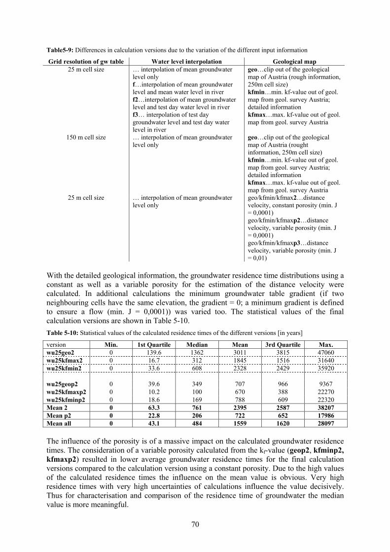
70

Table5-9: Differences in calculation versions due to the variation of the different input information

Grid resolution of gw table Water level interpolation Geological map 25 m cell size … interpolation of mean groundwater

level only f…interpolation of mean groundwater level and mean water level in river f2…interpolation of mean groundwater level and test day water level in river f3… interpolation of test day groundwater level and test day water level in river

geo…clip out of the geological map of Austria (rough information, 250m cell size) kfmin…min. kf-value out of geol. map from geol. survey Austria; detailed information kfmax…max. kf-value out of geol. map from geol. survey Austria

150 m cell size … interpolation of mean groundwater level only

geo…clip out of the geological map of Austria (rought information, 250m cell size) kfmin…min. kf-value out of geol. map from geol. survey Austria; detailed information kfmax…max. kf-value out of geol. map from geol. survey Austria

25 m cell size … interpolation of mean groundwater level only

geo/kfmin/kfmax2…distance velocity, constant porosity (min. J = 0,0001) geo/kfmin/kfmaxp2…distance velocity, variable porosity (min. J = 0,0001) geo/kfmin/kfmaxp3…distance velocity, variable porosity (min. J = 0,01)

With the detailed geological information, the groundwater residence time distributions using a constant as well as a variable porosity for the estimation of the distance velocity were calculated. In additional calculations the minimum groundwater table gradient (if two neighbouring cells have the same elevation, the gradient = 0; a minimum gradient is defined to ensure a flow (min. J = 0,0001)) was varied too. The statistical values of the final calculation versions are shown in Table 5-10. Table 5-10: Statistical values of the calculated residence times of the different versions [in years] version Min. 1st Quartile Median Mean 3rd Quartile Max. wu25geo2 0 139.6 1362 3011 3815 47060 wu25kfmax2 0 16.7 312 1845 1516 31640 wu25kfmin2 0 33.6 608 2328 2429 35920 wu25geop2 0 39.6 349 707 966 9367 wu25kfmaxp2 0 10.2 100 670 388 22270 wu25kfminp2 0 18.6 169 788 609 22320 Mean 2 0 63.3 761 2395 2587 38207 Mean p2 0 22.8 206 722 652 17986 Mean all 0 43.1 484 1559 1620 28097 The influence of the porosity is of a massive impact on the calculated groundwater residence times. The consideration of a variable porosity calculated from the kf-value (geop2, kfminp2, kfmaxp2) resulted in lower average groundwater residence times for the final calculation versions compared to the calculation version using a constant porosity. Due to the high values of the calculated residence times the influence on the mean value is obvious. Very high residence times with very high uncertainties of calculations influence the value decisively. Thus for characterisation and comparison of the residence time of groundwater the median value is more meaningful.

71

Figure 5-52: Cumulative distribution function with consideration of a constant and a variable porosity

Figure 5-53: Histograms of the final calculation versions with a constant (left) and a variable (right) porosity

The cumulative distribution functions of the final calculation version with consideration of a constant porosity and a variable porosity for the calculation of the distance velocity are shown in Figure 5-52. It can be seen that the versions with the more detailed geological information

72

have a more sharp increase in the distribution functions compared to the other version (geo). Using a constant porosity for the calculation of the distance velocity averages in distribution functions with a higher fraction of values with a high groundwater residence time. Using a half life-time approach (assumed half-life time of nitrate: T1/2=730d (2 years) and T1/2=1460d (4 years), which is a value was given as a range in recent publications) a distribution of the share of areas contributing to the nitrogen input to the river was calculated. The calculations based on the assumption of a constant nitrogen input of 25kgN/ha*a at the top of the groundwater layer (consideration of an average denitrification in the soil of 15kgN/ha*a and an average nitrogen surplus of 40kgN/ha*a at the surface of the soil). A reduction of the nitrate in dependency of the residence time and the half life time of nitrate was assumed and nitrogen loads discharged from groundwater to the river were calculated.

Figure5-54: Area-specific and total nitrogen loads calculated from the residence time distributions of the different calculation versions with consideration of half-life-times of 2 years respectively 4 years (area = 100.5 km2)

Figure5-54 shows the area-specific and the total nitrogen loads which were calculated based on the residence time distributions of the final calculation versions varying the porosity and using two different half life times for nitrate. Generally, the area-specific and the total nitrogen loads we estimated to be higher using the raw geological information (geo). The consideration of a variable porosity (p2) instead of a constant porosity (2) resulted in an increase of the total and area-specific nitrogen loads. That increase is, if each calculation version with variable porosity is related to its version with a constant porosity, higher for the calculation versions (kfmin/kfmax: ~ +50%) than for the version (geo: ~ +10%). Obviously the nitrogen emissions increase if the half life times for a nitrate retention is assumed to be higher. Compared to the measurements (in stream loads) in the Wulka river, the half-life time of 4 years results in area-specific loads around 5 kg/ha*a which is quite comparable to the measurements and means, that about 20% of the of the nitrogen input into groundwater reaches the river. Taking into account the statistic values of the average residence time a contradiction appears. The (geo)-versions averagely have a higher residence times, but also higher total and area-specific nitrogen load due to the higher fraction of areas with a low residence time compared to the (kfmin/kfmax)-versions (see Figure 5-55 and Figure 5-56). Generally, an assessment of the calculation versions in terms of a “true” value is not possible. An assessment was done only in a way of a comparison of the calculated N loads in relation to the measured instream loads. For the (geo)-versions most of the nitrogen loads (nearly 90%) stem from areas with a groundwater residence time ≤ 3 years (half life time = 4 years). In the (kfmin/kfmax)-versions only 50-60% of the total nitrogen loads comes from areas with residence times of ≤ 3 years. The contribution of nitrogen is more evenly distributed for the (kfmin/kfmax)-

Halflife-time = 2 years

0

5

10

15

wu25geo

2

wu25k

fmin2

wu25kfm

ax2

wu25ge

op2

wu25k

fminp

2

wu25kfm

axp2

N-lo

ad [k

g/ha

*a]

0

20

40

60

N-lo

ad [t

/a]

area-specific loadtotal load

Halflife-time = 4 years

0

5

10

15

wu25geo2

wu25kfm

in2

wu25kfm

ax2

wu25geop3

wu25kfm

inp3

wu25kfm

axp3

N-lo

ad [k

g/ha

*a]

0

20

40

60

N-lo

ad [t

/a]

area-specific loadtotal load

73

versions, a share of nearly 90% of the total nitrogen load comes from areas with a residence time of ≤ 9-10 years (half life time = 4 years).

Figure 5-55: Contribution of zones of areas according to there groundwater residence time to the total nitrogen emissions via groundwater (calculated as fraction) with the consideration of different half life times

Figure 5-56: Cumulative fraction of areas with a certain residence time on the total area

In regard to this fraction of areas which are the source of most of the nitrogen emissions (residence times of ≤ 9-10 years) Figure 5-56 shows that this fraction covers only 10-25% of the total area. The residual fraction of the total area (mainly areas with a higher distance to the surface water) is due to the higher residence time and the high level of nitrate retention of an insignificant importance in regard to the contribution to the total nitrogen emissions via groundwater to surface waters (see Figure 5-57).

Figure 5-57: Spatial distribution of the areas with their cumulative contribution to the total nitrogen emissions via groundwater to surface waters for two calculation versions (half-life time = 4 years)

Halflife time = 2 years

0

20

40

60

80

100

<1 1 2 3 4 5 6 7 8 >9

Residence time [years]

Cum

ulat

ive

fract

ion

of to

tal a

rea

[%] wu25geo2

wu25kfmin2wu25kfmax2wu25geop2wu25kfminp2wu25kfmaxp2

Halflife time = 4 years

0

20

40

60

80

100

<1 1 2 3 4 5 6 7 8 9 10 11 13 16 >19

Residence time [years]

Cum

ulat

ive

fract

ion

of to

tal a

rea

[%] wu25geo2

wu25kfmin2wu25kfmax2wu25geop2wu25kfminp2wu25kfmaxp2

Halflife time = 2 years

0

10

20

30

40

50

<1 1 2 3 4 5 6 7 8 >9

Residence time [years]

Shar

e [%

]

wu25geo2wu25kfmin2wu25kfmax2wu25geop2wu25kfminp2wu25kfmaxp2

Halflife-time = 4 years

0

10

20

30

40

50

<1 1 2 3 4 5 6 7 8 9 10 11 13 16 >19

Residence time [years]

Shar

e [%

]

wu25geo2wu25kfmin2wu25kfmax2wu25geop2wu25kfminp2wu25kfmaxp2

74

In Figure 5-57 the spatial distribution of the cumulative contribution of the catchment areas to the total nitrogen load is shown. Nearly 97% of the total nitrogen load comes from the areas with a groundwater residence time < 5 (geo2) respectively < 13 years (kfmaxp2) (coloured red to green). This areas cover 10-25% of the total area. That means, that all the blue areas (75-90% of the total considered area) in Figure 5-57 are contributing not more than the remaining 3% of the total nitrogen loads to the rivers. That indicates the importance of the zones near the river systems (up to 2000m) for nitrogen emissions. It has to be mentioned that a constant N-surplus over the whole calculation area was considered for this calculations only.

5.4.2. Ybbs For the Ybbs catchment calculations were performed in a similar way than in the Wulka catchment. The grid resolution of the groundwater table information and the hydraulic conductivities were varied. Additionally, results from more detailed investigations of the groundwater table within a much smaller spatial extend were used for additional calculations (see Figure 5-58). Table5-11 gives an overview on the information that have been modified for the different calculations. Table5-11: Differences in calculation versions due to the variation of the different input information

Grid resolution of gw table Order of river network Geological map 25 m cell size k3…consideration of rivers of the first,

second and third order only k4… consideration of rivers of the first, second, third and fourth order only k5… consideration of rivers of all five orders

geo…clip out of the geological map of Austria (rough information, 250m cell size) kfmin…min. kf-value out of geol. map from geol. survey Austria; detailed information kfmax…max. kf-value out of geol. map from geol. survey Austria

100 m cell size k3…consideration of rivers of the first, second and third order only k4… consideration of rivers of the first, second, third and fourth order only

kfmin…min. kf-value out of geol. map from geol. survey Austria; detailed information kfmax…max. kf-value out of geol. map from geol. survey Austria

10 m cell size, measurements from detailed investigations (datum plates – see Figure

5-58)

k5… consideration of rivers of all five orders

kfmin…min. kf-value / kfmax…max. kf-value out of geol. map from geol. survey Austria

25 m cell size … interpolation of mean groundwater level only

geo/kfmin/kfmax2…distance velocity, constant porosity (min. J = 0,0001) geo/kfmin/kfmaxp2…distance velocity, variable porosity (min. J = 0,0001) geo/kfmin/kfmaxp3…distance velocity, variable porosity (min. J = 0,01)

75

Figure 5-58: Spatial extend of the interpolated groundwater table information (left) out of the groundwater gauging stations (yellow, stations green) and the measurements from datum plates (red-brown)

The spatial extend of the information of the groundwater table is shown in Figure 5-58. The interpolated grid covers only the part downstream of the Ybbs watershed limited by the number and location of groundwater observation wells. The more detailed measurements (datum plates - see general description 5.4) give better information about the spatial distribution of the groundwater level, but they are limited to a much smaller spatial extend. Both information were used for initial calculation of the potential groundwater residence time in the Ybbs catchment. The initial calculations were performed assuming that the distance velocity is equal to the kf-value (means the hydraulic gradient J = 1). The dependencies of the calculated potential residence times from the grid cell size, the order of rivers considered as barriers for the groundwater flow, and the different geological maps are significant. From the initial calculations it arises that the calculated residence times considering only the rivers up to the third order (k3) lead to huge mean residence times for both the 25m grid cell size (y25) and the 100m grid cell size (y100). This is due to the relatively long calculated flow paths of the groundwater because of the absence of the smaller rivers (4th or 5th order) as barriers for the groundwater flow. Unlike these versions the calculated residence times for the grid sizes of 100m (y100) with consideration of rivers up to the 4th order (k4) are much less than those of the 25m grid size (y25). In regard to the used geological maps the consideration of information with low resolution (geo) results generally in a more evenly cumulative distribution function (CDF) of the groundwater residence time than the detailed geological map (kfmin/kfmax). The calculations using the datum plates and the raw geological information (geo) led to a less evenly distributed CDF than the detailed geological information (kfmin/kfmax) due to the small spatial extend and the occurrence of a few geological formations (geo) within this extend only. The initial results indicated that for further calculations a 25m grid cell size, rivers up to the 4th order as barriers for the groundwater flow and the interpolated average groundwater table should be used. With the detailed geological information, the groundwater residence time distributions using a constant as well as a variable porosity for the estimation of the distance velocity were estimated. In additional calculations the minimum groundwater table gradient (if two neighbouring cells have the same elevation, the gradient = 0; a minimum gradient is defined to ensure a flow (min. J = 0,0001)) was varied too. The statistical values of the final calculation versions are shown in Table 5-12.

76

Table 5-12: Statistical values of the calculated residence times of the different versions [in years]

version Min. 1st Quartile Median Mean 3rd Quartile Max. y25k4geo2 0.03 157 800 1756 2192 88330 y25k4kfmin2 0 9.8 29 628 167 101600 y25k4kfmax2 0 6.2 15 222 36 101600 y25k4geop2 0 42 212 457 574 17160 y25k4kfminp2 0 5.4 15 184 67 19070 y25k4kfmaxp2 0 3.6 9 70 21 19070 Mean 2 0 58 281 869 798 97177 Mean p2 0 17 79 237 221 18433 Mean all 0 37 180 553 510 57805 The influence of the porosity is, as already shown for the Wulka catchment, of a massive impact on the calculated groundwater residence time. The consideration of a variable porosity calculated from the kf-value (geop2, kfminp2, kfmaxp2) resulted in lower average groundwater residence times for the final calculation versions compared to the calculation version using a constant porosity. Compared to the Wulka catchment, the calculated residence times are significantly lower for both the versions considering the constant and the variable porosity.

Figure 5-59: Cumulative distribution function with consideration of a constant and a variable porosity

77

Figure 5-60: Histograms of the final calculation versions with a constant (left) and a variable (right) porosity

The cumulative distribution functions of the final calculation versions with consideration of a constant porosity and a variable porosity are shown in Figure 5-59. It can be seen that the versions with the more detailed geological information have a more sharp increase in the distribution functions compared to the other version (geo). Using a constant porosity for the calculation of the distance velocity averages in distribution functions with a higher share of values of a high groundwater residence time. The distributions of the CDF are similar to those calculated for the Wulka catchment, but with a difference in the covered range. For the Ybbs catchment, using the constant porosity lower average residence times were calculated as compared to the Wulka catchment, but with higher maximum values. Using the variable porosity, the average residence times are lower in the Ybbs catchment too, but the maximum values have the same order of magnitude. Using a half life-time approach (assumed half life time of nitrate: T1/2 = 730d and T1/2 = 1460d) a distribution of the share of the contribution of areas to the nitrogen emissions to the river surface waters was calculated. The calculations based on the assumption of a constant nitrogen loss of 50kgN/ha*a from the soils to the groundwater (consideration of a denitrification in the soil and an average nitrogen surplus of 75kgN/ha*a in the soil). A reduction of nitrate in dependency of the residence time and the half life time of nitrate was assumed and nitrogen loads discharged from groundwater to the river were calculated.

78

Figure 5-61: Area-specific and total nitrogen loads calculated from the residence time distributions of the different versions with consideration of half-life-times of 2 years respectively 4 years (area=176 km2)

Figure 5-61 shows the area-specific and the total nitrogen loads which were calculated based on the residence time distributions of the different versions and using two different half life times for nitrate in groundwater. Generally, the total nitrogen loads increase with the increase in resolution of the geological information. The consideration of a variable porosity (p2) resulted in an increase of the total and the specific nitrogen loads compared to the versions using a constant porosity (2). That increase is higher for the (kfmin/kfmax: ~ 50-60%)-versions than for the (geo: ~ 10%)-version. In regard to the assumed half life time the nitrogen emissions increase using a higher half life time for nitrate reduction. Compared to the measurements (in stream loads) in the Ybbs river, the half life time of 4 years results in area-specific loads up to15 kg/ha*a which is comparable to the measurements (18 kg/ha*a) in case of version kfmaxp2 which means, that nearly about 40% of the emissions to the groundwater reach the river via the groundwater. Taking into account the statistic values and Figure 5-59 it is obvious that the total nitrogen load is lower due to the average higher residence times for the (geo)-versions compared to the (kfmin/kfmax)-versions. Generally, an assessment of the calculation versions in terms of a “true” value is not possible. An assessment was done only in a way of a comparison of the calculated N loads in relation to the measured instream loads. The contribution of areas with a certain residence time to the total nitrogen load is shown in Figure 5-62.

Figure 5-62: Contribution of zones of areas according to there groundwater residence time to the total nitrogen emissions via groundwater (calculated as fraction) with the consideration of different half life times

For the (geo)-versions most of the nitrogen loads (nearly 90%) stem from areas with a groundwater residence time ≤ 5-6 years (half life time = 4 years). In comparison with the (kfmin/kfmax)-versions from that areas comes about 73-80% of the total nitrogen load. The

Halflife time = 2 years

0

10

20

30

y25geo2

y25kfm

in2

y25kfm

ax2

y25geop

2

y25kfm

inp2

y25k

fmax

p2

N-lo

ad [k

g/ha

*a]

0

100

200

300

N-lo

ad [t

/a]

area-specific N-loadtotal N-load

Halflife time = 4 years

0

10

20

30

y25geo

2

y25k

fmin2

y25k

fmax

2

y25g

eop2

y25kfm

inp2

y25kfm

axp2

N-lo

ad [k

g/ha

*a]

0

200

400

600

N-lo

ad [t

/a]

area-specific N-loadtotal N-load

Halflife time = 2 years

0

10

20

30

40

50

<1 1 2 3 4 5 6 7 8 9 10 > 11

Residence time [years]

Shar

e [%

]

y25geo2y25kfmin2y25kfmax2y25geop2y25kfminp2y25kfmaxp2

Halflife time = 4 years

0

10

20

30

40

50

<1 1 2 3 4 5 6 7 8 9 10 11 12 13 14 15 17 21 >23

Residence time [years]

Shar

e [%

]

y25geo2y25kfmin2y25kfmax2y25geop2y25kfminp2y25kfmaxp2

79

contribution of nitrogen is more evenly distributed for the (kfmin/kfmax)-versions, the contribution of nearly 90% of the total nitrogen load comes from areas with a residence time of ≤ 8-11 years (half life time = 4 years).

Figure 5-63: Cumulative fraction of areas with a certain residence time on the total area

Figure 5-64: Spatial distribution of the areas with their cumulative contribution to the total nitrogen load for two calculation versions (half-life time = 4 years)

In respect to the fraction of total area which contributes to the nitrogen emissions the versions differ significantly (see Figure 5-63). For the (geo)-versions can be stated that only about 10% of the total area is responsible for nearly 90% of the total nitrogen emissions. For the (kfmin/kfmax)-versions up to 60% of the total area is responsible for nearly 90% of the nitrogen emissions and this fraction is significantly higher as compared to the Wulka catchment. The residual fraction of the total area (mainly areas with a higher distance to the surface water) are of a low importance in regard to the contribution to the total nitrogen emissions because of to the higher residence time and the high level of nitrate retention. In Figure 5-64 the spatial distribution of the cumulative contribution of the catchment areas to the total nitrogen load is shown. Nearly 97% of the total nitrogen load comes from areas with a groundwater residence time < 10 (geo2) and < 13 years (kfmaxp2), respectively. These areas cover a fraction of 10 (geo2) -60 (kfmaxp2) % of the total considered area. That means, that all the blue areas (40-90% of the total area) in Figure 5-64 contribute only with 3% of the total nitrogen loads to the rivers. Especially for the (geo)-versions the importance of the river near areas for the contribution to the nitrogen emissions is obvious.

Halflife time = 2 years

0

20

40

60

80

100

<1 1 2 3 4 5 6 7 8 9 10 > 11

Residence time [years]

Cum

ulat

ive

fract

ion

of to

tal a

rea

[%] y25geo2

y25kfmin2y25kfmax2y25geop2y25kfminp2y25kfmaxp2

Halflife time = 4 years

0

20

40

60

80

100

<1 1 2 3 4 5 6 7 8 9 10 11 12 13 14 15 17 21>2

3

Residence time [years]

Cum

ulat

ive

fract

ion

of to

tal a

rea

[%] y25geo2

y25kfmin2y25kfmax2y25geop2y25kfminp2y25kfmaxp2

80

5.4.3 Summary Deductively the following main statements in regard to the calculation procedure can be drawn from the calculations in both catchments

• the order of rivers that are considered as groundwater flow barriers is of a large importance for the calculation of the groundwater residence time

• the grid cell size of the interpolated groundwater table information affects the residence time calculations

• the differences in information about the geology (degree of details) influence the calculations of the groundwater residence time

• due to variations of the calculated mean groundwater residence time and the comparison of the calculated N loads with measured instream N loads for the calculation of the groundwater residence time the 25m grid cell size is recommended

• the use of the variable porosity for the calculation of the distance velocity seems to be more appropriate than using a constant value; limitations for the groundwater table gradient (minimum values) do affect the calculated groundwater residence time distribution significantly

In regard to the calculated nitrogen emissions to the river can be concluded: • the assumed average half life time of 4 years for a nitrate reduction resulted in

nitrogen loads that are comparable to the measured in stream loads in the Wulka catchment

• for the Ybbs catchment average a half-life time of 4 years resulted in nitrogen emissions via groundwater that are lower than the measured in stream loads, the assumption of high half life times would result in better fits between measured and calculated values

• nearly all the nitrogen emissions via groundwater stem from areas with a distance of up to 2500 m upstream (groundwater) of the river system and with relative low average groundwater residence time (up to 13 years), this indicates the importance of these areas in regard to land management

It has to be mentioned that due to the uncertainties of the input information these calculations have high uncertainties concerning the quantitative conclusion. But in a more qualitative way they can very clearly point out the relation between nitrogen surpluses on the areas, residence times in groundwater and the contribution of areas to the nitrogen emissions to surface water via groundwater.

5.5. Nutrient surplus and content in agriculture soils

5.5.1. Nutrient surplus in agricultural soils Calculations of the surplus in agricultural soils were done based on statistical and literature data on the level of municipalities for a time span of almost 40 years (1964 to 1999). In between balances were calculated in time steps of 5 to 10 years dependent on the availability of the statistical data. As input fluxes into the soils application of mineral fertiliser, manure and sewage sludge as well as biological nitrogen fixation and deposition were considered. Outputs from the agricultural soils are nutrients in harvested products and the ammonia losses from manure after application. In addition potential influence of the stable nitrogen pool on the yearly balance was estimated with the calculation of the nitrogen net mineralization. Assumptions for the calculations of nutrient fluxes based on the statistical data are summarised in the Annex. Calculated surpluses are either denitrified or leached to the groundwater.

81

Problematic are the data for mineral fertiliser application. In Austria till 1995 information on the selling of mineral fertiliser on the district level exist. The problem with these data is, that especially in districts with larger towns the sales statistic may not coincident with the application. Since 1995 only data for fertiliser application on the level of federal states are published. Therefore following procedure has been applied. On the one hand the trend of the development of fertiliser use on federal state level since 1995 was assumed for the district level. Average sales statistics were used for application values on regional basis. On the other hand based on crop statistics the needed amount of fertiliser was calculated on municipal level assuming an application based on the guidelines for fertiliser applications in Austria. It was assumed that the fertiliser application lies between this target value and up to 20 % more. Finally the fertiliser application based on sales statistics together with availability of manure in a municipality was compared with the amount of fertiliser needed based on guidelines and the higher value was assumed to be the total fertiliser application in the municipality. The manure application was calculated based on a transformation of the number of animals to animal units and specific nutrient contents in manure for the animal units. The amount of sewage sludge application was calculated in a way that for those treatment plants where sewage sludge is used in agriculture it was assumed that the sludge was equally distributed on the agricultural areas of the municipalities discharging their waste water to the treatment plant. For the biological nitrogen fixation it was assumed that the nitrogen in the harvested products from legumes stems from fixation. In respect to deposition data from measurements of wet deposition of stations in the region or close to the region were taken. For the dry deposition estimations from literature were used. The nutrient content in harvested products was calculated based on literature data of nutrients in harvested products, the land use statistics (area used for production of certain crops) on municipality level and the statistics on crop yields which is available on district level. Ammonia losses from applied manure again were estimated based on specific values for animal units. The nitrogen net mineralization was calculated based on the approach in the “Stoffbilanz” model (Gebel, 2003). In this model it is assumed that 50 % of the applied manure is going to the stable nitrogen pool and a mineralization from the stable nitrogen pool is calculated based on the soil type and the planted crops. Wulka Agriculture in the Wulka catchment is characterised by a low animal density. Production is dominated by crop production and not by production of animal products. That leads to a high share of mineral fertiliser application. The sewage sludge supplies about 2 % of nitrogen and 5 % of phosphorus. The surplus on agricultural soils is relatively equal distributed over the catchment. Only in one municipality the surplus is significantly higher than in the others. 25 % of the animal husbandry is located here. As average over the whole catchment net mineralization tends to increase the available nitrogen and reduces the stable soil nitrogen pool and increases the yearly surplus.

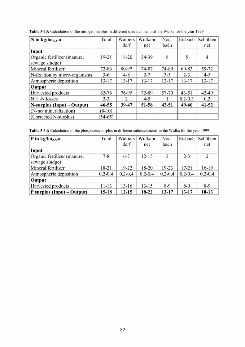
82

Table 5-13: Calculation of the nitrogen surplus in different subcatchments at the Wulka for the year 1999

N in kg/haAA.a Total Walbers dorf

Wulkapr net

Nod-bach

Eisbach Schützen net

Input Organic fertilizer (manure, sewage sludge)

19-21 18-20 34-39 8 5 4

Mineral fertilizer 72-86 80-97 74-87 74-89 69-83 59-72 N-fixation by micro-organisms 3-6 4-8 2-7 3-5 2-3 4-5 Atmospheric deposition 13-17 13-17 13-17 13-17 13-17 13-17 Output Harvested products 62-76 76-95 72-89 57-70 43-51 42-49 NH3-N losses 2-3 2 4-5 1 0,2-0,3 0,2 N-surplus (Input – Output) 46-55 39-47 51-58 42-51 49-60 41-52 (N-net mineralization) (8-10) (Corrected N-surplus) (54-65)

Table 5-14: Calculation of the phosphorus surplus in different subcatchments in the Wulka for the year 1999

P in kg/haAA.a Total Walbers dorf

Wulkapr net

Nod-bach

Eisbach Schützen net

Input Organic fertilizer (manure, sewage sludge)

7-8 6-7 12-15 3 2-3 2

Mineral fertilizer 18-21 19-22 18-20 19-23 17-21 16-19 Atmospheric deposition 0,2-0,4 0,2-0,4 0,2-0,4 0,2-0,4 0,2-0,4 0,2-0,4 Output Harvested products 11-13 13-16 13-15 8-9 8-9 8-9 P surplus (Input – Output) 15-18 12-15 18-22 13-17 13-17 10-13

83

Figure 5-65: Regional distribution of nitrogen surpluses in the Wulka catchment for the year 1999

0

20

40

60

80

100

120

1964

1966

1968

1970

1972

1974

1976

1978

1980

1982

1984

1986

1988

1990

1992

1994

1996

1998

2000

N s

urpl

us (k

g/ha

.a)

NodbachWulkaprod. totalSchützen total

0

200

400

600

800

1000

1200

1964

1966

1968

1970

1972

1974

1976

1978

1980

1982

1984

1986

1988

1990

1992

1994

1996

1998

P ac

cum

ulat

ion

(kg/

ha)

NodbachWulkaprod. totalSchützen total

Figure 5-66: Development of nitrogen surpluses in the Wulka catchment

Figure 5-67: Phosphorus accumulation in the Wulka catchment

The nitrogen surplus in the Wulka catchment in 1999 was the lowest since 1964. Till the early eighties it was increasing but it is decreasing till than. The reason for this is, that the animal density is decreasing since the sixties, since the late eighties mineral fertiliser application is decreasing as well. Phosphorus accumulation in the soils is going on since the sixties. Based on natural near soil contents in the early sixties this accumulation was used to estimate average actual concentrations. Results are shown in Table 5-15.

84

Table 5-15: Average P concentrations in agricultural soils in the fifties (“natural near”) and in the late nineties calculated based on MONERIS assumptions

“Natural near” concentrations

(MONERIS) Average concentrations

1999 [mgP/kg] [mgP/kg]

Walbersdorf 355 739 Wulkaprodersdorf 403 778 Eisbach 426 649 Nodbach 385 658 Schützen 394 607

Ybbs The situation in the Ybbs catchment is different from the Wulka. The upstream parts are characterised by extensive animal husbandry more downstream the cattle density is significantly increasing. Organic fertiliser (mainly manure) is dominating the nutrient inputs into the soils. In the upstream part surpluses of nutrients in soils are small, but much higher in the more downstream parts. Municipalities with the highest animal density have the highest surpluses in agricultural soils. Table 5-16: Calculation of the nitrogen surplus in different subcatchments at the Ybbs for the year 1999

N in kg/haAA.a Total Opponitz Url/ Krenstetten

Greimperd. net

Input Organic fertilizer (manure, sewage sludge)

109-123 57-68 128-144 108-122

Mineral fertilizer 35 36-39 42 37 N-fixation by micro-organisms 7-8 0-1 10-13 7-8 Atmospheric deposition 20-24 14-18 20-28 18-22 Output Harvested products 105-119 78-93 98-124 82-102 NH3-N losses 10-16 6-9 13-20 11-16 N-surplus (Input – Output) 72-74 23-24 85-90 71-77 (N-net mineralization) (-(24-32) (Corrected N-surplus) (48-42)

Table 5-17: Calculation of the phosphorus surplus in different subcatchments in the Ybbs for the year 1999

P in kg/haAA.a Total Opponitz Url/ Krenstetten

Greimperd. Net

Input Organic fertilizer (manure, sewage sludge)

28-37 9-13 32-43 27-36

Mineral fertilizer 10-11 19-21 9-10 12 Atmospheric deposition 0,2-0,4 0,2-0,4 0,2-0,4 0,2-0,4 Output Harvested products 17-20 15-18 19-23 16-19 P surplus (Input – Output) 21-28 14-17 24-31 25-32

85

Figure 5-68: Regional distribution of nitrogen surpluses in the Ybbs catchment for the year 1999

The nitrogen surplus sharply increased in the seventies, reached its maximum in the early eighties and is slowly decreasing since. Phosphorus accumulation was the fastest in the late seventies and the eighties. Accumulation still takes place but significantly slower than in the eighties. Calculations of average P-concentrations in soil based on long term surpluses lead to lower values for the upstream parts and higher values for the downstream parts as compared to the Wulka catchment.

0

20

40

60

80

100

120

1964

1966

1968

1970

1972

1974

1976

1978

1980

1982

1984

1986

1988

1990

1992

1994

1996

1998

N s

urpl

us (k

g/ha

.a)

KrenstettenOpponitzGreimpersdorf

0

200

400

600

800

1000

1200

1964

1966

1968

1970

1972

1974

1976

1978

1980

1982

1984

1986

1988

1990

1992

1994

1996

1998

P a

ccum

ulat

ion,

kg/

ha

KrenstettenOpponitzGreimpersdorf

Figure 5-69: Development of nitrogen surpluses in the Wulka catchment

Figure 5-70: Phosphorus accumulation in the Wulka catchment

86

Table 5-18: Average P concentrations in agricultural soils in the fifties (“natural near”) and in the late nineties calculated based on MONERIS assumptions

“Natural near” concentrations

(MONERIS) Average concentrations

1999 [mgP/kg] [mgP/kg]

Opponitz 422 595 Krenstetten 355 806 Greimpersdorf 396 832

5.5.2. Nutrient concentration in soils Three data sources were investigated for N and P concentrations in the soils:

• Measurements of plant available P in soils in various regions in Lower Austria (paPs) • State inventory of soils (BZI = Bodenzustandsinventur) • Soil measurements in the district of Amstetten at sites where sewage sludge is applied

Ad Measurements of plant available P in soils in various regions in Lower Austria (paPs): In this data base mean concentrations of plant available P in agricultural soils in various municipalities and the related number of single samples are included. There is no clear distinction between meadows or arable land. Therefore we used the relation of arable land to meadows to categorize the data. E.g. all values given for municipalities with a share of less than 6 % arable land were categorized as meadows. However, as we will see below, the run of the curve of the potential regression equation between the plant available P and Ptotal for arable land and meadows is quite similar (Figure 5-71 and Figure 5-72). For the category meadows (defined as: less than 6 % arable land) we finally obtained 11 mean values, based on 1189 single samples. For the category arable land (defined as: more than 50% arable land) we finally obtained 12 mean values, based on 2317 single samples. ad. BZI: For the BZI inventory samples are taken from soils in a 4 x 4 km grid all over Austria. In total for the Ybbs catchment 70 and for the Wulka 13 data sets were available. Information was retrieved on the category (forest, arable land, meadows, wine yard) and on the nutrient content. For all categories total N was provided. Total P was only given for the category forest. For arable land, meadows and wine yards only the plant available P fraction was given. This P fraction was transferred into total P using the regression equation presented below. ad. Soil measurements in the district of Amstetten at sites where sewage sludge is intended to be applied: Before the application of sewage sludge on fields the related soils have to be investigated if they are appropriate for the application of sludge. From the sewage treatment plant of Amstetten we obtained 305 results of these investigations. Out of these 269 results stem from arable land and 188 of them lie within the catchment of the Ybbs as far as it is considered in this investigations. This data base includes no N-concentrations but Ptotal as well as plant available P. These data sets were used to derive correlations between Ptotal and plant available P. Using a linear regression equation the correlation coefficient was r2 = 0,71. In order to improve the fitting in a first step the ratio of Ptotal : plant available P was calculated. This ratio further on was used in a second step to compare it with the plant available P. A much better fitting of the regression equation was achieved using a potential equation: the correlation coefficient increased to r2 = 0,89 for arable land (see Figure 5-71).

87

arable land all data sets

y = 35,951x-0,726

R2 = 0,8926

0

5

10

15

20

25

30

35

40

45

0 20 40 60 80 100 120 140

content P2O5 mg/100g

rela

t. P

tot t

o P

2O5

relation P2O5:Ptot arable land Potenziell (relation P2O5:Ptot arable land)

Figure 5-71: ratio of Ptot to P2O5 in arable land (data sets “Amstetten”)

The same procedure was done for meadows. Using a potential equation a correlation coefficient of r2 = 0,91 was achieved.

meadows all data sets

y = 55,868x-0,8569

R2 = 0,9097

0

5

10

15

20

25

30

0 2 4 6 8 10 12 14 16 18

mg P2O5/100g

rela

tion

Ptot

to P

2O5

meadows Potenziell (meadows)

Figure 5-72: ratio of Ptot to P2O5 in meadows

With these potential regression equations the values given in the other two data sources were converted to Ptotal. In the following tables the results for N and Ptotal are depicted, subdivided if possible to subcatchments.

88

Table 5-19: N concentration in soils according the soil inventory (BZI)

forest wine arable l. forest arable l.0-10 cm 0-5 cm 0-20 cm 0-20 cm 0-20 cm 0-10 cm 0-5 cm 0-20 cm 0-20 cm

number 2 1 1 6 12 11 25 41 21mean value 0,26 0,19 0,17 0,14 0,15 0,83 0,49 0,39 0,18min 0,24 0,19 0,17 0,1 0,1 0,25 0,05 0,13 0,12max 0,28 0,19 0,17 0,18 0,2 1,90 1,24 0,79 0,38

forest arable l. forest arable l. forest0-10 cm 0-5 cm 0-20 cm 0-20 cm 0-10 cm 0-5 cm 0-20 cm 0-20 cm 0-10 cm 0-5 cm 0-20 cm

number 1 5 9 9 3 12 24 12 7 8 8mean value 0,25 0,42 0,28 0,17 0,42 0,44 0,36 0,20 1,09 0,60 0,58min 0,22 0,13 0,13 0,32 0,31 0,22 0,12 0,25 0,05 0,25max 0,58 0,38 0,26 0,62 0,77 0,79 0,38 1,90 1,24 0,79

N tot in %

Krenstetten Greimpersdorf Opponitzmeadows meadows meadows

N tot in %

Wulka Ybbsmeadows meadows

Table5-20: Ptot concentrations according various data sources (paPs: plant available P in soils; BZI: State inventory of soils)

mg Ptot/kg paPs BZI paPs BZI Amstetten paPs BZI Amstettennumber 1779 12 1376 12 124 941 8 51mean value 707 730 579 649 753 607 676 825min 591 590 550 515 408 552 499 454max 783 951 632 812 1004 766 915 1193

mg Ptot/kg BZI paPs BZI Amstetten paPs BZI Amstetten paPs BZInumber 1 94 17 5 1 5 4 985 15mean value 678 673 619 812 709 668 794 680 605min 645 490 668 573 469 578max 718 844 965 792 727 708

arable land Wulka

Wulka YbbsKrenstetten

KrenstettenYbbs

Opponitz

Greimpersdorf

Greimpersdorfmeadows

89

6. MONERIS application

6.1. Methodological aspects The MONERIS application for the Ybbs and Wulka catchment was based on the model description (Behrendt, 1999), excel sheets prepared by the IGB-Berlin and personal communication with Horst Behrendt and Heide Schreiber from IGB-Berlin. The MONERIS model has already been described within the daNUbs project in deliverable D 5.5 “draft regional emission model”. The description is not repeated here. Data used as input data are described in the chapters before. The time period for emission calculations is the 1998 – 2002. Emissions are compared to the transported loads of this period.

6.2. Results Table 6-1 and Figure 6-1 show the results of nutrient emissions via different pathways into the different subcatchments of the Ybbs and the Wulka catchment calculated with the MONERIS model. Results are shown for total subcatchments not only for the net catchments in cases were another subcatchment is located upstream. For nitrogen groundwater is a main pathway in all considered subcatchments. Point sources and tile drainage are important in some the catchments as well. Other pathways are of minor importance. The area specific emissions are much higher in the Ybbs catchment than in the Wulka catchment. Main reasons are not the differences in surpluses in agricultural soils but the much higher retention (denitrification) of nitrogen in the groundwater. For phosphorus erosion is the dominant pathway in all subcatchments except the most upstream located subcatchment in the Ybbs catchment (Opponitz). In some subcatchments point sources contribute with a decisive part. Urban areas contribute with less than 10 % of the emissions in all subcatchments. In the different subcatchments of the Ybbs emissions by groundwater and overland flow have to be considered as well. Area specific phosphorus emissions are similar in the different subcatchments of Wulka and Ybbs. Higher sediment loads in the Ybbs are compensated by higher phosphorus concentrations in suspended solids in the Wulka. Table 6-1: Summary of nutrient emissions (N+P) via pathways calculated based on MONERIS approach for the Ybbs and Wulka catchment including subcatchments

Emission estimates nitrogen catchment area name

Deposi-tion

overland flow

tile drainage

Ero-sion

Ground-water

WWTP urban systems

total N

river load 1998-2002

[t/a] [t/a] [t/a] [t/a] [t/a] [t/a] [t/a] [t/a] TN [t/a]

DIN [t/a]

Wulka Walbersdorf 0,4 0,1 5,0 2,1 25,2 2,9 1,7 37 23 18 Wulkaprod. tot. 1,2 0,2 21,0 11,2 79,6 5,5 3,2 122 77 59 Eisbach 0,6 0,0 8,6 2,5 12,5 18,8 1,6 45 47 41 Nodbach 0,3 0,0 8,4 1,3 6,2 0,0 0,7 17 12 8 Schützen total 2,4 0,2 49,3 16,2 99,3 42,6 6,1 216 142 128 Ybbs Opponitz 4,1 30,5 24,2 5,8 722,8 6,7 4,8 799 770 495 Krenstetten 1,1 7,7 25,0 6,0 272,6 38,0 6,4 357 352 293 Greimpersd. tot 12,5 67,0 158,4 38,4 1869,0 75,5 36,0 2257 2065 1895

90

Emission estimates phosphorus catchment area name

Deposi-tion

overland flow

tile drainage

Ero-sion

Ground-water

WWTP urban systems

total P

river load 1998-2002

[t/a] [t/a] [t/a] [t/a] [t/a] [t/a] [t/a] [t/a] TP [t/a] Wulka Walbersdorf 0,0 0,0 0,0 2,4 0,2 0,1 0,3 3,1 1,8 Wulkaprod. tot. 0,0 0,0 0,1 13,6 0,5 0,2 0,7 15,0 3,0 Eisbach 0,0 0,0 0,0 2,5 0,0 1,1 0,3 4,1 2,5 Nodbach 0,0 0,0 0,1 1,3 0,2 0,0 0,2 1,8 0,6 Schützen total 0,1 0,1 0,3 18,5 0,7 3,3 1,3 24,2 7,2 Opponitz 0,10 2,8 0,3 1,4 7,7 1,0 0,8 14 16 Krenstetten 0,02 1,2 0,1 4,4 1,5 1,6 0,8 10 9 Greimpersd. tot 0,25 8,1 0,8 20,5 15,0 12,0 5,0 62 84

0

5

10

15

20

25

Walbersdo

rf

Wulkapro

dersd

orfOslip

St. Marga

rethe

n

Schütze

n

Oppon

itz

Krenste

tten

Greimpers

dorf

Nitro

gen

emis

sion

s (k

g N/

(ha.

a))

urban aereasWWTPgroundwatererosiontile drainageoverland flowDeposition

Wulka Ybbs

0%

20%

40%

60%

80%

100%

Walbersdo

rf

Wulkapro

dersd

orfOslip

St. Marga

rethe

n

Schütze

n

Oppon

itz

Krenste

tten

Greimpers

dorf

Nitr

ogen

sha

re o

f pat

hway

s (%

)

urban aereasWWTPgroundwatererosiontile drainageoverland flowDeposition

Wulka Ybbs

0,0

0,1

0,2

0,3

0,4

0,5

0,6

0,7

0,8

Walbersdo

rf

Wulkapro

dersd

orfOslip

St. Marga

rethe

n

Schütze

n

Oppon

itz

Krenste

tten

Greimpers

dorf

Phos

phor

us e

mis

sion

s (k

g N

/(ha.

a))

urban aereasWWTPgroundwatererosiontile drainageoverland flowDeposition

Wulka Ybbs

0%

10%

20%

30%

40%

50%

60%

70%

80%

90%

100%

Walbers

dorf

Wulkaprode

rsdorf

Oslip

St. Marga

rethen

Schütz

en

Oppon

itz

Krenste

tten

Greimpe

rsdorf

P, s

hare

of p

athw

ay (%

) urban aereasWWTPgroundwatererosiontile drainageoverland flowDeposition

Wulka Ybbs

Figure 6-1: Graphical presentation of nutrient emissions (N+P) via pathways calculated based on MONERIS approach for the Ybbs and Wulka catchment including total subcatchments

In Table 6-2 and Figure 6-2 nutrient emissions are sorted according to activities. Agriculture followed by waste water management (point sources and urban areas) are the main activities leading to nutrient emissions in most of the subcatchments. Background and combustion (for nitrogen) are relevant especially in the Ybbs catchment.

91

Table 6-2: Nutrient emissions by activities in different subcatchments of the Wulka and Ybbs catchment

1998-2002 Nitrogen river name catchment area

name background agriculture point sources +

urban areas other diffuse

sources total

kg/(ha.a) kg/(ha.a) kg/(ha.a) kg/(ha.a) kg/(ha.a)Wulka Wulka Walbersdorf 0,5 3,5 0,6 0,3 4,9 Wulka Wulkaprodersdorf 0,5 4,3 0,4 0,4 5,6 Eisbach Eisbach 0,3 3,3 3,2 0,2 7,0 Nodbach Nodbach 0,2 3,1 0,1 0,1 3,6 Wulka Schützen 0,4 3,7 1,3 0,3 5,6 Ybbs Ybbs Opponitz 4,4 7,6 0,2 3,6 15,8 Url Krenstetten 1,7 17,2 2,9 1,8 23,6 Ybbs Greimpersdorf 3,3 13,3 1,0 2,8 20,4

1998-2002 Phosphorus river name catchment area

name background agriculture point sources +

urban areas other diffuse

sources total

kg/(ha.a) kg/(ha.a) kg/(ha.a) kg/(ha.a) kg/(ha.a)Wulka Wulka Walbersdorf 0,04 0,32 0,05 0,41 Wulka Wulkaprodersdorf 0,03 0,62 0,04 0,69 Eisbach Eisbach 0,03 0,39 0,23 0,64 Nodbach Nodbach 0,05 0,30 0,03 0,38 Wulka Schützen 0,03 0,48 0,12 0,63 Ybbs Ybbs Opponitz 0,18 0,06 0,03 0,28 Url Krenstetten 0,15 0,32 0,16 0,64 Ybbs Greimpersdorf 0,18 0,22 0,15 0,56

0%

20%

40%

60%

80%

100%

Walbersd

orf

Wulkapro

dersdorf

Eisbac

h

Nodbac

h

Schütz

en

Opponit

z

Krenste

tten

Greimpe

rsdorf

N, s

hare

of a

ctiv

ity (%

)

background agriculturepoint sources and urban areas combustion

Wulka Ybbs

0%10%20%30%40%50%60%70%80%90%

100%

Walbersdo

rf

Wulkapro

dersd

orf

Eisbach

Nodbac

h

Schütze

n

Oppon

itz

Krenste

tten

Greimpers

dorf

P, s

hare

of a

ctiv

ity (%

)

background agriculture point sources and urban areas

Wulka Ybbs

Figure 6-2: Relative share of nutrient emissions by activities (Wulka and Ybbs catchment)

In Figure 6-3 the retention expressed as the relation between measured TN and TP loads to calculated TN and TP emissions is plotted against the specific runoff and the hydraulic load of different subcatchments at the Wulka and the Ybbs. The specific runoff of a region is the mean discharge in the river subdivided by the catchment area. The hydraulic load is the discharge in the river subdivided by the surface water area of the catchment. According to the MONERIS model the retention of N and P in surface water is a function of the specific runoff and/or the hydraulic load. The expected retention is printed as a line in the figures. The dotted lines show the expected variation of the retention.

92

Results form emission estimates as compared to river loads show no significant retention of nitrogen or phosphorus in the Ybbs catchment. This is well in line with the expectations based on the MONERIS approach. In one case emissions seem to be underestimated as compared to the measured load (TP-load/TP-emissions > 1). A reason might be the high TP-loads transported during two high flow events in the considered time period. In the Wulka emission estimates which are clearly higher than measured in stream loads indicate retention in the river system. For nitrogen this retention fits well to the retention that would be expected with the retention figures based on the hydraulic load. Only one subcatchment is not in line with the expectations. In this case a significant point source influence upstream the reference point might be the reason for a retention smaller than expected. For TP a deviation can be recognised between the expected retention and the observed retention. While compared to the retention expected based on the specific runoff the observed retention is to low, compared to the retention expected based on the hydraulic load the observed retention is to high.

0,00

0,25

0,50

0,75

1,00

1,25

1,50

1 10 100specific runoff [l/(km²*s)]

TP-lo

ad/T

P-e

mis

sion

Wulka

Ybbs

0,00

0,25

0,50

0,75

1,00

1,25

1,50

1 10 100

specific runoff [l/(km²*s)]

TN-lo

ad/T

N-e

mis

sion

Wulka

Ybbs

0,00

0,25

0,50

0,75

1,00

1,25

1,50

1 10 100 1000

hydraulic load [m/a]

TN-lo

ad/T

N-e

mis

sion Wulka

Ybbs

0,00

0,25

0,50

0,75

1,00

1,25

1,50

1 10 100 1000

hydraulic load [m/a]

TP-lo

ad/T

P-em

issi

on WulkaYbbs

Figure 6-3: Retention versus hydraulic load and area specific runoff for different subcatchments

7. Swat application In D 1.1 already the calibration and the validation of the SWAT 2000 model was presented. Changes arised from the extension of the calculation period due to the acquisition of additional runoff data. Thus, the calculation period covers a time span of 1991-2000 for the Wulka catchment respectively 1991-2001 for the Ybbs catchment. Additionally, for the Wulka catchment a new soil map was introduced to the model. This resulted in changes in the parameter definition for the soil definition, the tile drainage definitions and surface runoff definitions. On basis of t he model definitions from the water balance calculations (and the changes were mentioned) the SWAT 2000 model was further used for nutrient balance calculations for the Wulka and the Ybbs catchment. Changes or new model definitions were necessary are discussed in the following chapter.

93

7.1. Methodology The SWAT 2000 model is able to simulate nutrient turnover and nutrient emissions from the watershed. Effects of fertiliser application, the influence of wwtps, the soil characteristics, nitrogen surplus distributions (on the HRU-level), enrichment ratios for nitrogen and phosphorus and concentrations of nitrogen and phosphorus in the groundwater can be considered. Detailed explanations are given subsequently. Nitrogen The SWAT 2000 model is able to consider nitrate, ammonia and organic nitrogen (fresh organic nitrogen, active organic nitrogen and stable organic nitrogen) and the turnover between these substances in the soil. The following processes are modelled: Table 7-1: Nitrogen turnover is modelled by the SWAT 2000 model

Process Description Model restrictions Decomposition Breakdown of fresh org. N in first layer only,

T > 0°C Mineralization (net) Conversion of org. N to inorg. N in first layer only,

C : N < 20 : 1 T > 0°C

Immobilisation Conversion of inorg. N to org. N C : N > 30 : 1 Nitrification Conversion of NH4 to NO3 T > 5°C Volatilisation Gaseous loss of NH3 T > 5°C Denitrification Conversion of NO3 to N2 soil water content >0.95,

in soil profile only N in rainfall Nitrate added to the soil by rainfall in the top 10mm only Fixation Nitrogen fixation by legumes Leaching Leaching from soil by surface runoff and

lateral flow The movement of nitrogen is modelled in the following way:

Nitrate: by surface runoff (top 10mm only), lateral runoff and percolation (to underlying layer)

Org. N: by surface runoff (attached to soil particles) Phosphorus As well as the nitrogen the turnover of phosphorus is considered in the SWAT 2000 model. Organic phosphorus (fresh organic phosphorus, active organic phosphorus and stable organic phosphorus) and mineral phosphorus (stable mineral phosphorus, active mineral phosphorus and soluble mineral phosphorus ) and the turnover between these substances. The following processes are modelled:

94

Table 7-2: Phosphorus turnover is modelled by the SWAT 2000 model

Process Description Model restrictions Decomposition Breakdown of fresh org. P T > 0°C Mineralization (net) Conversion of org. P to inorg. P T > 0°C Immobilisation Conversion of inorg. P to org. P Sorption Sorption of inorg. P Leaching Leaching from soil from top 10mm to first

layer only The movement of phosphorus is modelled in the following way: Sol. P: by surface runoff (top 10mm only) Org. + min. P: by surface runoff (attached to soil particles) Fertilizer application On basis of the fertilizer statistics on the community level for both catchments the fertilizer use was defined in the SWAT 2000 model. A differentiation between the use of mineral fertilizer and manure was made for the subcatchments of both catchments. The fertilizer application was defined in relation to the potential heat units of the crops. They are used to define several stages of the plant growth in dependency of the heat units were consumed. Three times a year a fertilizer application was defined. For the Wulka catchment, the fertilizer application consists of two mineral and one organic fertilizer application per year. For the Ybbs catchment, the fertilizer application consists of two organic and one mineral fertilizer application per year. Groundwater concentration The concentrations of nitrogen and phosphorus in the groundwater that enters the stream can be specified in the groundwater file. For both catchments the nitrogen and phosphorus concentration in the groundwater was defined on the basis of the groundwater quality measurements with variation for every subcatchment. Initial nutrient concentrations in the soil The SWAT 2000 model offers the possibility to define a initial soil nutrient concentration. Initial calculations showed that defining that initial soil nutrient concentrations result in extraordinary high rates of denitrification in the soil within the first year. Thus, in the following calculations the initial soil nutrient concentrations were not considered anymore. Nitrogen and phosphorus enrichment ratio On basis of literature values (deliverable D. 2.1) the enrichment ratios for organic nitrogen and organic phosphorus (ratio of the concentration transported with the sediment to the concentration of the soil surface layer) were defined with variation for both catchments only. Nitrogen in rainfall On the basis of measurement of the deposition rate the concentration of nitrogen in the rainfall was defined with differentiation between the two catchments only.

95

Contributions of the wwtp’s Based on the measurements of the effluents of the wwtps the nutrient loads to the rivers were considered for both catchments. Further important model parameter In regard to the nitrogen and phosphorus turnover there are further important model parameters which influence the simulation of nutrient cycle by the SWAT 2000 model:

• temperature (see table 7.11/7.12) • water content in the soil layer • bulk density of the soil layer • content of organic carbon in the soil layer • fraction of porosity from which anions are excluded (nitrate transport) • Humus mineralization factor for active organic nitrogen • Plant uptake distribution factors for nitrogen and phosphorus • Percolation coefficients for nitrogen and phosphorus • Phosphorus soil partitioning and sorption coefficient

The mentioned parameters were considered in the calculations.

7.2. Results

7.2.1. Wulka Using the SWAT 2000 model nutrient balances for the Wulka catchment were calculated. The mentioned parameter were defined in the previously mentioned way. Due to the consideration of tile drained areas and a more detailed soil map the model performance decreased significantly indicating a parameter definition which is not sufficient in terms of the reflection of “real circumstances”. In deliverable D1.1 already the difficulties in model parameter definition were discussed. The number of model parameter have to be defined and the possible combinations of parameter sets lead to similar results which makes it difficult to succeed in an optimal model parameterisation. The decrease in the model performance with an increase in the resolution and detail of information of the data indicate a wrong parameterisation of the model, but with a reliable behaviour. After the introduction of the new data to the SWAT 2000 model the model performance decreased from NSC = 0.36 (see D. 1.1) to NSC = -1.86. Despite of additional model calibration the model performance couldn’t be increased. Due to the poor model performance it is quite doubtful whether the presented results can be used for a balance of the nutrients turnover in the catchments. Additionally, not all the flow components are modelled by the SWAT model that are important for calculations of the nitrogen or phosphorus emissions to surface waters. This is, i.e. the case for runoff from tile drained areas. In the Wulka catchment the contribution from tile drained areas to the total runoff is quite important. Another major deficiency of the model is that the nitrogen retention by denitrification is considered in the soil layers only and the nitrate percolates out of soil is not tracked through the aquifer. This makes a balance quite difficult or nearly impossible. The time which was spent on additional model calibration and parameter definition justifies the presentation of the results obtained with the SWAT 2000 model even if results are by far not satisfactory. Taking the mentioned deficiencies into consideration the following nitrogen

96

(Figure 7-1) and phosphorus balance (Figure 7-2) for the Wulka catchment were calculated. On basis of the actual model parameterisation the major nitrogen load stem from soluble nitrogen (nitrate) transported by the lateral flow which is considered to be part of the groundwater flow and stem from point source contribution. The major importance of the contribution of the point sources is obvious. The calculated denitrification rates which take place in the soil profile are unrealistically high. Activities to reduce the results of calculation to realistic values were not that successful. On the other hand the calculated nutrient uptake by plants is unrealistic low. Thus the performance of the model for nutrient balance calculations is very poor for the moment. In regard to the phosphorus balance (Figure 7-2) that was estimated using the SWAT 2000 model it is obvious that by far the highest fraction of the phosphorus that is emitted from the catchment is transported particularly bound as mineral and as organic phosphorus. Again plant uptake is unrealistic low. Due to the insufficient model performance the results are not reliable. Compared to the measured total nitrogen load (see chapter 5.2) the calculated nitrogen in stream load is twice as high. This indicates the insufficient model calibration in terms of the nitrogen emissions. The calculated in stream phosphorus load was estimated to be 120% of the measured average phosphorus in stream load.

N Rain18.57 kg/ha

Soil profile

Plant uptake30.65 kg/ha

N - Surface runoff0.21 kg/ha

N - Lateral Flow4.98 Kg/ha

Shallow Aquifer

NO3 - Groundwater1.95 kg/ha

Denitrification Soil65.65 kg/ha

NFlow Out

Org-N: 0.76 kg/haNO3-N: 7.88 kg/haNH4-N: 0.27 kg/haNO2-N: 0.03 kg/ha

Basin level Reach level

Inlets frompoint sources (wwtp)

TN: 1.11 kg/ha

Organic part. N0.75 kg/ha

NO3 - Leaching42.38 kg/ha

NO3

F

SO

AO

22.64

43.63 13.66

Deni GW

0

Kg/ha

Fertilizer72.25 kg/ha

5.61

Figure 7-1: Nitrogen balance for the Wulka catchment calculated with the SWAT 2000 model (average values for the calculation period 1992 – 1999)

97

Soil profile

Plant uptake3.19 kg/ha

Mineral part. P0.17 kg/ha

Shallow Aquifer

Soluble P0.01 kg/ha

PFlow Out

Org-P: 0.35 kg/haMin-P: 0.14 kg/ha

Basin level Reach level

Inlets frompoint sources (wwtp)

TP: 0.09 kg/ha

Organic part. P0.22 kg/ha

MP

F

LP

AP

5.30

7.53 18.68

Fertilizer20.85 kg/ha

Figure 7-2: Phosphorus balance for the Wulka catchment calculated with the SWAT 2000 model (average values for the calculation period 1992 – 1999)

7.2.2. Ybbs Using the SWAT 2000 model also for the Ybbs catchment a nitrogen and a phosphorus balance were calculated on basis of the previous model definitions from the water balance calculations. Unlike the calculations in the Wulka catchment there were no additional changes in the data or parameter definitions for the SWAT project of the Ybbs catchment compared to water balance calculations presented in deliverable D1.1. That means, that the model performance was already presented in D1.1 and the model fits quite well the in terms of hydrology. Nevertheless, the mentioned insufficiencies in modelling nitrogen and phosphorus emissions in the SWAT 2000 model are also appropriate for the Ybbs catchment. In regard to the calculated nitrogen balance (Figure 7-3) the contribution of the surface runoff, the lateral runoff and the groundwater are nearly even. Obviously the contribution of the point sources is not that important compared to the Wulka catchment. The calculated in stream nitrogen load was nearly 90% compared to the measured in stream nitrogen loads. The calculated phosphorus balance using the SWAT 2000 model is shown in Figure 7-4. The organic phosphorus was calculated to have the highest contribution to the phosphorus loads followed by the particularly bounded mineral phosphorus. The contribution of the soluble phosphorus as well as the contribution from point sources are of a minor importance. The calculated in stream phosphorus load is nearly 75% of the measured in stream average phosphorus load.

98

N Rain26.35 kg/ha

Soil profile

Plant uptake26.65 kg/ha

N - Surface runoff5.03 kg/ha

N - Lateral Flow4.93 Kg/ha

Shallow Aquifer

NO3 - Groundwater5.31 kg/ha

Denitrification Soil68.77 kg/ha

NFlow Out

Org-N: 2.25 kg/haNO3-N: 16.37 kg/ha

NH4-N: 0 kg/haNO2-N: 0 kg/ha

Basin level Reach level

Inlets frompoint sources (wwtp)

TN: 0.63 kg/ha

Organic part. N2.16 kg/ha

NO3 - Leaching1.10 kg/ha

NO3

F

SO

AO

23.4

31.59 -0.5

Deni GW

0

Kg/ha

Fertilizer77.06 kg/ha

5.85

Figure 7-3: Nitrogen balance for the Ybbs catchment calculated with the SWAT 2000 model (average values for the calculation period 1991 – 2001)

Soil profile

Plant uptake3.8 kg/ha

Mineral part. P0.17 kg/ha

Shallow Aquifer

Soluble P0.14 kg/ha

PFlow Out

Org-P: 0.75 kg/haMin-P: 0.31 kg/ha

Basin level Reach level

Inlets frompoint sources (wwtp)

TP: 0.08 kg/ha

Organic part. P0.58 kg/ha

MP

F

LP

AP

7.96

5.59 12.7

Fertilizer22.22 kg/ha

Figure 7-4: Phosphorus balance for the Ybbs catchment calculated with the SWAT 2000 model (average values for the calculation period 1991 – 2001)

99

7.3. Conclusions Taking into account the mentioned insufficiencies of the model it is questionably whether an application of the SWAT 2000 model is useful for nitrogen and phosphorus balance calculations. Even the effort in respect to data acquisition, model parameterisation and model calculations in terms of manpower was very high, only in respect to hydrological calculations the achieved model performance was satisfactory. Due to an insufficient model performance the calculated nitrogen and phosphorus loads for the Wulka catchment do not fit (there are not much possibilities to compare the calculated with the measured nutrient loads except the in stream loads) with the measured loads. A reason therefor is the poor model performance in terms of hydrology due to the introduction of additional data, deficient additional model calibration as well as the insufficient model calibration in terms of the water quality parameter. For the Ybbs catchment the previously calibrated and validated model was used for the nitrogen and phosphorus loads calculations and the calculated in stream loads fit better with the measured ones. Still results in respect to nitrogen and phosphorus balances on the catchment scale are not satisfactory. Conclusively it has to be stated, that due to the very high data requirements, the high time effort and the mentioned insufficiencies the SWAT 2000 model seems to be not an appropriate possibility for the estimation of nitrogen and phosphorus emissions on a meso- or macroscale of a catchment. Additionally, the allocation of nitrogen and phosphorus transport to the modelled runoff components is not completely possible.

8. Materials accounting calculations The information required by the MONERIS approach in order to calculate the nutrient emissions into the groundwater and surface waters is not always sufficient to derive front-end-measures. Especially information on material flows and emissions from private households, forestry, industry and agriculture are not included in detail or should be refined. This means that not the whole range of possible measures can be considered using only the MONERIS approach and therefore their impact can not be calculated. In order to support the calculations of additional flows a manual was developed by IWA and distributed to the partners. In this manual the processes and nutrient flows are depicted which should be estimated in addition to the requirements of the MONERIS application as prerequisite to derive front end measures. These further investigations complete the data base obtained for the MONERIS application and increase the number of possible measures to reduce nutrient emissions into the Danube. The manual comprises mainly the topics “agriculture”, “forestry”, “waste water” and “N-emissions / deposition”. As methodology the method of materials accounting was suggested.

8.1. Methodology In the early 1980s Baccini and Brunner developed a concept for assessing the anthropogenic metabolism of regions1. They combined existing scientific methods and new approaches to

1 A Region is a more or less autonomous network of ecosystems and the anthroposphere. The Anthroposphere can be defined as an open system consisting of processes ("Industry & Trade", "Households", "Agriculture", "Forestry”, etc.) connected with fluxes of goods. It is driven by man’s biological and cultural needs. The anthroposphere is the part of the ecosystem where

100

connect and interrelate soil, water and air with the anthroposphere in a holistic manner. The method of materials accounting is based on the law of mass conservation for chemical elements. This allows one to balance inputs, outputs and reservoirs within a certain period of time. Sometimes it is impossible or inaccurate to analyse directly the input into a process. For instance the input into waste treatment is very heterogeneous and therefore sampling and analysis would be very costly. By analysing the easily accessible materials the missing products can be calculated by transfer coefficients. Transfer coefficients (dimensionless) express the partitioning of the total input between different outputs for a given process. The flow of every material can be calculated by three types of information: − the mass-fluxes of the input goods − the material concentration of the input good − the transfer function of this material in each process. The prerequisite to develop a nutrient emission control policy for the groundwater and surface waters (including the sea) is to asses major inputs of nutrients into the water systems. The study of various activities that release material2 fluxes into the environment are an important base for a materials management program. The methodology of materials accounting is a tool to reach this aim. The metabolism of the anthroposphere is characterised by material management systems3, consisting of substances4, goods5 and processes6. Material flows into a given system are called Imports, material flows leaving a given system are called Exports. Inputs are material flows into a given process. Material flows from a given process are called Outputs. If the input-mass of goods into a process exceeds the output-mass of goods from a process stocks are formed. The stocks will increase until the fluxes are nearly equal (but not necessarily synchronous).

8.2. Results of Materials accounting calculations

8.2.1. Agriculture in the Ybbs and Wulka catchment The two case study areas differ considerably: The Ybbs catchment is oriented towards intensive animal production related with high imports of feed for the livestock. The import of feed-N is almost double of the amount of animal biomass, milk and eggs produced. On the contrary agriculture in the Wulka area is a “net-producer” of vegetarian proteins. The average number of animal units in the Ybbs catchment is about 1,25 au/ha, whereas in the Wulka only 0,2 animal units per hectare are registered. In the following section often only mean values are described. Detailed information on the nutrient flows of both case study areas is depicted in the Annex including the range of the various flows calculated.

activities of humans take place. The subsystem Environment consists of the compartments " Hydrosphere ", "Lithosphere" and "Atmosphere". It runs by solar energy and the interactions of regional and global ecosystems. 2 Materials: comprises substances and goods 3 System: open assemblage consisting of materials, goods and processes 4 Substance: a chemical element or their compounds (characterised physically, chemically and economically within goods) 5 Goods: consist of substances or mixtures of substances with functions valued by man (food, washing powder, sewage sludge, etc.). 6 Process: denotes the transformation, transport or storage of a good.

101

Main nutrient flows in the Wulka agricultural soils: Out of the total N-input of 110-130 kg N/ha.a into the soils 2/3 stem from mineral fertilizer. Deposition and manure contribute 1/8 each. About 55% of the input is removed via the harvest, 20-25% is percolated and about 15% is denitrified. For P 75% of the nutrient input is due to the application of mineral fertilizer and about 20% due to manure application. The only relevant output of P from soils is plant removal amounting to 95% of the soil output flows. From the total input of 25 to 30 kg P/ha.a 13,5 to 16,5 kg P/ha.a are removed, the remaining 45% are accumulated in the soils.

system boundary "agriculture"

farmindustry

agricultural soil

troposphere

surfacewaters

ground water

waste water management

sewageslud. 1 fertilizer

feed

crops 2

animal products

crops 1

manure

gaseous losses 1

gaseous losses 2

N-fixation 1 deposition

denitrification

erosion percolation

fertilizer

sewage sludge 1

direct discharge of manure

2,2/0,9

81,9/20,4 0/0

42,5/4,6

6,7/1,4

2,1/0

16,4/5,6

67,7/11,7

81,9/20,4

4,3/0

20/0

15/0,3 2,9/0

n.d. 0,6/0,6 28,6/0,0

2,2/0,9

Wulka kgN/ha.a / kgP/ha.a

Figure 8-1: specific agricultural N- and P-flows in the Wulka catchment

system boundary "agriculture"

farmindustry

agricultural soil

troposphere

surfacewaters

ground water

waste water management

sewageslud. 1 fertilizer

feed

crops 2

animal products

crops 1

manure

gaseous losses 1

gaseous losses 2

N-fixation 1 deposition

denitrification

erosion percolation

fertilizer

sewage sludge 1

direct discharge of manure

4/2,25

34,5/10,4 61,5/18

0/0

32,9/6,4

13,4/0

112,4/30,1

95,4/18,2

34,5/10,4

7,6/0

30/0

26,7/0,3 18,9/0

n.d. 1,7/0,9 32,2/0,1

4/2,25

Ybbs kgN/ha.a / kgP/ha.a

Figure 8-2: specific agricultural N- and P-flows in the Ybbs catchments

102

Main nutrient flows in the Ybbs agricultural soils: Out of the total N-input of 170-200 kg N/ha.a into the soils 60% stem from manure, 20 from mineral fertilizer and 15% from deposition. About 50% of the input is removed via the harvest, 20% is percolated and about 15% is denitrified. For P 70% of the nutrient input is due to the application of manure, about 20% due to mineral fertilizer application and about 5% to the application of sewage sludge. The only relevant output of P from soils is plant removal amounting to 95% of the output flows from soils. From the total input of 38 to 48 kgP/ha.a 21 to 27 kgP/ha.a are removed, the remaining 45% are accumulated in the soils. Detailed information on the nutrient flows of both case study areas is depicted in the Annex including the range of the various flows calculated. The efficiency of animal production and of plant production was calculated as well as the overall efficiency of agriculture: Plant production: nutrient removal of harvested plants divided by the total input of nutrients on the field (including gaseous losses due to manure application) Animal production: production of animal biomass, milk and eggs divided by the total amount of feed consumed considering the efficiency of plant production Overall agriculture: total output (animal biomass, milk eggs, “exported” crops) divided by the total nutrient input In both case studies the efficiency is higher for N than for P. The efficiency of plant production and animal production is slightly higher in the Wulka catchment, even the yields are lower. The overall efficiency of the agricultural production within the Wulka area is about 3 times higher as in the Ybbs area, reflecting very clearly the different characteristics of the agriculture. Table 8-1: efficiencies in agriculture

Wulka YbbsN 15,2 10,8P 8,7 7,6N 56,5 51,4P 42,8 42,3N 47,6 17,1P 28,0 8,8

animal production

plant production

total agriculture

efficiency in %

The area needed to produce 1 unit of animal protein (animal biomass, eggs) in the Wulka area is by a factor of 3,7 higher and in the Ybbs area by a factor of 4,8 higher as to produce 1 unit of vegetarian protein. In the Wulka area instead of 14.9 ha 55,6 ha and for the Ybbs area instead of 10,5 ha agricultural area 51 ha are required to produce 1 t of animal protein-N. During food processing further losses occur. We assumed a loss of 20% for the vegetarian protein, 10% losses for the processing of milk and 60% of animal biomass protein between the farm and the private households. Considering in addition these losses the area needed for the production of one unit consumed animal protein is 5.5 times higher as for the production of one unit vegetarian protein (70 ha to 12.7 ha) in the Ybbs area and for the Wulka 4.3 times higher (76.7 ha to 18 ha). In order to support the population in the Ybbstal with an average Austrian diet as described, 17500 ha area is needed – 1700 for the production of vegetarian protein, and 15800 ha for the

103

production of animal protein. In the current situation the “Ybbstal agriculture” (including the feed imports) requires the fourfold agricultural area of 72000 ha compared with the area needed for self-sufficiency. Out of this 97 % is used for the production of animal protein. As mentioned, the Wulka valley is a net-exporter as well as for animal protein as for vegetarian protein. To provide the inhabitants in the catchment with an average Austrian diet only 50% of the agricultural area used would be sufficient. The N-load of animal biomass, milk and eggs exceeds the local consumption by 34 %. Looking more in detail a surplus in the production of animal biomass is detected but a deficit in the milk production. The production of feed/food exceeds the local demand of the population on vegetarian protein by a factor of 13.

Figure 3: area needed fort he production of 1 t protein

8.2.2. Nutrient Emissions to the waste water from private households and industry In the following section information is given on:

• Emissions from human - nutrition (faeces, urine and skin) • Preparation of food and Dishwashing • Not consumed beverages • Use of P-containing detergents • Comparison with the MONERIS approach is presented • Comparison with load measurements.

For the above mentioned “sources” of nutrient emissions information is only available on a national level. Therefore no distinction will be made between the two Austrian case studies. It is assumed that all food and beverages consumed will be emitted via the waste water (included in the faeces and the urine or as skin particles). In addition the “losses” of beverages are assumed to be emitted via the waste water. “Losses” of “solid” food are assumed to be removed from the households mainly (see below) via the solid waste collection. Human nutrition There is no regional food consumption statistics available. The only data base are estimates of the national food production. Due to losses during the preparation of food, rot off, moulding etc. the production statistics have to be adapted. This can be considered by using “correction factors” for the various goods consumed. Data base for the following sections is the “Austrian

104

Report on nutrition 1998” [Institut für Ernährungswissenschaften, 1998]. In this report both production and consumption values are given. It includes data for the year 1996/1997. The total amount of “solid” food production for an average Austrian inhabitant amounts to 520 kg.a. Out of this about 75% is consumed (ca. 380 kg/inh.a). Out of the 380 kg 55 kg are meat. The amount of alcoholic and non-alcoholic beverages is 260 l/inh.a, out of this 85% is consumed. Multiplying the various amounts of food and beverages with nutrient concentrations in these goods the head specific nutrient emissions into the waste water can be calculated. About 64% of the N taken up by humans stems from animal protein. Out of the animal proteins 54% is due to the consumption of meat. The amount of meat protein consumed is quite equal to the amount of vegetarian protein. About 47% of the P taken up by humans stems from animal protein. Out of the animal P 40% is due to the consumption of meat. The amount of meat protein is about 25% of the amount of vegetarian P. Table 8-2: Nutrient uptake of inhabitants

g N/inh.a g P/inh.aanimal protein meat 1647 97

non-meat 1312 145vegetarian protein 1780 320

total 4739 561 In total 4,7 kg N/inh.a and 0,56 kg P/inh.a is emitted via faeces, urine and skin into the waste water, expressed in g/inh.d we calculated 13,0 g N/inh.d (12,3 – 13,7) and 1,55 gP/inh.d (1,25 – 1,85). Detergents The use of detergents containing P can be of importance. In Austria these detergents are not used any more for laundry. Nevertheless P-containing detergents are used in automatic household dishwasher products. For 2001 714 t P in these products were estimated ((JAP, task 3.11). In 2001 the Austrian population was about 8,15 mio. inh., therefore a head specific consumption of 0,24 g P/inh.d can be calculated. Food preparation, dish washing, not consumed beverages Food residues on the plates, etc and losses during food preparation are further inputs into the waste water. According to (Baccini et al. 1993) we used and amount of 11 kg/inh.a for residues on the plates and 4,5 kg for losses during the preparation. According the Statistics (Ernährungsbericht, 1998) out of 262 l beverages, 39 l are not consumed. We assume, that these “losses” are emitted to the waste water. Overview The following table summarises the nutrient emissions per inhabitant into the waste water. About 95% of the N and about 80% in the waste water from private households is due to the emission of faeces, urine and skin. For P also detergents are a considerable source (13% of the emission) even P-containing detergents are not used any more in laundry. The total specific nutrient emissions are: N: 13,75 gN/inh.d (13,0 - 14,5) P: 1,9 g P/inh.d (1,55 - 2,2)

105

Table 8-3: specific N and P-emissions in g/inh.d

from to mean from to meanfeces/skin 12,29 13,68 12,98 1,24 1,83 1,54losses beverages 0,27 0,27 0,27 0,05 0,06 0,06dish washing org. residues 0,32 0,36 0,34 0,03 0,04 0,04food preparation 0,13 0,15 0,14 0,01 0,02 0,01detergents 0 0 0,00 0,24 0,24 0,24total 13,02 14,47 13,74 1,57 2,20 1,89

gP/inh.dgN/inh.d

Via the solid waste fraction about 4,8 g N/inh.d and 0,4 gP/inh.d leave the private households. This means: 74% of the N and 82% of the P input into private households (mainly food and beverages, partly detergents) are emitted via the waste water.

0

4,65,0

privatehousehold

2,11,75

kg N/inh.a

animalprotein

veg. protein

detergentssolid waste

waste water

0

4,65,0

privatehousehold

2,11,75

kg N/inh.a

animalprotein

veg. protein

detergentssolid waste

waste water

Figure 8-4: specific N-flows in kg N/inh.a (total 6,75 kg/inh.y = 13,74 g/inh.d)

0,1

0,350,7

privatehousehold

0,40,15

kg P/inh.a

animalprotein

veg. protein

detergentssolid waste

waste water

0,1

0,350,7

privatehousehold

0,40,15

kg P/inh.a

animalprotein

veg. protein

detergentssolid waste

waste water

Figure 8-5: specific P-flows in kg P/inh.a (total 0,85 kg/inh.y = 1,89 g/inh.d)

Comparison with MONERIS MONERIS uses for the N-emissions from private households a head specific emission of 11 gN/inh.d. This is 20% (16 – 24%) lower than the mean calculated above. For the P-emissions in total a similar specific discharge is obtained: 1,89 gP/inh.d our calculations, 1,76 gP/inh.d MONERIS. However for the nutrient uptake by humans different amounts were calculated: we estimated the uptake by 1,55 g P/inh.d (1,25 to 1,85), MONERIS uses a 17% lower value of 1,28 g P/inh.d. In MONERIS it is estimated that 5% (1/3 of 15%) of the food input to the household is discharged to the waste water due to moulding, food preparation etc. - in our

106

case this would amount to 25kg, however we calculated (basend on Baccini et al. 1993) with an amount of 4,5 kg. (Behrendt et al., 1999) estimates the amount of P-containing detergents to 0,14 gP/inh.d. For the Austrian consumption we obtained a value of 0,24 gP/inh.d. Using the MONERIS assumptions adapted with the Austrian data on nutrition and detergents the head specific P-emissions would amount to 2,3 g P/inh.d (2 – 2,6)- this means a 20% higher specific emission as using the assumptions stated above and 30% higher using the original MONERIS input data (1,76 g P/inh.d). Comparison with load measurements - industrial contributions To check the plausibility of the results obtained above load calculations using the specific values per inhabitant (13,75 gN/inh.d, 1,89 gP/inh.d) were compared with measurements made in the inlet of sewage treatment plants. The comparison with measurements in the inlet of various sewage treatment plants show interesting characteristics: Example 1: sewage treatment plant Wulkaprodersdorf (Wulka case study area): The daily inlet concentrations of the year 2001 were analysed in detail. Using these concentrations and the amount of waste water treated the total annual load was estimated with 150,5 t N and 16,1 t P. Using the specific values derived above (13,76 gN/inh.d, 1,89 gP/inh.d) the annual loads amount to 150,4 t N and 20,7 t P. This would indicate that the use of specific values overestimates the annual loads especially of P. Looking more in detail further details were obtained:

• The minimum and maximum inlet concentration vary considerably: between 6,3 to 87,5 mg N/l (factor of 14) and 0,61 to 9,43 mgP/l (factor of 15,5) (see Figure 8-6) Even if only waste water flows lower than 20% less as the average waste water flow are considered (< 12400 m3/d; mean: 15500 m3/d) the range is wide: 14,2 to 77 mg N/l and 1,44 to 6,6 mgP/l.

• The average specific emission per PE is 7,4 g N/PE.d (1,55 – 27,05), and 0,79 g P/PE.d (0,19 – 3,48).

• The average specific emission per inhabitant is 13,75 g N/inh.d (4,04 – 43,37) and 1,47 g P/inh.d (0,55 – 4,08) (see Figure 8-8)

• On 48 days the specific emission per inhabitant was higher than 1,89 gP/inh.d. • On 152 days the specific emission per inhabitant was higher than 13,75 gN/inh.d. • Comparing the 15 days having the highest specific P-load (gP/inh.d) 7 days were

within Christmas holidays and 7 days where the inflow was higher than 28000 m3/d (mean inflow: 15500), one of these days overlaps with the “ Christmas holiday-values”. For the high inputs during the “Christmas holidays” it could be explained by the fact, that in the Wulka region many commuters are living which stay at home during Christmas. This hypothesis could not be approved for other holiday seasons like Easter. Higher values during days with higher inflow indicate a flushing effect. This can also be seen in Figure 8-6 which indicates that up to 30.000 m3/d no dilution effect is indicated.

107

0123456789

10

0 10000 20000 30000 40000 50000

m3/d

mgP

/l

mgP/l

Figure 8-6: P-concentration in raw waste water, Wulkaprodersdorf 2001

0,0

0,5

1,0

1,5

2,0

2,5

3,0

3,5

4,0

4,5

0 5000 10000 15000 20000 25000 30000 35000 40000 45000 50000

m3/d

gP/in

h.d

Figure 8-7: specific P-emissions in raw waste water in gP/inh.d, Wulkaprodersdorf 2001

108

flushing effect and christmas

0,00,51,01,52,02,53,03,54,04,5

-50 0 50 100 150 200 250

deviation from the mean flow in %

gP/in

h.d

8.1-15.1216.12- 7.1

mean specific P-emissions

Figure 8-8: possible impacts on specific P-emissions

Example 2: sewage treatment plant Eisbachtal The monthly inlet loads of the year 2001 were investigated. The total annual load was estimated to be 77,9 t N and 10,8 t P. Using the specific values per inhabitant the loads would be 66 t N and 9,1 t P. This would mean that from other sources than private households 11,9 t N and 1,7 t P would be emitted equal to 2,5 gN/PE.d resp. 0,35 gP/PE.d. Assuming that the emissions from other sources would be zero a specific emission of 16,2 (9,1-30,5) gN/inh.d resp. 2,25 (1,0 – 5,0) gP/inh.d is calculated. Eisbach clearly indicates that the P-emissions from industry and trade resp. other sources are considerable. Example 3: fruit processing factory In the Ybbstal a fruit processing factory is established. The waste water produced is equal to about 40.000 PE. The specific N and P-emissions per PE are very low- 1,9 gN/PE.d and 0,4 gP/PE.d. The internal waste water treatment plant removes 95% of the P and 70% of the N. The emissions to surface waters from this plant concerning P are almost zero (0,02 gP/PE.d). Conclusions from the examples:

• measurements of inlet concentration vary in a considerable range • the sewer system can heavily influence the transport – flushing effect • the number of commuters within the catchment of a treatment plant has to be

considered • There was no clear evidence, that materials accounting overestimates the specific

loads from private households • There are additional P-emissions from other sources like industry in to the sewer

system • Fruit processing industry with a well designed waste water treatment plant emits only

very small amounts of P, and small amounts of N. With no treatment the P-emission would amount to 0,4 g P/PE and 1,9 gN/PE.

109

8.2.3. Forestal areas Nutrient input into forestal areas stems from deposition and biological fixation. Nutrient “exports” from these areas are due to the harvesting of wood, processes of denitrification and the percolation into the groundwater. Wood is used as fuel wood or as timber (paper industry, construction, furniture, renewable energy, etc.). The main assumptions of the following chapter are: Biological N-fixation is equal to the amount of N that is denitrified in soils - therefore these two flows are not considered further on. No erosion takes place in areas covered with wood. As input by deposition the same amounts as for the MONERIS application were used for the Wulka region. As for the Ybbs region different deposition rates in the subcatchments were used for the MONERIS application, a simplified assumption was made for forestal areas: 20 kgN/ha.a. deposition rates used: Ybbs: 20 kg N/ha.a; 0,2-0,4 kg P/ha.a Wulka: 13-17 kg N/ha.a; 0,2-0,4 kg P/ha.a For quantification of the forested area the CORINE-landcover was used: In the Ybbs catchment 52,1% (58250 ha) and in the Wulka catchment 27,5% (10560 ha) is covered by forests. For the

• forest species • the stand • the increment and • the harvesting

the “Österreichische Waldinventur 1992-1996” (FBVA, 1998) (Austrian forest inventory) was used as data base. For the Ybbs catchment about 65% of the forestal area is covered by conifers, in the Wulka area about 42%. The information given on timber, stand, increment and harvesting is only related to the growing stock of timber (strunks) and therefore had to be translated into t/ha of total wooden biomass. This was done as follows: (i) growing stock of timber/ha * 0,8 = m3 timber/ha., (ii) m3 timber/ha * species-specific density of wood (t/m3) = biomass of timber in t/ha (iii) biomass of timber/ha * area of a certain species = total plant biomass of this specie in t/ha For the density of wood 0,76 t/m3 was used for conifers and 1 t/m3 for deciduous trees. The share of timber was assumed with 40-45% of the total biomass of the conifers and 50-60% of the total biomass of the deciduous trees. The stand per hectare of conifers and of deciduous trees is in the Wulka catchment area about 25% smaller than in the Ybbs area. The annual increment of coniferes in the Wulka area is 20% smaller, the increment of deciduous trees is very similar. Related results are presented in the following Table: Table 8-4: stand increment and harvesting of wood in the CSA’s

in t/ha resp. t/ha.a from to from to from toconiferous forest 463 521 14,3 16,1 12,9 14,6deciduous forest 290 347 9,7 11,7 7,4 8,9coniferous forest 345 388 11,7 13,2 15,0 16,9deciduous forest 216 260 9,5 11,4 8,6 10,4Wulka

stand increment harvesting

Ybbs

110

Table8-5: nutrient stocks in the biomass

from to from toYbbs 852 1.715 94 156Wulka 519 1.048 64 108

t N/ha.a t P/ha.astock biomass

It was assumed that in the Ybbs catchment 40% of the residues (branches) of the wood harvest are used as fuel wood, for the Wulka 50% were assumed. Wood harvesting and the use of fuel wood cause a Nitrogen removal of 8,3 to 14, 3 kg N/ha.a in the Ybbs forestal area and a removal of 9,4 – 13,7 kg N/ha.a in the Wulka catchment. The corresponding values for P are: 0,9 - 1,4 kg P/ha.a for the Ybbs area and 1,2 to 1,8 kg P/ha.a for the Wulka. For the calculation of the N-losses due to percolation the MONERIS approach was used assuming that the total N surplus is washed out to the groundwater (surplus: deposition minus harvested timber minus fuel wood). For the Ybbs a specific N-emission of 8,7 kgN/ha.a, for the Wulka 3,5 kg N/ha.a was obtained. Divided by the regional discharge via groundwater (precipitation minus evapotranspiration minus surface runoff) for the Ybbs a N-concentration in the percolating water of 0,7 – 1,5 mgN/l, resp. 5 mgN/l for the Wulka was calculated. For the P-transport via the groundwater concentrations in the groundwater (obtained within the additional sampling program at the gauging stations Opponitz resp. Schützen) were used in combination with the amount of discharge via groundwater. In addition as an upper limit of the P-output 0,3 kg P/ha.a were assumed according literature values (Scheffer & Schachtschabel, 1992). The following results were obtained: Ybbs: 0,04 – 0,3 kg P/ha.a, Wulka 0,02 – 0,1 kg P/ha.a For the stock of N and P in soils no regional information was available and values from the literature were taken. The stock of N in the soils (1 m depth) was estimated to be 7300 – 13200 kg N and 3400 – 4450 kg P/ha. The following tables give an overview on the regional nutrient flows in the forestal areas. Table 8-6: nutrient flows in forestal areas of the Ybbs catchment

from to from toInput deposition 1.165 1.165 11,6 23,3

timber+fuel wood 481 832 54,9 78,9percolation 684 333 2,3 17,5

0 0 -45,5 -73,1

Ybbs

Output

change of stock

t N/Reg.a t P/Reg.a

The P-stock in the forestal areas decreases by 0,6-1,45 kgP/ha.a. Compared to the estimated total stock in the Ybbs forestal areas (3.400-4.450 t P) the decrease mentioned is negligible. Table 8-7: nutrient flows in forestal areas of the Wulka catchment

from to from toInput deposition 137 180 2,1 4,2

timber+fuel wood 99 145 12,6 18,6percolation 37 37 0,2 1,0

2 -2 -10,6 -15,4

Output

change of stock

Wulkat N/Reg.a t P/Reg.a

111

For the Wulka the total P-stock was estimated to 36.000- 47.000 t P, again the losses due to the harvest of timber and fuel wood are negligible.

forestal areas

Ybbs

kg N/ha.a

percolationstock:biomass: 850-1700soil: 7300-13000

timber+ fuel wood

deposition 20,0

8,3-14,3

5,7-11,75

forestal areas

Ybbs

kg N/ha.a

percolationstock:biomass: 850-1700soil: 7300-13000

timber+ fuel wood

deposition 20,0

8,3-14,3forestal areas

Ybbs

kg N/ha.a

percolationstock:biomass: 850-1700soil: 7300-13000

timber+ fuel wood

deposition 20,0

8,3-14,3

5,7-11,75

Figure 8-9: area specific N-flows Ybbs

forestal areas

Wulka

kg N/ha.a

percolationstock:biomass: 520-1050soil: 7300-13000

timber+ fuel wood

deposition 13-17

9,4-13,7

3,5

forestal areas

Wulka

kg N/ha.a

percolationstock:biomass: 520-1050soil: 7300-13000

timber+ fuel wood

deposition 13-17

9,4-13,7forestal areas

Wulka

kg N/ha.a

percolationstock:biomass: 520-1050soil: 7300-13000

timber+ fuel wood

deposition 13-17

9,4-13,7

3,5

Figure 8-10: area specific N-flows Wulka

8.2.4. N-balance of the atmosphere The output of gaseous NOx emissions in Austria has not diminished much from 1990 – 2001. In total the NOx emission decreased from 204.000 tons to 199.000 tons. This is a reduction of at least 2 % (UMWELTBUNDESAMT, 2003). With 51% (2001) on total NOx-Emission, traffic is the main polluter nationwide. For the federal state Burgenland a total NOx-Emission of 6820 tons is calculated for 2001. The federal state Niederösterreich accounts for 47.660 tons. N-depositions from traffic To calculate the NOx-emission stemming from traffic, knowledge on the number of vehicles, vehicle type, kilometric performance as well as the NOx-output/km is required. For calculations on catchment-level collected data should be on district-, better on municipality level. Nevertheless these data are often not easily available. To calculate the NOx-emission, the number of types of vehicles in the catchment is multiplied with the annual kilometric performance. Four different vehicle types are classified: motorcycles, private cars, lorries/busses, and tractors. Furthermore the vehicle type “private car” is subdivided into gasoline benzin- and diesel-consuming vehicles.

112

The fraction of 34,4 % of diesel vehicles used in this study an average of literature data from (Daxbeck et al, 1996) (25 % diesel vehicles) and Statistische Nachrichten, 2003 (43,7 % diesel vehicles). Finally the kilometric performance of the vehicle type is multiplied by a specific NOx-emission factor, which is composed of emission-factors from 1991 – 2001, in account of different vehicle age-groups. In accordance with a study from TU-Vienna, 1996, the following equation is used to calculate the NOx-emission from traffic: NOx-Emission(traffic) = ∑ kilometric performance/vehicle type * specific NOx-emission-

factor/km In this approach about 60 % of the goods traffic is taken into account as far as the “street” - “rail” - “ship” - “pipeline”-ratio is 61:19,7:2,2:17,1 (BMLFUW, Der Nationale Umweltplan). To keep down investment, data concerning to the number of vehicles and the different types of vehicles (on district level) are adjusted by a factor, which characterizes the ratio of inhabitants (on district level) : inhabitants (on catchment level). Commuter traffic and goods transit traffic is not considered in this approach. Table 8-8: data base for calculation of NOx-emissions from traffic

data Administration level Topicality Source inhabitants district 2001 STATISTIC AUSTRIA inhabitants commune 2001 STATISTIC AUSTRIA vehicle number district 2000 STATISTIC AUSTRIA vehicle type district 2000 STATISTIC AUSTRIA kilom. performance country 2001 BMLFUW (NUP) NOx-output (private cars, lorries and busses)

1991 - 2001 (UBA, BUWAL) Handbuch Emissionsfaktoren des Straßenverkehrs, Version 1.2,on: www.lfu-baden-wuerttemberg.de

NOx-output (motorcycles, tractors)

1986 Bundesamt für Umweltschutz, 1986, in: TU-Wien, 1996

N-depositions from firing NOx emissions from firing are calculated by: NOx-Emission(firing) = ∑ households /type of heating * average tonnage performance *

specific NOx-emission-factor/t Table 8-9: data base for calculation of NOx-emissions from firing

data Administration level Topicality Source households district 2001 ISIS database heating type federal state 2002 Statistische Nachrichten, 2003 average wastage [t] standard values NOx emission factor calculated values Report, Daxbeck et al., 1996

Results from traffic In Wulka catchment (area: 384 km2) 37.094 vehicles and in Ybbs catchment (area: 1117 km2) 60.927 vehicles are registered. As a result the vehicle density in Wulka catchment amounts to 97/km2, which is approximately twice as much as in the Ybbs catchment, with a vehicle density of only 55 /km2. In vehicle structure, differences occur in reference to tractors and

113

motorcycles, which are more frequent in Ybbs catchment. With 79,2 %, the fraction of private cars in Wulka catchment is explicit higher, than that in Ybbs catchment with 67,4 %.

Vehicle structure for Ybbs catchment [%]

motorcycles 13,2private cars 67,4 lorries and busses 5,0tractors 14,4

Vehicle structure for Wulka catchment [%]

motorcycles 4,4private cars 79,2lorries and busses 7,7 tractors 8,7

Figure 8-11: Vehicle fractions [%] in Ybbs- and Wulka catchment

NOx [T/a]

0 100 200 300 400 500 600

private cars (diesel)

lorries/busses

tractors

private cars (benzin)

motorcycles

Ybbs total NOx [T] Wulka total NOx [T]

benzin

diesel

Figure 8-12: Total NOx emission from heating in Ybbs and Wulka catchment (per annum)

The total NOx emissions calculated for the Ybbs catchment are 803 t/a and 624 t/a for Wulka catchment. This leads to a rate of 2.2 kg N/ha a for the Ybbs and 5.0 kg N/ha a for the Wulka catchment. Amounts of NOx of the different vehicles types are given in Figure 8-12. From total NOx emissions deriving from traffic, diesel vehicles are responsible for 89 % (Wulka catchment) respective 86 % (Ybbs catchment). Results from firing In the Ybbs catchment 30475 households and in Wulka catchment 22700 households are registered.

114

heating structure for Ybbs catchment

fuel wood: 21,8 %coal: 2,6 %heating oil: 22,7 %elecctric current: 6,9 %gas: 37,8 %others: 2,0 %unknown: 6,2 %

heating structure for Wulka catchment

fuel wood: 29,3 %coal: 1,5 %heating oil: 25,4 % electric current: 9,5 %gas: 30,5 %others: 0,6 %unknown: 3,1 %

Figure 8-13: Used fuel fractions [%] in Ybbs- and Wulka catchment

Figure 8-13 discusses the structure of heating types in Ybbs and Wulka catchment from data of the federal state Niederösterreich and Burgenland. In both catchments gas is the main used fuel. The differences between Ybbs and Wulka catchment are situated in the fraction of gas (Ybbs: 37.8 % and Wulka: 30.5 %) on the one hand and on the fraction of fuel wood (Ybbs: 21.8 % and Wulka: 29.3 %) on the other hand. Furthermore coal is used as fuel nearly twice as much in the Ybbs catchment.

NOx [T/a]

0 50 100 150 200 250 300

fuel-wood

coal

heating oil

gas

Figure 8-14: Total NOx emission from heating in Ybbs and Wulka catchment (per annum)

With respect to the number of households in the catchments the emissions are 1/3 higher in Wulka catchment. In total the NOx emissions from firing in Ybbs and Wulka catchment are rather similar. Only the NOx outputs caused by coal are much higher in the Ybbs catchment. NOx emissions from fuel wood are higher in Wulka catchment even though the number of total households is much smaller. The most important amounts of NOx emissions stem from fuel wood firing (81 % Wulka, 69 % Ybbs). The total NOx emission from firing amounts to 363 t NOx/a in Ybbs and 357 t NOx/a in Wulka catchment. This leads to a rate of 1.0 kg N/ha a for the Ybbs and 2.8 kg N/ha a for the Wulka catchment. The total amount of the NOx emissions caused by traffic and firing amounts to 1166 t/a for the Ybbs and 981 t/a for the Wulka catchment, which is 2.5 % and 14.4 % of the total NOx emission amount of the federal state of Niederösterreich and Burgenland. This leads to total emission rates of 3,2 kgN/ha a for the Ybbs and 7,8 kgN/ha a for the Wulka catchment stemming from traffic and firing.

115

Gaseous losses from agriculture Gaseous losses from agriculture stem from two sources: from the storage and from the application of manure. In a first step a literature research was done in order to obtain head specific NH3 emissions of the various animal species and the resulting total emissions due to storage and application were calculated. For the Ybbs catchment an annual emission of 1370 tN, for the Wulka 150 tN was calculated. In a second step the assumption was made that 2/3 to 1/2 of the total ammonia emissions occurs during storage and the remainder during application. The emission of N during storage amounts to 450 to 680 tN in the Ybbs and 50 to 75 tN in the Wulka catchment area. Summary of N-emissions to the atmosphere The calculated emissions to the atmosphere were lower than the deposition rates obtained. This can easily be explained as in the Ybbs catchment more than 50% of the area is covered by forest and the population density (only 68 inh. per km²) is below the average. In the Wulka area the animal density is very low (only 0,2 animal units/ha). Therefore emissions via combustion processes as well as of gaseous losses from agriculture are relatively small. The flow “net-import” (atmospheric transport of N-compounds stemming from outside the region) was introduced to balance the system “atmosphere”. As a comparison: On a national level usually about 50% of the N-emissions to the atmosphere stem from agriculture and 50% are caused by combustion processes.

atmosphere

Wulka kg N/ha.a

13-17

net-export

deposition

net-import

gaseouslosses agr.

combustionprocesses

1,6-5,6

3,6

7,8

0atmosphere

Wulka kg N/ha.a

13-17

net-export

deposition

net-import

gaseouslosses agr.

combustionprocesses

1,6-5,6

3,6

7,8

0

Figure 8-15: emissions to the atmosphere in the Wulka area

On a regional scale the figures can differ considerably. However in both case study areas (Ybbs and Wulka) the share of imported N (“net-import”) is between 20 to 25% of the deposition rate. But the share of “gaseous losses” and “combustion processes” is completely different: In the Ybbs catchment about 60% of the deposition rate stems from gaseous losses from agriculture and 15% from combustion processes. In the Wulka only 25% stem from ammonia losses from manure, but 50% from combustion processes. Traffic contributes to 63 to 69% of the total combustion emissions in the regions.

116

atmosphere

Ybbs kg N/ha.a

20

net-export

deposition

net-import

gaseouslosses agr.

combustionprocesses

4,5

12,3

3,2

0atmosphere

Ybbs kg N/ha.a

20

net-export

deposition

net-import

gaseouslosses agr.

combustionprocesses

4,5

12,3

3,2

0

Figure 8-16: emissions to the atmosphere in the Ybbs area

8.2.5. Anthropogenic Sources of Silica in river systems Unlike N and P, the main source of dissolved silicon is chemical weathering of silicate minerals. Nevertheless there is at least one significant input of dissolved Si originating from the introduction of Na2SiO3 in washing powders. Various water suppliers also can add silicates (Na2SiO3 = sodium silicate = water glass) to the drinking water as a corrosion inhibitor. A typical standard for the maximum application of water glass is 20mg/l water glass resp. 4,5 mg Si/l. Other anthropogenic sources emit Si in a non soluble form: sources like dust in the laundry, some abrasives can contain silica dust, the abrasion of Si containing articles (e.g. glass, porcelain, crockery, enamel), etc. In ([Koppe & Stozek, 1999)] SiO2-concentrations in the outlets of grid chambers of German sewage treatment plants of 60 mg/l, and in the outlet of the sewage treatment plant of 12 mg/l SiO2 are presented. These 12 mg/l SiO2 resp. 5,4 mg Si/l in the outlet includes mainly Si in a dissolved form. An internet investigation of Si-conc. of drinking water of some German water suppliers revealed a range of the concentrations between 2,3 to 9,5 mg Si/l. According to an information of the German Environmental Agency the consumption of Na2SiO3 in Germany in 1999 was 22300 t in washing powders. Assuming a population of 85 Mio inhabitants in Germany (this is quite the same number as in the whole Danube Basin) this means a head specific load of 1,8 g SiO2/day resp. 0,85 mg Si/l (water consumption: 200 l/inh.d). In the last decades in Germany and Austria Phosphate in washing powders was replaced by Zeoliths (Zeolith A trademark: SASIL), which is an insoluble Alumino-Silicate. According to literature Zeolith is removed with sewage sludge by more than 95%. As it is not “soluble” it is not included in the dissolved Si-fraction in river waters. The German Environmental Agency estimates the German consumption of Zeolith to 139000 t/a. Converted to a specific load this means 7,4 g SiO2/day resp. 3,4 mg Si/l. After a 95% removal 0,4 g SiO2/day resp. 0,2 mg Si/l remains in the outlet. To sum up the literature values on dissolved Si obtained for Germany:

• Concentration in drinking water: between 2,3 to 9,5 mg Si/l • Water glass in washing powders: assuming a water consumption of 200 l/inh./day and

no retention in sewage treatment plants the concentration will amount to ca. 0,85 mg Si/l;

117

• Optional: as corrosion inhibitor: max. 4,5 mg Si/l • Not dissolved: 0,2 mg Si/l • Concentration in the outlet of German waste water treatment plants: 5,4 mg/l Si

Transferring results from Austria and Germany based on very rough calculations it can be concluded: The amount of waste water compared to the total discharge of the Danube is less than 5%. The main Si-flow in the anthroposphere is water consumption which is related to the natural background concentration of the water consumed, the additional anthropogenic discharge of dissolved Si in general is small. In case of an intensive use of water glass as a corrosion inhibitor the additional anthropogenic load could amount to a similar share as the natural background. Most probably this will happen only regionally and not on a broader range. To be on the safe side: The anthropogenic discharge of dissolved Si via waste water is at the maximum 5% of the Danube load. Even if Zeolith would be analysed as “dissolved” Si, the Zeolith load discharged to surface waters would be negligible (Zeolith load in treated waste water: 0,2 mg/l Si, outlet-concentration of treatment plants: 5,4 mg/l Si).

9. Comparison of results with different approaches In the following chapter measured concentrations are compared with calculated concentrations and nutrient fluxes (loads) derived with different approaches are compared to each other. Finally the sensitivity of different calculations is tested. These comparisons are mainly used to check the plausibility of the calculations with the MONERIS approach.

9.1. Groundwater and soil concentrations Figure 9-1 shows the frequency distribution of inorganic nitrogen concentrations in the groundwater of the Wulka (upstream and downstream of Wulkaprodersdorf) and the subcatchments “Opponitz and “Krenstetten” of the Ybbs (see as well chapter 5.2.1). These measured concentrations are compared to the nitrogen concentrations in groundwater according to the MONERIS calculations. These concentrations are given as average values over the whole considered subcatchment. It can be seen that concentrations calculated with MONERIS for the Wulka and the subcatchment of Krenstetten are in the range of the 30 to 40 % quantile of the measured concentrations and significantly lower as the average or the median value of measured concentrations. For Opponitz the calculated value is very close to the average and median of the measured values. In Ybbs catchment upstream of Opponitz denitrification of nitrogen in the groundwater is of low influence on nitrogen emissions via groundwater. In addition many of the groundwater sampling points in this subcatchment are springs which discharge to the surface waters. That means measured concentrations in ground- and spring water are representative for the input concentrations of groundwater into surface water. The coincidence of measured and calculated concentrations is a good indication for the plausibility of the calculations. In the groundwater of the Wulka catchment and in the groundwater of the subcatchment “Krenstetten” of the Ybbs catchment denitrification very significantly influences the nitrogen input to surface waters via groundwater. Groundwater samplings wells are distributed over the catchment and concentrations in this sampling wells are not representative for the input concentrations of groundwater to surface water, because nitrogen will be removed from groundwater after it passed the sampling well. Calculated groundwater concentrations as input

118

concentrations into surface waters that are lower as the average of the measured concentrations are at least no indication of implausibility.

0%

20%

40%

60%

80%

100%

0 5 10 15 20 25 30anorgN (mg/l)

KrenstettenOpponitzWulka downstr. Wulkaprodersd.Wulka upstr. Wulkaprodersd.

concentrations in MONERISOpponitz, Krenstetten, Wulka

Figure 9-1: Comparison of inorganic nitrogen concentrations in the groundwater of different catchment areas and calculated average nitrogen concentrations in groundwater

0

2

4

6

8

10

12

14

0 2 4 6 8 10 12 14

calculated inorg N conc. groundwater (mg/l)

inor

g N

con

c. in

rive

rs Q

<2/3

MQ

, T <

4°C

(mg/

l

subcatchments Wulkasubcatchments Ybbs1:1 Line30% deviation

Figure 9-2: Comparison of inorganic nitrogen concentrations in surface waters at low temperatures and base flow conditions and calculated nitrogen concentrations in groundwater for different catchment areas

A better indication for the average concentrations of groundwater entering surface waters is the concentration in the surface water at cold temperatures and base flow conditions in cases where the influence of point sources can be neglected. At these conditions the concentrations in the river are mainly influenced by groundwater discharges and the influence of denitrification in the rivers is low due to the low temperatures. Figure 9-2 shows the comparison of calculated nitrogen concentrations for the total (gross)subcatchments at Wulka and Ybbs and the measured concentrations in surface waters at low flow and cold temperatures (compare with chapter 5.1.1 and 5.1.2). At most of the subcatchments there is a

119

quite good coincidence between calculated and measured concentrations. Only in one subcatchment at the Wulka (Nodbach) calculated concentrations are beyond the 30 % deviation line of the measured values. The calculated value is much lower than the measured. In this case tile drainage is a very important contribution to the nitrogen input to the surface waters. Measured concentrations might be significantly influenced by these emissions as well and a direct comparison to the groundwater concentrations is not appropriate. Nevertheless in general this comparison supports the groundwater concentrations calculated based on the MONERIS approach. Figure 9-3 shows the comparison of the calculated and measured phosphate concentrations in different subcatchments. For the measured concentrations the frequency distributions is given. Calculated concentrations (MONERIS approach) represent averages for the subcatchments. At the subcatchments Krenstetten and Wulka (up and downstream of Wulkaprodersdorf) the calculated concentrations are in the range of the 60 to 70 % quantile of the measured concentrations which is close to the average value because of the unequal distribution of the concentrations. Considering the measured concentrations as representative for the input concentrations of groundwater to surface water calculated groundwater concentrations are plausible for these cases. In respect to the upstream catchment of the Ybbs (Opponitz) calculated concentrations are much higher than the measured ones. This is a strong indication that the calculated concentrations for Opponitz are too high and phosphorus discharges via groundwater are overestimated in this subcatchment.

0%

20%

40%

60%

80%

100%

0,00 0,02 0,04 0,06 0,08 0,10 0,12 0,14 0,16 0,18 0,20PO4-P (mg/l)

KrenstettenOpponitzWulka downstr. Wulkaprodersd.Wulka upstr. Wulkaprodersd.

concentrations in MONERISOpponitz, Krenstetten, Wulka downstr., upstr.

Figure 9-3: Comparison of phosphate concentrations in the groundwater of different catchment areas and calculated average phosphorus concentrations in groundwater

In chapter 5.4.2 measurements of nutrient concentrations in soils are presented. For calculations of nutrient balances mainly the P-concentrations in soils are of significant importance. Mostly no measurements on regional level are available thus MONERIS calculates P-concentrations in soils based on the long term P-surplus in agricultural soils and background concentrations which are assumed to represent the concentrations in the fifties (see chapter 5.4.1). Figure 9-4 shows a comparison of average P-concentrations in soils of different (sub-) catchments derived form measurements and calculated average P concentrations based on the surplus of agricultural soils. The figure shows that both approaches come to similar results. The accuracy of this information seams to be appropriate to be used in frame of a regional P-balance.

120

0

100

200

300

400

500

600

700

800

900

1000

0 200 400 600 800 1000

average P concentrations in soils from calculations (mg/kg)

aver

age

P c

onc.

from

mea

surm

ents

(mg/

kg)

Wulka catchmentsubcatchments Ybbs1:1 Line30% deviation

Figure 9-4: Comparison of measured and calculated average TP concentrations in soils for different catchments

9.2. River loads and retention in surface and groundwater The MONERIS model has two different approaches for the calculation of retention and losses (sedimentation and denitrification) of nutrients in river systems. One is based on a correlation between retention and the specific runoff (runoff of a region subdivided by the area of the region). The other is based on a correlation between the retention and the hydraulic load (runoff of a region subdivided by the surface area of surface waters). Based on this approaches it is possible to calculate river loads based on the emissions via different pathways. In Figure 9-5 – Figure 9-8 calculated river loads for different total (gross) subcatchments are compared to the river loads calculated from measurements (chapter 5.1). For nitrogen calculated loads fit quite well to measured loads for all catchments ( deviation < 30 %) if the retention approach based on the hydraulic load is used. Calculated loads based on the retention approach with the specific runoff differ significantly for the Wulka subcatchments. The fit with this approach is significantly worse than with the “hydraulic load approach. For phosphorus calculated loads are close to measured in the Ybbs catchments. Retention is close to zero for both approaches. For the Wulka both approaches show very different results. The retention approach based on the specific runoff leads to calculated loads smaller than the measured ones (expected retention more than 75 %, see chapter 6.2). Retention calculated with the approach based on the hydraulic load leads to calculated river loads higher than the measured ones (expected retention in the river system about 75 %). This results show high uncertainties related to the calculation of the P-retention. The second value mainly responsible for uncertainties in respect to the phosphorus balance is erosion. To divide between retention in the catchment and in the river system is in principle a decisive problem for P-balances on catchment scale.

121

0

5

10

15

20

25

0 5 10 15 20 25calculatedTN-load [kg/ha.a]

TN-lo

ad [k

g/ha

.a]

WulkaYbbs

0

5

10

15

20

25

0 5 10 15 20 25calculatedTN-load [kg/ha.a]

TN-lo

ad [k

g/ha

.a]

WulkaYbbs

Figure 9-5: Comparison of calculated and measured nitrogen loads of different catchments (retention approach based on the specific runoff)

Figure 9-6: Comparison of calculated and measured nitrogen loads of different catchments (retention approach based on the hydraulic load)

0,0

0,2

0,4

0,6

0,8

1,0

0 0,2 0,4 0,6 0,8 1calculatedTP-load [kg/ha.a]

TP-lo

ad [k

g/ha

.a]

WulkaYbbs

0,0

0,2

0,4

0,6

0,8

1,0

0 0,2 0,4 0,6 0,8 1calculatedTP-load [kg/ha.a]

TP-lo

ad [k

g/ha

.a]

WulkaYbbs

Figure 9-7: Comparison of calculated and measured phosphorus loads of different catchments (retention approach based on the specific runoff)

Figure 9-8: Comparison of calculated and measured phosphorus loads of different catchments (retention approach based on the hydraulic load)

Figure 9-9 and Figure 9-10 divide emissions and river loads in emissions and loads related to a significantly increased discharges (“high discharges”) and emission and loads related to discharges not significantly increased (“basic discharges”). As emissions related to high discharges erosion, overland flow, deposition and urban areas, where combined sewer overflows prevail, were considered. The separation of loads related to high discharges and basic discharges was done based on Figure 5-10 to Figure 5-13 in chapter 5.1.1 and Figure 5-22 to Figure 5-24 in chapter 5.1.2. High discharges were defined as discharges above the point where the proportional (linear) increase of discharge with the probability changes to an over proportional increase. The proportion of loads transported at different discharges was taken from the figures in chapters 5.1.1 and 5.1.2 as well. In Figure 9-9 measured nitrogen loads of basic discharges and high discharges are plotted against calculated emissions related to basic or high discharge for different total (gross) subcatchments at the Wulka and the Ybbs. Points above the 1:1 line indicate retention during the considered conditions (emissions are higher than loads). Points below the 1:1 line indicate release of nutrients during the considered period if emission calculations and river loads are correct. For nitrogen at basic discharges retention is indicated for all subcatchments. This is well in line with theoretical considerations on denitrification and results presented in chapters 5.1.1 and 5.1.2. Nitrogen emissions and river loads related to high discharges are much lower as emissions and loads related to basic discharge. For the subcatchments at the Wulka the emissions related to high discharges are almost equal to river loads related to high discharges. There is no indication for retention or release. For the subcatchments in the Ybbs loads related to high discharges are much higher than emission estimates. This would indicate release of

122

nitrogen from the river sediments under high flow conditions. Nevertheless accuracy of data is not high enough to strongly support this indication. For phosphorus the results are quite different. Loads related to high discharges are similar to the ones related to basic discharge. For the Ybbs emission estimates for basic and high discharges are similar to the loads under the same conditions in most of the cases. This is an indication that retention is insignificant under both conditions. Only in one case there is a week indication for release of phosphorus under high flow conditions. Totally different are the results for the Wulka. As shown in chapter 6.2, overall retention in the river system is much more important in the Wulka catchment than in the Ybbs catchment. Looking at Figure 9-10 it is evident that at high discharges emissions in the Wulka catchments are much higher than the calculated river loads. Even if a certain uncertainty for the emission estimates as well as for subdivision of river loads must be considered the indication is strong that at the Wulka emissions at high discharge conditions (mainly erosion) is retained in the river system. At basic discharges river loads are significantly higher than emissions. Emissions at basic discharges are mainly from point source. Uncertainties are comparably low for this emission pathway. Thus this indicates strongly that part of the (particulate) phosphorus emitted and retained at high discharge is released at basic discharges and increases the river loads under this condition.

0

5

10

15

20

25

0 5 10 15 20 25

measured loads (kgN/(ha.a))

calc

ulat

ed E

mis

sion

s (k

g N

/(ha.

a))

Wulka basic dischargeWulka high dischargesYbbs basic dischargeYbbs high discharges1:1 Line

0,0

0,2

0,4

0,6

0,8

1,0

0,0 0,2 0,4 0,6 0,8 1,0

measured loads (kgP/(ha.a))

calc

ulat

ed E

mis

sion

s (k

gP/(h

a.a)

)

Wulka basic dischargeWulka high dischargesYbbs basic dischargeYbbs high discharges1:1 Line

Figure 9-9: Comparison of calculated nitrogen emissions and measured loads for basic discharge and high discharges

Figure 9-10: Comparison of calculated phosphorus emissions and measured loads for basic discharge and high discharges

0

0,2

0,4

0,6

0,8

1

0 0,2 0,4 0,6 0,8 1

ratio load/emission from MONERIS (-)

ratio

load

/em

issi

on c

acul

ated

from

rela

tion

TN to

Tem

pera

ture

(-)

Wulka catchmentsubcatchments Ybbs1:1 Line30% deviation

Figure 9-11: Comparison of nitrogen retention in surface waters calculated with the MONERIS approach (hydraulic load) and calculated from the correlation between temperature and total nitrogen concentrations

123

Figure 9-11 shows a comparison between the denitrification losses in the river system derived form the correlation between the river temperature and the total nitrogen concentrations in the rivers (see chapter 5.1.1 and 5.1.2) and the expected retention (denitrification) according to the MONERIS approach based on the hydraulic load. It can be seen that for Wulka and Ybbs both approaches lead the results in the same order of magnitude.

9.3. Sensitivity analyses The next chapter will show some examples of the sensitivity of the nutrient balance calculations on the variation of some selected parameters. The first example is from the TN calculations on the Ybbs. It clearly shows that for TN the sensitivity of overall results on the surface runoff is low (Figure 9-12). Even if the amount of runoff via the surface is doubled the overall results at the Ybbs do not change significantly. There is just a shift from the emission pathway “groundwater” to the emission pathway “overland flow”. Calculations of net mineralization according to Gebel (2003) lead to a negative net mineralization (see chapter 5.4.1), because the influence of mineralization is overruled by the part of organic fertilisers going to the stable nitrogen pool of the soils. That means that there is a tendency of increasing the stable N in soils. According to the calculations in chapter 5.4.1 this stock building could decrease the nitrogen surplus available for leaching and denitrification by about 25 %. The effect of a decreased N-surplus by 25 % in the Ybbs catchment on the overall results of the nitrogen balance calculations with the MONERIS approach shows Figure 9-12. The sensitivity of the results still is low. Results are still in the range of 30 % deviation between calculated and measured river loads.

0

500

1000

1500

2000

0 500 1000 1500 2000calculated TN-load [t/a]

TN-lo

ad [t

/a]

originaldouble surface runoffnet mineralisation

Figure 9-12: Sensitivity of MONERIS calculations in the Ybbs catchment on the surface runoff and the consideration of the „net-mineralization“

124

0

2

4

6

8

10

12

14

0 2 4 6 8 10 12 14

calculated inorg N conc groundwater(mg/l)

inor

g N

con

c in

rive

rs Q

<2/3

MQ

, T <

4°C

(mg/

l)

originalchanged geol. Categories 1changed geol. Categories 21:1 Line30% deviation

Figure 9-13: Sensitivity of MONERIS calculations of groundwater concentrations in the Wulka catchment on the definition of geological categories

Figure 9-13 shows the influence of geology on calculations of nitrogen concentrations in groundwater. According to MONERIS geological units are put into four geological categories (unconsolidated-shallow groundwater; unconsolidated-deep groundwater; consolidated-high porosity; consolidated-impermeable). In the Wulka catchment for high proportion of the area the geological underground characterisation is marl. This is a calcareous clay/silt mixture which was consolidated by pressure. That means this unit represents a sedimented material that was consolidated after sedimentation. In the MONERIS calculations first 50 % of the area covered with marl was considered as unconsolidated and 50 % as consolidated and impermeable (“original” in Figure 9-13). To check the sensitivity of calculation on the categorisation of marl, marl was once totally put to unconsolidated sediments (changed geol. Categories 1) and once totally to consolidated, impermeable rock (changed geol. Categories 2). Results of the calculations are very sensitive to this categorisation (Figure 9-13). Higher shares of the catchment in the category unconsolidated sediments lead to much higher denitrification in the underground and much lower concentrations in groundwater than high shares of consolidated rocks. Figure 9-14 shows that for the overall results on total emissions the influence of changes in the categorisation of geology still is high.

Figure 9-14: Sensitivity of MONERIS calculations in the Wulka catchment on the definition of geological categories

0

50

100

150

200

250

0 50 100 150 200 250 calculatedTN-load [t/a]

TN-lo

ad [t

/a]

originalchanged geology 1changed geology 2

125

0

2

4

6

8

10

0 2 4 6 8 10calculatedTP-load [t/a]

TP-lo

ad [k

g/ha

.a]

originalhalf slopesoil loss Gebel (2003)double soils lossdouble arable land

Figure 9-15: Sensitivity of MONERIS calculations in the Wulka catchment on slope soil loss values and share of arable land (retention approach based on specific runoff)

As already shown before, calculated total phosphorus loads in the different subcatchments of the Wulka catchment relatively poorly fit to the measured loads. In Figure 9-15 the influence of different assumptions on this fit is shown. The soil loss values for the Wulka catchment were taken from calculations in workpackage 2 (deliverable D2.1). If this amount of soil loss is kept constant and it is assumed that the slope of the catchment for calculation of the sediment delivery ratio is only half of the value derived from the digital elevation model with a grid size of 25 m the influence on the overall P-balance of the Wulka catchment is small (Figure 9-15). An alternative calculation of the soil loss based on the approach of the “Stoffbilanzmodel” (Gebel, 2003) leads to nearly the same results as the original calculation. Significant changes can be achieved if the values for soil losses are significantly changed or if the share of arable land is significantly changed. A doubling of the soil loss or of the share of arable land (maximal increase to a share of 100%) leads to calculated values that are in accordance with measured P-loads in the Wulka catchments if the retention approach based on the surface runoff is applied (Figure 9-15). If the retention approach based on the hydraulic load is used, the same assumptions lead to highly overestimated river loads as compared to the measured values (Figure 9-16). This shows the high sensitivity of results on the assumptions for retention and the discrepancy in respect to retention between the approach based on the surface runoff and the hydraulic load for the Wulka catchment.

0

2

4

6

8

10

0 10 20 30 40calculatedTP-load [t/a]

TP-lo

ad [k

g/ha

.a]

orginalsoil loss Gebel (2003)double soil loss

Figure 9-16: Sensitivity of MONERIS calculations in the Wulka catchment on slope soil loss values and share of arable land (retention approach based on hydraulic loads)

126

9.4. Conclusions from Austrian case study investigations Diffuse emissions mainly via groundwater and to some extent via tile drainage are dominating nitrogen emissions into surface waters in most of the cases. The quantity of these emissions is dependent on the nitrogen surplus on (agricultural) soils and the amount of retention/denitrification in soil and groundwater, furtheron the load in the river is influenced by retention/denitrification in the river itself. The key factors influencing the nitrogen surplus in agricultural areas are mainly of anthropogenic nature: intensity of agricultural production (mainly animal density and fertilizer application) and the optimisation (time and amount) of fertiliser application and agricultural practice. Key factors influencing surplus in areas not under agricultural use are anthropogenic as well: combustion processes mainly from traffic and industry as well as NH3 emissions to the air from animal husbandry which lead to nitrogen inputs by deposition. The key factors influencing the retention/denitrification are as well anthropogenic as natural factors. The main anthropogenic factor is the amount of tile drained areas, which significantly reduce the residence time in the underground. In respect to denitrification in the river systems important factors are the continuous exchange with the groundwater and the organic pollution of a river, which to some extent is influenced by anthropogenic activities, too. Natural factors influencing denitrification in soils and groundwater are hydro-geological factors as groundwater recharge rates, flow velocities and residence time in the underground, carbon availability and oxygen depletion in groundwater or pyrite availability. The influence of these factors on nitrogen emissions to surface waters may be higher than the anthropogenic factors leading to nitrogen surpluses in agriculture. In some (sub)catchments almost the whole surplus on soils is discharged to surface waters in other sub(catchments) only very small part of surplus (< 5 %) on soil reaches the river. In addition, based on flow times of groundwater from the catchment to the river system, it was possible to distinguish between areas within a (sub)catchments with a high contribution to the nitrogen emissions to surface waters and such parts of the catchment (far from the river system) where the surplus on the soil is without influence on nitrogen emissions to the surface waters. The retention in underground and groundwater has a much higher overall influence on nitrogen loads in the river than the retention/denitrification in the river. Nevertheless denitrification in the whole river system or by river/groundwater interaction of the whole river system may significantly reduce river loads. In this respect the zones (sediments) with water exchange between surface- and groundwater are of specific importance. In general more natural morphology supports this retention of nitrogen. Based on the MONERIS approach it was possible to quantify all relevant pathways for nitrogen emissions into the river system of the Austrian case study areas with good accuracy. Calculations of retention (denitrification) in underground and groundwater are very sensitive to the categorisation of geological units. The calculation of the retention in surface water is very sensitive to the used retention approach. The retention approach based on the hydraulic load leads to good fits between calculated and measured river loads in the Austrian case study areas. For this retention approach an accurate quantification of surface water area in a region is of high importance The phosphorus emissions are dominated by point sources and erosion. The calculations of point source emissions are less problematic than the calculation of erosion. Therefore wp2 is specifically dedicated to erosion estimates. From wp1 looking at P-emissions by erosion in

127

the frame of regional nutrient balances the following conclusions can be drawn. Uncertainties of erosion estimates are dominating regional P-balance calculations. Calculations of river loads have to be compared to measured river loads. For this purpose it is necessary especially in smaller catchments to include high flow events into the load measurements. Most of the P-loads are transported within few days of a year. High flood events can transport P-loads in the order of magnitude of yearly average loads. Transported loads vary a lot between different years depending on the discharge situation of the year. Using averages over some years (e.g. 5) reduces the influence of these fluctuations. Nevertheless a problem which is not solved at the moment is how to distinguish between P-retention in the catchment and retention in the river system, or expressed in a other way: which part of the sediment delivery ratio describes sedimentation before sediments reach the river system and which part describes retention after sediments have reached the river system (e.g. sedimentation in the river bed or in flooded areas). Comparing results obtained for the different subcatchments with flow and landuse data reveals that total flow rates and slope are strong drivers of loads. That means that beside the anthropogenic factors of landuse (arable land) and P-surpluses in soils determining P-concentrations, the natural factors runoff and slope influence area specific P-emissions by erosion to a very high extent if different regions are compared to each other. For the further discussion on the comparison of catchments considerations on inevitable background loads will therefore be useful. MONERIS calculations in respect to the phosphorus balance depend very much on the information on soil loss. The fit between measured and calculated river loads for phosphorus is not as good as for nitrogen. As for nitrogen the influence of the chosen retention approach for in stream retention is of high relevance for the results. If the retention approach based on the hydraulic load is chosen, again quantification of surface water area is crucial. Further conclusion of results of case study investigations have to be done in synopsis with the results from other case study investigations. These conclusions will be presented in the deliverable D1.4 “Evaluation of key factors influencing nutrient fluxes” of the daNUbs-project.

10. Literature Institut für Ernährungswissenschaften (1998) Österreichischer Ernährungsbericht 1998,

erstellt vom Institut für Ernährungswissenschaften im Auftrag des Bundesministeriums für Frauenangelegenheiten und Verbraucherschutz sowie dem Bundesministerium für Arbeit, Gesundheit und Soziales

Baccini P., Brunner P.H., (1991) „Metabolism of the Anthroposphere“, Springer Verlag, Berlin,

Baccini, P., Daxbeck, H., Glenck, E., Henseler, G. (1993): Metapolis: Güterumsatz und Stoff-wechselprozesse in den Privathaushalten einer Stadt, EAWAG, CH-8600 Dübendorf.

Behrendt, H., Huber, P., Opitz, D., Schmoll, O., Scholz, G., Uebe, R. (1999): Nährstoffbilanzierung der Flussgebiete Deutschlands; Texte 75/99, Umweltbundesamt Berlin

Dahm, C.N.; Grimm, N.B.; Marmonier, P.; Valett, H.M.; Vervier, P. (1998):

Nutrient dynamics at the interface between surface waters and groundwaters. Freshwater biology 40 (3): 427-451.

128

daNUbs (2003) deliverable D1.1 - Water balance calculations fort he case study regions in Austria, Hungary and Romania, Instiute of Hydraulics, Hydrology and Water Resources Management Vienna University of Technology, Department of Sanitary and Environmental Engineering Budapest University of Technology, Department of System Ecology and Sustainable Development University of Bucharest

daNUbs (2003) deliverable D2.1 – Evaluated model on estimating nutrient flows due to erosion/runoff in the case study areas selected Institute for Land and Water Management Research, Federal Agency for Water Management, Petzenkirchen Department of Sanitary and Environmental Engineering Technical Budapest University of Technology and Economics

daNUbs (2004) deliverable D5.3 – Draft Regional Emission Model, Institute for Freshwater Ecology and Inland Fisheries - Berlin, GERMANY

DVWK and PAN (1999). Diffuse entries in rivers of the Oder basin - Final report. Bonn, DVWK - Deutscher Verband für Wasserwirtschaft und Kulturbau e.v., PAN - Polska Akademia Nauk.

Ellenberg, H. (Hrsg.) (1986) Ökosystemforschung - Ergebnisse des Sollingprojekts. Verlag Eugen Ulmer, Stuttgart

FBVA (1998): “Österreichische Waldinventur 1992-1996” (FBVA, 1998) (Austrian forest inventory); CD, issued by Forstliche Bundesversuchsanstalt (FBVA), Vienna

Gebel M. und Grunewald K. (2003) Programmerläuterung „Stoffbilanz“, Institut für Geographie, Technische Universität Dresden.

NT-BVP (1999): Hydrogeologie Ybbstal, Hydrologische und Wasserwirtschaftliche Grundlagen, Bericht

Heinecke (2004)

JAP Task 3.11

Koppe, P., Stozek, A. 1999: Kommunales Abwasser- Seine Inhaltsstoffe nach Herkunft, Zusammensetzung und Reaktionen im Reinigungsprozess einschließlich Klärschlämme; 4. Auflage, Vulkan-Verlag Essen

Scheffer, F., Schachtschabel, P. (1992) Lehrbuch der Bodenkunde, 13. Auflage. Enke Verlag, Stuttgart

Tarbaton, D. (2000). Tardem, A suite of programs for the Analysis of Digital Elevation Data. Old Main Hill, Utah State University. http://www.engineering.usu.edu/cee/faculty/dtarb/tardem.html

UBA, BUWAL (2001): Handbuch Emissionsfaktoren des Straßenverkehrs, Version 1.2. www.lfu-baden-wuerttemberg.de

Wendland, F. and R. Kunkel (1999). Das Nitratabbauvermögen im Grundwasser des Elbeeinzugsgebietes.Analyse von Wasserhaushalt, Verweilzeiten und Grundwassermilieu im Flußeinzugsgebiet der Elbe (Deutscher Teil). Abschlußbericht Teil 2.

Zessner M. and Kroiss H. (1999) Retention and losses of nutrients in the hydrosphere, 8th River Basin Conference, Management of large river basins, Budapest, Hungary, 13 - 16 September 1998, Wat. Sci. Tech. Vol.40, No.10, pp 59-66.

129

Table: N and P-flows of agriculture in the Austrian Case study areas

from to mean from to mean from to mean from to meandeposition 903 1356 1129 21,3 32,0 26,7 8 17 13 0,2 0,4 0,3sewage sludge 172 172 172 4,0 4,0 4,0 96 96 96 2,3 2,3 2,3manure 4468 5061 4764 105,4 119,4 112,4 1086 1464 1275 25,6 34,5 30,1fertilizer 1438 1484 1461 33,9 35,0 34,5 430 448 439 10,1 10,6 10,4N-fixation 294 347 320 6,9 8,2 7,6 642 884 763 15,2 20,9 18,0feed 2641 2571 2606 62,3 60,7 61,5gaseous losses storage 451 684 567 10,6 16,1 13,4gaseous losses appl. 916 684 800 21,6 16,1 18,9crops 1 3595 4490 4043 84,8 106,0 95,4 702 837 770 16,6 19,8 18,2erosion 71 71 71 1,7 1,7 1,7 39 39 39 0,9 0,9 0,9percolation 1420 1903 1662 33,5 44,9 39,2 6 6 6 0,1 0,1 0,1denitrification 1271 1271 1271 30,0 30,0 30,0animal biomass 773 773 773 18,2 18,2 18,2 173 173 173 4,1 4,1 4,1milk 538 538 538 12,7 12,7 12,7 89 89 89 2,1 2,1 2,1eggs 82 82 82 1,9 1,9 1,9 9 9 9 0,2 0,2 0,2feed/food-export 0 0 0 0,0 0,0 0,0 0 0 0 0,0 0,0 0,0

deposition 389 509 449 13,0 17,0 15,0 6 12 9 0,1 0,3 0,2sewage sludge 65 65 65 2,2 2,2 2,2 28 28 28 0,7 0,7 0,7manure 458 525 491 15,3 17,5 16,4 149 188 168 3,5 4,4 4,0fertilizer 2236 2670 2453 74,7 89,2 81,9 562 662 612 13,3 15,6 14,4N-fixation 90 168 129 3,0 5,6 4,3feed 0 0 0 0,0 0,0 0,0gaseous losses storage 49 75 62 1,7 2,5 2,1gaseous losses appl. 100 75 88 3,4 2,5 2,9crops 1 1823 2234 2028 60,9 74,6 67,7 323 375 349 7,6 8,8 8,2erosion 17 17 17 0,6 0,6 0,6 19 19 19 0,5 0,5 0,5percolation 699 1014 856 23,3 33,8 28,6 0 0 0 0,0 0,0 0,0denitrification 599 599 599 20,0 20,0 20,0animal biomass 185 185 185 6,2 6,2 6,2 40 40 40 0,9 0,9 0,9milk 5 5 5 0,2 0,2 0,2 1 1 1 0,0 0,0 0,0eggs 12 12 12 0,4 0,4 0,4 1 1 1 0,0 0,0 0,0feed/food-export 1114 1433 1274 37,2 47,8 42,5 133 144 139 3,1 3,4 3,3

Wul

kaYb

bs

agricultural flowsPhosphorusNitrogen

t N/Reg.a kg N/ha.a t P/Reg.a kg P/ha.a

BUTE DEPARTMENT OF SANITARY AND ENVIRONMENTAL ENGINEERING

Part II

DELIVERABLE D 1.3

NUTRIENT BALANCES FOR CASE STUDY REGIONS

HUNGARY

TABLE OF CONTENT

1. INTRODUCTION 3 2. METHODOLOGY 4 3. DESCRIPTION OF DATA 4 4. CHARACTERIZATION OF THE CASE STUDY REGIONS 6

4.1 General characterization 6 4.2 Population and waste water disposal 14 4.3 Agricultural production 16 4.4 Groundwater characterization 20

5. DATA ANALYSES 23 5.1 Surface water quality 23 5.2 Groundwater quality 35

5.2.1 Zala catchment 35 5.2.2 Lónyai catchment 38

5.3. Nutrient emission estimations from settlements without sanitary sewers 39 5.3.1 Methodology to refine emission estimations 39 5.3.2 Survey in case study villages 41 5.3.3 Nutrient retention is soil and impact on the surface water 43 5.3.4 Results of the hydrodynamic and transport modeling 43

5.4 Nutrient surplus in agriculture soils 47 6. MONERIS APPLICATION 51

6.1 Methodological aspects 51 6.2 Results 55

6.2.1 Original method 55 6.2.2 Modified method 59

7. COMPARISON OF RESULTS WITH THE MEASURMENTS 65 7.1 River loads and nutrient retentions 65

LITERATURE 75

2

1. INTRODUCTION The relations between human activities (emissions) and concentrations and/or transported loads and/or effects in receiving water systems have to be studied in order to derive effective measures of water protection. The knowledge about relevant processes of transformation, retention and transport of nutrients and their quantification is fragmentary. Existing approaches for quantification often use assump tions and empirical equations, which were derived for special conditions and cannot simply be trans ferred to other regions. The goal of workpackage 1 of the daNUbs project is to improve the understanding of nutrient turnover in a region and of the relation of emissions and in-stream loads of nutrients (transport, retention, denitrification). Part II of this report contains deliverable D1.3 on the nutrient balances for Hungarian case study regions of workpackage 1. A comparison of the different catchments and integrated conclusions will be presented in the separate part of this report (Part III: deliverable D1.4, evaluation of key factors influencing nutrient fluxes of a region). In addition to the task to increase the understanding on processes relevant for nutrient balances on catchment level the calculations in case study areas have been used as test regions for the methodologies applied on the basin wide level. In this report mainly the MONERIS emission model is tested. Test runs for the Danube Water Quality Model are presented in deliverable D5.10 (DWQM simulations for case studies). In order to fulfil the tasks of this report several approaches in the different case study regions have been used and will be specified in the following sections. The report is structured in a way that following this introduction the results of nutrient balance calculations with different approaches will be presented for the case study regions separately for each country.

3

2. METHODOLOGY During the Hungarian case study investigations the following approaches have been applied to calculate nutrient fluxes on watershed level. Evaluation of surface water data has been used to determine nutrient loads at the catchment outlets and to estimate river nutrient retention. Groundwater data were also analysed in respect to the conditions of non-sewered urban areas. The MONERIS model (Behrendt et al, 2000) has been applied for more sub-catchments in the Zala and Lónyai catchments. It is based on different calculations on water balance, agricultural nutrient balance, soil loss from non-paved areas, effluent fluxes from WWTP’s, etc. Generally MONERIS was applied in its original form, however at some problematic points the model relationships were replaced with other appropriate tools. Finally the results of the calculations were compared to the measurements taking the river retention processes into account. The Hungarian part of the report starts with characterization of the regions in respect to important parameters for nutrient balances. In the following the calculations with MONERIS model are explained in details and the results are shown. Finally the comparison of results with the measured loads is presented. 3. DESCRIPTION OF DATA Different data were used for the case study calculations such as digital maps, statistical and monitoring data. The general description of the database is summarized in Table1. The majority of the required digital maps is available, only the map about the agricultural drained areas is missing. The agricultural statistical database is complete, however, only in county level. No-information is about the nutrient content of the detergents and waste water from households. Similarly the fate of sewage sludge and compost is also unknown. The database of sewer systems and waste water treatment plants is appropriate, however, data about the septic tanks and their conditions, additionally about the emissions from industrial direct sources fail. Finally the monitoring database is proper, only the measured evapotranspiration and nutrient concentrations in the drainage water are unfamilar.

Table 1: Summary of format, source, time span and resolutions of available data Maps availability format source time span resolution

river net yes digital maps 12

actual 1:50000 catchment’s boundaries yes digital maps 14 actual 1:50000 administrative boundaries yes digital maps 12 actual 1:50000 digital elevation model (DEM) yes digital maps 11 actual 50x50 m grid topographic map yes digital maps 11 actual 1:50000 land use map yes digital maps 8 actual 1:50000 geological maps yes digital maps 9 actual 1:50000 soil types (soil map) yes digital maps 9 actual 1:50000 drained areas no eroded areas (soil loss map) yes digital maps 9,13 actual 1:50000 location of monitoring stations yes digital maps 14 actual 1:50000 location of municipal and yes digital maps 14 actual 1:50000

4

industrial discharges Statistical data availability format source time span resolution crop statistics (area, yield) yes digital data 6 1960 - county fodder production yes digital data 6 1960 - county fodder consumption no 6 livestock No. or animal units yes digital data 6 1960 - county mineral fertilizer application yes digital data 6 1960- county food production (meat, milk, eggs and non-animal food) yes digital data 6 1960 - county

population yes digital data 6,2 1960 -/1990 -

county /settlement

food consumption yes digital data 6 1960- county use of detergents (washing powder, dish washing etc.) no spec. P and N emissions to sewer systems (based on population or population equivalent) no application of sewage sludge no application of compost no

Waste water statistics availability format source time span resolution Pop. connected to sewer system yes digital data 2 actual municipality Pop. connected to WWTP´s yes digital data 2 actual municipality Portion of combined sewers yes digital data 2 actual municipality Portion of separate sewers yes digital data 2 actual municipality population connected to septic tanks and pits no

information on the fate of content from septic tanks and pits no

Inventory of point discharges (municipal/industrial) availability format source time span resolution Location yes digital data 14 actual capacity of WWTP yes digital data 2 actual actual loading yes digital data 2 actual yearly average population connected yes digital data 2 actual Treatment stages yes digital data 2 actual inflow and effluent loads (discharge Q, N, P, org. carbon) yes digital data 2 actual yearly average In addition for big and direct discharging industries: information on the production process yes 14 Treatment of manure, removal efficiency of these treatment plants, emission data no

Monitoring data availability format source time span resolution river discharges yes digital data 3,7 1990- daily Groundwater level yes digital data 7 1990- monthly water level (surface water) yes digital data 7 1990- daily Water temperature (surface water) yes digital data 1,3,4 1990- daily

precipitation yes digital data 3,5,7 1990-/actual monthly / daily

temperature air yes digital data 3,5,7 1990- monthly / daily

5

/actual relative humidity yes digital data 3,5 actual daily wind velocity yes digital data 3,5 actual daily hours of sunshine no solar radiation yes digital data 3,5 actual daily potential ET no

snow height yes digital data 3,5,7 1990-/actual monthly / daily

Conc. of substances in rivers yes digital data 1,3,4 1990- daily / 2 weekly Conc. of N and P in drainage water no Conc. of substances in groundwater yes digital data 1,3,4 actual measurements Conc. of N, P and silica in topsoil yes digital data 10 1989 measurements N deposition yes digital data 7 1986 measurements P deposition no N+P+silica content in detergents: cleaning processes (washing powder, dish washing) no N-Emissions by traffic, energy supply, room heating etc. no

Source codes: 1 Ministry of Environment and Water 2 National Authority for Environment, Nature Conservation and Water 3 West-Transdanubian Water Authority 4 Upper-Tisza Valley Inspectorate for Environment and Nature Conservation 5 Hungarian Meteorological Service 6 Hungarian Central Statistical Office 7 Water Resources Research Centre 8 Institute of Geodesy, Cartography and Remote Sensing 9 Research Institute for Soil Science and Agricultural Chemistry of the Hungarian Academy of Sciences 10 Department of Soil Science and Agrochemistry of Veszprém University 11 Ministry of Defense Mapping Company 12 graphIT Ltd. 13 Agrober Ltd. 14 own data 4. CHARACTERIZATION OF THE CASE STUDY REGIONS 4.1 General characterization Two Hungarian watersheds were selected as case studies. First is the Zala River catchment over Zalaapáti monitoring station, which is located in the western hilly part of Hungary. The examined area is about 60 % of the total Zala River catchment. The second region is the Lónyai Canal catchment in the north-eastern part of Hungary. This water course and its tributaries are artificial canals, which drain the inland surface water of the region. The Zala catchment is part of two counties, while the Lónyai watershed lies mainly in one county. This condition is rather important when one needs to collect statistical data for the watershed. The location of the watershed, and the administrative units, concerned (counties, small regions and municipalities) can be seen in Map1.

6

ZALA

LÓNYAI

Map1: Geographical information of the Hungarian case study regions (location,

administrative units)

The studied area of Zala catchment is about 1500 km2. The region has an elevation range between 100 and 300 m over Baltic Sea level (BSl). The hilly area has moderate slope, where the average value is 6.3 %. The length of the main river, which has several tributaries is about 100 km upstream the final outlet. The dominant physical soil type is loam with poor or moderate hydraulic conductivity. In small fields sandy soils with good conductivity are on the surface. The average yearly height of precipitation is about 660 mm (1997-2001 average). The watershed area of Lónyai catchment is about 2100 km2. It is mostly flat area, where the elevation varies between 70 and 170 m BSl. The average slope is very low (0.9 %). The main canal is relatively short; however, it has some important tributaries. Regarding the soil types the majority of the catchment is covered by sandy soils, here and there loam soil patches are on the surface. The average yearly height of precipitation of the area is about 600 mm. Details concerning the sub-catchments and the spatial differences can be found in Table 2 and Maps 4-7. Both of the catchments were divided into different sub-catchments in such a way that at all sub-watershed outlets the river discharge data are available for long time period. Unfortunately the water quality database is not as complete as that of flow rate time series, because at the most upper outlet of Zala catchment (Zalalövő) there are no any water quality data. In Lónyai catchment only the final outlet at Kótaj-Buj and Szarvassziget outlets have usable data. These separated sub-catchments were used in the nutrient emission calculations with MONERIS approach. The sub-divided catchments, the river nets with the monitoring points, additionally the groundwater monitoring stations and the topographical conditions are presented in Maps 2 and 3. In addition Maps 4-7 contain the natural properties of the case study areas, such as precipitation, and soil. Table 2 contains information on sub-basin related properties including the agricultural and urban (waste water) characteristics.

7

Since the hydrological processes are principally the driving forces of diffuse pollutions, a separated examination were executed to characterize the water balance properties of the catchments. Details about the applied methods, the interim results and the conclusions can be found in Water Balance Report (see D1.1, daNUbs, 2003) Here only the last results are presented concerning to the total watershed of both case studies. In the case of Lónyai catchment only the DIFGA method (Schwarze et al, 2000) was performed, because the required detailed database of SWAT (Arnold et al, 2000) model could not be compiled due to the lack of data and information. In the Zala catchment the average total runoff (1997-2001) was about 90 mm at the final outlet. The contribution of surface runoff (sum of runoff from non-paved and paved areas and direct precipitation on the water surfaces), subsurface flow (sum of groundwater flow and interflow) and waste water discharge is 15 %, 81 % and 3 %, respectively (the results of SWAT and DIFGA were similar). In Lónyai watershed the average total runoff was 35 mm and the share of different runoff components were 19 %, 69 % and 12 %. The contribution of the surface runoff is surprisingly high considering to the low area slope and the sandy soils. It is because the artificial canal network was built just to drain the water what is not able to flow from the surface area. So the original (natural) runoff conditions were modified by the relatively dense canal net, local modifications in runoff routes. Therefore the surface runoff contribution to the total river discharge is higher than it was earlier according to the natural conditions. The calibrated and verified river discharge time series of SWAT in Zala catchment and the separated river hydrographs of DIFGA in both catchments can be seen in Figure 1-3. All the figures concern to the final outlet of the corresponding catchment. Details about the water balance properties of sub-catchments can be found in Table 2.

Zalalövő

Zalaegerszeg

Zalaapáti

Zalabér

I.II.

III.IV.

Map2: Topography, river net, sub-catchments and monitoring stations of Zala catchment

8

Laskod

Szarvassziget

Kótaj-Buj

Levelek

Nyírpazony

I.

II.

III.IV.

V.

Map3: Topography, river net, sub-catchments and monitoring stations of Lónyai catchment

Map4: Precipitation conditions of Zala catchment

9

Map5: Precipitation conditions of Lónyai catchment

Map6: Physical soil types of Zala catchment

10

Map7: Physical soil types of Lónyai catchment

11

Table 2: Main cahracteristics of case study regions subdivided into subchatchments according to the period 1997-2001 CountryName of the riverSubcatchment* Total I. II. III. IV. Total I. II. III. IV. V.Catchment area km2 1528,39 188,23 282,75 716,62 340,79 2108,47 261,82 191,64 407,43 333,08 914,51Share of arable land % 53,6 36,2 55,8 53,8 61,2 70,7 68,8 61,0 72,3 67,3 73,8Share of agricultural grassland % 7,8 5,7 9,2 7,8 7,9 4,7 4,5 4,0 5,4 6,6 3,9Share of forest % 33,5 54,0 30,5 32,6 26,8 13,9 18,0 24,6 14,0 9,0 12,2Share of consolitated rock % 0,0 0,0 0,0 0,0 0,0 0,0 0,0 0,0 0,0 0,0 0,0Main geological unit alluv. / loess alluv. loess alluv. / loess alluv. / loess alluv. alluv. alluv. alluv. alluv. alluv.

sediment sediment sediment sediment sediment sediment sediment sediment sediment sediment sedimentMain physical soil typ loam loam loam loam loam sand sand sand sand sand sandN-fertiliser application** kg/haAA/a 47,13 35,98 49,89 51,71 40,13 24,93 27,32 18,38 16,67 26,78 28,48P-fertiliser application** kg/haAA/a 8,78 7,79 8,34 10,04 7,09 5,33 6,07 3,74 3,32 5,56 6,23N-surplus in agriculture kg/haAA/a 13,64 9,79 15,14 14,50 12,14 9,84 9,42 8,65 9,14 14,55 8,85P-surplus in agriculture kg/haAA/a 1,48 0,72 1,11 2,47 0,18 0,22 0,69 -0,96 -1,15 0,99 0,64N-content in agricultural soil g/kg 1,21 1,22 1,23 1,21 1,20 0,92 0,91 0,91 0,92 0,97 0,91P-content in agricultural soil g/kg 0,71 0,68 0,72 0,72 0,68 0,44 0,44 0,42 0,42 0,44 0,44N-deposition kg/ha/a 10,05 10,05 10,05 10,05 10,05 10,05 10,05 10,05 10,05 10,05 10,05Average N-surplus on total area kg/ha/a 12,26 9,94 13,36 12,79 11,49 9,90 9,59 9,14 9,34 13,38 9,12Average P-surplus on total area kg/ha/a 1,05 0,52 0,85 1,66 0,24 0,25 0,60 -0,50 -0,81 0,83 0,58Mean slope % 6,3 3,8 7,7 6,0 7,2 0,9 1,1 1,3 0,9 0,6 0,9Average prcipitation mm/a 651 672 658 651 634 629 634 632 629 629 627Average runoff mm/a 89 87 109 83 86 35 44 41 32 65 22Share of groundwater flow % 81,4 61,2 86,8 78,2 93,4 69,3 78,6 86,8 72,5 56,3 69,2Share of direct flow % 15,3 38,7 12,8 14,8 5,8 19,1 19,8 12,6 23,3 17,3 20,5Share of point source contribution % 3,3 0,1 0,4 7,0 0,8 11,6 1,6 0,6 4,2 26,4 10,3Population density inh/km2 79 22 43 122 53 147 129 57 91 471 78Share connected to sewerage % 50,0 6,0 18,8 60,2 31,9 41,4 13,4 11,6 66,8 57,1 11,4Share connected to WWTP % 50,0 6,0 18,8 60,2 31,9 41,4 13,4 11,6 66,8 57,1 11,4Predominant waste water treatment C,N,D,P C,N C,N,D,P C,N,D,P C,N C,N C,N C,N C,N C,N C,NIndustrial activity low low low medium low low low low low medium lowArea specific N river load*** kg/ha/a 2,81 no data 3,53 2,92 2,81 1,24 no data no data no data 4,83 1,24Area specific P river load*** kg/ha/a 0,23 no data 0,29 0,22 0,23 0,26 no data no data no data 1,10 0,26

Zala LónyaiHungary

* Net subcatchments ** Sum of mineral fertilizers and manure divided by sum of arable land, pastures, orchards and vineyards *** Summed subcatchments

12

0

5

10

15

20

25

30

35

40

1997

.01.

01

1997

.03.

04

1997

.05.

05

1997

.07.

06

1997

.09.

06

1997

.11.

07

1998

.01.

08

1998

.03.

11

1998

.05.

12

1998

.07.

13

1998

.09.

13

1998

.11.

14

1999

.01.

15

1999

.03.

18

1999

.05.

19

1999

.07.

20

1999

.09.

20

1999

.11.

21

2000

.01.

22

2000

.03.

24

2000

.05.

25

2000

.07.

26

2000

.09.

26

2000

.11.

27

2001

.01.

28

2001

.03.

31

2001

.06.

01

2001

.08.

02

2001

.10.

03

2001

.12.

04

Riv

er d

isch

arge

[m3 /s

]

Simulated dischargeMeasured discharge

Figure 1: Simulated and measured daily river discharges of SWAT model in Zala catchment

0

5

10

15

20

25

30

35

40

1997

.01.

01

1997

.03.

04

1997

.05.

05

1997

.07.

06

1997

.09.

06

1997

.11.

07

1998

.01.

08

1998

.03.

11

1998

.05.

12

1998

.07.

13

1998

.09.

13

1998

.11.

14

1999

.01.

15

1999

.03.

18

1999

.05.

19

1999

.07.

20

1999

.09.

20

1999

.11.

21

2000

.01.

22

2000

.03.

24

2000

.05.

25

2000

.07.

26

2000

.09.

26

2000

.11.

27

2001

.01.

28

2001

.03.

31

2001

.06.

01

2001

.08.

02

2001

.10.

03

2001

.12.

04

Riv

er d

isch

arge

[m3 /s

]

Direct runoffFast groundwater flowSlow groundwater flow

Figure 2: Separated daily river discharge components of DIFGA model in Zala catchment

0

5

10

15

20

25

1997

.01.

01

1997

.03.

04

1997

.05.

05

1997

.07.

06

1997

.09.

06

1997

.11.

07

1998

.01.

08

1998

.03.

11

1998

.05.

12

1998

.07.

13

1998

.09.

13

1998

.11.

14

1999

.01.

15

1999

.03.

18

1999

.05.

19

1999

.07.

20

1999

.09.

20

1999

.11.

21

2000

.01.

22

2000

.03.

24

2000

.05.

25

2000

.07.

26

2000

.09.

26

2000

.11.

27

2001

.01.

28

2001

.03.

31

2001

.06.

01

2001

.08.

02

2001

.10.

03

2001

.12.

04

Riv

er d

isch

arge

[m3 /s

]

Direct runoffFast groundwater flowSlow groundwater flow

Figure 3: Separated daily river discharge components of DIFGA model in Lónyai catchment

13

4.2 Population and waste water disposal The number of population on the whole Zala catchment is about 120 000, living in 100 settlements. The population density relating to the catchment area is 80 inhabitants/km2. The biggest municipality is Zalaegerszeg with more than 60 000 inhabitants. Details about the sub-basins can be found in Table 2. Map 8 shows the state of sewerage in the catchment and the location of the WWTP’s with their watershed. The 50 % of the total population uses sanitary sewer system. The sewerage proportion by settlements varies between 30 and 80 %. All sewer systems are separated and connected to a waste water treatment plant. However, the majority of small settlements do not have sewerage. Their waste waters reach into septic tanks or soil directly. Table 3 presents the main characteristics of the WWTP’s. The dominant treatment technology is the biological carbon removal, nitrification and phosphorus-removal. The biggest point source is at Zalaegerszeg, where the 80 % of N and 50 % of P emissions from point sources of the total watershed is released into the River Zala. The total waste water discharge is about 4.5 · 106 m3/a. The nutrient emissions from the point sources are 114 t/a (nitrogen) and 9 t/a (phosphorus). About 310 000 people live in Lónyai catchment. The population density is higher than in the Zala watershed, it is 147 inhabitants/km2. However, the number of municipalities is less, since there are only 60 settlements in the area. The centre of the watershed is Nyíregyháza city with 120 000 inhabitants. Only 40 % of the total population has the sewer connection possibility. Here the range of sewerage proportion is also wide (it varies between 10 and 80 %). Similarly to Zala catchment, all sewer systems are separated and connected to a WWTP, too. Especially in the eastern part of the catchment there are a lot of small settlements without waste water collection system. The dominant treatment level of the WWTP’s is carbon removal + nitrification. Phosphorus elimination is not typical in this region. In some villages poplar irrigation is used as waste water treatment. Nyíregyháza city has two WWTP’s which are the most important point sources in the watershed. Consequently majority of nutrient point source pollution is originated from this city. The total waste water amount is about 8.5 · 106 m3/a, its nutrient fluxes are 572 t/a (TN) and 69 t/a (TP). Map 9 and Table 4 present detailed information on the waste water management in this catchment.

Table 3: Main parameters of point sources in Zala catchment Sub-Basin WWTP Population Level of Q TOC TN TP Data Period

Design Present treatmentm3/a t/a t/a t/a

I. Hegyhátszentjakab 933 431 248 C,N 11010 2.36 0.87 0.16 1997-2001Total 933 431 248 11010 2.36 0.87 0.16 1997-2001

II. Zalacséb 667 611 508 C,N,D,P 15600 3.34 0.67 0.05 1997-2001Zalalövő 4000 2635 1761 C,N,D,P 115400 14.43 2.41 0.16 1997-2001Total 4667 3245 2269 131000 17.77 3.08 0.21 1997-2001

III. Gersekarát 1333 628 562 C,N,P 22940 3.44 1.97 0.05 1997-2001Hahót 667 645 610 C,N,P 21200 3.53 2.14 0.06 1997-2001Tófej 1333 1213 803 C,N 31000 6.64 2.93 0.51 1997-2001Zalaegerszeg 100000 80391 50504 C,N,D,P 4108000 440.14 82.73 4.61 1997-2001Total 103333 82879 52478 4183140 453.76 89.76 5.23 1997-2001

IV. Kehidakustány 1333 1454 1284 C,N 58360 7.96 4.55 0.82 1997-2001Türje 1333 791 641 C,N 26000 4.33 2.25 0.41 1997-2001Zalacsány 1000 1168 886 C,N,D,P 21320 6.40 1.20 0.08 1997-2001Zalaszentgrót 10000 5327 2943 C,N 136100 29.16 12.40 1.88 1997-2001Total 13667 8740 5755 241780 47.85 20.39 3.19 1997-2001

122600 95295 60750 4566930 521.74 114.10 8.78 1997-2001

Population EquivalentEffluent

Total Zala basin C – Carbon removal only N – Nitrification D – Denitrification P – P- removal

14

Map 8: Waste water management in Zala catchment

Table 4: Main parameters of point sources in Lónyai catchment

Sub-Basin WWTP Population Level of Q TOC TN TP Data PeriodDesign Present treatment

m3/a t/a t/a t/aI. Baktalórántháza 5000 2720 1441 C,N 69500 14.89 5.42 0.92 1997-2001

Vaja 10000 3480 3091 C,N 114310 19.05 10.94 1.97 1997-2001Total 15000 6200 4532 183810 33.94 16.37 2.89 1997-2001

II. Máriapócs 1500 1753 1278 C,N 44780 9.60 4.62 0.82 1997-2001Total 1500 1753 1278 44780 9.60 4.62 0.816 1997-2001

III. Balkány 5000 1853 1106 C,N 54100 10.14 4.09 0.71 1997-2001Kállósemjén 1500 1276 777 C,N 18630 6.99 2.87 0.50 1997-2001Nagykálló 15000 7633 5383 Poplar irr. 362200 41.79 7.81 0.98 1997-2001Nyíradony 2850 2004 934 C,N 51200 10.97 3.59 0.60 1997-2001Szakoly 4000 5717 2240 Poplar irr. 62600 31.30 4.09 0.41 1997-2001Total 28350 18483 10441 548730 101.19 22.45 3.19 1997-2001

IV. Hajdúhadház 13500 8455 6417 C,N 154300 46.29 24.27 4.10 1997-2001Nyíregyháza I. 146667 136553 62264 C,N 5482600 747.63 370.02 39.77 1997-2001Újfehértó 5000 1786 1119 Poplar irr. 65200 9.78 1.54 0.20 1997-2001Total 165167 146794 69800 5702100 803.70 395.83 44.07 1997-2001

V. Demecser 5000 4451 3649 C,N 81230 24.37 13.02 2.33 1997-2001Kemecse 1700 2301 1912 C,N 67200 12.60 6.81 1.22 1997-2001Levelek 1350 1452 1386 C,N 74200 7.95 4.87 0.89 1997-2001Nagycserkesz 450 274 12 Poplar irr. 2000 1.50 0.02 0.00 1997-2001Nyírbogdány 530 646 474 C,N 28300 3.54 1.66 0.30 1997-2001Nyíregyháza II. 66667 43340 19762 C,N 1740100 237.29 103.67 12.62 1997-2001Nyírtelek 11000 1134 662 C,N 86900 6.21 2.46 0.42 1997-2001Total 86697 53598 27856 2079930 293.45 132.51 17.79 1997-2001

296713 226828 113907 8559350 1241.88 571.77 68.76 1997-2001Total Lónyai basin

Population EquivalentEffluent

C – Carbon removal only N – Nitrification D – Denitrification P – P- removal

15

Map 9: Waste water management in Lónyai catchment

4.3 Agricultural production Both catchments have agricultural dominance regarding the soil coverage. The share of arable land of the total catchment area is 54 % in Zala watershed, while in Lónyai catchment this values is 71 %. Forests are relatively important in Zala catchment, since their proportion is 34 %. In the other region this land use type is only 14 % of the whole area. Details are shown in Maps 11 and 12. Figures 4 and 5 shows the change of animal units, harvested cereal yields and applied mineral fertilizers in Zala catchment. The animal units of cattle and pigs decreased continuously or remained in at a nearly constant level in the past 30 years. However, the total animal units curve has a surprisingly intensive wave with a faster increasing and a slower decreasing section (between 1985 and 1992) and after this period the curve is similar to the others. The cause of this wave is the intensive change of the sheep’s amount in this region at the second half of the 80-ies and at the beginning of the 90-ies. In the period 1997-2001 0.2 AU/ha/a total animal unit was consolidated. The profile of mineral fertilizer application curves has two main sections. Before 1990 the fertilizer application increased and reached its maximum (N: 70 kg/ha/a, P: 50 kg/ha/a P). However, after 1990 the level of application decreased very fast and became lower than it was in 1970. In the period 1997-2001 about 30 kg/ha/a nitrogen and 5 kg/ha/a phosphorus fertilizer application was detectable. Regarding the cereals yields after a non-continuous growing period (1970-1990) a lower yield amount was harvested, but the decreasing tendency is also not continuous, In the case of maize, where the tendency is not so obvious, the values have relative high variation. In the period 1997-2001 the main cereals had about 2.5 t/ha average yield, maize had around 4.5 t/ha yields.

16

Generally the curves of different agricultural properties in Lónyai catchment are similar to Zala watershed (see Figures 6 and 7). Animal units (AU) curve has a decreasing tendency, but at the end of the 90-ies it reaches again a higher level (1997-2001: 0.15-0.2 AU/ha/a). Fertilizer application is continuously decreasing after 1990, the peak amount at the second half of the 80-ies relapsed to a very low level (1997-2001: N: 10 kg/ha/a, P: 1 kg/ha/a). Cereals yields curves have higher variations and the tendencies are discontinuous. All species have decreasing trend, only maize has the opposite behavior. Beside this, at the beginning of the new millennium the trend is increasing again (cereals: 1.5-2.5 t/ha, maize: 3-4 t/ha).

Map 10: Landuse conditions of Zala catchment

17

Map 11: Land use conditions of Lónyai catchment

0

0.2

0.4

0.6

0.8

1

1.2

1.4

1970 1980 1985 1989 1990 1991 1992 1993 1994 1995 1996 1997 1998 1999 2000 2001

Ani

mal

uni

ts [A

U/h

a AA/

a]

0

20

40

60

80

Min

eral

fert

ilize

rs [k

g/ha

AA/a

]

AU-cattlesAU-pigs AU-totalN-fertilizersP-fertilizers

Figure 4: Specific values of animal units and mineral fertilizers in the Zala catchment from

the past 3 decades

18

0

1

2

3

4

5

6

1970 1980 1985 1989 1990 1991 1992 1993 1994 1995 1996 1997 1998 1999 2000 2001

Yiel

d [t/

ha]

WheatMaizeBarleyRyeOat

Figure 5: Specific yields of the main cereals in the Zala catchment from the past 3 decades

0

0.1

0.2

0.3

0.4

0.5

0.6

1970 1980 1985 1989 1990 1991 1992 1993 1994 1995 1996 1997 1998 1999 2000 2001

Ani

mal

uni

ts [A

U/h

a AA/

a]

0

20

40

60

80

Min

eral

fert

ilize

rs [k

g/ha

AA/a

]

AU-cattlesAU-pigs AU-totalN-fertilizersP-fertilizers

Figure 6: Specific values of animal units and mineral fertilizers in the Lónyai catchment from

the past 3 decades

19

0

1

2

3

4

5

1970 1980 1985 1989 1990 1991 1992 1993 1994 1995 1996 1997 1998 1999 2000 2001

Yiel

d [t/

ha]

WheatMaizeBarleyRyeOat

Figure 7: Specific yields of the main cereals in the Lónyai catchment from the past 3 decades 4.4 Groundwater characterization Maps 12 and 13 show the main geological units of the watersheds. In Zala catchment there are two main rock types: loess sediment and glacial-alluvial sediment. The latter in the western part of the catchment is mainly loam, but it is gravels-sand mass in the northern part. In Lónyai catchment the dominant geological unit is the glacial-alluvial sediment in form of sand. In the western part of the watershed appears only the loess sediment considerably. Maps 14 and 15 present the location of the groundwater level measuring stations and the interpolated level contours based on the measuring points data. In the Zala catchment the groundwater is moderately deep, its average level in period 1997-2001 varies mainly between 3 and 5 meters from the surface. The groundwater level in Lónyai watershed is moderately shallow. Depth values vary mostly between 1 and 3 meters.

20

Map 12: Geological formations of Zala watershed

Map 13: Geological formations of Lónyai watershed

21

Map 14: Spatial variation of groundwater level in Zala catchment

Map 15: Spatial variation of groundwater level in Lónyai catchment

22

5. DATA ANALYSES 5.1 Surface water quality Surface water quality data were available for the examined time period at 5 sampling points, three are in the Zala and two in the Lónyai catchment. The time frequency of measures was different among the sampling points. At the final outlet of Zala River (Zalaapáti sampling station) there were data at daily level, however at the other stations only weakly or biweekly information on water quality were utilizable. Table 5 shows the average and median values of the suspended solids and nutrient forms concentrations according to the period 1997-2001. In Lónyai River there are higher concentration values for all components than in Zala, because the waste water discharge into the river is intensive and nutrient removal is not common in this region. Figures 8-11 present the yearly dynamics of N and P forms and also the river discharge at the final outlet of the catchments. Nitrogen has a yearly fluctuation similar to the river discharge: higher values in winter and lower in summer. This variation is due to the seasonal differences in denitrification level in groundwater and sediment porewater (i.e. in winter the denitrification rate is nearly zero). However, phosphorus has opposite tendency, which is diluted in winter and has higher concentration values in summer at low flow conditions. Beside the fluctuations impacts of precipitation events can be shown in the diagrams: during the medium- and high flow events the concentrations have peak values. In Lónyai catchment the curves are more complicated: the trends are only hard detected and there are very high fluctuations in the concentrations between measuring days closed to each other. It is important to note, that no-correlation was found between nitrogen concentration and water temperature. Consequently estimation of possible nitrogen retention in the river was not achievable.

Table 5: Average and mean suspended solids and nutrient forms concentrations at the examined sampling points (1997-2001)

Sampling points SS NH4-N NO2-N NO3-N TN PO4-P TPmg/l mg/l mg/l mg/l mg/l mg/l mg/l

Zala at Zalaegerszeg (av.) 25.095 0.086 0.026 2.029 3.124 0.039 0.156Zala at Zalaegerszeg (med.) 16.500 0.060 0.018 1.990 2.960 0.036 0.110Zala at Zalabér (av.) 30.150 0.122 0.037 1.796 3.040 0.083 0.213Zala at Zalabér (med.) 17.000 0.080 0.030 1.760 2.800 0.072 0.180Zala at Zalaapáti (av.) 32.313 0.100 0.028 1.841 2.979 0.088 0.222Zala at Zalaapáti (med.) 15.000 0.065 0.020 1.760 2.889 0.080 0.190Lónyai at Szarvassziget (av.) 59.815 2.169 0.880 4.524 no data 1.409 2.004Lónyai at Szarvassziget (med.) 55.000 1.820 0.695 3.820 no data 1.302 1.796Lónyai at Buj-Kótaj (av.) 57.375 1.185 0.232 2.361 no data 0.881 1.174Lónyai at Buj-Kótaj (med.) 54.000 0.820 0.152 1.940 no data 0.763 0.940

23

0

2

4

6

8

10

12

1997

.01.

01

1997

.04.

01

1997

.07.

01

1997

.10.

01

1998

.01.

01

1998

.04.

01

1998

.07.

01

1998

.10.

01

1999

.01.

01

1999

.04.

01

1999

.07.

01

1999

.10.

01

2000

.01.

01

2000

.04.

01

2000

.07.

01

2000

.10.

01

2001

.01.

01

2001

.04.

01

2001

.07.

01

2001

.10.

01

N c

once

ntra

tion

[mg/

l]

0

10

20

30

40

50

60

70

80

Dis

char

ge [m

3 /s]

NO3-NTNQ

Figure 8: Dynamics of river discharge and nitrogen concentrations of Zala River at Zalaapáti

station (1997-2001)

0.0

0.5

1.0

1.5

2.0

2.5

3.0

3.5

1997

.01.

01

1997

.04.

01

1997

.07.

01

1997

.10.

01

1998

.01.

01

1998

.04.

01

1998

.07.

01

1998

.10.

01

1999

.01.

01

1999

.04.

01

1999

.07.

01

1999

.10.

01

2000

.01.

01

2000

.04.

01

2000

.07.

01

2000

.10.

01

2001

.01.

01

2001

.04.

01

2001

.07.

01

2001

.10.

01

P co

ncen

tratio

n [m

g/l]

0

10

20

30

40

50

60

70

80

Dis

char

ge [m

3 /s]

PO4-PTPQ

Figure 9: Dynamics of river discharge and phosphorus concentrations of Zala River at

Zalaapáti station (1997-2001)

24

0

1

2

3

4

5

6

7

8

9

1997

.01.

07

1997

.04.

07

1997

.07.

07

1997

.10.

07

1998

.01.

07

1998

.04.

07

1998

.07.

07

1998

.10.

07

1999

.01.

07

1999

.04.

07

1999

.07.

07

1999

.10.

07

2000

.01.

07

2000

.04.

07

2000

.07.

07

2000

.10.

07

2001

.01.

07

2001

.04.

07

2001

.07.

07

2001

.10.

07

N c

once

ntra

tion

[mg/

l]

0

10

20

30

40

50

Dis

char

ge [m

3 /s]

NO3-NQ

Figure 10: Dynamics of river discharge and nitrogen concentrations of Lónyai River at Buj-

Kótaj station (1997-2001)

0.0

0.5

1.0

1.5

2.0

2.5

3.0

3.5

4.0

1997

.01.

07

1997

.04.

07

1997

.07.

07

1997

.10.

07

1998

.01.

07

1998

.04.

07

1998

.07.

07

1998

.10.

07

1999

.01.

07

1999

.04.

07

1999

.07.

07

1999

.10.

07

2000

.01.

07

2000

.04.

07

2000

.07.

07

2000

.10.

07

2001

.01.

07

2001

.04.

07

2001

.07.

07

2001

.10.

07

P co

ncen

tratio

n [m

g/l]

0

10

20

30

40

50

Dis

char

ge [m

3 /s]

PO4-PTPQ

Figure 11: Dynamics of river discharge and phosphorus concentrations of Lónyai River at

Buj-Kótaj station (1997-2001)

25

Yearly river loads were calculated in two different ways based on daily river discharge data for all days in the studied period: (i) calculation the average load of the days when both discharge and concentration were measured and this value was multiplied with the ratio of the average discharge for all days and the average discharge for the days when also concentration measuring occurred; and (ii) correlation finding between the discharge and the load on days which have both values, and extension of this function for days without concentration measurements, finally calculation the average for the year. Some examples can be seen in Figures 12-15 for the Zala River. For nitrogen strong correlation was found with the discharge, in the case of phosphorus, especially for PO4-P, the correlation was not so good. Table 6 contains the results of the two methods at all sampling points for both rivers. For SS and TP at Zalaegerszeg and Zalabér stations the calculations resulted in remarkable differences: at Zalaegerszeg the loads are underestimated, but at Zalabér are overestimated by the correlation method compared to the ratio method. At Zalaapáti station, where daily concentration values are available the methods were also executed for the selected days, when data existed at the other stations. At this point the results are quite similar. In Lónyai catchment, the differences are not considerable.

R2 = 0.87

R2 = 0.93

0

5

10

15

20

25

30

35

40

0 2 4 6 8 10 12 14

Q [m3/s]

DIN

load

[g/s

]

16

ZalabérZalaegerszegTrend ZalabérTrend Zalaegerszeg

Figure 12: Correlation between river discharge and DIN load at different sampling points of

Zala River

26

R2 = 0.87R2 = 0.92

0

10

20

30

40

50

60

70

80

0 2 4 6 8 10 12 14

Q [m3/s]

TN lo

ad [g

/s]

16

ZalabérZalaegerszegTrend ZalabérTrend Zalaegerszeg

Figure 13: Correlation between river discharge and TN load at different sampling points of

Zala River

R2 = 0.45

R2 = 0.70

0

0.2

0.4

0.6

0.8

1

1.2

1.4

1.6

0 2 4 6 8 10 12 14 1

Q [m3/s]

PO4-P

load

[g/s

]

6

ZalabérZalaegerszegTrend ZalabérTrend Zalaegerszeg

Figure 14: Correlation between river discharge and PO4-P load at different sampling points

of Zala River

27

R2 = 0.72

R2 = 0.73

0

5

10

15

20

25

0 2 4 6 8 10 12 14

Q [m3/s]

TP lo

ad [g

/s]

16

ZalabérZalaegerszegTrend ZalabérTrend Zalaegerszeg

Figure 15: Correlation between river discharge and TP load at different sampling points of

Zala River Table 6: Yearly river loads of suspended solids and nutrient forms at the examined sampling

points (1997-2001) Sampling points Method Q SS DIN TN PO4-P TP

mm/a kg/ha/a kg/ha/a kg/ha/a kg/ha/a kg/ha/aZala at Zalaegerszeg 1 100.4 34.56 2.20 3.53 0.05 0.29Zala at Zalaegerszeg 2 100.4 27.66 2.18 4.20 0.03 0.18Zala at Zalabér 1 90.1 32.62 1.85 2.92 0.07 0.22Zala at Zalabér 2 90.1 40.66 1.83 2.60 0.07 0.30Zala at Zalaapáti 1 89.2 50.26 1.78 2.80 0.07 0.21Zala at Zalaapáti 2 89.2 46.01 1.87 2.81 0.07 0.23Lónyai at Szarvassziget 1 64.8 27.36 3.32 no data 0.59 0.82Lónyai at Szarvassziget 2 64.8 29.22 3.26 no data 0.58 0.80Lónyai at Buj-Kótaj 1 35.1 19.94 1.08 no data 0.18 0.25Lónyai at Buj-Kótaj 2 35.1 20.99 1.07 no data 0.19 0.26 Method 1 is the „ratio“ method, Method 2 is the „correlation“ method Based on the measured or the calculated daily discharge and load values the frequency distribution of the flow and nutrient loads was examined. Figures 16-20 show the discharge frequency distribution and the frequency distribution of the share of nutrient loads on the total nutrient fluxes transported by the river during the examined 5 years long period. These curves present which part of the total loads is transported at how long period and what discharge value. In Zala watershed impacts of surface runoff can be detected especially in the case of suspended solids and total phosphorus. On 90 % of the days in the period only 20-40 % of the total SS load appears in the river, the rest is related to the 10 % of the days with greater discharge values. For phosphorus these values are 40-50 %. Running of the curves are similar. In the case of nitrogen the values belonging to the 90 % probability are higher (70-90 %) and the curves are similar to the discharge. In Lónyai watershed the impacts of the precipitation events on the river loads are lower; the distribution of the SS and P-loads is evener and similar to the discharge.

28

0

20

40

60

80

100

0 10 20 30 40 50 60 70 80 90 100

% of days

% o

f tot

al lo

ads

0

1

10

100

Q [m

3 /s]

QSSDINTN

PO4-PTPQ [m3/s]

Figure 16: Frequency distribution of river discharge and share of different river loads on the

total fluxes at share of days at Zalaegerszeg station in Zala River

0

20

40

60

80

100

0 10 20 30 40 50 60 70 80 90 100

% of days

% o

f tot

al lo

ads

0

1

10

100

Q [m

3 /s]

QSSDINTN

PO4-PTPQ [m3/s]

Figure 17: Frequency distribution of river discharge and share of different river loads on the

total fluxes at share of days at Zalabér station in Zala River

29

0

20

40

60

80

100

0 10 20 30 40 50 60 70 80 90 100

% of days

% o

f tot

al lo

ads

0

1

10

100

Q [m

3 /s]

QSSDINTN

PO4-PTPQ [m3/s]

Figure 18: Frequency distribution of river discharge and share of different river loads on the

total fluxes at share of days at Zalaapáti station in Zala River

0

20

40

60

80

100

0 10 20 30 40 50 60 70 80 90 100

% of days

% o

f tot

al lo

ads

0

1

10

Q [m

3 /s]

Q

SS

DIN

PO4-P

TP

Q [m3/s]

Figure 19: Frequency distribution of river discharge and share of different river loads on the

total fluxes at share of days at Szarvassziget station in Lónyai River

30

0

20

40

60

80

100

0 10 20 30 40 50 60 70 80 90 100

% of days

% o

f tot

al lo

ads

0

1

10

100

Q [m

3 /s]

Q

SS

DIN

PO4-P

TP

Q [m3/s]

Figure 20: Frequency distribution of river discharge and share of different river loads on the

total fluxes at share of days at Buj-Kótaj station in Lónyai River The generated daily database was additionally studied in respect of separation the loads into basic and event parts. Basic loads are the mass fluxes arising from groundwater flow and point sources and event loads mean the loads caused by surface runoff related to precipitation events. To determine the loads arising from surface processes a separation method was applied. From the measured discharge time series were separated the main flow components (surface runoff and baseflow) with the DIFGA method. After that the relationship between the measured flow rate and suspended solids and nutrient loads were examined on days without surface runoff contribution in the total river discharge. To decrease the scattering of the values a clustering process was applied. The according values of flow rate and loads were ordered into increasing sequence and every 10 values following each other were integrated into a cluster and averaged. After that a linear correlation was found between the average values. The clustered values and the correlations for Zalaapáti station in Zala River can be shown in Figures 21-23. Generally strong correlations were found between the discharge and load values. The results are similar for the other sampling points. Henceforward this relationship was extended to the days which have surface runoff contribution. It was assumed that this linear correlation is true in this part of flow rates. So on days when there were surface runoff volumes entering into the river loads arising from groundwater, point sources and resuspensation of the sediment were calculated with the same linear function. This calculated load is called basic load. The difference between the total load and the calculated basic load is the load caused by surface runoff. In this way the total load could be separated into the basic and the event loads for each day of the studied period. The time series of the separated loads including the flow conditions can be seen in Figures 24-26 Table 7 show the yearly values of the separated discharge and load components. In Zala watershed the surface processes are considerable for SS and TP loads (53-74 % and 45-55 %). In the case of PO4-P, DIN and TN loads basic loads are more important and the event fluxes

31

vary between 20 and 40 %. In Lónyai watershed, where point sources have great importance and erosion processes are less remarkable, the event loads are at low level compared to the total amounts (10-35 %) and the loads are mainly contributed by basic discharges (65-90 %).

R2 = 0.996

0

10

20

30

40

50

60

70

80

90

0 0.5 1 1.5 2 2.5 3 3.5 4

Q [m3/s]

SS lo

ad [g

/s]

Basic SS loadTrend Basic SS load

Figure 21: Correlation between base flow discharge and suspended solids load transported

on days without surface runoff contribution at Zalaapáti station in Zala River

R2 = 0.996

R2 = 0.994

0

2

4

6

8

10

12

0 0.5 1 1.5 2 2.5 3 3.5 4Q [m3/s]

N lo

ad [g

/s]

Basic TN loadBasic DIN loadTrend Base TN loadTrend Base DIN load

Figure 22: Correlation between base flow discharge and nitrogen loads transported on days

without surface runoff contribution at Zalaapáti station in Zala River

32

R2 = 0.921

R2 = 0.937

0

0.1

0.2

0.3

0.4

0.5

0.6

0.7

0.8

0 0.5 1 1.5 2 2.5 3 3.5 4Q [m3/s]

P lo

ad [g

/s]

Basic TP loadBasic PO4-P loadTrend Base TP loadTrend Base PO4-P load

Figure 23: Correlation between base flow discharge and phosphorus loads transported on

days without surface runoff contribution at Zalaapáti station in Zala River

0

200

400

600

800

1000

1997

.01.

01

1997

.03.

06

1997

.05.

09

1997

.07.

12

1997

.09.

14

1997

.11.

17

1998

.01.

20

1998

.03.

25

1998

.05.

28

1998

.07.

31

1998

.10.

03

1998

.12.

06

1999

.02.

08

1999

.04.

13

1999

.06.

16

1999

.08.

19

1999

.10.

22

1999

.12.

25

2000

.02.

27

2000

.05.

01

2000

.07.

04

2000

.09.

06

2000

.11.

09

2001

.01.

12

2001

.03.

17

2001

.05.

20

2001

.07.

23

2001

.09.

25

2001

.11.

28

SS lo

ad [g

/s]

0

5

10

15

20

25

30

35

40

Dis

char

ge [m

3 /s]

Total SS loadBasic SS loadTotal runoffSurface runoff

Figure 24: Separated “basic” and total suspended solids load at Zalaapáti station in Zala

River (1997-2001)

33

0

50

100

150

200

250

300

1997

.01.

01

1997

.03.

02

1997

.05.

01

1997

.06.

30

1997

.08.

29

1997

.10.

28

1997

.12.

27

1998

.02.

25

1998

.04.

26

1998

.06.

25

1998

.08.

24

1998

.10.

23

1998

.12.

22

1999

.02.

20

1999

.04.

21

1999

.06.

20

1999

.08.

19

1999

.10.

18

1999

.12.

17

2000

.02.

15

2000

.04.

15

2000

.06.

14

2000

.08.

13

2000

.10.

12

2000

.12.

11

2001

.02.

09

2001

.04.

10

2001

.06.

09

2001

.08.

08

2001

.10.

07

2001

.12.

06

TN lo

ad [g

/s]

0

5

10

15

20

25

30

35

40

Dis

char

ge [m

3 /s]

Total TN loadBasic TN loadTotal runoffSurface runoff

Figure 25: Separated “basic” and total nitrogen load at Zalaapáti station in Zala River

(1997-2001)

0

2

4

6

8

10

1997

.01.

01

1997

.03.

02

1997

.05.

01

1997

.06.

30

1997

.08.

29

1997

.10.

28

1997

.12.

27

1998

.02.

25

1998

.04.

26

1998

.06.

25

1998

.08.

24

1998

.10.

23

1998

.12.

22

1999

.02.

20

1999

.04.

21

1999

.06.

20

1999

.08.

19

1999

.10.

18

1999

.12.

17

2000

.02.

15

2000

.04.

15

2000

.06.

14

2000

.08.

13

2000

.10.

12

2000

.12.

11

2001

.02.

09

2001

.04.

10

2001

.06.

09

2001

.08.

08

2001

.10.

07

2001

.12.

06

TP lo

ad [g

/s]

0

5

10

15

20

25

30

35

40

Dis

char

ge [m

3 /s]

Total TP loadBasic TP loadTotal runoffSurface runoff

Figure 26: Separated “basic” and total phosphorus load at Zalaapáti station in Zala River

(1997-2001)

34

Table 7: Yearly water, suspended solids and nutrient loads related to base flow and surface runoff at the examined sampling points (1997-2001)

[t/a] % [t/a] % [t/a] % [t/a] % [t/a] %Q Total 47.29 100.0 107.06 100.0 136.45 100.0 21.58 100.0 74.06 100.0

in Basic 36.99 78.2 87.88 82.1 115.61 84.7 17.84 82.7 59.92 80.9[106 m3/a] Event 10.30 21.8 19.18 17.9 20.84 15.3 3.74 17.3 14.14 19.1

Total 1303.42 100.0 4831.45 100.0 7036.67 100.0 973.74 100.0 4423.31 100.0Basic 614.81 47.2 1866.59 38.6 1852.41 26.3 801.72 82.3 3280.71 74.2Event 688.61 52.8 2964.87 61.4 5184.26 73.7 172.01 17.7 1142.60 25.8Total 102.64 100.0 217.90 100.0 286.37 100.0 108.80 100.0 226.27 100.0Basic 78.22 76.2 166.10 76.2 229.28 80.1 95.23 87.5 190.12 84.0Event 24.42 23.8 51.81 23.8 57.09 19.9 13.57 12.5 36.15 16.0Total 197.92 100.0 309.30 100.0 429.92 100.0Basic 115.19 58.2 239.54 77.4 331.67 77.1Event 82.73 41.8 69.75 22.6 98.25 22.9Total 1.63 100.0 8.15 100.0 11.07 100.0 19.49 100.0 41.00 100.0Basic 1.15 70.8 6.59 80.9 7.17 64.8 17.27 88.6 26.57 64.8Event 0.48 29.2 1.56 19.1 3.90 35.2 2.22 11.4 14.43 35.2Total 8.48 100.0 35.53 100.0 34.77 100.0 26.81 100.0 55.13 100.0Basic 4.31 50.8 15.94 44.8 19.10 54.9 23.53 87.8 37.29 67.7Event 4.17 49.2 19.60 55.2 15.66 45.1 3.28 12.2 17.83 32.3

no data no data no data no data

Szarvassziget Buj-KótajLónyai riverRiver

Sampling pointsZala river

Zalaegerszeg Zalabér Zalaapáti

PO4-P

TP

SS

DIN

TN

5.2 Groundwater quality Regular groundwater sampling programme is attended only for the drinking water supply management in Hungary. There are about 500 monitoring wells, located on the areas of water resources, covering deep groundwater layers and bank filtered water aquifers. Water quality of shallow groundwater is not monitored at all, only water level is detected. Consequently our information about the groundwater quality in the case study areas, based on scarce observations, is rather limited. There was no opportunity to set as much monitoring dwells as it should be enough to get an overview, hence our activity focused on sampling existing dwells, e.g dug wells in settlements. 5.2.1 Zala catchment To get more information about the quality of groundwater located below the settlements, data of former samplings were also collected and evaluated. The National Public Health Authority controlled randomly the water quality of dug wells. Subsequently the drinking water supply systems came into operation, the use of dug wells water for direct human consumption was driven back and the control samplings rarified. With the contribution of the regional water authority (NYUDUVIZIG), the groundwater monitoring wells located in the Zala watershed were also sampled. Dwells, which were installed by the regional water authority controlling water table, are located all over the watershed. Altogether groundwater quality data of some 50 settlements were collected. The number of wells monitored was altering significantly by settlements (one to ten wells). Taking into account that the former samples analyzes covered only the concentrations of inorganic nitrogen, mainly nitrate, only the former and nowadays concentrations of this component were compared.

35

Large spatial variability appeared in the measured groundwater ammonium and nitrate concentrations under the settlements (Figure 27). The ammonium concentration exceeded the limit given for drinking water in some 10-15% of samples, while in case of nearly 70% of samples the nitrate concentration was higher as it is allowed in the Nitrate Directive (50 mg NO3/l, or 11 mg NO3-N/l).

(a)

(b)

Figure 27: Average ammonium (a) and nitrate (b) concentrations measured in dug wells in

the Zala catchment

36

It was recognized, that remarkable correlat on exists between the aerial mean nitrate

he average nutrient concentration of the groundwater located below the settlement could be

iconcentrations in such settlements, were sewer system does not exist and wastewater is leaching from septic tanks and the area specific nutrient emissions, approximated by the population density. Consequently we could approximate the average groundwater concentration by applying a simple dilution equation, which can be used to refine the estimation of nitrogen loads. Tapproached using a simple dilution equation, supposing full mixing of infiltrated rainwater and wastewater leaching. In this case the calculated total dissolved inorganic N concentration (C, g/m3) is as follows:

( )ETα)P(1qATEC N

−−++

=

where EN – specific, dissolved N emission (g/ha/y), AT – atmospheric deposition (g/ha/y), Q

he amount of wastewater-N emission was distributed on the built up area of the settlements.

– specific hydraulic load (m3/ha/y), P – aerial average of the yearly precipitation (m3/ha/y), α – runoff coefficient (-), and ET – yearly groundwater evaporation and evapotranspiration (m3/ha/y). TThe hydraulic discharge represented by the infiltrated wastewater is known from the drinking water consumption. We applied the atmospheric deposition measured for the Lake Balaton (Bozó, 2003). When calculating the exfiltration from the root zone it was supposed that, in long average, it is equal to the base flow infiltrated into the riverbed. The N concentrations calculated in such a way corresponded well with the measured values (Figure 28).

y = 1.02x - 9.79R2 = 0.80

0

10

20

30

40

50

60

70

80

90

100

0 20 40 60 80 100IN concentration calculated from dilution equation (mg/l)

Total inorganic nitrogen (IN) concentration measured in dugwells (mg/l, settlement average)

Figure 28: Relationship between the measured and the calculated total dissolved inorganic N

concentrations in the groundwater under non sewered settlements (empty dots were skipped from regression)

37

5.2.2 Lónyai catchment

the Lónyai catchment in 12 settlements, 3-4 dug wells/villages were chosen for sampling.

(a)

InObservations showed higher concentrations, particularly in case of the ammonium-N, as compared with the measured concentrations in the hilly regions of the Zala catchment (Figure 29). The reasons are twofold: (i) the impact of illegal and inappropriate waste water disposal and household animal farming is more significant in the region then it is in the Zala, (ii) in contrast with the Zala catchment where the loamy soil is typical, here the sandy soil dominates of which the horizontal hydraulic conductivity as high as the vertical one, so the infiltrated nutrients can easily reach the dug wells.

(b)

Figure 29: Average ammonium (a) and nitrate (b) concentrations measured in dug wells in

the Lónyai catchment

38

5

inking water upply is significantly higher than that of the sewerage. Numerous observations show

s generally assume that a fixed percent (e.g. 50-80%) f the nutrient content of septic tanks reaches the surface waters. However, the fate of

process understanding and evelopment a method to refine emission estimations from non sewered settlements. In order

.3.1 Methodology to refine emission estimations

rcourse is crossing the inner area. Here we upposed that the groundwater is drained, at least partially, by the creek, and effects of

done. After the data valuation of topography, hydrogeology and soil conditions, during the field trips, human

.3. Nutrient emission estimations from settlements without sanitary sewers

In the majority of CEE countries there is a great utility gap: service level of drsenhanced nitrate concentrations under the settlements, indicating the impact of illegal and inappropriate waste water disposal. Nevertheless our knowledge is relatively poor concerning the direct impact on the surface waters. The nutrient emission estimation methodonutrients is more complex. It depends on the retention processes (adsorption, denitrification etc.); distance between settlements and receiving waters, and generally the groundwater flow patterns moreover the entire hydrological balance of the region. The main objective of our investigations focused on the dto analyze the paths and processes determining the metabolism of the nutrients, case study areas were selected, where systematic sampling were carried out. It aimed at (i) the evaluation of groundwater quality located below the settlements, (ii) estimation of nutrient fluxes and balances, (iii) discharge estimation of surface waters originated from infiltrated household wastewater, and (iv) discovery of the relationship between the infiltrated nitrogen discharge and the contamination level of the groundwater. 5 Such settlements were selected where small watesinfiltrated wastewater are detectable in the surface water. Steps, such as fieldtrip samplings, modeling and data analysis carried out are illustrated in the Figure 30. Previous to selection of settlements a detailed data analysis was eactivities affecting the nutrient fluxes (animal breeding around the house, location of manure and waste dumps, small scale activities), and the fate of household wastewaters (illegal wastewater discharges, infiltration of septic tank effluents into soil) were also surveyed. Based on the results of survey and the statistical data of public works, nutrient emissions were estimated. Following this, sampling and sample analysis were carried out.

39

Topology

Hydrogeology

Soil properties

Landuse

Meteorologicaldata

Settlement data - No. of population, - Population density, - Water consumption, - Specific nutrient

emissions

Selection of case study areas

Survay of settlenents

Household farming

Set of monitoring dwells

Measuring river water quality and

discharge

Empirical nutrient balances for the

river stretch

Impacts on groundwater

Measuring groundwater table and water quality

Empirical Water balance

Empirical nutrient

balances for the groundwater

Emission estimation

Evaluation of biologycal and

chemical processes int he soil

(nitrification, denitriification,

adsorption)

Near to the river bank

Outside of the

settlement

Hydrodynamical model

Transport model

Impacts on surface water

Ground-water mo-nitoring

data evaluation

Figure 30: Main steps of the methodology developed for the estimation of the impact of nutrient emissions from non sewered areas

To analyze the nutrient content of the groundwater under the settlements existing dug-wells were tested. In the meantime small watercourses crossing the villages were sampled upstream and downstream to the villages. Water discharges were also measured. The survey was carried out in dry, low flow periods, excluding the surface runoff. In some villages the groundwater level where detected to ensure whether the river drains the groundwater. Nutrient loads via groundwater infiltration were estimated from the measured river (immission) loads according to Figure 31. Data evaluation was achieved to find a relationship between the nutrient emissions and groundwater quality.

40

Measured upstream load: Lup = Qup*Cup

Measured downstream load: Ld = Qd*Cd

Groundwater concentration sampled in dugwells

Estimated instream load: ∆ L = Lup– Ld , ∆C = ∆ L / (Qup-Qd)

Figure 31: Estimation of nutrient loads via groundwater infiltration

Evaluating the characteristic hydrological conditions of the region, such as precipitation, evaporation and infiltration, furthermore the measured flow rates, or rather the base flow calculated from the flow rates, and the infiltrated wastewater calculated on the base of drinking water consumption, a rough water balance of the settlement was estimated. Additional samplings, including boring new monitoring wells are necessary to refine the groundwater balance and to get further information about transmission of nutrients in the soil. The aim of the wells setting is twofold: (i) getting information about the background loads, and (ii) recognition of processes evolving near the watercourse, i.e. denitrification in the riverbed sediment. To carry out more detailed analysis the results of samples are useful for the calibration hydrodynamic and transport model. As illustration, in case of a selected settlement and in view of the groundwater potentials, the underflow patterns and the travel time to reach the riverbed were calculated for one selected settlement. Principally, the use of numerical model served the checking of assumptions done in empirical calculations. 5.3.2 Survey in case study villages For the survey of nutrient loads via groundwater infiltration ten small (PE < 2000), non sewered villages, located in the hilly regions of the western part of Hungary (Zala river basin) were selected. Location of the settlements are described in Figure 32, most important parameters are shown in Table 8.

41

Figure 32: Location of case study villages in the Zala catchment (Hungary)

Table 8: Main characteristics of selected settlements

Settlement Soil type

Built up area, (ha)

Inhabitants (cap.)

Population density (cap/ha)

Level of drinking

water supply (%)

Daily drinking

water cons. (l/cap/d)

Nagyrakos Loam 94.8 285 3.0 95.2 118 Tilaj Loam 51.8 198 3.8 96.4 70.4 Nagytilaj Sandy loam 37.8 159 4.2 93.9 67.1 Szoce Loam 86.6 380 4.4 93.9 83.6 Nagykutas Loam 85.1 674 6.9 99.0 71.6 Oriszentpeter Loam 242.6 1206 5.0 98.9 99.0 Nagykapornak Loam 130 1278 9.8 89.0 85.0 Mikosszeplak Sand 40.3 333 8.3 92.2 72.8 Batyk Sandy loam 48.9 452 9.2 100.0 59.6 Zalaveg Sandy loam 41.7 469 11.2 91.2 74.9

In every settlement, 3-10 of existing dug-wells were sampled for determination of groundwater quality. When selecting the wells we were focusing to find those which are permanently in use (for feeding animals, for irrigation, etc.). Water level was also measured in every sampled wells. Water quality samples ware taken and discharges were measured in the upstream and downstream sections of small creeks crossing the settlements. Dissolved oxygen, water temperature and conductivity were measured onsite, nutrient concentrations (NH4-N, NO2-N, NO3-N, TN, PO4-P and TP) were analyzed in laboratory. Three expeditions were carried out: in early June, 2002, at the end of August, 2002, and at the beginning of March, 2003.

#

##

# #

##

##

#### # ##

###

## #

# ## ### #

####

# ### ####

# # # ## # ###

# # # # # # ## # # # # ### # ###

# # ## # # ## # # ## ## ## ## # # #

# # ## # ##

### #

# # # ##

##

## ###

##

# # #

#

# # ## # #

# #

# # # # # # #

·

Mikosszeplak

Zalaveg

Nagytilaj Batyk

Nagykutas Szoce

Oriszentpeter

Nagyrákos Nagykapornak

Tilaj

42

5.3.3 Nutrient retention is soil and impact on the surface water Phosphorus (P) and nitrogen (N) balances were developed for all of the selected settlements according to the described methodology). Measured instream loads (∆L, see Figure 31) were compared with estimated nutrient emissions. Latter was calculated from population equivalent (10 g/PE/day total dissolved N and 1.5 g total dissolved P, Behrendt, 1999), with the assumption that 80% of the dissolved nutrient contents of septic tanks is capable for leaching to the groundwater. In accordance with the expectations the measured nutrient retention was higher for phosphorus (98 ±6 %, mean values and standard deviation, respectively) than for nitrogen (78 ± 25%). The incredibly high P retention can be explained by significant soil adsorption, in agreement with the literature (Reneau et. al, 1985). No strong relationship was detected between the soil types and the retention in the sampling area. Nevertheless considerable P desorption from the sediment of the riverbed could occur and enhance phosphate concentrations in small creaks. Figure 33 show the relation between the measured groundwater nutrient concentrations and the estimated base flow concentrations (∆C, see Figure 31). The measured nitrogen content in dug wells considerable exceeded that of the groundwater percolating into the riverbed. Factors, which are influencing that how many percentages of the nitrogen loads can reach the receiving surface water are related to mixing and biochemical processes. Measurements under different temperatures indicated that denitrification should be important role in N retention. P concentrations were significantly higher (perhaps due to the flushing) in dug wells in winter, then summer, whereas there was no significant difference in case of N. Since denitrification needs carbon sources (Knowles, 1982), it can result significant N retention only near by the septic tanks (Fastenau, et. al, 1990) and before entering the riverbed.

Total inorganic P concentration in the baseflow, mg/l

0

0.02

0.04

0.06

0.08

0.1

0.12

0.14

0.16

0.18

0.2

0 0.02 0.04 0.06 0.08 0.1 0.12 0.14 0.16 0.18 0.2

Total inorganic P concentrations measured in dugwells, mg/l

SummerWinter

Total inorganic N concentration in the baseflow, mg/l

0

10

20

30

40

50

0 5 10 15 20 25 30 35 40 45 50

Total inorganic N concentrations measured in dugwells, mg/l

SummerWinter

Figure 33: Comparison of the nutrient contents measured in dug well samples with the calculated base flow concentration (the concentration in the groundwater which percolates

into the riverbed) 5.3.4 Results of the hydrodynamic and transport modeling The selected village (Tilaj, see Figure 32 and Table 8) has a lengthwise shape. Along its centerline flows the Tilaj creek and runs the main road. Buildings are located mostly on the left side of the creek. The road ended at the upper side of the village where the spring of the

43

creek can be found. Latter is important since no settlement originated background pollution in the surface water. That is why it was supposed that easy to detect the pollution transported by drained groundwater. In order to analyze the processes of groundwater flows and flow patterns of pollutions hydrodynamic and transport model (“Processing MODFLOW”) was built up (Tombor and Simonffy, 2004). The model calibration needed a systematic and detailed survey. In the course of it samples were taken from 15 dug wells and the creek, and the water levels were also measured. Two field trips representing two different hydrological conditions were carried out: October 2003 (Figure 34), subsequent a long and extremely dry summer, where the groundwater level was 1-2 m deeper as usual; and April 2004, when due to the precipitation of the autumn and spring the soil was saturated as regular. Since the snow had melted, no surface runoff impacts were in the watercourse.

Dug wells

Tilaj creek

Figure 34: Water quality measured in dug wells and in the Tilaj creek in October, 2003

44

It was essential to determine the extension of area drained by the creek (Figure 35). It is worthy to partition the 150-300 m of wide surroundings of the creek from the rest of the settlement. Below the first area the groundwater flows are affected by the creek, and due to the high water table, the direct evaporation is not negligible, consequently upward flow evolves. (a) (b)

Figure 35: Groundwater streamlines started from the level of water table (a) and the

extension of area drained by the creek (b); (the majority of the drained water enters into the riverbed at the three highlighted small areas in Fig. b.)

The flow characteristics of the upper layers are illustrated by a selected cross section scheme in the Figure 36. The tortuous arrows represent those streanmlines, which enter the surfacewater body or evaporate. The downrights arrows show flows downwards to the deeper layers, and they contribute in the regional flows. This configuration is more or less typical for the whole area evaluated. A small difference is at the southern part of the area, where because of the close position of the boundary, more particles live the area, although it is supposed that they will enter the creek somewhere downstream. Due to the dominant loamy soil, the vertical permeability is significantly higher than the horizontal one. Therefore instead of horizontal flow the heavy vertical (downward) one is dominant. Upward flow is only in a rather narrow corridor along the creek, where the drain effect and the evaporation could pedominate. Because of the relatively significant height position of the village above the regional flows, the creek has rather limited drain effect. In this case, hovewer, the majority of the built up area of the village lies on the drained area.

45

Figure 36: Typical scheme of flow patterns in Tilaj

From the analyses performed for the case study villages we draw conclusions as follows: (i) Nitrogen retention based on the experimental results varied in the range of 60–95%

(average 79%). Estimation of nitrogen retention needs special precaution and detailed survey at any settlements. The possibility of generalization is rather limited.

(ii) Measured phosphorus (P) retention was very high (> 95%) in loamy soil. In small creaks

considerable P desorption could occur from the sediment of the riverbed. (iii) The dissolved inorganic nitrogen (IN) concentration of groundwater located under the

settlements where no sanitary sewer operates considerable exceeds that of the measured base flow concentration, that is the high IN concentration decreases significantly when the groundwater reaches the river bed, and enters to it. There is no satisfactory evidence whether this is resulted by the denitrification and/or further dilution.

(iv) Simple dilution model, assuming complete mixing of infiltrated rainwater and wastewater

leaching from the septic tanks was capable to estimate of IN concentrations in above settlements. Method can be used to refined applying the

(v) Knowledge of groundwater flow and correct water table is crucial for the estimation of

emissions from non sewered regions. No doubt that the uncertainties (for example effect of illegal discharges and the household animal farming, inaccurate flow measurements and sampling errors, etc.) abate the extension of the results. Nevertheless some policy conclusions related to the nutrient management and the application of different measures can be drown. Generally the development of the wastewater infrastructure belongs to the most efficient nutrient management tools. The implementation of the urban wastewater directive (91/271 CEE) specifies the construction of sewerage systems and wastewater treatment plants and requires tremendous capital expenditures for several CEE countries. At the same time the Water Framework directive - which was to establish a framework for the enhanced protection of surface and ground waters - denotes a river basin approach of management actions. It is obvious if treatment is added (or enhanced) to an existing sewerage (and waste water treatment plant) which leads to water quality improvement. But in the regions, where no service or low level of service exists, sewerage and wastewater treatment would be developed jointly, which protects groundwater but it can “deteriorate” surface water quality even if advanced treatment is applied. This leads to address a number of

46

additional questions: (i) how the existing water infrastructure must be developed to protect groundwater in the light of the strict requirements for the receiving surface water? (ii) Are there any alternative opportunities – essentially for (small) settlements, where the conventional water infrastructure has not yet constructed – which can lead on a sustainable nutrient management (e.g. closing the nutrient cycles)? 5.4 Nutrient surplus in agriculture soils Nutrient balances were calculated for each sub-basin of the case study areas for the present (1997-2001) and previous (1970-1997) conditions. It was based on statistical data of different administrative units (municipality, small region and county) about crop yields, animal numbers, fertilizer applications, and literature data about nutrient content of harvested agricultural plants, organic manure yields of animals and their nutrient content, atmospheric nutrient deposition and mineralization of organic nutrient forms of humus, furthermore biological N-fixation of microorganisms and ammonium-volatilization from soil. Nutrient contents of agricultural crops and animal manures as well as the biological N-fixation of microorganisms were based on the OECD nutrient equivalents (Behrendt, 2003). Plant residue was determined based on the crop yield data and crop-specific factors for the residue amount and its nutrient contents. Values for atmospheric deposition were available from measurments carried out in the surrounding region. 30 % of nitrogen content of manure was assumed as ammonium-volatilization. Regarding the humus mineralization it was assumed that the C:N ratio of plant residue drops below 20:1, consequently its N-content is enough to obtain the N-demand of microbes and mineralization takes place. The expectable mineralization rate of topsoils was computed based on the humus content of soils. Humus content of soils was calculated from several chemical samples of the topsoil scattered on the watershed. Organic carbon content of humus was computed from humus content by multiplying with a factor 0.58. About organic nitrogen content of humus was assumed that it is 8 % of the organic carbon content. Share of organic phosphorus was supposed as 1 % of the organic carbon amount. For humus mineralization rate from topsoil (top 10-20 cm) 2-3 % of humic organic material was set per year. Net mineralization was assumed to occur if the nutrient amount in manure and residue (humus sources) did not reach the expectable value. The difference between the total mineralization and the humus sources was accounted as net mineralization. Tables 9-12 contain the nutrient balance results related to sub-basins and the total area. The calculated N-surplus varies in Zala catchment between 9.8 and 15.1 kg/ha, the average for the total watershed is 13.6 kg/ha. Regarding phosphorus due to the low level of allocated fertilizers the balance is still positive, but it is near zero. The surplus varies between 0.2 and 2.5 kg/ha, the average is 1.5 kg/ha. In Lónyai catchment the balance is also positive varying between 8.7 and 14.6 kg/ha (average: 9.9 kg/ha), however without net mineralization the balance becomes negative. Consequently nutrient deficit is balanced with net minealization. While in Zala catchment the nitrogen balance excluding net mineralization results in a low partial deficit, in Lónyai watershed all of the sub-basins have nitrogen deficiency if net mineralization is not taken into account. Thus in this area net mineralization has a remarkable impact on nitrogen balance especially in periods with low fertilizer and manure application. Regarding phosphorus the average balance is surplus (0.22 kg/ha), however there are sub-basins (II and III), where even the balance corrected with net mineralization is negative and the values move around the zero surplus (-1.15 - 1.0 kg/ha). Discussed role of net

47

mineralization on the agricultural balance for nitrogen is similar in the case of phosphorus also. Figures 37-40 present the temporal changes of nutrient surpluses. The character of the curves are similar in all cases, until 1989-1990 the surplus was increasing or it varied around its maximum, however after 1990 the surplus decreased fast to a lower level than it was before 1990, and it moved around this low level. In Zala catchment the maximum surpluses (N: 112 kg/ha, P: 58 kg/ha) decreased to 20 kg/ha nitrogen and 2.5 kg/ha phosphorus surplus-levels and they fluctuated around these values during the 90-ies. In Lónyai catchment the maximum surplus was 75 kg/ha for nitrogen and 41 kg/ha for phosphorus. These were changed to 19 kg/ha (N) and 1.3 kg/ha (P) after 1990. In this area a decreasing tendency can be observed which effected a clear nutrient deficit at the millenary.

Table 9: Nitrogen balance calculation of agricultural soils in Zala catchment (1997-2001) Nitrogen balance (kg N/haAA) Total I. II. III. IV.

Plant residue 4,00 3,88 3,98 4,00 4,05Organic manure 18,33 10,02 20,62 22,75 11,04Mineral fertilizers 28,80 25,96 29,27 28,96 29,09N-fixation by microorganisms 0,88 0,97 0,91 0,88 0,83Atmospheric deposition 10,05 10,05 10,05 10,05 10,05

Harvested products 53,08 54,20 51,94 52,76 54,21NH3-volatilization 5,50 3,00 6,19 6,83 3,31Nitrogen surplus 3,48 -6,32 6,70 7,06 -2,46Net mineralization 10,16 16,12 8,44 7,44 14,60Corrected nitrogen surplus 13,64 9,79 15,14 14,50 12,14

Input

Output

Table 10: Phosphorus balance calculation of agricultural soils in Zala catchment (1997-2001)

Phosphorus balance (kg P/haAA) Total I. II. III. IV.

Plant residue 0,83 0,77 0,84 0,83 0,84Organic manure 4,15 2,07 4,11 5,44 2,46Mineral fertilizers 4,63 5,72 4,23 4,60 4,63Atmospheric deposition 0,37 0,37 0,37 0,37 0,37

Harvested products 9,77 10,23 9,49 9,71 9,95Phosphorus surplus 0,21 -1,30 0,06 1,54 -1,64Net mineralization 1,27 2,01 1,06 0,93 1,82Corrected phosphorus surplus 1,48 0,72 1,11 2,47 0,18

Input

Output

48

Table 11: Nitrogen balance calculation of agricultural soils in Lónyai catchment (1997-2001) Nitrogen balance (kg N/haAA) Total I. II. III. IV. V.

Plant residue 3,58 3,55 3,56 3,56 3,39 3,67Organic manure 16,88 19,16 10,21 8,61 19,23 20,26Mineral fertilizers 8,07 8,16 8,16 8,06 7,55 8,22N-fixation by microorganisms 1,50 1,53 1,52 1,52 1,69 1,42Atmospheric deposition 10,05 10,05 10,05 10,05 10,05 10,05

Harvested products 51,27 51,48 51,55 51,25 48,76 52,08NH3-volatilization 5,07 5,75 3,06 2,58 5,77 6,08Nitrogen surplus -16,25 -14,78 -21,10 -22,03 -12,61 -14,55Net mineralization 26,13 24,20 29,75 31,17 27,17 23,40Corrected nitrogen surplus 9,88 9,42 8,65 9,14 14,55 8,85

Input

Output

Table 12: Phosphorus balance calculation of agricultural soils in Lónyai catchment (1997-2001)

Phosphorus balance (kg P/haAA) Total I. II. III. IV. V.

Plant residue 0,77 0,76 0,76 0,76 0,73 0,79Organic manure 3,93 4,64 2,31 1,92 4,24 4,79Mineral fertilizers 1,41 1,42 1,42 1,41 1,32 1,44Atmospheric deposition 0,37 0,37 0,37 0,37 0,37 0,37

Harvested products 9,51 9,54 9,55 9,51 9,06 9,67Phosphorus surplus -3,04 -2,34 -4,68 -5,05 -2,41 -2,29Net mineralization 3,27 3,03 3,72 3,90 3,40 2,92Corrected phosphorus surplus 0,22 0,69 -0,96 -1,15 0,99 0,64

Input

Output

0

20

40

60

80

100

120

140

160

1970 1980 1985 1989 1990 1991 1992 1993 1994 1995 1996 1997 1998 1999 2000 2001

Nitr

ogen

sur

plus

[kg

N/h

a AA]

I.II.III.IV.Total

Figure 37: Temporal change of agricultural nitrogen surplus in Zala catchment

49

-10

0

10

20

30

40

50

60

70

1970 1980 1985 1989 1990 1991 1992 1993 1994 1995 1996 1997 1998 1999 2000 2001

Phos

phor

us s

urpl

us [k

g P/

haA

A]I.II.III.IV.Total

Figure 38: Temporal change of agricultural phosphorus surplus in Zala catchment

-20

-10

0

10

20

30

40

50

60

70

80

90

1970 1980 1985 1989 1990 1991 1992 1993 1994 1995 1996 1997 1998 1999 2000 2001

Nitr

ogen

sur

plus

[kg

N/h

a AA]

I.II.III.IV.V.Total

Figure 39: Temporal change of agricultural nitrogen surplus in Lónyai catchment

50

-10

0

10

20

30

40

50

1970 1980 1985 1989 1990 1991 1992 1993 1994 1995 1996 1997 1998 1999 2000 2001

Phos

phor

us s

urpl

us [k

g P/

haA

A]I.II.III.IV.V.Total

Figure 40: Temporal change of agricultural phosphorus surplus in Lónyai catchment

6. MONERIS APPLICATION 6.1 Methodological aspects The MONERIS model was applied to calculate nutrient emissions entering into river systems in both case study areas for the period 1997-2001. The original method was used considering some modifications performed by the model developers during the project. Parallel with the original approach a modified version was applied, in which the water balance and the erosion calculations were replaced with other methods. Original water balance sub-model of MONERIS underestimates clearly the surface runoff amount in the case study areas (see Water Balance Report D1.1, daNUbs, 2003), therefore it was substituted with the results of DIFGA and SWAT model. Additionally the pathway tile drainage was neglected, because it was assumed these systems are not working currently due to no-maintenance of them. So all subsurface pathways were calculated as one source (groundwater). Tables 13-14 and Figures 41-42 show the results of the original and modified water balance calculations for the different sub-catchments. Differences are in amounts of overland flow, tile drainage and groundwater flow. In the original method the share of surface runoff in the total Zala and Lónyai catchment is 5.4 and 4.4 %, while these are in the modified version 12.7 and 13.3 %. Flow from drainage systems using the original approach has 11.9 and 5.0 % proportion. Since drainage systems were not taken into account is the modified calculations and the other water balance components are the same, the groundwater flow values of the methods do not differ significantly each other (72.1 and 77.6 % for Zala catchment 43.3 and 49.1 % for Lónyai watershed). Sediment input estimation of MONERIS was problematical in Zala watershed, it overestimates significantly the sediment yield compared to measured sediment river load. Consequently it was replaced with MUSLE approach (see Erosion Report D1.2, daNUbs, 2003). Table15 presents the comparison of the results. MONERIS estimates the sediment yield using a three times higher delivery ratio than MUSLE (8.4 and 2.9 %). Consequently sediment amount entering into the river system estimated by MONERIS is nearly the treble value compared to MUSLE sediment yield.

51

Table 13: Estimated water balance components by original MONERIS method

Catchment Direct Overland Tile Ground- Urban WW- Totalprecip. flow drain. water syst. TP runoff[mm/a] [mm/a] [mm/a] [mm/a] [mm/a] [mm/a] [mm/a]

ZalaI. 0.35 4.75 15.95 64.13 1.98 0.06 87.22II. 0.44 6.25 15.89 82.65 3.41 0.46 109.11III. 0.42 4.44 10.66 55.59 6.41 5.84 83.36IV. 0.37 4.66 9.06 67.69 3.69 0.71 86.17Total 0.40 4.86 11.92 64.34 4.70 2.99 89.23LónyaiI. 0.24 1.98 4.26 26.76 9.86 0.70 43.80II. 0.11 1.86 3.58 30.82 4.69 0.23 41.29III. 0.17 1.34 4.89 19.28 4.79 1.35 31.80IV. 0.69 3.13 5.83 14.20 23.81 17.12 64.79V. 0.26 0.85 5.19 7.18 6.28 2.27 22.03Total 0.29 1.54 4.97 15.21 9.06 4.06 35.13

Estimated net water balance components

0%

10%

20%

30%

40%

50%

60%

70%

80%

90%

100%

I. II. III. IV. Total I. II. III. IV. V. Total

Shar

e of

runo

ff

point sourcesurban systemsgroundwatertile drainageoverland flowdirect precipitation

Figure 41: Share of the water balance components estimated by original MONERIS method

52

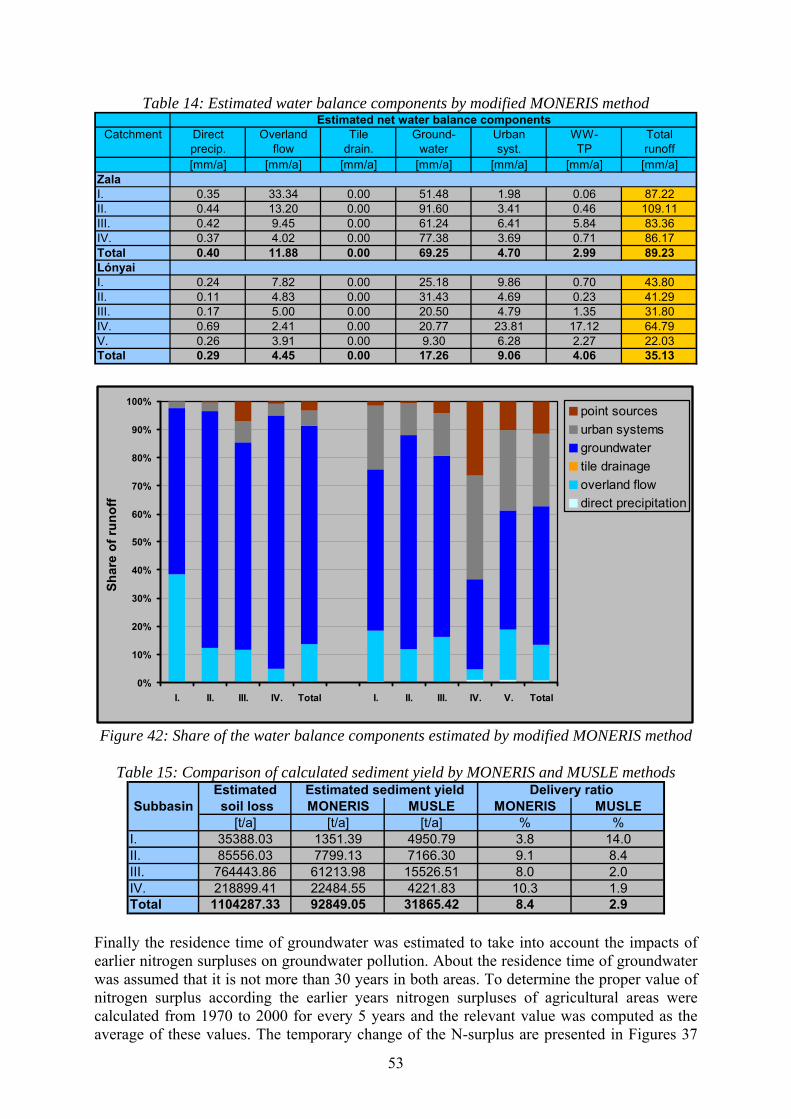
Table 14: Estimated water balance components by modified MONERIS method

Catchment Direct Overland Tile Ground- Urban WW- Totalprecip. flow drain. water syst. TP runoff[mm/a] [mm/a] [mm/a] [mm/a] [mm/a] [mm/a] [mm/a]

ZalaI. 0.35 33.34 0.00 51.48 1.98 0.06 87.22II. 0.44 13.20 0.00 91.60 3.41 0.46 109.11III. 0.42 9.45 0.00 61.24 6.41 5.84 83.36IV. 0.37 4.02 0.00 77.38 3.69 0.71 86.17Total 0.40 11.88 0.00 69.25 4.70 2.99 89.23LónyaiI. 0.24 7.82 0.00 25.18 9.86 0.70 43.80II. 0.11 4.83 0.00 31.43 4.69 0.23 41.29III. 0.17 5.00 0.00 20.50 4.79 1.35 31.80IV. 0.69 2.41 0.00 20.77 23.81 17.12 64.79V. 0.26 3.91 0.00 9.30 6.28 2.27 22.03Total 0.29 4.45 0.00 17.26 9.06 4.06 35.13

Estimated net water balance components

0%

10%

20%

30%

40%

50%

60%

70%

80%

90%

100%

I. II. III. IV. Total I. II. III. IV. V. Total

Shar

e of

runo

ff

point sourcesurban systemsgroundwatertile drainageoverland flowdirect precipitation

Figure 42: Share of the water balance components estimated by modified MONERIS method

Table 15: Comparison of calculated sediment yield by MONERIS and MUSLE methods

EstimatedSubbasin soil loss MONERIS MUSLE MONERIS MUSLE

[t/a] [t/a] [t/a] % %I. 35388.03 1351.39 4950.79 3.8 14.0II. 85556.03 7799.13 7166.30 9.1 8.4III. 764443.86 61213.98 15526.51 8.0 2.0IV. 218899.41 22484.55 4221.83 10.3 1.9Total 1104287.33 92849.05 31865.42 8.4 2.9

Estimated sediment yield Delivery ratio

Finally the residence time of groundwater was estimated to take into account the impacts of earlier nitrogen surpluses on groundwater pollution. About the residence time of groundwater was assumed that it is not more than 30 years in both areas. To determine the proper value of nitrogen surplus according the earlier years nitrogen surpluses of agricultural areas were calculated from 1970 to 2000 for every 5 years and the relevant value was computed as the average of these values. The temporary change of the N-surplus are presented in Figures 37

53

and 39 (see Chapter 5.4). The nitrogen surplus values used to calculate groundwater emissions in the different sub-catchments are shown in Figures 43-44. The differences between the current and the long term average values are significant in all areas. It is caused by the great decrease of fertilizer application in Hungary since the begining of the 1990’s. However, for groundwater system characterization the past higher values seem to be more suitable.

9.7929.56

15.1461.13

14.5055.64

12.1435.88

currentlong term aver.

Figure 43: Current and long term (30 years) average nitrogen surpluses in Zala catchment

8.8549.11

9.4249.24

9.1446.83

14.5551.45

8.6546.73

currentlong term aver.

Figure 44: Current and long term (30 years) average nitrogen surpluses in Lónyai catchment

54

6.2 Results 6.2.1 Original method Tables 16 and 18 and Figures 45-48 show the results of the original method applied in both catchments. Regarding the nitrogen emissions the total emission is from the whole catchment is 621 t/a in Zala watershed. The biggest part of it originates from III Sub-catchment, which is the largest area and it has a significant WWTP. Sub-catchment I contributes to the total basin emission in the lowest degree, because the agricultural land use is here not so intensive. In Lónyai watershed the total amount of emitted nitrogen is 734 t/a. Significant source areas are sub-basin IV and V, which have large WWTP’s without nutrient removal. The others are small regions and they have only small treatment plants. The area-specific emissions are different in the case study areas. In Zala catchment the specific total nitrogen emission from the total area is 4.1 kg/ha/a, but this value is only 3.5 kg/ha/a in Lónyai area. It would be much lower, if emissions of WWTP’s in sub-basin IV were not so significant. The specific values in Zala catchment vary between 2.3 and 4.6 kg/ha/a, but in Lónyai catchment excluding sub-basin IV the values change between 1 and 2 kg/ha/a. However, specific nitrogen emission in sub-basin IV is very large (13.2 kg/ha/a), which result in a higher value for the total watershed. Concerning the share of the different pathways the subsurface sources (groundwater and tile drainage, they have 39 and 16 % proportion, respectively) have the greatest importance in Zala catchment. Beside these erosion and WWTP’s are remarkable (19-18 %), especially in sub-basin III and IV and the total catchment. The dominance of subsurface processes (50-80 %) is valid for all examined areas. Although drained areas have minor importance in the agricultural regions, the nitrogen loss due to the denitrification is less than in groundwater zone with long residence time, so majority of nitrogen surplus in drained agricultural land reaches the surface water. In Zala catchment 82 % of nitrogen emission entering the river system is related to diffuse sources. However, the situation is different in Lónyai catchment. Emissions from point sources have the biggest share on the total emission, especially in sub-catchment IV and V, consequently also in the total watershed (78 %). Non-point pathways have only 22 % proportion in the whole catchment. In Sub-basins I-III the majority of nutrient inputs originate from diffuse sources (50-80 %). Regarding the diffuse sources erosion and urban areas have notable share beside the subsurface processes. Groundwater has surprisingly low contribution to the total emission especially in sub-basin IV and V because of the slight groundwater recharge from the surface and the very intensive predicted denitrification of nitrate in groundwater zone.

Table 16: Calculated nitrogen emissions with the original MONERIS model (for the period 1997-2001)

Catchment Atmospheric Overland Erosion Tile Ground- Urban WWTP Totaldeposition flow drainage water systems emissions

[t/a] [t/a] [t/a] [t/a] [t/a] [t/a] [t/a] [t/a]ZalaI. 0,76 1,44 5,02 12,72 19,29 2,90 0,87 43,00II. 1,25 3,01 15,40 27,79 75,25 3,42 3,08 129,20III. 3,34 5,46 70,32 45,48 96,76 11,85 89,76 322,98IV. 1,41 2,82 28,88 16,16 51,96 3,89 20,39 125,50Total 6,76 12,72 119,63 102,15 243,25 22,07 114,10 620,67LónyaiI. 1,47 0,94 4,25 4,73 8,28 4,55 16,37 40,58II. 0,51 0,64 2,77 2,72 7,05 3,33 4,62 21,63III. 2,13 1,00 6,91 0,20 7,05 7,56 22,45 47,29IV. 3,58 1,91 4,94 12,22 3,55 16,27 395,83 438,30V. 6,68 1,43 15,65 19,60 2,54 8,13 132,51 186,53Total 14,37 5,91 34,52 39,47 28,46 39,84 571,77 734,33

Estimated net nitrogen emissions

55

0

2

4

6

8

10

12

14

I. II. III. IV. Total I. II. III. IV. V. Total

Nitr

ogen

em

issi

on [k

g N

/ha]

WWTP'sUrban systemsGroundwaterTile drainageErosionOverland flowDeposition

LónyaiZala Figure 45: Calculated area-specific nitrogen emissions with the original MONERIS model

(for the period 1997-2001)

0%

10%

20%

30%

40%

50%

60%

70%

80%

90%

100%

I. II. III. IV. Total I. II. III. IV. V. Total

Nitr

ogen

, sha

re o

f pat

hway

[%]

WWTP'sUrban systemsGroundwaterTile drainageErosionOverland flowDeposition

Zala Lónyai Figure 46: Share of different pathways on total nitrogen emission calculated with the original

MONERIS model (for the period 1997-2001)

Table 17 shows the nitrogen emissions summed according to the catchment outlets, where river quality data are available. It is required in the case of Zala watershed only, where the sub-catchments are downstream each other, consequently the sampling points detect the impacts of all upstream sub-catchments. In Lónyai catchment the parts are connected in “parallel” way and only the final sub-basin is upstream the others. But for the final outlets the emissions were once calculated (see Table 16, rows called “Total”).

56

Table 17: Calculated summed nitrogen emissions with the original MONERIS model (for the period 1997-2001)

Catchment Atmospheric Overland Erosion Tile Ground- Urban WWTP Totaldeposition flow drainage water systems emissions

[t/a] [t/a] [t/a] [t/a] [t/a] [t/a] [t/a] [t/a]ZalaI. 0,76 1,44 5,02 12,72 19,29 2,90 0,87 43,00I.+II. 2,02 4,45 20,42 40,51 94,54 6,32 3,94 172,20I. + II. + III. 5,35 9,90 90,74 85,99 191,29 18,18 93,71 495,17I. + II. + II. + IV. 6,76 12,72 119,63 102,15 243,25 22,07 114,10 620,67

Estimated summed nitrogen emissions

Concerning the phosphorus emissions the total emissions from the whole Zala catchment is 187 t/a. Similar to the nitrogen emissions sub-basin III yields the biggest and sub-basin I the lowest phosphorus contamination. The difference is due to the differing amount of eroded soil transported into the river. In Lónyai watershed the total P-emission from the total area is 123 t/a, subbasin IV (WWTP’s) and V (WWTP’s and erosion) contributes to it in the most remarkable degree. The area-specific phosphorus emissions in Zala catchment vary in a wider range (between 0.4 and 1.6 kg/ha), the average for the total area is 1.2 kg/ha. This variation is explainable with the increase of arable land proportion in the watershed area and of the specific soil loss rate. The variation of specific emissions in Lónyai watershed excluding sub-basin IV is not so significant (between 0.3 and 0.6 kg/ha/a), the extreme high value of sub-basin IV (1.6 kg/ha) compared to others in this region is caused by the big WWTP of Nyíregyháza city without phosphorus elimination. But this value affects a higher specific value for the total watershed (0.6 kg/ha/a). Regarding the share of the sources almost the total emission (about 85-90 %) is caused by the erosion in Zala watershed and its sub-basins. Other diffuse sources have minor importance, and point source emissions are also little due to the P-elimination applied at WWTP’s in this region. 95 % of the total emitted phosphorus fluxes originate from non-point sources. Impacts of erosion and WWTP’s dominate in Lónyai catchment, where 56 % of the emissions arise from point sources and the rest from diffuse pathways. In the diffuse pollutions erosion is the most remarkable source, beside this urban systems and groundwater are relative important. In sub-basins with lower point source influence (I-III) the proportion of erosion is more than 40 %. Groundwater has in these cases surprisingly high role in the emissions. However, this is only relative importance due to the low level of the total phosphorus emissions in these areas.

Table 18: Calculated phosphorus emissions with the original MONERIS model (for the period

1997-2001)

Catchment Atmospheric Overland Erosion Tile Ground- Urban WWTP Totaldeposition flow drainage water systems emissions

[t/a] [t/a] [t/a] [t/a] [t/a] [t/a] [t/a] [t/a]ZalaI. 0,03 0,30 6,53 0,19 0,22 0,19 0,16 7,61II. 0,05 0,89 21,23 0,29 0,56 0,29 0,21 23,53III. 0,12 1,56 98,32 0,75 3,27 1,87 5,23 111,12IV. 0,05 0,86 38,25 0,43 1,10 0,42 3,19 44,29Total 0,25 3,60 164,33 1,67 5,15 2,77 8,78 186,55LónyaiI. 0,05 0,32 4,80 0,21 1,30 0,42 2,89 10,01II. 0,02 0,19 3,02 0,13 0,95 0,26 0,82 5,38III. 0,08 0,35 7,47 0,39 1,55 1,18 3,19 14,22IV. 0,13 0,67 5,32 0,38 0,92 2,58 44,07 54,07V. 0,25 0,51 17,76 0,91 1,27 0,85 17,79 39,33Total 0,53 2,04 38,38 2,02 5,99 5,29 68,76 123,00

Estimated net phosphorus emissions

57

0,0

0,2

0,4

0,6

0,8

1,0

1,2

1,4

1,6

1,8

I. II. III. IV. Total I. II. III. IV. V. Total

Phos

phor

us e

mis

sion

[kg

P/ha

]

WWTP'sUrban systemsGroundwaterTile drainageErosionOverland flowDeposition

LónyaiZala Figure 47: Calculated area-specific phosphorus emissions with the original MONERIS model

(for the period 1997-2001)

0%

10%

20%

30%

40%

50%

60%

70%

80%

90%

100%

I. II. III. IV. Total I. II. III. IV. V. Total

Phos

phor

us, s

hare

of p

athw

ay [%

]

WWTP'sUrban systemsGroundwaterTile drainageErosionOverland flowDeposition

Zala Lónyai Figure 48: Share of different pathways on total nitrogen emission calculated with the original

MONERIS model (for the period 1997-2001) Table 19 shows the phosphorus emissions summed according to the catchment outlets, where river quality data are available. It is required in the case of Zala watershed only, where the sub-catchments are downstream each other, consequently the sampling points detect the impacts of all upstream sub-catchments. In Lónyai catchment the parts are connected in “parallel” way and only the final sub-basin is upstream the others. But for the final outlets the emissions were once calculated (see Table 18, rows called “Total”).

58

Table 19: Calculated summed phosphorus emissions with the original MONERIS model (for the period 1997-2001)

Catchment Atmospheric Overland Erosion Tile Ground- Urban WWTP Totaldeposition flow drainage water systems emissions

[t/a] [t/a] [t/a] [t/a] [t/a] [t/a] [t/a] [t/a]ZalaI. 0,03 0,30 6,53 0,19 0,22 0,19 0,16 7,61I.+II. 0,07 1,19 27,76 0,49 0,78 0,48 0,37 31,14I. + II. + III. 0,20 2,75 126,08 1,24 4,05 2,35 5,59 142,26I. + II. + II. + IV. 0,25 3,60 164,33 1,67 5,15 2,77 8,78 186,55

Estimated summed phosphorus emissions

6.2.2 Modified method Tables 20 and 22 and Figures 49-52 present the results of the modified version of MONERIS. The total nitrogen emissions of the whole Zala catchment is in this case significantly less then before: it is 516 t/a. The difference is obviously due to the lack of drainage systems and to the modification of water balance and erosion calculations. Emission via drainage systems was transported to groundwater flow only partly, because the retention in groundwater is much higher than in the case of drain-flow. Consequently groundwater emission was increased, but the total nitrogen flux was decreased. Additionally nitrogen emission via erosion was decreased due to the calculated less sediment input. Finally the impact of overland flow was intensified because surface runoff amount is higher in this version. The fluxes from other sources are unvarying. In Lónyai catchment the alterations affect the subsurface components and the overland flow (erosion was not modified). Since nitrogen emissions from tile drainage were not too much and the calculated denitrification rate is quite high, the total N-emission was decreased and N-fluxes via groundwater were increased in minor degree than in Zala catchment (total emission is 711 t/a). Additionally overland flow related emissions were also increased. The spatial differences among the sub-basins are similar than in the original calculations. Regarding the area-specific values they decreased significantly in Zala watershed (they move between 2 and 4 kg/ha/a, the average is 3.4 kg/ha/a). In Lónyai catchment the changes are not numerous, the values are similar to the original version. The share of the different pathways was also varied naturally. In Zala catchment groundwater is the most important source with 53 % proportion on the total emissions. Surface processes (erosion and overland flow) are less relevant (erosion: 14 %, overland flow: 6 %), however, for example in sub-basin I these processes have more than 50 % share, which is due to the higher surface runoff amount (upper part of the watershed). Point sources provide the 22 % of the total nitrogen fluxes, so majority of nitrogen input is originated from non-point sources. In Lónyai catchment the ratio between non-point / point sources is reverse: only 20 % of the emissions is related to diffuse sources, while 80 % of the emissions is released by point sources. In sub-basins with smaller point sources (I-III) similarly to the original method the diffuse pollutions have 55-75 % share. But there are not an obviously dominant diffuse source as it was the groundwater in Zala catchment. In Lónyai watershed erosion, overland flow and urban areas have also remarkable impact, beside the groundwater.

59

Table 20: Calculated nitrogen emissions with the modified MONERIS model (for the period 1997-2001)

Catchment Atmospheric Overland Erosion Tile Ground- Urban WWTP Totaldeposition flow drainage water systems emissions

[t/a] [t/a] [t/a] [t/a] [t/a] [t/a] [t/a] [t/a]ZalaI. 0,76 10,09 9,99 0,00 13,26 2,90 0,87 37,88II. 1,25 6,35 14,72 0,00 85,72 3,42 3,08 114,55III. 3,34 11,62 33,99 0,00 110,57 11,85 89,76 261,13IV. 1,41 2,43 11,90 0,00 62,33 3,89 20,39 102,36Total 6,76 30,50 70,61 0,00 271,89 22,07 114,10 515,92LónyaiI. 1,47 3,70 4,25 0,00 7,26 4,55 16,37 37,60II. 0,51 1,65 2,77 0,00 7,21 3,33 4,62 20,08III. 2,13 3,73 6,91 0,00 7,72 7,56 22,45 50,50IV. 3,58 1,47 4,94 0,00 7,00 16,27 395,83 429,09V. 6,68 6,60 15,65 0,00 4,04 8,13 132,51 173,61Total 14,37 17,16 34,52 0,00 33,23 39,84 571,77 710,88

Estimated net nitrogen emissions

0

2

4

6

8

10

12

14

I. II. III. IV. Total I. II. III. IV. V. Total

Nitr

ogen

em

issi

on [k

g N

/ha]

WWTP'sUrban systemsGroundwaterTile drainageErosionOverland flowDeposition

LónyaiZala Figure 49: Calculated area-specific nitrogen emissions with the modified MONERIS model

(for the period 1997-2001)

60

0%

10%

20%

30%

40%

50%

60%

70%

80%

90%

100%

I. II. III. IV. I. II. III. IV. V.

Nitr

ogen

, sha

re o

f pat

hway

[%]

WWTP'sUrban systemsGroundwaterTile drainageErosionOverland flowDeposition

Zala Lónyai Figure 50: Share of different pathways on total nitrogen emission calculated with the

modified MONERIS model (for the period 1997-2001)

Table 21 shows the nitrogen emissions summed according to the catchment outlets, where river quality data are available. It is required in the case of Zala watershed only, where the sub-catchments are downstream each other, consequently the sampling points detect the impacts of all upstream sub-catchments. In Lónyai catchment the parts are connected in “parallel” way and only the final sub-basin is upstream the others. But for the final outlets the emissions were once calculated (see Table 20, rows called “Total”). Table 21: Calculated summed nitrogen emissions with the modified MONERIS model (for the

period 1997-2001)

Catchment Atmospheric Overland Erosion Tile Ground- Urban WWTP Totaldeposition flow drainage water systems emissions

[t/a] [t/a] [t/a] [t/a] [t/a] [t/a] [t/a] [t/a]ZalaI. 0,76 10,09 9,99 0,00 13,26 2,90 0,87 37,88I.+II. 2,02 16,45 24,71 0,00 98,99 6,32 3,94 152,44I. + II. + III. 5,35 28,06 58,70 0,00 209,56 18,18 93,71 413,56I. + II. + II. + IV. 6,76 30,50 70,61 0,00 271,89 22,07 114,10 515,92

Estimated summed nitrogen emissions

Concerning the phosphorus emissions of Zala catchment the total emission (123 t/a) is reduced due to the change in the calculated sediment load volume. Neglecting of tile drainage and changes in water balance has minor importance on the emission values because of the small P-concentrations in subsurface water (only P-input via overland flow was increased). Emissions in Lónyai watershed did not change remarkable (126 t/a), only the impact of overland flow became more intensive, but only relatively. Spatial differences in emissions among the sub-basins are similar to the original results. Examining the area-specific values, they varied in Zala catchment significantly. The value for total catchment was decreased (0.80 kg/ha) and the intensive fluctuation of sub-basin emissions became much more moderate than before (they vary between 0.6 and 0.9 kg/ha). In Lónyai catchment the specific emissions are similar to the first results. Share of non-point sources is about 93 % in total Zala watershed, however emissions from the two upper sub-basin are almost completely diffuse pollutions. Erosion has an obvious dominance (80 %), overland flow and groundwater have the rest. Regarding Lónyai watershed 55 % of total pollutions originate from point sources. About 30

61

% is the share of erosion. Overland flow, groundwater and urban areas are less notable. In sub-basins with smaller WWTP’s (I-III) the share of erosion is 45-50 %.

Table 22: Calculated phosphorus emissions with the modified MONERIS model (for the

period 1997-2001)

Catchment Atmospheric Overland Erosion Tile Ground- Urban WWTP Totaldeposition flow drainage water systems emissions

[t/a] [t/a] [t/a] [t/a] [t/a] [t/a] [t/a] [t/a]ZalaI. 0,03 2,13 12,99 0,00 0,47 0,19 0,16 15,96II. 0,05 1,87 20,30 0,00 0,65 0,29 0,21 23,37III. 0,12 3,31 47,52 0,00 3,71 1,87 5,23 61,77IV. 0,05 0,74 15,76 0,00 1,28 0,42 3,19 21,44Total 0,25 8,06 96,57 0,00 6,11 2,77 8,78 122,54LónyaiI. 0,05 1,26 4,80 0,00 1,23 0,42 2,89 10,66II. 0,02 0,50 3,02 0,00 0,98 0,26 0,82 5,59III. 0,08 1,31 7,47 0,00 1,66 1,18 3,19 14,90IV. 0,13 0,51 5,32 0,00 1,35 2,58 44,07 53,97V. 0,25 2,37 17,76 0,00 1,66 0,85 17,79 40,67Total 0,53 5,95 38,38 0,00 6,89 5,29 68,76 125,79

Estimated net phosphorus emissions

0,0

0,2

0,4

0,6

0,8

1,0

1,2

1,4

1,6

1,8

I. II. III. IV. Total I. II. III. IV. V. Total

Phos

phor

us e

mis

sion

[kg

P/ha

]

WWTP'sUrban systemsGroundwaterTile drainageErosionOverland flowDeposition

LónyaiZala Figure 51: Calculated area-specific phosphorus emissions with the modified MONERIS

model (for the period 1997-2001)

62

0%

10%

20%

30%

40%

50%

60%

70%

80%

90%

100%

I. II. III. IV. I. II. III. IV. V.

Phos

phor

us, s

hare

of p

athw

ay [%

]

WWTP'sUrban systemsGroundwaterTile drainageErosionOverland flowDeposition

Zala Lónyai Figure 52: Share of different pathways on total phosphorus emission calculated with the

modified MONERIS model (for the period 1997-2001) Table 23 shows the phosphorus emissions summed according to the catchment outlets, where river quality data are available. It is required in the case of Zala watershed only, where the sub-catchments are downstream each other, consequently the sampling points detect the impacts of all upstream sub-catchments. In Lónyai catchment the parts are connected in “parallel” way and only the final sub-basin is upstream the others. But for the final outlets the emissions were once calculated (see Table 22, rows called “Total”). Table 23: Calculated summed phosphorus emissions with the modified MONERIS model (for

the period 1997-2001)

Catchment Atmospheric Overland Erosion Tile Ground- Urban WWTP Totaldeposition flow drainage water systems emissions

[t/a] [t/a] [t/a] [t/a] [t/a] [t/a] [t/a] [t/a]ZalaI. 0,03 2,13 12,99 0,00 0,47 0,19 0,16 15,96I.+II. 0,07 4,00 33,29 0,00 1,12 0,48 0,37 39,33I. + II. + III. 0,20 7,32 80,81 0,00 4,83 2,35 5,59 101,10I. + II. + II. + IV. 0,25 8,06 96,57 0,00 6,11 2,77 8,78 122,54

Estimated summed phosphorus emissions

Another possibility to assess the nutrient emissions is examination of impacts of different activities on the total emissions. Emissions from the natural background, agriculture, waste water management (including rainfall) and combustion processes were selected as activities. Atmospheric deposition was divided into natural background and combustion part. A certain amount of erosion was considered as natural sediment input from the watershed. Additionally a natural background phosphorus concentration was assumed in overland flow and groundwater. Based on these assumptions were the background and the combustion emissions calculated. Additionally waste water emissions were calculated as the sum of nutrient fluxes from urban systems and point sources. The remained amount of nutrient inputs are presented as agricultural fluxes. Tables 24-25, and Figures 53-54 show the results of this examination (with modified MONERIS). Relatively high amount of background nitrogen emission was found in Zala catchment (24 %). Agriculture has the dominant role (32 %), waste water has a share of 26 % on the total emissions. In sub-basin I background and combustion emissions

63

have bigger importance. In sub-basin II agriculture, in sub-basin III waste water is more intensive. In Lónyai catchment waste water is the dominant activity with 86 % share on the total emissions. Agriculture has only a small role (7 %). However, in sub-basins I-III, where only smaller WWTP’s are located, both agriculture and background are more remarkable. Regarding phosphorus emissions majority of the emissions (87 %) is related to the agriculture in Zala watershed. Share of waste water is 9 %. This value is less in sub-basins I and II, but more in sub-basin IV. Background emission is not significant. In Lónyai watershed the dominant activity in pollution’s point of view is waste water (about 60 %). The rest is originated primarily from agriculture. However, in sub-basins, excluding No. IV, agriculture provides the highest amount of phosphorus pollution. Share of background emission is 5 %, but in sub-basins I-III it varies between 5 and 10 %.

Table 24: Calculated nitrogen emissions related to activities with the modified MONERIS model (for the period 1997-2001)

Catchment Background Agriculture Waste water Combustion Total[kg/ha/a] [kg/ha/a] [kg/ha/a] [kg/ha/a] [kg/ha/a]

ZalaI. 0,71 0,59 0,20 0,51 2,01II. 1,13 1,85 0,23 0,84 4,05III. 0,67 1,06 1,42 0,49 3,64IV. 0,88 0,76 0,71 0,65 3,00Total 0,81 1,08 0,89 0,59 3,38LónyaiI. 0,21 0,29 0,80 0,14 1,44II. 0,21 0,29 0,41 0,14 1,05III. 0,16 0,25 0,74 0,10 1,24IV. 0,17 0,23 12,37 0,11 12,88V. 0,12 0,18 1,54 0,06 1,90Total 0,15 0,22 2,90 0,09 3,37

Estimated net nitrogen emissions

0%

10%

20%

30%

40%

50%

60%

70%

80%

90%

100%

I. II. III. IV. Total I. II. III. IV. V. Total

Nitr

ogen

, sha

re o

f pat

hway

[%]

CombustionWaste waterAgricultureBackground

Zala Lónyai Figure 53: Share of different activities on total nitrogen emission calculated with the modified

MONERIS model (for the period 1997-2001)

64

Table 25: Calculated phosphorus emissions related to activities with the modified MONERIS model (for the period 1997-2001)

Catchment Background Agriculture Waste water Combustion Total[kg/ha/a] [kg/ha/a] [kg/ha/a] [kg/ha/a] [kg/ha/a]

ZalaI. 0,03 0,80 0,02 0,00 0,85II. 0,04 0,77 0,02 0,00 0,83III. 0,03 0,73 0,10 0,00 0,86IV. 0,04 0,49 0,11 0,00 0,63Total 0,03 0,69 0,08 0,00 0,80LónyaiI. 0,03 0,25 0,13 0,00 0,41II. 0,03 0,20 0,06 0,00 0,29III. 0,03 0,23 0,11 0,00 0,37IV. 0,03 0,19 1,40 0,00 1,62V. 0,03 0,21 0,20 0,00 0,44Total 0,03 0,22 0,35 0,00 0,60

Estimated net phosphorus emissions

0%

20%

40%

60%

80%

100%

I. II. III. IV. Total I. II. III. IV.

Phos

phor

us, s

hare

of p

athw

ay [%

]

CombustionWaste waterAgricultureBackground

Zala Lónyai Figure 54: Share of different activities on total phosphorus emission calculated with the

modified MONERIS model (for the period 1997-2001)

7. COMPARISON OF RESULTS WITH THE MEASURMENTS 7.1 River loads and nutrient retentions The calculated nutrient emissions can be compared with the measured river loads at the catchment outlet if river retention processes are taken into account. Using the river retention model of MONERIS the calculated DIN-, TN- and TP loads were checked at 3 monitoring points in Zala watershed and at two points in Lónyai catchment. Both of DIN- and TP-loads were calculated based on specific runoff and hydraulic loads of the catchments. Additionally TN-loads were calculated also based on hydraulic load (with different model parameters) and TP-loads were calculated as a result following the average value of retention parameter based on specific runoff (SR) and hydraulic load (HL). During

65

the comparison the calculated load values based on the ratio method were used as measured river loads. Since measured TN loads in Lónyai catchment were available only for the last year of the 5 years long period, therefore annual river load for this period could not be calculated in the way presented in chapter 5.1. Consequently the share of TN and DIN yearly average loads was computed for the one year when both data exist. Afterwards the DIN load according to the 5 years long period was multiplied with the determined TN/DIN share. The estimated TN river loads of Lónyai catchment can be found in Table 26. Tables 26-27 and Figures 55-65 show the results of river load calculations based on the modified MONERIS approach. There are remarkable differences between SR- and HL-based river load in Zala watershed. In case of DIN, HL-loads are twice greater than SR-loads. For phosphorus the difference is three times. In Lónyai catchment the deviations are significant at Nyírpazony station and at the final outlet (N: 2-3,. P: 4-6 times differences). The situation is very interesting regarding the calculated loads based on SR at the final outlet (Buj-Kótaj). In comparison to Szarvassziget there is a decline in both DIN and TP loads, though the watershed area between the two outlets increases six times. That means the estimated phosphorus inputs from the watershed between the monitoring stations are less than the calculated retention in the river system, i.e. the retention in the river is very intensive. However, in the case of HL, the values are significantly higher at Buj-Kótaj than at Szarvassziget. The calculated TN loads are 10 % greater than the DIN-loads in Zala catchment. In Lónyai catchment the differences are between 50 and 100 %. Concerning the “average” phosphorus loads their values are nearer the SR-loads than the HL-loads due to the non-linear relationship between emissions and loads. The calculated loads fit quite well with the measured loads. For DIN loads the SR-method gives modearately good results: the loads are underestimated at all points, the differences are between 30 and 50 % (excluding the final outlet of Lónyai, where the deviation is 58 %). For TP the SR-approach is acceptable in Zala watershed only. In Lónyai catchment the result are out of the prediction limit and the deviations are too great. HL-calculations for DIN overestimate the registred loads (excluding Zalaegerszeg and Szarvassziget station), the differences are acceptable (less than or near 20 %). Calculation of TP-loads based on HL has poor results, the differences especially in Zala catchment are too high. However, the results for Lónyai watershed are better than the SR-values. For Zala catchment SR-method provides more proper results. TN loads based on HL fit quite well with the measured loads, even the greatest diffreence is lower than 50 %. TP-load calculation using SR and HL as average gives good results for Zala watershed, however it underestimates the loads for Lónyai watershed.

Table 26: Calculated nutrient river loads based on the emissions of modified MONERIS model (for the period 1997-2001)

Catchmentoutlet TN TP DIN load TP load DIN load TP load TN load TP load DIN TN TP

hydr. load average[t/a] [t/a] [t/a] [t/a] [t/a] [t/a] [t/a] [t/a] [t/a] [t/a] [t/a]

ZalaZalalövő 37,88 15,96 11,64 2,81 23,85 9,05 26,65 4,29 no data no data no dataZalaegerszeg 152,44 39,33 52,01 8,41 98,23 23,08 108,57 12,33 103,45 166,35 13,53Zalabér 413,56 101,10 130,28 18,66 255,01 55,65 287,84 27,95 219,31 346,80 26,35Zalaapáti 515,92 122,54 161,33 22,31 318,99 67,72 359,58 33,56 271,51 429,68 34,75LónyaiLaskod 37,60 10,66 6,47 0,66 7,15 1,08 14,83 0,82 no data no data no dataLevelek 20,08 5,59 3,28 0,31 3,24 0,45 7,30 0,37 no data no data no dataNyírpazony 50,50 14,90 6,44 0,55 12,33 2,13 22,48 0,87 no data no data no dataSzarvassziget 429,09 53,97 104,02 6,16 115,68 8,90 200,26 7,28 148,12 160,98 36,49Buj-Kótaj 710,88 125,79 99,73 5,44 275,04 34,89 393,86 9,41 239,77 262,30 54,33

Estimated nutrient river loadsMeasured loads

specific runoff hydraulic load

Nutrient emissionsSummed

emissions

Calculated

66

Table 27: Differences between the calculated and measured river loads based on the

emissions of modified MONERIS model (for the period 1997-2001)

Catchment DIN load TP load DIN load TP load TN load TP loadoutlet hydraulic load average

[%] [%] [%] [%] [%] [%]ZalaZalaegerszeg -49,73 -37,82 -5,05 70,50 -34,74 -8,88Zalabér -40,59 -29,19 16,28 111,18 -17,00 6,06Zalaapáti -40,58 -35,80 17,49 94,88 -16,31 -3,41LónyaiSzarvassziget -29,77 -83,13 -21,90 -75,62 24,39 -80,06Buj-Kótaj -58,41 -89,99 14,71 -35,79 50,16 -82,68

Difference from the measured river loads

specific runoff hydraulic load

0,00

0,25

0,50

0,75

1,00

1,25

1 10

Specific runoff [l/(s˙km2)]

DIN

-load

/TN

-em

issi

on

100

Zala riverLónyai riverRetention model90 % prediction level

Figure 55: Ratio between measured and modeled DIN load and TN emission calculated with the modified MONERIS model in dependence on specific runoff (for the period 1997-2001)

67

0

1

2

3

4

5

0 1 2 3 4 5

Measured DIN load [kg/ha/a]

Cal

cula

ted

DIN

load

[kg/

ha/a

]

1:1 line+/- 30 % deviationZala riverLónyai river

Specific runoff

Figure 56: Comparison of measured and modeled DIN load calculated based on the modified

MONERIS model in dependence on specific runoff (for the period 1997-2001)

0,00

0,25

0,50

0,75

1,00

1,25

1 10Specific runoff [l/(s˙km2)]

TP-lo

ad/T

P-em

issi

on

100

Zala riverLónyai riverRetention model90 % prediction level

Figure57: Ratio between measured and modeled TP load and TP emission calculated with the

modified MONERIS model in dependence on specific runoff (for the period 1997-2001)

68

0

0,2

0,4

0,6

0,8

1

0,0 0,2 0,4 0,6 0,8 1,0 1,2

Measured TP load [kg/ha/a]

Cal

cula

ted

TP lo

ad [k

g/ha

/a]

1:1 line+/- 30 % deviationZala riverLónyai river

Specific runoff

Figure 58: Comparison of measured and modeled TP load calculated based on the modified

MONERIS model in dependence on specific runoff (for the period 1997-2001)

0,00

0,25

0,50

0,75

1,00

1,25

1 10 100 1000

Hydraulic load [m/a]

DIN

-load

/TN

-em

issi

on

Zala riverLónyai riverRetention model90 % prediction level

Figure 59: Ratio between measured and modeled DIN load and TN emission calculated with the modified MONERIS model in dependence on hydraulic load (for the period 1997-2001)

69

0

1

2

3

4

5

0 1 2 3 4 5

Measured DIN load [kg/ha/a]

Cal

cula

ted

DIN

load

[kg/

ha/a

]

1:1 line+/- 30 % deviationZala riverLónyai river

Hydraulic load

Figure 60: Comparison of measured and modeled DIN load calculated based on the modified

MONERIS model in dependence on hydraulic load (for the period 1997-2001)

0,00

0,25

0,50

0,75

1,00

1,25

1 10 100 1000

Hydraulic load [m/a]

TP-lo

ad/T

P-em

issi

on

Zala riverLónyai riverRetention model90 % prediction level

Figure 61: Ratio between measured and modeled TP load and TP emission calculated with the modified MONERIS model in dependence on hydraulic load (for the period 1997-2001)

70

0

0,2

0,4

0,6

0,8

1

0 0 0 1 1 1

Measured TP load [kg/ha/a]

Cal

cula

ted

TP lo

ad [k

g/ha

/a]

1

1:1 line+/- 30 % deviationZala riverLónyai river

Hydraulic load

Figure 62: Comparison of measured and modeled TP load calculated based on the modified

MONERIS model in dependence on hydraulic load (for the period 1997-2001)

0,00

0,25

0,50

0,75

1,00

1,25

0 1 10 100 1000

Hydraulic load [m/a]

TN-lo

ad/T

N-e

mis

sion

Zala riverLónyai riverRetention model90 % prediction level

Figure 63: Ratio between measured and modeled TN load and TN emission calculated with the modified MONERIS model in dependence on hydraulic load (for the period 1997-2001)

71

0

1

2

3

4

5

6

7

0 1 2 3 4 5 6

Measured TN load [kg/ha/a]

Cal

cula

ted

TN lo

ad [k

g/ha

/a]

7

1:1 line+/- 30 % deviationZala riverLónyai river

Hydraulic load

Figure 64: Comparison of measured and modeled TN load calculated based on the modified

MONERIS model in dependence on hydraulic load (for the period 1997-2001)

0

0,2

0,4

0,6

0,8

1

0,0 0,2 0,4 0,6 0,8 1,0 1,2

Measured TP load [kg/ha/a]

Cal

cula

ted

TP lo

ad [k

g/ha

/a]

1:1 line+/- 30 % deviationZala riverLónyai river

Specific runoff andhydraulic load average

Figure 65: Comparison of measured and modeled TP load calculated based on the modified MONERIS model in dependence on specific runoff and hydraulic load (for the period 1997-

2001) The estimated emissions can be compared additionally to the separated basic and event load fractions (see Chapter 5.1). To this comparison the different sources of MONERIS were ordered into „basic“ and „event“ pathways. The group of basic sources includes point sources, groundwater, atmospheric deposition (on water surfaces only) and partially urban areas (soil pollution only). The part of event emissions contains overland flow, erosion, tile drainage and partially urban areas (surface runoff only). Here also the the results of the ratio method were used as actual total measured loads, however the proportions of event and basic loads determined based on results of correlation method were also applied (see Table 7). Tables 28 and 29 show the results of the comparisons (based on modified MONERIS results). For

72

nitrogen the results are quite similar for both catchments (there is significant deviation only at Zalaegerszeg outlet, where the share of basic emissions is too high compared to the proportion of basic loads.). For phosphorus the situation is more problematic: in Lónyai catchment the values are similar, but in Zala watershed the estimated event emissions have much higher proportion than event loads, the 45-55 % proportions of event river loads are probable underestimated values. The difference might be due to the inaccuracies in two factors: (i) the correlation to estimate daily load values is inaccurate and (ii) the extension of correlation for basic loads to the range of high flow values is imprecise.

Table 28: Comparison of share of basic and event nitrogen emissions and loads (for the period 1997-2001)

Samplingpoints Basic Event Total Basic Event Total Basic Event Total Basic Event Total

[t/a] [t/a] [t/a] [%] [%] [%] [t/a] [t/a] [t/a] [%] [%] [%]ZalaZalaegerszeg 110,54 41,90 152,44 72,5 27,5 100,0 96,82 69,53 166,35 58,2 41,8 100,0Zalabér 316,54 97,02 413,56 76,5 23,5 100,0 268,59 78,21 346,80 77,4 22,6 100,0Zalaapáti 403,14 112,79 515,92 78,1 21,9 100,0 329,90 97,72 427,62 77,1 22,9 100,0LónyaiSzarvassziget 409,55 19,54 429,09 95,4 4,6 100,0 140,91 20,08 160,98 87,5 12,5 100,0Buj-Kótaj 636,45 74,43 710,88 89,5 10,5 100,0 220,39 41,91 262,30 84,0 16,0 100,0

Estimated nitrogen emission fractions Measured nitrogen load fractions

Table 29: Comparison of share of basic and event phosphorus emissions and loads (for the period 1997-2001)

Samplingpoints Basic Event Total Basic Event Total Basic Event Total Basic Event Total

[t/a] [t/a] [t/a] [%] [%] [%] [t/a] [t/a] [t/a] [%] [%] [%]ZalaZalaegerszeg 1,91 37,42 39,33 4,8 95,2 100,0 6,88 6,66 13,53 50,8 49,2 100,0Zalabér 11,14 89,95 101,10 11,0 89,0 100,0 11,82 14,53 26,35 44,8 55,2 100,0Zalaapáti 15,83 106,71 122,54 12,9 87,1 100,0 17,37 14,24 31,60 54,9 45,1 100,0LónyaiSzarvassziget 45,80 8,17 53,97 84,9 15,1 100,0 32,03 4,46 36,49 87,8 12,2 100,0Buj-Kótaj 77,42 48,37 125,79 61,5 38,5 100,0 36,76 17,58 54,33 67,7 32,3 100,0

Estimated phosphorus emission fractions Measured phosphorus load fractions

Figure 66 shows different area specific nitrogen amounts according to the examined sampling points and to their catchment areas like (i) long-term total nitrogen surplus of the soil, (ii) the calculated nitrogen emission of the river net via groundwater, (iii) the simulated and (iv) the measured nitrogen river loads generated by the groundwater emission. The values of N-surplus and nitrogen emission via groundwater contains the impacts of both agricultural and urban areas. It clearly seems that soil denitrification has the primarily impact on the appearing nitrogen fluxes in the river. Denitrification in the river has less significant contribution to the total nitrogen retention in the catchment system. It decreases the emitted nitrogen mass in lower degree only. The modeled and from measurements calculated values for groundwater river loads fit quite well.

73

0

2

4

6

8

10

Zalaegerszeg Zalabér Zalaapáti Szarvassziget Buj-Kótaj

Are

a sp

ecifi

c N

mas

s [k

g N

/ha]

Long term N surp. of soilN emission via gw.Sim. N river load via gw.Meas. N river load via gw.

34 36 34 3940

Soil N retention River N retention

Total retention

Figure 66: Nitrogen retention in the soil and the river

74

LITERATURE

Arnold, J. et al. (2000): Soil and Water Assessment Tools. Theoretical documentation. Agricultural Research Service, Temple, Texas, The U.S.A.

Behrendt, H. et al. (2000): Modeling of Nutrient Emissions into the River Systems.

Theoretical documentation. Institute of freshwater Ecology and Inland Fisheries, Berlin, Germany.

Behrendt, H. et al. (2003):Harmonised Inventory of Point and Diffuse Emissions of Nitrogen

and Phosphorus for a Transboundary River Basin. Final version of the delivery 5.5 of daNUbs

Bozó, L. (2003): Atmospheric N deposition in the surroundings of Lake Balaton (in

Hungarian). Manuscript, OMSZ, Budapest. daNUbs (2003) deliverable D1.1 - Water balance calculations fort he case study regions

inAustria, Hungary and Romania, Instiute of Hydraulics, Hydrology and Water Resources Management Vienna University of Technology, Department of Sanitary and Environmental Engineering Budapest University of Technology, Department of System Ecology and Sustainable Development University of Bucharest

daNUbs (2003) deliverable D2.1 – Evaluated model on estimating nutrient flows due to

erosion/runoff in the case study areas selected Institute for Land and Water Management Research, Federal Agency for Water Management, Petzenkirchen Department of Sanitary and Environmental Engineering Technical Budapest University of Technology and Economics

Fastenau, F. A., van der Graaf, H. J. M., Martijnse, G. (1990): Comparison of various system

for onsite wastewater treatment. Water Science and Technology, 22 (3-4): 41-48. Knowles (1982): Denitrification. Microbiological Reviews, 3: 43-70. Nitrates Directive (91/676/EEC): Water pollution caused by Nitrates from agricultural sources Reneau, R.B., J.J. Simon, M.J. Degen (1985): Treatment By onsite system. Utilization,

Treatment, amd Disposal of Waste on Land. Soil Science Society of America, Inc. Madison, Wisconsin, USA

Schwarze, R. et al. (2000): Difference Time Series Analysis Method. Theoretical

documentation. Institution of Hydrology and Meteorology, University of Technology, Dresden, Germany.

Tombor, S. K. and Simonffy, Z. (2004): Impact of polluted groundwater under the settlements

on the water quality of small watercourses. Manuscript. Budapest University of Technology and Economics, Budapest.

75

DEPARTM AND EN

ENINS

DE

COMPARISON OFINVESTIGATION

FACTORS INFLUEN

VIENNA UNIVERSITY OF TECHNOLOGY

TITUTE FOR WATER QUALITY AND WASTE MANAGEMENT

BUTE ENT OF SANITARYVIRONMENTAL

GINEERING

Part III

LIVERABLE D 1.4

RESULTS FROM S AND EVALUATICING THE NUTR

UNIVERSITY OF BUCHARESTDEPARTMENT OF SYSTEMS

ECOLOGY AND SUSTAINABLEDEVELOPMENT

CASE STUDY ON OF KEY IENT FLUXES

Table of Content

1. Introduction 2

2. Differences in characteristics of the case study regions 2

3. Dominance of CSR in comparison with the Danube catchments 7

4. Nitrogen and phosphorus surpluses on soils 16

5. Influence of discharge conditions on N and P loads 18

6. Possibilities for estimating point source emissions 25

6.1. Materials and Methods 26

6.2. Development of standard values 26

6.3. Validation of Estimations Based on Standard Values 30

6.4. Conclusions 32

7. Emission calculation using MONERIS 32

8. River loads and retention in surface waters 38

9. Evaluation of key parameters and conclusion 42

9.1. Nitrogen 42

9.2. Phosphorus 46

10. References 49

1

1. Introduction The main goal of this deliverable D1.4 is the comparison of the results from the 5 case study regions. This is done based on the reports of the different case study regions from Deliverable D1.3. The results are summarised and presented in respect to similarities and differences between the case study regions in terms of factors influencing nutrient fluxes. To show the relevance of this investigations for Basin wide nutrient balance calculations the main natural and anthropogenic characteristics of the case study areas (CSA) are compared with the distribution of regional characterisation over the whole Danube Basin. In respect to evaluation of key parameters influencing nutrient fluxes on catchment scale and conclusions the findings of the reports of the different countries on the nutrient balances in case study regions are included. The results of deliverable D1.3 are only repeated here as far as this is necessary for comparison between the different catchments.

2. Main differences in characteristics of the case study regions Under the premise of investigations on the case study level primarily 6 case study regions were selected, which should represent the different conditions the Danube Basin is covering. The location is shown in Figure 1. This Deliverable D1.4 presents results from 5 of the 6 case study areas (Ybbs and Wulka (Austria), Zala and Lonyai (Hungary) and Neajlov (Romania)). For the case study region Lesnovska (Bulgaria) no data were obtained in respect to the nutrient balance calculations. Thus, this deliverable will concentrate on the presentation and the comparison of the results which were obtained for the remaining 5 case study areas.

Figure 1: Overview on the location of the 6 primarily selected case study areas

With reference to Deliverable D1.3 not all of the main characteristics will be discussed here. Aim of this chapter is to point out differences in the hydrological and geological conditions as well as in landuse management which are of a major influence on calculated nutrient

2

balances. The most important characteristics of the 5 case study regions (CSA) are presented in Table 1. Table 1: Comparison of main characteristics of the 5 case study regions (1996-2001)

Country RomaniaName of the river Ybbs Wulka Zala Lonyai NeajolovTotal catchment area km2 1105 383 1529 2151 3679share of arable land % 12 54 54 76 78share of agricultural grassland % 27 12 8 4 4share of forests % 52 28 34 14 10N-fertiliser application* kg/haAA/a 150 100 47 25 69P-fertiliser application* kg/haAA/a 43 26 9 5 15N-surplus in agriculture kg/haAA/a 73 50 3 (14***) (-16) (10***) 28P-surplus in agriculture kg/haAA/a 25 17 0.2 (1.5***) (-3) (0.2***) 6N-in agricultural soil g/kg 3.6 1.5 1.2 0.9 1.6P-in agricultural soil g/kg 0.8 0.7 0.7 0.4 0.5N-deposition kg/ha/a 19 13.5 10 10 11average N-surplus on total area kg/ha/a 40 38 12*** 10*** 25average P-surplus on total area kg/ha/a 10 11 1.1*** 0.3*** 5mean slope % 30 8 6.3 0.9 0.22average precipitation mm/a 1390 665 651 629 500average runoff** mm/a 930 99 89 35 72share of point source contribution % 0.7 26 3.3 11.6 2.6population density inh/km2 68 133 79 147 57share conneceted to sewerage % 74 95 50 41 6share conneceted to wwtp % 74 95 50 41 6predominant waste water treatment C, N, (D), P C, N, D, P C, N(D), P C, N 0, C

area specific N load from wwtp kg/ha/a 0.93 1.11 0.75 2.66 0.34area specific P load from wwtp kg/ha/a 0.12 0.09 0.06 0.32 0.025area specific river loads N (TN) kg/ha/a 19 5 2.81 1.24 (DIN) 2.63area specific river loads P (TP) kg/ha/a 0.8 0.3 0.23 0.26 0.13* total application of fertilzer (incl. org., min., sewage sludge) related to agricultural area (haAA)in use **without contribution from point sources*** with consideration of net-mineralization

Austria Hungary

Hydrological conditions

In Table 1 the main hydrological statistics are shown. The average annual amount of precipitation ranges between 1390 mm (Ybbs) and 500 mm (Neajlov. Except Ybbs all other CSAs are below 665mm. Between the two Austrian case study regions Ybbs and Wulka there is a quite big difference of 725 mm/a. More details on the hydrology of the regions can be found in D 1.1 (water balance calculations). These hydrological conditions are reflected in the annual river discharges. However, the discharge in Neajlov is higher than the one in Lonyai. Figure 2 shows the comparison of the river discharges between the case study regions with additional information about the measured average TN and TP concentrations in the river.

3

0

200

400

600

800

1000

Ybbs Wulka Zala Lónyai Neajlov

river

dis

char

ge

0

2

4

6

8

10

TN c

once

ntra

tions

discharge [mm/a]concentration [mg/l]

0

200

400

600

800

1000

Ybbs Wulka Zala Lónyai Neajlov

disc

harg

e

0.0

0.2

0.4

0.6

0.8

1.0

TP c

once

ntra

tions

discharge [mm/a]concentration [mg/l]

Figure 2: Annual river discharges in comparison with measured average TN and TP concentrations in the rivers of the 5 case study regions

The average TN concentrations range in all CSA in the same order of magnitude. In the Ybbs catchment the lowest average TN and TP concentrations were observed. But due to high river discharges the measured area specific N and P river loads are about 4 respectively 3 times higher in the Ybbs catchment as compared to the other CSA (see Table 1). From the western to the eastern CSA a slightly decrease can be found in the average N and P river loads with the lowest N river load in the Lonyai catchment (for the Lonyai catchment measurements of DIN were available only, but from experiences the TN is about 30% higher than the DIN – therewith the average TN load is still the lowest in the Lonyai catchment in comparison with the other CSA) and the lowest P river load in the Neajlov catchment.

Land management practises

The present land management differ considerably. In the Ybbs catchment the dominating land cover type is forest with about 50%. A fraction of 20% is agricultural grassland and only 12% are arable land. In the other CSA the fraction of arable land is above 50% (maximum: 78% in the Neajlov catchment) agricultural grassland is below 12% (4% in the Neajlov catchment). The forest area amounts to about 30% in Wulka and Zala and below 15% in Lonyai and Neajlov.

The highest N-surpluses on the agricultural land were observed for the Ybbs catchment with 73 kgN/(haAA*a). The Wulka catchment has a N surplus of about 50 kgN/(haAA*a), for the Neajlov a N surplus of 28 kgN/(haAA*a) was calculated. Without consideration of the net mineralization the N surplus in the Zala catchment was 3 kgN/(haAA*a) and was even negative in the Lonyai catchment (-16 kgN/(haAA*a)). Considering the subsequent delivery of N due to the net mineralization the N surplus on the agricultural area of the Zala catchment is about 14 kgN/(haAA*a) and comparable to the Wulka catchment. The Lonyai catchment has despite the consideration of the net mineralization still the lowest N surplus with about 10 kgN/(haAA*a).

For the P-surpluses the same situation was observed. The highest surpluses have been calculated for the Ybbs (25 kgP/(haAA*a). In the Wulka catchment the P surplus is about 17 kgP/(haAA*a) and in the Neajlov catchment about 6 kgP/(haAA*a). Again, for the Zala catchment and the Lonyai catchment the P surpluses without net mineralization are quite low with 0.2 kgP/(haAA*a) and -3 kgP/(haAA*a), respectively. Taking into account the net mineralization the P surpluses increase to about 1.5 kgP/(haAA*a) in the Zala catchment (which is comparable to the Neajlov catchment) and to 0.2 kgP/(haAA*a) for the Lonyai catchment.

4

-20

0

20

40

60

80

100

Ybbs Wulka Zala Lonyai Neajolov

N s

urpl

us [k

g/ha

AA

*a]

N surplus without considerationof net mineralisationN surplus with consideration ofnet mineralisation

long-term average N surplus

Figure 3: Area specific N surpluses related (1996-2001) on the agricultural area with and without consideration of the net mineralization for the 5 CSA

In regard to the consideration of the net mineralization (see Figure 3) it can be seen that due to the net mineralization (the net transformation of organic N/P to mineral N/P, is the difference between immobilisation (min. N to org. N) and mineralization (org. N to min. N)) a higher N surplus is available on the agricultural area in nearly all the CSA. For the Neajlov catchment, there was no information on the net mineralization available. The highest influence of the net mineralization can be observed in the Zala and the Lonyai catchment, where particularly in the Lonyai catchment without consideration of the net mineralization the N surplus is negative. In the Ybbs catchment a negative net mineralization was observed, what means that a net immobilisation of N takes place due to the high amount of organic fertilizers were used.

The long-term average N surplus was calculated as the weighted mean of the N surplus from 1970 – 2000. For the Neajlov catchment, the N surplus was available from 1989 on only. The average N surplus before 1989 was assumed to be equal to 1989 for a period of 1970-1989. For the other case study regions, the long-term average N surplus was calculated as a weighted mean with consideration of frequency of the measurements (not in all the case study regions annual measurements were available).

Degree of waste water treatment

The contribution of point sources to the total water discharge is the highest in the Wulka river with 26% and the Lonyai catchment with 11%. In the Zala, the Neajlov and the Ybbs catchment the contribution of point sources is of minor importance with 3%, 2.6% and 0.7%, respectively in respect to the total water discharge of the river.

5

0

1

2

3

Ybbs Wulka Zala Lonyai Neajolov

area

spe

cific

em

issi

ons

from

ww

tp

[kg/

ha*a

]

0

10

20

30

40

50

wat

er d

isch

arge

from

ww

tp [m

m/a

]

N emissions from wwtp

P emissions from wwtp

water discharge from wwtp

Figure 4: Area specific N and P emission from wwtp to the rivers and the water discharge to total river discharge in the 5 CSA

The N and P emissions from point sources to the river are dependent on the degree of connection to sewerage and to waste water treatment plants (wwtp) as well as on the predominant waste water treatment technology and the population density.

In regard to the N and P emissions from wwtp the Lonyai catchment contributes the highest area specific emissions with about 2.7 kgN/(ha*a) and 0.3 kgP/(ha*a), respectively. With a share of 12% of the water discharge in relation to the total river discharge these high emissions are caused due to a carbon and nitrogen removal technology without an ongoing nitrogen and phosphorus removal (denitrification, phosphorus precipitation) in the wwtp. Thus, the relation between the emissions from wwtp and river load is about 214% for N and 123% for P (see Figure 5). This indicates a high retention of nitrogen and phosphorus in the river itself. In the Wulka the water discharge of wwtp is about 26% in relation to the total river discharge, the N and P emissions from the wwtp are 22% and 30%, respectively in relation to the N and P river load. The smallest contribution in respect to the water discharge as well as in respect to N and P emissions were observed for the Ybbs catchments with a share of 1% water discharge on the total river discharge and a share of 5% N and 15% P emissions, respectively in relation to the total N and P river loads. Particularly the low relation between nitrogen emissions from wwtp and the total N river load is caused by the high N river load in the Ybbs catchment. The area specific N emissions from wwtp in the Ybbs catchment are higher compared to the Zala and the Neajlov catchment due to a partly basic nitrogen removal only and a higher industrial activity as well as a high population density of inhabitants connected to sewer systems and wwtp’s.

6

0

20

40

60

80

100

Ybbs Wulka Zala Lonyai Neajolov

rela

tion

of e

mis

sion

s to

tota

l riv

er lo

ad [%

]

0

10

20

30

40

50

rela

tion

of w

ater

dis

char

ge to

tota

l riv

er

disc

harg

e [%

]

relation of N emissions from wwtp tototal river loadrelation of P emissions from wwtp tototal river loadrelation of water discharge fromwwtp to total river discharge

Figure 5: Relation of N and P emissions and the water discharge of wwtp to the total N and P river load and the total river discharge of the 5 case study areas

In regard to the degree of connectivity the Wulka and the Ybbs catchment have the highest fraction of connection to sewerage systems with 95% and 74%, respectively. For the Hungarian catchments the degree of connection to sewerage systems is quite lower with about 50% in the Zala catchment and 41% only in the Lonyai catchment. That means that additionally to the high N and P loads in the Lonyai there is also a high contribution of unsewered regions to diffuse N and P emissions in both the Zala and the Lonyai catchment. For the Neajlov catchment the degree of connection to sewer systems and to wwtp is with about 6% extremely low.

3. Dominance of CSR in comparison with the Danube catchments Chapter 3 provides an overview concerning the comparability of the catchments site regions (plus sub-catchments) and the total area of the Danube river basin. Case study investigations were carried out in five catchments, subdivided into 26 sub-catchments.

Emission calculation in the Danube basin by MONERIS was performed for 388 catchments sites. For a better overview the compared parameters are subdivided into main natural landscape parameters and main anthropogenic influenced parameters, which function as input parameters for MONERIS (Schreiber & Behrendt, 2003). This classification should provide the opportunity to quickly differentiate, which parameters are among not alterable general conditions and which parameters can directly be influenced by modified management strategies. In some cases this simplified classification leads to ambiguity concerning the class the characteristic belongs to. For example, mean soil loss depends on the one hand on natural landscape characteristics like precipitation (total amount, temporal distribution) and slope and on the other hand on anthropogenic modifiable factors like land use. In this case the attempt

7

was made to weigh up, which factors are of major importance concerning the convertibility for the parameter. According to this, the parameter “mean soil loss” is integrated into the class of natural landscape characteristics, because the amount of soil losses can only be influenced by practicable management strategies to a certain extend.

To provide a feasible and clear comparison between the case study areas (CSA) and the total Danube catchments it was abandoned to built up more specific classes (for example for precipitation 400-800mm/a, 800 -1200mm/a, 1200-1600mm/a) because this would lead to a complex and random procedure without a high gain in knowledge. Anyway, the comparison of the data is difficult because they origin from different sources and the reliability and accuracy decreases with increasing scale. So a simple procedure is performed, where the ranges of important characteristics in the case study areas (upper limit, lower limit) are compared with the range of the total Danube basin. In the case of only one limit presented (for CSA), the second limit fits to the limit value of the total Danube catchments. In a second step the areas where specific characteristics are not covered by the case study areas are quantified.

Natural landscape

As key parameters concerning the MONERIS parameterisation the catchments area, precipitation, mean slope, average runoff, mean soil loss, soil substrate and geological underground in reference to its function as an aquifer are selected.

Table 2 gives a summary about the main natural landscape characteristics of the case study regions and their sub-catchments.

The catchment area of the case study regions varies from 40.2 km2 (Wulka, Schützen) to 3679 km2 (Neajlov catchment). The biggest catchment considered as unit for the Basin wide MONERIS application has a dimension of 16004 km2 (at the Morava). Although 325 of 388 catchments are in the data range of the case study areas, this only represents 47% of the Danube basin region, due to the increasing catchments areas above the CSA upper limit.

a)

0300060009000

1200015000

1 43 85 127 169 211 253 295 337 379 b)

0500

1000150020002500

1 43 85 127 169 211 253 295 337 379

Figure 6: Net catchment area [km2], a), and annual precipitation [mm/a], b), of the Danube basin in comparison to the CSA. Red solid line = upper limit of CSA, dotted line = lower limit of CSA.

The precipitation in the sub catchments of the CSAs ranges from 500 (Neajlov catchments) to 1680 mm/a (Opponitz, Ybbs). In the other Danube catchments sites the precipitation varies within 415 and 2160 mm/a. As can be seen in Figure 6b) the precipitation value of the Danube basin is represented by the case study areas nearly to its full extent. Only a small number of catchments with an area of 3.1%, sited in the east of the Carpathians, has a

8

precipitation < 500 mm/a. The 13 catchments sites with a precipitation higher than 1680 mm/a (0.8% of Danube catchment) are situated in the alpine region. Table 2: Comparison of main natural landscape characteristics at 26 sub catchments used for MONERIS simulations

CSA Catch-ment area [km2]

Av. preci- pitation [mm/a]

Mean Slope [%]

Average Runoff [l/(s*km2)]

Mean soil loss [t/(ha*a)]

Substrate sand/clay/ loam/silt [%]

Gw-consolidated rock* [%]

Gw-unconsolidated rock** [%]

Wulka Walbersdorf 76.2 711 16 3.0 2.2 59/1/0/40 26.2 73.8 Wulkapro- dersdorf

141.7 663 10 2.1 3.0 21/8/0/35 82.4 17.6

Eisbach-Oslip 63.7 653 7 2,7 2.0 16/23/0/ 62

68.8 31.2

Nodbach-St. Margarethen

46.5 636 5 1.7 1.6 39/11/0/ 50

37.1 62.9

Schützen 40.2 633 8 2.4 0.7 5/1/0/5 34.0 66.0 Ybbs Opponitz 369 1680 43 37.1 0.5 0/0/0/100 78.7 21.3 Krenstetten 151 1029 15 13.8 6.2 0/0/0/100 54.2 45.8 Greimpers- dorf

350 1185 32 27.7 2.7 0/0/0/100 64.9 35.1

Zala Zalalövö 188 672 4 2.8 2.3 3/6/91/0 0 100 Zalaegerszeg 283 658 8 3.2 3.8 4/8/88/0 0 100 Zalabér 717 651 6 2.9 13.5 23/1/74/0 0 100 Zalaapáti 341 634 7 2.8 8.3 42/0/50/0 0 100 Lonyai C III. Laskod 262 634 1.1 1.4 0.7 95/0/5/0 0 100 C IV. Levelek 192 632 1.3 1.3 0.6 91/9/1/0 0 100 CVII. Nyirpazony

407 629 0.9 1.0 0.7 97/0/3/0 0 100

CVIII.Szarvasszig

333 629 0.6 2.1 0.7 95/0/5/0 0 100

Kótaj-Buj 915 627 0.9 1.1 0.7 94/0/6/0 0 100 Neajlov Suseni 98 500 0.9 3.6 2.1 52/4/1/43 0 100 Slobozia 167 500 0.8 3.4 1.0 48/8/0/44 0 100 Roata Mica 389 500 0.5 3.4 0.7 49/18/3/

29 0 100

Oarja 66 500 0.8 3.5 0.6 53/6/0/40 0 100 Furduiesti 76 500 1.0 3.4 1.0 34//2/0/64 0 100 Morteni 66 500 0.7 3.3 1.0 33/3/0/64 0 100 Moara din Groapa

122 500 0.8 3.3 1.6 62/15/0/ 23

0 100

Vadu Lat 365 500 0.5 3.3 0.5 77/11/1/ 11

0 100

Calugareni 2330 500 0 2.4 1.6 28/32/37/3

0 100

* permeable and non-permeable groundwater fractions are summed up ** deep and shallow groundwater fractions are summed up

The slope in the CSA is in the range of 0.5 (Roata Mica, Neajlov) to 43 % (Opponitz, Ybbs). The slope for the other Danube catchments ranges from 0 - 12.1%. A direct comparison between CSA slopes and the appearance of slopes in the other Danube catchments is not possible, because the calculation of the slope strongly depends on the used grid resolution (Strauss, 2004). In the sub catchments a grid size of 25 m (when available) was used.

9

Calculations of the slope concerning the Danube basin are based on the USGS-DEM with a grid size of 1000m. This results in calculating lower slopes, than calculations with a grid with a higher resolution as used in the sub catchments. Calculations with a 100m grid for the Danube basin are in work (notification by Schreiber).

The total specific runoff in the sub catchments ranges from 1.0 (Nyirpazony, Lonyai) to 37.1 l(s*km2) in Ybbs, sub catchment Opponitz (Figure 7). In the Danube basin it ranges from 0.2 to 55 l(s*km2) (29 catchments below 1.0 l(s*km2)) and 19 catchments above 37,1 l(s*km2)). The catchments area with a higher specific runoff amounts to less than 1% and is located in the alpine region of the Danube basin. Lower specific runoffs appear mostly in the Tisza lowlands and in the Danube delta. It amounts to 8.6 % of the total area.

Mean soil loss in the sub catchments was found to vary from 0.5 (Vadu Lat, Neajlov) to 13.5 t (ha*a), at Zala, sub catchment Zalaber. Therefore, with the exception of mean soil loss < 0.5 t (ha*a), which appears in 32 Danube catchments (3.2% of the total Danube basin area), the Danube basin concerning soil loss is represented very good by the sub catchments of the CSA.

a)

0

20

40

60

1 43 85 127 169 211 253 295 337 379 b)

0

5

10

15

1 43 85 127 169 211 253 295 337 379 Figure 7: Specific runoff [l(s/km2)], a), and mean soil loss [t (ha*a)], b), of the Danube basin in comparison to the CSA data limits. Red solid line = upper limit of CSA, dotted line = lower limit of CSA.

Figure 8 deals with the distribution of different substrates (sand, clay, loam and silt) in the Danube basin and in the sub catchments of the CSA. The differentiation between sandy and loamy soils is important for the MONERIS calculations of nutrient loads in soil drainages and groundwater. For 191 catchments in the Danube basin > 99% of loam is estimated, which comes up to 41% of the total area. This is due to the used FAO Digital Soil Map of the World with a scale of 1:5 000 000 and a lack of more detailed data on macro scale. In the sub catchments 91% of loam (Zalalövö, Zala) and 32.4% of clay (Calugareni, Neajlov) represent the upper limits. Higher rates are not represented by the case study regions and their sub catchments.

0

25

50

75

100

1 43 85 127 169 211 253 295 337 379 Figure 8: Distribution of substrates in the Danube catchments in comparison to the CSA data limits.Coloured lines = upper limits of the CSA. Grey=loam, yellow=clay, blue=sand, red=silt.

Figure 9 shows the distribution of unconsolidated and consolidated rock. This classification is important for calculating nutrient emissions via groundwater. The upper limit for

10

unconsolidated rock with deep groundwater resources in the sub catchments is 65 % (Greimpersdorf, Ybbs) adequate to 70 % of the total Danube basin area represented by the study sites. For the shallow groundwater reservoirs the sub catchments represent areas with an allotment > 10%. Because more than 220 catchments in the Danube basin have less than 10% of shallow groundwater reservoirs, about 53% of the Danube basin area is not represented by the sub catchments.

a)

0

25

50

75

100

1 43 85 127 169 211 253 295 337 379 b)

0

25

50

75

100

1 43 85 127 169 211 253 295 337 379 Figure 9: Distribution of unconsolidated rock [%] (deep groundwater=yellow, shallow groundwater=blue) and consolidated rock in comparison to the CSA data limits. Full lines = upper limit, dotted lines = lower limit, a); high permeability=blue, not permeable=black, b)

The high permeable consolidated rock (especially characterized by mattock hydrology) and the not permeable underground in the Danube catchments are represented by the sub catchments to a high extend. Only catchments > 85% (high permeable) and 83% (not permeable) are not represented. That amounts to a fraction of only 8.5% (high permeable) and 6.1%(not permeable) of total Danube basin area, which is not represented by the case study regions.

Anthropogenic parameters

The main anthropogenic parameters, which function as input parameters for MONERIS are summed up in Table 3. The deposition rate of Ntot in the case study areas ranges from 10.1 in the Hungarian catchments to 23.8 kgN/ha in the Ybbs catchment (Krenstetten). The deposition rate in the total Danube area has a minimum of 6.8 and a maximum of 27.0 kgN/ha. The area with higher deposition rates is summed up to only 0.2% while the area with lower deposition rates (< 10.1 kgN/ha) amounts to 26.7% of the total area of the Danube basin. Areas with lower deposition rates can be found in Bulgaria and especially in Romania.

a)

0

10

20

30

1 43 85 127 169 211 253 295 337 379

11

b)

0

25

50

75

100

1 43 85 127 169 211 253 295 337 379 Figure 10: Distribution of deposition rates [kgN/ha] in the Danube catchments and the limits (full line = upper limit, dotted line = lower limit) of the case study areas, a), and of the land use [%] (arable land = no colour; forest= green; grassland = yellow), upper CSA limit for grassland = yellow line, b)

Table 3: Comparison of main anthropogenic characteristics at 26 sub catchments used for MONERIS simulations

CSA Deposi-tion rate Ntot [kgN/ha]

Arable land/grass-land/forest [%]

Tile drained area [%]

N-surplus [kg/(ha*AA*a)]

P- Surplus [kg/(ha*AA*a)]

Popula-tion density [Inh./ km2]

wwtp Total disch. [kgN/ inh.*a]

wwtp Total disch. [kgP /inh.*a]

Wulka Walbersdorf 19.0 31/13/50 2.6 45 14.3 153 0.25 0.009 Wulkaprodersdorf

19.0 62/12/21 3.9 55 18.7 101 0.18 0.005

Eisbach - Oslip

19.0 50/10/29 4.5 55 14.3 208 1.42 0.084

Nodbach - St. Margarethen

19.0 64/14/16 6.9 45 14.8 147 0 0

Schützen 19.0 55/9/30 2.1 55 13.1 84 0 0 Ybbs Opponitz 18.1 0/23/75 2.3 24 15.3 21 0.123 0.11 Krenstetten 23.8 37/41/20 3.5 87 27.1 85 0.125 0.13 Greimpers-dorf

21.0 12/32/52 2.3 74 28.8 159 0.169 0.20

Zala Zalalövö 10.1 36/6/54 40.0* 5.2* 22 0.21 0.038 Zalaegerszeg 10.1 56/9/30 53.3* 6.7* 43 0.26 0.017 Zalabér 10.1 54/8/33 53.3* 8.1* 122 1.03 0.060 Zalaapáti 10.1 61/8/27 43.5 4.9* 53 1.13 0.177 Lonyai C III. Laskod 10.1 69/5/18 0.4 16.7* 2.3* 129 0.48 0.085 C IV. Levelek 10.1 61/4/25 0.4 10.4* -0.004* 57 0.42 0.074 CVII. Nyirpazony

10.1 72/5/14 0.4 9.7* -0.4* 91 0.61 0.086

CVIII.Szarvasszig

10.1 67/7/9 0.4 19.9* 2.4* 471 2.52 0.281

Kótaj-Buj 10.1 74/4/12 0.4 17.1* 2.4* 78 1.86 0.250 Neajlov Suseni 11.0 78/0/0 0.3 34.5 59 24.10 0.984 Slobozia 11.0 75/0/0 0.3 27.8 59 0 0 Roata Mica 11.0 78/0/0 0.3 29.4 59 0.02 0.007 Oarja 15.3 89/0/0 0.3 37.2 59 0 0 Furduiesti 15.3 86/0/0 0.3 36.8 59 0 0 Morteni 15.3 89/0/0 0.3 33.9 59 0 0 Moara din Groapa

15.3 73/0/0 0.3 24.6 117 0.99 0.195

Vadu Lat 11.0 71/0/0 0.3 29.2 59 0 0 Calugareni 11.0 80/0/0 0.3 26.7 59 0.10 0.021 * with consideration of net mineralization

12

In the sub basins of the case study areas the contribution to the total area of arable land varies from 0-89% (lower limit in the mountainous region of the Ybbs catchment, upper limit in Neajlov, Morteni). The contribution of forests varies from 0-75% (lower limit = Romanian CSA, upper limit = Ybbs, Opponitz). The grassland in the CSA shows values between 0-41% (lower limit in the Romanian case study regions and upper limit in the Ybbs catchment, sub catchment Krenstetten). The land use values concerning the arable land and the forest represent the appearance in the total Danube catchment to its full extent. Only the grassland is not represented in total (total Danube catchments value: 0-99 %, which leads to an area of 60% not being represented by the CSA). In the Danube catchments the fraction of forests and arable land in the most cases is less than 30%, while more than half of the catchments has > 50% of grassland.

In Figure 11a) the distribution of the tile drained areas of the total Danube catchments is presented. It is obvious, that more than 250 catchments have a higher percentage of drained areas than the upper range of the case study areas with 6.9% at Wulka, Nodbach-St. Margarethen. This amounts to 61% of the Danube catchment area with a drainage area > 6.9 %. Drainage areas with higher values are mainly spread over the former socialistic countries. Values between 30 and 60% are unique to catchments in Slovakia and especially Romania.

The population density in the Danube basin (Figure 11b)) is represented by the study catchments and its sub catchments very well (maximum limit 471 inh./km2, Lonyai, Szarvasszig). Only few Danube catchments with bigger townships included (Vienna, Bratislava, Budapest) have higher values up to 1514 inh./km2. The area with population densities > 471 inh./km2 amounts to only 1,2%.

a)

010203040506070

1 43 85 127 169 211 253 295 337 379 b)

0

400

800

1200

1600

1 43 85 127 169 211 253 295 337 379 Figure 11: Distribution of drained area [%], a), and population density [inh./km2], b), in the Danube catchments and the upper limit (= full line) of the case study regions.

The nitrogen surplus [kg/(haAA*a)] in the sub basins of the case study regions ranges from 9.7 (Lonyai, Nyirpazony) to 87 kg/(haAA*a) (Ybbs, Krenstetten). In the total Danube catchments there are only two catchments with a nitrogen surplus< 9.7 kg/(haAA*a), which underlines the good representation of nitrogen surplus ranges in the Danube basin by the study sites. The spatial distribution shows a clear decrease from the western parts to the eastern parts of the Danube catchment (Schreiber & Behrendt, 2003).

A comparison of the phosphorus surpluses within the Danube catchments and the sub basins of the case study areas is difficult, because only broad country specific data with a cumulative character (cumulative surplus over the last 50 years) exist for the Danube catchments. A detailed comparison is useless in this context.

13

020406080

100

1 43 85 127 169 211 253 295 337 379 Figure 12: Distribution of the N surplus [kg/haAA*a] of the soils in the Danube catchments

In Figure 13a) the distribution of annual total N emissions per inhabitant from wwtp in the Danube catchments is presented. With a value from annual nitrogen wwtp emissions from 0 (Ybbs, Nodbach and Schützen) to 24.1 kgN/inh.*a (Neajlov, Suseni) the data value of the Danube catchment (0-18.2 kgN/inh.*a) is well represented. Catchments with low nitrogen emissions from wwtp can be interpreted as areas equipped with a good clarification technique (here a mistake concerning the percentage of inhabitants connected to wwtp is to be taken into account). The higher values (>6-7 kgN/inh.*a) allude to industrial influences.

a)

0

5

10

15

20

1 43 85 127 169 211 253 295 337 379 b)

0

3

6

9

1 43 85 127 169 211 253 295 337 379 Figure 13: Distribution of total N loads [kgN/inh.*a] a), and P loads [kgP/inh.*a], b), from wwtp in the Danube catchments and the upper limit (= full line) in theCSA

Figure 13b shows the distribution of P loads being annually emitted per inhabitant from wwtp in the total Danube catchments. While the upper limit in the sub catchments of the case study areas amounts to 0.28 kgP/inh.*a (Lonyai, Szarvasszig) the highest annual load being emitted per inhabitant in the Danube catchment from wwtp amounts to 7.8 kgP. In 22.7 % of the Danube catchments more than 0.28 kgP/inh.*a are emitted by wwtp. Values of wwtp emissions of more than 1 kgP/inh.*a can be found in only 2.8 % of the Danube catchment area.

Table 4 gives a summary of the natural and anthropogenic key parameters, the data ranges in the sub basins of the case study areas and the total Danube catchments as well as the dominance of the sub basins in comparison with the total Danube catchments and, if possible, a short geographic overview of regions which are not represented by the case study areas.

Table 4 points up, that the most data values of the total Danube catchments are represented by the case study areas to a high extent. The parameters of the natural landscape which do not fit well (catchment area > 3679 km2, percentage of loam in the catchments > 91 % and shallow aquifer in unconsolidated rock < 10 % are of minor importance concerning the MONERIS output. The most important value, which is not satisfactory represented by the sub basins of the case study regions are the tile drained areas > 6.9%. In fact it is not possible to proof how many of the former drainages, mainly situated in the post socialistic countries, are still in use.

14

Table 4: Key factors (natural landscape and anthropogenic factors), data values in the CSA and the total Danube catchment, dominance and spatial prioritise of not represented areas. Bold printed percentage in column “Dominance” marks parameters, which are not represented to a high extent

Key parameters CSA Total Danube catchments

Dominance [%] of CSA in comparison with the total Danube catchments

Spatial prioritise

Natural landscape Catchment area [km2]

40-3679 6-16004 47 -

Precipitation [mm/a]

500-1680 415-2160 96 <Romania (east of the Carpathians) > alpine region

Mean slope [%] 0.5-43 0-12.1* - - Average runoff [l/(s*km2)]

1-37.1 0.2-55 90 > alpine region < Tisza plain, Danube delta region

Mean soil loss [t/(ha*a)]

0.5-13.5 0-10.6 97 -

Sand [%] 0-97 0-93 100 - Clay [%] 0-32 0-100 89 - Loam [%] 0-91 0-100 43 - Silt [%] 0-100 0-83 100 - GW unconsolidated Shallow [%]

10-100 0-100 47 -

GW unconsolidated Deep [%]

0-65 0-100 70 -

GW consolidated High perm. [%]

0-85 0-100 91 -

GW consolidated no perm. [%]

0-83 0-100 94 -

Key parameters CSR Total Danube catchments

Dominance [%] Spatial prioritise

Anthropogenic factors

Deposition-rate [kgN/ha]

10.1-23.8 6.8-27.0 73 < Bulgaria, Romania

Arable land [%] 0-89 0-82 100 - Grassland [%] 0-41 0-99 40 Forest [%] 0-75 0-61 100 - Tile drained area [%]

0.3-6.9 0-62.8 38 6.9-30 spread over former socialistic states >30 Slovakia,Romania

Surplus N [kg/(haAA*a)]

9.7-87 1-82 99 -

Surplus P [kg/(haAA*a)]

-0.4-28.8 - - -

Population density [inh./km2]

21-471 6-1514 98 >471 (catchments with capitol townships)

wwtp Total discharge [kgN/inh.*a]

0-24.1 0-18.2 100 -

wwtp Total discharge [kgP/inh.*a]

0-0.28 0-7.8 77 -

15

4. Nitrogen and phosphorus surpluses on soils In Figure 14 and Figure 15 the long-term changes of the nitrogen and phosphorus surplus on the soil are shown. The development of the nitrogen surplus was during the 70’s nearly the same in the Zala, the Wulka and the Lonyai catchment, from the middle of the 80’s the Zala catchment shows a drastic increase till 1989 up to 110 kgN/(ha*a) whereas in the Lonyai a slightly decrease to about 60 kgN/(ha*a) was observed. In the Ybbs catchment a constant increase in the nitrogen surplus is observable which reaches the highest surplus level around 100 kgN/(ha*a) in the first years of the 80’s. From that point a slightly decrease and the level off in the 90’s above 80 kgN/(ha*a) is obvious. After 1989 the collapse of the agricultural sector resulted in a rapid decrease of the N surplus in the Zala and the Lonyai catchment to a surplus of about 14 kgN/(ha*a) in the Zala (with consideration of the net mineralization – without consideration this surplus is only about 3 kgN/(ha*a) (see Table 5)). The Lonyai catchment shows a rapid decrease after 1989 to about 10 kgN/(ha*a) at present (also with consideration of net mineralization – without net mineralization a negative N surplus was calculated). In the Wulka catchment the surplus shows a slightly increase from the beginning of the 70’s to the middle of the 80’s followed by a decrease to about 50 kgN/(ha*a) in the end of the 90’s. For the Neajlov catchment only data from the beginning of the 90’s were obtained and show a rapid decrease from about 60 kgN/(ha*a) to about 28 kgN/(ha*a) at present.

0

20

40

60

80

100

120

1964

1966

1968

1970

1972

1974

1976

1978

1980

1982

1984

1986

1988

1990

1992

1994

1996

1998

N s

urpl

us (k

g/ha

AA

.a)

YbbsWulkaZalaLonyaiNeajlov

Figure 14: Long-term development of the nitrogen surplus on the agricultural soils (for Zala and Lonyai catchment with consideration of the net mineralization)

For the long-term development of the phosphorus surpluses a similar behaviour in some of the CSA is observable. The Ybbs and the Zala catchment show a constant increase in the P surpluses, in the Ybbs up to 35 kgP/(ha*a) in the middle of the 80’s, in the Zala catchment up to 58 kgP/(ha*a) in 1989. The high P surplus in the Zala catchment was followed by an extraordinary decrease to about 1.5 kgP/(ha*a) (with consideration of net mineralization). Also the P surplus in the Lonyai catchment shows an increase to about 42 kgP/(ha*a), which started in the beginning of the 80’s. The strong decrease in the P surplus after 1989 to about 0.2 kgP/(ha*a) at present is comparable to the Zala catchment (also with consideration of net mineralization (see Table 6)). The P surplus in the Ybbs catchment shows a high connectivity to the N surplus in the Ybbs catchment. After 1990 the P surplus is nearly constant with 30 kgP/(ha*a). In the Wulka catchment the P surplus decreases from 1970 to 1990 by about 50% and increases afterwards to a present level of 15kgP/(ha*a). For the Neajlov catchment, again

16

only data from the beginning of the 90’s were obtained and show a drastic decrease from 25 kgP/(ha*a) to below 10 kgP/(ha*a) at present situation.

0

10

20

30

40

50

60

1964

1966

1968

1970

1972

1974

1976

1978

1980

1982

1984

1986

1988

1990

1992

1994

1996

1998

P-su

rplu

s kg

/ha

AA

.aYbbsWulkaZalaLonyaiNeajlov

Figure 15: Long-term development of the phosphorus surplus on the agricultural soils (for Zala and Lonyai catchment with consideration of the net mineralization)

Table 5: Nitrogen surplus on the soil for the different CSA

N in kg/haAA.a Ybbs 1999

Wulka 1999

Zala 1997-2001

Lonyai 1997-2001

Neajlov

Input Organic fertilizer (manure, sewage sludge)

109-123 19-21 18

17 29

Mineral fertilizer 35 72-86 29 8 19 N-fixation by micro-organisms 7-8 3-6 1 1.5 4 Atmospheric deposition 20-24 13-17 10 10 14.5 Output Harvested products 105-119 62-76 53 51 46 NH3-N losses 10-16 2-3 5 5 4.4 N-surplus (Input – Output) 72-74 46-55 3 -16 16 (N-net mineralization) (-(24-32) (8-10) 10 26 9-10 (Corrected N-surplus) (48-42) (54-65) 14 10 26-27

The present situation of the N and P surplus in the CSA is shown in Table 5 and Table 6. In the Zala and the Lonyai catchment the N surpluses dropped to low or negative values and only due to the consideration of the net-mineralization an N surplus of 10-14 kgN/(ha*a) is reached. Also in the Neajlov catchment the N surplus on the agricultural soils are very low with about 16 kgN/(ha*a).In the Wulka and the Ybbs the N surplus ranges between 46-74 kgN/(ha*a). In the Ybbs, the Lonyai and the Neajlov catchment mainly organic fertilizer due to animal husbandry is used, whereas in the Wulka and the Zala catchment mainly mineral fertilizer is used.

Also the P surpluses are characterised by extremely low values for the Hungarian catchment (negative values for the Lonyai catchment) and values up to 10 times higher in the Austrian

17

case study regions. Again, mainly organic fertilizer is used in the Ybbs and the Lonyai catchment, whereas in the Wulka, the Zala and the Neajlov catchment the use of mineral fertilizer is dominant. Table 6: Phosphorus surplus on the soil for the different CSA

P in kg/haAA.a Ybbs Wulka Zala Lonyai Neajlov Input Organic fertilizer (manure, sewage sludge)

28-37 7-8 4 4 6

Mineral fertilizer 10-11 18-21 5 1 8 Atmospheric deposition 0.2-0.4 0.2-0.4 0.4 0.4 0.5 Output Harvested products 17-20 11-13 10 10 8.4 P surplus (Input – Output) 21-28 15-18 0.2 -3 6.1 (P- net mineralization) - - 1.3 3 - (Corrected P surplus ) - - 1.5 0.2 -

5. Influence of discharge conditions on N and P loads As a result from data analyses of the river water quality data in deliverable D1.3 frequency distributions of suspended solids (SS), dissolved inorganic nitrogen (DIN), total nitrogen (TN), ortho-phosphate (PO4-P) and total phosphorus (TP) were compared with the frequency distribution of the annual discharge. The discharge was divided into basic discharge and higher discharge. According to Chapter 5 in deliverable D1.3 the deviation between basic and high discharge was made based on the load duration curve of the water discharge and the water quality parameter. The duration period which is covered by a proportional (linear) increase of water discharge duration curve was assigned to basic discharge conditions. The duration period above the point where the proportional increase turns to a disproportional increase was assigned to higher discharge conditions. As a result the fraction of total annual load of the parameter in dependency of the considered discharge conditions was obtained (see Table 7). Table 7: Fraction of the total annual load [%] transported during the considered discharge condition for the CSA

Ybbs Wulka Zala Lonyai[%] [%] [%] [%]

basic 78 88 85 81high 22 12 15 19basic 15 30 27 75high 85 70 73 25basic 76 87 80 84high 24 13 20 16basic 76 87 77high 24 13 23basic 78 87 65 65high 22 13 35 35basic 45 78 55 68high 55 22 45 32

discharge condition

PO4-P

TP

no data

Q

SS

DIN

TN

Generally, the components transported in mainly a dissolved fraction (DIN, TN, PO4-P) are transported mainly during the basic discharges. For dissolved and total nitrogen a fraction of 76 – 87% of the annual load and for ortho-phosphate 65 – 87% of the annual load is transported during basic discharge conditions. In regard to the annual discharge that means these fractions are transported together with 78-88% of the total annual water discharge.

18

Suspended solids and total phosphorus are mainly transported during higher discharge conditions, what means that the 12 – 22% of the discharge occurring during high flow conditions transports 77-85% of the annual load of the suspended solids and 22 – 55% of the total phosphorus.

Influence of extreme events on the phosphorus transport

It was shown in Table 7 that only a small fraction of the annual river discharge which can be assigned to higher discharge conditions is responsible for most of the suspended solids load and up to more than the half of the total phosphorus load (mainly the fraction of TP which is particle bounded). Erosion is a major contributor of soil particles and happens mainly during heavy rainfall events. The transport of suspended solids and particle bounded phosphorus in the river system is characterised by a sequence of sedimentation and resuspension. Sedimentation occurs mainly in river sections with lower flow velocities (mainly during basic discharge conditions), whereas resuspension occurs mainly with an increasing flow velocity, i.e. due to reconstituting high flow conditions. Extreme flow events, which are mainly characterised by water discharges exceeding the water discharge of an annual probable high flow event and thus, have an event probability of > 1year, tend to transport more than the annual average load of suspended matter. The effects of these extreme flow events on mass transport and differences in respect to different catchment sizes are discussed.

At all gauging stations included in this evaluation long time series of daily discharge data exist (10 to 50 years) as well as regular river quality monitoring for total phosphorus (TP) and suspended solids (SS) from two to twenty years with a frequency of at least once in two weeks. High flow events have been monitored in respect to TP and SS with a frequency of at least once per day for at least 3 days. Events that have been monitored in detail and that are included into the analyses are summarised in Table 8. For each catchment two to five events have been included. Based on discharge data and concentrations of TP and SS yearly average loads over a period of five years have been calculated. For every event the transported SS and TP loads were calculated separately. Based on long term time series of daily discharges the probability of the events was calculated based on statistical data evaluation (Kirnbauer R., 2004). The probability of an event is expressed in the number of years in which the discharge statistically is reached or exceeded once. A probability of 8 means that from statistical point of view the discharge will be reached or exceeded once in 8 years. For the Neajlov river the available time series for discharge data were not long enough to calculate the event probability. In this case probabilities were estimated based on a comparison of discharges within the available time series of 10 years and in comparison to the other catchments. In addition, at the high flow events in the years 1997, 2000 and 2001 at Neajlov catchment only SS loads were monitored. P loads were estimated based on the TP concentrations in SS monitored at the events in the year 2003. In order to quantify retention along the Danube river data from the flood event at Vienna in August 2002 have been compared to data monitored upstream and downstream the Gabcikovo and Iron Gate dam (Vituki, 2003)

19

Table 8: Characterisation of basic load and high flow events

date of event

SS: average yearly load

TP: average yearly load

duration of event

probabilty of event

max Qd/ MQ*

SS load at event

TP load at event

g/ha.d g/ha.d d a - kg/ha g/haJul.97 600 1.9 3 10 4 165 150

Aug.02 550 1.7 4 10 4 108 116Aug.02 550 1.7 5 100 5 395 360Mar.02 1860 2.1 3 4 14 315 219Aug.02 1860 2.1 2 4 13 820 262Mar.02 1100 0.9 3 2 13 186 66Aug.02 1100 0.9 2 4 16 862 188Mar.02 1500 1.6 3 4 34 300 285Aug.02 1500 1.6 2 15 48 1220 840Feb.87 248 1.6 20 7 10 12 84Aug.87 248 1.6 10 100 21 44 130Apr.96 124 0.6 8 30 16 28 40Nov.98 124 0.6 8 20 14 26 96Apr.97 94 0.6 4,5 (50) 36 819 (1229)Feb.00 94 0.6 2,6 (3) 11 21 (53)Jun.01 94 0.6 3,5 (10) 23 147 (221)Jan.03 94 0.6 3,5 (2) 4 11 39Mar.03 94 0.6 5 (7) 13 81 185Aug.82 624 3 2 6 18 160 260Aug.82 624 3 1 3 10 48 105Sep.96 430 1.3 3 2,5 9 54 96Apr.96 430 1.3 4 2,5 9 72 176Mai.99 198 0.5 2 2 6 7 32

Zala at Zalaapati

Neajlov at Vadu Lat

Wulka at Schuetzen

Danube at Vienna

Ybbs at Greimpersd.

Ybbs at Opponitz

Url at Krenstetten

In Figure 16 the phosphorus load transported during the event is plotted against the probability of the event. As it was expected there is a tendency for all catchments that the TP-load increases with decreasing probability of the event. Higher discharges lead to higher phosphorus loads. In respect to the relation between probability and area specific loads, that are transported, the Ybbs with its subcatchments, Wulka and Neajlov show similar behaviour with a weak tendency to increasing loads at the same probability from Neajlov to Wulka and Ybbs. Main reason for the high P load in Ybbs is the significantly highest loads of suspended solids load transported here, which is due to the highest slope of the considered catchments. The relative low P-content in the suspended matter, compensates this partly. Completely different is the picture for the Danube and Zala. For Danube river at Vienna this can be explained by the much larger catchment area. Events do not happen in the whole area with the same intensity at the same time. Not expected was, that results for Zala look more as the results for Danube than for the other smaller catchments. The characteristic of Zala catchment is very similar to the Wulka and the size is nearly the same as Neajlov. Nevertheless the behaviour in respect to suspended solid and phosphorus transport seems to be completely different. This will be discussed more in detail later on.

20

0

250

500

750

1000

1250

0 25 50 75 1000

100

200

300

400

500

600

0 10 20 30 40 5probability (a)

shar

e pe

ak lo

ad/a

vera

ge lo

ad (%

0

WulkaNeajlovZalaYbbs and UrlDanube

probability (a)

P lo

ad (g

/ha)

WulkaNeajlovZalaYbbs and UrlDanube

Figure 17: Relation between event probability and share of phosphorus loads transported during the event as compared to total average yearly load

IbbttqtiCsfy

IeomsaAGaicsswtD

Figure 16: Relation between event probability and phosphorus loads transported during the event for different rivers.

n Figure 17 the ratio between the TP-load transported during the event to the yearly average asic load is plotted against the probability of the event. For the Wulka in the year 1982 the asic yearly load was very much influenced by point sources. This influence was excluded for he calculation of the relation between peak loads and average loads in order not to adulterate he results by high point source influence. Again for Wulka, Ybbs and Neajlov the results are uite similar. Already at high flow events with a probability of once in two years the ransported load is in the size of 15-40 % of the average yearly load. At probabilities of once n 5 years the load of an average year is transported at one single event within few days. ompletely different are the results for Danube and Zala. Loads transported at high flow

ituation are in the order of magnitude of 20-30 % of an average year. Only the hundred year lood of the Danube in August 2002 amounts in a load that is about 60-70 % of an average ear.

n Figure 18 the load transported during a high flow event is divided by the probability of the vent. That means that for instance the load transported during an event with the probability f once in 5 years is divided by 5. In this way a theoretical value is achieved that shows how uch this event would contribute to an average year if it happens with the frequency of its

tatistical probability. The phosphorus load contribution of high flow events to the yearly verage varies between 0.05 and 0.07 g/(ha.d) for Neajlov and between 0.1 and 0.2 for Wulka. t the Ybbs the upstream values at Opponitz are the lowest (0.09 – 0.13 gP/(ha.d)). At reimpersdorf (Ybbs) and at the Krenstetten (Url, tributary to Ybbs) they vary between 0.15

nd 0.20 gP/(ha.d). The average yearly contribution of all these events to the total river loads s between 7 and 20 % (see Figure 19) for these catchments. Much lower is the average ontribution of high flow events to the Danube. This is a strong indication for retention of the ediments (and phosphorus) which are mobilised during high flow events in the ubcatchments along the river system. Nevertheless, no statement from these data is possible hether this means permanent sedimentation in the river or on its flooding areas, or this leads

o a continuous contribution of these retained sediments to the basic load discharge of river anube. Later on we will come back on this question.

21

0,00

0,05

0,10

0,15

0,20

0,25

0 10 20 30 40 50probability (a)

P lo

ad (g

/ha.

d)WulkaNeajlovZalaYbbs and UrlDanubeLinear (Zala)

0

5

10

15

20

25

0 10 20 30 40 5probability (a)

shar

e on

P lo

ad (%

0

)

WulkaNeajlovZalaYbbs and UrlDanubeLinear (Zala)

FafdiOZAtadNrW

Figure 18: Relation between event probability and yearly average of P-loads transported at events

rom all figures shown above the different bend Neajlov becomes obvious. In the Figure 20low events at Wulka, Neajlov and Zala areischarge is the highest in the Zala, the increasen Wulka or Neajlov. Looking at the TP-loadnly at the beginning of the event there is anala, while these concentrations are increased possible explanation might be incomplete sa

he Zala river. Another explanation for these dnd the absorbed P in flooding areas or reservischarge leads to flooding of flooding areaevertheless there is no indication at the mom

espect to reservoirs and flooding areas is comulka.

0

10

20

30

40

50

0 100 200 300 400duration of the event (h)

Q (l

/(km

2.s)

)

Zala Nov 98

Neajolv, March 2003

Wulka April 96

Figure 20: Time series of discharges during high flow events at Zala, Neajlov and Wulka

2

Figure 19: Relation between event probability and share of average yearly loads transported during the event as compared to total average yearly load

haviour of Zala as compared to Wulka, Ybbs to Figure 23 time series of examples for high

shown. Despite the fact that the increase of of SS and TP concentrations is much lower as

s this difference becomes even more obvious. increase of SS and TP concentrations in the at the Wulka and Zala during the whole event. mpling and/or detection of suspended solids in ifferences might be a very high retention of SS oirs along the river system of Zala. The rising s where the suspended matter is deposited. ent that the situation in the Zala catchment in pletely different than it is for instance in the

0

200

400

600

800

1000

1200

1400

1600

0 100 200 300 400duration of the event (h)

SS

(mg/

l)

Zala Nov 98

Neajolv, March 2003

Wulka April 96

Figure 21: Time series of suspended solid concentrations during high flow events at Zala, Neajlov and Wulka

2

0,0

0,5

1,0

1,5

2,0

2,5

3,0

3,5

0 100 200 300 400duration of the event (h)

TP (m

g/l)

Zala Nov 98

Neajolv, March 2003

Wulka April 96

0,0

10,0

20,0

30,0

40,0

50,0

60,0

70,0

80,0

0 100 200 300 400duration of the event (h)

TP (g

/(ha.

d))

Zala Nov 98

Neajolv, March 2003

Wulka April 96

TcsRTfYdw(awwdWawAmadap

Two(BafaBVa

Figure 22: Time series of total phosphorus concentrations during high flow events at Zala, Neajlov and Wulka

he difference between the specific loads tranatchments of Wulka, Ybbs and Neajlov as comuspended matter transported during floods isetention during high flow will be, mainly, dwo examples show in which order of magnit

rom the flood event in August at the Ybbs. Thbbs catchment (Ybbs at Opponitz, Ybbs aownstream located sampling point Amstetten as monitored during the event. The load a

Ybbs) (upstream located subcatchments with mounts to 23 tP during the event together. If hole catchment of the station Amstetten as it hole input into the Ybbs would be about 40ownstream, while about 11 t or 28 % of theith a P content in suspended solids of abou

bout 20,000 tDM, which could cover an area ith 1 cm of sandy material (density 1.5 g/cmssuming the river length of about 66 km oeasuring points Opponitz and Krenstetten on

n average area on the left and the right bankeposition of sediments during flood. These vere not completely out of a possible range. Furlausibility of such considerations.

he second example is from the Danube floodith a probability of once in 10 years was follonce in about 100 years. In Figure 24 the hyupstream the Gabcikovo impoundment), Medvazias (upstream Iron Gate impoundment) andre shown. The flood related discharged watelood event (the discharged water volume at vat Vienna) at Vienna can be found in the otazias and Gruia as well. It becomes evidenienna and Bratislava can not be found downs

nd the water volume is transported over a long

2

Figure 23: Time series of total phosphorus loads during high flow events at Zala, Neajlov and Wulka

sported during high flow events in the smaller pared to the Danube indicate that retention of

of importance for the phosphorus transport. ue to sedimentation of solids in flooded areas. ude this retention can be. The first example is is event was monitored at three stations in the t Amstetten and Url at Krenstetten). At the (catchment area 1105 km2) a total load of 29 tP t the stations Krenstetten (Url) and Opponitz a size of 506 km2 and 151 km2, respectively)

we assume the same area specific input for the was measured at Krenstetten and Opponitz, the tP. Of this amount 29 t were transported to

total input was retained in the flooded areas. t 600 mg/kgDM the retained solids load was of about 133 ha (0,3 % of the catchment area) 3) transported to the river bank during flood.

f the main rivers Ybbs and Url between the the one hand and Amstetten on the other hand of about 10 m each would be covered by this ry rough considerations show that these values ther investigations will be needed to check the

event in August 2002 where at Vienna a flood wed by a flood event with a probability of only drographs of this flood at Vienna, Bratislava e (downstream the Gabcikovo impoundment), Gruia (downstream Iron Gate impoundment) r volume of about 5.5 km3 water during the lues above the mean discharge, e.g. 1900 m3/s her monitoring stations at Bratislava, Medve, t that the high discharges of 10,000 m3/s at tream. The peak of the discharges is decreased er period of time.

3

0

2000

4000

6000

8000

10000

12000

06.Aug 13.Aug 20.Aug 27.Aug 03.Sep 10.Sep

Q (m

3/s)

Wien rkm 1941Bratislava rkm 1880Medve rkm 1806Bazias km 1072Gruia rkm 857

Figure 24: Time series of Danube discharges at different stations

0

200

400

600

800

1000

1200

1400

06.Aug 13.Aug 20.Aug 27.Aug 03.Sep 10.Sep

TP (t

/d)

TP Wien measured rkm 1941TP Bratislava measured rkm 1880TP Bratislava assumptionTP Medve gemessen rkm 1806TP Medve assumption 1TP Bazias measured rkm 1072TP Gruia measured rkm 857

Figure 25: Time series of total phosphorus loads at different stations along the Danube river

Figure 25 shows the development of P-loads at the different stations. For the stations in Bratislava and Medve the loads of the last third of the event had to be extrapolated based on measurements of the first two thirds of the event, because no measurements exist for this period. In addition, calculations for these two stations were done based on suspended solids concentration and the assumption that the P-concentration is the same as at the station in Vienna, where a complete data set was available. The increase of the total P-load during the event in Vienna as compared to a basic load calculated for average conditions was about 4800 tP. This is about 70 % of the load transported during a whole year. At Bratislava the same load was observed during the flood period. Downstream Gabcikovo impoundment the suspended solid as well as the P load related to the flood event is significantly smaller. Depending on the assumptions for the extrapolation of the loads in the last third of the event, the event related P load is 2000 – 3000 tP. At the stations Bazias and Gruia no increase of concentrations during the event was monitored. Thus, increased P-loads that can be related to the high flow events are only due to the higher discharge. Assuming a constant load over the high flow period the part of load transported that can be related to the high flow event is 1000 – 2000 tP at Bazias and < 1000 tP at Gruia. These loads are insignificant in comparison to yearly loads at these stations of about 25000 tP/a and 15000 tP/a respectively.

24

Looking at these results it can be seen that of the 4800 tP transported at Vienna and Bratislava by a flood event about 50 % (2000 – 3000 tP) have been retained by sedimentation in the section of the Gabcikovo impoundment. This section is characterised by an endowment of big wetland systems during flood events. This leads to a significant reduction of flow velocity and the sedimentation of suspended matter. The flooded area in this section can be roughly estimated to be 400 km2. The retained suspended solids load is about 2,500,000 tDM or 1,700,000 m3 during the event. Thus retention can be explained by a 0.4 cm layer of deposited sediments during the event. From the remaining load after the Gabcikovo impoundment again 50 % have been retained by sedimentation somewhere between Medve and Bazias and a further reduction was recognised at the Iron Gate section. Of the total flood related load at Vienna only less than 20 % were found downstream the Iron Gate dam.

Conclusively it can be stated, that flood events can very significantly contribute to the transport of TP of a year. For smaller tributaries (e.g. Wulka, Ybbs and subcatchments as well as Neajlov, 150 – 2000 km2 catchment size) the TP transport at a high flow event with a duration of few days and a probability of once in 10 years may be in the same order of magnitude as the average yearly loads. Higher flood events lead to even higher TP loads.

If a frequency of the appearance of flood events is assumed according to their statistical probability, the contribution of high flow and flood events to the long term yearly average is about 7 to 20 % of the total load at Wulka, Ybbs and Neajlov. In Danube and Zala the contribution is only about two percent.

The retention of solids and phosphorus in flooded areas by sedimentation can reduce the transported load at flood events to a high extent as it has been discussed for the examples at Ybbs and Danube. The size of the area flooded plays an important role due to the reduction of the flow velocity.

In respect to transport of phosphorus from the catchment to the receiving Sea, it can be concluded that there is no immediate influence of high flow or flood events in upstream parts of the Basin on the transport of phosphorus from the catchment to the receiving Sea. Particle-bound phosphorus is mobilised from the catchment (erosion) and the river bottom to a high extent at high flow events and transported at peak discharges to downstream where retention by sedimentation of particles takes place.

In the year of occurrence of an extreme flood event the P-transport of this year is dominated by the flood event. As average over many years the contribution of high flow events to the total P-transport still may be significant in smaller catchments. In a large catchment (e.g. river Danube) much smaller contributions of flood events on the total P-transport can be expected as average over many years.

6. Possibilities for estimating point source emissions Usually point source emissions are calculated based on the data from the specific enterprises. In many cases those data will not be available, can not be collected with an acceptable effort for all treatment plants or settlements in a region or data are not of acceptable quality. Thus it will be necessary to make assumptions and estimations based on the information available in order to derive realistic emission loads for whole regions. In such case it can not be the goal to calculate accurate values for every single treatment plant or settlement with a high temporal resolution, but to derive appropriate estimates to describe the average situation as realistic as possible. Based on the calculation of nitrogen and phosphorus discharges to waste water produced per inhabitant and the evaluation of a detailed data set of 76 municipal treatment plants in Austria this chapter develops a method for the estimation of nitrogen and phosphorus

25

loads in the influent and the effluent of municipal waste water treatment plants. Further on the accuracy of the method will be evaluated on a set of data from additional 29 treatment plants.

6.1. Materials and Methods For calculation of the specific nitrogen and phosphorus discharges from inhabitants to the waste water system two approaches have been used. On the one hand the input of nitrogen and phosphorus into households have been calculated based on the consumption of food, detergents and water in Austria (statistical data) and the related average concentrations of the nutrients in these goods. On the other hand these inputs into households have been balances with data from literature on the production of faeces, dish wash residuals, solid waste discharges and emissions to the air. Further on data from 76 waste water treatment plants with average loadings between 5,000 and 350,000 pe (pe…population equivalent = 60 g BOD5/d) have been used to derive the variation of population equivalent specific influent loads of nutrients as well as of nutrient elimination rates in the treatment plants. The data sets were collected by Lindtner et al., 2002 and consist of information on design values of the treatment plants (e.g. design capacity in pe, volumes of aeration tanks, of primary and secondary clarifiers and sludge treatment devices), connected inhabitants, sludge production and composition, discharge as well as BOD, COD, N, P influent and effluent concentrations and loads (monthly averages from two to seven measurements every week over one year). In a first step the consistency of the data was checked using detailed P, COD and N balance for every treatment plant. Only treatment plants with complete and consistent data have been used for further evaluation. The drop out rate was somewhere around 50 % with a dependency on the parameter considered. For the remaining treatment plants the distribution and relation of different parameters where investigated in order to derive standard values, that can be used for estimation of yearly averages of effluent and influent loads for nitrogen and phosphorus of other treatment plants in the case, that these data are missing. For calculation of population equivalent specific nitrogen and phosphorus influent loads a method developed by Andreottola et al. (1994) with presentation of these specific values in dependency of the relation between connected inhabitants and actual BOD influent loads (expressed as pe) was used. As reference a population equivalent (pe) of 60 g BOD5/d was assumed. In addition, another set of 41 treatment plant data has been used for the validation of the method for load estimations that was developed based on the standard values derived before. Again, the first step was a plausibility check of the data set. Data from 29 treatment plants remained for further consideration. For these treatment plants estimations for yearly effluent and influent loads of nitrogen and phosphorus have been done based on basic information of different detail and on standard values for e.g. specific nutrient loads in the influent and removal rates. Results of the estimation have been compared to the measured values and the average deviation for all treatment plants and the standard deviation of the deviations for single treatment plants have been calculated. Further on clusters of different numbers of treatment plants have been formed and the average deviation of the measured values and the estimated once for these clusters have been calculated in order to derive information on how many treatment plants have to be considered together in order to get realistic results of estimations based on standard values.

6.2. Development of standard values

Influent loads

13 to 15 g N/(inh.d) and 1.8 to 2.4 g P/(inh.d) are consumed by households in Austria, mainly by food but to some extend by detergents and water (nitrogen only) (details see Lindtner,

26

Zessner, 2003). Most of this amount is discharged to the waste water mainly via urine, but via faeces and dish wash residuals as well. Altogether the discharge to the waste water can be assumed with 11 – 13 g N/(inh.d) and 1.6 -2.0 g P/(inh.d). The rest is discharged to solid waste or released to the air (nitrogen only).

Figure 26 and Figure 27 show the nitrogen and phosphorus loads per pe of different treatment plants in dependency of the relation between connected inhabitants (inh) and average loading of the treatment plant expressed as pe (based on Andreottola et al., 1994). A relation inh/pe of 1 would indicate discharges from inhabitants (households) only. A relation of inh/pe of 0 indicates only industrial discharges. Values in between show a mixture of household and industrial discharges as usually found in municipal waste water.

gP/pe.d

0

0,5

1

1,5

2

2,5

0 0,2 0,4 0,6 0,8 1inh/pe

gP/peLinear (gP/pe)

Figure 26 Specific P-loads dependent on the inhabitant to population equivalent relation (1 pe = 60 g BOD5/d).

gN/pe.d

0

2

4

6

8

10

12

14

16

0 0,2 0,4 0,6 0,8 1inh/pe

gN/peLinear (gN/pe)

Figure 27 Specific N-loads dependent on the inhabitant to population equivalent relation (1 pe = 60 g BOD5/d).

Following conclusions can be drawn from these figures in order to derive standard values for load estimations:

27

• In waste waters stemming mainly from households average values of 11 g N/(pe.d) and 1.6 g P/(pe.d) are found. This is well in line with the calculations of inputs form households to waste water of 11 – 13 g N/(inh.d) and 1.6 – 2.0 g P/(inh.d).

• The specific contribution of industries to municipal waste water varies between 0.3 to 2.0 gP/(pe.d) and 0 to 13 g N/(pe.d) with average values of 1.3 g P/(pe.d) and 6.5 g N/(pe.d).

• As average values for municipal waste water (contributions from household and industry) this leads to specific influent loads of 1.5 g P/(pe.d) and 8.8 g N/(pe.d). These values are close to values that Nowak (2000) derived from data of 73 treatment plants (1.53 g P/(pe.d) and 9.3 g N/(pe.d)).

These standard values can be used for estimation of N- and P-influent loads if the actual pe (BOD, COD)-loading (and the connected inhabitants) of treatment plants are known. In case this information is not available, additional assumptions have to be made. The design loads of a treatment plant will be known in most of the cases, the number of connected inhabitants can be derived form statistical data. Figure 28 shows which relation between the design capacity or the number of connected inhabitants with the actual loading (pe) of a treatment plant can be expected in the Austrian situation.

0%

10%

20%

30%

40%

50%

60%

70%

80%

90%

100%

0 0,1 0,2 0,3 0,4 0,5 0,6 0,7 0,8 0,9 1

inhabitants/pe-loadingpe-loading/pe-designaverage (inh/pe-loading = 0.63)average (pe-loading/pe-design = 0.64)

Figure 28 Probability curves of the relation between connected inhabitants and actual pe-loading and between actual pe-loading and the pe-design capacity.

The relation between inhabitants and actual pe-loading as well as relation between the actual pe-loading the design capacity expressed as pe varies in a way that 80 % of the treatment plants lie in the range of 0.4 to 0.9. The average values that can be assumed as standard values for estimations of the pe-loading are 0.63 and 0.64 respectively.

Effluent loads

If no data on effluent loads exist they can be estimated based on influent loads (measured or estimated) and typical removal rates. In the following the data set of treatment plants was used to derive those typical removal rates for nitrogen and phosphorus based on information on specific volume of aeration tank and treatment target (carbon removal only = C-wwtp, nitrification = N-wwtp, nitrification/denitrification = ND-wwtp, phosphorus removal = P-wwtp).

28

0

10

20

30

40

50

60

70

80

90

100

0 50 100 150 200 250 300 350 400volume aeration tank/pe-design [l/pe]

N-removal [%] ND wwtp N-wwtp C-wwtp

Figure 29 N-removal rates in dependency of the specific volume of the aeration tank.

Figure 29 shows the relation between nitrogen removal rates and the available volume of the aeration tank per design capacity expressed as pe. Following conclusions can be drawn:

• A nitrogen removal of more than 60 % can be expected if the specific volume of the aeration tanks is more than 65 l/pe. The removal rate for nitrogen shows an increasing tendency with increasing specific aeration tank volume. For treatment plants designed for nitrification/denitrification an average removal rate of 80 % N as yearly average can be expected.

• The nitrogen removal rates for treatment plants designed for carbon removal or nitrification only vary in a wide range. No relation to specific aeration tank volume can be seen. For treatment plants designed for carbon removal only, an average removal of nitrogen of 35 % has been observed. This is significantly more than it is removed by excess sludge. Partly nitrification and denitrification can be expected.

• For treatment plants designed for nitrification an average removal rate of 50 % was observed. Again, partly denitrification happens in most of these cases as well.

For phosphorus evaluation of treatment plant data in respect to removal rates only can be done for treatment plants with additional P-removal (P-precipitation and/or bio-P). Treatment plants without P-removal hardly exist in Austria anymore, thus no representative data set was obtained. On the basis of information from literature a removal of P of 0.6 g/(pe.d) can be assumed. For treatment plants with P-removal two approaches can be used. Either removal rates as percentage of the influent load can be used or the effluent load is calculated based on estimated effluent concentrations and the discharge volume. The evaluation of the data set from treatment plants showed that both approached lead to the same variation of results. In respect to removal rates an average value of 85 % P-removal was obtained. In respect to typical effluent concentrations an average value of 0.75 mgP/l can be assumed. In both cases the variance of results is relatively small. 90% of the treatment plants lie within a range of ± 10 % of these values.

29

6.3. Validation of Estimations Based on Standard Values

Influent loads

For validation of the approach for load estimation based on standard values a data set of 29 treatment plants has been used. Following assumption have been made in order to calculated influent loads based on different basic information and standard values and to compare the results of this estimation with the measured loads:

1. Only the design capacity (pe) of a treatment plant is known: The influent loads to the treatment plants are calculated based on an average loading of 63 % of the design capacity and specific loads of 8.8 g N/(pe.d) and 1.5 g P/(pe.d).

2. Design capacity and connected inhabitants are known: An average pe-loading of the treatment plant is calculated from the average of 0.63 of the design capacity and 1/0.64 of the connected inhabitants. The N and P influent loads are calculated based on the formulas derived from figures 1 and 2:

g N/(pe.d) = 4.5 (inh/pe) + 6.5 and g P/(pe.d) = 0.3 (inh/pe) + 1.3.

3. The BOD-influent load (actual pe-load) is known from measurements: N and P loads can be estimated based on specific values of 8.8 g N/(pe.d) and 1.5 g P/(pe.d).

4. The nitrogen or the phosphorus influent loads are known from measurements: Phosphorus or nitrogen loads can be estimated based on the relation of N:P = 6:1 (= 8.8 gN/d / 1.5 gP/d).

5. The BOD-influent load (actual pe-load) and the connected inhabitants are known: N and P influent loads can be estimated based on the formulas derived form figures 1 and 2:

g N/(pe.d) = 4.5 (inh/pe) + 6.5 and g P/(pe.d) = 0.3 (inh/pe) + 1.3.

Table 9 shows the deviations between measured influent loads and the loads that were estimated based on the assumptions specified above. The table shows average deviation of the whole set of treatment plants as well as the standard deviation of the deviations for single treatment plants. For comparison the absolute values of the measured loads are shown as well. Table 9 Deviation between measured influent loads and the loads that were estimated based on the different assumptions specified above. Deviations are expressed as average deviation of all treatment plants and as standard deviation of the deviation for single treatment plants.

Assumed basic information:

Average ± standard deviation

Average ± standard deviation

1. design load 0.2 ± 3.1 g N/(pe.d) 0.0 ± 0.6 g P/(pe.d) 2. design load and inhabitants -0.2 ± 2.5 g N/(pe.d) 0.0 ± 0.5 g P/(pe.d) 3. BOD load -0.7 ± 1.7 g N/(pe.d) -0.1 ± 0.2 g P/(pe.d) 4. N or P load 0.1 ± 1.7 g N/(pe.d) 0.0 ± 0.3 g P/(pe.d) 5. BOD load and inhabitants -0.8 ± 1.9 g N/(pe.d) -0.1 ± 0.2 g P/(pe.d) Average of measured loads 9.5 g N/(pe.d) 1.6 g P/(pe.d)

It can be seen that the average deviation between estimated and measured values for the whole set of treatment plants is relatively small (< 10 % of total measured load) for all different basic assumptions. For single treatment plants the deviation may be much higher (20 – 40 %). Estimations are significantly better if at least one from BOD-load, P-load or the N-load in the influent is known.

Effluent loads

For estimation of effluent loads the same assumptions for the estimation of influent loads have been used as described before. Based on this estimated influent loads effluent loads have

30

been estimated and compared to the measured effluent loads. For estimation of the effluent loads elimination rates for nitrogen and phosphors have been assumed dependent on the treatment target of the plant. For treatment plants designed for carbon removal only, elimination rates for nitrogen of 35 % have been assumed, for treatment plants with nitrification 50 % and for plants with nitrification/denitrification 80 %. For plants operated with additional P-removal removal rates of 85 % have been assumed. For plants without additional P-removal the removal was estimated with 0.6 g P/(pe.d). Table 10 shows the average deviations between estimated and measured values as well as the standard deviation of the deviation of single treatment plants and for comparison the absolute value of the average of the measured effluent loads. Again the estimations based on different basic assumptions specified above are compared. Table 10 Deviation between measured effluent loads and the loads that were estimated based on the different assumptions as specified above. Deviations are expressed as average deviation of all treatment plants as well as standard deviation of the deviation for single treatment plants.

Assumed basic information:

Average ± standard deviation

Average ± standard deviation

1. design load 0.1 ± 1.3 g N/(pe.d) -0.01 ± 0.17 g P/(pe.d) 2. design load and inhabitants 0.0 ± 1.2 g N/(pe.d) 0.00 ± 0.16 g P/(pe.d) 3. BOD load 0.1 ± 1.3 g N/(pe.d) -0.03 ± 0.15 g P/(pe.d) 4. Nor P load 0.3 ± 1.3 g N/(pe.d) -0.01 ± 0.16 g P/(pe.d) 5. BOD load and inhabitants 0.0 ± 1.3 g N/(pe.d) -0.03 ± 0.15 g P/(pe.d) Average of measured loads 2.4 g N/(pe.d) 0.25 g P/(pe.d)

Again the estimation for all treatment plants fits well to the measured value. The deviations are less than 13 % of the measured values. For single treatment plants the deviations might be very high (up to more than 70 % to the measured value). This result is independent from the basic information that has been used for estimation of influent loads. An estimate based on the design capacity and treatment target only has the same accuracy as an estimate based on measured BOD-loads in the influent and the treatment target of the plant.

-2,5

-2,0

-1,5

-1,0

-0,5

0,0

0,5

1,0

1,5

2,0

2,50 5 10 15 20 25 30

number of plants in the clusters

[gN/pe.d]

90 % probability curve

Figure 30 Deviation of estimated from measured specific nitrogen loads dependent of the number of treatment plants considered together in a cluster (estimations of influent loads were based on BOD-load in the influent and connected inhabitants)

If the average estimation for 29 treatment plants fits well to the measured values and the estimations for single plants do not fit, the question rises, how many plants have to be considered together in order to achieve reliable results. Therefore, clusters of different numbers of treatment plants have been formed and the deviation between estimated and measured values for these different clusters has been calculated. Figure 30 shows these

31

calculations for example of BOD-load and connected inhabitants as basic data for the calculation of the effluent loads. It clearly can be demonstrated that the deviation decreases with the increasing number of plants considered together in a cluster. If we take more than 10 plants together (e.g. of a river basin or a region), the deviation of this calculations as compared to measurements can be expected to stay below ± 20 % in 90 % of the cases.

Finally for whole Austria an estimation only based on the design capacity and design targets (with or without nitrification/denitrification or P-removal) as well as standard values derived above was done. The calculations in most of the cases fitted very well with the reported data from the different federal states. For whole Austria (without Vienna) own estimations matched with official data from authorities with a deviation of less than 10 % for N and P in influent and effluent. Details are published in Lindtner, Zessner (2003).

6.4. Conclusions In order to obtain completed data sets on yearly N and P influent and effluent loads of waste water treatment plants in catchments, regions or countries it will be necessary in many cases to make estimations for treatment plants, where no measured data exist.

In this paper standard values for N and P influent loads have been derived. As average values for municipal waste water (contributions from household and industry) this leads to specific influent loads of 1.5 g P/(pe.d) and 8.8 g N/(pe.d). Further relations between actual loadings and design capacity and between connected inhabitants and actual loadings as well as nutrient elimination rates were presented. All these relation may vary in a wide range.

If averages of relations of different parameters are used as standard values for estimation of influent or effluent loads deviations, between estimates and measured values may be significant for single treatment plants. Nevertheless, if estimates are done for a higher number of plants together the reliability of estimates increases significantly. If more than 10 pants are considered together, the expected deviation between estimations and measurements stays beyond ± 20 % for the estimation of yearly effluent loads.

Estimates of influent or effluent loads never will be able to replace measurements at the different treatment plants. But for regional studies estimates based on the method presented are an efficient tool to complete data sets and to check the plausibility of existing data.

7. Emission calculation using MONERIS The calculated N and P emissions for the CSA using the MONERIS model are shown in Table 11 and Table 12, the comparison of the total emissions in relation to the N and P surplus on the catchment area and to the measured N and P in stream load is shown in Figure 31 and Figure 32.

In respect to the total N emission the highest were calculated for the Ybbs catchment, where the emissions are 4 times higher compared to the other catchments. As already mentioned in chapter 2 this high amount is caused by its hydrologic conditions to a high extend. The total N loads for the other case studies show a slightly decrease from the Wulka catchment from about 5 kgN/(ha*a) to about 3 kgN/(ha*a) in the Zala, theLonyai and the Neajlov catchment.

Figure 31 shows, that the long-term average surpluses for N (and P in Figure 32) are generally higher than the actual surpluses. Two exceptions were observed, the Ybbs catchment for the N and the Wulka catchment for the P surplus. There, the long term average surplus is lower as compared to the actual surplus related to the total area of the catchment.

32

0

10

20

30

40

50

Ybbs Wulka Zala Lónyai Neajlov

Nitr

ogen

em

issi

ons

[kg/

ha*a

]

a rea-specific surplusinstream load

long-term area-specific surplus (30 years)

diffuse em

issions

Figure 31: Total N emissions with relation to the area specific surplus on the total area of the catchment and the river loads for the 5 CSA

The difference between the N surplus on soil and the fraction of diffuse emission (yellow bars) on the total load (in case of a low contribution of the point sources the fraction of diffuse emissions is nearly equal to the total emissions) is mainly caused by denitrification in the soils and groundwater. A further decrease in N loads in the river is mainly caused by denitrification in the river (decrease from the total emissions to the measured in stream N load). It’s obvious that both processes are responsible for nitrogen retention in the catchment, but the retention in the river is due to the lower travel time of lower relevance as compared to the retention in soils and groundwater.

The differences in the total P emissions are not that drastic compared to the total N emissions. They are in the same order of magnitude for all the 5 CSA (Figure 32).

0

5

10

15

20

Ybbs Wulka Zala Lónyai Neajlov

Phos

phor

us e

mis

sion

s [k

g/ha

*a]

Figure 32: Total P emissions with relation to the area specific surplus on the total area of the catchment and the river loads for the 5 CSA

33

The decrease from the P surplus on the soil to the total loads is mainly explainable by the accumulation in the soil and the retention in the catchment. The major pathway for P emissions is the erosion in most of the catchments. But not all of the eroded sediments and the particle bounded phosphorus reaches the river but is accumulated in catchment areas with a lower slope. The retention in the river (decrease from the total P emissions to the measured in stream load) is due to retention in the river during basic discharges, transformation processes in the river and transport to river banks and flooding areas during flood events. A high proportion of the retained phosphorus in the river (sediment bounded P) will be mobilised during high flow or flood conditions. For the Ybbs catchment the measured in stream load is higher than the calculated emissions. The estimation of the in stream load highly depends on the measuring period. During the investigations in the Ybbs catchment two extremely flood events were observed resulting in a higher average P load (see chapter 5) compared to the normal annual P load. In the calculation of the P emissions these flood events are not considered (due to 5 year average values) what results in lower calculated P emissions compared to the measured in stream load.

The calculated emissions via different pathways for N for the Austrian, Hungarian and Romanian CSA are shown in the Table 11. Table 11: Calculated N emissions for the case study regions

Nitrogen DepositionOverland

flowTile

drainage Erosion Groundwater WWTP Urban systems TN TN river

load[kg/ha*a] [kg/ha*a] [kg/ha*a] [kg/ha*a] [kg/ha*a] [kg/ha*a] [kg/ha*a] [kg/ha*a] [kg/ha*a]

WulkaWalbersdorf 0.05 0.01 0.65 0.28 3.31 0.38 0.22 4.9 3.0Wulkaprodersdorf 0.06 0.01 0.97 0.51 3.65 0.25 0.15 5.6 3.5Eisbach 0.09 0.00 1.35 0.39 1.96 2.95 0.26 7.0 7.4Nodbach 0.06 0.01 1.80 0.28 1.33 0.00 0.15 3.6 2.6Schützen 0.06 0.01 1.29 0.42 2.59 1.11 0.16 5.6 3.7YbbsOpponitz 0.08 0.60 0.48 0.11 14.29 0.13 0.10 15.8 15.2Krenstetten 0.08 0.51 1.65 0.40 18.03 2.51 0.43 23.6 23.3Greimpersdorf 0.11 0.61 1.43 0.35 16.93 0.68 0.33 20.4 18.7

Nitrogen DepositionOverland

flowTile

drainage Erosion Groundwater WWTP Urban systems TN TN river

load[kg/ha*a] [kg/ha*a] [kg/ha*a] [kg/ha*a] [kg/ha*a] [kg/ha*a] [kg/ha*a] [kg/ha*a] [kg/ha*a]

ZalaZalalövő 0.04 0.54 0.00 0.53 0.70 0.05 0.15 2.0 --Zalaegerszeg 0.04 0.35 0.00 0.53 2.10 0.08 0.13 3.2 3.6Zalabér 0.05 0.24 0.00 0.49 1.77 0.79 0.15 3.5 2.9Zalaapáti 0.04 0.20 0.00 0.46 1.78 0.75 0.14 3.4 2.8LonyaiLaskod 0.06 0.14 0.00 0.16 0.28 0.63 0.17 1.4 --Levelek 0.03 0.09 0.00 0.14 0.38 0.24 0.17 1.0 --Nyírpazony 0.05 0.09 0.00 0.17 0.19 0.55 0.19 1.2 --Szarvassziget 0.11 0.04 0.00 0.15 0.21 11.88 0.49 12.9 3.3Kótaj-Buj 0.07 0.08 0.00 0.16 0.16 2.71 0.19 3.4 1.1

Nitrogen DepositionOverland

flowTile

drainage Erosion Groundwater WWTP Urban systems TN TN river

load[kg/ha*a] [kg/ha*a] [kg/ha*a] [kg/ha*a] [kg/ha*a] [kg/ha*a] [kg/ha*a] [kg/ha*a] [kg/ha*a]

NeajlovSuseni 0.27 0.00 0.06 0.63 1.76 10.70 0.90 14.3 9.7Slobozia 0.20 0.00 0.05 0.47 1.59 3.96 0.83 7.1 5.4Roata Mica 0.17 0.00 0.05 0.35 1.54 1.62 0.79 4.5 4.5Oarja 0.17 0.00 0.08 0.35 1.71 0.00 0.85 3.2 2.1Furduiesti 0.17 0.00 0.07 0.42 1.64 0.00 0.80 3.1 3.1Morteni 0.16 0.00 0.07 0.42 1.58 0.00 0.79 3.0 --Moara din Groapa 0.25 0.00 0.06 0.43 1.50 0.34 0.81 3.4 5.7Vadu Lat 0.18 0.00 0.05 0.33 1.56 0.87 0.78 3.8 4.7Calugareni 0.19 0.00 0.05 0.38 1.05 0.34 0.71 2.7 2.6

For the Austrian case study regions the main emission pathway for nitrogen is the groundwater. In the subcatchments Oslip, Schützen and Krenstetten the contribution from wwtp is of importance too. Additionally, the emissions from tile drained areas are also relevant for the Wulka catchment.

34

The N emissions in the Zala catchment are in the same size as those of the Wulka catchment, where instead of the tile drained areas the overland flow and the erosion is of a bigger importance. For the Lonyai catchment most of the nitrogen in the subcatchments comes from wwtp and particularly in the subcatchments Szarvassiget and Kotaj-Buj this contribution is high. Emissions from groundwater, in contrast to the Austrian CSA and the Zala catchment, are less important. In the Neajlov catchment the dominant emission pathway for N in the upper subcatchments are wwtp with a minor share of groundwater contributions. In the downstream subcatchments, the groundwater and urban systems are the dominant N emitters.

In regard to the total catchments the main contributor of N in almost all of the CSA is the groundwater. The wwtp are of importance in the Wulka, the Zala and particularly in the Lonyai catchment. Relevant contributions of N from tile drained areas were calculated for the Wulka catchment, from urban areas for the Neajlov catchment.

Austrian CSA

0%

20%

40%

60%

80%

100%

Walbe

rsdorf

Wulkaprode

rsdorf

Eisbach

Nodbach

Schütz

en

Opponitz

Krenstette

n

Greimpe

rsdorf

fract

ion

on to

tal N

em

issi

on

urban systemswwtpgroundwatererosiontile drainageoverland flowdeposition

Hungarian CSA

0%

20%

40%

60%

80%

100%

Zalaeg

ersze

g

Zalabé

r

Zalaap

áti

Lony

ai

Lask

od

Leve

lek

Nyírpa

zony

Szarva

sszig

et

Kótaj-B

uj

fract

ion

of to

tal N

em

issi

ons

urban systemswwtpgroundwatererosiontile drainageoverland flowdeposition

Romanian CSA

0%

20%

40%

60%

80%

100%

Suseni

Slobozia

Roata M

ica

Oarja

Furduiesti

Morteni

Moara din Groapa

Vadu Lat

Calugarenifra

ctio

n on

tota

l N e

mis

sion

s

urban systemswwtpgroundwatererosiontile drainageoverland flowdeposition

Total catchments

0%

20%

40%

60%

80%

100%

Ybbs Wulka Zala Lónyai Neajlov

frac

tion

on N

em

issi

ons

urban systemswwtpgroundwatererosiontile drainageoverland flowdeposition

Figure 33: Emission pathways for N for the Austrian, the Hungarian and the Romanian CSA with subcatchments and the total catchments

Table 12: Calculated P emissions for the case study regions

Phosphorus DepositionOverland

flowTile

drainage Erosion Groundwater WWTP Urban systems TP TP river

load[kg/ha*a] [kg/ha*a] [kg/ha*a] [kg/ha*a] [kg/ha*a] [kg/ha*a] [kg/ha*a] [kg/ha*a] [kg/ha*a]

WulkaWalbersdorf 0.001 0.002 0.002 0.247 0.032 0.014 0.037 0.33 0.33Wulkaprodersdorf 0.002 0.002 0.005 0.535 0.021 0.008 0.030 0.60 0.19Eisbach 0.002 0.001 0.005 0.287 0.007 0.175 0.053 0.53 0.32Nodbach 0.002 0.002 0.011 0.186 0.019 0.000 0.035 0.26 0.09Schützen 0.002 0.001 0.006 0.442 0.016 0.086 0.034 0.59 0.29YbbsOpponitz 0.002 0.055 0.006 0.028 0.152 0.020 0.016 0.28 0.30Krenstetten 0.001 0.079 0.007 0.291 0.099 0.106 0.053 0.64 0.60Greimpersdorf 0.002 0.073 0.007 0.186 0.136 0.109 0.045 0.56 0.80

35

Phosphorus DepositionOverland

flowTile

drainage Erosion Groundwater WWTP Urban systems TP TP river

load[kg/ha*a] [kg/ha*a] [kg/ha*a] [kg/ha*a] [kg/ha*a] [kg/ha*a] [kg/ha*a] [kg/ha*a] [kg/ha*a]

ZalaZalalövő 0.002 0.113 0.000 0.690 0.025 0.009 0.010 0.85 --Zalaegerszeg 0.001 0.085 0.000 0.707 0.024 0.008 0.010 0.84 0.37Zalabér 0.002 0.062 0.000 0.680 0.041 0.047 0.020 0.85 0.23Zalaapáti 0.002 0.053 0.000 0.632 0.040 0.057 0.018 0.80 0.23LonyaiLaskod 0.002 0.048 0.000 0.183 0.047 0.110 0.016 0.41 --Levelek 0.001 0.026 0.000 0.158 0.051 0.043 0.014 0.29 --Nyírpazony 0.002 0.032 0.000 0.183 0.041 0.078 0.029 0.37 --Szarvassziget 0.004 0.015 0.000 0.160 0.041 1.320 0.077 1.62 0.81Kótaj-Buj 0.003 0.028 0.000 0.182 0.033 0.326 0.025 0.60 0.35

Phosphorus DepositionOverland

flowTile

drainage Erosion Groundwater WWTP Urban systems TP TP river

load[kg/ha*a] [kg/ha*a] [kg/ha*a] [kg/ha*a] [kg/ha*a] [kg/ha*a] [kg/ha*a] [kg/ha*a] [kg/ha*a]

NeajlovSuseni 0.010 0.000 0.001 0.368 0.153 0.460 0.092 1.08 0.72Slobozia 0.004 0.000 0.001 0.291 0.140 0.170 0.091 0.70 0.45Roata Mica 0.005 0.000 0.001 0.226 0.138 0.072 0.086 0.53 0.38Oarja 0.003 0.000 0.001 0.197 0.167 0.000 0.091 0.46 0.15Furduiesti 0.004 0.000 0.001 0.254 0.141 0.000 0.085 0.48 0.21Morteni 0.005 0.000 0.001 0.260 0.135 0.000 0.087 0.49 --Moara din Groapa 0.006 0.000 0.001 0.275 0.139 0.067 0.091 0.58 0.15Vadu Lat 0.004 0.000 0.001 0.210 0.146 0.051 0.087 0.50 0.16Calugareni 0.006 0.000 0.000 0.271 0.093 0.024 0.081 0.48 0.48

Austrian CSA

0%

20%

40%

60%

80%

100%

Walbersd

orf

Wulkapro

dersd

orf

Eisbach

Nodbach

Schütz

en

Opponitz

Krenstette

n

Greimpe

rsdorf

fract

ion

on P

em

issi

ons urban systems

wwtpgroundwatererosiontile drainageoverland flowdeposition

Hungarian CSA

0%

10%

20%

30%

40%

50%

60%

70%

80%

90%

100%

Zalaege

rszeg

Zalabér

Zalaapá

ti

Lonya

i

Lask

od

Levele

k

Nyírpazo

ny

Szarva

sszig

et

Kótaj-B

uj

fract

ion

on P

em

issi

ons urban systems

wwtpgroundwatererosiontile drainageoverland flowdeposition

Romanian CSA

0%

20%

40%

60%

80%

100%

Suseni

Slobozia

Roata M

ica

Oarja

Furduiesti

Morteni

Moara din Groapa

Vadu Lat

Calugareni

fract

ion

on P

em

issi

ons urban systems

wwtpgroundwatererosiontile drainageoverland flowdeposition

Total catchments

0%

20%

40%

60%

80%

100%

Ybbs Wulka Zala Lónyai Neajlov

fract

ion

on P

em

issi

ons urban systems

wwtpgroundwatererosiontile drainageoverland flowdeposition

Figure 34: Emission pathways for P for the Austrian, Hungarian and Romanian CSA with subcatchments and the total catchments

The emissions of phosphorus are given in Table 12. The emission pathways with the relative contribution are shown in Figure 34. For the Austrian CSA, particularly for the Wulka catchment, the erosion was estimated to be the main emission pathway for phosphorus. In the subcatchments Oslip and Schützen there’s a bigger influence from wwtp. In the Ybbs catchment, in the upstream subcatchment Opponitz the groundwater and the overland flow are the dominating pathways for phosphorus, whereas in the subcatchments downstream the erosion and the wwtp as well as still the overland flow are the dominating source of the phosphorus emissions.

36

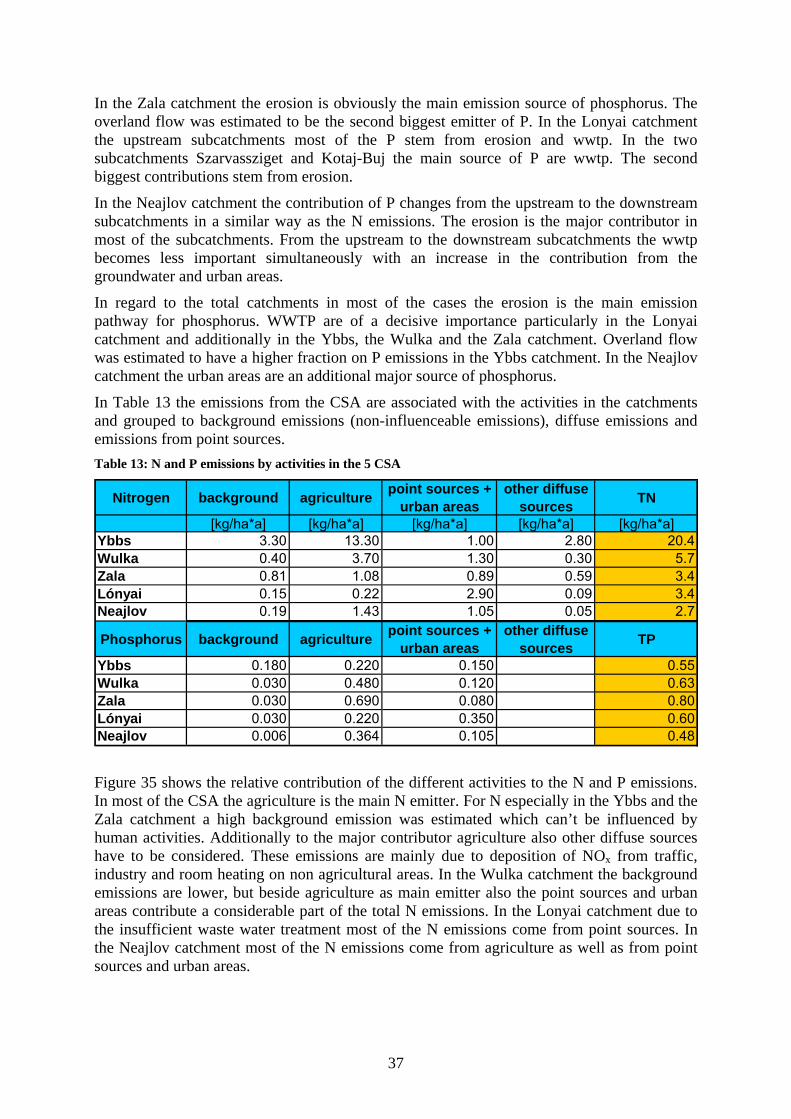
In the Zala catchment the erosion is obviously the main emission source of phosphorus. The overland flow was estimated to be the second biggest emitter of P. In the Lonyai catchment the upstream subcatchments most of the P stem from erosion and wwtp. In the two subcatchments Szarvassziget and Kotaj-Buj the main source of P are wwtp. The second biggest contributions stem from erosion.

In the Neajlov catchment the contribution of P changes from the upstream to the downstream subcatchments in a similar way as the N emissions. The erosion is the major contributor in most of the subcatchments. From the upstream to the downstream subcatchments the wwtp becomes less important simultaneously with an increase in the contribution from the groundwater and urban areas.

In regard to the total catchments in most of the cases the erosion is the main emission pathway for phosphorus. WWTP are of a decisive importance particularly in the Lonyai catchment and additionally in the Ybbs, the Wulka and the Zala catchment. Overland flow was estimated to have a higher fraction on P emissions in the Ybbs catchment. In the Neajlov catchment the urban areas are an additional major source of phosphorus.

In Table 13 the emissions from the CSA are associated with the activities in the catchments and grouped to background emissions (non-influenceable emissions), diffuse emissions and emissions from point sources. Table 13: N and P emissions by activities in the 5 CSA

Nitrogen background agriculture point sources + urban areas

other diffuse sources TN

[kg/ha*a] [kg/ha*a] [kg/ha*a] [kg/ha*a] [kg/ha*a]Ybbs 3.30 13.30 1.00 2.80 20.4Wulka 0.40 3.70 1.30 0.30 5.7Zala 0.81 1.08 0.89 0.59 3.4Lónyai 0.15 0.22 2.90 0.09 3.4Neajlov 0.19 1.43 1.05 0.05 2.7

Phosphorus background agriculture point sources + urban areas

other diffuse sources TP

Ybbs 0.180 0.220 0.150 0.55Wulka 0.030 0.480 0.120 0.63Zala 0.030 0.690 0.080 0.80Lónyai 0.030 0.220 0.350 0.60Neajlov 0.006 0.364 0.105 0.48

Figure 35 shows the relative contribution of the different activities to the N and P emissions. In most of the CSA the agriculture is the main N emitter. For N especially in the Ybbs and the Zala catchment a high background emission was estimated which can’t be influenced by human activities. Additionally to the major contributor agriculture also other diffuse sources have to be considered. These emissions are mainly due to deposition of NOx from traffic, industry and room heating on non agricultural areas. In the Wulka catchment the background emissions are lower, but beside agriculture as main emitter also the point sources and urban areas contribute a considerable part of the total N emissions. In the Lonyai catchment due to the insufficient waste water treatment most of the N emissions come from point sources. In the Neajlov catchment most of the N emissions come from agriculture as well as from point sources and urban areas.

37

0%

20%

40%

60%

80%

100%

Ybbs Wulka Zala Lónyai Neajlov

fract

ion

of T

N lo

ad [%

]

other diffusesources

pointsources /urban areas

agricluture

background

0%

20%

40%

60%

80%

100%

Ybbs Wulka Zala Lónyai Neajlov

fract

ion

on T

P lo

ad [%

]

pointsources /urban areas

agriculture

background

Figure 35: Fractions of N and P emissions by activities in the 5 case study regions

In regard to the P emissions also the agriculture is the major source for most of the case study areas. In the Ybbs catchment, there are background emissions contributing 1/3 to the total emissions. This is more than the contribution of point sources and urban areas. In the Lonyai catchment the contribution of point sources has the highest fraction on the total P emissions.

8. River loads and retention in surface waters The following chapter discusses the results from the MONERIS calculations, which were obtained in the 5 CSA in respect to the retention approaches which are included in MONERIS. In MONERIS two approaches are included to estimate the retention of nitrogen and phosphorus in the river. In both the ratio between the measured loads and the calculated emissions are used, on one approach this ratio is contrasted with the specific runoff (runoff subdivided by the area), on the other approch with the hydraulic load (runoff subdivided by the water surface area of surface waters). With the increase in specific runoff /hydraulic load the retention in the river should decrease in a certain range (see Figures: Graph / Range ± 30%).

0.00

0.25

0.50

0.75

1.00

1.25

1.50

1 10 100

specific runoff [l/(km²*s)]

TN-lo

ad/T

N-e

mis

sion

Wulka

Ybbs

ZalaLonyai DIN

Neajlov

0.00

0.25

0.50

0.75

1.00

1.25

1.50

1 10specific runoff [l/(km²*s)]

TP-lo

ad/T

P-e

mis

sion

100

Wulka

Ybbs

Zala

Lonyai

Neajlov

Figure 36: Retention of N and P in the river versus the specific runoff of the CSA

Figure 36 and Figure 37 show the relation between the retention (relation between river load and total emissions) and the specific runoff as well as the hydraulic load for N and P. Expected retention and its ranges according to the MONERIS retention approaches are compared to the retention calculated for the different subcatchments of the case study investigations. In the Ybbs and the Lonyai catchments and their subcatchments, the retention in the river is within the expected range of the MONERIS retention approach. In the Lonyai the retention is higher due to a lower specific runoff compared with the retention in the Ybbs catchment. For the Wulka, the Zala and the Neajlov catchment the retention was estimated to be out of the expected range. In all the catchments the retention in the river was calculated to be lower than according to the expectations of this retention approach. Particularly, one of the subcatchment of the Wulka catchment (Eisbach, see Table 11) and three subcatchments of the

38

Neajlov catchment (Moara din Groapa, Vadu Lat, Calugareni) have to be mentioned. In the subcatchment Eisbach, some kilometres in front of the measuring station is the location of a big point source (wwtp), what leads to a higher measured river load (consideration of in stream retention in this short section only) and is not representative for the whole river. In case of the three subcatchments of the Neajlov catchment the influence of the point sources is probably higher than it was considered in the emission calculations what leads to lower emissions as compared to the measured loads. These four catchments were not taken into account for comparison of measured and calculated loads and the related evaluation of the accuracy of the calculation, because inaccuracy for these cases can not be seen as representative for the used method.

The estimated P retention in the river for the different subcatchments does not show a good agreement with the expectations based on the retention approach with the specific runoff. Only for most of the subcatchment of the Ybbs and the Zala the retention is in a good line with the expectations. The main watershed outlet of the Ybbs catchment is out of the expected range. Emission estimates are below the measured instream loads. The reason for this is, that during the investigation period 2 major high flow events appeared, which can not be covered by the emission estimates Also the retention in the Lonyai catchment and in most of the Wulka and Neajlov catchments are not in line with the expected retention.

0.00

0.25

0.50

0.75

1.00

1.25

1.50

1 10 100 1000

hydraulic load [m/a]

TN-lo

ad/T

N-e

mis

sion

Wulka

YbbsZala

Lonyai DIN

Neajlov

0.00

0.25

0.50

0.75

1.00

1.25

1.50

1 10 100 1000

hydraulic load [m/a]

TP-lo

ad/T

P-e

mis

sion

Wulka

Ybbs

Zala

LonyaiNeajlov

Figure 37: Retention of N and P in the river versus the hydraulic load of the CSA

The N retention estimated with the approach based on the hydraulic load fits quite well with the expectations. For the Lonyai catchment the retention is higher than expected, what follows from using DIN measurements for the in stream load instead of TN, which were not available for this catchment. As mentioned before, for three subcatchments of the Neajlov point source emissions probably have been underestimated and therefore the load to emission coefficient is unrealistic high. At the Wulka in one subcatchment one point source emission only few km upstream the measuring point is influencing the load significantly. Retention figures therefore are not representative for the whole catchment. These four subcatchments have not been considered for further evaluation of data.

The retention approach based on the hydraulic load shows better accordance of the P retention with the expectations compared to the approach based on the specific runoff. Most of the subcatchments of the CSA are within the range of ± 30% of the expected retention.

For the Lonyai subcatchments no TN measurements were available. That’s why for the comparison between the calculated and measured loads the DIN (dissolved inorganic nitrogen) was used.

39

R2 = 0.9428

0

5

10

15

20

25

0 5 10 15 20 25calculatedTN-load [kg/ha.a]

TN-lo

ad [k

g/ha

.a]

WulkaYbbsLonyaiZalaNeajlov

Lonyai: DIN

R2 = 0.9778

0

5

10

15

20

25

0 5 10 15 20 25calculatedTN-load [kg/ha.a]

TN-lo

ad [k

g/ha

.a]

WulkaYbbsLonyaiZalaNeajlov

Lonyai: DIN

Figure 38: Comparison of calculated and measured nitrogen loads of different catchments with retention approach based on the specific runoff (left) and retention approach based on the hydraulic load (right)

In Figure 38 the calculated river loads using the two different retention approaches are compared to the river loads calculated from the measurements. The retention approach based on the hydraulic load fits well with the measurements and for most of the CSA the deviation is within the range of ±30%. The retention approach based on the specific runoff fits well for the Ybbs and the Lonyai catchment only. For the Wulka, the Zala and the Neajlov catchment the calculated river loads are smaller than the measured ones. Generally, the stability index is higher for the retention approach based on the hydraulic load. The trend line indicates a good estimation of the calculated loads using the retention approach based on the hydraulic load. Using the retention approach based on the specific runoff the calculated loads tend to be underestimated.

R2 = 0.5644

0.0

0.2

0.4

0.6

0.8

1.0

0 0.2 0.4 0.6 0.8 1calculatedTP-load [kg/ha.a]

TP-lo

ad [k

g/ha

.a]

WulkaYbbsLonyaiZalaNeajlov

R2 = 0.0096

0.0

0.2

0.4

0.6

0.8

1.0

0 0.2 0.4 0.6 0.8 1calculatedTP-load [kg/ha.a]

TP-lo

ad [k

g/ha

.a]

WulkaYbbsLonyaiZalaNeajlovLi (R ih 9)

Figure 39: Comparison of calculated and measured phosphorus loads of different catchments with retention approach based on the specific runoff (left) and retention approach based on the hydraulic load (right)

In regard to the phosphorus loads the retention approach based on specific runoff tends to underestimate the calculated loads (see Figure 39). Again, except the Ybbs catchment most of the catchments have a higher measured load than the calculated one. The retention approach based on the hydraulic load show a weak correlation to the phosphorus loads calculated from the measurements. For Ybbs and Lonyai the calculated river loads are below the calculated ones. For the Ybbs subcatchments this can be explained by an overrepresentation of high flow events during the investigations phase, for the Lonyai river by the high share of point source emissions, where the retention of phosphorus can be expected to be lower as from diffuse emissions. The calculated loads at the Wulka and the Zala are higher as the measured ones if the retention approach based on the hydraulic load is applied. There seems to be a tendency that the retention is overestimated. The calculated loads for the Neajlov catchment do not show a good correlation resulting in both over- and underestimations of the calculated P loads. The stability index is better for the retention approach based on the specific runoff. Generally, the retention approach based on the specific runoff tends to underestimate the calculated P load, whereas the retention approach based on the hydraulic load results a more scattered picture, where underestimation as well as overestimations appears.

40

From the results the mean deviation of the calculated loads in relation to the measured loads was calculated. All calculated mean deviations less than 30% are marked red (see Table 14). Table 14: Mean deviation of the calculated N and P loads in relation to measured loads

Ybbs [%]

Wulka [%]

Zala [%]

Lonyai [%]

Neajlov [%]

all data [%]

N-load (specific runoff) 14 60 65 31 54 47 N-load (hydraulic load) 9 22 31 13 18 16 P-load (specific runoff) 23 59 39 82 54 51 P-load (hydraulic load) 20 116 78 56 35 69

It can be seen that for all the CSA the mean deviation was calculated for the N loads using the retention approach based on the hydraulic load are within the range of 30%. That means that using this retention approach the calculated loads are well in line with the measurements. For the calculated P loads using the retention approach based on the hydraulic load for one CSA (Ybbs) the mean deviation was less than 30%.

In general, for all the data a mean deviation within the range of 30% could be obtained for the N loads using the retention approach based on the hydraulic load. For the estimation of the P loads the mean deviation for all the data was higher than 50% using both retention approaches. This result is significantly worse than the one obtained for the different subcatchments of the Basin wide MONERIS application. A reason might be that as average the subcatchments of the case study investigation are much smaller as for the Basin wide application. Due to the more dynamic behaviour of P-loads in smaller catchments the deviation between calculations and measured loads tend to increase for smaller catchments.

0

5

10

15

20

25

0 5 10 15 20 25

measured loads (kgN/(ha.a))

calc

ulat

ed E

mis

sion

s (k

g N

/(ha.

a))

Wulka basic dischargeWulka high dischargesYbbs basic dischargeYbbs high discharges1:1 Line

0,0

0,2

0,4

0,6

0,8

1,0

0,0 0,2 0,4 0,6 0,8 1,0

measured loads (kgP/(ha.a))

calc

ulat

ed E

mis

sion

s (k

gP/(h

a.a)

)

Wulka basic dischargeWulka high dischargesYbbs basic dischargeYbbs high discharges1:1 Line

Figure 40: Comparison of calculated nitrogen and phosphorus emissions and measured loads for basic discharge and high discharges in the Austrian case study regions

Above, the measured nitrogen loads of basic discharges and high discharges are plotted against calculated emissions related to basic or high discharge for different total (gross) subcatchments at the Wulka and the Ybbs. Points above the 1:1 line indicate retention during the considered conditions (emissions are higher than loads). Points below the 1:1 line indicate release of nutrients during the considered period if emission calculations and river loads are correct. For nitrogen at basic discharges retention is indicated for all subcatchments. Nitrogen emissions and river loads related to high discharges are much lower as emissions and loads related to basic discharge. For the subcatchments at the Wulka the emissions related to high discharges are almost equal to river loads related to high discharges. There is no indication for retention or release. For the subcatchments in the Ybbs loads related to high discharges are much higher than emission estimates. This would indicate release of nitrogen from the river

41

sediments under high flow conditions. Nevertheless accuracy of data is not high enough to strongly support this indication.

For phosphorus the results are quite different. Loads related to high discharges are similar to the ones related to basic discharge. For the Ybbs emission estimates for basic and high discharges are similar to the loads under the same conditions in most of the cases. This is an indication that retention is insignificant under both conditions. Only in one case there is a week indication for release of phosphorus under high flow conditions. Totally different are the results for the Wulka. The overall retention in the river system is much more important in the Wulka catchment as in the Ybbs catchment. It is evident that at high discharges emissions in the Wulka catchments are much higher than river loads. Even if a certain uncertainty for the emission estimates as well as for subdivision of river loads must be considered the indication is strong that at the Wulka emissions at high discharge conditions (mainly erosion) is retained in the river system. At basic discharges river loads are significantly higher than emissions. Emissions at basic discharges are mainly from point source. Uncertainties are comparable low for this emission pathway. Thus this indicates strongly that part of the (particulate) phosphorus emitted and retained at high discharge is released at basic discharges and increases the river loads under this conditions.

9. Evaluation of key parameters and conclusion Evaluation of key parameters and conclusions are based on the country reports on nutrient balances of case study regions (deliverable D1.3) and the comparison of results of case study investigations of different countries presented in the chapters above.

9.1. Nitrogen Groundwater is the most important pathway for nitrogen emissions into surface waters in almost all of the cases of the case study catchments and their subcatchments except in the Lonyai catchment. Point sources, urban areas and tile drainage have significant impacts (> 20 %) on the total emissions in some cases. The contribution of erosion is not very significant in all of the cases (< 20 % of total emissions) and the contribution of overland flow and direct deposition on surface water area is almost insignificant (< 5 % of total emissions) in all of the cases. In the following the key factors influencing the different pathways are discussed step by step. Finally, retention and transport of nitrogen in the river system is discussed.

Groundwater

The quantity of emissions via groundwater depends on the nitrogen surplus on agricultural soils, the surplus on non agricultural soils and the extent of retention/denitrification in soil and groundwater. The key factors influencing the nitrogen surplus in agricultural areas are mainly of anthropogenic nature: intensity of agricultural production (mainly animal density and fertilizer application) and the optimisation (time and amount) of fertiliser application and agricultural practice. The surplus on agricultural soils can be quantified based on a soil surface balance (see chapter 5.5. of deliverable D1.3; Austrian part). More advantageous for evaluation of scenarios in respect to changes of the agricultural productivity, is the “farm gate balance” (see chapter 8.2. of deliverable D1.3; Austrian part). In general, the accuracy of these calculations is appropriate. Nevertheless, it has to be stated, that the OECD method for the soil surface balance does not consider a net-mineralization. Especially in regions with a sudden drop of the production intensity net mineralization can significantly influence on the nitrogen available for leakage to groundwater on agricultural soils and can not be neglected anymore as it has been shown in the Hungarian case study investigations (see chapter 5.4. of deliverable D1.3; Hungarian part). The MONERIS approach works with long term averages

42

of the nitrogen surplus and thus, covers the effect of time delay of effects of changes in management practice on nitrogen emissions to some extent, without taking net-mineralization into account explicitly.

Key factors influencing surplus in areas not under agricultural use are anthropogenic as well: combustion processes mainly from traffic and industry as well as NH3 emissions to the air from animal husbandry which lead to nitrogen inputs by deposition.

Denitrification in groundwater highly influences nitrogen emissions to surface waters. With nitrogen surpluses on soils between 15 and 75 kgN/(ha.a) as average values for catchments, the nitrogen emissions to surface waters vary between 1 and 25 kgN/(ha.a). Denitrification in soils and groundwater of a region may amount from 5 up to more than 50 kgN/(ha.a). That means that in some regions the ratio of the surplus reaching the surface water is fewer than 5 %. The influence of denitrification in soil and groundwater on nitrogen emissions to surface waters may be higher than the anthropogenic factors leading to nitrogen surpluses in agriculture. Quantification of denitrification in groundwater therefore is the most important value in the frame of a regional nitrogen balance for surface water emissions. The natural factors influencing denitrification in soils and groundwater are hydro-geological factors as groundwater recharge rates, flow velocities and residence time in the underground, but also carbon or pyrite availability and oxygen depletion in groundwater. Denitrification by heterotrophic and autotrophic bacteria, respectively, takes place in case of degradation of organic carbon or oxidation of pyrite (FeS) under absence of dissolved oxygen. The denitrification can either be limited by the availability of organic carbon (absence or very slow hydrolyses of particulate organic matter) or pyrite or by the competition between nitrate and dissolved oxygen as electron donor for carbon degradation (diffusion limitation). Thus, it can be expected, that denitrification rates will tend to be higher if (i) the organic carbon (or pyrite) availability is high as compared to oxygen supply (oxygen and nitrate consumption), (ii) the nitrogen surplus in soils is high (high ratio nitrate to oxygen in leakage water), (iii) amount of leakage water is low (again high ratio of organic carbon or pyrite and nitrate to oxygen in leakage water) and (iv) the residence time in groundwater is high (increasing reaction time). Factor (i) depends mainly on the geological unit and the groundwater recharge rates (amount of leakage water). In factor (ii) the nitrogen surplus and in factor (iii) the groundwater recharge rates are decisive, while factor (iv) is influenced by the hydrogeological situation as well as the amount of leakage water.

The MONERIS input parameters (surplus, amount of leakage water and hydrogeological units) cover the main factors governing denitrification in underground. Results show, that on regional scale (subcatchments) the approach is able to reproduce the influence of the different hydrological and geological situations for denitrification in an appropriate way. Nevertheless, if a differentiation between different areas within a subcatchment in respect to their influence on nitrogen discharges should be calculated other approaches have to be used (see chapter 5.4. of deliverable D1.3; Austrian part). Even if the quantitative assessment has high uncertainties yet, the qualitative statement is possible, that in respect to discharges to surface waters in a catchment there are restricted areas with low flow time of groundwater to surface waters (low residence times) and which significantly contribute to nitrogen discharges to the surface waters. Other areas with long flow times of groundwater have negligible influence on river discharges of nitrogen.

Tile drainage

As for emissions via groundwater, the nitrogen surplus on soils is an important factor influencing nitrogen emissions via tile drainage. Nevertheless, the main anthropogenic factor is the amount of tile drained areas, which significantly reduce the residence time in the underground and therefore the retention/denitrification of nitrogen in the underground. A big

43

problem of quantification is that detail data on the amount of drained areas are not available in most of the regions. In the MONERIS model an approach is used to estimate amount of tile drained areas based on the soil classes. Nevertheless, even if the tiled drained area is known, the question remains, whether the tile drainage which usually was installed in the 60ies or 70ies is still working. This fact may lead to significant uncertainties of this pathway as it has been shown in the Hungarian part of deliverable D1.3 (chapter 6.2).

Point sources

The nitrogen discharges to surface waters from point sources are highly influenced by the population density and to some extent by the industrial activity in a region. These factors determine the amount of nitrogen in the waste water of a region. The head specific nitrogen emission per inhabitant is relatively constant, but may be influenced by industrial activity (see chapter 6). The share of nitrogen that is discharged to surface water via point sources depends on the waste water infrastructure of a region. Connections to sewer systems increase the share of discharges, while improvement of the treatment process from no treatment to mechanical treatment to biological treatment with carbon removal to biological treatment with nitrification and to biological treatment with nitrification/denitrification reduces the emissions.

For quantification in many cases specific data from the different points sources can be used. If this is not the case, emissions can be estimated based on information on inhabitants connected to sewer systems or population equivalents discharged to waste water, specific nitrogen emissions to waste water and typical removal rates of different treatment levels as it is presented in chapter 6. Accuracy of determination of point source emission in general is the highest as compared to other emission pathway. Estimations on specific values should be used to check existing data based on measurements. Based on this check it is possible to detect erroneous data.

Urban areas

Urban areas, as it is used as pathway in the MONERIS approach, includes three different pathways: emissions of nutrients from non sewered areas, emissions via combined sewer overflows and emissions via rain water sewers. While the emissions via rain water sewers and combined sewer overflows are usually below the calculation accuracy of total nitrogen emissions, discharges from non sewered areas may be relevant in cases, where a high portion of the population is not connected to sewer systems. Based on head specific nutrient emissions it is possible to estimate the amount of nutrients in the produced waste water relatively accurate. The problem is that usually it is not known where the waste waters from septic tanks and pits go to. Estimations based on expert knowledge have to be made. Usually most of it is leaking to the underground and groundwater and only a small part is reused in agriculture or transported to treatment plants by lorry.

The main factor controlling the emissions to the surface waters is the retention of nutrients in the leakage water in the underground and groundwater. A systematic investigation on the relation between amount of retention and the hydro-geologic situation in a region does not exist yet. Usually it is assumed, that this retention as average value is higher than 50 %. As investigation within the Hungarian case study region show this retention might be even much higher (60 – 95 % for nitrogen and > 95 % for phosphorus) in specific cases (see Deliverable D1.3, Hungarian part, chapter 5.3). This explains why on site disposal of waste water with leakage to the underground is a relatively effective “measure” in respect to nutrient discharges to surface waters. But of course it is a relevant factor for groundwater pollution (e.g. hygienic aspects).

44

Erosion

Nitrogen is transported in water mainly in soluble forms. As compared to the total emissions the content of nitrogen in relation to phosphorus is much lower. Area specific emissions are in the range of 0.1 to 0.6 kg N/(ha.a). Thus, erosion has not a significant effect in nitrogen balances and will be discussed in connection with phosphorus.

Overland flow

Overland flow (nutrient emissions via the surface runoff from non paved areas in dissolved form) is not in the focus of nitrogen balances as well. Specific emissions ranges between 0 and 0.6 kg N/(ha.a). The upper limit is found in regions with high deposition rates and a high share of surface runoff in the water balance as it can be found in the mountainous region of the Ybbs catchment.

Deposition

The pathway deposition according to the MONERIS definition is restricted to the direct deposition of nutrients on the surface waters. With emissions of 0.04 – 0.20 kg N/(ha.a) related to the total catchment area this pathway is irrelevant for nitrogen balances of land based catchments. It will become relevant only in regions with a high share of surface water area.

In contradiction to the direct deposition on the surface water area, deposition in general on agricultural and especially non agricultural areas is of significant importance as it contributes to the surplus on soils, which is basis for emissions via groundwater as it was already discussed at the emission pathway “groundwater”.

Retention and transport in surface waters

Results indicate, that the retention (difference between emissions and transported loads) in the surface waters of the case study regions lies usually between 0 and 2 kgN/(ha.a) if it is related to the total catchment area. As compared to the retention/denitrification in soil and groundwater (5 – more than 50 kg N/(ha.a)) this is relatively small. Nevertheless, retention in surface waters may influence river loads (1 – 20 kg N/(ha.a)) very significantly. In the case study areas it reduces river loads up to 75 %. Retention may be storage of nitrogen in the river corridor (wetlands, dams, floodplains) or release from the water course by denitrification. It is not possible yet to distinguish between these two forms of retention quantitatively. There is evidence that denitrification plays the major role.

In respect to denitrification from surface waters in general the same factors are decisive as for groundwater. Denitrification by heterotrophic bacteria takes place in case of degradation of organic carbon under absence of dissolved oxygen. The denitrification can either be limited by the availability of organic carbon or by the competition between nitrate and dissolved oxygen as electron donor for carbon degradation. In contradiction to the groundwater, oxygen supply in river water is much better and the reaction time is much shorter. Thus, except in cases of heavy oxygen depletion by high inputs of organic matter, denitrification in the free flowing phase of a river will by of minor importance. Denitrification will take place in side arms of wetlands, where lower residence times coincidences with high availability of carbon (algae production) and reduced supply of oxygen, and in sediments of the riverbed, as it was demonstrated in the Austrian case study areas Ybbs and Wulka (see deliverable D1.3, Austrian part, chapter 5.3). In case of exfiltration of river water through the sediments, the factors availability of carbon (sedimentation of suspended solids, e.g. algae biomass), reduced oxygen supply and increased reaction time appear and lead to significant reduction of nitrogen concentrations. The relevance for the reduction of river loads will depend on the

45

amount of water that is exchanged between surface and groundwater. The quantitative assessment of this amount was not possible within the investigations of the case studies. Qualitatively it can be stated, that in natural near river systems this exchange will be more relevant as in more canalised rivers and the relevance of this exchange will tend to increase with an increasing relation between the area surface area of the river bottom and the river discharge.

Consequently the MONERIS model uses the hydraulic load (surface water discharge of a subcatchment subdivided by surface water area) as parameter for the determination of the retention in the surface water. As it could be shown for the case study investigation on subcatchment level, based on this approach a good match between calculated river loads (emission estimations minus retention in the river) and measured river loads could be obtained. The average aberration between measured and calculated loads was 16 % for 23 subcatchments of the case study investigations. An important prerequisite for this calculation is a sound determination of the surface water area. The approach of MONERIS based on the determination of the river retention from a correlation to the areas specific runoff of a catchment needs no detailed determination surface water area, but this approach showed a much lower accordance between calculated and measured river loads. Results differ significantly from the one obtained with the “hydraulic load approach”. The average aberration between calculated and measured river loads of 23 case study subcatchments was 47 % with a clear tendency of a systematic error towards overestimation of retention and therefore lower calculated river loads as compared to measured ones.

Specific Nitrogen loads in the rivers of the case study areas vary between 1 and 20 kg N/(ha.a). Highest values are in those areas with high N-surpluses in soils and low denitrification in groundwater due to hydrogeological conditions. The measurements of nitrogen loads are not problematic, because the influence of special events on the yearly load is small. A sampling system of biweekly sampling should be appropriate for realistic results. Loads between neighbouring years can differ significantly in correlation with the different mean water discharge. In contradiction with former practice, dissolved inorganic nitrogen is not sufficient to determine total nitrogen. Organic nitrogen forms (dissolved and particulate) shall be considered. For the different case study regions organic forms of nitrogen contribute with 10 to 40 % to the total annual nitrogen loads in the rivers.

9.2. Phosphorus Erosion is the dominating pathway for phosphorus emissions into surface waters in almost all of the case study catchments and their subcatchments. Only in the Lonyai catchment the point sources are dominating. Point sources may play a remarkable role as well in other catchments. In addition, emissions via groundwater, urban areas and overland flow may reach some significance in some areas (up to 25 % contribution to total emissions). Tile drainage and deposition are of no significance in any of the subcatchments. In respect to the relevance of phosphorus for eutrophication it is important to know if phosphorus is emitted in dissolved forms or bound to particles. Erosion is clearly the pathway were particle bound phosphorus is transported. In the urban runoff both forms (dissolved and particulate) are present. From points sources mainly dissolved phosphorus is discharged. All the other pathways are dissolved forms of phosphorus only. In the following, the key factors influencing the different pathways are discussed step by step. Finally, retention and transport of nitrogen in the river system is discussed.

Erosion

The accuracy of phosphor balances of river catchments depends on the accuracy of the calculation of phosphorus inputs via soil particles by erosion. Therefore, in the daNUbs

46

project an own workpackage (wp2) is specifically dedicated to erosion estimates. For details of key factors influencing erosion see deliverable D2.2 of work package 2. From wp1 looking at P-emissions by erosion in the frame of regional nutrient balances the following conclusions can be drawn.

The surplus on agricultural soils is an important factor in respect to phosphorus emissions via erosion. This surplus is mainly determined by the amount of fertiliser applied. In contradiction to nitrogen, for phosphorus not the surplus of a year determines the potential for the emissions but the accumulation of the surplus over the years leads to increasing phosphorus content in soils. Together with the enrichment ratio of phosphorus in eroded particles (enrichment of phosphorus in small, easier erodable particles leads to higher concentrations in eroded particles than in the soil) and the amount of soil particles discharged to the river system, finally the phosphorus content in soils influences the phosphorus emissions via erosion. As it was shown for the Austrian case studies, estimations of phosphorus content in soils based on the long term phosphorus surplus in agriculture and geogenic baseline concentrations leads to quite good average soil concentrations (see chapter 5.5 of Austrian part of deliverable D1.3). The enrichment ratio for phosphorus can be determined by the relation between phosphorus content in soils and in suspended solids transported in the river system, if this data are available. Soil erosion from agricultural soils is the main emphasis of work package 2 and is not discussed here.

What should be mentioned is, that in addition to the accurate estimation of soil erosion from soils, for determination of the input into the surface water the determination of the sediment delivery ratio (ratio between eroded soil and soil particles transported into the river) is of decisive importance. Usually the sediment delivery ratio lies between 5 and 15 %. That means, only this ratio of the eroded soil reaches the surface water and that the determination of the sediment delivery ratio is more decisive for calculation of phosphorus emissions via erosion than the determination of the amount of eroded soil. A calibration of erosion estimates is only possible by a comparison of the results of erosion calculation with the transported suspended solids in the river. A problem in this respect which is not solved yet is, how to distinguish between P-retention in the catchment and retention in the river system, or expressed in a other way: which part of the sediment delivery ratio describes sedimentation before sediments reach the river system and which part describes retention after sediments have reached the river system (e.g. sedimentation in the river bed or in flooded areas). The MONERIS approach offers a practicable tool to determine the sediment delivery ratio till discharge to the river on the one hand and to estimate river retention based on an additional approach. The overall accuracy of this approach will be discussed later on (see retention and transport in the river system). Anyway, there is no way yet to check the plausibility of the differentiation between retention in the catchment and retention in the river. Further research is needed in this aspect.

Points sources and urban areas

For these two emission pathways the statements made for nitrogen are valid for phosphorus as well. Values for emissions from urban areas obtained in the case study regions vary between 0,02 – 0,09 kgP/(ha.a.) and contribute to the total emissions with less than 20 %. Even in regions with a high percentage of the population not connected to sewer systems the values are relatively low because of the high retention capacity of underground for phosphorus. P-emissions are high for points sources in those areas were a high population density coincidences with a high degree of connections to sewer systems and a low level P-removal at treatment plants.

47

Groundwater

Phosphorus emissions to surface waters via groundwater may not be neglected in all cases. In cases with a high groundwater discharge or high phosphorus concentrations in groundwater the values rise up to about 0.16 kgP/(ha.a) which may be a significant contribution to the total emissions. The MONERIS model estimates phosphorus concentrations in the groundwater based on soil types. In the Austrian case study areas in three of four cases, where the data base was appropriate for comparison, calculated phosphorus concentrations in groundwater were in line with measured groundwater concentrations (see deliverable D1.3, Austrian part, chapter 9.1). In one case phosphorus concentrations were significantly overestimated as compared to the measured values.

Overland flow

As for nitrogen, the contribution of overland flow (nutrient emissions via the surface runoff from non paved areas in dissolved form) to the total emissions for surface waters will only be of relevance (>10 %), if the water discharge via the surface is high. Area specific emission values vary between 0.003 and 0.07 kgP/(ha.a). The MONERIS model estimates the concentrations of the surface runoff based on P-saturation in soils. It was not possible in the frame of case study investigations to check an applicability of this assumption for the case study regions.

Tile drainage and deposition

Emissions via these pathways are below 0.01 kgP/(ha.a) related to the total area and are of no importance as compared to other emissions via other pathways for the subcatchments of the case study regions. Tile drainage might become important under certain conditions (high portions of tile drained areas, high P-losses from soils)

Retention and transport in surface waters

Results indicate, that the retention (difference between emissions to the river and transported loads in the river) in the surface waters of the case study regions lies between 0 and 0,7 kgP/(ha.a), if loads are related to the total catchment area. As compared to the retention in the catchment, this is relatively small. Nevertheless, retention in surface waters may influence river loads (0,2 – 1 kg P/(ha.a)) significantly. In the case study areas it reduces river loads by up to 75 %. Retention is storage of phosphorus in the river and the river corridor (wetlands, dams, floodplains). Together with emission estimates via erosion, quantification of retention in the river system is the most decisive value of a phosphorus balance for a river system.

In respect to transport of phosphorus from the catchment to the receiving Sea there is no immediate influence between phosphorus emissions via erosion and the transported loads. Retention in the river system decisively influences this transport to the Sea. Erosion events are usually in coincidence with high flow or flood events in upstream parts of a river catchment. Particle-bound phosphorus is mobilised from the catchment (erosion) and the river bottom and transported at peak discharges to downstream sections, where retention by sedimentation of particles takes place. On the one hand this retention is a transport to flooded areas. In this case it can be considered as more or less long term retention. On the other hand sedimentation takes place in the riverbed, in case the tractive effort of the river is reduced. In this second case the P-pool in the sediments of the sedimentation area will be increased. If anaerobic conditions in the sediment appear, part of the phosphorus will be transformed to soluble ortho-phosphate and will continuously contribute to the phosphorus transport to the receiving Sea. Part of the P-retained in the river sediment will be mobilised by resuspension at the next bigger high flow event. All together, these alternating processes of suspension,

48

transport, export to flooded areas or sedimentation in the river bed with partly solution and partly resuspension at the next event decreases the total phosphorus transported downstream and decreases the share of the phosphorus transport during high flow events on the total loads transported in the more downstream parts of a catchments as compared to the more upstream parts.

MONERIS model uses the hydraulic load (surface water discharge of a subcatchment subdivided by surface water area) and the areas specific runoff of a catchment as parameters for the determination of the retention in the surface water. The results of calculation of river loads differ significantly between the two approaches. For both approaches the average aberration between calculated river loads and measured ones is as average for 23 subcatchments considered in the case study investigations about 70 % (hydraulic load) and about 50 % (specific runoff) respectively. While using the retention approach with the area specific runoff this aberration clearly shows a tendency towards an underestimation of calculated loads as compared to the measured loads, the approach using the hydraulic load shows a week tendency of overestimating the calculated loads as compared to the measured loads. Definitely the relation between erosion estimates, retention in the catchment and in the river system is the main reason for the uncertainty of these calculations. In addition, the measurement of the river load is a factor of uncertainty for phosphorus. These uncertainties tend to increase with a decreasing catchment size, because the dynamic of transport processes in a river increases with decreasing catchment area. This might be an explanation why the fit between measured and calculated river loads is much better for the Basin wide application of MONERIS and the case study investigations.

It was clearly demonstrated, that high flow events significantly influence the P-load in river systems (chapter 5). Most of the P-loads are transported within few days of a year. High flood events can transport P-loads in the order of magnitude of yearly average loads. Transported loads vary a lot between different years, depending on the discharge situation of the year. Using averages over some years (e.g. 5) reduces the influence of these fluctuations. Nevertheless, it is of high importance to include high flow events into load monitoring and calculation. The influence of high flow events on the phosphorus transport decreases with increasing catchment area.

For monitoring of P-loads this means that flood events have to be specifically addressed in tributaries anyway. In a large river the importance of event oriented load monitoring depends on the time scale considered. For calculations of yearly loads monitoring at flood events is still decisive. If average loads over 5 years and more are taken into consideration, monitoring at flood events is less decisive, unless the probability of events increases significantly due to change of landuse practices in the catchment or climate change.

10. References Andreottola G., Bonomo L., Poffiali L., Zaffaroni C. (1994): A methodology for the estimation of unit nutrient and organic

loads from domestic and non-domestic sources. Europ. Wat. Pollut. Control 4 (6), pages 13-19.

Kovac A., Clement A. and Buzas K. (2004) Nutrient Balances of case study regions, Hungarian part of deliverable D1.3 of the project daNUbs, EVK1-CT-2000-00051 by the Energy, Environment and Sustainable Development (EESD) Programme of the 5th EU Framework Programme.

Lindtner, S., Nowak, O. and Kroiss, H. (2002): Benchmarking für Abwasserreinigungsanlagen. Wiener Mitteilungen, Band 176, 95-132

Lindtner S., Zessner M. (2003) Abschätzungen von Schmutzfrachten in der Abwasserentsorgung bei unvollständiger Datenlage, Wiener Mitteilungen , Band 183, Seiten 195-227, ISBN 3-85234-074-8

Nowak, O. (2000): Bilanzierung in der Abwasserreinigung, Habilitation, Technische Universität Wien.

49

Strauss, P (2004): Key factors of soil erosion, deliverable D2.2 of the project daNUbs, EVK1-CT-2000-00051 by the Energy, Environment and Sustainable Development (EESD) Programme of the 5th EU Framework Programme. Institute for Land and Water Management Research, Federal Agency for Water Management, Petzenkirchen

Zessner M. and Lindtner S. (2004) Estimations of Municipal Point Source Pollution in the Context of River Basin Management, IWA World Water Congress, 19-24 of September, Marrakech , Marokko, accepted

Zessner M., Schilling Ch., Gabriel O., Dimova G. and Lampert Ch. (2004) Nutrient Balances of case study regions, Austrian part of deliverable D1.3 of the project daNUbs, EVK1-CT-2000-00051 by the Energy, Environment and Sustainable Development (EESD) Programme of the 5th EU Framework Programme.

50