nusmv 2.2 user manualnusmv.fbk.eu/nusmv/userman/v22/nusmv.pdf · emanuele olivetti, gavin keighren,...

NuSMV 2.2 User Manual

Roberto Cavada, Alessandro Cimatti,Emanuele Olivetti, Gavin Keighren,Marco Pistore and Marco Roveri

IRST - Via Sommarive 18, 38055 Povo (Trento) – Italy

Email: [email protected]

This document is part of the distribution package of the NUSMV model checker, avail-able at http://nusmv.irst.itc.it.

Parts of this documents have been taken from “The SMV System - Draft”, by K.McMillan, available at:http://www.cs.cmu.edu/˜modelcheck/smv/smvmanual.r2.2.ps.

Copyright c�

1998-2005 by CMU and ITC-irst.

Contents

1 Introduction 4

2 Syntax 62.1 Expressions . . . . . . . . . . . . . . . . . . . . . . . . . . . . . . . 6

2.1.1 Simple Expressions . . . . . . . . . . . . . . . . . . . . . . . 62.1.2 Next Expressions . . . . . . . . . . . . . . . . . . . . . . . . 8

2.2 Definition of the FSM . . . . . . . . . . . . . . . . . . . . . . . . . . 92.2.1 State Variables . . . . . . . . . . . . . . . . . . . . . . . . . 92.2.2 Input Variables . . . . . . . . . . . . . . . . . . . . . . . . . 92.2.3 ASSIGN declarations . . . . . . . . . . . . . . . . . . . . . . 102.2.4 TRANS declarations . . . . . . . . . . . . . . . . . . . . . . 102.2.5 INIT declarations . . . . . . . . . . . . . . . . . . . . . . . 102.2.6 INVAR declarations . . . . . . . . . . . . . . . . . . . . . . 112.2.7 DEFINE declarations . . . . . . . . . . . . . . . . . . . . . . 112.2.8 ISA declarations . . . . . . . . . . . . . . . . . . . . . . . . 112.2.9 MODULE declarations . . . . . . . . . . . . . . . . . . . . . . 122.2.10 Identifiers . . . . . . . . . . . . . . . . . . . . . . . . . . . . 132.2.11 The main module . . . . . . . . . . . . . . . . . . . . . . . 142.2.12 Processes . . . . . . . . . . . . . . . . . . . . . . . . . . . . 142.2.13 FAIRNESS declarations . . . . . . . . . . . . . . . . . . . . 14

2.3 Specifications . . . . . . . . . . . . . . . . . . . . . . . . . . . . . . 152.3.1 CTL Specifications . . . . . . . . . . . . . . . . . . . . . . . 152.3.2 LTL Specifications . . . . . . . . . . . . . . . . . . . . . . . 162.3.3 Real Time CTL Specifications and Computations . . . . . . . 17

2.4 Variable Order Input . . . . . . . . . . . . . . . . . . . . . . . . . . 182.4.1 Input File Syntax . . . . . . . . . . . . . . . . . . . . . . . . 182.4.2 Scalar Variables . . . . . . . . . . . . . . . . . . . . . . . . . 192.4.3 Array Variables . . . . . . . . . . . . . . . . . . . . . . . . . 20

3 Running NuSMV interactively 213.1 Model Reading and Building . . . . . . . . . . . . . . . . . . . . . . 223.2 Commands for Checking Specifications . . . . . . . . . . . . . . . . 263.3 Commands for Bounded Model Checking . . . . . . . . . . . . . . . 313.4 Simulation Commands . . . . . . . . . . . . . . . . . . . . . . . . . 413.5 Traces . . . . . . . . . . . . . . . . . . . . . . . . . . . . . . . . . . 43

3.5.1 Inspecting Traces . . . . . . . . . . . . . . . . . . . . . . . . 443.5.2 Displaying Traces . . . . . . . . . . . . . . . . . . . . . . . 443.5.3 Trace Plugin Commands . . . . . . . . . . . . . . . . . . . . 44

2

3.6 Trace Plugins . . . . . . . . . . . . . . . . . . . . . . . . . . . . . . 463.6.1 Basic Trace Explainer . . . . . . . . . . . . . . . . . . . . . 463.6.2 States/Variables Table . . . . . . . . . . . . . . . . . . . . . 473.6.3 XML Format Printer . . . . . . . . . . . . . . . . . . . . . . 473.6.4 XML Format Reader . . . . . . . . . . . . . . . . . . . . . . 48

3.7 Interface to the DD Package . . . . . . . . . . . . . . . . . . . . . . 483.8 Administration Commands . . . . . . . . . . . . . . . . . . . . . . . 523.9 Other Environment Variables . . . . . . . . . . . . . . . . . . . . . . 60

4 Running NuSMV batch 63

A Compatibility with CMU SMV 68

3

Chapter 1

Introduction

NUSMV is a symbolic model checker originated from the reengineering, reimplemen-tation and extension of CMU SMV, the original BDD-based model checker developedat CMU [McM93]. The NUSMV project aims at the development of a state-of-the-artsymbolic model checker, designed to be applicable in technology transfer projects: itis a well structured, open, flexible and documented platform for model checking, andis robust and close to industrial systems standards [CCGR00].

Version 1 of NUSMV basically implements BDD-based symbolic model check-ing. Version 2 of NUSMV (NUSMV2 in the following) inherits all the functionalitiesof the previous version, and extend them in several directions [CCG � 02]. The mainnovelty in NUSMV2 is the integration of model checking techniques based on proposi-tional satisfiability (SAT) [BCCZ99]. SAT-based model checking is currently enjoyinga substantial success in several industrial fields, and opens up new research directions.BDD-based and SAT-based model checking are often able to solve different classes ofproblems, and can therefore be seen as complementary techniques.

Starting from NUSMV2, we are also adopting a new development and licensemodel. NUSMV2 is distributed with an OpenSource license1, that allows anyoneinterested to freely use the tool and to participate in its development. The aim ofthe NUSMV OpenSource project is to provide to the model checking community acommon platform for the research, the implementation, and the comparison of newsymbolic model checking techniques. Since the release of NUSMV2, the NUSMVteam has received code contributions for different parts of the system. Several researchinstitutes and commercial companies have express interest in collaborating to the de-velopment of NUSMV. The main features of NUSMV are the following:

� Functionalities. NUSMV allows for the representation of synchronous andasynchronous finite state systems, and for the analysis of specifications expressedin Computation Tree Logic (CTL) and Linear Temporal Logic (LTL), usingBDD-based and SAT-based model checking techniques. Heuristics are avail-able for achieving efficiency and partially controlling the state explosion. Theinteraction with the user can be carried on with a textual interface, as well as inbatch mode.

� Architecture. A software architecture has been defined. The different compo-nents and functionalities of NUSMV have been isolated and separated in mod-

1(see http://www.opensource.org)

4

ules. Interfaces between modules have been provided. This reduces the effortneeded to modify and extend NUSMV.

� Quality of the implementation. NUSMV is written in ANSI C, is POSIX com-pliant, and has been debugged with Purify in order to detect memory leaks. Fur-thermore, the system code is thoroughly commented. NUSMV uses the stateof the art BDD package developed at Colorado University, and provides a gen-eral interface for linking with state-of the-art SAT solvers. This makes NUSMVvery robust, portable, efficient, and easy to understand by other people than thedevelopers.

This document is structured as follows.

� In Chapter 2 [Syntax], page 6 we define the syntax of the input language ofNUSMV.

� In Chapter 3 [Running NuSMV interactively], page 21 the commands of theinteraction shell are described.

� In Chapter 4 [Running NuSMV batch], page 63 we define the batch mode ofNUSMV.

NUSMV is available at http://nusmv.irst.itc.it.

5

Chapter 2

Syntax

We present now the complete syntax of the input language of NUSMV. In the follow-ing, an atom may be any sequence of characters starting with a character in the set�A-Za-z � and followed by a possibly empty sequence of characters belonging to the

set�A-Za-z0-9 $#- �� . A number is any sequence of digits. A digit belongs to the

set�0-9 � .

All characters and case in a name are significant. Whitespace characters are space(<SPACE>), tab (<TAB>) and newline (<RET>). Any string starting with two dashes(‘--’) and ending with a newline is a comment. Any other tokens recognized by theparser are enclosed in quotes in the syntax expressions below. Grammar productionsenclosed in square brackets (‘[]’) are optional.

2.1 Expressions

Expressions are constructed from variables, constants, and a collection of operators,including boolean connectives, integer arithmetic operators, case expressions and setexpressions.

2.1.1 Simple Expressions

Simple expressions are expressions built only from current state variables. Simpleexpressions can be used to specify sets of states, e.g. the initial set of states. Thesyntax of simple expressions is as follows:

simple_expr ::atom ;; a symbolic constant

| number ;; a numeric constant| "TRUE" ;; The boolean constant 1| "FALSE" ;; The boolean constant 0| var_id ;; a variable identifier| "(" simple_expr ")"| "!" simple_expr ;; logical not| simple_expr "&" simple_expr ;; logical and| simple_expr "|" simple_expr ;; logical or| simple_expr "xor" simple_expr ;; logical exclusive or| simple_expr "->" simple_expr ;; logical implication| simple_expr "<->" simple_expr ;; logical equivalence

6

| simple_expr "=" simple_expr ;; equality| simple_expr "!=" simple_expr ;; inequality| simple_expr "<" simple_expr ;; less than| simple_expr ">" simple_expr ;; greater than| simple_expr "<=" simple_expr ;; less than or equal| simple_expr ">=" simple_expr ;; greater than or equal| simple_expr "+" simple_expr ;; integer addition| simple_expr "-" simple_expr ;; integer subtraction| simple_expr "*" simple_expr ;; integer multiplication| simple_expr "/" simple_expr ;; integer division| simple_expr "mod" simple_expr ;; integer remainder| set_simple_expr ;; a set simple_expression| case_simple_expr ;; a case expression

A var id, (see Section 2.2.10 [Identifiers], page 13) or identifier, is a symbol or expres-sion which identifies an object, such as a variable or a defined symbol. Since a var idcan be an atom, there is a possible ambiguity if a variable or defined symbol has thesame name as a symbolic constant. Such an ambiguity is flagged by the interpreter asan error.

The order of parsing precedence for operators from high to low is:

*,/+,-mod=,!=,<,>,<=,>=|,xor<->->

Operators of equal precedence associate to the left, except -> that associates to theright. Parentheses may be used to group expressions.

Case Expressions

A case expression has the following syntax:

case_simple_expr ::"case"

simple_expr ":" simple_expr ";"simple_expr ":" simple_expr ";"...simple_expr ":" simple_expr ";"

"esac"

A case simple expr returns the value of the first expression on the right handside of ‘:’, such that the corresponding condition on the left hand side evaluates to 1.Thus, if simple expr on the left side is true, then the result is the correspondingsimple expr on the right side. If none of the expressions on the left hand sideevaluates to 1, the result of the case expression is the numeric value 1. It isan error for any expression on the left hand side to return a value other than the truthvalues 0 or 1.

Set Expressions

A set expression has the following syntax:

7

set_expr ::" � " set_elem "," ... "," set_elem " � " ;; set definition

| simple_expr "in " simple_expr ;; set inclusion test| simple_expr "union " simple_expr ;; set union

set_elem :: simple_expr

A set can be defined by enumerating its elements inside curly braces ‘�. . . � ’. The

inclusion operator ‘in’ tests a value for membership in a set. The union operator‘union’ takes the union of two sets. If either argument is a number or a symbolicvalue instead of a set, it is coerced to a singleton set.

2.1.2 Next Expressions

While simple expressions can represent sets of states, next expressions relate currentand next state variables to express transitions in the FSM. The structure of next ex-pressions is similar to the structure of simple expressions (See Section 2.1.1 [simpleexpressions], page 6). The difference is that next expression allow to refer to next statevariables. The grammar is depicted below.

next_expr ::atom ;; a symbolic constant

| number ;; a numeric constant| "TRUE" ;; The boolean constant 1| "FALSE" ;; The boolean constant 0| var_id ;; a variable identifier| "(" next_expr ")"| "next" "(" simple_expr ")" ;; next value of an "expression"| "!" next_expr ;; logical not| next_expr "&" next_expr ;; logical and| next_expr "|" next_expr ;; logical or| next_expr "xor" next_expr ;; logical exclusive or| next_expr "->" next_expr ;; logical implication| next_expr "<->" next_expr ;; logical equivalence| next_expr "=" next_expr ;; equality| next_expr "!=" next_expr ;; inequality| next_expr "<" next_expr ;; less than| next_expr ">" next_expr ;; greater than| next_expr "<=" next_expr ;; less than or equal| next_expr ">=" next_expr ;; greater than or equal| next_expr "+" next_expr ;; integer addition| next_expr "-" next_expr ;; integer subtraction| next_expr "*" next_expr ;; integer multiplication| next_expr "/" next_expr ;; integer division| next_expr "mod" next_expr ;; integer remainder| set_next_expr ;; a set next_expression| case_next_expr ;; a case expression

set next expr and case next expr are the same as set simple expr (seeSection 2.1.1 [set expressions], page 7) and case simple expr (see Section 2.1.1[case expressions], page 7) respectively, with the replacement of ”simple ” with”next ”. The only additional production is "next" "(" simple expr ")",which allows to “shift” all the variables in simple expr to the next state. The nextoperator distributes on every operator. For instance, the formula next((A & B) |

8

C) is a shorthand for the formula (next(A) & next(B)) | next(C). It is anerror if in the scope of the next operator occurs another next operator.

2.2 Definition of the FSM

2.2.1 State Variables

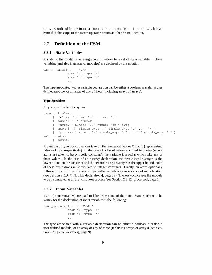
A state of the model is an assignment of values to a set of state variables. Thesevariables (and also instances of modules) are declared by the notation:

var_declaration :: "VAR "atom ":" type ";"atom ":" type ";"...

The type associated with a variable declaration can be either a boolean, a scalar, a userdefined module, or an array of any of these (including arrays of arrays).

Type Specifiers

A type specifier has the syntax:

type :: boolean| " � " val "," val "," ... val " � "| number ".." number| "array " number ".." number "of " type| atom [ "(" simple_expr "," simple_expr "," ... ")" ]| "process " atom [ "(" simple_expr "," ... "," simple_expr ")" ]

val :: atom| number

A variable of type boolean can take on the numerical values 0 and 1 (representingfalse and true, respectively). In the case of a list of values enclosed in quotes (whereatoms are taken to be symbolic constants), the variable is a scalar which take any ofthese values. In the case of an array declaration, the first simple expr is thelower bound on the subscript and the second simple expr is the upper bound. Bothof these expressions must evaluate to integer constants. Finally, an atom optionallyfollowed by a list of expressions in parentheses indicates an instance of module atom(see Section 2.2.9 [MODULE declarations], page 12). The keyword causes the moduleto be instantiated as an asynchronous process (see Section 2.2.12 [processes], page 14).

2.2.2 Input Variables

IVAR (input variables) are used to label transitions of the Finite State Machine. Thesyntax for the declaration of input variables is the following:

ivar_declaration :: "IVAR "atom ":" type ";"atom ":" type ";"...

The type associated with a variable declaration can be either a boolean, a scalar, auser defined module, or an array of any of these (including arrays of arrays) (see Sec-tion 2.2.1 [state variables], page 9).

9

2.2.3 ASSIGN declarations

An assignment has the form:

assign_declaration :: "ASSIGN "assign_body ";"assign_body ";"...

assign_body ::atom ":=" simple_expr ;; normal assignment

| "init" "(" atom ")" ":=" simple_expr ;; init assignment| "next" "(" atom ")" ":=" next_expr ;; next assignment

On the left hand side of the assignment, atom denotes the current value of a variable,‘init(atom)’ denotes its initial value, and ‘next(atom)’ denotes its value in the next state.If the expression on the right hand side evaluates to an integer or symbolic constant,the assignment simply means that the left hand side is equal to the right hand side. Onthe other hand, if the expression evaluates to a set, then the assignment means that theleft hand side is contained in that set. It is an error if the value of the expression is notcontained in the range of the variable on the left hand side.

In order for a program to be implementable, there must be some order in whichthe assignments can be executed such that no variable is assigned after its value isreferenced. This is not the case if there is a circular dependency among the assignmentsin any given process. Hence, such a condition is an error. It is also an error for a variableto be assigned more than once at any given time. More precisely, it is an error if any ofthe following occur:

� the next or current value of a variable is assigned more than once in a givenprocess

� the initial value of a variable is assigned more than once in the program

� the current value and the initial value of a variable are both assigned in the pro-gram

� the current value and the next value of a variable are both assigned in the program

2.2.4 TRANS declarations

The transition relation � of the model is a set of current state/next state pairs. Whetheror not a given pair is in this set is determined by a boolean valued expression � , intro-duced by the ‘TRANS’ keyword. The syntax of a TRANS declaration is:

trans_declaration :: "TRANS " trans_expr [";"]trans_expr :: next_expr

It is an error for the expression to yield any value other than 0 or 1. If there is morethan one TRANS declaration, the transition relation is the conjunction of all of TRANSdeclarations.

2.2.5 INIT declarations

The set of initial states of the model is determined by a boolean expression under the‘INIT’ keyword. The syntax of a INIT declaration is:

10

init_declaration :: "INIT " init_expr [";"]init_expr :: simple_expr

It is an error for the expression to contain the next() operator, or to yield any valueother than 0 or 1. If there is more than one INIT declaration, the initial set is theconjunction of all of the INIT declarations.

2.2.6 INVAR declarations

The set of invariant states (i.e. the analogous of normal assignments, as describedin Section 2.2.3 [ASSIGN declarations], page 10) can be specified using a booleanexpression under the ‘INVAR’ keyword. The syntax of a INVAR declaration is:

invar_declaration :: "INVAR " invar_expr [";"]invar_expr :: simple_expr

It is an error for the expression to contain the next() operator, or to yield any valueother than 0 or 1. If there is more than one INVAR declaration, the invariant set is theconjunction of all of the INVAR declarations.

2.2.7 DEFINE declarations

In order to make descriptions more concise, a symbol can be associated with a com-monly expression. The syntax for this kind of declaration is:

define_declaration :: "DEFINE "atom ":=" simple_expr ";"atom ":=" simple_expr ";"...atom ":=" simple_expr ";"

Whenever an identifier referring to the symbol on the left hand side of the ‘:=’ ina DEFINE occurs in an expression, it is replaced by the expression on the right handside. The expression on the right hand side is always evaluated in its context (see Sec-tion 2.2.9 [MODULE declarations], page 12 for an explanation of contexts). Forwardreferences to defined symbols are allowed, but circular definitions are not allowed, andresult in an error.

It is not possible to assign values to defined symbols non-deterministically. Anotherdifference between defined symbols and variables is that while variables are staticallytyped, definitions are not.

2.2.8 ISA declarations

There are cases in which some parts of a module could be shared among differentmodules, or could be used as a module themselves. In NUSMV it is possible to declarethe common parts as separate modules, and then use the ISA declaration to import thecommon parts inside a module declaration. The syntax of an ISA declaration is asfollows:

isa_declaration :: "ISA " atom

where atom must be the name of a declared module. The ISA declaration can bethought as a simple macro expansion command, because the body of the module refer-enced by an ISA command is replaced to the ISA declaration.

11

2.2.9 MODULE declarations

A module is an encapsulated collection of declarations. Once defined, a module canbe reused as many times as necessary. Modules can also be so that each instance ofa module can refer to different data values. A module can contain instances of othermodules, allowing a structural hierarchy to be built. The syntax of a module declarationis as follows.

module :: "MODULE " atom [ "(" atom "," atom "," ... atom ")" ][ var_declaration ][ ivar_declaration ][ assign_declaration ][ trans_declaration ][ init_declaration ][ invar_declaration ][ spec_declaration ][ checkinvar_declaration ][ ltlspec_declaration ][ compute_declaration ][ fairness_declaration ][ define_declaration ][ isa_declaration ]

The atom immediately following the keyword ”MODULE ” is the name associated withthe module. Module names are drawn from a separate name space from other names inthe program, and hence may clash with names of variables and definitions. The optionallist of atoms in parentheses are the formal parameters of the module. Whenever theseparameters occur in expressions within the module, they are replaced by the actualparameters which are supplied when the module is instantiated (see below).

An instance of a module is created using the VAR declaration (see Section 2.2.1[state variables], page 9). This declaration supplies a name for the instance, and alsoa list of actual parameters, which are assigned to the formal parameters in the moduledefinition. An actual parameter can be any legal expression. It is an error if the numberof actual parameters is different from the number of formal parameters. The semanticof module instantiation is similar to call-by-reference. For example, in the followingprogram fragment:

MODULE main...VARa : boolean;b : foo(a);

...MODULE foo(x)ASSIGN

x := 1;

the variable a is assigned the value 1. This distinguishes the call-by-reference mecha-nism from a call-by-value scheme.Now consider the following program:

MODULE main...DEFINE

12

a := 0;VAR

b : bar(a);...MODULE bar(x)DEFINE

a := 1;y := x;

In this program, the value of y is 0. On the other hand, using a call-by-name mech-anism, the value of y would be 1, since a would be substituted as an expression forx.Forward references to module names are allowed, but circular references are not, andresult in an error.

2.2.10 Identifiers

An id, or identifier, is an expression which references an object. Objects are instancesof modules, variables, and defined symbols. The syntax of an identifier is as follows.

id :: atom| "self"| id "." atom| id "[" simple_expr "]"

An atom identifies the object of that name as defined in a VAR or DEFINE declaration.If a identifies an instance of a module, then the expression ‘a.b’ identifies the com-ponent object named ‘b’ of instance ‘a’. This is precisely analogous to accessing acomponent of a structured data type. Note that an actual parameter of module ‘a’ canidentify another module instance ‘b’, allowing ‘a’ to access components of ‘b’, as inthe following example:

MODULE main... VAR

a : foo(b);b : bar(a);

...MODULE foo(x)DEFINE

c := x.p | x.q;MODULE bar(x)VAR

p : boolean;q : boolean;

Here, the value of ‘c’ is the logical or of ‘p’ and ‘q’.If ‘a’ identifies an array, the expression ‘a[b]’ identifies element ‘b’ of array ‘a’. Itis an error for the expression ‘b’ to evaluate to a number outside the subscript boundsof array ‘a’, or to a symbolic value.

It is possible to refer the name the current module has been instantiated to by usingthe self builtin identifier.

MODULE element(above, below, token)VAR

13

Token : boolean;ASSIGN

init(Token) := token;next(Token) := token-in;

DEFINEabove.token-in := Token;grant-out := below.grant-out;

MODULE cellVAR

e2 : element(self, e1, 0);e1 : element(e1 , self, 1);

DEFINEe2.token-in := token-in;grant-out := grant-in & !e1.grant-out;

MODULE mainVAR c1 : cell;

In this example the name the cell module has been instantiated to is passed to thesubmodule element. In the main module, declaring c1 to be an instance of mod-ule cell and defining above.token-in in module e2, really amounts to defin-ing the symbol c1.token-in. When you, in the cell module, declare e1 to bean instance of module element, and you define grant-out in module e1 to bebelow.grant-out, you are really defining it to be the symbol c1.grant-out.

2.2.11 The main module

The syntax of a NUSMV program is:

program ::module_1module_2...module_n

There must be one module with the name main and no formal parameters. The modulemain is the one evaluated by the interpreter.

2.2.12 Processes

Processes are used to model interleaving concurrency. A process is a module which isinstantiated using the keyword ‘process’ (see Section 2.2.1 [state variables], page 9).The program executes a step by non-deterministically choosing a process, then execut-ing all of the assignment statements in that process in parallel. It is implicit that if agiven variable is not assigned by the process, then its value remains unchanged. Eachinstance of a process has a special boolean variable associated with it called running.The value of this variable is 1 if and only if the process instance is currently selectedfor execution. A process may run only when its parent is running. In addition no twoprocesses with the same parents may be running at the same time.

2.2.13 FAIRNESS declarations

A fairness constraint restricts the attention only to fair execution paths. When evalu-ating specifications, the model checker considers path quantifiers to apply only to fairpaths.

14

NUSMV supports two types of fairness constraints, namely justice constraints andcompassion constraints. A justice constraint consists of a formula f which is assumedto be true infinitely often in all the fair paths. In NUSMV justice constraints are iden-tified by keywords JUSTICE and, for backward compatibility, FAIRNESS. A com-passion constraint consists of a pair of formulas (p,q); if property p is true infinitelyoften in a fair path, then also formula q has to be true infinitely often in the fair path. InNUSMV compassion constraints are identified by keyword COMPASSION.1 If com-passion constraints are used then the model must not contain any input variables. Cur-rently, NUSMV does not enforce this so it is the responsibility of the user to make surethat this is the case.

Fairness constraints are declared using the following syntax:

fairness_declaration ::"FAIRNESS " simple_expr [";"]

| "JUSTICE " simple_expr [";"]| "COMPASSION " "(" simple_expr "," simple_expr ")" [";"]

A path is considered fair if and only if it satisfies all the constraints declared in thismanner.

2.3 Specifications

The specifications to be checked on the FSM can be expressed in two different tem-poral logics: the Computation Tree Logic CTL, and the Linear Temporal Logic LTLextended with Past Operators. It is also possible to analyze quantitative characteristicsof the FSM by specifying real-time CTL specifications. Specifications can be posi-tioned within modules, in which case they are preprocessed to rename the variablesaccording to the containing context.

CTL and LTL specifications are evaluated by NUSMV in order to determine theirtruth or falsity in the FSM. When a specification is discovered to be false, NUSMVconstructs and prints a counterexample, i.e. a trace of the FSM that falsifies the prop-erty.

2.3.1 CTL Specifications

A CTL specification is given as a formula in the temporal logic CTL, introduced by thekeyword ‘SPEC’. The syntax of this declaration is:

spec_declaration :: "SPEC " spec_expr [";"]spec_expr :: ctl_expr

The syntax of CTL formulas recognized by the NUSMV parser is as follows:

ctl_expr ::simple_expr ;; a simple boolean expression| "(" ctl_expr ")"| "!" ctl_expr ;; logical not| ctl_expr "&" ctl_expr ;; logical and| ctl_expr "|" ctl_expr ;; logical or

1In the current version of NUSMV, compassion constraints are supported only for BDD-based LTLmodel checking. We plan to add support for compassion constraints also for CTL specifications and inBounded Model Checking in the next releases of NUSMV.

15

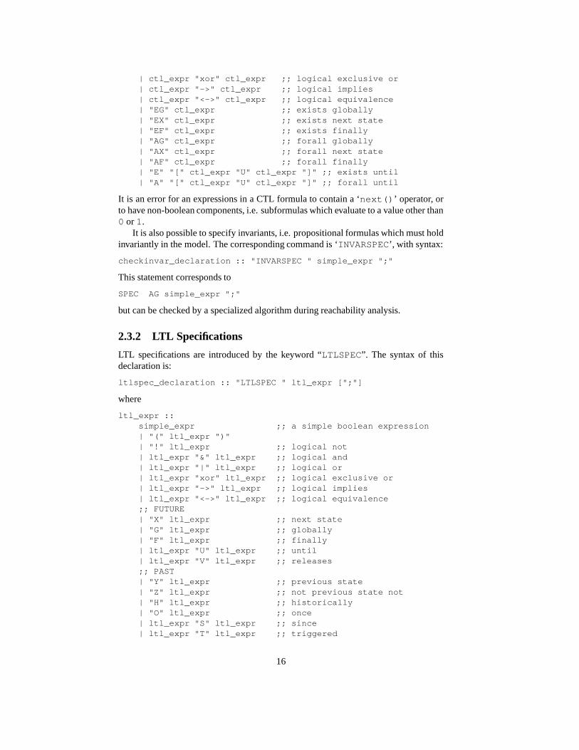
| ctl_expr "xor" ctl_expr ;; logical exclusive or| ctl_expr "->" ctl_expr ;; logical implies| ctl_expr "<->" ctl_expr ;; logical equivalence| "EG" ctl_expr ;; exists globally| "EX" ctl_expr ;; exists next state| "EF" ctl_expr ;; exists finally| "AG" ctl_expr ;; forall globally| "AX" ctl_expr ;; forall next state| "AF" ctl_expr ;; forall finally| "E" "[" ctl_expr "U" ctl_expr "]" ;; exists until| "A" "[" ctl_expr "U" ctl_expr "]" ;; forall until

It is an error for an expressions in a CTL formula to contain a ‘next()’ operator, orto have non-boolean components, i.e. subformulas which evaluate to a value other than0 or 1.

It is also possible to specify invariants, i.e. propositional formulas which must holdinvariantly in the model. The corresponding command is ‘INVARSPEC’, with syntax:

checkinvar_declaration :: "INVARSPEC " simple_expr ";"

This statement corresponds to

SPEC AG simple_expr ";"

but can be checked by a specialized algorithm during reachability analysis.

2.3.2 LTL Specifications

LTL specifications are introduced by the keyword “LTLSPEC”. The syntax of thisdeclaration is:

ltlspec_declaration :: "LTLSPEC " ltl_expr [";"]

where

ltl_expr ::simple_expr ;; a simple boolean expression| "(" ltl_expr ")"| "!" ltl_expr ;; logical not| ltl_expr "&" ltl_expr ;; logical and| ltl_expr "|" ltl_expr ;; logical or| ltl_expr "xor" ltl_expr ;; logical exclusive or| ltl_expr "->" ltl_expr ;; logical implies| ltl_expr "<->" ltl_expr ;; logical equivalence;; FUTURE| "X" ltl_expr ;; next state| "G" ltl_expr ;; globally| "F" ltl_expr ;; finally| ltl_expr "U" ltl_expr ;; until| ltl_expr "V" ltl_expr ;; releases;; PAST| "Y" ltl_expr ;; previous state| "Z" ltl_expr ;; not previous state not| "H" ltl_expr ;; historically| "O" ltl_expr ;; once| ltl_expr "S" ltl_expr ;; since| ltl_expr "T" ltl_expr ;; triggered

16

In NUSMV, LTL specifications can be analyzed both by means of BDD-based reason-ing, or by means of SAT-based bounded model checking. In the first case, NUSMVproceeds along the lines described in [CGH97]. For each LTL specification, a tableauable to recognize the behaviors falsifying the property is constructed, and then syn-chronously composed with the model. With respect to [CGH97], the approach is fullyintegrated within NUSMV, and allows for full treatment of past temporal operators.In the case of BDD-based reasoning, the counterexample generated to show the fal-sity of a LTL specification may contain state variables which have been introduced bythe tableau construction procedure. In the second case, a similar tableau constructionis carried out to encode the existence of a path of limited length violating the prop-erty. NUSMV generates a propositional satisfiability problem, that is then tackled bymeans of an efficient SAT solver [BCCZ99]. In both cases, the tableau constructionsare completely transparent to the user.

2.3.3 Real Time CTL Specifications and Computations

NUSMV allows for Real Time CTL specifications [EMSS91]. NUSMV assumes thateach transition takes unit time for execution. RTCTL extends the syntax of CTL pathexpressions with the following bounded modalities:

rtctl_expr ::ctl_expr

| "EBF" range rtctl_expr| "ABF" range rtctl_expr| "EBG" range rtctl_expr| "ABG" range rtctl_expr| "A" "[" rtctl_expr "BU" range rtctl_expr "]"| "E" "[" rtctl_expr "BU" range rtctl_expr "]"

range :: number ".." number"

Intuitively, the semantics of the RTCTL operators is as follows:

� EBF m..n p requires that there exists a path starting from a state, such thatproperty p holds in a future time instant i, with �

��

� ABF m..n p requires that for all paths starting from a state, property p holdsin a future time instant i, with �

��

� EBG m..n p requires that there exists a path starting from a state, such thatproperty p holds in all future time instants i, with �

��

� ABG m..n p requires that for all paths starting from a state, property p holdsin all future time instants i, with �

��

� E [ p BU m..n q ] requires that there exists a path starting from a state,such that property q holds in a future time instant i, with �

��, and

property p holds in all future time instants j, with ��

� A [ p BU m..n q ], requires that for all paths starting from a state, prop-erty q holds in a future time instant i, with �

��, and property p holds in

all future time instants j, with ��

Real time CTL specifications can be defined with the following syntax, which extendsthe syntax for CTL specifications.

17

spec_declaration :: "SPEC " rtctl_expr [";"]

With the ‘COMPUTE’ statement, it is also possible to compute quantitative informa-tion on the FSM. In particular, it is possible to compute the exact bound on the delaybetween two specified events, expressed as CTL formulas. The syntax is the following:

compute_declaration :: "COMPUTE " compute_expr [";"]

where

compute_expr :: "MIN" "[" rtctl_expr "," rtctl_expr "]"| "MAX" "[" rtctl_expr "," rtctl_expr "]"

MIN [start , final] computes the set of states reachable from start. If at anypoint, we encounter a state satisfying final, we return the number of steps taken to reachthe state. If a fixed point is reached and no states intersect final then infinity is returned.MAX [start , final] returns the length of the longest path from a state in startto a state in final. If there exists an infinite path beginning in a state in start that neverreaches a state in final, then infinity is returned.

2.4 Variable Order Input

It is possible to specify the order in which variables should appear in the BDD’s gen-erated by NUSMV. The file which gives the desired order can be read in using the -ioption in batch mode or by setting the input order file environment variable ininteractive mode.

2.4.1 Input File Syntax

The syntax for input files describing the desired variable ordering is as follows, wherethe file can be considered as a list of variable names, each of which must be on aseparate line:

vars_list :: EMPTY| var_list_item vars_list

var_list_item :: var_main_id| var_main_id.NUMBER

var_main_id :: ATOM| var_main_id[NUMBER]| var_main_id.var_id

var_id :: ATOM| var_id[NUMBER]| var_id.var_id

That is, a list of variable names of the following forms:

Complete_Var_Name - to specify an ordinary variableComplete_Var_Name[index] - to specify an array variable elementComplete_Var_Name.NUMBER - to specify a specific bit of an encoded

scalar variable

18

where Complete Var Name is just the name of the variable if it appears in the mod-ule MAIN, otherwise it has the module name(s) prepended to the start, for example:

mod1.mod2...modN.varname

where varname is a variable in modN, and modN.varname is a variable in modN-1,and so on. Note that the module name main is implicitely prepended to every variablename and therefore must not be included in their declarations.Any variable which appears in the model file, but not the ordering file is placed afterall the others in the ordering. Variables which appear in the ordering file but not themodel file are ignored. In both cases NUSMV displays a warning message statingthese actions.

Comments can be included by using the same syntax as regular NUSMV files. Thatis, by starting the line with --.

2.4.2 Scalar Variables

A variable which has a finite range of values that it can take is encoded as a set ofboolean variables. These boolean variables represent the binary equivalents of all thepossible values for the scalar variable. Thus, a scalar variable that can take values from0 to 7 would require three boolean variables to represent it.

It is possible to not only declare the position of a scalar variable in the ordering file,but each of the boolean variables which represent it.If only the scalar variable itself is named then all the boolean variables which are actu-ally used to encode it are grouped together in the BDD.Variables which are grouped together will always remain next to each other in the BDDand in the same order. When dynamic variable re-ordering is carried out, the group ofvariables are treated as one entity and moved as such.If a scalar variable is omitted from the ordering file then it will be added at the endof the variable order and the specific-bit variables that represent it will be groupedtogether. However, if any specific-bit variables have been declared in the ordering file(see below) then these will not be grouped with the remaining ones.It is also possible to specify that specific-bit variables are placed elsewhere in the order-ing. This is achieved by first specifying the scalar variable name in the desired location,then simply specifying Complete Var Name.i at the position where you want thatbit variable to appear:

...Complete Var Name...Complete Var Name.i...

The result of doing this is that the variable representing the��

bit is located in adifferent position to the remainder of the variables representing the rest of the bits.The specific-bit variables varname.0, ..., varname.i-1, varname.i+1, ..., varname.N aregrouped together as before.

If any one bit occurs before the variable it belongs to, the remaining specific-bitvariables are not grouped together:

...

19

Complete Var Name.i...Complete Var Name...

The variable representing the� ��

bit is located at the position given in the variableordering and the remainder are located where the scalar variable name is declared. Inthis case, the remaining bit variables will not be grouped together.This is just a short-hand way of writing each individual specific-bit variable in theordering file. The following are equivalent:

... ...Complete Var Name.0 Complete Var Name.0Complete Var Name.1 Complete Var Name: ...Complete Var Name.N-1...

where the scalar variable Complete Var Name requires N boolean variables to en-code all the possible values that it may take.

It is still possible to then specify other specific-bit variables at later points in the or-dering file as before.

2.4.3 Array Variables

When declaring array variables in the ordering file, each individual element must bespecified separately. It is not permitted to specify just the name of the array.

The reason for this is that the actual definition of an array in the model file is essentiallya shorthand method of defining a list of variables that all have the same type. Nothingis gained by declaring it as an array over declaring each of the elements individually,and there is no difference in terms of the internal representation of the variables.

20

Chapter 3

Running NuSMV interactively

The main interaction mode of NUSMV is through an interactive shell. In this modeNUSMV enters a read-eval-print loop. The user can activate the various NUSMV com-putation steps as system commands with different options. These steps can thereforebe invoked separately, possibly undone or repeated under different modalities. Thesesteps include the construction of the model under different partitioning techniques,model checking of specifications, and the configuration of the BDD package. The in-teractive shell of NUSMV is activated from the system prompt as follows (’NuSMV>’is the default NUSMV shell prompt):

system prompt> NuSMV -int <RET>NuSMV>

A NUSMV command is a sequence of words. The first word specifies the com-mand to be executed. The remaining words are arguments to the invoked command.Commands separated by a ‘;’ are executed sequentially; the NUSMV shell waits foreach command to terminate in turn. The behavior of commands can depend on envi-ronment variables, similar to “csh” environment variables.

In the following we present the possible commands followed by the related envi-ronment variables, classified in different categories. Every command answers to theoption -h by printing out the command usage. When output is paged for some com-mands (option -m), it is piped through the program specified by the UNIX PAGER shellvariable, if defined, or through the UNIX command “more”. Environment variables canbe assigned a value with the “set” command. Command sequences to NUSMV mustobey the (partial) order specified in the figure depicted on page 62. For instance, it isnot possible to evaluate CTL expressions before the model is built.

A number of commands and environment variables, like those dealing with filenames, accept arbitrary strings. There are a few reserved characters which must beescaped if they are to be used literally in such situations. See the section describing thehistory command, on page 54, for more information.

The verbosity of NUSMV is controlled by the following environment variable.

verbose level Environment Variable

Controls the verbosity of the system. Possible values are integers from 0 (nomessages) to 4 (full messages). The default value is 0.

21

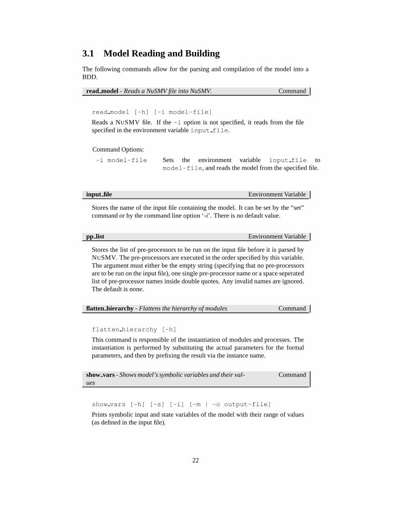
3.1 Model Reading and Building

The following commands allow for the parsing and compilation of the model into aBDD.

read model - Reads a NuSMV file into NuSMV. Command

read model [-h] [-i model-file]

Reads a NUSMV file. If the -i option is not specified, it reads from the filespecified in the environment variable input file.

Command Options:

-i model-file Sets the environment variable input file tomodel-file, and reads the model from the specified file.

input file Environment Variable

Stores the name of the input file containing the model. It can be set by the “set”command or by the command line option ‘-i’. There is no default value.

pp list Environment Variable

Stores the list of pre-processors to be run on the input file before it is parsed byNUSMV. The pre-processors are executed in the order specified by this variable.The argument must either be the empty string (specifying that no pre-processorsare to be run on the input file), one single pre-processor name or a space seperatedlist of pre-processor names inside double quotes. Any invalid names are ignored.The default is none.

flatten hierarchy - Flattens the hierarchy of modules Command

flatten hierarchy [-h]

This command is responsible of the instantiation of modules and processes. Theinstantiation is performed by substituting the actual parameters for the formalparameters, and then by prefixing the result via the instance name.

show vars - Shows model’s symbolic variables and their val-ues

Command

show vars [-h] [-s] [-i] [-m | -o output-file]

Prints symbolic input and state variables of the model with their range of values(as defined in the input file).

22

Command Options:

-s Prints only state variables.-i Prints only input variables.-m Pipes the output to the program specified by the PAGER

shell variable if defined, else through the UNIX command“more”.

-o output-file Writes the output generated by the command tooutput-file.

encode variables - Builds the BDD variables necessary tocompile the model into a BDD.

Command

encode variables [-h] [-i order-file]

Generates the boolean BDD variables and the ADD needed to encode proposi-tionally the (symbolic) variables declared in the model. The variables are createdas default in the order in which they appear in a depth first traversal of the hierar-chy.The input order file can be partial and can contain variables not declared in themodel. Variables not declared in the model are simply discarded. Variables de-clared in the model which are not listed in the ordering input file will be createdand appended at the end of the given ordering list, according to the default order-ing.

Command Options:

-i order-file Sets the environment variable input order file toorder-file, and reads the variable ordering to be usedfrom file order-file. This can be combined with thewrite order command. The variable ordering is writtento a file, which can be inspected and reordered by the user,and then read back in.

input order file Environment Variable

Indicates the file name containing the variable ordering to be used in building themodel by the ‘encode variables’ command. There is no default value.

write order dumps bits Environment Variable

Changes the behaviour of the command write order.

When this variable is set, write order will dump the bits constituting theboolean encoding of each scalar variable, instead of the scalar variable itself.This helps to work at bits level in the variable ordering file. See the commandwrite order for further information. The default value is 0.

write order - Writes variable order to file. Command

23

write order [-h] [-b] [(-o | -f) order-file]

Writes the current order of BDD variables in the file specified via the -o option.If no option is specified the environment variable output order file will beconsidered. If the variable output order file is unset (or set to an emptyvalue) then standard output will be used.

By default, the bits constituting the scalar variables encoding are not dumped.When a variable bit should be dumped, the scalar variable which the bit belongsto is dumped instead if not previously dumped. The result is a variable orderingcontaining only scalar and boolean model variables.

To dump single bits instead of the corresponding scalar variables, either the option-b can be specified, or the environment variable write order dumps bitsmust be previously set.

When the boolean variable dumping is enabled, the single bits will occur withinthe resulting ordering file in the same position that they occur at BDD level.

Command Options:

-b Dumps bits of scalar variables instead of thesingle scalar variables. See also the variablewrite order dumps bits.

-o order-file Sets the environment variable output order file toorder-file and then dumps the ordering list into that file.

-f order-file Alias for the -o option. Supplied for backward compatibil-ity.

output order file Environment Variable

The file where the current variable ordering has to be written. The default valueis ‘temp.ord’.

build model - Compiles the flattened hierarchy into a BDD Command

build model [-h] [-f] [-m Method]

Compiles the flattened hierarchy into a BDD (initial states, invariants, and transi-tion relation) using the method specified in the environment variable partition methodfor building the transition relation.

Command Options:

-m Method Sets the environment variable partition method tothe value Method, and then builds the transition relation.Available methods are Monolithic, Threshold andIwls95CP.

24

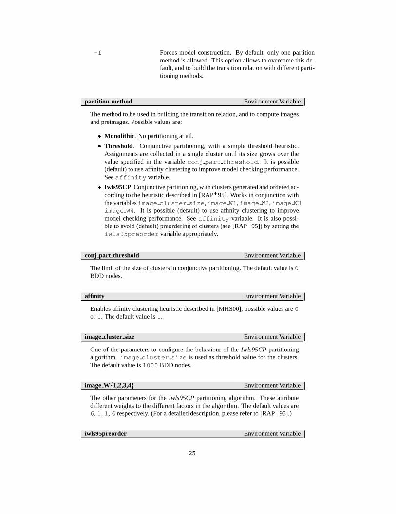
-f Forces model construction. By default, only one partitionmethod is allowed. This option allows to overcome this de-fault, and to build the transition relation with different parti-tioning methods.

partition method Environment Variable

The method to be used in building the transition relation, and to compute imagesand preimages. Possible values are:

� Monolithic. No partitioning at all.� Threshold. Conjunctive partitioning, with a simple threshold heuristic.

Assignments are collected in a single cluster until its size grows over thevalue specified in the variable conj part threshold. It is possible(default) to use affinity clustering to improve model checking performance.See affinity variable.

� Iwls95CP. Conjunctive partitioning, with clusters generated and ordered ac-cording to the heuristic described in [RAP � 95]. Works in conjunction withthe variablesimage cluster size, image W1, image W2, image W3,image W4. It is possible (default) to use affinity clustering to improvemodel checking performance. See affinity variable. It is also possi-ble to avoid (default) preordering of clusters (see [RAP � 95]) by setting theiwls95preorder variable appropriately.

conj part threshold Environment Variable

The limit of the size of clusters in conjunctive partitioning. The default value is 0BDD nodes.

affinity Environment Variable

Enables affinity clustering heuristic described in [MHS00], possible values are 0or 1. The default value is 1.

image cluster size Environment Variable

One of the parameters to configure the behaviour of the Iwls95CP partitioningalgorithm. image cluster size is used as threshold value for the clusters.The default value is 1000 BDD nodes.

image W�1,2,3,4 � Environment Variable

The other parameters for the Iwls95CP partitioning algorithm. These attributedifferent weights to the different factors in the algorithm. The default values are6, 1, 1, 6 respectively. (For a detailed description, please refer to [RAP � 95].)

iwls95preorder Environment Variable

25

Enables cluster preordering following heuristic described in [RAP � 95], possiblevalues are 0 or 1. The default value is 0. Preordering can be very slow.

image verbosity Environment Variable

Sets the verbosity for the image method Iwls95CP, possible values are 0 or 1.The default value is 0.

print iwls95options - Prints the Iwls95 Options. Command

print iwls95options [-h]

This command prints out the configuration parameters of the IWLS95 clusteringalgorithm, i.e. image verbosity, image cluster size and image W

�1,2,3,4 � .

go - Initializes the system for the verification. Command

go [-h]

This command initializes the system for verification. It is equivalent to the com-mand sequenceread model, flatten hierarchy,encode variables,build model, build flat model, build boolean model. If some com-mands have already been executed, then only the remaining ones will be invoked.

process model - Performs the batch steps and then returnscontrol to the interactive shell.

Command

process model [-h] [-i model-file] [-m Method]

Reads the model, compiles it into BDD and performs the model checking of allthe specification contained in it. If the environment variable forward searchhas been set before, then the set of reachable states is computed. If the envi-ronment variables enable reorder and reorder method are set, then thereordering of variables is performed accordingly. This command simulates thebatch behavior of NUSMV and then returns the control to the interactive shell.

Command Options:

-i model-file Sets the environment variable input file tofile model-file, and reads the model from filemodel-file.

-m Method Sets the environment variable partition method toMethod and uses it as partitioning method.

3.2 Commands for Checking Specifications

The following commands allow for the BDD-based model checking of a NUSMVmodel.

26

compute reachable - Computes the set of reachable states Command

compute reachable [-h]

Computes the set of reachable states. The result is then used to simplify im-age and preimage computations. This can result in improved performances formodels with sparse state spaces. Sometimes this option may slow down the per-formances because the computation of reachable states may be very expensive.The environment variable forward search is set during the execution of thiscommand.

print reachable states - Prints out the number of reachablestates

Command

print reachable states [-h] [-v]

Prints the number of reachable states of the given model. In verbose mode, printsalso the list of all reachable states. The reachable states are computed if needed.

check fsm - Checks the transition relation for totality. Command

check fsm [-h] [-m | -o output-file]

Checks if the transition relation is total. If the transition relation is not total thena potential deadlock state is shown.

Command Options:

-m Pipes the output generated by the command to the pro-gram specified by the PAGER shell variable if defined, elsethrough the UNIX command “more”.

-o output-file Writes the output generated by the command to the fileoutput-file.

At the beginning reachable states are computed in order to guarantee that dead-lock states are actually reachable.

check fsm Environment Variable

Controls the activation of the totality check of the transition relation during theprocess model call. Possible values are 0 or 1. Default value is 0.

print fair states - Prints out the number of fair states Command

print fair states [-h] [-v]

27

Prints the number of fair states of the given model. In verbose mode, prints alsothe list of all fair states.

print fair transitions - Prints out the number of fair states Command

print fair transitions [-h] [-v]

Prints the number of fair transitions of the given model. In verbose mode, printsalso the list of all fair transitions. The transitions are displayed as state-inputpairs.

check spec - Performs fair CTL model checking. Command

check spec [-h] [-m | -o output-file] [-n number | -p"ctl-expr [IN context]"]

Performs fair CTL model checking.

A ctl-expr to be checked can be specified at command line using option-p. Alternatively, option -n can be used for checking a particular formula in theproperty database. If neither -n nor -p are used, all the SPEC formulas in thedatabase are checked.

Command Options:

-m Pipes the output generated by the command in processingSPEC s to the program specified by the PAGER shell variableif defined, else through the UNIX command “more”.

-o output-file Writes the output generated by the command in processingSPEC s to the file output-file.

-p "ctl-expr[IN context]"

A CTL formula to be checked. context is the moduleinstance name which the variables in ctl-expr must beevaluated in.

-n number Checks the CTL property with index number in the prop-erty database.

If the ag only search environment variable has been set, then a specializedalgorithm to check AG formulas is used instead of the standard model checkingalgorithms.

ag only search Environment Variable

Enables the use of an ad hoc algorithm for checking AG formulas. Given a for-mula of the form AG alpha, the algorithm computes the set of states satisfyingalpha, and checks whether it contains the set of reachable states. If this is not thecase, the formula is proved to be false.

forward search Environment Variable

28

Enables the computation of the reachable states during the process modelcommand and when used in conjunction with the ag only search environ-ment variable enables the use of an ad hoc algorithm to verify invariants.

check invar - Performs model checking of invariants Command

check invar [-h] [-m | -o output-file] [-n number | -p"invar-expr [IN context]"]

Performs invariant checking on the given model. An invariant is a set of states.Checking the invariant is the process of determining that all states reachable fromthe initial states lie in the invariant. Invariants to be verified can be providedas simple formulas (without any temporal operators) in the input file via theINVARSPEC keyword or directly at command line, using the option -p.

Option -n can be used for checking a particular invariant of the model. If neither-n nor -p are used, all the invariants are checked.

During checking of invariant all the fairness conditions associated with the modelare ignored.

If an invariant does not hold, a proof of failure is demonstrated. This consists ofa path starting from an initial state to a state lying outside the invariant. This pathhas the property that it is the shortest path leading to a state outside the invariant.

Command Options:

-m Pipes the output generated by the program in processingINVARSPEC s to the program specified by the PAGERshell variable if defined, else through the UNIX command“more”.

-o output-file Writes the output generated by the command in processingINVARSPEC s to the file output-file.

-p "invar-expr[IN context]"

The command line specified invariant formula to be verified.context is the module instance name which the variablesin invar-expr must be evaluated in.

check ltlspec - Performs LTL model checking Command

check ltlspec [-h] [-m | -o output-file] [-n number | -p"ltl-expr [IN context]"]

Performs model checking of LTL formulas. LTL model checking is reduced toCTL model checking as described in the paper by [CGH97].

A ltl-expr to be checked can be specified at command line using option-p. Alternatively, option -n can be used for checking a particular formula in theproperty database. If neither -n nor -p are used, all the LTLSPEC formulas inthe database are checked.

Command Options:

29

-m Pipes the output generated by the command in process-ing LTLSPECs to the program specified by the PAGERshell variable if defined, else through the UNIX command“more”.

-o output-file Writes the output generated by the command in processingLTLSPECs to the file output-file.

-p "ltl-expr[IN context]"

An LTL formula to be checked. context is the moduleinstance name which the variables in ltl-expr must beevaluated in.

-n number Checks the LTL property with indexnumber in the propertydatabase.

compute - Performs computation of quantitative character-istics

Command

compute [-h] [-m | -o output-file] [-n number | -p"compute-expr [IN context]"]

This command deals with the computation of quantitative characteristics of realtime systems. It is able to compute the length of the shortest (longest) path fromtwo given set of states.

MAX [ alpha , beta ]MIN [ alpha , beta ]

Properties of the above form can be specified in the input file via the keywordCOMPUTE or directly at command line, using option -p.

Option -n can be used for computing a particular expression in the model. Ifneither -n nor -p are used, all the COMPUTE specifications are computed.

Command Options:

-m Pipes the output generated by the command in process-ing COMPUTEs to the program specified by the PAGERshell variable if defined, else through the UNIX command“more”.

-o output-file Writes the output generated by the command in processingCOMPUTEs to the file output-file.

-p"compute-expr[IN context]"

A COMPUTE formula to be checked. context is the mod-ule instance name which the variables in compute-exprmust be evaluated in.

-n number Computes only the property with index number.

add property - Adds a property to the list of properties Command

add property [-h] [(-c | -l | -i | -q) -p "formula[IN context]"]

30

Adds a property in the list of properties. It is possible to insert LTL, CTL,INVAR and quantitative (COMPUTE) properties. Every newly inserted propertyis initialized to unchecked. A type option must be given to properly execute thecommand.

Command Options:

-c Adds a CTL property.-l Adds an LTL property.-i Adds an INVAR property.-q Adds a quantitative (COMPUTE) property.-p "formula [INcontext]"

Adds the formula specified on the command-line.context is the module instance name which the variablesin formula must be evaluated in.

3.3 Commands for Bounded Model Checking

In this section we describe in detail the commands for doing and controlling BoundedModel Checking in NUSMV. Bounded Model Checking is based on the reduction ofthe bounded model checking problem to a propositional satisfiability problem. Afterthe problem is generated, NUSMV internally calls a propositional SAT solver in or-der to find an assignment which satisfies the problem. Currently NUSMV suppliesthree SAT solvers: SIM, Zchaff and MiniSat. Notice that Zchaff and MiniSat are fornon-commercial purposes only. They are therefore not included in the source codedistribution or in some of the binary distributions of NUSMV.

Some commands for Bounded Model Checking use incremental algorithms. Thesealgorithms exploit the fact that satisfiability problems generated for a particular boundedmodel checking problem often share common subparts. So information obtained dur-ing solving of one satisfiability problem can be used in solving of another one. Theincremental algorithms usually run quicker then non-incremental ones but require aSAT solver with incremental interface. At the moment, only Zchaff and MiniSat offersuch an interface. If none of these solvers are linked to NUSMV, then the commandswhich make use of the incremental algorithms will not be available.

It is also possible to generate the satisfiability problem without calling the SATsolver. Each generated problem is dumped in DIMACS format to a file. DIMACS isthe standard format used as input by most SAT solvers, so it is possible to use NUSMVwith a separate external SAT solver. At the moment, the DIMACS files can be gener-ated only by commands which do not use incremental algorithms.

bmc setup - Builds the model in a Boolean Epression for-mat.

Command

bmc setup [-h]

You must call this command before use any other bmc-related command. Onlyone call per session is required.

go bmc - Initializes the system for the BMC verification. Command

31

go bmc [-h]

This command initializes the system for verification. It is equivalent to the com-mand sequenceread model, flatten hierarchy,encode variables,build boolean model, bmc setup. If some commands have already beenexecuted, then only the remaining ones will be invoked.

check ltlspec bmc - Checks the given LTL specification, orall LTL specifications if no formula is given. Checking pa-rameters are the maximum length and the loopback value

Command

check ltlspec bmc [-h | -n idx | -p "formula [IN context]"][-k max length] [-l loopback] [-o filename]

This command generates one or more problems, and calls SAT solver for eachone. Each problem is related to a specific problem bound, which increases fromzero (

�) to the given maximum problem length. Here max length is the bound

of the problem that system is going to generate and solve. In this context themaximum problem bound is represented by the -k command parameter, or byits default value stored in the environment variable bmc length. The singlegenerated problem also depends on the loopback parameter you can explicitlyspecify by the -l option, or by its default value stored in the environment variablebmc loopback.

The property to be checked may be specified using the -n idx or the -p "formula"options. If you need to generate a DIMACS dump file of all generated problems,you must use the option -o "filename".

Command Options:

-n index index is the numeric index of a valid LTL specification for-mula actually located in the properties database.

-p "formula [INcontext]"

Checks the formula specified on the command-line.context is the module instance name which the variablesin formula must be evaluated in.

-k max length max length is the maximum problem bound to be checked.Only natural numbers are valid values for this option. If novalue is given the environment variable bmc length is con-sidered instead.

-l loopback The loopback value may be:� a natural number in (0, max length-1). A positive sign

(‘+’) can be also used as prefix of the number. Any in-valid combination of length and loopback will be skippedduring the generation/solving process.� a negative number in (-1, -bmc length). In this case loop-back is considered a value relative to max length. Any in-valid combination of length and loopback will be skippedduring the generation/solving process.

32

� the symbol ‘X’, which means “no loopback”.� the symbol ‘*’, which means “all possible loopbacks from

zero to length-1” .-o filename filename is the name of the dumped dimacs file. It may con-

tain special symbols which will be macro-expanded to formthe real file name. Possible symbols are:

� @F: model name with path part.� @f: model name without path part.� @k: current problem bound.� @l: current loopback value.� @n: index of the currently processed formula in the prop-

erty database.� @@: the ‘@’ character.

check ltlspec bmc onepb - Checks the given LTL specifica-tion, or all LTL specifications if no formula is given. Check-ing parameters are the single problem bound and the loop-back value

Command

check ltlspec bmc onepb [-h | -n idx | -p "formula"[IN context]] [-k length] [-l loopback] [-o filename]

As command check ltlspec bmc but it produces only one single problemwith fixed bound and loopback values, with no iteration of the problem boundfrom zero to max length.

Command Options:

-n index index is the numeric index of a valid LTL specification for-mula actually located in the properties database. The validityof index value is checked out by the system.



-k length length is the problem bound used when generating the sin-gle problem. Only natural numbers are valid values forthis option. If no value is given the environment variablebmc length is considered instead.


(’+’) can be also used as prefix of the number. Any in-valid combination of length and loopback will be skippedduring the generation/solving process.� a negative number in (-1, -bmc length). In this case loop-back is considered a value relative to length. Any invalidcombination of length and loopback will be skipped dur-ing the generation/solving process.

33

� the symbol ’X’, which means “no loopback” .� the symbol ’*’, which means “all possible loopback from

zero to length-1”.-o filename filename is the name of the dumped dimacs file. It may con-

tain special symbols which will be macro-expanded to formthe real file name. Possible symbols are:

� @F: model name with path part.� @f: model name without path part.� @k: current problem bound.� @l: current loopback value.� @n: index of the currently processed formula in the prop-

erty database.� @@: the ’@’ character.

gen ltlspec bmc - Dumps into one or more dimacs files thegiven LTL specification, or all LTL specifications if no for-mula is given. Generation and dumping parameters are themaximum bound and the loopback value

Command

gen ltlspec bmc [-h | -n idx | -p "formula" [IN context]][-k max length] [-l loopback] [-o filename]

This command generates one or more problems, and dumps each problem into adimacs file. Each problem is related to a specific problem bound, which increasesfrom zero (0) to the given maximum problem bound. In this short descriptionlength is the bound of the problem that system is going to dump out.

In this context the maximum problem bound is represented by the max length pa-rameter, or by its default value stored in the environment variable bmc length.

Each dumped problem also depends on the loopback you can explicitly spec-ify by the -l option, or by its default value stored in the environment variablebmc loopback.

The property to be checked may be specified using the -n idx or the -p "formula" options.

You may specify dimacs file name by using the option -o filename , other-wise the default value stored in the environment variablebmc dimacs filenamewill be considered.

Command Options:




34

-k max length max length is the maximum problem bound used when in-creasing problem bound starting from zero. Only naturalnumbers are valid values for this option. If no value is giventhe environment variable bmc length value is considered in-stead.


(’+’) can be also used as prefix of the number. Any in-valid combination of bound and loopback will be skippedduring the generation and dumping process.� a negative number in (-1, -bmc length). In this case loop-back is considered a value relative to max length. Any in-valid combination of bound and loopback will be skippedduring the generation process.� the symbol ‘X’, which means “no loopback”.

� the symbol ‘*’, which means “all possible loopback fromzero to length-1”.

-o filename filename is the name of dumped dimacs files. If this optionsis not specified, variable bmc dimacs filename will be con-sidered. The file name string may contain special symbolswhich will be macro-expanded to form the real file name.Possible symbols are:

� @F: model name with path part.� @f: model name without path part.� @k: current problem bound.� @l: current loopback value .� @n: index of the currently processed formula in the prop-

erty database.� @@: the ‘@’ character.

gen ltlspec bmc onepb - Dumps into one dimacs file theproblem generated for the given LTL specification, or for allLTL specifications if no formula is explicitly given. Genera-tion and dumping parameters are the problem bound and theloopback value

Command

gen ltlspec bmc onepb [-h | -n idx | -p "formula"[IN context]] [-k length] [-l loopback] [-o filename]

As the gen ltlspec bmc command, but it generates and dumps only one prob-lem given its bound and loopback.

Command Options:


35



-k length length is the single problem bound used to generate anddump it. Only natural numbers are valid values for thisoption. If no value is given the environment variablebmc length is considered instead.

-l loopback The loopback value may be:� a natural number in (0, length-1). A positive sign (’+’) can

be also used as prefix of the number. Any invalid combi-nation of length and loopback will be skipped during thegeneration and dumping process.� negative number in (-1, -length). Any invalid combinationof length and loopback will be skipped during the gener-ation process.� the symbol ‘X’, which means “no loopback”.

� the symbol ‘*’, which means “all possible loopback fromzero to length-1”.

-o filename filename is the name of the dumped dimacs file. If this op-tions is not specified, variable bmc dimacs filenamewill be considered. The file name string may contain spe-cial symbols which will be macro-expanded to form the realfile name. Possible symbols are:

� @F: model name with path part� @f: model name without path part� @k: current problem bound� @l: current loopback value� @n: index of the currently processed formula in the prop-

erty database� @@: the ’@’ character

check ltlspec bmc inc - Checks the given LTL specification,or all LTL specifications if no formula is given, using an in-cremental algorithm. Checking parameters are the maximumlength and the loopback value

Command

check ltlspec bmc inc [-h | -n idx | -p "formula [IN context]"][-k max length] [-l loopback]

For each problem this command incrementally generates many satisfiability sub-problems and calls the SAT solver on each one of them. The incremental algo-rithm exploits the fact that subproblems have common subparts, so informationobtained during a previous call to the SAT solver can be used in the consecutiveones. Logically, this command does the same thing as check ltlspec bmc(see the description on page 32) but usually runs considerably quicker. A SATsolver with an incremental interface is required by this command, therefore if nosuch SAT solver is provided then this command will be unavailable.

36

Command Options:

-n index index is the numeric index of a valid LTL specification for-mula actually located in the properties database.



-k max length max length is the maximum problem bound must bereached. Only natural numbers are valid values for thisoption. If no value is given the environment variablebmc length is considered instead.


(‘+’) can be also used as prefix of the number. Any in-valid combination of length and loopback will be skippedduring the generation/solving process.� a negative number in (-1, -bmc length). In this case loop-back is considered a value relative to max length. Any in-valid combination of length and loopback will be skippedduring the generation/solving process.� the symbol ‘X’, which means “no loopback”.

� the symbol ‘*’, which means “all possible loopback fromzero to length-1” .

bmc length Environment Variable

Sets the generated problem bound. Possible values are any natural number, butmust be compatible with the current value held by the variable bmc loopback.The default value is 10.

bmc loopback Environment Variable

Sets the generated problem loop. Possible values are:

� Any natural number, but less than the current value of the variable bmc length.In this case the loop point is absolute.

� Any negative number, but greater than or equal to -bmc length. In this casespecified loop is the loop length.

� The symbol ’X’, which means “no loopback”.� The symbol ’*’, which means “any possible loopbacks”.

The default value is *.

bmc dimacs filename Environment Variable

This is the default file name used when generating DIMACS problem dumps.This variable may be taken into account by all commands which belong to thegen ltlspec bmc family. DIMACS file name can contain special symbols whichwill be expanded to represent the actual file name. Possible symbols are:

37

� @F The currently loaded model name with full path.� @f The currently loaded model name without path part.� @n The numerical index of the currently processed formula in the property

database.� @k The currently generated problem length.� @l The currently generated problem loopback value.� @@ The ‘@’ character.

The default value is “@f k@k l@l n@n ”.

check invar bmc - Generates and solves the given invari-ant, or all invariants if no formula is given

Command

check invar bmc [-h | -n idx | -p "formula" [IN context]][-a alg] [-o filename]

In Bounded Model Checking, invariants are proved using induction. For this,satisfiability problems for the base and induction step are generated and a SATsolver is invoked on each of them. At the moment, two algorithms can be used toprove invariants. In one algorithm, which we call “classic”, the base and inductionsteps are built on one state and one transition, respectively. Another algorithm,which we call “een-sorensson” [ES04], can build the base and induction steps onmany states and transitions. As a result, the second algorithm is more powerful.

Command Options:

-n index index is the numeric index of a valid INVAR specificationformula actually located in the property database. The va-lidity of index value is checked out by the system.



-k max length max length is the maximum problem bound that can bereached. Only natural numbers are valid values for this op-tion. Use this option only if the “een-sorensson” algorithmis selected. If no value is given the environment variablebmc length is considered instead.

-a alg alg specifies the algorithm. The value can be classic oreen-sorensson. If no value is given the environmentvariable bmc invar alg is considered instead.

-o filename filename is the name of the dumped dimacs file. It may con-tain special symbols which will be macro-expanded to formthe real file name. Possible symbols are:

� @F: model name with path part� @f: model name without path part� @n: index of the currently processed formula in the prop-

erties database

38

� @@: the ‘@’ character

gen invar bmc - Generates the given invariant, or all in-variants if no formula is given

Command

gen invar bmc [-h | -n idx | -p "formula [IN context]"][-o filename]

At the moment, the invariants are generated using “classic” algorithm only (seethe description of check invar bmc on page 38).

Command Options:




-o filename filename is the name of the dumped dimacs file. If you donot use this option the dimacs file name is taken from theenvironment variable bmc invar dimacs filename.File name may contain special symbols which will be macro-expanded to form the real dimacs file name. Possible sym-bols are:

� @F: model name with path part� @f: model name without path part� @n: index of the currently processed formula in the prop-

erties database� @@: the ’@’ character

check invar bmc inc - Generates and solves the given in-variant, or all invariants if no formula is given, using incre-mental algorithms

Command

check invar bmc inc [-h | -n idx | -p "formula" [IN context]][-a algorithm]

This command does the same thing as check invar bmc (see the descriptionon page 38) but uses an incremental algorithm and therefore usually runs con-siderably quicker. The incremental algorithms exploit the fact that satisfiabilityproblems generated for a particular invariant have common subparts, so informa-tion obtained during solving of one problem can be used in solving another one.A SAT solver with an incremental interface is required by this command. If nosuch SAT solver is provided then this command will be unavailable.

39

There are two incremental algorithms which can be used: “Dual” and “ZigZag”.Both algorithms are equally powerful, but may show different performance de-pending on a SAT solver used and an invariant being proved. At the moment, the“Dual” algorithm cannot be used if there are input variables in a given model. Foradditional information about algorithms, consider [ES04].

Command Options:




-k max length max length is the maximum problem bound that can bereached. Only natural numbers are valid values for thisoption. If no value is given the environment variablebmc length is considered instead.

-a alg alg specifies the algorithm to use. The value can be dualor zigzag. If no value is given the environment variablebmc inc invar alg is considered instead.

bmc invar alg Environment Variable

Sets the default algorithm used by the command check invar bmc. Possiblevalues are classic and een-sorensson. The default value is classic.

bmc inc invar alg Environment Variable

Sets the default algorithm used by the command check invar bmc inc. Pos-sible values are dual and zigzag. The default value is dual.

bmc invar dimacs filename Environment Variable

This is the default file name used when generating DIMACS invar dumps. Thisvariable may be taken into account by the commandgen invar bmc. DIMACSfile name can contain special symbols which will be expanded to represent theactual file name. Possible symbols are:

� @F The currently loaded model name with full path.� @f The currently loaded model name without path part.� @n The numerical index of the currently processed formula in the properties

database.� @@ The ‘@’ character.

The default value is “@f invar n@n ”.

sat solver Environment Variable

40

The SAT solver’s name actually to be used. Default SAT solver is SIM. De-pending on the NUSMV configuration, also the Zchaff and MiniSat SAT solverscan be available or not. Notice that Zchaff and MiniSat are for non-commercialpurposes only.

bmc simulate - Generates a trace of the model from 0 (zero)to k

Command

bmc simulate [-h | -k ]

bmc simulate does not require a specification to build the problem, becauseonly the model is used to build it. The problem length is represented by the -kcommand parameter, or by its default value stored in the environment variablebmc length.

Command Options:

-k length length is the length of the generated simulation.

3.4 Simulation Commands

In this section we describe the commands that allow to simulate a NUSMV specifica-tion. See also the section Section 3.5 [Traces], page 43 that describes the commandsavailable for manipulating traces.

pick state - Picks a state from the set of initial states Command

pick state [-h] [-v] [-r | -i [-a]] [-c "constraints"]

Chooses an element from the set of initial states, and makes it the currentstate (replacing the old one). The chosen state is stored as the first state of anew trace ready to be lengthened by steps states by the simulate command.The state can be chosen according to different policies which can be specified viacommand line options. By default the state is chosen in a deterministic way.

Command Options:

-v Verbosely prints out chosen state (all state variables, oth-erwise it prints out only the label t.1 of the state chosen,where t is the number of the new trace, that is the numberof traces so far generated plus one).

-r Randomly picks a state from the set of initial states.-i Enables the user to interactively pick up an initial state. The

user is requested to choose a state from a list of possibleitems (every item in the list doesn’t show state variables un-changed with respect to a previous item). If the number ofpossible states is too high, then the user has to specify somefurther constraints as “simple expression”.

41

-a Displays all state variables (changed and unchanged with re-spect to a previous item) in an interactive picking. This op-tion works only if the -i options has been specified.

-c"constraints"

Uses constraints to restrict the set of initial states inwhich the state has to be picked. constraints must beenclosed between double quotes " ".

showed states Environment Variable

Controls the maximum number of states showed during an interactive simulationsession. Possible values are integers from 1 to 100. The default value is 25.

simulate - Performs a simulation from the current selectedstate

Command

simulate [-h] [-p | -v] [-r | -i [-a]] [-c "constraints"]steps

Generates a sequence of at most steps states (representing a possible executionof the model), starting from the current state. The current state must be setvia the pick state or goto state commands.

It is possible to run the simulation in three ways (according to different commandline policies): deterministic (the default mode), random and interactive.

The resulting sequence is stored in a trace indexed with an integer number takinginto account the total number of traces stored in the system. There is a differentbehavior in the way traces are built, according to how current state is set: currentstate is always put at the beginning of a new trace (so it will contain at most steps+ 1 states) except when it is the last state of an existent old trace. In this case theold trace is lengthened by at most steps states.

42

Command Options:

-p Prints current generated trace (only those variables whosevalue changed from the previous state).

-v Verbosely prints current generated trace (changed and un-changed state variables).

-r Picks a state from a set of possible future states in a randomway.

-i Enables the user to interactively choose every state of thetrace, step by step. If the number of possible states is toohigh, then the user has to specify some constraints as simpleexpression. These constraints are used only for a single sim-ulation step and are forgotten in the following ones. Theyare to be intended in an opposite way with respect to thoseconstraints eventually entered with the pick state com-mand, or during an interactive simulation session (when thenumber of future states to be displayed is too high), that arelocal only to a single step of the simulation and are forgottenin the next one.

-a Displays all the state variables (changed and unchanged)during every step of an interactive session. This optionworks only if the -i option has been specified.

-c"constraints"

Performs a simulation in which computation is restrictedto states satisfying those constraints. The desired se-quence of states could not exist if such constraints were toostrong or it may happen that at some point of the simulation afuture state satisfying those constraints doesn’t exist: in thatcase a trace with a number of states less than steps trace isobtained. Note: constraints must be enclosed betweendouble quotes " ".

steps Maximum length of the path according to the constraints.The length of a trace could contain less than steps states:this is the case in which simulation stops in an intermediatestep because it may not exist any future state satisfying thoseconstraints.

3.5 Traces

A trace is a sequence of states-inputs pairs corresponding to a possible execution ofthe model. Each pair contains the inputs that caused the transition to the new state,and the new state itself. The initial state has no such input values defined as it doesnot depend on the values of any of the inputs. The values of any constants declared inDEFINE sections are also part of a trace. If the value of a constant depends only onstate variables then it will be treated as if it is a state variable too. If it depends onlyon input variables then it will be treated as if it is an input variable. If however, a con-stant depends upon both input and state variables, then it gets displayed in a seperate“combinatorial” section. Since the values of any such constants depend on one or moreinputs, the initial state does not contain this section either.

43

Traces are created by NUSMV when a formula is found to be false; they are alsogenerated as a result of a simulation (Section 3.4 [Simulation Commands], page 41).Each trace has a number, and the states-inputs pairs are numbered within the trace.Trace n has states/inputs n.1, n.2, n.3, ”...” where n.1 represents the initial state.

3.5.1 Inspecting Traces

The trace inspection commands of NUSMV allow for navigation along the labelledstates-inputs pairs of the traces produced. During the navigation, there is a currentstate, and the current trace is the trace the current state belongs to. The commands arethe following:

goto state - Goes to a given state of a trace Command

goto state [-h] state label

Makes state label the current state. This command is used to navigate alongtraces produced by NUSMV. During the navigation, there is a current state, andthe current trace is the trace the current state belongs to.

print current state - Prints out the current state Command

print current state [-h] [-v]

Prints the name of the current state if defined.

Command Options:

-v Prints the value of all the state variables of the current state.

3.5.2 Displaying Traces

NUSMV comes with three trace plugins (see Section 3.6 [Trace Plugins], page 46)which can be used to display traces in the system. Once a trace has been generated byNUSMV it is printed to stdout using the trace explanation plugin which has beenset as the current default. The command show traces (see Section 3.4 [SimulationCommands], page 41) can then be used to print out one or more traces using a differenttrace plugin, as well as allowing for output to a file.

3.5.3 Trace Plugin Commands

The following commands relate to the plugins which are available in NUSMV.

show plugins - Shows the available trace explanation plug-ins

Command

show plugins [-h] [-n plugin-no | -a]

44

Command Options:

-n plugin-no Shows the plugin with the index number equal toplugin-no.

-a Shows all the available plugins.

Shows the available plugins that can be used to display a trace which has beengenerated by NUSMV, or that has been loaded with the read trace command.The plugin that is used to read in a trace is also shown. The current default pluginis marked with “[D]”.

All the available plugins are displayed by default if no command options aregiven.

default trace plugin Environment Variable

This determines which trace plugin will be used by default when traces that aregenerated by NUSMV are to be shown. The values that this variable can takedepend on which trace plugins are installed. Use the command show pluginsto see which ones are available. The default value is 0.

show traces - Shows the traces generated in a NuSMV ses-sion

Command

show traces [-h] [-v] [-t] [-m | -o output-file] [-p plugin-no][-a | trace number]

Shows the traces currently stored in system memory, if any. By default it showsthe last generated trace, if any.

Command Options:

-v Verbosely prints traces content (all state variables, otherwiseit prints out only those variables that have changed theirvalue from previous state). This option only applies whenthe Basic Trace Explainer plugin is used to display the trace.

-t Prints only the total number of currently stored traces.-a Prints all the currently stored traces.-m Pipes the output through the program specified by the

PAGER shell variable if defined, else through the UNIXcommand “more”.

-o output-file Writes the output generated by the command tooutput-file.

-p plugin-no Uses the specified trace plugin to display the trace.trace number The (ordinal) identifier number of the trace to be printed.

This must be the last argument of the command. Omittingthe trace number causes the most recently generated trace tobe printed.

45

If the XML Format Output plugin is being used to save generated traces to afile with the intent of reading them back in again at a later date, then only onetrace should be saved per file. This is because the trace reader does not currentlysupport multiple traces in one file.

read trace - Loads a previously saved trace Command

read trace [-h | -i file-name]

Command Options:

-i file-name Reads in a trace from the specified file. Note that the filemust only contain one trace.

Loads a trace which has been previously output to a file with the XML FormatOutput plugin. The model from which the trace was originally generated must beloaded and built using the command “go” first.Please note that this command is only available on systems that have the ExpatXML parser library installed.

3.6 Trace Plugins

NUSMV comes with three plugins which can be used to diaplay a trace that has beengenerated:

Basic Trace ExplainerStates/Variables TableXML Format Printer

There is also a plugin which can read in any trace which has been output to a fileby the XML Format Printer. Note however that this reader is only available on systemsthat have the Expat XML parser library installed.

Once a trace has been generated it is output to stdout using the currently selectedplugin. The command show traces can be used to output any previuosly generated,or loaded, trace to a specific file.

3.6.1 Basic Trace Explainer

This plugin prints out each state (the current values of the variables) in the trace, oneafter the other. The initial state contains all the state variables and their initial values.States are numbered in the following fasion:

trace number.state number

46

There is the option of printing out the value of every variable in each state, orjust those which have changed from the previous one. The one that is used can bechosen by selecting the appropriate trace plugin. The values of any constants whichdepend on both input and state variables are printed next. It then prints the set of inputswhich cause the transition to a new state (if the model contains inputs), before actuallyprinting the new state itself. The set of inputs and the subsequent state have the samenumber associated to them.

In the case of a looping trace, if the next state to be printed is the same as the laststate in the trace, a line is printed stating that this is the point where the loop begins.

With the exception of the initial state, for which no input values are printed, theoutput syntax for each state is as follows:

-> Input: TRACE_NO.STATE_NO <-/* for each input var (being printed), i: */INPUT_VARi = VALUE

-> State: TRACE_NO.STATE_NO <-/* for each state var (being printed), j: */STATE_VARj = VALUE/* for each combinatorial constant (being printed), k: */CONSTANTk = VALUE

where INPUT VAR, STATE VAR and CONSTANT have the relevant module namesprepended to them (seperated by a period) with the exception of the module “main” .

The version of this plugin which only prints out those variables whose values havechanged is the initial default plugin used by NUSMV.

3.6.2 States/Variables Table

This trace plugin prints out the trace as a table, either with the states on each row, or ineach column. The entries along the state axis are:

S0 C1 I1 S1 ... Cn In Sn

where S0 is the initial state, and �� gives the values of the input variables whichcaused the transition from state �� to state �� . � gives the values of any combina-torial constants, where the value depends on the values of the state variables in state�� and the values of input variables in state �� .

The variables in the model are placed along the other axis. Only the values of statevariables are displayed in the State row/column, only the values of input variables aredisplayed in the Input row/column and only the values of combinatorial constants aredisplayed in the Constants row/column. All remaining cells have ’-’ displayed.

3.6.3 XML Format Printer

This plugin prints out the trace either to stdout or to a specified file using the com-mand show traces. If traces are to be output to a file with the intention of thembeing loaded again at a later date, then each trace must be saved in a separate file. Thisis because the XML Reader plugin does not currently support multiple traces per file.The format of a dumped XML trace file is as follows:

47

<?XML_VERSION_STRING?><counter-example type=TRACE_TYPE desc=TRACE_DESC>

/* for each state, i: */<node><state id=i>

/* for each state var, j: */<value variable=j>VALUE</value>

</state><combinatorial id=i+1>

/* for each combinatorial constant, k: */<value variable=k>VALUE</value>

</combinatorial><input id=i+1>

/* for each input var, l: */<value variable=l>VALUE</value>

</input></node>

</counter-example>

Note that for the last state in the trace, there is no input section in the node tags.This is because the inputs section gives the new input values which cause the transitionto the next state in the trace. There is also no combinatorial section as this depends onthe values of the inputs and are therefore undefined when there are no inputs.

3.6.4 XML Format Reader

This plugin makes use of the Expat XML parser library and as such can only be used onsystems where this library is available. Previously generated traces for a given modelcan be loaded using this plugin provided that the original model file1 has been loaded,and built using the command go.

When a trace is loaded, it is given the smallest available trace number to identify it.It can then be manipulated in the same way as any generated trace.

3.7 Interface to the DD Package

NUSMV uses the state of the art BDD package CUDD [Som98]. Control over the BDDpackage can very important to tune the performance of the system. In particular, theorder of variables is critical to control the memory and the time required by operations

1To be exact, �� , where �� is the model from which the trace was generated, and �� is thecurrently loaded, and built, model. Note however, that this may mean that the trace is not valid for the model� � .

48

over BDDs. Reordering methods can be activated to determine better variable orders,in order to reduce the size of the existing BDDs.

Reordering of the variables can be triggered in two ways: by the user, or by theBDD package. In the first way, reordering is triggered by the interactive shell commanddynamic var ordering with the -f option.

Reordering is triggered by the BDD package when the number of nodes reaches agiven threshold. The threshold is initialized and automatically adjusted after each re-ordering by the package. This is called dynamic reordering, and can be enabled or dis-abled by the user. Dynamic reordering is enabled with the shell commanddynamic var orderingwith the option -e, and disabled with the -d option.

enable reorder Environment Variable

Specifies whether dynamic reordering is enabled (when value is ‘0’) or disabled(when value is ‘1’).

reorder method Environment Variable

Specifies the ordering method to be used when dynamic variable reordering isfired. The possible values, corresponding to the reordering methods availablewith the CUDD package, are listed below. The default value is sift.

sift: Moves each variable throughout the order to findan optimal position for that variable (assuming allother variables are fixed). This generally achievesgreater size reductions than the window method, butis slower.

random: Pairs of variables are randomly chosen, and swappedin the order. The swap is performed by a series ofswaps of adjacent variables. The best order amongthose obtained by the series of swaps is retained.The number of pairs chosen for swapping equals thenumber of variables in the diagram.

random pivot: Same as random, but the two variables are chosenso that the first is above the variable with the largestnumber of nodes, and the second is below that vari-able. In case there are several variables tied for themaximum number of nodes, the one closest to theroot is used.

sift converge: The sift method is iterated until no further im-provement is obtained.

symmetry sift: This method is an implementation of symmetric sift-ing. It is similar to sifting, with one addition: Vari-ables that become adjacent during sifting are testedfor symmetry. If they are symmetric, they are linkedin a group. Sifting then continues with a group beingmoved, instead of a single variable.

49

symmetry sift converge:The symmetry sift method is iterated until nofurther improvement is obtained.

window�2,3,4 � : Permutes the variables within windows of n adjacent

variables, where n can be either 2, 3 or 4, so as tominimize the overall BDD size.

window�2,3,4 � converge:The window

�2,3,4 � method is iterated until no

further improvement is obtained.group sift: This method is similar to symmetry sift, but

uses more general criteria to create groups.group sift converge:The group siftmethod is iterated until no further

improvement is obtained.annealing: This method is an implementation of simulated an-

nealing for variable ordering. This method is poten-tially very slow.

genetic: This method is an implementation of a genetic algo-rithm for variable ordering. This method is poten-tially very slow.

exact: This method implements a dynamic programmingapproach to exact reordering. It only stores one BDDat a time. Therefore, it is relatively efficient in termsof memory. Compared to other reordering strategies,it is very slow, and is not recommended for more than16 boolean variables.

linear: This method is a combination of sifting and lineartransformations.

linear conv: The linear method is iterated until no further im-provement is obtained.

dynamic var ordering - Deals with the dynamic variableordering.

Command

dynamic var ordering [-d] [-e <method>] [-f <method>] [-h]

Controls the application and the modalities of (dynamic) variable ordering. Dy-namic ordering is a technique to reorder the BDD variables to reduce the sizeof the existing BDDs. When no options are specified, the current status of dy-namic ordering is displayed. At most one of the options -e, -f, and -d shouldbe specified. Dynamic ordering may be time consuming, but can often reducethe size of the BDDs dramatically. A good point to invoke dynamic orderingexplicitly (using the -f option) is after the commands build model, once thetransition relation has been built. It is possible to save the ordering found usingwrite order in order to reuse it (using build model -i order-file)in the future.

Command Options:

-d Disable dynamic ordering from triggering automatically.-e <method> Enable dynamic ordering to trigger automatically whenever

a certain threshold on the overall BDD size is reached.<method> must be one of the following:

50

� sift: Moves each variable throughout the order to find anoptimal position for that variable (assuming all other vari-ables are fixed). This generally achieves greater size re-ductions than the window method, but is slower.� random: Pairs of variables are randomly chosen, andswapped in the order. The swap is performed by a series ofswaps of adjacent variables. The best order among thoseobtained by the series of swaps is retained. The number ofpairs chosen for swapping equals the number of variablesin the diagram.� random pivot: Same as random, but the two variablesare chosen so that the first is above the variable with thelargest number of nodes, and the second is below that vari-able. In case there are several variables tied for the maxi-mum number of nodes, the one closest to the root is used.� sift converge: The sift method is iterated until no furtherimprovement is obtained.� symmetry sift: This method is an implementation ofsymmetric sifting. It is similar to sifting, with one ad-dition: Variables that become adjacent during sifting aretested for symmetry. If they are symmetric, they are linkedin a group. Sifting then continues with a group beingmoved, instead of a single variable.� symmetry sift converge: The symmetry sift method isiterated until no further improvement is obtained.� window

�2,3,4 � : Permutes the variables within windows

of ”n” adjacent variables, where ”n” can be either 2, 3 or4, so as to minimize the overall BDD size.� window

�2,3,4 � converge: The window

�2,3,4 � method

is iterated until no further improvement is obtained.� group sift: This method is similar to symmetry sift, butuses more general criteria to create groups.� group sift converge: The group sift method is iterateduntil no further improvement is obtained.� annealing: This method is an implementation of simu-lated annealing for variable ordering. This method is po-tentially very slow.� genetic: This method is an implementation of a genetic al-gorithm for variable ordering. This method is potentiallyvery slow.� exact: This method implements a dynamic programmingapproach to exact reordering. It only stores a BDD at atime. Therefore, it is relatively efficient in terms of mem-ory. Compared to other reordering strategies, it is veryslow, and is not recommended for more than 16 booleanvariables.

51

� linear: This method is a combination of sifting and lineartransformations.� linear converge: The linear method is iterated until nofurther improvement is obtained.

-f <method> Force dynamic ordering to be invoked immediately. The val-ues for <method> are the same as in option -e.

print bdd stats - Prints out the BDD statistics and parame-ters

Command

print bdd stats [-h]

Prints the statistics for the BDD package. The amount of information depends onthe BDD package configuration established at compilation time. The configurtionparameters are printed out too. More information about statistics and parameterscan be found in the documentation of the CUDD Decision Diagram package.

set bdd parameters - Creates a table with the value of allcurrently active NuSMV flags and change accordingly theconfigurable parameters of the BDD package.

Command

set bdd parameters [-h] [-s]

Applies the variables table of the NUSMV environnement to the BDD pack-age, so the user can set specific BDD parameters to the given value. This com-mand works in conjunction with the print bdd stats and set commands.print bdd stats first prints a report of the parameters and statistics of thecurrent bdd manager. By using the command set, the user may modify the valueof any of the parameters of the underlying BDD package. The way to do it isby setting a value in the variable BDD.parameter name where parametername is the name of the parameter exactly as printed by the print bdd statscommand.

Command Options:

-s Prints the BDD parameter and statistics after the modifica-tion.

3.8 Administration Commands

This section describes the administrative commands offered by the interactive shell ofNUSMV.

! - shell command Command

52

“! ” executes a shell command. The “shell command” is executed by calling“bin/sh -c shell command”. If the command does not exists or you have not theright to execute it, then an error message is printed.

alias - Provides an alias for a command Command

alias [-h] [<name> [<string>]]

The alias command, if given no arguments, will print the definition of all cur-rent aliases. Given a single argument, it will print the definition of that alias (ifany). Given two arguments, the keyword <name> becomes an alias for the com-mand string <string>, replacing any other alias with the same name.

Command Options:

<name> Alias<string> Command string

It is possible to create aliases that take arguments by using the history substitutionmechanism. To protect the history substitution character ‘ %’ from immediate ex-pansion, it must be preceded by a ‘ � ’ when entering the alias.

For example:

NuSMV> alias read "read model -i %:1.smv ; set input order file%:1.ord"NuSMV> read shortwill create an alias ‘read’, execute ”read model -i short.smv; set input order fileshort.ord”. And again:NuSMV> alias echo2 "echo Hi ; echo %* !"NuSMV> echo2 happy birthdaywill print:Hihappy birthday !CAVEAT: Currently there is no check to see if there is a circular dependency inthe alias definition. e.g.NuSMV> alias foo "echo print bdd stats; foo"creates an alias which refers to itself. Executing the command foo will result aninfinite loop during which the command print bdd stats will be executed.

echo - Merely echoes the arguments Command

echo [-h] [-o filename [-a]] <string>

Echoes the specified string either to standard output, or to filename if the op-tion -o is specified.

Command Options:

53

-o filename Echoes to the specified filename instead of to standard out-put. If the option -a is not specified, the file filenamewill be overwritten if it already exists.

-a Appends the output to the file specified by option-o, insteadof overwritting it. Use only with the option -o.

help - Provides on-line information on commands Command

help [-a] [-h] [<command>]

If invoked with no arguments help prints the list of all commands known to thecommand interpreter. If a command name is given, detailed information for thatcommand will be provided.

Command Options:

-a Provides a list of all internal commands, whose names beginwith the underscore character (’ ’) by convention.

history - list previous commands and their event numbers Command

history [-h] [<num>]

Lists previous commands and their event numbers. This is a UNIX-like historymechanism inside the NUSMV shell.

Command Options:

<num> Lists the last <num> events. Lists the last 30 events if<num> is not specified.

History Substitution:The history substitution mechanism is a simpler version of the csh history sub-stitution mechanism. It enables you to reuse words from previously typed com-mands.

The default history substitution character is the ‘%’ (‘!’ is default for shell es-capes, and ‘#’ marks the beginning of a comment). This can be changed usingthe set command. In this description ’%’ is used as the history char. The ‘%’can appear anywhere in a line. A line containing a history substitution is echoedto the screen after the substitution takes place. ‘%’ can be preceded by a ‘ın orderto escape the substitution, for example, to enter a ‘%’ into an alias or to set theprompt.

Each valid line typed at the prompt is saved. If the history variable is set (seehelp page for set), each line is also echoed to the history file. You can use thehistory command to list the previously typed commands.

Substitutions:At any point in a line these history substitutions are available.

54

Command Options:

%:0 Initial word of last command.%:n n-th argument of last command.%$ Last argument of last command.%* All but initial word of last command.%% Last command.%stuf Last command beginning with “stuf”.%n Repeat the n-th command.%-n Repeat the n-th previous command.

�

old�

new Replace “old” with “new” in previous command. Trailingspaces are significant during substitution. Initial spaces arenot significant.

print usage - Prints processor and BDD statistics. Command

print usage [-h]

Prints a formatted dump of processor-specific usage statistics, and BDD usagestatistics. For Berkeley Unix, this includes all of the information in the getrusage()structure.

quit - exits NuSMV Command

quit [-h] [-s]

Stops the program. Does not save the current network before exiting.

Command Options:

-s Frees all the used memory before quitting. This is slower,and it is used for finding memory leaks.

reset - Resets the whole system. Command

reset [-h]

Resets the whole system, in order to read in another model and to perform verifi-cation on it.

set - Sets an environment variable Command

set [-h] [<name>] [<value>]

A variable environment is maintained by the command interpreter. The set com-mand sets a variable to a particular value, and the unset command removes thedefinition of a variable. If set is given no arguments, it prints the current valueof all variables.

55

Command Options:

<name> Variable name<value> Value to be assigned to the variable.

Interpolation of variables is allowed when using the set command. The vari-ables are referred to with the prefix of ’$’. So for example, what follows can bedone to check the value of a set variable:NuSMV> set foo barNuSMV> echo $foobar

The last line “bar” will be the output produced by NUSMV. Variables can be ex-tended by using the character ‘:’ to concatenate values. For example:NuSMV> set foo barNuSMV> set foo $foo:foobarNuSMV> echo $foobar:foobar

The variable foo is extended with the value foobar . Whitespace charactersmay be present within quotes. However, variable interpolation lays the restrictionthat the characters ’:’ and ’/’ may not be used within quotes. This is to allow forrecursive interpolation. So for example, the following is allowedNuSMV> set "foo bar" thisNuSMV> echo $"foo bar"this

The last line will be the output produced by NUSMV.

But in the following, the value of the variable foo/bar will not be interpretedcorrectly: NuSMV> set "foo/bar" thisNuSMV> echo $"foo/bar"foo/bar

If a variable is not set by the set command, then the variable is returned un-changed. Different commands use environment information for different pur-poses. The command interpreter makes use of the following parameters:

56

Command Options:

autoexec Defines a command string to be automatically executed af-ter every command processed by the command interpreter.This is useful for things like timing commands, or tracingthe progress of optimization.

open path “open path” (in analogy to the shell-variable PATH) is a listof colon-separated strings giving directories to be searchedwhenever a file is opened for read. Typically the current di-rectory (.) is the first item in this list. The standard system li-brary (typically NuSMV LIBRARY PATH) is always implic-itly appended to the current path. This provides a convenientshort-hand mechanism for reaching standard library files.

nusmv stderr Standard error (normally ( stderr)) can be re-directed to afile by setting the variable nusmv stderr.

nusmv stdout Standard output (normally ( stdout)) can be re-directed to afile by setting the variable nusmv stdout.

source - Executes a sequence of commands from a file Command

source [-h] [-p] [-s] [-x] <file> [<args>]

Reads and executes commands from a file.

Command Options:

-p Prints a prompt before reading each command.-s Silently ignores an attempt to execute commands from a

nonexistent file.-x Echoes each command before it is executed.<file> File name.

Arguments on the command line after the filename are remembered but not eval-uated. Commands in the script file can then refer to these arguments using thehistory substitution mechanism. EXAMPLE:Contents of test.scr:

read model -i %:2flatten hierarchybuild variablesbuild modelcompute fairness

Typing source test.scr short.smv on the command line will executethe sequence

57

read model -i short.smvflatten hierarchybuild variablesbuild modelcompute fairness

(In this case %:0 gets source, %:1 gets test.scr, and %:2 gets short.smv.)If you type alias st source test.scr and then type st short.smvbozo, you will execute

read model -i bozoflatten hierarchybuild variablesbuild modelcompute fairness

because bozo was the second argument on the last command line typed. In otherwords, command substitution in a script file depends on how the script file wasinvoked. Switches passed to a command are also counted as positional parame-ters. Therefore, if you type st -x short.smv bozo, you will execute

read model -i short.smvflatten hierarchybuild variablesbuild modelcompute fairness

To pass the -x switch (or any other switch) to source when the script usespositional parameters, you may define an alias. For instance, alias srcxsource -x.

See the variable on failure script quits for further information.

time - Provides a simple CPU elapsed time value Command

time [-h]

Prints the processor time used since the last invocation of the time command,and the total processor time used since NUSMV was started.

unalias - Removes the definition of an alias. Command

unalias [-h] <alias-names>

Removes the definition of an alias specified via the alias command.

Command Options:

58

<alias-names> Aliases to be removed

59

unset - Unsets an environment variable Command

unset [-h] <variables>

A variable environment is maintained by the command interpreter. The set com-mand sets a variable to a particular value, and the unset command removes thedefinition of a variable.

Command Options:

<variables> Variables to be unset.

usage - Provides a dump of process statistics Command

usage [-h]

Prints a formatted dump of processor-specific usage statistics. For Berkeley Unix,this includes all of the information in the getrusage() structure.

which - Looks for a file called ”file name” Command

which [-h] <file name>

Looks for a file in a set of directories which includes the current directory as wellas those in the NUSMV path. If it finds the specified file, it reports the found file’spath. The searching path is specified through the set open path command in.nusmvrc.

Command Options:

<file name> File to be searched

3.9 Other Environment Variables

The behavior of the system depends on the value of some environment variables. Forinstance, an environment variable specifies the partitioning method to be used in build-ing the transition relation. The value of environment variables can be inspected andmodified with the “set” command. Environment variables can be either logical or util-ity.

autoexec Environment Variable

Defines a command string to be automatically executed after every commandprocessed by the command interpreter. This may be useful for timing commands,or tracing the progress of optimization.

on failure script quits Environment Variable

60

When a non-fatal error occurs during the interactive mode, the interactive in-terpreter simply stops the currently executed command, prints the reason of theproblem, and prompts for a new command. When set, this variables makes thecommand interpreter quit when an error occur, and then quit NUSMV. This be-haviour might be useful when the command source is controlled by either asystem pipe or a shell script. Under these conditions a mistake within the scriptinterpreted by source or any unexpected error might hang the controlling scriptor pipe, as by default the interpreter would simply give up the current execution,and wait for further commands. The default value of this environment variable is0.

filec Environment Variable

Enables file completion a la “csh”. If the system has been compiled with the“readline” library, the user is able to perform file completion by typing the <TAB>key (in a way similar to the file completion inside the “bash” shell). If the systemhas not been compiled with the “readline” library, a built-in method to performfile completion a la “csh” can be used. This method is enabled with the ‘setfilec’ command. The “csh” file completion method can be also enabled if the“readline” library has been used. In this case the features offered by “readline”will be disabled.

shell char Environment Variable

shell char specifies a character to be used as shell escape. The default valueof this environment variable is ‘!’.

history char Environment Variable

history char specifies a character to be used in history substitutions. Thedefault value of this environment variable is ‘%’.

open path Environment Variable

open path (in analogy to the shell-variable PATH) is a list of colon-separatedstrings giving directories to be searched whenever a file is opened for read. Typ-ically the current directory (.) is first in this list. The standard system library(NuSMV LIBRARY PATH) is always implicitly appended to the current path.This provides a convenient short-hand mechanism for reaching standard libraryfiles.

nusmv stderr Environment Variable

Standard error (normally stderr) can be re-directed to a file by setting the vari-able nusmv stderr.

nusmv stdout Environment Variable

61

reset

goread_model

flatten_hierarchy

build_model

encode_variables

go_bmc

check_ltlspeccheck_invarcheck_trans

check_spec

compute_reachablesimulate

compute_reachable

check_ltlspec_bmcgen_ltlspec_bmccheck_invar_bmcgen_invar_bmcbmc_simulate

Figure 3.1: The dependency among NUSMV commands.

Standard output (normally stdout) can be re-directed to a file by setting theinternal variable nusmv stdout.

nusmv stdin Environment Variable

Standard input (normally stdin) can be re-directed to a file by setting the inter-nal variable nusmv stdin.

62

Chapter 4

Running NuSMV batch

When the -int option is not specified, NUSMV runs as a batch program, in thestyle of SMV, performing (some of) the steps described in previous section in a fixedsequence.

system prompt> NuSMV [command line options] input-file <RET>

The program described in input-file is processed, and the corresponding finite state ma-chine is built. Then, if input-file contains formulas to verify, their truth in the specifiedstructure is evaluated. For each formula which is not true a counterexample is printed.The batch mode can be controlled with the following command line options:

NUSMV [-h | -help] [-v vl] [-int] [-load script file] [-s][-cpp] [-pre pps] [-ofm fm file] [-obm bm file][-lp] [-n idx] [-is] [-ic] [-ils] [-ii][-ctt] [-f] [-r] [-AG] [-coi][-i iv file] [-o ov file] [-reorder] [-dynamic] [-m method][[-mono]|[-thresh cp t]|[-cp cp t]|[-iwls95 cp t]][-noaffinity] [-iwls95preorder][-bmc] [-bmc length k][ input-file]

where the meaning of the options is described below. If input-file is not provided inbatch mode, then the model is read from standard input.

-help-h

Prints the command line help.-v verbose-level

Enables printing of additional information on the internaloperations of NUSMV. Setting verbose-level to 1 gives thebasic information. Using this option makes you feel better,since otherwise the program prints nothing until it finishes,and there is no evidence that it is doing anything at all. Set-ting the verbose-level higher than 1 enables printing of muchextra information.

63

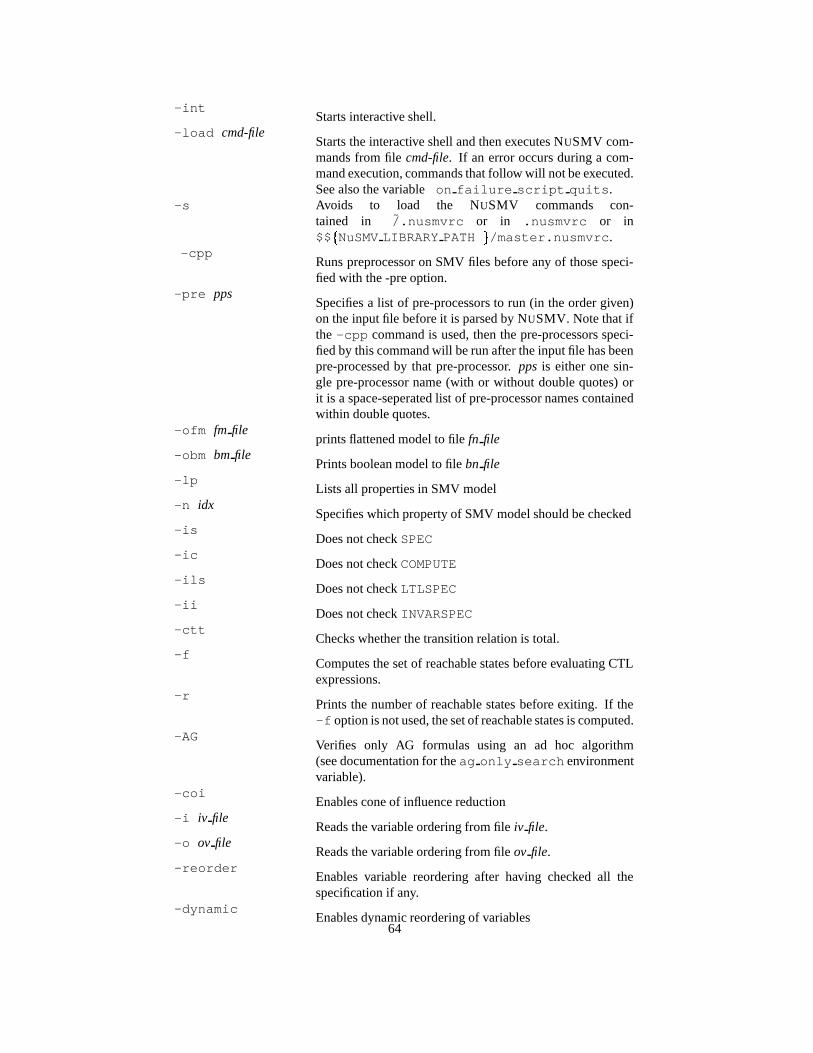
-intStarts interactive shell.

-load cmd-fileStarts the interactive shell and then executes NUSMV com-mands from file cmd-file. If an error occurs during a com-mand execution, commands that follow will not be executed.See also the variable on failure script quits.

-s Avoids to load the NUSMV commands con-tained in /.nusmvrc or in .nusmvrc or in$$

�NuSMV LIBRARY PATH � /master.nusmvrc.

-cppRuns preprocessor on SMV files before any of those speci-fied with the -pre option.

-pre ppsSpecifies a list of pre-processors to run (in the order given)on the input file before it is parsed by NUSMV. Note that ifthe -cpp command is used, then the pre-processors speci-fied by this command will be run after the input file has beenpre-processed by that pre-processor. pps is either one sin-gle pre-processor name (with or without double quotes) orit is a space-seperated list of pre-processor names containedwithin double quotes.

-ofm fm fileprints flattened model to file fn file

-obm bm filePrints boolean model to file bn file

-lpLists all properties in SMV model

-n idxSpecifies which property of SMV model should be checked

-isDoes not check SPEC

-icDoes not check COMPUTE

-ilsDoes not check LTLSPEC

-iiDoes not check INVARSPEC

-cttChecks whether the transition relation is total.

-fComputes the set of reachable states before evaluating CTLexpressions.

-rPrints the number of reachable states before exiting. If the-f option is not used, the set of reachable states is computed.

-AGVerifies only AG formulas using an ad hoc algorithm(see documentation for the ag only search environmentvariable).

-coiEnables cone of influence reduction

-i iv fileReads the variable ordering from file iv file.

-o ov fileReads the variable ordering from file ov file.

-reorderEnables variable reordering after having checked all thespecification if any.

-dynamicEnables dynamic reordering of variables

64

-m methodUses method when variable ordering is enabled. Pos-sible values for method are those allowed for thereorder method environment variable (see Section 3.7[Interface to DD package], page 48).

-monoEnables monolithic transition relation

-thresh cp tconjunctive partitioning with threshold of each partition setto cp t (DEFAULT, with cp t=1000)

-cp cp tDEPRECATED: use thresh instead.

-iwls95 cp tEnables Iwls95 conjunctive partitioning and sets the thresh-old of each partition to cp t

-noaffinityDisables affinity clustering

-iwls95preoderEnables Iwls95CP preordering

-bmcEnables BMC instead of BDD model checking

-bmc kSets bmc length variable, used by BMC

65

Bibliography

[BCCZ99] A. Biere, A. Cimatti, E. Clarke, and Y. Zhu. Symbolic model checkingwithout bdds. In Tools and Algorithms for Construction and Analysis ofSystems, In TACAS’99, March 1999.

[BCL � 94] J.R. Burch, E.M. Clarke, D.E. Long, K.L. McMillan, and D.L. Dill. Sym-bolic model checking for sequential circuit verification. In IEEE Trans-actions on Computer-Aided Design of Integrated Circuits and Systems,13(4):401–424, April 1994.

[CBM90] O. Coudert, C. Berthet, and J. C. Madre. Verification of synchronoussequential machines based on symbolic execution. In In J. Sifakis, edi-tor, Proceedings of the International Workshop on Automatic VerificationMethods for Finite State Systems, volume 407 of LNCS, pages 365–373,Berlin, June 1990.

[CCG � 02] A. Cimatti, E. Clarke, E. Giunchiglia, F. Giunchiglia, M. Pistore,M. Roveri, R. Sebastiani, and A. Tacchella. Nusmv 2: An opensourcetool for symbolic model checking. In Proceedings of Computer Aided Ver-ification (CAV 02), 2002.

[CCGR00] A. Cimatti, E. Clarke, F. Giunchiglia, and M. Roveri. Nusmv: a newsymbolic model checker. In International Journal on Software Tools forTechnology Transfer (STTT), 2(4), March 2000.

[CGH97] E. Clarke, O. Grumberg, and K. Hamaguchi. Another look at ltl modelchecking. In Formal Methods in System Design, 10(1):57–71, February1997.

[Dil88] D. Dill. Trace theory for automatic hierarchical verification of speed-independent circuits. In ACM Distinguished Dissertations. MIT Press,1988.

[EMSS91] E. Allen Emerson, A. K. Mok, A. Prasad Sistla, and Jai Srinivasan. Quan-titative temporal reasoning. In Edmund M. Clarke and Robert P. Krushan,editors, Proceedings of Computer-Aided Verification (CAV’90), volume531 of LNCS, pages 136-145, Berlin, Germany, June 1991.

[ES04] Niklas Een and Niklas Sorensson. Temporal induction by incremental satsolving. In Ofer Strichman and Armin Biere, editors, Electronic Notes inTheoretical Computer Science, volume 89. Elsevier, 2004.

66

[Mar85] A.J. Martin. The design of a self-timed circuit for distributed mutual ex-clusion. In In H. Fuchs and W.H. Freeman, editors, Proceedings of the1985 Chapel Hill Conference on VLSI, pages 245–260, New York, 1985.

[McM92] K.L. McMillan. The smv system – draft. In Available athttp://www.cs.cmu.edu/ modelcheck/smv/smvmanual.r2.2.ps,1992.

[McM93] K.L. McMillan. Symbolic model checking. In Kluwer Academic Publ.,1993.

[MHS00] Moon, Hachtel, and Somenzi. Border-block tringular form and conjunc-tion schedule in image computation. In FMCAD, 2000.

[RAP � 95] R. K. Ranjan, A. Aziz, B. Plessier, C. Pixley, and R. K. Brayton. Effi-cient bdd algorithms for fsm synthesis and verification. In In IEEE/ACMProceedings International Workshop on Logic Synthesis, Lake Tahoe (NV),May 1995.

[sfVS96] ”VIS: A system for Verification and The VIS Group Synthesis”. Proceed-ings of the 8th international conference on computer aided verification,p428-432. In Springer Lecture Notes in Computer Science, 1102, Editedby R. Alur and T. Henzinger, New Brunswick, NJ, 1996.

[Som98] F. Somenzi. Cudd: Cu decision diagram package — release 2.2.0. InDepartment of Electrical and Computer Engineering — University of Col-orado at Boulder, May 1998.

67

Appendix A

Compatibility with CMU SMV

The NUSMV language is mostly source compatible with the original version of SMVdistributed at Carnegie Mellon University from which we started. In this appendix wedescribe the most common problems that can be encountered when trying to use oldCMU SMV programs with NUSMV.

The main problem is variable names in old programs that conflicts with new re-served words. The list of the new reserved words of NUSMV w.r.t. CMU SMV is thefollowing:

F, G, X, U, V,W, H, O, Y, Z,S, T, B

These names are reserved for the LTL temporal operators.

LTLSPEC It is used to introduce LTL specifications.INVARSPEC It is used to introduce invariant specifications.IVAR It is used to introduce input variables.JUSTICE It is used to introduce “justice” fairness constraints.COMPASSION It is used to introduce “compassion” fairness constraints.

The IMPLEMENTS, INPUT, OUTPUT statements are not supported by NUSMV.They are parsed from the input file, but are internally ignored.

NUSMV differs from CMU SMV also in the controls that are performed on theinput formulas. Several formulas that are valid for CMU SMV, but that have no clearsemantics, are not accepted by NUSMV. In particular:

� It is no longer possible to write formulas containing nested ‘next’.

TRANSnext(alpha & next(beta | next(gamma))) -> delta

� It is no longer possible to write formulas containing ‘next’ in the right handside of “normal” and “init” assignments (they are allowed in the right hand sideof “next” assignments), and with the statements ‘INVAR’ and ‘INIT’.

INVARnext(alpha) & beta

INITnext(beta) -> alpha

68

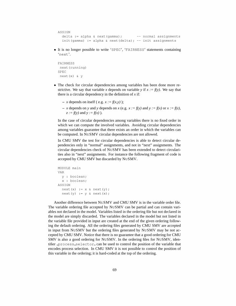
ASSIGNdelta := alpha & next(gamma); -- normal assignmentsinit(gamma) := alpha & next(delta); -- init assignments

� It is no longer possible to write ‘SPEC’, ‘FAIRNESS’ statements containing‘next’.

FAIRNESSnext(running)SPECnext(x) & y

� The check for circular dependencies among variables has been done more re-strictive. We say that variable x depends on variable y if x := f(y). We say thatthere is a circular dependency in the definition of x if:

– x depends on itself ( e.g. x := f(x,y) );

– x depends on y and y depends on x (e.g. x := f(y) and y := f(x) or x := f(z),z := f(y) and y := f(x) ).

In the case of circular dependencies among variables there is no fixed order inwhich we can compute the involved variables. Avoiding circular dependenciesamong variables guarantee that there exists an order in which the variables canbe computed. In NUSMV circular dependencies are not allowed.

In CMU SMV the test for circular dependencies is able to detect circular de-pendencies only in “normal” assignments, and not in “next” assignments. Thecircular dependencies check of NUSMV has been extended to detect circulari-ties also in “next” assignments. For instance the following fragment of code isaccepted by CMU SMV but discarded by NUSMV.

MODULE mainVARy : boolean;x : boolean;

ASSIGNnext(x) := x & next(y);next(y) := y & next(x);

Another difference between NUSMV and CMU SMV is in the variable order file.The variable ordering file accepted by NUSMV can be partial and can contain vari-ables not declared in the model. Variables listed in the ordering file but not declared inthe model are simply discarded. The variables declared in the model but not listed inthe variable file provided in input are created at the end of the given ordering follow-ing the default ordering. All the ordering files generated by CMU SMV are acceptedin input from NUSMV but the ordering files generated by NUSMV may be not ac-cepted by CMU SMV. Notice that there is no guarantee that a good ordering for CMUSMV is also a good ordering for NUSMV. In the ordering files for NUSMV, iden-tifier process selector can be used to control the position of the variable thatencodes process selection. In CMU SMV it is not possible to control the position ofthis variable in the ordering; it is hard-coded at the top of the ordering.

69

Command Index

!, see bang 52

, 52add property, 30alias, 53bmc setup, 31bmc simulate, 41build model, 24check fsm, 27check invar bmc inc, 39check invar bmc, 38check invar, 29check ltlspec bmc inc, 36check ltlspec bmc onepb, 33check ltlspec bmc, 32check ltlspec, 29check spec, 28compute reachable, 27compute, 30dynamic var ordering, 50echo, 53encode variables, 23flatten hierarchy, 22gen invar bmc, 39gen ltlspec bmc onepb, 35gen ltlspec bmc, 34go bmc, 31goto state, 44go, 26help, 54history, 54pick state, 41print bdd stats, 52print current state, 44print fair states, 27print fair transitions, 28print iwls95options, 26print reachable states, 27print usage, 55process model, 26

quit, 55read model, 22read trace, 46reset, 55set bdd parameters, 52set, 55show plugins, 44show traces, 45show vars, 22simulate, 42source, 57time, 58unalias, 58unset, 60usage, 60which, 60write order, 23

70

Variable Index

NuSMV LIBRARY PATH, 61, 64affinity, 25ag only search, 28autoexec, 60bmc dimacs filename, 37bmc inc invar alg, 40bmc invar alg, 40bmc invar dimacs filename, 40bmc length, 37bmc loopback, 37check fsm, 27conj part threshold, 25default trace plugin, 45enable reorder, 49filec, 61forward search, 29history char, 61image W

�1,2,3,4 � , 25

image cluster size, 25image verbosity, 26input file, 22input order file, 23iwls95preorder, 26nusmv stderr, 61nusmv stdin, 62nusmv stdout, 62on failure script quits, 61open path, 61output order file, 24partition method, 25pp list, 22reorder method, 49sat solver, 41shell char, 61showed states, 42verbose level, 21write order dumps bits, 23

71

Index

Symbols.nusmvrc, 64-AG, 64-bmc, 65-bmc k, 65-coi, 64-cpp, 64-cp cp t, 65-ctt, 64-dynamic, 64-f, 64-help, 63-h, 63-ic, 64-ii, 64-ils, 64-int, 64-is, 64-iwls95preorder, 65-iwls95 cp t, 65-i iv file, 64-load cmd-file, 64-lp, 64-mono, 65-m method, 65-noaffinity, 65-n idx, 64-obm bm file, 64-ofm fm file, 64-o ov file, 64-pre pps, 64-reorder, 64-r, 64-thresh cp t, 65-v verbose-level, 63FAIRNESS declarations, 14IVAR declaration, 9VAR declaration, 9running, 14temp.ord, 24

/.nusmvrc, 64

Aadministration commands, 52Array Variables, 20

BBasic Trace Explainer, 46batch, running NUSMV, 63

Ccase expressions, 7Commands for Bounded Model Check-

ing, 31comments in NUSMV language, 6compassion constraints, 14CTL Specifications, 15

DDD package interface, 48DEFINE declarations, 11Displaying Traces, 44

Eexpressions, 6

Ffair execution paths, 14fairness constraints, 14fairness constraints declaration, 14fair paths, 14

IIdentifiers, 13infinity, 18INIT declaration, 10Input File Syntax, 18input variables syntax, 9Inspecting Traces, 44interactive, running NUSMV, 21interactive shell, 21

72

interface to DD Package, 48INVAR declaration, 11ISA declarations, 11

Jjustice constraints, 14

LLTL Specifications, 16

Mmain module, 14master.nusmvrc, 64model compiling, 22model parsing, 22model reading, 22MODULE declarations, 12

NNext Expressions, 8next expressions, 8

Ooptions, 63

Pprocess, 14processes, 14process keyword, 14

RReal Time CTL Specifications and Com-

putations, 17

SScalar Variables, 19self, 13set expressions, 7Shell configuration Variables, 60simple expressions, 6Simulation Commands, 41States/Variables Table, 47state variables syntax, 9

TTrace Plugin Commands, 44Trace Plugins, 46Traces, 43TRANS declarations, 10type declaration, 9type specifiers, 9

Vvar id, 7

XXML Format Printer, 47XML Format Reader, 48

73

nusmv 2.2 user manualnusmv.fbk.eu/nusmv/userman/v22/nusmv.pdf · emanuele olivetti, gavin keighren,...

Documents