NUREG/CR-6785 ANL-01/22

Evaluation of Eddy CurrentReliability from Steam Generator Mock-Up Round-Robin

Argonne National Laboratory

U.S. Nuclear Regulatory Commission Office of Nuclear Regulatory Research Washington, DC 20555-0001

AVAILABILITY OF REFERENCE MATERIALS IN NRC PUBLICATIONS

NRC Reference Material

As of November 1999, you may electronically access NUREG-series publications and other NRC records at NRC's Public Electronic Reading Room at http //www.nrc aov/readn-q-rm html Publicly released records include, to name a few, NUREG-series publications; Federal Register notices; applicant, licensee, and vendor documents and correspondence; NRC correspondence and internal memoranda; bulletins and information notices; inspection and investigative reports; licensee event reports; and Commission papers and their attachments.

NRC publications in the NUREG series, NRC regulations, and Title 10, Energy, in the Code of Federal Regulations may also be purchased from one of these two sources. 1. The Superintendent of Documents

U.S. Government Printing Office Mail Stop SSOP Washington, DC 20402-0001 Internet: bookstore gpo.gov Telephone: 202-512-1800 Fax: 202-512-2250

2. The National Technical Information Service Springfield, VA 22161-0002 www.ntis.gov 1-800-553-6847 or, locally, 703-605-6000

A single copy of each NRC draft report for comment is available free, to the extent of supply, upon written request as follows: Address: Office of the Chief Information Officer,

Reproduction and Distribution Services Section

U.S. Nuclear Regulatory Commission Washington, DC 20555-0001

E-mail: DISTRIBUTION@nrc.gov Facsimile: 301-415-2289

Some publications in the NUREG series that are posted at NRC's Web site address http Ilwww nrc .qovlreadinp-rm/doc-collectionslnuregs are updated periodically and may differ from the last printed version. Although references to material found on a Web site bear the date the material was accessed, the material available on the date cited may subsequently be removed from the site.

Non-NRC Reference Material

Documents available from public and special technical libraries include all open literature items, such as books, journal articles, and transactions, Federal Register notices, Federal and State legislation, and congressional reports. Such documents as theses, dissertations, foreign reports and translations, and nonNRC conference proceedings may be purchased from their sponsoring organization.

Copies of industry codes and standards used in a substantive manner in the NRC regulatory process are maintained at

The NRC Technical Library Two White Flint North 11545 Rockville Pike Rockville, MD 20852-2738

These standards are available in the library for reference use by the public. Codes and standards are usually copyrighted and may be purchased from the originating organization or, if they are American National Standards, from

American National Standards Institute 11 West 42nd Street New York, NY 10036-8002 www.ansi.org 212-642-4900

Legally binding regulatory requirements are stated only in laws; NRC regulations; licenses, including technical specifications; or orders, not in NUREG-series publications. The views expressed in contractor-prepared publications in this series are not necessarily those of the NRC.

The NUREG series comprises (1) technical and administrative reports and books prepared by the staff (NUREG-XXXX) or agency contractors (NUREG/CR-XXXX), (2) proceedings of conferences (NUREG/CP-XXXX), (3) reports resulting from international agreements (NUREGIIA-XXXX), (4) brochures (NUREG/BR-XXXX), and (5) compilations of legal decisions and orders of the Commission and Atomic and Safety Licensing Boards and of Directors' decisions under Section 2.206 of NRC's regulations (NUREG-0750).

DISCLAIMER: This publication was prepared with the support of the U.S. Nuclear Regulatory Commission (NRC) Grant Program. This program supports basic, advanced, and developmental scientific research for a public purpose in areas related to nuclear safety. The grantee bears prime responsibility for the conduct of the research and exercises judgement and original thought toward attaining the scientific goals. The opinions, findings, conclusions, and recommendations expressed herein are therefore those of the authors and do not necessarily reflect the views of the NRC.

NUREG/CR-6785 ANL-01/22

Evaluation of Eddy Current Reliability from Steam Generator Mock-Up Round-Robin

Manuscript Completed: November 2001 Date Published: September 2002

Prepared by D. S. Kupperman, S. Bakhtiari, W. J. Shack, J. Y. Park, S. Majumdar

Argonne National Laboratory 9700 South Cass Avenue Argonne, IL 60439

J. Davis, NRC Project Manager

Prepared for Division of Engineering Technology

Office of Nuclear Regulatory Research

U.S. Nuclear Regulatory Commission

Washington, DC 20555-0001

NRC Job Code W6487

NUREG/CR-6785, has been reproduced from the best available copy.

For sale by the Superntendent of Documents, U S Government Prnting Office Internet bookstore gpo gov Phone toll free (866) 512-1800; DC area (202) 512-1800

Fax (202) 512-2250 Mail Stop SSOP, Washington, DC 20402-0001

ISBN 0-16-051217-4

Evaluation of Eddy Current Reliability from Steam Generator Mock-Up Round-Robin

By

D. S. Kupperman, S. Bakhtiari, W. J. Shack, J. Y. Park and S. Majumdar

Abstract

This report presents an independent assessment of steam generator (SG) inspection reliability that was developed through a nondestructive evaluation round-robin on a steam generator mock-up at Argonne National Laboratory (ANL). The report does not establish regulatory position. The purpose of the round-robin was to assess the current state of SG tubing in-service inspection reliability, determine the probability of detection (POD) as function of flaw size or severity, and to assess the capability for sizing of flaws. Eleven teams participated in analyzing bobbin and rotating coil mock-up data collected by qualified industry personnel. The mock-up contains hundreds of cracks and simulations of artifacts such as corrosion deposits and tube support plates that make detection and characterization of cracks more difficult in operating steam generators than in most laboratory situations. An expert Task Group from industry, Argonne National Laboratory, and the NRC have reviewed the signals from the laboratorygrown cracks used in the mock-up to ensure that they provide reasonable simulations of those obtained in the field. The number of tubes inspected and the number of teams participating in the round-robin are intended to provide better statistical data on the POD and characterization accuracy than is currently available EPRI qualification programs.

iii

Contents Executive Summ ary ..................................................................................................................... xi

Acknowledgments ....................................................................................................................... xiv

Acronym s and Abbreviations ....................................................................................................... xv

I Introduction ........................................................................................................................ 1

2 Program Description .......................................................................................................... 3

2.1 Steam Generator M ock-Up Facility ............................................................................ 3 2.1.1 Equivalencies ................................................................................................... 7 2.1.2 Standards ......................................................................................................... 8 2.1.3 Flaw Fabrication and M orphology ..................................................................... 10

2.1.3.1 Justification for Selection of Flaw Types ................................................ 10 2.1.3.2 Process for Fabricating Cracks ............................................................... 12 2.1.3.3 M atrix of Flaws .................................................................................... 12 2.1.3.4 Crack Profiles by Advanced Multiparameter Algorithm

and Comparison to Fractography ........................................................... 13 2.1.3.4.1 Procedures for Collecting Data

for M ultiparameter Analysis .................................................. 15 2.1.3.4.2 Fractography Procedures ........................................................ 16 2.1.3.4.3 Procedure for Comparing Multiparameter Results

to Fractography ..................................................................... 16 2.1.3.4.4 Multiparameter Profiles vs. Fractography

for Laboratory Samples ......................................................... 17 2.1.3.4.5 Characterization of Cracks in Term s of mp .............................. 27

2.1.3.5 Summary of Sizing Accuracy ............................................................... 30 2.1.3.6 Reference State Table Summary for M ock-up ........................................ 33

2.2 Design and Organization of Round-Robin ................................................................. 33 2.2.1 The M ock-Up as ANL's Steam Generator .......................................................... 33

2.2.1.1 Responsibilities .................................................................................... 37 2.2.1.1.1 Data Collection ...................................................................... 37 2.2.1.1.2 NDE Task Group ................................................................... 37 2.2.1.1.3 Analysis of Round-Robin ....................................................... 37 2.2.1.1.4 Statistical Analysis ............................................................... 37 2.2.1.1.5 Documentation ..................................................................... 37

2.2.2 Round-Robin Documentation ............................................................................ 38 2.2.2.1 Degradation Assessment (ANL003 Rev. 3) ............................................ 38 2.2.2.2 Data Acquisition Documentation (ANL002 Rev. 3) ................................ 39 2.2.2.3 ANL Analysis Guideline (ANL001 Rev. 3) ............................................ 40 2.2.2.4 Training M anual (ANLOO4 Rev. 3) ........................................................ 41 2.2.2.5 Examination Technique Specification Sheet (ETSS) ............................... 41

2.2.3 Acquisition of Eddy Current Mock-Up Data and Description of Data Acquisition Documentation ............................................................................... 42

2.2.4 Examination Technique Specification Sheets ...................................................... 44 2.2.5 Participating Companies and Organization of Team Members ............................ 44 2.2.6 Review of Training M anual by Teams ............................................................... 56 2.2.7 Sequence of Events during Round-Robin Exercise ............................................. 56

v

2.2.8 Data Analysis Procedures and Guidelines ......................................................... 57 2.3 Comparison of Round-Robin Data Acquisition and Analysis to Field ISI ...................... 58 2.4 Strategy for Evaluation of Results .............................................................................. 65

2.4.1 General Principles ............................................................................................ 65 2.4.2 Tolerance for Errors in Location ........................................................................ 65 2.4.3 Handling of False Calls .................................................................................... 65 2.4.4 Procedures for Determining POD ...................................................................... 66

2.4.4.1 Converting SSPD Result to Text Files and Excel Files ............................ 68 2.5 Statistical Analysis .................................................................................................... 68

2.5.1 Determination of Logistic Fits ........................................................................... 68 2.5.2 Uncertainties in the POD Curves ....................................................................... 70 2.5.3 Significance of Difference between Two POD Curves ........................................ 73

2.6 Results of Analysis Round-Robin ............................................................................... 74 2.6.1 POD Logistic Fits with 95% Lower Confidence Bounds ..................................... 74

2.6.1.1 Bobbin Coil Results .............................................................................. 74 2.6.1.2 M RPC Tube Sheet Results ................................................................... 82 2.6.1.3 M RPC Special Interest Results .............................................................. 87

2.7 Nature of M issed Flaws ............................................................................................. 87 2.8 Nature of Overcalls ................................................................................................... 89

3 Summary ........................................................................................................................... 90

3.1 Bobbin Coil Results .................................................................................................. 90 3.2 Tube Sheet M RPC Results ......................................................................................... 91 3.3 M RPC Analysis of TSP Signals ................................................................................ 91 3.4 Accuracy of M aximum Depth for M ock-Up Cracks ................................................... 92 3.5 Overall Capability ..................................................................................................... 92

References .................................................................................................................................. 94

vi

I

Figures

2.1 Schematic representation of steam generator mock-up tube bundle ........................................ 4 2.2 Photograph of m ock-up during acquisition of eddy current data ............................................ 5 2.3 Photograph of sludge on a tube sheet test section ................................................................. 7 2.4 Photograph of dent in a test section ..................................................................................... 7 2.5 Isometric plot (c-scan) showing eddy current response from 400-am-wide

by 250-jim-thick by 25-mm-long, axially oriented magnetite filled epoxy marker located on ID side at end of 22.2 m m (0.875-in.) Inconel 600 tube ........................................ 8

2.6 Bobbin coil voltage histogram for m ock-up flaws and conditions .......................................... 9 2.7 Bobbin coil voltage histogram for m ock-up flaws ................................................................ 9 2.8 Comparison of bobbin coil voltage and phase for representative cracks in mock-up

and M cGuire field data ...................................................................................................... . 9 2.9 Schematic drawing showing configuration of stand, standards, and degraded test

section during an eddy current inspection of a single test section ........................................... 10 2.10 Schematic drawing of ASME and 18-notch standard used when scanning degraded test

sections and mock-up tubes ............................................................................................... 11 2.11 Inscribed identification of tube specimen ............................................................................. 13 2.12 Dye penetration examination of tube specimen SGL865 showing an LODSCC ...................... 13 2.13 Cross-sectional optical metallography: (a) branched LODSCC; (b) LODSCC ........................ 14 2.14 Sketch of dye penetrant images of three ODSCCs in m ock-up .............................................. 14 2.15 Fractography of tube specimen SGL413 ............................................................................. 16 2.16 Sizes and shapes of LODSCCs in tube specimen AGL 536 determined by EC NDE

using the m ultiparameter algorithm and fractography ........................................................... 17 2.17 AGL 2241 CODSSC .......................................................................................................... 18 2.18 AGL 2242 CIDSSC ........................................................................................................... 18 2.19 AGL 288 LIDSCC ............................................................................................................. 18 2.20 AGL 394 CODSCC ........................................................................................................... 19 2.21 AGL 533 LODSCC .......................................................................................................... 19 2.22 AGL 535 LODSCC ........................................................................................................... 19 2.23 AGL 536 LODSCC ........................................................................................................... 20 2.24 AGL 503 LODSCC ........................................................................................................... 20 2.25 AGL 516 LODSCC ........................................................................................................... 20 2.26 AGL 517 LODSCC ........................................................................................................... 21 2.27 AGL 824 LODSCC ........................................................................................................... 21 2.28 AGL 826 CODSCC ........................................................................................................... 21 2.29 AGL 835 LODSCC .......................................................................................................... 22 2.30 AGL 838 CODSCC ........................................................................................................... 22 2.31 AGL 854 LODSCC .......................................................................................................... 22 2.32 AGL 855 LODSCC ........................................................................................................... 23 2.33 AGL 861 LODSCC .......................................................................................................... 23 2.34 AGL 874 LODSCC ........................................................................................................... 23 2.35 AGL 876 LODSCC ........................................................................................................... 24 2.36 AGL 883 LODSCC ........................................................................................................... 24 2.37 AGL 893 CODSCC ........................................................................................................... 24 2.38 AGL 8161LIDSCC ........................................................................................................... 25 2.39 AGL 8162 LIDSCC ........................................................................................................... 25

vii

2.40 Comparison of maximum depth determined by the multiparameter algorithm with that determ ined by fractography .................................................................................. 25

2.41 Comparison of depths determined by the multiparameter algorithm with those by fractography and regression fit and estimated 95% bounds for the observed depth as a function of the multiparameter depth estimate ............................................................... 26

2.42 Comparison of depths determined by the multiparameter algorithm with those by fractography ................................................................................................................. 26

2.43 Maximum eddy current depth as percent throughwall using a pancake coil and multiparameter algorithm for 10 LODSCC and CODSCC from a 20-test-section set vs. destructive analysis result .............................................................................................. 27

2.44 Estimates of crack depths by the multiparameter algorithm compared with estimates of maximum crack depth using +Point phase analysis at 300 kHz ......................................... 28

2.45 Maximum bobbin coil voltage as a function of maximum crack depth for mock-up FS and T SP SC C .................................................................................................................... 28

2.46 Bobbin coil phase angle as a function of maximum crack depth for mock-up TSP L O D SC C .......................................................................................................................... 28

2.47 Bobbin coil phase angle as a function of maximum crack depth for mock-up TSP L ID SC C ............................................................................................................................ 29

2.48 Crack depth profile measured by eddy current and a candidate equivalent rectangular crack corresponding to depth do = 50% and Lo = 10 mm ..................................................... 31

2.49 Ligament rupture pressures corresponding to three candidate equivalent rectangular cracks, 11 mm by 60%, 9 mm by 70%, and 7 mm by 75% .................................................... 31

2.50 Standard deviation in percent throughwall as a function of maximum depth .......................... 32 2.51 Photograph of underside of tube bundle ............................................................................... 43 2.52 Isometric plot of mock-up tubesheet level roll transition from data collected

by rotating +Point coil at 300 kHz (example 1) .................................................................... 59 2.53 Isometric plot of mock-up tubesheet level roll transition from data collected

by rotating +Point coil at 300 kHz (example 2) .................................................................... 59 2.54 Isometric plot of mock-up tubesheet level roll transition from data collected

by rotating +Point coil at 300 kHz (example 3) .................................................................... 60 2.55 Isometric plot of roll transition in tube sheet from McGuire steam generator ......................... 60 2.56 LODSCC at TS with sludge (M RPC) .................................................................................. 61 2.57 LO D SCC at a TSP (BC) ..................................................................................................... 62 2.58 LO DSCC at TSP (M RPC) .................................................................................................. 62 2.59 LIDSCC in dent at TSP (bobbin coil) .................................................................................. 63 2.60 LIDSCC in dent at TSP (isometric plot) ............................................................................. 63 2.61 CID SCC at TS with sludge ................................................................................................. 64 2.62 IG A at T SP (R PC ) ............................................................................................................. 64 2.63 Relationship of BC voltage to maximum depth for LODSCC and LIDSCC ........................... 75 2.64 Relationship of BC phase angle to maximum depth of LODSCC at the TSP .......................... 75 2.65 Relationship of BC phase angle to maximum depth of LIDSCC at the TSP ............................ 75 2.66 Cumulative distribution of normalized standard deviations for bobbin coil voltages

for LOD SCC at tube support plates ..................................................................................... 76 2.67 BC POD for TSP data as a function of maximum depth for LODSCC and LIDSCC

using maximum likelihood fit with the one-sided 95% confidence limit ................................. 76 2.68 BC POD for TSP data as a function of maximum depth for LODSCC using maximum

likelihood fit ...................................................................................................................... 76

viii

2.69 BC POD for freespan and TSP data as a function of maximum depth for LODSCC and LIDSCC by using maximum likelihood fit with the one-sided 95% confidence lim it ................................................................................................................. 78

2.70 Logistic fit to BC POD as a function of maximum depth when combining freespan and T SP data ..................................................................................................................... 78

2.71 Comparison of the BC POD for TSP and freespan LODSCC and LIDSCC when depths are estimated by multiparameter algorithm with the POD based on +Point maximum depth estim ates .................................................................................................................. 79

2.72 Maximum crack depth as determined by the multiparameter algorithm vs. the maximum crack depth as determined by phase analysis of +Point data at 300 kHz ................. 79

2.73 Round-robin TSP bobbin coil resolution analysts' results as a function of BC voltage ............ 79 2.74 Logistic fit curves for TSP BC POD as a function of voltage for LODSCC

and L ID SC C ..................................................................................................................... 80 2.75 TSP LODSCC BC POD by team ........................................................................................ 80 2.76 BC POD by team for freespan LODSCC ............................................................................. 81 2.77 BC POD by team for TSP LIDSCC ..................................................................................... 81 2.78 BC POD for TSP LODSCC as a function of mp by using maximum likelihood fit

with an estimate of the one-sided 95% confidence limit ........................................................ 81 2.79 BC POD for TSP LIDSCC as a function of mp by using maximum likelihood fit with

an estimate of the one-sided 95% confidence limit ............................................................... 82 2.80 BC POD for freespan data for LODSCC as a function of mp by using maximum

likelihood fit with an estimate of the one-sided 95% confidence limit .................................... 82 2.81 MRPC POD as a function of maximum depth for combined axial and circumferential,

IDSCC, and ODSCC in the tube sheet ................................................................................. 84 2.82 TS MRPC POD as a function of maximum depth for LIDSCC and CIDSCC combined

and LODSCC and CODSCC combined ............................................................................... 84 2.83 MRPC POD as a function of maximum depth for axial and circumferential, IDSCC,

and OD SCC in the tube sheet ............................................................................................. 84 2.84 MRPC POD by team as a function of maximum depth for axial and circumferential,

IDSCC, and ODSCC in the tube sheet ................................................................................. 85 2.85 Comparison of the PODs as a function of maximum depth for all axial and

circumferential SCC in the tube sheet with that for the combined freespan and tube support plate ........................................................................................................ 85

2.86 Comparison of the MRPC POD as a function of maximum depth for all axial and circumferential SCC combined in the tube sheet based on depths estimated by conventional phase analysis with a +PointTM probe and depths estimated by the m ultiparam eter m ethod ............................................................................................ 85

2.87 Comparison of BC and MRPC POD for tube sheet axial and circumferential IDSCC and O D SC C ...................................................................................................................... 86

2.88 Comparison of BC and MRPC POD for tube sheet CIDSCC and LIDSCC ............................ 86 2.89 Comparison of BC and MRPC POD for tube sheet LIDSCC ................................................. 86 2.90 TSP LODSCC with maximum depth of 99%TW that was missed by teams analyzing

M R PC data ........................................................................................................................ 88

ix

Tables

2.1 Flaw types and quantity ...................................................................................................... 7 2.2 Distribution of Flaw Types ................................................................................................. 15 2.3 Comparison of RMSE for depth estimates by multiparameter algorithm as a function

of metallographic crack depth ............................................................................................. 32 2.4 Comparison of RMSE for depth estimates by multiparameter algorithm

and by regression fit in Figure 2.41 as a function of predicted crack depth ............................. 32 2.5 Reference table showing data for axial SCC and EDM notches at TSP for test sections

that had mp determined ...................................................................................................... 34 2.6 Reference table showing data for axial SCC and EDM notches in the freespan

for test sections that mp had determined .............................................................................. 36 2.7 Example format for entering data ........................................................................................ 41 2.8 Number of round-robin analyst reports for the three data sets from the first eleven

participating teams ............................................................................................................. 66 2.9 Information provided by the EPRI "Shell" program using results from round-robin

analysts' reports ................................................................................................................ 67 2.10 Simulated input to flaw table for bobbin coil inspection ........................................................ 67 2.11 Simulated Bobbin Coil Input to Flaw Indication Table .......................................................... 67 2.12 Format for tabulating MRPC TS results ............................................................................... 83

x

Executive Summary

One major outcome of regulatory activity over the past 10 years intended to develop guidance for tube integrity assessments is the development and implementation of two key concepts, condition monitoring and operational assessment. Condition monitoring is an assessment of the current state of the steam generator (SG) relative to the performance criteria for structural integrity. An operational assessment is an attempt to assess the state of the generator relative to the structural integrity performance criteria at the end of the next inspection cycle. Predictions of the operational assessment from the previous cycle can be compared with the results of the condition monitoring assessment to verify the adequacy of the methods and data used to perform the operational assessment.

The reliability of such assessments and projections depends heavily on the reliability of

nondestructive evaluation (NDE) techniques used to establish the flaw distribution both in terms of detection and characterization of flaws and the capability to assess their impacts on the structural integrity (i.e., structural and leakage integrity) of SG tubes. An independent assessment of SG inspection reliability has been developed through an NDE round-robin on a steam generator mock-up at Argonne National Laboratory (ANL). The purpose of this exercise was to assess the current state of SG tubing inservice inspection (ISI) reliability, determine the probability of detection (POD) as function of flaw size or severity, and assess flaw sizing capability. This report presents the results for detection probabilities but does not establish regulatory position. Eleven teams have participated in analyzing bobbin and rotating probe data from the mock-up that was collected by qualified industry personnel. The mock-up contains hundreds of cracks and simulations of artifacts such as corrosion deposits, support structures, and tube geometry variations that in general make the detection and characterization of cracks more difficult. An expert NDE Task Group from ISI vendors, utilities, EPRI, ANL, and the NRC have reviewed the eddy current signals from laboratory-grown cracks used in the mock-up to ensure that they provide a realistic simulation of those obtained in the field. The number of tubes inspected and the

number of teams participating in the round-robin are expected to provide better statistical data on the probability of detection (POD) and characterization accuracy than is currently available from industry performance demonstration programs.

The mock-up tube bundle consists of 400 Alloy 600 tubes made up of nine test sections, each 0.3 m (1 ft) long. The test sections are arranged in nine levels, each having 400 tube sections. The lowest level, level A, simulates the tube sheet, while the 4th, 7 th, and 9 th levels simulate tube support plate intersections. The other five levels are free-span regions. To simulate the tube sheet geometry, tubes were rolled into thick ferritic steel collars. Thus, both the roll transition geometry and the effect of the ferritic tube sheet are simulated. Axial and circumferential cracks are present in the roll transition region. In the tube support plate (TSP) crevice, the presence of magnetite was simulated by filling the crevice with magnetic tape or a ferromagnetic fluid. A mixture of magnetite and copper powder in an epoxy

binder simulated sludge deposits. Axial outer diameter stress corrosion cracks (ODSCC), both planar and segmented, and cracks in dents with varying morphologies, are present at TSP locations. Cracks in the five-free span levels are primarily LODSCC, both planar and segmented. Other types of flaws such as (IGA) and wear are found in the tube bundle but in small numbers.

Bobbin coil (BC) data were collected on all 3600 test sections of the mock-up by using magnetically biased (mag-biased) probes. A mag-biased rotating three-coil probe that incorporates a midrange +Point, a 2.9-mm (0.115-in.)-diameter pancake, and a 2-mm (0.080-in.)-diameter highfrequency shielded pancake coil was used to collect data from all 400 tube sheet and special-interest test sections. Eddy current data was collected by a qualified industry team and stored on optical disks. Round-robin (RR) teams later analyzed the data with an ANL proctor present to monitor the analysis

xi

process. The intent was to make the analysis as close a simulation of an actual inspection as possible. The procedures and training sets were developed in cooperation with the NDE Task Group so that the inspection protocols and training would mimic those in current practice.

The locations of flaws in the mock-up are known, because they were created by laboratory methods at ANL and Westinghouse and then the test sections containing flaws were carefully assembled into the mock-up. The reference state for each flaw in the mock-up, i.e., crack geometry and size, was established by using a multiparameter eddy current (EC) data analysis algorithm developed at ANL. Both pre- and post-assembly inspection results were used for this purpose. Throughout the development stage of the algorithm, comparisons were made between the NDE predictions and results obtained by destructive analyses for dozens of flaws. A final validation was performed by comparing the NDE results to destructive analyses in a blind test on a set of 23 flawed specimens. The results from this comparison were used to estimate the uncertainties associated with the depth estimates from the multiparameter algorithm. These results will be further validated by destructive examination of selected tubes from the mock-up.

Eleven teams participated in the analysis round-robin. Each team provided nine reports; a primary, a secondary, and a resolution analysts' report for each of the three optical data disks containing the inspection results The first disk had the bobbin coil data from all 3600 test sections. The second had motorized rotating pancake coil (MRPC) data from selected test sections (special interest calls). The third optical disk contained MRPC data from all 400 tube sheet test sections. Results were analyzed for all teams with team-to-team variation in the POD presented, along with the population average. Analysis of the data for LODSCC at the tube support plate and in the free span showed that BC false call rates are about 2% for TSP and 0.1% for free span. The MRPC false call rate for the tube sheet is about 6% of all the test sections involved.

The detection results for the 11 teams were used to develop POD curves as a function of maximum depth and the parameter mp, which can be interpreted as a stress multiplier that relates the stress in the ligament ahead of the crack to the stress in an unflawed tube under the same loading. Because mp incorporates the effect of both crack depth and length, it better characterizes the effect of a flaw on the (i e., structural and leakage integrity) of a tube than do traditional indicators such as maximum depth. The POD curves were represented as linear logistic curves, and the curve parameters were determined by the method of Maximum Likelihood. The effect of both statistical uncertainties inherent in sampling from distributions and the uncertainties due to errors in the estimates of maximum depth and mp were estimated. The 95% one-sided confidence limits (OSL), which include errors in maximum depth estimates, are presented along with the POD curves.

The BC POD for TSP IDSCC is higher than for ODSCC (99% with 98% OSL at 60% TW vs. 75% with 65% OSL at 60% TW). The BC POD for freespan LODSCC (95% at 60% TW) is higher than the POD for TSP LODSCC and lower than the POD for TSP LIDSCC. The TS POD for IDSCC is about 90% with an OSL of about 75%. The highest TS MRPC POD curve is for LIDSCC where the POD at 60% TW is 95%. A review of MRPC results for BC voltage from 2.0 to 5.6 was carried out. Such calls are normally reviewed to confirm or dismiss the BC flaw call. The result, for LODSCC >74% TW, is an average correct call of 98%. All teams missed, with MRPC data, an LODSCC at the TSP with an estimated maximum depth of 28% TW. There is a possibility of having a strong BC signal and a weak MRPC signal that would not be called a crack by analysts. The example presented had an estimated maximum depth of 99% TW with only a few tenths of a volt generated by the +Point coil at 300 kHz.

xii

When the PODs are considered as a function of mp, it is found that in the TSP and FS regions the POD for cracks that would fail or leak under 3Ap internal pressure (corresponding to mp=2.3) is >95%, even when uncertainties are accounted for.

The results were analyzed by team to determine whether there was a strong team-to-team variations in the POD. The performances of most of the teams cluster rather tightly, although in some cases there is a significant variation between best and worst. The probability that team-to-team variations in logistic fits to data are due to chance can be estimated. For LIDSCC at the TSP, the variation from best to worst is very significant statistically. There is <0.1% probability that the difference is due to chance (DTC). For FS OD, the variation from best to worst is probably significant (DTC is <20%). For TSP OD, the probability that the variation from best to worst is DTC is >60% and thus the variation is probably not significant.

The BC voltages reported for LODSCC indications at TSP regions were also analyzed. In most cases, variations in reported voltages by the teams were fairly small. This in part is attributed to the fact that all teams analyzed the same set of data, i.e., identical data acquisition and calibration setups. For each longitudinal OD indication, an average BC voltage and a corresponding standard deviation were computed for all teams. For almost 85% of all indications, the normalized standard deviation in the reported voltage is <0.1. Indications with larger variations are not associated with particularlyhigh or low voltage values (i.e., approximately half the signals with standard deviations of >0.1 V have voltages of >2 V), but rather are associated with the complexity of the signal and the difficulty of identifying the peak voltage and the associated null position.

xiii

Acknowledgments

The authors thank C. Vulyak and L. Knoblich for their contributions to the experimental effort, and P. Heasler and R. Kurtz for discussions related to the statistical analysis. The authors thank NDE Task Group Members, G. Henry and J. Benson (EPRI), T. Richards and R. Miranda (FTI), D. Adamonis and R. Maurer (Westinghouse), D. Mayes (Duke), S. Redner (Northern States Power), and B. Vollmer and N. Farenbaugh (Zetec). Thanks also to H Houserman and H. Smith for their input in this effort. The authors acknowledge the contributions of C. Gortemiller, C. Smith, S. Taylor, and the staff from Zetec Inc. to the data acquisition and analysis effort. The authors also thank proctors S, Gopalsami, K. Uherka, and M. Petri, as well as ABB-CE, Anatec, DE&S, FTI, KAITEC, Ontario Power Generation, Westinghouse, and Zetec for providing round-robin analysis teams. This work is sponsored by the Office of Nuclear Regulatory Research, U.S. Nuclear Regulatory Commission, under Job Code W6487; Program Manager: Dr. J. Muscara, who provided helpful guidance in the performance of this work.

xiv

Acronyms and Abbreviations

ABB-CE ASEA Brown-Boveri-Combustion Engineering AECL Atomic Energy of Canada, Ltd. ANL Argonne National Laboratory ASME American Society of Mechanical Engineers BC bobbin coil CIDSCC circumferential inner diameter stress corrosion crack/cracking CODSCC circumferential outer diameter stress corrosion crack/cracking DE&S Duke Engineering and Services EC eddy current ECT eddy current testing EDM electro-discharge machining EPRI Electric Power Research Institute FS free span FTI Framatome Technology ID inner diameter IGA intergranular attack INEEL Idaho National Engineering and Environmental Laboratory ISI inservice inspection LIDSCC longitudinal inner-diameter stress corrosion crack/cracking LODSCC longitudinal outer diameter stress corrosioncrack/cracking MRPC motorized rotating pancake coil NDE nondestructive evaluation NDD nondetectable degradation NRC U.S. Nuclear Regulatory Commission OD outer diameter ODSCC outer diameter stress corrosion crack/cracking OPG Ontario Power Generation OSL One-sided 95% confidence limits PNNL Pacific Northwest National Laboratory POD probability of detection PWR pressurized water reactor PWSCC primary-water stress corrosion crack/cracking RPC rotating pancake coil RR round-robin RTZ roll transition zone SCC stress corrosion crack/cracking SG steam generator TS tube sheet TSP tube support plate TW throughwall UT ultrasonic testing W Westinghouse

xv

1 Introduction

One major outcome of regulatory activity over the past 10 years intended to develop guidance for tube integrity assessments is the development and implementation of two key concepts, condition monitoring and operational assessment. Condition monitoring is an assessment of the current state of the steam generator (SG) relative to the performance criteria of structural integrity. An operational assessment is an attempt to assess what will be the state of generator relative to the structural integrity performance criteria at the end of the next inspection cycle. The predictions of the operational assessment from the previous cycle can be compared with the results of the condition monitoring assessment to verify the adequacy of the methods and data used to perform the operational assessment. The reliability of the in-service inspection (ISI) is critical to the effectiveness of the assessment processes. Quantitative information on probability of detection (POD) and sizing accuracy of current-day flaws for techniques used for SG tubes is needed to determine if tube integrity performance criteria was met during the last operating cycle and if performance criteria for SG tube integrity will continue to be met until the next scheduled ISI. Information on inspection reliability will permit estimation of the true state of SG tubes after an ISI by including the flaws that were missed because of imperfect POD. Similarly, knowledge of sizing accuracy will permit corrections to be made to flaw sizes obtained from ISI.

Eddy-current (EC) inspection techniques are the primary means of ISI for assessing the condition of SG tubes in current use. Detection of flaws by EC depends on detecting the changes in impedance produced by the flaw. Although the impedance changes are small (=10-6), they are readily detected by modem electronic instrumentation. However, many other variables, including tube material properties, tube geometry, and degradation morphology, can produce impedance changes, and the accuracy of distinguishing between the changes produced by such artifacts and those produced by flaws is strongly influenced by EC data analysis and acquisition practices (including human factors). Similarly, although it

can be shown that there is a relationship between the depth of a defect into the tube wall and the EC signal phase response, in practice, those things that affect detection also affect sizing capability.

The most desirable approach to establishing the reliability of current ISI methods could be to carry out round-robin (RR) exercises in the field on either operating SGs or those removed from service. However, access to such facilities for this purpose is difficult, and validation of the results would difficult. Such work would also be prohibitively expensive. In addition, obtaining data on all morphologies of interest would require tubes from many different plants.

The approach chosen for this program was to develop an SG tube bundle mock-up that simulates the key features of an operating SG so that the inspection results from the mock-up would be representative of those for operating SGs. Considerable effort was expended in preparing realistic flaws and verifying that their EC signals and morphologies are representative of those from operating SGs. The mock-up includes stress corrosion cracks of different orientations and morphologies at various locations in the mock-up and simulates the artifacts and support structures that may affect the EC signals. Factors that influence detection of flaws include probe wear, eddy current signal noise, signal-to-noise ratio, analyst fatigue and the subjective nature of interpreting complex eddy current signals. In this exercise all analysts examine the same data provided on copies of optical disks that contain the data to be analyzed. The team-to-team variation in detection capability is the result of analyst variability in interpretation of eddy current signals. The fits to the POD data and the subsequent lower 95% confidence limits are influenced by the uncertainty in crack depth determined by a multiparameter algorithm and the number of

cracks in the sample set. The mock-up will also be used as a test bed for evaluating emerging technologies for the ISI of SG tubes.

1

In this report, while the probabilities of detecting flaws of various types and at various locations are presented as logistic fit curves to the raw data, along with lower 95% confidence limits, the results do not establish regulatory position.

2

2 Program Description

The overall objective of the steam generator tube integrity program [1] is to provide the experimental data and predictive correlations and models needed to permit the NRC to independently evaluate the integrity of SG tubes as plants age and degradation proceeds, new forms of degradation appear, and new defect-specific management schemes are implemented. The objective of the inspection task is to evaluate and quantify the reliability of current and emerging inspection technology for currentday flaws, i.e., establish the probability of detection (POD) and sizing accuracy for different size cracks. Both EC and ultrasonic testing (UT) techniques are being evaluated, although only EC testing organizations have participated in the round-robin up to now.

The procedures and processes for the round-robin (RR) studies mimic those currently practiced by commercial teams in actual inspections. Teams participating in the RR exercise report their data analysis results on flaw types, sizes, and locations, as well as other commonly used parameters such as signal amplitude (voltage) and phase.

An important part of the round-robin RR exercise was the NDE Task Group, an expert group from ISI vendors, utilities, EPRI, ANL, and the NRC. They have reviewed the signals from the laboratorygrown cracks used in the mock-up to ensure that they provide reasonable simulations of those obtained from real cracks. The Task Group participated in the development of the RR and provided input on the quality of the mock-up data, the nature of flaws, and procedures for data acquisition, analysis, and documentation. To the extent possible, the intent was to mimic current industry practices.

Because the destructive examination of all the flaws in the mock-up would be extremely expensive and time-consuming, several laboratory NDE methods (including various EC and UT procedures) were evaluated as way to characterize the defects in the mock-up tubes so that the reference state can be estimated without destructive examinations. Based on these evaluations, multiparameter analysis of rotating probe data that was implemented at ANL was used to determine the reference state of the mockup test sections [2]. This effort has provided sizing estimates for the tube bundle defects. The multiparameter algorithm has been validated by using 23 test sections with SCCs like those in the mockup. The depth profiles generated by the multiparameter algorithm were compared to profiles of test sections destructively analyzed with cracks mapped by fractography techniques. These results will be further validated by the destructive examination of selected tubes from the mock-up before the final report on the work is completed.

2.1 Steam Generator Mock-Up Facility

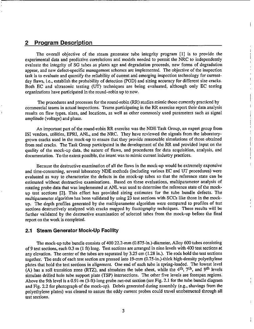
The mock-up tube bundle consists of 400 22.2-mm (0.875-in.)-diameter, Alloy 600 tubes consisting of 9 test sections, each 0.3 m (1 ft) long. Test sections are arranged in nine levels with 400 test sections at any elevation. The center of the tubes are separated by 3.25 cm (1.28 in.). Tie rods hold the test sections together. The ends of each test section are pressed into 19-mm (0.75-in.)-thick high-density polyethylene plates that hold the test sections in alignment. One end of each tube is spring-loaded. The lowest level (A) has a roll transition zone (RTZ), and simulates the tube sheet, while the 4 th, 7 th, and 9 th levels simulate drilled hole tube support plate (TSP) intersections. The other five levels are freespan regions. Above the 9th level is a 0.91-m (3-ft)-long probe run-out section (see Fig. 2.1 for the tube bundle diagram and Fig. 2.2 for photograph of the mock-up). Debris generated during assembly (e.g., shavings from the polyethylene plates) was cleared to assure the eddy current probes could travel unobstructed through all test sections.

3

V

Carbon steel tubes, O INAIII 120-l ~ Mehnialong, 19 68-mm slip fit (0 775-in.)-ID for Alloy 600

tubes

Polyethylene plate

Alloy 600,22 2-mm F (718-in )-diameter Tube support plates: tube sections (3600) Carbon steel are 305-mm(1 2-in) E 22 2-mm (3/4-In)-long thick (Drwng SGT11)

D

Divider plates (9): 1 B Polyethylene B 22 2-mm (3/4-in )thick (Drwng SGT13) A

[Spacer plate* Aluminum 6•3-mm (1/4-in)-thick (Drwng SGT1 8)

Simulated tube sheet 152-mm Tube bundle base plate: Carbon steel (6-in.)- 12.7-mm(1/2-in )-thick(Drwng SGT15) carbon-steel- ___ collar, over p 1 Alloy 600 tube] Eddy current Tube bundle support plate: Carbon steel

probe 25.4-mm (1-in )-thick

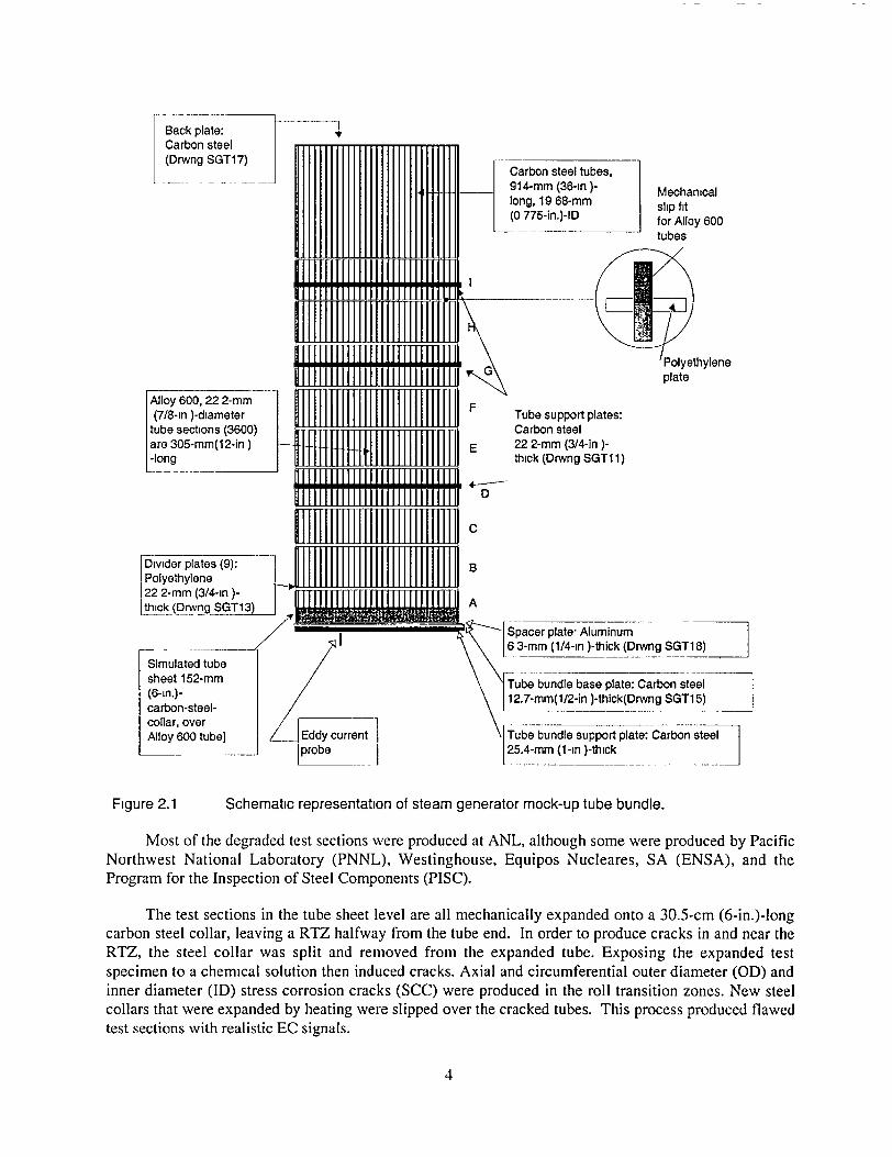
Figure 2.1 Schematic representation of steam generator mock-up tube bundle.

Most of the degraded test sections were produced at ANL, although some were produced by Pacific Northwest National Laboratory (PNNL), Westinghouse, Equipos Nucleares, SA (ENSA), and the Program for the Inspection of Steel Components (PISC).

The test sections in the tube sheet level are all mechanically expanded onto a 30.5-cm (6-in.)-long carbon steel collar, leaving a RTZ halfway from the tube end. In order to produce cracks in and near the RTZ, the steel collar was split and removed from the expanded tube. Exposing the expanded test specimen to a chemical solution then induced cracks. Axial and circumferential outer diameter (OD) and inner diameter (ID) stress corrosion cracks (SCC) were produced in the roll transition zones. New steel collars that were expanded by heating were slipped over the cracked tubes. This process produced flawed test sections with realistic EC signals.

4

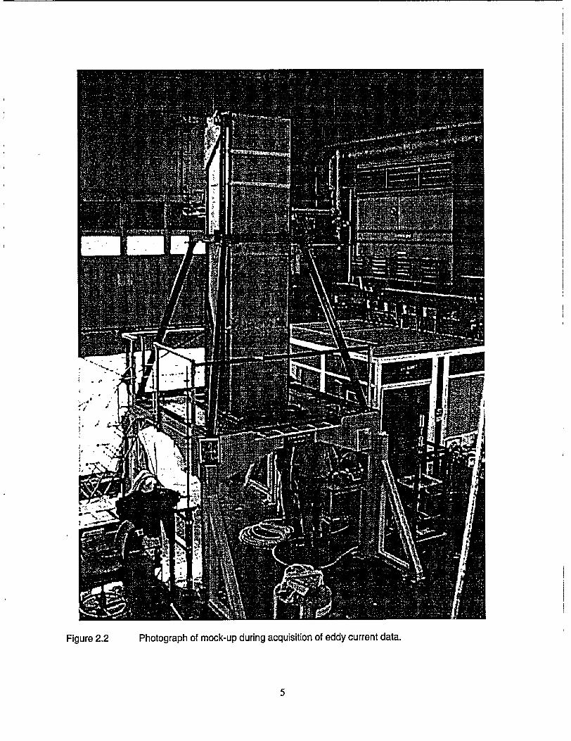
Figure 2.2 Photograph of mock-up during acquisition of eddy current data.

5

In the tube support plate TSP regions, filling the crevice with magnetic tape or a ferromagnetic fluid simulated magnetite in the crevices. A mixture of magnetite and copper bonded with epoxy simulated sludge deposits. Sludge was placed above the RTZ and at TSP intersections in some cases (see Figure 2.3 for photograph of sludge on a tube sheet test section). Many test sections had sludge or magnetite but no flaws. LODSCC and LIDSCC, both planar and segmented, and cracks with varying morphologies are present at TSP locations with and without denting (see Figure 2.4 for a photograph of a dent). Some flaw free test sections were dented. Cracks in the remaining five freespan levels are primarily LODSCC, both planar and segmented. Axial and circumferential cracks of ID and OD origin are found in the RTZ. A small number of other flaw types such as IGA and wear are placed in the tube bundle. The mock-up also contains test sections with electric-discharge-machined (EDM) notches and laser-cut slots. Table 2.1 summarizes the degradation types and their locations in the mock-up.

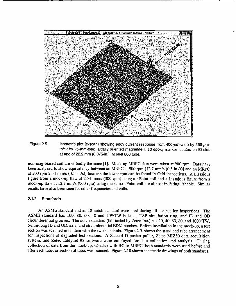
Magnetite-filled epoxy markers were placed at the ends of all test sections to provide a reference for the angular location of flaws when collecting data with a rotating or array probe. Figure 2.5 shows an isometric plot (c-scan) indicating the EC response from a 400-rim (0.016-in.)-wide by 250-jim (0.010-in.)-thick by 25-mm (1-in.)-long, axially oriented magnetite-filled epoxy marker located on the ID side, at the end of a test section. The data were acquired at 400 kHz with a 0.080-in. high-frequency shielded pancake coil. This test section also contains an outer-diameter stress corrosion crack (ODSCC) at the TSP intersection region. The analysts were instructed to ignore the region 1 in. from each test section end when carrying out their analysis.

Prior to assembly, flawed test sections in the tube bundle were examined with both bobbin coil (BC) and a three-coil rotating probe that incorporates a +Point coil, a 2.9-mm (0.115-in.) pancake coil, and a 2-mm (0.080-in.) shielded pancake coil. In addition to a full EC examination, many cracked test sections were examined by the dye-penetrant method before being incorporated into the mock-up tube bundle. If EC data, dye penetrant results or crack growth parameters indicated that a crack must be present, the test section was included in the mock-up. Because primary interest is with deep flaws, the majority of cracks selected for the mock-up had a +Point phase angle consistent with deep (>60% TW) cracks. Note that since the importance of obtaining POD data from deep flaws is greater than that for shallow ones, as expected, high voltage signals are more common in the mock-up than in operating steam generators. This is the result of the need for a large number of flaws when establishing a high POD (deep cracks) compared to the smaller number of flaws needed for a low POD (shallow cracks).

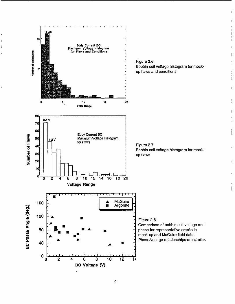
BC data from the mock-up were analyzed to show the distribution of voltages. The histograms (Figures 2.6 and 2.7 ) show a reasonable distribution of BC voltages (up to 20 V) for cracks and conditions, and cracks alone. Figure 2.6 shows the distribution for all signals called in the mock-up (cracks, dents, dings, wastage, and all overcall signals associated with artifacts). Figure 2.7 shows the distribution without the signals from artifacts or geometry. There are some cracks and conditions with voltages greater than 20 that are not shown in the histogram. Voltage and phase for mock-up cracks are similar in nature to field data such as from McGuire (Duke Power). Figure 2.8 shows a comparison of representative data from mock-up flaws and McGuire field data. The general scattering in the voltagephase representation is similar. Although the McGuire tubes are 19-mm (0.75-in.) rather than the mockup 22.2-mm (0.875-in.), they can be compared because the voltages from notches of the same %TW are set the same.

There are differences between the mock-up and an operating steam generator. The mock-up has short sections, not continuous tubes, and there are clear EC signals at the test section ends, which look like a throughwall 3600 circumferential notch or crack. The short lengths were necessary to allow realistic flaws to be made and to allow the mock-up to be reconfigured. There are no U-bends in the

6

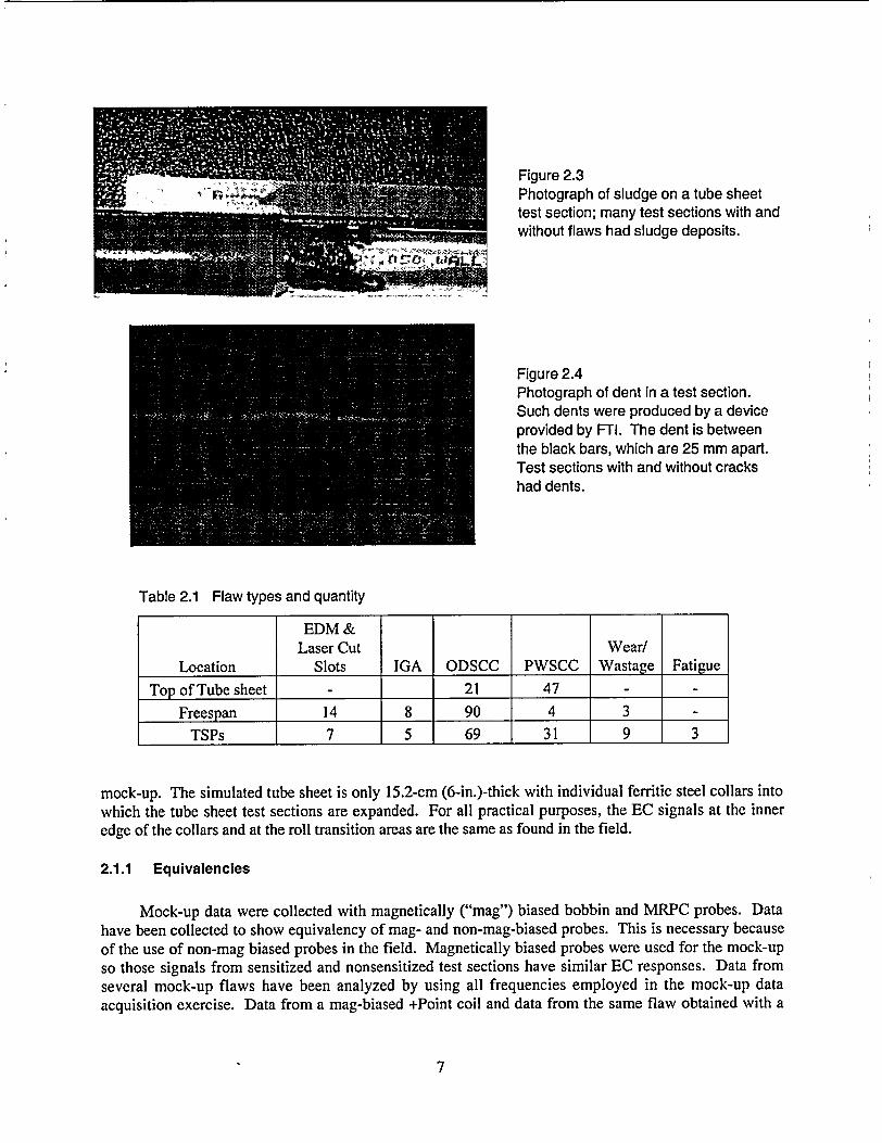
Figure 2.3 Photograph of sludge on a tube sheet test section; many test sections with and without flaws had sludge deposits.

Figure 2.4 Photograph of dent in a test section. Such dents were produced by a device provided by FTI. The dent is between the black bars, which are 25 mm apart. Test sections with and without cracks had dents.

Table 2.1 Flaw types and quantity

EDM & Laser Cut Wear/

Location Slots IGA ODSCC PWSCC Wastage Fatigue

Top of Tube sheet - 21 47 -

Freespan 14 8 90 4 3

TSPs 7 5 69 31 9 3

mock-up. The simulated tube sheet is only 15.2-cm (6-in.)-thick with individual ferritic steel collars into which the tube sheet test sections are expanded. For all practical purposes, the EC signals at the inner edge of the collars and at the roll transition areas are the same as found in the field.

2.1.1 Equivalencies

Mock-up data were collected with magnetically ("mag") biased bobbin and MRPC probes. Data have been collected to show equivalency of mag- and non-mag-biased probes. This is necessary because of the use of non-mag biased probes in the field. Magnetically biased probes were used for the mock-up so those signals from sensitized and nonsensitized test sections have similar EC responses. Data from several mock-up flaws have been analyzed by using all frequencies employed in the mock-up data acquisition exercise. Data from a mag-biased +Point coil and data from the same flaw obtained with a

7

,N.

Figure 2.5 Isometric plot (c-scan) showing eddy current response from 400-pm-wide by 250-,m

thick by 25-mm-long, axially oriented magnetite filled epoxy marker located on ID side at end of 22.2 mm (0.875-in.) Inconel 600 tube.

non-mag-biased coil are virtually the same [1]. Mock-up MRPC data were taken at 900 rpm. Data have been analyzed to show equivalency between an MRPC at 900 rpm [12.7 mm/s (0.5 in.Is)] and an MRPC at 300 rpm 2.54 mm/s (0.1 in./s)] because the lower rpm can be found in field inspections. A Lissajous figure from a mock-up flaw at 2.54 mm/s (300 rpm) using a +Point coil and a Lissajous figure from a mock-up flaw at 12.7 mm/s (900 rpm) using the same +Point coil are almost indistinguishable. Similar results have also been seen for other frequencies and coils.

2.1.2 Standards

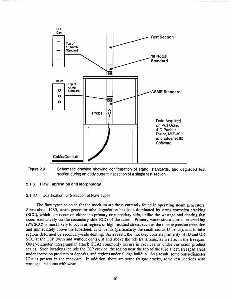
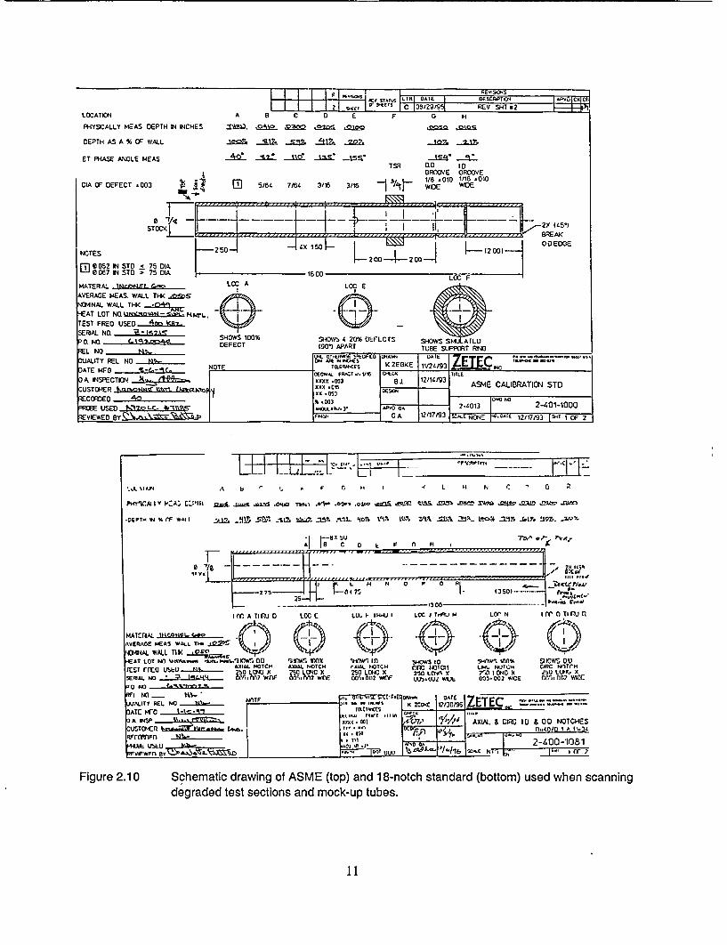
An ASME standard and an 18-notch standard were used during all test section inspections. The ASME standard has 100, 80, 60, 40 and 20%TW holes, a TSP simulation ring, and ID and OD circumferential grooves. The notch standard (fabricated by Zetec Inc.) has 20, 40, 60, 80, and 100%TW, 6-mm-long ID and OD, axial and circumferential EDM notches. Before installation in the mock-up, a test section was scanned in tandem with the two standards. Figure 2.9. shows the stand and tube arrangement for inspections of degraded test sections. A Zetec 4-D pusher-puller, Zetec MIZ30 data acquisition system, and Zetec Eddynet 98 software were employed for data collection and analysis. During collection of data from the mock-up, whether with BC or MRPC, both standards were used before and after each tube, or section of tube, was scanned. Figure 2.10 shows schematic drawings of both standards.

8

10 15

Volts Range

6 8 10 12 14 16 18 Voltage Range

Figure 2.6 Bobbin coil voltage histogram for mockup flaws and conditions

20

Figure 2.7 Bobbin coil voltage histogram for mockup flaws

20

0 2 4 6 8 BC Voltage (V)

10 12 11

Figure 2.8 Comparison of bobbin coil voltage and phase for representative cracks in mock-up and McGuire field data. Phase/voltage relationships are similar.

9

100

IS

580 z

0

80

7

6

5

4

3

2

S

LL

E z

0-1 V 0

0 Eddy Current BC

0 1-2 V Maximum Voltage Histogram for Flaws

0

0

0

0

A I I ---.-

1

0 2 4

160

120

80

40

'A

02

a)

0

OIL

0. t0 ccl

.,* I I I , ',,,I , * , £, i j i I '

IA McGuire " n Argonne

A

A A A

. , 3 I. ,, I 3 , I , , ,* I t ,I , i I , , ,0

OD Circ

Top of 18 Notch Standard

Holes

Cable/Conduit

Test Section

18 Notch Standard

,ASME Standard

Data Acquired on Pull Using 4-D Pusher Puller, MIZ-30 and Eddynet 95 Software

Figure 2.9 Schematic drawing showing configuration of stand, standards, and degraded test section during an eddy current inspection of a single test section

2.1.3 Flaw Fabrication and Morphology

2.1.3.1 Justification for Selection of Flaw Types

The flaw types selected for the mock-up are those currently found in operating steam generators. Since about 1980, steam generator tube degradation has been dominated by stress corrosion cracking (SCC), which can occur on either the primary or secondary side, unlike the wastage and denting that occur exclusively on the secondary side (OD) of the tubes. Primary water stress corrosion cracking (PWSCC) is most likely to occur at regions of high residual stress, such as the tube expansion transition and immediately above the tubesheet, at U-bends (particularly the small-radius U-bends), and in tube regions deformed by secondary-side denting. As a result, the mock-up consists primarily of ID and OD SCC at the TSP (with and without dents), at and above the roll transitions, as well as in the freespan. Outer-diameter intergranular attack (IGA) commonly occurs in crevices or under corrosion product scales. Such locations include the TSP crevice, the region near the top of the tube sheet, freespan areas under corrosion products or deposits, and regions under sludge buildup. As a result, some outer-diameter IGA is present in the mock-up. In addition, there are some fatigue cracks, some test sections with wastage, and some with wear.

10

LOCATION

PHYSICALLY MEAS DEPTH IN INCHES

DEPTH AS A % OF WALL

ET PHASE ANGLE MEAS

A B

TW?4

CIA OF DEFECT .003

I I Iz I _ 1 , 141, 1C 10512,J/O51C D E F 0 H

1417.A7. 2.Z

TSR QLD 1.0 GROO0VE GOO~VE

7/64 3/16 3/115 ~~ WIDE 1/16DE

t�V �III *I

NOTES F- 'Lu-4 I-?OO-ý- I-21.- - 0 002IN STD 75 CIA.

1, 067 IN STD 75 DIA 1600 OF MATERIAL IMM~lA- LEC A OE AVERAGE MEAS. WALL THI( ý= OMINAI. WALL TN1( -Q4~~ 1.-** HAT LOT NOAIa.M .MY-L

TEST FRED USED VAý31z.

SERL. Not SHW 100 SHYt 4 20% MIFLC 17 SHOWS SI ATILD 8E NDO DEFECT (90*1 APART TUBE SUFPPORT RING

OAIYRLNO M. Ar OAN "T DATE NFG S-e--le. NOTE YC0EN*105 K ZEGKE 11/24/3 ET CP OENA FPACT4.-.I/ CH*CK IL

0OA. INSPECTION AI~f= XXXX . 003 81 12/14/93 "ILE AIRAIN T

CUST3~4R K o?4t~ ~t~tXXI .055

-ROSE USDW7 0 2-4013 2-401-1000 REIWD yý = _G'AP0A, 12/17191 1 N0GJ E 12117193 SF- 1 OF 2

W±±jV:� �z V1�F.,kI JN A F r H I L I N

.DEPTH IN % F WE I -IV~i ~~ . JonI 'ot '176 ' %It -=- -U~k_ L.O*I a197w ._.. TIQZ_ .2//T.

I-BX tu B C 0 : F fl3 MH

IME A TINU 0

MATMrAL AVEPAGE MEAS WALL THI, j~;,

1,10W44AL WALL TIIK -09 ' 4AT LOT NO )IAY-K*, Acf..P5.IOWSOD0

rLST FRED Vll AXIAL. NOTCH -- L" 250 LONO X

0o NO f-,mn

Ri NO.... NA-.

)ATE MrCC ~ 2.

AXIAL. NOTCH 250 LONGX oon.M Monw

71,0 *,- YVA Ir

-- -- - ILAE N 0 P a R1

1300- c,.

LU. I- NK)I LOC J TrAJM LW N irC TIM1Jr

AIAL NOTCH CIM 140TC1 LIn.L NUTLI4 C'PC NnTCýH -250 LCON X 2-30 LII/M Y 7250 I ONO IX "~ L'~, , 300,1102 MOP U~-Ub.U1 WILJ 00 . 002 WOE 005n,002 WIDE

AXIAL & CIRG IU & GD NOTCHES

2-400-~O108 :.c N" Z -7 -

Figure 2.10 Schematic drawing of ASME (top) and 18-notch standard (bottom) used when scanning degraded test sections and mock-up tubes.

11

I

ly [D 5/64

AEVISKNS

lry"I'M

..........

REV SHT .2

2.1.3.2 Process for Fabricating Cracks

Alloy 600 test sections at ANL were cracked by using a IM aqueous solution of sodium tetrathionate at room temperature and atmospheric pressure, Techniques of localized environmental exposure, low applied load, and electrochemical potential were utilized to produce various crack geometries. Masking by coating areas of the tubes with lacquer was used to limit or localize the cracking area. The tubes were internally pressurized to generate hoop stresses to produce axial cracks and axially loaded to produce circumferential cracks. The times to produce cracking ranged from 20-1000 h, depending on the type of crack being produced. A variety of OD and ID crack geometries were produced; axial, circumferential, skewed, or combinations of these. Many of the specimens contained multiple cracks separated by short axial or circumferential ligaments. Prior to exposure to the sodium tetrathionate solution, specimens were sensitized by heat-treating at 600°C (11 12'F) for 48 h to produce a microstructure that is susceptible to cracking. Protective sleeves were used to prevent scratching or other mechanical damage to the test sections. An identification alphanumeric (ID) was permanently inscribed on the OD at both ends of each test section (Figure 2.11). All documentation is referenced to the test section ID. The mock-up was seeded with sensitized flaw-free test sections with and without artifacts so that the possibility of distinguishing sensitized from unsensitized test sections would not be an indicator that a flaw was present in that test section. In addition, many cracks were grown without sensitizing the test sections from Westinghouse.

Dye penetrant examinations were carried out for degradation on the OD. After completion of the degradation process, test sections were ultrasonically cleaned in high-purity water and dried. Dye penetrant examinations (PT) were performed in the vicinity of degradation for many test sections. The PT was carried out with Magnaflux Spotcheck SKL-SP Penetrant and SKC-S Cleaner/Remover. If SKL-SP Penetrant provided an unsatisfactory result, Zyglo 2L-27A Penetrant was used with Magnaflux Zyglo 2P-9f Developer as an alternate process.

The results of dye penetrant examination were documented by photography at 0.5-5X magnification. The photograph includes a calibrated scale so that magnification factor may be measured directly from the photograph (Figure 2.12).

Cross-sectional microscopy was performed on metallographically polished surfaces of many samples to provide documentation of the mock-up crack morphology. Figure 2.13 shows examples of LODSCC. The specimens were sometimes etched to delineate grain boundaries and other microstructural features, by electrolytic etching in 5% nitric acid-alcohol solution at 0.1 mA/mm2 for 5-30 seconds. The etching may also enhance contrast of the image, but the tip of a tight intergranular crack could be confused with a grain boundary. Photographic images were recorded at 10-500x magnifications. Cracks in the mock-up provided by PNNL (about 50) were produced by Westinghouse with a doped steam method that is proprietary and will not be discussed here. Axial and circumferential cracks both ID and OD were produced for the freespan, TSP, and roll transitions. Several IGA specimens, as well as fatigue and wastage samples, were also provided by PNNL. Figure 2.14 shows sketches of some dye penetrant images of ODSCC provided by PNNL for the mock-up.

2.1.3.3 Matrix of Flaws

Table 2.2 shows the distribution of flaw types. In this section, the flaw types and their depths are presented. The flaw depths are distributed into three ranges, 0-40%TW, 41%-80%TW, and 81-100%TW. The distribution is skewed toward deeper cracks. This is necessary to obtain high confidence in the high

12

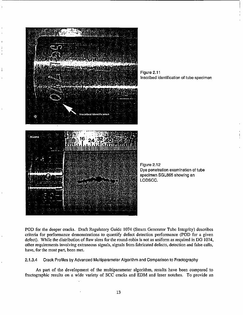
Figure 2.11 Inscribed identification of tube specimen

Figure 2.12 Dye penetration examination of tube specimen SGL865 showing an LODSCC.

POD for the deeper cracks. Draft Regulatory Guide 1074 (Steam Generator Tube Integrity) describes criteria for performance demonstrations to quantify defect detection performance (POD for a given defect). While the distribution of flaw sizes for the round-robin is not as uniform as required in DG 1074, other requirements involving extraneous signals, signals from fabricated defects, detection and false calls, have, for the most part, been met.

2.1.3.4 Crack Profiles by Advanced Multiparameter Algorithm and Comparison to Fractography

As part of the development of the multiparameter algorithm, results have been compared to fractographic results on a wide variety of SCC cracks and EDM and laser notches. To provide an

13

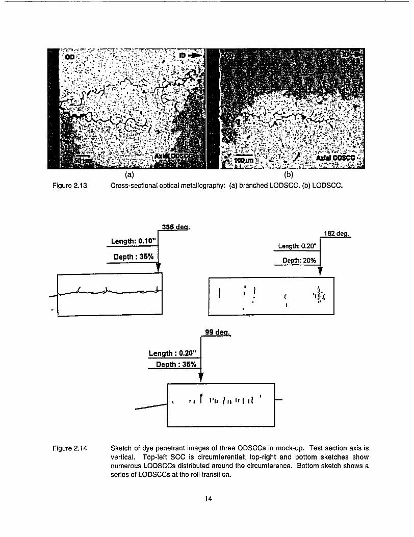
(a) (b) Figure 2.13 Cross-sectional optical metallography: (a) branched LODSCC, (b) LODSCC.

Length: 0.10"

Depth : 35%

335 de .182 deg

Length: 0.20"

Depth: 20%

Length : 0.20"

Depth : 35%

99 deg.

r

Sketch of dye penetrant images of three ODSCCs in mock-up. Test section axis is vertical. Top-left SCC is circumferential; top-right and bottom sketches show numerous LODSCCs distributed around the circumference. Bottom sketch shows a series of LODSCCs at the roll transition.

14

Figure 2.14

let

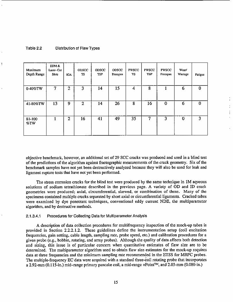
Table 2.2 Distribution of Flaw Types

objective benchmark, however, an additional set of 29 SCC cracks was produced and used in a blind test of the predictions of the algorithm against fractographic measurements of the crack geometry. Six of the benchmark samples have not yet been destructively analyzed because they will also be used for leak and ligament rupture tests that have not yet been performed.

The stress corrosion cracks for the blind test were produced by the same technique in IM aqueous solutions of sodium tetrathionate described in the previous page. A variety of OD and ID crack geometries were produced; axial, circumferential, skewed, or combination of these. Many of the specimens contained multiple cracks separated by short axial or circumferential ligaments. Cracked tubes were examined by dye penetrant techniques, conventional eddy current NDE, the multiparameter algorithm, and by destructive methods.

2.1.3.4.1 Procedures for Collecting Data for Multiparameter Analysis

A description of data collection procedures for multifrequency inspection of the mock-up tubes is provided in Section 2.2.2.1.2. These guidelines define the instrumentation setup (coil excitation frequencies, gain setting, cable length, sampling rate, probe speed, etc.) and calibration procedures for a given probe (e.g., bobbin, rotating, and array probes). Although the quality of data affects both detection and sizing, this issue is of particular concern when quantitative estimates of flaw size are to be determined. The multiparameter algorithm used to obtain flaw size estimates for the mock-up requires data at three frequencies and the minimum sampling rate recommended in the ETSS for MRPC probes. The multiple-frequency EC data were acquired with a standard three-toil rotating probe that incorporates a 2.92-mm (0.115-in.) mid-range primary pancake coil, a mid-range +PointTM, and 2.03-mm (0.080-in.)

15

EDM & Maximum Laser- Cut ODSCC ODSCC ODSCC PWSCC PWSCC PWSCC Wear/

Depth Range Slots IGA TS TSP Freespan TS TSP Freespan Wastage Fatigue

0-40%TW 7 2 3 14 15 4 8 1 6 0

41-80%TW 13 9 2 14 26 8 16 0 6 0

81-100 1 2 16 41 49 35 7 3 0 3 %TW

high-frequency pancake coil. Initial amplitude profiles are obtained from the +Point coil at a single channel. The final estimated depth profiles are obtained by using multichannel information from the midrange primary pancake coil for multiparameter data analysis. A detailed description of the algorithm and the data quality issue is given in Ref. 2, which also describes the conversion of Eddynet formatted data to a standard format for off-line analysis.

2.1.3.4.2 Fractography Procedures

For the destructive examination, the samples were heat-tinted before fracture to permit differentiation of the SCC and fracture opening surfaces. The specimens were then chilled in liquid nitrogen and cracks were opened by fracture. The fracture surfaces were examined macroscopically and with optical and scanning electron microscopy. The fractography and NDE data were digitized to obtain tabular and graphical comparisons of the depths as a function of axial or circumferential position. Welldefined markers on the test sections provided a means to accurately overlap the profiles.

Individual pieces of the specimen resulting from fracture are clearly identified, marked with new IDs, and documented.

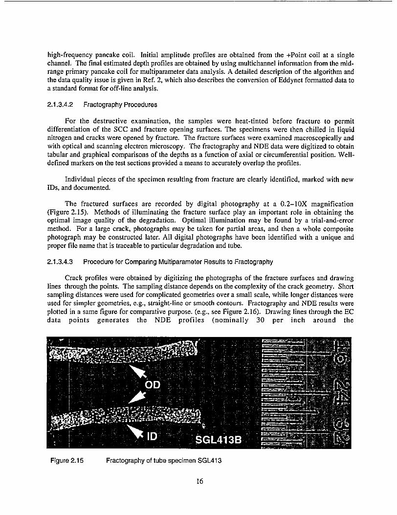
The fractured surfaces are recorded by digital photography at a 0.2-lOX magnification (Figure 2.15). Methods of illuminating the fracture surface play an important role in obtaining the optimal image quality of the degradation. Optimal illumination may be found by a trial-and-error method. For a large crack, photographs may be taken for partial areas, and then a whole composite photograph may be constructed later. All digital photographs have been identified with a unique and proper file name that is traceable to particular degradation and tube.

2.1.3.4.3 Procedure for Comparing Multiparameter Results to Fractography

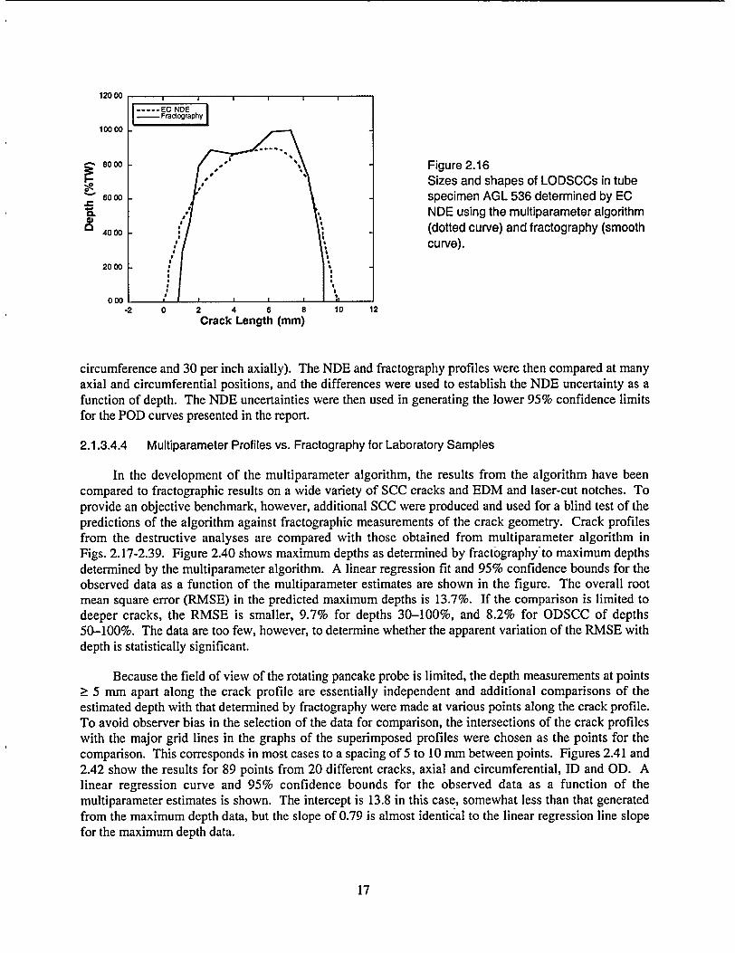
Crack profiles were obtained by digitizing the photographs of the fracture surfaces and drawing lines through the points. The sampling distance depends on the complexity of the crack geometry. Short sampling distances were used for complicated geometries over a small scale, while longer distances were used for simpler geometries, e.g., straight-line or smooth contours. Fractography and NDE results were plotted in a same figure for comparative purpose. (e.g., see Figure 2.16). Drawing lines through the EC data points generates the NDE profiles (nominally 30 per inch around the

Figure 2.15 Fractography of tube specimen SGL413

16

12000

10000

8000 o Figure 2.16 Sizes and shapes of LODSCCs in tube

800 "o" V0oo specimen AGL 536 determined by EC 400 NDE using the multiparameter algorithm

in 4000 (dotted curve) and fractography (smooth curve).

2000

000n,

.2 0 2 4 6 8 10 12

Crack Length (mm)

circumference and 30 per inch axially). The NDE and fractography profiles were then compared at many axial and circumferential positions, and the differences were used to establish the NDE uncertainty as a function of depth. The NDE uncertainties were then used in generating the lower 95% confidence limits for the POD curves presented in the report.

2.1.3.4.4 Multiparameter Profiles vs. Fractography for Laboratory Samples

In the development of the multiparameter algorithm, the results from the algorithm have been compared to fractographic results on a wide variety of SCC cracks and EDM and laser-cut notches. To provide an objective benchmark, however, additional SCC were produced and used for a blind test of the predictions of the algorithm against fractographic measurements of the crack geometry. Crack profiles from the destructive analyses are compared with those obtained from multiparameter algorithm in Figs. 2.17-2.39. Figure 2.40 shows maximum depths as determined by fractography to maximum depths determined by the multiparameter algorithm. A linear regression fit and 95% confidence bounds for the observed data as a function of the multiparameter estimates are shown in the figure. The overall root mean square error (RMSE) in the predicted maximum depths is 13.7%. If the comparison is limited to deeper cracks, the RMSE is smaller, 9.7% for depths 30-100%, and 8.2% for ODSCC of depths 50-100%. The data are too few, however, to determine whether the apparent variation of the RMSE with depth is statistically significant.

Because the field of view of the rotating pancake probe is limited, the depth measurements at points > 5 mm apart along the crack profile are essentially independent and additional comparisons of the estimated depth with that determined by fractography were made at various points along the crack profile. To avoid observer bias in the selection of the data for comparison, the intersections of the crack profiles with the major grid lines in the graphs of the superimposed profiles were chosen as the points for the comparison. This corresponds in most cases to a spacing of 5 to 10 mm between points. Figures 2.41 and 2.42 show the results for 89 points from 20 different cracks, axial and circumferential, ID and OD. A linear regression curve and 95% confidence bounds for the observed data as a function of the multiparameter estimates is shown. The intercept is 13.8 in this case, somewhat less than that generated from the maximum depth data, but the slope of 0.79 is almost identical to the linear regression line slope for the maximum depth data.

17

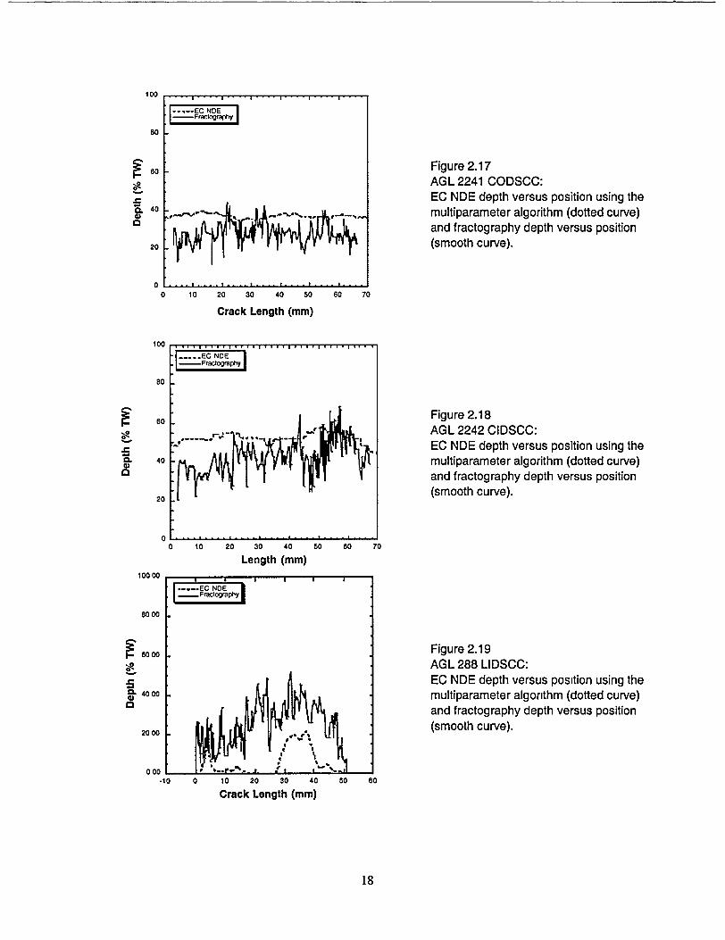
Figure 2.17 AGL 2241 CODSCC: EC NDE depth versus position using the multiparameter algorithm (dotted curve) and fractography depth versus position (smooth curve).

0 10 20 30 40 so 60 70

Crack Length (mm)

0 10 20 30 40 50

Length (mm)60 70

Figure 2.18 AGL 2242 CIDSCC: EC NDE depth versus position using the multiparameter algorithm (dotted curve) and fractography depth versus position (smooth curve).

Figure 2.19 AGL 288 LIDSCC: EC NDE depth versus position using the multiparameter algorithm (dotted curve) and fractography depth versus position (smooth curve).

Crack Length (mm)

18

100

80

C 40

20

0

. . . dogEC NOE S•o.__..__._hy100

80

60

40

20

0

CL

10000

8000

0.

CL 0

. . . . . . .. . .

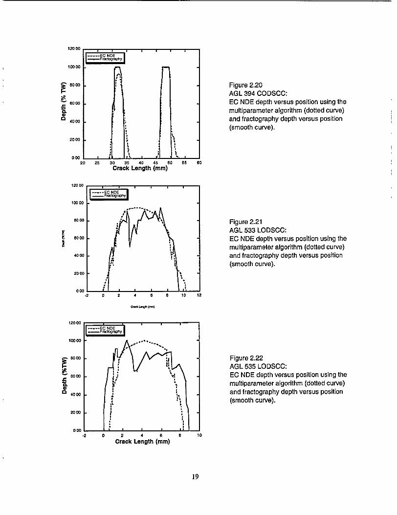
10000

"8000

6000

4000.

2000.

6OooL

20

12000

10000

8000

6000

4000

2000

000

12000

10000

S8000

00

4000

2000

000

C". L,.o Qa)

Figure 2.20 AGL 394 CODSCC: EC NDE depth versus position using the multiparameter algorithm (dotted curve) and fractography depth versus position (smooth curve).

Figure 2.21 AGL 533 LODSCC: EC NDE depth versus position using the multiparameter algorithm (dotted curve) and fractography depth versus position (smooth curve).

Figure 2.22 AGL 535 LODSCC: EC NDE depth versus position using the multiparameter algorithm (dotted curve) and fractography depth versus position (smooth curve).

-2 0 2 4 6 8 10

Crack Length (mm)

19

12000

25 30 35 40 45 60 65 60 Crack Length (mm)

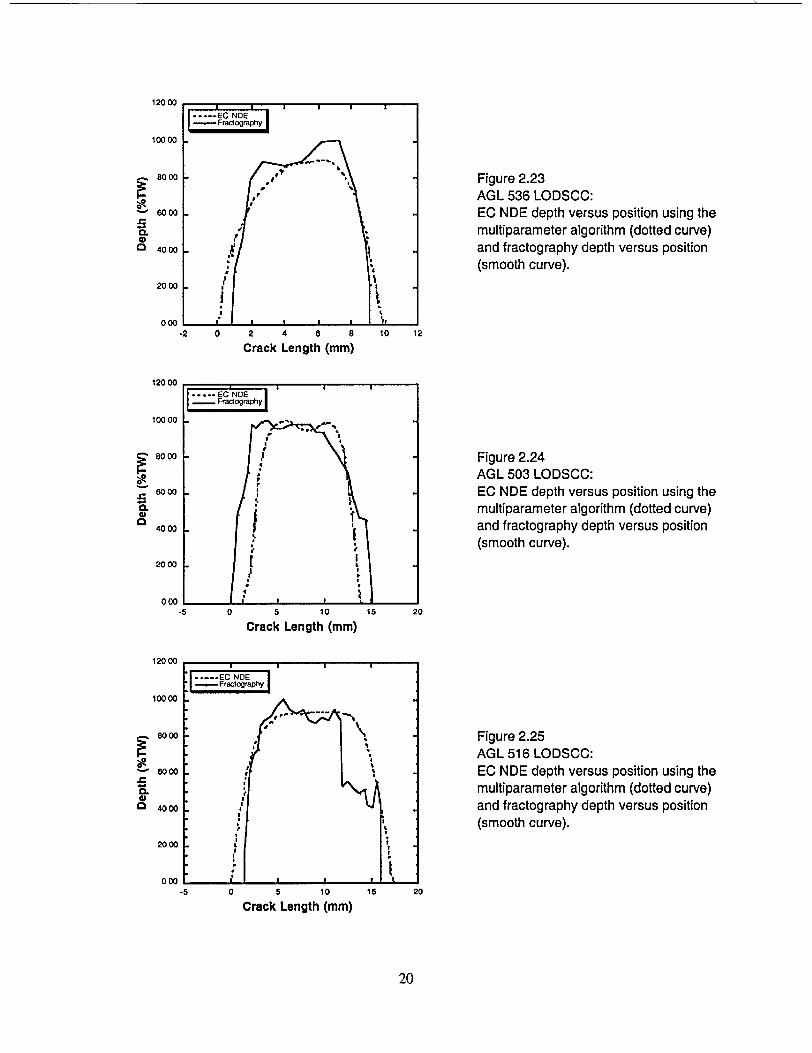
10000

8000

S6000

8) o 4000

20 0O

000

12000

10000

S8000

ORO ~6000 40.

20O

4000

12000

10000 12000

10000

4000

2000

000O

Crack Length (mm)

-5 0 5 10

Crack Length (mm)

Figure 2.23 AGL 536 LODSCC: EC NDE depth versus position using the multiparameter algorithm (dotted curve) and fractography depth versus position (smooth curve).

10 12

Figure 2.24 AGL 503 LODSCC: EC NDE depth versus position using the multiparameter algorithm (dotted curve) and fractography depth versus position (smooth curve).

Figure 2.25 AGL 516 LODSCO: EC NDE depth versus position using the multiparameter algorithm (dotted curve) and fractography depth versus position (smooth curve).

15 20

20

12000

-2 0 2 4 6 8

Crack Length (mm)

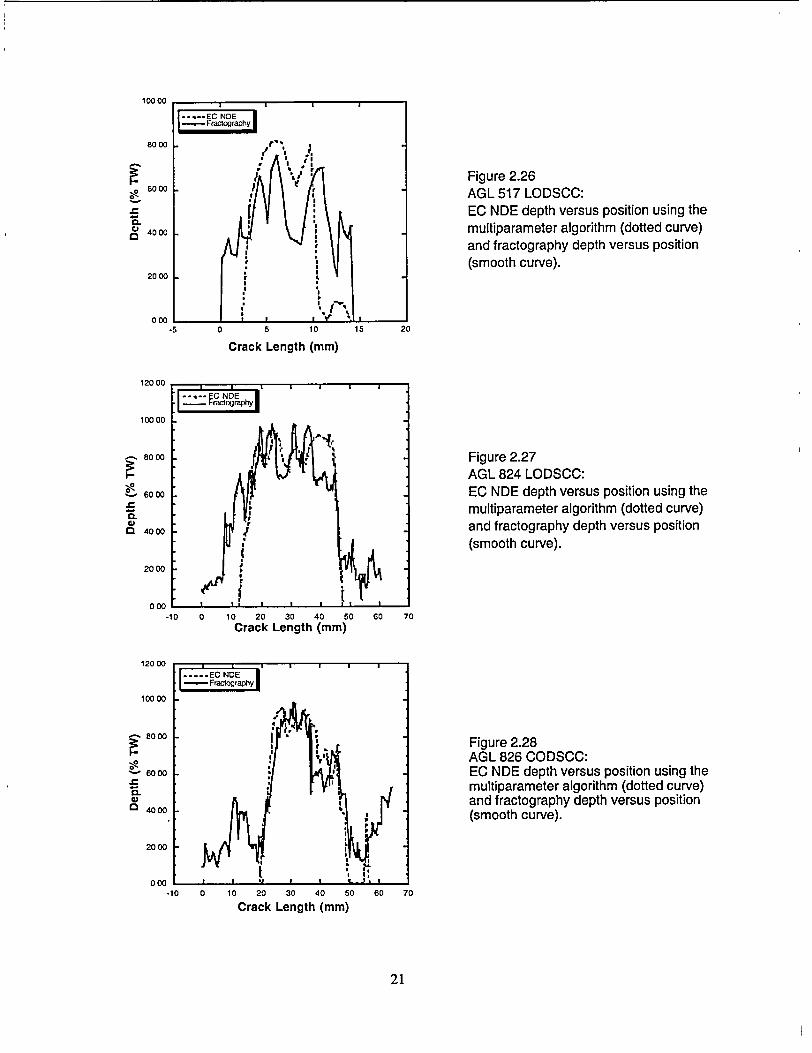
5 10

Crack Length (mm)

Figure 2.26 AGL 517 LODSCC: EC NDE depth versus position using the multiparameter algorithm (dotted curve) and fractography depth versus position (smooth curve).

15 20

10 0 10 20 30 40 50 60 Crack Length (mm)

000 L 1 1 - .

-10 0 10 20 30 40 50 60 70

Crack Length (mm)

Figure 2.27 AGL 824 LODSCO: EC NDE depth versus position using the multiparameter algorithm (dotted curve) and fractography depth versus position (smooth curve).

70

12000

10000

S8000

6000

Co 4000

2000

000

12000

10000

8000

6000

CI

o 4000

2000

21

10000

8000

6000

4000

2000

000.5

Er NDE l - Fractography"I --E D

)l .1

r

Figure 2.28 AGL 826 CODSCC: EC NDE depth versus position using the multiparameter algorithm (dotted curve) and fractography depth versus position (smooth curve).

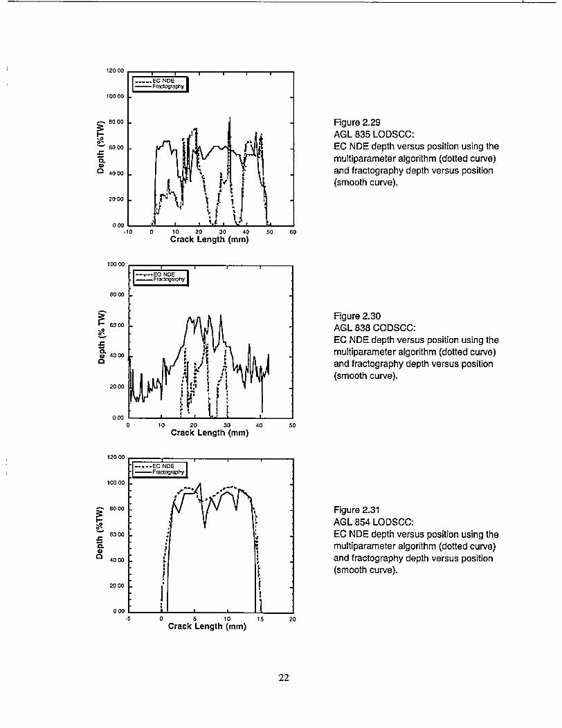
10000

S8000

6000 0..

2000

000

10000

8000

6000

w 4000

2000

0 000 10 20 30

Crack Length (mm)

Figure 2.29 AGL 835 LODSCC: EC NDE depth versus position using the multiparameter algorithm (dotted curve) and fractography depth versus position (smooth curve).

50 60

Figure 2.30 AGL 838 CODSCC: EC NDE depth versus position using the multiparameter algorithm (dotted curve) and fractography depth versus position (smooth curve).

40 50

5 10

Crack Length (mm)

Figure 2.31 AGL 854 LODSCC: EC NDE depth versus position using the multiparameter algorithm (dotted curve) and fractography depth versus position (smooth curve).

22

12000

10 0 10 20 30 40

Crack Length (mm)

12000

10000

8000

0 O0 60O00

4000

2000

000-5

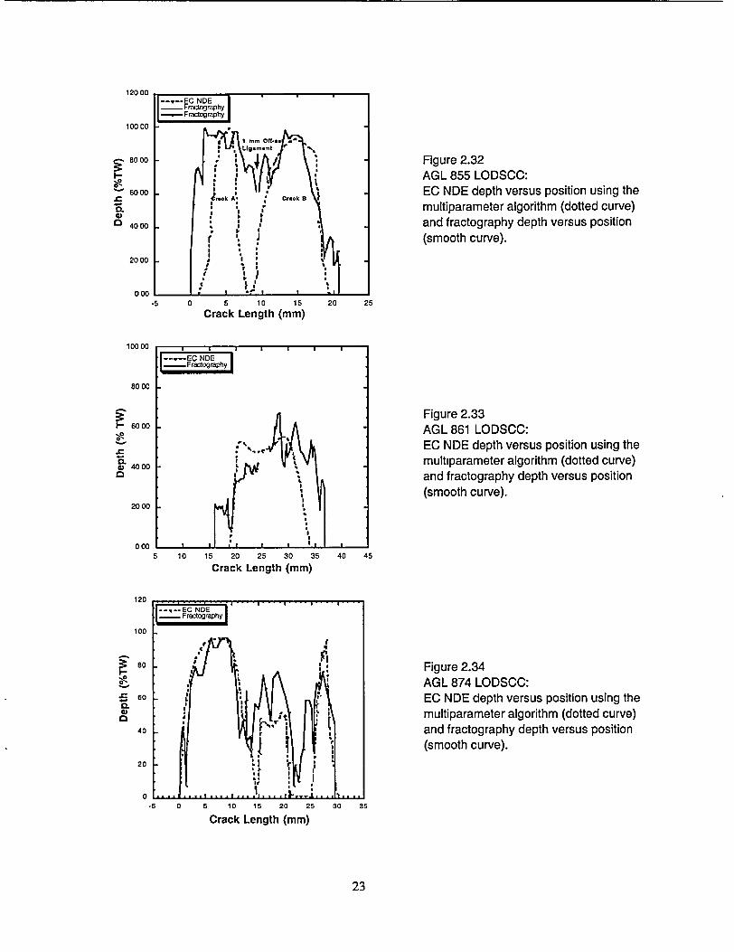
10000

8000

S6000

CL

- 4000

2000

000

10000

8000

~6000

C) 4000

2000

000

120

100

o80

a,.

CL 40

20

0

10 15 20 25 30 35 40 45

Crack Length (mm)

Figure 2.32 AGL 855 LODSCC: EC NDE depth versus position using the multiparameter algorithm (dotted curve) and fractography depth versus position (smooth curve).

20 25

Figure 2.33 AGL 861 LODSCC: EC NDE depth versus position using the multiparameter algorithm (dotted curve) and fractography depth versus position (smooth curve).

Figure 2.34 AGL 874 LODSCC: EC NDE depth versus position using the multiparameter algorithm (dotted curve) and fractography depth versus position (smooth curve).

-5 0 5 10 15 20 25 30 35

Crack Length (mm)

23

12000

.5 0 5 10 15

Crack Length (mm)

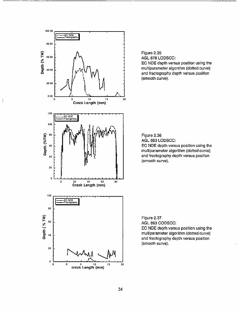
10000

8000

6000

4000

2000

000

120

100

Figure 2.35 AGL 876 LODSCC: EC NDE depth versus position using the multiparameter algorithm (dotted curve) and fractography depth versus position (smooth curve).

20

Figure 2.36 AGL 883 LODSOC: EC NDE depth versus position using the multiparameter algorithm (dotted curve) and fractography depth versus position (smooth curve).

0 20 40 60 80

Crack Length (mm)

Figure 2.37 AGL 893 CODSCC: EC NDE depth versus position using the multiparameter algorithm (dotted curve) and fractography depth versus position (smooth curve).

15 20

24

0-.

CL

5 10 15

Crack Length (mm)0

80 I.

60

CL 4o

40

20

0

.. . . . . . . . . . .. . I . . . . . . . . .

[ EC NOE -. Fractography

100

80

60

a 40

20

0-5 0 5 10

crack Length (mm)

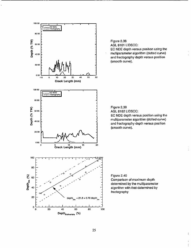
8000

6000

0.

4) 4000 2000

000

-10

10000 II 8000

I- 6000

-0

0. 4000 4)

2000

000 L

Figure 2.38 AGL 8161 LIDSCC: EC NDE depth versus position using the multiparameter algorithm (dotted curve) and fractography depth versus position (smooth curve).

Figure 2.39 AGL 8162 LIDSCC: EC NDE depth versus position using the multiparameter algorithm (dotted curve) and fractography depth versus position (smooth curve).

5 10 15 20 Crack Length (mm)

0 20 40 60

DeptlM.1tvard:e (%)

Figure 2.40 Comparison of maximum depth determined by the multiparameter algorithm with that determined by fractography

80 100

25

10000

0 10 20 30 40 50 60

Crack Length (mm)

100

80

60

0.°

w 40

20

20

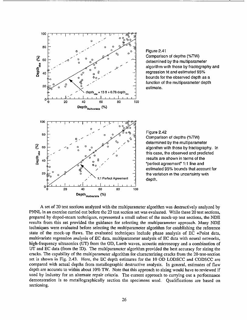
0 0- Figure 2.41 o ... " j 00

F. 60 .0 ý 1 o oo- Comparison of depths (%TW) 0 0- 0 determined by the multiparameter

0 10' algorithm with those by fractography and 40 - 0 0 8 regression fit and estimated 95% o0

-o 0 0 bounds for the observed depth as a 0 0 If . function of the multiparameter depth

estimate. 1 d 138+0.78 depth

0 20 40 60 80 100

DepthMultvarlat (%)

100 0 00

0 0 0

80 0 0 o Figure 2.42

-0 o Comparison of depths (%TW) 60 _ 0 /' determined by the multiparameter

0 0 0 S6 - -- o o0 0 / o / algorithm with those by fractography. In

0008 0 othis case, the observed and predicted / results are shown in terms of the

S o/ "perfect agreement" 1:1 line and estimated 95% bounds that account for

2o 0 o oI0 0 0 the variation in the uncertainty with / 1:1 Perfect Agreement depth.

0 20 40 60 80 100

Depth Mulvarlate (%)

A set of 20 test sections analyzed with the multiparameter algorithm was destructively analyzed by PNNL in an exercise carried out before the 23 test section set was evaluated. While these 20 test sections, prepared by doped-steam techniques, represented a small subset of the mock-up test sections, the NDE results from this set provided the guidance for selecting the multiparameter approach. Many NDE techniques were evaluated before selecting the multiparameter algorithm for establishing the reference state of the mock-up flaws. The evaluated techniques include phase analysis of EC +Point data, multivariate regression analysis of EC data, multiparameter analysis of EC data with neural networks, high-frequency ultrasonics (UT) from the OD, Lamb waves, acoustic microscopy and a combination of UT and EC data (from the ID). The multiparameter algorithm provided the best accuracy for sizing the cracks. The capability of the multiparameter algorithm for characterizing cracks from the 20-test-section set is shown in Fig. 2.43. Here, the EC depth estimates for the 10 OD LODSCC and CODSCC are compared with actual depths from metallographic destructive analysis. In general, estimates of flaw depth are accurate to within about 10% TW. Note that this approach to sizing would have to reviewed if used by industry for an alternate repair criteria. The current approach to carrying out a performance demonstration is to metallographically section the specimens used. Qualifications are based on sectioning.

26

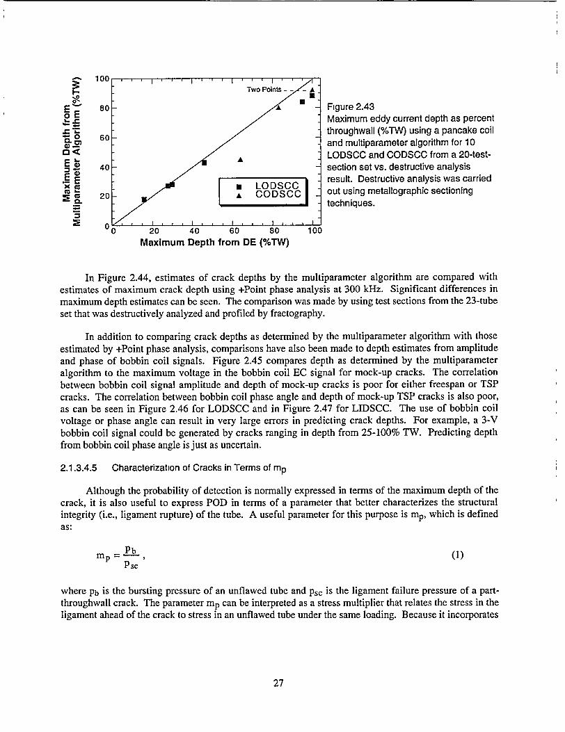
o• 100 1 1 1 .I I • Two Points -- - A

E 80 Figure 2.43 0• Maximum eddy current depth as percent

'-Z " throughwall (%TW) using a pancake coil 9.o) Q -and multiparameter algorithm for 10 SA LODSCC and CODSCC from a 20-testE 4 40 section set vs. destructive analysis

.E result. Destructive analysis was carried X( ca LODSCC.

cc 20 CODSCC out using metallographic sectioning - techniques.

.1,, I I , , ,I , , I

0 20 40 60 80 100

Maximum Depth from DE (%TW)

In Figure 2.44, estimates of crack depths by the multiparameter algorithm are compared with estimates of maximum crack depth using +Point phase analysis at 300 kHz. Significant differences in maximum depth estimates can be seen. The comparison was made by using test sections from the 23-tube set that was destructively analyzed and profiled by fractography.

In addition to comparing crack depths as determined by the multiparameter algorithm with those estimated by +Point phase analysis, comparisons have also been made to depth estimates from amplitude and phase of bobbin coil signals. Figure 2.45 compares depth as determined by the multiparameter algorithm to the maximum voltage in the bobbin coil EC signal for mock-up cracks. The correlation between bobbin coil signal amplitude and depth of mock-up cracks is poor for either freespan or TSP cracks. The correlation between bobbin coil phase angle and depth of mock-up TSP cracks is also poor, as can be seen in Figure 2.46 for LODSCC and in Figure 2.47 for LIDSCC. The use of bobbin coil voltage or phase angle can result in very large errors in predicting crack depths. For example, a 3-V bobbin coil signal could be generated by cracks ranging in depth from 25-100% TW. Predicting depth from bobbin coil phase angle is just as uncertain.

2.1.3.4.5 Characterization of Cracks in Terms of mp

Although the probability of detection is normally expressed in terms of the maximum depth of the crack, it is also useful to express POD in terms of a parameter that better characterizes the structural integrity (i.e., ligament rupture) of the tube. A useful parameter for this purpose is mp, which is defined as:

Pb(1 mp = m 1 Psc

where Pb is the bursting pressure of an unflawed tube and Psc is the ligament failure pressure of a partthroughwall crack. The parameter mp can be interpreted as a stress multiplier that relates the stress in the ligament ahead of the crack to stress in an unflawed tube under the same loading. Because it incorporates

27

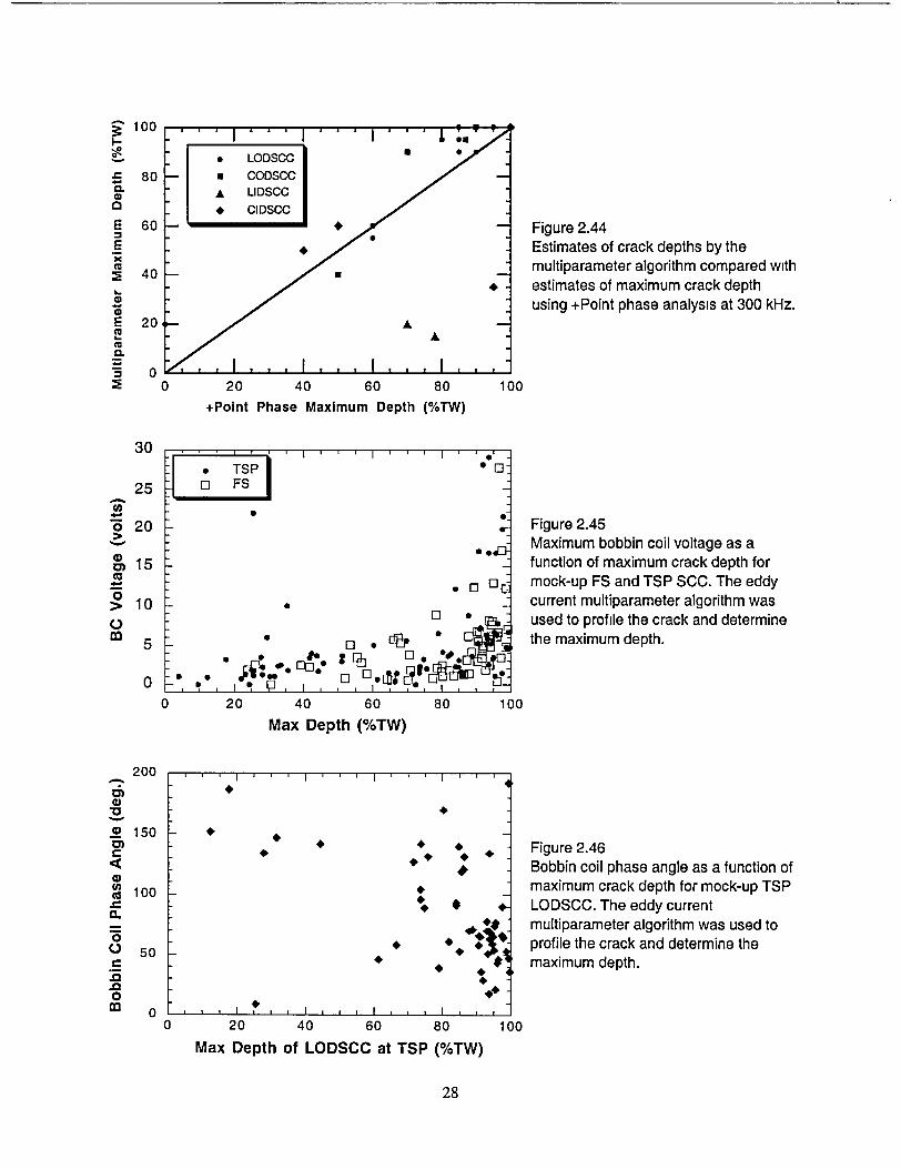
100 ' ' .

SLODSCC 0

. 80 I. cODSCCIA LIDSCC a • ClDSCC: 0

E 60 Figure 2.44 E Estimates of crack depths by the MX• multiparameter algorithm compared with S40

*4Oestimates of maximum crack depth using +Point phase analysis at 300 kHz.

E 20 A A

CL 0•' *, , , I , I , , I , , I , , ,

S0 S0 20 40 60 80 100

+Point Phase Maximum Depth (%TW)

3 0 . . . . . . .

* TSP '0 25 0 FS

"620 Figure 2.45 "Maximum bobbin coil voltage as a

S15 function of maximum crack depth for 0 D mock-up FS and TSP SCC. The eddy

> 10 - current multiparameter algorithm was ] . used to profile the crack and determine

*• " *-the maximum depth. r%. o . @*.F.~ . [ .% _. *

0I • . I , , I 0 20 40 60 80 100

Max Depth (%TW)

200

. 150 + 4 * Figure 2.46

* ;Bobbin coil phase angle as a function of 2 100 maximum crack depth for mock-up TSP

• 4 • LODSCC. The eddy current "•", * multiparameter algorithm was used to

o 5 ** profile the crack and determine the .= 50 maximum depth.

.0 o o , I •

0 20 40 60 80 100 Max Depth of LODSCC at TSP (%TW)

28

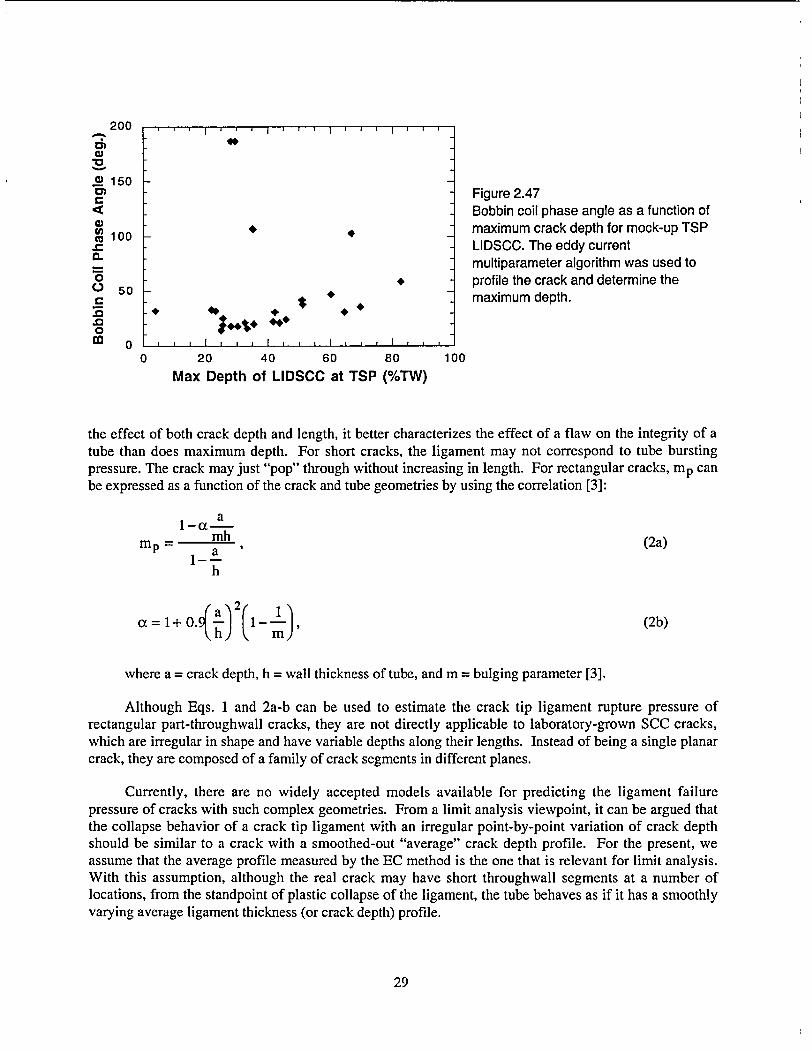
200

M*

_.2 150 150 Figure 2.47

Bobbin coil phase angle as a function of •10maximum crack depth for mock-up TSP u)100

LIDSCC. The eddy current multiparameter algorithm was used to

o profile the crack and determine the

maximum depth.

o

0 20 40 60 80 100

Max Depth of LIDSCC at TSP (%TW)

the effect of both crack depth and length, it better characterizes the effect of a flaw on the integrity of a tube than does maximum depth. For short cracks, the ligament may not correspond to tube bursting pressure. The crack may just "pop" through without increasing in length. For rectangular cracks, mp can be expressed as a function of the crack and tube geometries by using the correlation [3]:

a

mh (2a) mp- a )

h

a= 1+ 0 . 1-( , (2b)

where a = crack depth, h = wall thickness of tube, and m = bulging parameter [3].

Although Eqs. 1 and 2a-b can be used to estimate the crack tip ligament rupture pressure of rectangular part-throughwall cracks, they are not directly applicable to laboratory-grown SCC cracks, which are irregular in shape and have variable depths along their lengths. Instead of being a single planar crack, they are composed of a family of crack segments in different planes.

Currently, there are no widely accepted models available for predicting the ligament failure pressure of cracks with such complex geometries. From a limit analysis viewpoint, it can be argued that the collapse behavior of a crack tip ligament with an irregular point-by-point variation of crack depth should be similar to a crack with a smoothed-out "average" crack depth profile. For the present, we assume that the average profile measured by the EC method is the one that is relevant for limit analysis. With this assumption, although the real crack may have short throughwall segments at a number of locations, from the standpoint of plastic collapse of the ligament, the tube behaves as if it has a smoothly varying average ligament thickness (or crack depth) profile.

29

Because the measured crack depth profile by ANL's EC algorithm is generally not rectangular (e.g., see Fig. 2.48), the following procedure was used to establish the length and depth of an equivalent rectangular crack: [3]

(a) Choose a crack depth d. and assume that any crack segment with depth d < d, does not adversely affect the crack tip ligament rupture pressure of the tube (Fig. 2.48a). In other words, replace the original crack depth profile by a new crack depth profile in which any crack segment with depth d<do is replaced by d = 0 (Fig. 2.48b). The choice of do fixes the candidate equivalent rectangular crack length (Lo).

(b) The depth of the candidate equivalent rectangular crack is determined by equating its area to the area under the crack depth profile defined in step 1 (Fig. 2.48b). For example, in Figs. 2.48 a-b, the choice of d, = 50% fixes the length and depth of the candidate equivalent rectangular crack at 9 mm and 70%, respectively.

(c) Generate a series of candidate equivalent rectangular cracks by parametrically varying do and calculate the ligament rupture pressures for all the candidates (Fig 2.49).

(d) The equivalent rectangular crack corresponds to the lowest ligament rupture pressure (Figure 2.49).

This procedure has been automated by systematically choosing various candidate equivalent crack lengths Lo (instead of do), determining the corresponding candidate equivalent crack depths, and selecting the equivalent crack length, depth, and value of mp that correspond to the minimum ligament rupture pressure.

2.1.3.5 Summary of Sizing Accuracy

The RMSE values from the data of Figs. 2.17 to 2.39, for various binned depth ranges, are presented in Tables 2.3 and 2.4. In Table 2.3, the depth ranges are given in terms of the metallographic depths. This is useful when assessing the capability of the multiparameter algorithm for cracks of a certain depth. In Table 2.3. the depth ranges are given in terms of the predicted depths. This is more useful when assessing the uncertainty in predicted depths. In Figure 2.50, the standard deviation in depth (in %TW) is plotted against the maximum depth. The largest uncertainty is in the 50-70%TW range. While the deviation is small for the shallow cracks, it represents a relatively large error. For example, the standard deviation for 20%TW is 12%TW.

The overall RMSE for all cracks of all depths is 15.1%, but it is somewhat misleading to look at this overall value because there is a significant variation in the RMSE with depth. The RMSE value is significantly better for the 80-100%TW bin than for the other depth bins.

In Table 2.4, two sets of RMSE values are given; one is based on the values obtained directly from the multiparameter algorithm and the other on "corrected" values obtained from the regression fit shown in Fig. 2.41. For the shallowest cracks, the "corrected" values give a significantly lower RMSE value, but when all the data are considered, the differences in the RMSE for corrected and uncorrected predictions are small. This indicates that there is little systematic bias in the predictions of the multiparameter algorithm, i.e., the errors are random.

30

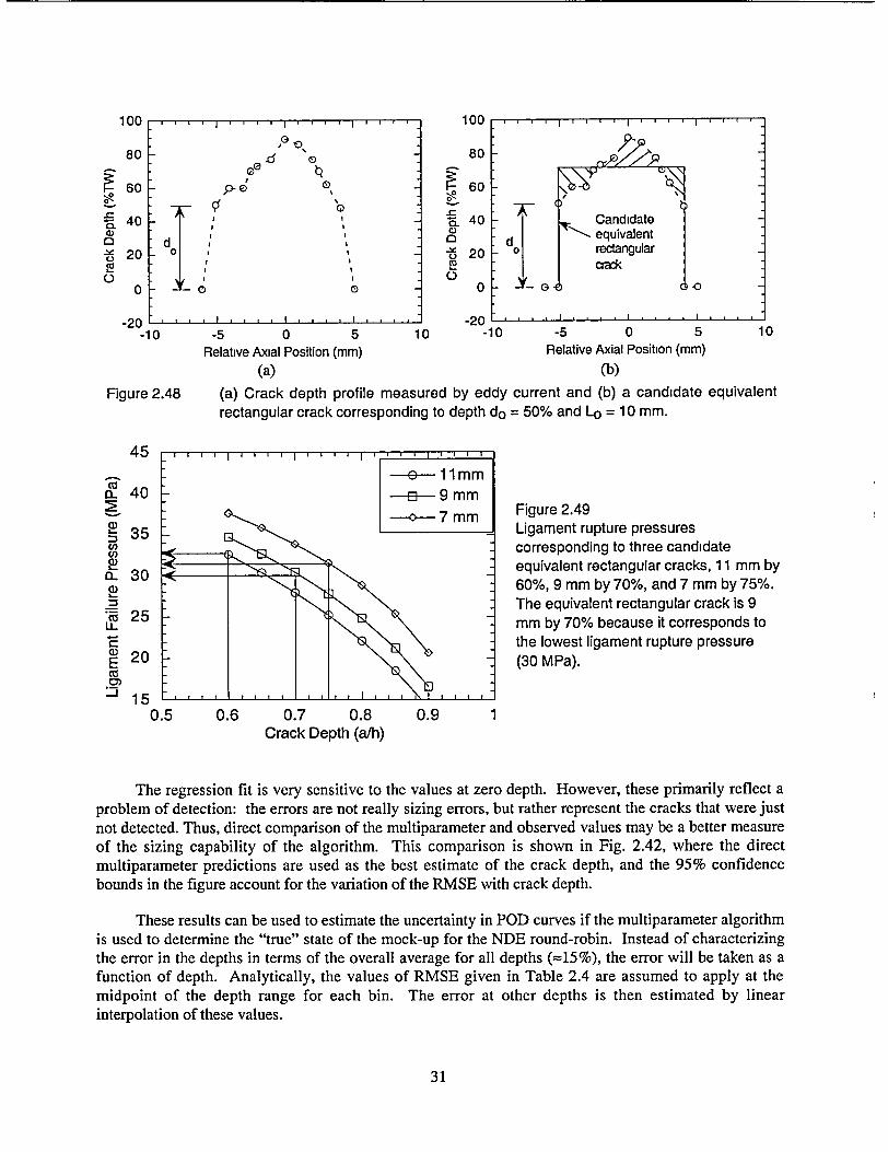
-5 0 5 Relative Axial Position (mm)

(a)

11

100

80

S60

.40 20

0

-20 0

Go

dn

d{, , I ;

0 0

-5 0 5 10

Relative Axial Position (mm)

(b)

(a) Crack depth profile measured by eddy current and (b) a candidate equivalent rectangular crack corresponding to depth do = 50% and Lo = 10 mm.

Ba- 9 MM o 7 mm Figure 2.49

Ligament rupture pressures corresponding to three candidate equivalent rectangular cracks, 11 mm by 60%, 9 mm by 70%, and 7 mm by 75%. The equivalent rectangular crack is 9 mm by 70% because it corresponds to the lowest ligament rupture pressure (30 MPa).

0.6 0.7 0.8 0.9 Crack Depth (a/h)

The regression fit is very sensitive to the values at zero depth. However, these primarily reflect a problem of detection: the errors are not really sizing errors, but rather represent the cracks that were just not detected. Thus, direct comparison of the multiparameter and observed values may be a better measure of the sizing capability of the algorithm. This comparison is shown in Fig. 2.42, where the direct multiparameter predictions are used as the best estimate of the crack depth, and the 95% confidence bounds in the figure account for the variation of the RMSE with crack depth.

These results can be used to estimate the uncertainty in POD curves if the multiparameter algorithm is used to determine the "true" state of the mock-up for the NDE round-robin. Instead of characterizing the error in the depths in terms of the overall average for all depths (=15%), the error will be taken as a function of depth. Analytically, the values of RMSE given in Table 2.4 are assumed to apply at the midpoint of the depth range for each bin. The error at other depths is then estimated by linear interpolation of these values.

31

100

80

S60

E 40

20 " 20

0

.-9n10

Candidate d •ý equivalent di

0rectangular crack

(2 -O

-10

Figure 2.48

45

n40

35

a. 30

2 S25

a 20

"15 L

0.5

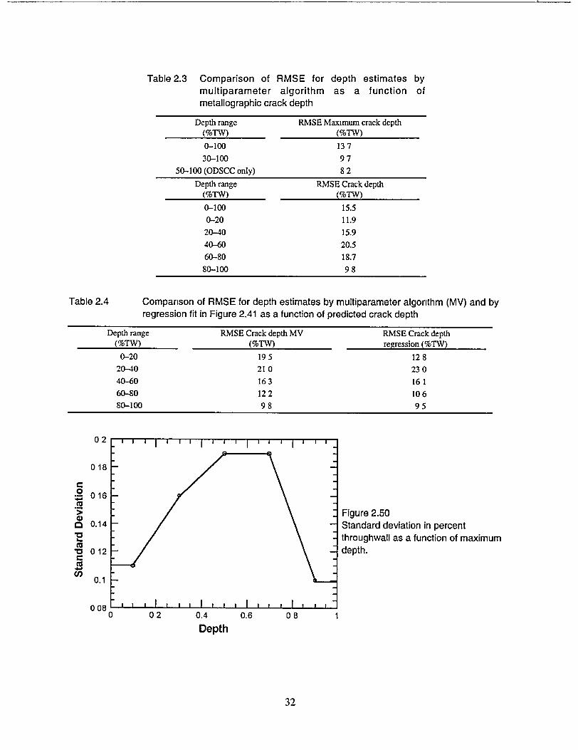
Table 2.3 Comparison of RMSE for depth estimates by multiparameter algorithm as a function of metallographic crack depth

Depth range (%TW)

0-100

30-100

50-100 (ODSCC only)

RMSE Maximum crack depth (%TW)

137

97

82

Depth range RMSE Crack depth (%TW) (%TW)

0-100 15.5 0-20 11.9

20-40 15.9

40-60 20.5 60-80 18.7

80-100 98

Comparison of RMSE for depth estimates by multiparameter algorithm (MV) and by regression fit in Figure 2.41 as a function of predicted crack depth

Depth range RMSE Crack depth MV RMSE Crack depth (%TW) (%TW) regression (%TW)

0-20 195 128 20-40 210 230

40-60 163 161 60-80 122 106 80-100 98 95

0 02 0.4

Depth

Figure 2.50 Standard deviation in percent throughwall as a function of maximum depth.

0.6 08 1

32

Table 2.4

02

018

0 . 016

o 0.14

"0 012

0.1

0 08

2.1.3.6 Reference State Table Summary for Mock-up

The reference state table for the mock-up provides all the relevant information for analyzing the round-robin analysts' results. Tables 2.5 and 2.6 highlight the primary information for a flaw in the table. The flaw type, BC volts, BC phase, whether ID or OD, three-letter code for the flaw, maximum depth as determined by multiparameter algorithm, flaw length, average depth, and mp are all included in the flaw table. Not shown are flaw location in the mock-up (row, column, and level) and beginning and end points of the flaw, in BC data points. The test sections included in the table data are those for which mp was determined. As a result, these tables present data from the flaws that have relatively large EC signals, permitting the profiling to be carried out accurately and leading to an accurate value of mp. Table 2.5 shows the values for TSP SCC, while Table 2.6 shows the values for freespan SCC.

2.2 Design and Organization of Round-Robin

A very important aspect of developing the round-robin (RR) exercise was input from an NDE Task Group. The Task Group helped define the parameters found in a field inspection and provided input on how to ensure that the RR mimicked an in-service (ISI) inspection. Members of the Task Group are from utilities, vendors, EPRI, NRC, and ANL. The industry members are G. Henry and J. Benson (EPRI), T. Richards and R. Miranda (FTI), D. Adamonis and R. Maurer (Westinghouse), D. Mayes (Duke), S. Redner (Northern States Power), and B. Vollmer and N. Farenbaugh (Zetec).

The Task Group provided input related to the make-up of the mock-up, the quality of the data collected for the RR, the nature of the flaws, procedures for analyzing data, and documentation. The Task Group helped meet the goal of providing an RR exercise that represents, as closely as possible, a true field inspection. The Task Group provided input on the analysis guidelines, data acquisition, degradation assessment, training manual, and examination technique specification sheets (ETSSs). The RR began only after the Task Group approved the documentation used for the RR and concluded that flaws in the mock-up had EC signals similar to signals observed under field conditions. In addition, opinions were expressed on how to handle spin calls, how to handle the logistics of distributing EC data to the various teams, content of the training documentation, make-up of the analysis team, and what equivalency demonstrations needed to be carried out. As a result of the input on the analysis team, a decision was made to use a five-member team that would include a primary, a secondary, and two equally qualified resolution analysts to analyze the EC data. The fifth member, the independent qualified data analyst (QDA), should be from a utility. The primary and secondary analysts reported their observations independently of each other. The resolution analysts reviewed calls when the primary and secondary analysts' calls differed. The independent QDA monitored the effort looking for, in his opinion, excess overcalls and sampled 40 test sections to ascertain, in his opinion, if flaws were being missed.

2.2.1 The Mock-Up as ANL's Steam Generator

The mock-up was treated as a steam generator owned by a utility. The role of the utility in this case was taken by ANL. The ISI followed the process and procedures used by industry. ANL was responsible for documentation preparation, monitoring data collection, monitoring data analysis, and carrying out statistical analysis.

33

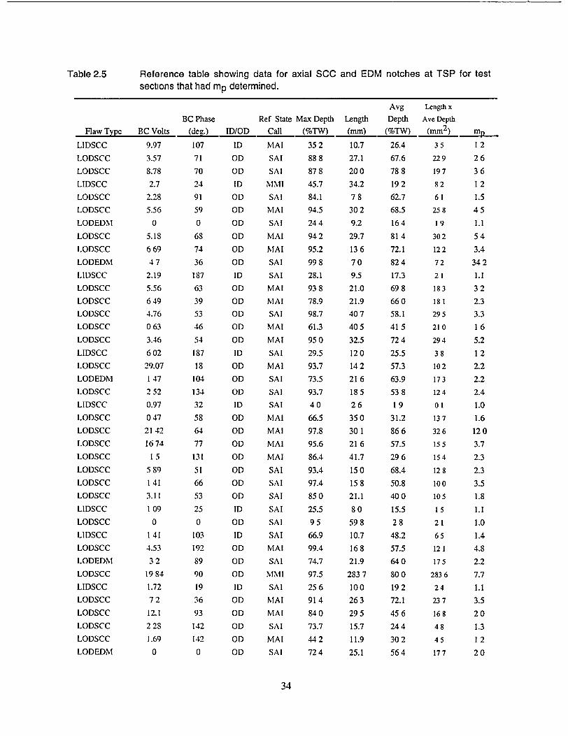
Reference table showing data for axial SCC and EDM notches at TSP for testsections that had mp determined.

Avg Length x

BC Phase Ref State Max Depth Length Depth Ave Depth

Flaw Type BC Volts (deg.) ID/OD Call (%TW) (mm) (%TW) (mm2 ) mp

LIDSCC 9.97 107 ID MAI 352 10.7 26.4 3 5 1 2

LODSCC 3.57 71 OD SAT 888 27.1 67.6 229 26

LODSCC 8.78 70 OD SA! 878 200 788 197 36

LIDSCC 2.7 24 ID MMI 45.7 34.2 192 82 1 2

LODSCC 2.28 91 OD SAI 84.1 78 62.7 61 1.5

LODSCC 5.56 59 OD MAI 94.5 302 68.5 25 8 4 5

LODEDM 0 0 OD SAT 244 9.2 164 19 1.1

LODSCC 5.18 68 OD MAI 942 29.7 814 302 54

LODSCC 669 74 OD MAI 95.2 136 72.1 122 3.4

LODEDM 47 36 OD SAT 998 70 824 72 342

LIDSCC 2.19 187 ID SAI 28.1 9.5 17.3 2 1 1.1

LODSCC 5.56 63 OD MAI 938 21.0 698 183 32

LODSCC 649 39 OD MAI 78.9 21.9 660 18 1 2.3

LODSCC 4.76 53 OD SAl 98.7 407 58.1 295 3.3

LODSCC 063 46 OD MAI 61.3 405 415 21 0 16

LODSCC 3.46 54 OD MAI 95 0 32.5 72 4 294 5.2

LIDSCC 602 187 ID SAT 29.5 120 25.5 3 8 12

LODSCC 29.07 18 OD MAI 93.7 142 57.3 102 2.2

LODEDM 147 104 OD SAI 73.5 216 63.9 173 2.2

LODSCC 252 134 OD SAl 93.7 185 538 124 2.4

LIDSCC 0.97 32 ID SAl 40 26 19 01 1.0

LODSCC 047 58 OD MAI 66.5 350 31.2 137 1.6

LODSCC 2142 64 OD MAI 97.8 301 866 326 120

LODSCC 1674 77 OD MAI 95.6 216 57.5 155 3.7

LODSCC 1 5 131 OD MAI 86.4 41.7 29 6 154 2.3

LODSCC 589 51 OD SAL 93.4 150 68.4 128 2.3

LODSCC 1 41 66 OD SAl 97.4 158 50.8 100 3.5

LODSCC 3.11 53 OD SAI 850 21.1 400 105 1.8

LIDSCC 1 09 25 ID SAI 25.5 80 15.5 1 5 1.1

LODSCC 0 0 OD SAl 95 598 28 21 1.0

LIDSCC 1 41 103 ID SAl 66.9 10.7 48.2 65 1.4

LODSCC 4.53 192 OD MAI 99.4 16 8 57.5 12 1 4.8

LODEDM 32 89 OD SAL 74.7 21.9 640 175 2.2

LODSCC 19 84 90 OD MMI 97.5 283 7 800 283 6 7.7

LIDSCC 1.72 19 ID SAl 256 100 192 24 1.1

LODSCC 7 2 36 OD MAI 914 263 72.1 237 3.5

LODSCC 12.1 93 OD MAI 840 295 456 168 20

LODSCC 228 142 OD SAl 73.7 15.7 244 48 1.3

LODSCC 1.69 142 OD MAI 442 11.9 302 45 12

LODEDM 0 0 OD SAI 724 25.1 564 177 20

34

Table 2.5

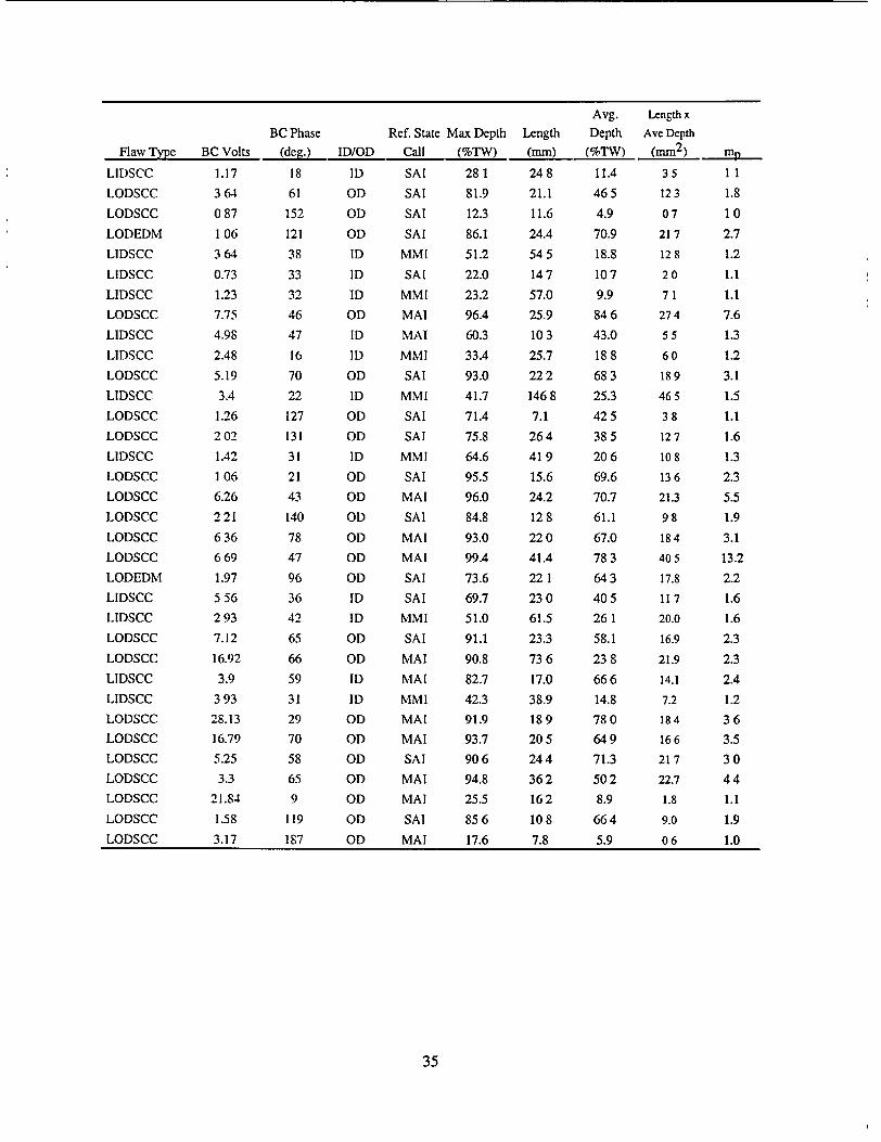
Avg. Length x BC Phase Ref. State Max Depth Length Depth Ave Depth

Flaw Type BC Volts (deg.) ID/OD Call (%TW) (mm) (%TW) (mm2 ) mp

LIDSCC 1.17 18 ID SAI 281 248 11.4 35 1 1

LODSCC 364 61 OD SAI 81.9 21.1 465 123 1.8

LODSCC 087 152 OD SAT 12.3 11.6 4.9 07 10

LODEDM 1 06 121 OD SAI 86.1 24.4 70.9 21 7 2.7

LIDSCC 3 64 38 ID MMI 51.2 545 18.8 128 1.2

LIDSCC 0.73 33 ID SAl 22.0 147 107 20 1.1

LIDSCC 1.23 32 ID MMI 23.2 57.0 9.9 7 1 1.1

LODSCC 7.75 46 OD MAI 96.4 25.9 84 6 274 7.6

LIDSCC 4.98 47 ID MAI 60.3 103 43.0 55 1.3

LIDSCC 2.48 16 ID MMI 33.4 25.7 18 8 60 1.2

LODSCC 5.19 70 OD SAI 93.0 222 683 189 3.1

LIDSCC 3.4 22 ID MMI 41.7 1468 25.3 465 1.5

LODSCC 1.26 127 OD SAl 71.4 7.1 425 38 1.1

LODSCC 202 131 OD SAI 75.8 264 385 127 1.6

LIDSCC 1.42 31 ID MMI 64.6 419 206 108 1.3

LODSCC 1 06 21 OD SAT 95.5 15.6 69.6 136 2.3

LODSCC 6.26 43 OD MAI 96.0 24.2 70.7 21.3 5.5

LODSCC 221 140 OD SAI 84.8 128 61.1 98 1.9

LODSCC 636 78 OD MAI 93.0 220 67.0 184 3.1

LODSCC 669 47 OD MAI 99.4 41.4 783 405 13.2

LODEDM 1.97 96 OD SAl 73.6 22 1 643 17.8 2.2

LIDSCC 556 36 ID SAl 69.7 230 405 117 1.6

LIDSCC 293 42 ID MMI 51.0 61.5 261 20.0 1.6

LODSCC 7.12 65 OD SAl 91.1 23.3 58.1 16.9 2.3

LODSCC 16.92 66 OD MAI 90.8 73 6 23 8 21.9 2.3

LIDSCC 3.9 59 ID MAI 82.7 17.0 666 14.1 2.4

LIDSCC 3 93 31 ID MMI 42.3 38.9 14.8 7.2 1.2

LODSCC 28.13 29 OD MAI 91.9 189 780 184 36

LODSCC 16.79 70 OD MAI 93.7 205 649 166 3.5

LODSCC 5.25 58 OD SAT 906 244 71.3 217 30

LODSCC 3.3 65 OD MAI 94.8 362 50 2 22.7 44

LODSCC 21.84 9 OD MAI 25.5 162 8.9 1.8 1.1

LODSCC 1.58 119 OD SAl 85 6 108 664 9.0 1.9

LODSCC 3.17 187 OD MAI 17.6 7.8 5.9 06 1.0

35

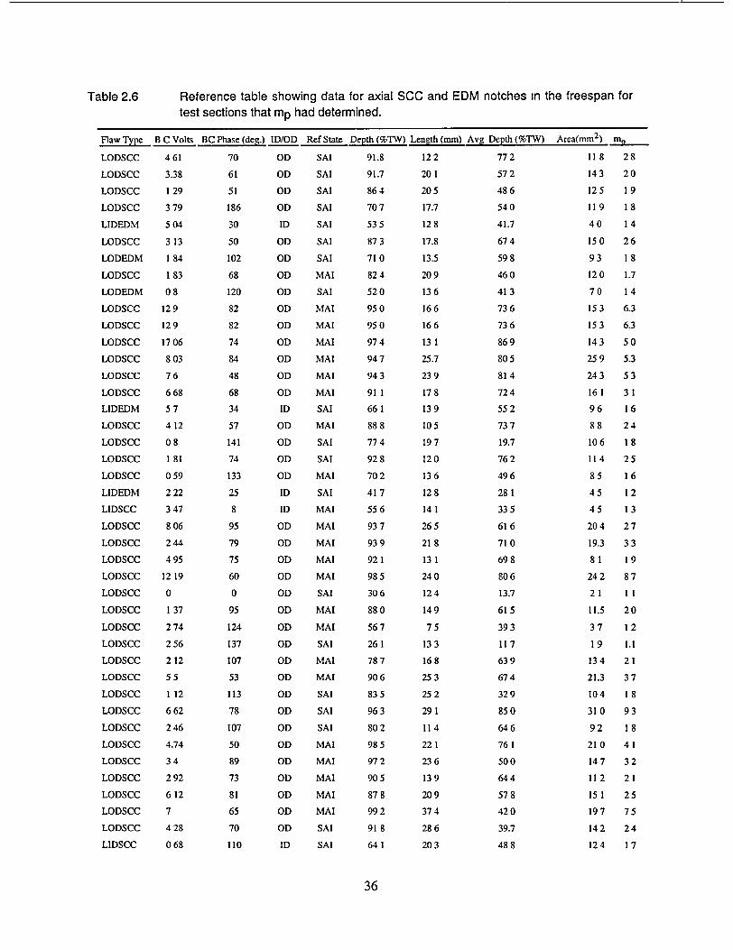
Table 2.6 Reference table showing data for axial SCC and EDM notches in the freespan for test sections that mp had determined.

Flaw Type B C Volts BC Phase (deg.) ID/OD Ref State Depth (%TW) Length (ram) Avg Depth (%TW) Area(mm2) M.

LODSCC 461 70 OD SAl 91.8 122 772 118 28

LODSCC 3.38 61 OD SAl 91.7 201 572 143 20

LODSCC 1 29 51 OD SAl 864 205 486 125 19

LODSCC 379 186 OD SAl 707 17.7 540 119 18

LIDEDM 504 30 ID SAl 535 128 41.7 40 14

LODSCC 3 13 50 OD SAI 873 17.8 674 150 26

LODEDM 184 102 OD SAL 710 13.5 598 93 18

LODSCC 183 68 OD MAI 824 209 460 120 1.7

LODEDM 08 120 OD SAL 520 136 413 70 14

LODSCC 129 82 OD MAI 950 166 736 153 6.3

LODSCC 129 82 OD MAI 950 166 736 153 6.3

LODSCC 1706 74 OD MAI 974 131 869 143 50

LODSCC 803 84 OD MAI 947 25.7 805 259 5.3

LODSCC 76 48 OD MAI 943 239 814 243 53

LODSCC 668 68 OD MAI 911 178 724 16! 3 1

LIDEDM 57 34 ID SAl 661 139 552 96 16

LODSCC 412 57 OD MAI 888 105 737 88 24

LODSCC 08 141 OD SAl 774 197 19.7 106 18

LODSCC 181 74 OD SAl 928 120 762 114 25

LODSCC 059 133 OD MAI 702 136 496 85 16

LIDEDM 222 25 ID SAl 417 128 28 1 45 12

LIDSCC 347 8 ID MA! 556 141 335 45 13

LODSCC 806 95 OD MAI 937 265 616 204 27

LODSCC 244 79 OD MAI 939 218 710 19.3 33

LODSCC 495 75 OD MAI 921 131 698 8 1 19

LODSCC 1219 60 OD MAI 985 240 806 242 87

LODSCC 0 0 OD SAI 306 124 13.7 21 1 1

LODSCC 137 95 OD MAI 880 149 615 11.5 20

LODSCC 274 124 OD MAI 567 75 393 37 12

LODSCC 256 137 OD SAl 261 133 117 19 1.1

LODSCC 212 107 OD MAI 787 168 639 134 21

LODSCC 55 53 OD MAI 906 253 674 21.3 37

LODSCC 112 113 OD SAI 835 252 329 104 18

LODSCC 662 78 OD SAT 963 291 850 310 93

LODSCC 246 107 OD SAl 802 114 646 92 18

LODSCC 4.74 50 OD MAI 985 221 761 210 41

LODSCC 34 89 OD MAI 972 236 500 147 32

LODSCC 292 73 OD MAI 905 139 644 112 21

LODSCC 612 81 OD MAI 878 209 578 151 25

LODSCC 7 65 OD MAI 992 374 420 197 75

LODSCC 428 70 OD SAl 91 8 286 39.7 142 24

LIDSCC 068 110 ID SAl 641 203 488 124 17

36

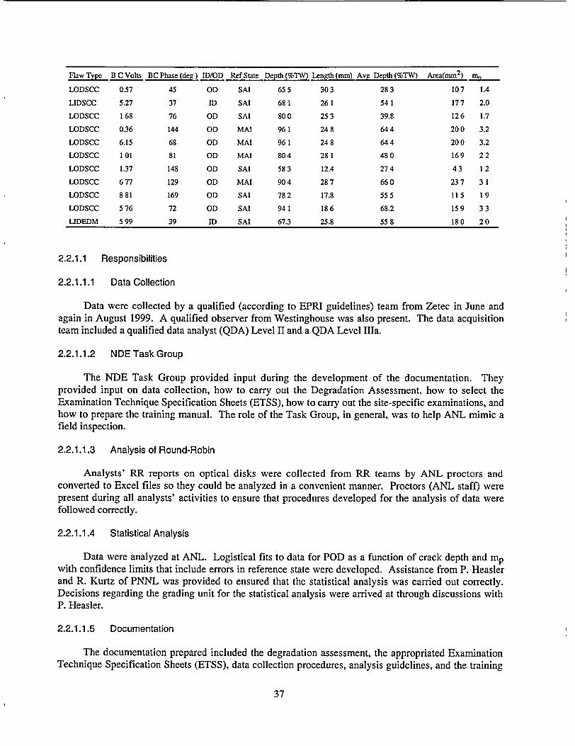
Flaw Type B C Volts BC Phase (deg) ID/OD Ref State Depth (%TW) Length (mm) Avg Depth (%TW) Area(mm 2 ) m__

LODSCC 0.57 45 OD SAt 655 303 283 107 1.4

LIDSCC 5.27 37 ID SAI 681 261 541 177 2.0

LODSCC 1 68 76 OD SAI 800 253 39.8 126 1.7

LODSCC 0.36 144 OD MAI 96 1 24 8 644 200 3.2

LODSCC 6.15 68 OD MAt 961 248 644 200 3.2

LODSCC 101 81 OD MAt 804 281 480 169 22

LODSCC 1.37 148 OD SAl 583 12.4 274 43 12

LODSCC 677 129 OD MAI 904 287 660 237 31

LODSCC 881 169 OD SAl 782 17.8 555 115 19

LODSCC 576 72 OD SAI 941 186 68.2 159 33

LIDEDM 599 39 ID SAI 67.3 25.8 558 180 20

2.2.1.1 Responsibilities

2.2.1.1.1 Data Collection

Data were collected by a qualified (according to EPRI guidelines) team from Zetec in June and again in August 1999. A qualified observer from Westinghouse was also present. The data acquisition team included a qualified data analyst (QDA) Level II and a QDA Level IIla.

2.2.1.1.2 NDE Task Group

The NDE Task Group provided input during the development of the documentation. They provided input on data collection, how to carry out the Degradation Assessment, how to select the Examination Technique Specification Sheets (ETSS), how to carry out the site-specific examinations, and how to prepare the training manual. The role of the Task Group, in general, was to help ANL mimic a field inspection.

2.2.1.1.3 Analysis of Round-Robin

Analysts' RR reports on optical disks were collected from RR teams by ANL proctors and converted to Excel files so they could be analyzed in a convenient manner. Proctors (ANL staff) were present during all analysts' activities to ensure that procedures developed for the analysis of data were followed correctly.

2.2.1.1.4 Statistical Analysis

Data were analyzed at ANL. Logistical fits to data for POD as a function of crack depth and mp with confidence limits that include errors in reference state were developed. Assistance from P. Heasler and R. Kurtz of PNNL was provided to ensured that the statistical analysis was carried out correctly. Decisions regarding the grading unit for the statistical analysis were arrived at through discussions with P. Heasler.

2.2.1.1.5 Documentation

The documentation prepared included the degradation assessment, the appropriated Examination Technique Specification Sheets (ETSS), data collection procedures, analysis guidelines, and the training

37

manual. Detailed documentation was prepared on how the RR exercise was carried out, the sequence of events, and the role of the ANL proctors, including administration of site-specific exams.

2.2.2 Round-Robin Documentation

Four documents were prepared for conduct of the mock-up testing and for the RR data analysis. They are ANLOO1 Rev. 2 "Argonne Analysis Guideline," ANL002 Rev. 3 "Multifrequency EC Examination of Tubing within the ANL SG Mock-up," ANL003 Rev. 3 "SG Mock-up Tubing Degradation Assessment and Technique Qualification," and ANL004 Rev. 3 "Training Manual." These documents are discussed below.

2.2.2.1 Degradation Assessment (ANL003 Rev. 3)

A Steam Generator Tube Degradation Assessment for flaws was prepared, per the requirements specified in NEI-97-06 and Revision 5 of the EPRI PWR Steam Generator Examination Guidelines. In accordance with Rev. 5 of the EPRI PWR Steam Generator Examination Guidelines, a review of EPRIqualified techniques was performed to ensure that application of these techniques was pertinent to sitespecific conditions of the mock-up.

This document identified the degradation mechanisms in the tubing of the steam generator mockup. This assessment also identified the inspection methods to be used to ensure that the inspection techniques and personnel used for the detection and sizing of tube flaws is appropriate for all degradation mechanisms. The training document for the RR addressed the handling of anomalous signals.

The degradation assessment reviewed all types of degradation in the mock-up, including the following:

(a) Intergranular attack (IGA) characterized by a uniform or relatively uniform attack of the grain boundaries over the surface of the tubing. When the occurrence is over a relatively large extent exhibiting three-dimensional features, the IGA is referred to as volumetric IGA. IGA is associated with the outside diameter of the tubing material. The IGA present in the mock-up is not mixed with SCC, a combination that can be found in the field and is easier to detect than pure IGA. However, the IGA in the mock-up is similar to that found in several operating plants. The mock-up IGA is representative of IGA at Cook, Point Beach, and San Onofre, simulating IGA found in the tube sheet crevice.

(b) Primary water stress corrosion cracking (PWSCC), defined as cracking that occurs on the tube's primary side (the inside diameter) when a source of stress is present in susceptible material. Locations of PWSCC in the mock-up include expansion transitions and dents.

(c) Wear, the volumetric removal of material caused by the mechanical action of one material in contact with another.

(d) Corrosive fatigue, which is a result of alternating stress cycles produced by tube vibration that may be accelerated by a corrosion process occurring during stress cycling. A few fatigue cracks can be found in the mock-up.

(e) Wastage that is corrosive wear to the outer wall of the tubing.

(f) Stress corrosion cracking initiating at the outer diameter (ODSCC) of Alloy 600 steam generator tubes is present at the TSP, in the freespan and in the tubesheet. ODSCC refers to a range of stress

38

corrosion cracking morphologies observed to occur along the OD of Alloy 600 steam generator tubing. Inspection requirements for this damage mechanism include 100% of the tube sheet transitions in Level A of the mock-up.

2.2.2.2 Data Acquisition Documentation (ANL002 Rev. 3)

The document "Multifrequency EC Examination of Tubing within the ANL SG Mock-up" provides all information necessary to collect the RR data. The procedures mimic those of an actual ISI. The basis of the data acquisition is the Examination Technique Specification Sheet (ETSS). The document defines the frequencies, axial and rotational speeds, and calibration procedures. Two ETSSs were developed for the ANL mock-up. These ETSSs are the result of reviewing EPRI ETSSs for the various degradation mechanisms in the mock-up and combining them into the two used.

One hundred percent of the tubes were inspected full-length with a bobbin coil. EPRI site-qualified technique ETSS 96008, covered by ANL's ETSS#1 (described later), was used. This technique has an EPRI-reported probability of detection of 85% at >40% TW at a confidence level of 90% in those areas not associated with the roll transition.

In addition, 100% of the tubes were inspected with a three-coil MRPC probe (Plus-PointTM, standard pancake and shielded high-frequency coil) at the top of tube sheet region. EPRI site-qualified technique ETSS 96403, covered by ANL's ETSS#2 (described later), was used for the detection of tube sheet flaws. This technique has an EPRI-reported probability of detection of 81% @ >50% TW at a 90% confidence level for both axial and circumferential indications.

Bobbin coil indications at TSPs were investigated with a rotating coil (Plus-PointTM). The sitequalified bobbin technique for nondented TSPs is EPRI ETSS 96007, covered by mock-up ETSS#1. The EPRI-reported probability of detection is 89% @ >60% TW at a 90% level of confidence. For all rotating coil inspections, site-qualified technique EPRI ETSS 96403, covered by mock-up ETSS#2, was used. This technique has an EPRI-reported probability of detection of 81% @ > 50% TW at a 90% confidence level for axial and circumferential indications.

The tubing in the mock-up steam generator was mechanically-expanded (rolled) in the shop. The transition zone is the region of the tube where the tube transitions from the expanded tube diameter to the nominal tube. Axial and circumferential indications are found in this region. A 100% rotating coil examination of top of the tube sheet was performed to detect PWSCC. EPRI site-qualified technique ETSS 96508, covered by mock-up ETSS#2, was used for detection of this degradation mechanism. This technique has an EPRI-reported probability of detection of 84% @ > 50% TW @ 90% confidence level for both axial and circumferential indications.

Corrosion of the TSPs causes the tubing to become dented, resulting in high localized stresses that lead to stress corrosion cracking. EPRI site-qualified Technique ETSS 96012 (covered by mock-up ETSS#1) was used for bobbin detection of axial PWSCC at TSP intersections (dent <2V). This technique has an EPRI-reported probability of detection of 89% @ >34% TW at a confidence level of 90%.

Site-qualified technique EPRI ETSS 96508 (covered by mock-up ETSS#2) was used for rotating coil detection of axial and circumferential PWSCC at dented locations and has an EPRI-reported probability of detection of 84% @ >50% TW at a confidence level of 90%.

39

Degradation due to wear is adequately identified by a bobbin coil examination. The technique used for detection of tube wear was EPRI ETSS 96004 (covered by mock-up ETSS#1) with an EPRI-reported probability of detection of 82% for >50% TW and a 90% confidence level.

No special examination requirements are listed in the EPRI PWR Steam Generator Examination Guidelines for fatigue degradation due to rapid growth rates.

Note that the EPRI-reported PODs may be determined from small sample sets, with the lower confidence limit the stated POD. As an example, if all cracks in a set of 11 test sections were detected (100% detection), the lower 90% confidence limit is 82% and the stated POD would be 0.82. EPRIstated PODs are adjusted to sample size.

2.2.2.3 ANL Analysis Guideline (ANL001 Rev. 3)

This procedure provided the technical direction for the performance of EC examinations of the ANL SG mock-up. This procedure was applicable to all examination personnel and generally mimics industry ISI guidelines. Flaws were located by data point. Percent throughwall was entered into the PERCENT column, with the exception of dents and dings. The three-letter analysis codes were entered into the UTIL1 column of the appropriate "Cal" record. Data were reviewed for the presence of undesirable noise with the following criteria: (a) Undesirable system noise was determined by identifying electrical interference or spiking associated with faulty probes, cabling and equipment. Studies have shown probe wear can generate undesirable horizontal noise resulting in poor signal-to-noise ratios. (b) Undesirable tube noise was determined by identifying signals caused by excessive permeability, pilgering, chatter, variations in tube geometry, tube cleanliness, and secondary-side sludge and deposits. These conditions were reported by the analyst so that a review could be performed to disposition these locations.

The primary and secondary analysts generated data used in the final analyst report and were responsible for reporting all indications. The resolution team (consisting of two resolution analysts and an independent QDA) performed the task of comparing and resolving discrepancies between the primary and secondary analyses. All identified differences in data interpretation were reviewed by resolution analysts to arrive at the final interpretation. The following procedures were used:

(a) If the primary and secondary analysts agreed that an indication is a flaw, it was reviewed by two resolution analysts. The independent QDA has the final say if there is no consensus on the call.

(b) If the primary and secondary analysts both give the "no detectable degradation" (NDD) call for a test section, there was no further analysis.

(c) If the primary and secondary analysts disagreed, the disagreement was resolved by the two resolution analysts. If the resolution analysts were not in agreement, the independent QDA made the final call.

Table 2.7 shows how the data from the analysts were recorded. The row and column of the test section was entered along with the voltage, phase angle, %TW, location by data point, three-letter code, and whether ID or OD.

40

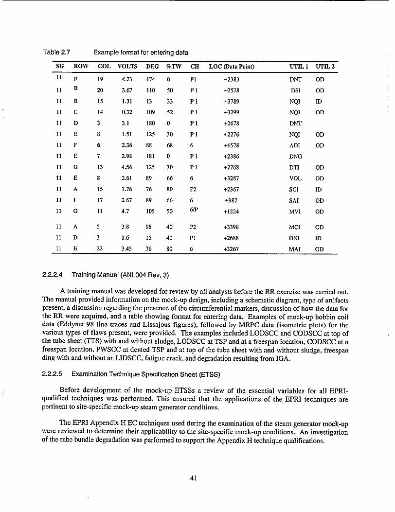
Table 2.7 Example format for entering data

SG ROW COL VOLTS DEG %TW CH LOC (Data Point) UTIL I UTIL 2

11 F 19 4.23 174 0 PI +2383 DNT OD 11 B 20 3.67 110 50 P1 +2578 DSI OD

11 B 15 1.31 13 33 P1 +3789 NQI ID

11 C 14 0.32 109 52 P1 +3299 NQI OD

11 D 3 3.1 180 0 P1 +2678 DNT

11 E 8 1.51 125 30 P1 +2276 NQI OD

11 F 6 2.36 88 68 6 +6578 ADI OD

11 E 7 2.98 181 0 P1 +2386 DNG

11 G 13 4.56 125 30 P1 +2768 DTI OD

11 E 8 2.61 89 66 6 +3287 VOL OD

I1 A 15 1.76 76 80 P2 +2367 SCI ID

11 I 17 267 89 66 6 +987 SAI OD

11 G 11 4.7 105 50 6/P +1224 MVI OD

11 A 5 3.8 98 40 P2 +3398 MCI OD

11 D 3 1.6 15 40 P1 +2688 DNI ID

11 B 22 3.45 76 80 6 +3267 MAI OD

2.2.2.4 Training Manual (ANL004 Rev. 3)

A training manual was developed for review by all analysts before the RR exercise was carried out. The manual provided information on the mock-up design, including a schematic diagram, type of artifacts present, a discussion regarding the presence of the circumferential markers, discussion of how the data for the RR were acquired, and a table showing format for entering data. Examples of mock-up bobbin coil data (Eddynet 98 line traces and Lissajous figures), followed by MRPC data (isometric plots) for the various types of flaws present, were provided. The examples included LODSCC and CODSCC at top of the tube sheet (TTS) with and without sludge, LODSCC at TSP and at a freespan location, CODSCC at a freespan location, PWSCC at dented TSP and at top of the tube sheet with and without sludge, freespan ding with and without an LIDSCC, fatigue crack, and degradation resulting from IGA.

2.2.2.5 Examination Technique Specification Sheet (ETSS)

Before development of the mock-up ETSSs a review of the essential variables for all EPRIqualified techniques was performed. This ensured that the applications of the EPRI techniques are pertinent to site-specific mock-up steam generator conditions.

The EPRI Appendix H EC techniques used during the examination of the steam generator mock-up were reviewed to determine their applicability to the site-specific mock-up conditions. An investigation of the tube bundle degradation was performed to support the Appendix H technique qualifications.

41

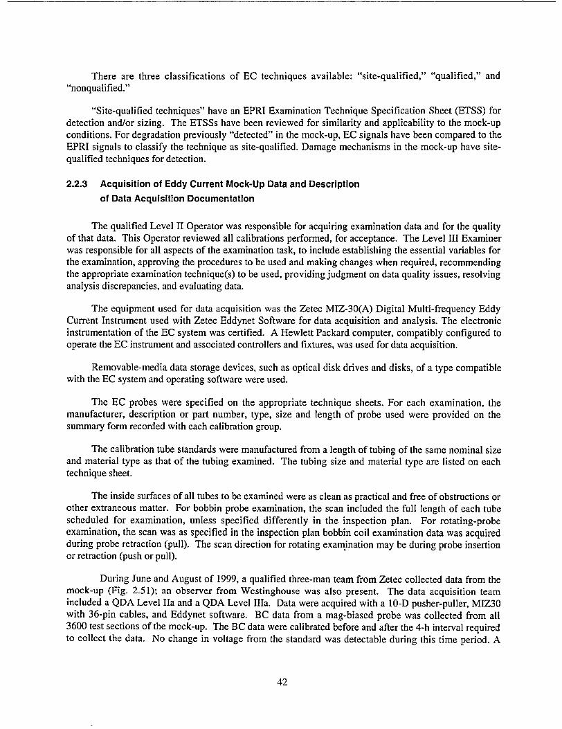
There are three classifications of EC techniques available: "site-qualified," "qualified," and "nonqualified."

"Site-qualified techniques" have an EPRI Examination Technique Specification Sheet (ETSS) for detection and/or sizing. The ETSSs have been reviewed for similarity and applicability to the mock-up conditions. For degradation previously "detected" in the mock-up, EC signals have been compared to the EPRI signals to classify the technique as site-qualified. Damage mechanisms in the mock-up have sitequalified techniques for detection.

2.2.3 Acquisition of Eddy Current Mock-Up Data and Description

of Data Acquisition Documentation

The qualified Level II Operator was responsible for acquiring examination data and for the quality of that data. This Operator reviewed all calibrations performed, for acceptance. The Level III Examiner was responsible for all aspects of the examination task, to include establishing the essential variables for the examination, approving the procedures to be used and making changes when required, recommending the appropriate examination technique(s) to be used, providing judgment on data quality issues, resolving analysis discrepancies, and evaluating data.

The equipment used for data acquisition was the Zetec MIZ-30(A) Digital Multi-frequency Eddy Current Instrument used with Zetec Eddynet Software for data acquisition and analysis. The electronic instrumentation of the EC system was certified. A Hewlett Packard computer, compatibly configured to operate the EC instrument and associated controllers and fixtures, was used for data acquisition.

Removable-media data storage devices, such as optical disk drives and disks, of a type compatible with the EC system and operating software were used.

The EC probes were specified on the appropriate technique sheets. For each examination, the manufacturer, description or part number, type, size and length of probe used were provided on the summary form recorded with each calibration group.

The calibration tube standards were manufactured from a length of tubing of the same nominal size and material type as that of the tubing examined. The tubing size and material type are listed on each technique sheet.

The inside surfaces of all tubes to be examined were as clean as practical and free of obstructions or other extraneous matter. For bobbin probe examination, the scan included the full length of each tube scheduled for examination, unless specified differently in the inspection plan. For rotating-probe examination, the scan was as specified in the inspection plan bobbin coil examination data was acquired during probe retraction (pull). The scan direction for rotating examination may be during probe insertion or retraction (push or pull).

During June and August of 1999, a qualified three-man team from Zetec collected data from the mock-up (Fig. 2.51); an observer from Westinghouse was also present. The data acquisition team included a QDA Level Ila and a QDA Level IIIa. Data were acquired with a 10-D pusher-puller, MIZ30 with 36-pin cables, and Eddynet software. BC data from a mag-biased probe was collected from all 3600 test sections of the mock-up. The BC data were calibrated before and after the 4-h interval required to collect the data. No change in voltage from the standard was detectable during this time period. A

42

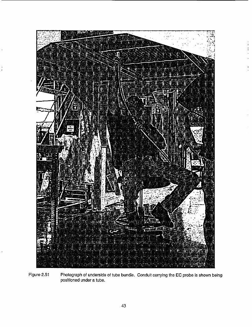
.1

I �t

r -�

U

Figure 2.51 Photograph of underside of tube bundle. Conduit carrying the EC probe is shown being positioned under a tube.

43

magnetically biased rotating three-coil probe that includes a +Point, 2.9-mm (0.1 15-in.)-diameter pancake and high-frequency shielded coil was used to collect data from all 400 tube sheet test sections and all special-interest (spin call) test sections. A comparison of magnetically biased and unbiased coils shows that the biasing eliminates the voltage shift and noise in the +Point EC signal resulting from tube sensitization.

The BC data were taken at 21 in./s, maintaining a digitization rate of 37 samples per inch. Bobbin coil data were taken at 400, 200, 100, and 20 kHz (differential and absolute). MRPC data was taken from all degraded test sections in addition to hundreds of clean test sections and test sections with artifacts. An ASME standard and a standard with 18 ID and OD axial and circumferential EDM notches (20, 40, 60, 80, and 100% throughwall) were used for calibration. MRPC data were taken at 900 rpm and an axial speed of 0.5 in./s (12.7 mm/s) to maintain a digitization rate of 30 samples per inch (12 samples/cm) in the circumferential direction and 30 in the axial direction. Data were taken at 600, 400, 300, 200, and 100 kHz. A total of nine +Point probes were used during this exercise because of probe wear. MRPC probes were replaced when one of the channels could not be nulled. This inability to null appears on the computer screen as an alert "flag."

All data were recorded on 2.6-GB magneto-optical disks. Two copies of the master disk were made, and all the data were copied to an ANL archive computer backup system. The setup for the bobbin coil and +Point probe matches or exceeds the specifications of the examination technique specification sheets (ETSSs) qualified for the flaws in the tube bundle.

The mock-up data collected by Zetec were analyzed at ANL (by ANL personnel) with Eddynet98 software. The locations of the flaw signals were checked against the location data of the flaw map. Locations of possible dings due to assembly that could lead to significant EC signals were noted. These dings could be created if a test section were inadvertently pressed against the simulated TSP during assembly.

During summer 1999, a recognized industry expert reviewed the ANL steam generator mock-up bobbin coil data and some of the MRPC data acquired by Zetec. The overall quality of the data was judged to be good, generally representative of field data and meeting or exceeding requirements for qualified techniques. For IGA, the examples in the mock-up are pure IGA, and not mixed with other cracks. The mock-up IGA is representative of IGA at Cook, Point Beach, and San Onofre, simulating IGA found in the tube sheet crevice. As a result of this data review, important knowledge on how to prepare the site-training document was acquired.

2.2.4 Examination Technique Specification Sheets

The Examination Technique Specification Sheets (ETSSs) developed for the RR are shown below. There are two ETSSs, one for the bobbin coil and one for the three-coil MRPC, which includes a mid-range +Point coil. The ETSSs provide the parameters for collecting and analyzing the RR data.

2.2.5 Participating Companies and Organization of Team Members

Companies participating in the RR provided a list of analysts who would be available to participate. For those companies who supplied more names than would be needed, ANL selected the team members by random picks from the list provided. The team members were expected to be available during the entire exercise, generally seven to eight working days. Analysts were generally QDA Level II-a or III.

44

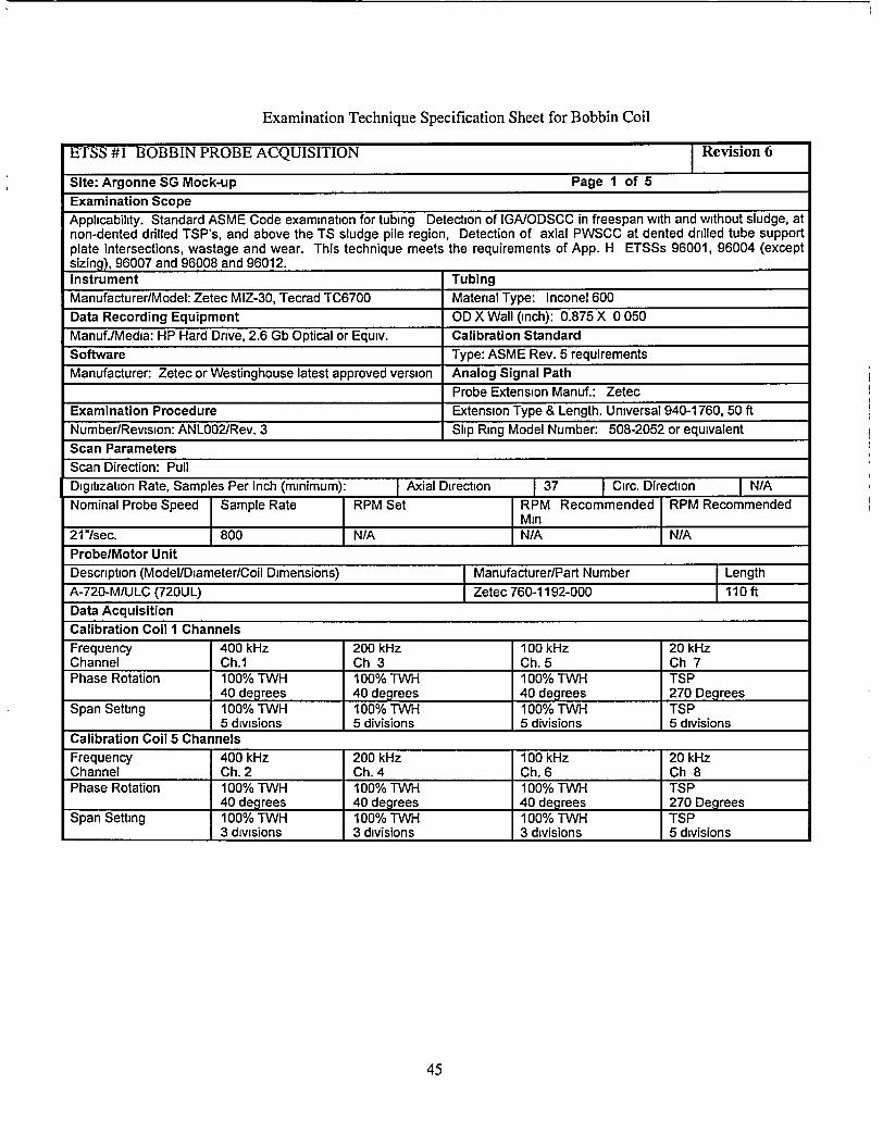
Examination Technique Specification Sheet for Bobbin Coil

ETSS #1 BOBBIN PROBE ACQUISITION Revision 6

Site: Argonne SG Mock-up Page 1 of 5 Examination Scope Applicability. Standard ASME Code examination for tubing Detection of IGAIODSCC in freespan with and without sludge, at non-dented drilled TSP's, and above the TS sludge pile region, Detection of axial PWSCC at dented drilled tube support plate intersections, wastage and wear. This technique meets the requirements of App. H ETSSs 96001, 96004 (except sizing), 96007 and 96008 and 96012. Instrument Tubing Manufacturer/Model: Zetec MIZ-30, Tecrad TC6700 Material Type: Inconel 600 Data Recording Equipment OD X Wall (inch): 0.875 X 0 050 Manuf./Media: HP Hard Dnve, 2.6 Gb Optical or Equiv. Calibration Standard Software Type: ASME Rev. 5 requirements Manufacturer: Zetec or Westinghouse latest approved version Analog Signal Path

Probe Extension Manuf.: Zetec Examination Procedure Extension Type & Length. Universal 940-1760, 50 ft Number/Revision: ANL002/Rev. 3 Slip Ring Model Number: 508-2052 or equivalent Scan Parameters Scan Direction: Pull Digitization Rate, Samples Per Inch (minimum): Axial Direction 37 Circ. Direction N/A Nominal Probe Speed Sample Rate RPM Set RPM Recommended RPM Recommended

Min

21"/sec. 800 N/A N/A N/A Probe/Motor Unit Description (Model/Diameter/Coil Dimensions) Manufacturer/Part Number Length A-720-M/ULC (720UL) Zetec 760-1192-000 110 ft Data Acquisition Calibration Coil I Channels Frequency 400 kHz 200 kHz 100 kHz 20 kHz Channel Ch.1 Ch 3 Ch. 5 Ch 7 Phase Rotation 100% TWH 100% TWH 100% TWH TSP

40 degrees 40 degrees 40 degrees 270 Degrees Span Setting 100% TWH 100% TWH 100% TWH TSP

5 divisions 5 divisions 5 divisions 5 divisions Calibration Coil 5 Channels Frequency 400 kHz 200 kHz 100 kHz 20 kHz Channel Ch. 2 Ch. 4 Ch. 6 Ch 8 Phase Rotation 100% TWH 100% TWH 100% TWVH TSP

40 degrees 40 degrees 40 degrees 270 Degrees Span Setting 100% TWH 100% TWH 100% TWH TSP

3 divisions 3 divisions 3 divisions 5 divisions

45

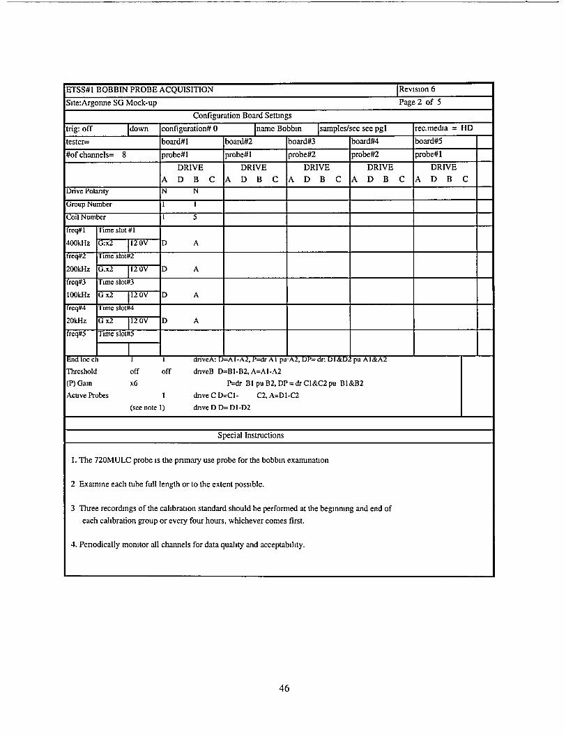
ETSS#1 BOBBIN PROBE ACQUISITION Revision 6

Site:Argonne SG Mock-up Page 2 of 5

Configuration Board Settings

trig: off Idown configuration# 0 name Bobbin samples/sec see pgl rec.media = HD

tester=- board#1 board#2 board#3 board#4 board#5

#of channels= 8 probe#1 probe#1 probe#2 probe#2 probe#1

DRIVE DRIVE DRIVE DRIVE DRIVE

A D B C A D B C A D B C A D B C A D BC Dnve Polarity N N

Group Number i

Coil Number 1 5

freq#I Time slot #1

400kHz G:x2 112 0V D A

freq#2 Time slot#2

200kHz G.x2 112 OV D A

freq#3 Time slot#3

100kHz G x2 112 0V D A

freq#4 Time slot#4

20kHz G x2 120V D A

freq#5 Time slot#5

End locbh 1 driveA: D=A I-A2, P=dr At pu'A2, DP= dr: D I &D2 pu A &A2

Threshold off off dnveB D=B1-B2, A=AI-A2

(P) Gain x6 P=dr BI pu B2, DP = dr Cl&C2 pu BI&B2

Active Probes I drive C D=Cl- C2, A=DI-C2

(see note 1) drive D D= DI-D2

Special Instructions

1. The 720MULC probe is the primary use probe for the bobbin examination

2 Examine each tube full length or to the extent possible.

3 Three recordings of the calibration standard should be performed at the beginning and end of

each calibration group or every four hours, whichever comes first.

4. Periodically monitor all channels for data quality and acceptability.

46

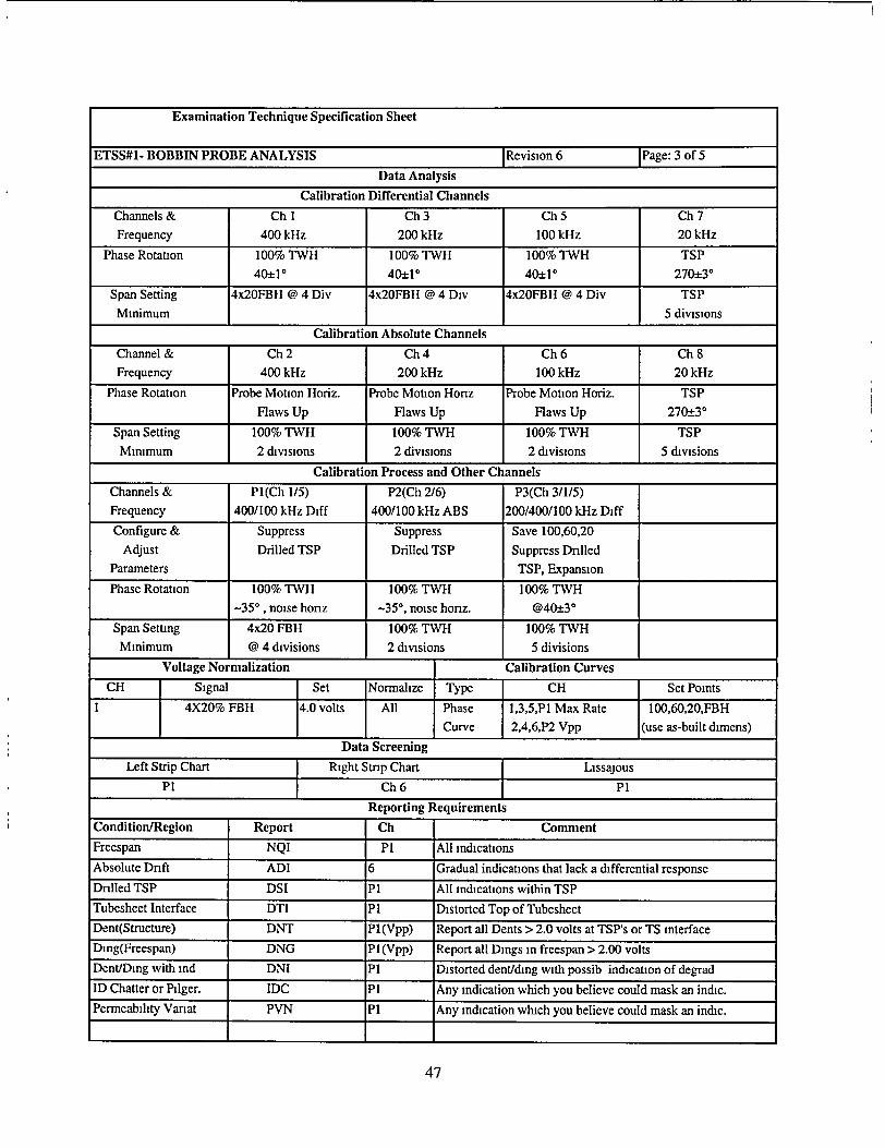
Examination Technique Specification Sheet

ETSS#1- BOBBIN PROBE ANALYSIS Revision 6 Page: 3 of 5

Data Analysis

Calibration Differential Channels

Channels & Ch 1 Ch3 Ch 5 Ch 7 Frequency 400 kHz 200 kHz 100 kHz 20 kHz

Phase Rotation 100% TWH 100% T"VH 100% TWH TSP

40±10 40±10 40±10 270±30

Span Setting 4x20FBH @ 4 Div 4x2OFBH @ 4 Div 4x2OFBH @ 4 Div TSP

Minimum 5 divisions

Calibration Absolute Channels

Channel & Ch 2 Ch 4 Ch 6 Ch 8 Frequency 400 kHz 200 kHz 100 kHz 20 kHz

Phase Rotation Probe Motion Horiz. Probe Motion Honz Probe Motion Horiz. TSP

Flaws Up Flaws Up Flaws Up 270±30

Span Setting 100% TWH 100% TWH 100% TWH TSP

Minimum 2 divisions 2 divisions 2 divisions 5 divisions

Calibration Process and Other Channels

Channels & Pl(Ch 115) P2(Ch 2/6) P3(Ch 3/1/5) Frequency 400/100 kHz Diff 400/100 kHz ABS 200/400/100 kHz Diff

Configure & Suppress Suppress Save 100,60,20 Adjust Drilled TSP Drilled TSP Suppress Drilled

Parameters TSP, Expansion

Phase Rotation 100% TWH 100% TWH 100% TWH

-35' , noise honz -35*, noise honz. @40±3"

Span Setting 4x20 FBH 100% TWH 100% TWH Minimum @ 4 divisions 2 divisions 5 divisions

Voltage Normalization Calibration Curves

CH Signal Set Normalize Type CH Set Points

4X20% FBH 4.0 volts All Phase 1,3,5,P1 Max Rate 100,60,20,FBH

Curve 2,4,6,P2 Vpp (use as-built dimens)

Data Screening

Left Strip Chart Right Strip Chart Lissajous

PI Ch 6 P1

Reporting Requirements

Condition/Region Report Ch Comment

Freespan NQI PI All indications

Absolute Drift ADI 6 Gradual indications that lack a differential response

Drilled TSP DSI P1 All indications within TSP

Tubesheet Interface DTI P1 Distorted Top of Tubesheet

Dent(Structure) DNT P1(Vpp) Report all Dents > 2.0 volts at TSP's or TS interface

Ding(Freespan) DNG Pl(Vpp) Report all Dings in freespan > 2.00 volts

Dent/Ding with md DNI P1 Distorted dent/ding with possib indication of degrad

ID Chatter or Pilger. IDC P1 Any indication which you believe could mask an indic.

Permeability Variat PVN P1 Any indication which you believe could mask an indic.

47

48

Examination Technique Specification Sheet ETSS# 1- Bobbin Probe Analysis Revision 6 Page 4 of 5

Special Instructions

1. Provide a best estimate of %TW on all bobbin indications based on ASME calibration curve. Place appropriate "I-Code" in the Utility 1 field. Place flaw origin in Util 2 (ID or OD).

2. Zoom the strip charts to 3 (or equivalent setting based on window size) for increased visibility of small amplitude indications.

3. Scroll each freespan region with channel 3.

4. Scroll each top of tubesheet region and expansion transition with channel P1 and P3.

5. Review each drilled TSP with channel P1 and Channel 3.

6. Monitor the 100 kHz absolute strip chart for positive drift.

7. Refer to the flow chart on the following page for additional information on evaluation of indications.

8. When distorted indications within dents or dings are identified, record the dent voltage as well as the indication.

9. All data should be analyzed unless voided by the operator. There are no retest codes necessary for the mock-up. Use BDA for bad data.

10. Landmarking is not necessary. All elevations will be recorded by data point.

11. Graphics are not required.

12. Do not report signals within one inch of test section ends.

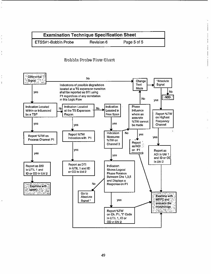
Examination Technique Specification Sheet

ETSS#1 -Bobbin Probe Revision 6 Page 5 of 5

49

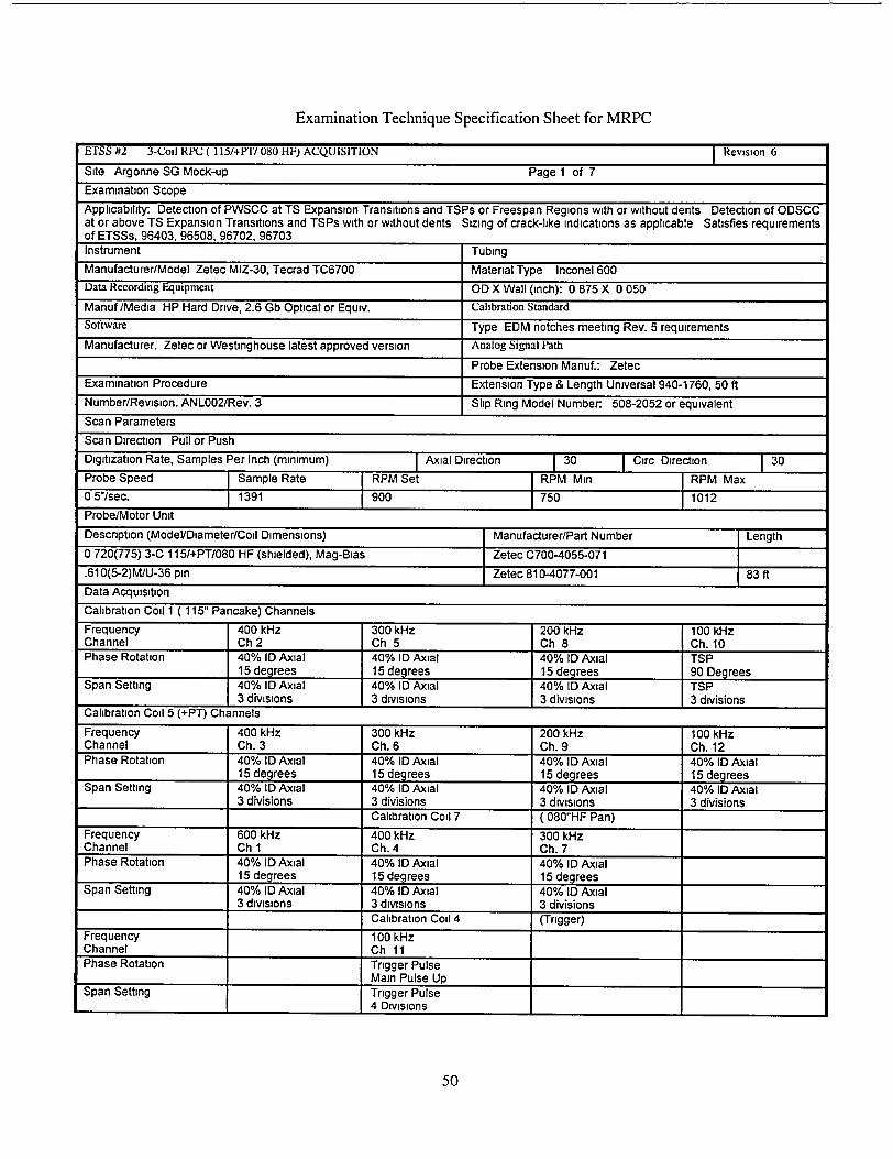
Examination Technique Specification Sheet for MRPC

ETSS #2 3-Cod RPC ( 115/+PTI/080 HF) ACQUISITION I Revision 6

Site Argonne SG Mock-up Page 1 of 7

Examination Scope

Applicability: Detection of PWSCC at TS Expansion Transitions and TSPs or Freespan Regions with or without dents Detection of ODSCC at or above TS Expansion Transitions and TSPs with or without dents Sizing of crack-like indications as applicable Satisfies requirements of ETSSs. 96403. 96508. 96702. 96703Instrument Tubing Manufacturer/Model Zetec MIZ-30, Tecrad TC6700 Material Type Inconel 600 Data Recording Equipment OD X Wall (inch): 0 875 X 0 050

Manuf/Media HP Hard Drive, 2.6 Gb Optical or Equiv. Calibration Standard Software Type EDM notches meeting Rev. 5 requirements Manufacturer. Zetec or Westinghouse latest approved version Analog Signal Path

Probe Extension Manuf.: Zetec Examination Procedure Extension Type & Length Universal 940-1760, 50 ft Number/Revision. ANLO02/Rev. 3 Slip Ring Model Number. 508-2052 or equivalent Scan Parameters

Scan Direction Pull or Push Digitization Rate, Samples Per Inch (minimum) - Axial Direction 30 Circ Direction 30 Probe Speed Sample Rate RPM Set RPM Mi RPM Max 0 5"/sec. 1391 900 750 1012 Probe/Motor Unit

Description (ModelI/Diamete r/Co il Dimensions) Manufacturer/Part Number Length 0 720(775) 3-C 115/+PT/080 HF (shielded), Mag-Bias Zetec C700-4055-071 .610(5-2)M/U-36 pin Zetec 810-4077-001 83 ft Data Acquisition Calibration Coil 1 ( 115" Pancake) Channels Frequency 400 kHz 300 kHz 200 kHz 100 kHz Channel Ch 2 Ch 5 Ch 8 Ch. 10 Phase Rotation 40% ID Axial 40% ID Axial 40% ID Axial TSP

15 degrees 15 degrees 15 degrees 90 Degrees Span Setting 40% ID Axial 40% ID Axial 40% ID Axial TSP

3 divisions 3 divisions 3 divisions 3 divisions Calibration Coil 5 (+PT) Channels Frequency 400 kHz 300 kHz 200 kHz 100 kHz Channel Ch. 3 Ch. 6 Ch. 9 Ch. 12 Phase Rotation 40% ID Axial 40% ID Axial 40% ID Axial 40% ID Axial

15 degrees 15 degrees 15 degrees 15 degrees Span Setting 40% ID Axial 40% ID Axial 40% ID Axial 40% ID Axial

3 divisions 3 divisions 3 divisions 3 divisions Calibration Coil 7 (080"HF Pan)

Frequency 600 kHz 400 kHz 300 kHz Channel Ch 1 Ch. 4 Ch. 7 Phase Rotation 40% ID Axial 40% ID Axial 40% ID Axial

15 degrees 15 degrees 15 degrees Span Setting 40% ID Axial 40% ID Axial 40% ID Axial

3 divisions 3 divisions 3 divisions Calibration Coil 4 (Trigger)

Frequency 100 kHz Channel Ch 11 Phase Rotation Trigger Pulse

Main Pulse Up Span Setting Trigger Pulse

4 Divisions

50

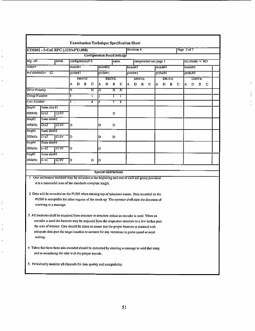
Examination Technique Specification Sheet

ETSS#2 - 3-Coil RPC (.115/+PT/.080) Revision 6 Page 2 of 7

Configuration Board Settings

trig off down conf0igration# 0 name samples/see:see page 1 rec.media = HD

tester=- board# I board#2 board#3 board#4 board#5

#of channels= 12 probe#l probe#l probe#3 probe#4 probe#5

DRIVE DRIVE DRIVE DRIVE DRIVE

A D B C A D B C A D B C A D B C A D B C

Drive Polarity N N N N N

Group Number I I I 1 1

Coil Number 1 4 5 7 8

freq#1I Time slot #1

600kHz G:x2 112 OV D

freq#2 Time slot#2

400kHz G:x2 112 0V D D D

freq#3 Time slot#3

300kHz G x2 112 0V D D

freq#4 Time slot#4

100kHz G x2 1120V D D

Special Instructions

I One calloration standard may be recorded at the beginning and end of each cal group provided it is a successful scan of the standards complete length.

2 Data will be recorded on the PUSH when running top of tubesheet exams Data recorded on the

PUSH is acceptable for other regions of the mock-up The operator shall state the direction of

scanning in a message.

3 All locations shall be acquired from structure to structure unless an encoder is used When an

encoder is used the location may be acquired from the respective structure to a few inches past

the area of interest. Care should be taken to insure that the proper location is scanned with

adequate data past the target location to account for any variations in probe speed or axial

scaling.

4 Tubes that have been mis-encoded should be corrected by entering a message to void that entry

and re-examimng the tube with the proper encode.

5. Periodically monitor all channels for data quality and acceptability.

51

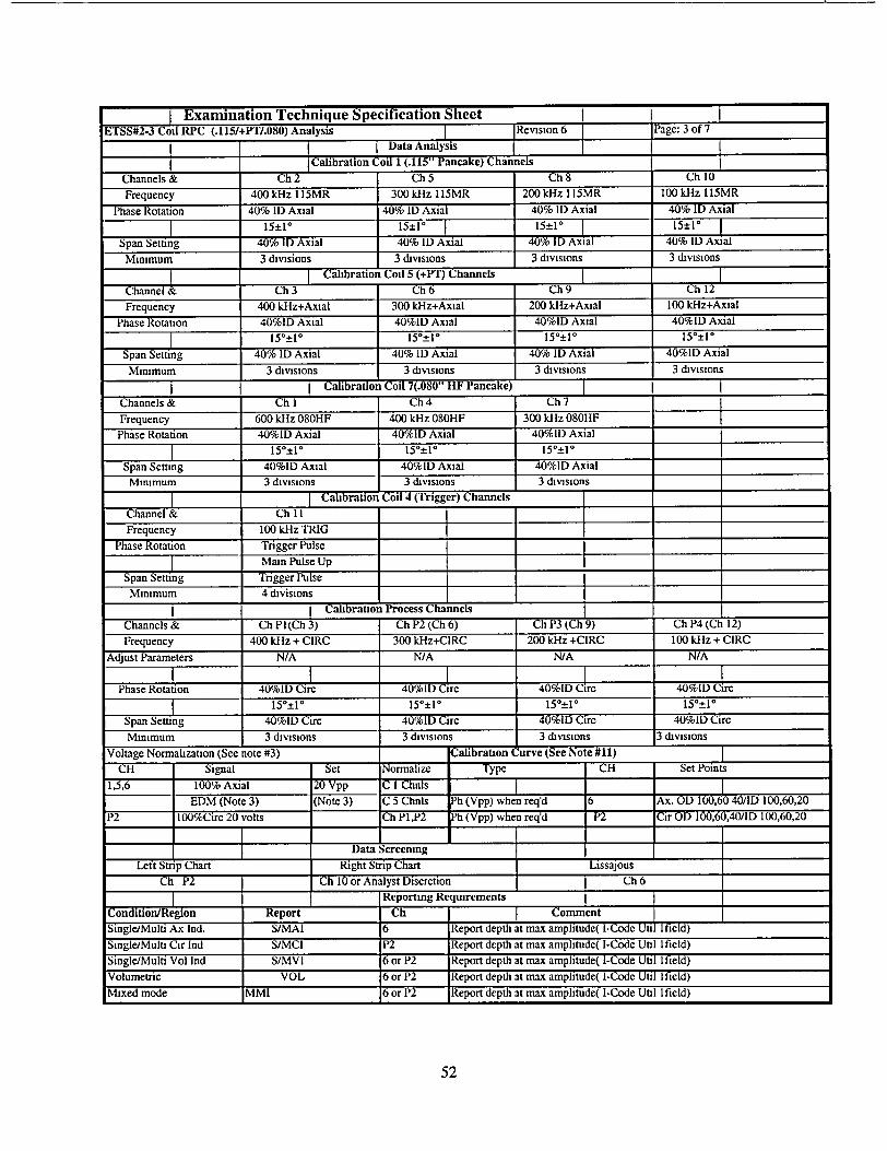
Examination Technique Specification Sheet ETSS#2-3 Coil RPC (.115/+PT/.080) Analysis tRevision 6e 3 of7

|Data Analysis

Calibration Coil 1 (.115" Pancake) Channels

Channels & Ch 2 Ch 5 Ch 8 Ch 10

Frequency 400 kHz 115MR 300 kHz 115MR 200 kHz 115MR 100 kHz 115MR

Phase Rotation 40% ID Axial 40% ID Axial 40% ID Axial 40% ID Axial

1* 10 1- 1° 15±1°5-+1 1 Span Setting 40% ID Axial 40% ID Axial 40% ID Axial 40% ID Axial

Minimum 3 divisions 3 divisions 3 divisions 3 divisions

ICalthration Coil 5 (+PT) Channels

Channel & Ch 3 Ch 6 Ch 9 Ch 12

Frequency 400 kHz+Axial 300 kHz+Axial 200 kHz+Axial 100 kHz+Axial

Phase Rotation 40%ID Axial 40%ID Axial 40%ID Axial 40%ID Axial

150±1 150±10 15_±10 150±10

Span Setting 40% ID Axial 40% ID Axial 40% ID Axial 40%1ID Axial

Minimum 3 divisions 3 divisions 3 divisions 3 divisions

ICalibration Coil 7(.080" IF Pancake)

Channels & Ch 1 Ch 4 Ch 7 Frequency 600 kHz 080HF 400 klHz 080HF 300 kHz 080HF

Phase Rotation 40%ID Axial 40%ID Axial 40%ID Axial

1 15±0 ± 150±10 150±10 Span Setting 40%LD Axial 40%ID Axial 40%ID Axial

Minimum 3 divisions 3 divisions 3 divisions

S T Calbration Coil 4 (Trigger) Channels Channel & Ch It Frequency 100 kHz TRIG

Phase Rotation Trigger Pulse Main Pulse Up

Span Setting Trigger Pulse

Minimum 4 divisions

I - 1 Cahbrat14 Process Channels _C 3C9h4(C 2 Channels & Ch PI(Ch 3) Ch P2 (Ch 6) CP3(h 9) hP4 Ch 12)

Frequency 400 kHz + CIRC 300 kHz+CIRC 200 kHz +CIRC 100 kHz + CIRC

Adjust Parameters N/A N/A N/A N/A

Phase Rotation 40%1D Circ 40%1D Circ 40%1ID Circ 40%1D Circ

150±10 150±10 150±10 150±10

Span Setting 40%ID Circ 40%ID Circ 40%ID Circ 40%ID Cire

Minimum 3 divisions 3 divisions 3 divisions 3 divisions

Voltage Normaahzation (See note #3) Calibration Curve (See Note #11)

CH Signal Set Normaize Type CH Set Points

1,76 - 100% Axial 20 Vpp C l Chnls

EDM (Note 3) (Note 3) C 5 Chnls Ph (Vpp) when req'd 6 Ax. OD 100,60 40/ID 100,60,20

P2 100%Circ 20 volts Ch Pl,P2 Ph (Vpp) when req'd P2 Cir OD 100,60,40/ID 100,60,20

Data Screening

Left Strip Chart Right Strip Chart Lissajous

Ch P2 Ch 10 or Analyst Discretion Ch 6 Iz = Reporting Requirements

C ioin/Region Report Ch Comment

Single/Multi Ax Ind. S/MAI 6 Report depth at max amplitude( 1-Code Util 1field)

Single/Multi Cir Ind S/MCI P2 Report depth at max amplitude( 1-Code Util Ifield)

Single/Multi Vol Ind S/MVI T or P2 Report depth at max amplitude( I-Code Util Ifield)

Volumetric VOL 6 or P2 Report depth at max amplitude( I-Code Util ifield)

Mixed mode MMI 6 or P2 Report depth at max amplitude( 1-Code Util Ifield)

52

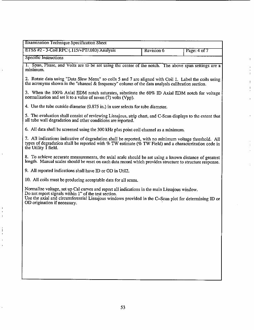
Examination Technique Specification Sheet

ETSS #2- 3-Coil RPC (.1 15/+PT/.080) Analysis Revision 6 I Page: 4 of 7 Specific Instructions

1. Span, Phase, and Volts are to be set using the center of the notch. The above span settings are a minimum.

2. Rotate data using "Data Slew Menu" so coils 5 and 7 are aligned with Coil 1. Label the coils using the acronyms shown in the "channel & frequency" column of the data analysis calibration section.

3. When the 100% Axial EDM notch saturates, substitute the 60% ID Axial EDM notch for voltage normalization and set it to a value of seven (7) volts (Vpp).

4. Use the tube outside diameter (0.875 in.) in user selects for tube diameter. 5. The evaluation shall consist of reviewing Lissajous, strip chart, and C-Scan displays to the extent that all tube wall degradation and other conditions are reported.

6. All data shall be screened using the 300 kHz plus point coil channel as a minimum.

7. All indications indicative of degradation shall be reported, with no minimum voltage threshold. All types of degradation shall be reported with % TW estimate (% TW Field) and a characterization code in the Utility 1 field.

8. To achieve accurate measurements, the axial scale should be set using a known distance of greatest length. Manual scales should be reset on each data record which provides structure to structure response.

9. All reported indications shall have ID or OD in Util2.

10. All coils must be producing acceptable data for all scans.

Normalize voltage, set up Cal curves and report all indications in the main Lissajous window. Do not report signals within 1" of the test section. Use the axial and circumferential Lissajous windows provided in the C-Scan plot for determining ID or OD origination if necessary.

53

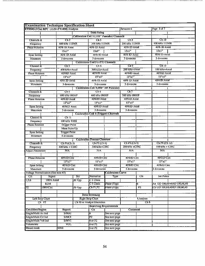
Examination Technique Specification SheetETSS#2-3 Coil RPC (.115/+PT/.080) Analysis IRevision 6 Page 5 of 7

Data Sizing Calibration Coil 1 (.115" Pancake) Channels

Channels & Ch2 Ch5 Ch 8 Ch 10

Frequency 400 kHz 115MR 300 kHz 115MR 200 kHz 115MR 100 kHz 1 ISMR

Phase Rotation 40% ID Axial 40% ID Axial 40% ID Axial 40% ID Axial

ý J I 15±10 15_1 1 15_1° 15±10

Span Setting 40% ID Axial 40% ID Axial 40% ID Axial 40% ID Axial

Minimum 3 divisions 3 divisions 3 divisions 3 divisions

IZ Cabration Coil 5 (+PT) Channels

Channel & Ch 3 Ch 6 Ch 9 Ch 12

Frequency 400 kHz+Axial 300 kHz+Axial 200 kHz+Axial 100 kHz+Axial

Phase Rotation 40%ID Axial 40%lD Axial 40%ID Axial 40%ID Axial 15°±10 150±+10 15°_±10 150±1

Span Setting 40% ID Axial 40% ID Axial 40% ID Axial 40%ID Axial

Minimum 3 divisions 3 divisions 3 divisions 3 divisions

SCalibration Coil 7(.080'" 1F Pancake)

Channels & Ch I Ch 4 Ch 7 Frequency 600 kHz 080HF 400 kHz 080HF 300 kHz 080HF

Phase Rotation 40%ID Axial 40%ID Axial 40%ID Axial

I 150±10 150±10 150±10* Span Setting 40%ID Axial 40%ID Axial 40%ID Axial

Minimum 3 divisions 3 divisions 3 divisions

I I Calibration Coil 4 (Trigger) Channels Channel & Ch 11

Frequency 100 kHz TRIG Phase Rotation Trigger Pulse

Main Pulse Up Span Setting Trigger Pulse Minimum 4 divisions

a ibration Process Channels

Channels & Ch PI(Ch 3) Ch P2 (Ch 6) Ch P3 (Ch 9) Ch P4 (Ch 12)

Frequency 400 kHz + CIRC 300 kHz+CIRC 200 kHz +CIRC 100 kHz + CIRC

Adjust Parameters N/A N/A N/A N/A

Phase Rotation 40%1iD Circ 40%1D Circ 40%1D Circ 40%ID Cire

150±10 150±+10 150±10 150±10

Span Setting 40%ID Circ 40%ID Circ 40%ID Circ 40%1D Circ

Minimum 3 divisions 3 divisions 3 divisions 3 divisions

Voltage Normalization (See note #3) Calibration Curve

CH Signal Set Normalize Type CH Set Points

1,5,6 100% Axial 20 Vpp C I Chnls EDM C 5 Chnls Phase (Vpp) 6 Ax OD 100,60 40/ID 100,60,40

P2 100%Circ 20 Vpp Ch PI,P2 Phase (Vpp) P2 Cir OD 100,60,40/ID 100,60,40

1 ~Data ScreeningI

Left Strip Chart ght Strip Chart Lissajous

Ch P2 Ch I0 or Analyst Discretion Ch 6 [ Reporting Requirements

Condition/Region Report Ch Comment

Single/Multi Ax Ind S/MAI 6 See next page

Single/Multi Cir Ind S/MCi P2 See next page Single/Multi Vol Ind S/MVI 6 or P2 See next page

Volumetric VOL 6 or P2 See next page

Mixed mode MMI 6 or P2 See next page

54

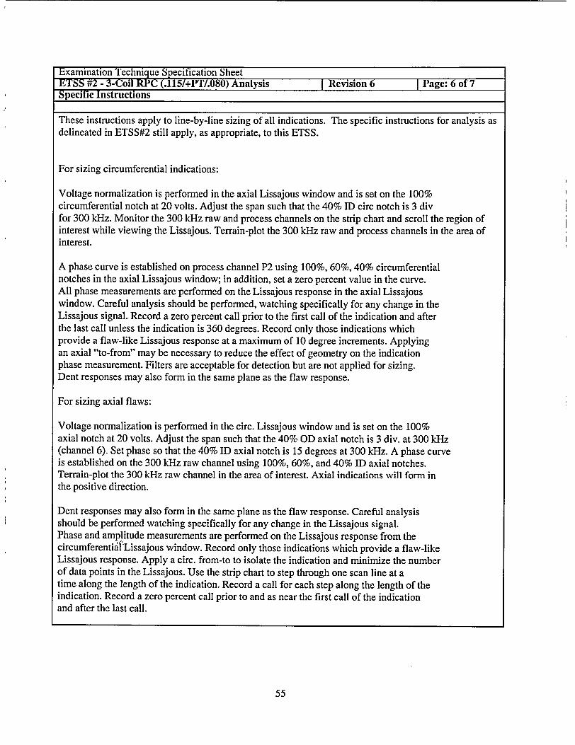
Examination Technique Specification Sheet ETSS #2 - 3-Coil RPC (.l15/+PT/.080) Analysis Revision 6 Page: 6 of 7 Specific Instructions

These instructions apply to line-by-line sizing of all indications. The specific instructions for analysis as delineated in ETSS#2 still apply, as appropriate, to this ETSS.

For sizing circumferential indications:

Voltage normalization is performed in the axial Lissajous window and is set on the 100% circumferential notch at 20 volts. Adjust the span such that the 40% ID circ notch is 3 div for 300 kHz. Monitor the 300 kHz raw and process channels on the strip chart and scroll the region of interest while viewing the Lissajous. Terrain-plot the 300 kHz raw and process channels in the area of interest.

A phase curve is established on process channel P2 using 100%, 60%, 40% circumferential notches in the axial Lissajous window; in addition, set a zero percent value in the curve. All phase measurements are performed on the Lissajous response in the axial Lissajous window. Careful analysis should be performed, watching specifically for any change in the Lissajous signal. Record a zero percent call prior to the first call of the indication and after the last call unless the indication is 360 degrees. Record only those indications which provide a flaw-like Lissajous response at a maximum of 10 degree increments. Applying an axial "to-from" may be necessary to reduce the effect of geometry on the indication phase measurement. Filters are acceptable for detection but are not applied for sizing. Dent responses may also form in the same plane as the flaw response.

For sizing axial flaws:

Voltage normalization is performed in the circ. Lissajous window and is set on the 100% axial notch at 20 volts. Adjust the span such that the 40% OD axial notch is 3 div. at 300 kHz (channel 6). Set phase so that the 40% ID axial notch is 15 degrees at 300 kHz. A phase curve is established on the 300 kHz raw channel using 100%, 60%, and 40% ID axial notches. Terrain-plot the 300 kHz raw channel in the area of interest. Axial indications will form in the positive direction.

Dent responses may also form in the same plane as the flaw response. Careful analysis should be performed watching specifically for any change in the Lissajous signal. Phase and amplitude measurements are performed on the Lissajous response from the circumferentiAv-Lissajous window. Record only those indications which provide a flaw-like Lissajous response. Apply a circ. from-to to isolate the indication and minimize the number of data points in the Lissajous. Use the strip chart to step through one scan line at a time along the length of the indication. Record a call for each step along the length of the indication. Record a zero percent call prior to and as near the first call of the indication and after the last call.

55

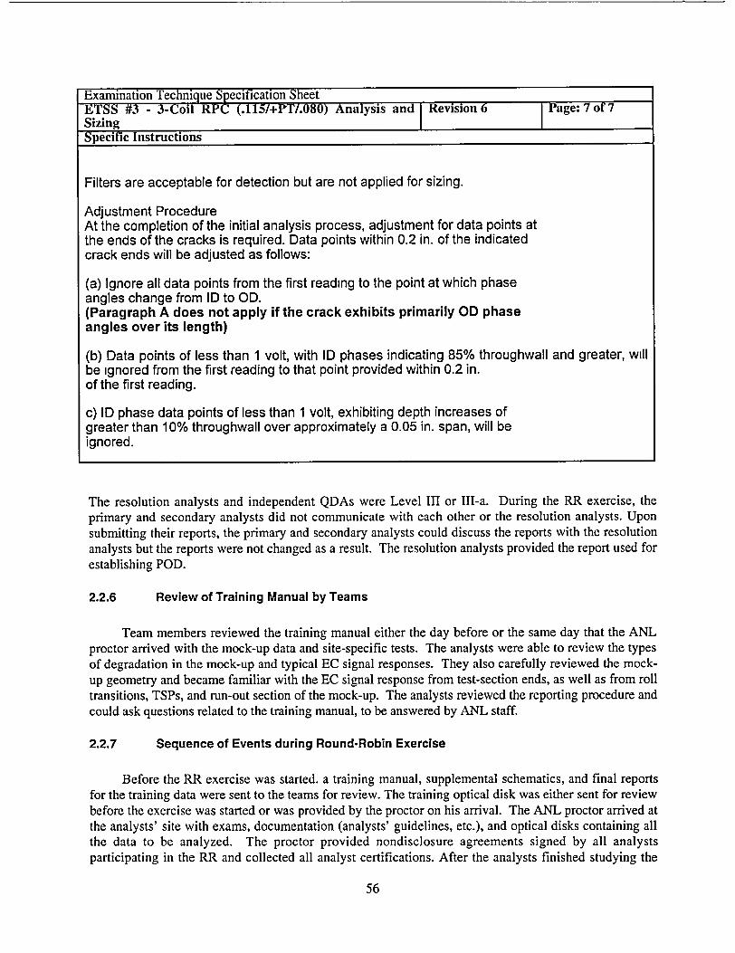
The resolution analysts and independent QDAs were Level III or III-a. During the RR exercise, the primary and secondary analysts did not communicate with each other or the resolution analysts. Upon submitting their reports, the primary and secondary analysts could discuss the reports with the resolution analysts but the reports were not changed as a result. The resolution analysts provided the report used for establishing POD.

2.2.6 Review of Training Manual by Teams

Team members reviewed the training manual either the day before or the same day that the ANL proctor arrived with the mock-up data and site-specific tests. The analysts were able to review the types of degradation in the mock-up and typical EC signal responses. They also carefully reviewed the mockup geometry and became familiar with the EC signal response from test-section ends, as well as from roll transitions, TSPs, and run-out section of the mock-up. The analysts reviewed the reporting procedure and could ask questions related to the training manual, to be answered by ANL staff.

2.2.7 Sequence of Events during Round-Robin Exercise

Before the RR exercise was started. a training manual, supplemental schematics, and final reports for the training data were sent to the teams for review. The training optical disk was either sent for review before the exercise was started or was provided by the proctor on his arrival. The ANL proctor arrived at the analysts' site with exams, documentation (analysts' guidelines, etc.), and optical disks containing all the data to be analyzed. The proctor provided nondisclosure agreements signed by all analysts participating in the RR and collected all analyst certifications. After the analysts finished studying the

56

Examination Technique Specification Sheet ETSS #3 - 3-Coil RPC (.115/+PT/.080) Analysis and I Revision 6 I Page: 7 of 7 Sizing I Specific Instructions

Filters are acceptable for detection but are not applied for sizing.

Adjustment Procedure At the completion of the initial analysis process, adjustment for data points at the ends of the cracks is required. Data points within 0.2 in. of the indicated crack ends will be adjusted as follows:

(a) Ignore all data points from the first reading to the point at which phase angles change from ID to OD. (Paragraph A does not apply if the crack exhibits primarily OD phase angles over its length)

(b) Data points of less than 1 volt, with ID phases indicating 85% throughwall and greater, will be ignored from the first reading to that point provided within 0.2 in. of the first reading.

c) ID phase data points of less than 1 volt, exhibiting depth increases of greater than 10% throughwall over approximately a 0.05 in. span, will be ignored.

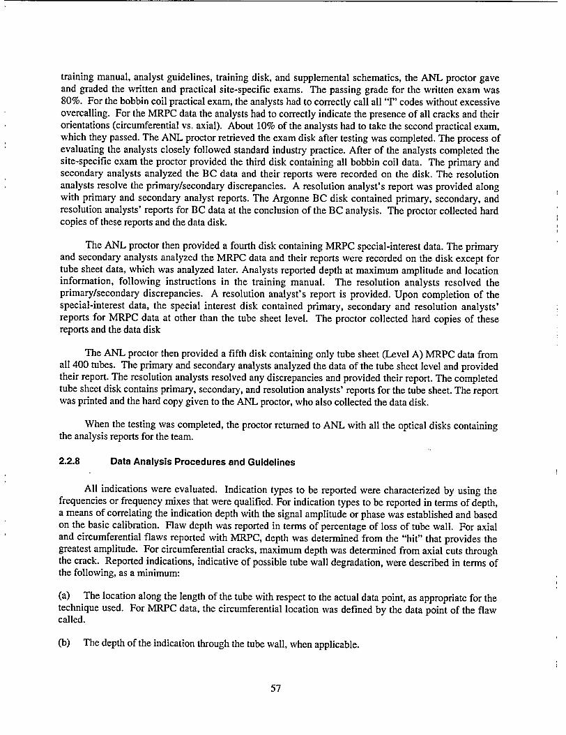
training manual, analyst guidelines, training disk, and supplemental schematics, the ANL proctor gave and graded the written and practical site-specific exams. The passing grade for the written exam was 80%. For the bobbin coil practical exam, the analysts had to correctly call all "I" codes without excessive overcalling. For the MRPC data the analysts had to correctly indicate the presence of all cracks and their orientations (circumferential vs. axial). About 10% of the analysts had to take the second practical exam, which they passed. The ANL proctor retrieved the exam disk after testing was completed. The process of evaluating the analysts closely followed standard industry practice. After of the analysts completed the site-specific exam the proctor provided the third disk containing all bobbin coil data. The primary and secondary analysts analyzed the BC data and their reports were recorded on the disk. The resolution analysts resolve the primary/secondary discrepancies. A resolution analyst's report was provided along with primary and secondary analyst reports. The Argonne BC disk contained primary, secondary, and resolution analysts' reports for BC data at the conclusion of the BC analysis. The proctor collected hard copies of these reports and the data disk.

The ANL proctor then provided a fourth disk containing MRPC special-interest data. The primary and secondary analysts analyzed the MRPC data and their reports were recorded on the disk except for tube sheet data, which was analyzed later. Analysts reported depth at maximum amplitude and location information, following instructions in the training manual. The resolution analysts resolved the primary/secondary discrepancies. A resolution analyst's report is provided. Upon completion of the special-interest data, the special interest disk contained primary, secondary and resolution analysts' reports for MRPC data at other than the tube sheet level. The proctor collected hard copies of these reports and the data disk

The ANL proctor then provided a fifth disk containing only tube sheet (Level A) MRPC data from all 400 tubes. The primary and secondary analysts analyzed the data of the tube sheet level and provided their report. The resolution analysts resolved any discrepancies and provided their report. The completed tube sheet disk contains primary, secondary, and resolution analysts' reports for the tube sheet. The report was printed and the hard copy given to the ANL proctor, who also collected the data disk.

When the testing was completed, the proctor returned to ANL with all the optical disks containing the analysis reports for the team.

2.2.8 Data Analysis Procedures and Guidelines

All indications were evaluated. Indication types to be reported were characterized by using the frequencies or frequency mixes that were qualified. For indication types to be reported in terms of depth, a means of correlating the indication depth with the signal amplitude or phase was established and based on the basic calibration. Flaw depth was reported in terms of percentage of loss of tube wall. For axial and circumferential flaws reported with MRPC, depth was determined from the "hit" that provides the greatest amplitude. For circumferential cracks, maximum depth was determined from axial cuts through the crack. Reported indications, indicative of possible tube wall degradation, were described in terms of the following, as a minimum:

(a) The location along the length of the tube with respect to the actual data point, as appropriate for the technique used. For MRPC data, the circumferential location was defined by the data point of the flaw called.

(b) The depth of the indication through the tube wall, when applicable.

57

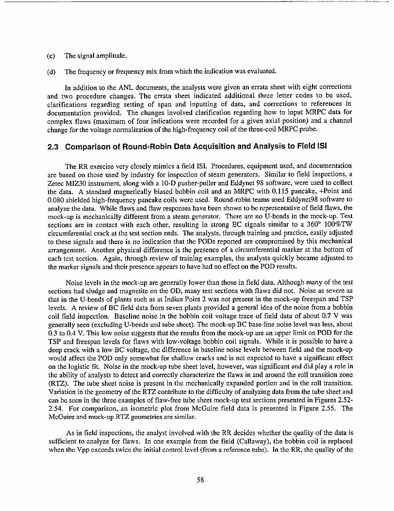
(c) The signal amplitude.

(d) The frequency or frequency mix from which the indication was evaluated.

In addition to the ANL documents, the analysts were given an errata sheet with eight corrections and two procedure changes. The errata sheet indicated additional three letter codes to be used, clarifications regarding setting of span and inputting of data, and corrections to references in documentation provided. The changes involved clarification regarding how to input MRPC data for complex flaws (maximum of four indications were recorded for a given axial position) and a channel change for the voltage normalization of the high-frequency coil of the three-coil MRPC probe.

2.3 Comparison of Round-Robin Data Acquisition and Analysis to Field ISI

The RR exercise very closely mimics a field ISI. Procedures, equipment used, and documentation are based on those used by industry for inspection of steam generators. Similar to field inspections, a Zetec MIZ30 instrument, along with a 10-D pusher-puller and Eddynet 98 software, were used to collect the data. A standard magnetically biased bobbin coil and an MRPC with 0.115 pancake, +Point and 0.080 shielded high-frequency pancake coils were used. Round-robin teams used Eddynet98 software to analyze the data. While flaws and flaw responses have been shown to be representative of field flaws, the mock-up is mechanically different from a steam generator. There are no U-bends in the mock-up. Test sections are in contact with each other, resulting in strong EC signals similar to a 3600 100%TW circumferential crack at the test section ends. The analysts, through training and practice, easily adjusted to these signals and there is no indication that the PODs reported are compromised by this mechanical arrangement. Another physical difference is the presence of a circumferential marker at the bottom of each test section. Again, through review of training examples, the analysts quickly became adjusted to the marker signals and their presence appears to have had no effect on the POD results.

Noise levels in the mock-up are generally lower than those in field data. Although many of the test sections had sludge and magnetite on the OD, many test sections with flaws did not. Noise as severe as that in the U-bends of plants such as at Indian Point 2 was not present in the mock-up freespan and TSP levels. A review of BC field data from seven plants provided a general idea of the noise from a bobbin coil field inspection. Baseline noise in the bobbin coil voltage trace of field data of about 0.7 V was generally seen (excluding U-bends and tube sheet). The mock-up BC base-line noise level was less, about 0.3 to 0.4 V. This low noise suggests that the results from the mock-up are an upper limit on POD for the TSP and freespan levels for flaws with low-voltage bobbin coil signals. While it is possible to have a deep crack with a low BC voltage, the difference in baseline noise levels between field and the mock-up would affect the POD only somewhat for shallow cracks and is not expected to have a significant effect on the logistic fit. Noise in the mock-up tube sheet level, however, was significant and did play a role in the ability of analysts to detect and correctly characterize the flaws in and around the roll transition zone (RTZ). The tube sheet noise is present in the mechanically expanded portion and in the roll transition. Variation in the geometry of the RTZ contribute to the difficulty of analyzing data from the tube sheet and can be seen in the three examples of flaw-free tube sheet mock-up test sections presented in Figures 2.522.54. For comparison, an isometric plot from McGuire field data is presented in Figure 2.55. The McGuire and mock-up RTZ geometries are similar.

As in field inspections, the analyst involved with the RR decides whether the quality of the data is sufficient to analyze for flaws. In one example from the field (Callaway), the bobbin coil is replaced when the Vpp exceeds twice the initial control level (from a reference tube). In the RR, the quality of the

58

Isometric plot of mock-up tube sheet level roll transition from data collected by rotating +Point coil at 300 kHz (example 1).

Isometric plot of mock-up tubesheet level roll transition from data collected by rotating +Point coil at 300 kHz (example 2).

59

- hlEC SGIIHCAL00015WVED W.39 24 DEC-01-18999 SG 11 R 6 C 6 1010 [MB)

1091

* 1847

Figure 2.52

Figure 2.53

"RPIZ6">1,HCALOOOI9YEOf 129:2 DFCO1-1999SG I tI C II W2 (Mal

P0 "\FY WV" ROT ftoi -n

NN

4.5k

9 .5o 6

to L.2

Isometric plot of mock-up tubesheet level roll transition from data collected by rotating +Point coil at 300 kHz (example 3).

Isometric plot of roll transition in tube sheet from McGuire steam generator

60

8C Pc •SolICALCiOISED 11 4108 DEC-O1-.1l09 S 11 R 12 C S 041 [MDT

ýAm ý,ff i• imA mall

cIIN

0.00

Figure 2.54

Figure 2.55

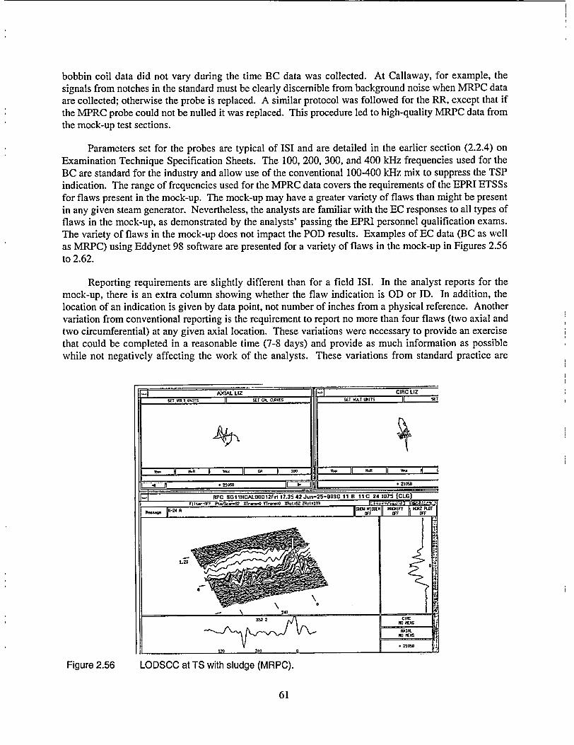
bobbin coil data did not vary during the time BC data was collected. At Callaway, for example, the signals from notches in the standard must be clearly discernible from background noise when MRPC data are collected; otherwise the probe is replaced. A similar protocol was followed for the RR, except that if the MPRC probe could not be nulled it was replaced. This procedure led to high-quality MRPC data from the mock-up test sections.

Parameters set for the probes are typical of ISI and are detailed in the earlier section (2.2.4) on Examination Technique Specification Sheets. The 100, 200, 300, and 400 kHz frequencies used for the BC are standard for the industry and allow use of the conventional 100-400 kHz mix to suppress the TSP indication. The range of frequencies used for the MPRC data covers the requirements of the EPRI ETSSs for flaws present in the mock-up. The mock-up may have a greater variety of flaws than might be present in any given steam generator. Nevertheless, the analysts are familiar with the EC responses to all types of flaws in the mock-up, as demonstrated by the analysts' passing the EPRI personnel qualification exams. The variety of flaws in the mock-up does not impact the POD results. Examples of EC data (BC as well as MRPC) using Eddynet 98 software are presented for a variety of flaws in the mock-up in Figures 2.56 to 2.62.

Reporting requirements are slightly different than for a field ISI. In the analyst reports for the mock-up, there is an extra column showing whether the flaw indication is OD or ID. In addition, the location of an indication is given by data point, not number of inches from a physical reference. Another variation from conventional reporting is the requirement to report no more than four flaws (two axial and two circumferential) at any given axial location. These variations were necessary to provide an exercise that could be completed in a reasonable time (7-8 days) and provide as much information as possible while not negatively affecting the work of the analysts. These variations from standard practice are

Figure 2.56

AXIAL LIZ CIRC LIZ

VOT UNITS SET CR. CUVES SET IAXT UNITS SOT

SVPP A ~ GA -105 VW~ ~ .

2105- .21058

FPC SGI1HCALCOO12Fri 17.35 42 Jun-25-BOSG 11 0 11 C 24 1075 [CLGI Fll IGASF Pt,/Sc...21 XT,- YfrVT 0.0.02250.

MeawI-24 A ISHU1 "IDE 1021FffTI PLOT

5 ;

- 2!240 3522 CIRC

1.221059

at h M

LODSCC at TS with sludge (MRPC).

61

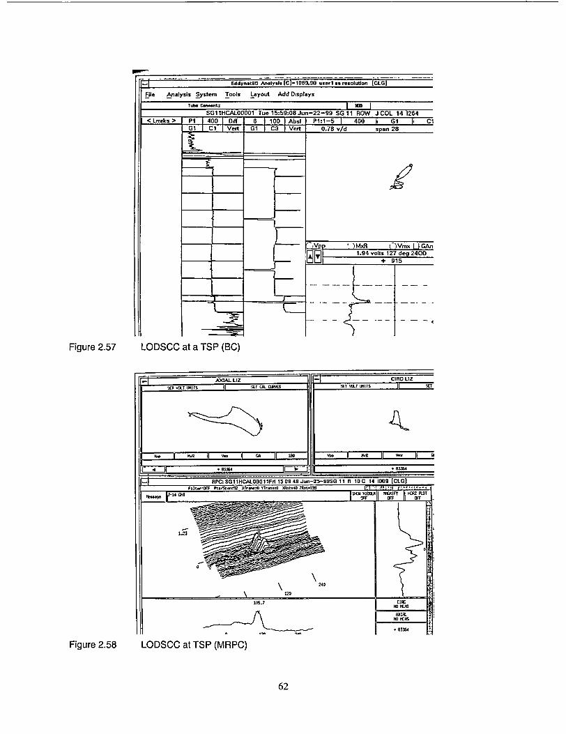
EddynetgB Analysls [C]-1189,90 userl as resolution [CLG]

File Analysis System Tools Layout Add Displays

Tub. Ceae-et:

SG11HCALO000I Tue 15:59:08 Jun-22-99 SG 11 ROW J COL 14 1264

< Lmrks > I P1 400 1 Dri 6 8 100 AbslI P10-5 400 I G C1

G1 I CI I VertI GI I C3 I Vert1 0.78v/d span 281* I - --

• )MxR i-)Vmx L[ GAn

1.94 volts 127 deg 240D + 915

Figure 2.57 LODSCC at a TSP (BC)

LODSCC at TSP (MRPC)

62

I

Figure 2.58

i E

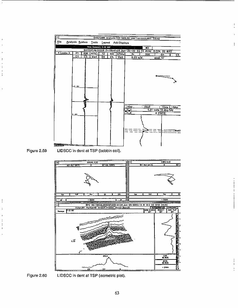
LIDSCC in dent at TSP (bobbin coil).

Figure 2.60 LIDSCC in dent at TSP (isometric plot).

63

Figure 2.59

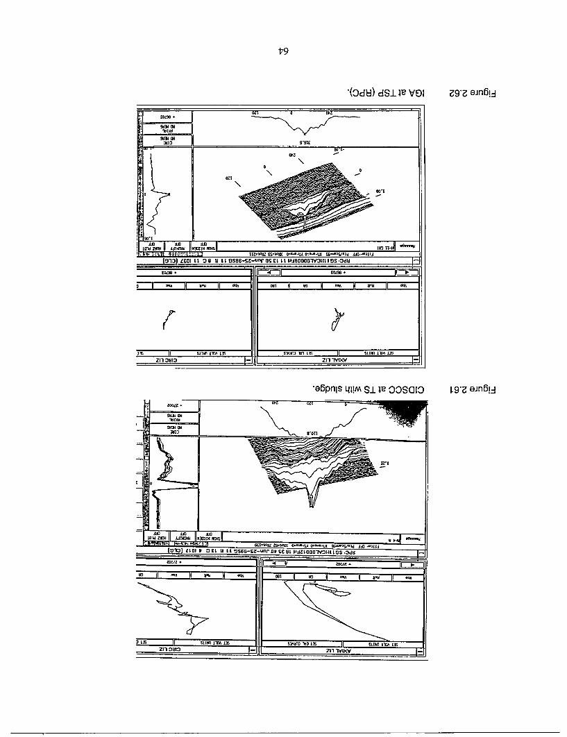
oz

ozi

0 903

90'T

INO T144 1 -1 W-VW S4-W 0--IIA W-IX t&--./-Id dA-1111

19-13) LEDI Lg 39 11 t I C)SSG-.SZ-Unr 8S C I L I PAGOODOW3R9 I DS -3dU

EWA IaM

a -A V.W 11 ddA OST W K -A VW

135 SAINI IIDA L35 s3MM 153 135 gliNn I-M Lis

Zil OU13 ýýj zil Tqlxv a Eýjl

t,9

,e6pnls ql!m Si ju OOS(]Io Lg-Z ein6ij

'(OdH) dS.L lu VOI Zq-Z ein6ij

carefully described in the training manual and analyst guidelines. The analysts made the adjustment to the mock-up reporting requirements quickly. A primary objective of the RR is to establish the POD for deep flaws. While some deep flaws may result in relatively low EC signal amplitude, the deep flaws generally have high signal amplitudes. As a result, although the voltage histogram for the mock-up flaws looks reasonable, there are more high-voltage signals than would be expected from a field inspection. A review of field data, such as from McGuire (a better than average plant), shows that while BC signals from TTS can be many volts in amplitude (i.e. >10 V), the signals from the TSP regions are primarily less than 3 V, with most less than 1 V in the 100-400 kHz mix channel. Stronger TSP flaw signals can be found in the mock-up because of the emphasis on deep flaws.

Analysis training and testing for the RR is comparable to that for a field ISI. For example, in a recent outage at the Union Electric Callaway Plant, a training class was presented on examples of Callaway's active degradation as well as potential degradations: ding and freespan OD cracking. This protocol is virtually the same as for the mock-up except that a formal class was not arranged. At Callaway, personnel performing the data analysis were required to successfully complete a site specific performance demonstration involving bobbin coil and MRPC data prior to performing any data analysis. The written exam covered design, data acquisition, and analysis. The practical exam covered in-situ tubes with calls based on expert opinion. Overcalls were allowed for up to 10% of all intersections. Passing required a correct call as to whether a crack is axial or circumferential. For rotating probe data, 100% on detection and orientation is required to pass the test. This protocol on testing is identical in every respect to that for the ANL mock-up.

2.4 Strategy for Evaluation of Results

2.4.1 General Principles

POD has been determined for the flaws in the mock-up as a function of flaw type and flaw location (i.e., freespan, TSP, and tubesheet). The PODs have been plotted against maximum depth, mp, average depth, and, for the case of circumferential cracking, area. Logistic fits have been calculated and include errors in depth sizing and false call rates. Upper and lower 95% confidence limits are included in the logistic fit curves. An analyst is given credit for detecting a flaw if the call is an "I" code (e.g., NQI, DNI, DTI for BC calls, MAI, SAI, SCI, MCI, and MMI for MRPC calls) and the location is within 25 mm of the ends of the flaw.

2.4.2 Tolerance for Errors in Location

The location error allowed for calls made from bobbin coil data is 25 mm from either end of the flaw along the tube axis. This allowed error converts to 30 data points for bobbin coil data. For MRPC data the error allowed in the axial direction is also 25 mm from the ends of the flaw along the tube axis. This allowed error converts to 3000 data points for the MRPC data.

2.4.3 Handling of False Calls

Analysts' reports were used to determine the false call rate. The rate was determined from a review of randomly selected flaw-free test sections in the mock-up and the number of "I' codes called in those test sections. An "I" code call (NQI, DTI, DNI) indicates that a flaw-indication was present in the section even though no flaw was present. A total of 522 test sections were analyzed. No known stress corrosion cracks (SCC) were in any of the test sections. With 11 teams, there were 5742 chances to make a false

65

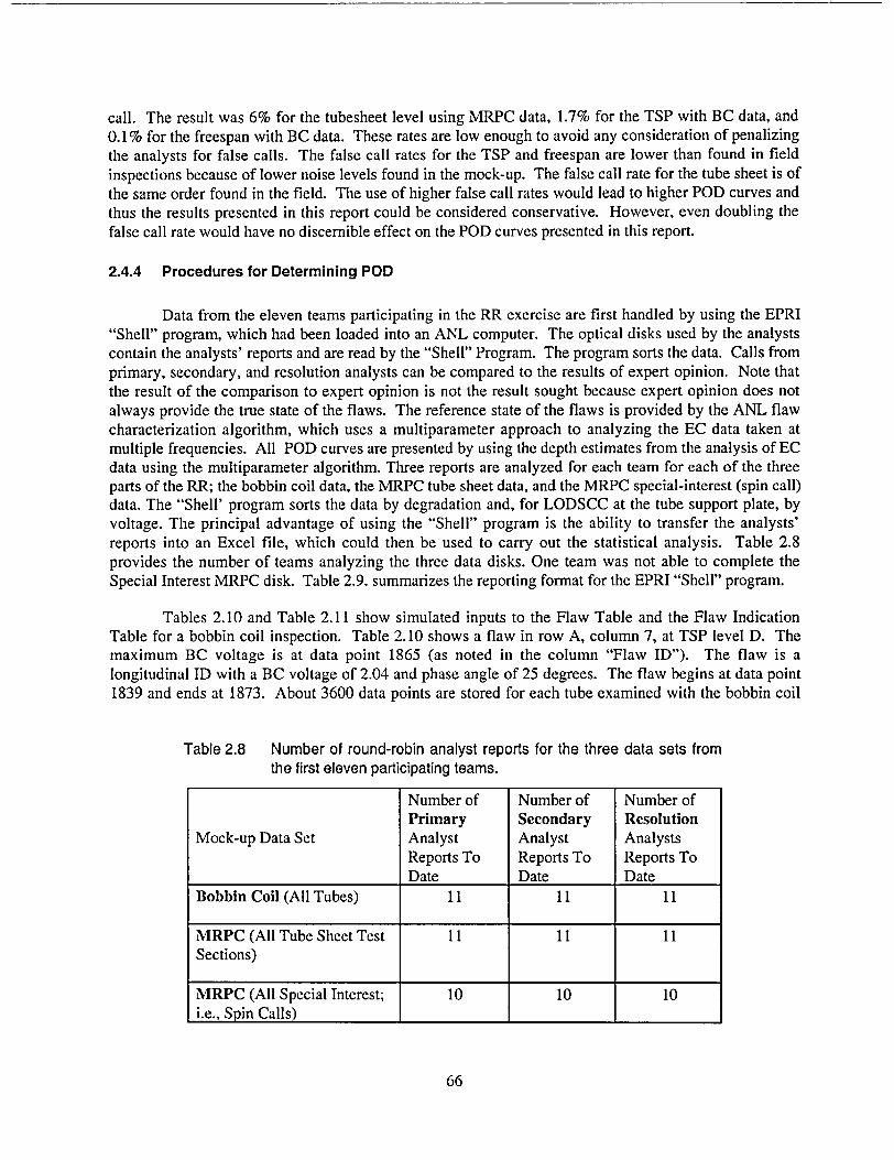
call. The result was 6% for the tubesheet level using MRPC data, 1.7% for the TSP with BC data, and 0.1% for the freespan with BC data. These rates are low enough to avoid any consideration of penalizing the analysts for false calls. The false call rates for the TSP and freespan are lower than found in field inspections because of lower noise levels found in the mock-up. The false call rate for the tube sheet is of the same order found in the field. The use of higher false call rates would lead to higher POD curves and thus the results presented in this report could be considered conservative. However, even doubling the false call rate would have no discernible effect on the POD curves presented in this report.

2.4.4 Procedures for Determining POD

Data from the eleven teams participating in the RR exercise are first handled by using the EPRI "Shell" program, which had been loaded into an ANL computer. The optical disks used by the analysts contain the analysts' reports and are read by the "Shell" Program. The program sorts the data. Calls from primary, secondary, and resolution analysts can be compared to the results of expert opinion. Note that the result of the comparison to expert opinion is not the result sought because expert opinion does not always provide the true state of the flaws. The reference state of the flaws is provided by the ANL flaw characterization algorithm, which uses a multiparameter approach to analyzing the EC data taken at multiple frequencies. All POD curves are presented by using the depth estimates from the analysis of EC data using the multiparameter algorithm. Three reports are analyzed for each team for each of the three parts of the RR; the bobbin coil data, the MRPC tube sheet data, and the MRPC special-interest (spin call) data. The "Shell' program sorts the data by degradation and, for LODSCC at the tube support plate, by voltage. The principal advantage of using the "Shell" program is the ability to transfer the analysts' reports into an Excel file, which could then be used to carry out the statistical analysis. Table 2.8 provides the number of teams analyzing the three data disks. One team was not able to complete the Special Interest MRPC disk. Table 2.9. summarizes the reporting format for the EPRI "Shell" program.

Tables 2.10 and Table 2.11 show simulated inputs to the Flaw Table and the Flaw Indication Table for a bobbin coil inspection. Table 2.10 shows a flaw in row A, column 7, at TSP level D. The maximum BC voltage is at data point 1865 (as noted in the column "Flaw ID"). The flaw is a longitudinal ID with a BC voltage of 2.04 and phase angle of 25 degrees. The flaw begins at data point 1839 and ends at 1873. About 3600 data points are stored for each tube examined with the bobbin coil

Table 2.8 Number of round-robin analyst reports for the three data sets from the first eleven participating teams.

Number of Number of Number of Primary Secondary Resolution

Mock-up Data Set Analyst Analyst Analysts Reports To Reports To Reports To Date Date Date

Bobbin Coil (All Tubes) 11 11 11

MRPC (All Tube Sheet Test 11 11 11 Sections)

MRPC (All Special Interest; 10 10 10 i.e., Spin Calls) I I I-

66

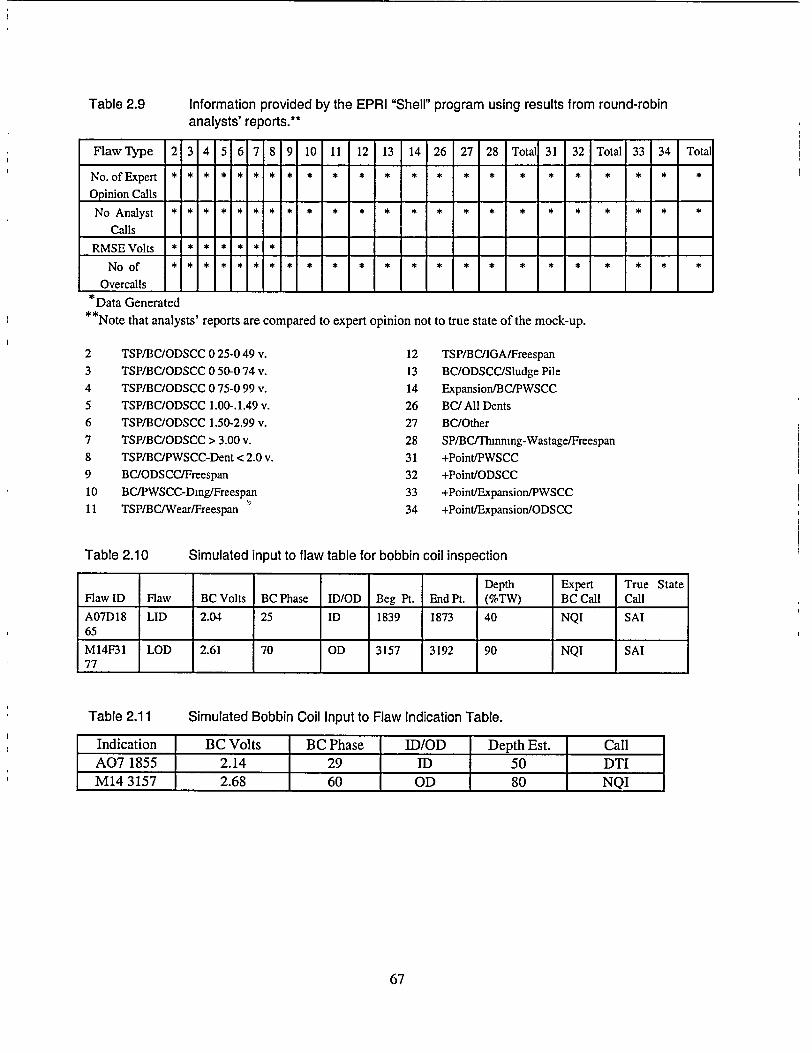
Table 2.9 Information provided by the EPRI "Shell" program using results from round-robin analysts' reports.**

FlawType 2 3 4 5 6 7 8 9 10 11 12 13 14 26 27 28 Total 31 32 Total 33 34 Tot

No. of Expert * * * * * * * * * * * * * * * * * * * * * * *

Opinion Calls

No Analyst * * * * * * * * * * * * * * * * * * * * * * *

Calls

RMSEVolts * * * * * * *

No of * * * * * * * * * * * * * * * * * * * * *

Overcalls * Data Generated

**Note that analysts' reports are compared to expert opinion not to true state of the mock-up.

TSP/BC/ODSCC 0 25-0 49 v. TSP/BC/ODSCC 0 50-0 74 v.

TSP/BC/ODSCC 0 75-0 99 v.

TSP/BC/ODSCC 1.00-.1.49 v.

TSP/BC/ODSCC 1.50-2.99 v.

TSP/BC/ODSCC > 3.00 v.

TSP/BC/PWSCC-Dent < 2.0 v.

BC/ODSCC/Freespan

BC/PWSCC-Ding/Freespan

TSP/BC/Wear/Freespan

Table 2.10

Table 2.11

12 TSP/BC/IGA/Freespan

13 BC/ODSCC/Sludge Pile

14 Expansion/BC/PWSCC

26 BC/All Dents 27 BC/Other

28 SP/BCilunning-Wastage/Freespan

31 +Point/PWSCC

32 +Point/ODSCC

33 +Point/Expansion/PWSCC

34 +Point/Expansion/ODSCC

Simulated input to flaw table for bobbin coil inspection

Simulated Bobbin Coil Input to Flaw Indication Table.

67

2

3

4

5

6

7

8

9

10

11

Depth Expert True State Flaw ID Flaw BC Volts BC Phase ID/OD Beg Pt. End Pt. (%TW) BC Call Call

A07D18 LID 2.04 25 ID 1839 1873 40 NQI SAI 65

M14F31 LOD 2.61 70 OD 3157 3192 90 NQI SAI 77

Indication BC Volts BC Phase ID/OD Depth Est. Call A07 1855 2.14 29 ID 50 DTI M14 3157 2.68 60 OD 80 NQI

(nine test sections). Table 2.10 shows a depth estimated to be 40%TW. This depth is determined by application of a multiparameter algorithm to MRPC data for the flaw. An "I" code triggers an inspection with an MRPC. The reference-state three-letter code is SAL, single axial indication. A second example is also provided. The second flaw, a longitudinal ODSCC, is at row M, column 14, and at freespan level F. The result for the bobbin coil inspection is shown in Table 2.11. An indication was found in row A, column 7, at data point 1855, close to the correct flaw location. The ID/OD call is correct and an "I" code is also called, although in this case it is DTI (distorted TSP indication). The DTI call also requires MRPC data to be acquired. The second indication would also be graded as a correct call. Indication tables are generated for both bobbin coil and MRPC data and compared with the Flaw Indication Table, which contains all information needed to estimate POD.

2.4.4.1 Converting SSPD Result to Text Files and Excel Files

The Eddynet software provides a series of files that contain the reports of results from each analyst who participated in the RR. These data are saved under an Eddynet environment and are identified by extensions that refer to primary, secondary, and resolution analysts' reports. These files were then read by a text editor and converted into a format useable for off-line manipulation. The text files were then imported into Excel. Excel macros were written to sort the results and carry out the grading.

2.5 Statistical Analysis

2.5.1 Determination of Logistic Fits

To obtain an analytical form for the probability of detection curve, we assume that the probability of detection as a function of depth can be expressed as a linear logistic function of x:

1 p(x) + ea+bx ' (3)

or

p(x) = logistic(a + bx)

where a and b are parameters that will be determined by comparison with the observed results. Other forms for the POD curve can be chosen, but the linear logistic curve has been widely used for this purpose, and is widely used in other fields to describe binomial responses (detected or not detected) [4].

The Method of Maximum Likelihood [5] is widely used to estimate statistical parameters such as a and b. For quantities that are normally distributed, it can be shown to be equivalent to the familiar method of least squares [5-6]. It is more generally applicable, however, and can be applied to events such as detection of cracks that are not normally distributed.

If p(x) is the probability that a crack of depth x will be detected by an inspection team, the probability that the crack will not be detected is 1-p(x). The probability that n out of N teams of inspectors will detect a crack of depth x is

nN) pn (i- p)N-n ,(4)

68

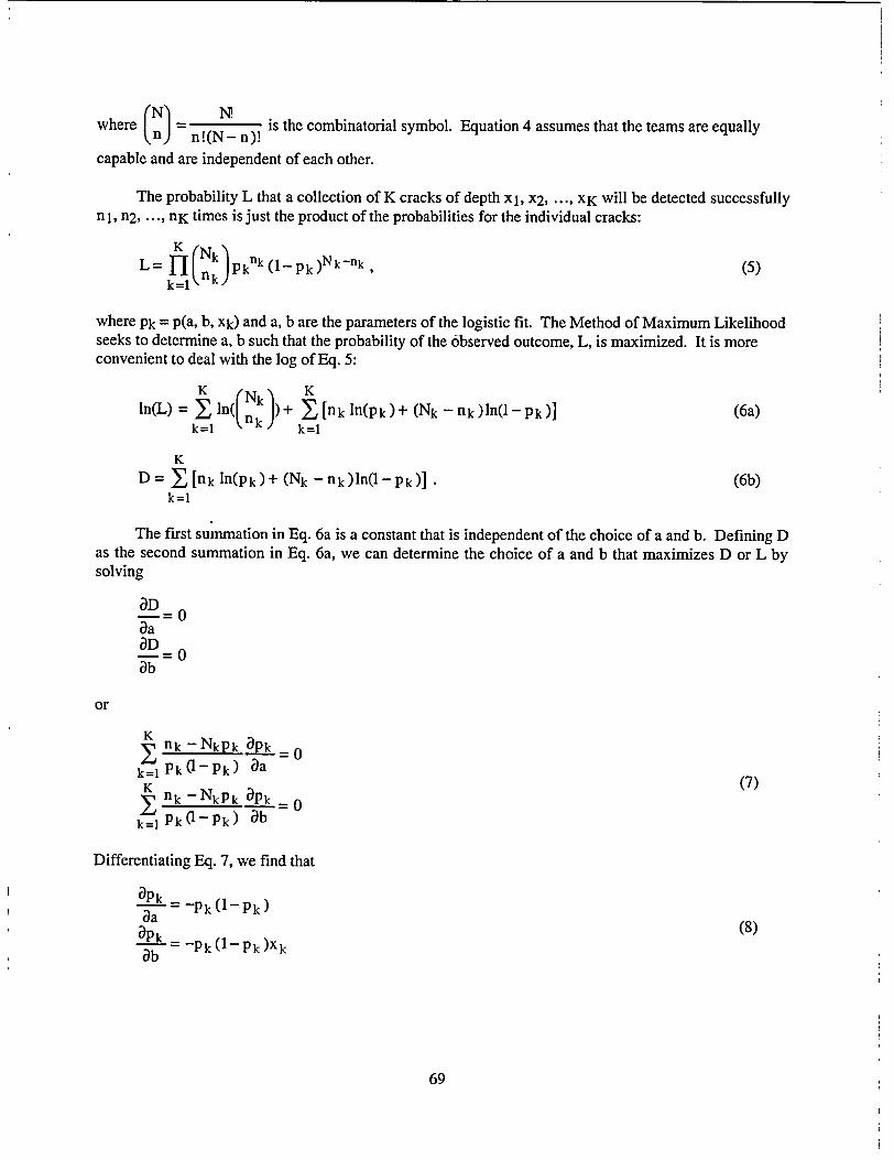
nwhne (NN is the combinatorial symbol. Equation 4 assumes that the teams are equally where ) n !(N - n)!

capable and are independent of each other.

The probability L that a collection of K cracks of depth x1, X2, .... X(K will be detected successfully n 1, n2 .... nK times is just the product of the probabilities for the individual cracks:

L= r(Nkiipknk (1pk)N k k(5) L= ,1n Pk O-k 5

where Pk = p(a, b, xk) and a, b are the parameters of the logistic fit. The Method of Maximum Likelihood seeks to determine a, b such that the probability of the observed outcome, L, is maximized. It is more convenient to deal with the log of Eq. 5:

K (Nk K ln(L) = Z ,n(Ink )+ F [nk ln(pk) + (Nk - nk)ln(1 - Pk)] (6a)

k=1 k=1

K D I[nk ln(pk) + (Nk - nk )ln(1 - pk)] • (6b)

k=1

The first summation in Eq. 6a is a constant that is independent of the choice of a and b. Defining D as the second summation in Eq. 6a, we can determine the choice of a and b that maximizes D or L by solving

aD -•=0

aa -=0 ab

or

K nk -Nkpk aPk=0

k=1 Pk(1-Pk) aa =0 K nk -NkPk aPk =0

k=1 Pk-G Pk) ab

Differentiating Eq. 7, we find that

aP- = -Pk G- Pk) aa (8)

af' = -Pk(1-Pk)xk ab

69

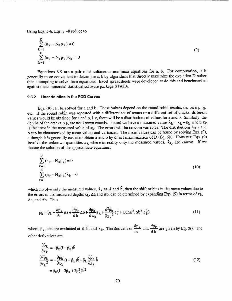
Using Eqs. 5-6, Eqs. 7 -8 reduce to

K

S(nk -NkPk)= 0 k =1 (9) K I (nk - NkPk)Xk = 0 k=1

Equations 8-9 are a pair of simultaneous nonlinear equations for a, b. For computation, it is

generally more convenient to determine a, b by algorithms that directly maximize the expiation D rather than attempting to solve these equations. Excel spreadsheets were developed to do this and benchmarked against the commercial statistical software package STATA.

2.5.2 Uncertainties in the POD Curves

Eqs. (9) can be solved for a and b. These values depend on the round robin results, i.e, on nI, n2, etc. If the round robin was repeated with a different set of teams or a different set of cracks, different values would be obtained for a and b, i. e, there will be a distributions of values for a and b. Similarly, the depths of the cracks, xk, are not known exactly, instead we have a measured value Xk = Xk + Ek where Ek is the error in the measured value of xk. The errors will be random variables. The distributions for a and b can be characterized by mean values and variances. The mean values can be found by solving Eqs. (9), although it is generally easier to obtain a and b by direct maximization of D (Eq. 6b). However, Eqs. (9) involve the unknown quantities xk where in reality only the measured values, xk, are known. If we denote the solution of the approximate equations,

K E (nk - NkAk)=0

k=1 (10) K

E (nk - NkJk):k = 0

k=1

which involve only the measured values, Xk as a and b, then the shift or bias in the mean values due to

the errors in the measured depths xk, Aa and Ab, can be dtermined by expanding Eqs. (9) in terms of Ek, Aa, and Ab. Thus

kpk- Aa+k ak E21 2(11)3

Pk =Pk + •- Aa + Ab+ - Ek + 2 2+ O(Aa2 ,Ab2 ,) ( axk axk

where Pk, etc. are evaluated at i, b, and Xk. The derivatives p and L are given by Eq. (8). The aa aTb

other derivatives are

ahk = _Pk(l -Pk)b axk

a 2 =aPk( 1 -k)b+k Pb (12)

axk axk aXk

Pk(1- 3pk +2p3)2

70

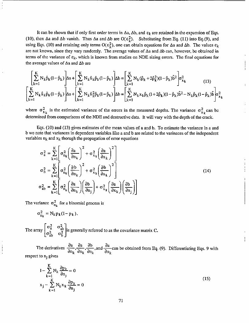
It can be shown that if only first order terms in Aa, Ab, and Ek are retained in the expansion of Eqs. (10), then Aa and Ab vanish. Thus Aa and Ab are O(2). Substituting from Eq. (11) into Eq.(9), and using Eqs. (10) and retaining only terms O(e2), one can obtain equations for Aa and Ab. The values Ek are not known, since they vary randomly. The average values of Aa and Ab can, however, be obtained in terms of the variance of Ek, which is known from studies on NDE sizing errors. The final equations for the average values of Aa and Ab are

L=NkPk (I1- P0) Aa + Ek =Nk~kPk(1 - Pk) Ab = L•INk(Pk k 2)1- Pk l2CT~k (13)

[ NkikPk(1-Pk) Aa+[ Nki kk(1-Pk) Ab = Nkxk~k(1+2Pk)(1-k) 2 - Nk~k(1- k X IkIl k=1 1 . where 132 is the estimated variance of the errors in the measured depths. The variance C;2 can be

Xk Xk determined from comparisons of the NDE and destructive data. It will vary with the depth of the crack.

Eqs. (10) and (13) gives estimates of the mean values of a and b. To estimate the variance in a and b we note that variances in dependent variables like a and b are related to the varinaces of the independent variables nk and Xk thorugh the propagation of error equations

aY [,2 ( 'a +U2a

a k= Y- k ank Xk aXk

nk=

ar 2 K [( 2 ( +ba2 CF 2] (14)

k=1 E nk a xk ) -kan d -X a bXke axijq

k=1 n

The variance a2 for a binomial process is

nkk

x2 -=NkPk(--Pk).

The array a 2 a ~is generally referred to as the covariance matrix C. L ab abJ

The derivatives -,-,-,aband -acan be obtained from Eq. (9). Differentiating Eqs. 9 with ank' xkv 9f x

respect to nj gives

I- Eka k=1 J (15) K aPk= xj-ENkxk-ank=1

71

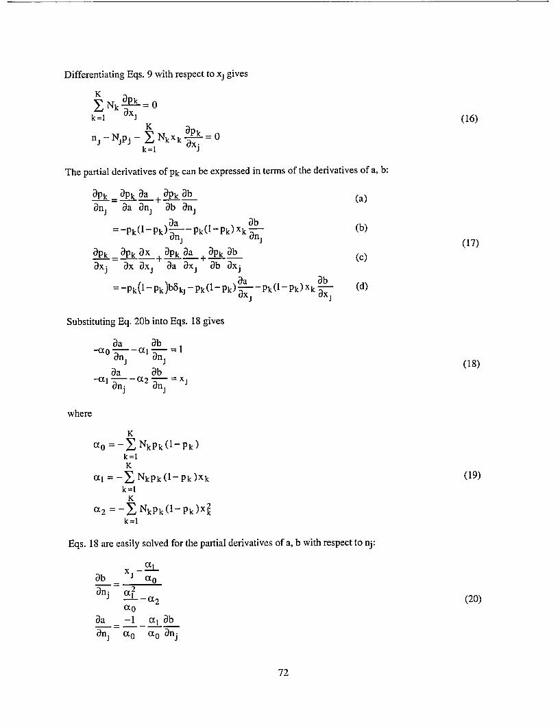
Differentiating Eqs. 9 with respect to xj gives

k=l (16) K aPk

nj-Njpj- ENkxk -o

k=1 j

The partial derivatives of Pk can be expressed in terms of the derivatives of a, b:

aPk = aPk aa +-aPk ab (a)

anl aa aan1 b ani

-Pk(Pk)Pk(IPk) k (b) ani -ani(17)

aPk _ aPk ax + aPk aa + aPk ab (c)

a x ax aa axa ab ax(

-Pk(1-pk)bakj-Pk(1-Pk)• -Pk( Pk)Xk a (d)

Substituting Eq. 20b into Eqs. 18 gives

aa ab -'•0 -51 =1 an ab (18)

--X'Inaa--CC2"an = x)

where

K a0 =-ENkPk(1--Pk)

k=1 K

cl = -E NkPk (l-pk)Xk (19) k=1

K CC2 =-XNkPk(1-pk)xk

k=1

Eqs. 18 are easily solved for the partial derivatives of a, b with respect to nj:

50`

an- aX2

j -_ 2 (20) 5 0

aa -1 cc ab ani ac0 50 anj

72

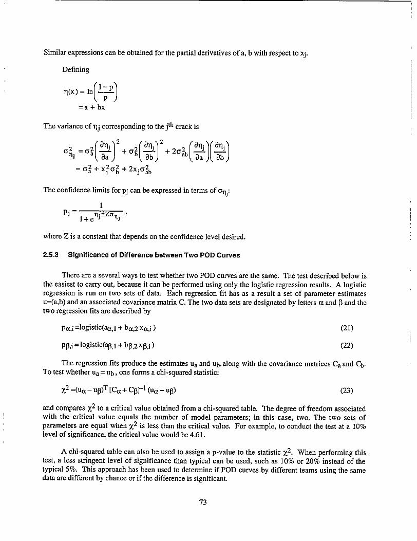
Similar expressions can be obtained for the partial derivatives of a, b with respect to Xj.

Defining

Tj(x) =-I .

=a + bx

The variance of ilj corresponding to the jth crack is

0T2 -,2 ( ii 2+ y2( Il 2 + 2C2 'i'rm" j Oa b La (> 'Ilit g)L ~ ~ aa) b- 7 ab aa ,.ab)

: o2 + x2<y2 + 2xjo 2 a Xj b + Jab

The confidence limits for pj can be expressed in terms of ollj

1 pj = 1+e erjZoI

'

where Z is a constant that depends on the confidence level desired.

2.5.3 Significance of Difference between Two POD Curves

There are a several ways to test whether two POD curves are the same. The test described below is the easiest to carry out, because it can be performed using only the logistic regression results. A logistic regression is run on two sets of data. Each regression fit has as a result a set of parameter estimates u=(a,b) and an associated covariance matrix C. The two data sets are designated by letters (x and f0 and the two regression fits are described by

Pax,i =logistic(ajl + ba,2 xaj) (21)

pp = logistic(ap3,1 + b0,2 x3,i ) (22)

The regression fits produce the estimates ua and ub, along with the covariance matrices Ca and Cb. To test whether ua = ub, one forms a chi-squared statistic:

i2 =(ua - uO)T [Ca + CO3-' 1 (ua - u1) (23)

and compares x2 to a critical value obtained from a chi-squared table. The degree of freedom associated with the critical value equals the number of model parameters; in this case, two. The two sets of parameters are equal when X2 is less than the critical value. For example, to conduct the test at a 10% level of significance, the critical value would be 4.61.

A chi-squared table can also be used to assigna p-value to the statistic X2. When performing this test, a less stringent level of significance than typical can be used, such as 10% or 20% instead of the typical 5%. This approach has been used to determine if POD curves by different teams using the same data are different by chance or if the difference is significant.

73

2.6 Results of Analysis Round-Robin

The lack of reliability in estimating the maximum depth of an SCC with either voltage or phase

angle from bobbin coil data, a well known problem in field inspections, can be illustrated for the mock-up

with results from the RR. Figure 2.63 shows the relationship of BC voltage and maximum depth

(determined from the multiparameter algorithm) for LODSCC and LIDSCC. While very high voltages

(>10 V) indicate deep flaws (>80%TW), lower amplitudes do not correlate with depth. The results for

TSP and freespan are similar. Figure 2.64 shows the relationship of BC phase angle to maximum depth

of LODSCC at the TSP. For LODSCC, ideally the phase angle should increase monotonically from 400

as the depth increases. The scatter indicates the difficulty in using BC phase angle to estimate depth.

Figure 2.65 shows a similar result for LIDSCC at the TSP. For LIDSCC, the phase should increase from 0 to 40' as the depth increases from 0 to 100%TW.

2.6.1 POD Logistic Fits with 95% Lower Confidence Bounds

An analysis of bobbin coil voltages reported for LODSCC at tube support plates by teams analyzing

the mock-up data has been carried out. In most cases, voltage variations identified by the teams were fairly small. For each LODSCC, an average BC voltage and a corresponding standard deviation were

computed. The cumulative distribution of the normalized standard deviations (i.e., the standard deviation divided by the corresponding value of the average voltage) can be fit well by a Weibull distribution (the RMS difference between the observed distribution and the Weibull fit is <0.03). The fitted distribution is shown in Figure 2.66. For almost 90% of the indications, the normalized standard deviation in the

reported voltages is < 0.15. This result is consistent with Generic letter 95-05 which assumes a 15 percent cutoff for the voltage response variability distribution is acceptable. The indications with larger variations are not associated with particularly high or low voltages (i.e., approximately half the signals with standard deviations of >0.1 have voltages of >2), but rather are associated with the complexity of the signal and the difficulty in identifying the peak voltage.

2.6.1.1 Bobbin Coil Results

The reference table shows the flaw parameters, max depth, mp, average depth, and for circumferential cracks the crack area and the observed POD. The flaw characterization parameters were determined from the profiles generated by the multiparameter algorithm. The results reported here are derived from the bobbin coil reports of resolution analysts from the eleven teams participating in the RR. Figures are shown for tube support plate and freespan flaws. Analysts are given credit for calling a flaw if their reported flaw location is within 25 mm (1 in.) of the ends of the flaw. The analyst's estimate of depth was not a factor in calculating POD.

Figures 2.67 shows the maximum likelihood logistic fit for POD for LODSCC and LIDSCC at the TSP as a function of maximum depth (as determined from the multiparameter algorithm). The NDE uncertainty in depth is included in the one-sided 95% lower confidence limit (OSL). In general, the curves have a reasonable shape, providing plausible PODs. As expected, the POD for ID cracks is higher than for OD cracks (99% with 98%OSL at 60%TW vs. 75% with 65%OSL at 60% TW). Figure 2.68 shows raw data and the logistic fit curve for the BC POD for one of the RR teams. As can be seen, the probability of a hit is very high for the deepest flaws, which are dominant in this set of cracks.

74

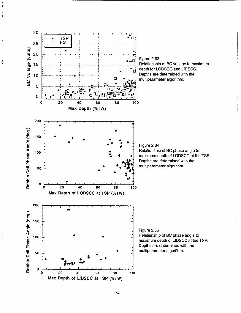
s0. TSP

25 o .FS .........................

"-6 20

0• 10

0 5 a, 5

0 20 40 60

Max Depth (%TW)

200

150

100

50

0

200

150

100

50

0

0 20 40 60 80

Max Depth of LODSCC at TSP (%TW)

0 20 40

Max Depth of LIDSCC60 at TSP

0 • Figure 2.63 .......... Relationship of BC voltage to maximum * • n n depth for LODSCC and LIDSCC. ..................... Depths are determined with the

g.. . multiparameter algorithm.

80 100

Figure 2.64 Relationship of BC phase angle to maximum depth of LODSCC at the TSP. Depths are determined with the multiparameter algorithm.

100

80 (%TW)

Figure 2.65 Relationship of BC phase angle to maximum depth of LIDSCC at the TSP. Depths are determined with the multiparameter algorithm.

100

75

.4

S---- - -- - - . . .. . ...- - - i -- -- . .. ........... .

--- .-- - - - - -.......... . .............. ... .... - - -------

; 0S _..,..,;.,... , ... , . o.t°i-a- . ,r

0

C 1-:

tM C

,o cc

02

(3

.0 0

~0 C

IC

0

0 M3

,I.

v.

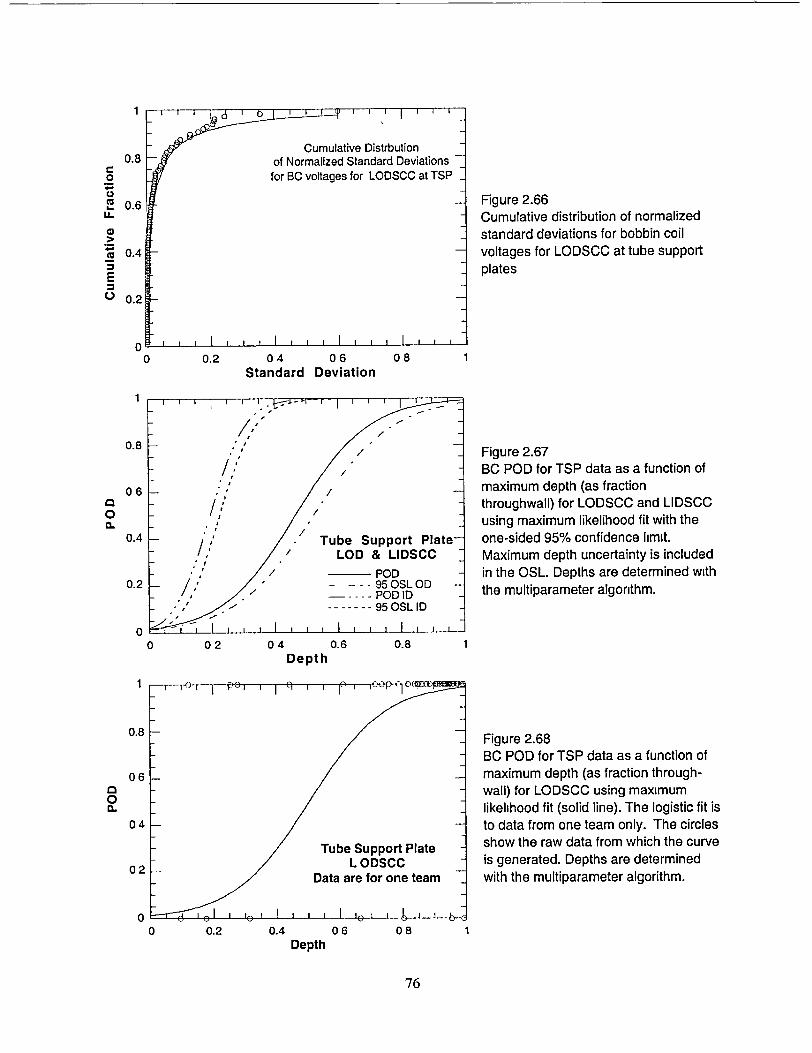
0.8

.0 for BC voltages for LODSCC at TSP

0.6 Figure 2.66 "U. Cumulative distribution of normalized

standard deviations for bobbin coil

.! 0.4 voltages for LODSCC at tube support E plates

o 0.2

o F I I I I I I I , 1I

0 0.2 04 06 08 1

Standard Deviation

0.8 /- Figure 2.67

, / BC POD for TSP data as a function of

0 6 / maximum depth (as fraction O /, throughwall) for LODSCC and LIDSCC

I' using maximum likelihood fit with the 0.4 . Tube Support Plate- one-sided 95% confidence limit.

/ / LOD & LIDSCC Maximum depth uncertainty is included

/ POD in the OSL. Depths are determined with 0.2 / ' - .... 95OSL OD 02 ---.. POD ID the multipararneter algorithm.

------- 95OSLID

0 0 02 04 0.6 0.8 1

Depth

1 I P E) i I I

0.8 Figure 2.68

BC POD for TSP data as a function of

06 maximum depth (as fraction throughO wall) for LODSCC using maximum 0 I0 likelihood fit (solid line). The logistic fit is

04 to data from one team only. The circles

Tube Support Plate show the raw data from which the curve

L ODSCC _ is generated. Depths are determined 02 Data are for one team with the multiparameter algorithm.

0 0 0.2 0.4 06 08 1

Depth

76

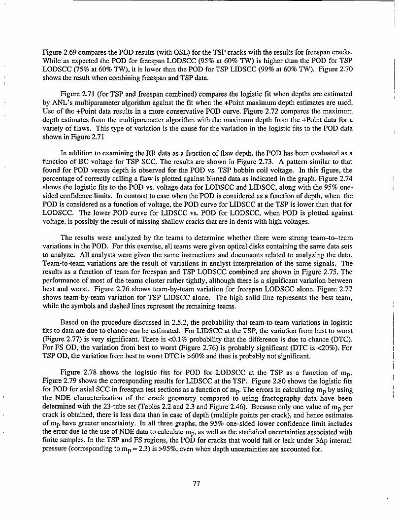
Figure 2.69 compares the POD results (with OSL) for the TSP cracks with the results for freespan cracks. While as expected the POD for freespan LODSCC (95% at 60% TW) is higher than the POD for TSP LODSCC (75% at 60% TW), it is lower than the POD for TSP LIDSCC (99% at 60% TW). Figure 2.70 shows the result when combining freespan and TSP data.

Figure 2.71 (for TSP and freespan combined) compares the logistic fit when depths are estimated by ANL's multiparameter algorithm against the fit when the +Point maximum depth estimates are used. Use of the +Point data results in a more conservative POD curve. Figure 2.72 compares the maximum depth estimates from the multiparameter algorithm with the maximum depth from the +Point data for a variety of flaws. This type of variation is the cause for the variation in the logistic fits to the POD data shown in Figure 2.71

In addition to examining the RR data as a function of flaw depth, the POD has been evaluated as a function of BC voltage for TSP SCC. The results are shown in Figure 2.73. A pattern similar to that found for POD versus depth is observed for the POD vs. TSP bobbin coil voltage. In this figure, the percentage of correctly calling a flaw is plotted against binned data as indicated in the graph. Figure 2.74 shows the logistic fits to the POD vs. voltage data for LODSCC and LIDSCC, along with the 95% onesided confidence limits. In contrast to case when the POD is considered as a function of depth, when the POD is considered as a function of voltage, the POD curve for LIDSCC at the TSP is lower than that for LODSCC. The lower POD curve for LIDSCC vs. POD for LODSCC, when POD is plotted against voltage, is possibly the result of missing shallow cracks that are in dents with high voltages.

The results were analyzed by the teams to determine whether there were strong team-to-team variations in the POD. For this exercise, all teams were given optical disks containing the same data sets to analyze. All analysts were given the same instructions and documents related to analyzing the data. Team-to-team variations are the result of variations in analyst interpretation of the same signals. The results as a function of team for freespan and TSP LODSCC combined are shown in Figure 2.75. The performance of most of the teams cluster rather tightly, although there is a significant variation between best and worst. Figure 2.76 shows team-by-team variation for freespan LODSCC alone. Figure 2.77 shows team-by-team variation for TSP LIDSCC alone. The high solid line represents the best team, while the symbols and dashed lines represent the remaining teams.

Based on the procedure discussed in 2.5.2, the probability that team-to-team variations in logistic fits to data are due to chance can be estimated. For LIDSCC at the TSP, the variation from best to worst (Figure 2.77) is very significant. There is <0.1% probability that the difference is due to chance (DTC). For FS OD, the variation from best to worst (Figure 2.76) is probably significant (DTC is <20%). For TSP OD, the variation from best to worst DTC is >60% and thus is probably not significant.

Figure 2.78 shows the logistic fits for POD for LODSCC at the TSP as a function of mp. Figure 2.79 shows the corresponding results for LIDSCC at the TSP. Figure 2.80 shows the logistic fits for POD for axial SCC in freespan test sections as a function of mp. The errors in calculating mp by using the NDE characterization of the crack geometry compared to using fractography data have been determined with the 23-tube set (Tables 2.2 and 2.3 and Figure 2.46). Because only one value of mp per crack is obtained, there is less data than in case of depth (multiple points per crack), and hence estimates of mp have greater uncertainty. In all three graphs, the 95% one-sided lower confidence limit includes the error due to the use of NDE data to calculate mp, as well as the statistical uncertainties associated with finite samples. In the TSP and FS regions, the POD for cracks that would fail or leak under 3Ap internal pressure (corresponding to mp = 2.3) is >95%, even when depth uncertainties are accounted for.

77

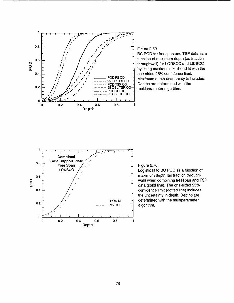
1

0.8 - ';, , 0.8"-Figure 2.69 /; 'BC POD for freespan and TSP data as a

0.6 * function of maximum depth (as fraction o.. throughwall) for LODSCC and LIDSCC a. / : by using maximum likelihood fit with the

0.4 - one-sided 95% confidence limit. ,i / ~POD FS OD Maximum depth uncertainty is included.

- .... 95OSLFSOD 0.2 - " - - POD TSP OD Depths are determined with the

0.2 ----- 95 OSL TSP OD PD- TSP D - multiparameter algorithm.

• •. . -" 95OSLTSPID

0 0.2 0.4 0.6 08 1 Depth

Combined 0 Tube Support Plate /

Free Span / Figure 2.70 LODSCC , Logistic fit to BC POD as a function of

0.6/ maximum depth (as fraction throughO wall) when combining freespan and TSP 0.

o•. data (solid line). The one-sided 95%

04 confidence limit (dotted line) includes the uncertainty in depth. Depths are

/ POD IML determined with the multiparameter 02 - 95 OSL algorithm.

0/

o 02I 0 I 0 1 0 0 2 0 4 0.6 0.81

Depth

78

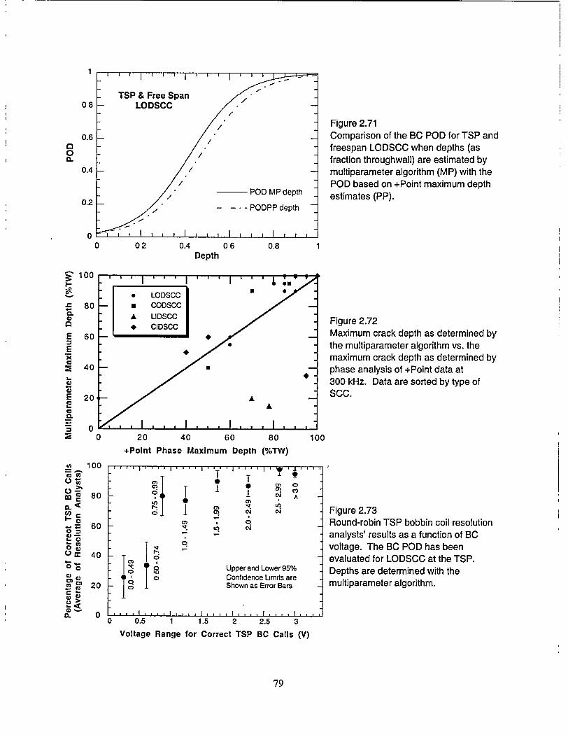
0 02 0.4 06 0.8 Depth

08

0.6

0.4

0.2

0

0 20 40 60 80 100

+Point Phase Maximum Depth (%TW)

0 I I

'1; C,. 0 C,.

cliA

C)

G!|' ' 1 '

0T

C;

C; on

6

Upper and Lower 95% Confidence Limits are Shown as Error Bars

0 0.5 1 1.5 2 2.5 3

Voltage Range for Correct TSP BC Calls (V)

Figure 2.73 Round-robin TSP bobbin coil resolution analysts' results as a function of BC voltage. The BC POD has been evaluated for LODSCC at the TSP. Depths are determined with the multiparameter algorithm.

79

1

Figure 2.71 Comparison of the BC POD for TSP and freespan LODSCC when depths (as fraction throughwall) are estimated by multiparameter algorithm (MP) with the POD based on +Point maximum depth estimates (PP).

Figure 2.72 Maximum crack depth as determined by the multiparameter algorithm vs. the maximum crack depth as determined by phase analysis of +Point data at 300 kHz. Data are sorted by type of SCC.

a 0 a.

I

e.

E 0

E X

E

E 0c

cc.

100

80

60

40

20

0

S100

2,[ Cc 80

0

-- • 60 0

L) 40

go0 oog' 20 W€ >

I. 0

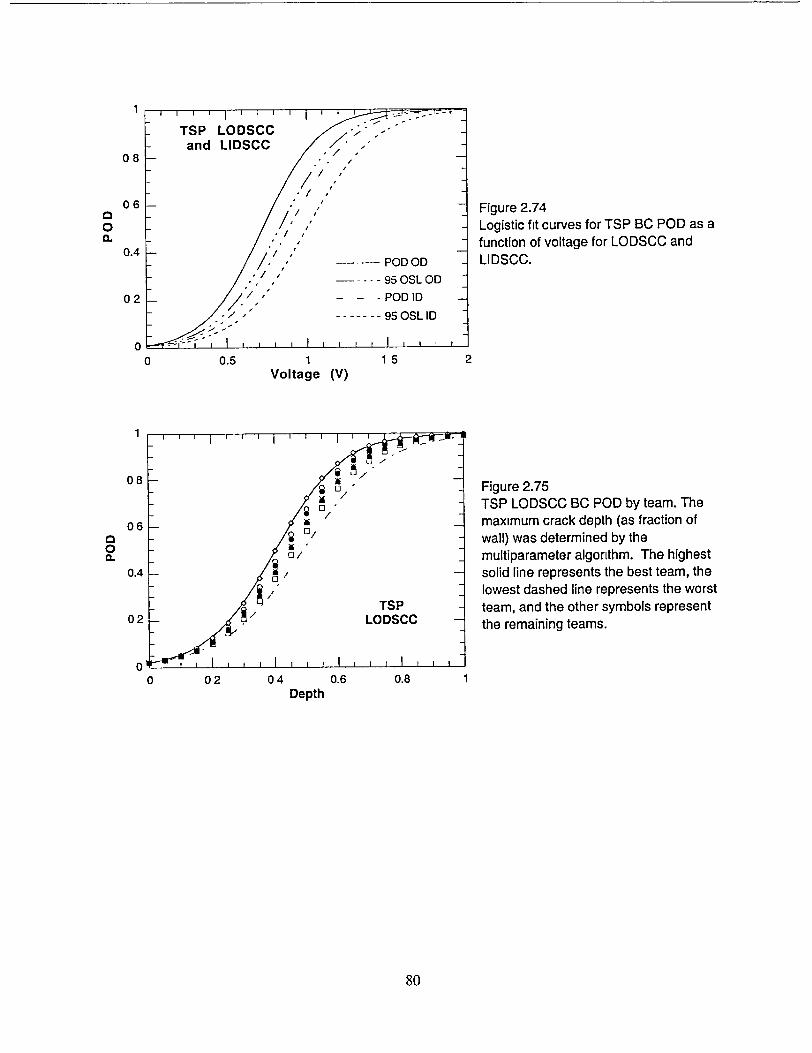
1

08 .''

06 ."/ Figure 2.74

0 •," Logistic fit curves for TSP BC POD as a a. ,function of voltage for LODSCC and

0.4 PODOD LIDSCC.

/ ---- 95OSLOD

02 .. POD ID

----- 95 OSL ID

0 0 0.5 1 15 2

Voltage (V)

08 t / 08 Figure 2.75

TSP LODSCC BC POD by team. The

06 - maximum crack depth (as fraction of O wall) was determined by the 0~ IL •o/ multiparameter algorithm. The highest

0.4 - solid line represents the best team, the

/ Tlowest dashed line represents the worst TSP team, and the other symbols represent

02 20DSCC the remaining teams.

0 I 0 I 0 1 n o 2 0 4 0.6 0.81

Depth

80

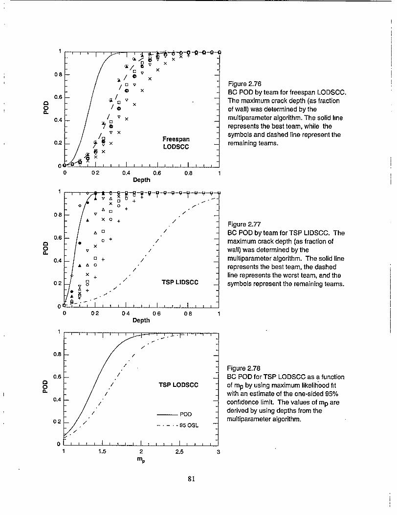
1

08 / 0 v - Figure 2.76

o. X BC POD by team for freespan LODSCC. 0.6 - / V - The maximum crack depth (as fraction

X0of wall) was determined by the

0.4 / v x multiparameter algorithm. The solid line a -represents the best team, while the

/ Vx symbols and dashed line represent the 0.2 -. /9Freespan

02/vxLODSCC remaining teams.

A1,x o I I

0 02 0.4 0.6 0.8 1 Depth

08 o + " 0 A X 0 + / Figure 2.77

- 0 / BC POD by team for TSP LIDSCC. The 0.6 o 0+ maximum crack depth (as fraction of o X

0 v X-wall) was determined by the 0.4 + /- multiparameter algorithm. The solid line

X/ represents the best team, the dashed X+- line represents the worst team, and the

- 0 t TSP LIDSCC symbols represent the remaining teams.

0o I II 0 02 04 06 08

Depth

0.8

Figure 2.78 0.6 - BC POD for TSP LODSCC as a function

0 / TSP LODSCC of mp by using maximum likelihood fit "" with an estimate of the one-sided 95%

0.4 - confidence limit. The values of mp are

/ / ..... POD derived by using depths from the 02 / multiparameter algorithm. 0 2 -./. . .950OSL

1 I I , I I i I i , , i 11.5 2 2.5 3

81

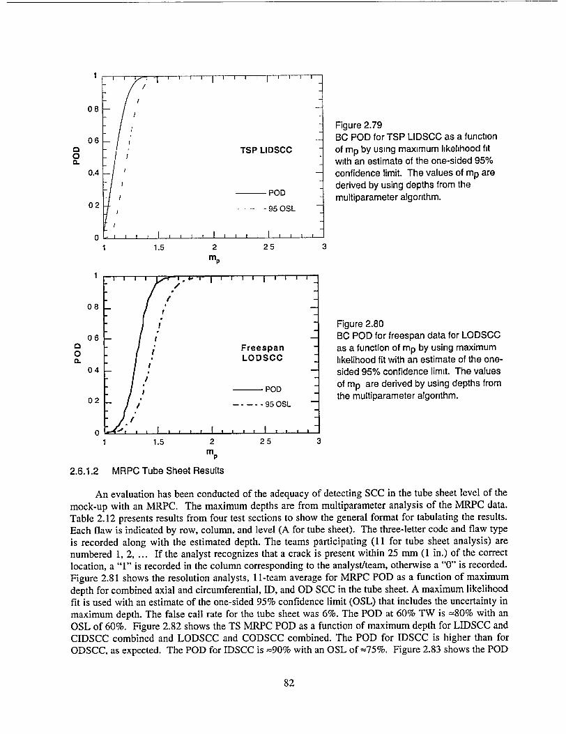
1

08

Figure 2.79

06 BC POD for TSP LIDSCC as a function TSP LIDSCC of mp by using maximum likelihood fit

C.. with an estimate of the one-sided 95% 0.4 confidence limit. The values of mp are

derived by using depths from the -POD multiparameter algorithm.

02 -- -- 95 OSL

0

1 1.5 2 25 3

"M,

08

Figure 2.80 06 " BC POD for freespan data for LODSCC

0 o Freespan - as a function of mp by using maximum

C. LODSCC likelihood fit with an estimate of the one04t

04 sided 95% confidence limit. The values

POD of mp are derived by using depths from

02 the multiparameter algorithm. / ---. 9505SL

0 1 1.5 2 25 3

m P

2.6.1.2 MRPC Tube Sheet Results

An evaluation has been conducted of the adequacy of detecting SCC in the tube sheet level of the mock-up with an MRPC. The maximum depths are from multiparameter analysis of the MRPC data. Table 2.12 presents results from four test sections to show the general format for tabulating the results. Each flaw is indicated by row, column, and level (A for tube sheet). The three-letter code and flaw type is recorded along with the estimated depth. The teams participating (11 for tube sheet analysis) are numbered 1, 2, ... If the analyst recognizes that a crack is present within 25 mm (1 in.) of the correct location, a "1" is recorded in the column corresponding to the analyst/team, otherwise a "0" is recorded. Figure 2.81 shows the resolution analysts, 11-team average for MRPC POD as a function of maximum depth for combined axial and circumferential, ID, and OD SCC in the tube sheet. A maximum likelihood fit is used with an estimate of the one-sided 95% confidence limit (OSL) that includes the uncertainty in maximum depth. The false call rate for the tube sheet was 6%. The POD at 60% TW is =80% with an

OSL of 60%. Figure 2.82 shows the TS MRPC POD as a function of maximum depth for LIDSCC and CIDSCC combined and LODSCC and CODSCC combined. The POD for IDSCC is higher than for ODSCC, as expected. The POD for IDSCC is =90% with an OSL of =75%. Figure 2.83 shows the POD

82

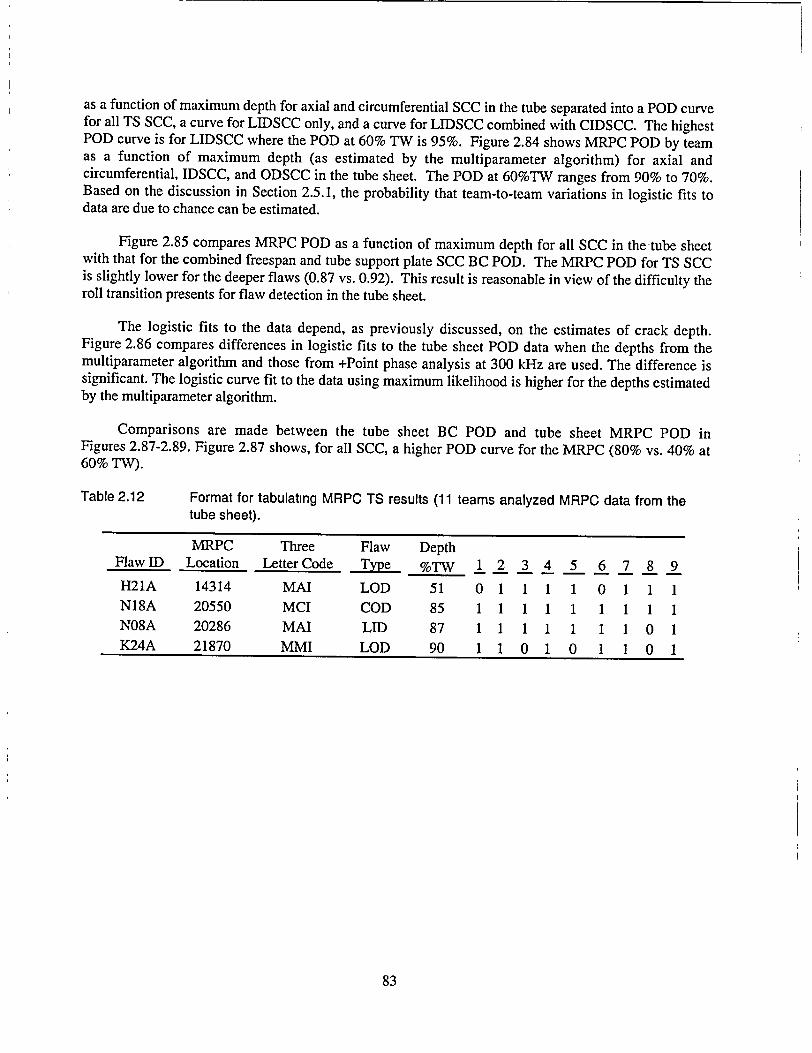
as a function of maximum depth for axial and circumferential SCC in the tube separated into a POD curve for all TS SCC, a curve for LIDSCC only, and a curve for LIDSCC combined with CIDSCC. The highest POD curve is for LIDSCC where the POD at 60% TW is 95%. Figure 2.84 shows MRPC POD by team as a function of maximum depth (as estimated by the multiparameter algorithm) for axial and circumferential, IDSCC, and ODSCC in the tube sheet. The POD at 60%TW ranges from 90% to 70%. Based on the discussion in Section 2.5.1, the probability that team-to-team variations in logistic fits to data are due to chance can be estimated.

Figure 2.85 compares MRPC POD as a function of maximum depth for all SCC in the-tube sheet with that for the combined freespan and tube support plate SCC BC POD. The MRPC POD for TS SCC is slightly lower for the deeper flaws (0.87 vs. 0.92). This result is reasonable in view of the difficulty the roll transition presents for flaw detection in the tube sheet.

The logistic fits to the data depend, as previously discussed, on the estimates of crack depth. Figure 2.86 compares differences in logistic fits to the tube sheet POD data when the depths from the multiparameter algorithm and those from +Point phase analysis at 300 kHz are used. The difference is significant. The logistic curve fit to the data using maximum likelihood is higher for the depths estimated by the multiparameter algorithm.

Comparisons are made between the tube sheet BC POD and tube sheet MRPC POD in Figures 2.87-2.89. Figure 2.87 shows, for all SCC, a higher POD curve for the MRPC (80% vs. 40% at 60% TW).

Table 2.12 Format for tabulating MRPC TS results (11 teams analyzed MRPC data from the tube sheet).

MRPC Three Flaw Depth FlawID Location Letter Code Type %TW 1 2 3 4 5 6 7 8 9 H21A 14314 MAI LOD 51 0 1 1 1 1 0 1 1 1 N18A 20550 MCI COD 85 1 1 1 1 1 1 1 1 1 NOSA 20286 MAI LID 87 1 1 1 1 1 1 1 0 1 K24A 21870 MMI LOD 90 1 1 0 1 0 1 1 0 1

83

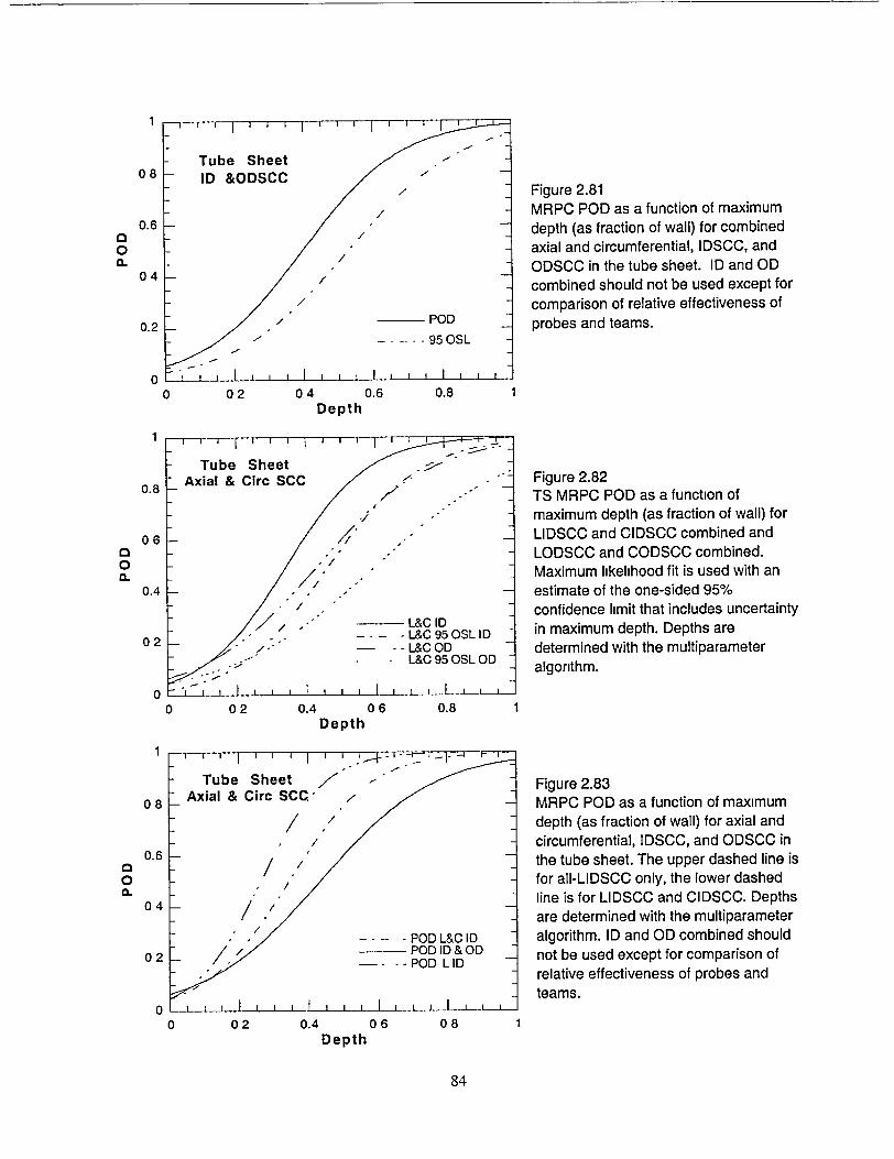
1

08 ID &OD/ / Figure 2.81

MRPC POD as a function of maximum 0.6 - depth (as fraction of wall) for combined

0 axial and circumferential, IDSCC, and .4 ODSCC in the tube sheet. ID and OD

o 4 combined should not be used except for

comparison of relative effectiveness of

0.2 - POD probes and teams. - -_- - -95 OSL

0 1 I I I I I i j

0 02 04 0.6 0.8 1 Depth

Tube Sheet 08 Axial & Circ CC Figure 2.82

0.8 ATS MRPC POD as a function of maximum depth (as fraction of wall) for

06 LIDSCC and CIDSCC combined and , .LODSCC and CODSCC combined.

o Maximum likelihood fit is used with an

0.4 estimate of the one-sided 95%

confidence limit that includes uncertainty - --" - L&C ID in maximum depth. Depths are 0 2~ . . . L&C 95 OSL ID in m x

-. -L&C OD determined with the multiparameter L&C 95 OSL OD algorithm.

0 02 0.4 06 0.8 1

Depth

Tube Sheet Figure 2.83

0 8 Axial & Circ SCC" MRPC POD as a function of maximum depth (as fraction of wall) for axial and

/ circumferential, IDSCC, and ODSCC in 0.6 the tube sheet. The upper dashed line is

0 " for all-LIDSCC only, the lower dashed 04 'line is for LIDSCC and CIDSCC. Depths

are determined with the multiparameter

S. - -POD L&C ID algorithm. ID and OD combined should 0 -- POD ID & OD not be used except for comparison of

relative effectiveness of probes and teams.

0 02 0.4 06 08 1 Depth

84

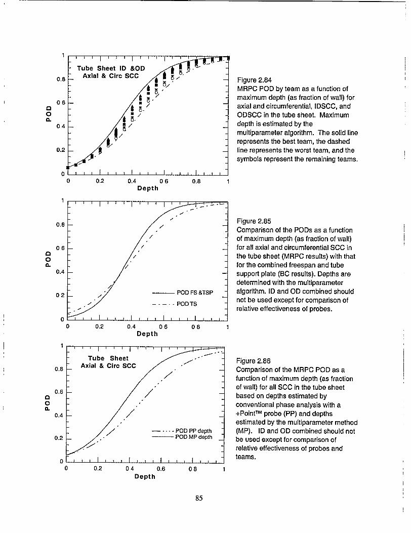
1

0.8 N 0z Figure 2.84 MRPC POD by team as a function of

06 / maximum depth (as fraction of wall) for

o / axial and circumferential, IDSCC, and o ODSCC in the tube sheet. Maximum

04 depth is estimated by the multiparameter algorithm. The solid line represents the best team, the dashed

0.2 line represents the worst team, and the symbols represent the remaining teams.

0 0 0.2 0.4 06 0.8 1

Depth

Figure 2.85 Comparison of the PODs as a function

of maximum depth (as fraction of wall)

0 6 - for all axial and circumferential SCC in 0 /the tube sheet (MRPC results) with that 0 I. for the combined freespan and tube

0.4 support plate (BC results). Depths are

determined with the multiparameter

02 ... POD FS &TSP algorithm. ID and OD combined should

z.... PODTS not be used except for comparison of ... relative effectiveness of probes.

o 0 I I 0 0.2 0.4 06 08 1

Depth

Tube Sheet - T be hee Figure 2.86

0. Axial & Circ SCC .Fiue28

0.8 AxiComparison of the MRPC POD as a function of maximum depth (as fraction of wall) for all SCC in the tube sheet 0.6

0.6 based on depths estimated by 0 conventional phase analysis with a

0.4 +PointTM probe (PP) and depths estimated by the multiparameter method

7-"- -o POD PP depth (MP). ID and OD combined should not 0.2 POD MP depth be used except for comparison of

relative effectiveness of probes and teams.

0 0.2 04 0.6 08 1 Depth

85

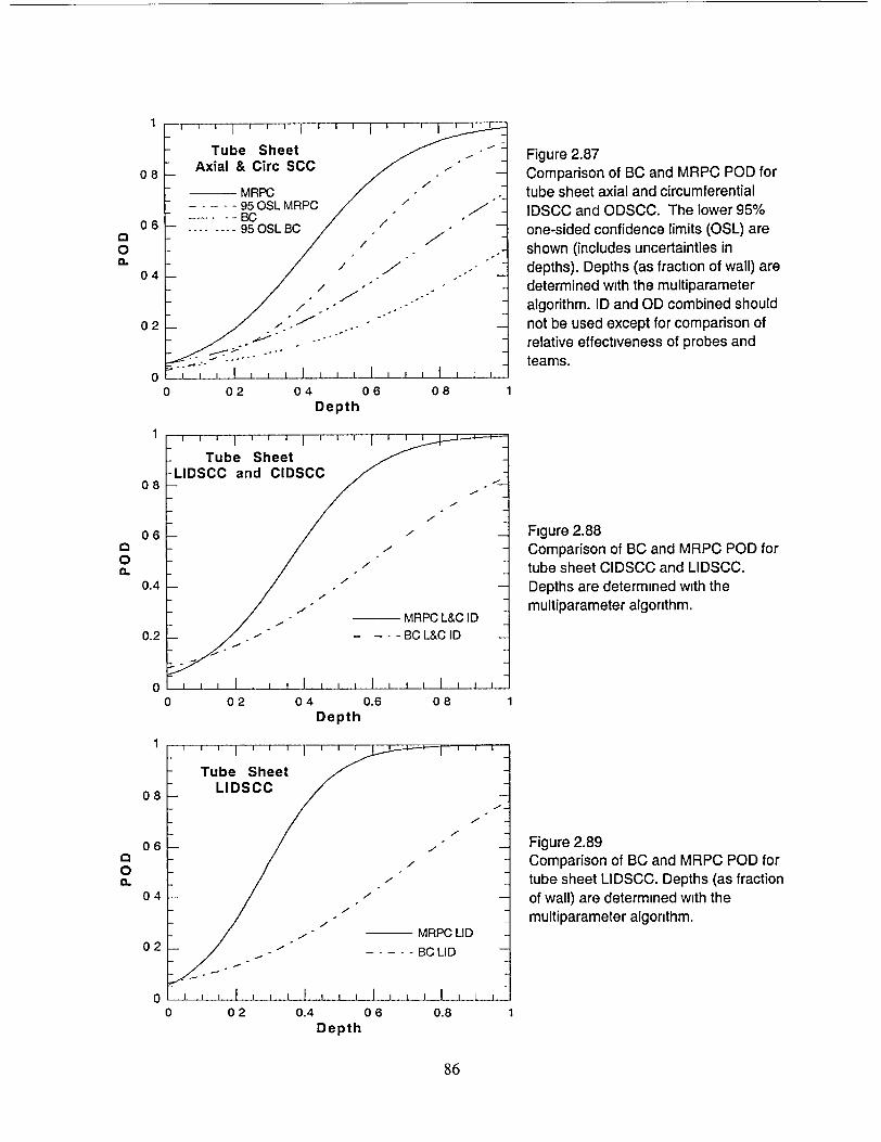
08

06

04

02

0

08

06

0.4

0.2

0

04 06 Depth

08

1

1

Figure 2.88 Comparison of BC and MRPC POD for tube sheet CIDSCC and LIDSCC. Depths are determined with the multiparameter algorithm.

0 02 04 0.6 08 Depth

0 02 0.4 06 0.8 Depth

Figure 2.89 Comparison of BC and MRPC POD for tube sheet LIDSCC. Depths (as fraction of wall) are determined with the multiparameter algorithm.

I

86

Tube Sheet Axial & Circ SCC

- -__ MRPC . 95OSLMRPC

--- BC -9------g95OSLBC

/ / - ° oo °

Figure 2.87 Comparison of BC and MRPC POD for tube sheet axial and circumferential IDSCC and ODSCC. The lower 95% one-sided confidence limits (OSL) are shown (includes uncertainties in depths). Depths (as fraction of wall) are determined with the multiparameter algorithm. ID and OD combined should

not be used except for comparison of relative effectiveness of probes and teams.

0 02

a 0 0.

a 0 CL

0 0 a.

1

08

06

04

02

0

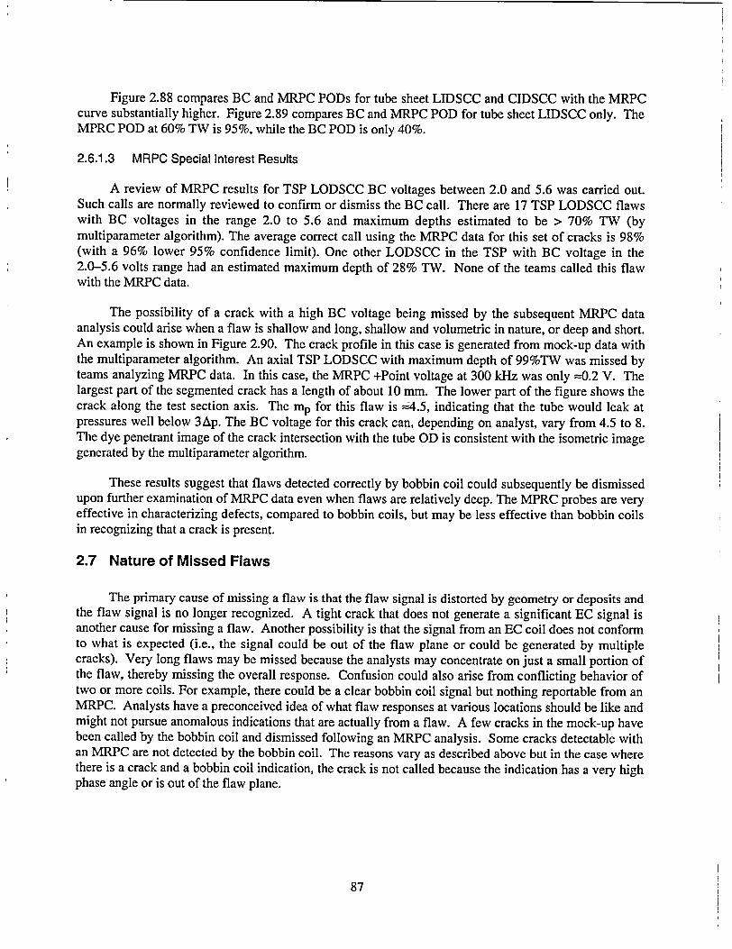
Figure 2.88 compares BC and MRPC PODs for tube sheet LIDSCC and CIDSCC with the MRPC curve substantially higher. Figure 2.89 compares BC and MRPC POD for tube sheet LIDSCC only. The MPRC POD at 60% TW is 95%, while the BC POD is only 40%.

2.6.1.3 MRPC Special Interest Results

A review of MRPC results for TSP LODSCC BC voltages between 2.0 and 5.6 was carried out. Such calls are normally reviewed to confirm or dismiss the BC call. There are 17 TSP LODSCC flaws with BC voltages in the range 2.0 to 5.6 and maximum depths estimated to be > 70% TW (by multiparameter algorithm). The average correct call using the MRPC data for this set of cracks is 98% (with a 96% lower 95% confidence limit). One other LODSCC in the TSP with BC voltage in the 2.0-5.6 volts range had an estimated maximum depth of 28% TW. None of the teams called this flaw with the MIRPC data.

The possibility of a crack with a high BC voltage being missed by the subsequent MRPC data analysis could arise when a flaw is shallow and long, shallow and volumetric in nature, or deep and short. An example is shown in Figure 2.90. The crack profile in this case is generated from mock-up data with the multiparameter algorithm. An axial TSP LODSCC with maximum depth of 99%TW was missed by teams analyzing MRPC data. In this case, the MRPC +Point voltage at 300 kHz was only =0.2 V. The largest part of the segmented crack has a length of about 10 mm. The lower part of the figure shows the crack along the test section axis. The mp for this flaw is =4.5, indicating that the tube would leak at pressures well below 3Ap. The BC voltage for this crack can, depending on analyst, vary from 4.5 to 8. The dye penetrant image of the crack intersection with the tube OD is consistent with the isometric image generated by the multiparameter algorithm.

These results suggest that flaws detected correctly by bobbin coil could subsequently be dismissed upon further examination of MRPC data even when flaws are relatively deep. The MPRC probes are very effective in characterizing defects, compared to bobbin coils, but may be less effective than bobbin coils in recognizing that a crack is present.

2.7 Nature of Missed Flaws

The primary cause of missing a flaw is that the flaw signal is distorted by geometry or deposits and the flaw signal is no longer recognized. A tight crack that does not generate a significant EC signal is another cause for missing a flaw. Another possibility is that the signal from an EC coil does not conform to what is expected (i.e., the signal could be out of the flaw plane or could be generated by multiple cracks). Very long flaws may be missed because the analysts may concentrate on just a small portion of the flaw, thereby missing the overall response. Confusion could also arise from conflicting behavior of two or more coils. For example, there could be a clear bobbin coil signal but nothing reportable from an MRPC. Analysts have a preconceived idea of what flaw responses at various locations should be like and might not pursue anomalous indications that are actually from a flaw. A few cracks in the mock-up have been called by the bobbin coil and dismissed following an MRPC analysis. Some cracks detectable with an MRPC are not detected by the bobbin coil. The reasons vary as described above but in the case where there is a crack and a bobbin coil indication, the crack is not called because the indication has a very high phase angle or is out of the flaw plane.

87

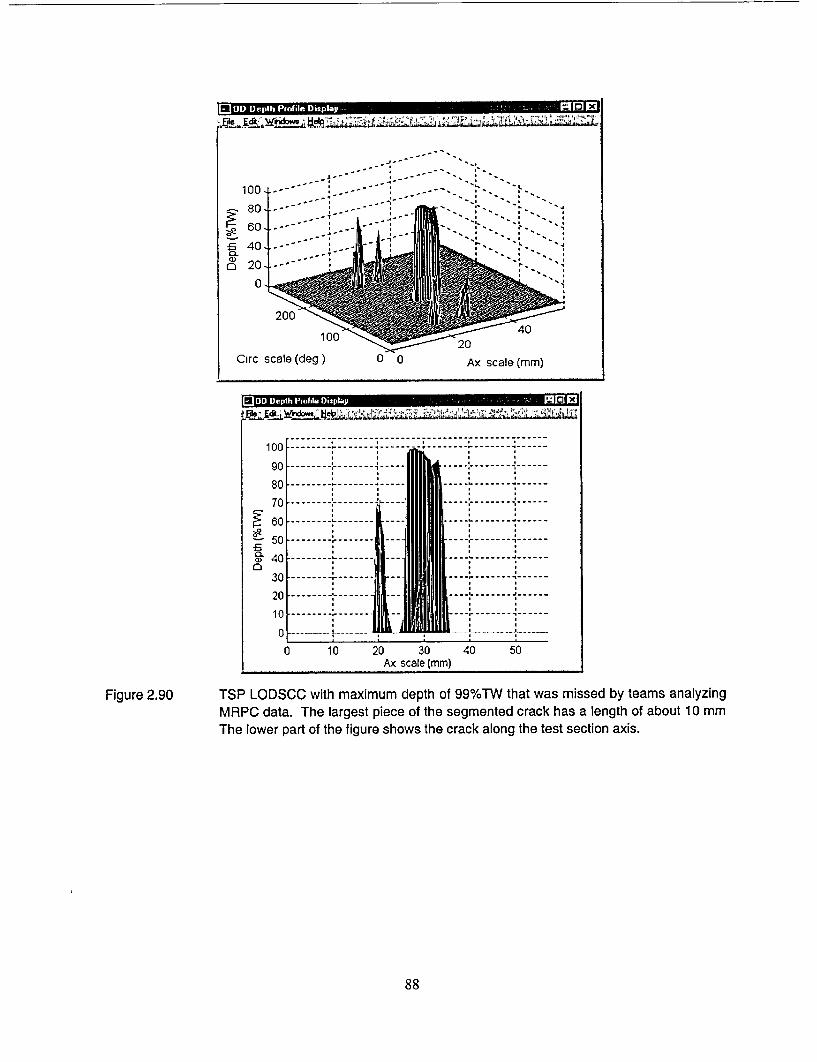
wEml OD Depth I R

IE] .OD Det Flt ipa 1c - j RE

TSP LODSCC with maximum depth of 99%TW that was missed by teams analyzing MRPC data. The largest piece of the segmented crack has a length of about 10 mm The lower part of the figure shows the crack along the test section axis.

88

lie . ---# " 48 I-° d" ' " " ' "

10011----.

20 0

200 100 20 40

Clrc scale (deg) 0 0 Ax scale (ram)

-- - - -.. . .. ... -- .. . . -- - - -.. . . . - -- -- ---. . - ------ - ---- -- - -.

100 -.......................

90 - --- -

0

80 ---- --- -- - --- --- ---- ----.- ----.- --

70 -- - - --- - - - -- - - -- ,--- - -I'- -

0.,

a) 40 -- - - - - - - - - -- - --I-- -

60

30 - - - - - - - - - -- ---- -

20

10 - - - -- . . ----10 . . .... .......... .

0 10 20 30 40 50 Ax scale (mm)

Figure 2.90

2.8 Nature of Overcalls

Overcalls are the result of signals from certain coils that tend to generate flaw-like signals from

geometrical distortions and deposits. Overcalls could also be the result of confusion from conflicting behavior of two or more coils. In a round-robin exercise, there is a tendency to make calls that might not be made under field conditions because there is no penalty for overcalling as long as the overcalling is not

abused. In fact, the reports from resolution analysts show a reasonably low overcalling rate for the freespan (0.1%) and TSP (1.7%). The overcalling in the tube sheet level is significantly higher (6%). The complex nature of the roll transition is probably the root cause of the tube sheet overcalling, although upon further review and destructive analysis, it is possible that unintentional flaws may have been introduced to the tube sheet level during tube expansion, flaw fabrication, and assembly.

89

3 Summary

The mock-up has been shown to have flaws similar to those in operating steam generators, and the round-robin (RR) exercise has successfully mimicked an in-service inspection from preparation of documentation, to collection of bobbin coil and motorized rotating pancake coil (BC and MRPC) data to analysis of the data by qualified teams. Eleven teams have participated in the steam generator RR exercise. The resolution analysts' reports have been used to provide estimates of probability of detection (POD) for some flaw morphologies. The feasibility of determining the reference state, that is, estimating the maximum depth, average depth, area, and mp from the eddy current profile of mock-up flaws has been validated through fractography of laboratory samples containing cracks with various morphologies similar to those in the mock-up. Nevertheless, for the final analysis, the "true" size of some flaws will be determined through destructive examination (NDE). The current NDE study validation effort has led to POD estimates for axial and circumferential inner and outer diameter stress corrosion cracking (ID and OD SCC), shallow to deep. For the flaws analyzed, the mock-up POD is generally high for the deeper freespan and tube support plate (TSP) SCC. However, as noted previously, noise levels in the mock-up are generally less than can be found in field data. Noise as severe as that in the U-bends of plants such as Indian Point 2 was not present in the mock-up freespan and TSP levels.

The possibility of a flaw being detected by BC and dismissed as a flaw by further MPRC evaluations has been demonstrated in this exercise. This situation can occur even when flaws are relatively deep. The MPRC probes are more effective in characterizing defects than are BCs, but the results of the RR exercise do not show any improvement in POD by supplemental rotating probe examinations when following "I" code calls made with the bobbin coil. This is logical because the POD for bobbin calls requiring a supplemental MRPC analysis is simply the probability determined from the two PODs, both of which are less than 1. The combined POD (BC followed by MRPC) = (POD BC) x (POD supplemental MRPC). The flaws missed by the BC examination are not reviewed by an MRPC. Because some of the flaws correctly called by the bobbin coil are now going to be incorrectly dismissed by the MRPC examination, the combined POD is less than the BC POD alone. Note that for the tube sheet where all test sections were examined by MRPC and BC, the MRPC POD is higher than the BC POD (see Figs. 2.87-2.89) Also, signals from geometry in the tube sheet area can lead to significant overcalling although generally the number of overcalls was not particularly high.

Most of the cracks in the mock-up are deep as determined by the application of the multiparameter algorithm. The uncertainty in depth and the skewing toward deeper cracks is accounted for in the confidence limits associated with POD curves.

3.1 Bobbin Coil Results

Estimates of maximum depth from crack profiles and false call rates were used to establish POD as a function of crack depth and mp and to generate logistic curve fits to the data. The NDE uncertainty in depth is included in the one sided 95% lower confidence limit (OSL). In general, the curves have a reasonable shape and thus provide plausible PODs (increasing POD with increasing depth). As expected, the POD for TSP ID cracks is higher than for OD cracks (99% with 98% OSL at 60% TW vs. 75% with 65% OSL at 60% TW). While as expected, the POD for freespan LODSCC (95% at 60% TW) is higher than the POD for TSP LODSCC (75% at 65% TW), it is lower than the POD for TSP LIDSCC (98% at 60% TW). The logistic fit when depths are estimated by ANL's multiparameter algorithm were compared with the fit when the +Point maximum depth estimates are used. Use of the +Point data results in a more conservative POD curve.

90

I

In addition to examination of the RR data as a function of flaw depth, the POD has been evaluated as a function of BC voltage for TSP LODSCC. A pattern similar to that found for POD versus depth is observed for the POD vs. TSP bobbin coil voltage. In this case (POD vs. voltage), the POD curve for LIDSCC at the TSP is lower than that for LODSCC. The lower POD curve for LIDSCC vs. POD for LODSCC, when POD is plotted against voltage, is possibly the result of missing shallow cracks that are in dents with high voltages.

The results were analyzed by team to determine whether there were strong team-to-team variations in the POD. The performances of most of the teams cluster rather tightly, although in some cases there is a significant variation between best and worst. The probability that team-to-team variations in logistic fits to data are due to chance can be estimated. For LIDSCC at the TSP, the variation from best to worst is very significant statistically. There is <0.1% probability that the difference is due to chance (DTC). For FS OD, the variation from best to worst is probably significant (DTC is <20%). For TSP OD, the probability that the variation from best to worst is DTC > 60% and thus the variation is probably not significant.

3.2 Tube Sheet MRPC Results

The POD for SCC in the tube sheet level of the mock-up with an MRPC has been calculated. The maximum-likelihood logistic fit as a function of depth is presented in this report. For all TS POD curves, a false call rate of 6% was used. One-sided 95% OSLs that included uncertainties in maximum depth were also presented.

For MRPC in the tube sheet, the POD for IDSCC is =90%, with an OSL of =75%. The highest POD curve is for LIDSCC where the POD at 60% TW is 95%. MRPC POD by team was presented for axial and circumferential, IDSCC, and ODSCC in the tube sheet. The POD at 60% TW ranges from 90 to 70%.

Comparisons were made between the tube sheet BC POD and tube sheet MRPC POD. For all SCC, there is a higher POD curve for the MRPC (80 vs. 40% at 60% TW). For tube sheet LIDSCC only. the MPRC POD at 60% TW is 95%, while the BC POD is only 40%. For the tube sheet, the MPRC is clearly the probe of choice for detection of SCC. The complication of the roll transition and the presence of circumferential SCC make separating the crack signals from geometry difficult when using a bobbin coil.

3.3 MRPC Analysis of TSP Signals.

A review of MRPC results for BC voltage between 2.0 and 5.6 was carried out. Such calls are normally reviewed to confirm or dismiss the BC flaw call. The result for LODSCC >74% TW is an average correct call of 98%. All teams missed an LODSCC at the TSP with an estimated maximum depth of 28% TW. There is a possibility of having a strong BC signal and a weak MRPC signal that would not be called a crack by analysts. The example presented had an estimated maximum depth of 99% TW with only a few tenths of a volt generated by the +Point coil at 300 kHz. This situation could arise when a flaw is shallow and long or shallow and volumetric in nature or short and tight.

91

3.4 Accuracy of Maximum Depth for Mock-Up Cracks

Accuracy in estimating the maximum depth of cracks in the mock-up was determined from a comparison of crack profiles generated by using ANL's multiparameter algorithm with profiles determined from fractography. The overall RMSE for all cracks of all depths is 15.1%, but there is a significant variation in the RMSE with depth. The RMSE value is significantly better for 80-100% TW cracks than for cracks with other depths.

In Table 2.3, two sets of RMSE values are given. One set is based on the values obtained directly from the multiparameter algorithm and the other on "corrected" values obtained from the regression fit shown in Fig. 2.41. For the shallowest cracks, the "corrected" values give a significantly lower RMSE value, but when all the data are considered the differences in the RMSE for corrected and uncorrected predictions are small. This indicates that there is little systematic bias in the predictions of the multiparameter algorithm, i.e., the errors are random.

These sizing-accuracy results can be used to estimate the uncertainty in POD curves if the multiparameter algorithm is used to determine the "true" state of the mock-up for the NDE round-robin. Instead of characterizing the error in the depths in terms of the overall average for all depths (=15%), the error was taken as a function of depth. Analytically, the values of RMSE given in Table 2.3 are assumed to apply at the midpoint of the depth range for each bin. The error at other depths is then estimated by linear interpolation of these values.

3.5 Overall Capability

The detection capability of current in service inspection (ISI) technology and procedures has been assessed by carrying out an eddy current round-robin (RR) exercise with a steam generator tube bundle mock-up. Inspection of the mock-up and analysis of the data mimicked industry ISI practices conducted on operating steam generators. All documentation for conducting the inspection was prepared with input from an industry-based NDE Task Group, and the realism of the mock-up was established. Data were acquired in June and August 1999 and analysis of the data by 11 commercial teams was completed in December 2000. Each team consisted of five qualified analysts. The exercise took seven to eight working days per team.

The conclusion from the analysis of round-robin results is that good POD can be achieved for deep flaws when commercial techniques are used in a similar manner to that of the RR exercise. The level of success in detection of SCC did vary with flaw location. Estimates of maximum depth from eddy current crack profiles and false call rates were used to establish POD as a function of depth and mp. Logistic fits to the data were generated. The BC POD for TSP ID cracks is higher than for OD cracks (99% with 98% OSL at 60% TW vs. 75% with 65% OSL at 60% TW). The BC POD for freespan LODSCC is =95% at 60% TW. For MRPC in the tube sheet, the POD for IDSCC is =90% with an OSL of =75%. The highest POD curve is for LIDSCC where the POD at 60% TW is 95%. A review of MRPC results for BC voltage between 2.0 and 5.6 was carried out. Such calls are normally reviewed to confirm or dismiss the BC flaw call. The result, for LODSCC > 74% TW is an average correct call of 98%. All teams missed an LODSCC at the TSP with an estimated maximum depth of 28% TW. There is a possibility of having a deep crack with a weak MRPC signal that would not be called a crack by analysts. The example presented had an estimated maximum depth of 99% TW with only a few tenths of a volt generated by the +Point coil at 300 kHz.

92

I

No useful correlation was found between signal amplitude or phase and the maximum depth of the mock-up flaws. When the PODs are considered as a function of mp, it is found that in the TSP and FS regions the POD for cracks that would fail or leak under 3Ap internal pressure (corresponding to mp = 2.3) is >95% even when uncertainties are accounted for.

The adequacy of the multiparameter algorithm for obtaining profiles and maximum depth was established. The results of POD as a function of depth or mp were based on the profiles generated with the multiparameter algorithm.

93

References

1. D. R. Diercks, S. Bakhtiari, K. E. Kasza, D. S. Kupperman, S. Majumdar, J. Y. Park, and W. J. Shack, Steam Generator Tube Integrity Program, Annual Report, October 1999-September 2000, NUREG/CR-651 1, Vol. 8, U.S. Nuclear Regulatory Commission, Washington, DC (2002).

2. S. Bakhtiari, J. Y. Park, D. S. Kupperman, S. Majumdar, and W. J. Shack, Advanced NDE for Steam Generator Tubing, NUREG/CR-6746, U. S Nuclear Regulatory Commission, Washington, DC (2001).

3. S. Majumdar, K. Kasza, and J. Franklin, Pressure and Leak-Rate Tests and Models for Predicting Failure of Flawed Steam Generator Tubes, NUREG/CR-6664 (2000).

4. P. R. Bevington and D. K. Robinson, Data Reduction and Error Analysis for the Physical Sciences, 2nd Ed, McGraw Hill, New York (1992).

5. A. H. Bowker and G. J. Lieberman, Engineering Statistics, Prentice Hall, Englewood Cliffs, NJ (1972).

6. D. A. Powers and Y. Xie, Statistical Methods for Categorical Data Analysis, Academic Press, New York (2000).

94

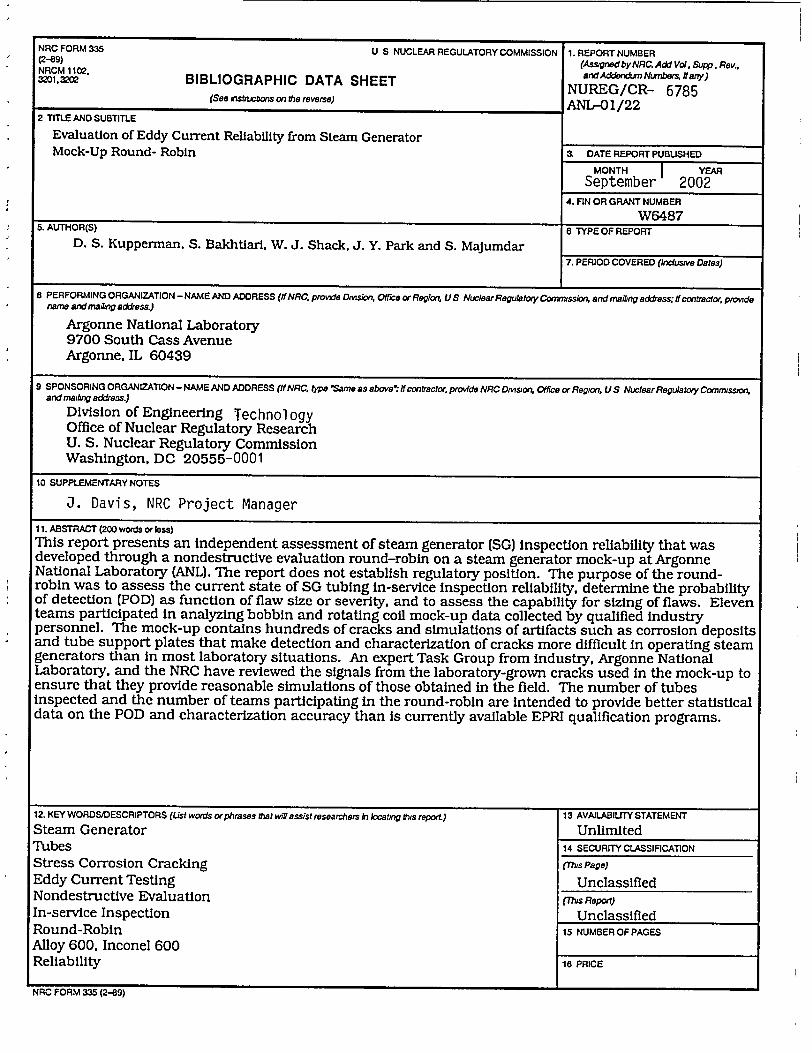
NRC FORM 335 U S NUCLEAR REGULATORY COMMISSION 1. REPORT NUMBER (2-69) (Assigned byNRC. Add Vol, Supp, Rev, NRCM 110•2. and Addendurn Numfbers, #any) NRM1. 2 BIBLIOGRAPHIC DATA SHEET NUREG/CR- 6785

(See mthcons on Me reverse) ANL-01/22 2 TITLE AND SUBTITLE

Evaluation of Eddy Current Reliability from Steam Generator Mock-Up Round- Robin a DATE REPORT PUBUSHED

MONTH I YEAR September 2002

4. FIN OR GRANT NUMBER W6487

5. AUTHOR(S) 6 TYPE OF REPORT

D. S. Kupperman, S. Bakhtiari, W. J. Shack, J. Y. Park and S. Majumdar 7. PERIOD COVERED (Inclusive Dates)

8 PERFORMING ORGANIZATION -NAME AND ADORESS (If NRC, provide Dmsion, Office or Region, US Nuclear Regulatory Conmission, and mailng addess; ff contra.tor provide name and rm ng addies&)

Argonne National Laboratory 9700 South Cass Avenue Argonne. IL 60439

9 SPONSORING ORGANIZATION -NAME AND ADDRESS (If NRC, type 'Same as above', ffcontractor, provide NRC Division. Office orRegion, US Nuclear Regulatory Conrriusslon, and mailung ad&ess.)

Division of Engineering Technol ogy Office of Nuclear Regulatory Research U. S. Nuclear Regulatory Commission Washington, DC 20555-0001

10 SUPPLEMENTARY NOTES

J. Davis, NRC Project Manager

11. ABSTRACT (200 words or less) This report presents an independent assessment of steam generator (SG) inspection reliability that was developed through a nondestructive evaluation round-robin on a steam generator mock-up at Argonne National Laboratory (ANL). The report does not establish regulatory position. The purpose of the roundrobin was to assess the current state of SG tubing In-service inspection reliability, determine the probability of detection (POD) as function of flaw size or severity, and to assess the capability for sizing of flaws. Eleven teams participated in analyzing bobbin and rotating coil mock-up data collected by qualified industry personnel. The mock-up contains hundreds of cracks and simulations of artifacts such as corrosion deposits and tube support plates that make detection and characterization of cracks more difficult in operating steam generators than in most laboratory situations. An expert Task Group from industry, Argonne National Laboratory, and the NRC have reviewed the signals from the laboratory-grown cracks used in the mock-up to ensure that they provide reasonable simulations of those obtained in the field. The number of tubes inspected and the number of teams participating in the round-robin are intended to provide better statistical data on the POD and characterization accuracy than is currently available EPRI qualification programs.

12. KEY WORDS/DESCRIPTORS (Ust words orphrases that MTf7 asist researchers In Iocating ths report) 13 AVAILABILITY STATEMENT

Steam Generator Unlimited Tubes 14 SECURITY CLASSIFICATION Stress Corrosion Cracking (Mrs Page)

Eddy Current Testing Unclassified Nondestructive Evaluation (fMus Repod)

In-service Inspection Unclassified Round-Robin 15 NUMBER OF PAGES Alloy 600, Inconel 600 Reliability 16 PRICE

11m, rwnm 14-cits)

Federal Recycling Program

ISBN 0-16-051217-4

90000

9-780160-512179-

UNITED STATES NUCLEAR REGULATORY COMMISSION

WASHINGTON, DC 20555-0001

OFFICIAL BUSINESS PENALTY FOR PRIVATE USE, $300