Numerical Weather PredictionNumerical Weather Prediction

T-NOTE – Buenos Aires, 5-16 August 2013 –

Juan Ruiz and Celeste Saulo

1

A forecasting system based on numerical weather prediction models

The model:

Numerical core

Parametrizations

Initial

conditions

Lateral boundary

conditions

Post processing

Verification

Parametrizations

Data

assimilation

Observations

-Deterministic run

-Ensemble

Numerical model

Dynamical core:

Equations (including some approximations)

Numerical methods

Physics:

Numerical model components

Physics:

Small scales processes

Typically PBL, convection (sometimes),

microphysics

Uncertainty

Initial conditions:

Imperfect description of the initial state of the system

(atmosphere, land surface, ocean…)

Model error:

Forecast uncertainty

Model error:

Numerics (truncation errors), unresolved scales

(parameterizations), not very well understood processes

Both are important sources of errors in the forecast

Error growth due to the chaotic nature of the atmosphere amplifies

both sources of error.

Which information do numerical models provide about the

occurrence of severe weather events?

NWP can provide information about these events at different spatial

and temporal scales…

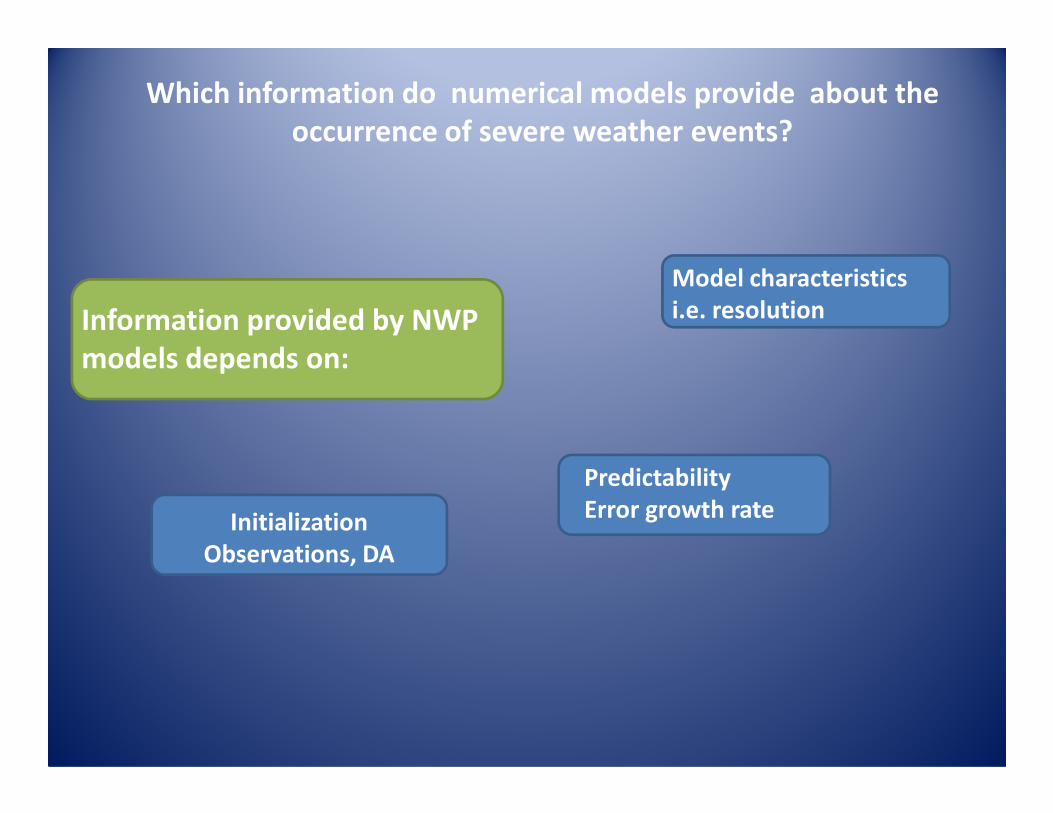
Which information do numerical models provide about the

occurrence of severe weather events?

Information provided by NWP

models depends on:

Model characteristics

i.e. resolution

Initialization

Observations, DA

Predictability

Error growth rate

Model characteristics: resolution

How well do model represent the different phenomena?

Severe weather events are usually associated with meso/micro

scale phenomena:

-Tornadoes-Tornadoes

-Bow-echoes

-Hail

-Persistent heavy rain/ snow fall

-many others …

•Median convective updraft diameters are ~2-4 km

•High resolution models need ~6-8∆∆∆∆ to “resolve” a feature (effective

resolution, model dependent)

Model characteristics: resolutionAre current resolutions enough for the representation of convective

processes?

resolution, model dependent)

Horizontal resolutions between 100-250 m would be needed to

resolve individual convective cells

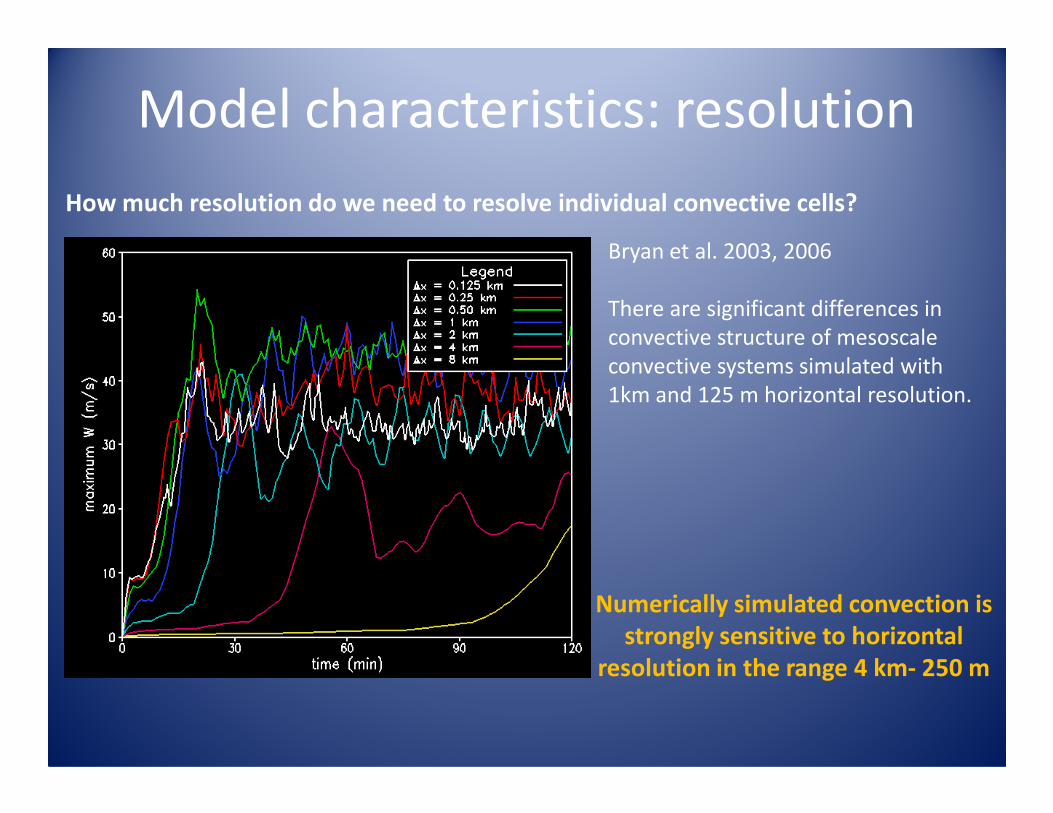
Bryan et al. 2003, 2006

There are significant differences in

convective structure of mesoscale

convective systems simulated with

1km and 125 m horizontal resolution.

Model characteristics: resolution

How much resolution do we need to resolve individual convective cells?

1km and 125 m horizontal resolution.

Numerically simulated convection is

strongly sensitive to horizontal

resolution in the range 4 km- 250 m

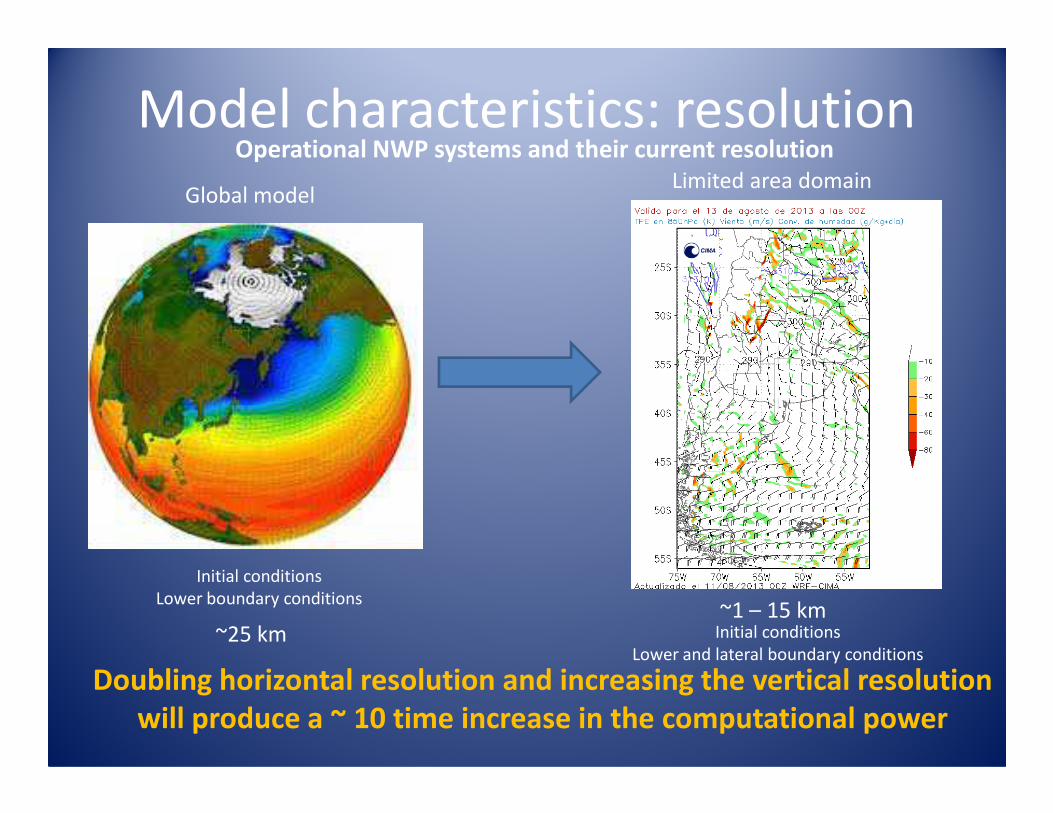
Limited area domainGlobal model

Model characteristics: resolutionOperational NWP systems and their current resolution

Initial conditions

Lower boundary conditions

Initial conditions

Lower and lateral boundary conditions~25 km

~1 – 15 km

Doubling horizontal resolution and increasing the vertical resolution

will produce a ~ 10 time increase in the computational power

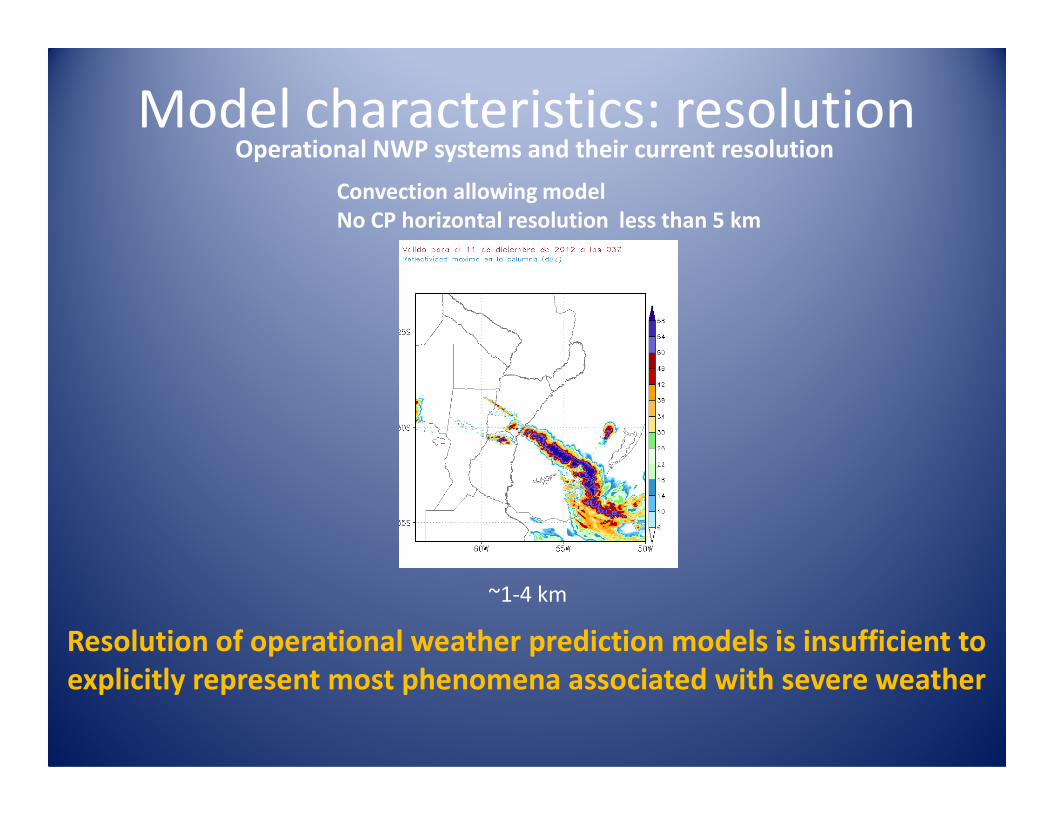
Convection allowing model

No CP horizontal resolution less than 5 km

Model characteristics: resolutionOperational NWP systems and their current resolution

~1-4 km

Resolution of operational weather prediction models is insufficient to

explicitly represent most phenomena associated with severe weather

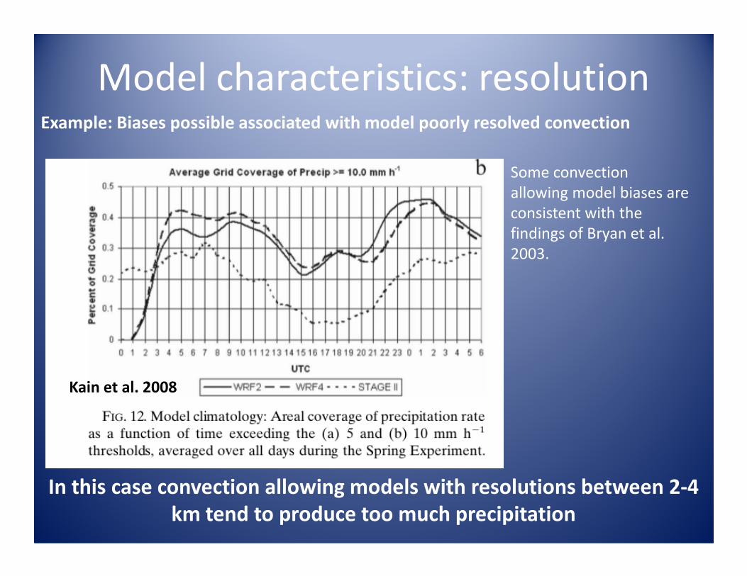
Model characteristics: resolutionExample: Biases possible associated with model poorly resolved convection

Some convection

allowing model biases are

consistent with the

findings of Bryan et al.

2003.

Kain et al. 2008

In this case convection allowing models with resolutions between 2-4

km tend to produce too much precipitation

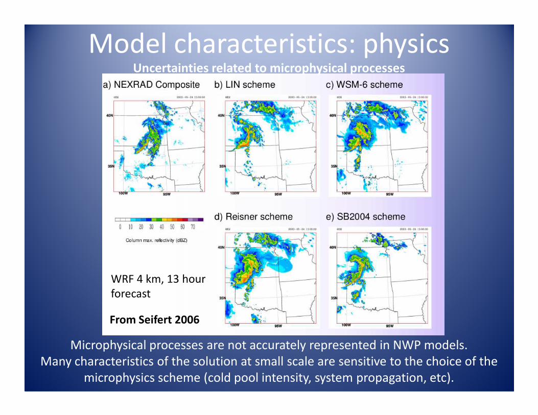
Model characteristics: physicsUncertainties related to microphysical processes

From Seifert 2006

Microphysical processes are not accurately represented in NWP models.

Many characteristics of the solution at small scale are sensitive to the choice of the

microphysics scheme (cold pool intensity, system propagation, etc).

WRF 4 km, 13 hour

forecast

Model characteristics: physicsUncertainties related to boundary layer turbulence

•PBL systematic errors depend on the time of the day and also on the large scale situation.

•These errors will significantly impact convective initiation and evolution as well as its strength.

•Other model errors probably involved (Land surface model biases)

Coniglio et al. 2013 WAF.

Model characteristics: physicsUncertainties related to boundary layer turbulence

Capping inversion under prediction by several PBL schemes in a convection allowing model

Coniglio et al. 2013 WAF.

Predictability

Strongly related to error growth in the forecast

Do all phenomena have the same predictability limit?

Synoptic scale features are usually predictable up to more than 10

days.

Predictability

days.

Error growth is approximately 10 times faster at the mesoscale.

1day lead time roughly equivalent to a 10 day lead time in the synoptic

scale. (Hohenegger and Schar 2007)

At the mesoscale error growth is dependant on its amplitude, the smaller the error

the faster it grows.

Predictability

Zhang et al. 2003

A large improvement of the initial conditions will only produce a short

extension of the predictability limit

Small errors

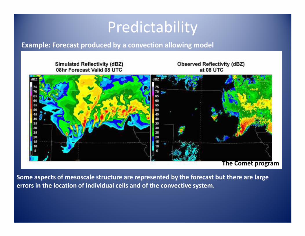
PredictabilityExample: Forecast produced by a convection allowing model

The Comet program

Some aspects of mesoscale structure are represented by the forecast but there are large

errors in the location of individual cells and of the convective system.

FORECAST OBSERVATION

PredictabilityExample: Forecast produced by a convection allowing model

18 hr forecast with 4 km (WRF-Chuva).

Position and / or timing errors can be large, O (100 km) and O ( 1-3 hr )

respectively (in the first 24 hours) and will continue growing with time

Predictability is longer for small scale phenomena associated with land surface forcings or

topography

Predictability

Sea breeze front well represented in the model forecast.

Land sea breezes may be forecasted even without a proper

initialization of the mesoscale in the numerical model, given that the

mesoscale forcing is well represented

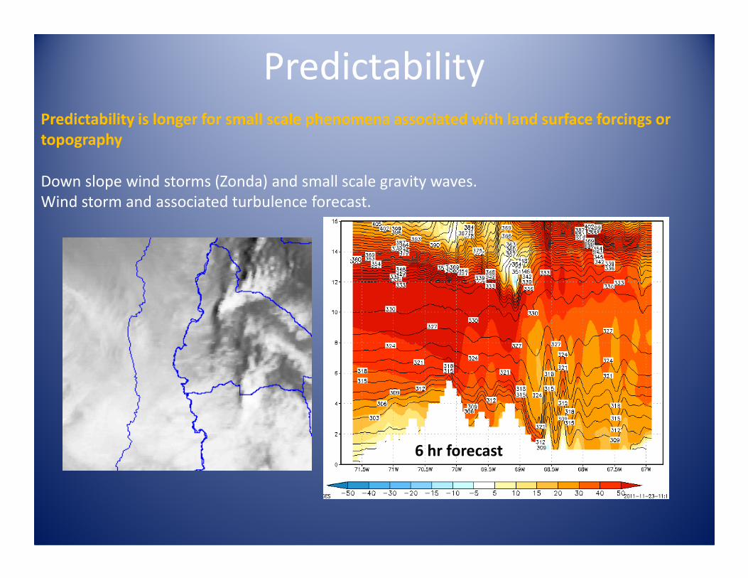
Down slope wind storms (Zonda) and small scale gravity waves.

Wind storm and associated turbulence forecast.

Predictability is longer for small scale phenomena associated with land surface forcings or

topography

Predictability

6 hr forecast

InitializationInitialization deals with the generation of the initial conditions for the forecast

Several data assimilation techniques provide ways to combine observations and

short range forecasts to obtain initial conditions approximately consistent with

model dynamics.

InitializationInitialization strategy depends on the scale of the phenomena that we want to

forecast

Models for synoptic scale prediction are usually initialized every 6

hours using different types of observations (soundings, satellite,

surface, etc)

Models for mesoscale forecasts have to be initialized more frequently

(1 hour to 15 minutes) using dense observational networks , radars

and other observations when they are available.

The smaller the scale the larger the number of observations that we

need and the higher the assimilation frequency.

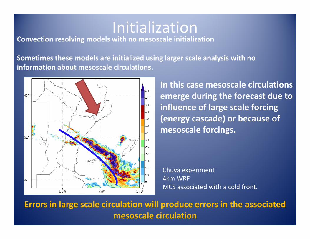
InitializationConvection resolving models with no mesoscale initialization

Sometimes these models are initialized using larger scale analysis with no

information about mesoscale circulations.

In this case mesoscale circulations

emerge during the forecast due to

influence of large scale forcing

(energy cascade) or because of

Chuva experiment

4km WRF

MCS associated with a cold front.

Errors in large scale circulation will produce errors in the associated

mesoscale circulation

(energy cascade) or because of

mesoscale forcings.

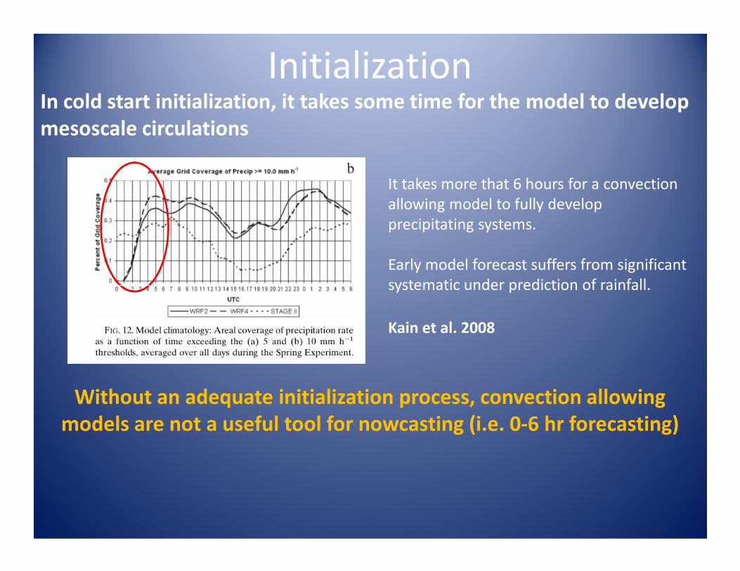
InitializationIn cold start initialization, it takes some time for the model to develop

mesoscale circulations

It takes more that 6 hours for a convection

allowing model to fully develop

precipitating systems.

Early model forecast suffers from significant

systematic under prediction of rainfall.

Kain et al. 2008

systematic under prediction of rainfall.

Without an adequate initialization process, convection allowing

models are not a useful tool for nowcasting (i.e. 0-6 hr forecasting)

Example of convective mode forecast using a

convective allowing model.

(22 hours forecast, 2 km resolution WRF, cold

start).

Kain et al. 2008 WAF.

InitializationCold start initialization:

Kain et al. 2008 WAF.

Mesoscale organization of

convection can be captured even if

the exact position and timing can

not be predicted

Initialization

Mesoscale initialization (Jenny Sun will talk about high resolution data assimilation

on Wednesday)

Radar data assimilation can reduce spin-

up and improve forecast skill for the first

12 hours.

Lightning observations can also provide information to

constrain the small scales.

NWP TOOL FOR NOWCASTING

Low resolution soil moisture High resolution soil moisture

InitializationLand surface initialization also important for convective scale forecasting

Better representation of

precipitation along a dry line.

Probably due to stronger heat

fluxes and stronger convective

rolls in the PBL that help to

trigger convection along the dry

line.

Trier, Chen, and Manning, Mon. Wea. Rev., 2004

Summary

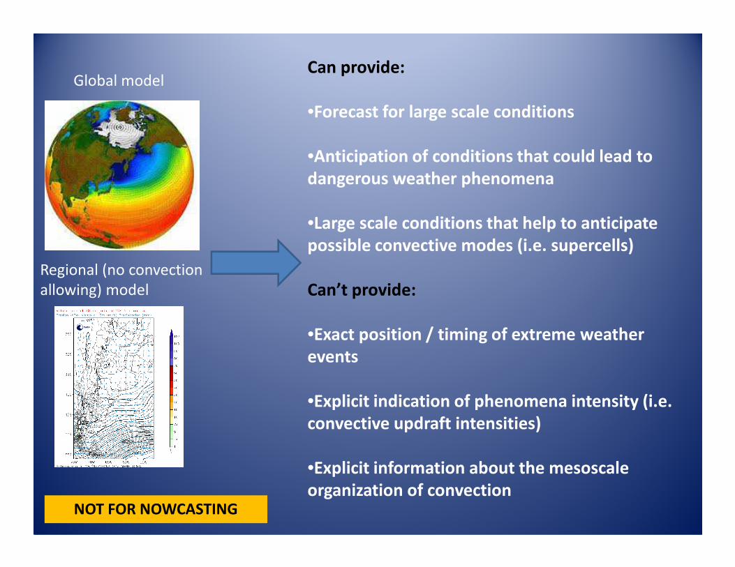
Global model

Regional (no convection

allowing) model

Can provide:

•Forecast for large scale conditions

•Anticipation of conditions that could lead to

dangerous weather phenomena

•Large scale conditions that help to anticipate

possible convective modes (i.e. supercells)

Can’t provide:allowing) model Can’t provide:

•Exact position / timing of extreme weather

events

•Explicit indication of phenomena intensity (i.e.

convective updraft intensities)

•Explicit information about the mesoscale

organization of convectionNOT FOR NOWCASTING

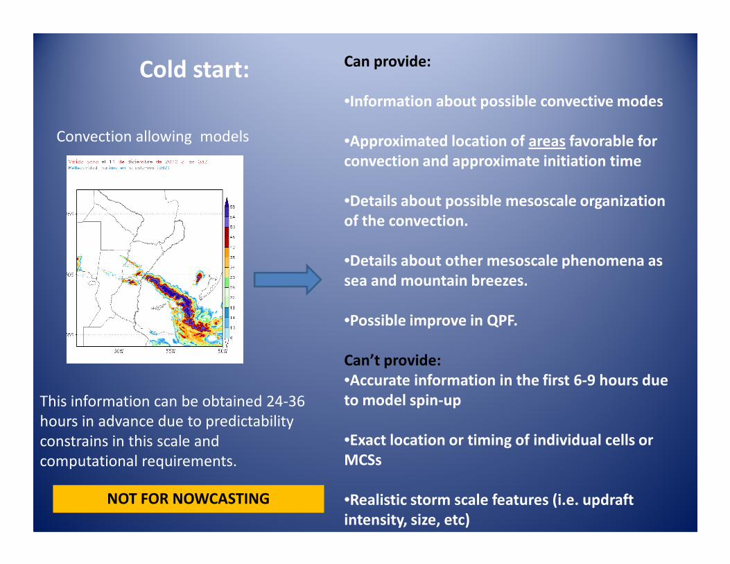
Convection allowing models

Can provide:

•Information about possible convective modes

•Approximated location of areas favorable for

convection and approximate initiation time

•Details about possible mesoscale organization

of the convection.

•Details about other mesoscale phenomena as

sea and mountain breezes.

Cold start:

sea and mountain breezes.

•Possible improve in QPF.

Can’t provide:

•Accurate information in the first 6-9 hours due

to model spin-up

•Exact location or timing of individual cells or

MCSs

•Realistic storm scale features (i.e. updraft

intensity, size, etc)

This information can be obtained 24-36

hours in advance due to predictability

constrains in this scale and

computational requirements.

NOT FOR NOWCASTING

Convection allowing models

Can provide:

•Less spin up issues

•Information about the convective modes

•Approximated location of convection (limited

by predictability issues)

•Details about mesoscale organization of the

convection

Mesoscale initialization:

convection

Can’t provide:

•Realistic storm scale features (i.e. updraft

intensity, size, etc)

Location and timing can be obtained with 1-3 hours in advance due to predictability

constrains at this scale. Skill even more limited by model errors.

NWP BASED NOWCASTING TOOL

Post proccessing

Some high resolution diagnostics for severe weather applications

Convection allowing models are able to generate some features that resemble circulations

associated with observed convective storms as for example mesocyclones that characterize

supercells.

Although cold start convective allowing models won’t provide a detailed location, timing and

strength of these features model outputs can be used as a guidance for evaluation of possible

occurrence.

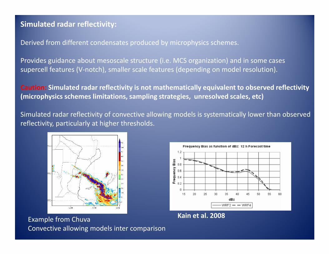
Simulated radar reflectivity:

Derived from different condensates produced by microphysics schemes.

Provides guidance about mesoscale structure (i.e. MCS organization) and in some cases

supercell features (V-notch), smaller scale features (depending on model resolution).

Caution: Simulated radar reflectivity is not mathematically equivalent to observed reflectivity

(microphysics schemes limitations, sampling strategies, unresolved scales, etc)

Simulated radar reflectivity of convective allowing models is systematically lower than observed

reflectivity, particularly at higher thresholds.reflectivity, particularly at higher thresholds.

Kain et al. 2008Example from Chuva

Convective allowing models inter comparison

Updraft helicity:

Vertically integrates the product of updraft intensity and vorticity.

Provides guidance about simulated rotating updrafts.

Caution:

Thresholds are determined empirically to match the simulated frequency of mesocyclones

with the observed frequency. The threshold is resolution dependent!

Different sign combinations might lead to similar results (i.e. rotating downdrafts) or opposite

results (anticiclonically rotating updrafts).

The Comet program Kain et al. 2008

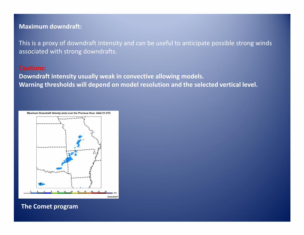
Maximum downdraft:

This is a proxy of downdraft intensity and can be useful to anticipate possible strong winds

associated with strong downdrafts.

Cautions:

Downdraft intensity usually weak in convective allowing models.

Warning thresholds will depend on model resolution and the selected vertical level.

The Comet program

Maximum vertically integrated graupel:

This quantity may be useful for anticipating hail hazard and updraft strength.

Cautions:

Thresholds will depend upon model resolution and microphysics scheme.

The Comet program.

Conclusions:

High resolution (convection allowing models) are useful tools for forecasting areas likely to be

affected by extreme weather events.

They provide information about the mesoscale structure of convection.

They may improve QPF due to a better representation of mesoscale processes.

They can be used as part of a nowcasting system if they are initialized with high resolution

data.

They suffer from very limited predictability, even when initialized with high resolution data.

They suffer from model errors associated with unresolved (or poorly understood) smaller scale

processes.

We suffer as well…