317

International Journal of Mechanical and Materials Engineering (IJMME), Vol.6 (2011), No.3, 317-325

NUMERICAL STUDY ON EFFECT OF REDUCED FREQUENCY ON A VORTEX INDUCED

BY AN OSCILLATING SUB BOUNDARY LAYER VORTEX GENERATOR

K. A. Ahmad School of Aerospace Engineering, Universiti Sains Malaysia, Nibong Tebal 14300 Penang, Malaysia

E-mail: aekamarul@eng.usm.my

Received 1 December 2010, Accepted 25 November 2011

ABSTRACT

This paper presents a numerical study of the effects of

reduced frequency on the performance of an oscillating sub-

boundary layer vortex generator. The numerical simulations

were done using Fluent 6.3 and RANS equations were used

to model the flow field induced by the vortex generator on a

flat plate. A hybrid mesh with SST k-ω turbulence model

was used during the computations. The undisturbed

boundary layer thickness at the location of vortex generator

was 80 mm and a vane-type VG with height of 40 mm was

used. The flow Reynolds number based on the streamwise

distance is 106. The VG was oscillated in a simple harmonic

motion between 0o to 15

o over a range of reduced frequency,

F+. The increase in the spanwise averaged skin friction with

the increase in reduced frequency is clearly observed.

Furthermore, the time averaged skin friction distribution for

oscillating SBVG is less spread compared to the static

SBVG. The results also show that an increase in the reduced

frequency induces secondary vortex to appear. The

simulations result obtained are also found in satisfactory

agreement with the experimental results.

Keywords: Numerical modeling, active flow control,

vortex generator

NOMENCLATURE

c Vortex generator length

fc Skin friction

k Turbulence kinetic energy

Angle of vibration

max Maximum angle of pitch

min Minimum angle of pitch

F+

Reduced frequency

y+ Local Reynolds number

ω Specific turbulent dissipation rate

h Vortex generator’s height

P Period

t time

τ The ratio of time over VG oscillation period

δ Boundary layer thickness

SST Shear Stress Transport

U∞ freestream velocity

ω Specific turbulent dissipation rate

1. INTRODUCTION

Active flow control (AFC) is one of the areas in fluid

mechanics that is hotly being pursued by scientists and

researchers in the current century. The latest comprehensive

review and analysis on the subject was done by Gad El Hak

(2001) and Collis et al (2004). Traditionally, flow control is

confined within passive mode which requires minimal

energy consumption and easy installation. These

conventional devices however are limited to one operational

condition and cannot adapt with the change of operational

conditions (Lin 2002). Active flow control emerged in

response to overcome this barrier.

Generally, AFC involves two types of devices namely air

jets (Kupper and Henry 2003, Ekaterinaris 2004, Shojaefard

et al 2005, Coiro et al 2008) and vibrated flow control

devices (Guo 2008, Kauertz and Neuwerth 2006, Jolibois

and Moreau 2008, Lebeau et al 2007, Benard et al 2009).

The air-jet vortex generator (AJVG) has been proposed

(Kupper and Henry 2003)

as a credible alternative to

conventional vane vortex generator. They presented

streamwise and cross stream velocity profiles to describe the

vortex strength and position. The results indicated that the

downstream behavior of the predicted vortex was largely

unaffected by the shape of the velocity profile of the

incoming jet.

Ekaterinaris (2004) had used pulsating air jet on airfoils and

wings at low speed configurations. Pulsating jet active flow

control was applied as a surface boundary condition and the

flow was time-dependent. The effects of pulsation frequency

and jet exit velocity on flow control gave beneficial impacts

on the oscillation amplitude and three-dimensional profile.

Shojaefard et al (2005) also conducted research on the airjet

device. His mechanism consisted of four suction and

injection slots on the suction side of the airfoil. The results

showed that the surface suction could increase the lift

coefficient; the injection decreased the skin friction.

318

Some investigators used different techniques of blowing.

(Coiro et al 2008) investigated both the steady and

unsteady-blowing techniques as tools for turbulent

separation control. Pulsed blowing depends on two

parameters: reduced frequency and momentum coefficient.

The numerical simulation of a pulsed-blowing system was

conducted to highlight how aerodynamic performance

depended on geometrical parameters to drive the design of

the experimental test. The results showed that this technique

was very effective to delay or suppress separation on a

single component airfoil in the pre-stall configuration,

focusing on cruising conditions. One of researchers that

involved in vibrated flow control devices (Kauertz and

Neuwerth 2006). He used a simple wing model with

winglets which were able to produce a vortex system of up

to six distinct vortices. By means of active oscillation of

rudders integrated into the winglets, these vortex systems

were to be excited to initiate an accelerated decay of the

vortices. Another study about vibrated flow control device

was performed (Jolibois and Moreau 2008)

who used

dielectric barrier discharge plasma tangentially to the wall,

in order to modify velocity in the boundary layer.

Plasma actuators have been studied numerically by IeBaeau

et al (2007) as a potential effective method for boundary

layer control. This boundary layer control device was driven

by a body force vector tangent to the surface where the

actuator was integrated. The result showed that this type of

action was able to fully reattach an airflow naturally

separated, for angles of incidence up to 170. Meanwhile

Mamun et al (2010) investigated the performance of a

moving lid within the trapezoidal cavity on the heat transfer

rate via numerical approach. He found that the aspect ratio

and the direction of the moving lid have significant effects

on the heat transfer rate.

In the current paper, the author studied the effect of reduced

frequency on the vortex induced by an oscillating sub-

boundary layer vortex generator (SBVG). The author has

studied the interaction between a nominally two-

dimensional, turbulent boundary layer, and the embedded

longitudinal vortices generated by a SBVG oscillating about

an axis through its trailing edge. The reduced frequency was

varied in order to monitor its effect on the SBGV, through

the distribution of the skin friction.

2. NUMERICAL METHODS

This study employed the commercial CFD code Fluent

6.3TM

. The incompressible Reynolds-averaged Navier-

Stokes equations were modelled. There are several options

for turbulence models that are available in Fluent but this

investigation focuses on the two-equation model, SST k-.

The software was run in its implicit segrageted mode; the

SIMPLE algorithm was used for pressure-velocity coupling

and second order spatial discretisation was used for all the

equations. A range of time step of 1×10−3

to 2.5×10−4

sec

was used and 60 sub-iterations per time step was performed.

Calculations were run for several cycles, until periodicity

was observed in the solution. The simulations were

performed using the parallel version of Fluent code and this

code uses the Load Sharing Facility (LSF) on 4 parallel

processors. Time taken for most cases took approximately

24 hours.

2.1 Governing equations

The integral form of the transport equation for a general

scalar, F, on an arbitary control volume, V, which

implemented in Fluent 6.3, is as shown below:-

V V Vg

VdVSAdAduudV

dt

d ..

(1)

The first and second terms on the left are the time derivative

term and the convective terms. The time derivative term

indicates that the solution is changing with time. Meanwhile

the first and the second terms on the right of equation 1 are

the diffusive terms and the source terms. The term ∂V is

used to represent the boundary of the control volume V. The

SIMPLE algorithm is available in FluentTM

and was used for

pressure-velocity coupling and second order spatial

discretisation was used for all the equations. The time

derivative in equation 1 can be discretised using equation 2.

t

VVdV

dt

dnn

V

1

(2)

The indices n and n+1 denote, respectively, the quantity at

the current and next time level. Meanwhile the (n+1)th time

level volume Vn+1is computed from equation 3.

tdt

dVVV nn 1

(3)

The term dt

dV denotes the volume time derivative of the

control volume. In order to satisfy the grid conservation law,

the volume time derivative of the control volume is

computed from equation 4.

V

n

j

jgjg

f

AuAdudt

dV .. (4)

The term nf is the number of faces on the control volume and

jA

is the face area vector. The dot product jgj Au

on

each control volume face is identical to the volume swept by

the control volume face j over unit time:

t

VAdu

j

g

(5)

A moving mesh technique, spring-based smoothing method

(Fluent Inc) was employed to allow for oscillation of the

vortex generator boundaries; in order to avoid negative cell

volumes, it was found to be necessary to use tetrahedral cells

around the whole of the vortex generator. The value of y+ for

319

the first cell centre off the wall is about 1. The VG is rotated

about its trailing edge in simple harmonic motion and this

motion is governed by the harmonic equation shown below:

))cos(1)((2

1minmaxmin t

(6)

The frequency was chosen to be in the range of 40 Hz to 160

Hz, and this corresponds to a range of reduced frequency F+

of 4 to 10 (see equation 7).

U

cF

2

(7)

A spring based smoothing method was used to govern the

motion of the mesh. The edges between any two mesh nodes

were idealized as a network of interconnected springs. The

initial spacing of the edges before any boundary node

generates a force proportional to the displacement along all

the springs connected to the node. Using Hook’s law, the

force on a mesh node can be written as

in

j

ijiji xxkF

(8)

where jx

and ix

are the displacements of node i and its

neighbor j, ni is the number of neighboring nodes connected

to node i, and kij is the spring constant (or stiffness) between

node i and its neighbor j. The spring constant for the edge

connecting nodes i and j is defined as

||

1

ij

ijxx

k

(9)

This method is appropriate for triangular type of mesh since

they can easily be idealized as springs.

2.2 Geometry, mesh and boundary conditions

The VG has a root chord of 74.3 mm, a trailing edge span (h)

of 35 mm, and a thickness of 1.5 mm. Figure 1 shows a

single VG and the direction of its motion. The domain has

length, breadth, and depth of 1250 mm × 475 mm × 792 mm,

i.e. 34h × 10h × 20h (see Figure 2). The domain size was

chosen as such in order to obtain a domain independent

solution. The VG was placed 7h downstream of the inflow

boundary. The freestream velocity was set to 5 m/s; a

velocity profile corresponding to a Reynolds number of 106

is applied at the inflow boundary, so that at the VG location,

the undisturbed boundary layer thickness was 2h. Three

downstream locations were identified to present the cross-

flow contour plots and velocity vector plots. These locations

were X1, X2 and X3 and from VG trailing edges were 4c, 6c

and 8c (see Figure 3). A hybrid mesh approach was

employed in order to capture the main features of the

turbulent boundary layer (see Figure 4). The mesh

generation software used is the ICEMCFDTM

. Mesh

dependency check was performed and it was found that the

number of cells of 3.2 × 105 were sufficient to obtain mesh

independency.

Figure 1 Vortex generator motions

Figure 2 Computational Domain and Boundary

Conditions a) Front view b) Side view

320

Figure 3 Lateral locations for flow properties profiles

analysis

Figure 4 Sample of Mesh

2.3 Testing parameters

The simulations involved two types of flow control device

namely static SBVG and oscillated SBVG. The static SBVG

was set to have an angle of attack of 150. The results of the

static SBVG will compared with the experimental results14

.

Meanwhile for the time-dependent case, the SBVG was

oscillated in a range of reduced frequency of 4 to 10, from 00

to +150.

3. RESULTS AND DISSCUSSION

3.1 Embedded steady vortex/boundary layer interaction

A comparison between CFD and experimental results were

made for Reynolds shear stress parameters. Only results

from static SBVG were compared as the experimental

results (Martin 2001) for oscillating SBVG is not available.

Due to the turbulence modelling used in the current study, it

is impossible to obtain exact values of Reynolds shear

stresses. Instead, the Boussinesq eddy-viscosity concept can

be used to provide an estimation of the Reynolds shear

stresses. In an analogous manner to the viscous stresses

caused by mixing of momentum at the molecular level, the

turbulence stresses can be assumed to be proportional to the

mean velocity gradient via an eddy viscosity, . The

Reynolds stresses are estimated through the following

formulae,

y

Ukuu

2

3

2'' (10)

z

Uk

2

3

2'' (11)

x

V

y

Uu '' (12)

x

W

z

Uu '' (13)

y

W

z

V '' (14)

Figure 5 Comparison of Reynolds shear stress 2

/ Uu distribution at X1 (a) CFD (b) Experiment

Figures 5 to 7 show the comparison between the Reynolds

stress predictions and experimental14

results. Figure 5 shows

the primary shear stress, ''u . A distinct feature like an

inverted “mushroom cap” can be observed in Figure 5, both

in CFD and experimental results. The feature is made up of

negative ''u and with a maximum magnitude of -

0.0015. A region of high positive ''u can be observed

in the downwash region of the primary vortex. A maximum

(b)

(a)

321

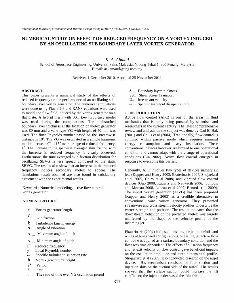
magnitude of 0.0025 is found here and made up from fluid

entrained from the upper region of the boundary layer. In

the experimental results, one can clearly observe the

inverted “mushroom cap”, made up of negative ''u .

One also can observe the region of high positive ''u in

the downwash region. These two similar features suggest

that the predictions of ''u is reasonably correct. Figure

6 shows the secondary shear stress, - ''u . From the CFD

figure, one can see peaks and trough: the trough coincides

with the vortex core and the peaks are disposed the either

sides of it. The peak to the right of the core shows the

largest positive value of ''u . From the Experimental

figure, one can see the similarity of the peaks, and the

trough. The peak to the right of vortex core however, is

likely to be seen as a “tongue”, while this feature is less

obvious in the prediction.

Figure 6 Comparison of Reynolds Shear Stress 2

/ Uwu distribution at X1(a) CFD (b) Experiment

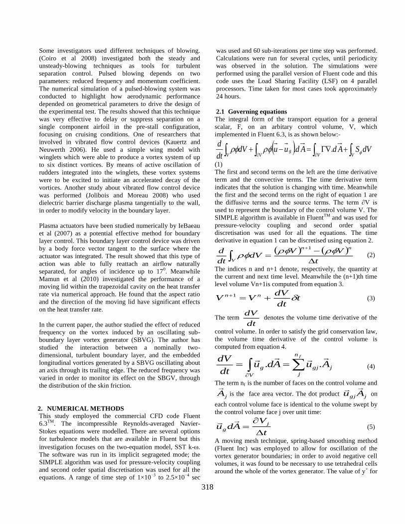
Figure 7 shows the contour of the normal anisotropy, -

22 '' u . One can see that the contours of -22 '' u

are characteristically cruciform, although about an axis on

the diagonal plane. The structures are almost symmetrical. The magnitudes in each of the lobes are almost equal and

opposite, with larger negative normal anisotropy magnitude

in the bottom right and the top left. The positive lobes lie on

a perpendicular plane to the latter. One can clearly see the

similarity of the four lobes either in the CFD or

experimental results, in the formation of a cruciform pattern.

The position of positive and negative lobes is also in the

same location as in the predicted data. These similarities

indicate that the prediction of 22 '' u is also reasonably

correct.

Figure 7 Comparison of Reynolds Shear Stress 222 /)(

Uw distribution at X1 (a) CFD (b)

Experiment

(a)

(b)

(a)

(b)

322

3.2 Embedded time dependent vortex/boundary layer

interaction

For time dependent flow, the SBVG was oscillated in a

range of reduced frequency of 4 to 10, from 0 to +15 degree

in simple harmonic motion. It is expected that the large eddy

frequency also falls into the same range; hence the selection

of the reduced frequency may stimulate a strong interaction

between the turbulent flow and the induced vortex. Figure 8

shows the contour of velocity magnitude on the cross-flow

plane at selected time steps. These figures were drawn such

that the viewer is looking downstream at the VG. The initial

state of the boundary layer and the wake can be seen at

time=0 sec. The wake of the VG is symmetric about the Y

axis. The first sign of vortex appearance is the asymmetry of

the velocity contour at = 5.33. As time progresses the

vortex continues to roll up and increases steadily until =

9.33. At this stage, the shape of the vortex core can be

observed clearly. It also can be observed that in the

common-flow down region, some thinning of the boundary

layer has taken place, due to the movement of the high-

momentum fluid drawn toward the wall. Meanwhile in the

common-flow up region, the low-momentum fluid is swept

upward causing a slight thickening of the boundary layer.

Due to this upward motion, a ’tongue’ structure appears in

the common-flow up region and rises out of the floor.

Figure 8 Contours of Velocity Magnitude at X1 location

3.3 Effects of reduced frequency

Skin friction plots have been drawn in order to show the

effects of the reduced frequency. Figure 9-11 show the

comparison of spanwise averaged skin friction between

static and oscillating SBVGs at various freestream locations

(X1, X2 and X3). From these figures, it can be observed that

there are three periods of time involved in the oscillating

SBVG history at these freestream locations. The first period

represents the flow condition before the arrival of the

induced vortex and this can be observed at the τ<5 for

location X1. This first period (also the second and third

periods) persists longer for X2, and X3 locations as they are

further downstream. The spanwise value of cf is constant

during this time period as nothing has yet happened to the

local flow.

Figure 9 Spanwise averaged of skin friction at X1

location

Figure 10 Spanwise averaged of skin friction at X2

location

The second period represents the initial interaction between

the induced vortex and the boundary layer. This can be

observed at 5< τ <15 for location X1. At the start of this

period, the spanwise averaged cf decreases momentarily due

to the arrival of the induced vortex at the measurement

location. By increasing the reduced frequency, this one-off

phenomenon becomes more apparent. The value of cf then

starts to increase until it reaches a peak value at which it

settles. Then, the flow enters upon its third period of time.

τ=0

τ=5.33

τ=6.67

τ=9.93

323

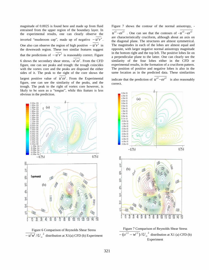
The most interesting feature is that increasing the reduced

frequency causes the final value of the spanwise averaged cf

to increase as well. For F+=10, the increment is about 2 %

of the static SBVG cf value. As Henry et al15

used the wall

shear to indicate beneficial effect of the SBVG therefore this

increment also indicates the positive effects of the

oscillating SBVG. It can also be observed that there is not

much difference in cf between F+=8 and F+=10.

Figure 11 Spanwise averaged of skin friction at X3

location

Figure 12 Time averaged of skin friction at X1 location

The trend of a beneficial cf increment however, does not

persist to location X3, as shown in Figure 11. From that

figure, it can be seen that the spanwise averaged cf for the

oscillating SBVG is below the static value. This

phenomenon may indicate that the momentum mixing

process decreases when the vortex moves downstream,

which may be due to the rapid diffusing of the vortex. It also

can be observed that the differences between cf for F+ = 4,

6, 8, and 10 persist for all streamwise locations. Figures 12-

14 show the time averaged cf after the flow has achieved

periodicity. It is noted that the plots in these figures were

drawn such that the viewer is looking downstream at the

SBVG.

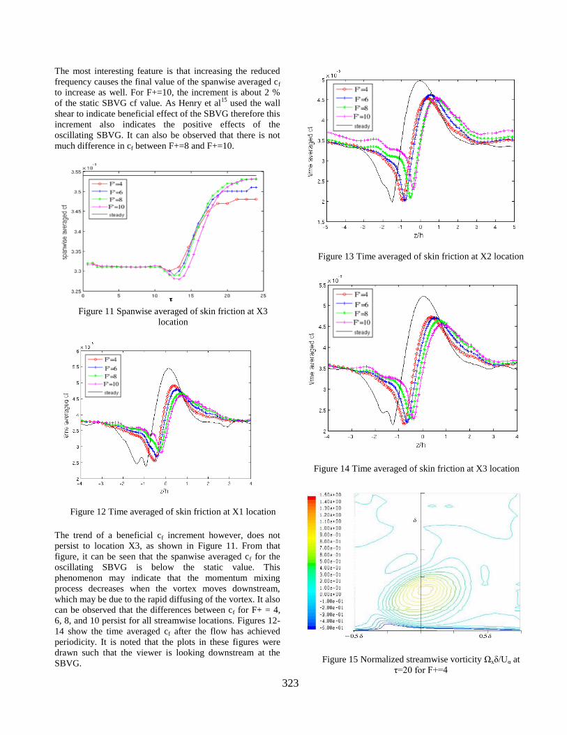
Figure 13 Time averaged of skin friction at X2 location

Figure 14 Time averaged of skin friction at X3 location

Figure 15 Normalized streamwise vorticity Ωxδ/Uα at

τ=20 for F+=4

324

Figure 16 Normalized streamwise vorticity Ωxδ/Uα at

τ=20 for F+=6

Figure 17 Normalized streamwise vorticity Ωxδ/Uα at

τ=20 for F+=8

Figure 18 Normalized streamwise vorticity Ωxδ/Uα at

τ=20 for F+=10

The first apparent remark is that the peak of the time

averaged cf for the oscillating SBVG is lower than the

static SBVG for all oscillating SBVG cases. This trend

continues up until the X3 location. The second remark is

that, the region influenced by the induced vortex is

shifted to the common-flow down region (to the right of

the domain). The shifting magnitude is directly

proportional to the reduced frequency and therefore an

increase in the value of reduced frequency also causes an

increase in the shifting magnitude.

Figure 19 Velocity vector in the X1 region at τ=20 for a)

F+=4 b) F+=10

Notice also that increasing the reduced frequency caused the

peak time averaged cf to decrease. Hence, the reduced

frequency is inversely proportional to the peak of time

averaged cf. Notice also that the distribution of cf is less

(a)

(b)

325

spread for the oscillating SBVGs. Although the spanwise

averaged cf for the oscillating SBVG is slightly higher than

the static SBVG, the static SBVG distribution of time

averaged cf involved greater extremes while the oscillating

SBVG elevated cf on both upwash and downwash sides.

This implies that the oscillating SBVG performance is better

than the static. It is also can be observed in the cf

distribution for static SBVG that a small bump appears at

z/h = -1. The bump may indicate that there is a sudden

change in the streamwise velocity gradient due to the effect

of fluid mixing. Figures 15-18 show contours of normalized

streamwise vorticity for F+=4, 6, 8, and 10 at τ=20. From

these figures, one can see an apparent elliptical structure,

which the author identifies as the primary vortex. By

increasing the reduced frequency to 10, the size of the

primary vortex increases, nearly 1.5 times of its size at

F+=4. The direction of the enlargement is toward the

common-flow down region, hence the vortex core also

moves toward this region. One also can see a weaker vortex

appear on the top left of the primary vortex, which the

author identifies as the secondary vortex. This secondary

vortex also increases in size when the reduced frequency is

increased. To clearly observe the motion of the fluid

particles, velocity vector plots are shown in Figure 19.

Figure 19(a) shows the velocity plots for the case of F+=4,

and it can be seen that the secondary vortex is not apparent

in this case. In contrast Figure 19(b) which was obtained

from the case of F+=10, the secondary vortex can clearly be

seen (on the top left of the primary vortex). The rotation of

the secondary vortex is in the anti-clockwise direction,

opposite to the direction of the primary vortex.

4. CONCLUSION

A numerical study of vortex generators in a low speed flow

has been completed. The comparison of Reynolds stresses

for static VG between experimental and prediction results

showed a satisfactory agreement. The increase in the

spanwise averaged skin friction with the increase in reduced

frequency is clearly observed. The time averaged skin

friction distribution for oscillating SBVG is less spread

compared to the static SBVG. The results also show that an

increase in the reduced frequency induces secondary vortex

to appear.

ACKNOWLEDGEMENT

The author would like to thanks Universiti Sains Malaysia

for sponsoring the work (RU Grant No. 814042).

REFERENCES

Gad-el-hak. 2001. Flow control: The Future, Journal of

Aircraft 3 (38):

Gad-el-hak. 2000. Flow Control Passive, Active, and

Reactive flow management, Cambridge Univ. Press,

London.

Collis, S.S., Joslin, R.D., Seifert, A. and Theofilis, V. 2004.

Issues in active flow control: theory,control, simulation

and experiment, Progress in Aerospace Sciences 40:237-

289

Lin, J.C. 2002. Review of research on low-profile vortex

generators to control boundary layer separation, Progress

in Aerospace Sciences 38: 389-420

Kupper, C. and Henry, F.S. 2003. Numerical study of air-jet

vortex generators in a turbulent boundary layer, Applied

Mathematical Modelling: 359-377

Ekaterinaris, J.A. 2004. Prediction of a active flow control

performance on airfoils and wings, Aerospace Science

and Technology 8: 401-410

Shojaefard, M.H., Noorpoor, A.R., Avanesians, A. and

Ghaffarpour, M. 2005. Numerical Investigation of Flow

Control by Suction and Injection on a Subsonic Airfoil,

American Journal of Applied Sciences: 1474-1480

Coiro, D.P., Bellobuono, E. F. and Nicolos, F. 2008.

Improving aircraft endurance through turbulent

separation control by pulsed blowing, Journal of Aircraft,

3(45):

Guo, Y. 2008. Acoustic analysis of low-noise actuator

design for active flow control, Journal of sound and

Vibration :843-860

Kauertz, S. and Neuwerth. G. 2006. Excitation of

instabilities in the wake of an airfoil by means of active

winglets, Aerospace Science and Technology 10: 551-

562

Jolibois, J. and Moreau, M.F.E. 2008. Application of an AC

barrier discharge actuator to control airflow separation

above a NACA 0015 airfoil: Optimization of the

actuation location along the chord, Journal of

Electrostatic: 495-503

IeBeau, R.P., Reasor, D.A., Suzen, Y.B., Jacob, J.D. and

Huang, P.G. 2007. Unstructured Grid simulation of flow

separation control using plasma actuators,18th

AIAA

Computational Fluid Dynamics Conference, Florida

Benard, N., Jolibois, J. and Moreau, E. 2009. Lift and drag

performances of an axisymmetric airfoil controlled by

plasma actuator Journal of Electrostatic: 1-7

Martin, L. 2001. Experimental and Computational

Investigtaion of Sub-Boundary Layer Vortex Generators,

PhD Dissertation, Queen’s University of Belfast,

Northern Ireland

Pearcey, H.H. and Henry, F.S. 1994. Numerical model of

boundary layer control using air jet generated vortices,

AIAA Journal, 32 (12):

ANSYS FLUENT User’s Guide

Mamun, M.A.H., Tanim, T.R., Rahman, M.M., Saidur, R.

and Nagata, S. 2010. Mixed Convection Analysis in

Trapezoidal Cavity with a Moving Lid, International

Journal of Mechanical and Materials Engineering 5(1):

18-28