The 2012 World Congress on Advances in Civil, Environmental, and Materials Research (ACEM’ 12)Seoul, Korea, August 26-30, 2012

Numerical Study of Influence of Ice Location on Galloping of an Iced Conductor

*A. Borna1), W.G. Habashi2) and G. McClure3)

1), 2) Computational Fluid Dynamics Laboratory, Department of Mechanical Engineering 3) Department of Civil Engineering and Applied Mechanics

McGill University, Montreal, QC, Canada

ABSTRACT

In the field of overhead transmission lines, galloping is of immediate concern due to its impact over the mechanical reliability and serviceability of electrical power networks. It is known that smooth circular cylinders are immune to gallop and there are only few galloping cases on bare conductors reported in the literature. Hence, galloping of transmission lines are usually accompanied by ice accretion. Although ice accretion over conductors is required for a galloping event, not all ice profiles lead to instability. Several icing parameters including the amount of ice accretion, shape of the ice profile, and the initial location (orientation) of the ice over a conductor combine to cause a galloping event. In this paper, the effects of initial orientation of the ice on flow-induced instabilities of an iced conductor are studied by employing an aeroelastic numerical approach. The numerical approach is a two-way loosely coupled fluid-structure interaction consisting of three key modules: Computational Fluid Dynamics (CFD), Computational Structural Dynamics (CSD), and communication and data-handling module. A smooth, glaze iced profile with maximum ice thickness of 37% of the conductor’s diameter is considered at various initial orientations over the conductor to study the risk of galloping at different ice orientations. Moreover, the numerical results are compared with the Den Hartog instability criterion in order to assess the possibility of galloping outside the Den Hartog region.

1. INTRODUCTION

Overhead transmission line conductors are flexible structures subject to unsteady wind-induced loading and consequent motion. The dynamic characteristics of such motion, namely its frequency and amplitude, are directly related to the magnitude and frequency content of the wind loading and the structural dynamic characteristics of the transmission line. Wind-induced motions can be classified into three general categories : 1) very small amplitude and high frequency (Aeolian vibrations), 2) small amplitude and moderate frequency, recognized as wake- and vortex-induced oscillations, and, finally, 3) a self-sustained, high-amplitude, and low frequency flutter instability known as galloping (Blevins 1994, EPRI 2006, Lilien et al. 2007, Païdoussis                                                             1) Ph.D. Candidate: amir.borna@mail.mcgill.ca 2) Professor and Director 3) Associate Professor 

et al. 2011). These three categories of conductor motion are also distinguished by other factors such as energy transfer mechanism, type of motion, and different forms of damage they may induce to transmission line components. For example, Aeolian vibrations and wake-induced oscillations have moderate to high frequency low-amplitude characteristics that may cause wear and fatigue of conductor components, while larger galloping motion, in addition, may cause flashover between adjacent phases, which may lead to power outage and direct cable damage, cable tension increase and dynamic loading on the supporting towers and connecting hardware, and, in extreme situations, cable rupture, structural damage, and tower failure. Severe cases, such as tower failure and blackouts, may occur during winter and in remote areas, complicating the repair process. These damages and other impacts of transmission line vibrations on the reliability and serviceability of electrical power networks are well studied in the literature (e.g. see (EPRI 2006, Lilien et al. 2007)). Each year, millions of dollars are spent worldwide to repair such damages and/or overcome the cost of subsequent economical impact. Hence, wind-induced motions of conductors, and in particular galloping, are an important consideration in designing transmission lines, especially in geographical regions prone to atmospheric icing.

The character of instability in galloping is velocity-dependent and damping-controlled (Païdoussis et al. 2011). It means that during a galloping event, a bluff body receives energy supplied by wind, and the effective damping present in the mechanical line system plays an important role in decreasing or increasing the amplitude of displacements. Effective damping combines both structural and aerodynamic damping energy dissipation phenomena, and in order to have an oscillatory instability, it is required to have a negative effective damping where energy is absorbed by the system rather than dissipated.

Normally, in the case of bare conductors, wind loading, damping, and inertia forces do not impose large motions in the vertical direction when subject to horizontal incident wind, but the aerodynamic conditions of the conductor change dramatically in the presence of atmospheric icing accretions (Lilien et al. 2007). In fact, it is shown that bare smooth-surface cylinders are practically immune to very large amplitude, galloping-type oscillations (Païdoussis et al. 2011), and there are only few galloping cases on bare overhead line conductors reported in the literature (Farzaneh 2008). Therefore, in almost all of the observed conductor galloping events, ice accretion and threshold wind speed combinations are present. Moreover, the orientation of the ice deposit with respect to incident wind, the iced conductor profile, and the magnitude of the incident wind velocity are combined parameters that influence the likelihood of galloping, although it is difficult to assign a confidence level to such predictions. In this paper, the effects of the ice orientation and magnitude of the incident wind velocity on overhead conductor galloping are studied using a computational aeroelastic approach through a number of test cases.

2. NUMERICAL AEROELASTIC APPROACH

Current methods to predict galloping fail in many practical cases, mainly due to their inherent limitations and simplifications. On the one hand, full-scale experimental set-ups are expensive, and such tests are compromised by the difficulty to replicate

realistic natural icing conditions as not all weather conditions and ice deposit profiles can be simulated by icing tunnels or natural icing experiments. On the other hand, computational methods for predicting and preventing conductor galloping through unsteady flow calculation become of great interest. Computational aeroelastic analysis dispenses with the common quasi-steady assumption, and makes it possible to capture the time-accurate response of the structure under different ambient air flow conditions. In addition, the analysis can simulate different natural conditions and ice profiles that are non-uniform along the span, which are more realistic and therefore contribute to the added credibility and acceptability of the numerical aeroelastic approach.

2.1. Fluid Dynamics The unsteady Reynolds-Averaged Navier-Stokes (URANS) equations are solved

using FENSAP-ICE, a second order time accurate, 3D finite element compressible Navier-Stokes solver (Habashi et al. 2004, Habashi 2009). The Arbitrary Lagrangian Eulerian (ALE) formulation of the Navier-Stokes equations is applied to compute the time-accurate solution of the flow field with moving meshes. The non-dimensional ALE formulation of URANS equations used in FENSAP-ICE can be expressed as follows:

( ), ,0 ,i i i i

u utρ ρ ρ∂− + =

∂ (1)

( ) ( ) ( )1, ,, , ,

Re ,ii i i j i ij j i ji j j

u u u u u p u utρ ρ ρ τ ρ−

∞

∂− + = − + −

∂ (2)

where ρ is air density, t , time, iu , the ith component of velocity, ,iu mesh velocity, p , pressure, τ , stress tensor, Re∞ , free-stream Reynolds number, and i ju u is the Reynolds stress tensor. Eq. (1) holds for the conservation of mass equation, and Eq. (2) shows the conservation of momentum (Navier-Stokes) equations. These equations suffer from a closure problem, i.e. Reynolds stress tensor needs to be computed. Various turbulent-viscosity models, such as algebraic, one-equation, two-equation, Reynolds-stress and higher order models are developed (see e.g. (Pope 2000)) to solve the closure problem. In theory, accuracy increases with the level of turbulence model, but the computational cost and simplicity of coding are important factors in unsteady applications. Hence, the turbulent-viscosity model is chosen as follows,

223i j t ij iju u S kν δ= − + (3)

In this equation, the local mean rate of strain, ijS , is calculated using the mean flow

velocities, and the eddy viscosity, tν , and the turbulent kinetic energy, k , are estimated from the one-equation Spalart-Allmaras model (Bardina 1997).

Finally, it should be noted that at each time step, a Laplace equation is solved in order to handle the moving nodes on the fluid/structure boundary and determine the new equilibrium position and velocity of the internal nodes, i.e. the mesh velocity, iu , of the fluid domain. This mesh velocity field is used in Eq.(2).

2.2. Equations of Motion The incremental equations of motion of a structure idealized as a linear multi-

degree-of-freedom system can be expressed in the form of Eq. (4).

{ } { } { } { }M q C q K q F⎡ ⎤ ⎡ ⎤ ⎡ ⎤⎣ ⎦ ⎣ ⎦ ⎣ ⎦∆ + ∆ + ∆ = ∆ (4) In this equation, [M] is the mass/inertia matrix, [C], the structural viscous damping

matrix, and [K], the stiffness matrix. For the problem at hand {q} ≡ (x, y, θ)T is the displacement vector measured from the initial static equilibrium and {F} is the external dynamic fluid loading vector resulting from the conductor surface loading. The dot operator holds for the time derivative, and the ∆ is the forward difference operator in time. The equations of motion are solved in full-space by direct time-step integration using the second order unconditionally stable Newmark-Beta operator (Bathe 2006).

2.3. Coupling Algorithm A two-way loosely coupled approach is applied in which the fluid and solid equations

are successively and separately solved (with independent solvers) using non-matching grids. Then, the latest information provided by each part of the coupled system is called by the other part in order to proceed in time. The coupling algorithm includes three main modules: the fluid dynamics solver, the solid structural dynamics solver, and the load/motion transfer operator that relays relevant analysis parameters between the two solution domains. The solution process starts with an initial flow field that provides the surface fluid tractions along the fluid/structure mesh interface. Next, using the conservative load transfer operator, surface tractions are integrated to yield the resultant nodal forces to be applied as external loads on the solid mesh. The solution of Eq. (4) provides the displacement, velocity and acceleration vectors of the solid mesh nodes at every time step. After each time increment, the conductor displacements are imposed via the compatibility condition to the nodes of the fluid mesh along the fluid/structure interface. Then, the flow solver introduces this interface motion in the fluid flow formulation to compute the fluid mesh motion in the entire domain, and then solves the flow field. This loop proceeds in time until the total analysis duration is achieved.

 2.4. Model and Parameters In order to study the effect of the initial ice deposit orientation with respect to incident

wind flow on conductor galloping, a symmetric glaze iced conductor with maximum ice thickness of 37% of the conductor diameter is considered at different initial orientations (ϕ ) relative to the incident wind. Fig. 1 illustrates the geometry of the model, the flow boundary conditions, while the top right insert shows the profile of the iced conductor and defines the angle ϕ . The incident wind velocity range of 10-30 m/s is considered. The natural frequencies of translational galloping oscillations of the iced conductor on flexible supports, representing the mid span oscillations of a typical high voltage line

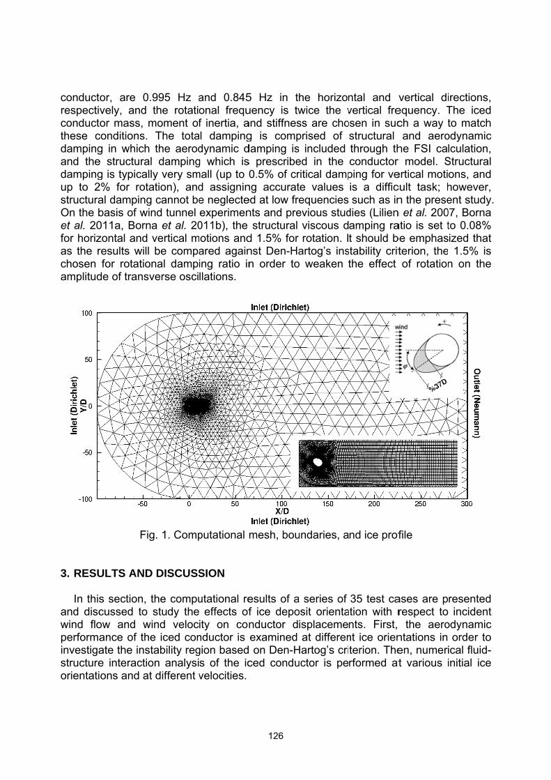
conductrespectivconductthese cdampingand thedampingup to 2structuraOn the bet al. 20for horizas the rchosen amplitud

3. RESU

In thisand discwind floperformainvestigastructureorientati

or, are 0vely, and or mass, m

conditions. g in whiche structurag is typical2% for rotaal dampingbasis of wi011a, Bornzontal and results willfor rotatio

de of transv

Fig

ULTS AND

s section, cussed to ow and wance of thate the inse interactioons and at

.995 Hz athe rotatio

moment ofThe tota

the aerodl dampingly very smation), andg cannot bend tunnel

na et al. 20vertical m be compa

onal dampiverse osci

g. 1. Comp

D DISCUSS

the compustudy the

wind veloce iced con

stability regon analysit different v

and 0.845onal frequf inertia, al dampingdynamic dg which ismall (up to 0d assignine neglecteexperimen011b), the otions andared againing ratio inllations.

putational m

SION

utational reeffects of

ity on connductor is gion baseds of the icvelocities.

5 Hz in tuency is twand stiffnesg is compdamping iss prescribe0.5% of cr

ng accurated at low frents and pre

structural d 1.5% for nst Den-Han order to

mesh, bou

esults of af ice deponductor dexamined on Den-Hced condu

he horizonwice the vss are choprised of s included ed in the ritical dampte valuesequenciesevious stud

viscous drotation. I

artog’s inso weaken t

undaries, a

a series of osit orientaisplacemeat differen

Hartog’s criuctor is pe

ntal and vvertical fre

osen in sucstructural through thconductor ping for veis a difficsuch as in

dies (Lilienamping rat should b

stability critthe effect

nd ice prof

35 test caation with rnts. First, nt ice orienterion. Therformed at

vertical diequency. Tch a way tand aero

he FSI car model. Sertical moticult task; hn the prese

n et al. 200atio is set tbe emphasterion, theof rotation

file

ases are prespect to

the aerontations in en, numerit various i

irections, The iced to match

odynamic lculation,

Structural ons, and however, ent study.

07, Borna to 0.08% ized that 1.5% is n on the

resented incident

odynamic order to

ical fluid-initial ice

3.1. D The f

Den Hacoefficiepredict asystem. when thbecome

In ordthe unstunsteadvortex paerodynaerodyndeposit figure. Binstabilitcriterionand is awords, tzone.

Fig. 2

3.2. A In the

unstead

Den-Hartog

first explanartog (Deents and tha negativeDen Harto

he rate of cs negative

der to numteady flowy loading patterns bnamic coenamic coefforientationBased on ty only at a, due to its poor pred

there migh

2. Comput

Aeroelastic

e case of hy loading

g instability

nation for gn-Hartog heir gradiee effective og’s criteriochange of

e and exceerically inv

w field aroover the b

behind the fficients aficients of

n are plotteDen-Harto

a very sms simplicitydictor of inst be other

tational tim

instability

eavily sepand aerod

y zone

galloping a1932). He

ent with resdamping

on states tthe lift co

eds the dravestigate thund the p

body is combody are

are calculathe non-m

ed; the derog’s gallopall area ar

y, can only stability liminstability

me-average

zone

arated flowynamic da

as an aerode proposespect to thcondition that a bod

oefficient (ag coefficihis criterioprofile at vmputed. Te fully devated. In F

moving (fixerivative of tping criterround 180o

describe amits of a m

conditions

ed aerodynorientation

w over blufamping are

dynamic med a relahe angle othat wouldy is prone

lC ) with reent ( dC ), tn for the stvarious ori

The calculaveloped aFig. 2, thed) iced cothe lift coefrion, the ico (see Figa small poulti-degrees outside o

namic coeffn

ff bodies, se functions

mechanismation betwof attack (αd cause th

to gallop iespect to that is whetudied icedentations

ations are nd then te comput

onductor vefficient is aced condu. 2), whichrtion of the

e-of-freedoof the Den-

ficients ver

such as thes of both th

m was presween aeroα ϕ≡ − ) in

he instabiliin vertical the angle

en ldC dα +d conductois solved continued

the time ated time-aersus the also incluductor is suh confirms e instability

om system.-Hartog’s i

rsus ice de

e present che incident

ented by odynamic

order to ty of the direction of attack

0dC < . or profile,

and the until the

averaged averaged initial ice ed in the ubject to that this

y domain . In other nstability

eposit

case, the t velocity

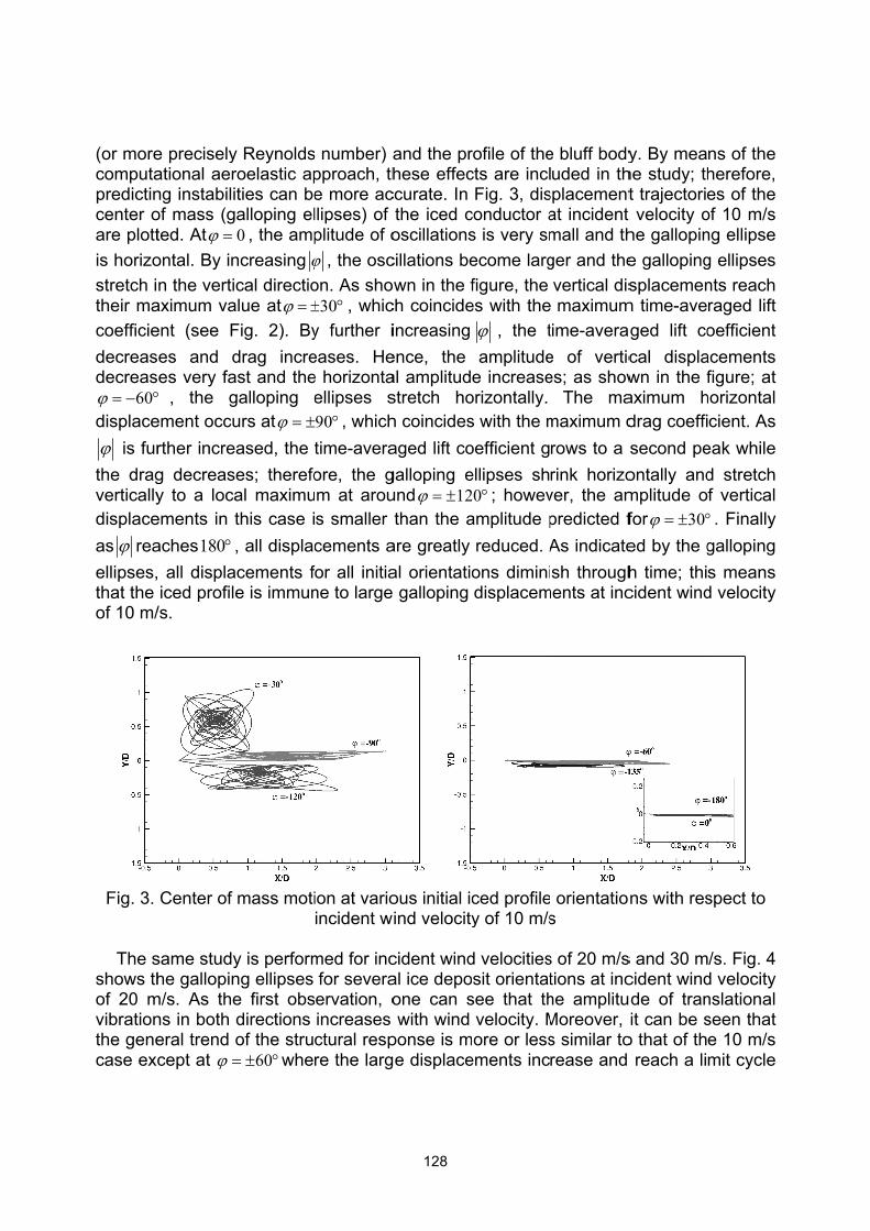
(or morecomputapredictincenter oare plottis horizostretch itheir macoefficiedecreasdecreas

60ϕ = − °displaceϕ is furthe dragverticallydisplaceas ϕ reaellipses,that the of 10 m/

Fig. 3.

The s

shows thof 20 mvibrationthe genecase exc

e preciselyational aerng instabiliof mass (gted. Atϕ =ontal. By inn the vertic

aximum vaent (see Fes and des very fa° , the gement occurther increg decreasey to a locaements in taches180° , all displaiced profile

/s.

Center of

same studyhe gallopin

m/s. As thens in both eral trend ocept at ϕ =

y Reynoldsroelastic apties can bealloping el0 , the amp

ncreasing ϕcal directio

alue atϕ = ±Fig. 2). Bydrag increast and thegalloping eurs atϕ = ±

ased, the es; therefoal maximuthis case i, all displaccements fe is immun

mass moti

y is performng ellipses e first obsdirections of the stru

60= ± °whe

s number) approach, the more acllipses) of plitude of oϕ , the oscon. As show

30± ° , whicy further ieases. Hee horizontaellipses s90° , whichtime-averaore, the gm at arous smaller cements afor all initiane to large

ion at varioincident w

med for incfor severaervation, oincreases ctural respre the larg

and the prhese effec

ccurate. Inthe iced coscillationscillations bewn in the f

ch coincideincreasing

ence, the al amplitudstretch hoh coincidesaged lift cogalloping eund 12ϕ = ±than the a

are greatly al orientatio galloping

ous initial icind velocity

cident windal ice depoone can swith wind

ponse is me displace

rofile of thects are inclFig. 3, dis

conductor as is very smecome largfigure, the

es with theϕ , the tamplitude

e increaseorizontally. s with the moefficient gellipses sh20° ; howevamplitude preduced. Aons diminidisplacem

ced profiley of 10 m/s

d velocitiessit orientat

see that thvelocity. More or less

ements inc

e bluff bodyuded in th

splacementat incident mall and thger and thevertical dis maximumtime-averae of vertices; as show

The mamaximum drows to a rink horizo

ver, the ampredicted fAs indicatesh through

ments at inc

orientatios

s of 20 m/stions at inche amplituMoreover, s similar torease and

y. By meahe study; tht trajectoriet velocity ohe gallopine gallopingsplacemen

m time-aveged lift cocal displawn in the faximum hdrag coeffisecond peontally andmplitude ofor 30ϕ = ± °

ed by the gh time; thicident wind

ns with res

s and 30 mcident windde of tranit can be s

o that of threach a li

ns of the herefore, es of the

of 10 m/s ng ellipse g ellipses nts reach raged lift oefficient

acements figure; at

horizontal cient. As

eak while d stretch f vertical ° . Finally galloping s means d velocity

spect to

/s. Fig. 4 d velocity nslational seen that e 10 m/s mit cycle

(see alsand its mThe instcriterion

Fig. 4.

In Fig

velocity translatishows this signifpresent.quickly negativeincreasinthe verthoweverpeak-to-from thesimilar thorizont

180ϕ =increaseaveragevortex-inand the It shouldsame amoscillatioinstabilit

o Fig. 7). Tmagnitude tability of t.

Center of

g. 5, the gaof 30 m/

onal vibrahe velocityficantly diff. As shownexcept fo

e aerodynng the liketically reclr, the verti-peak ampe lower ino the 20 mtal amplitu, the hor

e with a veed lift coeffinduced vibamplitude

d be notedmount of ons are noty can be s

This indicais larger t

his particu

mass moti

alloping el/s are shotions in bo

y-dependenferent fromn in the figor the follamic damelihood of ined ellipsical displacplitude amcident win

m/s; i.e. thede at limitizontal os

ery small raicient (see

brations in at limit cyc

d that althophysical tiot reachedseen well a

ates that fohan the valar iced pr

ion at varioincident w

lipses for own. Simioth directioncy of the

m the prevure, the osowing reg

mping at tlarge amp

se in Fig. cements inong all ot

nd velocitiee oscillatiot cycle is tcillations date. The sFig. 2). Thwhich the cle is expeough the ame for alld a limit cat the relev

or 60ϕ = ± °alue of strurofile orien

ous initial icind velocity

several icelar to theons increadisplacem

vious two scillationsgions: ϕ =these regiplitude ins5, the ho

ncrease anther test ces. In the ons reach the highesdamp quicmall ampliherefore, th oscillation

ected to beaeroelastic test case

cycle. Thisvant phase

, the aeroductural damtation is no

ced profiley of 20 m/s

e deposit oe 20 m/s ases with

ments; howcases andat differen

30, 60,± ±ions prevatabilities. A

orizontal ond reach a

cases. Thiscase ofϕ

a limit cycst among ockly, whileitude increhe instabilns are caue in the ordc computates, only ins response plot in Fig

dynamic damping assigot predicte

orientatios

orientationcase, the incident wever, the s

d more unt initial ice 180 . Thisails the stAt 30ϕ = ±

oscillations a limit cycs response

60ϕ = ± , thcle in whichother oriene the vertiase rate isity for 1ϕ =sed due toer of the ctions are a

the lattere and the g. 6.

amping is gned in th

ed by Den-

ns with res

ns for incid amplitude

wind velocistructural rstable reg

e orientatios shows tructural d, as illustdecrease

le with thee is quite he oscillath the peakntations. Fical displas due to ze180 can bo load fluc

conductor daccomplishr case, the

slow pac

negative e model. -Hartog’s

spect to

ent wind e of the ity which response gions are ns damp that the

damping, trated by e rapidly; e highest

different tions are k-to-peak Finally, at acements ero time-e type of

ctuations, diameter. hed for a e vertical ce of the

Fig. 5.

Phaseillustratioany potedisplacedisplacewind ve

180ϕ =there is the phadisplacestable li

30ϕ = −while at

Fig. 6. P

Center of

e plots, raons to studential limit

ements, i.eements areelocities. F. As showno stable

ase plot sements deimit cycle , see Fig.30 m/s, di

Phase plot

mass mot

ate of chady responst cycles. Ine. the trane providedFig. 6 reprn, the amplimit cycle

shows thaecrease ra

for both i. 8, we casplacemen

of transve

tion at varioincident w

nge of a se of a sysn the follonsverse ve at select resents thplitude of th

for the dut the oscpidly. Theincident w

an see thants converg

erse displac20 m

ous initial iind velocity

variable vstem and

owing figurelocity of t

ice oriente phase he oscillatiuration of tcillations se phase pwind velociat at 20 m/ge to a larg

cements am/s and 30

ced profiley of 30 m/s

versus the analyze thres, the phthe oscillaations for plots for tions increahe computlow down

plots for ϕties. By /s the oscge amplitu

t 180ϕ = f0 m/s

e orientatios

variable ihe instabilithase plotsations vers

20 m/s antransverse ases gradutations. Ho and the

60= − (Fiinvestigati

cillations dade limit cy

for inciden

ons with res

itself, are ties and d

s of the trasus the trand 30 m/s displacem

ually for 30owever, for

amplitudeg. 7) conng phase amp out v

ycle.

nt wind velo

spect to

practical etermine ansverse ansverse incident ments at 0 m/s, yet r 20 m/s, e of the firm one plots at

very fast,

ocities of

Fig. 7. P

 

Fig. 8.

4. CONC Comp

orientatiand thecriterionaround ϕparticulaof 30 maverageoscillatio

Moreoorientatilarge am

Phase plot

Phase plo

CLUDING

putational ons at thr

e results a. The De

180ϕ = ± °ar orientatim/s, the coed lift at ϕ =on. over, aeroon for inci

mplitude li

of transve

ot of transv

REMARK

aeroelasticee incidenare compn-Hartog’swhile the on at incidomputation

180= ± ° , th

oelastic coident wind mit cycle

rse displac20 m

verse displaof 20

KS

c instabilitnt wind velared with

s instabilityaeroelas

dent wind vns reveal his instabili

omputationvelocity o

oscillation

cements atm/s and 30

acementsm/s and 3

ty of an iclocities of

the predy analysisstic compuvelocities oa slowly gity is not e

ns show of 10 m/s.

is observ

t 60ϕ = −0 m/s

at 30ϕ = −30 m/s

ced conduc10 m/s, 20

dictions us shows outations sof 10 and growing inxpected to

that thereFor incide

ved at ϕ =

for inciden

for incide

ctor with v0 m/s andsing Den-Honly a smahow no 20 m/s. Ho

nstability. Do end up to

e is no unt wind ve

60± ° , and

nt wind velo

ent wind ve

various iced 30 m/s isHartog’s iall instabilinstability owever, atDue to zeo a large a

unstable inelocity of 2d for 30 m

ocities of

elocities

ed profile s studied nstability lity zone for this

t velocity ero time-amplitude

nitial ice 20 m/s, a m/s case,

unstable zones at 60ϕ = ± ° and 30± ° are detected, which are not predicted by Den-Hartog’s model.

In summary, the results show the failure of the Den-Hartog’s aerodynamic criterion to predict all potential instability zones and provide evidences that galloping instability is a velocity-dependent and damping-controlled, namely controlled by aerodynamic damping. Hence, accurately predicting the likelihood of galloping instabilities requires an aeroelastic approach.

REFERENCE Bardina, J.E., Huang, P. G., Coakley, T. J. (1997), Turbulence modeling validation,

testing, and development, National Aeronautics and Space Administration, Ames Research Center; National Technical Information Service, Moffett Field, CA.

Bathe, K.-J. (2006), Finite Element Procedures, Cambridge. Blevins, R.D. (1994), Flow-induced vibration, Krieger, Malabar, Florida. Borna, A., Habashi, W.G., McClure, G. and Nadarajah, S. (2011a). "Numerical

Modeling of Ice Accretion Effects on Galloping of Transmission Line Conductors". 9th International Symposium on Cable Dynamics, Shanghai, China, October 18-20 2011.

Borna, A., Habashi, W.G., Nadarajah, S.K. and McClure, G. (2011b), A Computational Aeroelastic Approach to Predict Galloping of Iced Conductors with 3 Degrees of Freedom, Chongqing University, China.

Den-Hartog, J.P. (1932), "Transmission Line Vibration Due to Sleet", Transactions of the American Institute of Electrical Engineers. 51(4), 1074-1076.

EPRI (2006), EPRI Transmission line reference book: Wind-induced conductor motion, Electric Power Research Institute, Palo Alto, CA: 2006. 1012317.

Farzaneh, M. (2008), Atmospheric icing of power networks, Springer, Dordrecht, London.

Habashi, W.G. (2009), "Advances in CFD for in-flight icing simulation", Journal of Japan Society of Fluid Mechanics. 28(2), 99-118.

Habashi, W.G., Aubé, M., Baruzzi, G., Morency, F., Tran, P. and Narramore, J.C. (2004), FENSAP-ICE: A full-3d in-flight icing simulation system for aircraft, rotorcraft and UAVS, Yokohama, Japan

Lilien, J.-L., Van Dyke, P., Asselin, J.-M., Farzaneh, M., Halsan, K., Havard, D., Hearnshaw, D., Laneville, A., Mito, M., Rawlins, C.B., St-Louis, M., Sunkle, D. and Vinogradov, A. (2007), Task Force B2.11.06, State of the art of conductor galloping, Technical Brochure 322. CIGRÉ (International Council of Large Electrical Networks), Scientifc Committee B2 on Overhead Lines.

Païdoussis, M.P., Price, S.J. and de Langre, E. (2011), Fluid-Structure Interactions - Cross-Flow-Induced Instabilities, Cambridge University Press

Pope, S.B. (2000), Turbulent flows, Cambridge University Press, Cambridge ; New York.