numerical study of helical pipe flow

Tit

le:

Nu

mer

ical

Stu

dy o

f H

elic

al P

ipe

Flo

w

S

epte

mb

er, 2

017

A

nu

p K

um

er D

atta

Numerical Study of Helical Pipe Flow

Ph.D Thesis

September, 2017

Anup Kumer Datta

The Graduate School of Natural Science and Technology

(Doctor Course)

OKAYAMA UNIVERSITY, JAPAN

Numerical Study of Helical Pipe Flow

A thesis

Submitted in partial fulfillment of the requirements for the degree of

Doctor of Philosophy

by

Anup Kumer Datta

Under the supervision of

Professor Shinichiro YANASE

The Graduate School of Natural Science and Technology

(Doctor Course)

Okayama University, Japan

September, 2017

Dedication

This dissertation is dedicated to my late father who shaped part of my

vision and taught me the good things that really matter in life

Anup Kumer Datta

September, 2017

i

Contents

Abstract…………………………………………………………………………… 1

Acknowledgement………………………………………………………………… 3

List of Figures…………………………………………………………………….. 4

List of Tables……………………………………………………………………… 10

Nomenclature……………………………………………………………………... 11

Dissertation contents……………………………………………………………… 13

Chapter 1 Introduction……………………………………………………. 16

1.1 Definition of some useful parameters…………………….. 17

1.2 Flow in curved pipes………………………………………. 19

1.3 Flow in helical pipes………………………………………. 21

1.3.1 Non-orthogonal coordinate system…………………. 23

1.3.2 Orthogonal coordinate system………………………. 24

1.4 Flow pattern through curved and helical pipes……………. 28

1.5 Influence of pitch on the flow pattern……………………… 32

1.6 Stability of the flow in a helical pipe……………………… 33

1.7 Pressure drop and friction factor………………………….. 36

1.8 Heat transfer of flow through curved and helical pipes…… 39

Chapter 2 Mathematical formulation…………………………………….. 51

2.1 Mathematical formulation and governing equations……… 51

2.2 Turbulence models………………………………………… 54

2.2.1 RNG 𝑘 − 휀 model…………………………………. 55

2.2.2 Lien-cubic 𝑘 − 휀 model…………………………… 56

2.2.3 Launder-Sharma 𝑘 − 휀 model……………………... 57

2.3 Boundary conditions………………………………………. 58

Chapter 3 Numerical methods……………………………………………. 59

3.1 Numerical methods………………………………………... 59

3.2 Finite volume discretization………………………………. 59

3.2.1 Discretization of the solution domain……………… 60

ii

3.3 Discretization of the transport equation…………………… 62

3.3.1 Discretization of spatial terms……………………… 64

3.3.1.1 Convection term………………………….. 65

3.3.1.2 Convection differencing scheme………….. 66

3.3.1.3 Diffusion term…………………………….. 68

3.3.1.4 Source term……………………………….. 69

3.4 Temporal discretization …………………………………… 70

3.5 Solution techniques………………………………………... 73

3.6 Discretization procedure for the Navier-Stokes system……. 76

3.6.1 Derivation of the pressure equation………………… 78

3.6.2 Pressure-velocity coupling…………………………. 79

3.6.2.1 The PISO algorithm for transient flows…… 79

3.6.2.2 The SIMPLE algorithm…………………… 80

3.6.3 Solution procedure for the Navier Stokes equation… 82

Chapter 4 Laminar flow through a helical pipe with circular cross

section…………………………………………………………...

85

4.1 Objectives and scope of this chapter………………………. 84

4.2 Results……………………………………………………... 86

4.2.1 Two dimensional steady state and the definition of

Re and Dn………………………………………….

86

4.2.2 Dean number calculated in the present study……… 89

4.2.3 Secondary flow for 𝛿 = 0.4……………………….. 90

4.2.4 Axial flow for 𝛿 = 0.4……………………………... 92

4.2.5 Flux through the pipe………………………………. 94

4.3 Unsteady solutions………………………………………… 95

4.3.1 Method to obtain the critical Reynolds number……. 95

4.3.2 Critical Reynolds number for various 𝛽…………… 97

4.3.3 Time evolution of the equi-surface of the axial flow

velocity …………………………………………….

99

4.4 Discussion and conclusion………………………………… 105

Chapter 5 Effect of torsion on the friction factor of helical pipe flow….. 107

iii

5.1 Objectives and scope of this chapter……………………….. 107

5.2 Results…………………………………………………….. 108

5.2.1 Comparison with the experimental data for Type -1 110

5.3 Axial flow distribution for Type -1……………………….. 114

5.4 Friction factor over a wide range of 𝛽…………………….. 116

5.4.1 Friction factor for Type -1 (𝛿 = 0.1)……………….. 116

5.4.2 Friction factor for Type -2 (𝛿 = 0.05)………………. 119


Chapter 6 Thermal flow through a helical pipe with circular cross

section…………………………………………………………...

124


6.2 Results……………………………………………………... 125

7.2.1 Nusselt number…………………………………….. 126

6.3 Torsion effect on the Nusselt number……………………… 127

6.4 Torsion effect on the secondary flow and temperature field.. 129

6.5 Local Nusselt number……………………………………… 133


Chapter 7 Turbulent flow through a helical pipe with circular cross

section…………………………………………………………...

136


7.2 Results……………………………………………………... 138

7.3 Results of the case for 𝛽 = 0.02…………………………… 140

7.4 Results of the case for 𝛽 = 0.45…………………………… 148


Chapter 8 General conclusions…………………………………………… 158

References ………………………………………………………… 162

1

Abstract

Flows and heat transfer in helical pipes have attracted considerable attention not only because

of their ample applications in chemical, mechanical, civil, nuclear and biomechanical

engineering but also their physical interest of secondary flow patterns and soon. In this

dissertation, three dimension (3D) direct numerical simulations (DNS) of viscous

incompressible isothermal (without heat transfer) and thermal (with heat transfer) laminar

and turbulent fluid flows through a helical pipe with circular cross section are presented,

where the wall of a helical pipe is heated for thermal case. Note that the case of turbulent

flow through a helical pipe, we also used three different turbulent models based on the

Reynold averaged Navier-Stokes equation (RANS). Numerical calculation were carried out

over a wide range of Dean number, Dn, curvature, 𝛿 , torsion parameter, 𝛽 , the Prandtl

number, Pr, and the Reynolds number, Re, for both the laminar and turbulent flow cases.

OpenFOAM was used as a tool for the numerical approach. To generate a suitable mesh in

the flow domain, an appropriate mesh system with 3D orthogonal helical coordinates was

successfully created to conduct accurate DNSs and turbulence models of helical pipe flow

using an FVM-based open-source computational fluid dynamics package (OpenFOAM).

First, the laminar flow in a helical pipe with circular cross section was investigated. The

instability of the steady solutions of the helical pipe flow was studied instead of the linear

stability analysis. We found the neutral curve of the critical Reynolds numbers of the laminar

to turbulent transition by observing unsteady behaviors of the solution. The present results of

the critical Reynolds number nearly agree with the two-dimensional (2D) linear stability

analysis (Yamamoto et al. (1998)) except for the lowest critical Reynolds number region,

where the present study gave the critical Reynolds numbers much less than those by the 2D

linear stability analysis and showed explosive 3D instability occurred slightly in the marginal

instability state. It is interesting that we found a close relationship between the disturbances

of unsteady solutions (such as nearly 2D state, nonlocal 3D modification, highly nonlinear

behaviours, continuous nonperiodic oscilation), and the vortical structure of steady solutions

in helical pipe flow.

2

Then, the effect of torsion on the friction factor of helical pipe flow was investigated. Well-

developed axially invariant regions were obtained where the friction factors were calculated,

and good agreement with the experimental data was obtained. It was found that the friction

factor sharply increases as 𝛽 increases from zero, then decreases after taking a maximum,

and finally slowly approaches that of a straight pipe when 𝛽 tends to infinity. It is interesting

that a peak of the friction factor exists in the region 0.2 ≤ 𝛽 ≤ 0.3 for all the Reynolds

numbers and curvatures studied in the present study, which manifests the importance of the

torsion parameter in helical pipe flow.

Next, laminar forced convective heat transfer in a helical pipe with circular cross section

subjected to wall heating was investigated comparing with the experimental data. In 3D

steady calculations, we found the appearance of fully-developed axially invariant flow

regions, where the averaged Nusselt number (averaged over the peripheral of the pipe cross

section) were calculated, being in good agreement with the experimental data. Because of the

effect of torsion on the heat transfer characteristics, the averaged Nusselt number exhibits

repetition of decrease and increases as torsion increases from zero for all Reynolds numbers.

It was found that there exists two maximums and two minimums of the averaged Nusselt

number. It is interesting that the global minimum of the Nusselt number occurs at 𝛽 ≅ 0.1

and the global maximum at 𝛽 ≅ 0.55.

Finally, turbulent flow through helical pipes with circular cross section was numerically

investigated by use of three different turbulence models comparing with the experimental

data. We numerically obtained the secondary flow, the axial flow and the intensity of the

turbulent kinetic energy by use of three turbulence models. We found that the change to fully

developed turbulence is identified by comparing experimental data with the results of

numerical simulations using turbulence models. We found that RNG 𝑘 − 휀 turbulence model

can predict excellently the fully developed turbulent flow with comparison to the

experimental data. It was found that the momentum transfer due to turbulence dominates the

secondary flow pattern of the turbulent helical pipe flow. It is interesting that torsion effect

is more remarkable for turbulent flows than laminar flows.

3

Acknowledgement

First of all, I would like to express my heartiest gratitude and appreciation to Professor

Shinichiro YANASE, Department of Mechanical Engineering, Okayama University, Japan,

who accepted me as one of his Ph.D students and under whose guidance the work was

accomplished. His enthusiastic guidance and vigilant supervision made it easy to successfully

complete the work on time. My sincere thanks to him for his wonderful advice and valuable

suggestions in every stage of my study from project selection to the dissertation writing. I am

deeply indebted to him. I would also like to thank him for his earnest feelings and necessary

helps concerning my personal affairs during the whole period of my study in Japan.

I express my deep regards and sincere thanks to Professor Akihiko HORIBE and Professor Eiji

TOMITA, Department of Mechanical Engineering, Okayama University, Japan. Sincere

appreciation is extended to Emirates Professor Kyoji YAMAMMOTO and Dr. Toshinori

KOUCHI, Associate Professor of the same department and Dr. Yasutaka Hayamizu,

Associate Professor, National Institute of Technology, Yonago College, Tottori, Japan for

their valuable advice and suggestion, especially during the study of numerical simulation. I

take the opportunity to thanks all the research students of this laboratory for their helps and

friendly attitude during the whole period of study.

I am grateful to the Japanese Ministry of Education, Culture, Sports, Science and Technology

for offering me the financial support through MEXT scholarship to conduct this study. My

special thanks go for this institution.

Finally, I would also like to express my dearest appreciation and indebtedness to my wife

Swapna Mondal for her constant cooperation and special sacrifice in letting me put most of

my time in Lab during my study. Last, but not least, my profound debts to my family

members, relatives and friends are also unlimited for their continuous inspiration and moral

support in pursuing this work.

4

List of figures

1.1 Helical pipe with circular cross section………………………………………. 22

1.2 Helical coordinate system used by Wang (1981)…………………………….. 24

1.3 Helical coordinate system used by Germano………………………………… 25

2.1 (a) Helical pipe with circular cross section, (b) coordinate system……………. 52

3.1 Control volume (H. Jasak (1996))……………………………………………. 61

3.2 Face interpolation…………………………………………………………….. 66

3.3 Vector d and S on a non-orthogonal mesh.…………………………………... 68

3.4 Non-orthogonality treatment in the “orthogonal correction” approach……… 69

4.1 Pressure p versus z for 𝛿 = 0.4 and Dn = 1000………………………………. 88

4.2 Dn of the helical pipe flows for 𝛿 = 0.4, where Dn is calculated by Eq. (1.6)

with 𝐺𝑖𝑛𝑡 used for G…………………………………………………………...

89

4.3 Re versus Dn for 𝛽 = 0.8 and 𝛿 = 0.4………………………………………... 90

4.4 Vector plots of the secondary flow and contours of the Q-value for Dn = 1000

and 𝛿 = 0.4. The present DNS results are on the cross section in the fully

developed 2D region, where an outer wall is on the right-hand side of each

figure. The thick lines denote the contour of the Q-value, where Q = 0.75 for

𝛽 = 0.0 and Q = 1.5 for other cases of 𝛽. Figure 4.4(a) is for 𝛽 = 0.0 at z =

0.008 m, (b) 𝛽 = 0.4 at z = 0.19 m, (c) 𝛽 =0.8 at z = 0.36 m and (g) 𝛽 =1.2 at

z = 0.29 m. Figure 4.4 (d), (e), (f) and (g) are the corresponding results of the

2D spectral study (Yamamoto et al. (1994))…………………………………..

91

4.5 Contours of the axial velocity for Dn = 1000 and 𝛿 = 0.4. The present DNS

results are the axial velocity on a cross section in the fully developed 2D

region. Figure 4.5(a) is for 𝛽 = 0.0 at z = 0.008 m, (b) 𝛽 = 0.4 at z = 0.19 m

(c) 𝛽 =0.8 at z = 0.36 m and (g) 𝛽 =1.2 at z = 0.29 m. Figures (d), (e) (f) and

(g) are the corresponding results of the 2D study (Yamamoto et al. (1994)).

The increment of the velocity is 20. …………………………………………...

93

5

4.6 The distribution of the axial velocity for Dn = 1000 and 𝛿 = 0.4 on the center

line (y = 0)……………………………………………………………………..

94

4.7 Flux ratio Q/Qs for for Dn = 1000 and 𝛿 = 0.4……………………………… 95

4.8 Time-evolution of the deviation of the axial velocity from the steady solution

at various valus of z on the center line for 𝛽 = 0.6 and 𝛿 = 0.1. Figure 4.8(a)

is for Re = 1096 and (b), (c) for Re = 1100……………………………………...

96

4.9 The critical Reynolds number in the 𝑅𝑒-𝛽 plane for 𝛿 = 0.1. The symbol ●

denotes the present DNS results. The results of the 2D linear stability by

Yamamoto et al. (1998) are shown with the symbol ▽, and the experimental

data by Hayamizu et al. (2008) with the symbol ○…………………………….

98

4.10 Equi-surface of the constant velocity of w for Re = 1090, 𝛽 = 0.6 and 𝛿 =0.1

in the region z = 0.43 m-0.90 m. Figure 7(a) is the pipe wall, (b) at t = 0.5 s,

(c) t = 0.8 s, (d) t = 1.0 s, (e) t = 1.5 s, (f) t = 1.8 s, (g) t = 3.0 s and (h) t = 5.0

s……………………………………………………………………………….

100

4.11 Vector plots of the secondary flow for Re =1090, and 𝛽 = 0.6 at z = 0.39,

where an outer wall is on the right-hand side of each figure.. Figure 4.11(a) is

for 𝑡 = 0.2s, (b) 𝑡 = 1.2s, (c) 𝑡 = 1.8s, (d) 𝑡 = 2.1s, (e) 𝑡 = 5s, (f) 𝑡 = 7.2s, (g) 𝑡

= 8s, and (g) (c) 𝑡 = 9.35s……………………………………………………...

101

4.12 Contours of the axial flow for Re =1090, and 𝛽 = 0.6 at z = 0.39. 𝑊𝑚𝑎𝑥 is

maximum position of the axial velocity., where an outer wall is on the right-

hand side of each figure.. Figure 4.12(a) is for 𝑡 = 0.2s, (b) 𝑡 = 1.2s, (c) 𝑡 =

1.8s, (d) 𝑡 = 2.1s, (e) 𝑡 = 5s, (f) 𝑡 = 7.2s, (g) 𝑡 = 8s, and (g) (c) 𝑡 = 9.35s……...

102

4.13 Vector plots of the secondary flow for Re =1090, and 𝛽 = 0.6 at z = 0.774,

where an outer wall is on the right-hand side of each figure.. Figure 4.13(a) is

for 𝑡 = 0.2s, (b) 𝑡 = 1.2s, (c) 𝑡 = 1.8s, (d) 𝑡 = 2.1s, (e) 𝑡 = 5s, (f) 𝑡 = 7.2s, (g) 𝑡

= 8s, and (g) (c) 𝑡 = 9.35s……………………………………………………...

102

4.14 Contours of the axial flow for Re =1090, and 𝛽 = 0.6 at z = 0.774. 𝑊𝑚𝑎𝑥 is

maximum and 𝑊𝑚𝑖𝑛 is minimum position of the axial velocity., where an

outer wall is on the right-hand side of each figure.. Figure 4.14(a) is for 𝑡 =

6

0.2s, (b) 𝑡 = 1.2s, (c) 𝑡 = 1.8s, (d) 𝑡 = 2.1s, (e) 𝑡 = 5s, (f) 𝑡 = 7.2s, (g) 𝑡 = 8s,

and (g) (c) 𝑡 = 9.35s…………………………………………………………...

103

4.15 Equi-surface of the constant velocity of w for Re = 110, 𝛽 = 1.6 and 𝛿 =0.1

in the region z = 0.42 m-0.66 m. Figure 8(a) is the pipe wall, (b) at t = 2.0 s,

(c) t = 5.0 s, (d) t = 6.6 s, (e) t = 6.8 s, (f) t = 7.0 s and (g) t = 7.2 s………………

104

4.16 Equi-Q value surface for Re = 110, 𝛽 = 1.6 and 𝛿 =0.1 in the region z = 0.42

m-0.66 m. Figure 9 (a) is the pipe wall, (b) at t = 2.0 s, (c) 5.0 s, (d) 6.6 s, (e)

6.8 s, (f) 7.0 s and (g) 7.2 s……………………………………………………..

105

5.1 Contours of the axial velocity for Re = 145 and 𝛿 = 0.4. The present DNS

results are the axial velocity on a cross section in the fully developed region.

(a) 𝛽 =0.8 at z = 0.36 m. (b) corresponding results of the spectral study

Yamamoto et al. (1994). The increment of the contours is 20 and the outer

wall is on the right side………………………………………………………...

110

5.2 Friction factor of the helical pipe for β = 0.45 and 𝛿 = 0.1. ………………….. 111

5.3 Friction factor of the helical pipe flow at 𝛿 = 0.1 for β = 0.91………………... 112

5.4 Friction factor of the helical pipe flow at 𝛿 = 0.1 for β = 1.17……………… 113



5.7 Distribution of the axial velocity for 0.45 ≤ 𝛽 ≤ 1.70 and Re = 1000 at 𝛿 =

0.1 on the center line (y = 0)………………………………………………….

115

5.8 Distribution of pressure for 0.45 ≤ 𝛽 ≤ 1.70 and Re = 1000 at 𝛿 = 0.1 on

the center line (y = 0)…………………………………………………………..

116

5.9 Friction factor of the helical pipe for Re = 80 at 𝛿 = 0.1……………………… 117

5.10 Friction factor of the helical pipe for Re = 300 at 𝛿 = 0.1…………………….. 117

5.11 Friction factor of the helical pipe for Re = 1000 at 𝛿 = 0.1…………………… 118

5.12 Friction factor of the helical pipe for Re = 80 at 𝛿 = 0.05…………………... 119

5.13 Friction factor of the helical pipe for Re = 300 at 𝛿 = 0.05…………………. 120

5.14 Friction factor of the helical pipe for Re = 1000 at 𝛿 = 0.05………………... 120

7

6.1 The Nusselt number for 𝛽 = 0.0012 and 𝛿 = 0.018. The symbols ● and ▲

represents the present DNS results for Pr = 8.5 and 7.5, respectively, and the

experimental data by Shatat (2010) with the symbol ■ for Pr = 8.5……………

127

6.2 The Nusselt number for 𝛿 = 0.018 at Pr = 4.02. The symbol ▼ represents the

Nu for 𝛽 = 0.1, ○ for 𝛽 = 0.3, ▲ for 𝛽 = 0.45 and □ for 𝛽 = 0.8…………….

128

6.3 The Nusselt number as a function of 𝛽 for 𝛿 = 0.018 at Pr = 4.02. The line

of ○ for 𝑅𝑒 = 1047, □ for Re = 1633 and ▲ for 𝑅𝑒 = 2600…………………..

129

6.4 Vector plots of the secondary flow and contours of the Q-value for Re = 1047,

𝛿 = 0.018 and Pr = 4.02, where an outer wall is on the right-hand side of each

figure. The thick lines denote the contour of the Q-value, where Q = 1.0 for

all figures. Figure 6.4 (a) is for 𝛽 = 0.002 at z = 0.16 m, (b) 𝛽 = 0.1 at z = 5.95

m and (c) 𝛽 = 0.55 at z = 2.01 m……………………………………………….

131

6.5 2D stream lines of the secondary flow for Re = 1047, 𝛿 = 0.018 and Pr =

4.02, where an outer wall is on the right-hand side of each figure. Figure 6.5

(a) is for 𝛽 = 0.002 at z = 0.16, m (b) 𝛽 = 0.1 at z = 5.95 m and (c) 𝛽 = 0.55 at

z = 2.01 m……………………………………………………………………...

131

6.6 Contours of the temperature field for Re = 1047, 𝛿 = 0.018 and Pr = 4.02,

where the outer wall is on the right-hand side of each figure. Figure 6.6 (a) is

for 𝛽 = 0.002 at z = 0.16 m, (b) 𝛽 = 0.1 at z = 5.95 m and (c) 𝛽 = 0.55 at z =

2.01 m. The increment of the temperature is -10 for 𝛽 =0.002 and 0.1 and -20

for 𝛽 = 0.55…………………………………………………………………....

132

6.7 Local Nusselt number distribution for Re = 1047, 𝛿 = 0.018 and Pr = 4.02.

The solid is for 𝛽 = 0.002 at z = 0.16 m, a dashed line for 𝛽 = 0.1 at z = 5.95

m and a dotted line for 𝛽 = 0.55 at z = 2.01 m. ………………………………

133

7.1 A view of the 3.2 pitch helical pipe showing the three-pitch downstream cross

section for 𝛽 = 0.02 and 𝛿 = 0.1……………………………………………...

138

7.2 Axial flow distribution on the x-axis for 𝛽 = 0.02 and 𝛿 = 0.1…………….. 139

7.3 Axial velocity distribution on the x-axis for 𝛽 = 0.02 at 𝛿 = 0.1. The outer

wall is on the right-hand side…………………………………………………..

141

8

7.4 Axial velocity distribution on the y-axis for 𝛽 = 0.02 at 𝛿 = 0.1. The upper


142

7.5 Vector plots of the secondary flow for β = 0.02 and 𝛿 = 0.1. Two figures on

the left-hand side are the results of numerical simulations and one on the right-

hand side is the experimental result. (a) is for Re = 12140 and (b) for Re =

20850. The outer wall is on the right-hand side………………………………..

143

7.6 Fig. 7.6. Numerical result of vector plots of the secondary flow for β = 0.02

and 𝛿 = 0.1 at Re = 200………………………………………………………

144

7.7 Contours of the axial velocity for β = 0.02 and 𝛿 = 0.1. Two figures on the

left-hand side are the results of numerical simulations and one on the right-


20850………………………………………………………………………….

146

7.8 Turbulent intensity, (2𝑘)1 2⁄ /⟨𝑤⟩ for β = 0.02 and 𝛿 = 0.1 at Re = 12140 and

20850, where 𝑘 is the intensity of turbulent kinetic energy and ⟨𝑤⟩ the mean

axial velocity. Two figures on the left-hand side are the results of numerical

simulations and one on the right-hand side is the experimental result. (a) is for

Re = 12140 and (b) for Re = 20850…………………………………………….

147

7.9 Axial velocity distribution on the x-axis for 𝛽 = 0.45 at 𝛿 = 0.1. The outer


149

7.10 Axial velocity distribution on the y-axis for 𝛽 = 0.45 at 𝛿 = 0.1. The upper


150

7.11 Contours of the axial velocity for β = 0.45 and 𝛿 = 0.1. Two figures on the

left-hand side are the results of numerical simulations and one on the right-


19910………………………………………………………………………….

152

7.12 Turbulence intensity,(2𝑘)1 2⁄ /⟨𝑤⟩, for β = 0.45 and 𝛿 = 0.1 at Re = 9340 and

19910, where k is the intensity of turbulent kinetic energy and ⟨𝑤⟩ the mean

axial velocity. Two figures on the left-hand side are the results of numerical

9

simulations and one on the right-hand side is the experimental result. (a) is for

Re = 9340 and (b) for Re = 19910……………………………………………...

153

7.13 Friction factor of the helical pipe for β = 0.45 and 𝛿 = 0.1……………………. 154

7.14 Equi-Q value surface for β = 0.02 and 𝛿 = 0.1. (a) shows the pipe wall, (b)

the case for Re = 200, where Q = 0.5 and (c) the case for Re = 20850, where

Q = 70…………………………………………………………………………

155

7.15 Equi-Q- value surface for β = 0.45 and 𝛿 = 0.1. (a) shows the pipe wall, (b)

the case for Re = 200, where Q = 0.5 and (c) the case for Re = 19910, where

Q = 70…………………………………………………………………………

156

10

List of Tables

1.1 Curvature and torsion data for helical pipes………………………………….. 22

4.1 Grid sensitivity analysis for steady solutions for Dn = 1000 and 𝛿 = 0.4 at

𝛽 = 0.8………………………………………………………………………..

87

4.2 Grid sensitivity analysis for unsteady calculations. The symbol ○ indicates

the stable and □ the unstable………………………………………………….

97

4.3 The critical Reynolds number. 𝑅𝑒𝑐1 is the Reynolds number of the

marginally stable state and 𝑅𝑒𝑐2 is that of the marginally unstable state……..

99

5.1 Characteristic lengths of the helical pipes 108

5.2 Grid sensitivity analysis for Re = 200 and 𝛿 = 0.1 at 𝛽 = 1.2………………... 109

5.3 Friction factors for three Reynolds numbers at 𝛿 = 0.1 and 0.05……………... 121

6.1 Grid sensitivity analysis for Re = 1633 and 𝛿 = 0.018 at 𝛽 = 0.0012……… 126

7.1 Grid sensitivity analysis for Re = 5320 for 𝛽 = 0.02 at 𝛿 = 0.1. …………….. 139

11

Nomenclature

𝑑𝑝 diameter of the pipe

H pitch of the helical pipe

t unit tangential vector

n unit normal vector

b unit binormal vector

R distance of the center line from the axis of the whole system

Pr Prandtl number

k Turbulent kinetic energy

𝑇𝑤 Wall temperature

𝑅ℎ Radius of curvature

P Pressure

𝑇𝑏 bulk temperature

𝐷𝑛 Dean Number

Re Reynolds number

Nu Nusselt number

𝑞𝑤 rate of heat flux

u velocity component in the x-direction

v velocity component in the y-direction

w velocity component in the z-direction

⟨𝑤⟩ Ensemble-average axial velocity.

x horizontal axis

y vertical axis

z axis in the direction of the main flow

a Radius of the pipe

12

Greek letters

𝛿 curvature

𝛽 torsion parameter

𝛼 thermal diffusivity

𝜇 viscosity

𝜏 torsion

𝜐 kinematic viscosity

𝜌 density

13

Dissertation contents

This dissertation consists of the following papers and conference proceedings

Papers

1. Anup Kumer Datta, Yasutaka Hayamizu, Toshinori Kouchi, Yasunori Nagata, Kyoji

Yamamoto and Shinichiro Yanase, (2017). Numerical study of turbulent helical pipe

flow comparison to the experimental results, ASME Journal of Fluid Engineering,

Vol. 139(9), pp. 091204(1-13).

2. Anup Kumer Datta, Shinichiro Yanase, Yasutaka Hayamizu, Toshinori Kouchi,

Yasunori Nagata and Kyoji Yamamoto, (2017). Effect of torsion on the friction factor

of helical pipe flow, Journal of Physical Society of Japan, Vol. 86, pp. 064403(1-

7).

3. Anup Kumer Datta, Shinichiro Yanase, Toshinori Kouchi, and Mohammed M.E.

Shatat, (2017). Laminar forced convective heat transfer in helical pipe flow,

International Journal of Thermal sciences, Vol. 120, pp. 41-49.

Conference Proceedings and Poster

1. Anup Kumer Datta, Yasutaka Hayamizu, Yasunori Nagata, Toshinori Kouchi, Kyoji

Yamamoto and Shinichiro Yanase (2015). Numerical study of transition in helical

pipe flow. Proceedings, branch meeting of the Japan Society of Fluid Mechanics,

November 28-29, 2015, Tottori University, Japan.


Yamamoto and Shinichiro Yanase (2016). Numerical and experimental study of

turbulent helical pipe flow. Proceedings, International symposium on near-wall flows

and turbulence, June 20-22, 2016, Kyoto University, Japan.


Yamamoto and Shinichiro Yanase (2016). Numerical and experimental study of

14

turbulent helical pipe flow. Poster, International symposium on near-wall flows and

turbulence, June 20-22, 2016, Kyoto University, Japan.

4. Anup Kumer Datta (2016). Numerical study laminar and turbulent helical pipe flows.

Poster, International student Symposium on power and mechanical engineering, August

30-31, 2016, Okayama University, Japan.


Yamamoto and Shinichiro Yanase (2016). Numerical simulation of turbulent helical

pipe flows. Proceedings, Annual meeting of the Japan Society of Fluid Mechanics,

September 26-28, Nagoya, Japan, Paper No. 20.

6. Anup Kumer Datta, Toshinori Kouchi, Yasutaka Hayamizu, Yasunori Nagata, Kyoji

Yamamoto and Shinichiro Yanase (2016). Numerical study of the laminar-turbulent

transition in helical pipe flows. Proceedings, the 30th Computational Fluid Dynamics

Symposium, December 12-14Tokyo, Japan, Paper No. F07-4.


Yamamoto and Shinichiro Yanase (2017). Influence of torsion on the friction factor

of helical pipe flow. Proceedings, 13th International Symposium on Experimental

Computational Aerothermodynamics of Internal Flows, May 7-11, Okinawa, Japan,

Paper No. ISAIF13-S-0015.

The present dissertation is designed as follows

In Chapter 1, an introduction regarding curved and helical pipe flow with circular cross

section are presented from analytical, numerical and experimental. In chapter 2, the basic

governing equation for laminar and turbulent flow, related to the problems considered

hereafter, are shown. In chapter 3, the calculation techniques for solving the basic

equations, presented in chapter 2, are discussed. In chapter 4, a specific problem of the

laminar flow through a helical pipe with circular cross section is considered, where the

flow characteristics are presented studying over a wide range of curvature, torsion, Dean

number and Reynolds number based on spectral study, experimental data. The same

problem has been extended for the effect of torsion on the friction factor of helical pipe

flow in Chapter 5. In Chapter 6, we presented the turbulent flow characteristics through

a helical pipe with circular cross section with best turbulent models. In Chapte7, forced

15

convective heat transfer in helical pipe flow is considered. Finally, general conclusions

on all the problems dealt are given in Chapter 8.

16

Chapter 1

Introduction

Fluid flow in helical pipes occurs in many industrial systems such as heat exchangers,

chemical reactors, well drilling, and stimulation operations in the petroleum industry, kidney

dialysis devices, food and dairy processes, and blood oxygenators, among many others. The

investigation of helical pipe flows motivated scientific engineering applications interest, but

later their relevance to industrial applications such as chemical reactors and heat exchangers

(Huang et al., 2001 and Rennie & Raghavan, 2006). The realization that physiological flows,

such as that in the human aorta, involve both curvature and torsion (Caro et al., 1996),

provided additional motivation to studying helical pipes (Zabielski & Mestel, 1998), they

being the simplest of such geometries.

Due to the curvature of the helical pipes the flowing fluid experiences a centrifugal force,

which depends on the local axial velocity of the fluid particle. As a result of the difference in

the axial velocity between the particles owing in the center of the pipe cross section and those

flowing near the pipe wall with the effect of the boundary layer, a secondary flow develops

which forces the fluid from the core region of the pipe towards the outer wall of the pipe, and

moves the fluid near the pipe outer wall to the pipe inner wall, and the flowing fluid; however,

it also may increase the pressure gradient required to obtain a given mass flux, and thus may

increase the amount of energy. Therefore, an extensive knowledge of the heat transfer and

hydrodynamic characteristics of flow through a helical pipe is essential for a better design of

heat exchangers and systems that contains such pipes. The first observations of the curvature

effect on flow in coiled tubes were noted at the beginning of the 20th century. Grindley and

Gibson (1908) noticed the curvature effect on flow in a coiled pipe while performing

experiments on air viscosity. Since then, numerous experimental as well as theoretical and

numerical studies including helical coils, which is a subset of curved pipes, have been

reported on the flow and heat transfer through curved pipes. These studies have shown the

effect of different parameters on the flow pattern, pressure drop and heat transfer

characteristics through helical and curved passages. These parameters include the

17

geometrical values such as; effect of pitch and curvature of the pipe, and the physical

properties of the flowing fluid, covering a wide range of flow fields, laminar or turbulent,

steady or unsteady, and with or without heat transfer.

Before examining the existing literature on helical pipe flow, a basic summary of flow in

curved pipes is first presented. This background provides a useful basis from which to

understand both the solution techniques, and the results, found in the helical pipe literature.

The main objective of this chapter is to discuss the development of Dean vortices which play

an important role in curved pipe flows and reduces the pair of Dean vortices which goes to

the single vortex in helical pipe flows. The Dean vortices arising in curved pipe single-phase

flows are known as an effective means for heat and mass transfer enhancement and without

convective heat transfer in laminar-transition-turbulent region. On the other hand, the flow

in a helical pipe shows similarity with a number of other centrifugally unstable system where

no torsion has been induced in helical pipe flows. This review, therefore, focuses on the

steady, time-dependent flow behavior and transition to fully developed turbulent flow with

forced convective heat transfer flow phenomena in helical pipe.

1.1 Definition of some useful parameters

Dean number

The Dean number 𝜅 is defined as:

𝜅 = 2 (𝑎

𝑅) (

2𝑎𝑤

𝜈)2

(1.1)

where 𝑤 is the mean axial velocity in the pipe, a is the radius of the pipe, R is the radius of

curvature and 𝜈 is the viscosity while the original form of the Dean number was defined by

Dean (1928) as:

𝐾 = 2(𝑎

𝑅) (

𝑎𝑤

𝜈)2= (

2𝑎3𝑤2

𝜈2𝑅), (1.2)

where w is defined as a constant having the dimensions of a velocity. If we take 𝑤 = 𝑤, then

𝐾 and 𝜅 are related by 𝜅 = (2𝐾)1 2⁄ . For fully developed flow, the axial pressure gradient is

18

constant, say 1

𝑅 𝜕𝑝

𝜕𝑧= −𝐺 (G constant), in dimensional form. We can then define a non-

dimensional constant, 𝐶 = 𝐺𝑎2 𝜈𝑤⁄ , and rewrite (1.2) as

𝐾 =2𝑎3

𝜈2𝑅(𝐺𝑎2

𝜇𝐶)2

. (1.3)

If, following Dean (1928), we specify w as the maximum velocity (𝑤𝑚𝑎𝑥) in a straight pipe

of the same radius and with the same pressure gradient, then C = 4 and Eq. (1.3) becomes

𝐾 = 2𝑎3

𝜈2𝑅(𝐺𝑎2

4𝜇)2

= 2(𝑎

𝑅) (

𝐺𝑎3

4𝜇𝜈)2

=𝐺2𝑎7

8𝜇2𝜈2𝑅 (1.4)

Whereas if we simply set C =1, Eq. (1.3) becomes

𝐾 =2𝑎3

𝜈2𝑅(𝐺𝑎2

𝜇)2

. (1.5)

The various versions of the Dean number based on 𝑤, the mean axial velocity, are natural for

the experimentalist because this quanity, being readily measured provided a more convenient

characterization of the flow than the more difficult measurement of pressure gradient. For

fully developed flow it is little different whether one uses a form of the Dean number based

on G , i.e. Eq. (1.3), since C = constant for such a flow. For these flows most theoretical and

numerical investigations, beginning with McConalogue &Srivastava (1968), have used the

square root of (1.5) and denoted this by Dn

𝐷𝑛 = √2𝑎3

𝜈2𝑅 (

𝐺𝑎2

𝜇) =

𝐺𝑎3√2𝑎 𝑅⁄

𝜈𝜇= 4√

2𝑎

𝑅

𝐺𝑎2

4𝜈𝜇, (1.6)

which is related to the original Dean number, (1.4), by 𝐷 = 4√𝐾.

Nusselt number

Convection is one of the basic mechanisms of heat transfer between a solid body and a fluid.

It can be quantified by the convective heat transfer coefficients. This coefficient is, in turn,

determined by a quantity known as the Nusselt number, abbreviated as Nu. The Nusselt

number is dependent on the geometry of the heat transfer system and on physical properties

of the fluid. It is a dimensionless parameter which measures the enhancement of heat transfer

from a surface which exists in a real situation. Typically, it is used to measure the

19

enhancement of heat transfer when convection takes place. One of the first quantities

introduced about heat transfer is the convective heat transfer coefficient

ℎ =𝑞𝑤

𝑇𝑤 − 𝑇𝑏

where, 𝑞𝑤 = −𝑘𝜕𝑇

𝜕𝑦, 𝑇𝑤 is the wall temperature, and 𝑇𝑏 is the bulk temperature of the fluid

The Nusselt number is defined as

𝑁𝑢 =ℎ𝑑

𝑘 (1.7)

Where, h is the convection heat transfer coefficient, d the characteristic length, and k the

thermal conductivity of the fluid. The Nusselt number can also be viewed as being a

dimensionless temperature gradient at the surface. Nu > 0 means that heat transfer occurs

from solid body to the fluid, whereas Nu < 0 indicates heat transfer in the opposite direction.

Prandtl number

The Prandtl number, Pr, is a dimensionless parameter which approximates the ratio of

kinematic diffusivity to thermal diffusivity. It describes the effect of fluid thermo-physical

properties on heat transfer and is combined traditionally with other dimensionless parameters

for evaluating fluid-surface interfacial heat transfer coefficient. It is defined as

𝑃𝑟 =𝜈

𝛼 (1.8)

where 𝜈 is the kinematic viscosity and 𝛼 is the thermal diffusivity. The Prandtl number

shows the relative importance of heat conduction and viscosity of a fluid.

1.2 Flow in curved pipes

Secondary flow in curved pipes was first reported by Eustice (1910, 1911), in his experiments

injecting ink into water flowing through a coiled pipe. The first theoretical treatment of the

problem was given by Dean (Dean 1928), which used the toroidal coordinate system (𝑟′, α,

θ). The non-dimensional Navier-Stokes equations are written in this coordinate system, and

then simplified. First, the velocities are rescaled to make the centrifugal-force terms the same

order of magnitude as the viscous and inertial terms, as it is the centrifugal force that drives

20

the secondary motion. Two parameters characterize the flow in curved pipes, the Dean

number, Dn and the curvature, δ. They are defined:

𝛿 = 𝑎 𝑅⁄

𝑅𝑒 =𝑤 2𝑎

𝜈, 𝐷𝑛 = 𝑅𝑒√𝛿. (1.9)

The Dean number is essential, which is modifying defined by the Reynolds number. The

loose coiling assumption that the pipe has very small curvature, i.e. 𝛿 = 𝑎 𝑅⁄ ≪ 1 is applied

by setting the δ terms to zero. The flow is also assumed to be fully developed, that is,

independent of the axial position, which gives the final formulation of the equations as:

∇12𝑤 −

𝐷𝑛

2

𝜕𝑝0

𝜕𝑧=

𝐷𝑛

2𝑟(𝜓𝛼𝑤𝑟 − 𝜓𝑟𝑤𝛼), (1.10)

2

𝐷𝑛∇14𝜓 +

1

𝑟(𝜓𝑟

𝜕

𝜕𝛼− 𝜓𝛼

𝜕

𝜕𝑟) ∇1

2𝜓 = −2𝑤 (sin𝛼𝑤𝑟 +cos𝛼

𝑟𝑤𝛼), (1.11)

with the boundary conditions

𝜓 = 𝜓𝑟 = 𝑤 = 0 at 𝑟 = 1,

where

∇12 ≡

𝜕2

𝜕𝑟2+1

𝑟

𝜕

𝜕𝑟+1

𝑟2𝜕2

𝜕𝛼2.

For small Dean numbers the solution can be explained in a series expansion of powers of Dn.

𝑤 = ∑ 𝐷𝑛2𝑛𝑤𝑛(𝑟, 𝛼), 𝜓 = 𝐷𝑛∑ 𝐷𝑛2𝑛𝜓𝑛(𝑟, 𝛼),∞𝑛=0 ∞

𝑛=0 (1.12)

The primary flow, 𝑤0, is the Poiseuille flow, and the secondary term, 𝜓1, shows a symmetric

pair of counter-rotating helical vortices. A centrifugal pressure gradient is formed, which

drives slower-moving fluid near the wall inward. The faster moving fluid in the core is moved,

which is the second-order correction to the axial velocity, 𝑤2. There are several consequences

of the secondary flow formation; the flow rate is reduced from the equivalent Poiseuille flow,

extremes of shear stress form at the inner and outer bends and the transition to turbulence is

delayed.

In consideration of their importance, flows in a curved pipe have been studied extensively in

the literature for several decades. Most of the studies were focused on the Engineering

applications, like the friction factor correlation (Ito, 1959; Manlapaz &Churchill, 1980;

Ramshankar &Sreenivassan, 1983; Liu et al. 1994) and heat transfer (Mori &Nakayama,

21

1967; Yao & Berger, 1978). In the last few decades, the emphasis has been shifted towards

more fundamental studies of flow development (Hille et al., 1985; Bara et al., 1992),

transition and bifurcation phenomena (Winters, 1987; Kao, 1992; Yanase et al., 1989, 2002).

Recent works in this area deal with laminar to turbulence transition and the oscillating

behavior of the unsteady flows (Canton et al., 2015; Kuhnen et al. 2015, 2016).

1.3 Flow in helical pipes

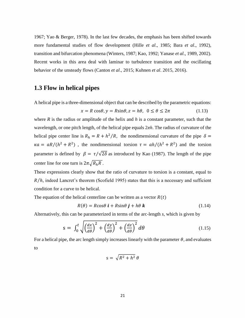
A helical pipe is a three-dimensional object that can be described by the parametric equations:

𝑥 = 𝑅 cos𝜃, 𝑦 = 𝑅sin𝜃, 𝑧 = ℎ𝜃, 0 ≤ 𝜃 ≤ 2𝜋 (1.13)

where R is the radius or amplitude of the helix and h is a constant parameter, such that the

wavelength, or one pitch length, of the helical pipe equals 2πh. The radius of curvature of the

helical pipe center line is 𝑅ℎ = 𝑅 + ℎ2 𝑅⁄ , the nondimensional curvature of the pipe 𝛿 =

𝜅𝑎 = 𝑎𝑅 (ℎ2 + 𝑅2)⁄ , the nondimensional torsion 𝜏 = 𝑎ℎ (ℎ2 + 𝑅2)⁄ and the torsion

parameter is defined by 𝛽 = 𝜏 √2𝛿⁄ as introduced by Kao (1987). The length of the pipe

center line for one turn is 2𝜋√𝑅ℎ𝑅 .

These expressions clearly show that the ratio of curvature to torsion is a constant, equal to

𝑅 ℎ⁄ , indeed Lancret’s theorem (Scofield 1995) states that this is a necessary and sufficient

condition for a curve to be helical.

The equation of the helical centerline can be written as a vector 𝑅(𝑡)

𝑅(𝜃) = 𝑅cos𝜃 𝒊 + 𝑅sin𝜃 𝒋 + ℎ𝜃 𝒌 (1.14)

Alternatively, this can be parameterized in terms of the arc-length s, which is given by

s = ∫ √(𝑑𝑥

𝑑)2+ (

𝑑𝑦

𝑑)2+ (

𝑑𝑧

𝑑)2𝑑𝜃

𝑡

0 (1.15)

For a helical pipe, the arc length simply increases linearly with the parameter 𝜃, and evaluates

to

s = √𝑅2 + ℎ2 𝜃

22

The Frenet triad of tangent T, normal N and binormal B unit vectors of a curve R(s) are

defined as:

𝑻 = 𝑑𝑅

𝑑𝑠,𝑵 =

1

𝜅 𝑑𝒕

𝑑𝑠, 𝑩 = 𝑻 × 𝑵

where 𝛿 = 𝜖 = 𝜅𝑎 is the curvature introduced so far. Figure 1 shows several different helical

pipe geometries for varying parameter values, the properties of which are given in Table 1.1.

This figure indicates that one limit of a helical geometry is a straight pipe, and the other limit

is a toroidal pipe.

Table 1.1: Curvature and torsion data for helical pipes shown in Figure 1.1

Figure 1.1: Helical pipe with circular cross section

Pipe 2a [mm] h [mm] R[mm] δ τ β n

a 50.5 0 252.5 0.1 0 0 0

b 50.5 22.41 250.5 0.1 0.009 0.02 3.2

c 50.5 65.46 18.3 0.1 0.36 0.8 3.2

d 50.5 45.47 8.47 0.1 0.54 1.2 3

23

1.3.1 Non-orthogonal coordinate system

In the theoretical perspectives of the helical pipe flows, Wang (1981) formulated the Navier-

Stokes equations in a non-orthogonal helical coordinate system. This is shown in Figure 1.2,

and the key points are as follows.

The first axis of the coordinate system is given by the vector equation of the centerline:

𝑅 = 𝑋(𝑠)𝒊 + 𝑌(𝑠)𝒋 + 𝑍(𝑠)𝒌 (1.16)

where s is the arc length along the axis, and i, j, k are the standard unit vectors in a Cartesian

frame. A coordinate system (r, θ, s) can then be defined, such that a Cartesian vector x is

given by:

𝑥 = 𝑅(𝑠)𝑇 + 𝑟cos𝜃 𝑵(𝑠) + 𝑟sin𝜃 𝑩(𝑠) (1.17)

The definition of the pipe boundary follows naturally by setting 𝑟 = 𝐷 2⁄ , an additional

parameter that is the internal radius of the pipe. That is:

𝑥 = 𝑅(𝑠)𝑇 + (𝐷 2)⁄ cos𝜃 𝑵(𝑠) + (𝐷 2)⁄ sin𝜃 𝑩(𝑠) (1.18)

Taking the dot product of the incremental change of eqn (1.17) with itself gives:

𝑑𝑥. 𝑑𝑥 = (𝑑𝑟)2 + 𝑟2(𝑑𝜃)2 + [(1 − 𝜅𝑟 cos𝜃)2 + 𝜏2𝑟2](𝑑𝑠)2 + 2𝜏𝑟2𝑑𝑠𝑑𝜃 (1.19)

non-orthogonality

It is the last term in Eq. (1.19) which highlights the non-orthogonal nature of this coordinate

system. The physical consequence of this non-orthogonality is that the axial velocity w is not

perpendicular to the (r, θ) plane. Wang’s analysis assumes that the pipe is long enough for

end effects to be ignored, that is, the velocities are independent of s, or fully developed. In

addition, both the curvature and torsion are assumed to be small, with the flow steady and

laminar, for the Reynolds number of order unity.

For small curvature and torsion the axial flow w is dominant, and is found to be Poiseuille

flow. This allows a series expansion of the form

𝑤 = 𝑼 ∑ 𝜖𝑖𝑤𝑖𝑛𝑖=0 (1.20)

for the axial velocity, where U is a velocity scale proportional to the axial pressure gradient,

and 𝜖 = 𝜅𝑎 ≪ 1, for pipe radius a. The secondary flow velocity is expanded in the following

way, using u as an example:

𝑢 = 𝑼 ∑ 𝜖𝑖𝑢𝑖𝑛𝑖=1 (1.21)

24

The secondary flow is therefore order-1, with stream function 𝜓 defining the velocities as

𝑢1 =1 𝜕𝜓

𝜕, 𝑢2 = −

𝜕𝜓

𝜕 (1.22)

Figure 1.2: Helical coordinate system used by Wang

where η is the normalised radial position, r/a. The stream function solution is:

𝜓

𝑅𝑒=

sin

288(𝜂7 − 6𝜂5 + 9𝜂3 − 4𝜂) −

1

4(𝜆

𝑅𝑒) (𝜂4 − 2𝜂2 + 1) (1.23)

Dean vortices Torsion rotation

The first term in Eq. (1.23) is the stream function for the Dean vortices; a pure curvature

effect. The second term is a pure rotation, indicated by the lack of 𝜃 dependence, which arises

due to the effect of torsion on the flow, where 𝜆 = 𝜏 𝜅⁄ and is a constant of order unity.

Wang found that for 𝜆 𝑅𝑒 ≥ 1 24⁄⁄ torsion dominates, causing a single recirculation cell in

the secondary flow. It is important to note that this torsion effect is of first-order, which is

the same order as curvature. This is because ψ is an O(𝜖) term, a first order term in this

expansion, and 𝜆𝜖 = 𝜏𝑎

1.3.2 Orthogonal coordinate system

Germano showed that it is possible to construct an orthogonal coordinate system by replacing

θ, from Wang’s system, with θ +𝜙(s)+𝜙0, in the plane normal to the axis (Germano 1982),

as shown in Figure 1.3. The Cartesian vector x therefore becomes:

25

𝑥 = 𝑅(𝑠)𝑇 + 𝑟cos(𝜃 + 𝜙(𝑠) + 𝜙0) 𝑵(𝒔) + 𝑟sin(𝜃 + 𝜙(𝑠) + 𝜙0) 𝑩(𝑠) (1.24)

where 𝜙(𝑠) = −∫ 𝜏(𝑠′)𝑑𝑠′𝑠

𝑠0

with 𝜙0 and 𝑠0 taking arbitrary values. Again performing the dot product of the incremental

change as before:

𝑑x. 𝑑x = (𝑑𝑟)2 + 𝑟2(𝑑𝜃)2 + [1 + 𝜅𝑟 sin (𝜃 + 𝜙]2(𝑑𝑠)2 (1.25)

which shows that the system is now orthogonal. The key result reported in this

Figure 1.3: Helical coordinate system used by Germano

paper is that the torsion has only a second order effect on the flow, contrary to the findings

of Wang (Wang 1981). Germano’s orthogonal formulation was subsequently used by many

researchers. It has also been used to analyses flow in pipes with non-uniform curvature and

torsion. Kao (1987) used it to obtain a series expansion for small Dean number flows, but

with the term 𝛽1 2⁄ = O(1),where 𝛽1 2⁄ = 𝜆 (2𝜖)1 2⁄⁄ . The series expansions are of the form:

𝑤 = 𝑤0 + ∑ 𝐷𝑛(1+𝑖) 2⁄ 𝑤𝑖∞𝑖=1 (1.26)

for the axial velocity w, and for the streamfunction 𝜓

𝜓 = 𝜓0 + ∑ 𝐷𝑛(1+𝑖) 2⁄ 𝜓𝑖∞𝑖=1 (1.27)

where the leading order solution is the Poiseuille flow, 𝑤0 = 1 − 𝑟2 and 𝜓 = 0. It should be

noted that the stream function 𝜓 is of a modified form, shown in Eq. (1.27), which is

introduced to replace the continuity equation (to make the system analogous with Dean’s

formulation, and identical if β = 0).

26

𝑢 = 1

𝑟

𝜕𝜓

𝜕𝛼− 𝛽1 2⁄ 𝐾1 2⁄ 1

𝑟∫ 𝑟𝑟

0

𝜕𝑤

𝜕𝛼𝑑𝑟, 𝑣 = −

𝜕𝜓

𝜕𝑟 (1.28)

It is clear that the second term in u, in Eq. (1.28), shows that the stream function is not a ‘true’

stream function. This shows that the secondary flow cannot be represented by the contours

of the stream function, but must be represented by velocity vector plots of (u, v). This is a

direct consequence of using Germano’s orthogonal coordinate system, whereas Wang’s non-

orthogonal system did allow a pure stream function representation of the secondary flow.

The results suggest that if 𝛽1 2⁄ = O(1), torsion term is in the order of 3/2 terms in the

expansion, otherwise, it is second order, as reported by Germano (1982).

Kao (1987) then presented numerical solutions, valid for moderate Dean numbers, which

show that if curvature is not small, even for values of 𝛽1 2⁄ as low as 0.1, significant distortion

of the secondary flow is found, to the extent that the second vortex is confined to a very small

region near the wall. This is qualitatively similar to the results reported by Wang (1981).

Germano returned to the problem of helical pipes (Germano 1989), but on this occasion, used

an expansion in the Dean number, rather than curvature as in the original paper (Germano

1981). The formulation is such that if there is no torsion, the original Dean equations are

recovered. Investigating further the influence of torsion, Germano also examined geometries

that possessed an elliptical cross-section, rather than a circle. The solutions obtained show

that for an elliptical boundary, the effect of torsion on the secondary flow appears in the first-

order terms of the expansion. In the special case of a circular boundary, the first-order terms

disappear, and the effect is reduced to second-order.

Clearly, the literature examined so far is regarding the question of the order of the effect of

torsion. The problem was finally resolved by Tuttle (Tuttle 1990). It is explained that Wang

and Murata (1981) both used non-orthogonal co-ordinate systems, requiring a covariant

tensor treatment to derive the Navier-Stokes equations. However, Wang focused on the

contravariant velocities (which permitted a stream function definition) whereas Murata

examined the covariant components. Since Germano’s co-ordinate system is orthogonal, the

co- and contravariant vectors are equivalent. Tuttle shows that simple transformations relate

the velocities defined in each co-ordinate system, so that Wang and Germano were both

actually considering the same velocity field, but from different perspectives.

27

Tuttle concludes that the appropriate co-ordinate system for understanding the effect of

torsion is Wang’s system, whilst acknowledging that it is more convenient to work with

Germano’s formulation, as the co- and contravariant vectors are identical and easier to

understand. Tuttle’s analysis therefore supports Wang’s original conclusion that the effect of

torsion is first order that is of the same order as curvature.

Liu & Masliyah (Liu 1993) analyzed the Navier-Stokes equations for the flow in a loosely

coiled helical pipe. Loose coiling can be achieved through a large helical radius or large pitch,

specifically they assume:

κa → 0, τa→ 0, Re→ +∞, κa ≠ 0

This reveals two dimensionless quantities that govern the flow. The first, the Dean number

has already been discussed, and the second is the Germano number, Gn. Physically, Gn

expresses the relative strengths of the effects of twisting, ρη𝑈2, and viscosity, 𝜇𝑈, that act on

the flow, thus measuring the torsion effect. It is defined as:

Gn = Reτa

By considering the effect of Gn in terms of the secondary flow structure, two further

dimensionless groups become significant. For large Dean numbers the dimensionless

parameter γ must be large for Gn to have a noticeable effect on the flow, where γ is defined

as:

𝛾 =𝐺𝑛

𝐷𝑛32

=𝜏𝑎

(𝜅𝑎𝐷𝑛)12

(1.29)

For small Dean numbers, Dn < 20, the equivalent group is 𝛾∗

𝛾∗ =𝐺𝑛

𝐷𝑛2=

𝜏𝑎

(𝜅𝑎)12 𝐷𝑛

=𝜅𝑎𝑅𝑒

(1.30)

Their results show that the secondary flow transition from two vortices to one vortex at 𝛾∗>

0.039, when Dn < 20, and at γ > 0.2 for Dn ≥ 20. Unique by amongst the studies discussed

so far, Liu & Masliyah also examined the axial wall shear rate distribution, for varying torsion

(keeping curvature ratio and Dean number fixed). It was shown that for small γ the shear rate

is largest near the outer wall, but as 𝛾 increases, the maximum value moves to the inner upper

28

wall. For large 𝛾 the distribution is approximately uniform, which would be valuable in a

biological context, suggesting one possible evolutionary advantage to non-planar geometries.

1.4 Flow pattern through curved and helical pipes

Although the systematic theoretical and experimental exploration of flow in curved conduits

is of a fairly recent origin, it has long been appreciated that the flow is considerably more

complex than that in straight conduits. The earliest observation of this was in fact for open

channel flow, where the effects of curvature are most evident and striking (Thomson 1876-

77]. In this century, Grindley and Gibson (1908) noticed the curvature effect on the flow

through helical pipes during experiments on the viscosity of air. It was noted by Williams et

al. (1902) that the location of the maximum axial velocity is shifted toward the outer wall of

a curved pipe. Later, an increase in resistance to flow for the curved tube compared to the

straight tube was observed by Eustice (1910) and this increase in resistance could be

correlated to the curvature ratio. However, in coiling the tubes, considerable deformation

occurred in the cross section of the tubes for some of the trials, causing an elliptical cross-

sectional shape.

Eustice (1911) also noted that the curvature, even slight, tended to modify the critical velocity

that is a common indicator of the transition from laminar to turbulent flow. By using ink

injections into water owing through coiled tubes, U-tubes and elbows, He observed the

pattern of the secondary flow. This secondary flow appears whenever a fluid flows in a

curved pipe or channel. Motivated by these findings, Dean (1927-28) undertook an analytic

study of steady, fully developed flows in curved pipes of circular cross section using regular

perturbation methods. Dean simplified the governing equations (later termed the “Dean

approximation”) by neglecting all effects arising due to pipe curvature except the centripetal

acceleration terms. This approximation reduced the number of non-dimensional parameters

from two (Reynolds number and the curvature) to a single non-dimensional parameter, the

Dean number, Dn = Re𝛿0.5 . The experimental work of Eustice and the mathematical

formulations of Dean set the foundations for, essentially, all subsequent work in this area.

Although Dean's approach was limited to the lower range of laminar flow in a torus of small

29

curvature, he clearly noticed these limitations and suggested approaches to extend the results

to turbulent ow. Even at this early stage, Dean and Eustice had recognized several of the

consequences of tube curvature on fluid flow that received more detailed attention in the

following decades. Among these were the facts that there is no clear critical Reynolds number

at which the demarcation between laminar and turbulent flow arises and that the onset of

turbulence occurs at a substantially higher Reynolds number than in a straight pipe. White

(1929) extended the work of Dean to coiled pipes and confirmed that the transition from

laminar to turbulent flow depends on the coil curvature. Masliyah (1980) studied the flow

field under the laminar condition in a helical semicircular duct by numerically solving the

Navier-Stokes equations. With the plane wall of the duct being the outer wall, the solution of

the momentum equations for Dn < 105 gave, for the secondary flow, twin counter-rotating

vortices. However, for Dn = 105, two solutions were obtained. One solution was similar to

that obtained for Dn < 105 and the other solution revealed four vortices for the secondary

flow. Flow visualization confirmed the possibility of the presence of both types of secondary

flow patterns. Nandakumar and Masliyah (1982) further studied this phenomena and reported

that using a bipolar-toroidal coordinate system worked better for predicting the four-vortex

solution. They showed that, for flow in helical tubes bifurcation exists irrespective of the

shape of the tube. However, it was much easier to obtain a dual solution when the outer

surface is nearly flat. Dennis and Ng (1982) performed numerical solutions of the Navier-

Stokes equations for steady laminar flow through a slightly curved tubes of constant circular

cross-section, using a finite difference method within the Dean number range of 96 < Dn <

5000. For Dn < 956 only one solution was found for a given Dean number. The secondary

flow consists of a symmetrical pair of counter-rotating vortices. While, for values of Dean

numbers above 956, two solutions were obtained one of them with two vortices and the

second has a four-vortex pattern. An analytical study on the flow Reynolds number flows of

a magnetic fluid through a helical pipe was conducted by Verma and Ram (1993). They found

that to the order considered, torsion does not affect the flow rate and also acknowledged that,

owing to the non-zero curvature, the flow rate cannot be expressed in terms of Dean number

alone. The unsteady flow in a pipe of circular cross-section which is coiled in a circle was

studied by Lyne (1970), the pressure gradient along the pipe was varying sinusoidally in time

30

with frequency. It was found that the secondary flow in the interior of the pipe was in the

opposite sense to that predicted for a steady pressure gradient, and this was verified

qualitatively by an experiment. A parallel effort by Zalosh and Nelson’s (1973) has appeared

to study unsteady pulsating flows in curved tubes for fully developed laminar flows with

pressure gradients that oscillated sinusoidally in time. Lyne (1970) has treated the case where

the frequency parameter is large, while Zalosh and Nelson study was dealing with small,

moderate and large values of the frequency parameter. Three different solutions have been

presented. The results revealed that the secondary flow is composed of a steady component

and a component oscillating at the second harmonic of the applied pressure gradient. The

secondary-flow reversal noted by Lyne (1970) has also been found. Whalley (1980) studied

experimentally air-water two-phase flow in a helically coiled tube. The flow pattern transition

between stratified and annular flow was examined, and a series of measurements were then

taken in the annular flow regime. Local values of the liquid thickness and liquid flow rate

around the tube periphery were obtained. The variations of these values around the periphery

was similar. The results showed that, for most of the cases studied the liquid flow rate was

greatest on the inside of the bend, but in some results a subsidiary peak at the outside position

was also obtained. There was little net entrained flow because of the centrifugal forces

tending to more drops very quickly.

An experimental investigation was carried out by Anwer et al. (1989) to study the effect of

bend curvature on a fully developed turbulent pipe flow. The pipe Reynolds number and the

pipe-to-bend radius ratio were 50 000 and 0.077, respectively. Results showed that a Dean-

type secondary motion was established in the bend and was confirmed by a numerical

modeling of the flow based on a two-equation closure. Evidence of a second cell was obtained

within the bend and again verified by numerical results and previous total pressure

measurements. They explained that the turbulent kinetic energy was greatly enhanced by

additional production due to extra strain rates created by bend curvature and that viscous

dissipation was the only way in which this extra energy can be destroyed, therefore, recovery

from bend curvature takes a long distance. Anwer and So (1993) conducted an experimental

study of a swirling turbulent flow through a curved pipe. The measurements were used to

analyze the competing effects of swirl and bend curvature on curved-pipe flows, particularly

31

their influence on the secondary flow pattern in the cross stream plane of the curved pipe.

They found that the superimposed solid-body rotation (swirl) completely dominated the

secondary flow, though they used a strong swirl and this may not be the case for weaker

swirls. They also found that wall static pressure was lower on the outer bend than in the inner

bend, which contradict with the normal secondary flow caused by curvature Boersma and

Nieuwstadti (1996) used large-eddy simulation (LES) to study the flow pattern of a fully-

developed turbulent flow in a curved pipe. The effect of curvature on the mean velocity

profile was presented and also various turbulent statistics. They found that the secondary

flow patterns consist of two strong counter rotating vortices near the inside of the bend which

are driven by the centrifugal force. The results showed that the turbulence intensities were

enhanced at the outside of the bend and suppressed at the inside, which was consistent with

observations in a curved channel flow. Furthermore, it was shown that the turbulent Reynolds

stresses were large in the core region of the pipe, in contrast to straight pipe flow where the

Reynolds stresses are small in this region. A reasonable agreement with the experimental

results from literature was found. Park et al. (1999) measured the axial and radial velocity

fields in the plane of symmetry of a 90o curved tube using laser photo chromic velocimetry

combined with a technique involving a simple interpolation and local modeling. This

technique was also used to estimate the wall shear stress, the vorticity, and the pressure field.

Experimental investigations on oil-air-water three-phase flow were carried out by Chen and

Guo (1999) in helically coiled tubes to provide a basis for the invention and development of

a new kind of separation technology for gasoil- water mixtures with low oil fraction. The

flow patterns of oil-water two-phase flow and oil-air-water three-phase flow were directly

observed in test sections made of plexiglas tubes. The flows observed in coiled tubes could

be classified into more than four flow patterns. The results were compared with some results

in horizontal flow. Correlations for the predictions of pressure drop were obtained. Huttl and

Friedrich (2000 and 2001) used direct numerical simulations to study fully-developed, steady

turbulent flow in straight, curved and helically coiled pipes. It was shown that pipe curvature

which induces secondary flow has a strong effect on the flow pattern. Turbulence was

significantly inhibited by streamline curvature and the flow almost relaminarized for large

32

values of the curvature. The results revealed that, the torsion effect was found to be weaker

than the curvature effect, but cannot be neglected.

1.5 Influence of pitch on the flow pattern An orthogonal coordinate system along a generic spatial curve has been introduced by

Germano (1982) to study the effect of torsion and curvature on the flow in a helical pipe. The

result showed that for curvatures and torsion are of the same order and for low Reynolds

numbers the curvature induces a first-order effect on the flow, while the effect of the torsion

on the flow is of the second order. This last result disagrees with those of Wang (1981), who,

adopting a non-orthogonal coordinate system, found a first-order effect of torsion on the flow.

The difference between the two studies was attributed to the difference in the coordinate

system used. Further studies by Germano (1989) confirmed that the torsion had no first order

effect on the flow in a helical pipe with circular cross-section. However, in the case of a

helical pipe of elliptical cross section there was a first order effect of the torsion on the

secondary flow. A study of the torsion effect on the fully developed laminar flow in a helical

pipe of constant circular cross section was conducted by Kao (1987). The results indicated

that, as far as the secondary flow patterns are concerned, the presence of torsion can produce

a large effect if the ratio of the curvature to the torsion is of order unity. In these cases the

secondary flow, though still consisting of a pair of vortices, can be very much distorted.

Under extreme conditions one vortex was so prevalent as to squeeze the second one into a

narrow region. However, generally the torsion effect was small and the secondary flow has

the usual pattern of a pair of counter-rotating vortices of nearly equal strength. He also

showed that, concerning the flow resistance in the pipe the effect of torsion is always small

in all the circumstances that have been considered.

Xie (1990) investigated the steady, fully developed laminar flow in a helical pipe by the

perturbation method using a helical coordinate system. Results showed that the torsion of the

pipe has only a second-order effect, which causes the secondary vortices to turn and deform.

33

In some cases of low Reynolds numbers, the dividing line between the two vortices could be

inclined so much that it is almost vertical. A study of the effect of pitch and torsion on the

secondary flow fields for fully developed laminar flow was performed by Liu and Masliyah

(1994) and showed that the critical value for the transition of two vortices to a single vortex

was based on the Dean number, the normalized curvature ratio, and the normalized torsion.

The pressure drop and friction factors were also studied for fully developed laminar flow.

The results for the pressure drop and the friction factor were further validated by experimental

results of Liu et al. (1993). Huttl and Friedrich (1999) used direct numerical simulations to

study the effects of curvature and torsion on turbulent flow in helical coils. It was shown that

the torsion increased the secondary flow effect and tended to change its pattern, while having

negligible effects on the axial velocity. On the other hand, curvature tended to decrease the

turbulent kinetic energy compared to a straight pipe flow.

1.6 Stability of the flow in a helical pipe

Fluid flow in helical pipes appears in many engineering processes particularly those

involving pipe systems for transport and treatment of gases and liquids. As an initiator, Dean

first studied the flow in a curved pipe in 1927 using a concentric toroidal coordinates system.

Since then a lot of researches have been made theoretically, numerically, and experimentally

and attracted great interest. For example, Nandakumar & Masliyah (1982) dealt with the flow

in a torus and documented the flow and dimensionless radius of curvature. One of the

interesting features of the flow through a toroidal pipe has been found unexpectedly by

Dennis & Ng (1982) and Yanase et al. (1989), which is the appearance of dual or more

solutions if the Dean number exceeds a certain critical value. The stability of flows in a torus

has been studied by Yanase et al. (1989).

Yanase et al. (1989) numerically performed the dual solution of the laminar flow through a

toroidal pipe with circular cross section. In the steady calculations, they obtained a four-

vortex structure of secondary flow tends to an almost two-vortex structure due to the

instability of toroidal pipe flow by use of the spectral method assuming that the flow field is

34

uniform in the axial direction of the toroidal pipe. They obtained the formula for the friction

factor of a toroidal pipe, which covers the wide region from low to high Dean numbers.

Laminar flow in helical pipes has been treated less extensively. Although a helical pipe

involves an additional parameter compared with the curved pipe, which naturally increases

its complexity. The main reason impeding the progress of the research in a helical pipe in

using a non-orthogonal coordinate system. Owing to the non-orthogonality of the coordinates,

problems may arise in the analysis, numerical calculation and the interpretation of the results

between two coordinates systems. To avoid the complexity associated with the non-

orthogonal helical coordinates system, Germano (1982, 1989) introduced a helical

coordinates system. The advantages of orthogonal helical coordinates system in not only the

simplification of the basic equations but also it makes the comparison with that of a curved

pipe much clear. Based on the helical coordinate system, Yamamoto et al. (1994) made some

numerical analysis on the helical pipe flow over the wide range of the Dean number.

The literature examined so far has only considered laminar flow, but there are some papers

that have investigated the transition to turbulence in helical pipe flow. It is known that the

flow in curved pipes is far more stable than that in a straight pipe (Taylor 1929) (White 1929).

Sreenivasan and Strykowski (1982) studied the stabilization effects in flow through helically

coiled pipes with negligible torsion and showed that, it is possible that the curvature in a pipe

flow somehow acts as a filter that removes the most critical disturbances, or at least

diminishes their amplitude, alter the frequency or both, in such a way that the remainder of

the disturbances does not become unstable until after a fairly high value of the Reynolds

number is attained.

Yamamoto et al. (1994) numerically investigated helical pipe flow by use of the spectral

method assuming that the field is uniform in the axial direction of the helical pipe. In their

comprehensive numerical study, vector plots of the secondary flow and axial flow

distributions were shown for large Dean numbers with fairly large curvature and torsion. In

the study, they found that two-vortex structure of secondary flow in a toroidal pipe tends to

almost single-vortex structure as torsion increases. They also found that if the pipe is toroidal,

35

the maximum axial velocity lies on the horizontal line, whereas the maximum velocity

position moves away from the horizontal line if torsion increases.

Yamamoto et al. (1995) experimentally investigated the laminar to turbulent transition of the

helical pipe flow. They found that the addition of torsion had a destabilizing effect on the

laminar flow. The critical Reynolds number of the laminar to turbulent transition decreased

with increasing torsion until it reached minimum. Then, it increased with further increasing

torsion. The minimum critical Reynolds number was far below that of a straight pipe. More

specifically, for three different dimensionless curvatures (0.01, 0.05, 0.1), increasing a

torsion parameter reduces the critical Reynolds number, with a minimum occurring for β in

the range 1.3−1.4. The lowest critical Reynolds number was found to be approximately 400

at β = 1.4 when δ = 0.1 (note, that here, the critical Reynolds number indicates the start of

transition, rather than flow is turbulent). They suggest that this behavior is directly linked

with the transition from two vortices to one vortex in the secondary flow.

Yamamoto et al. (1998) further numerically studied, by way of the 2D linear stability analysis

with the spectral method as the initial condition of the steady solution is also performed, and

obtained results that were in general agreement with the experiment data of Yamamoto et al.

(1995). However, the critical Reynolds number is found to be consistently lower in the

numerical study. It is thought that this is due to the time needed for the disturbances at the

inlet to grow large enough for the hot-wire to detect in the experimental configuration. By

use of periodic in- and outflow boundary conditions, Huttel et al. (1999) obtained secondary

and axial flow for a helical pipe at low torsion parameter by the finite volume method.

However, they did not discuss the destabilizing effect of torsion on the helical pipe flow.

In another paper by Yamamoto et al. (2002) experimental and numerical results are presented

that visualize the flow structures in helical pipes. Once again, increasing torsion causes a

transition from a two vortex structure to a single vortex. The smoke injection results confirm

their previous work on turbulent transition, as when the Reynolds number reached 900 the

smoke is mixed by turbulence, and no longer provides effective visualization of the flow.

Tracking particles through a numerical velocity field (obtained in Yamamoto et al. (2000))

gives good agreement with the experiments.

36

An experimental investigation regarding the laminar to turbulent flow transition in helically

coiled pipes with negligible torsion was performed by Cioncolini and Santini (2006). The

influence of curvature on the laminar to turbulent flow transition was analyzed from direct

inspection of the experimental friction factor profiles obtained for twelve coils. They found

that, coil curvature was effective in smoothing the emergence of turbulence and in increasing

the value of the Reynolds number required to attain fully turbulent flow, with respect to

straight pipes. The results showed that, with strongly curved coils, namely for ratios of a coil

diameter to a tube diameter ranging from 6.9 to 24, the process of turbulence emergence is

so gradual that only one irregular behavior were observed in the friction factor profile,

actually marking the end of the turbulence emergence process. With intermediate curvature

coils, namely for ratios of a coil diameter to a tube diameter ranging from 35.3 to 103.7, the

process of turbulence emergence is still very gradual but the friction factor profiles exhibit a

more complicated pattern a part of which was apparently not observed in the previous

research. A mild curvature, namely a ratio of coil 25 diameter to a tube diameter ranging

from 153 to 369, was found effective in smoothing the emergence of turbulence only in the

very beginning of the emergence process.

Recently, Hayamizu et al. (2008) reported more accurate experimental data as for the critical

Reynolds number of the laminar to turbulent transition in helical pipe flow and found good

agreement with 2D spectral results of Yamamoto et al. (1998) for limited dimensionless

curvature.

In summary, in the steady calculations, the secondary flow of helical pipes is either a pair of

counter-rotating vortices with asymmetry, or a single vortex, and the axial velocity is non-

axisymmetric. Since curvature has a stabilizing influence and torsion has a destabilize effect

on the laminar flow in a helical pipe, the critical transition Reynolds number is reduced

significantly.

1.7 Pressure drop and friction factor

The main disadvantage of using curved and helical pipes is the increase of the flow resistance

due to the curvature, which mean greater pressure drop for the same volume flux as compared

37

to straight pipes. Pressure drop usually calculated using the friction factor, f, for which many

correlation formulae have been developed.

Ito (1959) presented data for isothermal flow of water through smooth curved pipes with

curvature ratios from 1/16.4 to 1/648 to determine the friction factors for turbulent flow. The

flow Reynolds number ranged for 103 < Re < 105 covering both laminar and turbulent

regions. He used both the 1/7th power velocity distribution law and the logarithmic velocity

distribution law to deduce resistance formulae for turbulent flow. It was found that for values

of Re 𝛿2 < 0.34 the friction factor in curved and helical pipes, 𝑓𝑐, was equivalent to that of a

straight pipe, 𝑓𝑠. For 0.34 < Re 𝛿2< 300 the resistance law is as follows:

𝑓𝑐𝛿−0.5 = 0.00725 + 0.076[𝑅𝑒 𝛿2]−0.25 (1.31)

However, for large values of Re 𝛿2, the following empirical equation was presented:

𝑓𝑐𝛿−0.5 =

0.079

[𝑅𝑒 𝛿2]0.2 (1.32)

Barua (1963) analyzed the motion of flow in a stationary curved pipe for large Dean numbers.

The analyses assumed a non-turbulent core where fluid moved towards the outer periphery,

and within a thin boundary layer fluid moved back to the inner periphery of the tube. A

relationship between the friction factor of a curved tube and a straight tube was made based

on Dn. This was compared to the experimental observations of other authors and was found

to be in fairly good agreement. The agreement was better for higher values of Dn than for

low values.

Akagawa et al. (1971) measured the frictional pressure drop of an air-water two-phase flow

in helically coiled tubes with different curvatures and found that the frictional pressure drop

in these coils was 1.1 to 1.5 times as much as that in a straight pipe. Kasturi and Stepanek

(1972) carried out measurements of pressure drop and void fraction for the gas-liquid two-

phase flow in a helical coil. The pressure drop results were fitted with the Lockhart-Martinelli

correlation but there was a systematic displacement of the curves for the various systems with

the Lockhart-Martinelli plot. Tarbell and Samuels (1973) solved the equations of motion and

heat transfer in curved tubes numerically by the alternating direction-implicit technique. A

friction factor correlation which properly accounts for the effect of curvature is developed to

be valid in the range 20 < Dn < 500. The resulting correlation is given below.

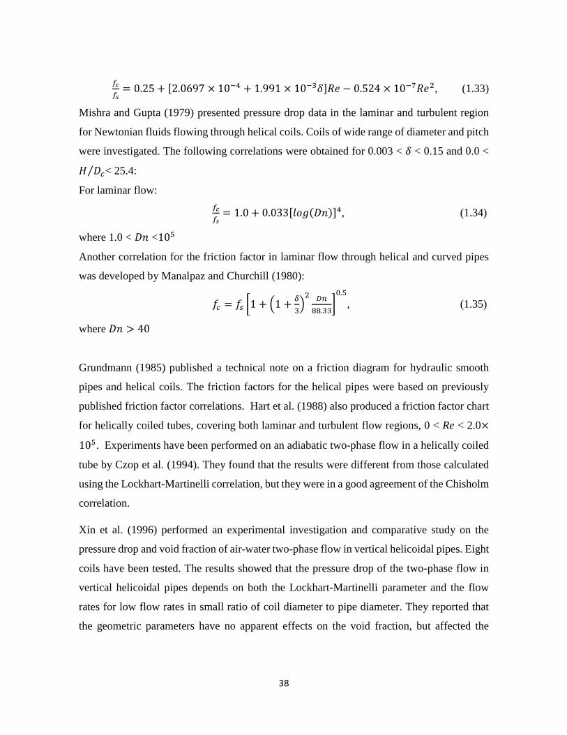
38

𝑓𝑐

𝑓𝑠= 0.25 + [2.0697 × 10−4 + 1.991 × 10−3𝛿]𝑅𝑒 − 0.524 × 10−7𝑅𝑒2, (1.33)

Mishra and Gupta (1979) presented pressure drop data in the laminar and turbulent region

for Newtonian fluids flowing through helical coils. Coils of wide range of diameter and pitch

were investigated. The following correlations were obtained for 0.003 < 𝛿 < 0.15 and 0.0 <

𝐻 𝐷𝑐⁄ < 25.4:

For laminar flow:

𝑓𝑐

𝑓𝑠= 1.0 + 0.033[𝑙𝑜𝑔(𝐷𝑛)]4, (1.34)

where 1.0 < 𝐷𝑛 <105

Another correlation for the friction factor in laminar flow through helical and curved pipes

was developed by Manalpaz and Churchill (1980):

𝑓𝑐 = 𝑓𝑠 [1 + (1 +𝛿

3)2 𝐷𝑛

88.33]0.5

, (1.35)

where 𝐷𝑛 > 40

Grundmann (1985) published a technical note on a friction diagram for hydraulic smooth

pipes and helical coils. The friction factors for the helical pipes were based on previously

published friction factor correlations. Hart et al. (1988) also produced a friction factor chart

for helically coiled tubes, covering both laminar and turbulent flow regions, 0 < Re < 2.0×

105. Experiments have been performed on an adiabatic two-phase flow in a helically coiled

tube by Czop et al. (1994). They found that the results were different from those calculated

using the Lockhart-Martinelli correlation, but they were in a good agreement of the Chisholm

correlation.

Xin et al. (1996) performed an experimental investigation and comparative study on the

pressure drop and void fraction of air-water two-phase flow in vertical helicoidal pipes. Eight

coils have been tested. The results showed that the pressure drop of the two-phase flow in

vertical helicoidal pipes depends on both the Lockhart-Martinelli parameter and the flow

rates for low flow rates in small ratio of coil diameter to pipe diameter. They reported that

the geometric parameters have no apparent effects on the void fraction, but affected the

39

frictional pressure drop. A correlation for frictional pressure drop multiplier for small coils

was provided based on the experimental data.

Sarin (1997) studied the fully developed steady laminar flow of an idealized elastico-viscous

liquid through a curved tube with elliptic cross section. It was shown that if the curvature of

the pipe was increasede, there will be delay in setting up a secondary motion. The shear stress

was found to be larger at the major axis and the outer bend than at the minor axis and the

inner bend. The curvature seemed to increase the wall shear stress on the outside wall and to

decrease it on the inside wall. The influence of helix axial inclination angle to the horizontal

plane on the fractional pressure drop of single phase water and steam-water two-phase flows

were studied in a pressure range of 3.0-3.5 MPa by Guo et al. (2001). Two helically coiled

tubes were employed as test sections and their four different helix axial inclinations were

examined. It is found that helix axial angles have little influence on the single-phase frictional

pressure drop, while variation of the steam-water two-phase flow frictional pressure drop was

enlarged to 70%. In a further study the same authors examined the two-phase flow of steam-

water to characterize pressure drop oscillations in a closed loop steam generator system

(2001).

Ali (2001) developed a correlation between pressure drop and flow rate for helical coils by

using the Euler number, the Reynolds number and a new geometrical number which is a

function of the equivalent diameter of the coil (taking pitch into account), the inside diameter

of the tube, and length of the coiled tube. He suggested that there are four regions of flow, a

laminar, a turbulent and two ranges of transitional flow.

1.8 Heat transfer of flow through curved and helical pipes Seban and McLaughlin (1963) performed an investigation of heat transfer in coiled tubes for

both laminar and turbulent flows. They used two Type 321 stainless steel tubes of 7.4 mm

inside diameter and 0.3 mm wall thickness. One tube was formed into a coil with 6.5 turns

and 125.2 mm diameter, the other was formed into 1.5 turns with 764.5 mm diameter.

Freezene oil was used to study heat transfer in laminar flow, whereas water was used to study

the turbulent range. Heat input and flow rate were varied in each case. For the oil, the Prandtl

40

number ranged tram 100 to 657, and the Reynolds number ranged from 12 to 5600. For water,

the Prandtl range was 2.9 to 5.7 and the Reynolds range was 6000 to 65600.

For laminar flow the results showed that the outer periphery had higher Nusselt numbers than

the inner (ratio of roughly 4:1 for the curvature ratio of 1/17), with both being substantially

higher than theoretical Nusselt numbers for a straight pipe under the same conditions. The

results also indicated the effect on the Nusselt numbers due to a thermal entry length. One of

the interesting results of this study was that although the local heat transfer coefficients

dropped from inlet towards outlet, there was a tendency for them to rise at the last

measurement position (near the outlet). This was attributed to a buoyancy effect because the

increase appeared to be relatively greater at higher heat flux input. They proposed the

following equation for case of laminar flow:

ℎ𝑑𝑝

𝑘(𝑃𝑟)−1 3⁄ = 𝐶 [

𝑓

2𝑅𝑒2]

1 3⁄

, (1.36)

where C is a constant suggested to be 0.13 for the small coil, and 0.74 for the larger coil.

The same experimental setup and methods were used to determine the friction factor and the

Nusselt number relationships for turbulent flow of water in the same coils as mentioned above.

The ratios of the inside to outside periphery heat transfer coefficients were of the order of 2

and 4 for the coils with curvature ratios of 1/104 and 1/17, respectively. Seban and

McLaughlin (1963) compared their average coefficients to the following relationship and

found that there was no deviation greater than 10% and 15% for the coils with curvature

ratios of 1/104 and 1/17:

ℎ𝑑𝑝

𝑘(𝑃𝑟)−0.4 =

𝑓

2𝑅𝑒 (1.37)

Data on pressure drop and heat transfer to aqueous solutions of glycerol flowing in different

types of coiled pipes were presented for laminar flow by Kubair and Kuloor (1966). The

Reynolds numbers was in the range of 80 to 6000 with curvature ratios in the range of 1/10.3

to 1/27 with 7 to 12 turns. A steam bath was used to provide constant temperature wall

41

conditions on the outside of the coil. The authors also noted that the results for the interaction

between heat transfer rates and the Graetz number of Berg and Bonilla (1950) were opposite

to those of Seban and McLaughlin (1963). The authors (1966) speculated that this difference

might have been due to the fact that the two studies used different boundary conditions, one

being constant wall temperature (1950) and the other at constant heat flux (1963). One of the

coils used by Kubair and Kuloor had the same curvature ratio as one of the coils used by

Seban and McLaughlin. The results of Kubair and Kuloor coincided with those of Seban and

McLaughlin at low Graetz numbers, but deviated at higher Graetz numbers. An empirical

correlation was developed based for curvature, 𝛿, and the Graetz number (Gz):

𝑁𝑢 = [1.98 + 1.8 𝛿]𝐺𝑧0.7 (1.38)

in the range of 10 < Gz < 1000, 80 < Re < 6000 and 20 < Pr < 100.

The fully developed laminar convictive heat transfer and fluid flow in a curved pipe with a

uniform heat flux for large Dean numbers was investigated both theoretically and

experimentally by Mori and Nakayama (1965).

They assumed that the flow was divided into two sections, a small boundary layer near the

pipe wall, and a large core region making up the remaining flow. In the core region, the

secondary flow was assumed to be completely horizontal, transporting the fluid to the outside

of the pipe. The fluid returned to the inner wall through the boundary layer. This pattern

differed for that of small Dean numbers. By their theoretical analysis, they deduced that the

additional flow resistance of a curved pipe is caused by stress due to the secondary flow.

They also developed a ratio between the thickness of the temperature and velocity boundary

layers, expressed in terms of the Prandtl number. The Nusselt number ratio between straight

and curved pipes was shown to be a function of the Dean number and the ratio between the

thickness of the thermal and hydrodynamic boundary layers. Experiments performed with a

curvature of 1/40 were used to validate the theory. Profiles of both temperature and velocity

supported the theoretical analysis. Nusselt numbers calculated from experimental data were

shown to agree with those obtained theoretically. In their second report, Mori and Nakayama

(1965) studied the effect of curvature on flow field and heat transfer in fully developed

turbulent flow both theoretically and experimentally. Heat transfer was studied for the

constant heat flux system and the variations of physical properties with temperature were not

42

taken into account in the development. The analysis was performed assuming a thin boundary

layer along the pipe wall, similar to that in their previous report (1965).

Nusselt numbers averaged around the periphery were calculated. It was shown that the

difference between the Nusselt numbers for a straight and a curved pipe decreased slightly

as the Prandtl number became large, which is opposite to the results found for laminar flow

[1965, 1967]. Experiments were performed with air flowing through curved pipes with

curvature of 1/18.7 and 1/40. They extended their work (1967) to the theoretical analysis of

uniform wall temperature rather than uniform heat flux. The results show that the formula

for the Nusselt number of the uniform wall temperature is the same as that for uniform heat

flux. The Nusselt number relationships developed in the previous work (1965) for laminar

flow were presented in a more practical form. The change of physical properties with

temperature was studied for air, water, and oil. With the exception of laminar flow of water,

the mean temperature of the physical properties between the inlet and outlet could be used.

The correlations proposed for Nusselt number calculations were as follows:

I-Laminar flow:

𝑁𝑢 =0.864

𝐷𝑛0.5(1 + 2.35𝐷𝑛−0.5) (1.39)

where,

ζ =

{

2

11[1 + √(1 +

77

4

1

𝑃𝑟2)] for 𝑃𝑟 ≥ 1,

1

5[2 + √(

10

𝑃𝑟2)] for 𝑃𝑟 ≤ 1.

(1.40)

II-Turbulent flow:

For gases

𝑁𝑢 =𝑃𝑟

26.2(𝑃𝑟2 3⁄ −0.074)𝑅𝑒0.8𝛿0.1 [1 +

0.098

(𝑅𝑒𝛿2)0.2], (1.41)

where 𝑃𝑟 ≈ 1 and 𝑅𝑒𝛿2 > 0.1, while for liquids

𝑁𝑢 =𝑃𝑟𝑅𝑒

56𝛿

112

41.0[1 +

0.061

(𝑅𝑒𝛿2.5)1 6⁄ ], (1.42)

where, 𝑃𝑟 > 1 and 𝑅𝑒𝛿2.5 > 0.4.

43

Akiyama and Cheng (1971) studied the hydrodynamically and thermally fully developed

laminar forced convection in curved pipes subjected to the thermal boundary conditions of

axially uniform wall heat flux and peripherally uniform wall temperature at any axial position.

The Prandtl number effect on the heat transfer result was clarified, and it was shown that all

the heat transfer results for 𝑃𝑟 ≥ 1.0 can be correlated by a single curve using a new

parameter with reasonable accuracy. The results showed that as the Dean number increased,

the center of the secondary circulation moved towards the outer wall. However, in the

horizontal direction, it first begins to move towards the outer wall, but with further increase

of the Dean number, the center begins to move back towards the inner wall. From the

streamlines produced at the Dean number of 196, They suggested that the boundary layer

approximation that has been used by other researchers [Barua (1963), Mori and Nakayama,

1965] could not be applied. Akiyama and Cheng (1972) extended their work to include the

thermal boundary condition of uniform wall temperature. It has been shown that the heat

transfer results for fully developed laminar flow in curved pipes with the two basic thermal

boundary conditions of uniform wall temperature and uniform wall heat flux are quite similar.

For given Prandtl and Dean numbers, the Nusselt number for the uniform wall temperature

case became higher than that for the uniform wall heat flux case after reaching a certain Dean

number. This situation is opposite to that of a pure forced convection in a straight pipe.

Kalb and Seader (1972) studied theoretically the heat transfer to steady viscous flow in

curved pipe of circular cross section for fully developed velocity and temperature fields under

the thermal boundary condition of axially uniform wall heat flux with peripherally uniform

wall temperature. They found that the curvature parameter had negligible effect on the

average Nusselt number for any Prandtl number. However, the curvature ratio did have an

effect on the peripheral variation of the Nusselt number, though this effect was still not large.

For Pr > 0.7, it was shown that the local Nusselt number in the area of the inner wall was

always less than that of a straight tube, and increasing as the Dean number increased till it

reached a limiting value. The local Nusselt numbers on the outer wall continued to increase

with increasing Dean number. They also noted that the fractional increase in the heat transfer

coefficient is significantly greater than the fractional increase in friction losses, except for

44

liquid metals. The following Nusselt number relationship was developed for low Prandtl

numbers (0.005 to 0.05) with Dean numbers in the range of 20 to 1200:

𝑁𝑢 = (3.31𝐷𝑛0.115)𝑃𝑟0.0108 (1.43)

For Prandtl numbers in the range of 0.7 to 5 and Dean numbers of 80 to 1200, the following

average Nusselt number relationship was developed:

𝑁𝑢 = (0.913𝐷𝑛0.476)𝑃𝑟0.20 (1.44)

Kalb and Seader (1974) advanced this work by applying the method to the case of a uniform

wall-temperature. Their results showed that there exists a slight effect of curvature on the

peripheral variation of the Nusselt number. However, it did not affect the average Nusselt

number. As Akiyama and Cheng (1971) did, Kalb and Seader (1974) found that the thermal

boundary condition had a significant effect on the temperature field.

Austin and Seader (1973) numerically solved the equations of fluid motion for the case of

steady, fully-developed, isothermal, incompressible, viscous Newtonian flow in toroidal-type

coiled-tube geometry. However, the effect of coil pitch was not taken into consideration.

They speculated that the pitch effect might become important as the radius of curvature

approaches the radius of the tube. For low Dean numbers, the authors showed that the axial

velocity profile was essentially parabolic as in the straight tube case. As the Dean number is

increased, the maximum velocity began to be skewed toward the outer periphery. It was

shown that for Dn > 10.0, the maximum axial velocity on the horizontal axis tends to move

towards the outer periphery. Also they indicated that the pressure distribution is dependent

mainly on the Dean number and that the pressure increases smoothly from the inner to the

outer periphery. The axial pressure gradient was correlated to the friction factor, which

showed a slight dependence on the curvature ratio. The numerical results of the secondary

flow the center of the secondary flow vortex was close to the center of the tube horizontally

and situated slightly closer to the middle than the upper tube wall in the vertical direction.

The streamlines around the vortex were rather symmetrical. However, when the Dean

number was increased, the center of the vortex was seen to move upwards and inwards and

the streamlines lost their symmetrical form. Changing the curvature ratio had a slight effect

on the secondary flow streamlines for the same Dean number, indicating that the effect of

45

curvature ratio was almost completely accounted for in the Dean number. The numerical

results of Austin and Seader (1973) differed significantly from the model of Mori and

Nakayama (1965).

Patankar et al. (1974) investigated the three dimensional parabolic flows in a helical pipe

while they predict the velocity and temperature fields in helically coiled pipes. Predictions

were presented of flow and heat transfer in the developing and fully developed regions.

Comparisons of the developing and fully developed velocity profiles with experimental data

of Mori and Nakayama (1965) exhibited good agreement. The development of the wall

temperature for the case of axially uniform heat flux with an isothermal periphery has been

compared with experimental data and the agreement was also good. Predictions of fully

developed temperature profiles and heat transfer coefficients also exhibited close agreement

with experimental data of Mori and Nakayama (1965). Effects of the Dean number on the

friction factor and heat transfer were presented.

Yao and Berger (1978) conducted an analytical study of the fully developed laminar flow in

a heated curved pipe under the influence of both centrifugal and buoyancy forces. The pipe

was assumed to be heated so as to maintain a constant axial temperature gradient. Both

horizontal and vertical pipes were considered. Solutions for these two cases were obtained

by regular perturbations in the Dean number and the product of the Reynolds and the

Rayleigh numbers; the solutions were therefore limited to small values of these parameters.

Predictions of the axial and secondary flow velocities, streamlines, shear stress, temperature

distribution and heat transfer were given for a representative case.

The effect of buoyancy on the flow field and heat transfer was studied numerically by Lee et

al. (1985) for the case of fully developed laminar flow and axially constant heat flux with a

peripherally constant wall temperature. They found that the buoyancy acts to increase the

average Nusselt number, change the local Nusselt number distribution around the periphery

and rotate the orientation of the secondary flow velocity. Heat transfer coefficients of helical

coils in agitated vessels have been investigated by Havas et al. (1987). A modified Reynolds

number has been introduced into the heat transfer equation and a correlation was developed

for the Nusselt number on the outer wall based on the modified Reynolds number, the Prandtl

46

number, and the ratio of the diameter of the tube to the diameter of the vessel. In developing

this correlation, the calculations of the heat transfer coefficient on the outside of the pipe was

done by taking the total heat flux, temperature difference, and the internal heat transfer

coefficient.

Austen and Soliman (1988) studied the influence of pitch on the pressure drop and heat

transfer characteristics of helical coils for the condition of uniform input heat flux. The results

included the isothermal and adiabatic friction factors, wall temperature, and local and fully

developed Nusselt numbers. Significant pitch effects were observed in the friction factor and

Nusselt number results at low Reynolds numbers. These effects were attributed to free

convection, and they diminished as the Reynolds number increased.

Yang et al. (1995) presented a numerical model to study the fully developed laminar

convective heat transfer in a helicoidal pipe having a finite pitch. The effects of the Dean

number, torsion, and the Prandtl number on the laminar convective heat transfer were

discussed. The helicoidal pipe was assumed to have uniform wall heat flux with a uniform

peripheral wall temperature. The studied laminar flow of the incompressible Newtonian fluid

was subjected to be hydrodynamically and thermally fully developed. The results revealed

that the temperature gradient increased on one side of the pipe wall and decreased on the

other side with increasing torsion. In the case of a fluid with a large Prandtl number, the

Nusselt number significantly decreased as torsion increased, on the other hand, for a small

Prandtl number, the Nusselt number decreased slightly as the torsion increased.

Yang and Ebadian (1996) extended this research to turbulent flow using 𝑘 − 휀 model. As in

the laminar case, the torsion rotated and distorted the temperature profiles. The effects of

torsion could be enhanced by increasing the axial flow velocity.

Xin and Ebadian (1997) carried out experiments to investigate the effects of the Prandtl

number and geometric parameters on the local and averaged convective heat transfer

characteristics in helical pipes, with three different fluids air, water, and ethylene glycol on

five uniformly heated helical pipes. The ratios of the pipe diameter and pitch to coil diameter

ranged from 0.0267 to 0.0884 and 0.20 to 2.56, respectively. The peripheral and average,

fully developed Nusselt numbers were evaluated in the experiments. Experimental findings

indicated that after two turns the temperature distributions all dimensionless peripheral wall

47

temperatures are nearly identical, implying that both the flow and temperature distribution

within the helical pipes are fully developed. These results revealed that the peripheral Nusselt

number varies significantly for higher Prandtl numbers and Dean numbers in the laminar

flow region. A new set of empirical expressions established for the averaged fully developed

Nusselt number. No obvious effects of the coil pitch or torsion were observed in the scope of

the investigation.

Numerical studies were made of the flow and heat transfer characteristics of a fully-

developed pulsating flow in a strongly curved pipe by Chung and Hyun (1994). By using a

toroidal coordinate system, the complete, time-dependent incompressible Navier Stokes

equations were formulated. The peripherally uniform temperature condition was imposed on

the pipe wall. Particular attention is given to heat transfer properties over substantially

extended parameter ranges of the Reynolds number and the Womersley number (ratio of

transient inertial to viscous forces), which is a function of the pipe radius, the kinematic

viscosity, and the frequency of the pulsation. The computed results on the flow field were in

close agreement with the experimental data in the covering parameter ranges. The numerical

results showed that when Womersley number was small, the time and space averaged Nusselt

numbers, were lower for a pulsating flow than for a corresponding non-pulsating flow. At

moderate and high Womersley numbers, however, the difference in between a pulsating and

a non-pulsating flow was insignificant.

A further work on pulsating flow was performed by Guo et al (1998) for fully developed

turbulent flow in a uniformly heated helical coiled tube. In their work they studied both

pulsating flow and steady state flow. A series of correlations were proposed for the average

and local heat transfer coefficients both under steady and oscillatory flow conditions. They

noted that as the Reynolds number increased to very large values (Re > 140000), the heat

transfer coefficient for coils began to match the heat transfer coefficient for a straight pipe.

Correlation of the Nusselt number as a function of the Womersley number were also given.

Goering et al. (1997) used a two-dimensional numerical representation of the fully-elliptic

Navier-Stokes and energy equations to study the fully developed laminar flow through a

heated horizontal curved tube. The combined effects of curvature and buoyancy were

presented. Two thermal boundary conditions were used, both were with constant heat fluxes,

48

but one was with a constant peripheral heat flux while the other had a constant peripheral

wall temperature. Regime maps were presented for both boundary conditions which split the

heat transfer into three regimes; curvature dominant, buoyancy dominant, and an area where

both factors were important.

Bai et al. (1999) performed an experimental study on the turbulent heat transfer from

horizontal helically coiled pipe over a wide range of experimental parameters. They found

that as the Reynolds number increased, the effect of secondary flow on heat transfer

decreased, and the heat transfer approaches that of a straight pipe. This is due to the fact that

as the Reynolds number increases the boundary layer becomes smaller. They also found that

the local heat transfer coefficients on the outside wall was three or four times a than that on

the inside wall. A correlation was proposed to describe the local distribution of the of the

Nusselt number in the periphery.

Comparisons of the heat transfer coefficients between a straight pipe and helically coiled pipe

immersed in a water bath were performed by Prabhanjan et al. (2002). The purpose of this

study was to determine the relative advantage of using a helically coiled heat exchanger

versus a straight tube heat exchanger for heating liquids. Results showed that the heat transfer

coefficient was affected by the geometry of the heat exchanger and the temperature of the

water bath surrounding the heat exchanger. All tests were performed in the transitional and

turbulent regimes.

Inagaki et al. (1998) studied the thermal hydraulic characteristics of the gas to gas heat

exchanger with helically coiled tube bundles for Reynolds numbers in the range of 6000 to

22000. They developed a correlation for the Nusselt number on the outside wall as a function

of both the Reynolds and the Prandtl numbers.

𝑁𝑢 = (0.78𝑅𝑒0.51)𝑃𝑟0.30 (1.45)

A numerical study of the developing convective heat transfer in a coiled heat exchanger with

the effect of buoyancy was performed by Sillekens et al. (1998). Results showed that heat

transfer was highly influenced by the secondary flow and buoyancy forces. For low Grashof

numbers a splitting phenomenon of the temperature field was observed due to large

secondary velocities, resulting in two separated areas of fluid. However, for higher values of

49

the Grashof number, the fluid became almost linearly stratified which resulted in small

secondary velocities.

Zheng et al. (2000) studied the interaction phenomena between laminar forced convection

and thermal radiation in a participating medium inside a helical pipe numerically. The results

showed that under the conditions examined in this study, although the thermal radiation had

no significant influence on flow and temperature fields, it substantially enhanced the total

heat transfer in the helical pipe especially in a fully developed region.

Prabhanjan et al. (2004) conducted heat transfer studies of a helical coil immersed in a water

bath. A method to predict outlet temperatures from the helical coil was proposed which took

into consideration the flow rates and geometry of the coil. The heat transfer on the outside of

the coils was caused by natural convection. In this type of system, neither constant wall

temperature, nor constant wall heat flux could be assumed.

Simultaneous development of laminar Newtonian flow and heat transfer in helical pipes was

numerically studied by Liu and Masliyah (1994). The governing equations were fully

parabolized in the axial direction and were written in an orthogonal helical coordinate system.

The Nusselt number in the developing region was found to be oscillatory. The asymptotic

Nusselt number and the thermal entrance length are correlated with the Prandtl number and

the f Dean number. They showed that when torsion was dominant, the asymptotic Nusselt

number decreased while the thermal development length increased.

Developing laminar forced flow and heat transfer in the entrance region of helical pipes have

been investigated using a fully elliptic numerical method by Lin and Ebadian (1997b). The

results presented in this work covered a Reynolds number range of 250 to 2000, a pitch range

of 0.0 to 0.6, and a curvature range of 0.025 to 0.20. It has been found that both the friction

factor and the Nusselt number were oscillatory in the entrance region of helical pipes. These

oscillations were higher for lower curvature. The pitch and the Reynolds number exerted

different effects on the developments of the friction factor and the Nusselt number than the

curvature ratio. The same effects were numerically studied by Lin and Ebadian (1997b) for

the case of developing turbulent flow and observed the same oscillatory behavior of both the

Nusselt number and friction factor. However, they found that as the pitch, curvature or the

Reynolds was increased, these oscillations became stronger. Lin and Ebadian (1999)

50

numerically studied the effect of inlet turbulence intensity on the development of the

turbulent flow and heat transfer in helically coiled pipes. Their findings were that increased

inlet turbulence intensity tended to reduce the velocity gradient at the walls of the pipe

although it had negligible effect on the maximum axial velocity. Increasing the intensity level

also increased the intensity of the secondary flow but did not change its pattern. The thermal

boundary layer developed quicker with increased inlet turbulence intensity.

A fully elliptic numerical study was performed to investigate the buoyancy affected, three-

dimensional turbulent flow and heat transfer in the entrance region of a curved pipe by Li et

al. (1998). It was found that, at higher Grashof numbers, the developing secondary flow field

showed the existence of three vortices. The peripherally averaged Nusselt number and the

friction factor exhibited oscillatory behavior along in streamwise direction. The

augmentation of the average Nusselt number and the friction factor resulting from buoyancy

was prominent at the entrance region of the pipe, but gradually became weaker further

downstream.

Rindt et al. (1999) conducted a numerical study on the development of mixed convective

flow in a helically coiled heat exchanger with an axially varying wall temperature for

Reynolds number of 500, the Prandtl number of 5 and curvature of 1/14 and compared to the

constant wall temperature boundary condition. The influence of buoyancy forces on heat

transfer and secondary flow was presented. It was found that, for all Grashof numbers studied

it appeared that both heat transfer, quantified by the Nusselt number, and secondary flow,

quantified by the relative kinetic energy, and exhibited a wavy behavior in axial direction.

For higher Grashof numbers, however, this phenomenon diminished for the case with an

axially varying wall temperature due to stabilizing effects of stratification.

51

Chapter 2

2.1 Mathematical formulation and governing equations

The governing equations described below are the Navier-Stokes equations and heat

conduction equations. OpenFOAM reduces those PDE's into a set of linear algebraic

equations and solves them. In order to validate a CFD code, computational results must be

compared with some prepossessed knowledge (i.e., previous experimental data or numerical

result by spectral study). In the case that steady and transient solutions of helical circular

pipes can be derived, a foundation for validation is provided.

Any point of a helical pipe with circular cross section can be described by the coordinate

system (x, y, z), as shown in Fig. 2. The cross section of the helical pipe is a circle with the

internal diameter 𝑑𝑝(= 2a), and 𝐻 is one pitch length of the helical pipe. The unit tangential

vector, 𝒕, the unit normal vector, 𝒏, and the unit binormal vector, 𝒃, of the center line of the

pipe are defined, where 𝒃 = 𝒕 × 𝒏 (see Fig. 1(b)). The x-axis is to the direction of −𝒏, the y-

axis to the direction of −𝒃 and the z-axis is a taken along the center line of the pipe. The x,

y and z coordinates constitute the orthogonal coordinate system. The flow is driven by

constant pressure gradient along the center line of the pipe and the main flow direction is to

the positive z. A thick broken line denotes the center line of the helical pipe and R is the

distance of the center line from the axis of the whole system.

Then the continuity equation, the Navier-Stokes equations and heat conduction equation can

be written as:

𝛻 ∙ 𝑼 = 0, (2.1)

𝜕𝑼

𝜕𝑡+ (𝑼 ∙ 𝛻)𝑼 = −

1

𝜌𝛻𝑝 + 𝜈𝛻2𝑼, (2.2)

𝜕𝑻

𝜕𝑡+ (𝑼 ∙ 𝛻)𝑻 = 𝛼 𝛻2𝑻. (2.3)

52

Fig. 2.1. (a) Helical pipe with circular cross section, (b) coordinate system.

t n

b

a

R

Center line

x

y

z

Axis of the whole system

𝑅

𝐻

2𝑎

Inlet

Outlet

Axis of the whole system

𝑇𝑤 (Heated

wall)

𝑇𝑤 > 𝑇𝑖𝑛𝑡

53

The aforementioned numerical solutions can be found by reducing the governing equations

under these assumptions:

1. The flow is incompressible Newtonian fluid.

2. The pipe has a rigid, symmetric, circular cross-section.

3. Convective heat transfer affected for heat transfer case.

4. The time derivative is zero for steady flow.

5. No slip condition is applied to the velocity of a helical pipe wall.

6. A wall of the helical pipe is uniformly heated.

7. Wall temperature of the helical pipe always greater than the inlet temperature.

For fully-developed flow, the derivative in the z direction is zero.

𝜕

𝜕𝑧= 0

Here, 𝑼 = (𝑢, 𝑣, 𝑤) is the velocity vector, where u, v, w are the velocity of the x, y and z

components, respectively, t the time, P the pressure, 𝜈 (= 𝜇 𝜌)⁄ the kinematic viscosity, 𝜌

the density. T the temperature and 𝛼 the thermal diffusivity of the fluid.

The radius of curvature of the center line of the helical pipe 𝑅ℎ = 𝑅 [1 + (𝐻 2𝜋𝑅⁄ )2]. Then,

the non-dimensional curvature of the pipe 𝛿 = 𝑎 𝑅ℎ⁄ , the non-dimensional torsion 𝜏 =

𝑎(𝐻 2𝜋⁄ ) 𝑅ℎ2⁄ and the torsion parameter 𝛽 = 𝜏 √2𝛿⁄ as introduced by Kao [10].

The non-dimensional variables are defined by

𝑢 = (𝑎 𝜈⁄ )𝑢′, 𝑣 = (𝑎 𝜈⁄ )𝑣′, 𝑤 = (𝑎 𝜈⁄ )√2𝛿 𝑤′

𝑝 = (𝑎 𝜈⁄ )2 𝑝′ 𝜌⁄

The non-dimensional parameters Re, the Reynolds number, Dn, the Dean number and Pr,

the Prandtl number is given by

𝑅𝑒 =𝑑𝑝𝑤

𝜈, 𝐷𝑛 = 𝐺𝑎3 √2𝛿 𝜇𝜈⁄ , 𝑃𝑟 =

𝜈

𝛼,

where �̅� is the mean axial velocity, G the mean pressure gradient along the center line of the

helical pipe, 𝜇(= 𝜌𝜈) the viscosity, and 𝛼 the thermal diffusivity of the fluid.

54

2.2 Turbulence Models

The motion of a fluid is governed by the Navier Stokes equations. In the turbulent regime,

the solution to these equations is chaotic, three-dimensional and unsteady. Such solutions are

not easily solved, even by massively parallel supercomputers. A much simpler level of

description is required: this calls for a statistical approach. As it will be seen in the following,

there are no closed equations for the statistics of turbulent flow, which means that there is a

larger number of unknowns than equations.

Equation (2.1) expresses the incompressibility of fluid volumes, which is equivalent to mass

conservation in the present case. Equation (2.2) and (2.3) expresses the conservation of

momentum and energy equation.

The total instantaneous velocity is denoted by U and it can be decomposed into the mean

velocity 𝒖 and the fluctuating velocity 𝒖′as U = 𝒖 + 𝒖′, where the overbar denotes the

ensemble or time average. It should be remarked that the time-average is generally used in

experiments while the ensemble-average is implied theoretically if a turbulence model is

utilized. The pressure p is decomposed as p = 𝑝 + 𝑝′ in the same way as the velocity.

Substitution of the velocity and the pressure into Eqs. (2.1) and (2. 2) gives

𝛻 ∙ 𝒖 = 0, (2.4)

𝜕𝒖

𝜕𝑡+ (𝒖 ∙ 𝛻)𝒖 = −

1

𝜌𝛻 𝑝 + 𝜈𝛻2 𝒖 + 𝛻 ∙ 𝑅𝑠 , (2.5)

where 𝑅𝑠 is the Reynold stress. Equations (3) and (4) are the Reynolds-averaged Navier-Stokes

(RANS) equations. In the tensor notation, 𝑅𝑠 = (𝑢𝑖′𝑢𝑗′) is the Reynolds stress tensor. The

Reynolds number, Re, is defined by

𝑅𝑒 = 2𝑎 ⟨𝑤⟩

𝜈, (2.6)

where ⟨𝑤⟩ is the mean axial velocity averaged over the cross section and 𝜇 = 𝜌𝜈 is the

viscosity.

The turbulent viscosity, 𝜈𝑡 , is also known as the eddy viscosity of the turbulent flow

appearing in Equations (2.4) - (2.5), which depends on the mean flow rate of the deformation.

55

Time averaging is carried out to the above governing equations (2.4) - (2.5) to obtain a

Reynolds averaged Navier-Stokes (RANS) equations, which are solved by using different

turbulence models as described later. Turbulent flow can be numerically solved by large

computers, although it is expensive.

RANS models are formulated to predict the effect of turbulence on the mean field. Since

there is no single turbulence model that can predict all turbulent flows with sufficient

accuracy, we used three turbulent eddy viscosity models to calculate the mean flows to

compare with the experimental data. In the present study, brief discussions of three different

k-ԑ models such as Launder-Sharma k-ԑ, Lien-Cubic k-ԑ and RNG k-ԑ are given to estimate

critical the critical Reynolds number of transition to fully developed turbulent flow.

2.2.1 RNG k-ԑ model

The renormalization group (RNG) was derived by Yakhot et al. (1992) with an extensive

analysis of the eddy viscosity model. Compared with the standard k-ԑ model, the RNG model

possesses an additional factor in the turbulent dissipation energy, ԑ, equation, which leads to

improving the accuracy of the flow field. In addition, the RNG k-ԑ model is appropriate for

a low Reynolds number flow as well, while the standard model was derived at a high

Reynolds number flow.

The RNG - model has shown improved results for high streamline curvature and strain rate,

transitional flows and wall heat and mass transfer, but shows no improvement over the

standard model for predicting vortex evolution. The RNG - model relaxes the assumption of

isotropy inherent in the standard - model.

The RNG k-ԑ model has a similar form of the kinetic energy k and dissipation energy ԑ

equations as in the standard model but with some modifications shown in below equations.

The turbulent kinetic energy, k, and its rate of dissipation, 휀, are

𝜕𝑘

𝜕𝑡+

𝜕

𝜕𝑟𝑗(𝑘𝑢𝑖) =

𝜕

𝜕𝑟𝑗{(𝜈 +

𝜈𝑡

𝜎𝑘)𝜕𝑘

𝜕𝑟𝑗} + 𝑃𝑘 − 휀 (2.7)

𝜕

𝜕𝑡(𝜌휀) +

𝜕

𝜕𝑟𝑗(𝜌휀𝑢𝑖) =

𝜕

𝜕𝑟𝑗{(𝜈 +

𝜈𝑡

𝜎𝜀)𝜕

𝜕𝑟𝑗} + 𝑐 1 𝑘

𝑃𝑘 − 𝑐 2

2

𝑘 (2.8)

56

The turbulent viscosity 𝜈𝑡 of turbulent flow is computed by combining 휀 and k as describe

below with 𝐶𝜇 = 0.0845

𝜈𝑡 = 𝐶𝜇𝑘2

휀

The constants of the RNG model (Yakhot and Orszag (1986);Yakhot et al. (1992)) are: 𝐶𝜇

= 0.0845, 𝑐 1 = 1.42, 𝑐 2 = 1.68, 𝜎𝑘 = 0.7194, 𝜎 = 0.7194.

2.2.2 Lien-Cubic k-ԑ model

In the present investigation a number of low-Reynolds number k- 휀 turbulence models were

examined. It was, however, decided to present only the results for the low Reynolds number

Lien Cubic k- ԑ turbulence model (Lien et al. (1996)). Being a low-Re k- ԑ model, it uses

damping functions for resolving the boundary layer, unlike the high-Reynolds number

models, which use a wall function instead. In addition, the used k- ԑ model is an eddy

viscosity model. These models are known to be unable of accounting for the non-isotropic

nature of the turbulence. Therefore, for their improvement, series expansions of functional

terms can be added to the expression for the linear eddy viscosity model. By this approach

nonlinear eddy viscosity models are created. Several functional terms, known as quadratic

terms, cubic terms and so forth, can be added, based on the desired theoretical accuracy.

Consequently, the general expression for the Reynolds stresses is expressed as below.

𝑢𝑖𝑢𝑗 =2

3𝑘𝛿𝑖𝑗 − 2𝜇𝑡𝑆𝑖𝑗 + 4𝐶1𝜇𝑡𝛽

∗ (𝑆𝑖𝑘𝑆𝑘𝑗 −1

3𝑆𝑘𝑙𝑆𝑘𝑙𝛿𝑖𝑗)

+4𝐶2𝜇𝑡𝛽∗(𝑊𝑖𝑘𝑆𝑘𝑗 +𝑊𝑗𝑘𝑆𝑘𝑖) + 4𝐶3𝜇𝑡𝛽

∗ (𝑊𝑖𝑘𝑊𝑗𝑘 −1

3𝑊𝑘𝑙𝑊𝑘𝑙𝛿𝑖𝑗)

+8𝐶4𝜇𝑡𝛽∗2(𝑊𝑙𝑗𝑆𝑘𝑖 +𝑊𝑙𝑖𝑆𝑘𝑗)𝑆𝑘𝑙 + 8𝐶5𝜇𝑡𝛽

∗2(𝑆𝑘𝑙𝑆𝑘𝑙 −𝑊𝑘𝑙𝑊𝑘𝑙)𝑆𝑖𝑗, (2.9)

where 𝑆𝑖𝑗 and 𝑊𝑖𝑗 are strain and vorticity rates, respectively, and 𝛽∗ = 𝑘 휀⁄ is the turbulent

dissipation time scale. As the explanation above, in addition to the linear expression which

appears in the first line in Eq. (2.9), quadratic and cubic products of 𝑆𝑖𝑗 and 𝑊𝑖𝑗 appear in the

second and third line, respectively. By using only the first line, or the first two lines or the

entire expression, the linear, quadratic or cubic versions of the eddy viscosity model are

57

expressed, respectively. In the preset work, where the cubic version is used, all the three lines

are employed.


𝜕

𝜕𝑡(𝑘) +

𝜕


𝜕

𝜕𝑟𝑗{(𝜈 +

𝜈𝑡

𝜎𝑘)𝜕𝑘

𝜕𝑟𝑗} + 𝜈𝑡𝑃𝑘 − 휀 , (2.10)

𝜕

𝜕𝑡(휀) +

𝜕

𝜕𝑟𝑗(휀𝑢𝑖) =

𝜕

𝜕𝑟𝑗{(𝜈 +

𝜈𝑡

𝜎𝜀)𝜕

𝜕𝑟𝑗} + 𝑐 1 𝑘

𝜈𝑡𝑃𝑘 − 𝑐 2

2

𝑘 , (2.11)

where 𝑃𝑘 = −𝑢𝑖𝑢𝑗𝜕𝑢𝑖

𝜕𝑟𝑗 and the constants of the Lien-cubic model are: 𝐶𝜇 = 0.0845, 𝑐 1 =

1.44, 𝑐 2 = 1.92, 𝜎𝑘 = 1.0, 𝜎 = 1.22.

The main reason for using the cubic model here is its capability of accounting for non-

isotropy of turbulence. Because the low-Reynolds number version is used, it is expected to

give a detailed prediction in the boundary layer region. The cubic model has the property of

being able to account for the anisotropy of turbulence. It means that it is capable of predicting,

for instance, the stress-induced secondary motions. The cubic models are also expected to

perform better than quadratic and linear models in predicting curved flows.

2.2.3 Launder-Sharma k- ԑ model

LaunderSharma 𝑘 − 휀 (1974) model is based on an eddy viscosity model which assumes

that the Reynolds stresses in the Navier stokes equation are proportional to the mean velocity

gradient with the coefficient of constant turbulent viscosity. The 𝑘 − 휀 model gives

reasonably good results for free-shear-layer flow with relatively small pressure gradient. For

wall bounded flow, the model gives good agreement with experimental results for zero and

small mean pressure gradients, but is less accurate for large adverse pressure gradient.


𝜕𝑘

𝜕𝑡+

𝜕


𝜕

𝜕𝑟𝑗{(𝜈 +

𝜈𝑡

𝜎𝑘)𝜕𝑘

𝜕𝑟𝑗} + 𝑃𝑘 − 휀 , (2.12)

𝜕

𝜕𝑡+

𝜕

𝜕𝑟𝑗(휀𝑢𝑖) =

𝜕

𝜕𝑟𝑗{(𝜈 +

𝜈𝑡

𝜎𝜀)𝜕

𝜕𝑟𝑗} + 𝑐 1 𝑘

𝑃𝑘 − 𝑐 2

2

𝑘(1 − 0.3𝑒(−𝑅𝑇

2)), (2.13)

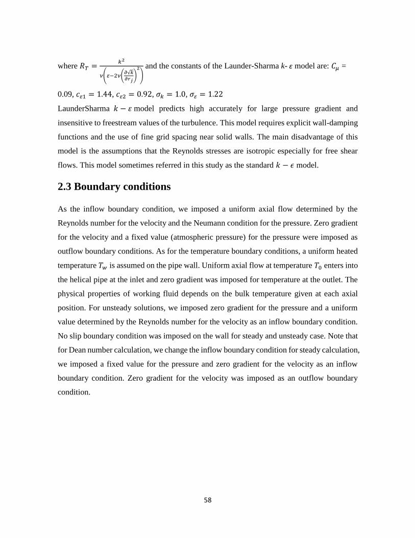
58

where 𝑅𝑇 =𝑘2

𝜈( −2𝜈(𝜕√𝑘

𝜕𝑟𝑗)

2

)

and the constants of the Launder-Sharma k- ԑ model are: 𝐶𝜇 =

0.09, 𝑐 1 = 1.44, 𝑐 2 = 0.92, 𝜎𝑘 = 1.0, 𝜎 = 1.22

LaunderSharma 𝑘 − 휀 model predicts high accurately for large pressure gradient and

insensitive to freestream values of the turbulence. This model requires explicit wall-damping

functions and the use of fine grid spacing near solid walls. The main disadvantage of this

model is the assumptions that the Reynolds stresses are isotropic especially for free shear

flows. This model sometimes referred in this study as the standard 𝑘 − 𝜖 model.

2.3 Boundary conditions

As the inflow boundary condition, we imposed a uniform axial flow determined by the

Reynolds number for the velocity and the Neumann condition for the pressure. Zero gradient

for the velocity and a fixed value (atmospheric pressure) for the pressure were imposed as

outflow boundary conditions. As for the temperature boundary conditions, a uniform heated

temperature 𝑇𝑤 is assumed on the pipe wall. Uniform axial flow at temperature 𝑇0 enters into

the helical pipe at the inlet and zero gradient was imposed for temperature at the outlet. The

physical properties of working fluid depends on the bulk temperature given at each axial

position. For unsteady solutions, we imposed zero gradient for the pressure and a uniform

value determined by the Reynolds number for the velocity as an inflow boundary condition.

No slip boundary condition was imposed on the wall for steady and unsteady case. Note that

for Dean number calculation, we change the inflow boundary condition for steady calculation,

we imposed a fixed value for the pressure and zero gradient for the velocity as an inflow

boundary condition. Zero gradient for the velocity was imposed as an outflow boundary

condition.

59

Chapter 3

3.1 Numerical Methods

3.2 Finite Volume Discretization

The purpose of any discretization method is to transform one or more partial differential

equations into a corresponding system of algebraic equations. The solution of this system

produces a set of values which correspond to the solution of the original equations at some

pre-determined locations in space and time, provided certain conditions, to be defined later,

and are satisfied. The discretization process can be divided into two steps: the discretization

of the solution domain and equation discretization.

The discretization of the solution domain produces a numerical description of the

computational domain, including the positions of points in which the solution is sought and

the description of the boundary. The space is divided into a finite number of discrete regions,

called control volumes or cells. For transient simulations, the time interval is also split into a

finite number of time-steps. Equation discretization gives an appropriate transformation of

terms of governing equations into algebraic expressions.

This Chapter presents the Finite Volume method (FVM) of discretization, with the following

properties:

The method is based on discretizing the integral form of governing equations over

each control volume. The basic quantities, such as mass and momentum, will

therefore be conserved at the discrete level.

Equations are solved in the fixed Cartesian coordinate system on the mesh that does

not change in time. The method is applicable to both steady-state and transient

calculations.

The control volumes can be of a general polyhedral shape, with a variable number of

neighbors, thus creating an arbitrarily unstructured mesh. All dependent variables

share the same control volumes, which is usually called the colocated or non-

staggered variable arrangement (Rhie and Chow (1982), Peric (1985)).

60

Systems of partial differential equations are treated in the different terminology way

(Patankar and Spalding (1972)), meaning that they are solved one at a time, with the

inter-equation coupling treated in the explicit manner. Non-linear differential

equations are linearized before the discretization and the non-linear terms are lagged.

The details of the discretization practice and implementation of boundary conditions will be

described in the remainder of this Chapter. In Section 3.2 the mesh arrangement is described.

Section 3.3 presents a discretization procedure for a scalar transport equation. The

discretization of the convection, diffusion and source terms is presented in section 3.3.1.1-

3.3.1.4. Several possibilities for the discretization of the temporal derivative are given in

Section 3.4. A new second order accurate and bounded convection differencing scheme and

some details of the solution procedure, including the treatment of mesh non-orthogonality,

deferred correction and the under-relaxation are given in Section 3.5. The solution procedure

for systems of partial differential equations and the generalized segregated approach for

pressure-velocity coupling is described in Section 3.6-3.7.

3.2.1 Discretization of the Solution Domain

Discretization of the solution domain produces a computational mesh on which the governing

equations are subsequently solved. It also determines the positions of points in space and

time where the solution is sought. The procedure can be split into two parts: discretization of

time and space.

61

Figure 3.1: Control volume (H. Jasak (1996))

Since time is a parabolic coordinate (Patankar (1981)), the solution is obtained by marching

in time from the prescribed initial condition. For the discretization of time, it is therefore

sufficient to prescribe the size of the time-step that will be used during the calculation. The

discretization of space for the finite volume method used in this study requires a subdivision

of the domain into control volumes (CV). Control volumes do not overlap and completely

fill the computational domain. In the present study all variables share the same control

volumes.

A typical control volume is shown in Fig. 3.1. The computational point P is located at the

centroid of the control volumes, such that:

∫ (𝑥 − 𝑥𝑝)𝑑𝑉 = 0.𝑉𝑝

(3.1)

The control volume is bounded by a set of flat faces and each face is shared with only one

neighboring control volume. The topology of the control volume is not important (it is a

general polyhedron).

62

The cell faces in the mesh can be divided into two groups - internal faces (between two

control volumes) and boundary faces, which coincide with the boundaries of the domain. The

face area vector 𝑆𝑓 is constructed for each face in such a way that it points outwards from the

cell with the lower label, is normal to the face and has the magnitude equal to the area of the

face. The cell with the lower label is called the “owner” of the face - its label is stored in the

“owner” array. The label of the other cell (“neighbor”) is stored in the “neighbor” array.

Boundary face area vectors point outwards from the computational domain - boundary faces

are “owned” by the adjacent cells. For the shaded face in Fig. 3.1, the owner and neighbor

cell centers are marked with P and N, as the face area vector 𝑆𝑓 points outwards from the P

control volume. For simplicity, all faces of the control volume will be marked with f, which

also represents the point in the middle of the face (see Fig. 3.1).

The capability of the discretization practice to deal with arbitrary control volumes gives

considerable freedom in mesh generation. It is particularly useful in meshing complex

geometrical configurations in three spatial dimensions. Arbitrarily unstructured meshes also

interact well with the concept of local grid refinement, where the computational points are

added in the parts of the domain where high resolution is necessary, without disturbing the

rest of the mesh.

3.3 Discretization of the Transport Equation

The standard form of the transport equation for a scalar property 𝜙 is:

𝜕𝜙

𝜕𝑡 + ∇. (𝑈𝜙) − ∇. (Γ𝜙∇𝜙) = 𝑆𝜙(𝜙) (3.2)

temporal derivative convection term diffusion term source term

Equation (3.2) is a second-order partial differential equation, as the diffusion term includes

the second derivative of 𝜙 in space. For good accuracy, it is necessary for the order of the

discretization to be equal to or higher than the order of the equation that is being discretized.

The individual terms of the transport equation will be treated separately.

63

In certain parts of the discretization it is necessary to relax the accuracy requirement, either

to accommodate the irregularities in the mesh structure or to preserve the boundedness of the

solution. Any deviation from the prescribed order of accuracy creates a discretization error,

which is of the order of other terms in the original equation and disappears only in the limit

of excessively mesh.

The accuracy of the discretization method depends on the assumed variation of the function

𝜙 = 𝜙 (x, t) in space and time around the point P. In order to obtain a second-order accurate

method, this variation must be linear in both space and time, i.e. it is assumed that:

𝜙(𝑥) = 𝜙𝑝 + (𝑥 − 𝑥𝑝). (∇𝜙)𝑝, (3.3)

𝜙(𝑡 + ∆𝑡) = 𝜙𝑡 + ∆𝑡 (𝜕𝜙

𝜕𝑡)𝑡

(3.4)

where

𝜙𝑝 = 𝜙(𝑥𝑝), (3.5)

𝜙𝑡 = 𝜙(𝑡). (3.6)

Let us consider the Taylor series expansion in space of a function around the point x:

𝜙(𝑥) = 𝜙𝑝 + (𝑥 − 𝑥𝑝). (∇𝜙)𝑝 +1

2(𝑥 − 𝑥𝑝)

2∶ (∇∇𝜙)𝑝 +

1

2!(𝑥 − 𝑥𝑝)

3∷ (∇∇∇𝜙)𝑝 +⋯+

1

𝑛!(𝑥 − 𝑥𝑝)

𝑛∷ (∇∇. . ∇𝜙)𝑝 +⋯ (3.7)

n n

In Eq. (3.7) consists the expression (𝑥 − 𝑥𝑝)𝑛

represents the nth tonsorial product of the

vector (𝑥 − 𝑥𝑝) with itself, producing an nth rank tensor. The operator “∷” is the inner

product of two nth rank tensors, creating a scalar.

Comparison between the assumed variation, Eq. (3.3), and the Taylor series expansion, Eqn.

(3.7), shows that the first term of the truncation error scales with |(𝑥 − 𝑥𝑝)2|, which is for a

1-D situation equal to the square of the size of the control volume. The assumed spatial

variation is therefore second-order accurate in space. An equivalent analysis shows that the

truncation error in Eqn. (3.4) scales with (∆𝑡)2 , resulting in the second-order temporal

accuracy.

64

The Finite Volume method requires that Eqn. (3.2) is satisfied over the control volume

𝑉𝑝 around the point P in the integral form:

∫ [𝜕

𝜕𝑡∫ 𝜙𝑑𝑉 +∫ ∇. (𝑈𝜙)𝑑𝑉 − ∫ ∇. (Γ𝜙∇𝜙)𝑑𝑉

𝑉𝑝𝑉𝑝𝑉𝑝

] 𝑑𝑡 = ∫ (∫ 𝑆𝜙(𝜙)𝑑𝑉𝑉𝑝

)𝑑𝑡𝑡+∆𝑡

𝑡

𝑡+∆𝑡

𝑡

(3.8)

The discretization of above equation will now be examined term by term.

3.3.1 Discretization of Spatial Terms

Let us first examine the discretization of spatial terms. The generalized form of Gauss'

theorem will be used throughout the discretization procedure, involving these identities:

∫ ∇. 𝑎 𝑑𝑉 = ∮ 𝑑𝑆. 𝑎,𝜕𝑉𝑉

(3.9)

∫ ∇𝜙 𝑑𝑉 = ∮ 𝑑𝑆𝜙,𝜕𝑉𝑉

(3.10)

∫ ∇𝑎 𝑑𝑉 = ∮ 𝑑𝑆𝑎, (3.11)𝜕𝑉𝑉

where 𝜕𝑉 si the closed surface bounding the volume V and dS represents an infinitesimal

surface element with associated outward pointing normal on 𝜕𝑉.

A series of volume and surface integrals needs to be evaluated. Taking into account the

prescribed variation of 𝜙 over the control volume P, Eq. (3.3), it follows:

∫ 𝜙(𝑥)𝑑𝑉 = ∫ [𝜙𝑝 + (𝑥 − 𝑥𝑝). (∇𝜙)𝑝]𝑑𝑉𝑉𝑝𝑉𝑝

= 𝜙𝑝 ∫ 𝑑𝑉 + [∫ (𝑥 − 𝑥𝑝)𝑑𝑉𝑉𝑝] .

𝑉𝑝(∇𝜙)𝑝

= 𝜙𝑝𝑉𝑝 (3.12)

where 𝑉𝑝 is the volume of the cell. The second integral in Eq. (3.12) is equal to zero because

the point P is the centroid of the control volume.

Let us now consider the terms under the divergence operator. Having in mind that the control

volume is bounded by a series of flat faces, Eq. (3.9) can be transformed into a sum of

integrals over all faces:

65

∫ ∇. 𝑎 𝑑𝑉 = ∮ 𝑑𝑆. 𝑎𝜕𝑉𝑝𝑉

= ∑(∫ 𝑑𝑆. 𝑎𝑓

). (3.13)

𝑓

The assumption of linear variation of 𝜙 leads to the following expression for the face integral

in Eqn. (3.13):

∮ 𝑑𝑆. 𝑎𝑓

= 𝑆. 𝑎𝑓 . (3.14)

Combining Eqs. 3.12, 3.13 and 3.14, a second-order accurate discretized form of the Gauss'

theorem is obtained:

(∇. 𝑎) 𝑉𝑝 =∑𝑆. 𝑎𝑓𝑓

(3.15)

Here, the subscript f implies the value of the variable (in this case, a) in the middle of the

face and S is the outward-pointing face area vector. In the current mesh structure, the face

area vector 𝑆𝑓 point outwards from P only if f is “owned” by P. For the “neighboring” faces

𝑆𝑓 points inwards, which needs to be taken into account in the sum in Eq. (3.15). The sum

over the faces is therefore split into sums over “owned” and “neighboring” faces:

∑𝑆. 𝑎𝑓𝑓

= ∑ 𝑆𝑓 . 𝑎𝑓𝑜𝑤𝑛𝑒𝑟

− ∑ 𝑆𝑓 . 𝑎𝑓𝑛𝑒𝑖𝑔ℎ𝑏𝑜𝑢𝑟

. (3.16)

This is true for every summation over the faces. In the rest of the text, this split is

automatically assumed.

3.3.1.1 Convection Term

The discretization of the convection term is obtained using Eq. (3.15):

∫ ∇. (𝑈𝜙) 𝑑𝑉 =∑𝑆. (𝑈𝜙)𝑓𝑓𝑉𝑝

= ∑𝑆

𝑓

. (𝑈)𝑓𝜙𝑓

= ∑𝐹

𝑓

𝜙𝑓 (3.17)

66

where F in Eq. (3.17) represents the mass flux through the face

𝐹 = 𝑺. (𝑈)𝑓 (3.18)

Equations (3.17 and 3.18) also require the face value of the variable 𝜙 calculated from the

values in the cell centers, which is obtained using the convection differencing scheme.

Before we continue the formulation of the convection differencing scheme, it is necessary to

examine the physical properties of the convection term. Irrespective of the distribution of the

velocity in the domain, the convection term does not violate the bounds of 𝜙 given by its

initial distribution. If, for example, 𝜙 initially varies between 0 and 1, the convection term

will never produce the values of 𝜙 that are lower than zero or higher than unity. Considering

the importance of boundedness in the transport of scalar properties of interest, it is essential

to preserve this property in the discretized form of the term.

3.3.1.2 Convection Differencing Scheme

The role of the convection differencing scheme is to determine the value of 𝜙 on the face

from the values in the cell centers. In the framework of arbitrarily unstructured meshes, it

would be impractical to use any values other than 𝜙𝑃 and 𝜙𝑁 , because of the storage

overhead associated with the additional addressing information. We shall therefore limit

ourselves to differencing schemes using only the nearest neighbors of the control volume.

Fig. 3.2 Face interpolation

Assuming the linear variation of 𝜙 between P and N, Fig. 3.2, the face value is calculated

according to:

𝜙𝑓 = 𝑓𝑥𝜙𝑃 + (1 − 𝑓𝑥)𝜙𝑁 . (3.19)

Here, the interpolation factor 𝑓𝑥 is defined as the ratio of distances 𝑓𝑁 and 𝑃𝑁:

67

𝑓𝑥 =𝑓𝑁

𝑃𝑁. (3.20)

The differencing scheme using Eqn. (3.19) to determine the face value of 𝜙 is called central

differencing (CD). Although this has been the subject of some debate, Ferziger and Peric

(1995) show that it is second order accurate even on non- uniform meshes. This is consistent

with the overall accuracy of the method. It has been noted, however, that CD causes

unphysical oscillations in the solution for convection-dominated problems (Patankar, (1972)),

thus violating the boundedness of the solution.

An alternative discretization scheme that guarantees boundedness is upwind differencing

(UD). The face value of 𝜙 is determined according to the direction of the flow:

𝜙𝑓 = {𝜙𝑓 = 𝜙𝑃 for 𝐹 ≥ 0

𝜙𝑓 = 𝜙𝑁 for 𝐹 < 0 (3.21)

Boundedness of the solution is guaranteed through the sufficient boundedness criterion for

systems of algebraic equations (see e.g. Patankar, (1972)). Boundedness of UD is effectively

insured at the expense of the accuracy, by implicitly introducing the numerical diffusion term.

This term violates the order of accuracy of the discretization and can severely distort the

solution.

Blended Differencing (BD) (Peric (1985)) represents an attempt to preserve both

boundedness and accuracy of the solution. It is a linear combination of upwind differencing,

Eqn. (3.21) and central differencing, Eqn. (3.19):

𝜙𝑓 = 𝛾(𝜙𝑓)𝐶𝐷+ (1 − 𝛾)(𝜙𝑓)𝑈𝐷

, (3.22)

The blending factor 𝛾 , 0 ≤ 𝛾 ≤ 1, determines how much numerical diffusion will be

introduced. Peric (1985) proposes a constant 𝛾 for all faces of the mesh. For 𝛾 = 0 the scheme

reduces to UD. The most promising approach at this stage combines a higher-order scheme

with upwind differencing on a face-by- face basis, based on different boundedness criteria.

68

3.3.1.3 Diffusion Term

The diffusion term will be discretized in a similar way. Using the assumption of linear

variation of 𝜙 and Eqn. (3.15), it follows:

∫ ∇. (Γ𝜙∇𝜙)𝑑𝑉 =∑𝑺.

𝑓𝑉𝑝

(Γ𝜙∇𝜙)𝑓

= ∑ (Γ𝜙)𝑓𝑺𝑓 . (∇𝜙)𝑓 (3.23)

If the mesh is orthogonal, i.e. vectors d and S in Fig. 3.3 are parallel, it is possible

Fig. 3.3 Vector d and S on a non-orthogonal mesh

to use the following expression:

𝑺. (∇𝜙)𝑓 = |𝑆| 𝜙𝑁−𝜙𝑃

|𝑑|. (3.24)

Using Eqn. (3.24), the face gradient of 𝜙 can be calculated from the two values around the

face. An alternative would be to calculate the cell-centred gradient for the two cells sharing

the face as:

(∇𝜙)𝑃 =1

𝑉𝑝∑ 𝑺𝑓 𝜙𝑓 , (3.25)

interpolate it to the face:

(∇𝜙)𝑓 = 𝑓𝑥(∇𝜙)𝑃 + (1 − 𝑓𝑥)(∇𝜙)𝑁. (3.26)

Although both of the above-described methods are second-order accurate, Eqn. (3.26) uses a

larger computational module. The first term of the truncation error is now four times larger

than in the first method, which in turn cannot be used on non-orthogonal meshes.

In order to make use of the higher accuracy of Eqn. (3.24), the product 𝑺. (∇𝜙)𝑓) is split into

two parts:

69

𝑺. (∇𝜙)𝑓 = ∆. (∇𝜙)𝑓 + 𝒌. (∇𝜙)𝑓 (3.27)

Orthogonal contribution non-orthogonal correction

The two vectors introduced in Eq. (3.27), ∆ and k, have got to satisfy the following condition:

𝑺 = ∆ + 𝒌

Vectors ∆ is chosen to be parallel with d. This allows us to use Eqn. (3.24) on the orthogonal

contribution, limiting the less accurate method only to the non- orthogonal part which cannot

be treated in any other way.

Orthogonal correction approach. This approach keeps the contribution from 𝜙𝑃 and 𝜙𝑁the

same as on the orthogonal mesh irrespective of the non- orthogonality, Fig. 3.4. To achieve

this we define:

∆ =𝒅

|𝒅||𝑺| (3.28)

Fig.3.4 Non-orthogonality treatment in the “orthogonal correction” approach

The diffusion term, Eq. (3.24), in its differential form exhibits the bounded behavior. Its

discretized form will preserve this property only on orthogonal meshes. The non-orthogonal

correction potentially creates unboundedness, particularly if mesh non-orthogonality is high.

If the preservation of boundedness is more important than accuracy, the non-orthogonal

correction has got to be limited or completely discarded, thus violating the order of accuracy

of the discretization.

3.3.1.4 Source Terms

All terms of the original equation that cannot be written as convection, diffusion or temporal

terms are treated as sources. The source term, 𝑆𝜙(𝜙), can be a general function of 𝜙. When

deciding on the form of the discretization for the source, its interaction with other terms in

the equation and its influence on boundedness and accuracy should be examined. Some

70

general comments on the treatment of source terms are given in Patankar (1972). A simple

procedure will be explained here.

Before the actual discretization, the source term needs to be linearized:

𝑆𝜙(𝜙) = 𝑆𝑢 + 𝑆𝑝𝜙, (3.29)

where Su and Sp can also depend on 𝜙 . Following Eq. (3.12), the volume integral is

calculated as:

∫ 𝑆𝜙(𝜙)𝑑𝑉 = 𝑆𝑢𝑉𝑝 + 𝑆𝑝𝑉𝑝𝑉𝑝𝜙𝑝 (3.30)

The importance of the linearization becomes clear in implicit calculations. It is desirable to

treat the source term as “implicitly” as possible.

3.4 Temporal discretization In the previous Section, the discretization of spatial terms has been presented. This can be

split into two parts, the transformation of surface and volume integrals into discrete sums and

expressions that give the face values of the variable as a function of cell values. Let us again

consider the integral form of the transport equation:

∫ [𝜕

𝜕𝑡∫ 𝜙𝑑𝑉 +∫ ∇. (𝑈𝜙)𝑑𝑉 − ∫ ∇. (Γ𝜙∇𝜙)𝑑𝑉

𝑉𝑝𝑉𝑝𝑉𝑝

] 𝑑𝑡 = ∫ (∫ 𝑆𝜙(𝜙)𝑑𝑉𝑉𝑝

)𝑑𝑡𝑡+∆𝑡

𝑡

𝑡+∆𝑡

𝑡

(3.31)

Using Eqns. 3.17 and 3.30, and assuming that the control volumes do not change in time, so,

transport equation can be written as:

∫ [(𝜕𝜙

𝜕𝑡)𝑃𝑉𝑝 +∑𝐹𝜙𝑓 −∑(Γ𝜙)𝑓

𝑆. (∇𝜙)𝑓𝑓𝑓

] 𝑑𝑡 = ∫ (𝑆𝑢𝑉𝑝 + 𝑆𝑝𝑉𝑝𝜙𝑝)𝑑𝑡 (3.32)𝑡+∆𝑡

𝑡

𝑡+∆𝑡

𝑡

The above expression is usually called the “semi-discretized” form of the transport equation.

Having in mind the prescribed variation of the function in time, Eq. (3.32), the temporal

integrals and the time derivative can be calculated directly as:

(𝜕𝜙

𝜕𝑡)𝑃=

𝜙𝑃𝑛−𝜙𝑃

0

∆𝑡, (3.33)

∫ 𝜙(𝑡)𝑑𝑡 =1

2

𝑡+∆𝑡

𝑡(𝜙0 + 𝜙𝑛) ∆𝑡, (3.34)

where

𝜙𝑛 = 𝜙(𝑡 + ∆𝑡), (3.35)

71

𝜙0 = 𝜙(𝑡). (3.36)

Assuming that the density and diffusivity do not change in time, Eqs. 3.32, 3.32 and 3.34

give:

𝑃𝜙𝑃𝑛 − 𝑃𝜙𝑃

0

∆𝑡𝑉𝑝 +

1

2∑𝐹𝜙𝑓

𝑛 −1

2∑(Γ𝜙)𝑓

𝑆. (∇𝜙)𝑓𝑛

𝑓𝑓

+1

2∑𝐹𝜙𝑓

0 −1

2∑(Γ𝜙)𝑓

𝑆. (∇𝜙)𝑓0 = 𝑆𝑢𝑉𝑝 +

1

2𝑆𝑝𝑉𝑝𝜙𝑃

𝑛

𝑓𝑓

+1

2𝑆𝑝𝑉𝑝𝜙𝑃

0 .

(3.37)

This form of temporal discretization is called the Crank-Nicholson method. It is second-order

accurate in time. It requires the face values of 𝜙 and ∇𝜙 as well as the cell values for both

old and new time-step. The face values are calculated from the cell values on each side of the

face, using the appropriate differencing scheme for the convection term. Our task is to

determine the new value of 𝜙𝑝 . Since 𝜙𝑓 and (∇𝜙)𝑓 also depend on values of 𝜙 in the

surrounding cells, Eq. (3.37) is reduced to an algebraic equation:

𝑎𝑝𝜙𝑃𝑛 +∑𝑎𝑁𝜙𝑁

𝑛 = 𝑅𝑝 (3.38)

𝑁

For every control volume, an equation of this form is assembled. The value of 𝜙𝑃𝑛

depends

on the values in the neighboring cells, thus creating a system of algebraic equations:

[𝐴][𝜙] = [𝑅], (3.39)

where [A] is a sparse matrix, with coefficients 𝑎𝑝 on the diagonal and 𝑎𝑁 off the diagonal,

[𝜙] is the vector of 𝜙-s for all control volumes and [R] is the source term vector. The

sparseness pattern of the matrix depends on the order in which the control volumes are

labelled, with every off-diagonal coefficient above and below the diagonal corresponding to

one of the faces in the mesh. In the rest of this study, Eq. (3.39) will be represented by the

typical equation for the control volume, Eq. (3.38).

When this system is solved, it gives a new set of 𝜙 values, the solution for the new time-step.

As will be shown later, the coefficient 𝑎𝑝 in Eq. (3.38) includes the contribution from all

terms corresponding to 𝜙𝑃𝑛, the temporal derivative, convection and diffusion terms as well

as the linear part of the source term. The coefficients 𝑎𝑁 include the corresponding terms for

each of the neighboring points. The summation is done over all CVs that share a face with

72

the current control volume. The source term includes all terms that can be evaluated without

knowing the new 𝜙 , namely, the constant part of the source term, and the parts of the

temporal derivative, convection and diffusion terms corresponding to the old time- level.

The Crank-Nicholson method of temporal discretization is unconditionally stable, but does

not guarantee boundedness of the solution. Examples of unrealistic solutions given by the

Crank-Nicholson scheme can be found in Patankar and Baliga (1978). As in the case of the

convection term, boundedness can be obtained if the equation is discretized to first order

temporal accuracy.

It has been customary neglected the variation of the face values of 𝜙 and ∇𝜙 in time

(Patankar (1972)). This leads to several methods of temporal discretization. The new form of

the discretized transport equation combines the old and new time-step convection, diffusion

and source terms, leaving the temporal derivative unchanged:

𝜙𝑃𝑛 − 𝜙𝑃

0

∆𝑡𝑉𝑝 +∑𝐹𝜙𝑓 −∑(Γ𝜙)𝑓

𝑆. (∇𝜙)𝑓𝑓𝑓

= 𝑆𝑢𝑉𝑃 + 𝑆𝑝𝑉𝑃𝜙𝑃 (3.40)

The resulting equation is only first-order accurate in time and a choice has to be made about

the way the face values of 𝜙 and ∇𝜙 are evaluated.

In explicit discretization, the face values of 𝜙 and ∇𝜙 are determined from the old-time field:

𝜙𝑓 = 𝑓𝑥𝜙𝑃0 + (1 − 𝑓𝑥)𝜙𝑁

0 , (3.41)

𝑺. (∇𝜙)𝑓 = |∆| 𝜙𝑁0 −𝜙𝑃

0

|𝑑|+ 𝒌. (∇𝜙)𝑓

0 (3.42)

The linear part of the source term is also evaluated using the old-time value. Eq. (3.44) can

be written in the form:

𝜙𝑃𝑛 = 𝜙𝑃

0 +∆𝑡

𝑉𝑝[∑𝐹𝜙𝑓 −∑(Γ𝜙)𝑓

𝑺. (∇𝜙)𝑓𝑓𝑓

= 𝑆𝑢𝑉𝑃 + 𝑆𝑝𝑉𝑃𝜙𝑃0]. (3.43)

The consequence of this choice is that all terms on the r.h.s. of Eq. (3.43) depend only on the

old-time field. The new value of 𝜙𝑃 can be calculated directly - it is no longer necessary to

solve the system of linear equations. The drawback of this method is the Courant number

limit (Courant et al. (1928)). The Courant number is defined as:

𝐶0 =𝑈𝑓.𝑑

∆𝑡. (3.44)

73

If the Courant number is larger than unity, the explicit system becomes unstable. This is a

severe limitation, especially if we are trying to solve a steady-state problem.

3.5 Solution techniques

Let us again consider the system of algebraic equations created by the discretization, Eq.

(3.42):

𝑎𝑝𝜙𝑃𝑛 +∑𝑎𝑁𝜙𝑁

𝑛 = 𝑅𝑝 (3.45)

𝑁

This system can be solved in several different ways. Existing solution algorithms are

classified into two main categories: direct and iterative methods. Direct methods give the

solution of the system of algebraic equations in a finite number of arithmetic operations.

Iterative methods start with an initial guess and then continue to improve the current

approximation of the solution until some “solution tolerance” is met. While direct methods

are appropriate for small systems, the number of operations necessary to reach the solution

raises with the number of equations, making them prohibitively expensive for large systems.

Iterative methods are more economical, but they usually pose some requirements on the

matrix.

The matrix resulting from Eq. (3.38) is sparse-most of the matrix coefficients are equal to

zero. If it were possible to choose a solver which preserves the sparsity pattern of the matrix,

the computer memory requirements would be significantly decreased. Unlike direct solvers,

some iterative methods preserve the sparseness of the original matrix. These properties make

the use of iterative solvers very attractive.

Iterative solvers require diagonal dominance in order to guarantee convergence. A matrix is

said to be diagonally equal if the magnitude of the diagonal coefficient is equal to the sum of

magnitudes of off-diagonal coefficients. The additional condition for diagonal dominance is

|𝑎𝑃| > ∑ |𝑎𝑁|𝑛 for at least one row of the matrix.

In order to improve the solver convergence, it is desirable to increase the diagonal dominance

of the system. Discretization of the linear part of the source term, Eq. (3.32), is closely related

74

to this issue. If 𝑆𝑝< 0, its contribution increases diagonal dominance and 𝑆𝑝 is included into

the diagonal. In the case of 𝑆𝑝 > 0, diagonal dominance would be decreased. It is more

effective to include this term into the source and update it when the new solution is obtained.

This measure is, however, not sufficient to guarantee the diagonal dominance of the matrix.

The analysis of the structure of the matrix leads us back to the issue of boundedness. The

sufficient boundedness criterion for systems of algebraic equations mentioned states that the

boundedness of the solution will be preserved for diagonally equal systems of equations with

positive coefficients. This allows us to examine the discretized form of all the terms in the

transport equation from the point of view of boundedness and diagonal dominance and

identify the troublesome parts of discretization.

The convection term creates a diagonally equal matrix only for upwind differencing. Any

other differencing scheme will create negative coefficients, violate the diagonal equality and

potentially create unbounded solutions. In the case of central differencing on a uniform mesh,

the problem is further complicated by the fact that the central coefficient is equal to zero. In

order to improve the quality of the matrix for higher-order differencing schemes, Khosla and

Rubin (1974) propose a correction implementation for the convection term. Here, any

differencing scheme is treated as an upgrade of upwind differencing. The part of the

convection term corresponding to upwind differencing is treated implicitly (i.e. built into the

matrix) and the other part is added into the source term. This, however, does not affect the

boundedness in spite of the fact that the matrix is now diagonally equal, as the “troublesome”

part of the discretization still exists in the source term.

The diffusion term creates a diagonally equal matrix only if the mesh is orthogonal. On non-

orthogonal meshes, introduces the “second neighbors” of the control volume into the

computational molecule with negative coefficients, thus violating diagonal equality. As a

consequence of mesh non-orthogonality, the boundedness of the solution cannot be

guaranteed. The increase in the computational molecule would result in a higher number of

non-zero matrix coefficients, implying a considerable increase in the computational effort

75

required to solve the system. On the other hand, the non-orthogonal correction is usually

small compared to the implicit part of the diffusion term. It is therefore reasonable to treat it

through the source term. In this study, the diffusion term will therefore be split into the

implicit orthogonal contribution, which includes only the first neighbors of the cell and

creates a diagonally equal matrix and the non- orthogonal correction, which will be added to

the source. If it is important to resolve the non-orthogonal parts of the diffusion operators

(like in the case of the pressure equation), non-orthogonal correctors are included. The system

of algebraic equations, Eqn. (3.38), will be solved several times. Each new solution will be

used to update the non-orthogonal correction terms, until the desired tolerance is obtained. It

should again be noted that this practice only improves the quality of the matrix but does not

guarantee boundedness. If boundedness is essential, the non-orthogonal contribution should

be discarded.

The decomposition of the face area vector into the orthogonal and non-orthogonal part

determines the split between the implicit and explicit part of the term, with the consequences

on the accuracy and convergence of non-orthogonal correctors. The comparison of different

treatments is based on several criteria:

It is necessary to introduce non-orthogonal correctors - how good an approximation

of the converged solution can be obtained after only one solution of the system?

How many non-orthogonal correctors are needed to meet a certain tolerance?

How does the number of solver iterations change with the number of correctors?

If the non-orthogonal correction needs to be discarded for the sake of boundedness,

which approach causes the smallest discretization error?

The discretization of the temporal derivative creates only the diagonal coefficient and a

source term contribution, thus increasing the diagonal dominance. Unfortunately, the

sufficient boundedness criterion cannot be used to establish the boundedness of the

discretization, as it does not take into account the influence of the source term.

The above discussion is concentrated on the analysis of the discretization on a term- by-term

basis. In reality, all of the above coefficients contribute to the matrix, thus influencing the

properties of the system. It has been shown that the only terms that actually enhance the

diagonal dominance are the linear part of the source and the temporal derivative.

76

In steady-state calculations, the beneficial influence of the temporal derivative on the

diagonal dominance does not exist. In order to enable the use iterative solvers, the diagonal

dominance needs to be enhanced in some other way, namely through under-relaxation.

Consider the original system of equations, Eq. (3.38):

𝑎𝑝𝜙𝑃𝑛 + ∑ 𝑎𝑁𝜙𝑁

𝑛 = 𝑅𝑝𝑁 , (3.46)

Diagonal dominance is achieved by an artificial term added to both left and right-hand side

of Eqn. (3.38):

𝑎𝑝𝜙𝑃𝑛 +

1 − 𝛼

𝛼𝑎𝑝𝜙𝑃

𝑛 +∑𝑎𝑁𝜙𝑁𝑛 = 𝑅𝑝

𝑁

+1 − 𝛼


0 (3.47)

or

𝑎𝑝𝜙𝑃

𝑛

𝛼+∑𝑎𝑁𝜙𝑁

𝑛 = 𝑅𝑝𝑁

+1 − 𝛼


0 (3.48)

𝜙𝑃0 here represents the value of 𝜙 from the previous iteration and 𝛼 is the under-relaxation

factor (0 < 𝛼 < 1). Additional terms cancel out when steady-state is reached (𝜙𝑃0 = 𝜙𝑃

𝑛)

In present study, the iterative solution procedure used to solve the system of algebraic

equations is the conjugate gradient (CG) method, originally proposed by Hestens and Steifel

(1952). It guarantees that the exact solution will be obtained in the number of iterations

smaller or equal to the number of equations in the system. The convergence rate of the solver

depends on the dispersion of the eigenvalues of the matrix [A] in Eq. (3.39) and can be

improved through pre-conditioning. For symmetric matrices, the incomplete cholesky

preconditioned conjugate gradient (ICCG) solver will be used. The method is described in

detail by Jacobs(1980).

3.6 Discretization procedure for the Navier-Stokes system

In this Section, a discretization procedure for the Navier-Stokes equations will be presented.

We shall start with the incompressible form of the system, Eqns. (2.1 and 2.2):

𝛻 ∙ 𝑼 = 0, (3.49)

77

𝜕𝑼

𝜕𝑡+ (𝑼 ∙ 𝛻)𝑼 = −

1

𝜌𝛻𝑝 + 𝜈𝛻2𝑼. (3.50)

Two issues require special attention: non-linearity of the momentum equation and the

pressure-velocity coupling.

The non-linear term in Eq. (2.1) is (𝑼 ∙ 𝛻)𝑼, i.e. velocity is “being transported by itself”. The

discretized form of this expression would be quadratic in velocity and the resulting system

of algebraic equations would therefore be non-linear. There are two possible solutions for

this problem - either use a solver for non-linear systems, or linearize the convection term.

(𝑼 ∙ 𝛻)𝑼 = ∑ 𝑺. (𝑼)𝑓𝑓 (𝑼)𝑓 = ∑ 𝐹𝑓 (𝑼)𝑓,

= 𝑎𝑃𝑈𝑃 + ∑ 𝑎𝑁𝑈𝑁𝑁 , (3.51)

where F, 𝑎𝑃 and 𝑎𝑁 are a function of U. The important issue is that the fluxes F should satisfy

the continuity equation, Eqn. 2.1 and 2.2 should therefore be solved together, resulting in an

even larger (non-linear) system. Having in mind the complexity of nonlinear equation solvers

and the computational effort required, linearization of the term is preferred. Linearization of

the convection term implies that an existing velocity (flux) field that satisfies Eq. (2.1) will

be used to calculate 𝑎𝑃 and 𝑎𝑁.

The linearization does not have any effect in steady-state calculations. When the steady-state

is reached, the fact that a part of the nonlinear term has been lagged is not significant. In

transient flows two different approaches can be adopted: either to iterate over non-linear

terms or to neglect the lagged nonlinearity effects. Iteration can significantly increase the

computational cost, but only if the time-step is large. The advantage is that the nonlinear

system is fully resolved for every time-step, whose size limitation comes only from the

temporal accuracy requirements. If it is necessary to resolve the temporal behavior well, a

small time-step is needed. On the other hand, if the time-step is small, the change between

consecutive solutions will also be small and it is therefore possible to lag the nonlinearity

without any significant effect.

In this study, the PISO procedure proposed by Issa (1986) is used for pressure-velocity

coupling in transient calculations. For steady-state calculations, a SIMPLE pressure-velocity

coupling procedure by Patankar (1972) is used.

78

In Section 3.6.1 the problem of pressure-velocity coupling is presented. The pressure

equation is derived for the incompressible Navier-Stokes equations. Section 3.6.2 describes

the pressure-velocity coupling algorithms.

3.6.1 Derivation of the pressure equation

In order to derive the pressure equation, a semi-discretized form of the momentum equation

is used:

𝑎𝑃𝑈𝑃 = 𝑯(𝑼) − ∇𝑝. (3.52)

In the spirit procedure of the Rhie and Chow (1982), the pressure gradient term is not

discretized at this stage. Eq. 3.52 is obtained from the integral form of the momentum

equation, using the discretization procedure described previously. It has been consequently

divided through by the volume in order to enable face interpolation of the coefficients.

The 𝑯(𝑼) term consists of two parts: the “transport part”, including the matrix coefficients

for all neighbors multiplied by corresponding velocities and the “source part” including the

source part of the transient term and all other source terms apart from the pressure gradient

(in our case, there is no additional source terms):

𝑯(𝑼) = −∑ 𝑎𝑁𝑈𝑁𝑁 +𝑼0

∆𝑡. (3.53)

The discretized form of the continuity equation (Eqn. 2.23) is:

∇.𝑼 = ∑ 𝑺.𝑈𝑓 = 0𝑓 . (3.54)

Eqn. (3.52) is used to express U:

𝑈𝑃 =𝑯(𝑼)

𝑎𝑃−

1

𝑎𝑃∇𝑃. (3.55)

Velocities on the cell face are expressed as the face interpolate of Eqn. 3.55:

𝑈𝑓 = (𝑯(𝑼)

𝑎𝑃)𝑓− (

1

𝑎𝑃)𝑓(∇𝑃)𝑓. (3.56)

This will be used later to calculate the face fluxes.

When Eq. (3.56) is substituted into Eqn. 3.54, the following form of the pressure equation is

obtained:

∇. (∇𝑃

𝑎𝑃) = ∇. (

𝑯(𝑼)

𝑎𝑃) = ∑ 𝑺. (

𝑯(𝑼)

𝑎𝑃)𝑓

𝑓 . (3.57)

The Laplacian on the L.H.S. of Eqn. 3.57 is discretized in the standard way.

79

The final form of the discretized incompressible Navier-Stokes system is:

𝑎𝑃𝑈𝑃 = 𝑯(𝑼) − ∑ 𝑺(𝑝)𝑓𝑓 , (3.58)

∑ 𝑺. [(1

𝑎𝑃)𝑓(∇𝑝)𝑓]𝑓 = ∑ 𝑺. (

𝑯(𝑼)

𝑎𝑃)𝑓

𝑓 . (3.59)

The face flux F is calculated using Eqn. 3.56:

𝐹 = 𝑺.𝑈𝑓 = 𝑺. [(𝑯(𝑼)

𝑎𝑃)𝑓− (

1

𝑎𝑃)𝑓(∇𝑝)𝑓]. (3.60)

When Eq. (3.141) is satisfied, the face fluxes are guaranteed to be conservative.

3.6.2 Pressure-velocity coupling

Consider the discretized form of the Navier-Stokes (Eqns. 3.58 and 3.59). The form of the

equations shows linear dependence of velocity on pressure and vice-versa. Simultaneous

algorithms operate by solving the complete system of equations simultaneously over the

whole domain. Such a procedure might be considered when the number of computational

points is small and the number of simultaneous equations is not too large. The resulting

matrix includes the inter-equation coupling and is several times larger than the number of

computational points. The cost of a simultaneous solution is great, both in the number of

operations and memory requirements.

A special treatment is required in order to establish the necessary inter-equation coupling.

PISO (Issa (1986)), SIMPLE (Patankar (1972)), and their derivatives are the most popular

methods of dealing with inter-equation coupling in the pressure-velocity system.

3.8.2.1 The PISO algorithm for transient flows

This pressure-velocity treatment for transient flow calculations has been originally proposed

by Issa (1986). Let us again consider the discretized Navier-Stokes equations for

incompressible flow, (Eqns. 3.58 and 3.59). The PISO algorithm can be described as follows:

The momentum equation is solved first. The exact pressure gradient source term is

not known at this stage - the pressure field from the previous time-step is used instead.

80

This stage is called the momentum predictor. The solution of the momentum equation,

Eq. (3.58) gives an approximation of the new velocity field.

Using the predicted velocities, the H(U) operator can be assembled and the pressure

equation can be formulated. The solution of the pressure equation gives the first

estimate of the new pressure field. This step is called the pressure solution.

Eqn. 3.60 gives a set of conservative fluxes consistent with the new pressure field.

The velocity field should also be corrected as a consequence of the new pressure

distribution. Velocity correction is done in an explicit manner, using Eqn. 3.55). This

is the explicit velocity correction stage.

A closer look to Eqn. 3.55 reveals that the velocity correction actually consists of two parts

- a correction due to the change in the pressure gradient (∇𝑝 𝑎𝑃⁄ term) and the transported

influence of corrections of neighboring velocities (𝑯(𝑼) 𝑎𝑃⁄ term). The fact that the velocity

correction is explicit means that the latter part is neglected - it is effectively assumed that the

whole velocity error comes from the error in the pressure term. This, of course, is not true. It

is therefore necessary to correct the H(U) term to formulate the new pressure equation and

repeat the procedure. In other words, the PISO loop consists of an implicit momentum

predictor followed by a series of pressure solutions and explicit velocity corrections. The

loop is repeated until a pre-determined tolerance is reached.

Another issue is the dependence of H(U) coefficients on the flux field. After each pressure

solution, a new set of conservative fluxes is available. It would be therefore possible to

recalculate the coefficients in H(U). This, however, is not done: it is assumed that the non-

linear coupling is less important than the pressure-velocity coupling, consistent with the

linearization of the momentum equation. The coefficients in H(U) are therefore kept constant

through the whole correction sequence and will be changed only in the next momentum

predictor.

3.6.2.2 The SIMPLE algorithm

If a steady-state problem is being solved iteratively, it is not necessary to fully resolve the

linear pressure-velocity coupling, as the changes between consecutive solutions are no longer

81

small. Nonlinearity of the system becomes more important, since the effective time-step is

much larger.

The SIMPLE algorithm by Patankar (1981) is formulated to take advantage of these facts:

An approximation of the velocity field is obtained by solving the momentum equation.

The pressure gradient term is calculated using the pressure distribution from the

previous iteration or an initial guess. The equation is under-relaxed in an implicit

manner, with the velocity under-relaxation factor 𝛼𝑈.

The pressure equation is formulated and solved in order to obtain the new pressure

distribution.

A new set of conservative fluxes is calculated using Eqn. 3.60. As it has been noticed

before, the new pressure field includes both the pressure error and convection-

diffusion error. In order to obtain a better approximation of the “correct” pressure

field, it is necessary to solve the pressure equation again. On the other hand, the non-

linear effects are more important than in the case of transient calculations. It is enough

to obtain an approximation of the pressure field and recalculate the H(U) coefficients

with the new set of conservative fluxes. The pressure solution is therefore under-

relaxed in order to take into account of the velocity part of the error:

𝑝𝑛𝑒𝑤 = 𝑝𝑜𝑙𝑑 + 𝛼𝑝(𝑝𝑝 − 𝑝𝑜𝑙𝑑) (3.61)

where

- 𝑝𝑛𝑒𝑤 is the approximation of the pressure field that will be used in the next momentum

predictor,

- 𝑝𝑜𝑙𝑑 is the pressure field used in the momentum predictor,

- 𝑝𝑝is the solution of the pressure equation,

-𝛼𝑝 is the pressure under-relaxation factor, (0 < 𝛼𝑝 < 1).

If the velocities are needed before the next momentum solution is obtained, the explicit

velocity correction, Eqn. 3.55, is performed.

82

Peric(1985) gives an analysis of the under-relaxation procedure based on the expected

behavior of the second corrector in the PISO sequence. The recommended values of under-

relaxation factors are (Peric(1985):

𝛼𝑝 = 0.2 for the pressure

𝛼𝑝 = 0.8 for momentum.

3.7 Solution procedure for the Navier-Stokes equations

It is now possible to describe the solution sequence for the Navier-Stokes system with

additional coupled transport equations (e.g. a turbulence model, energy equation or some

other equations that influence the system).

In transient calculations, all inter-equation couplings apart from the pressure- velocity system

are lagged. If it is necessary to ensure a closer coupling between some of the equations (e.g.

energy and pressure in combustion), they are included in the PISO loop. A transient solution

procedure for incompressible turbulent flows can be summarized as follows:

1. Set up the initial conditions for all field values.

2. Start the calculation of the new time-step values.

3. Assemble and solve the momentum predictor equation with the available face fluxes.

4. Go through the PISO loop until the tolerance for pressure-velocity system is reached.

At this stage, pressure and velocity fields for the current time-step are obtained, as

well as the new set of conservative fluxes.

5. Using the conservative fluxes, solve all other equations in the system. If the flow is

turbulent, calculate the effective viscosity from the turbulence variables.

6. If the final time is not reached, return to step 2.

The solution procedure for steady-state incompressible turbulent flow is similar:

1. Set all field values to some initial guess.

2. Assemble and solve the under-relaxed momentum predictor equation.

3. Solve the pressure equation and calculate the conservative fluxes. Update the pressure

field with an appropriate under-relaxation. Perform the explicit velocity correction

using Eqn. 3.55

83

4. Solve the other equations in the system using the available fluxes, pressure and

velocity fields. In order to improve convergence, under-relax the other equations in

an implicit manner.

5. Check the convergence criterion for all equations. If the system is not converged, start

a new iteration on step 2.

84

Chapter 4

Laminar flow through a helical pipe with circular cross section

4.1 Objective and scope of this chapter

In this study, a comprehensive three dimensional numerical study will be presented by direct

numerical simulations of a viscous incompressible fluid flow through a helical pipe with a

circular cross section. Numerical calculations will be carried out over a wide range of various

types of parameters such as curvature, 𝛿, torsion parameter, 𝛽, Reynolds number, Re, and

Dean number, Dn. The main objective of this study is to numerically investigate the critical

Reynolds number of explosive 3D laminar-turbulent transition instead of the linear stability

analysis, to compare the results with those by experiment and 2D spectral study. In this study,

we will perform the time evolution of disturbances in the unstable region of unsteady

solutions and the transition process from nearly two-dimensional state to nonperiodic

oscilation in detail. The destabilizing behavior of the flows, which can be obtained by this

study, may be helpful to discuss a good physical insight into the actual helical pipe flow and

may give a firm framework for the advanced study and research in helical pipe flow. The

study of fully developed flow in a helical pipe has been attracted considerable attention

because of its ample applications in chemical mechanical and biological engineering.

Secondary flows of the fully developed region are induced by the circular motion of the main

body of the fluid in a helical pipe may have important implications for blood flow in the

human arterial system. The critical Reynolds number is important in fluid mechanic’s is used

to predict flow patterns in different fluid flow situations, and the issue point how the

disturbances of turbulence develops in these flows is closely related to the onset of an

infectious disease in the human body.

https://en.wikipedia.org/wiki/Fluid_mechanics

85

The objectives of this study are:

Develop a new model and method to investigate Newtonian fluid flow characteristics

through a helical pipe.

A way to find the appearance of the fully developed two-dimensional (2D) flow

region in 3D steady calculations.

To find the stabilizing or destabilizing effect of torsion on the secondary flow in a

helical pipe.

Find the scenario of 2D and 3D behaviors of steady solution.

Expect a general scenario of steady to unsteady state while a parameter is changed.

The flow characteristics may turn into turbulent readily and its clarify.

Find the instability of the steady solutions of the helical pipe flow instead of the linear

stability analysis.

Play a pioneer role in finding the critical Reynolds number of the laminar flow to

turbulent transition by observing the unsteady behaviors of the solution

Find a close relationship between the disturbances of unsteady solutions (such as

nearly 2D state, nonlocal 3D modification, highly nonlinear behaviours, continuous

nonperiodic oscilation), and the vortical structure of steady solutions in helical pipe

flow.

To clarify the region of turbulent and how to disturbances break down and go to

turbulent in unsteady calculations.

To compare the present 3D DNS results with experimental data and 2D spectral study.

To find the explosive 3D instability in the marginal instability state.

Help to understand the physics and mechanism of the flow behavior inside a helical

pipe.

86

4.2 Results

In this section, the results of DNS are presented. In the first part, the steady solutions obtained

by DNS are compared with those of the 2D spectral study (Yamamoto et al. (1994)) in the

fully developed 2D region of the helical pipe for 𝛿 = 0.4. It should be remarked that steady

solutions for 𝛿 = 0.1 were not shown in Yamamoto et al. (1998) although the results of the

linear stability analysis were given. That is why we compared the present DNS results of the

steady solutions with those by Yamamoto et al. (1994) for 𝛿 = 0.4. In the second part,

unsteady solutions are obtained to find the critical Reynolds numbers of the laminar to

turbulent transition for various 𝛽 and 𝛿 = 0.1. The results are compared with those by the

2D linear stability analysis (Yamamoto et al. (1998)) and the experimental data (Hayamizu

et al. (2008)).

4.2.1 Two dimensional steady state and the definition of Re and Dn

In the steady calculations, the solution is assumed to be convergent if the maximum

residual error in any of the primitive variables such as velocity components, pressure, over

the whole grids is less that 10−6 between one successive iteration. In the present calculation,

the Reynolds number Re was determined by the mean axial velocity. In steady solutions, the

value of Re, is calculated by the mean axial velocity at the exit of the pipe. It is clear that the

mean axial velocity is the same at both the entrance and exit of the helical pipe, and the value

may be changed by the pressure gradient at the exit. Thus, we can calculate the helical pipe

flow with the same value of the Reynolds number as the 2D theoretical study by Yamamoto

et al. (1994). When the flow is fully developed, it is expected that there may exist an interval

in the z-direction where the flow profile does not vary along the pipe axis irrespective of the

entrance effects, and the pressure gradient 𝜕𝑝 𝜕𝑧⁄ is constant in the z-direction. In order to

find the fully developed flow region, we plot the pressure of the steady calculation on the

center of the pipe cross section for 𝛽 = 0, 0.4, 0.8 and 1.2, and for 𝛿 = 0.4 and Dn = 1000,

as a function of z in Fig. 4.1. It should be noted that p is the deviation from the standard

atmospheric pressure, and z is the length from the entrance. For 𝛽 = 0, we calculated one

turn of the helical pipe, while three turns for 𝛽 = 0.4, 0.8 and 1.2. It is seen in Fig. 4.1 that

87

the constant pressure gradient region increases as 𝛽 increases, and the pressure gradient is

nearly constant up to the exit for 𝛽 = 0.8 and1.2.

The computational mesh numbers have been varied in order to check the numerical accuracy.

We obtained the steady solution at Dn = 1000 and 𝛿 = 0.4 for 𝛽 = 0.8 for five types of the

mesh, which are named as M1, M2, M3, M4 and M5 as listed in Table 4.1. For each mesh,

the volumetric flux through the pipe, 𝐹, the maximum axial velocity, 𝑤𝑚𝑎𝑥, and the total

number of grids are shown in Table 4.1.

In the present study, the axial length of the helical pipe was three turns of the helical pipe for

all the cases. We conducted the calculations of the flow through the helical pipe with four

turns to check the influence of the outflow condition on the instability for a few cases. It is

found that there is no appreciable effect of the outflow condition for the three-turn helical

pipe.

Table 4.1. Grid sensitivity analysis for steady solutions for Dn = 1000 and 𝛿 = 0.4 at 𝛽 =

0.8.

Based on Table 4.1, we concluded that M4 is sufficient for the computation of the steady

solutions. The grid sensitivity analysis for unsteady solutions will be described later in

section 3.

Mesh

name

Mesh size F

[m3 s⁄ ]

𝑤𝑚𝑎𝑥

[m s⁄ ] Total number of

grid M N L

M1 8 × 11 × 360 8.565× 10−5 111.44 149760

M2 10 ×13 × 360 8.457× 10−5 110.11 223200

M3 12 ×16 × 360 8.329× 10−5 109.05 328320

M4 14 ×18 × 360 8.245× 10−5 108.65 433440

M5 16 ×21 × 360 8.249× 10−5 108.45 576000

88

Fig. 4.1. Pressure p versus z for 𝛿 = 0.4 and Dn = 1000.

As for the definition of the Dean number Dn, a careful treatment is needed because the mean

pressure gradient G cannot be given a priori in the numerical calculation. First, the outlet

pressure gradient 𝐺𝑜𝑢𝑡(= 𝜕𝑝/𝜕𝑧) is given at the exit of the pipe. Then, the steady solution

is obtained numerically. If a constant pressure gradient region exists where 𝐺𝑖𝑛𝑡(= 𝜕𝑝/𝜕𝑧)

is nearly constant, Dn is defined in the following way. In the theoretical study by Yamamoto

et al. (1994), where two-dimensionality in the pipe axial direction is assumed, Dn is defined

by Eq. (1.6) with 𝐺 = 𝜕𝑝/𝜕𝑧, where G is the pressure gradient in the axial direction. In the

present study, 𝐺𝑖𝑛𝑡 can be used for G to define Dn. We can vary Dn by changing 𝐺𝑜𝑢𝑡, the

value of the pressure gradient at exit. It should be remarked that the relation 𝐺𝑖𝑛𝑡 ≅ 𝐺𝑜𝑢𝑡

holds for 𝛽 ≥ 0.8 in the present calculation.

z [m]

p[P

a]

z [m]

p[P

a]

z [m]

p[P

a]

z [m]

p[P

a]

89

4.2.2 Dean number calculated in the present study

In the present numerical calculation, we obtained Dn from a toroidal pipe to a helical pipe as

𝛽 increases. We plot several lines of Dn with respect to 𝐺𝑜𝑢𝑡 in Fig. 4.2. The lines having the

symbols ○, ■, ▲ and ● are for 𝛽 = 0, 0.4, 0.8 and 1.2, respectively, where 𝛿 = 0.4. It is

found that if 𝛽 increases, Dn decreases because |𝐺𝑖𝑛𝑡| > |𝐺𝑜𝑢𝑡| for smaller 𝛽 and 𝐺𝑖𝑛𝑡 ≅

𝐺𝑜𝑢𝑡 for larger 𝛽.

Fig. 4.2. Dn of the helical pipe flows for 𝛿 = 0.4, where Dn is calculated by Eq. (1.6) with

𝐺𝑖𝑛𝑡 used for G.

The results of steady calculations show that the functional relationship between Re and Dn

exhibits a good agreement with that of the theoretical 2D study by Yamamoto et al. (1994)

as shown in Fig. 4.3, for 𝛽 = 0.8 and 𝛿 = 0.4. It should be remarked that Dn was calculated

by Eq. () with 𝐺𝑖𝑛𝑡 for G in the present calculation.

𝐺𝑜𝑢𝑡

𝐷𝑛

90

Fig. 4.3. Re versus Dn for 𝛽 = 0.8 and 𝛿 = 0.4.

4.2.3 Secondary flow for 𝜹 = 𝟎. 𝟒

On the cross section of the toroidal pipe (𝛽 = 0), high axial flow yields the centrifugal force

toward outside of the pipe, and the fluid is moved from the inner to outer side. Because of

mass conservation, the fluid returns to the inner side around the upper and lower region of

the cross section. As a result, secondary flow is formed in the cross section exhibiting two

symmetric circulating cells if there is no torsion effect (𝛽 = 0). If torsion effect appears and

increases, however, the symmetric two-cell pattern changes into the asymmetric and finally

one-cell pattern. In Fig. 4.4, we show the vector plots of the secondary flow for 𝛽 =

0, 0.4, 0.8 and 1.2 at Dn = 1000 and 𝛿 = 0.4 with those by Yamamoto et al. (1994). We also

show the cut section of the contours of the Q-value (the second invariant of the velocity

gradient tensor) surface (see Lesieur et al. (2005)) on the figures of the secondary flow. In

Fig. 4.4(a), we observe the symmetric secondary flow with an anti-clockwise vortex in the

upper hemisphere and a clockwise vortex in the lower hemisphere. For 𝛽 = 0.4 in Fig. 4.4(b),

a large and strong vortex of the secondary flow is produced in the lower part of the cross

section and the vortex becomes small and weak in the upper part, which is in good agreement

with the result of Yamamoto et al. (1994). This shows that, torsion of the pipe increases the

strength of the vortex rotating in the same direction as torsion and vice versa. It is seen in Fig.

𝐷𝑛

𝑅𝑒

91

4.4(c) that for 𝛽 = 0.8, the secondary flow consists of one large vortex, the center of which

lies in the fourth quadrant of the cross section. As seen in Fig. 4.4(d), for large torsion

parameter 𝛽 = 1.2, the center of the single vortex moves to the middle of first and fourth

quadrant of the cross section, which is also in good agreement with those by Yamamoto et

al. (1994). This pattern change of the secondary flow as 𝛽 increases is also in good agreement

with the experimental results of Hayamizu et al (2008).

Fig. 4.4. Vector plots of the secondary flow and contours of the Q-value for Dn = 1000 and

𝛿 = 0.4. The present DNS results are on the cross section in the fully developed 2D region,

where an outer wall is on the right-hand side of each figure. The thick lines denote the contour

of the Q-value, where Q = 0.75 for 𝛽 = 0.0 and Q = 1.5 for other cases of 𝛽. Figure 4.4(a) is

for 𝛽 = 0.0 at z = 0.008 m, (b) 𝛽 = 0.4 at z = 0.19 m, (c) 𝛽 =0.8 at z = 0.36 m and (g) 𝛽 =1.2

at z = 0.29 m. Figure 4.4 (d), (e), (f) and (g) are the corresponding results of the 2D spectral

study (Yamamoto et al. (1994)).

(𝑔) (ℎ)

(𝑎) (𝑏) (𝑐) (𝑑)

(𝑒) (𝑓)

92

4.2.4 Axial flow for 𝜹 = 𝟎. 𝟒

In this subsection, we study the axial flow distribution in the fully developed region. The

fluid particle of high velocity in the z-direction gaining high centrifugal force is moved to

outer region. In Fig. 4.5, the contour lines of the axial flow velocity are drawn at Dn = 1000

and 𝛿 = 0.4 for over a wide range of 𝛽 from 0 to 1.2 of the present calculation (left-hand

side) and the theoretical study by Yamamoto et al. (1994) (right-hand side). The contour lines

are drawn at every 20 of the axial velocity from the pipe wall, where the axial velocity is

nondimensionalized by (𝑎 𝜈⁄ )√2𝛿. When 𝛽 = 0 (no torsion), a high axial velocity region is

shifted to outer region of the cross section (Fig. 4.5(a)). The maximum of the axial velocity

lies to the right of the center of the tube, where the maximum axial velocity is 78 in the

present calculation. If 𝛽 increases to 0.4, however, the high axial velocity region is rotated in

the anticlockwise direction (Fig. 4.5(b)). The maximum axial velocity occurs at the right

upper part of the cross section and the maximum axial velocity is 102 in the present

calculation. As 𝛽 increases further to 0.8, the high axial velocity region exists in the second

quadrant (Fig. 4.5 (c)). It is interesting that the maximum axial velocity position reaches the

left upper part of the cross section for 𝛽 = 0.8 as shown in Fig. 4.5 (c), and the maximum

axial velocity is 114 in the present calculation. In Fig. 4.5 (d), we observe that the maximum

axial velocity position approaches the center line in the middle of the second and third

quadrants, as 𝛽 further increases to 1.2 and the maximum axial velocity is 161 in the present

calculation.

It is interesting to note that when 𝛽 is zero, the axial flow pattern is that of a toroidal pipe,

while, as 𝛽 increases, the position of the maximum axial flow velocity position turns around

to the opposite direction of the torsion. When 𝛽 become much larger, the axial velocity

distribution may become very close to that of the Hagen-Poiseuille flow.

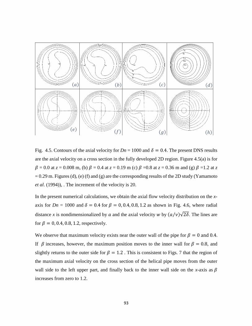
93

Fig. 4.5. Contours of the axial velocity for Dn = 1000 and 𝛿 = 0.4. The present DNS results

are the axial velocity on a cross section in the fully developed 2D region. Figure 4.5(a) is for

𝛽 = 0.0 at z = 0.008 m, (b) 𝛽 = 0.4 at z = 0.19 m (c) 𝛽 =0.8 at z = 0.36 m and (g) 𝛽 =1.2 at z

= 0.29 m. Figures (d), (e) (f) and (g) are the corresponding results of the 2D study (Yamamoto

et al. (1994)), . The increment of the velocity is 20.

In the present numerical calculations, we obtain the axial flow velocity distribution on the x-

axis for Dn = 1000 and 𝛿 = 0.4 for 𝛽 = 0, 0.4, 0.8, 1.2 as shown in Fig. 4.6, where radial

distance x is nondimensionalized by 𝑎 and the axial velocity 𝑤 by (𝑎 𝜈⁄ )√2𝛿. The lines are

for 𝛽 = 0, 0.4, 0.8, 1.2, respectively.

We observe that maximum velocity exists near the outer wall of the pipe for 𝛽 = 0 and 0.4.

If 𝛽 increases, however, the maximum position moves to the inner wall for 𝛽 = 0.8, and

slightly returns to the outer side for 𝛽 = 1.2 . This is consistent to Figs. 7 that the region of

the maximum axial velocity on the cross section of the helical pipe moves from the outer

wall side to the left upper part, and finally back to the inner wall side on the x-axis as 𝛽

increases from zero to 1.2.

(𝑎) (𝑏) (𝑐)

(𝑒)

(𝑑)

(𝑓) (ℎ) (𝑔)

94

Fig. 4.6. The distribution of the axial velocity for Dn = 1000 and 𝛿 = 0.4 on the center line

(y = 0).

4.2.5 Flux through the pipe

Figure 4.7 shows the flux ratio Q/Qs (where Q is the flux through the helical pipe and Qs is

the flux through the straight pipe) versus Dn with the same axial pressure gradient, obtained

by the present numerical calculation and by Yamamoto et al. (1994) for 𝛽 = 0.8 and 𝛿 =

0.4. As seen in Fig. 4.7, flux ratio decreases as Dn increases. Both results agree very well

with each other.

𝑤

(𝑎𝜈)√2𝛿

𝑥/𝑎

95

Fig. 4.7. Flux ratio Q/Qs for for Dn = 1000 and 𝛿 = 0.4.

4.3 Unsteady solutions

Yamamoto et al. (1998) performed the 2D linear stability analysis of the steady solutions

obtained by themselves for 𝛿 =0.1, and found that the critical Reynolds number remarkably

decreases as 𝛽 increases and becomes less than 400 if 𝛽 ≥ 1.2. This finding is very

surprising because the critical Reynolds number is very large (3331 by Canton et al.(2016))

for the toroidal pipe (𝛽 = 0) (Canton et al.(2016) and Piazza et al. (2011)) and the Hagen

Poiseuille flow (𝛽 = ∞) is linearly stable. However, their linear stability analysis was limited

to only the 2D analysis, so that the critical Reynolds number might be lower than what they

obtained although it gives the upper bound. In spite of that, the experimental study

(Yamamoto et al. (1995) and Hayamizu et al. (2008)) showed that the critical Reynolds

numbers obtained two-dimensionally are very close to those of the experimental study.

4.3.1 Method to obtain the critical Reynolds number

In order to obtain the critical Reynolds number, we repeated unsteady calculations changing

Re, where the initial condition is the steady solution obtained by the steady calculation. In

the present study, disturbances are expected to be naturally introduced as a numerical error

in the course of the simulation. If the unsteady solution converges to the steady solution, it is

regarded to be stable, while unstable if the unsteady solution keeps to fluctuate and does not

𝑄𝑄𝑠

⁄

𝐷𝑛

96

converge to the steady solution. By the above mentioned method, the critical Reynolds

number is determined as the value between stable and unstable Reynolds numbers. It should

be remarked that the criterion of stability and instability did not depend on the position of z

in the present study.

As an example, the results of time-evolution calculations are shown for 𝛽 = 0.6 and 𝛿 = 0.1.

The deviation of the time-evolution of the axial velocity on z-axis (𝑤𝑐) from the steady

solution (𝑤𝑐(𝑠)

) is shown at several positions of z on the center line. Time-evolution of the

axial velocity for Re = 1096 shows that its value quickly approaches zero as shown in Fig.

4.8(a). Therefore, the steady solution for Re ≤1096 is thought to be stable. Next, time-

evolution calculations were performed for Re ≥ 1100. It is seen in Fig. 4.8 (b) and (c) that

the value of the axial velocity does not approach zero but fluctuations for four values of z.

Therefore, the steady solutions for Re = 1100 is thought to be unstable and the critical

Reynolds number, 𝑅𝑒𝑐, lies between 1096 and 1100. We shall call the flow for 𝑅𝑒 > 𝑅𝑒𝑐

the super critical state. It is interesting that the magnitude of the deviation becomes larger

toward the downflow direction.

(a)

(f) t = 1.8s

𝑡 [𝑠]

𝑤𝑐−𝑤𝑐(𝑠) [𝑚/𝑠]

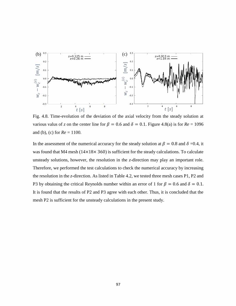
97

Fig. 4.8. Time-evolution of the deviation of the axial velocity from the steady solution at

various valus of z on the center line for 𝛽 = 0.6 and 𝛿 = 0.1. Figure 4.8(a) is for Re = 1096

and (b), (c) for Re = 1100.

In the assessment of the numerical accuracy for the steady solution at 𝛽 = 0.8 and 𝛿 =0.4, it

was found that M4 mesh (14×18× 360) is sufficient for the steady calculations. To calculate

unsteady solutions, however, the resolution in the z-direction may play an important role.

Therefore, we performed the test calculations to check the numerical accuracy by increasing

the resolution in the z-direction. As listed in Table 4.2, we tested three mesh cases P1, P2 and

P3 by obtaining the critical Reynolds number within an error of 1 for 𝛽 = 0.6 and 𝛿 = 0.1.

It is found that the results of P2 and P3 agree with each other. Thus, it is concluded that the

mesh P2 is sufficient for the unsteady calculations in the present study.

(b)

(f) t = 1.8s

(c)

(f) t = 1.8s


𝑡 [𝑠]


𝑡 [𝑠]

98

Table 4.2. Grid sensitivity analysis for unsteady calculations. The symbol ○ indicates the

stable and □ the unstable.

4.3.2 Critical Reynolds number for various 𝜷

We performed a comprehensive study of unsteady flow calculations over the range 0.6 ≤

𝛽 ≤ 1.8 for 𝛿 = 0.1. Figure 4.9 shows that the critical Reynolds number obtained by the

present DNS (shown with the symbol ●) decreases as 𝛽 increases, and that it becomes

minimum at 𝛽 = 1.6, then rapidly increases as 𝛽 further increases. It should be noted that

the 2D linear stability analysis by Yamamoto et al. (1998) (shown with the symbol ▽) gave

the minimum critical Reynolds number at 𝛽 = 1.4. We listed the values of the present

critical Reynolds number for various 𝛽 in Table 4.3.

As shown in Fig. 4.9, we may say that the stability characteristics obtained numerically by

DNS nearly agree with those of Yamamoto et al. (1998) for 𝛽 ≤ 1.4, but not for 𝛽 = 1.6. It

should be remarked that no linear stability result is available for 𝛽 = 1.8. The discrepancy

between the 2D linear stability analysis and the present DNS in the case for 𝛽 = 1.6 may

suggest that 3D disturbances dominate the marginal instability state. In Fig. 4.9, the

experimental results by Hayamizu et al. (2008) are also plotted with the symbol ○. Though

they nearly agree with the present results, no experimental data is available for 𝛽 = 1.6 and

1.8.

Mesh Mesh Size Re Instability of the

helical pipe

Total number of

grid M N L

P1 14 × 18 × 360 1093 ○

433440 1094 □

P2 14 × 18 × 540 1096 ○

650160 1097 □

P3 14 ×18 × 720 1096 ○

866880 1097 □

99

Fig. 4.9. The critical Reynolds number in the 𝑅𝑒-𝛽 plane for 𝛿 = 0.1. The symbol ● denotes

the present DNS results. The results of the 2D linear stability by Yamamoto et al. (1998) are

shown with the symbol ▽, and the experimental data by Hayamizu et al. (2008) with the

symbol ○.

Table 4.3. The critical Reynolds number. 𝑅𝑒𝑐1 is the Reynolds number of the marginally

stable state and 𝑅𝑒𝑐2 is that of the marginally unstable state.

𝛽 𝑅𝑒𝑐1 𝑅𝑒𝑐2 𝛽 𝑅𝑒𝑐1 𝑅𝑒𝑐2

0.6 1096 1097 1.55 124 125

0.8 716 717 1.6 105 106

1.0 479 480 1.65 143 144

1.2 317 318 1.7 219 220

1.4 227 228 1.8 553 554

1.5 168 169

4.3.3 Time-evolution of the equi-surface of the axial velocity for 𝜷 = 𝟎. 𝟔

𝑅𝑒 𝑐

100

In order to investigate the time-evolution of the disturbances of the supercritical state for the

low torsion case, we plot equi-sufaces of the axial velocity, w, in the middle region of the

helical pipe (0.43 m ≤ 𝑧 ≤ 0.90 m) for Re =1100, 𝛽 = 0.6 and 𝛿 =0.1 in Fig. 4.10, where

Re is slightly above the marginal instability (see Table 4.3). The figures show the time-

evolution of the constant value surface of w = 0.41 m s⁄ for 0.5 s ≤ 𝑡 ≤ 5 s. In Fig. 4.10(a),

the wall of the helical pipe is shown, where the flow goes from the bottom to the top. Figures

4.10 (b)-(e) show the initial evolution of the flow for 0.8 s ≤ 𝑡 ≤ 1.5 s. It is found that nearly

2D (uniform in the z-direction) flow evolution terminates at 𝑡 ≈ 0.8 s. After t =1 s, 3D

surface modification begins as shown in Figs. 4.10(d)-(e). For 𝑡 ≥ 1.8 s, nonlinear flow

evolution seems to begin as shown in Figs. 4.10(f)-(h). It is found that nonlinear behavior of

the flow seems to be stronger in the downstream region (in the upper part of the figures)

because the instability grows in the main flow direction.

(a) (b) (c) (d) (e) (f) (g) (h)

Fig. 4.10. Equi-surface of the constant velocity of w for Re = 1090, 𝛽 = 0.6 and 𝛿 =0.1 in

the region z = 0.43 m-0.90 m. Figure 7(a) is the pipe wall, (b) at t = 0.5 s, (c) t = 0.8 s, (d) t

= 1.0 s, (e) t = 1.5 s, (f) t = 1.8 s, (g) t = 3.0 s and (h) t = 5.0 s.

101

Figures. 4.11(a)-(h) shows that the flow fluctuates in the form of the two vortex solution. It

is found that in the initial time period, the vortex pattern nearly consists of two vortices in

the upper and lower hemispheres of the cross section. As time proceeds, the lower vortex

moves to the center of the cross section, and the upper vortex becomes smaller and weaker.

The maximum velocity region on the cross section does not move but stays in the second

quadrant of the cross section throughout the time visualized as shown in Fig. 4.12. It is

interesting that after t =5, the contour lines become complicated, which is very different from

those before the time t = 5. This is consistent to the non-periodic oscillation of the equi-Uz

surface presented in Fig. 12. Fig. 4.13 (a-d) shows that, in the initial time period, the vortex

nearly consists of two vortices at z = 0.774, which is the same as z = 0.39. However, for t >

7.2, we see that three-, four- and five- vortex patterns appear on the whole cross section. It

should be remarked that flow oscillation behavior of the secondary flow is similar in the time

interval 0.8 ≤ 𝑡 ≤ 1.2. It is found that the maximum axial velocity region stays in the left

upper corner of the cross section for 𝑡 ≤ 1.8. However, a new minimum region appears in

the right lower corner of the cross section for 𝑡 ≥ 2 as shown in Fig. 4.14. After t =5, the

contour line of the axial velocity becomes complicated as shown in Fig. 4.14(e-h), which is

quite different from the behavior for 𝑡 ≤ 5 shown in Fig. 4.10(a-d). It is to be noted that at z

= 0.774, the behavior of the axial velocity is consistent to the non-periodic oscillation of the

equi-Uz surface presented in Fig. 4.10. Finally, it is concluded that two-vortex pattern of the

secondary flow is kept throughout the time visualized at z = 0.39, while it is destroyed for t

> 7.22 at z = 0.774. This implies that a strong 3D instability occurs in some region between

z = 0.39 and z = 0.774.

102

Fig. 4.11. Vector plots of the secondary flow for Re =1090, and 𝛽 = 0.6 at z = 0.39, where

an outer wall is on the right-hand side of each figure.. Figure 4.11(a) is for 𝑡 = 0.2s, (b) 𝑡 =

1.2s, (c) 𝑡 = 1.8s, (d) 𝑡 = 2.1s, (e) 𝑡 = 5s, (f) 𝑡 = 7.2s, (g) 𝑡 = 8s, and (g) (c) 𝑡 = 9.35s .

Fig. 4.12. Contours of the axial flow for Re =1090, and 𝛽 = 0.6 at z = 0.39. 𝑊𝑚𝑎𝑥 is

maximum position of the axial velocity., where an outer wall is on the right-hand side of

each figure.. Figure 4.12(a) is for 𝑡 = 0.2s, (b) 𝑡 = 1.2s, (c) 𝑡 = 1.8s, (d) 𝑡 = 2.1s, (e) 𝑡 = 5s,

(f) 𝑡 = 7.2s, (g) 𝑡 = 8s, and (g) (c) 𝑡 = 9.35s .

g h

𝑏 𝑐 𝑑

𝑒 f

a

g h

𝑏 𝑐 𝑑

𝑒 f

a

𝑊𝑚𝑎𝑥

103

Fig. 4.13. Vector plots of the secondary flow for Re =1090, and 𝛽 = 0.6 at z = 0.774, where

an outer wall is on the right-hand side of each figure.. Figure 4.13(a) is for 𝑡 = 0.2s, (b) 𝑡 =

1.2s, (c) 𝑡 = 1.8s, (d) 𝑡 = 2.1s, (e) 𝑡 = 5s, (f) 𝑡 = 7.2s, (g) 𝑡 = 8s, and (g) (c) 𝑡 = 9.35s .

Fig. 4.14. Contours of the axial flow for Re =1090, and 𝛽 = 0.6 at z = 0.774. 𝑊𝑚𝑎𝑥 is

maximum and 𝑊𝑚𝑖𝑛 is minimum position of the axial velocity., where an outer wall is on the

right-hand side of each figure.. Figure 4.14(a) is for 𝑡 = 0.2s, (b) 𝑡 = 1.2s, (c) 𝑡 = 1.8s, (d) 𝑡

= 2.1s, (e) 𝑡 = 5s, (f) 𝑡 = 7.2s, (g) 𝑡 = 8s, and (g) (c) 𝑡 = 9.35s .

g h

𝑏 𝑐 𝑑

𝑒 f

a

g h

𝑏 𝑐 𝑑

𝑒 f

a

𝑊𝑚𝑎𝑥

104

4.3.4 Time-evolution of the equi-surface of the axial velocity for 𝛽 = 1.6

We plot equi-surface of w in the middle region of the helical pipe (0.44 m ≤ 𝑧 ≤ 0.66 m)

for Re = 110, 𝛽 = 1.6 and 𝛿 = 0.1 in Fig. 4.15, where Re is slightly above the marginal

instability (see Table 4.3). It should be remarked again that the critical Reynolds number

obtained by the present 3D DNS study is much lower than that obtained by the 2D linear

stability analysis (Yamamot0 et al. (1998)). The figures show the time-evolution of the

constant value surface w = 0.041m s⁄ , for 2 s ≤ 𝑡 ≤ 7.2 s. In Figs. 4.15(e)-(g), the

occurrence of explosive 3D instability is clearly seen after t = 6.8 s in the downstream region.

(a) (b) (c) (d) (e) (f) (g)

Fig. 4.15. Equi-surface of the constant velocity of w for Re = 110, 𝛽 = 1.6 and 𝛿 =0.1 in the

region z = 0.42 m-0.66 m. Figure 8(a) is the pipe wall, (b) at t = 2.0 s, (c) t = 5.0 s, (d) t =

6.6 s, (e) t = 6.8 s, (f) t = 7.0 s and (g) t = 7.2 s.

Since 3D disturbances is found to dominate the marginal instability state for 𝛽 = 1.6, we

visualize 3D vortical structures of the disturbance at the marginal state in Fig. 4.16, where

we plot the equi-Q value surface (see Lesieur et al. (2005)) at the same region of Fig. 8 for

Re = 110, 𝛽 = 1.6 and 𝛿 = 0.1. In Fig. 4.16, we clearly observe that the waveform appeared

for 𝑡 ≤ 5 and it broke down as time proceeds. Therefore, it is clear that the wave-form

105

disturbance is a trigger of the 3D instability of the helical pipe flow at very low Reynolds

numbers for 𝛽 = 1.6.

For the evolution of the disturbance, the wavenumber, k, plays an important role for for 𝑡 ≤

5. We obtained the wavenumber of the wave-form disturbance, k = 1.5, for 𝛽 = 1.6, where

the wavenumber is non-dimensionalized by a, the pipe radius. It is found that since the phase

speed of the wave-form disturbance is nearly zero, it is a standing wave. In a straight pipe,

however, it is well known that the low Reynolds number bifurcation occurs in the form of

travelling wave as obtained by Wedin and Kerswell (2004). Therefore, it is interesting to

study the relationship between the standing wave of the present calculation and the travelling

wave of a straight pipe flow.

(a) (b) (c) (d) (e) (f) (g)

Fig. 4.16. Equi-Q value surface for Re = 110, 𝛽 = 1.6 and 𝛿 =0.1 in the region z = 0.42 m-

0.66 m. Figure 9 (a) is the pipe wall, (b) at t = 2.0 s, (c) 5.0 s, (d) 6.6 s, (e) 6.8 s, (f) 7.0 s and

(g) 7.2 s.

4.4 Discussion and conclusion

In this study, we conducted 3D DNS of the viscous incompressible fluid flow through a

helical pipe with circular cross section. We obtained steady solutions for 𝛿 = 0.4 and

compared them with those by the 2D study (Yamamoto et al. (1994)). We obtained the

106

critical Reynolds numbers of the laminar to turbulent transition by unsteady calculations for

𝛿 = 0.1 and compared the results with the previous studies (Yamamoto et al. (1998) and

Hayamizu et al. (2008)), where 𝛽 was changed from 0.6 to 1.8.

In the steady calculations, we found the existence of the fully developed 2D flow region.

Comparison of the present results on the cross section of the pipe in the fully developed 2D

flow region with those by the 2D study (Yamamoto et al. (1994)) shows a very good

agreement. In the present steady calculations, we observe that the secondary flow with two

vortices exhibits a topological change into a single large vortex structure as 𝛽 increases.

By conducting 3D unsteady calculations, we obtained the critical Reynolds numbers which

give the critical states of the laminar to turbulent transition of the helical pipe flow. The

results nearly agree with the preceding experimental data (Hayamizu et al. (2008)) as well as

the 2D linear stability analysis Yamamoto et al. (1998) for 𝛽 ≤ 1.4. However, for 𝛽 ≥ 1.5,

the critical Reynolds numbers obtained in the present study are much lower than those in the

former studies.

It is found that an explosive 3D evolution of the disturbance occurs in the marginal instability

state for 𝛽 = 1.6, and the disturbance breaks down into turbulence in the downstream region

as time proceeds. It is interesting that we found a vortical structure of the standing-wave

disturbance and it is destroyed in the downstream region as time proceeds, which indicates

that the standing-wave disturbance is a trigger of 3D instability at low Reynolds numbers.

For 𝛽 ≤ 1.4, on the other hand, nearly 2D disturbances grow in the initial period, then

become 3D gradually.

It is very interesting that visualization of the time evolution of disturbances shows the change

as follows: nearly two-dimensional state → global three-dimensional modification → highly

nonlinear behaviours → stationary nonperiodic oscialtion. We also found that the flow

oscillates between asymmetric two-, three-, four- and five- vortex solutions in the stationary

nonperiodic oscillation. In that period, the region of the maximum axial velocity occurs at

the left upper corner and the minimum at the right lower corner of the cross section.

107

Chapter 5

Effect of Torsion on the Friction Factor of Helical Pipe Flow


In this study, a comprehensive numerical study will be presented by 3D direct numerical

simulations of a viscous incompressible fluid flow through a helical pipe with a circular cross

section. The curvature,𝛿, torsion parameter, 𝛽, and the Reynolds number will be taken as

various. The main objective of this study is to numerically investigate the influence of torsion,

𝛽, on the friction factor in laminar helical pipe based on the comparison with the experimental

results of several helical circular pipes having different pitches and non-dimensional

curvature. Friction factor of the fully developed region is important in many branches of

engineer to determine the pumping power needed to overcome torsion- curvature induced

pressure losses. The asymptotic behavior of the friction factor of helical pipe flow may be

helpful to discuss a good physical insight and for engineering application. Finally, analysis

of existing region of the global peak of the friction factor within the range of torsion

parameter may give the advance study in engineering applications


Develop a new model and method to investigate the 3D flow characteristics and

friction factor through a helical pipe.

Find the friction factor of the helical pipe flow compared with the experimental data.

Expect a general scenario of the friction factor when the torsion parameter, curvature

and the Reynolds number are changed.

To clarify the effect of torsion on the friction factor of helical pipe flow.

Play a pioneer role in the range of torsion parameter where the torsion has no

remarkable effect on the friction factor of helical pipe flow over a wide range of the

Reynolds number.

Find a close relationship between the friction factor of curved pipe, helical pipe and

straight pipe.

108

Find the existing region of the global peak of the friction factor due to the effect of

torsion for all the Reynolds numbers and curvatures.

Help to understand the physics and mechanism of the friction factor behavior inside

a helical pipe, which manifests the importance in engineering applications.

5.2 Results

In this section, the results of the 3D DNSs are presented. The friction factor obtained by

DNSs are compared with those of an experimental study (Yamamoto et al. (1995)) of the

helical pipe for a wide range of 𝛽. We examined two types of helical pipe with different

curvature, for each of which we considered seven values of torsion (case I-VII), to compare

the numerical results with the experimental data (Yamamoto et al. (1995)) . The curvature

was around 0.1 for Type-1 and 0.05 for Type-2. The geometric parameters of the helical pipes

are listed in Table 5.1.

Table 5.1: Characteristic lengths of the helical pipes

Type-1

Case β τ R[mm] h [mm] 2a [mm] δ

I 0.45 0.203 15.0 30.00 15.26 0.1017

II 0.74 0.327 5.00 16.58 11.84 0.0987

III 0.91 0.398 2.50 10.31 8.68 0.0964

IV 1.11 0.501 3.00 14.70 15.35 0.1023

V 1.17 0.510 1.50 8.08 8.53 0.0947

VI 1.57 0.708 1.50 10.50 15.18 0.1012

VII 1.70 0.756 1.00 7.68 11.81 0.0984

Type-2

Case β τ R[mm] h [mm] 2a [mm] δ

I 0.48 0.154 15.0 45.00 15.38 0.0513

II 0.76 0.238 5.00 23.98 11.93 0.0497

III 0.92 0.289 2.50 14.79 8.79 0.0488

IV 1.11 0.354 3.00 21.00 15.16 0.0505

V 1.18 0.364 1.50 11.52 8.54 0.0475

VI 1.60 0.512 1.50 14.93 15.43 0.0514

VII 1.71 0.537 1.00 10.91 11.81 0.0492

109

The computational mesh numbers were varied in order to check the numerical accuracy. We

obtained the steady solutions at Re = 200 and 𝛿 = 0.1 for 𝛽 = 1.2 for five types of mesh,

which are named M1, M2, M3, M4, and M5 as listed in Table 5.2. For each mesh, the

volumetric flux through the pipe, 𝑄, the maximum axial velocity, 𝑤𝑚𝑎𝑥 , and the total

number of grids are shown in Table 5.2. From Table 5.2, we concluded that M4 is appropriate

for the computation in the present study.

Table 5.2. Grid sensitivity analysis for Re = 200 and 𝛿 = 0.1 at 𝛽 = 1.2

In the confusing scenario of orthogonal and non-orthogonal helical coordinates, Germano

(1982) found an advantage of the orthogonal system of helical coordinates that it can be easily

generalized to a generic system of coordinates in the normal plane. On the basis of the

orthogonal helical coordinate system, Yamamoto et al. (1994) numerically investigated

helical pipe flow using the spectral method assuming that the flow field is uniform in the

axial direction of the helical pipe.

In the present study, an appropriate mesh system with 3D orthogonal helical coordinates was

successfully created to conduct accurate DNSs of helical pipe flow using an FVM-based

open-source computational fluid dynamics package (OpenFOAM). To evaluate numerical

accuracy, we compared the contour plot of the axial flow in the fully developed flow region

obtained by the present 3D DNS with that obtained in the spectral study of Yamamoto et al.

(1994), as shown in Fig. 5.1. By observing the maximum axial velocity and the shape of the

contour pattern in Fig. 5.1, we found good agreement between the present DNS and the

spectral result. The contour lines are drawn at increments of 20 in the axial velocity from the

Mesh

name

Mesh size Q

[m3 s⁄ ]

𝑤𝑚𝑎𝑥


grids M N L

M1 8 × 11 × 360 1.1908× 10−4 83.68 149760

M2 10 ×13 × 360 1.1907× 10−4 85.41 223200

M3 12 ×16 × 360 1.2039× 10−4 86.56 328300

M4 14 ×18 × 360 1.2042× 10−4 88.23 433440

M5 16 ×21 × 360 1.2041× 10−4 88.19 576000

110

pipe wall for both the present results and the spectral study, where the axial velocity is

nondimensionalized by dividing by (𝑎 𝜈⁄ )√2𝛿.

(a) (b)

Fig. 5.1. Contours of the axial velocity for Re = 145 and 𝛿 = 0.4. The present DNS results

are the axial velocity on a cross section in the fully developed region. (a) 𝛽 =0.8 at z = 0.36

m. (b) corresponding results of the spectral study Yamamoto et al. (1994). The increment of

the contours is 20 and the outer wall is on the right side.

5.2.1 Comparison with experimental data for Type-1

A helical pipe becomes a toroidal pipe for 𝛽 = 0 and tends to a straight pipe as 𝛽 → ∞. The

secondary flow caused by the centrifugal force due to curvature is affected by torsion, which

results in different flow patterns from those in a toroidal pipe. It is interesting to note that

when 𝛽 is very small, a symmetric vortex pair of secondary flows similar to that is observed

in a toroidal pipe,6,11) and when 𝛽 increases, the secondary flow pattern changes into that of

one large vortex.

In order to compare the numerical results with the experimental data (Yamamoto et al.

(1995)), we conducted numerical calculations for 𝛽 = 0.45, 0.91, 1.17, 1.57, and 1.70 without

the turbulence model. Here, we used 𝛿 = 0.1 in the numerical calculations because the

experimental curvature is very close to 0.1 as listed in Table 5.1. In the present DNS

calculation, the friction factor of the pipe, f, is defined by

𝑓 = ∆𝑝

𝐿

2𝑎

𝜌𝑤2 , (5.1)

111

where ∆𝑝 is the pressure difference between two positions of the pipe in the region where the

flow is well developed and axially invariant, and the distance between the two positions is L.

We also compared the present DNS results with Eq. (5.2) (1959).

𝑓𝐼 = 1376√𝛿

(1.56+log10𝑅𝑒√𝛿)5.73 (5.2)

Note that Eq. (5.2) is valid for β = 0 or β << 1. For comparison, we plot the present DNS

results (○), the experimental data of Yamamoto et al. (1995) (□), and Eq. (5.2) (dotted line)

in Fig. 3. Equation (5.3) (dash-dotted line) represents 𝑓𝑠, the friction factor for a laminar flow

in a straight pipe.

𝑓𝑠 = 64

𝑅𝑒 (6)

Fig. 5.2. Friction factor of the helical pipe for β = 0.45 and 𝛿 = 0.1.

It was found that the DNS results are very close to the experimental data and reasonably close

to Eq. (5.2) over a wide range of the Reynolds number, 300 ≤ 𝑅𝑒 ≤ 3000 . Note that

Hayamizu et al. (2008) experimentally found the critical Reynolds number of the laminar to

turbulent transition to be 𝑅𝑒𝑐 = 2200 for β = 0.45 and 𝛿 = 0.1 by observing the unsteady

behavior of the secondary and axial flows. We found that the friction factor obtained by DNS

is in good agreement with the experimental data for 𝑅𝑒 ≤ 1500 ; for 𝑅𝑒 ≥ 1500 , the

112

agreement is only reasonably good, probably due to the turbulence effect. It was found that

the friction factor of the helical pipe is larger than that of a toroidal pipe for small β. In Fig.

5.2, it can be seen that the results of both the DNS and the experiment lie above the curve of

Eq. (5.2). It is well known that the friction factor of a straight pipe is smaller than that of a

toroidal pipe; thus, the friction factor curve for a straight pipe lies below than that of Eq. (5.2),

as shown by Eq. (5.3) in Fig. 5.2.

Fig. 5.3. Friction factor of the helical pipe flow at 𝛿 = 0.1 for β = 0.91.

The friction factor of the helical pipe obtained by the present DNS without turbulence models,

which is very close to the experimental data, decreases as β increases and is in fairly good

agreement with that of a toroidal pipe (Eq. (5.2)) for β = 0.91 as shown in Fig. 5.3.

Re

f

113


In Fig. 5.4, we find that the DNS results of the friction factor are in good agreement with the

experimental data. It is interesting that the friction factor decreases with increasing Re, and

appears below the curve for a toroidal pipe given by Eq. (5.2) but above the curve of Eq.

(5.3) for β = 1.17.


Re

f

Re

f

114


Figures 5.5 and 5.6 show the friction factor of the helical pipe for β = 1.57 and 1.70,

respectively, where the present DNS results are close to the experimental data. It was found

that the friction factor decreases as β increases further. The friction factor approaches that of

a straight pipe for low Reynolds numbers.

Finally, from Figs. 5.1-5.6, we observed that the friction factor of the helical pipe is greater

than that of a toroidal pipe for small β, and the friction factor gradually decreases and

approaches that for a straight pipe as β increases to over 1.0. Therefore, the effect of torsion

on the friction factor of the helical pipe becomes marked if β exceeds about 1.0, which is in

good agreement with the experimental results (Yamamoto et al. (1995)).

5.3 Axial flow distribution for Type-1

In this subsection, we study the axial flow distribution in the well-developed axially invariant

region. On the cross section, a high axial flow velocity yields a centrifugal force toward the

outside, so that a fluid particle with a high axial velocity subjected to a large centrifugal force

is moved to the outer region.

Re

f

115

In the present DNS, we obtain the axial velocity distribution along the x-axis for 𝑅𝑒 = 1000

and 𝛿 = 0.1 over a wide range of 𝛽 as shown in Fig. 5.7, where x is nondimensionalized by

dividing 𝑎 and the axial velocity 𝑤 is nondimensionalized by dividing by 𝑤.

In. Fig. 5.7, we find that a position with the maximum velocity exists near the outer wall of

the pipe for 𝛽 = 0.45. If 𝛽 increases, however, the position of the maximum axial velocity

moves to the inner side and lies near the inner wall for 𝛽 = 0.91. When 𝛽 becomes still larger,

the position of the maximum axial velocity returns to the center of the cross section and the

axial velocity distribution approaches that of the Hagen-Poiseuille flow.

In Fig. 5.7, we see that the maximum axial velocity gradually increases for 𝛽 ≤ 1.17 as 𝛽

increases, and it becomes maximum for 𝛽 ≅ 1.17. For 𝛽 > 1.17 , the maximum axial

velocity decreases gradually. Note that on the cross section, the pressure curve slowly

increases from the inner to outer wall along the x-axis and the maximum pressure lies on the

outer wall as shown in Fig. 5.8. Here, the pressure, p, is nondimensionalized by dividing by

(𝑎 𝜈)⁄ 2 1

𝜌 .

Fig. 5.7. Distribution of the axial velocity for 0.45 ≤ 𝛽 ≤ 1.70 and Re = 1000 at 𝛿 = 0.1

on the center line (y = 0).

x/a

116

Fig. 5.8. Distribution of pressure for 0.45 ≤ 𝛽 ≤ 1.70 and Re = 1000 at 𝛿 = 0.1 on the

center line (y = 0).

5.4 Friction factor over a wide range of 𝜷

The characteristics of the friction factor of the helical pipe have been described so far. In

order to show them comprehensively, we plot the values of the friction factor obtained from

the present DNS over the wide range of 0.02 ≤ 𝛽 ≤ 2.8 for three Reynolds numbers (Re =

80, 300, and 1000). Figures 5.9-5.11 and Figs. 5.12-5.14 show the friction factor of the helical

pipe for 𝛿 = 0.1 and 0.05, respectively.

In Fig. 5.9-5.14, the friction factor of the helical pipe experimentally obtained by Yamamoto

et al. (1995)) is plotted as squares (■) and that obtained by the present DNS is plotted as

circle (●). Equations (5) and (6) are also plotted in the figures. Note that no experimental data

exists for Re = 80 in Figs. 5.9 and 5.12.

5.4.1 Friction factor for Type-1 (𝜹 = 𝟎. 𝟏)

x/a

117

Fig. 5.9. Friction factor of the helical pipe for Re = 80 at 𝛿 = 0.1.

In Figs. 5.9-5.11, it is shown that the friction factor first increases from that of a toroidal pipe

and then almost monotonically decreases to that of a straight pipe as 𝛽 increases from zero.

The maximum of the friction factor occurs at 𝛽 ≅ 0.3 for Re = 80 and 300 and at 𝛽 ≅ 0.2

for Re = 1000. The present DNS results agree reasonably well with the experimental data

for Re = 300 and 1000, which supports the accuracy of the present calculations.


f

f

118

Although the results of Liu and Masliyah (1993) for Dn = 300 and 𝛿 = 0.16 (Fig. 19(a) in

their paper), which correspond to 𝑅𝑒 ≅ 250 since 𝐷𝑛 = 𝑅𝑒√𝛿, qualitatively agree with the

present results for Re =300, the relative increase in the peak value from that for a toroidal

pipe is slightly different. We found that the relative increase in the present DNS is 7% larger

than that of Liu and Masliyah (1993), and regarding the approach to the value for a straight

pipe, the present value approaches much more slowly than that observed by Liu and Masliyah

(1993). It is noteworthy that for a low Reynolds number (Re = 80), the friction factor has no

peak in the result of Liu and Masliyah (1993) (Fig. 19(b) in their paper), where their value of

Dn =20 corresponds to Re =80 and 𝛿 = 0.0625. Because the present DNS results show good

agreement with the experimental data and the present DNS is 3D (two-dimensional (2D) in

Liu and Masliyah (1993)), it is very plausible that our results are more accurate than those of

Liu and Masliyah (1993).


In Fig. 5.11, we found that the friction factor rapidly decreases from the maximum value and

slowly tends to that of a straight pipe as 𝛽 increases for Re =1000. Note that in the region

0.8 ≤ 𝛽 ≤ 1.8 , Hayamizu et al. (2008) found that the steady solution is linearly unstable and

that unsteady solutions are expected to appear. Although, we did not calculate the time

average of the friction factor for unsteady solutions in the unstable region of Fig. 5.11, it is

interesting that the results of the present steady calculations are in good agreement with the

experiment data.

f

119

5.4.2 Friction factor for Type-2 (𝜹 = 𝟎. 𝟎𝟓)


It is shown in Figs. 5.12-5.14 that the friction factor first increases then decreases as 𝛽

increases. The friction factor monotonically decreases toward that of a straight pipe as 𝛽

further increases. The maximum of the friction factor occurs at 𝛽 ≅ 0.3 for Re = 80 and 300,

as respectively shown in Figs. 5.12 and 5.13, and at 𝛽 ≅ 0.2 for Re =1000 as shown in Fig.

5.14. For the Reynolds numbers Re =300 and 1000, the value of 𝛽 giving the maximum

friction factor is the same at 𝛿 = 0.1 and 0.05.

Although we have no experimental data available for the small Reynolds number of Re =80,

the experimental data for Re =300 and 1000 are in good agreement with the DNS results as

shown in Figs. 5.13 and 5.14. The present DNS results of the friction factor for Re =300 and

1000 at 𝛿 = 0.05 are qualitatively similar to the results at 𝛿 = 0.1, but the values of the

maximum the friction factor are smaller than those for 𝛿 = 0.1.

120



From the discussion on Figs. 5.9 -5.14, we can conclude that the formula for the friction

factor of a toroidal pipe is not applicable to a helical pipe for 𝛽 ≥ 0.1 at 𝛿 = 0.1 as illustrated

by the cases studied in the present paper. We found that the friction factor of the helical pipe

approaches that of a straight pipe for 𝛽 > 2.5 at low Reynolds numbers (Figs. 5.9-5.10 and

5.12-5.13) of Re =80 and 300. For the higher Reynolds number (Figs. 5.11 and 5.14) of Re

= 1000, the peak of the friction factor is sharp and the approach the value for a straight pipe

is slower than that at low Reynolds numbers. We list the calculated values of the friction

factor in Table 5.3.

f f

121

Table 5.3: Friction factors for three Reynolds numbers at 𝛿 = 0.1 and 0.05.

𝛿 = 0.1 𝛿 = 0.05

Case f Case f

𝛽 Re =80 Re = 300 Re = 1000 𝛽 Re = 80 Re = 300 Re = 1000

0.02 0.855023 0.316098

0.160373 0.02 0.828002 0.288205 0.135716

0.1 0.879217 0.343315 0.205309

0.1 0.845671 0.321137 0.169997

0.2 0.889863 0.363433 0.221278

0.2 0.854284 0.339921 0.184821

0.3 0.893296 0.375112 0.204154

0.3 0.852379 0.348112 0.175538

0.45 0.889213 0.368951 0.160806

0.48 0.848215 0.329384 0.144926

0.6 0.880045 0.359121 0.150001

0.6 0.846299 0.315156 0.129231

0.74 0.875791 0.349575 0.148332

0.74 0.844001 0.298492 0.125773

0.91 0.865968 0.331143 0.137681

0.92 0.838005 0.286531 0.121474

1.0 0.857328 0.314151 0.131084

1.0 0.832425 0.272459 0.119494

1.11 0.854577 0.290768 0.126872

1.11 0.827025 0.257889 0.11625

1.17 0.844429 0.273529 0.122608

1.18 0.827358 0.250459 0.110837

1.3 0.835134 0.267219 0.119010

1.3 0.826123 0.245237 0.104619

1.4 0.834749 0.260123 0.116265

1.4 0.823737 0.242384 0.100113

1.57 0.825541 0.251055 0.108944

1.60 0.819731 0.236993 0.095283

1.70 0.813712 0.245279 0.102894

1.71 0.817634 0.235875 0.094712

1.9 0.810629 0.241623 0.100317

1.9 0.809522 0.231359 0.093813

2.2 0.806061 0.240062 0.096842

2.2 0.806522 0.225904 0.091279

2.8 0.803658 0.230966 0.086121

2.8 0.804825 0.222186 0.081712

122

5. 5. Discussions and conclusion

A numerical study involving 3D DNSs of the flows through helical pipes has been conducted

to obtain the friction factor over a wide range of the torsion parameter, 𝛽, for three Reynolds

numbers, and two curvatures, The obtained results were compared with experimental data

and also the results of a previous study. For small 𝛽, we found that the friction factor of the

helical pipe becomes larger than that of a toroidal pipe. When β further increases, the friction

factor tends to decrease from that of a toroidal pipe after taking a maximum and approaches

that of a straight pipe. Therefore, the effect of torsion on the friction factor of the helical pipe

becomes large when β exceeds about 1.0, which is in good agreement with the experimental

results. We also found that the magnitude of the axial velocity is smaller than that of a toroidal

pipe but larger than that of a straight pipe for 𝛽 ≥ 1.17, which is consistent with the effect

of torsion on the friction factor.

The results of the present DNSs were in reasonably good agreement with the experimental

data1) for Re =300 and 1000, while no experimental data was available for Re = 80. The

numerical results obtained by Liu and Masliyah (1993)were qualitatively similar to the

present results for Re = 300 and 1000, but the relative peak value of the friction factor was

larger and the approach to the asymptotic value for a straight pipe was slower in the present

results than in the work of Liu and Masliyah (1993). In addition, although their friction factor

curve2) had no peak for a low Reynolds number of Re = 80, ours had a peak at nearly the

same value of β as that for Re = 300 and 1000. Because the present DNS results were 3D and

supported by the experimental data, while the simulation by Liu and Masliyah (1993) was

2D, our results are thought to be superior to those of Liu and Masliyah (1993). It is

noteworthy that we found a global peak of the friction factor over a wide range of 𝛽 for low

to high Reynolds numbers, where the value of the peak decreases as the Reynolds number

increases and the curvature decreases. It is interesting that the peak existed in the range of

0.2 ≤ 𝛽 ≤ 0.3 for all values of the Reynolds number and curvature studied in the present

paper; thus, the torsion parameter was found to play an important role in the helical pipe flow.

It is also interesting that the friction factor formula for a toroidal pipe, was not applicable for

123

𝛽 ≥ 0.1 as illustrated by the cases studied in the present paper, and that the friction factor of

a helical pipe gradually approached that of a straight pipe for 𝛽 > 2.5.

124

Chapter 6

Thermal flow through a helical pipe with circular cross section

6.1 Objectives and scope of this chapter

The study of heat transfer in a helical pipe has been performed extensively, both

experimentally and numerically, because of a lot of engineering applications and scientific

interest. Due to higher heat transfer efficiency compared to straight pipe configuration, heat

transfer in a helical pipe is frequently used in power generation, nuclear industries,

refrigeration and air-conditioning systems, heat recovery systems, food and dairy processes

and other thermal processing plants. A main flow feature in a helical pipe is the presence of

the secondary flow motion generated by the combined effects of centrifugal force and pitch-

induced torsion. The secondary vortices promote fluid mixing and in turn enhance heat

transfer performance resulting in larger pressure drop in the flow passage.

In this study, Laminar forced convective heat transfer in a helical pipe with circular cross

section subjected to wall heating is presented numerically by 3D DNS comparing with the

experimental data. Numerical calculations will be carried out over the wide range of torsion

parameter, 𝛽 , Reynolds number, Re, for three types of the Prandtl number. The main

objective of this study is to numerically investigate the effect of torsion on the averaged

Nusselt number (averaged over the peripheral of the pipe cross section) at the well-developed

axially invariant flow region supported by the experimental data. In this study, we will

investigate the heat transfer flow characteristics such as secondary flow, fluid trajectory of

the fluid particle and temperature distribution due to the effect of torsion.


Develop a new model and method to investigate the 3D forced convective heat

transfer in a helical pipe.

A way to find the appearance of the well-developed axially invariant flow region.

Find the effect of the heated wall and non-heated wall on the well-developed axially

invariant flow region.

125

To find the stabilizing or destabilizing effect of torsion on the secondary flow in a

helical pipe.

Find the general scenario of the averaged Nusselt number due to the effect of torsion

and the Prandtl number over the wide range of Reynolds number and comparison

with the experimental data.

Expect a general scenario of the averaged Nusselt number due to the effect of the

Reynolds number while the torsion is changed

Find the secondary flow, fluid trajectory of the fluid particle and temperature

distribution on helical pipes over the wide range of torsion and the Reynolds number.

Play a pioneer role in finding the local Nusselt number over the circle at the well-

developed axially invariant flow region.

Find a close relationship between the local Nusselt number and the vortical structure

of the secondary flow with heated wall in helical pipe flow.

To find the existence of the global minimum and global maximum of the averaged

Nusselt number.

Help to understand the physics and mechanism of the flow behavior with heat transfer

inside a helical pipe.

6.2 Results

In this section, the results of DNS are presented. In the first part, steady solutions obtained

by DNS are compared with the experimental data (Shatat (2010)) in the fully developed

region of the helical pipe for 𝛽 = 0.0012 and 𝛿 = 0.018. In the second part, we obtained

the Nusselt number averaged over the pipe circumference in consideration of the effect of

torsion. The computational mesh numbers have been varied in order to check the numerical

accuracy, where the number of mesh in the radial direction is M, and N in the circumferential

direction. The uniform mesh was generated in the z-direction, where the number of mesh is

L. We obtained the steady solutions at Re = 1633 and 𝛿 = 0.018 for 𝛽 = 0.0012 and Pr =

8.5 for four types of the mesh, which are named as M1, M2, M3 and M4 as listed in Table

6.1. For each mesh, the maximum axial velocity, 𝑤𝑚𝑎𝑥, the averaged Nusselt number, 𝑁𝑢

over the circumference of the pipe wall at a fully developed region and the total number of

126

grids are shown in Table 6.1. Based on Table 6.1, we concluded that M3 is sufficient for the

computation of the force convective heat transfer in a helical pipe.

Table 6.1: Grid sensitivity analysis for Re = 1633 and 𝛿 = 0.018 at 𝛽 = 0.0012

6.2.1 Nusselt number

The Nusselt number, Nu, defined in Eq. (7), is used as an index of the heat transfer of forced

convection from the uniformly heated wall. It should be pointed out that since the experiment

was performed for Pr = 8.5, we compared the present DNS results with the experimental data

for this case. To validate the present DNS, we obtained Nu for two cases of Pr. They are

plotted with the symbol ● for Pr = 8.5 and ▲ for Pr = 7.5 as a function of the Reynolds

number in Fig. 4, where Manlapaz and Churchill’s (1981) correlation formula

𝑁𝑢 = [(48

11+

51 11⁄

[1+1342 𝑃𝑟 𝐷𝑛2⁄ ]2)3

+ 1.816 (𝐷𝑛

1+1.15 𝑃𝑟⁄)3 2⁄

]1 3⁄

(6.1)

is also shown with the solid line and the experimental data with the symbol ■. It should be

remarked that Eq. (6.1) is valid for negligible torsion as β << 1.

As shown in Fig. 6.1, the averaged Nusselt number increases as Re increases. It is found that

the present DNS results for Pr = 8.5 is very close to the experimental data, and Eq. (6.1) over

the wide range of the Reynolds number, 1000 ≤ 𝑅𝑒 ≤ 4100. It should be pointed out that

Yamamoto et al. (1995) experimentally found the critical Reynolds number of the laminar to

turbulent transition, 𝑅𝑒𝑐 = 2600, for β = 0.002 and 𝛿 = 0.01 with no thermal effect, by

observing the unsteady behavior of secondary and axial flow. Since the velocity flow field is

hardly affected by the temperature field in the case of forced convection, the critical Reynolds

number may be nearly the same for the present forced convection.

Mesh

name

Mesh size 𝑁𝑢 𝑤𝑚𝑎𝑥


grid M N L

M1 8 × 11 × 360 15.38938 1.66007 249600

M2 10 ×13 × 360 16.53598 1.67090 372000

M3 12 ×16 × 360 17.82339 1.68025 527400

M4 14 ×18 × 360 17.84031 1.68158 722400

127

For Pr = 8.5, we found that for higher Reynolds numbers (𝑅𝑒 > 2600), the Nusselt numbers

obtained by the present DNS are a little higher than the values obtained experimentally, while

the Nusselt numbers by DNS are in an excellent agreement with the experimental data for

𝑅𝑒 < 2600. The small differences for 𝑅𝑒 ≥ 2600 are probably due to the turbulence effect.

We also found that Nu slightly decreases as the Pr decreases, as shown in Fig. 6.1 for Pr =

7.5. For Pr = 7.5, Nu is in fairly good agreement with Eq. (6.1) although the curve of Eq.

(6.1) for Pr = 7.5 is not shown in Fig. 6.1.

Fig. 6.1. The Nusselt number for 𝛽 = 0.0012 and 𝛿 = 0.018 . The symbols ● and ▲

represents the present DNS results for Pr = 8.5 and 7.5, respectively, and the experimental

data by Shatat (2010) with the symbol ■ for Pr = 8.5.

6.3 Torsion effect on the Nusselt number

In order to study the effect of torsion on the Nusselt number over the range of Reynolds

number, 1000 ≤ 𝑅𝑒 ≤ 4100, we conducted numerical calculations for 𝛽 = 0.10, 0.30, 0.45

and 0.80 at 𝛿 = 0.018 and 𝑃𝑟 = 4.02 without turbulence model. It should be remarked that

no experimental data nor numerical result is available for higher torsion case to the author’s

knowledge of literature. Since the present DNS results agree with the experimental data pretty

well for 𝛽 = 0.0012 as shown in Fig. 6.1, the accuracy of the present calculations is assured.

𝑅𝑒

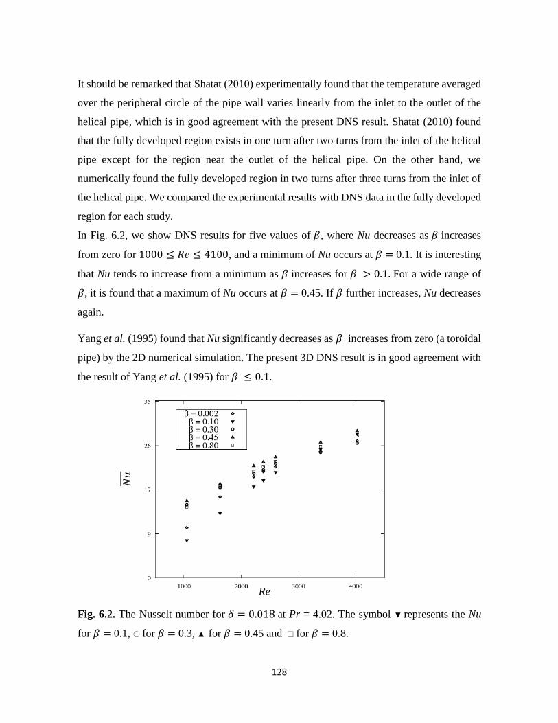
128

It should be remarked that Shatat (2010) experimentally found that the temperature averaged

over the peripheral circle of the pipe wall varies linearly from the inlet to the outlet of the

helical pipe, which is in good agreement with the present DNS result. Shatat (2010) found

that the fully developed region exists in one turn after two turns from the inlet of the helical

pipe except for the region near the outlet of the helical pipe. On the other hand, we

numerically found the fully developed region in two turns after three turns from the inlet of

the helical pipe. We compared the experimental results with DNS data in the fully developed

region for each study.

In Fig. 6.2, we show DNS results for five values of 𝛽, where Nu decreases as 𝛽 increases

from zero for 1000 ≤ 𝑅𝑒 ≤ 4100, and a minimum of Nu occurs at 𝛽 = 0.1. It is interesting

that Nu tends to increase from a minimum as 𝛽 increases for 𝛽 > 0.1. For a wide range of

𝛽, it is found that a maximum of Nu occurs at 𝛽 = 0.45. If 𝛽 further increases, Nu decreases

again.

Yang et al. (1995) found that Nu significantly decreases as 𝛽 increases from zero (a toroidal

pipe) by the 2D numerical simulation. The present 3D DNS result is in good agreement with

the result of Yang et al. (1995) for 𝛽 ≤ 0.1.

Fig. 6.2. The Nusselt number for 𝛿 = 0.018 at Pr = 4.02. The symbol ▼ represents the Nu

for 𝛽 = 0.1, ○ for 𝛽 = 0.3, ▲ for 𝛽 = 0.45 and □ for 𝛽 = 0.8.

Re

𝑁𝑢

129

The variation of Nu as a function of 𝛽 is shown in Fig.6.3 for three Reynolds numbers (Re =

1047, 1633 and 2600) at Pr = 4.02 and 𝛿 = 0.018. It should be be remarked that turbulence

may affect the value of Nu for Re > 2600 in experiments (Yamamoto et al. (1995). In Fig.

6.3, it is clear that Nu increases as Re increases. It is found in Fig. 6.3 that each curve of Nu

has two local minimums and two local maximums, where the global minimum exists at 𝛽 ≅

0.1 and the global maximum at 𝛽 ≅ 0.55 for any value of Re.

Fig. 6.3 The Nusselt number as a function of 𝛽 for 𝛿 = 0.018 at Pr = 4.02. The line of ○ for

𝑅𝑒 = 1047, □ for Re = 1633 and ▲ for 𝑅𝑒 = 2600.

6.4 Torsion effect on the secondary flow and temperature field

In the present 3D steady calculations, we found the fully developed flow region, where the

flow and temperature profiles do not change appreciably with the pressure gradient 𝜕𝑝 𝜕𝑧⁄

being nearly constant in the z-direction. This region lies in the part of the helical pipe after

three turns from the inlet of the helical pipe except for the region near the outlet. It should be

noted that forced convection in a helical pipe is affected by the secondary flow in the cross

section very much since the temperature field is strongly dependent on it. Therefore, it is

important to examine the secondary flow pattern in the forced convection.

𝛽

𝑁𝑢

130

A helical pipe is characterized by the value of 𝛽. When 𝛽 is zero, the helical pipe reduces to

a toroidal pipe, and if 𝛽 tends to infinity, it approaches a straight pipe. One of the important

differences between a laminar flow in a toroidal pipe and that in a helical pipe is that two

symmetrical vortices appear in the cross section for the toroidal pipe, while one dominates

another for the helical pipe due to the effect of the finite value of 𝛽.

In order to the study the cases of the minimal and maximal averaged Nusselt number, we

show the vector plots of the secondary flow for 𝛽 = 0.002 (small or negligible torsion case),

0.1 (minimal averaged Nusselt number), 0.55 (maximal averaged Nusselt number) at the fully

developed region for Re = 1047, 𝛿 = 0.018 and Pr =4.02 in Fig. 6.4. We also show the cut

section of the contours of the Q-value (the second invariant of the velocity gradient tensor)

surface (see Lesieur et al. (2005)) on the same figure.

For the small torsion case (𝛽 = 0.002), the axial flow yields the centrifugal force toward

outside of the pipe, and the fluid is moved from the inner to outer side. Because of mass

conservation, the fluid returns to the inner side around the upper and lower region of the cross

section. As a result, secondary flow is formed in the cross section exhibiting two symmetric

circulating cells shown in Fig. 6.4 (a). If torsion effect begins the work, the symmetric two-

cell pattern changes into the asymmetric two-cell pattern, as shown in Fig. 6.4 (b).

In Fig. 6.4 (b), we observe asymmetric secondary flow with a slightly weak anti-clockwise

vortex in the upper semicircle and a slightly strong clockwise vortex in the lower semicircle

for 𝛽 = 0.1. For 𝛽 = 0.55 in Fig. 6.4 (c), a large and strong vortex is produced in the lower

part of the cross section and the vortex becomes small and weak in the upper part. This shows

that, torsion of the pipe increases the strength of the vortex rotating in the same direction as

torsion. It should be noted that since torsion works as a rotational force, its effect is to induce

a circulating motion in the fluid. It is seen in Fig. 6.4 (c) that for 𝛽 = 0.55, the secondary

flow approximately consists of one large vortex, the center of which lies in the middle of

third and fourth quadrant of the cross section.

131

To supply additional insight into the vector plot of secondary flow, we show the 2D stream

lines, the projection of the trajectory of fluid particle on the cross section for several values

of 𝛽 as shown in Fig. 6.5, where the vortical structure is seen more clearly.

(a) (b) (c)

Fig. 6.4. Vector plots of the secondary flow and contours of the Q-value for Re = 1047, 𝛿 =

0.018 and Pr = 4.02, where an outer wall is on the right-hand side of each figure. The thick

lines denote the contour of the Q-value, where Q = 1.0 for all figures. Figure 6.4 (a) is for 𝛽

= 0.002 at z = 0.16 m, (b) 𝛽 = 0.1 at z = 5.95 m and (c) 𝛽 = 0.55 at z = 2.01 m.

(a) (b) (c)

Fig. 6.5. 2D stream lines of the secondary flow for Re = 1047, 𝛿 = 0.018 and Pr = 4.02,

where an outer wall is on the right-hand side of each figure. Figure 6.5 (a) is for 𝛽 = 0.002 at

z = 0.16, m (b) 𝛽 = 0.1 at z = 5.95 m and (c) 𝛽 = 0.55 at z = 2.01 m.

132

Then, we study the effect of torsion on the temperature field, where the temperature is non-

dimensionalized by T−𝑇𝑤

𝑇𝑤−𝑇𝑏. Figure 6.6 displays the temperature field in the cross section of

the helical pipe obtained by DNS at the fully developed flow region for 𝛽 = 0.002, 0.1 and

0.55 at Re = 1047, 𝛿 = 0.018 and Pr =4.02, where the wall of the helical pipe is

homogenously heated. The contour lines are drawn at every -10 of the temperature profile

for 𝛽 = 0.002 and 0.1 and every -20 of the temperature profile for 𝛽 =0.55.

It should be noted that the minimum temperature region exists inside the pipe because fluid

particles gain heat on the pipe wall and move into the inner pipe region convected by the

axial and secondary flow. It is found that a contour of the minimum temperature lies in the

middle of the first and second quadrant on the upper semi-circle for 𝛽 = 0.002 and the

second minimum lies in the middle of the third and fourth quadrant, as shown in Fig. 6.6 (a).

In Fig. 6.6 (b) for 𝛽 = 0.1, we notice that the temperature field becomes slightly asymmetric

similarly as the secondary flow in Fig. 6.4(b). As 𝛽 increases, the asymmetry of the

temperature field becomes conspicuous as shown in Fig. 6.6(c) for 𝛽 = 0.55. We find the

minimum temperature region lies in the second quadrant on the upper semi-circle of the cross

section.

(a) (b) (c)

Fig. 6.6. Contours of the temperature field for Re = 1047, 𝛿 = 0.018 and Pr = 4.02, where

the outer wall is on the right-hand side of each figure. Figure 6.6 (a) is for 𝛽 = 0.002 at z =

133

0.16 m, (b) 𝛽 = 0.1 at z = 5.95 m and (c) 𝛽 = 0.55 at z = 2.01 m. The increment of the

temperature is -10 for 𝛽 =0.002 and 0.1 and -20 for 𝛽 = 0.55.

6.5 Local Nusselt number

Figure 6.7 shows the distribution of the local Nusselt number along the peripheral circle over

the cross section at fully developed flow region for Re = 1047, 𝛿 = 0.018 and Pr = 4.02. The

torsion parameter, 𝛽, which controls the flow characteristics by the rotational force varies

from 0.002 to 0.55. The abscissa in Fig. 6.7 is the angle along the peripheral circle of the

cross section and ordinate the local Nusselt number at different positions on the circle.

Fig. 6.7. Local Nusselt number distribution for Re = 1047, 𝛿 = 0.018 and Pr = 4.02. The

solid is for 𝛽 = 0.002 at z = 0.16 m, a dashed line for 𝛽 = 0.1 at z = 5.95 m and a dotted line

for 𝛽 = 0.55 at z = 2.01 m.

For the small torsion case (𝛽 = 0.002), we found the wavy behavior of the local Nusselt

number on the circle as shown with a solid line in Fig. 6.7. This result is similar to the

previous study of Yang et al. (1995). In its wavy behavior, it is clearly seen that two maximal

134

peaks of the local Nusselt number exist in the upper and lower semicircles and the minimum

value of the local Nusselt number is located on the inside wall. We notice that the peak of the

local Nusselt number is slightly higher at the upper wall than at the lower wall. It is found

that the main contribution to the averaged Nusselt number comes from these two peaks.

It is interesting that for 𝛽 = 0.1, any peak of the local Nusselt number disappears and the

distribution of the local Nusselt number becomes rather flat as shown by a broken line in Fig.

10. The rotational force due to increase of torsion parameter weakened the two-cell pattern

of the secondary flow and consequently wiped out the peaks of the local Nusselt number. As

a result the averaged Nusselt number takes a bottom at 𝛽 ≅ 0.1.

However, if 𝛽 further increases and becomes 0.55, the distribution of the local Nusselt

number goes upward as shown by a dotted line in Fig. 6.7, so that the averaged Nusselt

number recovers its value and becomes greater than that for 𝛽 = 0.002. It is caused by a

strong swirling motion of the secondary flow at large torsion parameter. The moderate peak

of the local Nusselt number lies around the inside wall.

In summary, for small torsion parameter, heat transfer from the pipe wall to fluid occurs at

two local regions on the wall due to the two-cell pattern of the secondary flow. For large

torsion parameter, on the other hand, heat transfer occurs globally on the wall due to the large

one cell pattern of the secondary flow. For the intermediate torsion parameter, total heat

transfer becomes minimum because both the local and global heat transfer are not effective.


3D DNS study of the flow through helical pipes has been conducted and the averaged Nusselt

number was obtained for the wide range of torsion parameter, 𝛽, three Reynolds numbers,

Re = 1047, 1633 and 2600, three Prandtl numbers, Pr =8.5, 7 and 4.02 and curvature, 𝛿 =

0.018. Obtained results were compared with the experimental data (Shatat [1]) and also the

previous study (Yang et al. [3]).

135

In 3D steady calculations with homogeneously heated wall temperature, we found the

appearance of the fully developed flow region, where we compared the averaged Nusselt

number obtained by DNS with the experimental data and the formula by Manlapaz and

Churchill’s [12]. For low torsion parameter, 𝛽 = 0.0012, we found the Nusselt number of

the present DNS was in good agreement with the experimental data for Pr =8.5. If the Prandtl

number decreases, we found the Nusselt number slightly decreases at low torsion case, which

is in good agreement with the results by Yang et al. [3].

If 𝛽 increases from zero (a toroidal pipe), then we found the averaged Nusselt number of the

helical pipe begins to decrease than that of a toroidal pipe, and increases after taking the

global minimum at 𝛽 ≅ 0.1. If β further increases, we found a local maximum of the averaged

Nusselt number, which decreases and then takes the global maximum at 𝛽 ≅ 0.55 for any

value of the Reynolds number. For the wide range β, we found that the torsion effect is

remarkable on the averaged Nusselt number for any value of the Prandtl Number, and torsion

parameter was found to play an important role in the forced convection of helical pipe flow.

In order to obtain physical insight into the reason of variation of the averaged Nusselt number

as β changes, we plotted the secondary flow, 2D stream lines and the temperature field on

the cross section for several values of β. It was found that the secondary flow exhibits nearly

symmetric two-cell pattern for small β case, then becomes asymmetric and finally changes

into one-cell pattern as β increases. The temperature field changed from a slightly asymmetric

form to a strongly asymmetric form via an asymmetric form. We also plotted the local Nusselt

number over the peripheral circle and studied the topological change of the temperature field

as β increases. It was found that the minimum of the averaged Nusselt number occurred when

both the effect of the secondary flow with symmetric two-cell pattern and that with one-cell

pattern become feeble for 𝛽 ≅ 0.1. We hope the present result may contribute the

improvement of heat exchanger using helical pipes.

136

Chapter 7

Turbulent flow through a helical pipe with circular cross section


Fluid flows in a helical pipe has been attracting considerable attention because of abundant

applications not only to engineering but also to medical sciences. Flows in a helical pipe are

often in a turbulent state at high Reynolds numbers. Pressure gradient is needed to drive

turbulent flows in a pipe may be much larger than that for laminar flow in the presence of

turbulent eddy viscosity. Therefore, it is necessary to study turbulent helical pipe flow in

order to develop efficient transportation pipe system for liquids and gases. Due to the

combined effects of centrifugal force and pitch-induced torsion, the fluid flow in a helical

pipe differs from those in straight or toroidal (a helical pipe with a zero pitch) pipes. The

curved pipe inevitably has a finite pitch if it has several turns, and hence the pipe is more or

less in a helically coiled shape. The secondary flow caused by the centrifugal force due to

curvature is affected by torsion, which creates different flow patterns from those in a toroidal

pipe. The existence of complex secondary flows in the cross section is one of the remarkable

features of the fluid flow in a helical pipe.

In this study, a comprehensive numerical study will be presented for a viscous incompressible

turbulent fluid flow through a helical pipe with a circular cross section. Numerical

calculations are carried out for two helical circular pipes having different pitches and the

same non-dimensional curvature, 𝛿, with the wide range of the torsion parameter, 𝛽, and the

Reynolds number. The main objective of this study is to numerically estimate the critical

Reynolds number of transition turbulent to fully develop turbulent by observing the axial

flow distribution supported by the experimental data, and to find the best turbulence models

that can good predict the characteristics of turbulent flow behavior. In addition to that we

investigated the turbulent flow characteristics (such as the secondary flow, the axial flow and

the intensity of the turbulent kinetic energy) in a helical pipe by use of three turbulence

models incorporated in OpenFOAM comparing with the experimental data.

137


To investigate the turbulent flow characteristics through a helical pipe by different

turbulence models.

In 3D ensemble average steady calculations with several turns of a helical pipe, find

the appearance of the fully developed flow region.

Estimate the critical Reynolds number of the transition from transitional to fully

developed turbulent flow in a helical pipe by observing the axial flow distribution

based on the experimental data.

To clarify the consistency of the estimated critical Reynolds number in present study.

Find a general scenario of the behavior of the turbulent flow characteristics with the

ensemble-averaged secondary flow, the axial flow and the intensity of the turbulent

kinetic energy.

Find the best turbulence model that can predict the scenario of turbulent flow

characteristics.

To clarify, whether the momentum transfer due to turbulence dominates or not on the

secondary flow pattern of the turbulent helical pipe flow.

To conclude that the torsion effect is more remarkable on turbulent flows or laminar

flows by comparing the flow behavior of the turbulent and laminar flows,

Help to understand the physics and mechanism of the turbulent flow behavior inside

a helical pipe.

138

7.2. Results

Hayamizu et al. (2008) obtained the critical Reynolds numbers of laminar to turbulence

transition through a helical pipe with circular cross section in the Re- β plane. They also found

the trasitional and supercritical behaviors of disturbances over a wide range of torsion

paramter 0.02 ≤ 𝛽 ≤ 1.8. The critical Reynolds numbers are 1097, 717, 480, 318, 228, 106

and 554 for 𝛽 = 0.6, 0.8, 1.0, 1.2, 1.4, 1.6 and 1.8, respectively.

In this section, the results of the numerical simulations are presented. We first investigate the

transition to fully developed turbulence by comparing the experimental data with numerical

results. Then, we discuss the fully developed turbulent flow characteristics. We show the

results for the Reynolds number ranging from 3000 to 21000 with different pitches, where

the cases for torsion parameter β = 0.02 and 0.45 are addressed in section 7.1 and 7.2,

respectively. We confirmed that the flow attains a sufficiently developed equilibrium state in

the middle part of the helical pipe and the state continues up to near the outlet of the pipe

except for the region very close to the outlet.

Figure 7.1. A view of the 3.2 pitch helical pipe showing the three-pitch downstream cross

section for 𝛽 = 0.02 and 𝛿 = 0.1.

3 pitch

downstream

Cross section.

Inlet

Outlet

139

The computational mesh numbers have been varied in order to check the numerical accuracy.

In Fig. 7.2, we show the axial velocity distribution along the x-axis using RNG 𝑘 − 휀 model

at Re = 5320 for 𝛽 = 0.02 and 𝛿 = 0.1 for four types of the mesh, which are named as M1,

M2, M3 and M4 as listed in Table 7.1. For each mesh, the center line turbulent kinetic energy,

𝑘𝑐 = (𝑅𝑥𝑥 + 𝑅𝑦𝑦 + 𝑅𝑧𝑧) 2⁄ , the maximum axial velocity, 𝑤𝑚𝑎𝑥 , and the total number of

grids are listed in Table 6.1. Based on Table 7.1 and Fig. 7.2, we concluded that M3 is

sufficient for the computation of the turbulent helical pipe flow.

Table 7.1: Grid sensitivity analysis for Re = 5320 for 𝛽 = 0.02 at 𝛿 = 0.1.

Figure 7.2. Axial flow distribution on the x-axis for 𝛽 = 0.02 and 𝛿 = 0.1.

Mesh

name

Mesh size 𝑘𝑐

[𝑚2 𝑠2⁄ ]

𝑤𝑚𝑎𝑥


grid M N L

M1 8 × 11 × 360 8.0626× 10−3 1.3339 159744

M2 10 ×13 × 360 12.0239× 10−3 1.3479 238080

M3 12 ×16 × 360 15.5679× 10−3 1.3633 350208

M4 14 ×18 × 360 15.5317× 10−3 1.3653 462336

𝑤⟨ 𝑤⟩

⁄

𝑥/𝑎

140

7.3 Results of the case for β = 0.02

(A) Axial velocity distribution

In this subsection, we study the axial velocity distribution of the developing and fully

developed turbulence. The development of the boundary layer near the outer wall is more

delayed compared to that near the inner wall since the high axial flow region is moved to the

outer wall by the secondary flow. Hence the boundary layer thickness on the outer wall is

much smaller than that on the inner wall. In the present paper, we numerically obtained the

axial velocity distribution along the x-axis and y-axis on the cross section of three-pitch

downstream cross section (see Fig. 7.1) at 𝛽 = 0.02 and 𝛿 = 0.1 for the Reynolds number

ranging from 5000 to 21000, as shown in Fig. 7.3 and 7.4, respectively. Here, the radial and

vertical distance x and y is non-dimensionalized by 𝑎 and the axial velocity 𝑤 by ⟨𝑤⟩.

As shown in Fig. 7.3, it is clear that for low Reynolds numbers (Re = 5320 and 6880), any

turbulence model cannot predict well the axial velocity profile of the experimental results

especially in the inner region of the pipe (small 𝑥). It is interesting that for higher Reynolds

numbers (Re = 12140 and 20850), on the other hand, the axial velocity profile of the

experimental results is pretty well predicted by turbulence models although Launder-Sharma

𝑘 − 휀 model cannot predict well for Re = 20850 in the outer region (large 𝑥). The fact that

two turbulence models can predict the velocity profile of the experimental results for Re =

12140 and 20850 suggests that the flow attains the fully developed turbulent state in these

cases, and that the transition to fully developed turbulence occurs between Re = 12140 and

20850.

141

Fig. 7.3. Axial velocity distribution on the x-axis for 𝛽 = 0.02 at 𝛿 = 0.1. The outer wall is

on the right-hand side.

Figure 6.4 shows vertical cuts of the axial velocity at three-pitch downstream (see Fig. 7.1)

from the entrance for four Reynolds numbers. In Fig. 7.4, we observe that the axial velocity

profile has local maxima near the upper and lower wall, and that no turbulent model can

predict the axial velocity profile of the experimental data in low Reynolds numbers (Re =

5320 and 6880). For high Reynolds numbers (Re = 12140 and 20850), however, the

predictions of two turbulence models show a pretty good agreement with the experimental

data. For the largest Reynolds number (Re = 20850), the agreement is excellent. The reason

why Launder-Sharma 𝑘 − 휀 model cannot give a good prediction is due to the fact that it is

an isotropic turbulence model.

𝑤⟨ 𝑤⟩

⁄

𝑥/𝑎

(a) Re = 5320

𝑤⟨ 𝑤⟩

⁄

𝑥/𝑎

(b) Re = 6880

𝑤⟨ 𝑤⟩

⁄

𝑥/𝑎

(c) Re = 12140

𝑤⟨ 𝑤⟩

⁄

𝑥/𝑎

(d) Re = 20850

142

Fig. 7.4. Axial velocity distribution on the y-axis for 𝛽 = 0.02 at 𝛿 = 0.1. The upper wall is


(B) Secondary flow pattern on the cross section of the helical pipe

A helical pipe is characterized by finite torsion. When torsion is zero, the helical pipe reduces

to a toroidal pipe, and if torsion tends to infinity, it reduces to a straight pipe. One of the

important differences between a laminar flow in a toroidal pipe and that in a helical pipe is

there appear two symmetrical vortices in the cross section for the toroidal pipe, while these

vortices are not symmetrical for the helical pipe due to the effect of non-zero torsion.

Figure 7.5 shows the projection of the fluid velocity (secondary flow) on the cross section of

the helical pipe at the three-pitch downstream for 𝛽 = 0.02 and 𝛿 = 0.1 . Numerical

simulations were performed by use of Lien-cubic 𝑘 − 휀 and RNG 𝑘 − 휀 turbulence models.

(a) Re = 5320

𝑤⟨ 𝑤⟩

⁄

𝑦/𝑎

(b) Re = 6880

𝑤⟨ 𝑤⟩

⁄

𝑦/𝑎

(c) Re = 12140

𝑤⟨ 𝑤⟩

⁄

𝑦/𝑎

(d) Re = 20850

𝑤⟨ 𝑤⟩

⁄

𝑦/𝑎

143

Experimental results of the secondary flow for Re = 12140 were given by Wada (2010) and

those for Re = 20850 by Yamamoto et al. (2005). The reason why we consider the three-pitch

downstream cross section of the 3.2 pitch helical pipe both numerically and experimentally

is due to the fact that the experimental data were taken there.

Now, we investigate the patterns of the secondary flow for high Reynolds numbers (Re =

12140 and 20850) because turbulence models predict the experimental data fairly well for

high Reynolds numbers as discussed in section 7.1(A). In Fig. 7.5, it is found that the

ensemble-averaged (numerical simulation) or time-averaged (experiments) secondary flow

consists of uniform flow directed from the inner to outer sides of the helical pipe over almost

all the cross section both for Re = 12140 and 20850. The arrows in the figure show the

secondary velocity field. Recirculating regions associated with the back flow from the outer

to inner sides are very small both in the upper and lower semicircles. Flow structures are

similar for two turbulence models, Lien cubic 𝑘 − 휀 and RNG 𝑘 − 휀 turbulence models, and

experiments. It should be remarked that recirculating regions are hardly discerned in the

experimental data probably because the experimental resolution near the pipe wall is not

sufficient although some sign of the recirculating flow is seen in the upper and lower near

wall regions. It is interesting to note that two vortices associated with the recirculating flow

are clearly seen in the upper and lower hemisphere for 𝛽 = 0.02 if the flow is laminar (Re =

200) as shown in Fig. 7.6, which was numerically obtained by use of OpenFOAM without

any turbulence model. Therefore, the shrinking of these vortical regions may be due to the

turbulence effect of the enhancement of momentum transfer on the cross section.

Lien cubic 𝑘 − 휀 RNG 𝑘 − 휀 Experiment

(a) Re = 12140

x/a

144

Fig. 7.5. Vector plots of the secondary flow for β = 0.02 and 𝛿 = 0.1. Two figures on the

left-hand side are the results of numerical simulations and one on the right-hand side is the

experimental result. (a) is for Re = 12140 and (b) for Re = 20850. The outer wall is on the

right-hand side.

Fig. 7.6. Numerical result of vector plots of the secondary flow for β = 0.02 and 𝛿 = 0.1 at

Re = 200.

(C) Axial velocity pattern on the cross section

In this subsection, we study the axial velocity distribution on the cross section numerically

and experimentally for β = 0.02 and 𝛿 = 0.1 in Fig. 7.7(a-b). To compare with the

experimental results, we performed the numerical simulations with Lien-cubic 𝑘 − 휀 and

RNG 𝑘 − 휀 turbulence models. Experimental results of the axial flow for Re = 12140 were

(b) Re = 20850 x/a

y/a

145

given by Wada (2010) and those for Re = 20850 by Yamamoto et al. (2005). The contour

lines were drawn at every 0.2 of the axial velocity from the pipe wall, where the axial velocity

is non-dimensionalized by the mean axial velocity ⟨𝑤⟩.

In the contours of the axial velocity, we observe that the axial velocity is greatly influenced

by the outer flux of the secondary flow, since the maximum region of the axial velocity lies

in the outer side of the cross section. In general, the agreement between numerical and

experimental results is very good even if we observe the level of the contours. Especially, the

agreement of RNG 𝑘 − 휀 is noteworthy.

For 𝑅𝑒 = 12140 shown in Fig. 7.7(a), it is noticed that the contour of high axial velocity

region is shifted to the outer side of the cross section for both the results of the turbulence

model and the experimental data due to a large centrifugal force. The maximum value of the

non-dimensional axial velocity is 1.36 for Lien-cubic 𝑘 − 휀 model and 1.26 for RNG 𝑘 − 휀

model. It should be noted that the maximum axial velocity is 1.27 in the experiment, which

shows that RNG 𝑘 − 휀 model is in a excellent agreement with the experimental results. The

symbol ∗ represents the position of the maximum axial velocity.

For Re = 20850 shown in Fig. 7.7(b), a high axial velocity region moves further to the outer

wall direction. It is found that the maximum axial velocity is 1.29 for Lien-cubic 𝑘 − 휀 model

and 1.21 for RNG 𝑘 − 휀 model. The maximum axial velocity of the experiment is 1.21,

which shows again excellence of RNG 𝑘 − 휀 model. In the fully developed turbulent flow,

RNG 𝑘 − 휀 model is found to predict the axial velocity flow pattern very well with

comparison to the experimental results.

146

Fig. 7.7. Contours of the axial velocity for β = 0.02 and 𝛿 = 0.1. Two figures on the left-

hand side are the results of numerical simulations and one on the right-hand side is the

experimental result. (a) is for Re = 12140 and (b) for Re = 20850.

(D) Turbulent Intensity

The intensity of turbulence of a helical pipe obtained in the present numerical simulations is

shown in Fig. 7.8 for higher Reynolds numbers (Re = 12140 and 20850). Numerical

calculations were performed by Lien-cubic 𝑘 − 휀 model, RNG 𝑘 − 휀 model. We study the

turbulent intensity by view of the local peak level and contour patterns. Figure 6.8 shows the

contours of the non-dimensional turbulent intensity,(2𝑘)1 2⁄ /⟨𝑤⟩, at three pitch downstream

cross section from the inlet, where k is the intensity of the turbulent kinetic energy.

Experimental results of contours of the turbulent intensity were obtained by Yamamoto et al.

Lien cubic 𝑘 − 휀 RNG 𝑘 − 휀

(a) Re = 12140

Experiment

*

x/a

y/a

(b) Re = 20850

*

x/a

y/a

147

(2005). Figure 7.8(a) shows the contour of turbulent intensity for Re = 12140. It is found that

the peak of the turbulent intensity on the cross section lies near the outer wall by Lien-cubic

𝑘 − 휀 model and RNG 𝑘 − 휀 model, where the peak level is 0.22 for Lien-cubic 𝑘 − 휀 and

0.21 for RNG 𝑘 − 휀 model. It should be remarked that the experimental peak level is 0.19

near the outer wall. The agreement between numerical and experimental results is pretty good

as for the peak level. As for the shape of contours, we find that Lien-cubic 𝑘 − 휀 model agrees

with the experimental results pretty well but RNG 𝑘 − 휀 model does not predict well for Re

= 12140.

For a higher Reynolds number, Re = 20850, Fig. 7.8 (b) shows that the turbulent intensity is

relatively suppressed at the inner side and somewhat enhanced at the outer side of the helical

pipe. The peak level of the turbulent intensity is 0.18 for Lien-cubic 𝑘 − 휀 model and 0.17

for RNG 𝑘 − 휀 model. Since the experimental maximum value is 0.16, the agreement is also

good for this case. As for the shape of contours, Lien-cubic 𝑘 − 휀 model agrees pretty well

with the experimental results, although both turbulence models give nearly the same quality

of prediction.

Experiment Lien cubic 𝑘 − 휀

RNG 𝑘 − 휀

0.086 0.05 0.12 0.063 0.19

x/a

y/a

(a) Re = 12140

148

Fig. 7.8. Turbulent intensity, (2𝑘)1 2⁄ /⟨𝑤⟩ for β = 0.02 and 𝛿 = 0.1 at Re = 12140 and 20850,

where 𝑘 is the intensity of turbulent kinetic energy and ⟨𝑤⟩ the mean axial velocity. Two

figures on the left-hand side are the results of numerical simulations and one on the right-

hand side is the experimental result. (a) is for Re = 12140 and (b) for Re = 20850.

7.4 Results of the case for β = 0.45

(A) Axial velocity distribution

We first compared the numerical results of three RANS models with the experimental data

of the mean axial velocity profile for β = 0.45 and 𝛿 = 0.1, as shown in Figs. 7.9 and 6.10.

We considered the nine-pitch helical pipe for the comparison with the experimental results

of Yamamoto et al. (2005) and Hayamizu et al. (2008). We studied turbulence on the cross

section at the 8.3-pitch downstream of the helical pipe both numerically and experimentally.

Numerical and experimental results of the axial velocity profile is normalized by the ⟨𝑤⟩. We

plot the velocity profile for a low Reynolds number, Re = 3060, a middle Reynolds number,

Re = 5550, and high Reynolds numbers, Re = 9340 and 19910, along the radial x and vertical

y direction.

0.04 0.06

0.03 0.025

0.16

(b) Re = 20850

0.03

x/a

y/a

149

Fig. 7.9. Axial velocity distribution on the x-axis for 𝛽 = 0.45 at 𝛿 = 0.1. The outer wall is


In Fig. 7.9, it is clear that any turbulence model cannot predict well the experimental data for

the low Reynolds number case, Re = 3060, especially in the inner region of the helical pipe.

In the case of Re = 5550, RNG 𝑘 − 휀 model and Lien-cubic 𝑘 − 휀 model can predict the

experimental data in the positive and negative x region, respectively. It is remarkable that the

prediction of the axial velocity profile by RNG 𝑘 − 휀 model is excellent for Re = 9340 and

19910. It should be remarked that for low torsion parameter (β = 0.02), the flow attains the

fully developed states around Re = 12140, and that, for high torsion parameter (β = 0.45), the

flow seems to attain the fully developed state between Re = 5550 and 9340, which may be

slightly larger than 5550. Therefore, the torsion effect decreases the critical Reynolds number

of the transition to fully developed turbulence as it decreases the critical Reynolds number of

laminar to turbulent transition (Yamamoto et al. (1998)).

𝑤⟨ 𝑤⟩

⁄

𝑥/𝑎

(a) Re = 3060

𝑤⟨ 𝑤⟩

⁄

𝑥/𝑎

(b) Re = 5550

𝑤⟨ 𝑤⟩

⁄

𝑥/𝑎

(c) Re = 9340

𝑤⟨ 𝑤⟩

⁄

𝑥/𝑎

(d) Re = 19910

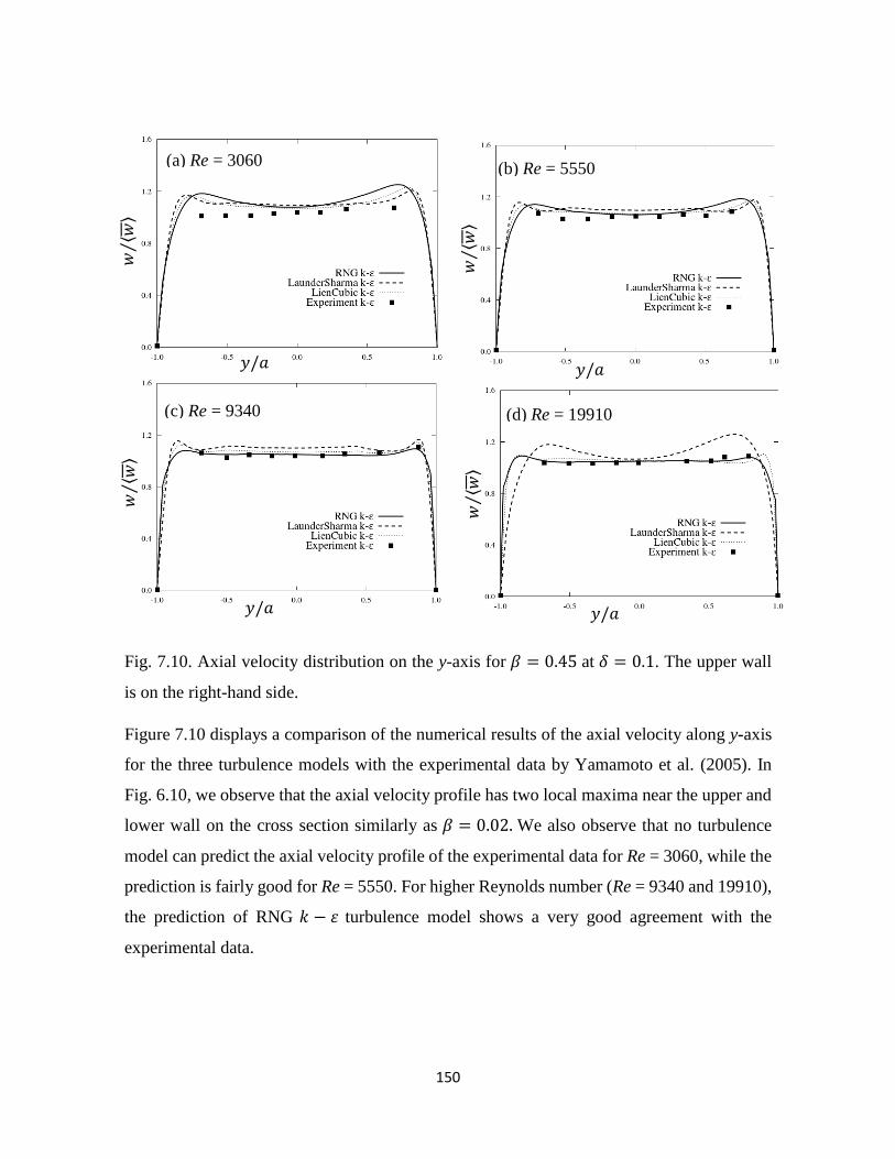
150

Fig. 7.10. Axial velocity distribution on the y-axis for 𝛽 = 0.45 at 𝛿 = 0.1. The upper wall

is on the right-hand side.

Figure 7.10 displays a comparison of the numerical results of the axial velocity along y-axis

for the three turbulence models with the experimental data by Yamamoto et al. (2005). In

Fig. 6.10, we observe that the axial velocity profile has two local maxima near the upper and

lower wall on the cross section similarly as 𝛽 = 0.02. We also observe that no turbulence

model can predict the axial velocity profile of the experimental data for Re = 3060, while the

prediction is fairly good for Re = 5550. For higher Reynolds number (Re = 9340 and 19910),

the prediction of RNG 𝑘 − 휀 turbulence model shows a very good agreement with the

experimental data.

𝑤⟨ 𝑤⟩

⁄

𝑦/𝑎

(a) Re = 3060

𝑤⟨ 𝑤⟩

⁄

𝑦/𝑎

(b) Re = 5550

𝑤⟨ 𝑤⟩

⁄

𝑦/𝑎

(c) Re = 9340

𝑤⟨ 𝑤⟩

⁄

𝑦/𝑎

(d) Re = 19910

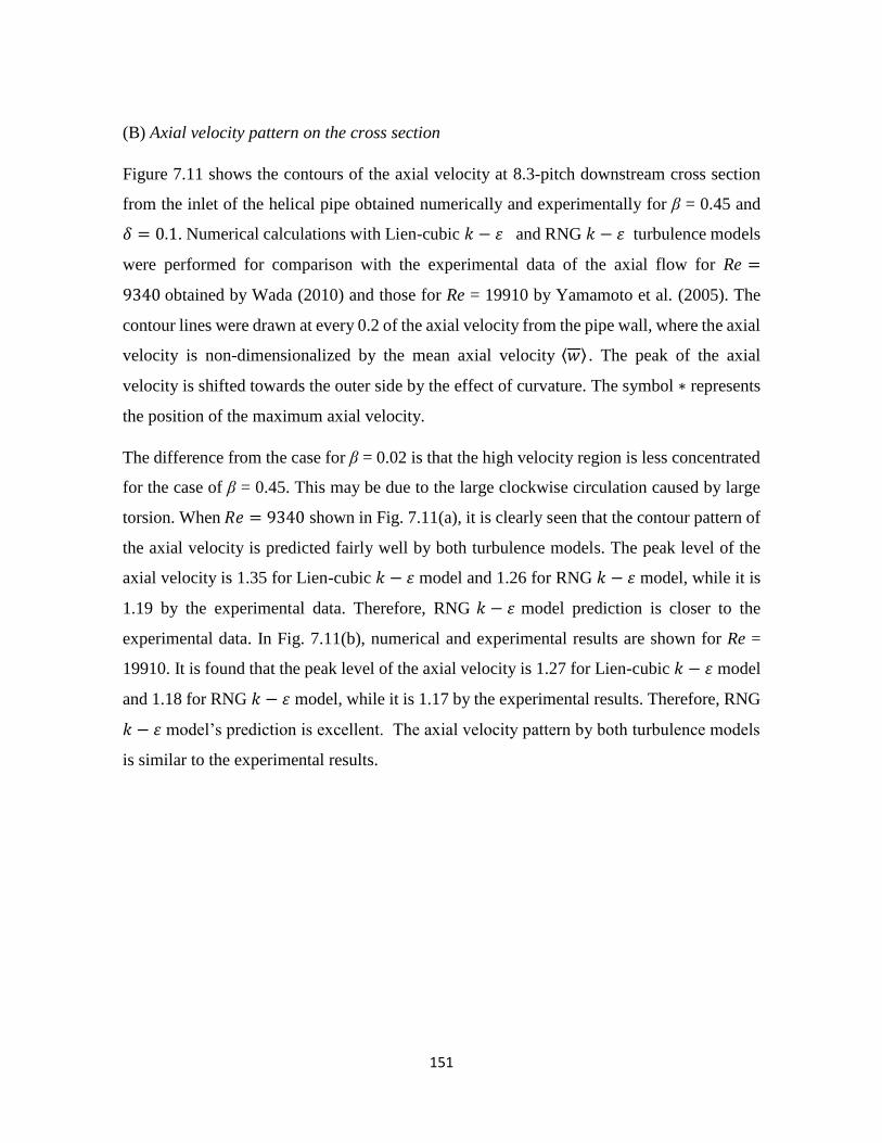
151

(B) Axial velocity pattern on the cross section

Figure 7.11 shows the contours of the axial velocity at 8.3-pitch downstream cross section

from the inlet of the helical pipe obtained numerically and experimentally for β = 0.45 and

𝛿 = 0.1. Numerical calculations with Lien-cubic 𝑘 − 휀 and RNG 𝑘 − 휀 turbulence models

were performed for comparison with the experimental data of the axial flow for Re =

9340 obtained by Wada (2010) and those for Re = 19910 by Yamamoto et al. (2005). The

contour lines were drawn at every 0.2 of the axial velocity from the pipe wall, where the axial

velocity is non-dimensionalized by the mean axial velocity ⟨𝑤⟩ . The peak of the axial

velocity is shifted towards the outer side by the effect of curvature. The symbol ∗ represents

the position of the maximum axial velocity.

The difference from the case for β = 0.02 is that the high velocity region is less concentrated

for the case of β = 0.45. This may be due to the large clockwise circulation caused by large

torsion. When 𝑅𝑒 = 9340 shown in Fig. 7.11(a), it is clearly seen that the contour pattern of

the axial velocity is predicted fairly well by both turbulence models. The peak level of the

axial velocity is 1.35 for Lien-cubic 𝑘 − 휀 model and 1.26 for RNG 𝑘 − 휀 model, while it is

1.19 by the experimental data. Therefore, RNG 𝑘 − 휀 model prediction is closer to the

experimental data. In Fig. 7.11(b), numerical and experimental results are shown for Re =

19910. It is found that the peak level of the axial velocity is 1.27 for Lien-cubic 𝑘 − 휀 model

and 1.18 for RNG 𝑘 − 휀 model, while it is 1.17 by the experimental results. Therefore, RNG

𝑘 − 휀 model’s prediction is excellent. The axial velocity pattern by both turbulence models

is similar to the experimental results.

152

Fig. 7.11. Contours of the axial velocity for β = 0.45 and 𝛿 = 0.1. Two figures on the left-

hand side are the results of numerical simulations and one on the right-hand side is the

experimental result. (a) is for Re = 9340 and (b) for Re = 19910.

(C) Turbulent Intensity

In Fig. 7.12, we show the intensity of turbulent kinetic energy of the helical pipe by the

numerical simulations with Lien-cubic 𝑘 − 휀 model and RNG 𝑘 − 휀 model as well as the

experimental results for higher Reynolds numbers (Re = 9340 and 19910). The turbulent

intensity was calculated as (2𝑘)1 2⁄ /⟨𝑤⟩ at 8.3-pitch downstream cross section from the inlet.

Both numerical and experimental results show that high intensity region lies close to the outer

wall for Re = 9340 and 19910.

(a) Re = 9340

RNG 𝑘 − 휀 Lien cubic 𝑘 − 휀 Experiment

*

x/a

y/a

(b) Re = 19910

*

x/a

y/a

153

Contours of the turbulent intensity in Fig. 7.12(a) for Re = 9340 show that the peak level is

0.26 for Lien-cubic 𝑘 − 휀 and 0.238 for RNG 𝑘 − 휀 model, while it is 0.19 by the

experimental results. The agreement between numerical and experimental results is fairly

good as for the peak level. Contours of the turbulent intensity in Fig. 7.12(b) for Re = 19910

show that the peak level is 0.20 for Lien-cubic 𝑘 − 휀 model and 0.174 for RNG 𝑘 − 휀 model,

while it is 0.17 by the experimental results. As for the contour pattern, Lien-cubic 𝑘 − 휀

model can express the asymmetry with respect to y = 0 of the experimental results, while

RNG 𝑘 − 휀 model cannot for Re = 9340 and 19910.

Fig. 7.12. Turbulence intensity,(2𝑘)1 2⁄ /⟨𝑤⟩, for β = 0.45 and 𝛿 = 0.1 at Re = 9340 and

19910, where k is the intensity of turbulent kinetic energy and ⟨𝑤⟩ the mean axial velocity.

Two figures on the left-hand side are the results of numerical simulations and one on the

right-hand side is the experimental result. (a) is for Re = 9340 and (b) for Re = 19910.

0.20

0.026

0.037 0.03

0.174

0.068

(b) Re = 19910

Lien cubic 𝑘 − 휀 RNG 𝑘 − 휀

0.26

0.035 0.04

0.08

0.09

(a) Re = 9340

Experiment

154

In order to compare with the experimental data by Yamamoto et al.(1995), we conducted

numerical calculations for β = 0.45 and 𝛿 = 0.1 by use of RNG 𝑘 − 휀 turbulence model. We

also compared the numerical results with Ito’s formula (1959).

It should be remarked that Ito’s formula (1959) holds for β = 0 or β << 1. In Fig. 7.13, we

show the present numerical results (○), the experimental data by Yamamoto et al. (1995) (□)

and Ito’s formula (a solid line). Figure 7.13 shows a good agreement between the present

numerical results and the experimental data, and a good agreement with Ito’s formula for

large Reynolds numbers.

Fig. 7.13. Friction factor of the helical pipe for β = 0.45 and 𝛿 = 0.1.


The secondary flow pattern in the cross section of the helical pipe is affected by two

geometrical factors, curvature and torsion. In the present paper, the curvature effect is

expressed by the non-dimensional curvature 𝛿, and torsion effect by the torsion parameter 𝛽.

When 𝛿 > 0, two recirculating vortices develop even if 𝛿 is very small for the laminar flow.

If 𝛽 increases from zero, one large circulating vortex dominates for the laminar flow. It

should be noted that since torsion works as a rotational force, its effect is to induce a rotating

motion in the fluid. It is well known that torsion has a destabilizing effect on the laminar

helical pipe flow (Yamamoto et al. (1994)). Here, we study the difference of flow structures

Re

f

155

between laminar and turbulent flows under the combined effects of torsion and curvature.

Actually, in the case of turbulent helical pipe flow, we observe a different flow patterns from

the laminar case.

We calculated the Q-value (Lesieur et al. (2005)), the second invariant of the velocity

gradient tensor, in order to catch the vortical structures for both laminar and turbulent flows.

We plot equi-Q-value surfaces at the region of the helical pipe in Fig. 7.14 for 𝛽 = 0.02 and

in Fig. 7.15 for 𝛽 = 0.45.

First, the small 𝛽 case (𝛽 = 0.02) is discussed. Figures 7.14 (b) and (c) show the contours of

equi-Q value surface for Re = 200 and 20850, respectively. It is interesting that secondary

vortices become weaker, the smaller anticlockwise vortices shrink and the larger clockwise

vortices become faint if the flow becomes turbulent, which has been already pointed out in

Figs. 6.5 and 6.6. This phenomena were caused by the enhancement of momentum transfer

of turbulence in the cross section. In the turbulent flow, turbulent fluctuations are dominant

and break the recirculating vortices.

(a) Pipe wall

(b) Re = 200 (c) Re = 20850

156

Fig. 7.14. Equi-Q value surface for β = 0.02 and 𝛿 = 0.1. (a) shows the pipe wall, (b) the

case for Re = 200, where Q = 0.5 and (c) the case for Re = 20850, where Q = 70.

Then, the large 𝛽 case(𝛽 = 0.45), is discussed. Figures 7.15 (b) and (c) show the contours

of equi-Q value surface for Re = 200 and 19910, respectively. It is interesting that the size of

the large clockwise secondary vortex survives with its size increasing, while the small

anticlockwise secondary vortex disappears if the flow becomes turbulent. Therefore, the large

clockwise vortex is found to be less affected by turbulence, although the rotational force by

torsion is stronger than the case for 𝛽 = 0.02.

Fig. 7.15 . Equi-Q- value surface for β = 0.45 and 𝛿 = 0.1. (a) shows the pipe wall, (b) the

case for Re = 200, where Q = 0.5 and (c) the case for Re = 19910, where Q = 70.

(a) Pipe wall

(b) Re = 200 (c) Re = 19910

157

A numerical study of the transitional and fully developed turbulent flows through a helical

pipe with circular cross section was conducted by use of OpenFOAM. Numerical calculations

were performed with three turbulence models. The effects of the Reynolds number and

torsion parameter on the nature of the turbulent flow were studied. We investigated the cases

of Re = 5320, 6880, 12140 and 20850 for 𝛽 = 0.02 and Re = 3060, 5550, 9340 and 19910

for 𝛽 = 0.45, at 𝛿 = 0.1.

The critical Reynolds number exhibiting the change from transitional turbulence to fully-

developed turbulence was estimated by the comparison of the present numerical results with

the experimental data. It is found that the transition to fully developed turbulence occurs

around Re = 12140 for 𝛽 = 0.02 and slightly larger than Re = 5550 for 𝛽 = 0.45. This

tendency of the decrease of the critical Reynolds number as 𝛽 increase is similar to the

laminar to turbulent transition.

For relatively low Reynolds numbers when turbulence is transitional, three turbulence

models cannot predict well the experimental results of the mean axial velocity distribution.

If the Reynolds number increases when the flow becomes fully developed turbulence, RNG

𝑘 − 휀 model shows an excellent agreement with the experimental data of the axial velocity

distribution for both 𝛽 = 0.02 and 0.45.

A larger and stronger vortex is produced in the lower semicircle and a smaller vortex in the

upper semicircle tends to diminish as torsion increases for the helical pipe whether the flow

is laminar or turbulent. However, it is interesting that this change occurs more drastically for

the turbulent flow than the laminar flow.

The experimental results of the intensity of the turbulent kinetic energy are well predicted by

Lien cubic 𝑘 − 휀 model and RNG 𝑘 − 휀 model for 𝛽 = 0.02 and for 𝛽 = 0.45. It should be

noted that the peak level of the turbulent intensity occurs near the outer wall, which is in a

good agreement with the experimental results.

158

Chapter 8

General conclusions

In this dissertation, we have conducted 3D DNS of viscous incompressible fluid flow through

a helical pipe with circular cross section. Note that we also used three different turbulent

models based on the Reynold averaged Navier-Stokes equation (RANS) for turbulent flow

through a helical pipe. Flow characteristics are studied over the wide range of Dean number,

Dn, curvature, 𝛿, torsion parameter, 𝛽, and Reynolds number, Re, for both the laminar and

turbulent flow cases. OpenFOAM is applied as a main tool for the numerical approach.

because the boundary condition of the helical pipe is complex and it is necessary to set inlet

and outlet boundary conditions to compare the experimental results.

In the confusing scenario of orthogonal and non-orthogonal helical coordinates, Germano

(1982) found an advantage of the orthogonal system of helical coordinates that it can be easily

generalized to a generic system of coordinates in the normal plane. On the basis of the

orthogonal helical coordinate system, Yamamoto et al. (1994, 1998) numerically investigated

helical pipe flow using the spectral method assuming that the flow field is uniform in the

axial direction of the helical pipe and found this agreement may seem to be a fortunate

incidence because the theoretical study assumed two-dimensionality in the pipe axial

direction, whereas the experimentally observed instability was inevitably 3D. Therefore a

coordinate system, such as a cylindrical or helical coordinate system, is not essential for

OpenFOAM, but how the grid system is generated dominates the accuracy of the numerical

solution. For generate a suitable mesh in the flow domain, an appropriate mesh system with

3D orthogonal helical coordinates was successfully created to conduct accurate DNSs and

turbulence models of helical pipe flow using an FVM-based open-source computational fluid

dynamics package (OpenFOAM).

The results, obtained by the present numerical simulation for both the laminar and turbulent

flows, have been discussed in the respective chapters (Chapter 4 to 7) in detail. Since few

experimental data and 2D spectral results are available for both the laminar and turbulent

flows cases and comparison of our results with those by the experimental data and 2D spectral

159

study. It is found that the comparison of the present numerical calculations with the

experimental results available. Yamamoto et al. (1995) experimentally obtained the

instability of the helical pipe flows and found that the torsion has a destabilizing effect and

the curvature has a stabilizing effect on the flow. Also, they found that the friction factor

monotonically decreases as torsion increases from the value for the minimum torsion.

Yamamoto et al. (2005), Hayamizu et al. (2008) and wada (2010) found the turbulent flow

characteristics through a helical pipe by experimentally. In addition to that recently Shatat

(2010) experimentally investigated heat transfer characteristics through a helical pipe where

the pipe wall is more heated from the inlet of pipe. Here, we compare the present numerical

results by 3D DNSs and turbulence models with the recent experimental data. Note that the

judgement of the stability and instability was done by observing the magnitude of the

disturbances using the flow visualization at the outlet of the helical pipe for the experiment

study. On the other hand, our 3D calculations show that the disturbance grows toward the

downstream and its magnitude attains maximum at the outlet for the unstable case, while the

disturbance does not grow for the stable case.

In the steady calculations, we found the existence of the well-developed axially invariant 2D

flow region, where we calculated the laminar flow characteristics with the effect of heat

transfer and the nature of ensemble-averaged turbulent flows. Obtained results of flow

characteristics comparison with the time-averaged experimental data and previous studies

show a very good agreement. As for the nature of the flow characteristics, we observe that

the secondary flow with two vortices exhibits a topological change into a single large vortex

structure as 𝛽 increases.

In the 3D unsteady calculations, we obtained the neutral curve of the critical Reynolds

numbers which gives the critical states of the laminar to turbulent transition of the helical

pipe flow by observing the unsteady behaviors instead of linear stability analysis. By

comparing obtained the present results by different turbulent models with the experimental

data of axial flow distribution, we estimated the critical Reynolds number of transition

turbulence to filly-developed turbulent. The tendency of the critical Reynolds number from

160

the transition turbulent to fully developed turbulent decreases as 𝛽 increase, which is

qualitatively similar to the tendency of the neutral curve of the laminar to turbulent transition.

It is interesting that we found an explosive 3D evolution of the disturbances and vortical

strictures of standing-wave disturbance in time evolution calculation at the marginal

instability state of laminar to turbulence transition in helical pipes, where the disturbance

breaks down into turbulence in the downstream region as time proceeds.

Note that we found the friction factor of the helical pipe becomes larger than that of a toroidal

pipe for small 𝛽. When β further increases, the friction factor tends to decrease from that of

a toroidal pipe after taking a maximum and approaches that of a straight pipe. Therefore, the

effect of torsion on the friction factor of the helical pipe becomes large when β exceeds about

1.0, which is in good agreement with the experimental results. It is interesting that the peak

of the friction factor existed in the range of 0.2 ≤ 𝛽 ≤ 0.3 for all values of the Reynolds

number and curvature; thus, the torsion parameter was found to play an important role in the

helical pipe flow. Additionally the friction factor formula for a toroidal pipe in the previous

study was not applicable for 𝛽 ≥ 0.1, and that the friction factor of a helical pipe gradually

approached that of a straight pipe for 𝛽 > 2.5.

For the heat transfer case, regarding the averaged Nusselt number obtained for certain values

of low torsion parameter, we found it slightly decreases as the Prandtl number decreases. The

averaged Nusselt number of the helical pipe begins to decrease than that of a toroidal pipe if

𝛽 increases from zero (a toroidal pipe), and increases after taking the global minimum at 𝛽

≅ 0.1. If β further increases, we found a local maximum of the averaged Nusselt number,

which decreases and then takes the global maximum at 𝛽 ≅ 0.55 for any value of the

Reynolds number. For a wide range of β, the wavy behavior of the averaged Nusselt number

was obtained. Note that the torsion remarkably affects on the averaged Nusselt number for

any value of the Prandtl Number, and torsion parameter was found to play an important role

in the forced convection of helical pipe flow. It was found that the minimum of the averaged

Nusselt number occurred when both the effect of the secondary flow with symmetric two-

cell pattern and that with one-cell pattern become feeble for 𝛽 ≅ 0.1. We hope the present

results may contribute the improvement of heat exchanger using helical pipes.

161

It should be pointed out that we found the RNG 𝑘 − 휀 model is the best turbulent model by

comparing with the experimental data, and it can predict the turbulent flow characteristics

when the flow is fully developed turbulence. For the ensemble-averaged secondary flow case,

we found a larger and stronger vortex is produced in the lower semicircle and a smaller vortex

in the upper semicircle tends to diminish as torsion increases for the helical pipe whether the

flow is laminar or turbulent. However, it is interesting that this change occurs more drastically

for the turbulent flow than the laminar flow.

162

References

Austen D. S, Soliman H. M., (1988). Laminar flow and heat transfer in helically coiled tubes

with substantial pitch. Experimental Thermal Fluid Science, 1,183-194.

Akagawa, K., Sakaguchi, T., and Ueda. M., 1971. Study on a gas-liquid two-phase flow in

helically coiled tubes. Bulletin of the JSME, 72, 564-571.

Akiyama, M., and Cheng, K. C., 1971. Boundary vorticity method for laminar forced

convection heat transfer in curved pipes. International Journal of Heat and Mass Transfer,

14, 1659-1675.

Akiyama, M., and Cheng, K. C., 1972. Laminar forced convection heat transfer in curved

pipes with uniform wall temperature. International Journal of Heat and Mass Transfer, 15,

1426-1431.

Ali, S., 2001. Pressure drop correlations for ow through regular helical coil tubes. Fluid

Dynamics Research, 28, 295-310.

Anwer, M. and So, R. M. C., 1993. Swirling turbulent ow through a curved pipe. part 1:

Effect of swirl and bend curvature. Experiments in Fluids, 14, 85-96.

Anwer, M., So, R. M. C., and Lai Y. G., 1989. Perturbation by and recovery from bend

curvature of a fully developed turbulent pipe ow. Physics of Fluids A, 1,1387-1397.

Austin, L. R., and Seader, J. D., 1973. Fully developed viscous ow in coiled circular pipes.

AIChE Journal, 19, 820-822.

Bai, B., Guo, L., Feng, Z., and Chen. X., 1999. Turbulent heat transfer in a horizontal

helically coiled tube. Heat Transfer- Asian Research, 28, 395-403.

Barua, S. N., 1963. On secondary ow in stationary curved pipes. Quarterly Journal of

Mechanics and Applied Mathematics, 16, 61-77.

Bara, N., Nandakumar, K., and Masliyah, J.H., (1992). An experimental and numerical study

of the Dean problem: flow development towards two-dimensional multiple solutions. Journal

of Fluid Mechanics, 244, 339-376.

Boersma, B. J., and Nieuwstadti, F. T. M., 1996. Large-eddy simulation of turbulent ow in a

curved pipe. Transactions of ASME Journal of Fluids Engineering, 118, 248-254.

163

Canton, J., Schlatter, P., Orlu, R., 2016. Modal instability of the flow in a toroidal pipe.

Journal of Fluid Mechanics, 792, 894-909.

Cioncolini, A., and Santini, L., 2006. An experimental investigation regarding the laminar to

turbulent flow transition in helically coiled pipes. Experimental Thermal Fluid Science, 30,

367-80.

Chen, X. and Guo, L., 1999. Flow patterns and pressure drop in oil-air-water three-phase ow

through helically coiled tubes. International Journal of Multiphase Flow, 25, 1053-1072.

Chung, J. H., and Hyun, J. M., 1994. Heat transfer from a fully-developed pulsating ow in a

curved pipe. International Journal of Heat and Mass Transfer, 37, 43-52.

Czop, V., Barbier, D., and Dong, S., 1994. Pressure drop, void fraction and shear stress

measurements in an adiabatic two-phase ow in a coiled tube. Nuclear Engineering and

Design, 149, 323-333.

Dennis, S. C. R., and Ng, M., 1982. Dual solutions for steady laminar ow through a curved

tube. Quarterly Journal of Mechanics and Applied Mathematics, 35, 305-324.

Di, Piazza, I., Ciofalo, M., 2011. Transition to turbulence in toroidal pipes. Journal of Fluid

Mechanics, 687, 72–117.

Dean, W. R., 1927. Note on the motion of fluid in a curved pipe. Philosophical Magazine, 4

(20), 208-223.

Dean, W. R., 1928. The stream-line motion of fluid in a curved pipe. Philosophical Magazine,

5 (30), 673-695.

Etemad, S., Sunden, B., and Daunius, O., 2006. Turbulent flow and heat transfer in a square-

sectioned U bend. Progress in computational fluid dynamics, 6(1-3), 89-100.

Eustice, J., 1910. Flow of water in curved pipes. Proceedings of the Royal Society of London

A, 84,107-118.

Eustice, J., 1911. Experiments of streamline motion in curved pipes. Proceedings of the

Royal Society of London A, 85,119-131.

Ferziger, J. H., and Peric, M., 1995. Computational methods for fluid dynamics. Springer

Verlag, Berlin-New York.

164

Goering, D. J., Humphrey, J. A. C., and Greif, R., 1997. The dual influence of curvature and

buoyancy in fully developed tube flows. International Journal of Heat and Mass Transfer,

40, 2187-2199.

Grindley, J. H., and Gibson, A. H., 1908. On the frictional resistance of air through a pipe.

Proceedings of the Royal Society of London A, 80, 114-139.

Grundmann, R., 1985. Friction diagram of the helically coiled tube. Chemical Engineering

and Processing, 19, 113-115.

Guo, L., Chen, X., Feng, Z., and Bai, B., 1998. Transient convective heat transfer in a helical

coiled tube with pulsatile fully developed turbulent flow. International Journal of Heat and

Mass Transfer, 41, 2867-2875.

Guo, L., Feng, Z., and Chen, X, 2001a. An experimental investigation of the frictional

pressure drop of steam-water two-phase ow in helical coils. International Journal of Heat

and Mass Transfer, 44, 2601-2610, 2001.

Guo, L., Feng, Z., and Chen, X, 2001b. Pressure drop oscillations of steam water two phase

flow in helically coiled tube. International Journal of Heat and Mass Transfer, 44, 1555-

1564.

Germano, M., 1982. On the effect of torsion on a helical pipe flow. Journal of Fluid

Mechanics, 125, 1-8.

Germano, M., 1989. The dean equations extend to a helical pipe flow. Journal of Fluid

Mechanics, 203, 289-305.

Hart, J., Ellenberger, J., and Hamersma, P. J. P. J., 1988. Single and two-phase flow through

helically coiled tubes. Chemical Engineering Science, 43, 775-783.

Havas, G., Deak, A., and Sawinsky, J., 1987. Heat transfer to helical coils in agitated vessels.

The Chemical Engineering Journal, 35, 61-64.

Huttl, T. J., and Friedrich, R., 2000. Influence of curvature and torsion on turbulent flow in

helically coiled pipes. International Journal of Heat and Fluid Flow, 21, 345-353.

Huttl, T. J., Wagner, C., Friedrich, R., 1999. Navier-Stokes solutions of laminar flows based

on orthogonal co-ordinates. International Journal of Numerical Methods and Fluids, 29, 749-

763.

165

Hüttl, T. J., and Friedrich, R., 2001. Direct numerical simulation of turbulent flows in curved

and helically coiled pipes. Computers & Fluids, 30, 591-605.

Hestens, M. R., and Steifel, E. L., 1952. Method of conjugate gradients for solving linear

systems. Journal of Research, 29, 409-436.

Hayamizu, Y, Yamamoto, K., Yanase, S., Hyakutake, T., Shinohara, T., Morita, S., 2008.

Experimental study of the flow in helical circular Pipes: torsion effect on the flow velocity

and turbulence. Journal of Thermal Science, 17(3), 193-198.

Ito, H., 1959. Friction factors for turbulent flow in curved pipes. Journal of Basic

Engineering, 81, 123-134.

Inagaki, Y., Koiso, H., Takumi, H., Ioka, I., and Miyamoto, Y., 1998. Thermal hydraulic

study on a high-temperature gas-gas heat exchanger with helically coiled tube bundles.

Nuclear Engineering and Design, 185, 141-151.

Issa, R. I., 1986. Solution of the implicitly discretized fluid flow equations by operator-

splitting. Journal of Computational Physics, 62, 40-65.

Jayakumar J. S., Mahajani S. M., Mandal J. C., Iyer K. N., Vijayan P. K., 2010. CFD analysis

of single-phase flows inside helically coiled tubes. Computer and Chemical Engineering,

34,430-446.

Jacobs, D. A. H., 1980. Preconditioned Conjugate Gradient methods for solving systems of

algebraic equations. Central Electricity Research Laboratories Report, RD/L/N193/80.

Jask, H., (1996). Error analysis and estimation for the finite volume method with applications

to fluid flows, PhD thesis, Imperial College London, UK.

Kao, H. C., 1987. Torsion effect on fully developed flow in a helical pipe. Journal of Fluid

Mechanics, 184, 335-356.

Kuhnen, J., Braunshier, P., Schwegel, M., Kuhlmann, H. C., Hof B., 2015. Subcritical versus

supercritical transition to turbulence in curved pipes. Journal of Fluid Mechanics, 770, R3.

Kalb, C. E., and Seader, J. D., 1972. Heat and mass transfer phenomena for viscous ow in

curved circular tubes. International Journal of Heat and Mass Transfer, 15, 801-817.

Kalb, C. E., and Seader, J. D., 1974. Fully developed viscous-ow heat transfer in curved

circular tubes with uniform wall temperature. AIChE Journal, 20, 340-346.

166

Kasturi, G. and Stepanek, J. B., 1972. Two phase flow of pressure drop and void fraction

measurements in concurrent gas-liquid ow in a coil. Chemical Engineering Science, 27, 871-

1880.

Kubair, V. and Kuloor, N. R., 1966. Heat transfer to Newtonian fluids in coiled pipes in

laminar flow. International Journal of Heat and Mass Transfer, 9, 63-75.

Lee, J. B., Simon, H. A., and Chow, J. C. F., 1985. Buoyancy in developed laminar curved

tube flows. International Journal of Heat and Mass Transfer, 28, 631-640.

Lin, C. X., and Ebadian, M. A., 1997. Developing turbulent convective heat transfer in helical

pipes. International Journal of Heat and Mass Transfer, 40, 3861-3873.

Lin, C. X., and Ebadian, M. A., 1999. The effects of inlet turbulence on the development of

uid ow and heat transfer in a helically coiled pipe. International Journal of Heat and Mass

Transfer, 42,739-751.

Liu, S., and Masliyah, J. H., 1994. Developing convective heat transfer in helical pipes with

finite pitch. International Journal of Heat and Fluid Flow, 15, 66-74.

Lyne, W. H., 1970. Unsteady viscous ow in a curved pipe. Journal of Fluid Mechanics, 45,

13-31, 1970.

Liu, S., and Masliyah, J. H., 1993. Axially invariant laminar flow in helical pipes with a finite

pitch. Journal of Fluid Mechanics, 251, 315-353.

Lesieur, M., Metais, O., Comte, P., 2005. Large-eddy simulation of turbulence. Cambridge

university press, UK.

Launder, B. E., and Sharma, B. I., 1974. Application of the energy-dissipation model of

turbulence to the calculation of flow near a spinning disc. Letters in Heat and Mass Transfer,

1, 131-138.

Lien F. S., Chen W. L., Leschziner M. A., 1996. Low Reynolds-number eddy-viscosity

modelling based on non-linear stress-strain/vorticity relations. Engineering Turbulence

Modelling and Experiments, 3, 91–100.

Lin C.X., Zhang P., Ebadian M.A., 1997. Lamianr forced convection in the entrance region

of helical pipes. International Journal of Heat and Mass Transfer, 40(14), 3293-3304.

Murta, S., Mitake, Y., Inaba, T., Ogawa, H., 1976. Laminar flow in a helically coiled pipe.

Bulletin of the JSME, 24(188), 355-362.

167

Manlapaz R.L, Churchill S.E.W., 1981. Fully developed laminar convection from a helical

coil. Chemical Engineering Communication, 9, 185-200.

McConalogue, D. J., and Srivastava, R.S., (1968). Motion of a fluid in curved tube.

Proceeding of Royal Society of London A, 307, 37-53.

Manlapaz, R. L., and Churchill, S. E. W., 1980. Fully developed laminar flow in a helically

coiled tube of finite pitch. Chemical Engineering Communications, 7, 57-78.

Mishra, P. and Gupta, S. N., 1979. Momentum transfer in curved pipes, 1. Newtotian fluids.

Industrial and Engineering Chemistry Process Design and Development, 18, 130-137.

Mori, Y., and Nakayama, W., 1965. Study of forced convective heat transfer in curved pipes

(1nd report, laminar region). International Journal of Heat and Mass Transfer, 8, 67-82.

Mori, Y., and Nakayama, W., 1967a. Study of forced convective heat transfer in curved pipes

(2nd report, turbulent region). International Journal of Heat and Mass Transfer, 10, 37-59.

Mori, Y., and Nakayama, W., 1967b. Study of forced convective heat transfer in curved pipes

(3rd report, theoretical analysis under the condition of uniform wall temperature and practical

formulae). International Journal of Heat and Mass Transfer, 10, 681-695.

Nandakumar, K., and Masliyah, J. H., 1982. Bifurcation in steady laminar flow through

curved tubes. Journal of Fluid Mechanics, 119, 475-490.

OpenFOAM. The open source cfd toolkit: User guide 2014. http://www.openfoam.com.

OpenFOAM Source code available in http://www.openfoam.com.

Park, H., Moore, J. A., Trass, O., and Ojha, M., 1999. Laser photochromic velocimetry

estimation of the vorticity and pressure field two-dimensional ow in a curved vessel.

Experiments in Fluids, 26, 55-62.

Peric, M., 1985. A Finite Volume method for the prediction of three-dimensional fluid flow

in complex ducts. PhD thesis, Imperial College, University of London.

Patankar, S. V., 1981. Numerical heat transfer and fluid flow. Hemisphere Publishing

Corporation.

Patankar, S.V., and Baliga, B. R., 1978. A new Finite-difference scheme for parabolic

differential equations. Numerical Heat Transfer, 1, 27.

Patankar, S. V., Pratap, V. S., and Spalding D. B., 1974. Prediction of laminar flow and heat

transfer in helically coiled pipes. Journal of Fluid Mechanics, 62, 539-551.

168

Prabhanjan, D. G., Raghavan, V. G. S., and Rennie, T. J., 2002. Comparison of heat transfer

rates between a straight tube heat exchanger and a helically coiled heat exchanger.

International Communications in Heat and Mass Transfer, 29,185-191.

Prabhanjan, D. G., Rennie, T. J., and Raghavan, V. G. S., 2004. Natural convection heat

transfer from helical coiled tubes. International Journal of Thermal Sciences, 43, 395-365,

2004.

Patankar, S. V., & Spalding, D. B., 1972. A calculation procedure for heat, mass and

momentum transfer in three-dimensional parabolic flows. International Journal of Heat and

Mass Transfer, 115, 1787–1803.

Rhie, C. M., and Chow, W. L., 1982. A numerical study of the turbulent flow past an isolated

airfoil with trailing edge separation. AIAA-82-0998, AIAA/ASME 3rd Joint Thermo-physics,

Fluids, Plasma and Heat Transfer Conference, St. Louis, Missouri.

Rindt C.C.M., Sillekens J.J.M., Steenhoven A.van., 1999. The influence of the wall

temperature on the development of heat transfer and secondary flow in a coiled heat

exchanger. International journal of Communication and Heat mass transfer, 26(2), 187-198.

Ramshanker, R., and Sreenivasan, K. R., (1988). A paradox concerning the extended Stokes

series solution for the pressure drop in coiled pipes, Physics of Fluids A, 31(6), 1339-1347.

Sreenivasan, K. R., and Strykowski, P. J., 1983. Stabilization effects in flow through helically

coiled pipes. Experiments in Fluids, 1, 31-36.

Shatat M.ME., 2010. Influence of micro-bubbles on the heat transfer and pressure drop

characteristics of water flow in straight and helical pipes. PhD thesis, Okayama University,

Japan.

Sarin, V. B., 1997. The steady laminar flow of an elastic-viscous liquid in a curved pipe of

varying elliptic cross section. Mathematical and Computer Modelling, 26,109-121.

Seban, R. A. and McLaughlin, E. F., 1963. Heat transfer in tube coils with laminar and

turbulent ow. International Journal of Heat and Mass Transfer, 6, 387-395.

Sillekens, J. J. M., Rindt, C. C. M., and Van Steenhoven, A. A., 1998. Developing mixed

convection in a coiled heat exchanger. International Journal of Heat and Mass Transfer, 41,

61-72.

169

Tarbell, J. M., and. Samuels, M. R, 1973. Momentum and heat transfer in helical coils. The

Chemical Engineering Journal, 5,117-127.

Thomson, J., 1876. On the origin of windings of rivers in alluvial plains, with remarks on the

flow of water round bends in pipes. Proceedings of the Royal Society of London series A, 25,

5-8.

Thomson, J., 1877. Experimental demonstration in respect to the origin of windings of rivers

in alluvial plains, and to the mode of ow of water round bends of pipes. Proceedings of the

Royal Society of London series A, 26, 356-357.

Tuttle, E.R., 1990. Laminar flow in twisted pipes. J. Fluid Mechanics, 219, 545-570.

Verma, P. D. S., and Ram, P., 1993. On the low-Reynolds number magnetic fluid flow in a

helical pipe. International Journal of Engineering Science, 31, 229-239.

Williams, G. S., Hubbell, C. W., and Fenkell, G. H., 1902. Experiments at detroit, mich., on

the effect of curvature upon the flow of water in pipes. Transactions of ASCE, 47, 1-196.

Winters, K. H., (1987). A bifurcation study of laminar flow in a curved tube of rectangular

cross section. Journal of Fluid Mechanics, 180, 343-369.

Wedin, H., Kerswell, R. R., 2004. Exact coherent structures in pipe flow: travelling wave

solutions. Journal of Fluid Mechanics, 508, 333-371.

Webster, D.R. and Humphrey, J.A.C., 1993. Experimental observations of flow instability in

a helical coil. ASME Journal of Fluids Engineering, 115, 436−443.

Webster, D.R., and Humphrey, J.A.C., 1997. Travelling wave instability in helical coil flow.

Physics of Fluids, 9(2), 407−418.

Wada K., 2010. Turbulence measurement of the flow in a helical circular pipes. Master thesis

of Okayama University (In Japanese).

Wang, C. Y., 1981. On the low-Reynolds number flow in a helical pipe. Journal of Fluid

Mechanics, 108,185-194.

Xie, D. G., 1990. Torsion effect on secondary flow in a helical pipe. International Journal of

Heat and Fluid Flow, 11(2), 114-119.

Xin, R. C., Awwad, A. Dong, Z. F., and Ebadian, M. A., 1996. An investigation and

comparative study of the pressure drop in air-water two-phase ow in vertical helicoidal pipes.

International Journal of Heat and Mass Transfer, 39,735-743.

170

Xin, R. C., and Ebadian, M. A., 1997. The effects of Prandtl numbers on local and average

convective heat transfer characteristics in helical pipes. Journal of Heat Transfer, 119, 467-

473.

Xu, J., Maxey, M. R., and Karniadakis, G., 2002. Numerical simulation of turbulent drag

reduction using micro-bubbles. Journal of Fluid Mechanics, 468, 271-281.

Yang, G., Dong, Z. F., and Ebadian, M. A., 1995. Laminar forced convection in a helicoidal

pipe with finite pitch. International Journal of Heat and Mass Transfer, 38, 853-862.

Yang, G., Dong, Z. F., and Ebadian, M. A., 1996. Turbulent forced convection in a helicoidal

pipe with substantial pitch. International Journal of Heat and Mass Transfer, 39, 2015-2022.

Yao, L. S., and Berger, S. A., 1978. Flow in heated curved pipes. Journal of Fluid Mechanics,

88, 339-354.

Yakhot V., Orszag SA., 1986. Renormalization group analysis of turbulence: I Basic Theory.

Journal of Scientific Computing, 1, 1-51.

Yang G., Dong Z.F, Ebadian M.A., 1995. Laminar forced convection in a helicoidal pipe

with finite pitch. International Journal of Heat and Mass Transfer, 38(5), 853-862.

Yamamoto, K., Yanase, S., Yoshida, T., 1994. Torsion effects on the flow in a helical pipe.

Fluid Dynamics Research, 14, 259-273.

Yamamoto, K., Akita, T., Ikeuchi, H., Kita, Y., 1995. Experimental study of the flow in a

helical circular tube. Fluid Dynamics Research, 22, 153-170.

Yamamoto, K., Yanase, S., Jiang R., 1998. Stability of the flow in a helical tube. Fluid

Dynamics Research, 16, 237-249.

Yamamoto, K., Hayamizu, Y., Matsuoka Y., and Ohta K., 2005, Measurement of Flow

Velocity and Turbulence in a Helically Curved Pipe. Transactions of the Japan Society of

Mechanical Engineers, Ser. B, 71(705), 1278-1285.

Yanase, S., Goto, N., and Yamamoto, K., (1989). Dual solutions of the flow through a curved

tube. Fluid Dynamics Research, 5, 191-201.

Yanase, S., Kaga, Y., and Daikai, R., (2002). Laminar flow through a curved rectangular duct

over a wide range of the aspect ratio. Fluid Dynamics Research, 31, 151-183.

Zalosh, R. G., and Nelson, W. G., 1973. Pulsating ow in a curved tube. Journal of Fluid

Mechanics, 59, 693-705.

171

Zheng B, Lin CX, Ebadian M.A., 2000. Combined laminar forced convection and thermal

radiation in a helical pipe. International Journal of Heat Mass Transfer, 43, 1067-1078.

numerical study of helical pipe flow

Documents