NUMERICAL STUDY OF BLOWUP IN THE DAVEY-STEWARTSONSYSTEM∗

C. KLEIN† , B. MUITE‡ , AND K. ROIDOT§

Abstract. Nonlinear dispersive partial differential equations such as the nonlinear Schrodingerequations can have solutions that blow-up. We numerically study the long time behavior and po-tential blowup of solutions to the focusing Davey-Stewartson II equation by analyzing perturbationsof exact solutions as the lump and the Ozawa solution. It is shown in this way that the lump isunstable to both blowup and dispersion, and that blowup in the Ozawa solution is generic.

Key words. Davey-Stewartson systems, split step, blow-up

AMS subject classifications. Primary, 65M70; Secondary, 65L05, 65M20

1. Introduction. The Davey-Stewartson (DS) system models the evolution ofweakly nonlinear water waves that travel predominantly in one direction for whichthe wave amplitude is modulated slowly in two horizontal directions [8], [9]. It is alsoused in plasma physics [20, 21], to describe the evolution of a plasma under the actionof a magnetic field. The DS system can be written in the form

i∂tu+ ∂xxu− α∂yyu+ 2ρ(

Φ + |u|2)u = 0,

∂xxΦ + β∂yyΦ + 2∂xx |u|2 = 0,(1.1)

where α, β and ρ take the values ±1, and where Φ is a mean field. The DS equationscan be seen as a two-dimensional nonlinear Schrodinger (NLS) equation with a nonlo-cal term if the equation for Φ can be solved for given boundary conditions. They areclassified [12] according to the ellipticity or hyperbolicity of the operators in the firstand second line in (1.1). The case α = β is completely integrable [1] and thus providesa 2 + 1-dimensional generalization of the integrable NLS equation in 1 + 1 dimensionswith a cubic nonlinearity. The integrable cases are elliptic-hyperbolic called DS I,and the hyperbolic-elliptic called DS II. For both there is a focusing (ρ = −1) anda defocusing (ρ = 1) version. The complete integrability of the DS equation impliesthat it has an infinite number of conserved quantities, for instance the L2 norm and

∗We thank J.-C. Saut for helpful discussions and hints. CK and KR were supported by theproject FroM-PDE funded by the European Research Council through the Advanced InvestigatorGrant Scheme, the Conseil Regional de Bourgogne via a FABER grant and the ANR via the programANR-09-BLAN-0117-01. BM is grateful to the Institut de Mathematiques de Bourgogne for theirhospitality and financial support by the CNRS where part of this work was completed. Part of thecomputational requirements of this research were supported by an allocation of advanced comput-ing resources provided by the National Science Foundation. This work was granted access to theHPC resources of CCRT/IDRIS under the allocation 2011106628 made by GENCI, Kraken at theNational Institute for Computational Sciences and Hopper at NERSC. Computational support wasalso provided by CRI de Bourgogne and SCREMS NSF DMS-1026317.†Institut de Mathematiques de Bourgogne, Universite de Bourgogne, 9 avenue Alain Savary, 21078

Dijon Cedex, France (christian.klein@u-bourgogne.fr)‡Department of Mathematics, University of Michigan, 2074 East Hall, 530 Church Street, MI

48109, USA, (muite@umich.edu)§Institut de Mathematiques de Bourgogne, Universite de Bourgogne, 9 avenue Alain Savary, 21078

Dijon Cedex, France (kristelle.roidot@u-bourgogne.fr)

1

the energy

E[u(t)] :=12

∫T2

[|∂xu(t, x, y)|2 − |∂yu(t, x, y)|2

−ρ(|u(t, x, y)|4 − 1

2(Φ(t, x, y)2 + (∂−1

x ∂yΦ(t, x, y))2))]

dxdy.

DS reduces to the cubic NLS in one dimension if the potential is independent ofy, and if Φ satisfies certain boundary conditions (for instance rapidly decreasing atinfinity or periodic). In the following, we will only consider the case DS II (α = 1)since the mean field Φ is then obtained by inverting an elliptic operator. The non-integrable elliptic-elliptic DS is very similar to the 2 + 1 dimensional NLS equation,see for instance [12] and [6] for numerical simulations, and is therefore not studiedhere.

There exist many explicit solutions for the integrable cases which thus allow toaddress the question about the long time behavior of solutions for given initial data.For the famous Korteweg-de Vries (KdV) equation, it is known that general initial dataare either radiated away or asymptotically decompose into solitons. The DS II systemand the two-dimensional integrable generalization of KdV known as the Kadomtsev-Petviashvili I (KP I) equation have so-called lump solutions, a two-dimensional solitonwhich is localized in all spatial directions with an algebraic falloff towards infinity. ForKP I it was shown [2] that small initial data asymptotically decompose into radiationand lumps. It is conjectured that this is also true for general initial data.

For the defocusing DS II global existence in time was shown by Fokas and Sung[10] for solutions of certain classes of Cauchy problems. These initial data will simplydisperse. The situation is more involved for the focusing case. Pelinovski and Sulem[24] showed that the lump solution is spectrally unstable. In addition the focusingNLS equations in 2+1 dimensions with cubic nonlinearity have the critical dimension,i.e., solutions from smooth initial data can have blowup. This means that the solutionslose after finite time the regularity of the initial data, a norm of the solution or of oneof its derivatives becomes infinite. For focusing NLS equations in 2 + 1 dimensions, itis known that blowup is possible if the energy of the initial data is greater than theenergy of the ground state solution, see e.g. [27] and references therein, and [19] for anasymptotic description of the blowup profile. For the focusing DS II equation Sung[29] gave a smallness condition on the Fourier transform F [u0] of the initial data toestablish global existence in time for solutions to Cauchy problems

||F [u0]||L1 ||F [u0]||L∞ <π3

2

(√5− 12

)2

∼ 5.92 . . . . (1.2)

with initial data u0 ∈ Lp, 1 ≤ p < 2 with a Fourier transform F [u0] ∈ L1 ∩ L∞.It is not known whether there is generic blowup for initial data not satisfying

this condition, nor whether the condition is optimal. Since the initial data studied inthis paper are not in this class, we cannot provide further insight into this question.An explicit solution with blowup for lump-like initial data was given by Ozawa [22].It has an L∞ blowup in one point (xc, yc, tc) and is analytic for all other values of(x, y, t). It is unknown whether this is the typical blowup behavior for the focusingDS II equation.

From the point of view of applications, a blowup of a solution does not meanthat the studied equation is not relevant in this context. It just indicates the limit

2

of the used approximation. It is thus of particular interest, not only in mathematics,but also in physics, since it shows the limits of the applicability of the studied model.This breakdown of the model will also in general indicate how to amend the usedapproximations.

In view of the open analytical questions concerning blowup in DS II solutions,we study the issue in the present paper numerically, which is a highly non-trivialproblem for several reasons: first DS is a purely dispersive equation which means thatthe introduction of numerical dissipation has to be avoided as much as possible topreserve dispersive effects such as rapid oscillations. This makes the use of spectralmethods attractive since they are known for minimal numerical dissipation and fortheir excellent approximation properties for smooth functions. But the algebraic falloffof both the lump and the Ozawa solution leads to strong Gibbs phenomena at theboundaries of the computational domain if the solutions are periodically continuedthere. We will nonetheless use Fourier spectral methods because they also allow forefficient time integration algorithms which should be ideally of high order to avoid apollution of the Fourier coefficients due to numerical errors in the time integration.

An additional problem is the modulational instability of the focusing DS II equa-tion, i.e., a self-induced amplitude modulation of a continuous wave propagating in anonlinear medium, with subsequent generation of localized structures, see for instance[3, 7, 11] for the NLS equation. Thus to address numerically questions of stabilityand blowup of its solutions, high resolution is needed which cannot be achieved onsingle processor computers. Therefore we use parallel computers to study the relatedquestions. The use of Fourier spectral method is also very convenient in this con-text, since for a parallel spectral code only existing optimized serial FFT algorithmsare necessary. In addition such codes are not memory intensive, in contrast to otherapproaches such as finite difference or finite element methods. The first numericalstudies of DS were done by White and Weideman [33] using Fourier spectral methodsfor the spatial coordinates and a second order time splitting scheme. Besse, Mauserand Stimming [6] used essentially a parallel version of this code to study the Ozawasolution and blowup in the focusing elliptic-elliptic DS equation. McConnell, Fokasand Pelloni [18] used Weideman’s code to study numerically DS I and DS II, butdid not have enough resolution to get conclusive results for the blowup in perturba-tions of the lump in the focusing DS II case. In this paper we repeat some of theircomputations with considerably higher resolution.

We use a parallelized version of a fourth order time splitting scheme which wasstudied for DS in [17]. Obviously it is non-trivial to decide numerically whethera solution blows up or whether it just has a strong maximum. To allow to makenonetheless reliable statements, we perform a series of tests for the numerics. First wetest the code on known exact solutions with algebraic falloff, the lump and the Ozawasolution. We establish that energy conservation can be used to judge the quality ofthe numerics if a sufficient spatial resolution is givem. It is shown that the splittingcode continues to run in general beyond a potential blowup which makes it difficultto decide whether there is blowup. We argue at examples for the quintic NLS in1 + 1 dimensions (which is known to have blowup solutions) and the Ozawa solutionthat energy conservation is a reliable indicator in this case since the energy of thesolution changes completely after a blowup, whereas it will be in accordance with thenumerical accuracy after a strong maximum. Thus we reproduce well known blowupcases in this way and establish with the energy conservation a criterion to ensure theaccuracy of the numerics also in unknown cases. Then we study perturbations of the

3

lump and the Ozawa solution to see when blowup is actually observed.The paper is organized as follows: in section 2, we describe the numerical code

and its parallelization, and study as an example the lump solution. In section 3we numerically study blowup in the focusing 1+1-dimensional quintic NLS and theOzawa solution for DS II. In section 4 we discuss perturbations of the lump, and insection 5 perturbations of the Ozawa solution. In section 6 we give some concludingremarks.

2. Numerical methods. In this paper we are interested in the numerical studyof solutions to the focusing DS II equation for initial data with algebraic falloff to-wards infinity in all spatial directions. This algebraic decrease of the initial data andconsequently of the solution for all times is in principle not an ideal setting for the useof Fourier methods since the periodic continuation of the function at the boundariesof the computational domain will lead to Gibbs phenomena.

Nonetheless there are several reasons for the use of Fourier methods in this case:First the DS equation is a purely dispersive PDE, and we are interested in dispersiveeffects. Thus it important to use numerical methods that introduce as little numericaldissipation as possible, and spectral methods are especially effective in this context.Furthermore the discrete Fourier transform can be efficiently computed with a fastFourier transform (FFT). In addition Fourier methods allow to use splitting tech-niques for the time integration as explained below in a very efficient way. Last butnot least the focusing DS II equation is known to have a modulation instability whichmakes the use of high resolution necessary, especially close to the blowup situationswe want to study. This instability leads to an artificial increase of the high wavenumbers which eventually breaks the code, if not enough spatial resolution is pro-vided (see for instance [16] for the focusing NLS equation). It is not possible to reachthe necessary resolution on single processors which makes a parallelization of the codeobligatory. As explained below, this can be conveniently done for 2-dimensional (evenfor 3-dimensional) Fourier transformations where the task of the 1-dimensional FFTsis performed simultaneously by several processors. This reduces also the memoryrequirements per processor over alternative approaches.

2.1. Splitting Methods. Splitting methods are very efficient if an equationcan be split into two or more equations which can be directly integrated. They areunconditionally stable. The motivation for these methods is the Trotter-Kato formula[32, 15]

limn→∞

(e−tA/ne−tB/n

)n= e−t(A+B) (2.1)

where A and B are certain unbounded linear operators, for details see [15]. In par-ticular this includes the cases studied by Bagrinovskii and Godunov in [5] and byStrang [26]. For hyperbolic equations, first references are Tappert [31] and Hardinand Tappert [14] who introduced the split step method for the NLS equation.

The idea of these methods for an equation of the form ut = (A+B)u is to writethe solution in the form

u(t) = exp(c1tA) exp(d1tB) exp(c2tA) exp(d2tB) · · · exp(cktA) exp(dktB)u(0)

where (c1, . . . , ck) and (d1, . . . , dk) are sets of real numbers that represent fractionaltime steps. Yoshida [34] gave an approach which produces split step methods of any

4

even order. The DS equation can be split into

i∂tu = (−∂xxu+ α∂yyu), ∂xxΦ + α∂yyΦ + 2∂xx(|u|2)

= 0, (2.2)

i∂tu = −2ρ(

Φ + |u|2)u, (2.3)

which are explicitly integrable, the first two in Fourier space, equation (2.3) in physicalspace since |u|2 and thus Φ is constant in time for this equation. Convergence of secondorder splitting along these lines was studied in [6]. We use here fourth order splittingas given in [34] and already studied in [17] for the DS II equation. In the latterreference, it was shown that this scheme is very efficient in this context. The methodis convenient for parallel computing, because of easy coding (loops) and low memoryrequirements.

Notice that the splitting method in the form (2.3) conserves the L2 norm: thefirst equation implies that its solution in Fourier space is just the initial condition(from the last time step) multiplied by a factor eiφ with φ ∈ R. Thus the L2 normis constant for solutions to this equation because of Parseval’s theorem. The secondequation as mentioned conserves the L2 norm exactly. Thus the used splitting schemehas the conservation of the L2 norm implemented. As we will show in the following,this does not guarantee the accuracy of the numerical solution since other conservedquantities as the energy the conservation of which is not implemented might not benumerically conserved. In fact we will show that the numerically computed energyprovides a valid indicator of the quality of the numerics.

2.2. Parallelization of the code. Since high resolution is needed to numeri-cally examine the focusing DS II equation, the code is parallelized to reduce the wallclock time required to run the simulation and to allow the problem to fit in memory.The runs typically used Nx = Ny = 215, where Nx and Ny denote the number ofFourier modes in x and y respectively. The parallelization is done by a slab domaindecomposition. The grid points are given by

xn =2πnLxNx

, ym =2πmLyNy

,

so that the numerical solution is in the computational domain

x× y ∈ [−Lxπ, Lxπ]× [−Lyπ, Lyπ].

In the computations, Lx = Ly is chosen large enough so that the numerical solution issmall at the boundaries, and hence a numerical solution on a periodic domain can beconsidered as a good approximation to the solution on an unbounded domain. Theapproximate solution u is represented by an Nx × Ny matrix, which is distributedamong the MPI processes (note that each MPI process uses a single core). For pro-gramming ease and for the efficiency of the Fourier transform, Nx and Ny are chosento be powers of two. The number of MPI processes, np is chosen to divide Nx and Nyperfectly, so that each process holds Nx ×Ny/np elements of u, for example processi holds the elements

u(1 : Nx, (i− 1)Nynp

+ 1 : iNynp

)

in the global array. To avoid performing global Fourier transforms which are inef-ficient, the array is transposed once all the one dimensional Fourier transforms in

5

the x direction have been done. Since the data is evenly distributed among the MPIprocesses, this transpose is efficiently implemented using MPI ALLTOALL [13]. Afterthe transpose, the Fourier transform u is distributed on the processes so that processi holds the elements corresponding to

u((i− 1)Nxnp

+ 1 :iNxnp

, 1 : Ny),

on which the second set of one dimensional FFTs can be done. The one dimensionalFFTs were done using FFTW 3.0, FFTW 3.1 and FFTW 3.21 which are close tooptimal on x86 architectures and allow the resulting program to be portable but stillsimple.

2.3. Lump solution of the focusing DS II equation. To test the perfor-mance of the code, we first propagate initial data from known exact solutions andcompare the numerical and the exact solution at a later time.

The focusing DS II equation has solitonic solutions which are regular for all x, y, t,and which are localized with an algebraic falloff towards infinity, known as lumps [4].The single lump is given by

u(x, y, t) = 2cexp

(−2i(ξx− ηy + 2(ξ2 − η2)t)

)|x+ 4ξt+ i(y + 4ηt) + z0|2 + |c|2

(2.4)

where (c, z0) ∈ C2 and (ξ, η) ∈ R2 are constants. The lump moves with constantvelocity (−2ξ,−2η) and decays as (x2 + y2)−1 for x, y →∞.

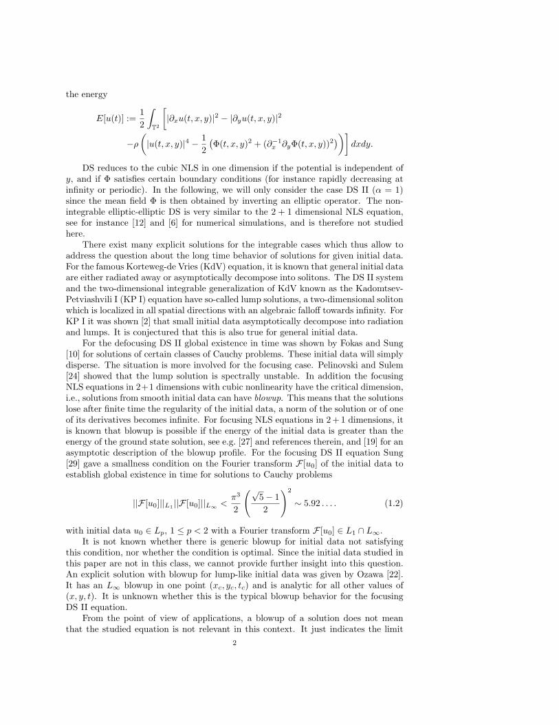
We choose Nx = Ny = 214 and Lx = Ly = 50, with ξ = 0, η = −1, z0 = 1 andc = 1. The large values for Lx and Ly are necessary to ensure that the solution issmall at the boundaries of the computational domain to reduce Gibbs phenomena.The difference for the mass of the lump and the computed mass on this periodicsetting is of the order of 6 ∗ 10−5. The initial data for t = −6 are propagated withNt = 1000 time steps until t = 6. In Fig. 2.1 contours of the solution at differenttimes are shown. Here and in the following we always show closeups of the solution.The actual computation is done on the stated much larger domain. In this paperwe will always show the square of the modulus of the complex solution for ease ofpresentation. The time dependence of the L2 norm of the difference between thenumerical and the exact solution can be also seen there.

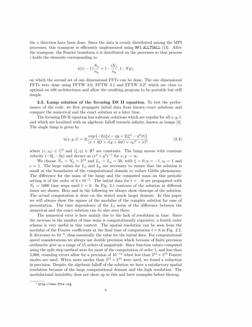
The numerical error is here mainly due to the lack of resolution in time. Sincethe increase in the number of time steps is computationally expensive, a fourth orderscheme is very useful in this context. The spatial resolution can be seen from themodulus of the Fourier coefficients at the final time of computation t = 6 in Fig. 2.2.It decreases to 10−6, thus essentially the value for the initial data. For computationalspeed considerations we always use double precision which because of finite precisionarithmetic give us a range of 15 orders of magnitude. Since function values computedusing the split step method were for most of the computation of order 1, and less than5,000, rounding errors allow for a precision of 10−14 when less than 215 × 215 Fouriermodes are used. When more modes than 215 × 215 were used, we found a reductionin precision. Despite the algebraic falloff of the solution we have a satisfactory spatialresolution because of the large computational domain and the high resolution. Themodulational instability does not show up in this and later examples before blowup.

1 http://www.fftw.org

6

Fig. 2.1. Contours of |u|2 on the left and a plot of ||uexact−unum||2 on the right in dependenceof time for the solution to the focusing DS II equation (1.1) for lump initial data (2.4).

Fig. 2.2. Fourier coefficients for the situation in Fig. 2.1 at t = 6.

3. Blowup for the quintic NLS in 1+1 dimensions and the focusing DSII. It is known that focusing NLS equations can have solutions with blowup, if thenonlinearity exceeds a critical value depending on the spatial dimension. For the 1+1dimensional case, the critical nonlinearity is quintic, for the 2 + 1 dimensional it iscubic, see for instance [28] and references therein. Thus the focusing DS II equationcan have solutions with blowup. In this section we will first study numerically blowupfor the 1 + 1 dimensional quintic NLS equation, and then numerically evolve initialdata for a known exact blowup solution to the focusing DS II equation due to Ozawa[22]. We discuss some peculiarities of the fourth order splitting scheme in this context.

3.1. Blowup for the quintic one-dimensional NLS. The focusing quinticNLS in 1 + 1 dimensions has the form

i∂tu+ ∂xxu+ |u|4u = 0, (3.1)

where u ∈ C depends on x and t (we consider again solutions periodic in x). Thisequation is not completely integrable, but assuming the solution is in L2, has conservedL2 norm and, provided the solution u ∈ H2, a conserved energy,

E[u] =∫

R

(12|∂xu|2 −

16|u|6)dx. (3.2)

It is known that initial data with negative energy blow up for this equation in finitetime, and that the behavior close to blowup is given in terms of a solution to an ODE,see [19].

7

As discussed in sect. 2.1, the splitting scheme we are using here has the propertythat the L2 norm is conserved. Thus the quality of the numerical conservation ofthe L2 norm gives no indication on the accuracy of the numerical solution. Howeveras discussed in [16], conservation of the numerically computed energy gives a validcriterion for the quality of the numerics: in general it overestimates the L∞ numericalerror by two orders of magnitude at the typically aimed at precisions.

If we consider as in [25] for the quintic NLS the initial data u0(x) = 1.8i exp(−x2),the energy is negative. We compute the solution with Lx = 5 and Nx = 215 withNt = 104 time steps. The result can be seen in Fig. 3.1 (to obtain more structure inthe solution after the blow up due to a less pronounced maximum, the plot on theleft was generated with the lower spatial resolution N = 212). The initial data clearly

21

01

2

0

0.1

0.20

100

200

300

xt

|u|2

Fig. 3.1. Solution to the focusing quintic NLS (3.1) for the initial data u0 = 1.8i exp(−x2)with N = 212 on the left and N = 215 on the right for t > tc.

get focused to a strong maximum, but the code does not break. We note that this isin contrast to other fourth order schemes tested for 1 + 1 dimensional NLS equationsin [16], which typically produce an overflow close to the blowup. But clearly thesolution shows spurious oscillations after the time tc ∼ 0.135. In fact the numericallycomputed energy, which will always be time-dependent due to unavoidable numericalerrors, will be completely changed after this time. We consider

∆E =∣∣∣∣1− E(t)

E(0)

∣∣∣∣ , (3.3)

where E(t) is the numerically computed energy (3.2) and get for the example inFig. 3.1 the behavior shown in Fig. 3.2. At the presumed blowup at tc ∼ 0.135 asin [25], the energy jumps to a completely different value. Thus this jump can andwill be used to indicate blowup. To illustrate the effects of a lower resolution in timeand space imposed by hardware limitations for the DS computations, we show thisquantity for several resolutions in Fig. 3.2. If a lower resolution in time is used asin some of the DS examples in this paper, the jump is slightly smoothed out. Butthe plateau is still reached at essentially the same time which indicates blowup. Thusa lack of resolution in time in the given limits will not be an obstacle to identify apossible singularity. The reason for this is the use of a fourth order scheme that allowsto take larger time steps. We will present computations with different resolutions toillustrate the steepening of the energy jump as above if this is within the limitationsimposed by the hardware.

We show the modulus of the Fourier coefficients for N = 212 and N = 215 beforeand after the critical time in Fig. 3.3. It can be seen that the solution is well resolved

8

0 0.05 0.1 0.15 0.212

10

8

6

4

2

0

2

4

t

log 10

E

Nt = 1000

Nt = 3000

Nt = 10000

0 0.05 0.1 0.15 0.215

10

5

0

5

t

log 10

E

Nt= 1000

Nt = 3000

Nt = 10000

Fig. 3.2. Numerically computed energy for the situation studied in Fig. 3.1 for N = 212 on theleft and N = 215 on the right for several values of Nt. At the blowup, the energy jumps.

before blowup in the latter case, and that the singularity leads to oscillations in theFourier coefficients. A lack of spatial resolution as for N = 212 in Fig. 3.3 triggers themodulation instability close to the blowup and at later times as can be seen from themodulus of the Fourier coefficients that increase for larger wavenumbers. Thereforewe always aim at a sufficient resolution in space even for times close to a blowup.After this time the modulation instability will be present in the spurious solutionproduced by the splitting scheme as we will show for an example.

500 0 5005

0

5t=0.134

log 1

0|v|

500 0 5005

0

5t=0.136

log 1

0|v|

500 0 5005

0

5

k

t=0.2

log 1

0|v|

4000 2000 0 2000 40002010010

t=0.134

log 1

0|v|

4000 2000 0 2000 40002010010

log 1

0|v| t=0.136

4000 2000 0 2000 40002010010

log 1

0|v|

k

t=0.2

Fig. 3.3. Fourier coefficients for the solution in Fig. 3.1 close to the critical and at a later timefor N = 212 on the left and N = 215 on the right for Nt = 104.

Remark 3.1. Stinis [25] has recently computed singular solutions to the focus-ing quintic nonlinear Schrodinger equation in 1 + 1 dimensions. This equation hassolutions in L∞L2 that may not be unique for given smooth initial data and that mayexhibit blowup of the L∞H1 norm. Following Tao [30], Stinis [25] has used a selectioncriteria to pick a solution after the blow up time of the L∞H1 norm. They suggestthat ‘mass’ is ejected (which means that the L2 norm is changed) at times where theL∞H1 norm blows up. The splitting scheme studied here in contrast produces a weaksolution with a different energy since the L2 norm conservation is built in.

3.2. Blowup in the Ozawa solution. For the focusing DS II equation, anexact solution was given by Ozawa [22] which is in L2 for all times with an L∞blowup in finite time. We can summarize his results as follows:

9

Theorem 3.1 (Ozawa). Let ab < 0 and T = −a/b. Denote by u(x, y, t) thefunction defined by

u(x, y, t) = exp(i

b

4(a+ bt)(x2 − y2)

)v(X,Y )a+ bt

(3.4)

where

v(X,Y ) =2

1 +X2 + Y 2, X =

x

a+ bt, Y =

y

a+ bt(3.5)

Then, u is a solution of (1.1) with

‖u(x, y, t)‖2 = ‖v(X,Y )‖2 = 2√π (3.6)

and

|u(t)|2 → 2πδ when t→ T. (3.7)

where δ is the Dirac measure.We thus consider initial data of the form

u(x, y, 0) = 2exp

(−i(x2 − y2)

)1 + x2 + y2

(3.8)

(a = 1 and b = −4 in (3.4)). As for the quintic NLS in 1 + 1 dimensions, we alwaystrace the conserved energy for DS II (1.1).

The computation is carried out with Nx = Ny = 215, Lx = Ly = 20, andNt = 1000 respectively Nt = 3000; we show the solution at different times in Fig. 3.4.The difference of the Ozawa mass and the computed L2 norm on the periodic settingis of the order of 9 ∗ 10−5.

The time evolution of maxx,y|u(x, y, t)|2 and the difference between the numerical

and the exact solution can be seen in Fig. 3.5 (the critical time tc is not on the showngrid, thus the solution is always finite on the grid points). The code continues to runafter the critical time, but the numerical solution obviously no longer represents theOzawa solution. The numerically computed energy jumps at the blow up time as canbe seen in Fig. 3.6. The Fourier coefficients at t = 0.13 are shown in Fig. 3.7. Despitethe Gibbs phenomenon the Fourier coefficients for the initial data decrease to 10−8.Spatial resolution is still satisfactory at half the blowup time.

Remark 3.2. The jump of the computed energy at blowup is dependent on suffi-cient spatial resolution as can be seen in Fig. 3.8 for the example of the quintic NLSof Fig. 3.2 and the Ozawa solution in Fig. 3.6. For low resolution blow-up can be stillclearly recognized from the computed energy, but the energy does not stay on the levelat blow-up.

4. Perturbations of the lump solution. In this section we consider pertur-bations of the lump solution (2.4). First we propagate initial data obtained from thelump after multiplication with some scalar factor. Then we consider a perturbationwith a Gaussian and a deformed lump.

4.1. Perturbation of the lump by rescaled initial data. We first considerrescaled initial data from the lump (2.4) denoted by ul

u(x, y,−6) = Aul,

10

Fig. 3.4. Solution to the focusing DS II equation (1.1) for t = 0.065 and t = 0.13 in the firstrow and t = 0.195 and t = 0.26 below for an initial condition of the form (3.8).

Fig. 3.5. Time evolution of max(|unum|2) and of ‖unum − uexact‖2 for the situation in Fig. 3.4.

where A ∈ R is a scaling factor. The computations are carried out withNx = Ny = 214

points for x× y ∈ [−50π, 50π]× [−50π, 50π] and t ∈ [−6, 6].

For A = 1.1, and Nt = 1000, we observe a blowup of the solution at tc ∼ 1.6.The time evolution of max

x,y|u(x, y, t)|2 and of the energy is shown in Fig. 4.1. The

maximum of |u|2 in Fig. 4.1 is clearly smaller than in the case of the Ozawa solution.This is due to the lower resolution in time which is used for this computation. Never-theless, the jump in the energy is obviously present. The Fourier coefficients at t = 0can be seen in Fig. 4.2. They again decrease by almost 6 orders of magnitude.

To illustrate the modulational instability at a concrete example, we show theFourier coefficients after the critical time in Fig. 4.3. It can be seen that the modulus

11

Fig. 3.6. Numerically computed energy E(t) and ∆E = |1−E(t)/E(0)| (3.3) for the situationin Fig. 3.4.

Fig. 3.7. Fourier coefficients of u at t = 0.13 for an initial condition of the form (3.8).

0 0.02 0.04 0.06 0.08 0.1 0.12 0.14 0.16 0.18 0.212

11

10

9

8

7

6

5

4

3

t

log 10

E

Fig. 3.8. Computed numerical energy for quintic NLS in Fig. 3.2 with N = 28 and for theOzawa solution in Fig. 3.6 with Nx = Ny = 212.

of the coefficients of the high wavenumbers increases instead of decreasing as to beexpected for smooth functions. This indicates once more that the computed solutionafter the blowup time has to be taken with a grain of salt.

For A = 0.9, the initial pulse travels in the same direction as the exact solution,but loses speed and height and is broadened, see Fig. 4.4. It appears that this mod-ified lump just disperses asymptotically. The solution can be seen in Fig. 4.5. Its

12

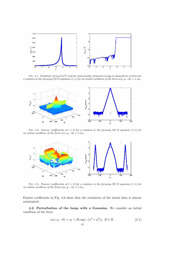
Fig. 4.1. Evolution of max(|u|2) and the numerically computed energy in dependence of time fora solution to the focusing DS II equation (1.1) for an initial condition of the form u(x, y,−6) = 1.1ul.

Fig. 4.2. Fourier coefficients at t = 0 for a solution to the focusing DS II equation (1.1) foran initial condition of the form u(x, y,−6) = 1.1ul.

Fig. 4.3. Fourier coefficients at t = 6 for a solution to the focusing DS II equation (1.1) foran initial condition of the form u(x, y,−6) = 1.1ul.

Fourier coefficients in Fig. 4.6 show that the resolution of the initial data is almostmaintained.

4.2. Perturbation of the lump with a Gaussian. We consider an initialcondition of the form

u(x, y,−6) = ul +B exp(−(x2 + y2)), B ∈ R. (4.1)13

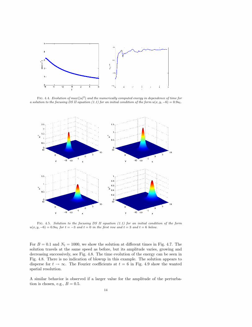
Fig. 4.4. Evolution of max(|u|2) and the numerically computed energy in dependence of time fora solution to the focusing DS II equation (1.1) for an initial condition of the form u(x, y,−6) = 0.9ul.

Fig. 4.5. Solution to the focusing DS II equation (1.1) for an initial condition of the formu(x, y,−6) = 0.9ul for t = −3 and t = 0 in the first row and t = 3 and t = 6 below.

For B = 0.1 and Nt = 1000, we show the solution at different times in Fig. 4.7. Thesolution travels at the same speed as before, but its amplitude varies, growing anddecreasing successively, see Fig. 4.8. The time evolution of the energy can be seen inFig. 4.8. There is no indication of blowup in this example. The solution appears todisperse for t → ∞. The Fourier coefficients at t = 6 in Fig. 4.9 show the wantedspatial resolution.

A similar behavior is observed if a larger value for the amplitude of the perturba-tion is chosen, e.g., B = 0.5.

14

Fig. 4.6. The Fourier coefficients at t = 0 of the solution to the focusing DS II equation (1.1)for an initial condition of the form u(x, y,−6) = 0.9ul.

Fig. 4.7. Solution to the focusing DS II equation (1.1) for an initial condition of the form (4.1)with B = 0.1 for t = −3 and t = 0 in the first row and t = 3 and t = 6 below.

4.3. Deformation of the Lump. We consider initial data of the form

u(x, y,−6) = ul(x, κy,−6), (4.2)

i.e., a deformed (in y-direction) initial lump in this subsection. The computations arecarried out with Nx = Ny = 214 points for x × y ∈ [−50π, 50π] × [−50π, 50π] andt ∈ [−6, 6].

For κ = 0.9, the resulting solution loses speed and width as can be seen in Fig. 4.10.Its height and energy grow, but both stay finite, see Fig. 4.11. It is possible that thesolution eventually blows up, but not on the time scales studied here.

15

Fig. 4.8. Evolution of max(|u|2) and of the energy in dependence of time for an initial conditionof the form (4.1) with B = 0.1.

Fig. 4.9. Fourier coefficients of u at t = 6 for an initial condition of the form (4.1) with B = 0.1.

−10 −5 0 5 10−10

−8

−6

−4

−2

0

2

4

6

8

10

Fig. 4.10. Contour plot for a solution to the focusing DS II equation (1.1) for an initialcondition of the form (4.2) with κ = 0.9 for different times.

The Fourier coefficients at t = 0 in Fig. 4.12 show the wanted spatial resolution.

For κ = 1.1, we observe the opposite behavior in Fig. 4.13. The solution travelswith higher speed than the initial lump and is broadened. The energy does not showany sudden change, see Fig. 4.14. It seems that the initial pulse will asymptoticallydisperse. The Fourier coefficients at t = 0 in Fig. 4.15 show the wanted spatial

16

Fig. 4.11. Evolution of max(|u|2) and the numerically computed energy in dependence of timefor the focusing DS II equation (1.1) for an initial condition of the form (4.2) with κ = 0.9.

−200 −150 −100 −50 0 50 100 150 200−8

−6

−4

−2

0

2

4

kx

log

10|v

(kx,

0)|

Fig. 4.12. Fourier coefficients of the solution to the focusing DS II equation (1.1) for an initialcondition of the form (4.2) with κ = 0.9 at t = 0.

resolution.

−15 −10 −5 0 5 10 15−10

−8

−6

−4

−2

0

2

4

6

8

10

Fig. 4.13. Contour plot for a solution to the focusing DS II equation (1.1) for an initialcondition of the form (4.2) with κ = 1.1 for different times.

5. Perturbations of the Ozawa solution. In this section we study as forthe lump in the previous section various perturbations of initial data for the Ozawasolution to test whether blowup is generic for the focusing DS II equation.

17

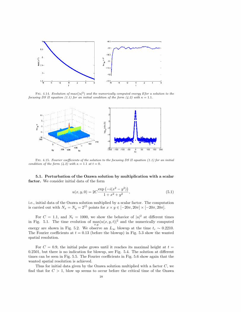
Fig. 4.14. Evolution of max(|u|2) and the numerically computed energy Efor a solution to thefocusing DS II equation (1.1) for an initial condition of the form (4.2) with κ = 1.1.

−200 −150 −100 −50 0 50 100 150 200−8

−6

−4

−2

0

2

4

kx

log

10|v

(kx,

0)|

Fig. 4.15. Fourier coefficients of the solution to the focusing DS II equation (1.1) for an initialcondition of the form (4.2) with κ = 1.1 at t = 0.

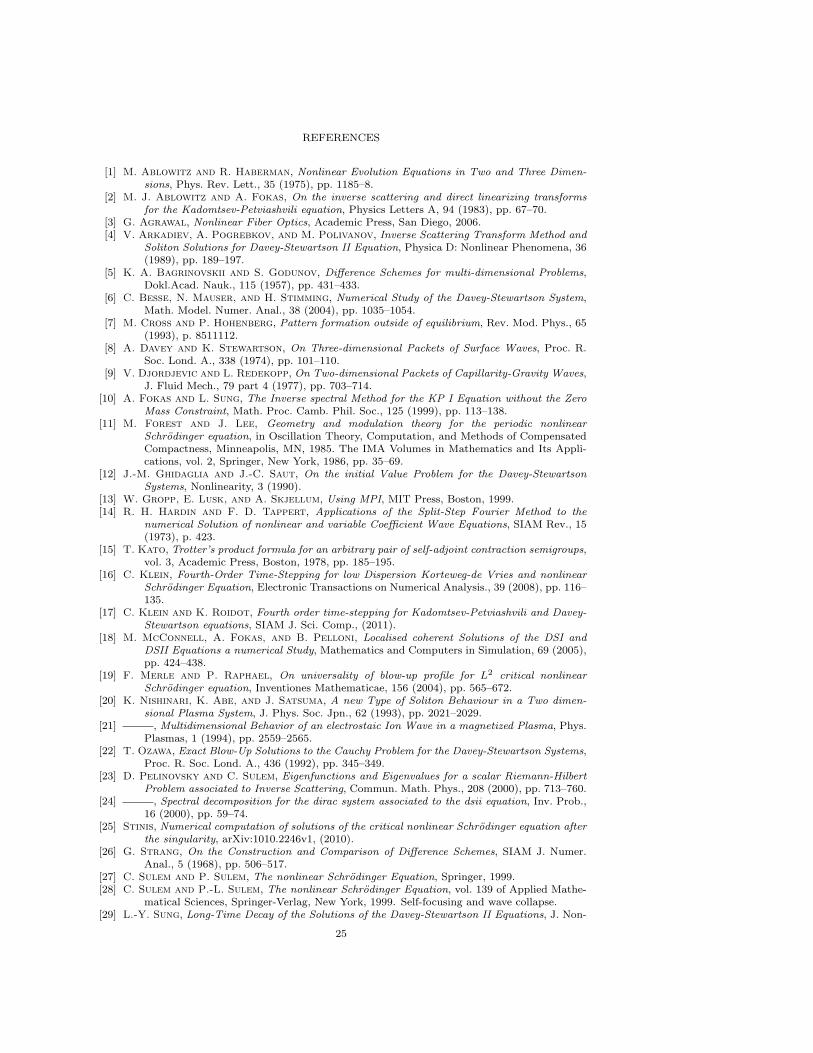
5.1. Perturbation of the Ozawa solution by multiplication with a scalarfactor. We consider initial data of the form

u(x, y, 0) = 2Cexp

(−i(x2 − y2)

)1 + x2 + y2

, (5.1)

i.e., initial data of the Ozawa solution multiplied by a scalar factor. The computationis carried out with Nx = Ny = 215 points for x× y ∈ [−20π, 20π]× [−20π, 20π].

For C = 1.1, and Nt = 1000, we show the behavior of |u|2 at different timesin Fig. 5.1. The time evolution of max

x,y|u(x, y, t)|2 and the numerically computed

energy are shown in Fig. 5.2. We observe an L∞ blowup at the time tc ∼ 0.2210.The Fourier coefficients at t = 0.13 (before the blowup) in Fig. 5.3 show the wantedspatial resolution.

For C = 0.9, the initial pulse grows until it reaches its maximal height at t =0.2501, but there is no indication for blowup, see Fig. 5.4. The solution at differenttimes can be seen in Fig. 5.5. The Fourier coefficients in Fig. 5.6 show again that thewanted spatial resolution is achieved.

Thus for initial data given by the Ozawa solution multiplied with a factor C, wefind that for C > 1, blow up seems to occur before the critical time of the Ozawa

18

Fig. 5.1. Solution to the focusing DS II equation (1.1) for an initial condition of the form (5.1)with C = 1.1 for t = 0.065 and t = 0.13 in the first row and t = 0.195 and t = 0.26 below.

Fig. 5.2. Evolution of max(|u|2) and the numerically computed energy for an initial conditionof the form (5.1) with C = 1.1.

solution, and for C < 1 the solution grows until t = 0.25 but does not blow up.Consequently the Ozawa initial data seem to be critical in this sense that data of thisform with smaller norm do not blow up.

5.2. Perturbation of the Ozawa solution with a Gaussian. We consideran initial condition of the form

u(x, y, 0) = 2exp

(−i(x2 − y2)

)1 + x2 + y2

+D exp(−(x2 + y2)). (5.2)

For D = 0.1 and Nt = 1000, we show the behavior of |u|2 at different times in Fig. 5.7.The time evolution of max

x,y|u(x, y, t)|2 is shown in Fig. 5.8. We observe a jump of the

19

−1000 −500 0 500 1000−5.5

−5

−4.5

−4

−3.5

−3

−2.5

−2

−1.5

−1

kx

log

10|v

(kx,0

)|

Fig. 5.3. Fourier coefficients of solution to the focusing DS II equation (1.1) for an initialcondition of the form (5.1) with C = 1.1 at t = 0.13.

Fig. 5.4. Evolution of max(|u|2) in dependence of time, for an initial condition of the form(5.1) with C = 0.9.

energy indicating blowup at the time tc ∼ 0.2332. The Fourier coefficients at tc = 0.13in Fig. 5.9 show that the wanted spatial resolution is achieved.

The same experiment with D = 0.5 appears again to show blow up, but at an earliertime tc ∼ 0.1659, see Fig. 5.10.

Thus the energy added by the perturbation of the form D exp(−(x2 + y2)) seemsto lead to a blowup before the critical time of the Ozawa solution. This means thatthe blowup in the Ozawa solution is clearly a generic feature at least for initial dataclose to Ozawa for the focusing DS II equation.

5.3. Deformation of the Ozawa solution. We study deformations of Ozawainitial data of the form

u(x, y, 0) = 2exp

(−i(x2 − (νy)2)

)1 + x2 + (νy)2

, (5.3)

i.e., a deformation in the y-direction. The computations are carried out with Nx =Ny = 215 points for x× y ∈ [−20π, 20π]× [−20π, 20π] and t ∈ [0, 0.26].

For ν = 0.9, we observe a maximum of the solution at t = 0.2441, see Fig. 5.11,followed by a second maximum, but there is no indication of a blowup. Energy con-servation is in principle high enough to indicate that the solution stays regular on the

20

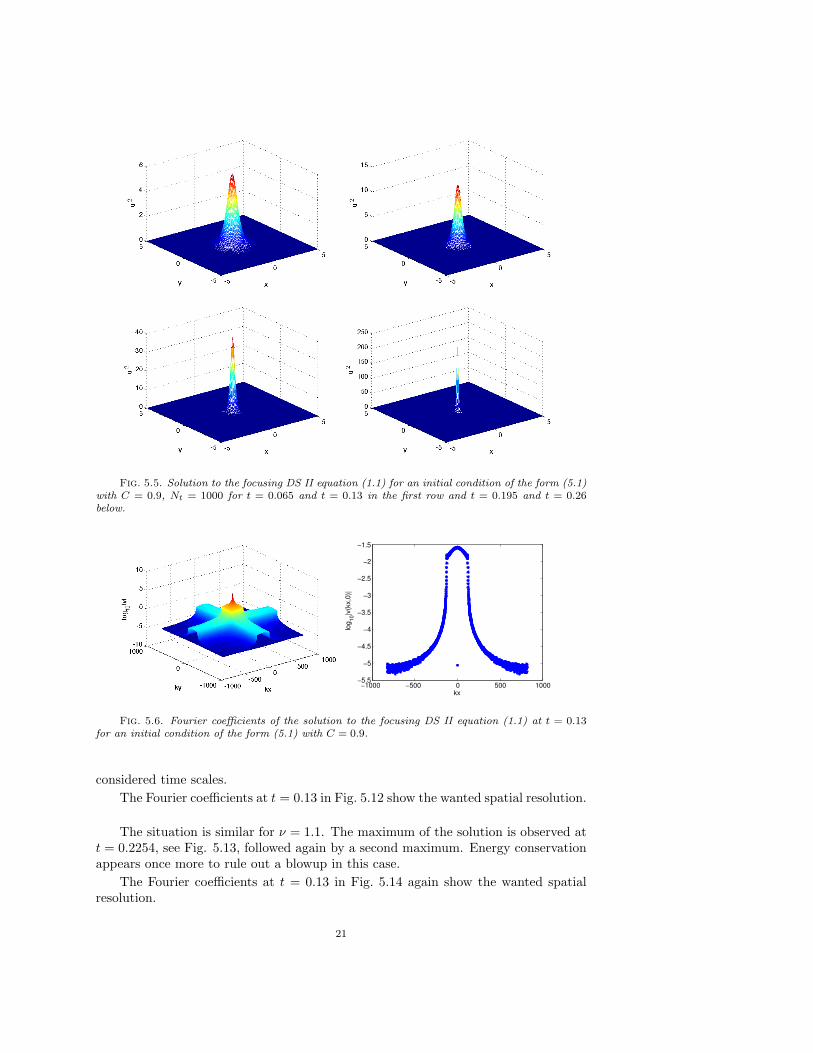
Fig. 5.5. Solution to the focusing DS II equation (1.1) for an initial condition of the form (5.1)with C = 0.9, Nt = 1000 for t = 0.065 and t = 0.13 in the first row and t = 0.195 and t = 0.26below.

−1000 −500 0 500 1000−5.5

−5

−4.5

−4

−3.5

−3

−2.5

−2

−1.5

kx

log

10|v

(kx,

0)|

Fig. 5.6. Fourier coefficients of the solution to the focusing DS II equation (1.1) at t = 0.13for an initial condition of the form (5.1) with C = 0.9.

considered time scales.The Fourier coefficients at t = 0.13 in Fig. 5.12 show the wanted spatial resolution.

The situation is similar for ν = 1.1. The maximum of the solution is observed att = 0.2254, see Fig. 5.13, followed again by a second maximum. Energy conservationappears once more to rule out a blowup in this case.

The Fourier coefficients at t = 0.13 in Fig. 5.14 again show the wanted spatialresolution.

21

Fig. 5.7. Solution to the focusing DS II equation (1.1) for an initial condition of the form (5.2)with D = 0.1 for t = 0.065 and t = 0.13 in the first row and t = 0.195 and t = 0.26 below .

Fig. 5.8. Evolution of max(|u|2) and the numerically computed energy in dependence of timefor the solution to the focusing DS II equation (1.1) for an initial condition of the form (5.2) withD = 0.1.

6. Conclusion. In this paper we have numerically studied long time behaviorand stability of exact solutions to the focusing DS II equation with an algebraicfalloff towards infinity. We have shown that the necessary resolution can be achievedwith a parallelized version of a spectral code. The spatial resolution as seen at theFourier coefficients was always well beyond typical plotting accuracies of the orderof 10−3. For the time integration we used an unconditionally stable fourth ordersplitting scheme. As argued in [16, 17], the numerically computed energy of thesolution gives a valid indicator of the accuracy for sufficient spatial resolution. Toensure the latter, we always presented the Fourier coefficients of the solution at atime before a singularity appeared. In addition we show here that the numerically

22

−1000 −500 0 500 1000−6

−5.5

−5

−4.5

−4

−3.5

−3

−2.5

−2

−1.5

kx

log

10|v

(kx,0

)|

Fig. 5.9. Fourier coefficients of the solution to the focusing DS II equation (1.1) at t = 0.13for an initial condition of the form (5.2) with D = 0.1.

Fig. 5.10. Evolution of max(|u|2) and the numerically computed energy for the solution to thefocusing DS II equation (1.1) for an initial condition of the form (5.2) with D = 0.5.

Fig. 5.11. Evolution of max(|u|2) and the numerically computed energy E in dependence oftime for a solution to the focusing DS II equation (1.1) for an initial condition of the form (5.3)with ν = 0.9.

computed energy indicates blowup by jumping to a different value in cases where thecode runs beyond a singularity in time.

After testing the code for exact solutions, the lump and the blowup solution byOzawa, we showed that both solutions are critical in the following sense: addingenergy to it leads to a blowup for the lump, and an earlier blowup time for the Ozawasolution. For initial data with less energy, no blowup was observed in both cases, theinitial data asymptotically just seem to be dispersed. This is in accordance with the

23

Fig. 5.12. Fourier coefficients of the solution to the focusing DS II equation (1.1) for an initialcondition of the form (5.3) with ν = 0.9 at t = 0.

Fig. 5.13. Evolution of max(|u|2) and the numerically computed energy E for a solution to thefocusing DS II equation (1.1) for an initial condition of the form (5.3) with ν = 1.1.

Fig. 5.14. Fourier coefficients of the solution to the focusing DS II equation (1.1) for an initialcondition of the form (5.3) with ν = 1.1 at t = 0.13.

conjecture in [18] that solutions to the focusing DS II equations either blow up ordisperse. In particular the lump is unstable against both blowup and dispersion, incontrast to the lump of the KP I equation that appears to be stable, see for instance[23]. Note that the perturbations we considered here test the nonlinear regime of thePDE for which so far no analytical results appear to be established.

24

REFERENCES

[1] M. Ablowitz and R. Haberman, Nonlinear Evolution Equations in Two and Three Dimen-sions, Phys. Rev. Lett., 35 (1975), pp. 1185–8.

[2] M. J. Ablowitz and A. Fokas, On the inverse scattering and direct linearizing transformsfor the Kadomtsev-Petviashvili equation, Physics Letters A, 94 (1983), pp. 67–70.

[3] G. Agrawal, Nonlinear Fiber Optics, Academic Press, San Diego, 2006.[4] V. Arkadiev, A. Pogrebkov, and M. Polivanov, Inverse Scattering Transform Method and

Soliton Solutions for Davey-Stewartson II Equation, Physica D: Nonlinear Phenomena, 36(1989), pp. 189–197.

[5] K. A. Bagrinovskii and S. Godunov, Difference Schemes for multi-dimensional Problems,Dokl.Acad. Nauk., 115 (1957), pp. 431–433.

[6] C. Besse, N. Mauser, and H. Stimming, Numerical Study of the Davey-Stewartson System,Math. Model. Numer. Anal., 38 (2004), pp. 1035–1054.

[7] M. Cross and P. Hohenberg, Pattern formation outside of equilibrium, Rev. Mod. Phys., 65(1993), p. 8511112.

[8] A. Davey and K. Stewartson, On Three-dimensional Packets of Surface Waves, Proc. R.Soc. Lond. A., 338 (1974), pp. 101–110.

[9] V. Djordjevic and L. Redekopp, On Two-dimensional Packets of Capillarity-Gravity Waves,J. Fluid Mech., 79 part 4 (1977), pp. 703–714.

[10] A. Fokas and L. Sung, The Inverse spectral Method for the KP I Equation without the ZeroMass Constraint, Math. Proc. Camb. Phil. Soc., 125 (1999), pp. 113–138.

[11] M. Forest and J. Lee, Geometry and modulation theory for the periodic nonlinearSchrodinger equation, in Oscillation Theory, Computation, and Methods of CompensatedCompactness, Minneapolis, MN, 1985. The IMA Volumes in Mathematics and Its Appli-cations, vol. 2, Springer, New York, 1986, pp. 35–69.

[12] J.-M. Ghidaglia and J.-C. Saut, On the initial Value Problem for the Davey-StewartsonSystems, Nonlinearity, 3 (1990).

[13] W. Gropp, E. Lusk, and A. Skjellum, Using MPI, MIT Press, Boston, 1999.[14] R. H. Hardin and F. D. Tappert, Applications of the Split-Step Fourier Method to the

numerical Solution of nonlinear and variable Coefficient Wave Equations, SIAM Rev., 15(1973), p. 423.

[15] T. Kato, Trotter’s product formula for an arbitrary pair of self-adjoint contraction semigroups,vol. 3, Academic Press, Boston, 1978, pp. 185–195.

[16] C. Klein, Fourth-Order Time-Stepping for low Dispersion Korteweg-de Vries and nonlinearSchrodinger Equation, Electronic Transactions on Numerical Analysis., 39 (2008), pp. 116–135.

[17] C. Klein and K. Roidot, Fourth order time-stepping for Kadomtsev-Petviashvili and Davey-Stewartson equations, SIAM J. Sci. Comp., (2011).

[18] M. McConnell, A. Fokas, and B. Pelloni, Localised coherent Solutions of the DSI andDSII Equations a numerical Study, Mathematics and Computers in Simulation, 69 (2005),pp. 424–438.

[19] F. Merle and P. Raphael, On universality of blow-up profile for L2 critical nonlinearSchrodinger equation, Inventiones Mathematicae, 156 (2004), pp. 565–672.

[20] K. Nishinari, K. Abe, and J. Satsuma, A new Type of Soliton Behaviour in a Two dimen-sional Plasma System, J. Phys. Soc. Jpn., 62 (1993), pp. 2021–2029.

[21] , Multidimensional Behavior of an electrostaic Ion Wave in a magnetized Plasma, Phys.Plasmas, 1 (1994), pp. 2559–2565.

[22] T. Ozawa, Exact Blow-Up Solutions to the Cauchy Problem for the Davey-Stewartson Systems,Proc. R. Soc. Lond. A., 436 (1992), pp. 345–349.

[23] D. Pelinovsky and C. Sulem, Eigenfunctions and Eigenvalues for a scalar Riemann-HilbertProblem associated to Inverse Scattering, Commun. Math. Phys., 208 (2000), pp. 713–760.

[24] , Spectral decomposition for the dirac system associated to the dsii equation, Inv. Prob.,16 (2000), pp. 59–74.

[25] Stinis, Numerical computation of solutions of the critical nonlinear Schrodinger equation afterthe singularity, arXiv:1010.2246v1, (2010).

[26] G. Strang, On the Construction and Comparison of Difference Schemes, SIAM J. Numer.Anal., 5 (1968), pp. 506–517.

[27] C. Sulem and P. Sulem, The nonlinear Schrodinger Equation, Springer, 1999.[28] C. Sulem and P.-L. Sulem, The nonlinear Schrodinger Equation, vol. 139 of Applied Mathe-

matical Sciences, Springer-Verlag, New York, 1999. Self-focusing and wave collapse.[29] L.-Y. Sung, Long-Time Decay of the Solutions of the Davey-Stewartson II Equations, J. Non-

25

linear Sci., 5 (1995), pp. 433–452.[30] T. Tao, Global existence and uniqueness results for weak solutions of the focusing mass-critical

nonlinear Schrodinger equation, Analysis and PDE, 2 (2009), pp. 61–81.[31] F. Tappert, Numerical Solutions of the Korteweg-de Vries Equation and its Generalizations by

the Split-Step Fourier Method, Lectures in Applied Mathematics, 15 (1974), pp. 215–216.[32] H. Trotter, On the Product of Semi-Groups of Operators, Proceedings of the American

Mathematical Society, 10 (1959), pp. 545–551.[33] P. White and J. Weideman, Numerical Simulation of Solitons and Dromions in the Davey-

Stewartson System, Math. Comput. Simul., 37 (1994), pp. 469–479.[34] H. Yoshida, Construction of higher Order symplectic Integrators, Physics Letters A, 150

(1990), pp. 262–268.

26