numerical study a flow around a heated finite cylinder and

Numerical study a flow around a heated finite cylinder and mounted

vertically on a flat plate

Hamza GOUIDMI1, 2, Razik BENDERRADJI1,3, Abdelhadi BEGHIDJA1

1Laboratory of Renewable Energies and Sustainable Development (LERDD), Frères Mentouri

University, Constantine1-Algeria 2Mohamed El-Bachir El-Ibrahimi University, Bordj Bou Arréridj- Algeria

3Mohamed Boudiaf University, M’Sila- Algeria

[email protected]

Abstract: - Flow around a finite end cylinder mounted vertically on a flat plate and thermally heated is

simulated numerically by the Large-Scale Simulation (LES) approach. The flow is in subcritical regime

circulate with a velocity U∞=0.54m/s corresponding a Reynolds number ReD=2.2x104. The boundary

condition of Neumann is imposed on the surface of the cylinder, which is reflected by a density of the heat flux

is = 600W/m2, for an aspect ratio H/D=5.This simulation induces a complex structure of the flow behind the

cylinder, in particular the appearance of vortices and recirculation zones ahead and behind it. The results

obtained give a clear comparison with those found experimentally and numerically of Guillermo Palau-

Salvador et al. [2], that were carried out its work in the case of adiabatic flow.

Key-Words: - Heated Cylinder, Vortex Structures, Mixed Convection.

Abbreviations:

TFC: Horseshoe vortex.

VKV: Von Kàrmàn vortex

KHV: Whirlwind of Kelvin Helmholtz

BV: wake whirlpools

TM: Marginal vortices

Re: Reynolds Number

Nu: Nusselt Number

Pr : Prandtl Number

1 Introduction These phenomena are classical but they exist and

encountered in industrial applications, especially

combined phenomena between thermal and dynamic

transfer, such as cylindrical buildings, piles or

cooling towers placed in the atmospheric boundary

layer where it interacts with the wind, cooling fins

of computer processors, rods in various technical

equipment such as fuel or central rods in nuclear

power plants and open channels. The flows around

the thermally heated free-end cylinders add other

nascent complex secondary vortices above and

behind them, because they are three-dimensional

nature and very unstable character. However,

globally, several parameters affecting these vortex

phenomena, we quote: The Reynolds number, the

aspect ratio defined by H/D (H is the height of the

cylinder and D the diameter) and the shape of the

cylinder...etc. It has for example the effect of aspect

ratio on the overall structure of the nascent vortices

in Fig.1 driven by Kawamura et al. [1]. Many

experimental and numerical scientific works have

treated these phenomena, such as the works of [1],

[2], [3], [4], [5]. The technological development of

computer hardware has improved the calculations of

complex problems and compared them with

experience.

Flow around a circular cylinder at a free end

thermally heated and vertically mounted on a flat

plate for an aspect ratio H/D=5 is simulated

numerically by the LES approach, using the Fluent

6.3 calculation code. However, the study is carried

out with a heat flux imposed on the surface of the

cylinder is 600W/m2. This work is based on

experimental studies of [2] and [3] by adding the

thermal study we heating the cylinder. We will

WSEAS TRANSACTIONS on HEAT and MASS TRANSFER Hamza Gouidmi, Razik Benderradji, Abdelhadi Beghidja

E-ISSN: 2224-3461 66 Volume 14, 2019

mailto:[email protected]

analyze and treat it after the obtained results, such as

the average and fluctuating fields as well as the

average Nusselt number.

Fig.1: Vortices structures for two different aspect ratios,

Boizumault et al. [1].

2 Configuration and numerical model 2.1 Test configuration

The geometry used in numerical simulations is

shown in Fig. 2. It is a three-dimensional cylinder of

circular section mounted on a horizontal wall. The

cylinder has a diameter D= 0.04 m and a height H=

0.2 m. Its aspect ratio AR=H/D= 5. The length of

the computation domain is L=1.52 m, its height is

0.4 m and its depth is 0.56 m. The center of the

cylinder is placed as a reference direct orthogonal, is

located 0.32m downstream of the entrance face.

Then, the blocking factor (S/So), defined by the ratio

between the surfaces of the cylinder projected on

the input surface is about 3.5%. The boundary

condition imposed on the surface of the cylinder is

verified by the Neumann condition, which is

signified by a heat flux density equal 600W/m2.

Fig. 2: Geometry and dimensions of the configuration.

The fluid used is water, passing through the

cylinder with a uniform velocity U∞=0.54m/s giving

a Reynolds number based on the diameter of the

cylinder of the order of Re = 2.2x104. The numerical

simulations were carried out on a 3D control space

with implicit temporal discretization of the second

order. The dimensioning and the inlet flow

parameters are shown in Table 1.

Table 1 : Dimensions and input parameters D (m) H (m) U∞ (m/s) AR S/So Re

0.04 0.2 .54 H/D=5 0.035 2.2.104

2.2 Numerical model

2.2.1 Description

The flow is considered incompressible in physical

properties constant. The calculation scheme chosen

makes it possible to solve the averaged filtered

Navier-Stokes equations (spatial averaging)

implicitly to find the temperature, the velocity and

the pressure, such as conservation equations of

mass, momentum and energy.

2.2.2 Large Eddy Simulation; LES

In the assumptions of viscous incompressible flow,

the continuity, momentum and energy equations

filtered take the following form:

(1)

(2)

(3)

Where ρ is the density of the fluid, ν is the

kinematic viscosity, is the filtered temperature,

is the filtered velocity, is the filtered pressure.

and are the heat flux and stress tensor in the

subgrid scale, respectively, defended by the

following relations:

(4)

(5)

The standard Smagorinsky model is used in this

work to modeled the stresses and heat flux in the

subgrid scale (SGS).


E-ISSN: 2224-3461 67 Volume 14, 2019

The origin of this model is based on the

assumption of equilibrium between production and

dissipation for small scales. In this model, the

stresses and heat fluxes on the subgrid scale are

calculated with the dynamic approach of Germano

et al. [6] as modified by Lilly et al. [7], which

models the anisotropic part of the term SGS, which

is written as follows:

(6)

(7)

Where, is the subgrid scale viscosity, is the

subgrid scale diffusivity, is the strain tensor rate

defined as:

(8)

The subgrid scale viscosity is defined by:

(9)

is the filter scale considered as the cubic root of

the volume of the finite volume cell and Cs is the

Smagorinsky constant.

The value of the constant model in this study

was 0.1. In the same way , the subgrid scale

diffusivity, αt, is defined as follows:

(10)

Where Prt = 0.6 is the the subgrid scale Prandtl

number. The Smagorinsky model is widely used in

body bluff simulations (see [8] and [9]). It has also

used the modeling of unresolved flows in

simulations of heat transfer problems, see reference

[10].

2.2.3 Mesh of the computational domain In order to solve the Navier-Stokes equations,

FLUENT 6.3 software based on the finite volume

approach. For this configuration, the mesh used is

structured quadrilateral multi-blocks was made

using the software GAMBIT 2.4, presented in Fig.3.

We get in this mesh 1185506 nodes or 1146000

cells hexahedral mesh well refined near the walls of

the cylinder.

To the numerical calculation, the velocity-

pressure coupling is achieved by Coupled algorithm.

The interpolation of the pressure is carried out by

the interpolation scheme "body force weighted" and

the terms of the transport equations is carried out by

the interpolation scheme "Bounded Central

Differencing" with relaxation factors in explicit

form. The equation of energy is discretized by the

interpolation scheme "Second Order Upwind".

All results, including the spectra (Fig.11) indicate

that the resolution obtained is sufficient.

The time steps were such that the maximum

number CFL was 0.83 and the Strouhal number St=

0.2. In this case we can calculate the frequency

control of the convergence by the relation f

(St.U)/D which must be equal to 2.7. Therefore,

the flow time calculate is 8.88s with a time step Δt =

0.0148s.

Fig.3: Non-regular mesh by block of the computational

domain is 1146000 cells.

3 Validation of the results The comparison of the results of the numerical

simulation with those of the experiment of G. P.

Salvador et al. [2], is shown in Fig.4.

Fig.4: Distribution of mean longitudinal velocities in

the median plane (z = 0) at y/h= 0.6.


E-ISSN: 2224-3461 68 Volume 14, 2019

The average longitudinal velocity profile flow 

in the median plane along the line y/h=0.6 obtained

by LES gives a good agreement with the

experimental velocity profile.

This comparison gives a validation of the

numerical model LES used. So; the following

calculations will be based on the chosen numerical

model.

4 Results and discussion In this section, we will analyze the qualitative and

quantitative results interesting obtained from the

numerical simulation, including the instantaneous

and average velocity curves, the mean Nusselt

number curves, the contours of the Q criterion and

the turbulence statistics of the first and the second

order.

4.1 The Dynamic analysis 4.1.1 Comparison of the velocity profiles

In the present study, we compare the mean and

fluctuating longitudinal, lateral and vertical velocity

profiles obtained by LES with those experimentally

measured [2] (that its worked was carried out in

the case of adiabatic flow where the absence of

the thermal effect) along the longitudinal and

vertical as well as transversal lines where the flow

regime is supercritical with a number Reynolds

ReD=2.2x104 and for a density of heat flux imposed

on the wall on the surface cylinder ϕ=600 W/m2.

Fig.5, shows the profiles of the longitudinal and

vertical mean velocities u and v along the line’s

y/h=0.2 and 0.6, respectively, in the median plane.

The mean longitudinal profiles indicates a clear

deceleration upstream of the cylinder, then they are

zero at the passage of the cylinder and then they

continue to decrease downstream thereof to the

boundary of the recirculation zone. At the exit of

this zone, the velocity profiles return to take the

positive values in the wake zone. Whereas, for the

vertical profiles <v>, at the upstream of cylinder

they are zero, which translates the flow is purely

developed along the axis ox, then they are zero

during the passage of the cylinder, then downstream

of it, they take a negative value.

These profiles are marked a maximum value at

an abscissa x/D=2 in all cases whether experimental

or simulation by LES. The upstream of cylinder, all

profiles are given a good agreement with the

experimental of [1], while downstream of it, they

differ slightly from these, exclusively the

longitudinal velocity profile at height y/h=0.6,

which gave a better comparison. These different are

marked in the zone behind the cylinder (in the wake

zone).

Fig.6, shows the fluctuating velocities profiles of

longitudinal and vertical, u and v, in the median

plane along line y/h=0.2 and 0.6, respectively. It can

be seen that the LES calculation is not badly

compared with the experimental at the height

y/h=0.6, whereas at y/h=0.2, there was some

difference especially in the margin of y/h=0.9 to 2.2.

For the maximum turbulence rate, was marked at

x/D=0.25 in the all calculations whether by

experience or by LES.

Fig.7, shows the evolutions of the averages and

fluctuations longitudinal and vertical velocities

profiles in the median plane (Z = 0) along the line

x/D=1.We find that the profiles of the average

velocities obtained by LES give an agreement with

the experimental of [1].Whereas, the velocity

fluctuation profiles obtained by LES are compared

well with the experience of [1]. In the near wall the

longitudinal and vertical velocity fluctuations are

given rates of 25% and 10%, respectively.

Fig.8, shows the evolutions of the averages and

fluctuating longitudinal and lateral velocity profiles

along the lateral line at x/D=1.5 from the center and

downstream of the cylinder in a height y/h=0.6. We

observe that the velocity profiles obtained by LES

whether longitudinal or lateral are similar with those

experimental results.

Fig.5: Evolutions of longitudinal and vertical averages

velocities in the median plane at heights y/h=0.2 and 0.6.


E-ISSN: 2224-3461 69 Volume 14, 2019

Fig.6: Evolutions of fluctuating velocities profiles of

longitudinal and vertical in the median plane at heights

y/h=0.2 and 0.6.

Fig.7: Evolutions of the averages and fluctuating

longitudinal and vertical velocities along the line x/D=1

in the median downstream of the cylinder.

Fig.8: Evolutions of the averages and fluctuating profiles

of the longitudinal and lateral velocities along the lateral

line at x/D=1.5 from the center and downstream of the

cylinder and in a height y/h=0.6.

4.1.2 Pressure coefficient profiles

The pressure coefficients obtained during our

simulations are compared to the theoretical function,

see the Fig.9. These coefficients are given for a

perfect flow to vary according to the function Cp=1-

4sin2θ.

In order to analyze the obtained results, the theory

indicate that the detachment zone is in the range

(60° θ<120°). At the leading edge of the cylinder we

find values of Cp equal 0.6, which are corresponding

to the same gaits, see the fig.9. They translate the

points of stagnation (point of stops), where the

pressure is maximum which is signified the zero

velocity (the concordance of the Bernoulli

equation).

In this figure the pressure coefficients plot for two

heights y/h=0.5 and 0.8. We an increase of the

absolute values of the pressure coefficient up to the

maximum values CPmax=1.78 and 1.99 at y/h=0.2

and 0.6, respectively, corresponding the value of

θ=77.1°, and then they are constant in the remaining

margin.

The angle of detachment which results in the point

of separation is of order of θS=102°, it is a value

belongs in the zone of separation (60°<θS<120°).

So, the LES turbulence model gives a very good

agreement for these margins of θ. These offsets of

the average pressure coefficients are directly related

to the type of boundary conditions imposed.

Fig.9: Evolutions of the theoretical pressure coefficient

profiles for a perfect flow vary by the function Cp = 1-

4sin2θ and our result at ϕ= 600W/m2 at a height y/h= 0.5.

4.1.3 Visualization of mean and fluctuating

fields 4.1.3.1 In the longitudinal center plane

Fig. 10 and 11, show the streamlines followed by

the average longitudinal velocity fields dimensioned

by the upstream velocity of fluid, streamwise and

spanwise velocities fluctuations fields which are

plotted in the longitudinal center plane of the

cylinder (z=0). It is found that the mean streamwise

velocity is important above the shear layer,

which is translated in an acceleration of the flow,

and a recirculation zone behind the cylinder has

appeared and is limited by a separation line. While,


E-ISSN: 2224-3461 70 Volume 14, 2019

streamwise and spanwise velocities fluctuations are

important in the recirculation zone of the flow,

behind the cylinder and close to the middle thereof,

respectively. These fields flow are marked with a

maximum value near to 0.3 m/s which has been

found experimentally by [2].

Fig.10: Mean streamlines and streamwise velocity fields

on the mid-transverse plane (z/D = 0).

Fig.11: Root mean square of the streamwise (u') and

spanwise (w') fluctuations on the mid-transverse plane

(z/D = 0).

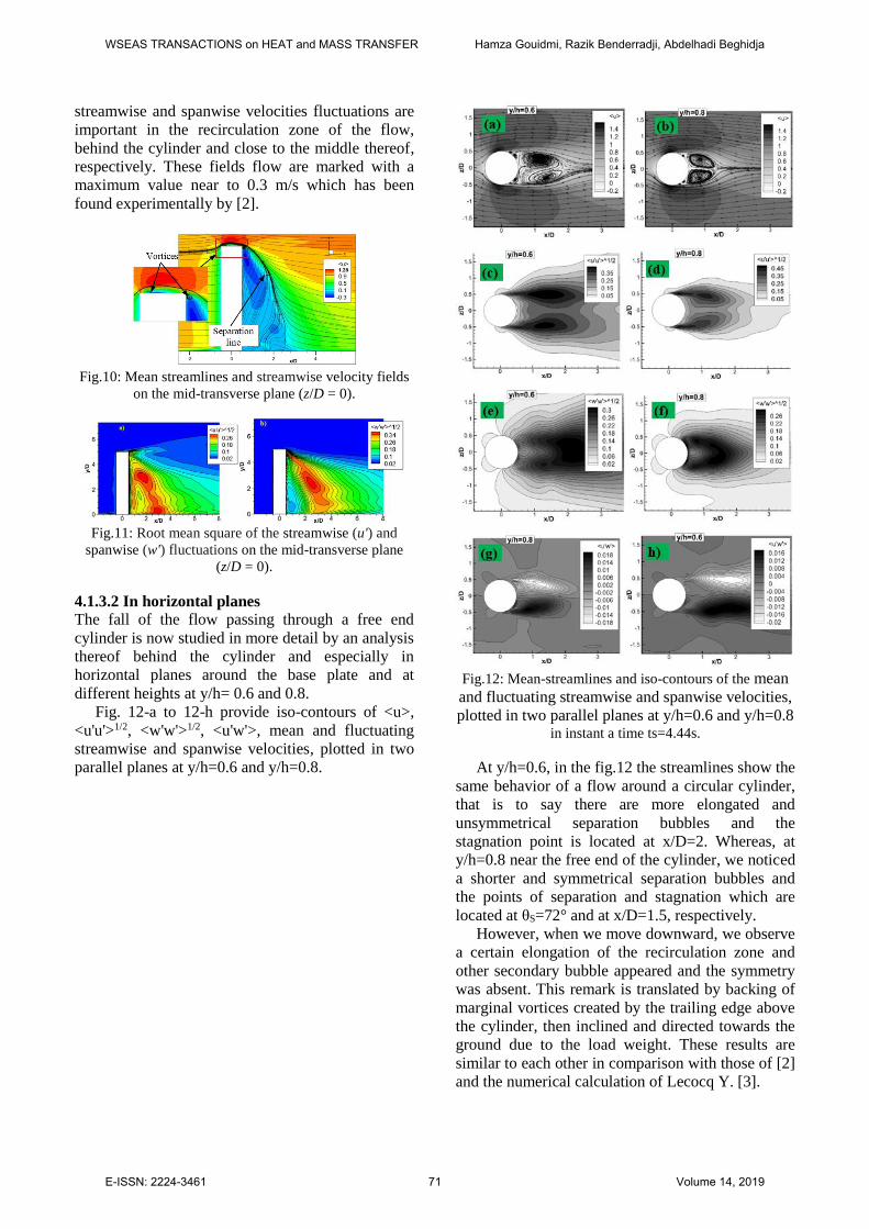
4.1.3.2 In horizontal planes

The fall of the flow passing through a free end

cylinder is now studied in more detail by an analysis

thereof behind the cylinder and especially in

horizontal planes around the base plate and at

different heights at y/h= 0.6 and 0.8.

Fig. 12-a to 12-h provide iso-contours of ,

<u'u'>1/2, <w'w'>1/2, <u'w'>, mean and fluctuating

streamwise and spanwise velocities, plotted in two

parallel planes at y/h=0.6 and y/h=0.8.

Fig.12: Mean-streamlines and iso-contours of the mean

and fluctuating streamwise and spanwise velocities,

plotted in two parallel planes at y/h=0.6 and y/h=0.8 in instant a time ts=4.44s.

At y/h=0.6, in the fig.12 the streamlines show the

same behavior of a flow around a circular cylinder,

that is to say there are more elongated and

unsymmetrical separation bubbles and the

stagnation point is located at x/D=2. Whereas, at

y/h=0.8 near the free end of the cylinder, we noticed

a shorter and symmetrical separation bubbles and

the points of separation and stagnation which are

located at θS=72° and at x/D=1.5, respectively.

However, when we move downward, we observe

a certain elongation of the recirculation zone and

other secondary bubble appeared and the symmetry

was absent. This remark is translated by backing of

marginal vortices created by the trailing edge above

the cylinder, then inclined and directed towards the

ground due to the load weight. These results are

similar to each other in comparison with those of [2]

and the numerical calculation of Lecocq Y. [3].


E-ISSN: 2224-3461 71 Volume 14, 2019

4.1.4 Vortices structures of the flow In this work, the numerical simulations of flow

around a cylinder are carried out by the LES

approach in a subcritical regime at Reynolds

number ReD=2.2x104 in the range 300≤ReD≤ 2·105.

The flow passing through a free end cylinder

causing a pressure difference between the base and

the edge thereof induced by a flow deflection and

the creation of marginal vortices, also called

secondary flow. These behaviors may be to cause:

An expansion of the area downstream of the

cylinder translated by formations vortex and the

extent of the area near wake following the

intensity of this deflection (when the Strouhal

number decreases).

A non-existent vortex shedding for low aspect

ratio values; the figure 2.16 shows that the

secondary flow then becomes the main flow.

The criteria presented above pose a major

difficulty for the configuration study presenting the

situations of the flow around a free end cylinder. We

present in the rest of this paragraph criteria based on

the tensor components of velocity gradient .

Criteria for the function Q

The definition of a vortex given by Hunt et al.

(1988) calling the second invariant Q of . Q is

then defined: .

Or; Sij and Ωij represents the symmetrical and

asymmetrical portions of the velocity gradient

tensor. So:

.

Thus, physically, the regions where Q is negative

represent the regions where the vorticity is greater

than the deformation. This criterion will therefore be

more efficient than the norm of vorticity alone in the

near-wall zones.

The criterion based on the norm of the vorticity

offers the very parasitized views by the strong shear

regions. Following observations that were found or

represented by Kawamura et al. [1], P. G. Salvador

et al. [2], Y. Lecocq [3] and others, we privileged

the use of the criterion Q for the visualization of

coherent structures in our simulations.

Basing on the instantaneous characteristics of the

solution obtained by the LES calculation. An

overview of the flow is shown in fig.13. We present

in the first place the iso-surface of the criterion-Q,

such that Q = 20. It is found that the overall

behavior of the flow is clear.

Fig.13, shows the presence of a horseshoe

tourbillon, noted TFC1, marginal vortices, TM,

Trailing Vortices, denoted TV 1 and 2, Von Karman

vortices (VKV), Kelvin-Helmholtz vortices (KHV)

and Hairpin vortices (TEC).

We observe a sudden deflection fluid just after

the cylinder. Marginal vortices, TM, are driven to

y/h<1 and probably intersect with Von Karman

vortices (VKV). We can also see the nascent

horseshoe vortex upstream of the cylinder and then

the separation of its legs when the fluid passes the

cylinder. These structures will be seen in more

detail in Figs. 15 on sectional planes.

Still in FIG. 13, the Kelvin-Helmholtz vortices

(KHV) originating from the detachment of the

lateral boundary layers are observed. The axis of

these vortices is almost rectilinear on the portion

y/h∈ (1/4, 3/4) with respect to the axis of the

cylinder in the plane (xoz) and is inclined outside.

The curvature of these vortices is certainly related to

the increase of the velocity when y/H>3/4 and not to

the slope of the velocity profile imposed at the

entrance of the domain of computation. End

eddies greatly influence the wake of flow for

this aspect ratio. The temporal evolution of the instantaneous flow

is shown in FIG. 10 in the constant margin non-

dimensional time Δt*= (Δt.u∞)/D=10. This figure

represents the whole of the three-dimensional (3D)

flow, in particular, the vortices formed around the

side and behind the cylinder visualized using the

iso-surfaces of the of the wheel invariant<Q> = 20

to left and <Q> = 50 on the right. These vortex

structures, globally, give the same images as

observed in Figure 1 plotted by Boizumault et al.

[1].


E-ISSN: 2224-3461 72 Volume 14, 2019

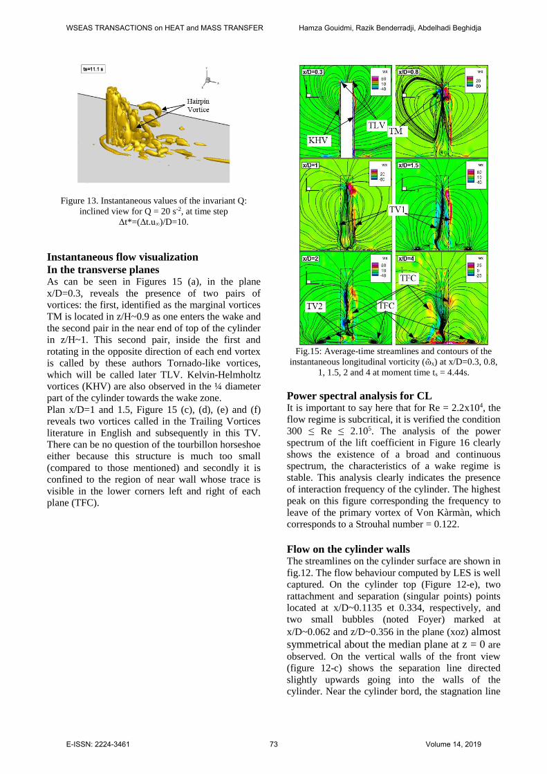
Figure 13. Instantaneous values of the invariant Q:

inclined view for Q = 20 s-2, at time step

Δt*=(Δt.u∞)/D=10.

Instantaneous flow visualization

In the transverse planes As can be seen in Figures 15 (a), in the plane

x/D=0.3, reveals the presence of two pairs of

vortices: the first, identified as the marginal vortices

TM is located in z/H~0.9 as one enters the wake and

the second pair in the near end of top of the cylinder

in z/H~1. This second pair, inside the first and

rotating in the opposite direction of each end vortex

is called by these authors Tornado-like vortices,

which will be called later TLV. Kelvin-Helmholtz

vortices (KHV) are also observed in the ¼ diameter

part of the cylinder towards the wake zone.

Plan x/D=1 and 1.5, Figure 15 (c), (d), (e) and (f)

reveals two vortices called in the Trailing Vortices

literature in English and subsequently in this TV.

There can be no question of the tourbillon horseshoe

either because this structure is much too small

(compared to those mentioned) and secondly it is

confined to the region of near wall whose trace is

visible in the lower corners left and right of each

plane (TFC).

Fig.15: Average-time streamlines and contours of the

instantaneous longitudinal vorticity (ῶx) at x/D=0.3, 0.8,

1, 1.5, 2 and 4 at moment time ts = 4.44s.

Power spectral analysis for CL It is important to say here that for Re = 2.2x104, the

flow regime is subcritical, it is verified the condition

300 ≤ Re ≤ 2.105. The analysis of the power

spectrum of the lift coefficient in Figure 16 clearly

shows the existence of a broad and continuous

spectrum, the characteristics of a wake regime is

stable. This analysis clearly indicates the presence

of interaction frequency of the cylinder. The highest

peak on this figure corresponding the frequency to

leave of the primary vortex of Von Kàrmàn, which

corresponds to a Strouhal number = 0.122.

Flow on the cylinder walls The streamlines on the cylinder surface are shown in

fig.12. The flow behaviour computed by LES is well

captured. On the cylinder top (Figure 12-e), two

rattachment and separation (singular points) points

located at x/D~0.1135 et 0.334, respectively, and

two small bubbles (noted Foyer) marked at

x/D~0.062 and z/D~0.356 in the plane (xoz) almost

symmetrical about the median plane at z = 0 are

observed. On the vertical walls of the front view

(figure 12-c) shows the separation line directed

slightly upwards going into the walls of the

cylinder. Near the cylinder bord, the stagnation line


E-ISSN: 2224-3461 73 Volume 14, 2019

splits into a current line fan due to the end effect.

The side view (fig.12-b), shows the separation line

at a fairly constant angle of 84.3° relative the axis

ox. This line is therefore largely vertical and in the

upper end is slightly curved towards the median

plane (z = 0). In the back and below ends region,

there is a vortex and a singular points node-like of

separation, there the motion is directed upwards,

downwards and sideways.

Fig.16: Power spectral density function of lift on the

finite-length cylinder. The straight dotted line has a slope

of -5/3 in the logarithmic curve.

Figure 17. Streamlines of flow on the surfaces cylinder:

a) Rear face, b) Side face, c) Front face, d) Above face

and near the ground (e) for H/D=5.

Thermal analysis

Température fields

In heat transfer by forced convection, the thermal

field is combined by the dynamic field. Thus, the

number of Nusselt can be calculated according to

the characteristics of the dynamic regime

considered. It is possible to find global relations

involving the Reynolds number with the Prandtl

number according to the following correlation:

where represents the mean of the Nusselt

number. One can also find local correlations i.e.

involving for example the angle reflecting the

thickening of the mechanical boundary layer (sum

of the dynamic and thermal limit layers), according

to Eckert [15] the number of Nusselt in this case is

written:

Finally, it is possible to characterize the heat

transfer over the entire circumference of the

cylinder and thus take into account the separation of

the boundary layer which is followed by the

appearance of a medium flow recirculation zone

which intervene. on its surface.

Sanitjai & Goldstein [16] distinguish three zones

in which different correlations can be applied.

- The first one is the one where the Nusselt

number is monotonically decreasing as a function

of θ due to the thickening of the boundary layer

until its detachment, , equation (13). At

this position the observed minimum is an overall

minimum. According to Bailer et al. [17] who

performed numerical simulations at Re = 200 and

Re = 2000, it seems that the heat transfer in this

first zone is independent of time.

- The second zone is between the detachment and

the second minimum, local this time,

equation (14). There is an increase in heat transfer

that is proportional to the Reynolds number.

- In the third zone, there is an increase in the

Nusselt number due to vortex shedding,

, equation (15). The last two zones

are dependent on the Reynolds number but also on

the incident turbulence.

On the contrary, tangentially to the wall, the

speed of the water increases along the front face

from the point of attack, then decreases along the

rear face. When the velocity gradient is zero, the

boundary layer separates from the wall and

convective heat exchange reaches a minimum. The

0.122

-5/3


E-ISSN: 2224-3461 74 Volume 14, 2019

separate flow area at the rear of the cylinder appears

to be turbulent. These general flow behaviors are

well observed in the velocity profiles indicated

above.

Nusselt Numbers profiles The effect of the heating of a cylinder on the water

flow is less important, due of the difference between

the reference temperature flow and the average

surface temperature calculated from the Neumann

condition. Y. Lecocq [3] has shown that there is a

major effect of the heating on the overall structure

of the flow behind the cylinder. For this reason, the

Nusselt number can be presented in FIG. 13 for two

height levels at y/h=0.2,0.5, 0.6 and 1 as a function

of the rotation angle θ of the cylinder.

It can be seen that, for y/h=1, the evolutions of

the profiles are based on the typical image of the

flow around a circular cylinder, while for the others

nearly they conform between (-112° and 100°). In

addition, when moving downwards, the angles are

taken the positive values of (100° to 180°) and from

(-112° to -180°) the evolutions are superimposed on

each other with lower Nusselt values.

Figure 18. Evolutions of the average Nusselt

number profiles at different heights y/h=0.2,0.5, 0.6

and 1 as a function of the rotation angle θ of the

cylinder.

Instantaneous average and fluctuating

temperature fields

Figures 19 and 20 show the fields of the

instantaneous average and fluctuating temperatures

in different cross-sectional planes, x/D=0.3, 0.8, 1,

1.5, 2 and 4 and for a density of the heat flux

imposed on the cylinder of 600 W/m2. It can be seen

in both figures and for all transverse planes that the

two types of temperature are marked with maximum

values near the ground. When moving towards the

rear of the cylinder, it is observed that the heat is

diffused well towards the ground in an almost

symmetrical manner.

These observations due to the strong deflection

of the water down which fell not far from the

cylinder in the wake. This fluid is also responsible

for transporting heat from the cylinder to the wake

zone, where heat transfer can be defined by forced

convection.

Figure 19: Contours of instantaneous average température

<T> in y-z planes at 6 consecutive streamwise locations:

x/D=0.3, 0.8, 1, 1.5, 2 and 4 in instant a time ts = 11.84s.

Fig.20: Contours of instantaneous fluctuating température

T’ in y-z planes at 6 consecutive streamwise locations:

x/D=0.3, 0.8, 1, 1.5, 2 and 4 in instant a time ts = 11.84s.

To give another explanation for the convective

heat transfer, we will present the fields of the mean

and fluctuating surface temperatures of the cylinder

in Figure 16. It is found that the average and


E-ISSN: 2224-3461 75 Volume 14, 2019

fluctuating temperatures have marked maximum

values close to 295.25 K and 1.6 K, respectively

near ground.

Fig.21: Evolutions of the average and fluctuating

surface temperatures fields of the cylinder.

4 Conclusion Large Scale Simulation (LES) has been used

successfully to study the viscous incompressible

flow around a circular cylinder thermally heated on

its surface by an imposed heat flux density ϕ =

600W/m2. It is mounted vertically on an adiabatic

flat wall and with an aspect ratio AR=H/D=5.

The obtained results by LES have made it

possible to analysed and present the necessary fields

flow, such as, mean and fluctuating velocities fields

in the three directions, as well as the instantaneous

fields which are presented by iso-surfaces of the

criterion Q. Finally, the average Nusselt number

presenting for different heights. From this work it

can be seen that forced convection heat exchange is

well carried out. Generally, the results obtained are

consistent with those found experimentally and

numerically.

References: [1] Kawamura, T., Hiwada M., Hibino T, Mabuchi I.,

and Kamuda M, Flow around a finite circular

cylinder in a flat plate. (1984) Bull. JSME, 27(232)

:2412–2151.

[2] P. Salvador G., Thorsten S.,Jochen F., Michael K.,

Wolfgang R.et al, Large Eddy Simulations and

Experiments of Flow around Finite-Height

Cylinders, (2009) Flow Turbulence Combust,

84:239–275, 21 August.

[3] Lecocq Y., contribution à l’analyse et à la

modélisation des écoulements turbulents en régime

de convection mixte –application à l’entreposage

des d´déchets radioactifs, (2008) thèse de Doctorat

de l’université de Poitiers.

[4] Norberg C., An experimental investigation of the

flow around a circular cylinder: influence of aspect

ratio, (1994) J . Fluid Mech., nol. 258, p p . 287-

316.

[5] Persillon H, Braza M., Physical analysis of the

transition to turbulence in the wake of a circular

cylinder by three-dimensional Navier-Stokes

simulation, (1998) J. Fluid Mech.vol. 365, pp.23-88.

[6] Germano, M., Piomelli, U., Moin, P., Cabot, W.H.,

A dynamic subgrid-scale eddy viscosity model,

(1991) Phys. Fluids3,1760-1765.

[7] Lilly D.K., A proposed modification of the Germano

subgrid-scale closure method, (1992) Phys. Fluids

4, 633–635.

[8] Hemida H., Large-Eddy Simulation of the Flow

around Simplified High-Speed Trains under Side

Wind Conditions, (2006) thesis of Lic. Of Engng,

Division of Fluid Dynamics, Universit de Chalmers

of Technology, Göteborg, Sweden.

[9] Krajnović S., Davidson L., Flow around a Simplified

car, Part (1): Large-Eddy Simulation", (2005)

Journal of Fluid Engineering, Vol. 127, pp. 907-

918.

[10] Barhaghi D., Davidson L., Karlsson R., Large

Eddy Simulation of Natural Convection Boundary

Layer on a Vertical Cylinder, Selected paper, (2006)

International Journal of Heat and Fluid Flow, to

appear.

[11] T. Rödiger, H. Knauss, U. Gaisbauer,

E. Krämer, Pressure and Heat Flux Measurements

on the Surface of a Low-Aspect-Ratio Circular

Cylinder Mounted on a Ground Plate, 96 New

Results in Numerical and Experimental Fluid

Mechanics VI: Contributions to the 15th

STAB/DGLR Symposium Darmstadt, Germany,

121-126. 2006.

[12] Kappler, M.: Experimentelle Untersuchung der

Umströmung von Kreiszylindern mit ausgeprägt

dreidimensionalen Effekten. Ph.D. thesis, University

of Karlsruhe. http://digbib.ubka.uni-karlsruhe. De

/volltexte/12232002 (2002).

[13] Donnert, G.D., Kappler, M., Rodi, W.:

Measurement of tracer concentration in the flow of

finite-height cylinders. Jornal of Turbulence. 8(33),

1–18 (2007).

[14] Etzold, F., Fiedler, H. The near-wake structure

of a cantilevered cylinder in a cross flow. Zeitschrift

für Flugwissenschaften 24, S. 77-82 1976.

[15] E. R. G. Eckert. Die berechnung des

wärmeüberganges in der laminaren

renzschicht umströmter körper. VDI-Foshungsheft 416, 1942.

[16] S. Sanitjai and R. J. Goldstein. Forced

convection heat transfer from circular cylinder

in crossflow to air and liquids. Int. J. of Heat

and Mass transfer, 47 :4795–4805, 2004.

[17] F. Bailer, P. Tochon, J.-M. Grillot, and P.

Mercier. Simulation numérique de

l’écoulement et transfert de chaleur autour d’un

cylindre. In Elsevier, editor, Revue Générale de

Thermique, volume 36, pages 744–754. 1997


E-ISSN: 2224-3461 76 Volume 14, 2019

http://digbib/

numerical study a flow around a heated finite cylinder and

Documents