Contents lists available at ScienceDirect

Ocean Engineering

journal homepage: www.elsevier.com/locate/oceaneng

Numerical studies on added resistance and motions of KVLCC2 in head seasfor various ship speeds

Mingyu Kima,⁎, Olgun Hizirb, Osman Turana, Atilla Incecika

a Department of Naval Architecture, Ocean and Marine Engineering, University of Strathclyde, 100 Montrose Street, Glasgow G4 0LZ, UKb Ponente Consulting Ltd., Ipswich, Suffolk IP2 0EL, UK

A R T I C L E I N F O

Keywords:Added resistanceShip motionsPotential flowCFDKVLCC2

A B S T R A C T

In this study, numerical simulations for the prediction of added resistance and ship motions at various shipspeeds and wave steepnesses for the KVLCC2 are presented. These are calculated using URANS CFD and 3-Dpotential methods, both in regular head seas. Numerical analysis is focused on the added resistance and thevertical ship motions for a wide range of wave conditions at stationary, operating and design speeds. Firstly, thecharacteristics of the CFD and the 3-D potential method are presented. Simulations of various wave conditionsat design speed are used as a validation study, and then simulations are carried out at stationary and operatingspeed. Secondly, unsteady wave patterns and time history results of the added resistance and the ship motionsare simulated and analysed at each ship speed using the CFD tool. Finally, the relationship between the addedresistance and the vertical ship motions is studied in detail and the non-linearity of the added resistance andship motions with the varying wave steepness are investigated. Systematic studies of the numericalcomputations at various ship speeds are conducted as well as the grid convergence tests, to show that thenumerical results have a reasonable agreement with the available EFD results.

1. Introduction

Now more than ever, the reduction of ship pollution and emissions,maximisation of energy efficiency, enhancement of safety requirementsand minimization of operational expenditure are required and sought.Traditionally, only ship resistance and propulsion performance in calmwater were considered at the ship design stage and during the designprocess even though recently the hull form has been optimised for aspecific range of draught and speed ranges considering the operationalprofile (Kim and Park, 2015). However, when a ship advances in aseaway, she requires additional power in comparison with the powerrequired in calm water due to weather effects and ship operatingconditions. This degradation of the ship performance in a seaway,which is reported to be about 15–30% of the power required in calmwater (Arribas, 2007) is accounted for by the application of a “SeaMargin” onto the total required engine power, and a value of 15% istypically used. The added resistance due to waves is one of the majorcomponents affecting ship performance in a seaway. Therefore, accu-rate prediction of the added resistance in waves is essential to evaluatethe additional power requirement, to assess the full environmentalimpact and to design ships with high fuel efficiency in realisticoperating conditions. This can also be combined with other operational

measures to ensure greater efficiency, such as voyage planning andweather routing. Additionally, correct estimation and understanding ofthe ship motions are crucial to ensure safe navigation. Regardinginternational regulations, the Marine Environment ProtectionCommittee (MEPC) of the International Maritime Organization(IMO) issued new regulations to improve the energy efficiency levelof ships and to reduce carbon emissions. These regulations include theEnergy Efficiency Design Index (EEDI) as a mandatory technicalmeasure for new ships and the Energy Efficiency OperationalIndicator (EEOI) which is related to ship voyage and operationalefficiency as a technical measure for ships in service. Recently, the shipspeed reduction coefficient (fw) has been proposed and is underdiscussion for the calculation of EEDI in representative sea states(IMO, 2012; ITTC, 2014). Moreover, guidelines for determiningminimum propulsion power to maintain the manoeuvrability of a shipin adverse weather conditions (IMO, 2013) have been developed forsafe manoeuvring.

The added resistance and ship motion problem in waves has beenwidely studied by conducting experiments and numerical simulationsusing potential flow theory and Computational Fluid Dynamics (CFD)approaches. There are two major analytical approaches in potentialflow methods which are used to calculate the added resistance: the far-

http://dx.doi.org/10.1016/j.oceaneng.2017.06.019Received 15 November 2016; Received in revised form 3 May 2017; Accepted 7 June 2017

⁎ Corresponding author.E-mail address: mingyu.kim@strath.ac.uk (M. Kim).

Ocean Engineering 140 (2017) 466–476

Available online 16 June 20170029-8018/ © 2017 The Authors. Published by Elsevier Ltd. This is an open access article under the CC BY license (http://creativecommons.org/licenses/BY/4.0/).

MARK

field method and the near-field method. The far-field method is basedon the added resistance computed from the wave energy and themomentum flux generated by a ship and is evaluated across a verticalcontrol surface of infinite radius surrounding the ship. This methodwas first introduced by Mauro (1960) using the Kochin function whichconsists of radiating and diffracting wave components. This methodwas also applied to predict the added resistance and wave drift of shipsby Joosen (1966) and Newman (1967) respectively. Later on, the far-field method based on the radiated energy approach was proposed byGerritsma and Beukelman (1972) to predict the added resistance inhead seas. This approach became popular in strip theory programs dueto its easy implementation. Recently, Liu et al. (2011) solved the addedresistance problem with a quasi-second-order approach using thehybrid Rankine Source-Green function method considering the asymp-totic and empirical methods which improved the results in short waves.Another numerical approach is the near-field method which estimatesthe added resistance by integrating the hydrodynamic pressure on thebody surface. This method was first introduced by Havelock (1937)who used the Froude-Krylov approach to calculate hull pressures. Thenear-field method was enhanced by Faltinsen et al. (1980) based on thedirect pressure integration approach. Salvesen et al. (1970) introduceda simplified asymptotic method based on 2-D strip theory to overcomethe deficiency of this approach in short waves. Kim et al. (2007) andJoncquez (2009) formulated the added resistance based on theRankine panel method using a time-domain approach with B-splinefunctions and investigated the effects of the Neumann-Kelvin (NK) andDouble Body (DB) linearization schemes on the added resistancepredictions. Recently, Kim et al. (2012) formulated the added resis-tance using a time-domain B-spline Rankine panel method based onboth near-field and far-field methods in addition to the NK and DBlinearization schemes for the forward speed problem. In the presentstudy, the 3D linear potential flow method is applied to predict the shipmotions and the added resistance using the NK linearization schemeand near-field method in regular waves due to more accurate predic-tion of ship motions and added resistance of blunt ships compared tothe DB method (Kim and Shin, 2007).

Recently as computational facilities have become more powerfuland more accessible, CFD tools are now commonly used to predictadded resistance and ship motions. It has advantages over potentialcodes as it can deal directly with large amplitude ship motions and withnonlinear flow phenomena such as breaking waves and green water,without explicit approximations and empirical values. Deng et al.(2010), El Moctar et al. (2010) and Sadat-Hosseini et al. (2010)predicted the added resistance of KVLCC2 in head waves using CFDtools as presented at the Gothenburg (2010), SIMMAN (2014) andSHOPERA (2016) Workshops. Following that, Guo et al. (2012)investigated the added resistance, ship motions and wake flow ofKVLCC2 in head waves with systematic validation and verification ofthe numerical computation and Sadat-Hosseini et al. (2013) predictedthe added resistance and motions for KVLCC2 using an in-house codeCFDSHIP-IOWA which is based on a Unsteady Reynolds-AveragedNavier-Stokes (URANS) approach. In addition to the studies on theprediction of added resistance and ship motions in waves, there havebeen subsequent investigations on how to reduce the added resistanceby modifying the hull form. Park et al. (2014) and Kim et al. (2015)modified the fore body of KVLCC2 to reduce the added resistance inwaves. Additionally, based on CFD simulations, Kim et al. (2014)modified the bulbous bow of a containership to optimize the hull formfor both operating conditions in calm water and waves. There have alsobeen investigations concerning the increase in the required power andthe ship speed loss due to waves. Kwon (2008) predicted the ship speedloss using semi-empirical model considering wind, motions anddiffraction resistance while Prpić-Oršić and Faltinsen (2012) investi-gated the ship speed loss and CO2 emission considering addedresistance due to waves and the propeller performance in actual sea,and (Kim et al., 2016) presented a reliable methodology to estimate the

added resistance and the ship speed loss of a containership due to windand waves in random seas.

In the study presented in this paper, the numerical simulations forthe prediction of the added resistance and the ship motions forKVLCC2 in regular head waves are carried out using URANS and 3-D potential flow methods. The results obtained are validated with theavailable experimental data and during the study grid convergencetests are also carried out for the CFD approach. The added resistanceand the vertical ship motions are examined for various wave conditionsat the design and operating speeds as well as at the stationarycondition. Unsteady wave patterns and the time history results of theresistance and vertical ship motions in waves are simulated using aCFD tool. The relationship between the added resistance and the shipmotions for various ship speeds and wave steepness are investigatedincluding the viscous effects and non-linear phenomena such as greenwater on deck.

2. Ship particulars and coordinate system

All calculations of the added resistance and ship motions have beenperformed for KVLCC2, which represents the second variant of theVLCC-type vessel developed by the Korea Research Institute of Shipsand Ocean Engineering (KRISO) which is one of benchmark hull formsused to study seakeeping problems by researchers. The principalparticulars of the KVLCC2 are given in full scale in Table 1.

For CFD simulations, a model scale vessel without appendagesusing a scale ratio of 1/80 is employed in the calculations.

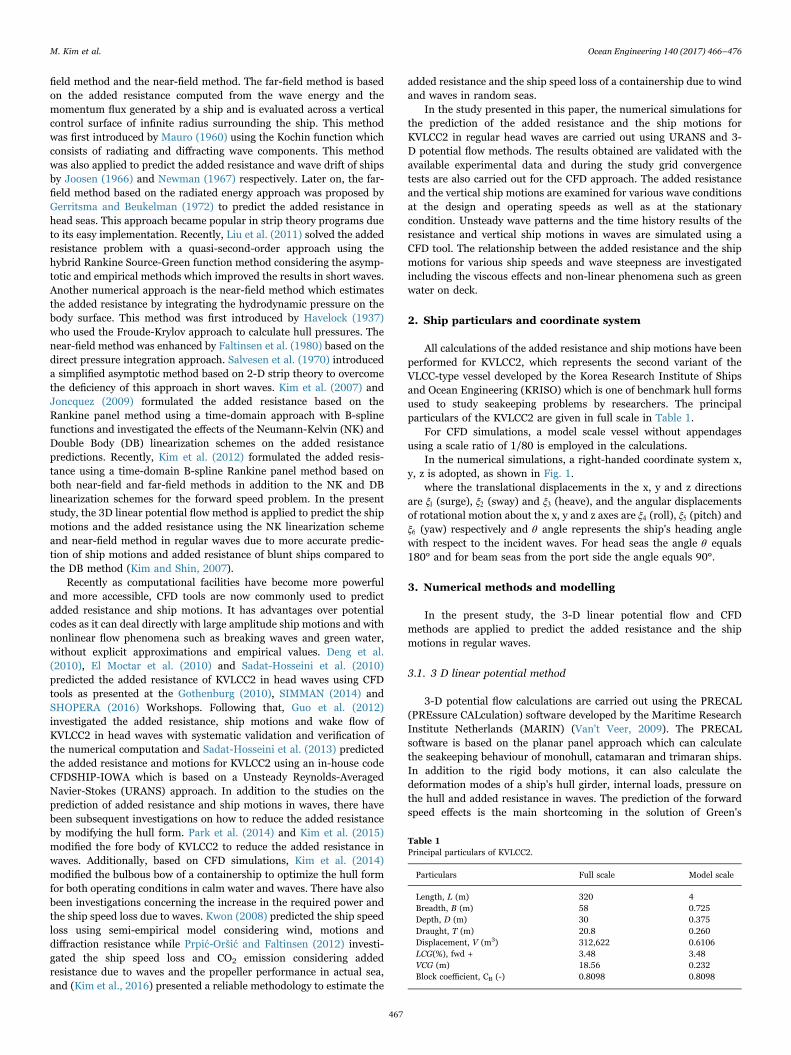
In the numerical simulations, a right-handed coordinate system x,y, z is adopted, as shown in Fig. 1.

where the translational displacements in the x, y and z directionsare ξ1 (surge), ξ2 (sway) and ξ3 (heave), and the angular displacementsof rotational motion about the x, y and z axes are ξ4 (roll), ξ5 (pitch) andξ6 (yaw) respectively and θ angle represents the ship's heading anglewith respect to the incident waves. For head seas the angle θ equals180° and for beam seas from the port side the angle equals 90°.

3. Numerical methods and modelling

In the present study, the 3-D linear potential flow and CFDmethods are applied to predict the added resistance and the shipmotions in regular waves.

3.1. 3 D linear potential method

3-D potential flow calculations are carried out using the PRECAL(PREssure CALculation) software developed by the Maritime ResearchInstitute Netherlands (MARIN) (Van't Veer, 2009). The PRECALsoftware is based on the planar panel approach which can calculatethe seakeeping behaviour of monohull, catamaran and trimaran ships.In addition to the rigid body motions, it can also calculate thedeformation modes of a ship's hull girder, internal loads, pressure onthe hull and added resistance in waves. The prediction of the forwardspeed effects is the main shortcoming in the solution of Green's

Table 1Principal particulars of KVLCC2.

Particulars Full scale Model scale

Length, L (m) 320 4Breadth, B (m) 58 0.725Depth, D (m) 30 0.375Draught, T (m) 20.8 0.260Displacement, V (m3) 312,622 0.6106LCG(%), fwd + 3.48 3.48VCG (m) 18.56 0.232Block coefficient, CB (-) 0.8098 0.8098

M. Kim et al. Ocean Engineering 140 (2017) 466–476

467

functions due to the complex numerical integration process on thewaterline sections. Numerical methods need to be implemented tosolve the Boundary Value Problem (BVP) in the presence of forwardspeed and the Green's functions need to be satisfied both for the Free-Surface Boundary Condition (FSBC) and the Body Boundary Condition(BBC). PRECAL is a 3-D source-sink frequency domain code capable ofsolving the forward speed linear BVP using the Approximate ForwardSpeed (AFS) and the Exact Forward Speed (EFS) methods. In the AFSmethod the BVP is solved using zero-speed Green's functions and thenforward speed corrections are applied to the BVP equations. It ispossible to use the Lid panel method (Lee and Sclavounos, 1989) wherewaterplane area (Lid) panels are used to suppress the occurrence of theirregular frequencies in the BVP solutions. In the EFS method, exactforward speed Green's functions are used to solve the forward speedBVP, but in the PRECAL software Lid panel method can only beapplied to the AFS formulation. In this study, forward speed shipmotions are solved using the AFS formulation due to its fast and

accurate results (Hizir, 2015). The added resistance is calculated usingthe near-field method based on direct pressure integration over themean wetted hull surface, using the second-order forces to calculatewave drift forces while the first-order forces and moments are

Fig. 1. Vessel coordinate system.

Fig. 2. Mesh and boundary conditions.

Table 2Test cases for grid convergence (λ/L = 1.2, H/λ = 1/60, Vs = 15.5 knots).

Grid name Case no. Mesh λ/Δx H/Δz Te/Δt

G1 C1F Fine 140 28 362G2 C10 Base 100 20 256 (28)G3 C1C Coarse 70 14 181

Cell number

RA

W/(ρ

gA2 B

2 /L)

0 2E+06 4E+06 6E+06 8E+062

4

6

8

Fig. 3. Grid convergence test for the added resistance (Vs = 15.5 knots, λ/L = 1.2, H/ λ= 1/60, model scale).

Fig. 4. Time histories of total resistance, heave and pitch motions in waves (Case: C10,model scale).

M. Kim et al. Ocean Engineering 140 (2017) 466–476

468

calculated to solve the ship motions. The total pressure is divided intofour components which originate from the relative water height,incident wave velocities, the pressure gradient and the rotation timesinertial terms. The added resistance force due to waves (ΔRwave) iscalculated in the time domain as shown in Eq. (1).

∫

∫

∫

R

ρ ϕ ϕ n ds

ρ α ϕ ϕ n ds

ρg ζ α n dl M X

Δ =

− ∇→

⋅∇→ →

− (→ ⋅∇→

) + ∇→

⋅∇→ →

+ ( − ) → + Ω→

×⎯→⎯ ̈

wave

H

Hϕ

t

wl

(1) (1) (0)

(1) ∂∂

(1) (0)

12

(1)3(1) 2 (0) (1) (1)

0

0

(1)

⎡

⎣

⎢⎢⎢⎢⎢⎢

⎛⎝⎜

⎞⎠⎟

⎤

⎦

⎥⎥⎥⎥⎥⎥(1)

where the first integral is the water velocity contribution, the secondintegral is the pressure gradient contribution, the third integral is therelative wave height contribution and the last term is the rotation timesinertia contribution. The indices stand for the order of the forces in theforce contribution formulations. H0 represents the mean position of theship, α⎯→(1) represents the first order translation and rotation vector, n⎯→(0)

is the zeroth order normal vector calculated on the mean positionvessel wetted surface and Ω(1) is the first order rotation vector. In orderto derive the added resistance equation in the frequency domain, anoscillatory description of motion and flow is introduced and the steadyflow contribution is neglected. The added resistance in the frequencydomain is formulated by:

∫

∫

∫

ϕ

i ϕ

g M

ΔR =

− ρ ∇→

n→ ds

− ρ ( α→ ⋅∇→

)( ω ∇→

) n→ ds

+ ρ ζ n→ dl − ω Ω→

× X→

wave

H(1) 2 (0)

H(1)

e(1) (0)

12 wl

(1) 2 (0)e2 (1) (1)

0

0

⎡

⎣

⎢⎢⎢⎢⎢⎢

⎤

⎦

⎥⎥⎥⎥⎥⎥ (2)

In order to evaluate the added resistance forces, all components inthe integrals are defined in perturbation series. A small parameter (ε) isintroduced to represent the quantities in the perturbation series. Theperturbation series expansion of the relative wave height and thevelocity potential can be formulated as shown in Eqs. (3) and (4):

ζ ζ εζ ε ζ Ο ε= + + + ( )(0) (1) 2 (2) 3 (3)

ϕ ϕ εϕ ε ϕ Ο ε= + + + ( )(1) 2 (2) 3 (4)

where zeroth order quantities are time independent and are assumed tobe small to satisfy the linearized free-surface condition. For the samereason, time-dependent parts of the series are also assumed to besmall.

In added resistance calculations, only the mean values of the forcesand moments are of interest. First-order quantities such as motions,velocities, accelerations etc. have a mean value of zero when the wave isgiven by an oscillatory function with a mean value of zero. However,

Table 3Test cases at design speed (15.5 knots).

Case no. Vs [knots] Wavelength(λ/L)

Waveheight(H)[m]

Wavesteepness(H/λ)

fe [Hz](model)

Te [sec.](model)

C00 15.5 Calm water – – – –

C10 1.20 6.40 1/60 0.7560 1.3227C11 0.50 2.67 1.3293 0.7523C12 0.75 4.00 1.0186 0.9818C13 1.00 5.33 0.8476 1.1798C14 1.40 6.40 0.6872 1.4552C15 1.60 7.47 0.6332 1.5793

λ/L

ξ 3/A

0 0.5 1 1.5 2 2.50

0.5

1

1.5

2EFD (Osaka University, 2010)EFD (Lee et al., 2013)Rankine panel method (Seo et al., 2014)Present (3-D Potential Method)Present (CFD)

λ/L

ξ 5/k

A

0 0.5 1 1.5 2 2.50

0.5

1

1.5

2EFD (Osaka University, 2013)EFD (Lee et al., 2013)Rankine panel method (Seo et al., 2014)Present (3-D Potential Method)Present (CFD)

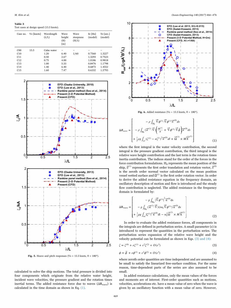
Fig. 5. Heave and pitch responses (Vs = 15.5 knots, θ = 180°).

λ/L

RA

W/(ρ

gA2 B

2 /L)

0 0.5 1 1.5 2 2.50

2

4

6

8

10EFD (Lee et al. 2013, H/L=0.015)EFD (Sadat-Hosseini, 2013)Rankine panel method (Seo et al., 2014)CFD (Sadat-Hosseini, 2013)Present (3-D Potential Method, H=2m)Present (CFD, H/λ=1/60)

Fig. 6. Added resistance (Vs = 15.5 knots, θ = 180°).

M. Kim et al. Ocean Engineering 140 (2017) 466–476

469

second-order quantities such as added resistance have a non-zero meanvalue therefore in order to calculate the added resistance, second-orderforces and moments need to be calculated. In the present study, in thecalculation of added resistance only the constant part (mean value) ofthe added resistance is taken into account while the slowly oscillatingpart of the added resistance is trivial.

3.2. Computational Fluid Dynamics (CFD)

An URANS approach was applied to calculate the added resistanceand ship motions in regular waves using the commercial CFD softwareSTAR-CCM+. For incompressible flows, if there are external forces, theaveraged continuity and momentum equations are given in tensor formin the cartesian coordinate system by Eq. (5) and Eq. (6).

ρux

∂( )∂

= 0i

i (5)

ρut x

ρu u ρu u px

τx

∂( )∂

+ ∂∂

( + ′ ′) = − ∂∂

+∂∂

i

ji j i j

i

ij

j (6)

where ui is the relative averaged velocity vector of flow between thefluid and the control volume, u u′ ′i j is the Reynolds stresses and p is themean pressure. For Newtonian fluid under incompressible flow, themean shear stress tensor, τij, is expressed as Eq. (7).

τ μ ux

ux

= ∂∂

+∂∂ij

i

j

j

i

⎛⎝⎜

⎞⎠⎟ (7)

where μ is dynamic viscosity.The finite volume method (FVM) and the volume of fluid (VOF)

method were applied to the spatial discretization and free surfacecapturing respectively. The flow equations were solved in a segregatedmanner using a predictor-corrector approach. Convection and diffusionterms in the RANS equations were discretized by a second-orderupwind scheme and a central difference scheme. The semi-implicitmethod for pressure-linked equations (SIMPLE) algorithm was used toresolve the pressure-velocity coupling and a standard k ε− model wasapplied as the turbulence model. In order to consider ship motions, aDynamic Fluid Body Interaction (DFBI) scheme was applied with thevessel free to move in heave and pitch directions as vertical motions.

Only half of the ship's hull (the port side) with a scale ratio of 1/80

and control volume were taken into account in the calculations; thus, asymmetry plane formed the centreline domain face in order to reducecomputational time and complexity. The calculation domain is

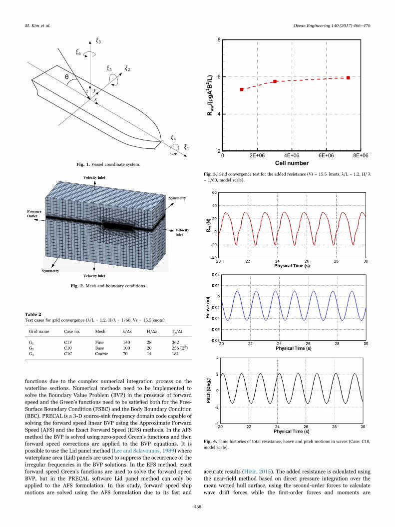
L x L−3 < < 1.25 , y L0 < < 2 , L z L−2 < < 1 where the mid-plane ofthe ship is located at y = 0 and ship draught (T) is at z=0. Theboundary conditions together with the generated meshes are depictedin Fig. 2. Artificial wave damping was applied to avoid the undesirableeffect of the reflected waves from the side and outlet boundaries.

4. Discussion of results

In this section, the simulation results using CFD and 3-D potentialmethods are presented and compared with available experimentaladded resistance (Lee et al., 2013) and ship motions data in regularhead waves. Unsteady wave patterns and time history results of theresistance and vertical ship motions in waves are simulated using aCFD method. Only two degrees of freedom motions, which are heaveand pitch responses, are calculated during all simulations.

4.1. Grid convergence test

Prior to the investigation of the added resistance and the heave andpitch motions using the CFD tool, grid convergence tests are performedto capture the accurate wavelength and height on the free surface. TheCFD simulations at 15.5 knots, which corresponds to the FroudeNumber (Fn) of 0.142, are carried out and the simulation results arecompared with the available experimental data. Grid convergence testsare performed at the wavelength to ship length ratio (λ/L) of 1.2 and atthe wave steepness (H/λ) 1/60. This wave condition corresponds to aresonant case (Sadat-Hosseini et al., 2013). The coarse and fine meshsystems are derived by reducing and increasing cell numbers perwavelength and cell height on free surface respectively using a factor of

2 (Bøckmann et al., 2014) as well as cell numbers on and around theship hull, which is affected by the mesh refinement on free surface,based on the base mesh case (Grid no G2, Case no. C10). Thesimulation time step is set to be proportional to the grid size as shownin Table 2.

where Te represents the corresponding encountering period.The results of the convergence tests with three different mesh

systems are shown in Fig. 3 where ρ, g and A denote the density,

Fig. 7. Snapshots of free surface elevation over one period of encounter (Case no. C10, Vs = 15.5 knots, λ/L = 1.2).

M. Kim et al. Ocean Engineering 140 (2017) 466–476

470

gravitational acceleration and the wave amplitude parameters respec-tively. As the number of cells increased, the added resistance coefficientincreased, especially from the coarse mesh (G3) to base mesh system(G2).

Additionally, in the current study, the grid uncertainty analysis isconducted using grid triplets G1, G2 and G3 with a uniform parameter

ratio (rG) chosen to be 2 for the free surface refinement. S1, S2 and S3are the corresponding solutions of the added resistance using the fine,base and coarse grids respectively and Rk is the convergence ratio asgiven in Eq. (8).

R εε

=kk

k

21

32 (8)

where ε S S= −K k k21 2 1 and ε S S= −K k k32 3 2 are the differences betweenbase-fine and coarse-base solutions and subscript k refers to the kthinput parameter which is G (i.e. grid-size) in this study. Griduncertainty study shows a monotonic convergence for the addedresistance with RG = 0.478 and the grid uncertainty with UG =3.759%S1 based on the Grid Convergence Index (GCI) method.Results reveals that the effects of the grid changes are small for thepresent range of grid size (Sadat-Hosseini et al., 2010). For moredetailed information on the calculation of the uncertainty analysis,reference can be made to Stern et al. (2006). Therefore the base meshsystem was chosen for the CFD simulations in this study while the cellnumber and time step vary according to the wave conditions in thesimulations.

Time (t/Te)

RW

(N)

0 0.25 0.5 0.75 1-40

-20

0

20

40

60

Time (t/Te)

Hea

ve(m

)

0 0.25 0.5 0.75 1-0.08

-0.04

0

0.04

Time (t/Te)

Pitc

h(D

eg.)

0 0.25 0.5 0.75 1-4

-2

0

2

4

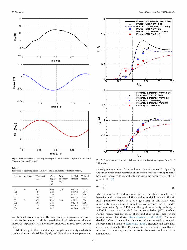
Fig. 8. Total resistance, heave and pitch response time histories at a period of encounter(Case no. C10, model scale).

Table 4Test cases at operating speed (12 knots) and at stationary conditions (0 knot).

Case no. Vs [knots] Wavelength(λ/L)

Waveheight(H)[m]

Wavesteepness(H/λ)

fe [Hz](model)

Te [sec.](model)

C71 12 0.75 4.00 1/60 0.9515 1.0510C72 1.00 5.33 0.7973 1.2542C73 1.20 6.40 0.7141 1.4004C73 1.40 7.47 0.6513 1.5355C81 0 0.75 4.00 1/60 0.7214 1.3862C82 1.00 5.33 0.6248 1.6006C83 1.20 6.40 0.5703 1.7534C84 1.40 7.47 0.5280 1.8939

Fig. 9. Comparison of heave and pitch responses at different ship speeds (V = 0, 12,15.5 knots).

M. Kim et al. Ocean Engineering 140 (2017) 466–476

471

In the 3-D potential flow method calculations, half of the ship's hullunder the still water level is modelled using around 1800 quadratic andtriangular panels while 8 panels per wavelength as the maximumlength of each panel are used for the highest encounter frequency.Regarding the computational time, for 3-D potential flow method thecomputational cost for each wave frequency, wave direction and shipspeed is about 20 s (single CPU at 2.7 GHz). The CFD method costsabout 1.5–2 days (36 CPUs at 2 GHz) for one wave condition, whichmeans that the 3-D potential method is much more cost efficient thanthe CFD for the calculations of the added resistance and ship motions.However, in 3-D potential method viscosity cannot be implemented inthe calculations due to the rigid-body linear method ship motions andadded resistance might be over-estimated around the resonant fre-quencies.

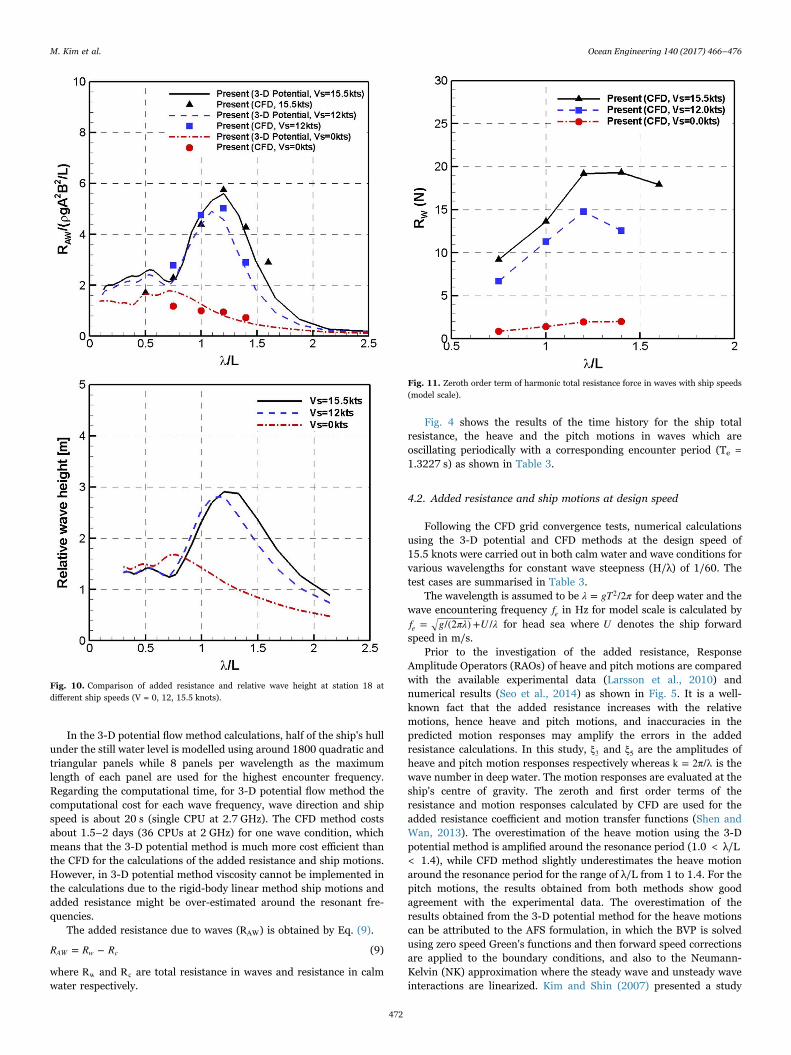
The added resistance due to waves (RAW) is obtained by Eq. (9).

R R R= −AW w c (9)

where Rw and Rc are total resistance in waves and resistance in calmwater respectively.

Fig. 4 shows the results of the time history for the ship totalresistance, the heave and the pitch motions in waves which areoscillating periodically with a corresponding encounter period (Te =1.3227 s) as shown in Table 3.

4.2. Added resistance and ship motions at design speed

Following the CFD grid convergence tests, numerical calculationsusing the 3-D potential and CFD methods at the design speed of15.5 knots were carried out in both calm water and wave conditions forvarious wavelengths for constant wave steepness (H/λ) of 1/60. Thetest cases are summarised in Table 3.

The wavelength is assumed to be λ gT π= /22 for deep water and thewave encountering frequency fe in Hz for model scale is calculated byf g πλ U λ= /(2 ) + /e for head sea where U denotes the ship forwardspeed in m/s.

Prior to the investigation of the added resistance, ResponseAmplitude Operators (RAOs) of heave and pitch motions are comparedwith the available experimental data (Larsson et al., 2010) andnumerical results (Seo et al., 2014) as shown in Fig. 5. It is a well-known fact that the added resistance increases with the relativemotions, hence heave and pitch motions, and inaccuracies in thepredicted motion responses may amplify the errors in the addedresistance calculations. In this study, ξ3 and ξ5 are the amplitudes ofheave and pitch motion responses respectively whereas k = 2π/λ is thewave number in deep water. The motion responses are evaluated at theship's centre of gravity. The zeroth and first order terms of theresistance and motion responses calculated by CFD are used for theadded resistance coefficient and motion transfer functions (Shen andWan, 2013). The overestimation of the heave motion using the 3-Dpotential method is amplified around the resonance period (1.0 < λ/L< 1.4), while CFD method slightly underestimates the heave motionaround the resonance period for the range of λ/L from 1 to 1.4. For thepitch motions, the results obtained from both methods show goodagreement with the experimental data. The overestimation of theresults obtained from the 3-D potential method for the heave motionscan be attributed to the AFS formulation, in which the BVP is solvedusing zero speed Green's functions and then forward speed correctionsare applied to the boundary conditions, and also to the Neumann-Kelvin (NK) approximation where the steady wave and unsteady waveinteractions are linearized. Kim and Shin (2007) presented a study

Fig. 10. Comparison of added resistance and relative wave height at station 18 atdifferent ship speeds (V = 0, 12, 15.5 knots).

Fig. 11. Zeroth order term of harmonic total resistance force in waves with ship speeds(model scale).

M. Kim et al. Ocean Engineering 140 (2017) 466–476

472

about the steady and unsteady flow interaction effects on advancingships and showed that in heave and pitch responses the NK approachoverestimates the heave and pitch responses compared to the experi-mental results, whereas the Double-Body (DB) and Steady Flowapproaches agreed well with the experiments. The underestimation ofthe results obtained from the CFD method is likely to stem from theadoption of a non-inertial reference frame in which large amplitudemotion causes inaccurate capturing of the free surface.

The numerical results of the added resistance are compared withthe available experiment data (Lee et al., 2013) and numerical results(Seo et al., 2014) as illustrated in Fig. 6, which indicates that the CFDand 3-D panel methods both have a reasonable agreement with theexperimental data except around the resonance period where bothmethods underestimate the added resistance. The authors will addressthis problem in future studies using a developed 3-D potential methodand adaptive mesh method in CFD simulations.

To visualise the ship motions and periodic wave patterns, the C10test case is selected in which the maximum added resistance isrecorded. Four snapshots of the waves and the vessel motions werecaptured with respect to the period of encounter at λ/L = 1.2 and at avessel speed of 15.5 knots. Results displayed in Fig. 7 show that thephenomenon of water on deck has been successfully captured by thecurrent CFDmodel. Fig. 7(c) is the snapshot at t/Te = 0.5 when the shiphas the largest resistance value as is shown in Fig. 8. In Fig. 7 thecontour on the hull and free surface indicates water height level takinginto account the ship vertical motions. Similarly to the snapshots inFig. 7, the time histories of total resistance force, heave and pitchmotions are displayed over an encounter period as shown in Fig. 8. Thelargest resistance force in waves is observed around t/Te = 0.5 when thebow is completely immersed and when the relative wave height is higharound the bow with green water on deck, as illustrated in Fig. 7(c).The position of the vessel where the maximum resistance is recorded iswhen the ship has the highest immersion due to heave motion, whilethe pitch amplitude is almost zero.

4.3. Added resistance and ship motions at stationary condition and atoperating speed

To consider the slow steaming or the realistic operating speeds ofthe vessel, the effect of ship speed on the added resistance and shipmotions was investigated (Tezdogan et al., 2015). In addition to theassumed operating speed (12 knots) as it was applied in SHOPERA(2016) Workshop, the cases for the stationary condition (0 knots) werealso simulated as summarised in Table 4. Wave conditions forwavelength and height are considered identical to those consideredin the simulations with the design speed cases.

Heave and pitch responses calculated by the CFD method arecompared with the results of the 3-D potential flow method for threeship speeds as shown in Fig. 9. It can be observed in Fig. 9 that 3-Dpotential flow method heave responses over-estimated the CFD resultsaround the resonant period. This can be explained by the steady and

unsteady flow interaction effects on advancing ships. Kim and Shin(2007) showed that in heave and pitch responses the NK approachoverestimates the heave and pitch responses compared to the experi-mental results, whereas they showed that NK approach provides moreaccurate added resistance estimations of blunt ships compared to theDB method. As it was mentioned before, in the present study, the 3-Dlinear potential flow method is applied to predict the ship motions andthe added resistance using the NK linearization scheme and near-fieldmethod in regular waves. It can be observed that at 12 knots and15.5 knots the heave and pitch response curves show the samepatterns. This can be explained by the AFS method because the BVPis solved at zero speed and forward speed corrections are applied to theforward speed cases. It is expected that at higher forward speed casesthe order of error will be higher than for the low forward speeds. Inzero speed simulations, heave and pitch response patterns are differentfrom the forward speed cases as expected.

The results for the mean added resistance in regular waves are alsocompared as shown in Fig. 10. The mean added resistance estimated bythe 3-D potential and CFD methods show good agreement and it isdemonstrated that the added resistance and ship motions can bepredicted reliably by using the current numerical approaches. Blok(1993) observed that in head seas the added resistance is increasingwith the increase in the ship speed, while the peaks of the addedresistance curves shift towards the longer wave periods. In the currentstudy, as it is shown in Fig. 10, Blok's observations are verified for theKVLCC2 and it is observed that the added resistance is augmented withthe increase in the ship speed around the resonance period (1.0 < λ/L< 1.4). However, in short waves the ship speed has minimal effect onthe added resistance because in short waves the added resistance ismainly affected by the governing diffraction forces near the bow.Another important phenomenon revealed in Fig. 10 is the closerelationship between the added resistance and the relative wave heightat Station 18 (130 m forward of midship) where it is observed that therelative motion is the main cause of the added resistance.

Zeroth order harmonic terms of the total resistance force are alsocompared using the CFD method for the stationary condition, shipoperating and design speeds as shown in Fig. 11. Total resistance inwaves increases with increasing ship speed as expected. This is due tothe increase in the calm water resistance and the augmented shipmotions, hence the increase in added resistance of the ship.

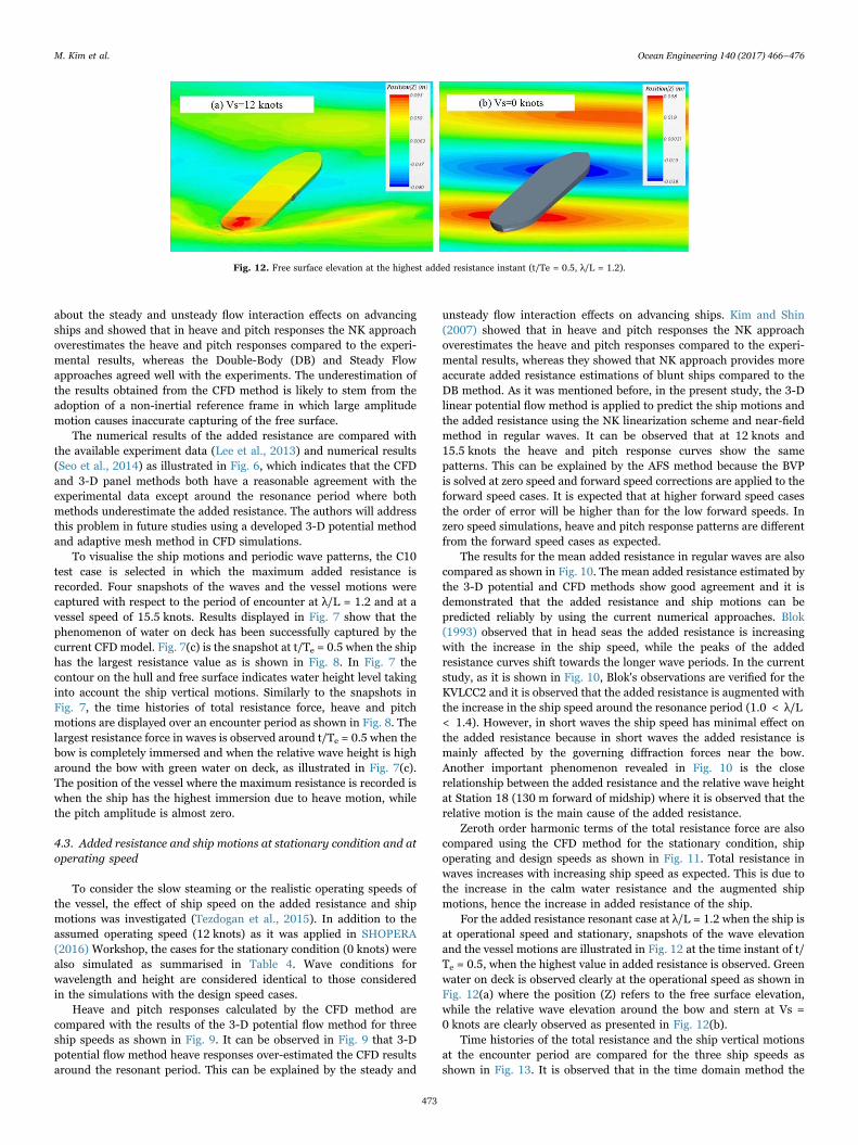
For the added resistance resonant case at λ/L = 1.2 when the ship isat operational speed and stationary, snapshots of the wave elevationand the vessel motions are illustrated in Fig. 12 at the time instant of t/Te = 0.5, when the highest value in added resistance is observed. Greenwater on deck is observed clearly at the operational speed as shown inFig. 12(a) where the position (Z) refers to the free surface elevation,while the relative wave elevation around the bow and stern at Vs =0 knots are clearly observed as presented in Fig. 12(b).

Time histories of the total resistance and the ship vertical motionsat the encounter period are compared for the three ship speeds asshown in Fig. 13. It is observed that in the time domain method the

Fig. 12. Free surface elevation at the highest added resistance instant (t/Te = 0.5, λ/L = 1.2).

M. Kim et al. Ocean Engineering 140 (2017) 466–476

473

oscillation amplitudes of the total resistance force in waves at thestationary condition are higher than at other speeds even though forthe stationary condition the mean total resistance in waves is muchlower than the other ship speeds, as shown in Fig. 11. It is shown inFig. 12 that unlike the forward speed simulations, at the stationarycondition there is no green water incidence observed. It should benoted that vessels in stationary condition should be carefully operatedin heavy weather conditions because the transient drift forces at zerospeed may be larger than the transient drift forces of a vessel advancingin waves. It is also noted that there are serious concerns regarding the

ship manoeuvrability at low speed in restricted areas in adverseweather conditions (Shigunov and Papanikolaou, 2015).

4.4. Added resistance and ship motions with varying wave steepness

The relationship between the added resistance and the ship verticalmotions for the wave steepness (H/λ) are investigated for a singlewavelength (λ/L = 1.2) at the design speed (Vs = 15.5 knots) assummarised in Table 5.

Time (t/Te)

RW

(N)

0 0.25 0.5 0.75 1-80

-40

0

40

80

120CFD (Vs=15.5kts)CFD (Vs=12kts)CFD (Vs=0kts)

Time (t/Te)

Hea

ve(m

)

0 0.25 0.5 0.75 1-0.06

-0.04

-0.02

0

0.02

0.04CFD (Vs=15.5kts)CFD (Vs=12kts)CFD (Vs=0kts)

Time (t/Te)

Pitc

h(D

eg.)

0 0.25 0.5 0.75 1-4

-2

0

2

4CFD (Vs=15.5kts)CFD (Vs=12kts)CFD (Vs=0kts)

Fig. 13. Total resistance, heave and pitch responses over one period of encounter (λ/L =1.2, model scale).

Table 5Test cases for wave steepness at Vs = 15.5 knots.

Case no. Wavelength(λ/L)

Wavesteepness (H/λ)

Waveheight (H)[m]

fe [Hz](model)

Te [sec.](model)

C20 1.2 1/150 2.56 1.3293 0.7523C30 1/100 3.84 1.0186 0.9818C40 1/80 4.80 0.8476 1.1798C10 1/60 6.40 0.7560 1.3227C50 1/50 7.68 0.6332 1.5793

H/λ

ξ 3/A

0 0.01 0.02 0.030

0.5

1

1.5

2Present (3-D Potential)Present (CFD)

H/λ

ξ 5/k

A

0 0.01 0.02 0.030

0.5

1

1.5Present (3-D Potential)Present (CFD)

Fig. 14. 1st order harmonic terms of non-dimensional heave and pitch responses fordifferent wave steepness (Vs = 15.5 knots, λ/L = 1.2).

M. Kim et al. Ocean Engineering 140 (2017) 466–476

474

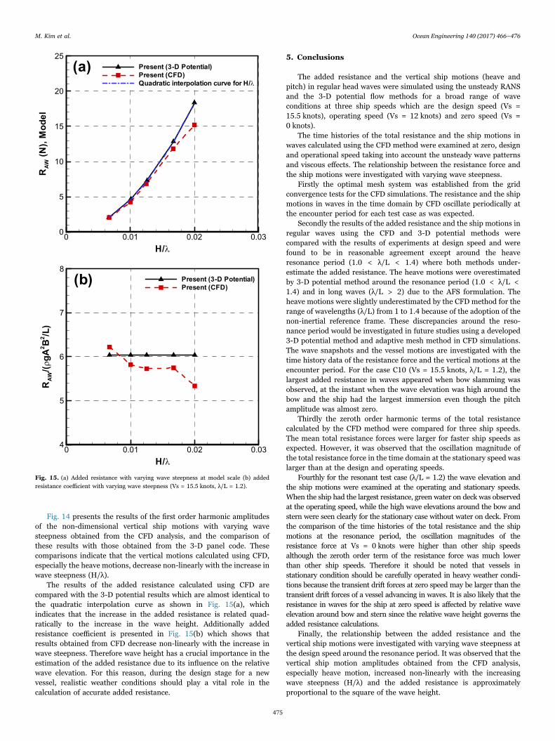
Fig. 14 presents the results of the first order harmonic amplitudesof the non-dimensional vertical ship motions with varying wavesteepness obtained from the CFD analysis, and the comparison ofthese results with those obtained from the 3-D panel code. Thesecomparisons indicate that the vertical motions calculated using CFD,especially the heave motions, decrease non-linearly with the increase inwave steepness (H/λ).

The results of the added resistance calculated using CFD arecompared with the 3-D potential results which are almost identical tothe quadratic interpolation curve as shown in Fig. 15(a), whichindicates that the increase in the added resistance is related quad-ratically to the increase in the wave height. Additionally addedresistance coefficient is presented in Fig. 15(b) which shows thatresults obtained from CFD decrease non-linearly with the increase inwave steepness. Therefore wave height has a crucial importance in theestimation of the added resistance due to its influence on the relativewave elevation. For this reason, during the design stage for a newvessel, realistic weather conditions should play a vital role in thecalculation of accurate added resistance.

5. Conclusions

The added resistance and the vertical ship motions (heave andpitch) in regular head waves were simulated using the unsteady RANSand the 3-D potential flow methods for a broad range of waveconditions at three ship speeds which are the design speed (Vs =15.5 knots), operating speed (Vs = 12 knots) and zero speed (Vs =0 knots).

The time histories of the total resistance and the ship motions inwaves calculated using the CFD method were examined at zero, designand operational speed taking into account the unsteady wave patternsand viscous effects. The relationship between the resistance force andthe ship motions were investigated with varying wave steepness.

Firstly the optimal mesh system was established from the gridconvergence tests for the CFD simulations. The resistance and the shipmotions in waves in the time domain by CFD oscillate periodically atthe encounter period for each test case as was expected.

Secondly the results of the added resistance and the ship motions inregular waves using the CFD and 3-D potential methods werecompared with the results of experiments at design speed and werefound to be in reasonable agreement except around the heaveresonance period (1.0 < λ/L < 1.4) where both methods under-estimate the added resistance. The heave motions were overestimatedby 3-D potential method around the resonance period (1.0 < λ/L <1.4) and in long waves (λ/L > 2) due to the AFS formulation. Theheave motions were slightly underestimated by the CFD method for therange of wavelengths (λ/L) from 1 to 1.4 because of the adoption of thenon-inertial reference frame. These discrepancies around the reso-nance period would be investigated in future studies using a developed3-D potential method and adaptive mesh method in CFD simulations.The wave snapshots and the vessel motions are investigated with thetime history data of the resistance force and the vertical motions at theencounter period. For the case C10 (Vs = 15.5 knots, λ/L = 1.2), thelargest added resistance in waves appeared when bow slamming wasobserved, at the instant when the wave elevation was high around thebow and the ship had the largest immersion even though the pitchamplitude was almost zero.

Thirdly the zeroth order harmonic terms of the total resistancecalculated by the CFD method were compared for three ship speeds.The mean total resistance forces were larger for faster ship speeds asexpected. However, it was observed that the oscillation magnitude ofthe total resistance force in the time domain at the stationary speed waslarger than at the design and operating speeds.

Fourthly for the resonant test case (λ/L = 1.2) the wave elevation andthe ship motions were examined at the operating and stationary speeds.When the ship had the largest resistance, green water on deck was observedat the operating speed, while the high wave elevations around the bow andstern were seen clearly for the stationary case without water on deck. Fromthe comparison of the time histories of the total resistance and the shipmotions at the resonance period, the oscillation magnitudes of theresistance force at Vs = 0 knots were higher than other ship speedsalthough the zeroth order term of the resistance force was much lowerthan other ship speeds. Therefore it should be noted that vessels instationary condition should be carefully operated in heavy weather condi-tions because the transient drift forces at zero speed may be larger than thetransient drift forces of a vessel advancing in waves. It is also likely that theresistance in waves for the ship at zero speed is affected by relative waveelevation around bow and stern since the relative wave height governs theadded resistance calculations.

Finally, the relationship between the added resistance and thevertical ship motions were investigated with varying wave steepness atthe design speed around the resonance period. It was observed that thevertical ship motion amplitudes obtained from the CFD analysis,especially heave motion, increased non-linearly with the increasingwave steepness (H/λ) and the added resistance is approximatelyproportional to the square of the wave height.

H/λ

RA

W(N

),M

odel

0 0.01 0.02 0.030

5

10

15

20

25Present (3-D Potential)Present (CFD)Quadratic interpolation curve for H/λ

(a)

H/λ

RA

W/(ρ

gA2 B

2 /L)

0 0.01 0.02 0.034

5

6

7

8Present (3-D Potential)Present (CFD)

(b)

Fig. 15. (a) Added resistance with varying wave steepness at model scale (b) addedresistance coefficient with varying wave steepness (Vs = 15.5 knots, λ/L = 1.2).

M. Kim et al. Ocean Engineering 140 (2017) 466–476

475

Acknowledgements

The authors are grateful to the Engineering and Physical ResearchCouncil (EPSRC) for funding the research reported in this paperthrough the project: “Shipping in Changing Climate”. (EPSRC grantno. EP/K039253/1).

The results given in the paper were obtained using the EPSRCfunded ARCHIE-WeSt High-Performance Computer (www.archie-west.ac.uk). EPSRC grant no. EP/K000586/1.

References

Arribas, F., 2007. Some methods to obtain the added resistance of a ship advancing inwaves. Ocean Eng. 34 (7), 946–955.

Blok, J.J., 1993. The Resistance Increase of a Ship in Waves. Delft University ofTechnology, TU Delft.

Bøckmann, A., Pâkozdi, C., Kristiansen, T., Jang, H., Kim, J., 2014. An experimental andcomputational development of a benchmark solution for the validation of numericalwave tanks. In: Proceedings of the 33rd International Conference on Ocean, Offshoreand Arctic Engineering. ASME.

Deng, G., Leroyer, A., Guilmineau, E., Queutey, P., Visonneau, M., Wackers, J., 2010.Verification and validation for unsteady computation. In: Proceedings of the Gothenburg2010: A Workshop on CFD in Ship Hydrodynamics. Gothenburg, Sweden.

El Moctar, B., Kaufmann, J., Ley, J., Oberhagemann, J., Shigunov, V., Zorn, T., 2010.Prediction of ship resistance and ship motions using RANSE. In: Proceedings of theWorkshop on Numerical Ship Hydrodynamics. Gothenburg, p. l.

Faltinsen, O.M., Minsaas, K.J., Liapis, N., Skjørdal, S.O., 1980. Prediction of resistanceand propulsion of a ship in a seaway. In: Proceedings of the 13th Symposium onNaval Hydrodynamics, Tokyo, pp. 505–529.

Gerritsma, J., Beukelman, W., 1972. Analysis of the resistance increase in waves of a fastcargo ship. Int. Shipbuild. Prog. 19 (217).

Gothenburg, 2010. A Workshop on Numerical Ship Hydrodynamics, Denmark.Guo, B., Steen, S., Deng, G., 2012. Seakeeping prediction of KVLCC2 in head waves with

RANS. Appl. Ocean Res. 35, 56–67.Havelock, T.H., 1937. The resistance of a ship among waves. Proc. R. Soc. Lond. Ser. A

Math. Phys. Sci., 299–308.Hizir, O.G., 2015. Three Dimensional Time Domain Simulation of Ship Motions and

Loads in Large Amplitude Waves. Naval Architecture, Ocean and MarineEngineering, University of Strathclyde, Glasgow.

IMO, 2012. Interim Guidelines for the Calculation of the Coefficient fw for Decrease inShip Speed in a Representative Sea Condition for Trial Use. International MaritimeOrganisation (IMO), London.

IMO, 2013. Interim Guidelines for Determining Minimum Propulsion Power to Maintainthe Manoeuvrability in Adverse Conditions. International Maritime Organisation(IMO), London.

ITTC, 2014. The Specialist Committee on Seakeeping-final Report andRecommendations to the 27th ITTC, International Towing Tank Conference,Copenhagen.

Joncquez, S.A., 2009. Second-Order Forces and Moments Acting on Ships in Waves.Technical University of Denmark, Copenhagen, Denmark.

Joosen, W.P.A., 1966. Added resistance of ships in waves. In: Proceedings of the 6thSymposium on Naval Hydrodynamics. National Academy Press, Washington D.C.

Kim, B., Shin, Y.S., 2007. Steady flow approximations in three-dimensional ship motioncalculation. J. Ship Res. 51 (3), 229–249.

Kim, H.T., Kim, J.J., Choi, N.Y., Lee, G.H., 2014. A study on the operating trim, shallowwater and wave effect. SNAK, 631–637.

Kim, K.H., Kim, Y., Kim, Y., 2007. WISH JIP Project Report and Manual. MarineHydrodynamic Laboratory, Seoul National University.

Kim, K.H., Seo, M.G., Kim, Y.H., 2012. Numerical analysis on added resistance of ships.Int. J. Offshore Polar Eng. 22 (01), 21–29.

Kim, M., Hizir, O., Turan, O., Day, S., Incecik, A., 2016. A study on ship speed loss due toadded resistance in a seaway. In: Proceedings of the 26th International Ocean andPolar Engineering Conference. Int. Soc. Offshore Polar Eng. Rhodes, Greece, pp.527–534.

Kim, M., Park, D.W., 2015. A study on the green ship design for ultra large containership. J. Korean Soc. Mar. Environ. Saf. 21 (5), 558–570.

Kim, Y.C., Kim, K.S., Kim, J., Kim, Y.S., Van, S.H., Jang, Y.H., 2015. Calculation of addedresistance in waves for KVLCC2 and its modified hull form using RANS-basedmethod. In: Proceedings of the 25th International Offshore and Polar EngineeringConference. Int. Soc. Offshore Polar Eng. Hawaii, USA, pp. 924–930.

Kwon, Y.J., 2008. Speed loss due to added resistance in wind and waves. Nav. Archit.,14–16.

Larsson, L., Stern, F., Visonneau, M., 2010. Proceedings Gothenburg 2010. In:Technology, C.U.o. (Ed.) A Workshop on Numerical Ship Hydrodynamics,Gothenburg, Sweden.

Lee, C.H., Sclavounos, P.D., 1989. Removing the irregular frequencies from integralequations in wave-body interactions. J. Fluid Mech. 207, 393–418.

Lee, J.H., Seo, M.G., Park, D.M., Yang, K.K., Kim, K.H., Kim, Y., 2013. Study on theeffects of hull form on added resistance. In: Proceedings of the 12th InternationalSymposium on Practical Design of Ships and Other Floating Structures. Changwon,Korea, pp. 329–337.

Liu, S., Papanikolaou, A., Zaraphonitis, G., 2011. Prediction of added resistance of shipsin waves. Ocean Eng. 38 (4), 641–650.

Mauro, H., 1960. The drift of a body floating on waves. J. Ship Res. 4, 1–5.Newman, J.N., 1967. The drift force and moment on ships in waves. J. Ship Res. 11 (1),

51–60.Park, D.M., Seo, M.G., Lee, J., Yang, K.Y., Kim, Y., 2014. Systematic experimental and

numerical analyses on added resistance in waves. J. Soc. Nav. Archit. Korea 51 (6),459–479.

Prpić-Oršić, J., Faltinsen, O.M., 2012. Estimation of ship speed loss and associated CO2emissions in a seaway. Ocean Eng. 44, 1–10.

Sadat-Hosseini, H., Carrica, P., Kim, H., Toda, Y., Stern, F., 2010. URANS simulation andvalidation of added resistance and motions of the KVLCC2 crude carrier with fixedand free surge conditions. Gothenburg 2010: A Workshop on CFD in ShipHydrodynamics.

Sadat-Hosseini, H., Wu, P., Carrica, P., Kim, H., Toda, Y., Stern, F., 2013. CFDverification and validation of added resistance and motions of KVLCC2 with fixedand free surge in short and long head waves. Ocean Eng. 59, 240–273.

Salvesen, N., Tuck, E.O., Faltinsen, O.M., 1970. Ship motions and sea loads. SNAME 104,119–137.

Seo, M.G., Yang, K.K., Park, D.M., Kim, Y., 2014. Numerical analysis of added resistanceon ships in short waves. Ocean Eng. 87, 97–110.

Shen, Z., Wan, D., 2013. RANS computations of added resistance and motions of a shipin head waves. Int. J. Offshore Polar Eng. 23 (04), 264–271.

Shigunov, V., Papanikolaou, A., 2015. Criteria for minimum powering andmaneuverability in adverse weather conditions. Ship Technol. Res. 62 (3), 140–147.

SHOPERA, 2016. Energy Efficient Safe Ship Operation EU FP-7 Project.SIMMAN, 2014. Workshop on Verification and Validation of Ship Manoeuvring

Simulation Methods. Denmark.Stern, F., Wilson, R., Shao, J., 2006. Quantitative V & V of CFD simulations and

certification of CFD codes. Int. J. Numer. Methods Fluids 50 (11), 1335–1355.Tezdogan, T., Demirel, Y.K., Kellett, P., Khorasanchi, M., Incecik, A., Turan, O., 2015.

Full-scale unsteady RANS CFD simulations of ship behaviour and performance inhead seas due to slow steaming. Ocean Eng. 97, 186–206.

Van't Veer, A.P., 2009. PRECAL v6.5 Theory Manual.

M. Kim et al. Ocean Engineering 140 (2017) 466–476

476