numerical studies in partial-differential equations of elliptic type
TRANSCRIPT

Glasgow Theses Service http://theses.gla.ac.uk/
Mathur, Suresh C. (1965) Numerical studies in partial differential equations of elliptic type. PhD thesis. http://theses.gla.ac.uk/3228/ Copyright and moral rights for this thesis are retained by the author A copy can be downloaded for personal non-commercial research or study, without prior permission or charge This thesis cannot be reproduced or quoted extensively from without first obtaining permission in writing from the Author The content must not be changed in any way or sold commercially in any format or medium without the formal permission of the Author When referring to this work, full bibliographic details including the author, title, awarding institution and date of the thesis must be given

NUMERICAL STUDIES IN PARTIAL DIFFERENTIAL
EQUATIONS OF ELLIPTIC TYPE being a Thesis presented
by SURESH CHANDRA MATHUR to the University of
Glasgow in application for the degree of DOCTOR OF
PHILOSOPHY.
September 1965
1 Of 119

`
Preface
The work presented in this thesis has been carried out under the supervision of Dr. D. C. Gilles.
The numerical results in Chapter V are to be published by Sneddon, Srivastav and Mathur.
I wish to offer my most sincere thanks to Dr. D. C. Gilles for his personal interest in me and for the encouragement and guidance I received from him.
I am also grateful to all members of the staff of the Computing Department for the willing cooperation they have shown me.
Suresh Chandra Mathur
2 Of 119

CONTENTS
Chapter 1 Treatment of curved boundaries in elliptic type partial differential equations, when
normal gradient is involved in boundary conditions.
Chapter 2 Mechnisation of the solution of Poissons’s equation
Chapter 3 Numerical treatment of reentrant corner in Laplace equation in cylindrical polars
with axial symmetry.
Chapter 4 Extension of Milne’s method to bi-harmonic equation.
Chapter 5 Numerical solution of two Fredholm type integral equations of second kind.
APPENDIX A
APPENDIX B
Index of reference
3 Of 119

INTRODUCTION
A variety of problems of physical interest are formulated in terms of elliptic partial differential equation. Well-known equations of this class are those of Laplace, Poisson and the bio-harmonic equation. The present work is the outcome of a study of some aspects of these equations. The problems included here are diverse in nature, and their study is numerical. Our aim is to explore numerical methods to handle each with adequate generality.
We devote a chapter to each problem. An outline of each chapter will now be presented.
In Chapter I we consider the case of curved boundaries in elliptic equations when the boundary conditions involve the normal gradient. Such boundaries have been considered by Fox (1950), Shaw (1950), Allen (1954), Viswanathan (1957), Varga (1957), Forsythe and Wasow (1959) and Greenspan (1965). Thus a variety of methods have been suggested for approximating the given partial differential equation at nodes, which lie adjacent to the curved boundary. In this chapter we present our approach towards this end. By including regional nodes as far as h√5 units from the typical node we developed relaxation patterns which have “almost” the same degree of accuracy as the formula for “irregular star”. Normally the resulting finite difference equations are diagonally dominant.
An ordering of nodes is suggested which reduces the band width of the coefficient matrix and also imparts Young’s property (A) to it.
Later, the technique is extended to treat boundaries of the “third type”, and an example considered by Allen, Fox, Southwell (1946) has been treated by it.
Chapter II presents the mechanization of the solution of Poisson’s equation. It is in partial answer to the big idea of developing a set of library programmes for the solution of similar equations, encountered so frequently in physical problems. A group of IBM 704 computer users, called SPADE, initiated this sort of project in 1957, and recently the KDF 9 Users group have worked up their own programme for the solution of Poisson’s equation. However these programmes cater only for a limited class of boundaries and layouts of the mesh over the region. On the other hand a general programme, which places no such restrictions, sounds a more welcome idea. Led by this thought we developed the programme we present here. The parametric difficulties with regard to the boundaries and the mesh have been overcome by combining appropriately with the user’s effort.
4 Of 119

Chapter III presents the numerical treatment of the re-entrant corner in Laplace’s equation in cylindrical polars with axial symmetry. Material of this nature seems to exists only with regard to the equations associated with the Laplaciam operator. The works of Motz (1946), Jeffreys and Jeffreys (1950), Woods (1953) and Wilson (1962) are noteworthy in this connection. Apparently, however, we adopt the same principles as employed by the above authors. Accordingly, an appropriate series solution to our equation is worked out to take account of the function near the singularity. Further the direct methods of Motz and Jeffreys and Jeffreys are modified to work them iteratively. This procedure eliminates the prohibitive amount of algebra involved in these methods.
To illustrate out approach, we set up an actual problem, and work it out fully.
Subsequently, we deal with the error analysis.
In Chapter IV we consider the eigen value problem associated with the biharmonic equation. Milne (1957) has suggested a method for the numerical evaluation of eigen values associated with the ordinary differential equations with two-dimensional Laplacian operator.
In this chapter the same method is extended to the biharmonic equation in two dimensions. It is shown that using this method it is possible to improve the eigen values considerably.
Chapter V presents the numerical solutions of two Fredholm integral equations of the second kind. They are taken from the analytical works of Sneddon (1962a) and Srivastav (1963). The evaluation of the kernel is particularly interesting in both of them. Analytical treatment is offered to remove the singularity. In addition, the kernel of the second integral equation is of special computational interest. The integrand involves subtracting two functions of almost the same magnitude. The loss of significant digits is, therefore, serious. The technique adopted here to cope with this situation is of general applicability.
Subsequently, the two solutions are checked using appropriate methods. They are shown to be satisfactory.
This completes a brief description of the material presented here. Lastly, we may emphasis that wherever necessary we have included appropriate examples to illustrate our approach.
5 Of 119

CHAPTER 1.
TREATMENT OF CURVED BOUNDARIES IN ELLIPTIC TYPE PARTIAL DIFFERENTIAL EQUATIONS, WHEN NORMAL GRADIENT IS
INVOLVED IN THE BOUNDARY CONDITIONS.
1.1 Introduction
The partial differential equations of the elliptic type are, in general associated with curved boundaries, and one of the most frequently used methods of solving them is the one which solves a related problem in finite differences. The given bounded region is covered with a suitable lattice of points, called the nodal points or the nodes. The nodes within the given region may be classified as:
(a)those lying on the given boundary or adjacent to it,(b)those lying within those of class (a).
At each node of class (b) the given partial differential equation is replaced by a suitable finite difference equation, while at nodes of class (a) the approximating finite difference equation incorporate the given boundary conditions in addition. The resulting system of finite difference equations is then solved simultaneously to give the wanted solution.
We thus notice that nodes of class (a) receive special treatment. In fact, no real difficulty is encountered in their treatment so long as the boundary cuts the lattice at nodal points only. But, equally so, the boundary may cut at non-nodal points as well. For example, a curved boundary may run across cutting the lattice at non-nodal points only. In such a situation, difficulty is experienced in developing reasonably accurate finite difference approximations to the given partial differential equation for (a) class nodes. It is the purpose of this chapter to present a general basis for developing suitable relaxation patterns for such difficult nodes, in problems in two dimensions.
With reference to figure 1, it is the point s like P and Q which have been referred to above as the difficult nodes. The point P
6 Of 119

Q
P
Figure 1.has just one interrupted arm, while Q has two. When more than two arms are affected the net needs to be replaced by a finer one, and such a case has not been considered here at all.
Whatever be the given partial differential equation, the handling of the difficult nodes depends largely upon the nature of the given boundary conditions. Accordingly, it seems worthwhile classifying the boundary conditions first. A general classification of the boundary conditions would be:
(1)When the wanted function is defined along the boundary;
(2)When the normal derivative of the wanted function is defined along the boundary;
(3)When the prescribed boundary condition is a linear combination of the above two conditions.
Condition (1) signifies simple Dirichlet boundary, and for such a boundary it is easy to derive relaxation patterns of reasonable accuracy. For example, for Nodes like P and Q, the formula for “Irregular star”, which is so commonly used in the solution of Poisson’s equation, is reasonably accurate – incorporating an error of the order of h for ∇ 2 u.
We do not propose to consider this kind of boundary here. What is intended, in fact, is to develop formulae of “almost” the same degree of accuracy for boundaries of the kinds (2) and (3).
Such boundaries have been considered by Shaw (1950), Fox (1950), Allen (1954), Viswanathan (1957), Varga (1957), Forsythe and Wasow (1959) and Greenspan (1965). The general treatment adopted by Fox, Shaw, Allen, Forsythe and Wasov, in such a situation, favors the inclusion of “fictitious points”. However, the problem with regard to the elimination of such “fictitious points” is, sometimes, found to be quite enormous, and often, it is hard to ascertain the order of accuracy of the
7 Of 119

resulting relaxation patterns. Viswanathan’s method, which is also based on finite difference theory, has the same order of accuracy as the formula for “irregular star” for Poisson’s equation. However, his relaxation pattern involved the radius of curvature of the boundary and also the first derivative of the given normal gradient with respect to the tangential direction at points where the boundary cuts the Lattice. The inclusion of these two parameters may, sometimes, discourage a programmer to use it freely in all sorts of boundaries. Varga’s method (Which is also described in Fox (1962)), though not based on finite difference theory is comparatively easy to program, but an account of its order of accuracy cannot be obtained in all kind of boundaries. However, the basis presented here develops formulae free from “ fictitious points”, and further, the order of their accuracy is clearly indicated. Greenspan’s approach is very much on the same lines as ours. A comparison would, therefore, be interesting. But we postpone it now, it is taken up exclusively in section 1.8; at the moment we proceed to present our approach.
1.2 The Present Approach
The basis of our approach is simple. What is suggested is that instead of including “fictitious points” in developing the relaxation patterns it is worthwhile including nodes from within the given region itself. It has been found that in most of the cases suitable regional nodes are never more than h√5 units away from the typical nodes. Even for a coarse mesh they can, therefore, be assumed to lie within the circle of convergence of the Taylor series of the wanted function about a typical node. Their inclusion does weaken the order of accuracy of the resulting relaxation pattern, but the price so paid is not so much as to disqualify them from consideration. For reasonably posed problems such nodes are easily available and the resulting relaxation pattern has ”almost” the same order of accuracy as the formulae for “irregular star” for Poisson’s equation.
To illustrate the approach, we will develop relaxation patterns for adjacent-to-the-boundary-nodes with boundary conditions of kinds (2) and (3).
1.3 Boundary Condition of Kind (2)
It is often referred to as the Neumann boundary and is commonly encountered in practice. We will illustrate our approach in relation to the solution of Poison’s equation in two independent variables x and y.
8 Of 119
Accordingly, the problem is to determine a function w inside a region R when a function g=g (x, y) is given within the said region such that
02
2
2
2
=+∂∂+
∂∂
gy
w
x
w(1)
and that
kv
w =∂∂
(2)
Being given on the boundary of R.
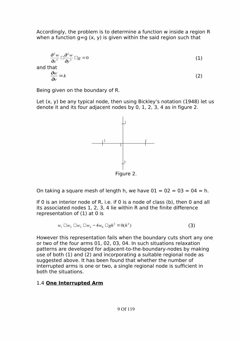
Let (x, y) be any typical node, then using Bickley’s notation (1948) let us denote it and its four adjacent nodes by 0, 1, 2, 3, 4 as in figure 2.
2
1
4
30
Figure 2.
On taking a square mesh of length h, we have 01 = 02 = 03 = 04 = h.
If 0 is an interior node of R, i.e. if 0 is a node of class (b), then 0 and all its associated nodes 1, 2, 3, 4 lie within R and the finite difference representation of (1) at 0 is
)(04 4204321 hghwwwww =+−+++ (3)
However this representation fails when the boundary cuts short any one or two of the four arms 01, 02, 03, 04. In such situations relaxation patterns are developed for adjacent-to-the-boundary-nodes by making use of both (1) and (2) and incorporating a suitable regional node as suggested above. It has been found that whether the number of interrupted arms is one or two, a single regional node is sufficient in both the situations.
1.4 One Interrupted Arm
9 Of 119

Considering the node 0, (fig.3) let use assume that only one of the arms, say 01, has been interrupted at N by the Neumann boundary.
2P x5
3h
0
4
h
h
h nN 1
+ α
υ
Figure 3.
Also, let 0N = h n nhN =0 where hhn ≤≤0 and let the normal at N make an angle ∝ with the interrupted arm in the positive sense. Then taking the node marked “5” as the regional node, suitable in this case, let us make our stand for a moment at P. Now assuming that the required function w has a Taylor Series at P and its circle of convergence encloses the points 2, 3, 4, 5 and N, we obtain
3
2
22
2
22
2 20
2
82
+
∂∂
+∂∂
∂+
∂∂
+
∂
∂
+
∂∂
+= h
y
w
yx
w
x
wh
y
w
x
whww pppppp (4)
3
2
22
2
22
3 20
2
82
+
∂∂
+∂∂
∂−
∂∂
+
∂
∂
∂
∂−= −
h
y
w
yx
w
x
wh
y
w
x
whww pppppp (5)
3
2
22
2
22
0 20
2
82
+
∂∂
+∂∂
∂+
∂∂
+
∂
∂
+
∂∂
+= h
y
w
yx
w
x
wh
y
w
x
whww pppppp (6)
3
2
22
2
22
4 2
30
96
8
3
2
+
∂∂
+∂∂
∂−
∂∂
+
∂∂
−
∂
∂+= h
y
w
yx
w
x
wh
y
w
x
whww pppppp (7)
3
2
22
2
22
5 2
30
69
8
3
2
+
∂∂
+∂∂
∂+
∂∂
+
∂
∂
+
∂∂−
+= h
y
w
yx
w
x
wh
y
w
x
whww pppppp (8)
Also at the point P we have from (1)
10 Of 119

02
2
2
2
=+∂
∂+
∂∂
gy
w
x
w pp (9)
Thus we have six equations in six unknowns.
2
22
2
2
,,,,y
wand
yx
w
x
w
y
w
x
ww pppppp ∂
∂∂∂
∂∂
∂∂
∂∂
∂ .
Hence on solving them we obtain
25432 2248 ghwwwwwp ++++=
220 2
12422 ghwwwx
wh p
p ++−=∂
∂
2
222
2
22
y
whgh
x
wh pp
∂∂
−−=∂
∂
42
52
23
22 24 wwwghw
yx
wh p
p −−−−=∂∂
∂ (10)
221
541
4321
02
22
4
322 ghwwwww
y
wh p
p −−+−−=∂
∂
Further the point N we have
2
20
22
++
∂∂
−∂
∂
++= n
ppnpN h
h
y
wh
x
wh
hww
Differentiating it w.r.t. x and y we obtain
2
2
2
20
2
22
++
∂∂∂
−∂
∂
++
∂∂
=∂
∂n
ppn
pN hh
yx
wh
x
wh
h
x
w
x
w
2
2
22
20
22
++
∂∂
−∂∂
∂
++
∂∂∂
=∂
∂n
ppn
pN hh
y
wh
yx
wh
h
yx
w
y
w
Multiplying both by 2h we have
++
∂∂∂
++
∂∂
=∂
∂ 22
220
2222 n
pn
pN hh
hyx
wh
hh
x
wh
x
wh
11 Of 119

++
∂∂
−∂∂
∂
++
∂∂
=∂
∂ 2
2
22
2
220
2222 n
ppn
pN hh
hy
wh
yx
wh
hh
y
wh
x
wh (11)
Now considering the boundary conditions (2) we write
v
wk N
∂∂
=1
v
y
y
w
v
x
x
w NN
∂∂
∂∂
+∂∂
∂∂
=
∝∂
∂+∝
∂∂
= Siny
wCos
x
w NN
or
y
whm
x
whSechk NN
∂∂
+∂
∂∝= 22,2 1 (12)
where ∝= tanmSubstituting the values of the derivatives from (11) we have form (12)
+∂∂
∂
−
++
∂∂
−∂
∂
++
∂∂
+∂
∂∝=
yx
whh
hmh
y
wmh
x
wh
hh
y
wmh
x
whSechk p
npp
npp
22
2
22
2
2
1 22
22222
+
2
220 nh
hh
On substituting the values of the knowns from (10) and simplifying, we obtain,
−
++−−
+++−
−−
−+−
+
24320
215
2112
2114
hgh
h
h
mhw
h
mhw
h
mh
h
hmw
h
mhwm
h
hw
h
h nnnnnnnn
( ) 302 23
1 hSechk ∝ =
denoting ξbyh
hn we can write it as
( ) ( ) ( ) ( ) −++−−+++−−−−−−+ 25430 )21(211222114 ghmwmwmmwmwmw ξξξξξξξξ
( ) 3
23
1 02 hSechk ∝ = (13)
It is the required relaxation pattern at 0.
12 Of 119

We observe that the finite-difference equation (13)
(a) is diagonally dominant,(b)is of non-negative type, (14)(c) imparts Young’s property A to the matrix
provided
m≥+ ξ21
1≤ξm (15)
It is apparent that (15) are fairly reasonable conditions and in most of the problems they should be easily satisfied.
So far we considered the case when m was positive. Now let us consider the case when m is negative. Figure 4 illustrates the nature of the boundary curve for a negative m.
υ5
3
2
0
4
N- α
Figure 4. In this case the suitable node is the marked “5” is the figure. The algebra involved here is almost the same as for positive m. Hence by a similar set of calculations we finally obtain difference equation at 0 to be
( ) ( ) ( ) ( ) ( ) −−+−+++−+−+−−+ 254320 2121122114 ghmwmwmwmwmw ξξξξξξξ
( ) 3
23
1 02 hSechk ∝ = (16)
We notice that equations (13 and (16) are the same, for if we set – m = n in (16) we obtain
( ) ( ) ( ) ( ) ( ) ( ) 3
23
12
54320 022121222114 hSechkghnnwwnwnwnw ∝ =−++−−−+−−−++−+ ξξξξξξ
13 Of 119

which is the same as (13) except that the coefficients of w2 and w4 have been exchanged.
Hence, we are now in a position to generalize our results.
If we denote
mP −+≡ ξ21
ξmQ 22 −≡
ξξ mmR +++≡ 21
Then according as the arms 01, 02, 03, or 04 is interrupted we have respectively at 0:
( ) ( ) 022114 12
54320 ∝=−++−−−−−+ SechkghmwmRwQwPww ξξξξ( ) ( ) 022114 1
251430 ∝=−++−−−−−+ SechkghmwmRwQwPww ξξξξ (17)
( ) ( ) 022114 12
52140 ∝=−++−−−−−+ SechkghmwmRwQwPww ξξξξ( ) ( ) 022114 1
253210 ∝=−++−−−−−+ SechkghmwmRwQwPww ξξξξ
While the conditions are
m≥+ ξ21
1≤ξm
When m is –ve, then R and P exchange positions.
When m = 0 the equations reduce to a form which does not require the regional node “5”. Also P = R then.
The following scheme indicates the position of the regional node in the different cases.
12 11
5 2 10
3 1
6
0
94
14 Of 119

7 8
The Interrupted arm Sign of m Nodes used in relaxation position
01 + 0, 2, 3, 4, 501 - 0, 2, 3, 4, 602 + 0, 3, 4, 1, 702 - 0, 3, 4, 1, 803 + 0, 4, 1, 2, 903 - 0, 4, 1, 2, 1004 + 0, 1, 2, 3, 1104 - 0, 1, 2, 3, 12
1.5 Two Interrupted Arms
The formulation of the relaxation patterns is simpler when the star has two interrupted arms. As pointed out earlier only one regional node is needed in this case as well. But the number of suitable nodes available here is two. We are, therefore, in a comfortable position. In a reasonable problem one of them should certainly lie within the region. However, when both lay inside the region the one which does not increase the band-width of the resulting finite difference matrix may well be selected.
Let the boundary cut the Lattice as in figure 5. Let 0N = ξ h, 0M = ηh
M
NO
3
4
6
5
Figure 5
15 Of 119

and the magnitude and direction of the normal gradient at N and M be
2211 , ∝∝ andkk respectively. Further let 2211 tan,tan ∝=∝= andmm , the
two regional nodes available here are marked “5” and “6” in the figure. The signs of m1 and m2 are of little consequence here. Moreover the algebra involved in the derivation has the same set of steps as we encountered earlier. Hence it would be better if we write down the required difference equation at 0 straight away. So, accordingly as the point marked “5” is the regional node, the finite difference equation at 0 is
05430 =−−−− edwcwbwaw (18)
where
( )212114 mmmnmna +−+++= ξξ ,
( ) ( ) ( ) ( )[ ]2121212 212212 mmnnmmmmnmb −−−−++−++= ξξξ ,
( ) ( ) ( ) ( )nmmmmnmmnmc +++−+−+++= ξξξ 22442 2121211 ,( ) ( )nmmmmnnmmd ++−+−= ξξξ 212121 2 ,
( ) ( ) ( ) ( )[ ] ( ) ( )[ ]2212121212 212122121211 ∝−++∝+++−+−+++++= SecmkSecmnkhmnmmnmghe n ξξξ
Next, if the point marked “6” is the regional node, the finite difference equation at 0 is still the same as equation (18), except that
w5 is replaced by w6
( ) ( ) ( ) ( )nmmmmnnmmmb +++−+−+−−= ξξξ 22442 2121212 ,
( ) ( ) ( ) ( )[ ]2121121 212212 mmnnmmmnmmc −−−+−+++= ξξξ
Other coefficients and the constant term remain the same.
It can be verified that in both the cases a, b, c, d should be positive for a reasonably posed problem. Hence equation (18) also enjoys the three properties enumerated in (14).
By an anticlockwise cyclic rotation of the suffixes of w in the second and third of (18) we can obtain finite difference approximations at 0 corresponding to stars with other pairs of interrupted arms.
16. An Example
16 Of 119

To illustrate the merits of the above formulae, we consider an example. For this sort of boundary Vishwanathan’s (1957) method is the most accurate of the existing methods. Hence to facilitate comparison with this method we solve the same problem which has been solved by him.
Hence we have to determine values of the harmonic function
( )2221 loglog yxrw +== inside the region ABCDE which is bounded by (figure
6).
x = 0 (straight line AE)
y = 2 (straight line ED)
x = 3 (straight line DC)
y = 0 (straight line CB)
14
22
=+ yx (Elliptic arc BA)
with v
w
∂∂
prescribed all along the border.
Here we have to solve Laplace’s equation, hence g = 0 in (1) and in the formulae developed above. By taking h = 0.25 we have covered the region with the same lattice of points as Vishwanathan.
17 Of 119

5
4 9
10
3 8
2 7
1 6
15
14
13
12
11
20
19
18
17
16
25
24
23
22
21
30
29
28
27
26
36
35
34
33
32
43
42
41
40
39
52
51
50
49
48
61
60
59
58
57
70
69
68
67
66
79
78
77
76
75
88
87
86
85
84P 1 P 2P 3 P 4
P 5
31 P 6 38 47 56 65 74 83
37 P 746 55 64 73 82
45 P 8 54 63 72 81
44 53 62 71 80
yE
A
D
xCB
Figure 6.
All the eight nodes adjacent to the elliptic boundary AB have interrupted arms. Of these P 6 and p 7 have two interrupted arms while the remaining six nodes have only one each. In order to use the difference equations established above we must first calculate ξ, η, k 1, k2, m1, m2
for both P6 and P7 and η, k, m for the rest. All this data is presented in Table I.
On the basis of this table the difference equations can be written down at once. They are in Table II.
At the boundary nodes A, B, C, D, E the finite difference equations can be obtained from (18) by setting ξ = η = m1 = m2 = 0 and substituting appropriate values of k1 and k2. The following table presents difference equations thus obtained at these nodes:
NODES
Finite Difference Equations
A 2 w 1 – w 6 – w
2 = -.250B 2 w 44 – w
53 – w 45 = -.125
C 2 w 80 – w 81 – w
71 = +. 083D 2 w 88 – w 79 – w 87 = +. 09615383E 2 w 5 – w 10 – w 4 = +. 125
18 Of 119
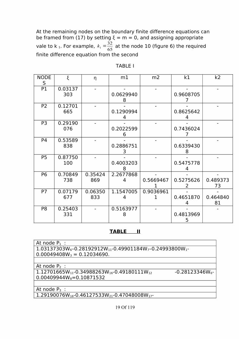
At the remaining nodes on the boundary finite difference equations can be framed from (17) by setting ξ = m = 0, and assigning appropriate
vale to k 1. For example, 65
321 =k at the node 10 (figure 6) the required
finite difference equation from the second
TABLE I
NODES
ξ η m1 m2 k1 k2
P1 0.03137303
- -0.0629940
8
- -0.9608705
7
-
P2 0.12701665
- -0.1290994
4
- -0.8625642
4
-
P3 0.29190076
- -0.2022599
6
- -0.7436024
7
-
P4 0.53589838
- -0.2886751
3
- -0.6339430
8
-
P5 0.87750100
- -0.4003203
8
- -0.5475778
4
-
P6 0.70849738
0.35424869
2.26778684
-0.5669467
1
-0.5275626
2
-0.489373
73P7 0.07179
6770.06350
8331.1547005
40.9036961
1-
0.46518704
-0.464840
81P8 0.25403
331- 0.5163977
8- -
0.48139695
-
TABLE II
At node P1 :1.03137303W6–0.28192912W11-0.49901184W7–0.24993800W1-0.00049408W3 = 0.12034690.
At node P2 :1.12701665W11-0.34988263W16-0.49180111W12 -0.28123346W6-0.00409944W8=0.10871532
At node P3 :1.29190076W16-0.46127533W21-0.47048008W17-
19 Of 119

0.34538539W11-.01475996W13=0.09483251.
At node P4 :1.53589838W21-0.62879311W26-0.42264973W22-0.44578041W16-.03867531W18=0.08247861.
At node P5 :1.87750100W26-0.87665098W32-0.32435923W27-0.58867040W21-.08782038W23=0.07372807.
At node P6 :0.24775907W31-0.13488774W38-0.05461757W32-0.05825376W27=0.02463398.
At node P7 :0.28752784W37-0.13888845W46-0.14305293W38-0.00558646W32=0.02370771.
At node P8 :1.25403331W45-0.24791721W44-0.43440888W54-0.53891166W46-.03279556W62=0.06772430.
of (17) is
65
1624 159510 −−−− wwww
It can be seen that the problem as formulated will not yield a unique solution. It will be general to the extend of an additive constant, which may be anything what-ever. Hence we have yet to impose an additional restriction to make it unique. We, therefore, use the fact that log r = 0 to A. Hence using w = 0 to A as another boundary condition we now solve the problem as a mixed boundary value problem. Now we need not consider an equation at A, rather we need to set w1 = 0 in the equations at the nodes P1 and “2”.
Having done this the results obtained are recorded in fig. 7. The true values and those of Vishwanathan are also given at each node for comparison.
1.6.1 Reducing the Band-width
It is true that due to the presence of the ‘extra nodes’ in our relaxation patterns, the band-width of the resulting matrix is, sometimes, much
20 Of 119

larger than it would otherwise be. However, the effect of such nodes on the size of the band-width can be eliminated by scanning the region diagonal-wise. The one diagonal, which is, in a sense, parallel to the curved boundary, would serve as the best
21 Of 119

56656975598
41641924102
24024282354
30303257
59559885889
45545814488
29529742888
11011161036
64064396340
51451705074
37537693674
22122312130
Vishwanathan's x 10 3
True x 10 4
present x 10 4
69870096909
58758935794
76376577556
66766916589
46947054604
56856975591
34534663356
46847054592
83283508247
90390628957
74975207415
83283508242
66666916581
76276577544
58658935773
69770096889
97497749667
91391639053
85485808466
80080477928
10441047510366
99199489836
94194549339
89690118891
11121115711046
10661070010587
10281027910162
98599059785
11781181611704
11381141811304
11011105510938
10691073710616
12981282512714
12061210211987
11241178611668
114611151311391
51351705029
64064396311
75475897465
85886368513
59459895861
71872357109
83083508224
95495949470
10421047510350
11231128911164
93193599233
10221027910152
11061112310995
69670096884
81281718044
91692139085
10101015710029
10961102110891
80681097983
91191639035
100610116
9987
10930984
10856
68969316808
55655965497
40240553986
22122312169
000
69770096903
68989316925
71972357130
75575897487
80180477946
85585808479
91391639061
97497749670
10361039710292
10981102
10913
11601163611528
12201223912129
12411245012838
Figure 7.
pointer. The band-width would, then, be a function of only the maximum number of nodes along any diagonal. Unless the diagonal is really too large, the band-width would be considerably reduced by this technique. Moreover such diagonal-wise scanning of the region would also impart a tri-diagonal representation to the resulting matrix, which, as Property (A), is found useful when the linear system is solved by successive over-relaxation.
In the example considered above the facts are as follows:
(1)If the nodes are taken in order, along the columns, that is, 1, 2, 3, 4, 5, 6, 7, 8,…;
(fig 6), the semi-band-width of the matrix is 17.
(2)If the nodes are taken in order, along the diagonals, that is 1; 6, 2; 11, 7, 3; 16, 12, 8, 4; 44, 21, 17, 13, 9, 5; 53, 45, 37, 31,… (fig. 6), the semi-band-width is 10.
22 Of 119

Thus a diagonal-wise ordering could reduce the semi-band-width from 17 to 10 in this case. It is a considerable achievement.
1.7. Boundaries of kind (3) There is no difficulty in extending this technique to problems with boundaries of the kind (3). It may happen that when the boundary conditions are ackward, a suitable regional node may not always be available to lend the sort of sophistication as achieved in the finite difference equations in the last sections. In such a situation, however, we can make good by achieving greater accuracy instead. A nearby node, distant h√ 2 would be a better choice than the one distant h√ 5 from the typical node.
As an example of this kind, we consider the problem of determining the stresses in an axially symmetrical solid of revolution when it is subjected to a given axial symmetrical pressure. This problem has been considered by Allen, Fox, Southwell (1946). Employing cylindrical polar coordinates, with z-axis as the solid of revolution, and as the stresses involved are independent of -, they have treated it as a two-dimensional problem in the z-r plane. The expressions for the four stress functions were derived by southwell (1942) in terms of two functions φ and ψ, both dependent on r and z only, such that over the plane region of rotation, the simultaneous governing equations are
01
2
2
2
2
=∂∂+
∂∂−
∂∂
zrrv
φφφ (19)
2
2
2
2
2
2 1
zzrrr ∂∂=
∂∂+
∂∂−
∂∂ φψψψ
(20)
While the conditions on the boundary are
( ) ( ) ( )zr
vz
rrrrvzrv
rrrvz
∂∂−
−
∂∂−=
−−
∂∂ ψψψφσφ ,cos1
,sin11
,sin22
(21)
( ) ( )r
vzzvrz
vz∂∂+=
∂∂ ψψ
,cos.,sin
(22)
zdsvr
.∫−=ψ + an arbitrary constant of integration (23)
Where ν is the direction of the outward drawn normal at a point on the boundary, and rv and zv are given stresses at that point in the r and z direction respectively. σ being Poisson’s ratio of the material of the solid of revolution.
23 Of 119
Hence the problem is to determine φ and ψ subject to governing equations (19), (20) and boundary conditions (21,22,23) over the plane region whose axial rotation generates the given solid.
As usual we cover the region with a square mesh of length h and examine interrupted stars adjacent to the boundary. Allen, Fox, Southwell (1946) have found the case harder when the star has an interrupted arm parallel to z-axis. The technique of introducing “fictitious points” which they have employed here does not proceed well when they try to eliminate them at a later stage. However in treating it with the technique presented here, no great difficulty is encountered. As the boundary conditions are really awkward here, the resulting finite difference equation is not quite sophisticated, but it promises better accuracy anyway.
We propose to work out the steps fully.
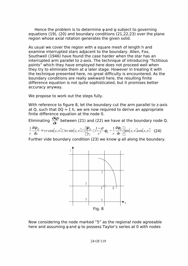
With reference to figure 8, let the boundary cut the arm parallel to z-axis at Q, such that 0Q = ξ h, we are now required to derive an appropriate finite difference equation at the node 0.
Eliminating r∂
∂ψ between (21) and (22) we have at the boundary node Q.
( ) ( ) ( ) ( )vzvzrrrr
vzzvvzrvzr
QQ ,cos,sin11
,sin,cos1
22
∂
∂−−+++=
∂∂ φ
φσψψ (24)
Further vide boundary condition (23) we know ψ all along the boundary.
r
2
3
5 4
0 Q
z
Fig. 8
Now considering the node marked “5” as the regional node agreeable here and assuming φ and ψ to possess Taylor’s series at 0 with nodes
24 Of 119

2,3,4,5,Q within its circle of convergence, we obtain for φ, retaining terms upto the second derivative only.
20
2220
0 2
1
zh
zhQ ∂
∂+
∂∂
+=φξφξφφ (25)
20
220
02 2
1
rh
rh
∂∂
+∂
∂+=
φφφφ (26)
20
220
03 2
1
zh
zh
∂∂
+∂
∂−=
φφφφ (27)
20
220
04 2
1
rh
rh
∂∂
+∂
∂−=
φφφφ (28)
20
20
2
20
2200
05 22
1
Rrzzh
rzh
∂∂
+
∂∂∂
+∂∂
+
∂∂
+∂
∂−=
φφφφφφφ (29)
Also, rewriting (19) at 0
01
2
200
20
2
=∂∂
+∂
∂−
∂∂
zrrr
φφφ (30)
Solving (25), (26), (27), (28) we have
04220
22 2φφφφ
−−=∂∂r
h (31)
( ) ( ) 0320
22 11
2
1 φξξφφφξξ +−+=∂
∂+ Qz
h (32)
( ) ( ) 42
320 11 φξφξφφξξ −−−=
∂∂
+ Qzh (33)
4202 φφφ
−=∂
∂r
h (34)
Substituting these values in (29) we get
( ) ( )[ ] ( ) ( )[ ] −+−++
−∂
∂+−−−
++−=
∂∂∂
030
02
32
050
22 1
1
11
1
1 φξξφφξξ
φφξφξφξξ
φφφQQ v
hrz
h
( )042 22
1 φφφ −+ (35)
again on substituting them in (31) we have
( ) ( ) ( ) 34202
211
2
1
211
2
11 ξφφξξφξξφξφ −
++−
−+−+−
r
h
r
hQ
(36)Now differentiating (25) w. r. t ‘r’ we have
25 Of 119

rzh
rrQ
∂∂∂
+∂
∂=
∂∂
02
0 φξφφ
Substituting for rQ
∂∂φ
and rz∂∂
∂ 02φ
, it is
( ) ( ) ( )[ ] ( ) ( )[ ] −+−++
−∂
∂
++−−−
++−=
∂∂
QQQQ
rhrrrhrhrrφξφξφ
ξφξφξφξφ
ξφφξφ
11
111
1
113
00
23
205
( )042 22
φφφξ −+rh
(37)
Replacing φ by Ψ in (25) and differentiating w. r. t. z
20
20
zh
zzQ
∂∂
+∂
∂=
∂∂ ψξψφ
or
( ) ( )[ ] ( )[ ]0302
320 1
1
21
1
1 ψξξψψξ
ψξψξψξξ
ψ+−+
++−−−
+=
∂∂
QQzh (38)
Substituting from (35), (36), (37), (38) in (24) we get
( ) ( ) ( ) ( ) ( ) ( ) ( ) +−+
−
++
+
+−++ vzvzrrrr
vzr
hvzzvhvzrvh Q ,cos,sin
1
1
1
21,sin,sin.,cos. 030
2
φξψξ
ξξξψ
ξξξψ
( )( ) ( ) ( ) ( ) ( ) ( ) ( ) −
+
−+−−
−+− vzvz
rr
h
r
hvzvz
rr
h,cos,sin
2
1
211
2
1,cos,sin11 220
2
2φξξσξξξσ
( ) ( ) ( ) ( ) ( ) ( ) ( ) −
−−−
+
−+−
vzvzrr
hvzvz
rr
h
r
h,cos,sin
1,cos,sin
2
1
211
2
132
22
φξξσφξξσ
( ) ( ) ( ) ( ) 0,cos,sin2
1
211
2
142
=
−−
−+−
vzvzrrr
h
r
h φξξξσ (39)
Now adding (19) and (20) and replacing the derivatives by difference coefficients we get for the node 0,
( ) 022
12
12
1
1
2
21
21
2
11
1 0423
440 =
−
++
−+
+
+
++
−+
+−
+φφφ
ξψψψ
ξξψ
ξξψ
r
h
r
h
rr
h
r
h
rrrQ
(40)
Adding (39) and (40 we finally get
26 Of 119

( ) ( ) ( ) ( ) ( ) ( ) ++−
+
++
−+
+
−++ 342
2 1
1
21
221
21
2,cos,sin,sin..,cos.. ξ
ξξψψ
ξψ
rr
h
rr
h
rrvzvz
r
hvzzvhvzrvh Q
( )( ) ( ) ( ) −
−
−+−r
vzvzrr
h 1,cos,sin
112
2
0
ξξσφ
( ) ( ) ( ) ( ) −
−−
+
−+−
r
h
rvzvz
rr
h
r
h
21
2
1,cos,sin
2
1
211
2
122 ξξσφ
( ) ( ) ( ) −
−−
vzvzrr
h,cos,sin
123
ξξσφ
( ) ( ) ( ) ( ) −
+−
−−
++−
r
h
rvzvz
rrr
h
r
h
21
2
1,cos,sin
2
1
211
2
124
ξξξσφ
( ) ( ) 0,cos,sin5 =vzvzr
ξφ
It is the required finite difference equation at the node 0.
This equation reduces to the one employed by Allen, Fox, Southwell (1946) for the rectangular region of rotation which they have considered in their numerical example.
1.8 Concluding Remarks
We will conclude this chapter by considering Greenspan’s work on this subject, which is by far the latest in the field, and as his line of approach is very much similar to ours, things are all the more interesting.In developing relaxation patterns for nodes adjacent to the Neumann boundary he also introduces extra nodes from within the given region.We will consider his method M2, which is more accurate. In Fig.9, if 0 be the node in question whose arms 01 and 02 have been interrupted by the Neumann boundary AB,
27 Of 119

3
5
0
4
B
A 30
4
B
A 1
2
6
5
Figure 9 Figure 10
Then the extra node included by him is the one marked ‘5’. Instead in our case, we include either ‘5’ or ‘6’ (Fig. 10)
Naturally his relaxation pattern should be more accurate than ours, but at the same time there are certain other points which also deserve notice. As greenspan points out his relaxation pattern lacks properties (14) and further, the algebraic system generated by it may have either no solution at all, or may have more than one solution. None of these things is present in our relaxation pattern.There is one more significant point in this connection. He dose not actually develop the relaxation pattern. For example, for the node 0, (fig. 9), he would like to incorporate as many as 3 equations in the linear algebraic system.
(a)For 0 using the formula for “irregular star”, imagining for a moment, that AB is a Dirichlet boundary.
(b)For A, expressing the normal derivative at A in terms of the function values at B, 0,4 and 5
(c) For B, this time expressing the normal derivative at B in terms of function values at A, 0, 3, 4 and 5.
Effectively this means that the number of linear algebraic equations in the resulting system would, in his case, be always greater than the number of nodes inside the given region. However this could have been easily avoided by straightway developing the relaxation pattern.From the above three equations after eliminating the function values at A and B.


CHAPTER II
MECHANISATION OF THE SOLUTION OF POISSON’S EQUATION
2.1 Introduction
Poisson’s equation is so frequently encountered in physical problems that the need to having a set of Horary programmes to mechanise the whole process of its solution is gaining wider recognition. As early as 1957, a group of IBM 704 computer users, called SPADE, initiated this sort of project with the idea of mechanizing the solution of both the elliptic and parabolic partial differential equations. A comprehensive account of how “ a very ambitious group of machine programmes was planned, and has been partially prepared” by them is given by Forsythe and Wasow (1960). The possibility of constructing a library of this sort of programme seems interesting to Fox (1962). The KDF 9 users group has gone far ahead. They have actually worked out a programme for the solution of Poisson’s equation (1964).
In broad outlines, the programme of both the SPADE and the KDF 9. Users group seems to have much in common. It is in the sense that
(a)both generate the mesh automatically
(b)both use interative methods for the solution of the system of algebraic equations.
They differ principally in their programming languages. While the SPADE programmes have been written in FORTRAN, the programme of the KDF 9 users group has been written in the KDF 9 user’s code
The idea of allowing the machine to generate the mesh is indeed quite helpful to the user, for what is then expected from him, as input data, is just a few parameters, which indicate the way the mesh is desired to be laid over the region. The subsequent task, starting from the evaluation of details for each node, to the final output stage, is then the care of the programme itself. This sort of mechanization which takes in least input data, and consequently expects least effort from the user, appears brilliant indeed. However, it must be remembered at the same time that this achievement has been made only at the expense of restricting the nature of the boundary associated with the given region. The SPADE programme allow the boundary to be arcs of conic sections or segments of straight

lines only; while the programme of the KDF 9 users group does not allow the boundary to be other than straight lines or circular arcs. In addition to these major restrictions there are a few minor ones as well. For instance one such restriction which the programme of the KDF 9 users group imposes is that no horizontal mesh line may cut the boundary in more than four points.
It is easy to see that, in view of these restrictions the scope of these programmes appears rather limited. A general programme which could allow the boundary to be any curve whatever, should therefore be a more welcome idea. Led by this thought we developed one such programme, and we propose to present it in this chapter. To be precise it is written in the KDF 9 ALGOL language (publication 1002).
This programme places no restrictions on the nature of the boundary or on the lay out of the mesh over the region. However this generality has been achieved only by asking the user to supply his own information with regard to the boundary and the conditions thereon. In doing so the user is not expected to have any previous experience in programming. Simple ALGOL statements are all that is required. There are five procedures to cover this, and they are described in details in section 2.2.1
In order not to involve the user any further in programming, we have avoided the idea of generating the mesh through the machine. The user is therefore expected to cover the region with a mesh of his own choice and describe the type of each node in a coded form. The code consists of twenty integral numbers and they can cater for all the types of node permissible. Along with this code description of each node is associated a few more parameters. All these numbers together form the required data. It is all described in details in section 2.2.1
The five procedures and the data is, therefore, all that our programme required from the user. Thus by making a reasonable compromise with the user we have overcome the parametric difficulties which hold back the mechanization process from acquiring a generality.There is yet another point where our programme differs from the programmes mentioned above. It is with regard to the method of solution of the system of finite difference equations. The above programmes use iterative methods, but we have adopted a direct method instead. Iterative methods are indeed advantageous for solving very large sparse systems, but for problems of moderate size, direct methods are preferable. They yield reasonably accurate solutions in a finite number of steps, while iterative methods may often require a very large number of iterations to yield the same degree of accuracy.

The fact that our programme is written in ALGOL imparts it yet another form of generality. As the ALGOL language is being internationally standardized, it is always possible to modify the programme to use it on any machine having an ALGOL translator.
2.2.1 Outlines of the programme
Our programme assumes that the given region over which Poisson’s equation is being considered is regular and none of its boundary points has any type of singularity either.Further the programme assumes that the region is covered with a square mesh.The boundary may be segment of any curve, and the condition thereon may be either Dirichlet (Function value specified) or Neumann (Normal derivative specified).In case of Dirichlet boundary the finite difference equivalence to poisson’s equation
( )yxgy
u
x
u,
2
2
2
2
=∂∂+
∂∂
is provided by the formula
( ) ( ) ( ) ( ) ( )yxghhhh
uhhh
u
hhh
u
hhh
u
hhh
u,
112
2222
42310
244
4
133
3
422
2
311
1 =
+−
++
++
++
+
Where 43210 ,,,, uuuuu are the function values in the accepted sense and 432,1 ,, hhhh are interrupted arms. Of course h is the mesh length. In case of
a regular interior node we have hhhhh ==== 4321 ,
and the above formula reduces to well-known form, viz.
( )yghuuuuu ,4 204321 =−+++ .
The programme assumes that not more than two arms of any node in the region have been interrupted by the boundary. If however this is not the case, the region need be covered with a finer mesh. A check on this is necessary because otherwise the programme will step out giving a failure signal.

In case of Neumann boundary, the finite difference equations are produced according to the patterns described in Chapter I. We have no intention of reproducing them here. We will however point out that before using the programme the user may make sure that the “extra” nodes demanded by those relaxation patterns are actually available inside the region, otherwise the programme will step out of the failure exit. Again the programme assumes that a maximum of only two arms of any node in the region have been interrupted by the Neumann boundary, and further , these arms are never apposite arms of a star. For instance a node with its first and third arms interrupted is not acceptable. Likewise any node with its second and fourth arms interrupted is not accepted either.
2.2 The programme
The programme comprises of three parts
1. The band formation
2. The band trimming
3. The solving process
4. The output part
Henceforth, we will call them as parts I, II, III and IV respectively. We now proceed to describe the function of each part.
2.2.1Part I ( The band formation)
This is by far the most important part of the whole programme . By itself it does a variety of jobs, and at the same time, prepares necessary data for the following three parts . As the user is directly concerned with this part, and with no other part at all, we propose to describe it in some detail.
To begin with, the user is required to plant the axes of reference in the plane of the given region. This he may to arbitrarily , keeping in view his convenience for expressing the nodes and the boundaries in terms of simple analytical geometry. Next with reference to these axes, he is required to write five ALGOL procedures, which hold information regarding

the Poisson-term, the nature of the boundaries and the conditions thereon. The five procedures are :
i) POISSONii) DESCRTiii) DIRIiv) NEUMv) DERV
In effect the programme assumes that the user has the poisson’s equation written in the form
( )yxgyx
,2
2
2
2
=∂∂+
∂∂ φφ
(1)
and the way the programme sets up the finite difference equations is in the matrix notation
bAx = (2)
Where , A is the coefficient matrix, b the right hand side and x the wanted vector.
Accordingly, it is in the context of (1) that the user writes the procedure POISSON to define the Poisson-term g in his case. There are three formula parameters in this procedure, let us call them 321 , andfff . The first two parameters , viz. 21andff refer to the x and the y coordinates of the node in equation. The third viz. 3f stands for the value of the Poisson-term g at that node. Hence , in this procedure user makes a single ALGOL statement, saying
( )213 ,: ffgf =
The procedure DESCRT defines the boundaries in terms of two-dimentional analytical geometry. There are five formal parameters in it. Let us call them
54,321 ,, andfffff .The first three viz. 3,2,1 andfff are called by value, while 5,4 andff are called by name . 1f and 2f stand for the x and y coordinates of the adjacent-to-the-boundary-nodes and 3f denotes the serial number of the boundary involved ( the boundaries are arbitrarily numbered by the user ). 54andff stand for the x and y coordinates of the points in which the boundary cuts the lattice.

B
P
A
Fig. 1
For example in fig. 1, Let the boundary AB cut the lattice in the points A and B, then 54andff stand for the x and y coordinates of A and B. Provided the equation to the boundary AB is given, it is possible to express 54andff
in terms of the coordinates 21andff of the node p. Thus, if the equation to AB is
32 =+ yx
then we can write
( )32
124 +−= ff
and 32 15 +−= ff
This information is sufficient to determine the coordinates of A and B; for, they are now
( ) ( )5124 ,, ffandff
respectively.
Although the programme uses this procedure to determine the coordinates of the points like A and B, the user is required only to express 54andff f4 in terms of 21andff . Thus ALGOL statements of the following form are written in this procedure :
if 13 bf = then begin ( ) ;2/3: 24 +−= ff
;32: 15 +−= xff
end;
where 1b is the serial number of the boundary involved here.
The next procedure is DIRI. It is meant to provide the function value on all the Dirichlet boundaries of the region. As told already the boundaries are arbitrarily numbered by the user and on each one of them the function values are described in simple ALGOL statements. There are four formal parameters in it. Let us call them 4321 ,, andffff . The first three parameters, viz. 321 , andfff are called by value, while 4f is called by the name. 21andff refer to the x and y coordinates of the points where the boundary cuts the lattice, and 3f is the serial number assigned to this boundary. 4f is of the type real and stands for the function value. Hence in this procedure the user makes statements, saying
if 13 bf = then 14 : Ff = ;if 23 bf = then 24 : Ff = ;
And so on. Here bn is the serial number of the boundary and nF is the function value on it.
The procedure NEUM is the analogue of the procedure DIRI. It defines the value of the normal derivative at each of the Neumann boundaries of the given region. Again there are 4 formal parameters in it ; let us call them
4321 ,, andffff . the first three parameters, viz. 321 , andfff have exactly the same references as in the procedure DIRI, and therefore , they hardly need to be explained any more. However , 4f stands for the normal gradient this time. But the ALGOL statements in this procedure , are given similar to the ones in the procedure DIRI. For example , we say
if 13 bf = then 14 : Nf = ;if 23 bf = then 24 : Nf = ;
etc. ,
Where nb denotes the serial number of the boundary and nN denotes the normal gradient on it.The least procedure is DERV. It provides the angles which the tangents to the boundaries make with the axis of x, measured in the positive sense. Hence , it describes the value of the angle.
( )dxdy /arctan

At each boundary on which the normal gradient is prescribed. Again, there are four formal parameters in it, and the first three have exactly the same meaning as in DIRI or in NEUM. 4f stands for the angle this time. The ALGOL statements are now
if 13 bf = then 14 : Af = ;if 23 bf = then 24 : Af = ;
Where nb denotes the serial number of the boundary involved here, and nA denotes the angle which the tangent to the boundary makes with x-axis
in the positive sense. It is clear that, depending upon the nature of the boundary, the expression for An will involve the parameters 21andff .
In addition to the five procedures mentioned above , the user is also required to furnish a small piece of data. Essentially , it is a row-wise (or column-wise) description of the types of the nodes he has in the region.
An assortment of twenty types of nodes is permissible. It is divided into four categories :
(i) 0 ;
(ii) 1 ;
(iii) –1, -2, -3, -4, -12, -13, -14, -23, -24, -34 ;
(iv) –11, -22, -33, -44, -1122, -2233, -3344, -1144.
We now proceed to describe each category.
An O-type node is a node on a Dirichlet boundary. No difference equation corresponding to this node is set up.
A 1-type node is an interior node. It has no interrupted arm, all its four neighboring nodes exist the region.
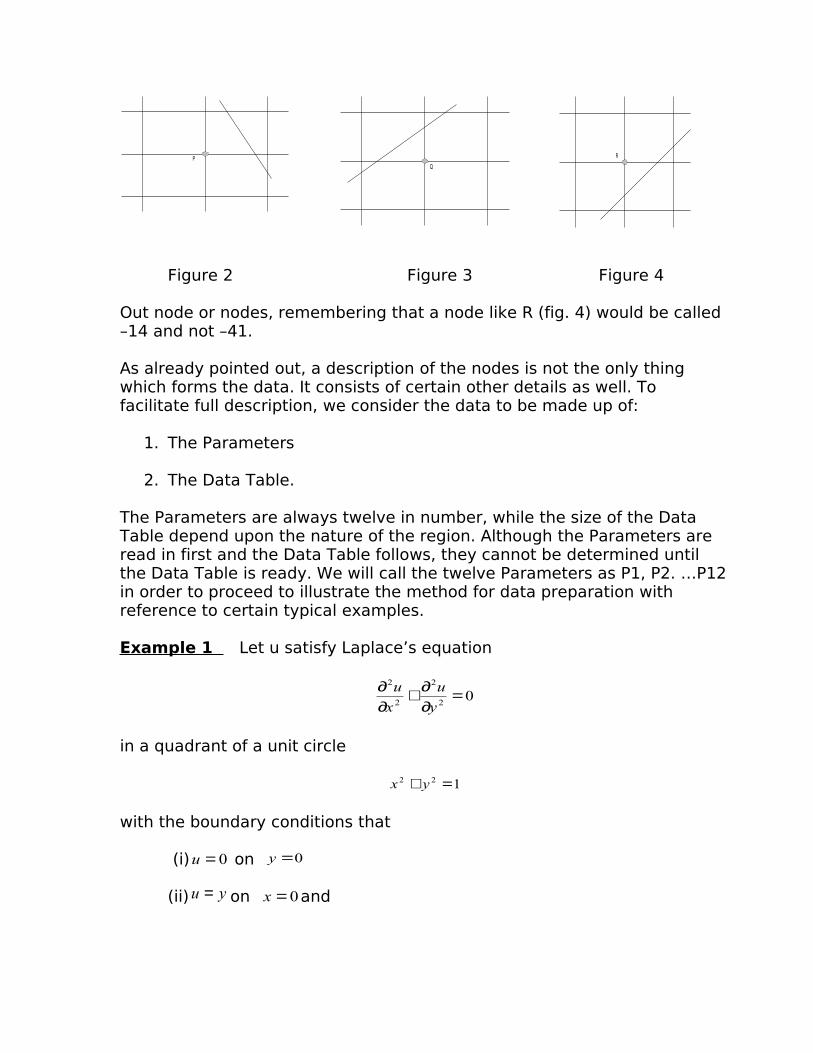
The category (iii) refers to nodes with arms interrupted by one or two Dirichlet boundaries. For example, the node P (fig. 2) will be of the type –1, and Q (fig. 3) of the type –23. The idea is to call the missed
PQ
R
Figure 2 Figure 3 Figure 4
Out node or nodes, remembering that a node like R (fig. 4) would be called –14 and not –41.
As already pointed out, a description of the nodes is not the only thing which forms the data. It consists of certain other details as well. To facilitate full description, we consider the data to be made up of:
1. The Parameters
2. The Data Table.
The Parameters are always twelve in number, while the size of the Data Table depend upon the nature of the region. Although the Parameters are read in first and the Data Table follows, they cannot be determined until the Data Table is ready. We will call the twelve Parameters as P1, P2. …P12 in order to proceed to illustrate the method for data preparation with reference to certain typical examples.
Example 1 Let u satisfy Laplace’s equation
02
2
2
2
=∂∂+
∂∂
y
u
x
u
in a quadrant of a unit circle
122 =+ yx
with the boundary conditions that
(i) 0=u on 0=y
(ii) yu = on 0=x and
(iii) yy
u =∂∂
∂u/∂y on the circular arc. To findu .
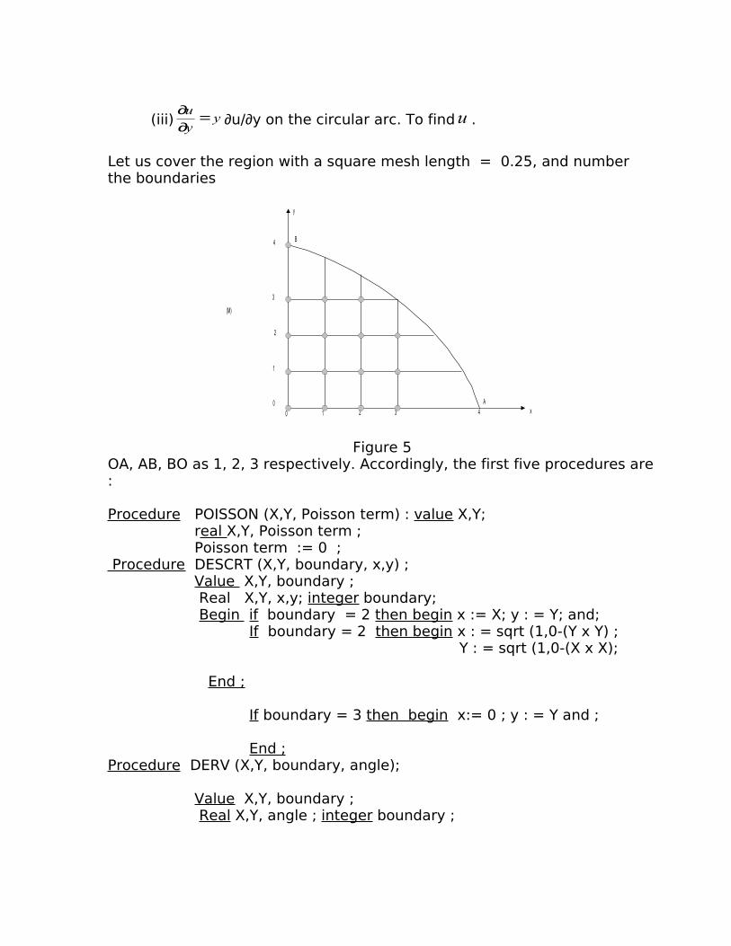
Let us cover the region with a square mesh length = 0.25, and number the boundaries
y
B
Ax0 1 2 3 4
(M)
4
3
2
1
0
Figure 5OA, AB, BO as 1, 2, 3 respectively. Accordingly, the first five procedures are :
Procedure POISSON (X,Y, Poisson term) : value X,Y; real X,Y, Poisson term ; Poisson term := 0 ; Procedure DESCRT (X,Y, boundary, x,y) ; Value X,Y, boundary ; Real X,Y, x,y; integer boundary; Begin if boundary = 2 then begin x := X; y : = Y; and; If boundary = 2 then begin x : = sqrt (1,0-(Y x Y) ; Y : = sqrt (1,0-(X x X);
End ;
If boundary = 3 then begin x:= 0 ; y : = Y and ;
End ;Procedure DERV (X,Y, boundary, angle);
Value X,Y, boundary ; Real X,Y, angle ; integer boundary ;

Begin if boundary = 1 then angle : = 0; If boundary = 2 then angle : = 3.14159265-arctan (X/Y); If boundary = 3 then angle : = 1.57079633; End;
Procedure DIRI (X,Y, boundary,d); Value X,Y,boundary; Real X,Y,d; integer boundary ; Begin if boundary = 1 then d : = 0 ; If boundary = 3 then d : = y; End ;
Procedure NEUM (X,Y,boundary,n); Value X,Y, boundary ; Real X,Y, n; integer boundary;
Begin if boundary = 2 then n : = y; End ;
Now, having read in the procedures, we have yet to read in the data. As already pointed out , we will prepare the data table first and the parameters next, although they are fed into machine in the reverse order.
All the nodes marked with a thick dot are the Dirichlet boundary nodes and are , therefore , of the type 0. The remaining nodes , marked with crosses, are of the types specified in categories (ii), (iii) and (iv) above. All the nodes, irrespective of their category , are described in the Data Table. But the user has to decide the way he prefers their description. There are four ways of describing these nodes;
(a)row-wise, upwards, starting from the lowest;
(b)row-wise, downwards, starting from the uppermost ;
(c) column-wise, from left to right;
(d)column-wise , from right to left. Let us choose the way specified in, say, (A). The form of the Data Table for this problem is;

1; 14; 0;1; 0;4; 0;0;0;0;0; 1;1;1;1;1;
1; 9; 1;1; 0;3; 0;2;-11; 3;2;
1; 10; 2;1; 0;3; 0;2;-1122; 3;2;2; …..(m)
1; 11; 3;1; 0;2; 0;-22;-1122; 3;2;2;2;
1; 6; 4;1; 0;0; 0; 3;
We will now explain this table. It consists of five arrays, and they are allconstructed in the same fashion. A description of any one of them, will therefore, cover for the rest. Let us take up the middle array marked (M) and explain the meaning of each of its elements. This array refers to the row marked (M) in figure 5.
The first element is 1. This indicates that there is only one row of this nature. None of its adjacent rows is its copy.
The next element is 10. It is just the count of the elements which follow it in the array (M).
The third element is 2. It is the ordinate of this row. The unit of measurement being the mesh length. Obviously, if the row is towards y- increasing this integer is positive. If the row is on the –ve side of the –y axis, then this number is negative.
The fourth element is 1. It means that this row is just one continuous whole. If the given region is pierced with holes then the whole row would be broken up in to segments. The number occurring here is actually the count of these segments.
The fifth and the sixth elements refer to the abscissa of the first and the last nodes of this row in units of mesh lengths.
The following three elements indicate the types of the nodes in this row. The first node is of the type O. The next two nodes are of the type 1, and since, both the nodes are adjacently placed, we can economise by just writing 2, in place of 1; 1;. The fourth node has its first and the second arm interrupted by the Neumann boundary AB; accordingly, it is of the type –1122.

The last three elements describe the boundaries affecting the nodes of this row. The first node of this row lies on OB which is our boundary no. 3. Hence, 3 appear as the first of these three elements. The remaining two elements, viz. 2; 2; refer to the boundary no. 2, i.e. AB which has affected the two arms of the last node of this row. It may be emphasized here that whenever two arms are interrupted, both the boundaries need be declared.
This completes the description of the array (M) pertaining to the row (M) in figure. 5. The same applies to the rest of the rows of the above Data Table, and any more explanation is, therefore, unnecessary. We can now proceed ahead to the parametric part of the data. The 12 parameters written with the help of the above Data Table are as follows:
51 =P ; (Total no. of rows in the given region).
52 =P ; (No. of nodes in a row which has a maximum of them).
33 =P ; (No. of nodes, not of type O, in a row which has a maximum of them).
94 =P ; (total no. of nodes in the region which are of type O).
15 =P ; (As an indication of whether we are reading the region in the positive or the negative direction we use +1 or –1. Whenever we are reading row-wise upwards, or column-wise from left to right, 15 +=P . Alternatively, a row-wise downwards read, or a column-wise right to left read assigns 15 −=P ).
16 =P ; (When we read row-wise 16 =P , and when we read column-wise06 =P . Here we are reading row-wise, hence 16 =P ).
07 =P ; (A row-wise read means that 07 =P , while a column-wise read means that 17 =P . Here, we are reading in row-wise, hence 07 =P .
25.08 =P ; (It is the mesh length).
149 =P ; (It is the maximum number appearing in col.2 in Data Table).
510 =P ; (Total no. of arrays in the Data Table).
511 =P ; (The function values are output in exact geometric positions of the corresponding nodes. A maximum of eight columns is permissible. If the

number of columns, in the given region, exceeds eight, an automatic page change takes place. Hence the number mentioned in this position should never be greater than 8. in our problem we have only five columns, hence it is 5 here).
012 =P ; (Both the fixed and the floating form of outputs are possible. A “0” indicates a fixed format –n ddddd , while a “1” indicates floating format
nddddddd ≠− 10. ).
Thus we have furnished a full description of all the 12 parameters. With the procedures already given, the information, necessary for the solution of this problem is now complete. No further detail is required.
Before moving to the next example, we would like to point out certain subtle points with reference to the above example. When the nodes are read in row-wise, the width of the band is a function of the maximum number of non-0-type nodes in any one row. On the other hand, if we read in column-wise the band width is a function of the maximum number of non-0-type nods in any one column. In the particular example above the maximum number of nodes, row-wise and column-wise, is the same viz. 3. But in most of the problem they are different, and naturally and advantage is gained by choosing the one which is least. The shorter the bad the better it is. It is why, the user may sometimes, prefer to read in column-wise. As an illustration of how the data, for the above example could be read in column-wise, from right to left, we have the following form.
The Parameters
5; 5; 3; 9; -1; 0; 0.25; 14; 5; 5; 0
The Data Table
1; 6; 4; 1; 0;0; 0; 1;
1; 11; 3; 1; 0; 2; 0; -11; -1122; 1; 2; 2; 2;
1; 10; 2; 1; 0; 3; 0; 2; -1122 1; 2; 2; 2;
1; 9; 1; 1; 0; 3; 0; 2; -22; 1; 2;
1; 14; 0; 1; 0; 4; 0; 0; 0; 0; 0; 3; 3; 3; 3;

In the context of the explanation already given, it is easy to understand how the Parameters and the Data Table have been written out in the above form. The procedures hold good whatever way the data is read in.
Example 2 Let the stress-function u satisfy Poisson’s equation.
22
2
2
2
−=∂∂+
∂∂
y
u
x
u
Inside an H-section girder, (fig.6) u=0 on the boundary. Solve for u inside the region. But, in order to bring into focus certain aspects of the Programme, which could not be illustrated by Example 1, we propose to consider the whole of the H-shaped region ABCDEFGHJKLMN.
Having covered it up with a suitable net of mesh length h, let use
L M
N J
H G
x
y
A B
C D
E F
0
1
2
3
(N)
Figure 6.
Plant the axes of reference as shown in figure 6, and number the boundaries in the following order.
Name of the boundary Number allocate to itAB and EF 1
BC 2CD 3DE 4

FG 5GH AND LM 6
HJ 7JN 8NM 9LA 10
We now decide that we will read in row-wise, from ABEP to LMHG, i.e. towards y – increasing. Accordingly the Parameters and the Data Table are:
13; 13; 11; 62; 1; 1; 0; h; 26; 7; 8; 0;
1; 26; -6;2; -6;-2;2;6; 0;0;0;0;0;0;0;0;0;0; 1;1;1;1;1;1;1;1;1;1;
3; 16; -5;2; -6;-2;2;6; 0;3;0;0;3;0; 10;2;4;5; (N)
1; 20; -2;1; -6;6; 0;3;0;0;0;0;0;3;0; 10;3;3;3;3;3;5;
3; 9; -1;1; -6;6; 0;11;0; 10;5;
1; 20; 2;1; -6;6; 0;3;0;0;0;0;0;3;0; 10;8;8;8;8;8;5;
3; 16; 3;2; -6;-2;2;6; 0;3;0;0;3;0; 10;9;7;5;
1; 26; 6;2; -6;-2;2;6; 0;0;0;0;0;0;0;0;0;0; 10;10;10;10;10;10;10;10;10;10;
Here we need not explain the parameters. They are written in the manner already explained in example 1. We will only discuss the second array marked (N) in above table. This array corresponds to the three rows, collectively marked (N) in fig. 6.
The first element of this array is 3. It suggests to the machine that there are three adjacent rows (marked 1,2,3 in fig. 6) which have the same description. In such a situation, a description of the first one of them is given. Hence we will describe the one marked “1” here.
The second element is 16. It is the count of the elements which follow it in the array (N).The third element , which is –5 is the ordinate of the first row, in units of mesh length.

The fourth element is 2. It indicates that each of these rows has two segments.
The fifth and sixth elements are –6 and –2. They are the abscissa of the first and the last nodes of the first segment. The seventh and eighth elements, which are 2 and 6, are, similarly, the abscissa of the first and last nodes of the second segment. The unit of measurement being the mesh length.
The rest of the elements have nothing new to be explained about. They bear the same explanation as in Example 1.We thus notice that instead of writing 3 arrays for the 3 rows, we have economized by just writing the details of only the first of them. Another things worth noticing is the way the different segments of a row have been described.
2.2.2Part II (the band trimming)
The band formed by part I is written down on a magnetic tape. It may well be, that the band so formed may have quite a few columns of zero elements on both sides of it. Such zero-columns should simultaneously be dropped from both the sides, because, while it does not affect the analysis, it does help a great deal by way of reducing the band width.Accordingly, the part of the programme inspected the band as formed by part I, and, if necessary, trims it form both the sides. The finished band, as produced by this part, has the minimum band width possible.The crude version of the band is, then, over-written by finished one.The user has nothing to do with this part directly, because, as soon as part I is over, this part steps in automatically.
2.2.3Part III (the solving process)
The finished version of the band equation, as produced by part II, is then solved against the right hand side produced by part I. This solution over-writes the band this time.The simple elimination method without interchanges is the one used here in the solution of the band equations. The given band A is factorised into lower and upper triangular bands I and U such that A = LU.
The factorization is always possible so long as none of the leading minors of the matrix is zero. The solution of the linear equations is then straightforward for, if we write them as
Ax = b
Then using A = LU
We have Lux = b
If we denote Ux by the vector y, then we obtain two sets of equations viz.,
Ly = b
And Ux = yThe former is solved for y by forward substitution, while the latter on subsequent back-substitution yields the required solution x.The finite difference equations set up by part I are diagonally dominate are of the non-negative type. Further, all the equations are so normalized that the diagonal-coefficients in A are all unity.The factors I, and U over –write A in the core store. This is always possible, since they conform to the band structure of A.The programme assumes that A is non-symmetric. Hence, in problems which produce symmetric matrices, no advantage can be gained either in storage space or in time.
2.2.4. Part IV (the output part)
This part outputs the solution produced by part III in a presentable form.The region described by the user in part I is now reproduced geometrically and at the nodes are written the function values. Whether the data has been read in row-wise or column-wise at the part I stage, the output here is always row-wise, which is actually the desirable form.
The two formats used to output the solution have already been explained in section 2.2.1. Further, it is not possible to output more than eight columns of the region at a time. If, however, the region has more than eight columns, as automatic page change takes place.
Stream 70 has been used for output, which allows the user the facility of obtaining the output on any device of his choice.
2.3 The working of the programme

The input is via the paper tape. The 5 procedure go after the title of the programme. The date waits till it is called. The output is through any device of the users choice.
For storing the intermediate dates, the programme requires two magnetic tapes bearing the identifiers :
21φφφφDG and 31φφφφDG
Part I and IV use both the magnetic tapes, while the parts II and III use the one labeled 21φφφφDG only.
Part I writes on the two magnetic tapes in the following manner: on 21φφφφDG are written out the band matrix and the right hand side. On 31φφφφDG are written out 3 blocks of information. The first two blocks
contain information subsequently necessary for arranging the output, while the third block is a vector containing . Function values at nodes on the Dirichlet boundary. As a matter of fact, this vector is also stored for use at the output time only.
As soon as part I has completed its work, part II takes over automatically. As described already , this part time the band (if necessary) and the trimmed version over-writes what was there on 21φφφφDG so far.
Next the control is automatically passed on to part III, which brings the band and the right hand side into the high speed store and does the solution to the problem. The results are written back on 21φφφφDG . .
Finally , part IV steps up, and in accordance with the information on tape 31φφφφDG outputs the results in the required format.
As the programme is progressing , from one stage to the other , indications are sent out to the user via the monitor typewriter. Thus he is able to follow the programme step by step.
We would like to conclude by emphasizing that in elliptic equations the demand is always on the store. Hence we have tried to shape the programme so that a maximum storage is left available to hold the data. The time factor is, therefore , often overlooked.
The flow chart of part I and the programme failures are appended in A(2) I and A(2)II respectively.

CHAPTER III
NUMERICAL TREATMENT OF RE-ENTRANT CORNER IN LAPLACEEQUATION IN CYLENDRICAL POLARS WITH AXIAL SYMMETRY
3.1 Introduction
A variety of problems in electrostatics, heat, fluid flow and certain fields of elasticity require the study of the partial differential equation.
011
2
2
2
2
22
2
=∂∂+
Θ∂∂+
∂∂+
∂∂
zpppp
φφφφ (1)
in cylindrical polars (P,Q,Z) with appropriate conditions on the boundaries of the given body . Quite often, it happens that the three dimensional problem of this type has a solution which is symmetrical about an axis. In such situations the above equation reduces to the two dimensional form.
2
2
2
2 1
Zppp ∂∂+
∂∂+
∂∂ φφφ
(2)
in the p-z plane. The study of equation (2) is therefore, of particular interest for axis-symmetrical problem in Mathematical physics.
In this chapter we propose to obtain the solution of equation (2) over a region with sharp corners in the boundary. No work of this nature seems to have any mention in the literature. The only references which exist so far with regard to the equations associated with Laplacian operator. The works of Motz (1946), Jeffreys and Jeffreys (1950), Woods ( 1953 ) and Wilson (1962) are networthy in this connection.
Equation (2) has a non-Laplacian operator, still it is possible to follow the same line of thought in treating the singularity here as employed by the above authors, in similar situations, in equations involving the Laplacian operator. However so far as working details are concerned , this agreement is not possible, obviously because the two operators are different in nature. This point has been clearly brought out in the analysis which will follow in the subsequent sections .
Further we have modified the direct methods of Motz, Jeffreys and Jeffreys and Wilson, so that now it is possible to work them interatively. From two considerations it may be regarded as an improvement in these methods.

(a) it eliminates the prohibitive amount of algebra in working out the special equations at certain nodes in the vicinity of the singularity.
(b) It makes it possible to programme these methods for automatic work.
To be able to discuss the modification, it is necessary to describe the original method first. We have done so in brief outlines in section 3.3. The modification is described in section 3.5.
Lastly, in order to illustrate our approach in treating the singularity , we have set up an actual problem and propose to work it out fully.
3.2 The problem and preliminary ideas
Let us consider a circular disc of unit radius held coaxially at the middle point of a large right circular cylinder of radius a > 1, the axis of the cylinder being normal to the plane of the disc. If the disc carries a uniform potential V and the surface of the cylinder be earthed, the problem is to find the distribution of the potential inside the cylinder (cf. sneddon- 1962a).
Due to symmetry, we can consider only one half of the cylinder. Further, since the solution is obviously symmetrical about the axis of the cylinder we need consider only half its section in the p-z plane. The three dimensional problem is thus reduced to one in two dimensions. Pictorially it is shown in fig. 1.
Z
QP
PMGB
A
Fig.1

Here, we are required to solve (2) for the wanted function ф. The boundary conditions are :
1. V=φ on the disc AG ( )10 ≤≤ P ;
2. 0=∂∂Z
φon CM 0,1 =<< ZaP ;
3. 0=φ on PM ( )allZap ,= ; 4. 0=φ on PQ (Z = length of cylinder);
5. 0=∂∂p
φon AQ (P=0, all Z).
Due to sudden change in the direction of the boundary at c, a sharp corner is produced there. While the function remains finite, its derivatives tend to infinity as we approach G. Such a corner is often called the re-entrant corner. The finite difference approximation to (2) cannot take account of the behavior of the function in its vicinity. Some special treatment is therefore, necessary. As pointed out earlier (section 3.1) our method of treatment is the same as employed in equations with the Laplacian operator. It is only in the actual working details that the difference lies. We have no plane of going into the working details until we have outlined the theoretical basis of the treatment . We do so in the following section and with reference to Poisson’s equation only since it is easy that way.
3.3 The Analytical Basis
As already pointed out, we will confine ourselves to poisson’s equation in this section. Let the singularity at one or more boundary points be of the re-entrant corner type.In analyzing the Risson’s equation
k=∇φ2 (4)
by numerical methods, the usual technique is to cover the given region by a suitable net.If h denotes the mesh length and ф0 the function value at a given node P with 4321 ,,, φφφφ at the neighbouring ones , then we have
( ) ...44
12
14 0043210
22 +
+−=−+++−∇ φδδφφφφφφ
yxh (5)

where y
andx
44 δδ are fourth order central difference operators in the x and
y directions respectively. If p is a node away from the singularity the right hand side of (5) converges , and a replacement of
φ22∇h (6)
by
04321 4φφφφφ −+++ (7)
is valid , the local truncation error is bounded and is of the order 4h .
On the other hand , if P is close to a singularity the right hand side (5) diverges. Accordingly , a replacement of (6) by (7) at such a node will give unsatisfactory solution in a field local to P. Hence the necessity of some special treatment of such nodes.
The general method to do this is to obtain a series solution to (4) satisfying the given boundary conditions near the singularity and then fit it appropriately in the vicinity of the singularity.
For example, let us refer to the re-entrant corner as shown in fig.2 . The boundary condition could be (1) either, function value φ prescribed in the
boundary, or (ii) the normal derivative v∂
∂φprescribed on the boundary.
Let us first consider the case when the boundary condition of the type (i) is prescribed. Hence let 0φφ = on the two arms of the boundary, and let φ remain finite as we approach 0. Then the appropriate series.

αθ
0θ =0
θ=α
Figure 2.
Solutions, satisfying the boundary condition is
Θ+= ∑∞
= απφφ α
π nran
nn sin
10 (8)
Next, in the case of (II) – type boundary condition, if the normal derivative vanishes on the boundaries joining at 0, then the solution is
Θ= ∑∞
= απφ α
π nrbn
nn cos
0
(9)
(Here the coordinates Θ,r signify that the given region has been considered in plane polar context).It is clear from both (8) and (9) that when πα > the index of 1<r and,
therefore ∞→∂∂r
φ as 0→r , Thus the series (8) and (9) have the relevant
properties – they are finite with derivatives discontinuous at 0→r .
Thus having obtained the appropriate series solution (8) or (9), the next step is to fit it in the neighbourhood of the singularity so that continuity in the solution is obtains with the rest of the region where a standard finite difference formula has been used.
To meet this end, the coefficients a’s and b’s in the two series have to be evaluated in a suitable manner.

It is at this juncture that Motz, Jeffreys and Jeffreys, Woods and Wilson depart and put forward their own methods for evaluating the coefficients a’s and b’s. Of course, Woods uses the same series (8)/(9) but his approach is slightly different. At the moment we confine ourselves to the methods of Motz, Jeffreys and Wilson and describe them briefly with reference to an example.
A
CBQ'Q
R
R'
P
P' S'
S
Fig.3
In fig. 3, let B be the re-entrant corner, the two arms of the boundary being
AB and BC, so that πα 2= here. Also let 0φφ = on ABC and 0=∂∂v
φ on BD.
The rest of the region is regular and closed with suitable conditions prescribed on the boundary. Of course, the wanted function satisfies Poisson’s equation.
Motz-method requires a finite number of terms of (8) to be taken and therefore, as many nodes taken in the neighbourhood of B. He calls these nodes as special points. For instance, if two terms of (8) are taken, i.e.
Θ+Θ+= sin2
sin 221
10 raraφφ (10)
then the two special points could be the ones marked P’ and Q’.Assuming that the solution (10) is also true at P and Q, which are a step further away, it follows that
PPPP rara Θ+Θ+= sin2
1sin 2
2
1
10φφ
and (11)

QQQQQ rara Θ+Θ+= sin2
1sin 2
2
1
10φφ
Equations (11) are linear simultaneous equations in two unknowns a1 and a2 . Hence on solving them a1 and a2 are determined as linear combination of Pφ and Qφ . They could be written as
( )QPfa φφ ,11 =and (12)
( )QPfa φφ ,22 =
On substituting these values in (10), two special equations are obtained for the special points P’and Q’, viz.
( )QPP F φφφ ,1' =and (13)
( )QPq F φφφ ,2' =
Thus using the special equation at special point P’ and Q’ and the standard finite difference equations at all other nodes, including P and Q, there are as many equations as the number of unknowns. The solution is then obtained in one go if an electronic computer is available.
In the determination of the coefficients 1a and 2a by the method of Jeffreys and Jeffreys the influence of all the neighbouring points is taken into account. Thus if we consider P’, Q’, R’, S’ as the special points this time, we have four equations of the type of (11) in place of two. Using the theory of least squares the “best” estimates of a1 and a2 are obtained from them. Again, we have four special points and the standard finite difference equations at the rest of the nodes, we have , again as many equations as there are unknowns.
By taking into account the influence of all the neighbouring points, Jeffrey and Jeffreys have tried to improve upon Motz’s coefficients. But the algebra involved in it is certainly prohibitive.
Wilson, however, thinks in a different way. Since the field changes rapidly in the vicinity of the singularity, the suggests that each special point should have its own set of coefficients. Considering only the ‘dominant’ term in (8) he writes;
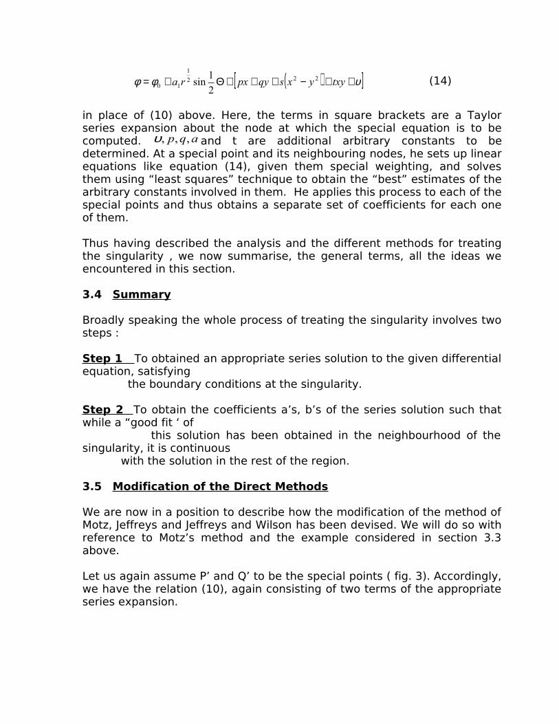
( )[ ]υφφ ++−+++Θ+= txyyxsqypxra 222
1
10 2
1sin (14)
in place of (10) above. Here, the terms in square brackets are a Taylor series expansion about the node at which the special equation is to be computed. aqp ,,,υ and t are additional arbitrary constants to be determined. At a special point and its neighbouring nodes, he sets up linear equations like equation (14), given them special weighting, and solves them using “least squares” technique to obtain the “best” estimates of the arbitrary constants involved in them. He applies this process to each of the special points and thus obtains a separate set of coefficients for each one of them.
Thus having described the analysis and the different methods for treating the singularity , we now summarise, the general terms, all the ideas we encountered in this section.
3.4 Summary
Broadly speaking the whole process of treating the singularity involves two steps :
Step 1 To obtained an appropriate series solution to the given differential equation, satisfying the boundary conditions at the singularity.
Step 2 To obtain the coefficients a’s, b’s of the series solution such that while a “good fit ‘ of this solution has been obtained in the neighbourhood of the singularity, it is continuous with the solution in the rest of the region.
3.5 Modification of the Direct Methods
We are now in a position to describe how the modification of the method of Motz, Jeffreys and Jeffreys and Wilson has been devised. We will do so with reference to Motz’s method and the example considered in section 3.3 above.
Let us again assume P’ and Q’ to be the special points ( fig. 3). Accordingly, we have the relation (10), again consisting of two terms of the appropriate series expansion.

Now let ( )0Pφ and ( )0
Qφ be the trial values of φ at the further away nodes P and Q, then in place of (11) we write
( )PpPPP rara Θ+Θ= sinsin 22
12
1
100 φφ
and (A)
( )QQQQQ rara Θ+Θ= sinsin 22
12
1
100 φφ
again these are linear simultaneous equations, but this time the algebraic quantities involved in them are only 1a and 2a . Hence, on solving them we obtain the first estimates of the coefficients 1a and 2a . Let us call them
( )01a and ( )0
2a respectively. Now, corresponding to them the function values at P’ and Q’ from (10) are
( ) ( ) ( ),,,,' sinsin 1
2212
11
101
PpPPPrara Θ+Θ= φφ
and (B)
( ) ( ) ( ),,,,' sinsin 1
2212
11
101
QQQQQrara Θ+Θ= φφ
Relations (B) are no more algebraic special equation. Their right hand side being completely known they are the numerical estimates of the function values at the special points P’ and Q’. Momentarily we fix these estimates at P’ and Q’, and relax the rest of the region using a standard finite difference formula. This gives us fresh estimates ( )1
Pφ and 1Qφ at P and Q
respectively. We repeat the cycle over and over again till finally the process converges. As the only bit of algebra involved here is the solution of the linear simultaneous equations (A) it is easy to programme the whole iteration procedure for automatic computation.
It is easy to see that there can be no difficulty in likewise modifying the methods of Jeffreys and Jeffreys and Wilson.
We have tested the modified versions of Motz’s and Jeffreys and Jeffreys methods on the examples solved by them in their respective works. The results were satisfactory.
3.5 Back to our problem

As this stage we return to our problem already stated in section 3.2, and propose to treat the re-entrant corner occurring in (2) in exactly the same manner as outlined in steps 1 and 2 mentioned in section 3.4.
Hence, as step 1 we proceed to find out the series solution to (2), satisfying the boundary conditions that V=φ on ( )π=ΘAG and ( )π=ΘGB .We transfer the origin to G by using the transformation:
1−= Ps
We thus obtain from (2)
2
2
2
2
1
1
zss ∂∂+
++
∂∂ φφ
On changing this into plane polar coordinates, we get on using 222 zar += and
s
z=Θtan
the equivalent form
0..cos1
112
2
22
2
=
∂Θ∂
Θ∂∂+
∂∂
∂∂
Θ++
Θ∂∂+
∂∂+
∂∂
ss
r
rrrrr
φφφφφ
or ( ) 0sin
coscos111 1
2
2
22
2
=
Θ∂∂Θ−Θ
∂∂++
Θ∂∂+
∂∂+
∂∂ − φφφφφφ
vvr
vvrr (15)
Let the solution to (15) be
( ) ( ) ( ) ( )[ ].......22
102 +Θ++Θ+Θ+Θ= n
n frfrrffrφ (16)
then ( ) ( ) ( ) .......21 12
110
1 ++++++++=∂∂ −++−
nnQ frnfrfrfr
rαααα αααα
( ) ( ) ( )( ) ( )( ) ....1....1211 221
10
12
+−+++++++++−=∂
∂ −+−−n
n frnnfrfrfrr
αααα ααααααααφ
......11
0 +′′+′+′=Θ∂
∂ ++n
n frfrfr αααφ
.......11
02
2
+′′+′′+′′=Θ∂
∂ ++n
n frfrfr αααφ

On substituting these values in (15) we get
( )( ) ( )...coscoscos11 3322
0
2
0
2 +Θ−Θ+Θ−+′′+−++ ∑∑=
−+
=
−+ rrrfrfrnnn
nn
nn
n αααα
( ) 0sincos0 0
11 =Θ
′−Θ+∑ ∑
= =
−+−+
nn
n
mn
n frfrn ααα
On rearrangement we get
( ) ( )[ ] 1001
21
20
20 sincos1 −− Θ′−Θ+++′′++′′ αα ααα rffffrff
( ) ( )[ ] αααα rffffff ΘΘ′+Θ′−Θ−Θ++++′′ cossinsincoscos12 012
0122
2
( ) ( ) ( )[ ]ΘΘ′−ΘΘ′+Θ′−Θ+Θ+−Θ++++′′ 2012
30
2123
23 cossincossinsincoscos1cos23 ffffffff αααα
0...1 =++αr
Since this power series is identically equal to zero, all its co-efficient must vanish separately. Hence
002
0 =+′′ ff αor Θ+Θ= αα cossin 000 baf
Next , ( ) 0sincos1 0012
1 =Θ′−Θ++∂+′′ ffff α
Which gives ( ) ( ) ( ) ( )[ ]Θ−+Θ−−Θ++Θ+= 1cos1sin4
11cos1sin 00111 αααα babaf
Similarly, ( ) ( ) ( ) ( )( ) Θ
++−+
−Θ++Θ++ αα
αααα sin116
21142cos2sin 01
222
aabaf
( ) ( )( ) ( ) ( )[ ],2cos2sin
32
3cos
116
211400
01 Θ−+Θ−+Θ+
+−+− ααα
ααα
babb
And so on.
In our particular problem, the series solution should be such that it
vanishes on ( )π=ΘAG and ( )π=ΘGB . Hence we have 21=α and all 0' =sa .
We can also assume that as many as only two terms of the series expansion would be sufficient for our purposes.

Hence we neglect terms with coefficients 1, ⟩nbn . In this way we are able to
simplify the expression for 210 ,, fff etc.
2cos00
Θ= bf
Θ−=2
1cos
4
101 bf
Θ−
Θ+Θ=
2
1cos
4
1
2
3cos
32
3
2
1cos
12
1102 bbf
103 2
3cos
10
1
2cos
32
3
2
5cos
128
5
2
3cos
30
1
2cos
16
1bbf
Θ+Θ+
Θ+Θ+Θ−=
etc.
Finally on substituting these and several more expressions like this in (16) and remembering that V=φ on the disc AG, we write
Θ
+−+−+−+Θ
+−+−+−+−+=
2
3cos....53535
3032
3
2cos...
256
5
224
5
3280
3
161241 5432
765432
025
21
rrrrr
rrrrrrrr
rbVφ
2
7cos...
1548192
105
315
2
2048
35
2
5cos...
4096
63
841536
35
70128
5 32432
27 2
9 Θ
+−+−+Θ
+−+−− rrr
rrrrr
r
+Θ−Θ
−+Θ
−+−− ...
2
13cos
1048576
3003
2
11cos
3003
4
65536
231
2
9cos...
8192
99
693
2
8192
63 2
152
213
211 rr
rrr
r
2cos...
512
15
224
9
64
3
40
3
32
3
4
1
2
3cos
168
5
256
7
560
27
128
5101
54322
5654322
3
1
Θ
+−+−+−−Θ
−+−+−++ rrrrr
rrrrrr
rb
2
7cos...
308
5
8192
63
105
2
2
5cos...
4096
63
352048
35
70
3 22
11222
9 Θ
−+−+Θ
+−+−− rr
rrr
r
−Θ+Θ
+−− ...
2
11cos
1001
4
2
9cos...
65536
231
231
2 2
15
2
13 rrr (17)
In view of the slow convergence of the series expansion, we went as far as 7f .
Thus having obtained the series expansion, we have finished with step 1. We now proceed ahead to step 2 . Here, we have to obtain suitable estimates of the coefficients 0b and 1b occurring in the series expansion (17). We have employed the modified versions of the Motz’s and the

Jeffreys and Jeffrey’s methods towards this end . They have already been described in section 3.5. Hence we now proceed to outline the numerical details and the sets of results we have obtained.
3.7. The numerical details
Let the radius AM of the cylinder be 35 units and its semi length 5=AQ
units (fig. 1). Further, let us cover the region AGMPQ by a square net of
mesh length = 61 . Now , if the potential on the disc be 1000, then we set
1000=V in (17).
In figure 4 we have drawn a small portion of the region near the singularity.
N7N6
Q SRN2
N5 NBN4
G P N1
N3
A
B
Figure 4.With reference to this figure we would point out the special points and the further away nodes considered for the different results . In all , nine sets of results, have been worked out – eight by the modified Jeffreys and Jeffreys method (briefly called m-j.j) and only one by the modified Motz’s method (called m-M). The details are as shown on the next page.
Table 1
No. Method
Special Points
Further away nodes
Coefficientb0
Coefficientb1
Number of
iterations
1 m-J.J. P, Q, R, S N1 N4 N6 N8 -1415042
- 8
2 m-J.J. P, Q, R, S N1 N4 N6 N8 -1465.42 42.60 103 m-J.J. P, Q, R, S N1 N2 N3 N5 N6
N7-1421.27 - 10
4 m-J.J. P, Q, R, S N1 N2 N3 N5 N6 -1400.85 58.04 10

N75 m-J.J. P, Q, R, S N1 TO N8 -1418.74 - 96 m-J.J. P, Q, R, S N1 TO N8 -1432.60 32.93 107 m-J.J. P, Q, R, S N1 TO N9 1431.74 - 98 m-J.J. P, Q, R, S N1 TO N9 1440.16 36.99 99 m-M P, R N1, N6 1433.66 117.55 11
Symmetries about the axis of the cylinder and the disc were taken into account in all the versions of the method of Jeffreys and Jeffreys. The equation at N1 was weighted twice while at rest of the nodes they were weighted four times.
The actual results, from all the nine cases above, have been recorded in appendix A(3)I to A(3)IX. For ready convenience, however , we have in fig. 5, a magnified picture of the region near the singularity . At each node are the function values as obtained in the different cases. These cases have already been serially ordered in table I, and the function values from them have been arranged in the same order for example , the function values at the top correspond to the case marked I in table I.
Table I clearly indicates the special points considered in each version of the methods listed there. They are called special points because special equations are used at them. In contrast , at rest of the nodes, ordinary finite difference equations are used. The five-point finite difference representation to (2) which we have used here is
=−+
−++
+ 04
21
21 043
021
0
φφφφφp
h
p
h(18)
where the subscripts have their usual meaning.

307302307307307305306304295
265261265266265264263255
216211215216215214214213208
161157160161161160160159155
392387392392392390391389376
340334340341340338339337327
276270275277276274274273266
204199204205204202203202198
504497503504504501502500480
439431438439439436437435421
656648655655655652654651614
808802808807808805807804787
572562572572572568570567548
755742754751754748752747728
355347354356354352352350342
259251258261258256256255251
460449459461459456457454446
608592607610608602604600597
325314324329324321321319317
399379396407397393392390391
307302307307307305306304295
444427441453442439437436444
105102105105105104104104101
132128132133132131131130128
165160164166164163163162160
201194200204200199198197196
235225234239234232231230231
252241250254251248248247249
Figure 5.

-.00019 B 0 +.00075B 1-.00422B 0 +.00018B 1 -.00019B 0 -.00038B 1
.00271B 0 +.00047B 1.01224B 0 +.00216B 1 -.04626B 0 +.00045B 1 .01193B 0 -00143B 1
.00219B 0 -.00009B 1
-.02900B 0 +.00280B 1-.00245B0+.00049B1
Figure 6.
0.280.320.280.320.280.310.290.300.40
5.96.26.05.95.95.96.06.06.06.0
0.280.280.260.280.270.260.270.280.24
-3.8-3.8-3.8-3.7-3.8-3.8-3.8-3.8-3.8
-3.1-3.2-3.1-3.1-3.1-3.2-3.1-3.2-3.2
3.43.53.43.43.43.43.43.53.742.0
-17.066.017.0
Figure 7.
The truncation error, involved in (18), is given by
...5123 5
0
05
0
5
40
04
40
044
30
03
0
4
+∂∂
∠+
∂∂
+∂∂
+∂∂
∠ PP
h
Zp
h
PP
h φφφφ(19)

Using ф as given by the series solution (17), we can obtain an estimate of this error at different nodes in each version of the above methods. The first three terms of (19), viz. those, which are in square brackets, are the principal contributors to this error.Fig. 6 shows its magnitude, in terms of the coefficients 0b and 1b . at some of the nodes in the vicinity of the singularity. On substituting the values of
1b and 1b from table I, we obtain the numerical estimate of this error at each node. It is shown in fig. 7. The error, corresponding to each method, has been arranged at a node in the same serial order as the method itself in table I.
It is interesting to find from fig.7 that in all the nine cases , the value of this error at each node is almost the same. It may indicate that in order to take account of the singularity it does not really matter whether we consider the series solution (17) as far as term in 1b or just in 0b .
The four nodes P, Q, R and S are obviously, the dangerous ones .As was expected, the errors are large at them all.
In Motz’s method (case 9, table I), only two of these four nodes have been dealt with rather squarely. They are P and R (fig. 7), where special equations have been used. However, at Q and S, where the finite difference equations have been used, the solution is bound to be more inaccurate, and the local neighbourhood will also be affected , appropriately.
In all the versions of the method of Jeffreys and Jeffreys (cases 1 to 8, table I), special equations have been used at all the four nodes P,Q,R and S . In this sense, this method can be regarded to promise better results than Motz’s method. In theorem I, section 90, Milne (1957) has given an expression for estimating the upper bound of the error in the finite difference solution of the Laplace’s equation. If we choose to use the same expression here as well, then it appears that the solutions obtained from the method of Jeffreys and Jeffreys have a maximum error of about 13 units.
In appendix A(3) X is the solution obtained by ignoring the presence of singularity. It is included here for purposes of comparison.
Concluding Remarks

We could not try Wilson’s method here. In addition to the series expansion about the corner, it also required a Taylor series about the node. It is a limitation with this method.
So far we did not make any mention of Wood’s method. However, we did try his method over our problem, but found that it did not converge. With Laplacian operator it converges, even under such situations as we had here. This behavior of the method needs investigation. We have not attempted to explore it.
CHAPTER IV
EXTENTION OF MILNE’S METHOD TO BIHARMONIC EQUATION
4.1. Introduction
Eigenvalue problems arise in a variety of ways in Mathematical Physics, and whether they appear associated with the ordinary or the partial differential equations, the finite difference procedure of their solution is to reduce them to a matrix of the form
( ) 0=− ii xIA λ (1)
and then calculate the latent roots iλ and vectors ix of the matrix A.
This sort of reduction of a continuous problem to one of discrete nature is the basis of the finite difference theory. The finite difference approximation need be reasonably accurate therefore, otherwise, the ill effects of discretisation are sometimes evident even in the least latent roots.
Milne (1957) has proposed a method whereby, using not too refined relaxation patterns for the different differential operators, it is possible to obtain results which would be better than those which one would ordinarily obtain from (1). He has applied it to the eigenvalue problems in the

ordinary differential equations and the partial differential equations with the two dimensional Laplacian operator. In this chapter the same technique has been extended to the partial differential equations associated with the bi-harmonic operator
4
4
22
4
4
44 2
yyxx ∂∂+
∂∂∂+
∂∂≡∇
in two dimensions.
4.2. The Analysis
Associated with appropriate boundary conditions , the general equation governing the free vibrations in a plate is
uPu i44 =∇ (2)
where ( )yxuu ,= is the transverse displacement of the plate, held in the x-y plane; and pi, called the eigenvalues, are purely numerical quantities such that a non-trivial solution of (2) is valid. The problem is to determine the eigenvalue iP .
Let us consider an arbitrary function ( )tyxww ,,= satisfying the parabolic equation
wct
w 22∇=∂∂
(3)
Differentiating (3) we get the sequence
wct
w 442
2
∇=∂∂
(4)
wct
w 663
3
∇=∂∂
(5)
Let us cover the plate with a square mesh of width h and let k be the direction of t. Then by Taylor’s Theorem, we have

( ) ( ) ( ) ...12
722
4
44
3
33
2
22 +
∂∂+
∂∂+
∂∂=++−+
t
wk
t
wk
t
wktwktwktw
...12
7 884663442 +∇+∇+∇= wckwckwck
...15552
7
216
1
36
1 886644 +∇+∇+∇= whwhwh
(6) where
226 hkc = (7)
Substituting it in (6) and neglecting higher order terms in h we get
( ) uhukPckPc 442
36
112
2222
∇=+− −−
or uuhPh
2
644
22
136
−=∇
−
Employing a suitable relaxation pattern for 44∇h we obtain a matrix for the region of the plate. Let iλ be the latent roots of this matrix,then
2
6
22
136
−=
− iPh
i λ
or
−−=
61622 i
i mPhλ
(8)
which gives the required eigenvalues ip
4.3Applications of the formula to rectangular plates
A coarse relaxation pattern for 44∇h as
12 -8 2
1 -8 +20 -8 12 -8 2
1

and for a rectangular plate, supported at its four edges, λ is given by
−−
βπ
απ hnhm
coscos24 (9)
Where α and β the length and breadth of the plate and m, n are integers. Substituting it in (8) we get
+−=
βπ
απ
2sin
2sin
3
216 2222 hnhm
mPh (10)
or ...22
1086 6
6
42
42
24
24
6
646
22
2224
2
2
2
222 +
+++++
+=
ββαβααα
βαπ
βαπ nnmnmmhhnmnm
P (11)
The similar expression as would be obtained direct from (9) is
...3612 6
6
6
646
4
4
4
424
2
2
2
22 +
++
+−
+
∂ βαπ
βαπ
βπ nmhnmhnm
(12)
The first term in the series (11) and (12) are the true values of 2P , the remaining terms being the error terms in both the series.
The remaining terms being the error terms in both the series are, obviously, the dominant ones, and it is easy to see that the first error terms in (11) are smaller than their counterparts in (12) expect when m = n in a square plate. Hence it is clear that (11) will give a better estimate of 2P as obtained from (11) and (12) for a 2 x 3 rectangular plate :
No True value of P 2
H = 1/4 H = 1/8 H=1/12
From (11)
From(12) From(11)
From (12)
From (11)
From (12)
12345
3.564 6.85410.96612.33714.256
3.593 6.97011.07812.60014.725
3.526 6.72310.99412.40114.370
3.5716.88210.99412.40114.370
3.554 6.82110.83812.20314.105
3.5656.85710.96912.34414.269
3.5636.85010.95112.32214.239

While the true value were computed by ( )222
2 9436
nmP += π
The approximate values were calculated from (9) and (10) not from the series (11) and (12). It is easy to see that first- column-approximate- values for each h are closer to the true values than the second-column-approximate values.
So far we employed a poor relaxation pattern for 44∇h . However, using a better relaxation pattern we can expect highly improved results. One such relaxation pattern is
1 1 1 1 -2 -10 -2 1 443 ∇h = 1 -10 36 -10 1 ( )60 h
1 -2 -10 -2 1 1 1 1
we have taken it from Collatx (1959) with this relaxation pattern for 44∇h and time interval defined by (7) we can approximate (4) to a high order of accuracy – the error involved is ( )80 h .* Using this relaxation pattern and taking h = ¼ we again solve the above problem. The least latent root of the resulting matrix is found to be 0.0478093 by Lanozos’s method. We substitute this value in formula (8).
−−=
6
0478093.16122 nPh
)(.9635577861n - = 8)6x(.037122 +=
.2227368 = 3.56379 P 2 =
This is an agreeable estimate.
If we choose not to use formula (8) , then a value of the same order Of
accuracy and with 4
1=h could be found out by Lanozos’s iterative
* Let us denote the operator 1 1 1 1 -2 -10 -2 1 1 -10 36 -10 1 1 -2 -10 -2 1 1 1 1
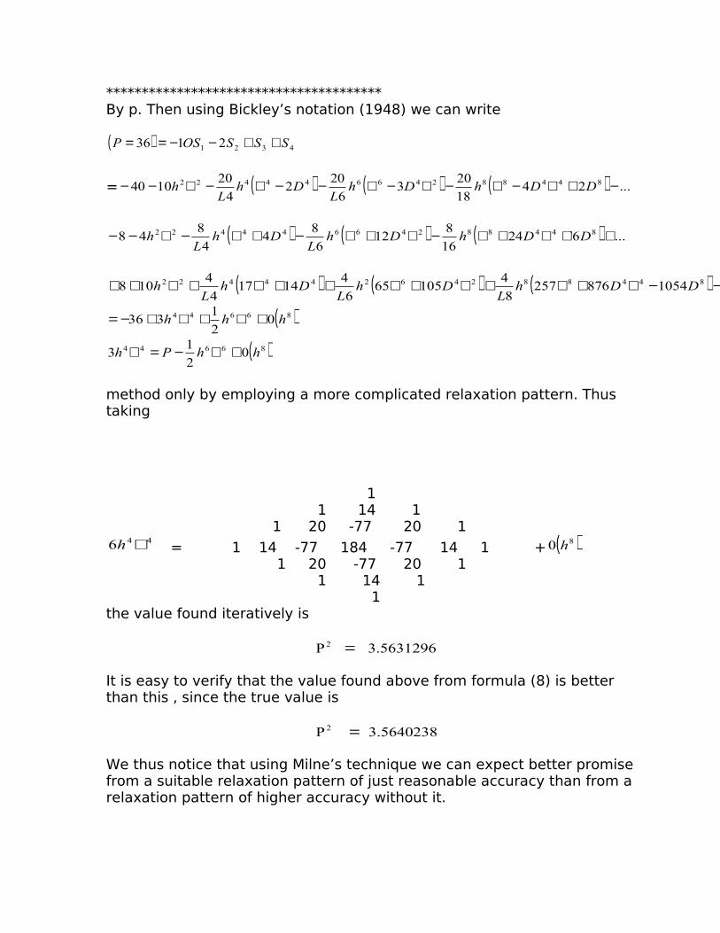
***************************************By p. Then using Bickley’s notation (1948) we can write
( ) 4321 2136 SSSOSP ++−−==
= ( ) ( ) ( ) ...2418
203
6
202
4
201040 84488246644422 −+∇−∇−∇−∇−−∇−∇−− DDhDh
LDh
Lh
( ) ( ) ( ) ...6̀2416
812
6
84
4
848 84488246644422 ++∇+∇−∇+∇−+∇−∇−− DDhDh
LDh
Lh
( ) ( ) ( ) ...10548762578
410565
6
41417
4
4108 84488246244422 −−∇+∇+∇+∇++∇+∇++ DDh
LDh
LDh
Lh
( )86644 02
1336 hhh +∇+∇+−=
( )86644 02
13 hhPh +∇−=∇
method only by employing a more complicated relaxation pattern. Thus taking
1 1 14 1 1 20 -77 20 1
446 ∇h = 1 14 -77 184 -77 14 1 + ( )80 h 1 20 -77 20 1 1 14 1 1the value found iteratively is
3.5631296 P2 =
It is easy to verify that the value found above from formula (8) is better than this , since the true value is
3.5640238 P 2 =
We thus notice that using Milne’s technique we can expect better promise from a suitable relaxation pattern of just reasonable accuracy than from a relaxation pattern of higher accuracy without it.

************************************Substituting it in (4) we have
( ) ( ) ( ) ( ) wckwckwhhPh
cktwktwtkw 884663864
4
42
12
70
2
1
322 ∇+∇+
+∇−=++−+=
( ) ( )862242
4
42
0663
hwkchck
Pwh
ck +∇−−=
= ( )84
42
03
hPwh
ck +
on using (7).
CHAPTER V
NUMERICAL SOLUTION OF TWO FREDHOLM TYPEINTEGRAL EQUATIONS OF SECOND KIND
5.1. Introduction
Most problem in Mathematical physics are stated in the form of differential equations and the standard methods of their solution present an interesting field of study. While the method of solving the given differential equation directly , by analytical or numerical methods, still continues to hold its well-established place, another method has been developed during the recent decades. It calls for transforming the given differential equation into a suitable integral equation whose solution is then obtained by affecting the integration involved in it. The boundary conditions are implicitly inherent in the integral equation and are not expressed separately as in a differential equation. Many boundary-value problems in Mathematical-physics are therefore, actually solved through integral equations, and in particular , the elliptic equations are often analysed through non-homogeneous Fredholm type integral equations of the second kind.
In general , the solution of an integral equation by purely analytical methods is not always possible, recourse, therefore, is taken to numerical methods.
In this chapter we have presented the numerical solution of two such integral equations. They are both Fredholm type non-homogeneous integral equations of the second kind, and we have taken them from the analytical works of Sneddon (1962 a) and Srivastav (1963). Their kernels are interesting and they have been briefly explained in the next section. Their numerical evaluation is, in fact , the special feature of this chapter. In solving the integral equation itself, we have employed the direct method which according to Scarborough (1958) was suggested by Goursat and later developed by Nystrom. It replaces the given integral equation by a finite set of simultaneous equations in the unknown function at discrete points.
5.2. A brief description of the Integral equations
As already pointed out, two integral equations have been considered in this chapter. The importance of the integral equation I lies in the fact that the integrand of its kernel has a pole at its lower limit of integration, and the

singularity arising from it requires suitable analytic treatment. It has been done in two ways and their numerical results compare very well.
The kernel of integral equation II has the same form of singularity as that of integral equation I, but in addition it is of special computational interest as well. The integrand of its kernel involves subtracting two functions which are close to each other in magnitude.
The loss of significant figures in this way is one of the serious sources of error in numerical work. The technique adopted here to treat such awkward situation is of general applicability and when a digital computer is available, it is convenient as well. It is interesting to see that in this way, accurate results have actually been obtained.
Both the integral equations are typical examples of their respective types. The integrations involved in the kernels have been evaluated using the standard Gauss-type quadrature formulae, while the integrations in the actual integral equation have performed by suitable Newton-Cotes-type formulae. The choice of these quadrature formulae has the basis that while Gauss-type formulae are well known for their high order accuracy, the Newton-Cotes type formulae are best suited when values of the wanted function are required at equal intervals of the variable.
5.3. Integral Equation I
Sneddon (1962 a) applies the dual series relations technique to the determination of the electrostatics field inside an infinite hollow- earthed cylinder of radius a containing an electrified circular disc of unit radius situated with its centre on the axis of the cylinder and its plane perpendicular to that axis. The problem is eventually reduced to that of solving a Fredhdm integral equation of the second kind for the auxiliary function g(t). It is
( ) ( ) ( )∫ ≤≤+=1
010,,1 tdnutKkngtg (5.3.1)
where the kernel is
( ) ( )( )∫
∞
=
0 0
02
coshcosh4
, dwa
uw
a
tw
wI
wK
autK
π (5.3.2)
where ( )wK0 and ( )wI 0 are modified Bessel functions.

It is easy to see that the integrand in the kernel has a pole at the lower limit, because
( )( ) 0,
0
0 =∞→ atxxI
xK
But we can subtract out the singularity using the fact
( ) ( ) ( ) ( )∑∞
=
+++++Ι+−−=Κ
1
2
00
1...
3
1
2
11
2/2lnln
r
r
rLrLr
xxrxx (5.3.3)
where γ is the Euler’s constant (=0.5772156649……)
we can write (5.3.3) as
( )( ) ( )
( )∑∞
=
++++
Ι++=+
ΙΚ
1
2
00
0 1...
3
1
2
11
2/12lnln
r
r
rLrLr
x
xrx
x
x (5.3.4.)
Remembering that ( ) ( )∑∞
= +=Ι
0
2
0 1
2/
r
r
LrLr
xx (5.3.5)
We can see that the right hand side of (5.3.4) is now well behaved at x = 0. On this basis we can write the kernel
( ) ( )( ) dw
a
uw
a
tw
w
w
ant ∫
∞
ΙΚ
=Κ0 0
02
coshcosh4
,π (5.3.6)
( )SRQPa
++−=2
4
π
Where
( ) ( ) ( )
( ) dwa
uw
a
tw
w
wwwP coshcosh
ln1
00
00∫ ΙΙ+Κ
= (5.3.7)
( ) dwa
uw
a
twwQ coshcoshln
1
0∫= (5.3.8)
( )
( )∫ ΙΚ
=q
dwa
uw
a
tw
w
wR
00
0 coscosh (5.3.9)

and ( )
( ) dwa
uw
a
tw
w
wS
q∫∞
ΙΚ
= coshcosh0
0 (5.3.10)
We first attend to the integral Q. We can evaluate it by term-by-term integration of the power series expansion of the integrand, thus
∫ ∑ ∑− =
+
=
1
00 0
2
222
2
2
ln22m n
n
nnm
m
m
wdwnLa
uw
mLa
tQ
( )∑ ∑= − ++
−=0 0
22
2
2
2
21222m nn
n
m
m
nLanm
u
mLa
t (5.3.11)
Next, the integrations in P, R and S can be obtained by the Gauss-type quadrature formulae, using the zeros and weight given in AMS37 (1954). To suit limits of integration appropriate to these zeros and weights we make a change in the independent variable. Accordingly, we obtain
( ) ( )dz
a
uz
a
tzz
zzz
P ∫+
−
++
+Ι
+Ι
++
+Κ
=1
1
0
00
2
1cosh
2
1cosh
2
12
1
2
1ln
2
1
2
1 (5.3.12)
∫+
−
++−
++−
++−Ι
++−Κ
−=1
1
0
0
2
1
2
1cosh
2
1
2
1cosh
2
1
2
12
1
2
1
2
1dz
az
a
a
uaz
a
a
ta
za
az
a
qR
(5.3.13)
dzquta
az
a
uq
uta
az
a
t
quta
az
quta
az
eeuta
aS zz
+
−−
+
−−
+
−−Ι
+
−−Κ
−−= ∫
∞−
2cos
2cos
2
22 0
0
0
(5.3.14)
In the determination q the method of trial and error is best suited. It was found that q = 8 is a right value ; and it has been used in evaluating R and S above.

5.31. The Numerical Procedure
In order to determine g(t) in (5.3.1) at equidistant values of t , we cannot use the Gauss-Legendre quadrature formula to evaluate the integration involved . Instead we use a Newton-Cotes formula as pointed out earlier. We divide the range of integration , i.e. 0 to 1, into eight equal intervals so that we could use the formula
[ ]∫ ++++++++=1
0 876543210 732123214321232745
2ppppppppp
hpdx (5.3.15)
where rP are the ordinates and h = 1/8 in this case.
This division of the range of integration leads us to the finding out of the Kernel ( )utK , at points which are clearly the different combinations of the
values of t and u as picked up from 8
,r
ut = t, u, where r = 0, 1, 2, ….8.
The rest of the procedure is straight forward and the values of the integrals P,Q,R and S for a = 1.2, 1.3, 1.4 have been tabulated in appendices A(5)I, A(5)II, A(5)III, A(5)IV; the values of the kernel K(t, u) have been tabulated in appendix A(5)V and finally the wanted function g(t) has been tabulated in appendix A(5)VI.
5.32. The Alternate Approach
The kernel as presented in equation (5.3.2) has a comparatively simple form for straight forward evaluation as shown above . However, on applying a short analysis we can write the kernel in another form, viz.
( )
−++
−−+
++=Κ
a
ulltk
a
ulltk
a
utk
aut 222
1,
2π(5.3.16)
where ( ) ( ) ( ) ( )a
a
a
adz
z
zek
zz 1212
,0
02
0
+<<−ΙΚ
= ∫∞ − ζζ ζ (5.3.17)
To evaluate ( )ζk we write
( ) ( )( ) dzz
zeek
zz
0
02
0 ΙΚ
= ∫∞ −ζζ
= CBA −+ (5.3.18)

where ( ) ( )( )
( ) dzz
zzeA z
0
01
0
2 ln
ΙΚ
= ∫ −ζ (5.3.19)
( ) zdzeB z ln1
0
2∫ −= ζ (5.3.20)
and ( )
( ) dzz
zeeC
zz
0
02
1 ΙΚ
= ∫∞ −ζ (5.3.21)
The evaluation of the integrals A and C presents no difficulty. After a change of the independent variable they could be written as
dtt
ttt
eeAt
+Ι
+
+Ι+
+Κ
= ∫+
−
−−
2
12
1ln
2
1
2
1
2
1
0
001
1
2
51
21
ζ
(5.3.22)
dtt
te
ee
C
t
t
+Ι
+Κ
= ∫∞ −
−
1
1
0
0/2
0
2
ζ
ζζ
ζζ
(5.3.23)
which can now be evaluated using the Gauss-Legendre and Gauss-Laguerre formulae of quadrature. It is in fact the evaluation of B, which presents some difficulty, for ordinarily, in diverges for 2≠ζ . But on using the formula in 324S , case 81a, page 81, Integraltafel Springer Verlag, 1958, we can write
( )( )
( )∫∫ ≠+−−−==
−− 1
0
21
0
2 2,1
2
1ln ζ
ζ
ζζ dz
z
ezdzeB
zz
On changing the independent variable we can write
( )( )( )∫
+
−
+−
≠+
+−−−=
1
1
12/1
2,1
1
2
1 ζζ
ζ
dtt
eB
t
We can now evaluate it for all 2≠ζ using the Gaussian formula of quadrature.
However, for the particular case when 2=ζ , we have from (5.3.20) direct
1ln1
0−==∫ dzzB
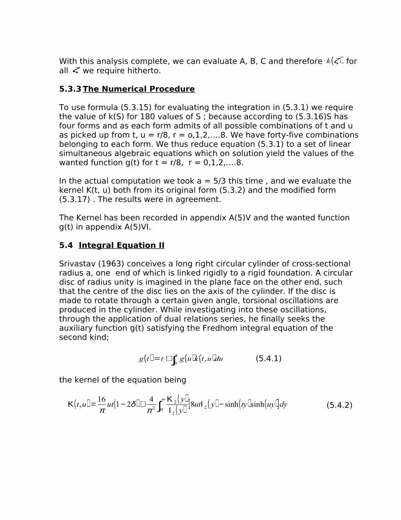
With this analysis complete, we can evaluate A, B, C and therefore ( )ζk for all ζ we require hitherto.
5.3.3The Numerical Procedure
To use formula (5.3.15) for evaluating the integration in (5.3.1) we require the value of k(S) for 180 values of S ; because according to (5.3.16)S has four forms and as each form admits of all possible combinations of t and u as picked up from t, u = r/8, r = o,1,2,….8. We have forty-five combinations belonging to each form. We thus reduce equation (5.3.1) to a set of linear simultaneous algebraic equations which on solution yield the values of the wanted function g(t) for t = r/8, r = 0,1,2,….8.
In the actual computation we took a = 5/3 this time , and we evaluate the kernel K(t, u) both from its original form (5.3.2) and the modified form (5.3.17) . The results were in agreement.
The Kernel has been recorded in appendix A(5)V and the wanted function g(t) in appendix A(5)VI.
5.4 Integral Equation II
Srivastav (1963) conceives a long right circular cylinder of cross-sectional radius a, one end of which is linked rigidly to a rigid foundation. A circular disc of radius unity is imagined in the plane face on the other end, such that the centre of the disc lies on the axis of the cylinder. If the disc is made to rotate through a certain given angle, torsional oscillations are produced in the cylinder. While investigating into these oscillations, through the application of dual relations series, he finally seeks the auxiliary function g(t) satisfying the Fredhom integral equation of the second kind;
( ) ( ) ( )∫+=c
duutkugttg0
, (5.4.1)
the kernel of the equation being
( ) ( ) ( )( ) ( ) ( ) ( )[ ]∫
∞−Ι
ΙΚ+−=Κ
0 22
22
sinhsinh84
2116
, dyuytyyuty
yutut
πδ
π (5.4.2)

where c = 1/a, 8 = length of cylinder and y2Κ and y2Ι are modified Bessel functions.
It is easy to see that the integrand in the kernel (5.4.2) has the same form of singularity as was encountered in integral equation I above. Hence, we can treat it in exactly the same way, and there is nothing exciting about it so far. But, as pointed out earlier , the kernel is really interesting from a computational point of view. To appreciate it, Let us have a look at the function within square brackets in the integrand in (5.4.2). Using Taylor expansions and setting
utP +=
utQ −=
( ) ( ) ( )yqpyut 222
2 28 Ι−=Ι
( ) ( )∑∞
=
+
+∠∠−=
0
2222
2
2/2
s
s
ss
yqp
( ) ( ) ( ) ....1536
1
48
1
4
1 622422222 +−+−+−= yqpyqpyqp
and
( ) ( ) ( )qypyuyty coshcosh2
1sinhsinh −=
( ) ( )
+−+−+−= ...
1440
1
48
1
4
1 666444222 yqpyqpyqp
Now, it is obvious that the principal terms in the two expansions are the same, consequently, when one is subtracted from the other, a wholesale loss of significant figures is bound to happen. Unless it is checked, the results would be terribly inaccurate. The best way to deal with this sort of situation is to cancel these terms analytically, and to use the rest of the power series in place of the function in question. Thus we replace the function

( ) ( ) ( )uztyyut sinhsinh8 2 −Ι
By its power series equivalent
∑ ∑ ∑ ∑∞
=
∞
=
∞
=
∞
=
+++++++−
−+∠∠
−+∠∠
−+∠
−+∠+∠0 0 0 0
62125421234232422
......12
.
512
.
332
.
31
.2
2 s s s s
ssssssss
s
ytu
s
ytu
s
ytu
ss
yut
(5.4.3)
The technique works efficiently with digital computers.
Thus having defined the basis of our approach to carry out the integration involved in the kernel (5.4.2) in the following manner,
( ) ( ) [ ]EDCBAutut −−+−+−=Κ2
421
16,
πδ
π (5.4.4)
where
( ) ( ) ( )( ) ( ) ( ) ( )[ ]∫ −Ι
ΙΙ+Κ=
1
0 22
22 sinsinh8ln
dyuytyyuty
yyyA
( ) ( )
∫+
−
++−
+Ι
+Ι
++
+Κ
=1
1
2
2
2
2
1sinh
2
1sinh
2
18
2
12
1ln
2
1
2
1dp
puptput
p
pp
(5.4.5)
( ) ( ) ( )[ ]∫ −Ι=1
0 2 lnsinhsinh8 ydyuytyyutB
∫ ∑ ∑ ∑
−
+∠∠−
+∠−
+∠+∠=
=
∞
=
∞
=
+++++−1
00 0 0
421234232422
ln....12
.
332
.
31
.2
2ydy
s
ytu
s
ytu
ss
yut
s s s
ssssss
( ) ( ) ( )
+
+∠+∠+
+∠++
+∠+∠+−= ∑ ∑ ∑
=
∞
=
∞
=
+
0 0 02
22
2
22
22...
125233252312.52
1
2
1
s s s
ss
s ss
tu
ss
t
sssut
(5.4.6)
by term by term integration.

( )∫∞Κ=
1 28 dyyutC
( )
( ) ( ) ( )dyuytyy
yD
r
∫ ΙΚ
=1
2
2 sinhsinh
and
( )( ) ( ) ( )dyuytyy
yE
r∫∞
ΙΚ
= sinhsinh2
2
To evaluate C, we use the fact
( ) ( ) ( ).2 120 yyy ′Κ−=Κ+Κ
integrating it , we obtain
( ) ( ) ( )∫ ∫∞
∞Κ=Κ+Κ
11 120 12dyydyy
or ( ) ( ) ( )∫∫∞∞Κ−Κ=Κ
1 01 12 12 dyydyy
=2(0.6019072302)-(0.328286478)1*
=0.8875527982
ThusC=8ut (0.875527982 ) (5.4.7)
Again, by the method of trial and error it was found that r=4 is a suitable value. Hence we write
( )( ) ( ) ( )∫ Ι
Κ=4
12
2 sinhsinh dyuytyy
yD
( ) ( )
dxxuxt
x
x
2
53sinh
2
53sinh
2
532
53
2
3 1
1
2
2 ++
+Ι
+Κ
= ∫+
−
(5.4.8)
and lastly
1 ( )∫∞
=1 0 ;328286478.0dyyK (Phil. Mag. Vol 20, 1935(7) Bickley and Nayler, pp. 343-347
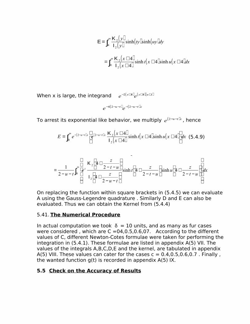
( )( ) ( ) ( )∫
∞
ΙΚ
=Ε4
2
2 sinhsinh dyuytyy
y
( )
( ) ( ) ( )∫∞
+++Ι+Κ=
02
2 4sinh4sinh4
4dxxuxt
x
x
When x is large, the integrand ( ) ( )( )tuxx ee +++− 442
( ) ( )xtutu ee −−−−−− 224
To arrest its exponential like behavior, we multiply ( )xtue −−2 , hence
( ) ( ) ( )( ) ( ) ( ) dxxuxtx
xeeE xtuxtu
++
+Ι+Κ
= −−∞ −−−∫ 4sinh4sinh4
4
2
22
0
2 (5.4.9)
∫∞
−−+
−−+
−−+Ι
−−+Κ
−−=
0
2
2
24sinh
24sinh
24
24
2
1dx
ut
zu
ut
zt
tu
zut
z
etu
z
On replacing the function within square brackets in (5.4.5) we can evaluate A using the Gauss-Legendre quadrature . Similarly D and E can also be evaluated. Thus we can obtain the Kernel from (5.4.4)
5.41. The Numerical Procedure
In actual computation we took δ = 10 units, and as many as fur cases were considered , which are C =04,0.5,0.6,07. According to the different values of C, different Newton-Cotes formulae were taken for performing the integration in (5.4.1). These formulae are listed in appendix A(5) VII. The values of the integrals A,B,C,D,E and the kernel, are tabulated in appendix A(5) VIII. These values can cater for the cases c = 0.4,0.5,0.6,0.7 . Finally , the wanted function g(t) is recorded in appendix A(5) IX.
5.5 Check on the Accuracy of Results

It is important that numerical results should be checked by a suitable method . Accordingly, all the results obtained above, in both the integral equations, have been checked and found to be reliable.
In both the integral equations it is the evaluation of the kernels which is pretty involved . Hence we need be sure about their accurate evaluation. We have already pointed out that Gaussian quadrature has been used in determining the kernels. This sort of quadrature is highly accurate and the best way to check its results is to re-evaluate the integral using a different number of ordinates this time. If the two results agree then only they are reliable This well-known method was employed in both the integral equations and checks were made for certain values of t and u, and the trial and error method referred to above for the determination of the limits q and r is infact this basis.
In addition to this , the kernel in integral equation I has been evaluated in an alternate way as well; and the agreement in the two results indicates their reliability.
On differencing the wanted function g(t) of integral equation I, we find it to be well-behaved, which is in accordance with the estimates of Sneddon.
To check the wanted function g(t) of integral equation II, we find that Srivastav points out that it is possible to approximate the function g(t) by a polynomial in odd powers of t. Hence we write
( )5
3
3
21
+
+
=
c
t
c
t
c
ttg γγγ (5..5.1)
and
( )
Γ=c
ttg 1 (5.5.2)
as well, as good fits. If a least square fitting be done, we find that the coefficients 32,1 ,γγγ and 1Γ are as follows
No. Coeffs c = 0.4 c = 0.5 c = 0.6
1 Γ1 +0.13103 +0.09939 +0.07497
2 γ1 +0.13171 +0.08929 +0.07806
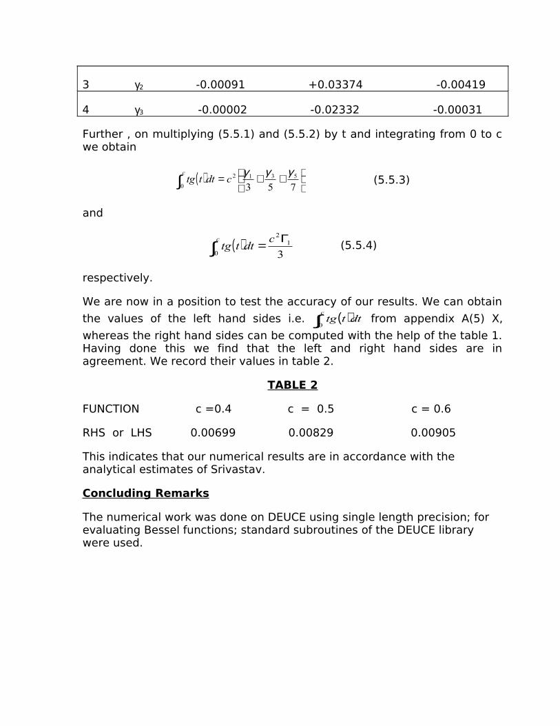
3 γ2 -0.00091 +0.03374 -0.00419
4 γ3 -0.00002 -0.02332 -0.00031
Further , on multiplying (5.5.1) and (5.5.2) by t and integrating from 0 to c we obtain
( )∫
++=
ccdtttg
0
5312
753
γγγ (5.5.3)
and
( )∫Γ
=c c
dtttg0
12
3 (5.5.4)
respectively.
We are now in a position to test the accuracy of our results. We can obtain
the values of the left hand sides i.e. ( )∫c
dtttg0
from appendix A(5) X,
whereas the right hand sides can be computed with the help of the table 1. Having done this we find that the left and right hand sides are in agreement. We record their values in table 2.
TABLE 2
FUNCTION c =0.4 c = 0.5 c = 0.6
RHS or LHS 0.00699 0.00829 0.00905
This indicates that our numerical results are in accordance with the analytical estimates of Srivastav.
Concluding Remarks
The numerical work was done on DEUCE using single length precision; for evaluating Bessel functions; standard subroutines of the DEUCE library were used.

APPENDIX A(2) I
Of the four parts into which the programme is divided, part I is the most important. Hence a flow chart of only this part is given on the following page. In accordance with the relaxation patterns developed in chapter I, a typical node has 12 points associated with it . In the flow chart they have been referred to as the 12 associates of the node. In addition the mag. TypesDGO10002 and DGO10003 have been referred to as Mag. Tapes I and II respectively. The chart indicates the major step of the programme.

Read the 12 parameters
Read description of 1 row (column)
Is a description of 5 consecutive rows (cols.)ready in store for processing
Start processing nodes of the middle row (cols.)
Write on Mag. tape II(i) number of nodes in this row (column),
(ii) abscissa (ordinate) of each node,(iii) its type.
Find the number of non-O-type nodes in row (col)
Find position of each node and its 12 associates from y-axis (x-axis)
Find position of each non-O type node and its 12 associates from y-axis (x ax is)
Find the boundaries in case any of 12 associates of a node is intercepted
Find coeffic ients of difference equation
Form the difference equation
Write them on Mag. tape I
Upgrade the data(a description of only 4 consecutive rows (cols .) is held in the machine at this moment)
Have all rows (columns) been exhausted
Write the no. of diff. equations formed and bandwidth on Mag. tape I
Write parameters required in subsequent parts on Mag tape II
No
No
Yes
Yes
End

APPENDIX A(2) II
A failure could happen either through a fault in the procedures or in the data. Whenever it happens, message is sent out by the monitor typewriter. It gives the node, the row (column) to which it belongs, as also the failure number. Description of the failures is ;
Failures 1-4 refer to a node whose one arm is interrupted by a Neumann boundary;
1. Users procedure DERV is incorrectly evaluating the angle which the normal gradient makes with the x-axis.
2. Incorrect description of the mesh around this node
3. m<0, the extra node is not available in the region
4. m>0, the extra node is not available in the region.
Failures 5-9 refer to a node whose two arms are intercepted by the Neumann boundary;
5. None of the two extra nodes is available in the region.
6. Users procedure DERV is incorrectly calculating the angle.
7,8,9. Incorrect description of mesh around this node.
Failure 10 . Incorrect description of mesh around a node whose arm(s) is (are) interrupted by Dirichlet boundary.

APPENDIX A(3) I
m-JJCase 1.B0 = -1415.42
0 0 0 0 0 0 0 0 0 0 0
0 0 0 0 0 0 0 0 0 0 1 1 1 1 0 0 0 0 0 0 1 1 1 1 1 1 0 0 0 0 2 2 2 1 1 1 1 0 0 0 2 2 2 2 2 1 1 1 0 0 3 3 3 2 2 2 1 1 0 0 4 4 4 3 3 2 2 1 0 0 5 5 4 4 3 3 2 1 1 0 6 6 6 5 4 4 3 2 1 0 8 8 7 6 6 4 3 2 1 0 10 10 9 8 7 6 4 3 1 0 13 13 12 11 9 7 6 4 2 0 17 16 15 14 12 9 7 5 2 0 22 21 19 17 15 12 9 6 3 0 28 26 24 22 19 15 11 8 4 0 35 34 31 28 24 19 14 10 5 0 45 43 40 35 30 25 18 12 6 0 57 54 50 45 39 31 24 15 8 0 72 69 64 57 49 40 30 20 10 0 91 87 81 73 62 51 38 25 12 0116 111 103 92 79 64 48 32 15 0147 141 131 117 101 82 61 40 20 0186 178 166 149 128 104 78 51 25 0235 226 211 189 163 132 99 65 32 0297 286 267 241 208 169 126 83 40 0373 360 339 307 265 216 161 105 51 0467 453 429 392 340 276 204 132 63 0578 565 542 504 439 355 259 165 78 0707 697 680 656 572 460 325 201 94 0850 843 831 808 755 608 399 235 107 0

1000 1000 1000 1000 1000 1000 444 252 113 0
APPENDIX A(3) II
m-JJCase 2.B0 = -1465.42B1 = 42.60
0 0 0 0 0 0 0 0 0 01 1 1 0 0 0 0 0 0 01 1 1 1 1 1 0 0 0 02 2 1 1 1 1 1 0 0 02 2 2 2 2 1 1 1 0 03 3 3 2 2 2 1 1 0 04 4 3 3 3 2 2 1 0 05 5 4 4 3 3 2 1 1 06 6 6 5 4 4 3 2 1 08 8 7 6 6 4 3 2 1 010 10 9 8 7 6 4 3 1 013 13 12 10 9 7 5 4 2 017 16 15 13 11 9 7 4 2 021 20 19 17 14 12 9 6 3 027 26 24 22 18 15 11 7 4 034 33 31 27 24 19 14 9 4 044 42 39 35 30 24 18 12 6 056 53 50 44 38 31 23 15 7 071 68 63 56 48 39 29 19 9 090 86 80 71 61 50 37 24 12 0114 109 101 91 78 63 47 31 15 0115 139 129 115 99 80 60 40 19 0183 176 164 147 126 102 77 50 24 0232 223 208 186 160 130 97 64 31 0293 282 263 237 204 166 124 81 39 0369 356 334 302 261 211 157 102 49 0462 448 424 387 334 270 199 128 62 0574 561 536 497 431 347 251 160 76 0

704 693 674 648 562 449 314 194 90 0847 841 828 802 742 592 379 225 103 01000 1000 1000 1000 1000 1000 427 241 108 0
APPENDIX A(3) III
m-JJCase 3.B0 = -1421.27
0 0 0 0 0 0 0 0 0 01 1 1 1 0 0 0 0 0 01 1 1 1 1 1 0 0 0 02 2 2 1 1 1 1 0 0 02 2 2 2 2 1 1 1 0 03 3 3 2 2 2 1 1 0 04 4 3 3 3 2 2 1 0 05 5 4 4 3 3 2 1 1 06 6 6 5 4 4 3 2 1 08 8 7 6 6 4 3 2 1 011 10 9 8 7 6 4 3 1 013 13 12 11 9 7 6 4 2 017 16 15 14 12 9 7 5 2 022 21 19 17 15 12 9 6 3 028 26 24 22 19 13 11 8 4 035 34 31 28 24 19 14 10 5 044 43 40 35 30 25 16 12 6 056 54 50 45 38 31 23 15 8 072 69 64 57 49 40 30 20 10 091 87 81 72 62 50 38 25 12 0116 111 103 92 79 64 48 32 15 0147 140 130 117 100 82 61 40 20 0186 178 166 149 128 104 78 51 25 0235 226 210 189 163 132 99 65 32 0296 285 267 241 207 168 126 83 40 0373 360 338 307 265 215 160 105 50 0466 453 428 392 340 275 204 132 63 0

578 565 542 503 438 354 258 144 78 0707 697 679 655 572 459 324 200 93 0849 843 831 808 754 607 396 234 107 01000 1000 1000 1000 1000 1000 441 250 112 0
APPENDIX A(3) IV
m-JJCase 4B0 = -140085B0 = 58.04
0 0 0 0 0 0 0 0 0 01 1 1 1 0 0 0 0 0 01 1 1 1 1 1 0 0 0 02 2 2 1 1 1 1 0 0 02 2 2 2 2 1 1 1 0 03 3 3 2 2 2 1 1 0 04 4 4 3 3 2 2 1 0 05 5 4 4 3 3 2 1 1 06 6 6 5 4 4 3 2 1 08 8 7 6 6 4 3 2 1 011 10 9 8 7 6 4 3 1 013 13 12 11 10 7 6 4 2 017 16 15 14 12 10 7 5 2 022 21 19 17 15 12 9 6 3 028 26 24 22 19 15 11 8 4 035 34 31 28 24 19 14 10 5 045 43 40 35 30 25 18 12 6 057 54 50 45 39 31 24 15 8 072 69 64 57 49 40 30 20 10 091 88 81 73 62 51 38 25 12 0116 111 103 92 79 64 48 32 15 0147 141 131 117 101 82 62 40 20 0186 178 166 149 128 104 78 51 25 0235 226 211 190 163 133 100 65 32 0

297 286 267 241 208 169 127 83 40 0373 361 339 307 266 216 161 105 51 0467 453 429 392 341 277 205 133 64 0578 565 542 504 439 356 261 166 79 0707 699 679 655 572 461 329 204 95 0849 843 831 807 751 610 407 239 109 01000 1000 1000 1000 1000 1000 450 256 115 0
APPENDIX A(3)V
m-JJCase 5B0 = -1418.74
0 0 0 0 0 0 0 0 0 01 1 1 1 0 0 0 0 0 01 1 1 1 1 1 0 0 0 02 2 2 1 1 1 1 0 0 02 2 2 2 2 1 1 1 0 03 3 3 2 2 2 1 1 0 04 4 3 3 3 2 2 1 0 05 5 4 4 3 3 2 1 1 06 6 6 5 4 4 3 2 1 08 8 7 6 6 4 3 2 1 010 10 9 8 7 6 4 3 1 013 13 12 11 9 7 6 4 2 017 16 15 14 12 9 7 5 2 022 21 19 17 15 12 9 6 3 028 26 24 22 19 15 11 8 4 035 34 31 28 24 19 14 10 5 044 43 40 35 30 25 18 12 6 057 54 50 45 38 31 23 15 8 072 69 64 57 49 40 30 20 10 091 87 81 72 62 50 38 25 12 0116 111 103 92 79 64 48 32 15 0147 141 131 117 101 82 61 40 20 0186 178 166 149 128 104 78 51 25 0

235 226 210 189 163 132 99 65 32 0297 286 267 241 208 169 126 83 40 0373 360 338 307 265 215 161 105 50 0466 453 429 392 340 276 204 132 63 0578 565 542 504 439 354 258 164 78 0707 697 680 655 572 459 324 200 94 0849 843 831 808 754 608 397 234 107 01000 1000 1000 1000 1000 1000 442 251 113 0
APPENDIX A(3) VI
m-JJCase 6.B0 = -1432.60B0 = 32.93 0 0 0 0 0 0 0 0 0 01 1 1 1 0 0 0 0 0 01 1 1 1 1 1 0 0 0 02 2 2 1 1 1 1 0 0 02 2 2 2 2 1 1 1 0 03 3 3 2 2 2 1 1 0 04 4 3 3 3 2 2 1 0 05 5 4 4 3 3 2 1 1 06 6 6 5 4 4 3 2 1 08 8 7 6 6 4 3 2 1 010 10 9 8 7 6 4 3 1 013 13 12 11 9 7 6 4 2 017 16 15 14 12 9 7 5 2 022 21 19 17 15 12 9 6 3 027 26 24 22 19 15 11 7 4 035 33 31 28 24 19 14 10 5 044 42 39 35 30 24 18 12 6 056 54 50 45 38 31 23 15 7 072 68 63 57 49 40 30 20 10 091 87 81 72 62 50 38 25 12 0

115 110 102 92 79 64 48 32 15 0146 140 130 116 100 81 61 40 20 0185 177 165 148 127 103 78 51 25 0234 225 209 188 162 132 99 65 31 0295 284 266 240 206 168 125 82 40 0372 359 337 305 264 214 160 104 50 0465 451 427 390 338 274 202 131 63 0576 563 540 501 436 352 256 163 77 0706 695 677 652 568 456 321 199 93 0848 842 830 805 748 602 393 232 106 01000 1000 1000 1000 1000 1000 439 248 112 0
APPENDIX A(3) VII
m-JJCase 7.B0 =-1431.74
0 0 0 0 0 0 0 0 0 01 1 1 1 0 0 0 0 0 01 1 1 1 1 1 0 0 0 02 2 2 1 1 1 1 0 0 02 2 2 2 2 1 1 1 0 03 3 3 2 2 2 1 1 0 04 4 3 3 3 2 2 1 0 05 5 4 4 3 3 2 1 1 06 6 6 5 4 4 3 2 1 08 8 7 6 6 4 3 2 1 010 10 9 8 7 6 4 3 1 013 13 12 11 9 7 6 4 2 017 16 15 14 12 9 7 5 2 022 21 19 17 15 12 9 6 3 028 26 24 22 19 15 11 8 4 035 33 31 28 24 19 14 10 5 044 42 39 35 30 24 18 12 6 056 54 50 45 38 31 23 15 8 0

72 68 64 57 49 40 30 20 10 091 87 81 72 62 50 38 25 12 0115 110 102 92 79 64 48 32 15 0146 140 130 117 100 81 61 40 20 0185 178 165 148 127 104 78 51 25 0234 225 210 189 162 132 99 65 32 0296 285 266 240 207 168 126 83 40 0372 359 338 306 264 214 160 105 50 0466 452 428 391 339 274 203 132 63 0577 564 540 502 437 352 256 164 77 0706 696 678 654 570 457 321 200 93 0849 843 830 807 752 604 392 234 106 01000 1000 1000 1000 1000 1000 437 251 111 0
APPENDIX A(3) VIII
m-JJCase 8B0 = -1440.16B1 = 36.99
0 0 0 0 0 0 0 0 0 01 1 1 1 0 0 0 0 0 01 1 1 1 1 1 0 0 0 02 2 2 1 1 1 1 0 0 02 2 2 2 2 1 1 1 0 03 3 3 2 2 2 1 1 0 04 4 3 3 3 2 2 1 0 05 5 4 4 3 3 2 1 1 06 6 6 5 4 4 3 2 1 08 8 7 6 6 4 3 2 1 010 10 9 8 7 6 4 3 1 013 13 12 11 9 7 6 4 2 017 16 15 14 12 9 7 5 2 022 21 19 17 15 12 9 6 3 027 26 24 22 19 15 11 7 4 0
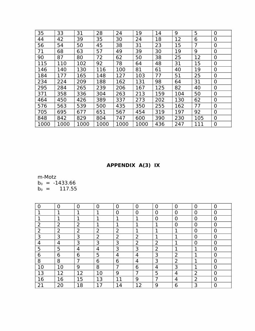
35 33 31 28 24 19 14 9 5 044 42 39 35 30 24 18 12 6 056 54 50 45 38 31 23 15 7 071 68 63 57 49 39 30 19 9 090 87 80 72 62 50 38 25 12 0115 110 102 92 78 64 48 31 15 0146 140 130 116 100 81 61 40 19 0184 177 165 148 127 103 77 51 25 0234 224 209 188 162 131 98 64 31 0295 284 265 239 206 167 125 82 40 0371 358 336 304 263 213 159 104 50 0464 450 426 389 337 273 202 130 62 0576 563 539 500 435 350 255 162 77 0705 695 677 651 567 454 319 197 92 0848 842 829 804 747 600 390 230 105 01000 1000 1000 1000 1000 1000 436 247 111 0
APPENDIX A(3) IX
m-Motzb0 = -1433.66b0 = 117.55
0 0 0 0 0 0 0 0 0 01 1 1 1 0 0 0 0 0 01 1 1 1 1 1 0 0 0 02 2 2 1 1 1 1 0 0 02 2 2 2 2 1 1 1 0 03 3 3 2 2 2 1 1 0 04 4 3 3 3 2 2 1 0 05 5 4 4 3 3 2 1 1 06 6 6 5 4 4 3 2 1 08 8 7 6 6 4 3 2 1 010 10 9 8 7 6 4 3 1 013 12 12 10 9 7 5 4 2 016 16 15 13 11 9 7 4 2 021 20 18 17 14 12 9 6 3 0

27 25 24 21 18 15 11 7 4 034 32 30 27 23 19 14 9 4 043 41 38 34 29 24 18 12 6 054 52 48 43 37 30 23 15 7 069 66 61 55 47 38 29 19 9 088 84 78 70 60 49 36 24 12 0112 107 99 89 76 62 46 30 15 0141 135 126 113 97 79 59 39 19 0179 172 160 143 123 100 75 49 24 0227 218 203 182 157 128 96 63 30 0286 275 257 232 200 163 122 80 39 0360 348 326 295 255 208 155 101 49 0452 437 412 376 327 266 198 128 62 0562 548 521 480 421 342 251 160 76 0693 680 655 614 548 446 317 196 92 0841 833 817 787 728 597 391 231 105 01000 1000 1000 1000 1000 1000 444 249 111 0
APPENDIX A(3) X
(Ignoring presence of singularity)
0 0 0 0 0 0 0 0 0 01 1 1 1 0 0 0 0 0 01 1 1 1 1 1 0 0 0 02 2 2 1 1 1 1 0 0 02 2 2 2 2 1 1 1 0 03 3 3 2 2 2 1 1 0 04 4 4 3 3 2 2 1 0 05 5 4 4 3 3 2 1 1 06 6 6 5 4 4 3 2 1 08 8 7 7 6 5 3 2 1 011 10 9 8 7 6 4 3 1 014 13 12 11 9 8 6 4 2 017 16 15 14 12 10 7 5 2 022 21 20 17 15 12 9 6 3 0

28 27 25 22 19 15 12 8 4 036 34 32 28 24 20 15 10 5 045 43 40 36 31 25 19 12 6 057 55 51 46 39 32 24 16 8 072 70 64 58 50 40 30 20 10 092 88 82 73 63 51 38 25 12 0117 112 104 93 80 65 49 32 16 0148 142 132 118 102 83 62 41 20 0187 179 167 150 130 106 80 52 26 0236 227 212 191 165 135 102 67 33 0297 286 268 243 210 172 130 86 42 0372 360 339 308 269 225 166 109 53 0464 451 427 392 348 284 214 139 67 0574 561 536 499 444 369 274 177 84 0703 691 670 634 577 486 352 220 103 0847 840 826 802 758 666 447 265 121 01000 1000 1000 1000 1000 1000 534 292 129 0
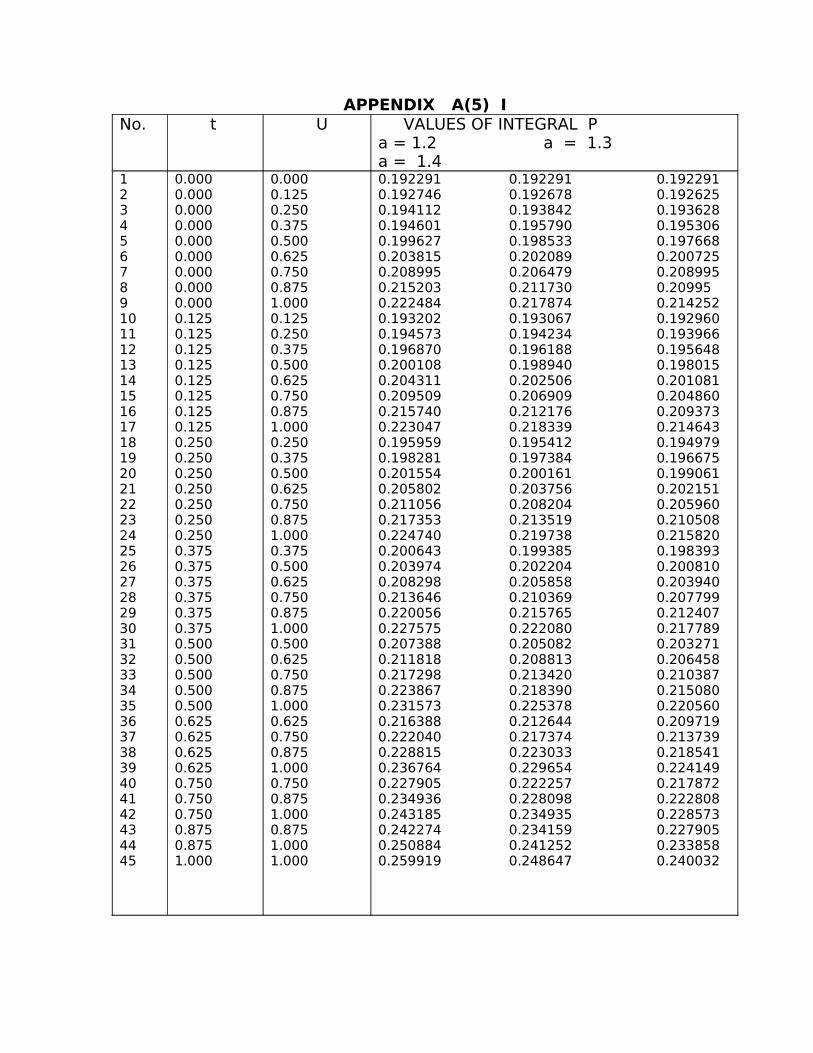
APPENDIX A(5) INo. t U VALUES OF INTEGRAL P
a = 1.2 a = 1.3 a = 1.4
123456789101112131415161718192021222324252627282930313233343536373839404142434445
0.0000.0000.0000.0000.0000.0000.0000.0000.0000.1250.1250.1250.1250.1250.1250.1250.1250.2500.2500.2500.2500.2500.2500.2500.3750.3750.3750.3750.3750.3750.5000.5000.5000.5000.5000.6250.6250.6250.6250.7500.7500.7500.8750.8751.000
0.0000.1250.2500.3750.5000.6250.7500.8751.0000.1250.2500.3750.5000.6250.7500.8751.0000.2500.3750.5000.6250.7500.8751.0000.3750.5000.6250.7500.8751.0000.5000.6250.7500.8751.0000.6250.7500.8751.0000.7500.8751.0000.8751.0001.000
0.192291 0.192291 0.1922910.192746 0.192678 0.1926250.194112 0.193842 0.1936280.194601 0.195790 0.1953060.199627 0.198533 0.1976680.203815 0.202089 0.2007250.208995 0.206479 0.2089950.215203 0.211730 0.209950.222484 0.217874 0.2142520.193202 0.193067 0.1929600.194573 0.194234 0.1939660.196870 0.196188 0.1956480.200108 0.198940 0.1980150.204311 0.202506 0.2010810.209509 0.206909 0.2048600.215740 0.212176 0.2093730.223047 0.218339 0.2146430.195959 0.195412 0.1949790.198281 0.197384 0.1966750.201554 0.200161 0.1990610.205802 0.203756 0.2021510.211056 0.208204 0.2059600.217353 0.213519 0.2105080.224740 0.219738 0.2158200.200643 0.199385 0.1983930.203974 0.202204 0.2008100.208298 0.205858 0.2039400.213646 0.210369 0.2077990.220056 0.215765 0.2124070.227575 0.222080 0.2177890.207388 0.205082 0.2032710.211818 0.208813 0.2064580.217298 0.213420 0.2103870.223867 0.218390 0.2150800.231573 0.225378 0.2205600.216388 0.212644 0.2097190.222040 0.217374 0.2137390.228815 0.223033 0.2185410.236764 0.229654 0.2241490.227905 0.222257 0.2178720.234936 0.228098 0.2228080.243185 0.234935 0.2285730.242274 0.234159 0.2279050.250884 0.241252 0.2338580.259919 0.248647 0.240032

APPENDIX A(5) II
No t U VALUES OF INTEGRAL Qa = 1.2 a = 1.3 a = 1.4
123456789101112131415161718192021222324252627282930313233343536373839404142434445
0.0000.0000.0000.0000.0000.0000.0000.0000.0000.1250.1250.1250.1250.1250.1250.1250.1250.2500.2500.2500.2500.2500.2500.2500.3750.3750.3750.3750.3750.3750.5000.5000.5000.5000.5000.6250.6250.6250.6250.7500.7500.7500.8750.8751.000
0.0000.1250.2500.3750.5000.6250.7500.8751.0000.1250.2500.3750.5000.6250.7500.8751.0000.2500.3750.5000.6250.7500.8751.0000.3750.5000.6250.7500.8751.0000.5000.6250.7500.8751.0000.6250.7500.8751.0000.7500.8751.0000.8751.0001.000
-1.000000 -1.000000 -1.000000-1.000603 -1.000514 -1.000443-1.002414 -1.002057 -1.001773-1.005441 -1.004634 -1.003994-1.009695 -1.008255 -1.007113-1.015194 -1.012930 -1.011138-1.021957 -1.018677 -1.016082-1.030013 -1.025513 -1.021957-1.039393 -1.033462 -1.028782-1.001207 -1.001028 -1.000887-1.003022 -1.002574 -1.002219-1.006055 -1.005156 -1.004443-1.010317 -1.008782 -1.007566-1.015826 -1.013466 -1.011598-1.022604 -1.019222 -1.016548-1.030675 -1.026070 -1.022432-1.040074 -1.034032 -1.029267-1.004848 -1.004127 -1.003557-1.007898 -1.006722 -1.005791-1.012186 -1.010367 -1.008928-1.017727 -1.015074 -1.012976-1.024544 -1.020859 -1.017948-1.032664 -1.027741 -1.023857-1.042119 -1.035744 -1.030722-1.010979 -1.009338 -1.008041-1.015308 -1.013013 -1.011200-1.02094 -1.017760 -1.015278-1.027788 -1.023593 -1.020285-1.035988 -1.030533 -1.026238-1.045536 -1.038604 -1.033152-1.019697 -1.016731 -1.014391-1.025369 -1.021533 -1.018510-1.032347 -1.027434 -1.023568-1.040660 -1.034456 -1.029580-1.050340 -1.042621 -1.022681-1.031140 -1.026406 -1.022681-1.038241 -1.032395 -1.027804-1.046699 -1.039522 -1.033894-1.056550 -1.047809 -1.040969-1.045492 -1.038493 -1.033008-1.054131 -1.045749 -1.039193-1.064192 -1.054188 -1.046379-1.062985 -1.053159 -1.045492-1.073297 -1.061778 -1.052811-1.083904 -1.070607 -1.060283

APPENDIX A(5) III
No T U VALUES OF INTEGRAL Qa = 1.2 a = 1.3 a = 1.4
123456789101112131415161718192021222324252627282930313233343536373839404142434445
0.0000.0000.0000.0000.0000.0000.0000.0000.0000.1250.1250.1250.1250.1250.1250.1250.1250.2500.2500.2500.2500.2500.2500.2500.3750.3750.3750.3750.3750.3750.5000.5000.5000.5000.5000.6250.6250.6250.6250.7500.7500.7500.8750.8751.000
0.0000.1250.2500.3750.5000.6250.7500.8751.0000.1250.2500.3750.5000.6250.7500.8751.0000.2500.3750.5000.6250.7500.8751.0000.3750.5000.6250.7500.8751.0000.5000.6250.7500.8751.0000.6250.7500.8751.0000.7500.8751.0000.8751.0001.000
-0.037511 0.175385 0.1753850.177848 0.177482 0.1771920.185352 0.183858 0.1826770.198264 0.194776 0.1920340.217227 0.210696 0.205601 0.243228 0.232315 0.2238840.277698 0.260624 0.2475940.322671 0.296998 0.2776980.381031 0.343340 0.3155050.180369 0.179622 0.1790310.188056 0.186129 0.1846130.201290 0.197277 0.1941390.220746 0.213545 0.2079590.247463 0.235660 0.2265980.282949 0.264657 0.2507910.329365 0.301982 0.2815500.389792 0.349639 0.3202380.196306 0.193041 0.1904930.210538 0.204898 0.2005380.231525 0.222241 0.2151360.260467 0.245887 0.2348660.299129 0.277018 0.2605530.350071 0.317297 0.2933310.417018 0.369062 0.3347540.226542 0.218004 0.2114900.250259 0.237240 0.2274450.283192 0.263599 0.2490910.327589 0.298527 0.2774060.386782 0.344098 0.3137580.465743 0.403278 0.3600430.278208 0.259362 0.2454450.317381 0.289880 0.2699850.370845 0.330679 0.3022960.443261 0.384508 0.3441180.541789 0.455399 0.3979120.365861 0.326442 0.2986500.433053 0.375862 0.3366970.525852 0.441980 0.3864500.655184 0.530564 0.4512550.520868 0.437744 0.3828040.644976 0.521917 0.4438340.822836 0.636987 0.5208680.817853 0.632751 0.5208681.073500 0.787799 0.6244601.457090 1.004266 0.761476

APPENDIX A(5) IV
No t U VALUES OF INTEGRAL Qa = 1.2 a = 1.3 a = 1.4
123456789101112131415161718192021222324252627282930313233343536373839404142434445
0.0000.0000.0000.0000.0000.0000.0000.0000.0000.1250.1250.1250.1250.1250.1250.1250.1250.2500.2500.2500.2500.2500.2500.2500.3750.3750.3750.3750.3750.3750.5000.5000.5000.5000.5000.6250.6250.6250.6250.7500.7500.7500.8750.8751.000
0.0000.1250.2500.3750.5000.6250.7500.8751.0000.1250.2500.3750.5000.6250.7500.8751.0000.2500.3750.5000.6250.7500.8751.0000.3750.5000.6250.7500.8751.0000.5000.6250.7500.8751.0000.6250.7500.8751.0000.7500.8751.0000.8751.0001.000
0.000000 0.000000 0.0000000.000000 0.000000 0.0000000.000000 0.000000 0.0000000.000001 0.000001 0.0000010.000003 0.000002 0.0000020.000007 0.000005 0.0000040.000018 0.000012 0.0000080.000046 0.000028 0.0000180.000116 0.000066 0.0000400.000000 0.000000 0.0000000.000000 0.000000 0.0000000.000002 0.000001 0.0000010.000004 0.000003 0.0000020.000011 0.000007 0.0000050.000027 0.000017 0.0000110.000067 0.000039 0.0000240.000169 0.000091 0.0000540.000001 0.000001 0.0000010.000004 0.000003 0.0000020.000007 0.000006 0.0000040.000024 0.000015 0.0000100.000059 0.000034 0.0000210.000150 0.000080 0.0000460.000382 0.000187 0.0001020.000009 0.000006 0.0000040.000023 0.000014 0.0000090.000058 0.000033 0.0000200.000147 0.000077 0.0000450.000374 0.000182 0.0000990.000967 0.000434 0.0002200.000058 0.000033 0.0000200.000146 0.000077 0.0000440.000373 0.000182 0.0000980.000964 0.000432 0.0002180.002527 0.001038 0.0004890.000373 0.000181 0.0000980.000963 0.000431 0.0002180.002526 0.001037 0.0004890.006752 0.002526 0.0011050.002526 0.001037 0.0004890.006752 0.002526 0.0011040.018536 0.006255 0.0025260.018536 0.006255 0.0025260.052851 0.015835 0.0058590.159811 0.041325 0.013845

APPENDIX A(5) V
No t u The kernel K(t,u)a = 1.2 a = 1.3 a = 1.4 a = 5/3
123456789101112131415161718192021222324252627282930313233343536373839404142434445
0.0000.0000.0000.0000.0000.0000.0000.0000.0000.1250.1250.1250.1250.1250.1250.1250.1250.2500.2500.2500.2500.2500.2500.2500.3750.3750.3750.3750.3750.3750.5000.5000.5000.5000.5000.6250.6250.6250.6250.7500.7500.7500.8750.8751.000
0.0000.1250.2500.3750.5000.6250.7500.8751.0000.1250.2500.3750.5000.6250.7500.8751.0000.2500.3750.5000.6250.7500.8751.0000.3750.5000.6250.7500.8751.0000.5000.6250.7500.8751.0000.6250.7500.8751.0000.7500.8751.0000.8751.0001.000
0.390012 0.426384 0.395928 0.3325790.463104 0.427318 0.396676 0.3330220.466712 0.430150 0.398939 0.3343600.472868 0.434964 0.402776 0.3366150.481800 0.441912 0.408291 0.3398320.493855 0.451219 0.415634 0.3440700.509534 0.463207 0.425022 0.3494140.529550 0.478320 0.436743 0.3559740.554911 0.497173 0.451192 0.3638920.464314 0.428267 0.397433 0.3334690.467986 0.431141 0.399726 0.3348190.474256 0.436031 0.403615 0.3370960.483361 0.443092 0.409205 0.3403430.495667 0.452559 0.416656 0.3446230.511702 0.464770 0.426189 0.3500220.532222 0.480190 0.438107 0.3566530.558308 0.499467 0.452819 0.3646640.471858 0.434148 0.402109 0.3362050.478479 0.439268 0.406155 0.3385460.488122 0.446678 0.411980 0.3418870.501209 0.456642 0.419760 0.3462950.518355 0.469542 0.429741 0.3518620.540460 0.485916 0.442265 0.3587120.568837 0.506522 0.457798 0.3670030.485725 0.444795 0.410474 0.3409960.496327 0.452819 0.416709 0.3444980.510811 0.463661 0.425065 0.3491260.529967 0.477789 0.435836 0.3549840.554970 0.495875 0.449432 0.3622120.587602 0.518888 0.466426 0.3709910.508413 0.461778 0.423560 0.3482360.525085 0.473966 0.432786 0.3531880.547426 0.489994 0.444756 0.3594760.577109 0.510760 0.459997 0.3672630.616786 0.537606 0.479257 0.3767690.545028 0.488111 0.443251 0.3585850.572227 0.506937 0.456947 0.3654670.609242 0.531725 0.474581 0.3740330.660361 0.564454 0.497191 0.3845550.606843 0.529842 0.473075 0.3731420.655479 0.560630 0.494140 0.3827580.725713 0.602429 0.521657 0.3946630.723314 0.600546 0.520151 0.3937730.827636 0.656768 0.554947 0.407542 0.999947 0.737258 0.600874 0.423831

APPENDIX A(5) VI Integral Equation INo t The function g(t)
a = 1.2 a = 1.3 a = 1.4 a = 5/3
123456789
0.0000.1250.2500.3750.5000.6250.7500.8751.000
2.06544 0.86815 1.73636 1.531562.07518 1.87072 1.73815 1.532382.08731 1.87856 1.74360 1.534932.10840 1.98204 1.75293 1.539242.13994 1.91189 1.76651 1.545432.18443 1.93926 1.78496 1.553652.25301 1.97595 1.80918 1.564152.33217 2.02478 1.84052 1.577222.45673 2.09044 1.88103 1.59328

Appendix A(5) VII
( ) [ ] ( )∫ −=++++=4
0 945
873212327
45
2 7
43210
x
x
vifh
fffffh
dxxf ξ
( ) [ ] ( )∫ −+++++=5
0 12096
275197550507519
288
5 7
543210
x
x
vifh
ffffffh
dxxf ξ
( ) [ ] ( )ξviiix
xf
hfffffff
hdxxf
1400
9941216272722721641
140 6543210
6
0
−++++++=∫
( ) [ ]∫ +++++++=7
076543210 751357713232989298913233577751
17280
7x
xffffffff
hdxxf
( )ξviiifh
518400
8183 9
−

APPENDIX A(5) VIII
Integral Equation II
u t A B C D E Kernel
0 0 0.000000
0.000000
0.000000
0.000000
0.000000
0.000000
.1 0 0.000000
0.000000
0.000000
0.000000
0.000000
0.000000
.1 .1
0.011702
- 0.000032
0.070042
0.056012
0.000266
- 0.957328
.1 .2
0.021953
- 0.000061
0.140084
0.113445
0.000591
- 1.915845
.1 .3
0.029300
- 0.000082
0.210127
0.173779
0.001045
- 2.876770
.1 .4
0.032280
- 0.000090
0.280169
0.238618
0.001730
- 3.841391
.1 .5
0.024150
- 0.000082
0.350211
0.309758
0.002807
-4.811098
.1 .6
0.019210
- 0.000054
0.420253
0.389273
0.004532
- 5.787446
.1 .7
0.000148
- 0.000001
0.490296
0.479622
0.007328
- 6.772218
.2 0 0.000000
- 0.000000
0.000000
0.000000
0.000000
0.000000
.2 .2
0.041002
- 0.000114
0.280169
0.229791
0.001311
- 3.834098
.2 .3
0.054233
- 0.000151
0.420253
0.352063
0.002321
- 5.757235
.2 .4
0.058715
- 0.000164
0.560338
0.483537
0.003852
- 7.687868
.2 .5
0.051490
- 0.000144
0.700422
0.627891
0.006262
- 9.628836
.2 .6
0.029563
- 0.000083
0.840507
0.789380
0.010136
-11.583316
.2 .7
0.010106
0.000028
0.980591
0.973053
0.016445
-13.550986
.3 0 0.000000
0.000000
0.000000
0.000000
0.000000
0.000000

.3 .3
0.070417
- 0.000196
0.630380
0.539549
0.004118
-8.645196
.3 .4
0.073444
- 0.000205
0.840507
0.741336
0.006853
-11.544681
.3 .5
0.058864
- 0.000164
1.050633
0.963159
0.011180
-14.460086
.3 .6
0.022174
- 0.000062
1.260760
1.211671
0.018176
-17.396376
.3 .7
- 0.041199
0.000115
1.470887
1.494786
0.029646
-20.359348
.4 0 0.000000
0.000000
0.000000
0.000000
0.000000
0.000000
.4 .4
0.070565
- 0.000197
1.120676
1.019171
0.011447
-15.417415
.4 .5
0.044127
- 0.000123
1.400845
1.325116
0.018766
-19.312221
.4 .6
- 0.011899
0.000033
1.681013
1.668565
0.030691
-23.236118
.4 .7
- 0.103632
0.000290
1.961183
2.060742
0.050431
-27.197445
.5 0 0.000000
0.000000
0.000000
0.000000
0.000000
0.000000
.5 .5
- 0.000197
0.000001
1.751056
1.724577
0.030957
-24.193446
.5 .6
- 0.081679
0.000229
2.101267
2.174187
0.051022
-29.113289
.5 .7
- 0.208005
0.000584
2.451478
2.689122
0.084655
-34.083333
.6 0 0.000000
0.000000
0.000000
0.000000
0.000000
0.000000
.6 .6
- 0.196304
0.000552
2.521521
2.745134
0.084922
-35.040661
.6 .7
- 0.365052
0.001027
2.941774
3.401441
0.142684
-41.034296
.7 0 0.00000 0.00000 0.00000 0.00000 0.00000 0.00000

0 0 0 0 0 0 .7 .
7- 0.585672
0.001651
3.432070
4.223835
0.243740
-48.073148

APPENDIX A(5) IX
Integral Equation II
No. g(t) c = 0.4 c = 0.5 c =0.6 c =0.7
1 g(0.0) 0 0 0 0
2 g(0.1) 0.03291 0.02039 0.01299 0.00892
3 g(0.2) 0.06574 0.03488 0.02586 0.01771
4 g(0.3) 0.09839 0.06075 0.03850 0.02624
5 g(0.4) 0.13078 0.08049 0.05076 0.03437
6 g(0.5) 0.09978 0.06250 0.04192
7 g(0.6) 0.07356 0.04872
8 g(0.7) 0.05452
APPENDIX A(5) X
Integral Equation IIFunction c = 0.4 c = 0.5 c = 0.6 c =0.7
( )∫c
dtttg0
0.00700 0.00829 0.00905

0.00946

• 'Ii
-13)J-\PP;~I,TJJI~~.
~ESTABLISH DBD002AOOKP4; SOLVES POISSON S EQUATION.; O/P 8;-+
begin librarf AO,A6,A7,A8,A9,A2700j commen Here the user is reqd to feed in the 5 procedures POISSON,DIRI,DESCRT,DERV,NEUM.
It could be done in any order;
procedure POISSON(x,y,r);value x,yj ~ x,y,rj r:~O;
procedure DIRI(x,y,z,d);value x,y,z; real x,y,dj integer Z;begin 1£ z=3 then d:=xxo+yXo;if z=2 then d:=y; end;
procedure DESCRT(X,Y,z,x,y);value X,Y,z; real X,y,X~y; integer z; begin if z=1 then begin x:=sqrt~-(YXY)); y:-sqrt(1.0-(XXX)); end·--' if z=2 then begin x:=O;y:=Yjend;
if z=3 then begin X·-X·y·-O"end·.. - , .- '--' endj
'" procedure DERV(x,y,z,a);value x,y,z;real x,y,aj inte,er z;
begin if z=1 then a:=3.141S~+arctan(-xJy; if z=2 then a:=3. 141S926S/2;if z~3 then a:=Oj
end· - -- ----'
procedure NEUM(x,y,z,d);value x,y,z; ~ x,y,d; integer z; begin if z=1 then,d:=yjend; .
real h,x,y,X,Y,RHS,D1,h1,h2,ml,m2,d,A,N1,N2; Integer f,w,ff,cols,i,nsor,ax,ay,k,pt,band,b,Z,acont,s,node,type,cut,totala,
sgn,zero,n,ub,natt,atype,q,a12,a21,a4 3,a34,a58,a85,a67,a76,a912,a129, a 1011, a 1110, sw, uw, bd,SP1, SO, SM1, SM2, UP1, Uo, TJi'v12, UM1, TO, ffail, sp, sm, b 1,b2, b3,b4,bS,b6,b7,b8,b9,b10;
~ integer arr~i] B,T,T>1[-2:2],a,P[O: 12];I array If [ 0: 1 ;
open(20); f:=forrnat([-nddddj]);find(100,[DG010002]); find(101,lDG010003]);interchange(100); interchan~e(101); - - . write text(o,llcclPART*Ilcc_J_]);
acont:=read(20); node:=read(20); b:=read(20);zero:=read(20);sgn:=read(20)·ax:=read(2U)jar:=read(20);h:=read(20);ub:=read(20);totala:=read(2C)5;cols:=read(20);ff:=read(2o);
a21:=2xax+ay; a 43:=4Xax+3xay; aS8:=5xax+8xay; a67:=6xax+7xay;a912:=9xax+12Xay; a1011:=10Xax+11xay;a12:=ax+2Xay; a34:=3xax+4Xay;a8S:=8xax+5xay; a76 :=7Xax+6xay; a129:=12Xax+9Xay; a1110:=11xax+l0Xay;sp:=(1+sgn)/2; sm:=(1-sgn)/2;
5 Tt' ] r P ,- err! rrtttn ". 'sa SI .. t mea - r 5 r' re. 1 't' ""en, ~ @ 1 WH Vi $" " 's Xl WtW t . 19 ¥. '''1tIot ",'''~~~~~>&;''';....c..>l;'''-''''~'''''''~h' _~,~ ..Jt t )0 h 1't2M'ftibhH' rt __
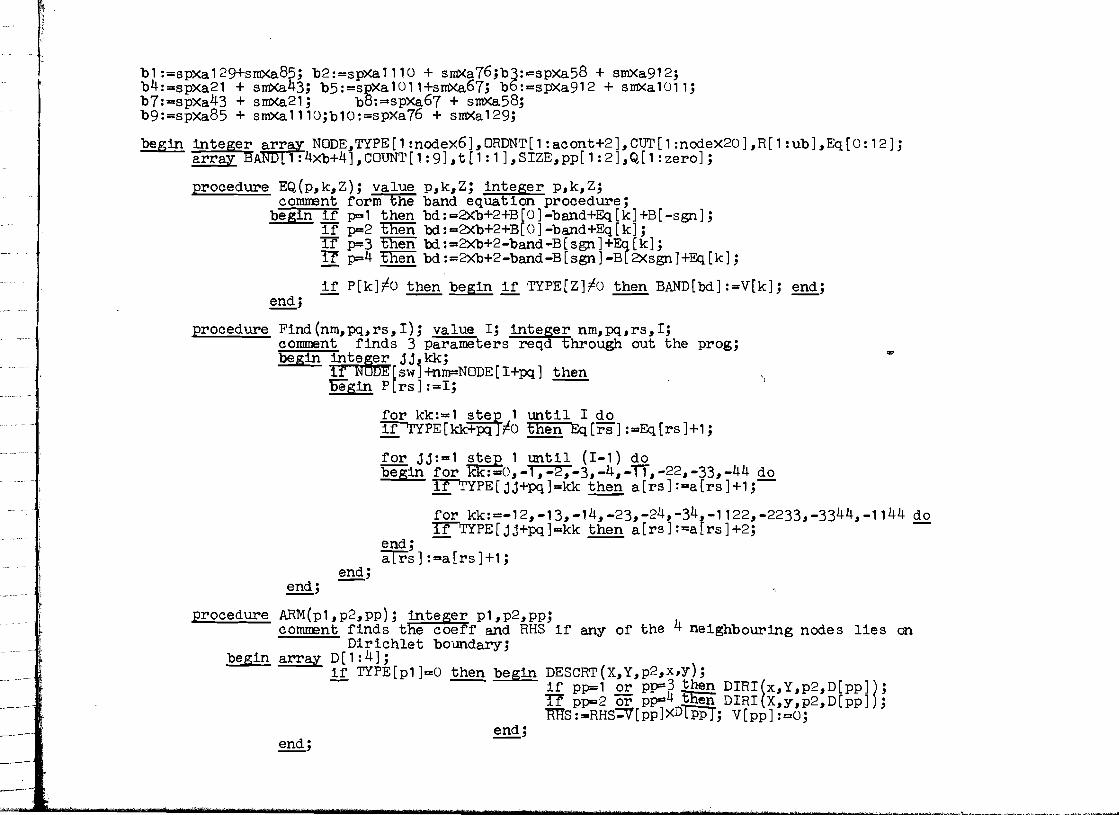
f abl:=spxa129+smxa85; b2: spXalll0 + sIDXa76;b3: a spxa58 + sIDXa912; b4:=spxa21 + srnxa43; b5:=s2xal0ll+srnxa67; b6:=sPXa912 + srnxal0l1; b7:=spxa43 + smxa21; b8:=spXa67 + smxa58; b9:=spXa85 + srnxalll0;bl0:=spxa76 + sMXa129;
begin integer NDf~ NODE,TYPE[1:nodex6],ORDNT[1:acont+2],CUT[1:nodeX20],R[1:ub],Eq[O:12]; array BA :4Xb+4],COUNT[1:9],t[1:1],S1ZE,pp[1:2],Q[1:zero];
procedure EQ(P,k,Z); value p,k,Z; integer p,k,Z;commmt form the band equation procedure;
begin if p=1 then bd:=2Xb+2+B[O]-band+Eq[k]+B[-sgn];if p=2 t'he'n bd:=2Xb+2+B[O]-band+Eq[k];If p=3 ~ bd.:=2Xb+2-band-B[sgn]+Eq[k];17 p=4 then bd:=2xb+2-band-B[sgn]-B[2Xsgn]+Eq[k];
if P[k]~O then begin if TYPE[Z]~O then BAND[bd] :=V[k]; end"--' end"--' procedure Find(nm,pq,rs,1); value I; integer nm,pq,rs,1;
comment finds 3 parameters reqd through out the prog; ....begin inte~er jj,kk;if Nl)E [sw ]+nm=NODE [ I +pq] then
"begin P[rs] :=1; -
for kk:=' ste! 1 until I do if TYPE[kk+pq ~o then Eq[rs] :=Eq[rs]+1;
for jj:=1 kaep 1 until (1-1) do begin for :=O,-1,-2,-3,-4,-TT,-22,-33,-44 do
rr-TYPE[jj+pq]=kk then a[rs]:=a[rs]+1;
for kk:=-12,-13,-'4,-23,-24,-34~-1'22,-2233,-3344,-1144do TI'"TYPE[jj+pq]=kk then a[rs]:=alrs]+2;
end; - - a[rs] :=a[rs]+1;
end"end; -'
procedure ARM(p1,p2,pp); integer pl,p2,pp; cornnent finds the coeff and RHS if any of the 4 neighbouring nodes lies on
Dirichlet boundary;---- -if begin array D[1:4];if TYPE[p1]=O then begin DESCRT(X,Y,p2,x,y); - - if pp=1 or pp==3 iiien D1R1(x,Y,p2,D[pp]);
if pp=2 or pp=4 ~ D1R1(X,y,p2,D[pp]); RRS:=RHS~[Pp]XDLPPJ; V[pp]:=O;
end"--' end;
X"¥ t _ tlt'ifrte 't t t 3 1" ,-"W' r $ t- rt t to t tnt tie,..,6(.' 1'" "'?til 4'",~""~..."_...._~"""":...... ....,,,,,.~,__~.-,."".£_ .•,~, ,_,~_,,_._"""'L'.''''.'''''j t t 3 •

procedure ZERO(t1,t2,t3,t4); integer t1,t2,t3,t4; ~~
if t3fO then ARM(aXX(sw-1)+ayx(SO+P[3]),axxCUT[UM1+a[3]]+ayXCUT[UO+a[3]],3);
if t2fO then ARM(aXX(SM2+P[2])+ayX(sw+1),axXCUT[UM2+a[2]]+ayXCUT[UM1+a[2]],2);
if t4fO then ARM(aXX(SO+P[4])+ayX(sw-1),axxCUT[UO+a[4]]+ayxCUT[UM1+a[4]],4);
if t1fO then ARM(axx(sw+1)+ayX(SM2+P[1]),aXXCUT[UM1+a[1]]+ayXCUT[UM2+a[1]],1); end;
real procedure tan(a); value a; real a; tan:=sin(a)/cos(a);
procedure STAR(n,m); integer n,rn; . comment cales coeffs for the 5-point star node; begIn real h1,h2,h3 t h4; real arr~ D[1:4];
~2:=h3:=hq:=h; ffail:= i);
if n)O then DESCRT(X,Y,CUT[uw],x,y); ...if n=l tEe:n begin h1 :=abS!X-Xj; D1R11X,Y,CUT[UW],D[1]j;end; if n=2 then begin h2:=abs y-Y ; DIRI X,y,CUT[uw],D[2] ;end; if n=3 then begrn h3:=abs x-X; DIRI x,Y,CUT[uw],D[3] ;entl; if n=4 then begin h4:=abs y-Y ; DIRI X,y,CUT[uw],D[4] ;end;
if rn)O then DESCRT(X,Y,CUT[uw+1],x,y); If m=2 then begin h2:=.abslY-YJ; D1R1lX,y,CUT[UW+1],D[2]j;end; if m=3 then begIn h3:=aos X-x; DIRI x,Y,CUT[uw+1],D[3] ;end; if m=4 then begin h4:=abs y-Y ; DIRI X,y,CUT[uw+1],D[4] ;end;
if h l)h .2!:. h2)h or h3)h or h4)h then goto FF;
V[O]:=-2XhXhx(~1/(h1Xh3)j + (1/(h2Xh3))J; .V[l]:=(2XhXh)! h1X(h1+h3 );V[2]:=(2XhXh 1(h2X(h2+h4));V[3]:=(2XhXh)/ h3X(h3+h1 );V[4]:=(2XhXh /(h4x(h4+h2));
if n)O then begin RHS:=RHS-V[n]XD[n]; V[n]:=O; end; If m)O then begin RHS:=RHS-V[m]xD[m]; V[m] :==0; end;
ZERO((l-n)X(l-m), (2-n)x(2-m),(3-n)x(3-m), (4-n)x(4-m));end'-'
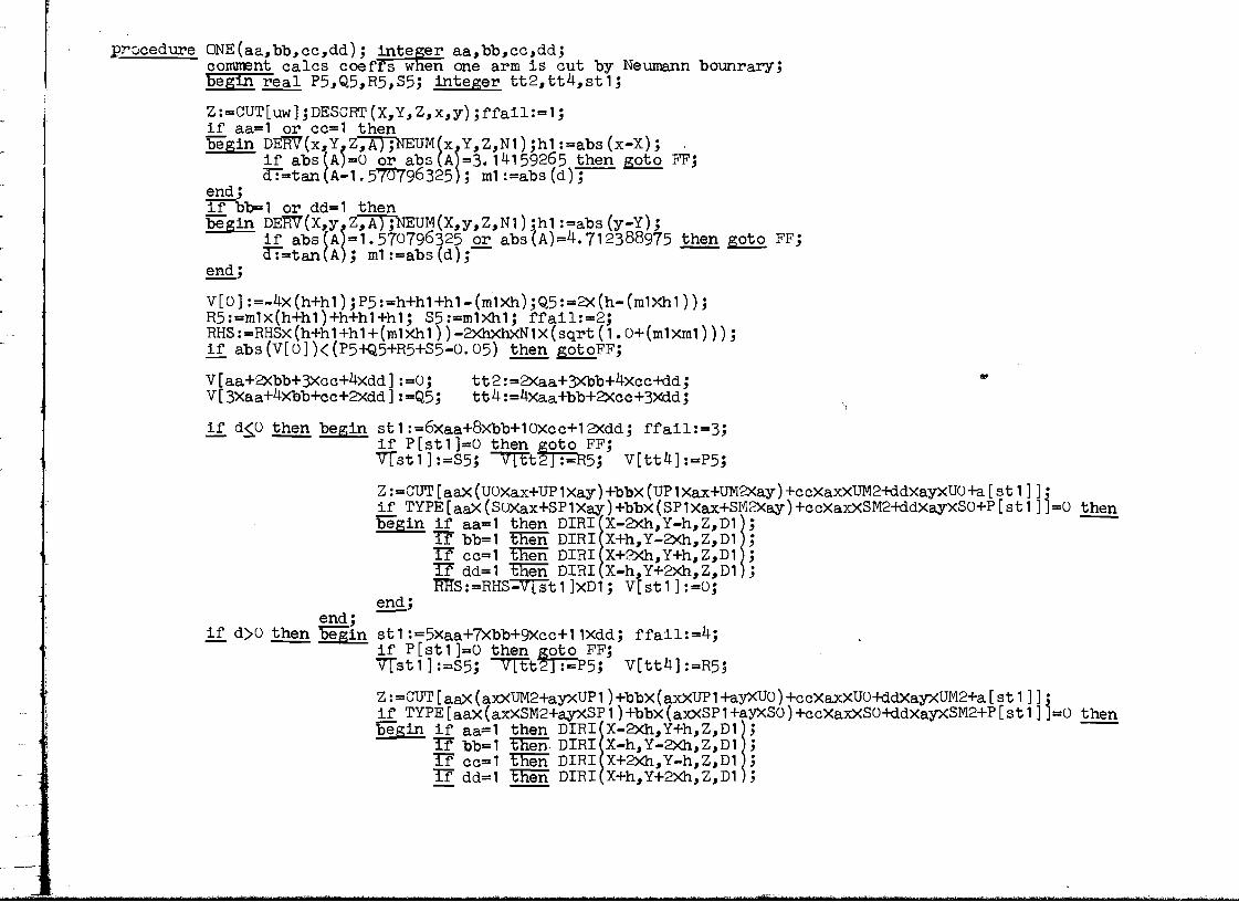
E~~cedure ONE(aa,bb,cc,dd); inte~er aa,bb,cc,dd; comment cales coeffs w en one arm is cut by Neumann bounrary;begin real P5,Q5,R5,S5; integer tt2,tt4,st1;
Z:=CUT[uw];DESCRT(X,y,Z,x,Y);ffail:=1; if aa=1 or cc=1 then begin DERV(X,Y~Z;AJ1NEUM(X~y,Z,N1);h1:=abS(x-X); .
if abs(A)=O or abs(A =3.14159265 then goto FF; a:=tan(A-1.51U796325; m1:=abs(d)-;-
end·--' if bb=1 or dd=1 then begin DE~(X,y~Z;AJTNEUM(X,y,Z,N1);h1:=abS(Y-Y);
if abs(A =1.570796325 or abs(A)=4.712388975 then goto FF; a:=tan(A; m1:=abs(d);-
end;
V[0]:=-4X(h+h1);P5:=h+h1+h1-(m1Xh);Q5:=2X(h-(m1Xh1));R5:=m1x(h+h1)+h+h1+h1; S5:=m1Xh1; ffail:=2; RHS:=RHSX(h+h1+h1+(m1Xh1))-2XhXhXN1x(sqrt(1.0+(m1Xm1)));if abs(V[0])«P5+Q5+R5+S5-0.05) then gotoFF;
...V[aa+2Xbb+3Xcc+4xdd]:=0; tt2:=2Xaa+3Xbb+4xcc+dd; V[3Xaa+4Xbb+cc+2Xdd]:-Q5; tt4:=4Xaa+bb+2Xcc+3Xdd;
if d~O ~ begin st1:=6Xaa+8Xbb+10Xcc+12Xdd; ffail:=3; if P[st1]=0 then ~]to FF;V[st1]:=S5; -vttt :=R5; V[tt4]:=P5;
Z:=CUT [aax (UOXax+UP 1Xay)+bbX (UP1Xax+UM2Xay)+ccxaxXUM2+ddxayXUO+a[st1]]·if TYPE[aaX(SOXax+SP1Xay)+bbX(SP1Xax+SM2Xay)+ccxaxXSM2+ddxayxSO+P[st1]j=0 then begin if aa=1 then DIRIIX-2Xh,Y-h,Z,D1j; ---
If bb=1 thin DIRI X+h,Y-2Xh,Z,D1 ; if cc=1 then DIRI X+2Xh,Y+h,Z,D1 ;If dd=1 tne:n DIRI X-h,Y+2Xh,Z,D1 ; RRS:=RHS~t1]XD1; V[st1]:=0;
end·-' end; if d)O ~ 'beiin st 1:=5Xaa+7Xbb+9Xcc+11Xdd; ffail:=4;
if P[st 1]=0 then ~FF; V[st1]:=S5; -v!tt21:=P5; V[tt4]:=R5;
Z:=CUT[aaX(axXUM2+ayxUP1)+bbX(axXUP1+ayXUO)+ccxaxxUO+ddxayxUM2+a[st1]]·if TYPE[aax(axXSM2+ayXSP1)+bbX(axXSP1+ayXSO)+ccXaxXSO+ddxayxSM2+P[st1]j=0 then begin if aa=1 then DIRIIX-2Xh,Y+h,Z,D1j; -
If bb=1 ~. DIRI X-h,Y-2Xh,Z,D1 ; If cc=1 thin DIRI X+2Xh,Y-h,Z,D1 ;If dd=1 then DIRI X+h,Y+2Xh,Z,D1 ;

I
\
RHS:=RHS-V[st1]XD1; V[st1]:=0; end'--' end;
ZERO(1-aa,1-bb;T-cc,1-dd);end'--'
procedure TWO(aa,bb,cc,dd); integer aa,bb,cc,dd; cornrrent cales coeffs when two arms are cut by Neumann bmmdary;begin real x1,x2,y1,y2,A1,A2, EX5,EX11,EX12,EX21,EX22,E1,E2,E3,E4;
Integer st1,st2,st3,st4,st5,st6,st7,st8,Z1,Z2; st 1:=5Xaa+7Xbb+9Xcc+1 1Xdd; st3:=3Xaa+4Xbb+cc+2Xdd; st2:=8xaa+10Xbb+12Xcc+6Xdd; st4:=4xaa+bb+2Xcc+3Xdd;
ffail:=5; if P[st1]=O and P[st2]=O then girO FF; ~:=CUT[uw];-nESCRT(X,y,zT;Xf,y ; Z2:=CUT[uw+1]; DESCRT(X,Y,Z2,x2,y2);
ffail:=6; if aa=1 or cc=1 then begin DE~(x1,Y~ZT;A1);NEUM(x1,y,Z1,N1);h1:=abs(x1-X);
if abs(A1)=0 or abs(A1)=3.141592b5 then goto FF; • mT:=tan(A1-1.'70796325);DERV(X,y2 Z2,A2);NEUM(X,y2,Z2,N2); h2:=abs(y2-Y); if abs(A2~=1.570796325 or abs(A2)=4.712388975 then goto FF;m2:=tan(A2); -- ---
end'-' if bb=1 or dd=1 then begin DERVTx,y1~Z"A1);NEUM(X,Y1,Z1,N1);h1:=abs(y1-Y);
if abs(A1)=1.570796325 or abs(A1)=4.712388975 then goto FF;mT:=tan(A1); -- - DERV(x2,Y~Z2,A2);NEUM(x2,y,Z2,N2);h2:=abs(x2-X);if abs(A2)=0 or abs(A2)=3.14159265 then goto FF;Iii2: =tan (A2- 1.1570796325) ; -
end'--' V[aa+2Xbb+3xcc+4xdd]:=V[2Xaa+3Xbb+4xcC+dd]:=0~ V[0]:=-2Xhx(h+h1+h2+(m1Xh2)-(m2Xh1)+(m1xm2Xh)); " RHS:=RHSX((h/2)X(hX(1.0+m1xm2)+(m1Xh1)-(m2Xh2)+(m1xm2X(h1+h2)))+(hX(h1+h2))+(h1Xh2X(2+m1-m2)))~ RHS:=RHS-hXhX((N1x(sqrt(1.0+(m1xm1)))X(h+h2+h2+m2Xh))+(N2X(sQrt(1.0+(m2Xm2)))X(h+h1+h1-(m1Xh)))); J
EX5:=(h1Xh2X(m1-m2))+((h/2)x((m1Xh1)-(m2Xh2)+(m1xm2X(h1+h2))));
E1:=lhXhx(1.0+(m1xm2j))+(2XhX(h2_(h1xm2)));E2:= m1xm2XhX(h1+h2) +(hX(m1Xh1-m2Xh2))+(2Xh1Xh2X(m1-m2));E3:= hXhX(1.0+(m1Xm2 ))+(2XhX(h1+m1Xh2));E4:= h1Xh2X(m1-m2))+((h/2)x((m1Xh1)-(m2Xh2)+(m1Xm2X(h1+h2)))); -)
EX11:=E1-E2;EX12:=E3+E4;
J

-,
if abs(V[O])«EX5+EX11+EX12-0,05) then goto Jl; "
Jl :
if P[stl]#O then begin V[s t 1]-:;;'EX5 ; v[s t 3] :=EX 1'; V[s t 4 ] :=EX12;
s t 5: =aaXSM2+bbXSP1+ccxSO+P [s t 1]; s t 7: =aaXSP 1+bbXS '+ddxSM2+P [s t 1] ;st6:=aaXUM2+bbXUP1+ccXUO+a[stl]; st8:=aaXUP1+bbXUO+ddXUM2+a[stl];Z:=CUT[axXst6+ayxst8], if TYPE[axXst5+ayXst7j=o then begin if' aa=1 then DIRI!X~'Y+h'Z'Dlj;
if b~1 then DIRI X-h,Y-2Xh,Z,Dl ; if cc=1 ~ DIRI X+2Xh,Y-h,Z,Dl ; if dd=1 then DIRI X+h~Y+2Xh,Z,Dl ; ~S:=RHS~tl]XD1; VLstl]:=O;
end'--' goto J2; end'-'
EX21:=El+E4; EX22:=E3-E2; ffail:=9; ...
..
-,
)
. ,
if abs(V[01)«EX21+EX22+EX5-0,05) then goto FF;
V[st2]:=EX5; V[st3]:=EX21; V[st4] :=EX22; .)
st5:=aaXSP1+bbXSM2+ddXSO+P[st2]; st7:=aaXSM2+ccXSO+ddXSP1+P[st2];st6:=aaXUP1+bbXUM2+ddXUO+a[st2]; st8:=aaxUM2+ccXUO+ddXUP1+a[st2];Z:=CUT[axXst6+ayXst8], if TYPE[axxst5+ayxst7j=o then oegin if aa=l then DIRI!X+h;7-2Xh,Z,Dlj;
If bb=1 tEen DIRI X+2Xh,Y+h,Z,Dl ; if cc=l then DIRI X-h,Y+2Xh,Z,Dl ; If dd=l tEen DIRI X-2Xh,Y-h,Z,Dl ; ]RS:=RHS~t2]XD1; V[st2]:=O;
end'--' J2: end'-'
ZERO((l-aa)X(l-dd),(l-aa)X(l-bb), (l-bb)X(l-cc), (l-cc)X( l-dd));
0'/
,)
~·,~ibl)&:r._:'.L'

i
"
T[sgn]:=M[sgn]:=T[2Xsgn]:=M[2xsgn]:=s:=node:=type:=pt:=cut:=acont:=q:=nsor:=O;
--~---- ....-;
READ: atype:=read(20); iif atypefl then natt:=O else natt:=-l;
ub:=read (20);for i :=1 ~ 1 until ub do
~l
1i[I"] : -read (20) ;
totala :=totala-l; 'i
if saO then goto G; i
COPY: if sgn=l then begin n:=O; for i:=l stiP 1 until R[2] do -,for k:=R[ 2X +1] step 1 untilR[2Xi+2] do n::;;n+l ;
if s=-l or s=-2 then '" begin if:s=-l then bd:=T[O]~
If s=-2 then bd:=T[-l J+T[O]+T[1 ]+T[,2]; -I
for i:=l Eyep 1 until bd do begin NOD n+l+bd-l]:=NODErbd+1-i];
TYPE[n+l+bd-i]:=TYPE[bd+l-i]; jend"--' end"--'
node :=type :=0; end"--'
G: n:=O;
for i:=l 2tiP 1 until R[2] do for k:=R[ x +1] step 1 untiI'R[2Xi+2] do begin node:=node+1; NODE[node]:=k; n:=n+1; end;
T[s]:=n; for i :=1 Rr~ 1 until n dobairn if R[2]+2+i]~0""""fhen ~t2 type:=type+l;
for k:=l stet 1 'lZlt'IT""n'[ ]+2+i] do OOiin type: = ype+l; TYPE [type] : == 1; end; n:=n+l-R[2XR[2]+2+i];
L: end"--'
-I
~\
1
TYPE[type]:=R[2XR[2]+2+i]; goto L; end;
-,
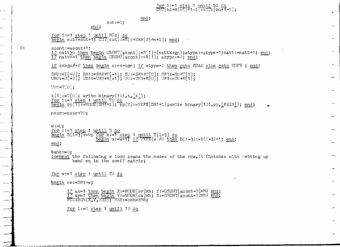
_
C:
_" ••,.~ ...__
for i:=' S~jP , until bd do CUT[bd+M[- +1-i1:=cUr[bd+T-i];
"-,
end; cut:=o;
",end;
for i:==1 step 1 until M[s] do begin cut:==cut+'j CUT[cut] :~[2+2XR[2]+n+i]; end; "-,
acont :==acont+1; if nattLo then begin ORDNT[acont]:=R[1]+(nattxsgn);atype:=atype-1;natt:=natt+1 j end; if natt=-l then begin ORDNT[acont]:=R[']; atype:==O; end;
if sxsgnf-2 then begin s :=s-sgn; if atype=O then goto READ else goto COPY; end;
SM2:=T[-2]; SM1:=SM2+T[-1]; SO:=SM1+T[0]; SP1:=SO+T[1]; -,UM2:==M[-2]; UH1:=Ul'12+M[-1]; UO:=UM1+M[O]; UP1:==UO+M[1];
TO :=T [0] ;
t [ 1] :==T [0].; wri te binary ( 10' , t, [t ] ) .; for i:=l srep 1 until TO do - Begin ppl' :=NODE(SM1+i];-Pp[2]:==TYPE[SM'+i];write binary(101,pp,lPA1Rl); end; ... nsor:=nsor+TO;
w:=O; for i:=1 st
JP 1 until 5 do -, begin B[i-3 :=0; for k:='-step 1 until T[i-3] do
begin w:=w+1; if TYPE[w]fO then B[i-3]:=B[i-3]+1; end'--' end'--' band:=O; comment the following w loop scans the nodes of the row,it finishes with "etting up
band eq in the coeff matrix;
for w:==1 step 1 until TO do
begin sw:=SM1+w;
ifax==' then begin X:=NODE[sw]Xh; Y:=ORDNT[acont-2]Xh; ~; -,if ay=l then ~Srin Y:=NODE[sw]Xh; X:=ORDNT[acont-2]Xh; end; mISSON("X;'Y';R" ; RHS:=hXhxRHS;
for i:=O step 1 until 12 do
~ .~<,""",-~~;-""~<"---,"'>.~.'-'-~ * d d 1 "Wet t t r t 1 $ me·;••!j,-,.i·,_~.~,~.~~._ .. __ _j," h t '@ H f t ( t t

begin Eg[i]:=a[i]:=P[i]:=O;VLi] :=0;
end'--' for i:=1 s~ep 1 until SM2 do begin Find -1,0,a129,i); Find(1,0,a1110,i); ~;
for i:=1 step 1 until T[-1] do '5e"gin Find (-2, SM2, a5S, i); Find (0, SM2, a21, i); Find (2, SI'I2,a 1C11, i); end;
for i:=1 step 1 until T[l] do begin Find(-2,SO,a67,i); Find(0,SO,a43,i); Find(2,SO,a9l2,i); end;
for i:=l step 1 until T[2] do begin PinctT=T,SP1,a76,i) ;Pind(1,SP1,a85,i); end;
if w)1 then ~ind(-1,SM1,a34,w-l);
Find(0,SM1,0,vl); uw:=UM1+a[0];
if wfTO then Find(1,SM1,a12,w+1); ... if TYPE[sw]=O then be~in q:=q+1; DIRI(X,Y,CUT[uw],Q[q]); goto Z~j end; if TYPE[sw]=-1-rhen S AR!1,0);if TYPE[sw]=-2 then STAR 2,0<; if TYPE[sw]=-3 then STAR 3,0<; if TYPE [sw ]=-4 then STAR 4,0 J • if TYPE[sw]=-12 then STAR 1,2 ; if TYPE[sw]=-13 then STAR 1,3 ; if TYPE[sw]=-14 then STAR 1,4 ; if TYPE[sw]=-23 then STAR 2,3 ; if TYPE[sw]=-24 then STAR 2,4 ; if TYPE[sw]=-34 then STAR 3~4 ; if TYPE[sw]=1 then-sTAR(O,O); if TYPE [sw ]=-1 1. thenONE (1,0,0,0) 1· if TYPE[sw]=-22 then ONElO,l,O,o ; ~'
if TYPE[sw]=-33 then ONE 0,0,1,0 ; if TYPE[sw]=-44 then ONE 0,0,0,1 ; if TYPE[sw]=-1122 then TWO!l,O,O,Oj;if TYPE[sw]=-2233 then TWO 0,1,0,0 ; if TYPE[sw]=-3344 then TWO 0,0,1,0 ; if TYPE[sw]=-1 14~ then T\m 0,0,0,1 ;
pt:=pt+1; band:=band+1' for i:=1 step 1 until 4Xb+3 do BAND[i] :=0: 1'11 :=BAND [2Xb+2] :=v[o]; if P[a12]fU then begin if TYPE[SM1+P[a12]]fO then BAND[[2Xb+3]:=V[a12] end; if P[a34]fo then begin if TYPE[Sfil1+P[a34]]fO -'then BAND 2Xb+1] :=V[a34] end;
-
I"•.-.........,_~....~ '& &9 '-) h iwe i bt' ¥' Me- 0 3 £ ., .+ l' +- .'2' $ t; t tnt It'" f? ' ...n

EQ 1,b1,sPXa129+smx(SP1+P[a85]))~ EQ 1,b2,spxa1"O + smx(SP1+P[a7bJ)); EQ 2,b3,spx SM2+P[a58]) + srnxlso+p[a912ll);EQ 2,b4,spx SM2+P[a21]) + sffiX sO+P[a43] ; EQ 2,b5,spx SM2+P[a1011])+srnx sO+P[a67] • EQ 3,b6,spx SO+p[a912j) + smx SM2+P[a1011j));EQ 3,b7,spx sO+P[a43] + Srnx!SM2+p[a21])); EQ 3,b8,spx sO+P[a67] + smx SM2+P[a58]));EQ 4J b9,spx SP1+P[a85 )+srnxP a1110]); . EQ 4,b10,spX(SP1+P[a76])+sffiXP[a129]);
,,BAND[4xb+4]:=RHS;
for i:=l Bifm 1 until (4Xb+4) do BmD [ i ] : = [i ]IN 1; " write binary ( 100, BAND, IBAND1) ;
•zz: end·--' ~.if sgn=1 then begin' for i:=4 st;! -1 until 1 do
- -- '""be~in T[i- :=T[i-3l; M[I=2] :=M[i-3] ;end; ~GG;
end; bd:=T[2]+T[1]+T[0]+~1]; ...
~'for i :==1 :EIe! 1 'lmtil bd do oegin NOD i :=NODE[T[-2]+r]; TYPE[i]:=TYPE[T[-2]+i]; end;
';:abd:=M[2]+M[1]+M[0]+M[-1]; for i:=1 ~[M 1 until bd do CUT"[i] :=C [-2]+1];
~
for i:=1 S~jP 1 until 4 do oegin T[i- :=T[i-2]; M[i-3]:=M[i-2]; ~;
type:=node:=T[-2]+T[-1]+T[0]+T[1];cut:=M[-2]+M[-1]+M[0]+M[1];
GG: if totala=-2 then ~otinF; If totala=-1 theneg totala:=-2;T[-sgn]:=M[-sgn]:=O; goto C; end;
.~
(" \:' if totala= 0 then begin if atype=O then begin totala:=-1; - .
- -- - - T[-2Xsgn] :=M[-2xsgn] :=0; if natt =-l ~ natt: =1; goto C; end·--' if atype)O ~ goto COPY;
end·--' if totala) 0 then begin if atype=O then gOtO READ; - -- If atype)O then ~ COPY; ~;
F: if cols)8 then cols:=8; COUNT [ 1] :=nsor; COUNT[2]:=acont-2;
....._, _<_,~<_.. "._, >_..~••.c.._.k'_""__','W.S,.,~~:i<""""" 1& M tid t t '&1 t 'fV t f - e '-'., 'Mt f s' 3 %6 ft' '-y t»W' fret; ,Z
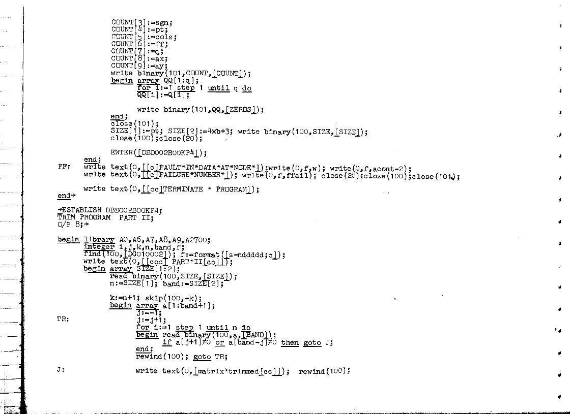
__ _ __ __ __
FF:
end-+
end; write write
write
COUNT[3]:=sgn;COUNT [4] :=pt; CClUN'I' [?] :=cols; COUNT[6]:=ff;COUNT [7] :=q; COUNT [8] :=ax; COUNT [9] :=a.yj write binary(101,COUNT,lCOUNT]);begin array QQ[1:q]; -
for i :=1 iyep 1 until q do mIT"i] :=Q[ ; -
write binary(101,QQ,lZEROS1);end" clo~e (101); SIZE[1]:=pt; SIZE[2]:=4Xb+3; write binary(100,SIZE,[ SIZE1);close(100);close(20); , -
ENTER(lDBD002BOOKP41);
text (0, [[c±FAULT*IN*DATA*AT*NoDE*l) "write (O,f w); write(0,f,acont-2); text(o,IIc FAILURE*NUMBER*l); writeto,f,ffail~; close(20);close(100);close(101~;
text (O,licclTERMINATE * PROGRAM1);
-+ESTABLISH DBDOO2B00KP4; TRIM PROGRAM PART II; Dip 8;-+
begin library AO,A6,A7,A8,A9,A2700; inte~er i,j,k,n,band,f; tind 100,[DG010002f); f:=format([s-nddddd;cl);write text (0, [[ccc PART*IIlcc]]J;begin array S'IZE[ 1:2]; -
read binary(100,SIZE,[SIZE]);n :=SIZE [1]; band :=SIZET2];
k:=n+1; skip(100,-k);begin arrat a[1:band+1];
j :-- ; TR: j :=j+1;
for i:=1 step 1 'lmtil n do begin read bin~(100,a,~AND]);
if a[j+1]10.2!: a[band-jT#O then goto J;end" rewind (100); goto TR;
J: write text(O,[matrix*trimmed[cc]]); rewind (100);- - -
,
.,
,
~
4
• ~
'4
4
'4
<I
-•
.. ,","·.·"'--c-"·'~·~''''"''.~.".·j_":h.,,. ""0" -_"","",",_."" .._(, ..:.o:...~~,~'='_'~. •'c..•~,,_'- .. ,.•"c.A,_.,....,,·_~, ......·............c·~._ ............, ...... _·. .~~ .•.•.._~..._.~·..~.~_"~_""~'_c.~ .•. ....~.>: .~~4". .•·_._,·,_ "~'~w.-.~~. ._~~.~~...•~ ,," ~, -,""",,;•.-.~u,-~ ~ ~...... ,.. M" C" Y' .. He w.....

------
----
• SIZE[l]:=n; SIZE[2] :=((band-j-j)+2);
•write text(O,[number*of*rows*is**]); write(U,f,n);write text(O,Thalf*band*width*is*T); write(0,f,SIZE[2]);- - .
•begin array A[l:n , (-SIZE[2]) :(SIZE[2])],B[1:n]; for i:=l step 1 until n do begin read binary{100,a,TBAND]); . ..
for k:=l stEt 1 until (band-j-j) do A[i,k-l-SIZ 2]] :=a[j+k]; - ..B[i]:=a[band+l];
end;
rewind(100); interchan$e(100); • write binarY~100,SIZE'LSIZE]); write binary 100,A,[A]T; write binary WO,B,IBI ; •
end; end;
end· • clo~e(100)· write text(o,[PART*II*OVER[cc]]); ENTER(lDBD002C~-KP41); --- '" •
end~
• ~ESTABLISH DBD002COOKP4; SOLVE PROGRAM PART III;
----_.._.. ----"• DIp 8;~ • begin library AO,A6,A7,A8,A9,A2700;
intefer i,j,k,n,w; • find 100, [DG010002]); write text(O,[[cc]PART**III[cc]]);
• begin array S[l :2]T read binar¥(100~,[~IZE]); n:~S[TT.~ w:=S[2]; begin array A[l:n , -w:wJ; read binary(100,A,lAl);
for j:=l step 1 until n do ..begin for i:= (if j)w then j-w+l else 2 ) step 1 ,until (if j(n-w then j+w else n) do
for k:=if j)i and j)w then j-welse if not J~i and i)w then i-weIse --- lstfp TU"ntil T'Ifj)i then i-l""'EDse j-n-do ---- - A[i,j-i] :=A i,j-i]-A[i,k-i]XA[k,j-k]; ---- -- • if A[j,O]=O.o then begin write text(0,ldiagonal*element*zero*TERMINATE*PROG1); goto Z;end;.
fo:: i:=j;-l [tep 1 unt~l (:f j(n-w then j+w ~ n) do• A[~,j-i] .=A i,j-i]/ALJ,O], ~... •
end'---' write text(o,llcltriangular*decomposition*overlcll); •
---~I ~

__
-- -- -- -- ----
begin array B[1:n]; read binary(100,B,lBl);
~or i:=2 step 1 until n do I
for j:=1 step 1 until (ir-i<w then i-1 else w) do B[i] :=B[iT=ATi,if i<w+1~en j-i else j-w-1]XBrTf i<w+1 then j else j+i-w-1]; .. for i:=n step -1 until 1 do
J begin A[ 1, -wJ :=0; - ..for j:=1 step 1 until (if i)n-w+l then n-i else w) do ATf, -w] :="A[T;"-w]+Ali, j ]Xb[i+j]; -- -
B[i] :=(B[i]-Al1,-w])/Ali,O]; end;
,write text(O,[[c]solution*obtained[c]]);rewind(100)jinterchange(1UO); -- write binarY(1oo,B,lRESULr~); .;
end"--' end; end' ..--' write text(U,[PART*III*OVER]); CIOSe!1UU); - ENTER [DBDU02D--KP41); ..
--------11 Z: close Too); •end-+
• ~ESTABLISH DBD002DOOKP4; OUTPUT PROGRAM PART IV; .o/p 8;~
begin library AO,A6,A7,A8,A9,A12,A2700; integer nsor,acont,sgn,k,i,j,pt,n,min,f,oldnode,newnode,oldrslt,newrslt,cols,zero, iii
oldzero,newzero,sum,ax,ay,v,m; real r; array COUNT[1:9]; open(70);find(100,lDG0100021); find(101,lDG0100031);write text(U,[[cc]PART **IV[cc]]);read binary ("oT, cTIUNT,lCOUNT] )-.- , nsor:=COUNT[1]; acont:=COUNTT21; sgn:=COUNT[3]; pt:=COUNT[4]; cols:=COUNT[S]; zero:=COUNT[7]; ,.' if COUNT[6]=1 then f:=format([s-nddddd.ddddd]); if COUNT[6]=o then f:=format(Ts-d.ddddddwfndT):ax:=COUNT [8]; ay:=COUNT[ 9]; - - , • n:=Oj rewind(101); .1 begin array ZEROS[1:zero],RESULT[1:pt],NODE,TYPE[1:nsor],T[1:acont ],Q[1:acont];
for i:=1 step 1 until acont do •b'e'gin T[rjY t [1 : 1]; read binary ( 101, t, [t]); i :=t[1]; -
begin array PAIR[1:2]; for j:=1 step 1 until t[1] do • begin n:=n+1~read binary(10~AIR,[PAIR]);
NODE[nJ:=PAIR[1]; TYPELn]:=PAIR[2T; end"--' end'---' end".~,
1t ,. • ;' h tr*$e1'ftMDr'·mhhrS'd rtf '1'1 £ ",:to He ,I, p' Wh11' .. :tM 'it- ~~""_' ""~,>......,~........-.....~."".."-:,"""",..;.,.\I""""""".,_,=~",,,,-.,,",",,.;;~,,,,-,-",~

~
rewind(1U1), read binary(1U1,ZEROS, [ZEROS1).; read binary(lUU,RESULT,[RESULTJ).; -~r (sgn=1 and aX=1) or Tsgn=-1-and ax=U) then "5'egin for i :=1 srel-1-Wltil (acont+2) do -
"begin k:=T i .; T[i] :-T[acont+1-iTI T[acont+1-iJ :=k;~;
~
~
'I,
,.'
-_. ----~~ -'
-~
14-·
..-.-._-~
•-----_.
NODE[nsor+1-iJ :=k; TYPE[nsor+1-iJ:=k;
do TT[iJ+2) do NODE[n+j-1j:=NODE[T[iJ+n-jJ;TYPE[n+j-1 J:=TYPE[T[iJ+n-jJ;
for i:=1 ~tDt 1 Wltil (nsor+2) do begin k:=lO [iJ; NODE[iJ:=NODETnsor+1-iJ;
k:=TYPE[i); TYPE[iJ:=TYPE[nsor+1-iJ; end"--' n :=1 ; for i:=1 step 1 Wltil acont begin for j: =1 N6Dr 1 until
begin k:= [n+j-1];k:=TYPE[n+j-1 J;
end"-'n:=n+T [ i);
NODE[T[iJ+n-jJ :=k; TYPE[T[iJ+n-jJ :=k;
end"-'n:=U; for i :=1 jte.p 1 until acont do begin Q[i :=0;
for j:=1 stj~ 1 until T[iJ do _ if TYPE[j+n 0 then Q[iJ:=QTiJ+1;n:=n+T [i] ; -
end· for'i:=l Ri§n 1 Wltil (pt+2) do begin r:= LT[i]; RESULT[iJ:=RESULT[pt+1-iJ; RESULT[pt+1-iJ:=r.; end; n:= 1; for i:=1 step 1 until acont do 'begin for j:=1 M;§P 1 until "{"Q:[iJ+2) do
begin r:= ULT[n+j-1J; RESULT[n+j-1J :=RESULT[Q[iJ+n-jJ; RESULT[Q[iJ+n-jJ:=r; end; n:-n+Q[iJ;
end"--' n:=O; for i:=1 step 1 until acont do begin Q[ i J :=0 ;
for j:=1 step 1 until T[iJ do if TYPE[j+nJ=o then Q[iJ:=QTi)+1;n:=n+T[iJ; ---
end"--' )for i:=1 Z~R§ 1 until (zero+2 do begin r:= S[iJ; ZEROS[iJ:=ZERDS[zero+1-iJ.; ZEROS[zero+1-iJ:=r; end; n :=1; for i:=1 step 1 Wltil acont do beg:in for j:=1 step 1 until "'(Q[iJ+2) do
begin r:=ZERTIS[n+j-1J; ZEROS[n+j=1):=ZEROS[Q[iJ+n-jJ; ZEROS[Q[iJ+n-jJ:=r; end; n:=n+Q[iJ;
end; end"--' sgn:=O;
~
~
~
.~
.~
~
~
.,
..
., •
•
•
•
•
• ~,,:";";:'A/lh.~·,..~_. _,.,.~~ __~, " .. t· _rtewe t 'XC' t t b¥ t t W t 4$'" 7 t en gantt t r r
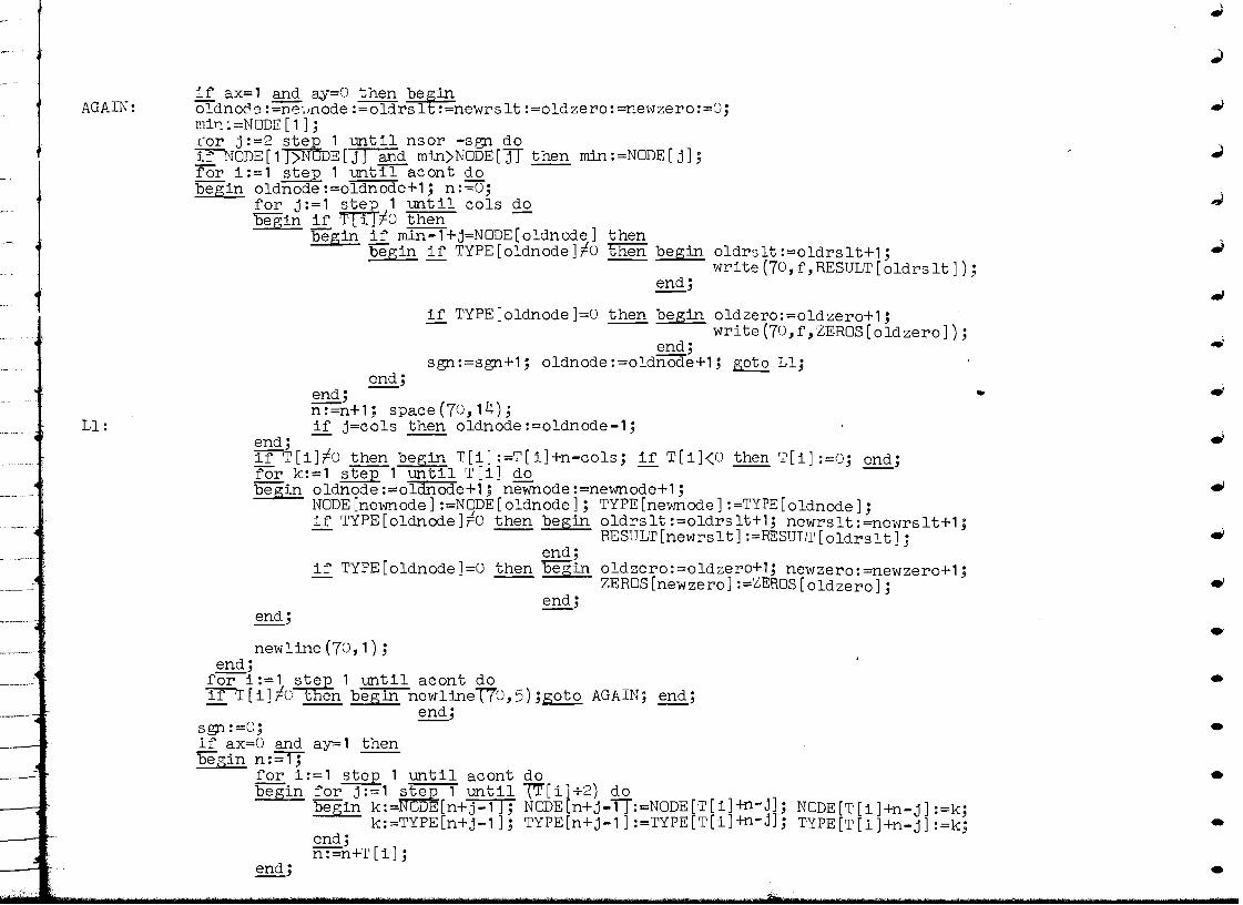
---
~
~
ifax=1 and ay=U then beginAGAIN: oldnoo8 :=ne',iDode :=oldrs 1 t :=newrs lt :=oldzero: =newzero :=U; ~
mi~ :=NoDE [1]; i'or j :=2 jte6 1 until nsor -sgn do IfNODE [1 )N DE [ j] and min)NoDE ["'IT then min: =NODE [ j] .; ~ for i :=1 step 1 untI'laeont do - 'b'egin oldnode :=oldnode+1.; n:;;o.;
,,)for j :=1 syeT1 until eols do begin if T i lU then
begin if min-1+j=NODE[oldnode] t~n
begin if TYPE[oldnode]lU then begin oldrslt:=oldrslt+1.; ~ --- write(7U,f,RESULT[oldrslt]);
end·
III
4' ---' ~
if TYPE[oldnode]=U then begin oldzero:=oldzero+1.; . -- ---- write(7U,f,ZERoS[oldzero]);
.,)end·---' sgn:=sgn+1.; oldnode:=oldnode+l; goto Ll; end;
•..end· ~~+1'; space (70,14) ;
Ll: if j=cols then oldnode:=oldnode-1';end; -- --- eJ ~[i]lU then begin T[i] :=T[i]+n-cols; if T[i]<U then T[i] :=0; end; for k:=1 step 1 until T[i] do
. .1>
.. begin oldnode:=oldnode+l; newnode:=newnode+1; eJ NoDE[newnode] :=NoDE[oldnode]; TYPE[newnode]:=TYPE[oldnode];
.....- ... if TYPE[oldnode]fU then begin oldrslt:=oldrslt+l; newrslt:=newrslt+1.; .;-- -- RESULT[newrslt]:=RESULT[oldrslt];
end·---' if TYPE[oldnode]=U then begin oldzero:=oldzero+l; newzero:=newzero+1; ,!I -- --- ZERoS[newzero]:=ZERoS[oldzero];
end· • •
--' .'end·---' newline(7U,1);
end·---' for i:=1 StfiP 1 until acont do •if T[i]lU v en begin newline1(U,5).;goto AGAIN; end;
end·_..-..---~ ---' sgn : =U; •ifax=O and ay=1 then begin n:=1; -
1
for i:=1 step 1 until acont do • begin for j:=1 Ngn~ 1 until ~[iJ+2) do
begin k:= [n+j-1]; NoDE[n+j-TT:=NoDE[T[i]+n-j]; NoDE[T[i]+n-j]:=k; k:=TYPE[n+j-1]; TYPE[n+j-1]:=TYPE[T[i]+n-j]; TYPE[T[i]+n-j] :=k; •
end; ~n+T[i] ;
end·--' • .tile.

I -,
n:=(); ~.
for i:=1 step 1 until aeont do 'begin Q[i] :=0 ;
for j:=1 stJ~ 1 until T[i] do .... if TYPE [j+n 0 then Q[ i] :=QTf] +1; n:=n+T[i]; -- .,
end'j --' n:=1; for i:=1 step 1 until aeont do .,'5'egin for j:=1 R;SfJ 1 until 1Q[i]+2) do
begin r:= ,J.:.< LT[n+j-1]; RESULT[n+j-1]:=RESULT[Q[i]+n-j]; RESULT[Q[i]+n-j]:=r; end; n:-n+Q[ i];
end' .. --' n:=O; fo.r i :=1 jt.eE 1 until aeont do '5'egin Q[i := ; ~
for j:=1 st P 1 until T[i] do Jf if TYPE[j+n =0 then Q[i]:=QTf]+1;J
~n:=n+T[i]; - end'--' n :=1;
~for i:=1 step 1 until aeont do ~
'5'egin for j :=1 ZiRB 1 until 1Q[ i] +2) do begin r:= S[n+j-1J; ZEROS[n+j-1]:=ZEROS[Q[i]+n-j]; ZEROS[Q[i]+n-j]:=r; end;
~n:=n+Q[i]; -- end'---' (for 1:=1 step 1 until aeont-sgn) do '5'eiin sum:=1; v:=sgn; - ~
JJ: n:=Oj for k:=1 ste11 until (if aeont-sgn<eols then acont-sgn else eols) do .,~n+T[k+sgn ; - -- --min :=NODE [1] ; for j :=2 ~tN8 1 until n do ~ODE[1J< DE[j] and min<NODE[j] then min:=NODE[j]; for j :=1 step 1 unt~(if aeont-sgn<eols ~ aeont-sgn else eols) do begin v:=v+1; if T[vJ=O then ~ LY1; .,
~
if m1n)NTIlJ'E[sum] then ~Y1; if m1n=NODE[sum] tnen oegin n:=m:=O;for k:=l step 1 until v-1 do n:=n+T[k]; .,
if TYPE [sum] f 0 then-- - begin for k:=1 J~ep 1 until n do
if TYPE[k 0 then m:-m+1; write(70,f,RE~[m+1]); -for k:=1 step 1 until (pt-m-1) do RESULT [m+k ] := RESULT l m+k+1]; pt:;;;Pt -1 ; -,end;
~YPE[sum]=O then begin for k:=1 jtep 1 until n do
~if TYPE[k =0 then m:-m+1;-writ e(70,f,ZEROSlm+1]); for k:=1 Jte~E1 until (zero-m- 1) do ZEttOS[m+k:= ROS[m+k+1]; .;
'1M ',., Hi"& ri&'" ">it", Itt me'i' Mlb'! bu" I;' \ 1'vms t' m ast ::100 rt~tkw'" nm' **-;-*~¢,'H stt t t'W jMt·t t

• • •
Ii t
t
• zero:=zero-1 ;
end; a. TTVT:=T[v]-1; if T[v]<U then T[v]:=G;newrslt:=newzero:=U; ---for k:=v step 1 until aeont do newrslt:=newrslt+T[k]; for k:=1 step 1 until (v-1) do newzero:=newzero+T[k]; • for k:=1 trep 1 until newrslt do begin NOD newzero+k]:=NODE[newzero+k+1];
TYPE[newzero+k]:=TYPE[newzero+k+1]; end; • sum:=sum+T[ v]; gotoLY2; -
end· a LY1 : s~~um+T[v]; spaee(7U,14);LY2: end·
newiine(70,1); v:=sgn; for k:=1 ,tep 1 until (if aeont-sgn<eols then aeont-sgn else eols) do if T[v+k] 0 then begin SUm:=1; goto JJ; end; ~~ sgn :=sgn+eols; newline (70, 5);
end"-' end"---'
• •
end-;.
end" elo~e(70);elose(100);elose(101);
... fIi
fIi
., ~
•
• • •

INDEX OF REFERENCES
1. Allen , D.N.de G(1954) Relaxation methods ,McGraw hill, New York , London.
2. Allen Fox, southwell (1946) Relaxation method applied to engineering problems. Phil.Trans. Roy. Soc. A,239, 501-537.
3. Appl. Math. Ser. U. S. Bur. Stand. 37(1954) Tables of functions and of zeros of functions, Government printing press, Washington.
4. Bickley, .G.(1948) Finite difference formulae for the square lattice, Quart . J. Mech. Appl. Maths. Vol. 1,35-42.
5. Collatz, L(1959) Numerical treatment of differential equations (Translated by P.G. Williams) Springer-Verlag, Berlin.
6. Forsythe and Wasow (1960) Finite difference methods for partial differential equations, John Wiley, New York.
7. Fox , L (1950) Numerical solution of elliptic differential equations when the boundary conditions involve a derivative , Phil. Trans. Roy. Soc. A , 242,345-378.
8. Fox, L(1962), [editor], Numerical solution of ordinary and partial differential equations-Oxford Summer School, Pergamon Press, London.
9. Greenspan, D(1965) Introductory numerical analysis of elliptic boundary value problems, Harper and Row , London.
10. Jeffreys, H and Jeffreys, B.S (1950) methods of mathematical physics, Cambridge University Press.
11. KDF 9 ALGOL manual, publication 1002, English Electric Leo computers Limited, Kidsgrove, Staffs.
12. Milne, W.E(1957) Numerical solution of differential equations, John Wiley , New York, London.
13. Motz, H (1946) the treatment of singularities of partial differential equations by relaxation methods; Quart. Appl. Math.4;372-377.

14. Scarborough, J.B.(1958) Numerical mathematical analysis; Baltimore : The Johns Hopkins Press; Oxford University Press.
15. Shaw, F.S(1950) An introduction to relaxation methods; Dover publications, New York.
16. Sneddon , I.N(1962a) Note on an electrified circular disk situated inside a coaxial infinite hollow cylinder; Proc. Camb. Phil. Soc.; 58;621-624.
17. Southwell, R.V.(1942) Proc. Roy. Soc. A, 180;367-396.
18. Srivastav, R.P(1963) Certain dual series relations and their applications; Ph.D. thesis, Glasgow University.
19. Varga, R.S(1957) Numerical solution of the two group diffusion equation in x-y geometry ; Inst. Radio Engrs.; Trans. Prof. Group Nuclear Science, Vol. NS-4,52-62.
20. Vishwanathan , R.V(1957) solution of Poisson’s equation by relaxation methods-normal gradient prescribed on curved boundaries ; Math. Tables Aids Compt. ,Vol.11. 67-78.
21. Wilson, S.B.L(1963) A difference method for the numerical solution of boundary –value problems; Ph.D. thesis, Glasgow University.
22. Woods, L.C(1953) The relaxation treatment of singular points in Poisson’s equation; Quart. J. Mech. 6.163-185.
