numerical solution of partial di erential equations using ... · contents contents 2 1 weak...

Numerical Solution of Partial Dierential Equations

Using Finite Element Methods

Aurélien Larcher

1

Contents

Contents 2

1 Weak formulation of elliptic PDEs 7

1.1 Historical perspective . . . . . . . . . . . . . . . . . . . . . . . . . 71.2 Weak solution to the Dirichlet problem . . . . . . . . . . . . . . . 7

1.2.1 Formal passage from classical solution to weak solution . . 81.2.2 Formal passage from weak solution to classical solution . . 91.2.3 About the boundary conditions . . . . . . . . . . . . . . . 9

1.3 Weak and variational formulations . . . . . . . . . . . . . . . . . 91.3.1 Functional setting . . . . . . . . . . . . . . . . . . . . . . 91.3.2 Determination of the spaces . . . . . . . . . . . . . . . . . 10

1.4 Abstract problem . . . . . . . . . . . . . . . . . . . . . . . . . . . 111.5 Well-posedness . . . . . . . . . . . . . . . . . . . . . . . . . . . . 121.6 Exercises . . . . . . . . . . . . . . . . . . . . . . . . . . . . . . . 14

2 Ritz and Galerkin for elliptic problems 17

2.1 Approximate problem . . . . . . . . . . . . . . . . . . . . . . . . 172.2 Ritz method for symmetric bilinear forms . . . . . . . . . . . . . 17

2.2.1 Variational formulation and minimization problem . . . . 172.2.2 Well-posedness . . . . . . . . . . . . . . . . . . . . . . . . 202.2.3 Convergence . . . . . . . . . . . . . . . . . . . . . . . . . 212.2.4 Method . . . . . . . . . . . . . . . . . . . . . . . . . . . . 23

2.3 Galerkin method . . . . . . . . . . . . . . . . . . . . . . . . . . . 232.3.1 Formulation . . . . . . . . . . . . . . . . . . . . . . . . . . 232.3.2 Convergence . . . . . . . . . . . . . . . . . . . . . . . . . 232.3.3 Method . . . . . . . . . . . . . . . . . . . . . . . . . . . . 25

2.4 Exercises . . . . . . . . . . . . . . . . . . . . . . . . . . . . . . . 26

3 Finite Element spaces 27

3.1 A preliminary example in one dimension of space . . . . . . . . . 283.1.1 Weak formulation . . . . . . . . . . . . . . . . . . . . . . 283.1.2 Galerkin method . . . . . . . . . . . . . . . . . . . . . . . 293.1.3 Construction of the discrete space . . . . . . . . . . . . . 303.1.4 Transport of Finite Element contributions . . . . . . . . . 323.1.5 Generalization of the methodology . . . . . . . . . . . . . 33

3.2 Admissible mesh . . . . . . . . . . . . . . . . . . . . . . . . . . . 34

2

CONTENTS 3

3.3 Denition of a Finite Element . . . . . . . . . . . . . . . . . . . . 343.4 Transport of the Finite Element . . . . . . . . . . . . . . . . . . . 373.5 Method . . . . . . . . . . . . . . . . . . . . . . . . . . . . . . . . 383.6 Exercises . . . . . . . . . . . . . . . . . . . . . . . . . . . . . . . 39

4 Simplicial Lagrange Finite Elements 41

4.1 Denitions . . . . . . . . . . . . . . . . . . . . . . . . . . . . . . . 414.2 Polynomial interpolation in one dimension . . . . . . . . . . . . . 424.3 Construction of the Finite Element space . . . . . . . . . . . . . 43

4.3.1 A nodal element . . . . . . . . . . . . . . . . . . . . . . . 434.3.2 Reference Finite Element . . . . . . . . . . . . . . . . . . 444.3.3 Lagrange Pk elements . . . . . . . . . . . . . . . . . . . . 44

4.4 Extension to multiple dimensions . . . . . . . . . . . . . . . . . . 454.4.1 Barycentric coordinates . . . . . . . . . . . . . . . . . . . 454.4.2 Ane transformation . . . . . . . . . . . . . . . . . . . . 47

4.5 Local equation for Lagrange P1 in one dimension . . . . . . . . . 494.6 Exercises . . . . . . . . . . . . . . . . . . . . . . . . . . . . . . . 51

A Denitions 53

A.1 Mapping . . . . . . . . . . . . . . . . . . . . . . . . . . . . . . . . 53A.2 Spaces . . . . . . . . . . . . . . . . . . . . . . . . . . . . . . . . . 53

B Duality 55

B.1 In nite dimension . . . . . . . . . . . . . . . . . . . . . . . . . . 55

C Function spaces 57

C.1 Banach and Hilbert spaces . . . . . . . . . . . . . . . . . . . . . . 57C.2 Spaces of continuous functions . . . . . . . . . . . . . . . . . . . . 58C.3 Lebesgue spaces . . . . . . . . . . . . . . . . . . . . . . . . . . . . 58C.4 HilbertSobolev spaces . . . . . . . . . . . . . . . . . . . . . . . . 58C.5 Sobolev spaces . . . . . . . . . . . . . . . . . . . . . . . . . . . . 58

D Inequalities 59

D.1 Useful inequalities in normed vector spaces . . . . . . . . . . . . 59

E Exercise solutions and hints 61

E.1 Chapter 1 . . . . . . . . . . . . . . . . . . . . . . . . . . . . . . . 62E.2 Chapter 2 . . . . . . . . . . . . . . . . . . . . . . . . . . . . . . . 64E.3 Chapter 3 . . . . . . . . . . . . . . . . . . . . . . . . . . . . . . . 65E.4 Chapter 4 . . . . . . . . . . . . . . . . . . . . . . . . . . . . . . . 66

Bibliography 67

4 CONTENTS

Introduction

This document is a collection of short lecture notes written for the course TheFinite Element Method (SF2561), at KTH, Royal Institute of Technology dur-ing Fall 2013, then updated for the course Numerical Solution of Partial Dif-ferential Equations Using Element Methods (TMA4220) at NTNU, during Fall2018. It is in not intended as a comprehensive and rigorous introduction toFinite Element Methods but rather an attempt for providing a self-consistentoverview in direction to students in Engineering without any prior knowlegdeof Numerical Analysis.

Content

The course goes through the basic theory of the Finite Element Method duringthe rst six lectures while the last three lectures are devoted to some applica-tions.

1. Introduction to PDEs, weak solution, variational formulation.

2. Ritz method for the approximation of solutions to elliptic PDEs

3. Galerkin method and well-posedness.

4. Construction of Finite Element approximation spaces.

5. Polynomial approximation and error analysis.

6. Time dependent problems.

7. Mesh generation and adaptive control.

8. Stabilized nite element methods.

9. Mixed problems.

The intent is to introduce the practicals aspects of the methods without hid-ing the mathematical issues but without necessarily exposing the details of theproof. There are indeed two side of the Finite Element Method: the Engineeringapproach and the Mathematical theory. Although any reasonable implementa-tion of a Finite Element Method is likely to compute an approximate solution,usually the real challenge is to understand the properties of the obtained solu-tion, which can be summarized in four main questions:

1. Well-posedness: Is the solution to the approximate problem unique?

2. Consistency : Is the solution to the approximate problem close to thecontinuous solution (or at least suciently in a sense to determine)?

3. Stability : Is the solution to the approximate problem stable with respectto data and well-behaved?

CONTENTS 5

4. Maximum principle, Physical properties: Does the discrete solution repro-duce features of the physical solution, like satisfying physical bounds orenergy/entropy inequalities?

Ultimately the goal of designing numerical scheme is to combine these propertiesto ensure the convergence of the method to the unique solution of the continuousproblem (if hopefully it exists) dened by the mathematical model. In a waythe main message of the course is that studying the mathematical propertiesof the continuous problem is a direction towards deriving discrete counterparts(usually in terms of inequalities) and ensuring that numerical algorithms possessgood properties.

Answering these questions requires some knowledge of elements of numer-ical analysis of PDEs which will be introduced throughout the document in adidactic manner. Nonetheless addressing some technical details is left to moreserious and comprehensive works referenced in the bibliography.

Literature

At KTH the historical textbook used mainly for the exercises is Computational

Dierential Equations [6] which covers many examples from Engineering butis mainly limited to Galerkin method and in particular continuous Lagrangeelements.

The two essential books in the list are Theory and Practice of Finite Ele-

ments [4] and The Mathematical Theory of Finite Element Methods [2]. Therst work provides an extensive coverage of Finite Elements from a theoreticalstandpoint (including non-conforming Galerkin, Petrov-Galerkin, DiscontinuousGalerkin) by expliciting the theoretical foundations and abstract framework inthe rst Part, then studying applications in the second Part and nally ad-dressing more concrete questions about the implementation of the methods ina third Part. The Appendices are also quite valuable as they provide a toolsetof results to be used for the numerical analysis of PDEs. The second work iswritten in a more theoretical fashion, providing to the Finite Element methodin the rst six Chapters which is suitable for a student with a good backgroundin Mathematics. Section 2 about Ritz's method is based on the lecture notes[5] and Section ?? on the description of the Stokes problem in [7].

Two books listed in the bibliography are not concerned with Numerical Anal-ysis but with the continuous setting. On the one hand, book Functional Anal-

ysis, Sobolev Spaces and Partial Dierential Equations [3] is an excellent intro-duction to Functional Analysis, but has a steep learning curve without a solidbackground in Analyis. On the other hand, Mathematical Tools for the Study

of the Incompressible NavierStokes Equations and Related Models [1], while re-taining all the diculties of analysis, oers a really didactic approach of PDEsfor uid problems in a clear and rigorous manner.

Chapter 1

Weak formulation of elliptic

Partial Dierential Equations

1.1 Historical perspective

The physics of phenomena encountered in engineering applications is often mod-elled under the form of a boundary and initial value problems. They consist ofrelations describing the evolution of physical quantities involving partial deriva-tives of physical quantities with respect to space and time, such relations arecalled Partial Dierential Equation (PDE). Problems involving only variationsin space are called boundary value problems as they involve the description of theconsidered physical quantities at the frontier of the physical domain. Equationsdescribing the evolution in time of physical quantities required the denitionof an initial condition in time, and are therefore called initial value problems.they consist of the coupling of an Ordinary Dierential Equation (ODE) in timewith a bounday value problem in space. The term Finite Element Method de-notes a family of approaches developed to compute an approximate solution toboundary and initial value problems.

The study of equations involving derivatives of the unknown has led to re-thinking the concept of derivation: from the idea of variation, then the studyof the Cauchy problem, nally to the generalization of the notion of derivativewith the Theory of Distributions. The main motivation is the existence of dis-continuous solutions produced by classes of PDEs or irregular data, for whichthe classical denition of a derivative is not suitable.

1.2 Weak solution to the Dirichlet problem

Let us consider the Poisson problem posed in a domain Ω, an open bounded sub-set of Rd, d ≥ 1 supplemented with homogeneous Dirichlet boundary conditions:

−∆u(x) = f(x), ∀ x ∈ Ω (1.1a)

u(x) = 0, ∀ x ∈ ∂Ω (1.1b)

7

8 CHAPTER 1. WEAK FORMULATION OF ELLIPTIC PDES

with f ∈ C0(Ω) and the Laplace operator,

∆ =d∑i=1

∂2

∂x2i

(1.2)

thus involving second order partial derivatives of the unknown u with respectto the space coordinates.

Denition 1.2.1 (Classical solution). A classical solution (or strong solution)of Problem (1.1) is a function u ∈ C2(Ω) satisfying relations (1.1a) and (1.1b).

Problem (1.1) can be reformulated so as to look for a solution in the distri-butional sense by testing the equation against smooth functions. Reformulatingthe problem amounts to relaxing the pointwise regularity (i.e. continuity) re-quired to ensure the existence of the classical derivative to the (weaker) existenceof the distributional derivative which regularity is to be interpreted in term interms of Lebesgue spaces: the obtained problem is a weak formulation and asolution to this problem (i.e. in the distributional sense) is called weak solu-

tion. Three properties of the weak formulation should be studied: rstly thata classical solution is a weak solution, secondly that such a weak solution isindeed a classical solution provided that it is regular enough, and thirdly thatthe well-posedness of this reformulated problem, i.e. existence and uniquenessof the solution, is ensured.

1.2.1 Formal passage from classical solution to weak solution

Let u ∈ C2(Ω) be a classical solution to (1.1) and let us test Equation (1.1a)against any smooth function ϕ ∈ C∞c (Ω):

−∫

Ω∆u(x)ϕ(x) dx =

∫Ωf(x)ϕ(x) dx

Since u ∈ C2(Ω), ∆u is well dened. Integrating by parts, the left-hand sidereads:

−∫

Ω∆u(x)ϕ(x) dx = −

∫∂Ω

∇u(x) ·nϕ(x) ds+

∫Ω∇u(x) ·∇ϕ(x) dx

For simplicity, we recall the one-dimensional case:

−∫ 1

0

∂2u

∂x2(x)ϕ(x)dx = −

[∂u

∂x(x)ϕ(x)

]1

0

+

∫ 1

0

∂u

∂x(x)

∂ϕ

∂x(x)dx

Since ϕ has compact support in Ω, it vanishes on the boundary ∂Ω, consequentlythe boundary integral is zero, thus the distributional formulation reads∫

Ω∇u(x) ·∇ϕ(x) dx =

∫Ωf(x)ϕ(x) dx , ∀ ϕ ∈ C∞c (Ω)

and we are led to look for a solution u belonging to a function space such thatthe previous relation makes sense.

1.3. WEAK AND VARIATIONAL FORMULATIONS 9

A weak formulation of Problem (1.1) consists in solving:∣∣∣∣∣∣∣Find u ∈ H, given f ∈ V ′, such that:∫

Ω∇u ·∇v dx =

∫Ωfv dx , ∀ v ∈ V

(1.3)

in which H and V are a function spaces yet to be dened, both satisfyingregularity contraints and for H boundary condition constraints. The choice ofthe solution space H and the test space V is described Section 1.3.

1.2.2 Formal passage from weak solution to classical solution

Provided that the weak solution to Problem (1.3) belongs to C2(Ω) then thesecond derivatives exist in the classical sense. Consequently the integration byparts can be performed the other way around and the weak solution is indeeda classical solution.

1.2.3 About the boundary conditions

Boundary condition Expression on ∂Ω Property

Dirichlet u = uD essential boundary conditionNeumann ∇u · n = 0 natural boundary condition

Essential boundary conditions are embedded in the function space, whilenatural boundary conditions appear in the weak formulation as linear forms.

1.3 Weak and variational formulations

1.3.1 Functional setting

HilbertSobolev spaces Hs (Section C.4) are a natural choice to measure func-tions involved in the weak formulations of PDEs as the existence of the integralsrelies on the fact that integrals of powers | · |p of u and weak derivatives Dαufor some 1 ≤ p < +∞ exist:

Hs(Ω) =u ∈ L2(Ω) : Dαu ∈ L2(Ω) , 1 ≤ α ≤ s

with the Lebesgue space of square integrable functions on Ω:

L2(Ω) =

u :

∫Ω|u(x)|2 dx < +∞

endowed with its natural scalar product

( u , v ) L2(Ω) =

∫Ωu v dx

Since Problem (1.3) involves rst order derivatives according to relation,∫Ω∇u ·∇v dx =

∫Ωfv dx


then we should consider a solution in H1(Ω).

H1(Ω) =u ∈ L2(Ω) : Du ∈ L2(Ω)

with the weak derivative Du i.e. a function of L2(Ω) which identies withthe classical derivative (if it exists) almost everywhere, and endowed with thenorm,

‖ · ‖H1(Ω) = ( · , · )1/2H1(Ω)

dened from the scalar product,

( u , v ) H1(Ω) =

∫Ωu v dx+

∫Ω∇u ·∇v dx

Moreover, the solution should satisfy the boundary condition of the strongform of the PDE problem. According to Section 1.2.3 the homogeneous Dirichletcondition is embedded in the function space of the solution: u vanishing on theboundary ∂Ω yields that we should seek u in H1

0(Ω).

1.3.2 Determination of the spaces

We will now establish that any weak solution lives in H10(Ω) and that the

natural space for test functions is the same space.

Choice of test space

In order to give sense to the solution in a HilbertSobolev space we need tochoose the test function ϕ itself in the same kind of space. Indeed C∞c (Ω) isnot equipped with a topology which allows us to work properly. If we choseϕ ∈ H1

0(Ω) then by denition, we can construct a sequence (ϕn)n∈N of functionsin C∞c (Ω) converging in H1

0(Ω) to ϕ, i.e.

‖ϕn − ϕ‖H1(Ω) → 0, as n→ +∞

For the sake of completeness, we show that we can pass to the limit in theformulation, term by term for any partial derivative:∫

Ω∂iu ∂iϕ

n →∫

Ω∂iu ∂iϕ

as ∂iϕn Diϕ in L2(Ω), which denotes the weak convergence i.e. tested onfunctions of the dual space (which, in case of L2(Ω), is L2(Ω) itself).∫

Ωf ϕn →

∫Ωf ϕ

as ϕn → ϕ in L2(Ω). Consequently the weak formulation is satised if ϕ ∈H1

0(Ω).

1.4. ABSTRACT PROBLEM 11

Choice of solution space

The determination of the function space is guided,

• rstly, by the regularity of the solution: if u is a classical solution then itbelongs to C2(Ω) which involves that u ∈ L2(Ω) and ∂iu ∈ L2(Ω), thusu ∈ H1(Ω),

• secondly by the boundary conditions: the space should satisfy the Dirichletboundary condition on ∂Ω. This constraint is satised thanks to thefollowing trace theorem for the solution to the Dirichlet problem: sinceKer(γ) = H1

0(Ω), we conclude u ∈ H10(Ω).

Lemma 1.3.1 (Trace Theorem). Let Ω be a bounded open subset of Rd with

piecewise C1 boundary, then there exists a linear application γ : H1(Ω) →L2(∂Ω) continous on H1(Ω) such that γ(u) = 0⇒ u ∈ Ker(γ).

The regularity of the solution itself depends on the nature of the dierentialoperators involved in the problem (e.g. up to which order should be derivativescontrolled?), but also on the data of the problem: regularity of the domain andright-hand side.

The weak formulation of Problem (1.1) reads then:∣∣∣∣∣∣∣Find u ∈ H1

0(Ω), such that:∫Ω∇u ·∇v dx =

∫Ωfv dx , ∀ v ∈ H1

0(Ω)(1.5)

1.4 Abstract problem

The study of mathematical properties of PDE problems is usually performed ona general formulation called abstract problem which reads in our case:∣∣∣∣∣∣

Find u ∈ V , such that:

a(u, v) = L(v) , ∀ v ∈ V(1.6)

with a( · , · ) a continuous bilinear form on V × V and L( · ) a continuous linearform on V .

Proposition 1.4.1 (Continuity). A bilinear form a( · , · ) is continuous on V ×W if there exists a positive constant real number M such that

a(v, w) ≤M‖v‖V ‖w‖W , ∀ (v, w) ∈ V ×W

For example, in the previous section for Problem (1.5), the bilinear formreads

a : V × V → R

(u, v) 7→∫

Ω∇u ·∇v dx


and the linear form,L : V → R

v 7→∫

Ωf v dx

The continuity of these two forms comes directly from that they are respec-tively the inner-product in H1

0(Ω), and the L2 inner-product with f ∈ L2(Ω):the CauchySchwarz inequality gives directly a continuous control of the imageof the forms by the norms of its arguments.

Denition 1.4.2 (Topological dual space). The topological dual space V ′ ofa normed vector space V is the vector space of continuous linear forms on Vequipped with the norm:

‖f‖V ′ = supx∈V,x 6=0

|f(x)|‖x‖V

In the following chapters, we consider the case of elliptic PDEs, like thePoisson problem, for which the bilinear form a( · , · ) is coercive.

Proposition 1.4.3 (Coercivity). A bilinear form is said coercive in V if there

exists a positive constant real number α such that for any v ∈ V

a(v, v) ≥ α‖v‖2V

This property is also know as V ellipticity.

1.5 Well-posedness

In the usual sense, a problem is well-posed if it admits a unique solution whichis bounded in the V -norm by the data: forcing term, boundary conditions,which are independent on the solution and appear at the right-hand side ofthe equation. In this particular case of the Poisson problem the bilinear forma( · , · ) is the natural scalar product in H1

0(Ω), thus it denes a norm in H10(Ω)

(but only a seminorm in H1(Ω) due to the lack of deniteness, not a norm !).

Theorem 1.5.1 (RieszFréchet). Let H be a Hilbert space and H ′ its topologicaldual, ∀ Φ ∈ H ′, there exists a unique representant u ∈ H such that for any

v ∈ H,

Φ(v) = ( u , v )H

and furthermore ‖u‖H = ‖Φ‖H′

This result ensures directly the existence and uniqueness of a weak solutionas soon as a( · , · ) is a scalar product and L is continuous for ‖ · ‖a. If thebilinear form a( · , · ) is not symmetric then Theorem 1.5.1 (RieszFréchet) doesnot apply.

Theorem 1.5.2 (LaxMilgram). Let H be a Hilbert space. Provided that a( · , · )is a coercive continuous bilinear form on H×H and L( · ) is a continuous linear

form on H, Problem (1.6) admits a unique solution u ∈ H.

1.5. WELL-POSEDNESS 13

Now that we have derived a variational problem for which there exists aunique solution with V innite dimensional (i.e. for any point x ∈ Ω), we needto construct an approximate problem which is also well-posed.


1.6 Exercises

Exercises for this section cover some preliminary notions introduced for the weakformulation of PDEs.

Exercise 1.6.1 (Based on Exercise 4 from [8]).Answer the following questions.

(a) Discuss whether the set S =v ∈ C∞c ((0, 1)) : v(1

2) = 1is a vector space.

(b) For V = H10((0, 1)), show that L(v) =

∫ 10 xv dx denes a linear func-

tional. Recall the denition of the topological dual V ′ and show that L iscontinuous for x ∈ V .

(c) For V ≡ R discuss whether ( u , v )V = |u||v| is an inner-product in V .(d) Does |u|H1(Ω) = ‖∇u‖L2(Ω), Ω ∈ R2 dene a norm in H1(Ω)? Explain why.

(e) Assess whether the function f(x) = x3/4 an element of the followingspaces: L2((0, 1)), H1((0, 1)), H2((0, 1)).

(f) For v = e−10x and Ω = (0, 1), is the relation |u|H1(Ω) = |u|H2(Ω) satised?

Exercise 1.6.2.

Let us consider the following problem posed on the domain Ω = (0, 1), with κa real coecient, and f ∈ L2(Ω):∣∣∣∣∣∣∣

Find u ∈ H10(Ω) such that:∫

Ωκ∂u

∂xv dx+

∫Ω

∂u

∂x

∂v

∂xdx+

∫Ωuv dx =

∫Ωfv dx, v ∈ H1

0(Ω)(1.7)

(a) Formulate the strong problem corresponding to weak formulation (1.7).(b) Discuss the existence and uniqueness of the solution to Problem (1.7).

Exercise 1.6.3.

Let us consider the biharmonic equation posed on the domain Ω = (0, 1):

∆2u(x) = f(x), ∀ x ∈ Ω (1.8a)

with f ∈ L2(Ω), and satisfying the boundary condition on ∂Ω

u(x) = u′(x) = 0, ∀ x ∈ ∂Ω (1.8b)

(a) For f ≡ 1 give a solution to Problem (1.8).(b) Derive a weak formulation (WF) of Problem (1.8).(c) Specify the solution space and the test space.(d) Show that there exists a unique solution u to (WF) belonging to the chosen

solution space.

Exercise 1.6.4.

Let us consider the Helmoltz equation posed on the domain Ω = (0, 1), given κa real coecient:

− u′′(x) + κu(x) = f(x), ∀ x ∈ Ω (1.9a)

with f ∈ L2(Ω),u(x) = 0, ∀ x ∈ ∂Ω (1.9b)

1.6. EXERCISES 15

(a) Derive a weak formulation (WF) of Problem (1.9).(b) Specify the solution and test spaces.(c) What is the nature of the bilinear form for κ = 1?(d) Prove that the problem is well-posed for κ = 0 and κ > 0.(e) Comment on the diculty posed by the case κ < 0.(f) The boundary condition is now given by:

u(0)− u′(0) = 0, u′(1) = −1 (1.10)

Derive a weak formulation for the Problem (4.2a)(1.10) and show that itadmits a unique solution. To prove the coercivity the following relationcan be used:

v(1) = v(x) +

∫ 1

xv′(t) dt

Chapter 2

Ritz and Galerkin methods for

elliptic problems

In Section 1. we have reformulated the Dirichlet problem to seek weak solutionsand we showed its well-posedness. The problem being innite dimensional, it isnot computable.

Question: Can we construct an approximation to Problem (1.1) which isalso well-posed?

2.1 Approximate problem

In the previous section we showed how a classical PDE problem such as Problem(1.1) can be reformulated as a weak problem. The abstract problem for this classof PDE reads then: ∣∣∣∣∣∣

Find u ∈ V , such that:

a(u, v) = L(v) , ∀ v ∈ V(2.1)

with a( · , · ) a coercive continuous bilinear form on V ×V and L( · ) a continuouslinear form on V .

Since in the case of the Poisson problem the bilinear form is continuous,coercive and symmetric, the well-posedness follows directly from RieszFréchetrepresentation Theorem. If the bilinear form is still coercive but not symmetricthen we will see that the well-posedness is proven by the LaxMilgram Theorem.

But for the moment, let us focus on the symmetric case: we want now toconstruct an approximate solution un to the Problem (2.1) then prove that thesolution to the obtained approximate problem exists and is unique.

2.2 Ritz method for symmetric bilinear forms

2.2.1 Variational formulation and minimization problem

The idea behing the Ritz method is to replace the solution space V (which isinnite dimensional) by a nite dimensional subspace Vn ⊂ V , dim(Vn) = n.

17

18 CHAPTER 2. RITZ AND GALERKIN FOR ELLIPTIC PROBLEMS

Problem (2.2) is the approximate weak problem by the Ritz method:∣∣∣∣∣∣∣Find un ∈ Vn, Vn ⊂ V , such that:

a(un, vn) = L(vn) , ∀ vn ∈ Vn(2.2)

with a( · , · ) a coercive symmetric continuous bilinear form on V × V and L( · )a continuous linear form on V .

Provided that the bilinear form is symmetric, Problem (2.3) is the equivalentapproximate variational problem under minimization form:∣∣∣∣∣∣∣∣∣∣

Find un ∈ Vn, Vn ⊂ V , such that:

J(un) ≤ J(vn) ,∀ vn ∈ Vn

with J(vn) =1

2a(vn, vn)− L(vn)

(2.3)

Proposition 2.2.1 (Equivalence of weak and variational formulations). Prob-lem 2.2 and 2.3 are equivalent.

Before moving to the well-posedness of the approximate variational prob-lem some denitions are introduced to caracterize the solution of mimimizationproblems, then the equivalence of formulations for the Poisson problem withhomogeneous Dirichlet boundary conditions in one dimension of space is givenas example.

Denition 2.2.2 (Directional derivative). Let V be a Hilbert space, for anyu ∈ V the relation:

J ′(u;w) = limε→0

1

ε

(J(u+ εw)− J(u)

)(2.4)

denes J ′(·; ·) : V × V → R derivative of the functional J at u in the directionw.

Denition 2.2.3 (Fréchet derivative). Let V be a Hilbert space, J is Fréchet-derivable at u if:

J(u+ v) = J(u) + Lu(v) + ε(v)‖v‖V (2.5)

with Lu a continuous linear form on V and ε(v)→ 0 as v → 0.

Proposition 2.2.4 (Optimality conditions). Let V be a Hilbert space and J a

twice Fréchet-derivable functional, u0 ∈ V is solution to

infv∈V

J(v) (2.6)

if the following conditions are satised:

1. J ′(u0) = 0 (Euler condition).

2.2. RITZ METHOD FOR SYMMETRIC BILINEAR FORMS 19

2. ( J ′′(u)w , w ) ≥ 0 (Legendre condition).

Both conditions can be interpreted in terms of the simpler case of real func-tions: the rst one requires that the rst derivative cancels so that u0 is anextremum, while the second condition is a convexity argument. Moreover, a suf-cient condition is given by ( J ′′(u)w , w ) ≥ 0 for any u in a neighbourhood of u0

(strong Legendre condition). The coercivity of the bilinear form a(·, ·) is an evenstronger condition equivalent to: ∃α > 0 such that ( J ′′(u)w , w ) ≥ α(w,w).

Example 2.2.5. Equivalence of weak and variational formulations for the Dirich-let problem posed on Ω = (0, 1). Let us derive the expression of J ′(u;w) denedby (2.4) given ε > 0 and w ∈ V .

First let us verify that if u solves the minimization problem then it solvesthe corresponding weak problem.

J(u+ εw) =1

2

∫Ω

[(u+ εw)′

]2dx−

∫Ωf(u+ εw) dx

=1

2

∫Ω

[(u′)2 + 2εu′w′ + ε2(v′)2

]dx−

∫Ωfu dx− ε

∫Ωfw dx

= J(u) + ε

[∫Ωu′w′ dx−

∫Ωfw dx

]+

1

2ε2

∫Ω

(w′)2 dx

Writing the derivative gives,

limε→0

1

ε

(J(u+ εw)− J(u)

)= lim

ε→0


∫Ωfw dx+

1

2ε|w|H1

0

]so that the Euler condition holds if for any w ∈ V = H1

0(Ω)

J ′(u;w) =

∫Ωu′w′ dx−

∫Ωfw dx = 0

In this case the functional J is Fréchet-derivable as Lu is linear.

Secondly, the other way around considering that the weak formulation holdsfor the test function εw ∈ V then in the relation

J(u+ εw) = J(u) + ε


∫Ωfw dx

]+

1

2ε2

∫Ω

(w′)2 dx

the second term of the right-hand side cancels, and the third term is non-negative, then

J(u+ εw) ≥ J(u)

so that u is solution to the minimization problem.

The same result holds for the continuous problem in V and the approxima-tion in Vn since only requirement is to work in a Hilbert space. Actually thefollowing result for the Dirichlet problem is due to Stampacchia which charac-terizes the solution to the weak problem in term of minimization.


Theorem 2.2.6 (Stampacchia). Let a(·, ·) be a bilinear coercive continuous

form on H a Hilbert space, and K be a convex closed non-empty subset of H.

Given φ ∈ H ′, ∃!u ∈ K such that

a( u , v − u ) ≥ 〈 φ , v − u 〉H′,H , ∀ v ∈ K

and if a is symmetric then

u = argminv∈K

1

2a( v , v )− 〈 φ , v 〉H′,H

The solution can be seen as satisfying a minimization of energy, also called

Dirichlet principle.

2.2.2 Well-posedness

Theorem 2.2.7 (Well-posedness). Let V be a Hilbert space and Vn a nite di-

mensional subspace of V , dim(Vn) = n, Problem (2.2) admits a unique solution

un.

Proof. Given that the weak formulation diers only by introducting nite di-mensional subspaces the proof could conclude directly with the LaxMilgramTheorem. Instead we show that there exists a unique solution to the equivalentminimisation problem (2.3) by explicitly constructing an approximation un ∈ Vndecomposed uniquely on a basis (ϕ1, · · · , ϕn) of Vn:

un =n∑j=1

uj ϕj

In practice this basis is not any basis but the one constructed to dene theapproximation space Vn: to one chosen approximation space will correspond onecarefully constructed basis. In so doing, the constructive approach paves theway to the Finite Element Method and is thus chosen as a prequel to establishingthe Galerkin method.

Writing the minimisation functional for un reads:

J(un) =1

2a(un, un)− L(un)

=1

2a(

n∑j=1

ujϕj ,n∑i=1

uiϕi)− L(n∑j=1

uiϕi)

=1

2

n∑i=1

n∑j=1

a(ujϕj , uiϕi)−n∑j=1

L(uiϕi)

=1

2

n∑i=1

n∑j=1

ujuia(ϕj , ϕi)−n∑j=1

uiL(ϕi)

Collecting the entries by index i, the functional can be rewritten underalgebraic form:

J(u) =1

2u

TAu− u

Tb

2.2. RITZ METHOD FOR SYMMETRIC BILINEAR FORMS 21

where u is the vector of algebraic unknowns also calleddegrees of freedom

uT

= (u1, . . . , un)

and A, b are respectively the stiness matrix and the load vector:

Aij = a(ϕj , ϕi),bi = L(ϕi)

Proposition 2.2.8 (Convexity of a quadratic form).

J(u) = uT

Ku− uT

G + F

is a strictly convex quadratic functional i K symmetric positive denite non-

singular.

As a consequence to Proposition 2.2.8 J is a strictly convex quadratic form,then there exists a unique u ∈ Rn : J(u) ≤ J(v),∀ v ∈ Rn, which in turnsproves the existence and uniqueness of un ∈ Vn.

The minimum is achieved with u satisfying Au = b which corresponds tothe Euler condition J ′(un) = 0

The general setting for Galerkin methods will be to construct approximatesolutions of the form:

un =

n∑j=1

ujϕj (2.8)

where uj1≤j≤n is a family of real numbers and B = (ϕ1, . . . , ϕn) a basis of Vn.Since Vn is nite dimensional, there exist a unique decomposition (2.8) on thebasis. This basis can be chosen in a way that seems natural so that in practicewe will construct a unique basis for a given type of space Vn and which willdene the approximation properties (the basis itself is not unique but we needto choose one that possesses good properties).

2.2.3 Convergence

The question in this section is: considering a sequence of discrete solutions(un)n∈N, with each un belonging to Vn, can we prove that un → u in V as n→∞? The ingredients are similar to the Lax principle: stability and consistencyimplies convergence.

Lemma 2.2.9 (Estimate in the energy norm). Let V be a Hilbert space and Vna nite dimensional subspace of V . We denote by u ∈ V , un ∈ Vn respectively

the solution to Problem (2.1) and the solution to approximate Problem (2.2).Let us dene the energy norm ‖ · ‖a = a( · , · )1/2, then the following inequality

holds:

‖u− un‖a ≤ ‖u− vn‖a , ∀ vn ∈ Vn


Proof. Using the coercivity and the continuity of the bilinear form, we have:

α‖u‖2V ≤ ‖u‖2a ≤M‖u‖2V

then ‖u‖a is norm equivalent to ‖u‖V , thus (V, ‖ · ‖a) is a Hilbert space.

a(u− PVn u, vn) = 0 ,∀ vn ∈ Vn

by denition of PVn as the orthogonal projection of u onto Vn with respect tothe scalar product dened by the bilinear form a.

‖u− un‖2a = a(u− un, u− vn) + a(u− un, vn − un) , ∀ vn ∈ Vn

Since the second term of the right-hand side cancels due to the consistency ofthe approximation, we deduce un = PVn u, then un minimizes the distance fromu to Vn:

‖u− un‖2a ≤ ‖u− vn‖2a , ∀ vn ∈ Vn

which means that the error estimate is optimal in the energy norm.

Lemma 2.2.10 (Céa's Lemma). Let V be a Hilbert space and Vn a nite dimen-

sional subspace of V . we denote by u ∈ V , un ∈ Vn respectively the solution to

Problem (2.1) and the solution to approximate Problem (2.2) , then the following

inequality holds:

‖u− un‖V ≤√M

α‖u− vn‖V , ∀ vn ∈ Vn

with M > 0 the continuity constant and α > 0 the coercivity constant.

Proof. Using the coercivity and continuity of the bilinear form, we bound theleft-hand side of the estimate (2.2.9) from below and its right-hand side fromabove:

α‖u− un‖2V ≤M‖u− vn‖2V ∀ vn ∈ Vn

Consequently:

‖u− un‖V ≤√M


Lemma (2.2.10) gives a control on the discretisation error en = u−un whichis quasi-optimal in the V -norm (i.e. bound multiplied by a constant).

Lemma 2.2.11 (Stability). Any solution un ∈ Vn to Problem (2.2) satises:

‖un‖V ≤‖L‖V ′α

2.3. GALERKIN METHOD 23

Proof. Direct using the coercivity and the dual norm. First, the inequality

α‖un‖2V ≤ a(un, un) = L(un)

holds for some α > 0, and secondly by denition of the dual norm,

‖L‖V ′ = supv∈V,v 6=0

L(v)

‖v‖V

so thatα‖un‖V ≤ ‖L‖V ′

2.2.4 Method

Algorithm 2.2.12 (Ritz method). The following procedure applies:

1. Chose an approximation space Vn

2. Construct a basis B = (ϕ1, . . . , ϕn)

3. Assemble stiness matrix A and load vector b

4. Solve Au = b as a minimisation problem

2.3 Galerkin method

2.3.1 Formulation

We use a similar approach as for the Ritz method, except that the abstractproblem does not require the symmetry of the bilinear form. Therefore wecannot endow V with a norm dened from the scalar product based on a( · , · ).

Problem (2.9) is the approximate weak problem by the Galerkin method:∣∣∣∣∣∣∣Find un ∈ Vn, Vn ⊂ V , such that:

a(un, vn) = L(vn) ,∀ vn ∈ Vn(2.9)

with a( · , · ) a coercive continuous bilinear form on V ×V and L( · ) a continuouslinear form on V .

2.3.2 Convergence

The following property is merely a consequence of the consistency, as the con-tinuous solution u is solution to the discrete problem (i.e. the bilinear formis the same), but it is quite useful to derive error estimates. Consequently,whenever needed we will refer to the following proposition:


Proposition 2.3.1 (Galerkin orthogonality). Let u ∈ V , un ∈ Vn respectively

the solution to Problem (2.1) and the solution to approximate Problem (2.9),then:

a( u− un, vn ) = 0 , ∀ vn ∈ Vn

Proof. Direct consequence of the consistency of the method. The approximateproblem

a( un, vn ) = L(vn) , ∀ vn ∈ Vn (2.10)

is obtained by replacing V by a nite dimensional space Vn but the relation

a( u, v ) = L(v) , ∀ v ∈ V (2.11)

from the weak formulation is otherwise the same: a(·, ·) and L(·) are unchanged.Since Vn ⊂ V , it is possible to choose v ∈ Vn in Equation (2.11), then

a( un, vn ) = a( u, vn ) , ∀ vn ∈ Vn (2.12)

which gives directly the orthogonality property.

Lemma 2.3.2 (Consistency). Let V be a Hilbert space and Vn a nite dimen-

sional subspace of V . we denote by u ∈ V , un ∈ Vn respectively the solution to

Problem (2.1) and the solution to approximate Problem (2.9), then the following

inequality holds:

‖u− un‖V ≤M


with M > 0 the continuity constant and α > 0 the coercivity constant.

Proof. Using the coercivity:

α‖u− un‖2V ≤ a(u− un, u− un)

≤ a(u− un, u− vn) + a(u− un, vn − un)︸︷︷︸0

≤ a(u− un, u− vn)

≤ M‖u− un‖V ‖u− vn‖V

‖u− un‖V ≤ M

α‖u− vn‖V

The only dierence with the symmetric case is that the constant is squareddue to the loss of the symmetry.

2.3. GALERKIN METHOD 25

2.3.3 Method

Algorithm 2.3.3 (Galerkin method). The following procedure applies:

1. Chose an approximation space Vn

2. Construct a basis B = (ϕ1, . . . , ϕn)

3. Assemble stiness matrix A and load vector b

4. Solve Au = b


2.4 Exercises

Exercise 2.4.1.

Given an abstract weak problem posed in a Hilbert space V :∣∣∣∣∣∣∣Find u ∈ V , V , such that:

a(u, v) = L(v) ,∀ v ∈ V

and a minimization problem∣∣∣∣∣∣∣∣∣∣Find u ∈ V , V , such that:

J(u) ≤ J(v) ,∀ v ∈ V

with J(v) =1

2a(v, v)− L(v)

(a) Show the equivalence of the formulations when a is bilinear symmetricpositive denite and L linear.

(b) Show that if V = Rn the minimization problem can be recast into a striclyconvex quadratic form J(u) = 1

2uT

Au − uTb and the unique solution

satises Au = b.

Exercise 2.4.2.

Let us consider the Poisson problem posed on the domain Ω = (0, 1):

− u′′(x) = f(x), ∀ x ∈ Ω (2.13a)


u(x) = 0, ∀ x ∈ ∂Ω (2.13b)

(a) For f ≡ 1 give a solution to Problem (2.13).(b) Find the weak formulation (WF) of Problem (2.13) and specify the func-

tion spaces.(c) Is this problem well-posed?(d) Justify that it is possible to reformulate this problem into a minimization

problem?(e) Derive the minimisation functional J(u).(f) Let w1 = a1 sin(πx). Find the value of the amplitude a1 minimizes J(w1).

How does a1 compare with the maximum of the exact solution u?(g) Show that J(w1) > J(u) and interpret.(h) Let φi = sin

((2i − 1)πx

), i ∈ N. Verify that these function are innitely

dierentiable and satisfy φi(0) = φi(1) = 0. Compute coecients

aij =

∫ 1

0φ′i(x)φ′j(x) dx , bi =

∫ 1

0φi(x) dx

(i) Given a nite dimensional space Vn = spanφi1≤i≤n, express the linearsystem obtained by the Galerkin method and give the solution.

Chapter 3

Finite Element spaces

In the previous lectures we have studied the properties of coercive problems inan abstract setting and described Ritz and Galerkin methods for the approx-imation of the solution to a PDE, respectively in the case of symmetric andnon-symmetric bilinear forms.

The abstract setting reads:∣∣∣∣∣∣Find uh ∈ Vh ⊂ H such that:

a(uh, vh) = L(vh) , ∀ vh ∈ Vh

such that:

• Vh is a nite dimensional approximation space characterized by a dis-cretization parameter h,

• a( · , · ) is a continuous bilinear form on Vh × Vh, coercive w.r.t ‖ · ‖V ,

• L( · ) is a continuous linear form.

Under these assumptions existence and uniqueness of a solution to the ap-proximate problem holds owing to the LaxMilgram Theorem and uh is calleddiscrete solution. Provided this abstract framework which allows us to seek ap-proximate solutions to PDEs, we need now to dene the discrete space Vh andconstruct a basis (ϕ1, · · · , ϕNVh

) of Vh, NVh = dim(Vh), on which the discretesolution is decomposed as

uh =

NVh∑j=1

uj ϕj

with uj a family of NVh real numbers called global degrees of freedom andϕj a family of NVh elements of Vh called global shape functions.

Previously no assumption was made on the nite dimensional space Vn asidefrom that Vn ⊂ V . The change of notation to Vh is to reect that the discretespace Vh will be caracterized more carefully as an approximation space by con-structing the shape functions and by dening the degrees of freedom.

To construct the Finite Element space Vh, three ingredients are introduced:

27

28 CHAPTER 3. FINITE ELEMENT SPACES

1. An admissible mesh Th generated by a tesselation of domain Ω.

2. A reference Finite Element (K, P, Σ) to construct a basis of Vh and denethe meaning of uj .

3. A mapping that generates a Finite Element (K,P,Σ) for any cell in themesh from the reference element (K, P, Σ).

As a preliminary step the approximation of the Poisson problem in one di-mension by linear Lagrange Finite Elements is described to give an overview ofthe methodology without hitting the technnical diculties. Concepts and nota-tions for the discretization of the physical domain are then introduced. Providedthat all the requirements are identied, a framework for all the Finite Elementmethods is introduced by stating the denition of a Finite Element. Finally, thegeneration of the Finite Element space from a reference Finite Element will bedescribed. Some examples of Finite Element spaces are listed at the end of thechapter.

3.1 A preliminary example in one dimension of space

For the sake of completeness, steps performed to derive a Galerkin method forthe Poisson Problem 1.1 on Ω = (0, 1) are sketched below to recapitulate themethodology.

3.1.1 Weak formulation

A solution is sought in the distributional sense by testing the equation againstsmooth functions,

−∫

Ωu′′(x)v(x) dx =

∫Ωf(x)v(x) dx , ∀ v ∈ C∞c (Ω)

then reporting derivatives on the test functions using the integration by part

−∫

Ωu′′(x)v(x) dx = − [u′(x)v(x)]10︸︷︷︸

=0

+

∫Ωu′(x)v′(x) dx

the weak formulation consists of nding u ∈ V such that∫Ωu′(x)v′(x) dx =

∫Ωf(x)v(x) dx , ∀ v ∈ V

given f ∈ L2(Ω). The choice of solution space and test space is guided bythe equation and the data: in this case V = H1

0(Ω) since v and v′ shouldbe controlled in L2(Ω), and homogeneous Dirichlet boundary conditions areimposed.

3.1. A PRELIMINARY EXAMPLE IN ONE DIMENSION OF SPACE 29

3.1.2 Galerkin method

The approximate problem by a Galerkin method consists of seeking a discretesolution uh in a nite dimensional space Vh ∈ V , such that∫

Ωuh′(x)v′(x) dx =

∫Ωf(x)v(x) dx , ∀ v ∈ Vh

and given a basis ϕj of Vh any function w ∈ Vh can be written as

wh =

NVh∑j=1

wj︸︷︷︸∈R

ϕj

with NVh = dimVh, and moreover

w′h =

NVh∑j=1

wj︸︷︷︸∈R

ϕ′j

by simple application of the derivation on the linear combination. Bounds ofthe sum will be omitted to simplify the notation,

NVh∑j=1

∼∑j

when there is no possible confusion.

Inserting the Galerkin decomposition in the weak formulation and using thecommutativity of the derivation with the linear combinations,∫

Ω

(∑j

uj ϕ′j(x)

)(∑i

vi ϕ′i(x)

)dx =

∫Ωf(x)

(∑i

vi ϕi(x))

dx

and the integration can also commute with the linear combinations,∑j

∑i

ujvi

∫Ωϕ′j(x)ϕ′i(x) dx =

∑i

vi

∫Ωf(x)ϕi(x) dx

so that up to some cosmetic reordering, for any v ∈ V∑i

∑j

vi

∫Ωϕ′i(x)ϕ′j(x) dxuj =

∑i

vi

∫Ωf(x)ϕi(x) dx

the relation to the linear system of algebraic equations becomes evident,

vT

A u = vTb

for any v = [vi] ∈ RNVh , with

A =

[∫Ωϕ′j(x)ϕ′i(x) dx

]ij

, b =

[∫Ωf(x)ϕi(x) dx

]i

and the discrete solution is represented by the solution vector u = [uj ] ∈ RNVh .Computing contributions Aij and bi is possible as soon as the basis ϕj isconstructed explicitly.


Remark 3.1.1. The choice of indices i and j in the previous expressions followsthe usual convention for row and column indices. The matrix A represents alinear application from the solution space H to the trial space V : therefore thesolution space is the column space, while the trial space is the row space. Inthe case of Galerkin approximations where H = V and even more when thebilinear form is symmetric it is tempting to choose the indices arbitrarily, butfor the sake of consistency following the convention is recommended.

3.1.3 Construction of the discrete space

A discretization of the computational domain Ω = [0, 1] is constructed by par-titioning the interval into disjoints subintervals Ki = [xi, xi+1], 1 ≤ i ≤ NK .

Ω =

NK⋃i=1

Ki , Ki ∩ Kj = ∅

The family of cells Ki denes a mesh noted Th. A partition of [0, 1] into NK

subintervals [xi, xi+1] corresponds to a familiy of NK + 1 points xi which arethe vertices of the mesh Th.

In this example the approximation space is constructed with piecewise linearLagrange polynomials. The chosen discrete space is

Vh = v ∈ C0(Ω) ∩H10(Ω) : ∀ K ∈ Th, v|K ∈ P1(K) (3.1)

which consists of functions continuous over Ω that are linear on each cell K,and Vh ⊂ V so that the approximation is H1

0conformal. A continuous piecewiselinear function vh ∈ Vh is the linear interpolate of v ∈ V on Th if vh = IVh withthe interpolation operator

IVh : V → Vh

v 7→NVh∑i=1

v(ξi)ϕi

(3.2)

such that NVh = dimVh and ξi is a family of NVh distinct nodes. In thisparticular case of a linear interpolation NVh = NK + 1 and the family ξi isidentied with the vertices xi.

The construction of the basis ϕj of Vh should produce a linear system thatcan be solved easily so the matrix should be as sparse as possible. Given theexpression of the contributions Aij the requirement is that functions ϕj overlapas little as possible with each other: the support of ϕj should be reduced sothat contributions are non-zero only for neighbouring ϕi functions; this choiceis consistent with the locality of dierential operators.

For any xi the shape function is dened as

ϕi(x) =

xi+1 − xxi+1 − xi

= 1− x− xixi+1 − xi

, xi−1 ≤ x ≤ xix− xixi+1 − xi

, xi ≤ x ≤ xi+1

0 otherwise


0 0.2 0.4 0.6 0.8 1

0.2

0.4

0.6

0.8

1

v ∈ V

IVh v ∈ Vh

Figure 3.1: The function v(x) = 0.8 sin(2πx) − 0.32 sin(4πx) and its linearinterpolate IVh v with 6 equidistributed nodes.

0 xi−2 xi−1 xi xi+1 xi+2 1

1ϕi−1 ϕi ϕi+1

Figure 3.2: Shape functions for Lagrange P1 on a unit interval discretized intosubintervals Ki = [xi, xi+1].

so that the support of constructed functions ϕi overlaps only with ϕi−1 andϕi+1, and the expression of all the functions can be obtained from one anotherby an ane transformation; in the case of a uniform grid, |xi+1−xi| = h, shapefunctions are obtained simply by translation. Therefore it would be convenientto dene shape functions on a reference interval, then apply an ane transfor-mation to generate any ϕi. Shape functions are considered on a reference cell

K which is the unit interval, then transported to any subinterval Ki using thegeometric transformation from K to K.

In the reference cell K = [0, 1] shape functions depicted in Figure 3.1.3 haveexpressions

ϕ0(x) = 1− xϕ1(x) = x


0 1

1ϕ0 ϕ1

Figure 3.3: Shape functions for Lagrange P1 on the interval K = [0, 1].

and the ane mapping TK mapping K to K in one dimension is given byTK : x 7→ b + ax, for some a, b ∈ R. The ane mapping to any subinterval Ki

is given by the change of coordinates

TK : x ∈ K 7→ x = xi + (xi+1 − xi)x ∈ Ki

which is consistent with the denition of the global shape functions and referenceshape functions, since ϕ0(x) = 1− x

ϕi(x) =xi+1 − xxi+1 − xi

= 1− x− xixi+1 − xi

ϕ1(x) = x

ϕi+1(x) =x− xixi+1 − xi

so that x = (x− xi)(xi+1 − xi)−1 as expected.

Remark 3.1.2 (Link to higher dimensions of space). The ane mapping inRd is given a relation of the type TK : x 7→ bK + BKx, with bK ∈ Rd andBK ∈ Rd×d. The matrix BK is the Jacobian of TK , noted JTK . In one dimensionof space JTK contains only one entry ∂TK/∂x = (xi+1−xi) = |K|, and its inverseJ−1TK

is obviously (xi+1 − xi)−1 = |K|−1.

3.1.4 Transport of Finite Element contributions

In the case of linear Lagrange elements the transport of Finite Element contri-butions corresponds to the change of coordinates TK . The change of variablex = TK(x) is sketched for the mass matrix and the stiness matrix, given a cellK = [xi+1 − xi].

Firstly, let us consider contributions to the mass matrix M,

Mij =

∫Kϕj(x)ϕi(x) dx


which can be rewritten, given that x = TK(x and dx = (xi+1 − xi)) dx,

Mij =

∫Kϕj(TK(x))ϕi(TK(x))(xi+1 − xi) dx

Since ϕi TK = ϕi and (xi+1 − xi) = |K|, then

Mij = |K|∫Kϕj(x)ϕi(x) dx

so that contributions for K ∈ Th to the mass matrix can obtained by a scalingof the contribution on K.

Secondly, let us consider contributions to the stiness matrix K,

Kij =

∫K∂xϕj(x) ∂xϕi(x) dx

which can be rewritten using the chain rule for the derivation of ϕi = ϕi T−1K ,

formally ∂xϕi = ∂xϕi ∂xT−1K with ∂xT

−1K = |K|−1

Kij =

∫K

1

|K|∂xϕj(x)

1

|K|∂xϕi(x)|K| dx

therefore,

Kij =1

|K|

∫Kϕj(x)ϕi(x) dx

so that contributions for K ∈ Th to the stiness matrix can also obtained by ascaling of the contribution on K.

3.1.5 Generalization of the methodology

The example of linear Lagrange in one dimension provides a good overview ofthe methodology for constructing discrete spaces using Finite Elements. Thesteps can be summarized as:

1. Choose a function space suggested by the weak formulation.

2. Discretize the computational domain into a mesh.

3. Choose a polynomial approximation space.

4. Dene an interpolation operator.

5. Provide a denition of a reference element.

6. Construct a mapping to generate the discrete space.

The generalization of this approach can take dierent directions:

• Extending to multiple dimensions in space.

• Increasing the polynomial order.

• Using a dierent approximation space.

• Controlling the solution in other means than pointwise values.


3.2 Admissible mesh

Denition 3.2.1 (Mesh). Let Ω be polygonal (d = 2) or polyhedral (d = 3)subset of Rd, we deneM (a triangulation Th in the simplicial case) as a nitefamily Ki of disjoint convex non-empty subsets of Ω named cells. MoreoverV(Th) = vi denotes the set a vertices ofM, E(M) = σKL = K ∩ L denotesthe set of facets, which are edges (d = 2) or faces (d = 3).

Denition 3.2.2 (Mesh size).

hT = maxK∈Th

(diam(K))

with diam(K) with diameter of the cell, i.e. the maximum distance betweentwo points of K.

Denition 3.2.3 (Geometrically conforming mesh). A mesh is said geometri-cally conforming if two neighbouring cells share either exactly one vertex, exactlyone edge in the case d = 2, or in the case d = 3 exactly one face.

The meaning of the previous condition is that there should not be any hang-ing node on a facet. Moreover some theoretical results require that the meshsatises some regularity condition: for example, bounded ratio of equivalent balldiameter, Delaunay condition on the angles of a triangle, . . .

3.3 Denition of a Finite Element

In the frame of the Galerkin method, given a function space V , a discrete spaceVh = span φj ⊂ V was introduced, this section describes how to build suchspace by constructing an abstraction called Finite Element.

Denition 3.3.1 (Finite Element [4] page 19, [2] page 69). A Finite Elementconsists of a triple (K,P,Σ), such that

• K is a compact, connected subset of Rd with non-empty interior and withregular boundary (typically Lipshitz continuous),

• P is a nite dimensional vector space of functions p : K → R, which isthe space of shape functions; dim(P) = NP .

• Σ is a set σj of linear forms,

σj : P → R , ∀ j ∈ [[1, NP ]]

p 7→ pj = σj(p)

which is a basis of L(P,R), the dual of P.

3.3. DEFINITION OF A FINITE ELEMENT 35

Practically, the denition requires rst to consider the Finite Element ona cell K which can be an interval (d = 1), a polygon (d = 2) or a poly-hedron (d = 3) (Example: triangle, quadrangle, tetrahedron, hexahedron),then an approximation space P (Example: polynomial space) and the localdegrees of freedom Σ are chosen (Example: value at NP geometrical nodes ξi,σi(ϕj) = ϕj(ξi)). The local shape functions ϕi are then constructed so asto ensure unisolvence. The dimension of P is usually called dimension of the

Finite Element.

Proposition 3.3.2 (Determination of the local shape functions). Let σi1≤i≤NPbe the set of local degrees of freedoms, the local shape functions are dened as

ϕi1≤i≤NP a basis of P such that,

σi(ϕj) = δij , ∀ i, j ∈ [[1, NP ]]

Denition 3.3.3 (Unisolvence). A Finite Element is said unisolvent if for anyvector (α1, · · · , αNP ) ∈ RNP there exists a unique representant p ∈ P such thatσi(p) = αi, ∀ i ∈ [[1, NP ]].

The unisolvence property of a Finite Element is equivalent to construct Σas dual basis of P, thus any function p ∈ P can be expressed as

p =N∑j=1

σj(p) ϕj

the unique decomposition on ϕj, with pj = σj(p) the j-th degree of freedom.In other words, the choice of Σ = σj ensures that the vector of degree offreedoms (p1, · · · , pNP ) uniquely represents a function of P. Dening Σ as dualbasis of P is equivalent to:

dim(P) = card(Σ) = NP (3.3a)

∀ p ∈ P, (σi(p) = 0, 1 ≤ i ≤ N)⇒ (p = 0) (3.3b)

in which Property (3.3a) ensures that Σ generates L(P,R) and Property (3.3b)that σi are linearly independent. Usually the unisolvence is part of the deni-tion of a Finite Element since chosing the shape functions such that σi(ϕj) = δijis equivalent.

As a rst step, the Galerkin decomposition of functions uh ∈ Vh was in-troduced given a basis of Vh and degrees of freedom uj , but without giving aproper denition of the latter; we just assumed that they are real coecients.In a second step, the Lagrange interpolation operator of Denition 3.2 was in-troduced to interpolate functions in V as continuous piecewise linear functionsin Vh. Degrees of freedom uj were then dened as u(ξj) the value of the functionu at the Lagrange node ξj . Now that a denition a Finite Element was stated,in a similar fashion a global interpolation operator can be dened for generalFinite Elements, i.e. with degrees of freedom dened by linear forms σj .


Denition 3.3.4 (Global interpolation operator).

IVh : V → Vh

v 7→NVh∑j=1

σj(v) ϕj

Given that the Finite Element is dened on a cell K, the corresponding localinterpolation operator can be introduced.

Denition 3.3.5 (Local interpolation operator [4] page 20).

IK,V : V (K) → P

v 7→NP∑j=1

σj(v) ϕj

Remark 3.3.6. The notation using the dual basis can be confusing but with therelation σi(p) = p(ξi) in the nodal Finite Element case it is easier to understandthat the set Σ of linear forms denes how the interpolated function IK,V urepresents its innite dimensional counterpart u through the denition of thedegrees of freedom. In the introduction, we dened simply ui = σi(u) withoutexpliciting it. A natural choice is the pointwise representation ui = u(ξi) atgeometrical nodes ξi, which is the case of Lagrange elements, but it is not theonly possible choice! For example, σi can be:

• a mean ux trough each facet of the element (RaviartThomas)

σi(v) =

∫ξv ·nξ ds

• a mean value over each facet of the element (CrouzeixRaviart)

σi(v) =

∫ξv ds

• a mean value of the tangential component over each facet of the element(Nédelec)

σi(v) =

∫ξv · τ ξ ds

A specic choice of linear form allows a control on a certain quantity: divergencefor the rst two examples, and curl for the third. The approximations will thennot only be Hs-conformal but also include the divergence or the curl in thespace.

Remark 3.3.7. The Finite Element approximation is said H-conformal if Vh ⊂H and is said non-conformal is Vh 6⊂ H. In this latter case the approximateproblem can be constructed by building an approximate bilinear form

ah( · , · ) = a( · , · ) + s( · , · )

as described, for instance, in the case of stabilized methods for advection-dominated problems in Section ??.

3.4. TRANSPORT OF THE FINITE ELEMENT 37

3.4 Transport of the Finite Element

In practice to avoid the construction of shape functions for any Finite Element(K,P,Σ), K ∈ Th, the local shape functions are evaluated for a reference FiniteElement (K, P, Σ) dened on a reference cell K and then transported onto anycell K of the mesh. For example, in the case of simplicial meshes the referencecell in one dimension is the unit interval [0, 1], in two dimensions the unit trianglewith vertices (0, 0), (1, 0), (0, 1), and in three dimensions the unit tetrahedronwith vertices (0, 0, 0), (1, 0, 0), (0, 1, 0), (0, 0, 1).

Using this approach any Finite Element (K,P,Σ) on the mesh can be gen-erated from (K, P, Σ) provided that a mapping can be constructed such that(K,P,Σ) and (K, P, Σ) possess equivalent properties. In particular, an impor-tant property is the unisolvence: if a Finite Element is equivalent to anotherFinite Element which is unisolvent, then it is also unisolvent.

Denition 3.4.1 (Ane-equivalent Finite Elements). Two Finite Elements(K,P,Σ) and (K, P, Σ) are said ane-equivalent if there exists a bijection TKfrom K onto K such that:

∀ p ∈ P, p TK ∈ P

andΣ = TK(Σ)

By collecting the local shape functions and local degrees of freedom from allthe generated (K,P,Σ) on the mesh, we then construct global shape functions

and global degrees of freedom and thus the approximation space Vh.

For Lagrange elements the transformation used to transport the Finite Ele-ment on the mesh is the ane mapping TK but this is not suitable in general.An auxiliary mapping is needed to transfer the approximation space on K tothe approximation space on K. The following denition extends the ane-equivalence to a general equivalence property between Finite Elements.

Denition 3.4.2 (Equivalent Finite Elements). Two Finite Elements (K,P,Σ)and (K, P, Σ) are said equivalent if there exists a bicontinuous bijection ΦK fromV (K) onto V (K) such that (K,P,Σ) is generated from (K, P, Σ):

K = TK(K)

P = Φ−1K (p),∀ p ∈ P

Σ = σK,j : σK,j(p) = σK,j(Φ−1K (p)),∀ p ∈ P

Given that any Finite Element (K,P,Σ) can be generated from a referenceFinite Element (K, P, Σ), then global interpolation properties for the entirespace Vh (spanned by collecting all the shape functions) can be inferred fromlocal interpolation properties on K. More precisely, without going into thedetails, the following result is specied in [4]:


V (K) V (K)

P P

ΦK

IK,V IK,VΦK

which means that the interpolation operators and the transport of the elementscommute: IK,V ΦK = ΦK IK,V .

Remark 3.4.3. Note that in the literature the mapping between spaces isdened from V (K) to V (K), while the geometric mapping between cells isdened from K to K. The ane-equivalence consists in the case ΦK coincidingwith T−1

K . For Lagrange we dened ΦK : C0(K)→ C0(K) given by v 7→ v TK .In that case P = span

ϕ T−1

K

and the degrees of freedom are dened by

Σ =σi : σi(v) = σi(ΦK(v)) = ΦK(v)(ξi) = v TK(ξi)

. If ξi = TK(ξi) then

the denition is consistent.

3.5 Method

Algorithm 3.5.1 (Finite Element Method). Solving a problem by a Finite

Element Method is dened by the following procedure:

1. Choose a reference Finite Element (K, P, Σ).

2. Construct an admissible mesh Th such that any cell K ∈ Th is in bijection

with the reference cell K.

3. Dene a mapping to transport the reference Finite Element dened on Konto any K ∈ Th to generate (K,P,Σ).

4. Construct a basis for Vh by collecting all the shape functions of Finite

Elements (K,P,Σ)K∈Th sharing the same degree of freedom.

3.6. EXERCISES 39

3.6 Exercises

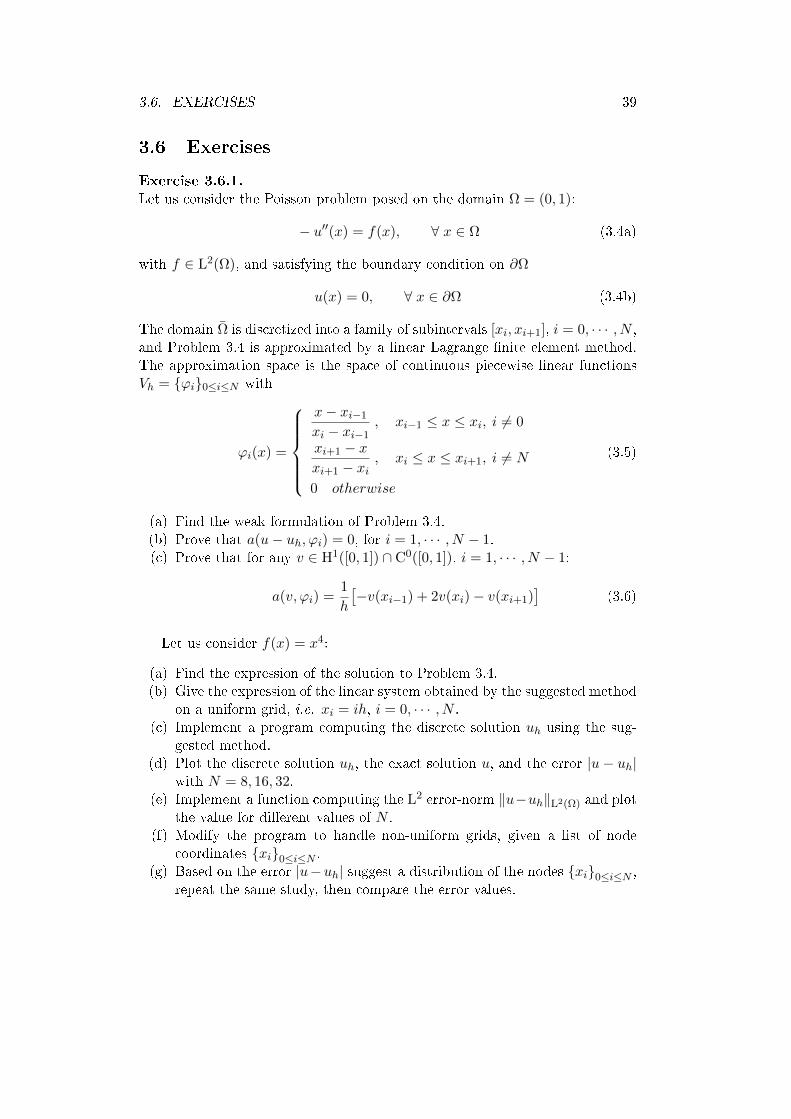
Exercise 3.6.1.

Let us consider the Poisson problem posed on the domain Ω = (0, 1):

− u′′(x) = f(x), ∀ x ∈ Ω (3.4a)


u(x) = 0, ∀ x ∈ ∂Ω (3.4b)

The domain Ω is discretized into a family of subintervals [xi, xi+1], i = 0, · · · , N ,and Problem 3.4 is approximated by a linear Lagrange nite element method.The approximation space is the space of continuous piecewise linear functionsVh = ϕi0≤i≤N with

ϕi(x) =

x− xi−1

xi − xi−1, xi−1 ≤ x ≤ xi, i 6= 0

xi+1 − xxi+1 − xi

, xi ≤ x ≤ xi+1, i 6= N

0 otherwise

(3.5)

(a) Find the weak formulation of Problem 3.4.(b) Prove that a(u− uh, ϕi) = 0, for i = 1, · · · , N − 1.(c) Prove that for any v ∈ H1([0, 1]) ∩ C0([0, 1]), i = 1, · · · , N − 1:

a(v, ϕi) =1

h

[−v(xi−1) + 2v(xi)− v(xi+1)

](3.6)

Let us consider f(x) = x4:

(a) Find the expression of the solution to Problem 3.4.(b) Give the expression of the linear system obtained by the suggested method

on a uniform grid, i.e. xi = ih, i = 0, · · · , N .(c) Implement a program computing the discrete solution uh using the sug-

gested method.(d) Plot the discrete solution uh, the exact solution u, and the error |u− uh|

with N = 8, 16, 32.(e) Implement a function computing the L2 error-norm ‖u−uh‖L2(Ω) and plot

the value for dierent values of N .(f) Modify the program to handle non-uniform grids, given a list of node

coordinates xi0≤i≤N .(g) Based on the error |u−uh| suggest a distribution of the nodes xi0≤i≤N ,

repeat the same study, then compare the error values.

Chapter 4

Simplicial Lagrange Finite

Elements

4.1 Denitions

Vector spaces of polynomials are used as approximation spaces to constructFinite Elements.

Denition 4.1.1 (Space of polynomials with real coecients). LetK ⊂ Rd, k ∈N, Pk(K) is the vector space of polynomials with real coecients of degree k onK, and the canonical basis is given by the family

xα1

1 · · ·xαii · · ·x

αdd : |α| = k

,

with xi the i-th coordinate of x ∈ Rd.

The dimension of the space is given by

dim(Pk(Rd)) =1

d!

d∏i=1

(k + i)

so that in particular dim(Pk(R1)) = k + 1, which means that such polynomialswill be uniquely dened by its values at k + 1 nodes.

Example 4.1.2. Linear and quadratic polynomials in dierent dimensions ofspace are listed below.

P1(R1) = span 1, xP1(R2) = span 1, x, yP1(R3) = span 1, x, y, zP2(R1) = span

1, x, x2

P2(R2) = span

1, x, y, xy, x2, y2

P2(R3) = span

1, x, y, z, xy, yz, xz, x2, y2, z2

Simplicial Lagrange Finite Elements are considered, for which the approxi-

mation space P will be polynomials on K, a d-simplex. Simplices are a general-ization of triangles to d dimensions, which consists of intervals (d = 1), triangles(d = 2), or tetrahedra (d = 3).

41

42 CHAPTER 4. SIMPLICIAL LAGRANGE FINITE ELEMENTS

Denition 4.1.3 (Simplex). Let vi0≤i≤d be a family of d + 1 points of Rdthat do not belong to the same hyperplane, the associated d-simplex K is theconvex hull of these points. Points vi are called vertices of the simplex, andpairs εij = (vi, vj), i 6= j, consist of the eddges. The diameter of the simplex isthe maximum Euclidean distance between two vertices,

diam(K) = max0≤i,j≤d

‖vi − vj‖

The convex hull is the minimum convex subset of Rd enclosing the points.The condition that all points are not in the same hyperplane means that theconvex hull does not degenerate into a lower-dimensional entity; for instance intwo dimensions, a triangle degenerates to a segment when points are aligned, andin three dimensions, a tetrahedron degenerates if all points are in the same plane.Therefore a degenerate simplex has a zero d-dimensional Lebesgue measure.

Consider the matrix Md of R(d+1)×(d+1) consisting of column vectors withcoordinates of vertices vi of K, and completed by a unit row.

M1 =

[x0 x1

1 1

]M2 =

x0 x1 x2

y0 y1 y2

1 1 1

M3 =

x0 x1 x2 x3

y0 y1 y2 y3

z0 z1 z2 z3

1 1 1 1

The determinant of Md gives the signed d-dimensional measure (volume) of

the corresponding simplex K.

det(Md) = ±d!|K|

In particular, if all the points are contained in the same hyperplane then anyvertex is the linear combinations of others so that the determinant is zero. Giventhat the sign of the determinant depends on permutations of the matrix Md, inpractice the meaning of the sign is the orientation of the simplex which dependson how vertices are numbered.

4.2 Polynomial interpolation in one dimension

Let Pk([a, b]) be the space of polynomials p =∑k

i=0 αixi of degre lower or equal

to k on the interval [a, b], with cixi the monomial of order i, ci a real number.

A natural basis of Pk([a, b]) consists of the set of monomials

1, x, x2, · · · , xk.

Its elements are linearly independent but in the frame of Finite Elements we canchose another basis which is the Lagrange basis

Lki

0≤i≤k of degree k denedon a set of k + 1 points ξi0≤i≤k which are called Lagrange nodes.

4.3. CONSTRUCTION OF THE FINITE ELEMENT SPACE 43

Denition 4.2.1 (Lagrange polynomials [4] page 21, [6] page 76). The La-grange polynomial of degree k associated with node ξm reads

Lkm(x) =

k∏i=0i 6=m

(x− ξi)

k∏i=0i 6=m

(ξm − ξi)

andk∑i=0

Lki (x) = 1

Proposition 4.2.2 (Nodal basis).

Lki (ξj) = δij , 0 ≤ i, j ≤ k

The following result gives a pointwise control of the interpolation error.

Theorem 4.2.3 (Pointwise interpolation inequality [6] page 79). Let u ∈Ck+1([a, b]) and πk u ∈ Pk([a, b]) its Lagrange interpolate of order k, with La-

grange nodes ξi0≤i≤k, then ∀ x ∈ [a, b]:

|u(x)− πk u(x)| ≤

∣∣∣∣∣k∏i=0

(x− ξi)

∣∣∣∣∣(k + 1)!

maxs∈[a,b]

∣∣∣∂k+1u(s)∣∣∣

4.3 Construction of the Finite Element space

4.3.1 A nodal element

Let us take ξ1, · · · , ξN a family of points of K such that σi(p) = p(ξi),1 ≤ i ≤ N :

• ξi1≤i≤N is the set of geometric nodes,

• ϕi1≤i≤N is a nodal basis of P, i.e. ϕi(ξj) = δij .

We can verify, for any p ∈ P that:

p(ξj) =

N∑i=1

σi(p) ϕi(ξi)︸︷︷︸δij

, 1 ≤ i, j ≤ N

which reduces to:p(ξj) = σi(p)

Remark 4.3.1 (Support of shape functions). The polynomial basis being de-ned such that ϕj(ξi) = δij then any shape function ϕi has support on theunion of cells containing the node ξi.


4.3.2 Reference Finite Element

To make the connection between the abstract Denition 3.3.1 and a simpleconcrete example, the reference element for Lagrange P1 in one dimension isgiven by the following triple (K, P, Σ).

Denition 4.3.2 ((K, P, Σ) for Lagrange P1 1D). The Finite Element spaceLagrange P1 1D approximating

Vh =v ∈ C0(Ω) ∩H1(Ω) : v|K ∈ P1(K), ∀ K ∈ Th

is given by

• K is the unit interval [0, 1].

• P is the space of linear polynomials P1([0, 1]) with the basis (ϕ0, ϕ1) byDenition 4.2.1 of L1

i ,

ϕ0(x) = L10(x) = 1− x, ϕ1(x) = L1

1(x) = x

• Σ is the set of linear forms evaluating the function at Lagrange nodesξ0 = 0 and ξ1 = 1, σ0 : v 7→ v(ξ0), σ1 : v 7→ v(ξ1).

Consequently the local interpolation operator is

IK,V : V (K) → Vh(K)

v 7→ v(ξ0)ϕ0 + v(ξ1)ϕ1

Proposition 4.3.3. (K,P,Σ) by Denition 4.3.2 is a unisolvent H1-conformal

Finite Element.

Proof. During the lecture we proved that:

• Vh ⊂ H1(Ω), since piecewise linear and piecewise constant functions belongto L2(Ω).

• (ϕi) is a basis of P1(K) since shape functions are linearly independent asthey satisfy ϕi(ξj) = δij , and they generate the space Vh as any piecewiselinear function coincides with its interpolate.

• (σi) is a dual basis of P1(K) since σi(ϕj) = δij .

4.3.3 Lagrange Pk elements

The extension to Lagrange Pk is natural as it boils down to construct a basisof Pk using (Lki )0≤i≤k and choose the degrees of freedom at the correspondingLagrange nodes ξi0≤i≤k. Given that the unisolvence for Lagrange P1 is adirect consequence of the construction from a nodal basis, the same argumentapplies for higher polynomial order as long as degrees of freedom are locatedat Lagrange nodes. As illustration Table 4.3.3 depicts the shape functions fork = 1, 2, 3 in one dimension with equidistributed nodes (but other distributionsare possible and also other polynomials can be used to build nodal elements).

4.4. EXTENSION TO MULTIPLE DIMENSIONS 45

P1

1

1ϕ0 ϕ1

P2

1

1ϕ0 ϕ1 ϕ2

P3

1

1ϕ0 ϕ1 ϕ2 ϕ3

Table 4.1: Shape functions for Lagrange P1,P2,P3 on the interval K = [0, 1].

4.4 Extension to multiple dimensions

4.4.1 Barycentric coordinates

Lagrange polynomials (4.2.1) construct directly one-dimensional shape func-tions, while in higher dimensions they can be reformulated in terms of barycen-


tric coordinates. High-order Lagrange basis can also be expressed as polynomialsof barycentric coordinates.

Denition 4.4.1 (Barycentric coordinates). Let us consider K a d-simplexwith vertices vi0≤i≤d, any point x ∈ K satises

x =∑i

λi(x)vi

where barycentric coordinates are obtained by relation

λi : Rd → R

x 7→ λi(x) = 1− (x− vi) · ni(vf − vi) · ni

with ni the unit outward normal to the facet opposite to vi, and vf a vertexbelonging to this facet.

The geometric interpretation of barycentric coordinates is given by

λi =meas(Ki)

|K|

with meas(Ki) the signed measure of Ki(x) the d-simplex constructed withpoint x and the facet opposite to vi. In particular, points located within Ki

have non-negative λi, and the point satisfying equal weight λi = (d+1)−1 is theisobarycentre. In practice this property can be used to check if a point is insidea simplex: if the signed measure of one λi is negative or if

∑i |Ki(x)| > |K|

then the point is outside of the simplex.

Example 4.4.2 (Lagrange P1 1D). In one dimension of space, barycentriccoordinates on K = [x0, x1] are

λ0(x) = 1− x− x0

x1 − x0=

x1 − xx1 − x0

λ1(x) = 1− x− x1

x0 − x1=

x− x0

x1 − x0

which is exactly the same expression as linear shape functions ϕ0 and ϕ1.

Example 4.4.3 (Lagrange P1 2D). In two dimensions of space, barycentriccoordinates on the unit triangle K depicted Figure 4.4.3 are

λ0(x) = 1− (x, y) · (1, 1)

(1, 0) · (1, 1)= 1− x− y

λ1(x) = 1− (x− 1, y) · (−1, 0)

(−1, 0) · (−1, 0)= x

λ2(x) = 1− (x, y − 1) · (0,−1)

(0,−1) · (0,−1)= y

which is the linear Lagrange basis on K (since the normal is at the numeratorand the denominator, there was no need to normalize the vector).

4.4. EXTENSION TO MULTIPLE DIMENSIONS 47

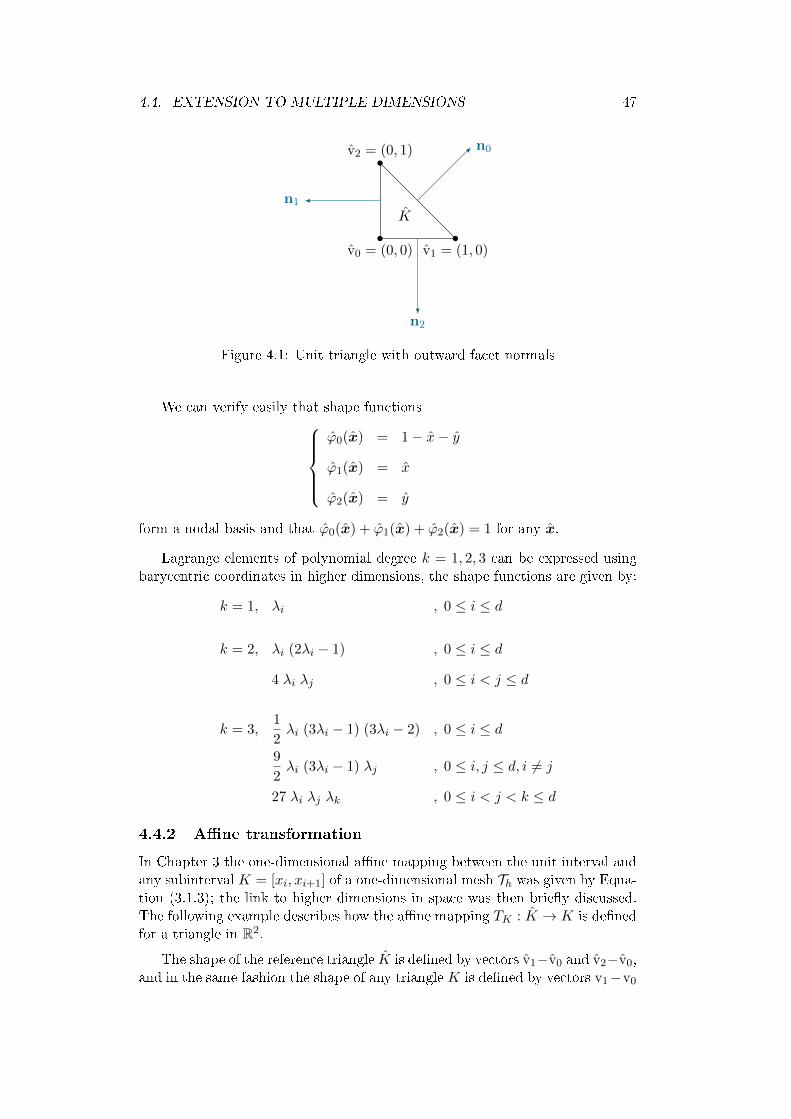
v0 = (0, 0) v1 = (1, 0)

v2 = (0, 1)

K

n0

n1

n2

Figure 4.1: Unit triangle with outward facet normals

We can verify easily that shape functionsϕ0(x) = 1− x− y

ϕ1(x) = x

ϕ2(x) = y

form a nodal basis and that ϕ0(x) + ϕ1(x) + ϕ2(x) = 1 for any x.

Lagrange elements of polynomial degree k = 1, 2, 3 can be expressed usingbarycentric coordinates in higher dimensions, the shape functions are given by:

k = 1, λi , 0 ≤ i ≤ d

k = 2, λi (2λi − 1) , 0 ≤ i ≤ d

4 λi λj , 0 ≤ i < j ≤ d

k = 3,1

2λi (3λi − 1) (3λi − 2) , 0 ≤ i ≤ d

9

2λi (3λi − 1) λj , 0 ≤ i, j ≤ d, i 6= j

27 λi λj λk , 0 ≤ i < j < k ≤ d

4.4.2 Ane transformation

In Chapter 3 the one-dimensional ane mapping between the unit interval andany subinterval K = [xi, xi+1] of a one-dimensional mesh Th was given by Equa-tion (3.1.3); the link to higher dimensions in space was then briey discussed.The following example describes how the ane mapping TK : K → K is denedfor a triangle in R2.

The shape of the reference triangle K is dened by vectors v1−v0 and v2−v0,and in the same fashion the shape of any triangle K is dened by vectors v1−v0


v0 = (0, 0) v1 = (1, 0)

v2 = (0, 1)

Kv0

v1

v2

K

TK

and v2−v0. The ane mapping is a simple change of coordinates but the detailis given below for the sake of completness.

v1 = TK(v1) = v0 + (v1 − v0)v2 = TK(v2) = v0 + (v2 − v0)

and any point x of K can be expressed in terms of the relation

x = v0 + λ(v1 − v0) + µ(v2 − v0)

with given λ and µ. The reference triangle is dened by the canonical basis ofR2 as (v1 − v0, v1 − v0) = (ex, ey) so that the ane mapping

x = v0 + BKx

satises TK(ex) = (v1 − v0) and TK(ey) = (v2 − v0). The matrix BK is thenthe matrix of the corresponding change of basis composed of column vectorsvj − v0, thus

x = v0 +

[v1,x − v0,x v2,x − v0,x

v1,y − v0,y v2,y − v0,y

]x

Denition 4.4.4 (Ane mapping from reference simplex in Rd). The general-ization of the ane mapping in Rd from the reference simplex K = vi0≤i≤dto K = vi0≤i≤d is given by x = v0 + JTK x, with

JTK =

[∂T iK∂xj

]ij

given by colum vectors (vj − v0).

While the change of coordinates for the mass matrix does not pose any dif-culty, the case of the stiness matrix requires some precisions. The derivationof the composition of two functions reads

∇ϕ = ∇(ϕ T−1K ) = (∇ϕ T−1

K ) · JT−1K

which can be also written formally component by component

∂ϕ

∂xi=∑j

∂ϕ

∂xj

∂xj∂xi

=∑j

∂ϕ

∂xjJT−1

K

4.5. LOCAL EQUATION FOR LAGRANGE P1 IN ONE DIMENSION 49

and can be interpreted as the decomposition of variation dx along each axisin terms of dx. Moreover the Jacobian matrix of the inverse mapping is theinverse of the Jacobian matrix

JT−1K

= (JTK T−1K )−1

so that∇ϕ = [(JTK T

−1K )−1]

T(∇ϕ T−1

K )

and since the Jacobian matrix is constant on each cell K, it can be simplied as

∇ϕ = [J−1TK

]T

(∇ϕ T−1K )

4.5 Local equation for Lagrange P1 in one dimension

The approximation of Problem (1.5) by Lagrange P1 elements on domain Ω =(0, 1) reads: ∣∣∣∣∣∣∣

Find u ∈ Vh, given f ∈ L2(Ω), such that:∫Ω∇u ·∇v dx =

∫Ωfv dx , ∀ v ∈ Vh

(4.1a)

with the approximation space Vh chosen as:

Vh =v ∈ C0(Ω) ∩H1

0(Ω) : v|K ∈ P1(K), ∀ K ∈ Th

(4.1b)

The interval Ω = [0, 1] is discretized by partitioning into disjoints subin-tervals [xn, xn+1], 1 ≤ n ≤ NK of length h = 1/NK . Steps to obtain a weakformulation and deriving a discrete problem were detailed in Section 3.1.

Expressing the local equation for any subinterval K = [xn, xn+1] consists ofassembling a matrix corresponding to contributions

Aij =

∫K∂xϕj(x) ∂xϕi(x) dx

for shape functions ϕj and ϕi which have support on K. Given that the di-mension of the Lagrange P1 element in one dimension is two, with two shapefunctions ϕn and ϕn+1, the local matrix is of dimension 2 × 2. The deriva-tive of ϕn and ϕn+1 is constant on K and of opposite signs: ϕn(x) = −1 andϕn+1(x) = +1.

AK =1

h

[+1 −1−1 +1

]with row and column indices of the local matrix mapping to row and columnindices (n, n+ 1) of the global matrix. Therefore assembling the local equationinto the global matrix consists of adding entries of AK to the submatrix with rowand column indices (n, n+1). Since each node xn has two adjacent subintervals[xn−1, xn] and [xn, xn+1], inner nodes (which are not on the boundary) will see


two contributions +1 on the diagonal, one contribution −1 for columns n − 1,and one contribution −1 for columns n+ 1, scaled by factor 1/h.

Ai =1

h

[0 · · · 0 −1 +2︸︷︷︸

aii

−1 0 · · · 0]

If the partition of the interval is not uniform then the assembly of the localequation should be modied,

AK =1

|K|

[+1 −1−1 +1

]with |K| = |xn+1 − xn|.

4.6. EXERCISES 51

4.6 Exercises

Exercise 4.6.1.

Let us consider the Helmoltz problem posed on the domain Ω = (0, 1), given κa real coecient:

− u′′(x) + κu(x) = f(x), ∀ x ∈ Ω (4.2a)

with f ∈ L2(Ω),u(x) = 0, ∀ x ∈ ∂Ω (4.2b)

Let us consider the analytic solution for κ = 1 and f(x) = sin(πx) given by

u(x) = sin(πx)/(1 + π2).

(a) Derive a weak formulation of Problem (4.2).(b) Show that the problem solved by a Galerkin method using the discrete

space Vh = span ϕi, 1 ≤ i ≤ N , can be written under the form of alinear system

(A + κM)u = b

(c) Express the linear system when the problem is approximated with Vh =X1h the space of linear Lagrange nite element on a uniform grid.

(d) Implement a program to solve the problem with Vh = X1h and compare

the discrete solution with the suggested analytic solution.(e) Express the linear system when the problem is approximated with Vh =

X2h the space of quadratic Lagrange nite element on a uniform grid.

(f) Modify the linear system for a general non-uniform grid, and for testinguse vertices:

V = 0.0, 0.1, 0.25, 0.3, 0.4, 0.45, 0.5, 0.55, 0., 6, 0.7, 0.8, 0.9, 1.0

(g) Write a function computing integrals by the quadrature formula:∫ 1

0g(x) dx ≈ 1

2

[g(c1) + g(c2)

], c1 =

1

2+

√3

6, c2 =

1

2−√

3

6

to approximate contributions for each element to the load vector b.(h) Implement a program to solve the problem with Vh = X2

h and comparethe discrete solution with the suggested analytic solution.

(i) Modify the program to implement the boundary condition u(0) = 1,u′(x) = 2. Which changes are required?

Appendix A

Denitions

A.1 Mapping

Denition A.1.1 (Mapping). Let E and F be two sets, a mapping

f : E → Fx 7→ f(x)

is a relation which, to any element x ∈ E, associates an element y = f(x) ∈ F .

Denition A.1.2 (Linear mapping). Let E and F be two K-vector spaces, themapping f : E → F is linear if:

1. ∀ x, y ∈ E, f(x+ y) = f(x) + f(y)

2. ∀ λ ∈ K, y ∈ E, f(λx) = λf(x)

A.2 Spaces

Denition A.2.1 (Vector space (on the left)). Let (K,+,×) be a eld i.e.

dened such that (K,+) is an Abelian additive group and (K \ 0K,×) is anAbelian multiplicative group, K = R or K = C.

(K,+) (K \ 0K,×)

+ commutative and associative × commutative and associative0K neutral for `+ 11K neutral for `×

+ admits an opposite × admits an inverse× is distributive with respect to +

(E,+, · ) is a vector space on (K,×) if:

1. (E,+) is an additive Abelian group (same properties as (K,+)).

2. The operation · : K× E → E satises:

distributive w.r.t +E on the left λ · (u+ v) = λ ·u+ λ · vdistributive w.r.t +K on the right (λ+ µ) ·u = λ ·u+ µ ·u

associative w.r.t × (λ× µ) ·u = λ · (µ ·u)11K neutral element on the left 11K ·u = u

53

54 APPENDIX A. DEFINITIONS

In short the vector space structure allows writing any u ∈ E as linear com-binations of elements vi of E called vectors with elements λi of K calledscalars as coecients,

u =∑i

λivi

and both the multiplications for vectors and scalars are distributive with respectto the additions. In this document we only consider real vector spaces, K = R.

Denition A.2.2 (Norm). Let E be a K-vector space, the application

‖ · ‖ : E → R+

is a norm if the following properties are satised:

1. Separation: ∀ x ∈ E, ( ‖x‖E = 0 )⇒ ( x = 0E )

2. Homogeneity: ∀ λ ∈ K, ∀ x ∈ E, ‖λx‖E = |λ| ‖x‖E

3. Subadditivity: ∀ x, y ∈ E, ‖x+ y‖E ≤ ‖x‖E + ‖y‖E

Note A.2.3. The third property is usually called triangle inequality.

Denition A.2.4 (Equivalent norms). Let E be a K-vector space, norm ‖ · ‖EEis said equivalent to ‖ · ‖E if there exist C1, C2 > 0 such that:

C1‖u‖E ≤ ‖u‖EE ≤ C2 ‖u‖E , ∀ u ∈ E

Denition A.2.5 (Seminorm). Let E be a K-vector space, the application

‖ · ‖ : E → R+

is a seminorm if it satises properties (A.2.2).2 and (A.2.2).3.

Denition A.2.6 (Scalar product). Let E be a R-vector space, the bilinearmapping

( · , · ) : E × E → R

is a scalar (or inner) product of E if it satises the following three properties:

1. Symmetry: ∀ x, y ∈ E, ( x , y ) = ( y , x )

2. Positivity: ∀ x ∈ E, ( x , x ) ≥ 0

3. Deniteness: ( ( x , x ) = 0 )⇔ ( x = 0 )

Appendix B

Duality

B.1 In nite dimension

Denition B.1.1 (Dual space). Let E be a nite dimensional real vector space,its dual E? is the space of linear forms on E, denoted by L(E;R).

Denition B.1.2 (Dual basis). Let E be a nite dimensional real vector space,dim(E) = N and B = (e1, · · · , eN ) a basis of E. Let us denote, for any i, j ∈[[1, N ]], by:

e?i : E → Rej 7→ δij

the i-th coordinate. The dual family of B, B? = (e?1, · · · , e?N ) is a basis of E?.

Thus we can write any element u ∈ E as:

u =N∑i=1

e?i (u)ei

Proving that B? is a basis of E? requires that ei generates E? and that itselements are linearly independent. The corollary of the rst condition is thatdim(B?) = N .

55

Appendix C

Function spaces

C.1 Banach and Hilbert spaces

Denition C.1.1 (Cauchy criterion). Let (E, ‖ · ‖E) be a normed vector spaceand (vn)n∈N be a sequence of element of E which satises:

∀ ε > 0, ∃N such that ∀ p, q ≥ N , ‖vp − vq‖E ≤ ε

then (vn)n∈N is a Cauchy sequence in E.

Denition C.1.2 (Banach space). A Banach space (E, ‖ · ‖E) is a normedvector space with is complete with respect to the norm ‖ · ‖E , i.e. Cauchysequences converge in E.

Denition C.1.3 (Hilbert space). Let E be a K-vector space and ( · , · ) bea sesquilinear form on the left (or bilinear form if K = R),

( x1 + x2 , y ) = ( x1 , y ) + ( x2 , y )

( x , y1 + y2 ) = ( x , y1 ) + ( x , y2 )

( λx , y ) = λ( x , y )

( x , λy ) = λ( x , y )

which is also positive denite on E,

∀ x 6= 0E , ( · , · ) > 0

then (E, ( · , · )) is a pre-Hilbertian space. Moreover, if E is complete withrespect to the norm dened by ( · , · ), it is a Hilbert space.

Denition C.1.4 (Hilbertian norm).

1

2

(‖x‖2E + ‖y‖2E

)= ‖x+ y

2‖2E + ‖x− y

2‖2E

57

58 APPENDIX C. FUNCTION SPACES

Remark C.1.5. This is basically the parallelogram identity stating that thesum of the square of the length diagonals is equal to the sum of the square of thelength of all the sides. This equality is useful to check that a norm is generatedfrom a scalar product. For Banach spaces like Lp, this becomes the Clarksoninequality.

Theorem C.1.6 (Projection on a convex subset). Let H be a Hilbert space and

K ⊂ H be a convex closed non-empty subset, ∀ x ∈ H there exists a unique

x0 ∈ K such that

‖x− x0‖H = infy∈K‖x− y‖H

with x0 the projection of x onto K and we denote it by x0 = PK x

C.2 Spaces of continuous functions

Ck(Ω) =u ∈ C0(Ω) : u′ ∈ Ck−1(Ω)

C∞c (Ω) = u ∈ C∞(Ω) with compact support in Ω

C.3 Lebesgue spaces

Lp(Ω) =

u :

∫Ω|u(x)|p dx <∞

Remark C.3.1. Lebesgue spaces Lp, 1 ≥ p ≥ ∞ are Banach spaces for thenorm

‖ · ‖Lp(Ω) =

(∫Ω|u(x)|p

)1/p

and L2 is a Hilbert space endowed with the scalar product

( u , v ) L2(Ω) =

∫Ωu v dx (C.1)

C.4 HilbertSobolev spaces

Hs(Ω) =u ∈ L2(Ω) : Dαu ∈ L2(Ω) , 1 ≤ α ≤ s

C.5 Sobolev spaces

Wm,p(Ω) = u ∈ Lp(Ω) : Dαu ∈ Lp(Ω) , 1 ≤ α ≤ m

Remark C.5.1. Hs spaces are Ws,2 spaces.

Appendix D

Inequalities

D.1 Useful inequalities in normed vector spaces

Lemma D.1.1 (CauchySchwarz). Let E be a K-vector space, any positive

sesquilinear form ( · , · ) on E satises the inequality:

|( u , v )E | ≤ ‖u‖E‖v‖E

Remark D.1.2. In particular any scalar product satises the CauchySchwarzinequality. For example:

( u , v ) L2(Ω) =

∫Ωu v dx ≤ ‖u‖L2(Ω)‖v‖L2(Ω)

Lemma D.1.3 (Young). Let a, b > 0 be two real numbers:

ab ≤ 1

p

(aγ

)p+

1

q

(bγ)q

with1

q+

1

p= 1 and γ > 0.

Remark D.1.4. In particular, the following inequality is commonly used forenergy estimates:

ab ≤ 1

2

(aγ

)2+

1

2(bγ)2

Lemma D.1.5 (Generalized Hölder). Let u ∈ Lp(Ω), v ∈ Lq(Ω), with 1 ≤ p <∞, then:

‖u v‖Lr(Ω) ≤ ‖u‖Lq(Ω)‖v‖Lq(Ω)

with1

r=

1

p+

1

q

Lemma D.1.6 (Minkowski).

‖u+ v‖Lp(Ω) ≤ ‖u‖Lp(Ω) + ‖v‖Lp(Ω)

59

60 APPENDIX D. INEQUALITIES

Remark D.1.7. The previous result is basically the triangle inequality for theLp norm.

Lemma D.1.8 (Poincaré). Let Ω be an open bounded subset, for any 1 ≤ p <∞there exists a constant real number cP > 0 such that ∀ u ∈W1,p

0 (Ω):

cP ‖u‖Lp(Ω) ≤ ‖∇u‖Lp(Ω)

Remark D.1.9. As a Corollary usefull for the Poisson problem that we address,we get that ‖∇u‖L2(Ω) denes an equivalent norm to ‖u‖1 on H1

0(Ω).

Lemma D.1.10 (Clarkson). Let 1 < p < ∞, and u, v be two functions of

Lp(Ω), then:

1. for p ≥ 2

‖u+ v

2‖2Lp(Ω) + ‖u− v

2‖2Lp(Ω) ≤

1

2

(‖u‖2Lp(Ω) + ‖v‖2Lp(Ω)

)2. for p < 2

‖u+ v

2‖2

Lp′ (Ω)+ ‖u− v

2‖2

Lp′ (Ω)≤(

1

2‖u‖2Lp(Ω) +

1

2‖v‖2Lp(Ω)

)1/(p−1)

Remark D.1.11. These inequalities are basically parallelogram inequalitiesgeneralized to Lp spaces.

Appendix E

Exercise solutions and hints

61

62 APPENDIX E. EXERCISE SOLUTIONS AND HINTS

E.1 Chapter 1

Solution E.1.1 (Exercise 1.6.1 page 14).

(a) False. Justify by verifying that linear combination of functions of S donot satisfy v(1

2) = 1.(b) True. Verify that the functional is linear, L(λu+ µv) = λL(u) + µL(v),(c) False. Show that ( · , · )V is not bilinear.(d) False. Verify that |u|H1(Ω) = 0 for u = c so it is not positive denite, only

positive: |·|H1(Ω) is a semi-norm for H1(Ω) but a norm for H10(Ω) since the

only constant satisfying the trace is u = 0.(e) Verify that the function and derivatives are square integrable:

‖v‖2L2((0,1)) =

∫ 1

0x3 dx =

2

3

|v|2H1((0,1)) =

∫ 1

0

9

16x−1/2 dx =

9

8

|v|2H2((0,1)) =

∫ 1

0

−9

32x−3/2 dx not bounded

(f) False. Express both semi-norm and compare that they are dierent sincethe derivation of the exponential gives a factor −10.


(a) To get the strong problem of (1.7) integate the second by part to get allthe derivatives on the solution. Since there is no linear form associatedwith Neumann boundary conditions and the solution space is H1

0(Ω) theboundary condition of the problem is an homogeneous Dirichlet conditionon ∂Ω.

κu′(x)− u′′(x) + u(x) = f(x), x ∈ Ω, u(0) = u(1) = 0

(b) Verify that the Problem (1.7) statises the hypothesis of the LaxMilgramtheorem.


(a) To derive a weak formulation, test the equation against v ∈ C∞c (Ω) andintegrate by part to report derivatives on v.

〈∆2u , v 〉 = ( ∆u , ∆v )

Given that C∞c (Ω) is dense in H2(Ω) it is then possible to nd∣∣∣∣∣∣∣Find u ∈ H2

0(Ω) such that:∫Ω

∆u∆v dx =

∫Ωfv dx , ∀ v ∈ H2

0(Ω)

E.1. CHAPTER 1 63

(b) The solution and test space are suggested to be H20(Ω) given that the

bilinear form is the L2 inner product of ∆u when v = u, and the boundaryconditions cancel the function and rst derivative.

(c) Given that the bilinear form is the inner product of H20(Ω) the Riesz the-

orem applies directly.


E.2 Chapter 2


(a) The minimization principle is J(u) ≤ J(u+ v), ∀ v ∈ V ,

J(u+ v) =1

2a(u+ v, u+ v)− L(u+ v)

J(u+ v) =1

2a(u, u)− L(u) +

1

2

(a(u, v) + a(v, u)

)− L(v) +

1

2a(v, v)

J(u+ v) = J(u) + a(u, v)− L(v)︸︷︷︸ 0 +1

2a(v, v)

and the last term is positive for v 6= 0 so

J(u+ v) > J(u)

for v 6= 0.(b) This is proved in Chapter 2 for the well-posedness of the Ritz problem,

the Euler condition is satised for vecvT

(Au − b) = 0, and conversely ifAu = b then u is a minimizer of the quadratic form in RN .

E.3. CHAPTER 3 65

E.3 Chapter 3

Solution E.3.1 (Exercise 3.6.1 page 39).The solution to the exercise is given by Section 3.1 and Section 4.5.


E.4 Chapter 4

Bibliography

[1] F. Boyer and P. Fabrie. Mathematical Tools for the Study of the Incompress-

ible NavierStokes Equations and Related Models, volume 183 of SpringerSeries: Applied Mathematical Sciences. Springer, 2013.

[2] S. Brenner and R. Scott. The Mathematical Theory of Finite Element Meth-

ods, volume 15 of Springer Series: Texts in Applied Mathematics. Springer,2008.

[3] H. Brezis. Functional Analysis, Sobolev Spaces and Partial Dierential Equa-tions. Springer, 2011.

[4] A. Ern and J.-L. Guermond. Theory and Practice of Finite Elements, volume159 of Springer Series: Applied Mathematical Sciences. Springer, 2004.

[5] R. Herbin. Analyse Numérique des EDPs. Notes de cours de Master 2,Université de Provence, 2006.

[6] P. Hansbo K. Eriksson, D. Estep and C. Johnson. Computational Dierential

Equations. Press Syndicate of the University of Cambridge, 1996.

[7] J.-C. Latché. Méthodes d'Éléments Finis pour quelques problèmes elliptiqueslinéaires issus de la mécanique des uides. Notes de cours de Master 2,Université de Provence, 2002.

[8] A. T. Patera. Finite Element Methods for Elliptic Problems. Lecture Notes,MIT OpenCourseWare, 2003.

67

numerical solution of partial di erential equations using ... · contents contents 2 1 weak...

Documents