numerical solution for hydrodynamical models of … · cron devices, and several relevant physical...

August 23, 2000 11:26 WSPC/103-M3AS 00055

Mathematical Models and Methods in Applied SciencesVol. 10, No. 7 (2000) 1099–1120c© World Scientific Publishing Company

NUMERICAL SOLUTION FOR HYDRODYNAMICAL

MODELS OF SEMICONDUCTORS

VITTORIO ROMANO∗

Dipartimento Interuniversitario di Matematica,Politecnico di Bari, via E.Orabona 4-70125 Bari, Italy

GIOVANNI RUSSO†

Dipartimento di Matematica, Universita dell’Aquila,Via Vetoio, loc. Coppito-67100 L’Aquila, Italy

Communicated by P. A. Markowich

Received 23 November 1998Revised 14 June 1999

Numerical solutions of recent hydrodynamical models of semiconductors are computedin one-space dimension. Such models describe charge transport in semiconductor de-vices. Two models are taken into consideration. The first one has been developed byBlotekjaer, Baccarani et al., and the second one by Anile et al. In both cases the systemof equations can be written as a convection-diffusion type system, with a right-handside describing relaxation effects and interaction with a self-consistent electric field. Thenumerical scheme is a splitting scheme based on the Nessyahu–Tadmor scheme for the

hyperbolic step, and a semi-implicit scheme for the relaxation step. The numerical resultsare compared to detailed Monte–Carlo simulation.

1. Introduction

Charge transport in semiconductors has recently become an interesting research

field in applied mathematics.

The model that has been used in engineering applications is the so-called

drift-diffusion model.1,2 Such model, however, is not accurate enough for submi-

cron devices, and several relevant physical effects, such as inertial effects, are not

captured by this model.

For devices with channel length of some tenths of micron, when direct quan-

tum effects are negligible, an accurate physical description is given by semiclassical

kinetic models. The carriers are described by a density function in phase space,

∗E-mail: [email protected]†E-mail: [email protected]

1099

August 23, 2000 11:26 WSPC/103-M3AS 00055

1100 V. Romano & G. Russo

satisfying a Boltzmann-like equation. The most effective technique for the numer-

ical solution of such equation is Monte–Carlo simulation. However, computational

times required for an accurate solution are too large for a widespread use of Monte–

Carlo simulation as a practical CAD tool of semiconductor devices. It is therefore

desirable to approximate the transport equation with simpler models which are ac-

curate enough to maintain relevant physical effects of charge transport in submicron

devices, and much faster to solve than kinetic models.

The drift-diffusion models can be derived from the kinetic equation by the

Chapman–Enskog expansion.3 These models are commonly used for device simu-

lations. They provide a reasonable approximation when the channel length is large

enough (say more than a few microns) with applied voltage of the order of one Volt.

The evolution of the carriers is described by a balance equation, where the current

is assumed a function of the density and density gradient.

With the reduction of the size of the devices, and the increase in electric field,

the drift-diffusion approximation is no longer satisfying, and more sophisticated

models are necessary, which are able to describe carrier evolution under the effect

of high electric field.

Blotekjaer,4 Baccarani and Wordeman5 proposed a model (BBW) which is the

analogue of the classical Navier–Stokes–Fourier model for dissipative fluids.

In BBW model, electrons are treated as an inviscid, thermal conducting,

monoatomic gas. Heat flux is given by an empirical Fourier law, with a thermal

conductivity that contains a fitting parameter. The latter is chosen to fit exper-

imental data or Monte–Carlo simulations. This expression for the heat flux has

been recently criticized by Stettler6 and Tang,7 who suggest to add an empirical

convective term in the heat flux.

Anile et al.8 (which we denote by AP) proposed a model based on extended

thermodynamics .9,10 They obtain in a consistent way an expression for the heat

flux which contains a convective term, and has no fitting parameter, because all

transport coefficients are obtained from the theory.

In this paper we perform a numerical integration of the equations of AP and

BBW models. As a test problem we consider the simulation of a n+–n–n+ diode

in 1-D. The time-dependent problem is solved. The stationary solution is obtained

as a limit of the time-dependent solution for large enough time. The numerical

solutions are then compared with detailed Monte–Carlo simulations obtained by

the DAMOCLES code developed by IBM.11,12

The mathematical structure of the system of equations is the same for both

models. The differential part of the system can be written as a sum of hyperbolic

and parabolic terms. The right-hand side contains a relaxation term, which de-

scribes the interaction with the lattice, and a drift term due to the electric field.

The latter is self-consistently computed via Poisson’s equation.

The numerical scheme used is based on a splitting scheme. In the first step the

hyperbolic part is solved, and in the second step diffusion, relaxation, and drift

terms are computed. The hyperbolic step is solved by a variant of second-order

August 23, 2000 11:26 WSPC/103-M3AS 00055

Numerical Solution for Hydrodynamical Models of Semiconductors 1101

shock-capturing TVD scheme, recently developed by Nessyahu and Tadmor.13 A

uniformly non oscillatory reconstruction from cell averages is used.

A similar problem was consider in Ref. 14 by using ENO schemes. The choice

of the NT scheme is motivated by the following considerations. First we observe

that, because of the convective term in the heat flux for AP model, the hyperbolic

part of the equations is different from that of Euler’s equations and there is no

simple analytical expression of the characteristic speeds. The second reason is that

more complex models can be derived by extended thermodynamics.15 They are

described by hyperbolic systems with relaxation, and also in this case there is

no simple expression for the characteristic speeds, therefore it is not practical to

use upwind-based methods. NT scheme does not require the computation of the

eigenvalues of the system, since the building block is Lax–Friedrichs scheme.

The plan of the paper is as follows: In Sec. 2 we briefly recall the kinetic formu-

lation, the drift-diffusion model, and the two hydrodynamical models (BBW and

AP). In Sec. 3 we describe the numerical method used in the computation and

Sec. 4 is devoted to the numerical results.

2. Mathematical Models for Semiconductors

In a doped semiconductor, the carriers (electrons and holes) move under the influ-

ence of the electric field, and interact with phonons and impurities of the crystal.

Energy transport in crystal is mainly carried by phonons.16 A detailed physical

description of transport phenomena requires a three-component model — electrons,

phonons and holes, each of which satisfies a quantum transport equation coupled

with Maxwell’s equations for the electromagnetic field.

Carrier speed is at least three orders of magnitude smaller than light speed,

and therefore it is justified to neglect effect of the magnetic field induced by the

currents. A quasistatic approximation is assumed, where the self-consistent electric

field E is coupled to the system through the Poisson equation.

Furthermore, we shall neglect generation-recombination effects, whose charac-

teristic time is of the order of nanoseconds. The relaxation of our system, in fact,

takes place in times of the order of few picoseconds.

From now on we consider only one family of carriers, namely electrons. We shall

assume that phonons are in thermodynamical equilibrium and neglect the effect of

the heating of the crystal. Therefore the phonons are described by an equilibrium

distribution at temperature T0.

In a semiclassical kinetic description, the electron dynamics is described by a

transport equation for a one-particle distribution function f(x, t,k), which repre-

sents the probability density to find a particle at time t at position x and with

momentum k,

∂f

∂t+ vi(k)

∂f

∂xi− eEi ∂f

∂ki= C[f ] . (2.1)

August 23, 2000 11:26 WSPC/103-M3AS 00055


Here e represents the (positive) electron charge, E the electric field, k the electron

impulse, belonging to the first Brillouin zone.2,a

C[f ] is the collision term that describes the scattering with acoustical and optical

phonons. Electron velocity v(k) depends on the energy of the conduction band via

the dispersion relation,

v(k) = ∇kE .

In general, the band structure may be very complicated and depends on the type

and doping of the semiconductor. We shall consider a single band with parabolic

approximation. The energy is therefore given by

E =k2

m∗,

where m∗ is electron effective mass. In this approximation, electron velocity is given

by

vi =ki

m∗.

Consistently, the first Brillouin zone is extended to R3.

Equation (2.1) is a nonlinear integrodifferential equation in seven variables and

its use as a CAD tool is not practical on account of the numerical difficulties

which require too expensive computing time. This has prompted the formulation

of macroscopic models.

By introducing electron number density n and flux F by

n =

∫dkf and F =

∫dk

kf

m∗,

and integrating Eq. (2.1) with respect to k one obtains the balance equation for

the density

∂n

∂t+∂F i

∂xi= R−G , (2.2)

where R − G is the electron-hole generation-recombination term (which we shall

neglect).

Under the assumption that the electron temperature is equal to the (constant)

lattice temperature T0, and by introducing the mobility

µn =(4π)2e

3m∗kBT0n

∫dk feqk

4τ(E(k)) ,

one obtains

F = µnn∇φ−Dn∇n , (2.3)

where the diffusion coefficient is given by Dn = µnkBT0/e.

aEinstein summation over repeated indices is assumed. Physical units are such that ~ = 1.

August 23, 2000 11:26 WSPC/103-M3AS 00055


Equation (2.3), coupled with the analogue equation for holes and with the

Poisson equation, constitute the well-known drift-diffusion model.1,2

For submicron devices, with electric potential of the order of 1 V, the assumption

of constant electron temperature is no longer valid, since the electric field is strong

enough to prevent thermodynamical equilibrium. It is therefore necessary to have a

more detailed description of transport phenomena. Modified versions of the classical

drift-diffusion model have been proposed, which include some effects related to

temperature gradients.17,18 However hydrodynamical models seem more suitable

to describe nonequilibrium effects. In BBW model, electrons are treated as an

inviscid, thermal conducting fluid. The system is described by continuity equation,

momentum balance equation and energy balance equation,

∂

∂tn+

∂

∂xi(nvi) = 0 , (2.4)

∂

∂t(nvi) +

∂

∂xj

(nvivj +

p

m∗δij

)= −nvi

τp− neEi , (2.5)

∂

∂t

(nv2

2+

3

2

p

m∗

)+

∂

∂xi

[(nv2

2+

5p

2m∗

)vi +

qi

m∗

]= −W −W0

m∗τW− neviE

i

m∗,

(2.6)

coupled to the Poisson equation

ε∆φ = −e(ND −NA − n) .

Here NA is the acceptor density, ND the donor density, ε the dielectric constant,

W0 = 32nkBT0. W is the energy density given by

W =1

2nm∗v2 +

3

2nkBT ,

where T is the electron temperature, which is related to the pressure p by ideal gas

law

p = nkBT .

The heat flux satisfies Fourier’s law

qi = −kn ∂T∂xi

,

where

k =

(5

2+ c

)k2

B

Tτp

m∗.

c is a free parameter, whose value is chosen in order to fit experimental data or

Monte–Carlo simulations.

August 23, 2000 11:26 WSPC/103-M3AS 00055


Relaxation times are given by the following phenomenological expressions

τp =m∗µnT0

eT,

τW = µnT0

(m∗

2eT+

3kBT

2ev2S(T + T0)

),

where µn is low field mobility and vS is the saturation velocity.

BBW equations have been solved numerically in both the stationary19,20 and

nonstationary cases.14

This model, however, does not have the correct limit near thermodynamical

equilibrium,21 since it does not satisfy Onsager’s reciprocity conditions.22 Moreover,

the constitutive assumption on the heat flux has no theoretical justification.

A recent formulation of constitutive equations, in better agreement with the lin-

ear theory of irreversible process, has been obtained for the heat flux by Anile et al.8

The formulation is based on the theory of extended thermodynamics9,10 (the same

derivation can be obtained by the moment method approach of Levermore23).

The model is constituted, as for the BBW one, by the balance equations of

electron density, momemtum and energy

∂

∂tn+

∂

∂xi(nvi) = 0 , (2.7)

∂

∂t(nvi) +

∂

∂xjFij = Qi − neEi , (2.8)

∂

∂t

(nv2

2+

3

2

p

m∗

)+

∂

∂xiSi = −W −W0

m∗τW− neviE

i

m∗, (2.9)

where, according to the kinetic theory of gases,

Fij =

∫dkfkikj(m∗)2

is the flux momentum density and

Si =1

2

∫dkfkik

2

(m∗)3

is flux energy density.

By employing the methods of extended thermodynamics, followed by the so-

called Maxwellian iteration8,21,24 (a procedure similar to the Chapman–Enskog

expansion of the Boltzmann equation), the following relations have been obtained8

Fij = nvivj +p

m∗δij ,

Si =1

2nv2vi +

1

m∗

(5

2pvi + qi

),

August 23, 2000 11:26 WSPC/103-M3AS 00055


with the following constitutive equation for the heat flux qi

qi = −5nk2BTτq

2m∗∂T

∂xi+

5

2nkBTvi

(1

τp− 1

τq

)τq , (2.10)

τq being the energy flux relaxation time.

At variance with BBW model, Eq. (2.10) does not contain free parameters.

Moreover, due to the presence of the convective term in the constitutive equation

for the heat flux, Onsager relations for small deviations from thermodynamical

equilibrium are satisfied.21

About production terms, we shall use the same approximation used in BBW,

but with relaxation times given by Monte–Carlo simulation.

3. Numerical Method

Let us write the 1-D version of the equations of the two models:

∂

∂tn+

∂

∂x(nv) = 0 , (3.11)

∂

∂t(nv) +

∂

∂x

(nv2 +

p

m∗

)= −nv

τp− neE , (3.12)

∂

∂t

(nv2 + 3

p

m∗

)+

∂

∂x

(nv3 +

5pv

m∗+

2q

m∗

)= −2

W −W0

m∗τW− 2nevE

m∗. (3.13)

Heat flux q is given by

q = −5nk2BTτq

2m∗∂T

∂x+

5

2nkBTv

(τq

τp− 1

)(3.14)

for AP model and by

q = −(

5

2+ c

)nk2

B

Tτp

m∗∂T

∂x

for BBW model. The equations must be supplemented with Poisson’s equation.

For future reference it is better to write the previous equations in a more

compact form. Let us define the following vector fields:

u = (n, nv, 2W ) ,

fBBW =

(nv, nv2 +

p

m∗, nv3 +

5pv

m∗

),

fAP =

(nv, nv2 + 3

p

m∗, nv3 + 5

pv

m∗τq

τp

),

gBBW =

(0,−nv

τp− nE

m∗,−2

W −W0

m∗τw− 2nvE

m∗+

2

m∗∂

∂x

(kn∂T

∂x

)),

gAP =

(0,−nv

τp− nE

m∗,−2

W −W0

m∗τw− 2nvE

m∗+

1

m∗∂

∂x

(5nk2

BTτq

m∗∂T

∂x

)).

August 23, 2000 11:26 WSPC/103-M3AS 00055


The systems are then written as

∂u

∂t+∂fBBW

∂x= gBBW (3.15)

for BBW model and

∂u

∂t+∂fAP

∂x= gAP (3.16)

for AP model.

The left-hand side of Eqs. (3.15) and (3.16) represents a quasilinear hyperbolic

operator, while the right-hand side contains relaxation, diffusion and drift terms.

We make use of a splitting scheme, based on the following decomposition. Let us

consider a system of the form

∂u

∂t+∂f

∂x= g . (3.17)

Then, for each time step, a numerical approximation u of the solution is obtained

by solving the two consecutive steps:

∂u1

∂t+∂f

∂x= 0

u1(t) = u(t)

convection step (3.18)

∂u

∂t= g

u(t) = u1(t+ ∆t) .

relaxation step (3.19)

We shall call this scheme simple splitting (SP). Note that this scheme is only first

order in time, independently of the accuracy of the solution of the two steps.

A better scheme is obtained by a more sophisticated splitting strategy, as shown

in Sec. 3.3.

3.1. Convection step

During the convection step one integrates the quasilinear hyperbolic system (3.18).

It is well known that the solutions of such systems suffer loss of regularity and may

develop discontinuities. There is a wide literature on shock capturing schemes for

hyperbolic systems of conservation laws, which are second-order accurate in space in

the region of regularity, and give sharp shock profile. A recent account on numerical

methods for conservation laws was given in Ref. 25. Higher order methods have been

developed and used for solving problems in semiconductor device simulation, such as

ENO schemes (see Ref. 14). Such schemes, however, require an exact or approximate

Riemann solver, or at least the knowledge of the characteristic structure of the

Jacobian matrix. For systems similar to gas dynamics, an approximate Riemann

solver based on the Roe matrix is used. Such approach is suitable in the case of BBW

model, since the hyperbolic operator is the same as the one in gas dynamics, and

August 23, 2000 11:26 WSPC/103-M3AS 00055


x x

x xjj-1

j+1/2j-1/2

t

t

n+1

n

Fig. 1. NT scheme on a staggered grid.

therefore the analytical expression for the eigenvalues and eigenvectors is explicitly

known. In AP model, the presence of the term τq/τp does not allow us to write

down a simple analytical expression for the eigenvalues of the system (see Sec. 3.2).

Therefore it is desirable to use a shock-capturing scheme that does not require

the explicit knowledge of the characteristic structure of the system. The scheme

proposed by Nessyahu and Tadmor (NT)13 has these properties. Its building block

is Lax–Friedrichs scheme, corrected by a MUSCL type interpolation that guarantees

second-order in smooth regions and TVD property.26

For the sake of completeness, we report the derivation of NT scheme and UNO

reconstrution. For more details, see Refs. 13 and 27.

Let us consider a system of the form

∂v

∂t+∂f(v)

∂x= 0 , (3.20)

where v ∈ Rm and f : Rm → Rm. We introduce a uniform grid in x, x1, x2, . . . , xN ,

and in t, t1, t2, . . . .

By integrating Eq. (3.20) on a cell [xj , xj+1]× [tn, tn+1], one obtains

vj+1/2(tn + ∆t)

= vj+1/2(tn)− 1

∆x

[∫ tn+∆t

tn

f(v(xj+1, τ)) dτ −∫ tn+∆t

tn

f(v(xj , τ)) dτ

],

(3.21)

where

vj+1/2(tn) =1

∆x

∫ xj+1

xj

v(y, tn) dy

August 23, 2000 11:26 WSPC/103-M3AS 00055


represents the cell average of v(x, t) in [xj , xj+1] for t = tn. The integral of the flux

f(v(x, t)) is computed by the midpoint quadrature rule:∫ tn+∆t

tn

f(v(xj , τ)) dτ = ∆tf

(v(xj , tn +

∆t

2

)+O(∆t3) . (3.22)

The quantity v(xj , tn+∆t/2), is computed according to Lax–Wendroff approach,

by using Taylor’s formula:

v

(xj , t+

∆t

2

)= vj(t)−

1

2λf ′j +O(∆t2) , (3.23)

where f ′j/∆x is an approximation of the space derivative of the flux (yet to be

specified) and λ = ∆t/∆x. In order to obtain a second-order scheme we require

that

1

∆xf ′j =

∂

∂xf(v(x, t)) +O(∆x) .

By substituting (3.22) into (3.21), one has a relation that involves both cell averages

and point values of the solution.

By introducing a MUSCL interpolation, we approximate v(x, t) by a piecewise

linear polynomial

Lj(x, t) = vj(t) + (x− xj)1

∆xv′j , xj−1/2 ≤ x ≤ xj+1/2 (3.24)

and in order to ensure a second-order accuracy we require that

1

∆xv′j =

∂

∂xv(xj , t) +O(∆x) . (3.25)

Therefore, Eq. (3.21), together with (3.22)–(3.24), gives

vj+1/2(t+ ∆t) =1

2[vj(t) + vj+1(t)] +

1

8[v′j − v′j+1]

−λ[f

(vj+1(tn)− 1

2λf ′j+1

)− f

(vj(tn)− 1

2λf ′j

)]+O(∆t3) .

Since the initial state at t = tn is given by the piecewise linear function Lj(x, tn),

the fluxes remain regular functions if the solutions of the corresponding generalized

Riemann problems between adjacent cells do not interact.

This is obtained by imposing the following CFL condition

λ · ρ(A(v(x, t))) <1

2, (3.26)

where ρ(A(v(x, t))) is the spectral radius of the Jacobian matrix,

A =∂f

∂v.

August 23, 2000 11:26 WSPC/103-M3AS 00055


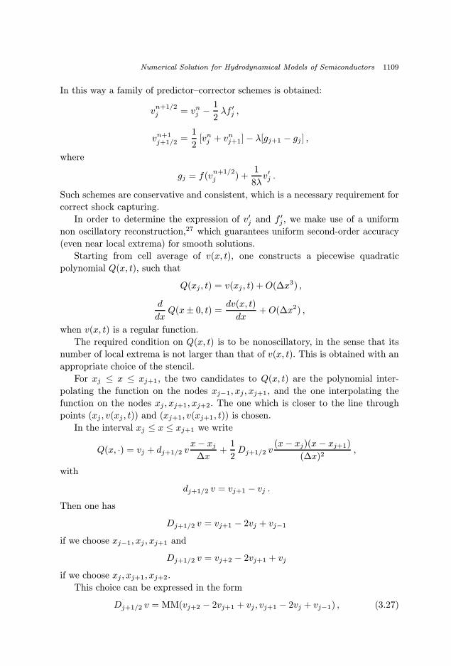
In this way a family of predictor–corrector schemes is obtained:

vn+1/2j = vnj −

1

2λf ′j ,

vn+1j+1/2 =

1

2[vnj + vnj+1]− λ[gj+1 − gj ] ,

where

gj = f(vn+1/2j ) +

1

8λv′j .

Such schemes are conservative and consistent, which is a necessary requirement for

correct shock capturing.

In order to determine the expression of v′j and f ′j , we make use of a uniform

non oscillatory reconstruction,27 which guarantees uniform second-order accuracy

(even near local extrema) for smooth solutions.

Starting from cell average of v(x, t), one constructs a piecewise quadratic

polynomial Q(x, t), such that

Q(xj , t) = v(xj , t) +O(∆x3) ,

d

dxQ(x± 0, t) =

dv(x, t)

dx+O(∆x2) ,

when v(x, t) is a regular function.

The required condition on Q(x, t) is to be nonoscillatory, in the sense that its

number of local extrema is not larger than that of v(x, t). This is obtained with an

appropriate choice of the stencil.

For xj ≤ x ≤ xj+1, the two candidates to Q(x, t) are the polynomial inter-

polating the function on the nodes xj−1, xj , xj+1, and the one interpolating the

function on the nodes xj , xj+1, xj+2. The one which is closer to the line through

points (xj , v(xj , t)) and (xj+1, v(xj+1, t)) is chosen.

In the interval xj ≤ x ≤ xj+1 we write

Q(x, ·) = vj + dj+1/2 vx− xj

∆x+

1

2Dj+1/2 v

(x− xj)(x− xj+1)

(∆x)2,

with

dj+1/2 v = vj+1 − vj .

Then one has

Dj+1/2 v = vj+1 − 2vj + vj−1

if we choose xj−1, xj , xj+1 and

Dj+1/2 v = vj+2 − 2vj+1 + vj

if we choose xj , xj+1, xj+2.

This choice can be expressed in the form

Dj+1/2 v = MM(vj+2 − 2vj+1 + vj , vj+1 − 2vj + vj−1) , (3.27)

August 23, 2000 11:26 WSPC/103-M3AS 00055


where MM(x, y) is the min mod function, defined by

MM(x, y) =

{sgn(x) ·min(|x|, |y|) if sgn(x) = sgn(y)

0 otherwise .

We can compute the slope of Lj(x, t) by

v′j∆x

= MM

(d

dxQ(xj − 0, t),

d

dxQ(xj + 0, t)

),

that is by

v′j = MM

(dj−1/2 v +

1

2MM(Dj−1, Dj), dj+1/2 v −

1

2MM(Dj , Dj+1)

), (3.28)

where

Dj = vj+1 − 2vj + vj−1 .

The computation of f ′j can be obtained by a similar reconstruction, from the values

of f(vnj ), or by the Jacobian matrix

f ′j =∂f

∂v(vj)v

′j .

Due to the staggered grid, we perform the convection step by two NT steps, so

that the field for the relaxation step is computed on a non-staggered grid.

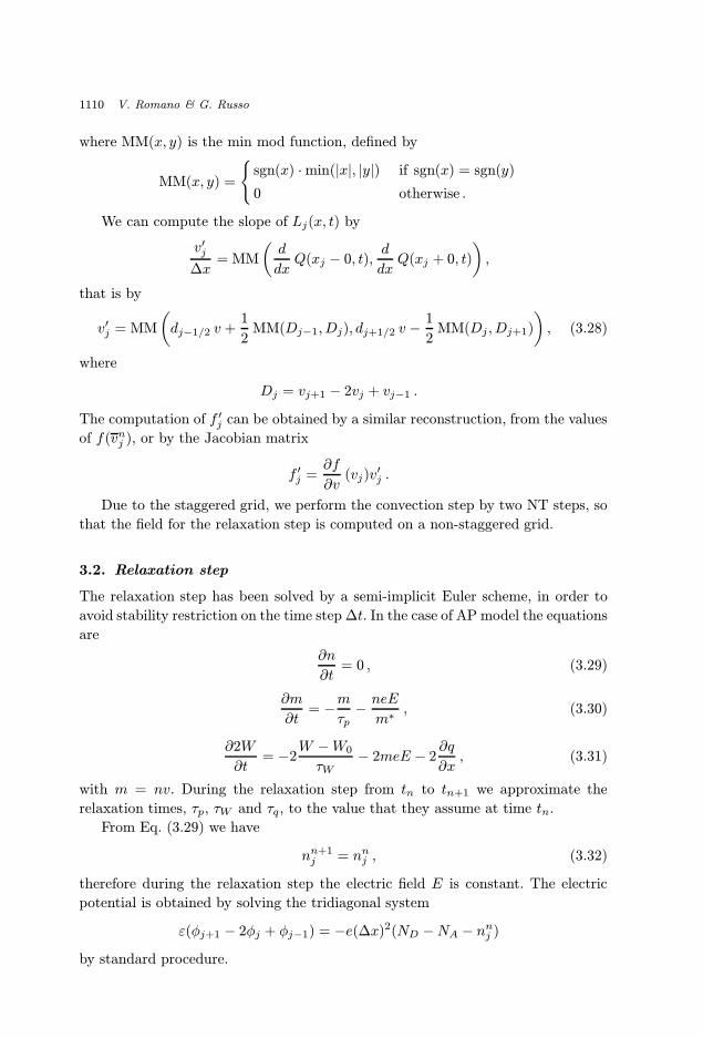
3.2. Relaxation step

The relaxation step has been solved by a semi-implicit Euler scheme, in order to

avoid stability restriction on the time step ∆t. In the case of AP model the equations

are

∂n

∂t= 0 , (3.29)

∂m

∂t= −m

τp− neE

m∗, (3.30)

∂2W

∂t= −2

W −W0

τW− 2meE − 2

∂q

∂x, (3.31)

with m = nv. During the relaxation step from tn to tn+1 we approximate the

relaxation times, τp, τW and τq, to the value that they assume at time tn.

From Eq. (3.29) we have

nn+1j = nnj , (3.32)

therefore during the relaxation step the electric field E is constant. The electric

potential is obtained by solving the tridiagonal system

ε(φj+1 − 2φj + φj−1) = −e(∆x)2(ND −NA − nnj )

by standard procedure.

August 23, 2000 11:26 WSPC/103-M3AS 00055


The electric field is computed from the potential by centered differences.

From Eq. (3.30) one has

mn+1j =

(mnj +

njeEnj τ

npj

m∗

)exp

(−∆t

τnpj

)−nnj eE

nj

m∗τnpj .

It is more convenient to integrate an equation for the temperature T , rather than

Eq. (3.31),

∂T

∂t=

1

3

m∗

kB

(2

τp− 1

τW

)v2 − T − T0

τW+

5kB

3nm∗∂

∂x

[nτqT

∂T

∂x

]. (3.33)

Let

A =5kB

3nm∗,

H =1

3

m∗

kB

(2

τp− 1

τW

)v2 +

T0

τW,

G = nτq .

Then Eq. (3.33) is discretized as

Tn+1j − Tnj

∆t= −

Tn+1j

τWj

+Aj

(∆x)2[(GT )nj+1/2(Tn+1

j+1 − Tn+1j )

− (GT )nj−1/2(Tn+1j − Tn+1

j−1 )] +Hj ,

where, for any quantity h defined on the grid, we denote

hj+1/2 ≡hj+1 + hj

2.

Once again we obtain a tridiagonal system for T n+1j which can be solved by

standard technique.

A similar procedure has been used in order to integrate the BBW equations.

Note that the relaxation step is second-order accurate in space, but only first

order accurate in time. However, it can be used to construct second-order schemes,

as described in Sec. 3.3.

3.3. Second-order splitting

Because of the splitting, scheme SP is not second-order accurate even for the

computation of steady state solutions.

Accuracy can be improved by using a better splitting strategy.

A second-order scheme, uniformly accurate in the relaxation times, has been

developed in Ref. 28 for a second-order upwind convection step. Different splitting

methods, that use the NT convection step, have been considered in Ref. 29.

A suitable generalization to the case where an electric field is present, is given

by the following steps: Given the fields at time tn, (Un, En), the fields at time tn+1

August 23, 2000 11:26 WSPC/103-M3AS 00055


are obtained as

U1 = Un −R(U1, En,∆t) ,

U2 =3

2Un − 1

2U1 ,

U3 = U2 −R(U3, En,∆t) ,

U4 = C∆tU3 ,

En+1 = P(U4) ,

Un+1 = U4 −R(Un+1, En+1,∆t/2) ,

where R represents the numerical operator corresponding to relaxation step, C∆trepresents the numerical convection operator corresponding to two steps of NT

scheme, P(U) gives the solution of Poisson’s equation.

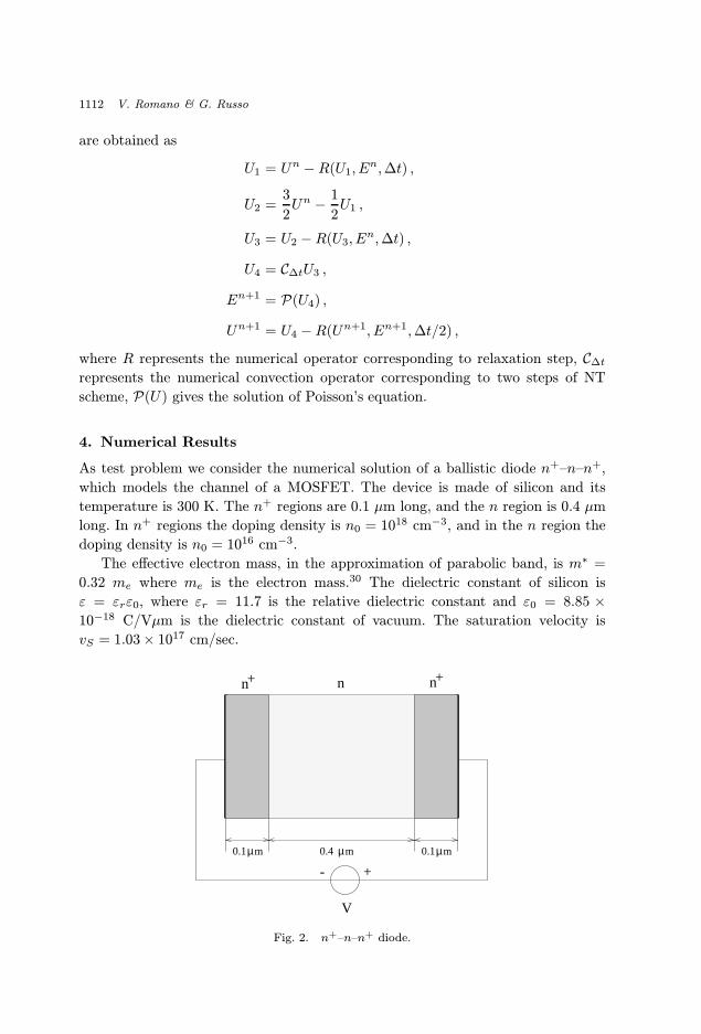
4. Numerical Results

As test problem we consider the numerical solution of a ballistic diode n+–n–n+,

which models the channel of a MOSFET. The device is made of silicon and its

temperature is 300 K. The n+ regions are 0.1 µm long, and the n region is 0.4 µm

long. In n+ regions the doping density is n0 = 1018 cm−3, and in the n region the

doping density is n0 = 1016 cm−3.

The effective electron mass, in the approximation of parabolic band, is m∗ =

0.32 me where me is the electron mass.30 The dielectric constant of silicon is

ε = εrε0, where εr = 11.7 is the relative dielectric constant and ε0 = 8.85 ×10−18 C/Vµm is the dielectric constant of vacuum. The saturation velocity is

vS = 1.03× 1017 cm/sec.

+n+n

V

+-

mµ0.4mµ0.1 mµ0.1

n

Fig. 2. n+–n–n+ diode.

August 23, 2000 11:26 WSPC/103-M3AS 00055


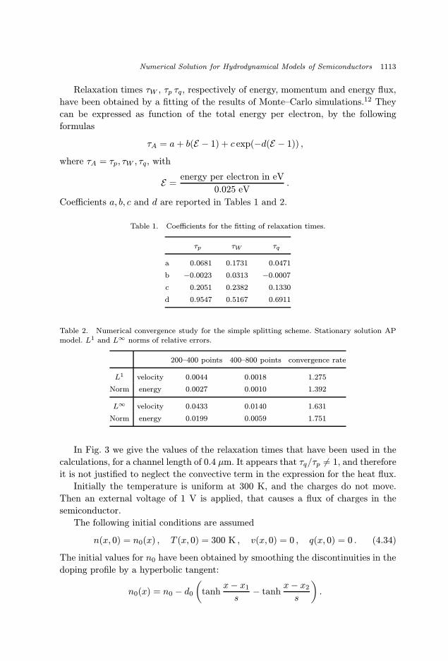
Relaxation times τW , τp τq, respectively of energy, momentum and energy flux,

have been obtained by a fitting of the results of Monte–Carlo simulations.12 They

can be expressed as function of the total energy per electron, by the following

formulas

τA = a+ b(E − 1) + c exp(−d(E − 1)) ,

where τA = τp, τW , τq, with

E =energy per electron in eV

0.025 eV.

Coefficients a, b, c and d are reported in Tables 1 and 2.

Table 1. Coefficients for the fitting of relaxation times.

τp τW τq

a 0.0681 0.1731 0.0471

b −0.0023 0.0313 −0.0007

c 0.2051 0.2382 0.1330

d 0.9547 0.5167 0.6911

Table 2. Numerical convergence study for the simple splitting scheme. Stationary solution AP

model. L1 and L∞ norms of relative errors.

200–400 points 400–800 points convergence rate

L1 velocity 0.0044 0.0018 1.275

Norm energy 0.0027 0.0010 1.392

L∞ velocity 0.0433 0.0140 1.631

Norm energy 0.0199 0.0059 1.751

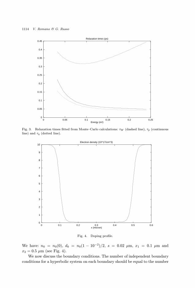
In Fig. 3 we give the values of the relaxation times that have been used in the

calculations, for a channel length of 0.4 µm. It appears that τq/τp 6= 1, and therefore

it is not justified to neglect the convective term in the expression for the heat flux.

Initially the temperature is uniform at 300 K, and the charges do not move.

Then an external voltage of 1 V is applied, that causes a flux of charges in the

semiconductor.

The following initial conditions are assumed

n(x, 0) = n0(x) , T (x, 0) = 300 K , v(x, 0) = 0 , q(x, 0) = 0 . (4.34)

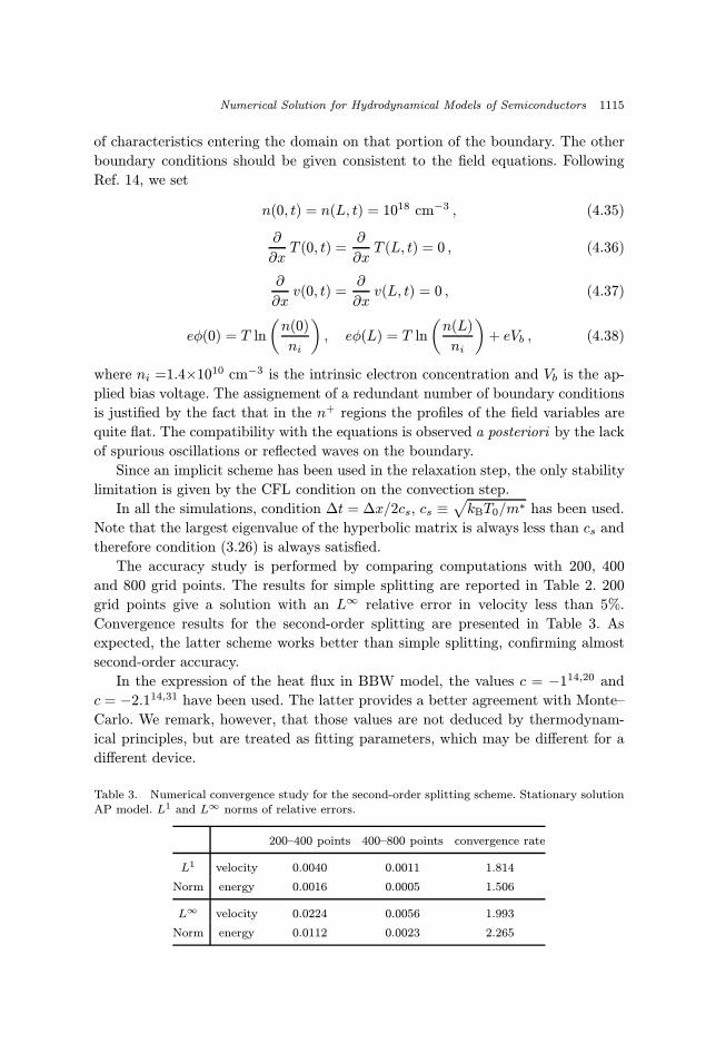
The initial values for n0 have been obtained by smoothing the discontinuities in the

doping profile by a hyperbolic tangent:

n0(x) = n0 − d0

(tanh

x− x1

s− tanh

x− x2

s

).

August 23, 2000 11:26 WSPC/103-M3AS 00055


0

0.05

0.1

0.15

0.2

0.25

0.3

0.35

0.4

0.45

0 0.05 0.1 0.15 0.2 0.25Energy (eV)

Relaxation times (ps)

Fig. 3. Relaxation times fitted from Monte–Carlo calculations: τW (dashed line), τp (continuousline) and τq (dotted line).

0

1

2

3

4

5

6

7

8

9

10

0 0.1 0.2 0.3 0.4 0.5 0.6x (micron)

Electron density (10^17/cm^3)

Fig. 4. Doping profile.

We have: n0 = n0(0), d0 = n0(1 − 10−2)/2, s = 0.02 µm, x1 = 0.1 µm and

x2 = 0.5 µm (see Fig. 4).

We now discuss the boundary conditions. The number of independent boundary

conditions for a hyperbolic system on each boundary should be equal to the number

August 23, 2000 11:26 WSPC/103-M3AS 00055


of characteristics entering the domain on that portion of the boundary. The other

boundary conditions should be given consistent to the field equations. Following

Ref. 14, we set

n(0, t) = n(L, t) = 1018 cm−3 , (4.35)

∂

∂xT (0, t) =

∂

∂xT (L, t) = 0 , (4.36)

∂

∂xv(0, t) =

∂

∂xv(L, t) = 0 , (4.37)

eφ(0) = T ln

(n(0)

ni

), eφ(L) = T ln

(n(L)

ni

)+ eVb , (4.38)

where ni =1.4×1010 cm−3 is the intrinsic electron concentration and Vb is the ap-

plied bias voltage. The assignement of a redundant number of boundary conditions

is justified by the fact that in the n+ regions the profiles of the field variables are

quite flat. The compatibility with the equations is observed a posteriori by the lack

of spurious oscillations or reflected waves on the boundary.

Since an implicit scheme has been used in the relaxation step, the only stability

limitation is given by the CFL condition on the convection step.

In all the simulations, condition ∆t = ∆x/2cs, cs ≡√kBT0/m∗ has been used.

Note that the largest eigenvalue of the hyperbolic matrix is always less than cs and

therefore condition (3.26) is always satisfied.

The accuracy study is performed by comparing computations with 200, 400

and 800 grid points. The results for simple splitting are reported in Table 2. 200

grid points give a solution with an L∞ relative error in velocity less than 5%.

Convergence results for the second-order splitting are presented in Table 3. As

expected, the latter scheme works better than simple splitting, confirming almost

second-order accuracy.

In the expression of the heat flux in BBW model, the values c = −114,20 and

c = −2.114,31 have been used. The latter provides a better agreement with Monte–

Carlo. We remark, however, that those values are not deduced by thermodynam-

ical principles, but are treated as fitting parameters, which may be different for a

different device.

Table 3. Numerical convergence study for the second-order splitting scheme. Stationary solutionAP model. L1 and L∞ norms of relative errors.

200–400 points 400–800 points convergence rate

L1 velocity 0.0040 0.0011 1.814

Norm energy 0.0016 0.0005 1.506

L∞ velocity 0.0224 0.0056 1.993

Norm energy 0.0112 0.0023 2.265

August 23, 2000 11:26 WSPC/103-M3AS 00055


01

23

45

0

0.1

0.2

0.3

0.4

0.5

−0.5

0

0.5

1

1.5

time (ps)

x (micron)

velo

city

(x

10^7

cm

/sec

)

Fig. 5. Time evolution of electron velocity for AP model. Second-order scheme with 200 points.

0

0.2

0.4

0.6

0.8

1

1.2

1.4

1.6

1.8

0 0.1 0.2 0.3 0.4 0.5 0.6x (micron)

Velocity (10^7 cm/s)

’AP’’MC’

’BBW (c=-1)’’BBW (c=-2.1)’

Fig. 6. Velocity profile (×107 cm/sec). AP model (continuous line), BBW model with c = −1.0(dashed line), c = −2.1 (dotted line) and with Monte–Carlo DAMOCLES code (squares). Thechannel length is 0.4 µm, and the applied voltage is 1 V.

In all our simulations, about five picoseconds are enough to reach steady state.

In Fig. 5 we report the time evolution of the velocity field. After a rapid transient,

steady state regime is approached.

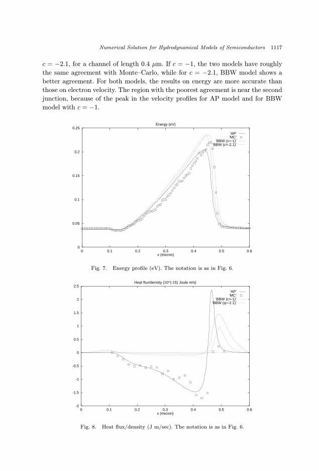
In Figs. 6 and 7 we compare velocity and energy profiles for Monte–Carlo results

obtained by the code DAMOCLES,11 and AP and BBW models for c = −1 and

August 23, 2000 11:26 WSPC/103-M3AS 00055


c = −2.1, for a channel of length 0.4 µm. If c = −1, the two models have roughly

the same agreement with Monte–Carlo, while for c = −2.1, BBW model shows a

better agreement. For both models, the results on energy are more accurate than

those on electron velocity. The region with the poorest agreement is near the second

junction, because of the peak in the velocity profiles for AP model and for BBW

model with c = −1.

0

0.05

0.1

0.15

0.2

0.25

0 0.1 0.2 0.3 0.4 0.5 0.6x (micron)

Energy (eV)

’AP’’MC’

’BBW (c=-1)’’BBW (c=-2.1)’

Fig. 7. Energy profile (eV). The notation is as in Fig. 6.

-2

-1.5

-1

-0.5

0

0.5

1

1.5

2

2.5

0 0.1 0.2 0.3 0.4 0.5 0.6x (micron)

Heat flux/density (10^(-15) Joule m/s)

’AP’’MC’

’BBW (c=-1)’’BBW (q=-2.1)’

Fig. 8. Heat flux/density (J m/sec). The notation is as in Fig. 6.

August 23, 2000 11:26 WSPC/103-M3AS 00055


-6e-06

-5e-06

-4e-06

-3e-06

-2e-06

-1e-06

0

1e-06

2e-06

0 0.1 0.2 0.3 0.4 0.5 0.6x (micron)

Electric field (Volt/m)

’AP’’BBW (c=-1)’

’BBW (c=-2.1)’

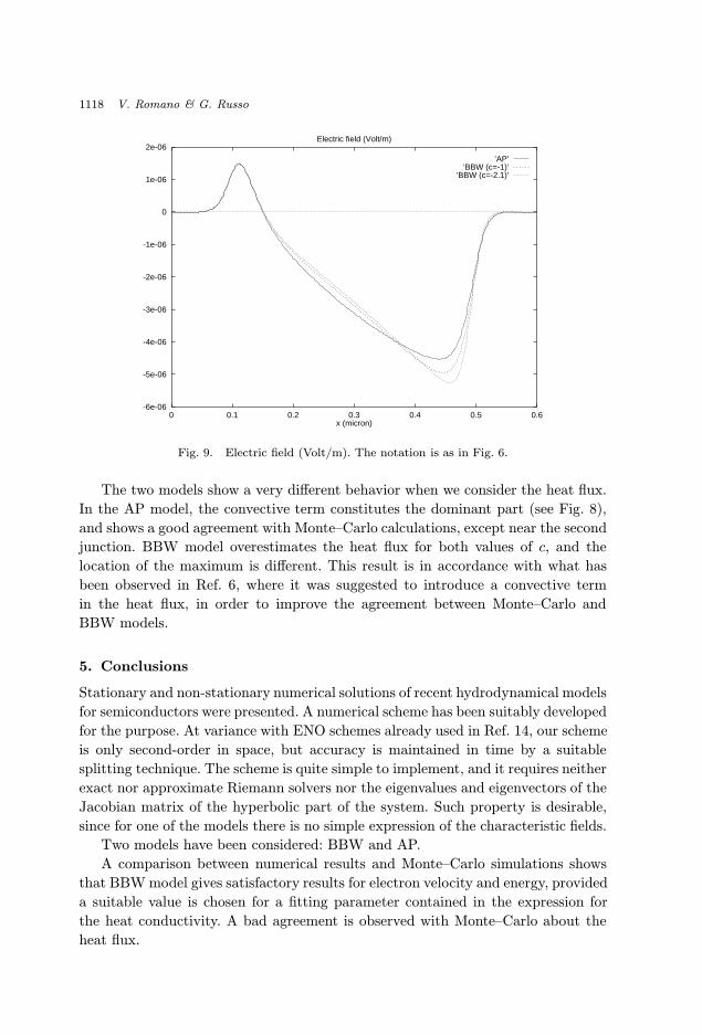
Fig. 9. Electric field (Volt/m). The notation is as in Fig. 6.

The two models show a very different behavior when we consider the heat flux.

In the AP model, the convective term constitutes the dominant part (see Fig. 8),

and shows a good agreement with Monte–Carlo calculations, except near the second

junction. BBW model overestimates the heat flux for both values of c, and the

location of the maximum is different. This result is in accordance with what has

been observed in Ref. 6, where it was suggested to introduce a convective term

in the heat flux, in order to improve the agreement between Monte–Carlo and

BBW models.

5. Conclusions

Stationary and non-stationary numerical solutions of recent hydrodynamical models

for semiconductors were presented. A numerical scheme has been suitably developed

for the purpose. At variance with ENO schemes already used in Ref. 14, our scheme

is only second-order in space, but accuracy is maintained in time by a suitable

splitting technique. The scheme is quite simple to implement, and it requires neither

exact nor approximate Riemann solvers nor the eigenvalues and eigenvectors of the

Jacobian matrix of the hyperbolic part of the system. Such property is desirable,

since for one of the models there is no simple expression of the characteristic fields.

Two models have been considered: BBW and AP.

A comparison between numerical results and Monte–Carlo simulations shows

that BBW model gives satisfactory results for electron velocity and energy, provided

a suitable value is chosen for a fitting parameter contained in the expression for

the heat conductivity. A bad agreement is observed with Monte–Carlo about the

heat flux.

August 23, 2000 11:26 WSPC/103-M3AS 00055


AP model, on the contrary, is derived in a systematic way from a kinetic formu-

lation, by using techniques proper of extended thermodynamics. The model gives

a reasonable agreement with Monte–Carlo for the heat flux, but the agreement of

velocity and energy profiles is similar to that obtained by BBW model with c = −1.

Therefore, although AP model gives a better description of the heat flux, it is

not yet satisfactory. We believe that the theoretical foundation of the AP model is

physically sound, but the modelling of the production terms needs to be improved.

A possible way is to derive the constitutive functions by employing Levermore’s

theory23 or the maximum entropy principle9 which allow one to get closure relations

also for the production terms. This could avoid to resort to a fitting of the relaxation

times and to lead to a model without free parameters, valid for a general class of

electron devices.

Acknowledgments

The authors would like to thank Prof. A. M. Anile for helpful discussion and

Dr. O. Muscato who provided the results of the Monte–Carlo simulations obtained

by DAMOCLES.

This work has been partially supported by MURST, by CNR project Modelli

matematici per semiconduttori. Progetto speciale: metodi matematici in fluidod-

inamica e dinamica molecolare, grant # 96.03855.CT01, and by TMR program

Asymptotic methods in kinetic theory, grant # ERBFMRXCT970157.

References

1. W. Haensch, The Drift-Diffusion Equation and Its Application in MOSFETModeling (Springer-Verlag, 1991).

2. P. A. Markowich, C. A. Ringhofer and C. Schmeiser, Semiconductor Equations(Springer-Verlag, 1990).

3. S. Chapman and T. G. Cowling, The Mathematical Theory of NonuniformGases (Cambridge Univ. Press, 1970), 3rd ed.

4. K. Blotekjaer, Transport equation for electrons in two-valley semiconductors, IEEETrans. Electron Devices ED-17 (1970) 38–47.

5. G. Baccarani and M. R. Wordeman, An investigation on steady-state velocity over-shoot in Silicon, Solid-State Electronics 29 (1982) 970–977.

6. M. A. Stettler, M. A. Alam and M. S. Lundstrom, A critical examination of theassumption underlying macroscopic transport equation for silicon device, IEEE Trans.Electron Devices 40 (1993) 733–739.

7. S.-C. Lee and T.-W. Tang, Transport coefficients for a silicon hydrodynamical modelextract from inhomogeneous Monte–Carlo simulation solid-state electronics 35 (1992)561–569.

8. A. M. Anile and S. Pennisi, Thermodynamic derivation of the hydrodynamical modelfor charge transport in semiconductors, Phys. Rev. B46 (1992) 13186–13193.

9. I. Muller and T. Ruggeri, Extended Thermodynamics (Springer-Verlag, 1993).10. D. Jou, J. Casas-Vazquez and G. Lebon, Extended Irreversible Thermodynam-

ics (Springer-Verlag, 1993).

August 23, 2000 11:26 WSPC/103-M3AS 00055


11. M. V. Fischetti and S. Laux, Phys. Monte Carlo study of electron transport in siliconinversion layers, Phys. Rev. B48 (1993) 2244–2274.

12. O. Muscato, R. M. Pidatella and M. V. Fischetti, Monte Carlo and hydrodynamicssimulation of a one dimensional n+–n–n+ silicon diode, Electronics VLSI Design 6(1998) 247–250.

13. H. Nessyahu and E. Tadmor, Non-oscillatory central differencing for hyperbolicconservation law, J. Comput. Phys. 87 (1990) 408–463.

14. E. Fatemi, J. Jerome and S. Osher, Solution of hydrodynamic device model usinghigh-order nonoscillatory shock capturing algorithms, IEEE Trans. Computer-AidedDesign 10 (1991) 232–398.

15. A. Anile, V. Romano and G. Russo, Extended hydrodynamical model of carrier trans-port in semiconductors, SIAM J. Appl. Math., to appear.

16. N. C. Ashcroft and N. D. Mermin, Solid State Physics (Holt-Sounders, 1976).17. N. Ben Abdallah, P. Degond and S. Genieys, An energy-transport model for semicon-

ductors derived from the Boltzmann equation, J. Stat. Phys. 84 (1996) 205–231.18. N. Ben Abdallah and P. Degond, On a hierarchy of macroscopic models for semicon-

ductors, J. Math. Phys. 37 (1996) 3306–3333.19. C. L. Gardner, J. W. Jerome and D. J. Rose, Numerical methods for the hydrodynamic

device model: subsonic flow, IEEE Trans. Computer-Aided Design 8 (1989) 501–507.20. C. L. Gardner, Numerical simulation of a steady-state electron shock wave in a sub-

micrometer semiconductor device, IEEE Trans. Electron Devices 38 (1991) 392–398.21. A. M. Anile and O. Muscato, Improved hydrodynamical model for carrier transport in

semiconductors, Phys. Rev. B51 (1995) 16728–16740.22. S. R. de Groot and P. Mazur, Nonequilibrium Thermodynamics (Dover, 1985).23. C. D. Levermore, Moment Closure Hierarchies for Kinetic Theories, J. Stat. Phys.

83 (1996) 331–407.24. C. Truesdell and R. G. Muncaster, Fundamentals of Maxwell’s Kinetic Theory

of a Simple Monoatomic Gas (Academic Press, 1980).25. R. LeVeque, Numerical Methods for Conservation Laws (Birkhauser, 1990).26. B. Van Leer, Towards the ultimate conservative difference scheme V. A second-order

sequel to Godunov’s method, J. Comput. Phys. 32 (1979) 101–136.27. A. Harten and S. Osher, Uniformily high-order accurate non-oscillatory schemes,

SIAM J. Numer. Anal. 24 (1987) 279–309.28. R. E. Caflisch, G. Russo and Shi Jin, Uniformly accurate schemes for hyperbolic

systems with relaxation, SIAM J. Numer. Anal. 34 (1) (1997) 246–281.29. F. Liotta, V. Romano and G. Russo, Central schemes for system of balance laws,

Internat. Series Numer. Math. 130 (1999) 651–660.30. T. Vogelsang and W. Haensch, A novel approach for including band structure effects

in a Monte Carlo simulation of electron transport in silicon, J. Appl. Phys. 70 (1991)1493–1499.

31. A. Gnudi, F. Odeh and M. Rudan, Investigation of non-local transport phenomena insmall semiconductor devices, Euro. J. Telecom. 1 (1990) 307–312.

numerical solution for hydrodynamical models of … · cron devices, and several relevant physical...

Documents