numerical simulation of the blast impact problem …

NUMERICAL SIMULATION OF THE

BLAST IMPACT PROBLEM USING THE

DIRECT SIMULATION MONTE CARLO

(DSMC) METHOD

Anupam Sharma 1 and Lyle N. Long 2

Department of Aerospace Engineering,233 Hammond Building

University Park, PA - 16802

Abstract

A particle approach using the Direct Simulation Monte Carlo (DSMC) method isused to solve the problem of blast impact with structures. A novel approach tomodel the solid boundary condition for particle methods is presented. The solveris validated against an analytical solution of the Riemann shocktube problem andagainst experiments on interaction of a planar shock with a square cavity. Blastimpact simulations are performed for two model shapes, a box and an I-shapedbeam, assuming that the solid body does not deform. The solver uses domain de-composition technique to run in parallel. The parallel performance of the solver ontwo Beowulf clusters is also presented.

Key words: Direct Simulation Monte Carlo (DSMC), Blast Impact, ObjectOriented Programming (OOP)

1 Introduction

The protection of civilians and military personnel from an attack by anothercountry or by terrorists is of primary importance for a nation. In recent timesof heightened terrorist activities and alarming threats of future attacks, it hasbecome utmost important to develop safe housing and barracks respectively

Email address: [email protected] (Lyle N. Long).1 Graduate Research Assistant, Aerospace Engineering2 Professor, Aerospace Engineering

Preprint submitted to Elsevier Science 1 April 2004

for innocent civilians and military personnel. This problem requires the sci-entific community to research the general area of design and development ofprotective structures. Recent tragic mishaps such as the attacks on the WorldTrade Center and the USS Cole have brought this problem to the foreground.

Research in this area has been ongoing for several years but has been focusedprimarily on open-air, field blasts. Such experiments involve detonation of realexplosives and investigation of the impact of the explosion on nearby struc-tures constructed specifically for this purpose. These experiments are bothhazardous and expensive. Also, such large-scale experiments involving sub-stantial amount of explosives can only be performed by the military becauseof the federal regulations.

A different approach to the problem is to use computers to simulate the im-pact of a blast wave generated from an explosion with solid structures. Thisapproach is more feasible for universities and other private research groupsand is free of hazards associated with the handling of explosives.

This study focuses on numerical simulations of the interaction of blast waveswith structures and the prediction of resulting pressure loading. This is alsoknown as the “load definition” problem. The pressure loading may then beused as an input to a commercially available structural dynamics solver, suchas ANSYS to determine if the structure would fail in such circumstances.In this manner the structural mechanics problem (of solving the strain anddeformation) is uncoupled from the fluid dynamics problem (of predicting thepressure / stress loading). The uncoupled fluid dynamics problem is solvedassuming that the structure does not deform because of the impact. Hence, theassumption of uncoupling is only accurate if the structure remains intact. Oncethe structure deforms it will alter the blast wave and the two problems willbecome coupled. In the present study we are dealing only with the uncoupledproblem.

The key requirements of a numerical solver for this problem are:

• It should be able to handle complicated geometries such as buildings (forexternal blasts), and cubicles and rooms (for internal blasts).

• This mission is time critical and hence the simulations should be relativelyfast. One cannot afford to spend months on a single simulation. The speedalso determines the cost of the computation. The faster the results areobtained, the more economical it is.

• Since the goal is to design for threats that cannot be accurately determined,slight inaccuracy in the results is acceptable if it significantly reduces theturnaround time.

The Direct Simulation Monte Carlo (DSMC) method meets the above con-ditions and is chosen for the study. The following section discusses in detail

2

the advantages of DSMC over conventional Computational Fluid Dynamics(CFD) methods for the problem of interest.

A parallel, object oriented DSMC solver is developed for this problem. Thesolver is written in C++ and is designed using the object oriented featuresof the language. The parallelization is achieved by domain decomposition andusing the Message Passing Interface (MPI) library for inter-processor commu-nications. There are two reasons for making the code parallel: firstly, to solvelarge-size problems, and secondly, to reduce the turnaround time.

In the following sections the implementation of the solid and inflow bound-ary conditions, and diatomic gas modeling are described. The object orientedapproach for the solver and the parallelization technique are also discussed.The solver is verified against the analytical solution of the Riemann shocktubeproblem. The solid and inflow boundary conditions are separately validatedagainst analytical results. The problem of a normal shock interaction with asquare cavity is simulated and compared against the experiments by Igra etal. [1]. Two model shapes, a box and a I-shaped beam are studied for blastimpact.

2 DSMC

The Direct Simulation Monte Carlo (DSMC) method has gained a lot of pop-ularity since its development by Bird [2] in the 1960s. The method has beenthoroughly tested for high Knudsen-number (> 0.2) flows over the past 25years and found to be in excellent agreement with both experimental data [3]and Molecular-Dynamics computations [4]. The method was developed pri-marily for aerospace applications in rarefied gas dynamics and has been exten-sively applied in that area [3,5,6,7,8]. DSMC has also been successfully usedfor hypersonic flows [6,9,10] and modeling detonations [11]. In fact, DSMChas become, de facto, the principal tool to investigate high Knudsen numberflows. DSMC is also very useful for modeling flows involving chemical reac-tions [12,13,14,15].

DSMC is a direct particle simulation method based on the kinetic theory ofgases. The fundamental idea is to track a large number of statistically repre-sentative particles. The particles move according to Newton’s laws and collidewith each other conserving mass, momentum and energy. The particles’ mo-tion is calculated deterministically but the collisions are treated statistically.The direction of a molecule’s post-collision velocity is calculated by performingrandom walks (a random process consisting of a sequence of discrete steps offixed length) while conserving momentum and energy. Hence, the collisions inDSMC are only statistically correct. The treatment of intermolecular collisions

3

Start

Sort into cells

Collide

Sample resultsOutput

t/ts = 0If

t > totaltime

If

Apply BCsMove Particles

No

No

Yes

Main loop

Cells & ParticlesInitialize

Average runs forunsteady flow

oraverage samples

StopYes

For unsteady flow,repeat until reqd.sample is obtained

Read data

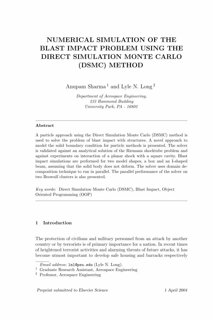
Fig. 1. A Flowchart of a typical DSMC simulation.

is the key difference between Molecular Dynamics and DSMC. In the Molecu-lar Dynamics method the particle interactions are calculated using potentialssuch as the Lennard-Jones potential.

Figure 1 is a flowchart of a typical DSMC simulation. There are essentially fourroutines in a DSMC simulation: (a) move the particles for time ∆t assuming nointermolecular collisions but treat the collisions with the domain boundaries,(b) sort the particles in different cells, (c) perform intermolecular collisions,and (d) sample macroscopic properties of interest.

DSMC simulations become more exact as the time step and the cell size tendto zero. Wagner [16] has proved that the DSMC method converges to thesolution of the Boltzmann equation in the limit of the time step and the cellsize equal to zero. Since the motion of the particles is independent of thecell structure, the disturbances can propagate at the sound or shock wavespeed even when the ratio of cell size to the time step is relatively very small.Therefore, DSMC is not limited by a stability criterion such as the Courant-Fredrichs-Lewy (CFL) condition.

There have been few attempts [17,18] to use DSMC for continuum problems(Kn < 0.1). This is because DSMC inherently assumes that the cell size andthe time step in a simulation are of the order of magnitude of the mean freepath and the mean collision time respectively of the gas. Typical magnitudes

4

of the mean free path and the mean collision time of air in standard atmo-spheric conditions are of the order 10−8 m and 10−10 seconds respectively. Asimulation of flow over large bodies (typical length O(m)) in such conditionsrequires enormous time and memory. But, in a rarefied atmosphere, the valuesof the mean free path and the mean collision time can be quite large. Thismakes possible the simulation of flows over re-entry vehicles using DSMC inreasonable time. When the body of interest is comparable to the size of themean free path, e.g., in micro-devices, DSMC can also be inexpensively usedat standard atmospheric conditions.

Pullin [17] suggested an algorithm to extend the application of DSMC to thecontinuum regime for inviscid, perfect-gas flows. The assumption of perfect-gas inviscid flow is equivalent to assuming local thermal equilibrium (Kn = 0)at every point and at all times [17]. This is analogous to solving the Eulerequations. In his algorithm, Pullin reinitializes the velocity of every moleculeto the local Maxwellian after every iteration thus insuring local equilibrium.Pullin [17] suggested that for such idealized cases, the cell size and the timestep could be chosen to be a practically infinite number of times of the molec-ular mean free path and the mean collision time since the fluid properties areassumed to be constant over each cell. The error in making such an approxi-mation is that the flow properties are smeared over a cell width. For example,if we simulate a shock wave, the minimum thickness of the wave by a DSMCsimulation will be equal to the cell size.

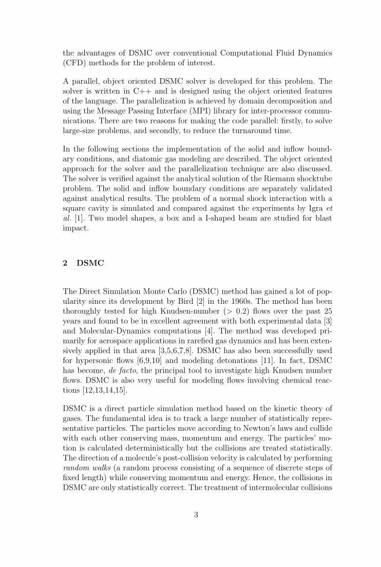
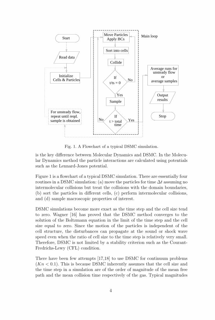
Interestingly, Pullin [17] ruled out the possibility of using his approach becauseof the time penalty associated with the calculation of equilibrium molecularvelocities at each time step. Recently, Sharma and Long [19] have proposedan inexpensive procedure to achieve local thermodynamic equilibrium. In thisprocedure, one allows enough collisions per cell per time step to relax the gasto the local Maxwellian. The maximum number of collisions is a function ofthe number of particles in the cell but we fix it to about three-fourths of thatnumber. This is a conservative approximate as can be inferred from Figs. 2and 3. These figures plot the results of a simple experiment of rotationalrelaxation in air. The gas is initially perturbed from Maxwellian by assigningzero rotational temperature. Figure 2 plots the rotational and translationaltemperatures as a function of number of collisions for three different numbersof particles per cell. After a sufficient number of collisions, the gas returns tothe local Maxwellian. This limit increases with increasing number of particles,but is always less that three-fourths the value as can be seen from Fig. 3.

In order to do one collision, approximately 60 floating point operations arerequired as opposed to about 360 required to assign a Maxwellian velocity toone particle. Hence, the procedure of relaxing the gas to a Maxwellian usingcollisions is at least about six times more economical. A significant reductionin the computation time by this procedure makes DSMC a practical Euler

5

T rot

T tr

0

50

100

200

250

300

0 10 20 30 40 50 60

T (

K)

Number of collisions

Number of particles per cell = 50

100150

150

Fig. 2. Rotational relaxation in air.

0

200

400

600

800

1000

1200

1400

1600

0 500 1000 1500 2000

Num

ber

of c

ollis

ions

req

uire

d fo

r 1%

err

or

Number of particles per cell

3/4 x #partobserved

Fig. 3. Minimum number of collisions per cell per time step required to reduce thedifference between rotational and translational temperatures to within 1%.

solver.

It is essentially the robustness of DSMC that has made this method widelypopular. Research is going on to apply this method to other areas such asacoustics [20,21]. The interested reader is referred to Bird [6] for detaileddescription of DSMC and its applications.

6

3 DSMC Solver

A parallel, object oriented DSMC solver is developed to study blast wavestructure interactions. A uniform, Cartesian grid is used with embedded sur-faces to model complex geometries. The particles are distributed uniformlyacross the domain and their velocities are given by a Maxwellian distributionat the start of each run. All the particles inside the solid body (closed surface)are removed. This is done to avoid any information exchange into the solidbody because of intermolecular collision.

The implementation of different aspects of the solver are described in thefollowing subsections.

3.1 Solid Boundary Condition

The ultimate goal of a blast-impact simulation is to couple the shock-wavesimulation with a structural dynamics model. This would allow simultaneousdeformation of the solid body in the simulation as the stress on the bodyexceeds the yield stress. Although the solid body is not allowed to deform inthis study, a very general approach to model the solid boundary is developed.This will allow the same code to be used with little modification when thebody is simultaneously deformed.

Since we are only interested in Euler calculations, inviscid boundary condi-tions are imposed on the solid surfaces. Inviscid boundary condition in thesolver is implemented by imposing specular reflection of the particles whenthey hit a solid surface. The solid surfaces are made of triangular patches toincorporate arbitrary-shaped bodies. The patches may be arbitrarily orientedin 3-dimensions and the particles are also moving in a 3-dimensional space. Weneed to find the post-collision position and velocity of the particles reflectedoff the solid surface. The probability of a collision of a particle with a giventriangle is very small and therefore it is imperative to devise a computationallyefficient algorithm to reject the particles that do not collide with the triangle.

A quick way to eliminate the particles which will definitely not collide withthe solid body is by checking if the particle crosses into a box bounding thesolid body. It is much cheaper to check the intersection with a bounding box(a cuboid) than an arbitrary solid body since it only requires six logical state-ments in a subroutine to compare the three Cartesian coordinates (position)with the dimensions of the box. An easy way to implement this is by using theSutherland line clipping algorithm [22] in three dimensions. This algorithm iswidely used in polygon clipping in computer graphics applications. The idea isto have an efficient way to ignore the line segments that lie completely outside

7

c

c

c

LTRB

L − leftT − topR − rightB − bottom

00001000

1100 0100 0110

0010

001100011001

LEFT

TOP

RIGHT

BOTTOM

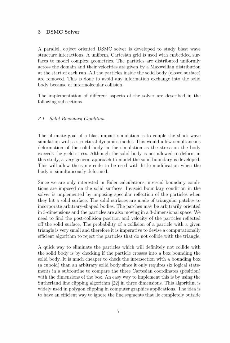
Fig. 4. Sutherland line clipping algorithm for a 2-D case. The lines marked with c©should be clipped.

the canvas. If we extend the canvas to 3 dimensions, we get a box and insteadof 2-D line segments we can deal with 3D line segments. Correlating line seg-ments with the motion of particles in one time step, and the 3D box with abox bounding our solid object, we can directly use the Sutherland algorithmfor our problem.

Figure 4 illustrates the Sutherland algorithm in 2D. The 2D space is dividedby the square (canvas) into 4 regions with respect to the canvas - LEFT, TOP,RIGHT and BOTTOM. Each point in the 2D space can now be located byusing a binary representation in four bits one each for LEFT, TOP, RIGHTand BOTTOM. The appropriate bits are turned on depending on the locationof the point (i.e. if the point is to the left and top of the square then the LEFTand TOP bits are 1 and the rest are 0). It is intuitive that if we get a nonzerovalue when we perform an “AND” operation on the binary representation ofthe end points of a line segment, the segment will never intersect the canvas.

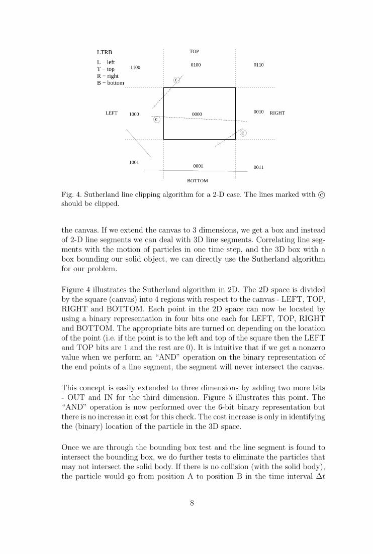
This concept is easily extended to three dimensions by adding two more bits- OUT and IN for the third dimension. Figure 5 illustrates this point. The“AND” operation is now performed over the 6-bit binary representation butthere is no increase in cost for this check. The cost increase is only in identifyingthe (binary) location of the particle in the 3D space.

Once we are through the bounding box test and the line segment is found tointersect the bounding box, we do further tests to eliminate the particles thatmay not intersect the solid body. If there is no collision (with the solid body),the particle would go from position A to position B in the time interval ∆t

8

L − leftT− topR−rightB−bottom

O − outI − in

B=1

R=1

O=1

T=1

L=1

I=1

O I L T R B

Fig. 5. Sutherland line clipping algorithm extended to 3 dimensions.

12

3

A

B�

XC

XI

Bn̂

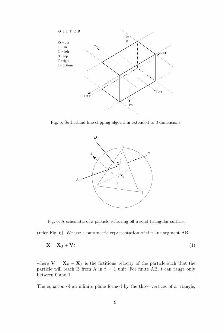
Fig. 6. A schematic of a particle reflecting off a solid triangular surface.

(refer Fig. 6). We use a parametric representation of the line segment AB.

X = XA + Vt (1)

where V = XB − XA is the fictitious velocity of the particle such that theparticle will reach B from A in t = 1 unit. For finite AB, t can range onlybetween 0 and 1.

The equation of an infinite plane formed by the three vertices of a triangle,

9

X1,X2 and X3 is

(X−X1).n̂ = 0 (2)

where, X is the vector defining the plane and n̂ is a unit normal to the planecalculated using Eq. 3.

n̂ =(X1 −X2)× (X3 −X2)

|(X1 −X2)× (X3 −X2)|(3)

Note that the normal to the plane need not be calculated at every time step.It may be calculated during the first iteration and stored for the rest of thesimulation. The intersection point, XI of the segment with the infinite planecan be obtained by simultaneously solving Eqs. 4 and 5 for t∗ and XI .

(XI −X1).n̂ = 0 (4)

XI = XA + Vt∗ (5)

The solution of the above equations is

t∗ =(XA −X1).n̂

V.n̂(6)

and XI may be obtained from Eq. 5 using t∗ from Eq. 6. The finite segment,AB intersects the infinite plane only if 0 ≤ t∗ ≤ 1 The equality on eitherside meaning that XI is the same as XA or XB. If t∗ does not satisfy theabove condition, then we can say that the particle will not hit the triangle. If,however, t∗ satisfies the above condition then we need to find out if XI liesinside the triangle.

A quick elimination of a number of particles not intersecting the triangle maybe performed by checking if XI lies outside a circle enclosing the triangle.An obvious choice for this is the circumcircle, but we do not choose the cir-cumcircle because it is computationally involving to obtain the center of acircumcircle in three dimensions. We choose a circle with a radius, r = 2/3×the largest edge of the triangle, and its center at the centroid. This circle willcompletely enclose the triangle but will not exactly circumscribe it. The rea-soning behind this is - the vertex of a triangle farthest from its centroid is ata distance of 2/3× the maximum of the three medians. Since the largest edgeof a triangle is always greater than the largest median, the circle with radius rand center at the centroid of the triangle will completely enclose the triangle.

We calculate the centroid of the triangle and the radius of the enclosing circledescribed above during the first iteration. All XIs with |XI −XC | > r will hit

10

XI

XI inside the triangle XI outside the triangle

21

3

12

3

r

XI

pq q p

r

cc

c

c

c

ac

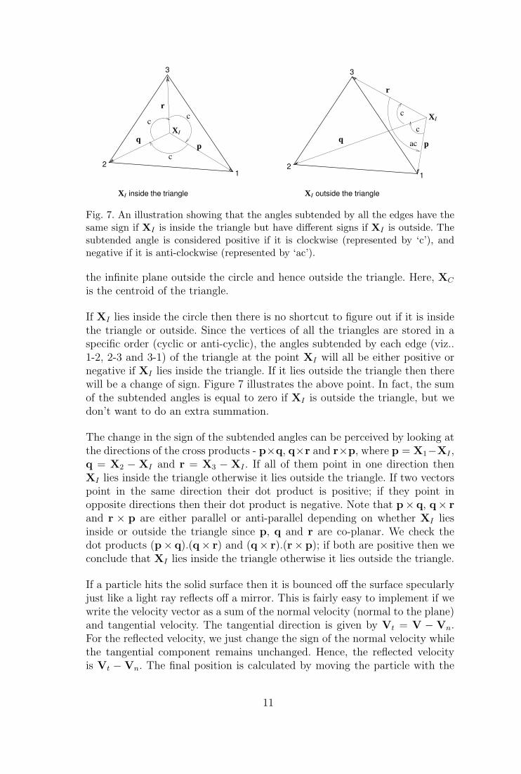
Fig. 7. An illustration showing that the angles subtended by all the edges have thesame sign if XI is inside the triangle but have different signs if XI is outside. Thesubtended angle is considered positive if it is clockwise (represented by ‘c’), andnegative if it is anti-clockwise (represented by ‘ac’).

the infinite plane outside the circle and hence outside the triangle. Here, XC

is the centroid of the triangle.

If XI lies inside the circle then there is no shortcut to figure out if it is insidethe triangle or outside. Since the vertices of all the triangles are stored in aspecific order (cyclic or anti-cyclic), the angles subtended by each edge (viz..1-2, 2-3 and 3-1) of the triangle at the point XI will all be either positive ornegative if XI lies inside the triangle. If it lies outside the triangle then therewill be a change of sign. Figure 7 illustrates the above point. In fact, the sumof the subtended angles is equal to zero if XI is outside the triangle, but wedon’t want to do an extra summation.

The change in the sign of the subtended angles can be perceived by looking atthe directions of the cross products - p×q, q×r and r×p, where p = X1−XI ,q = X2 − XI and r = X3 − XI . If all of them point in one direction thenXI lies inside the triangle otherwise it lies outside the triangle. If two vectorspoint in the same direction their dot product is positive; if they point inopposite directions then their dot product is negative. Note that p× q, q× rand r × p are either parallel or anti-parallel depending on whether XI liesinside or outside the triangle since p, q and r are co-planar. We check thedot products (p× q).(q× r) and (q× r).(r× p); if both are positive then weconclude that XI lies inside the triangle otherwise it lies outside the triangle.

If a particle hits the solid surface then it is bounced off the surface specularlyjust like a light ray reflects off a mirror. This is fairly easy to implement if wewrite the velocity vector as a sum of the normal velocity (normal to the plane)and tangential velocity. The tangential direction is given by Vt = V − Vn.For the reflected velocity, we just change the sign of the normal velocity whilethe tangential component remains unchanged. Hence, the reflected velocityis Vt −Vn. The final position is calculated by moving the particle with the

11

reflected velocity for the remaining time taking into consideration that theremight be further collisions if the solid body is concave.

The solid boundary condition implementation is summarized in a step-by-stepprocedure below:

(1) Ignore all particles that lie outside the bounding box. These are foundusing the Sutherland algorithm.

(2) For each particle, calculate the intersection of its trajectory with the infi-nite planes formed by each triangle of the solid body. Ignore the particlesthat do not intersect with any of the planes.

(3) Ignore the collision if the intersection point (found in step 2) lies outsidea circle that encloses the corresponding triangle.

(4) Check if the intersection point lies inside the triangle. If yes, then themolecule collides with the solid body and is reflected back specularlyfrom the surface.

3.2 Inflow Boundary Condition

An inflow boundary condition is used for shocktube type simulations where aplanar shockwave is desired. For a specified shock strength and atmosphericconditions ahead of the shock wave, the conditions behind the shock wave maybe calculated by using normal shock relations (c.f., ref. [23]). The velocity,density and temperature behind the shock wave are then applied at the inflowboundary. This approach can be used with conventional CFD schemes as wellas with particle methods such as DSMC.

The treatment of the inflow boundary condition in DSMC is different than inthe CFD schemes. This is because, in conventional CFD schemes, the bound-ary condition is known in terms of flow variables whereas in DSMC we needthe number, position and velocity of the entering particles. A simple way toimplement the inflow boundary condition is to delete all the particles that goout of the inflow boundary and those that are in the first layer of cells nearthe boundary at each time step. The correct number of particles (obtained bydividing the density by the product of the volume of a cell and the ratio of realto simulated particles) are then inserted in each cell in this layer. These aredistributed uniformly as we assume local thermodynamic equilibrium at theboundary. The velocities of these particles are obtained using a Maxwelliandistribution based on the inflow velocity and temperature calculated usingnormal shock relations.

12

3.3 Model for Diatomic Gases

The air is considered to be essentially a diatomic gas. The DSMC solver is re-quired to model the diatomic nature of a gas as the present study concentrateson shock waves propagating through air. A diatomic molecule has five degreesof freedom while a monoatomic molecule has only three degrees of freedom.The additional degrees of freedom are from the rotation of molecules abouttheir center of mass. The rotation allows for additional storage of energy inthe molecule, namely, the rotational kinetic energy. Vibrational modes are notincluded here.

A monatomic gas may be represented by hard spheres. However, an internalenergy model is required to truly represent a diatomic gas. Such a model isrequired to incorporate the internal energy associated with the rotation ofthe molecule. It is important to note that our only concern is to handle theinternal energy exchange between the molecules during the collisions; we arenot worried about the structure of the molecule and how the collisions actuallyoccur considering the structure of the molecules.

Larsen and Borgnakke [24] model a diatomic molecule as a sphere with a vari-able internal energy. The internal energy and the translational energy of thecolliding molecules are redistributed during the collision but the total energyis conserved. This is a phenomenological model which may be used for poly-atomic gases with multiple degrees of freedom. The following mathematicallydescribes the model for a diatomic gas.

The internal energy of each molecule is initialized to be ei = mRTr where mis the mass of the molecule, R is the gas constant and Tr is the rotationaltemperature. Tr is initially the same as the total temperature since the gasis in thermal equilibrium. Note again that each molecule is diatomic but it isconsidered to be spherical for calculating the collision frequency. The internalenergy is considered only when the energy is redistributed during the collisionprocess.

Two molecules are randomly chosen from a cell to be considered for collision.Let us name these molecules a and b for referencing. The relative velocity ofthe molecules is calculated as gab = ub − ua. The collision pair (a, b) is thenaccepted if the following is satisfied.

g(ν−5)/(ν−1)ab /[g

(ν−5)/(ν−1)ab ]max > R1 (7)

where,R1 is a random number from the seriesR1,R2, . . . having a rectangulardistribution in [0; 1]. ν = ∞ for a hard sphere molecule which reduces theabove expression to gab/[gab]max > R1. Random pairs are chosen until the

13

above condition is satisfied.

Once a pair satisfies the inequality in Eq. 7, the total energy of the moleculese = et + ei is calculated. The translational energy is et = 1

2µg2

ab where µ =mamb/(ma +mb) is the reduced mass, and the internal energy is ei = eia + eib .

The ratio of the probability to the maximum probability of a particular valueof the translational energy for a diatomic molecule is

P/Pmax = 4(et/e)(1− et/e) (8)

Two sets of random numbers (R2,R3) are drawn until the following inequalityis satisfied.

{P/Pmax = 4(R2)(1−R2)} ≥ R3

The post-collision kinetic energy, e′t = R2e and the internal energy e′i = e− e′t(conservation of energy) are then redistributed between the two molecules.The internal energy is divided randomly: e′ia = R4e

′i and e′ib = e′i − e′ia . The

post-collision velocities of the molecules are obtained in the same manner as inthe case of hard sphere molecules with an updated relative velocity magnitude,

gab =√

2e′t/µ.

We use this model because of its simplicity and generality. It is easy to programand still gives excellent results.

3.4 Object-Oriented Approach

An Object-Oriented (OO) approach is used in the development of a DSMCsolver for this study. It is most suitable for a particle method solver such asDSMC because the particles and cells are physical objects that have a definedset of attributes and functions. There are, of course, other benefits of using anobject-oriented approach, namely, the code is reusable, easy to maintain andmore organized.

The different classes used in the solver and their relationships are shown by aUnified Modeling Language (UML) diagram in Fig. 8. A very natural choice ofclasses is adopted: The particle class defines the properties and the actions ofa particle. Since the selection of collision pairs and the sampling of propertiesare performed using only the particles in each cell, a cell class is defined.

The solver itself is a class which is derived from an abstract generic solver.The abstract solver simply provides the declaration of the required actions

14

CGenericSolver

CSolidSurface

CParallelSolver

CMpiWrap

CCell

CParticle

CExcptn

CBox

CSurfaceElement

1..1

1..1

1..1 1..1

1..1

1..n

1..n

1..n

1..1

1..n

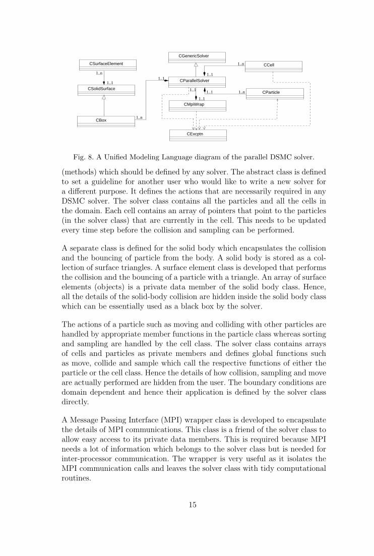
Fig. 8. A Unified Modeling Language diagram of the parallel DSMC solver.

(methods) which should be defined by any solver. The abstract class is definedto set a guideline for another user who would like to write a new solver fora different purpose. It defines the actions that are necessarily required in anyDSMC solver. The solver class contains all the particles and all the cells inthe domain. Each cell contains an array of pointers that point to the particles(in the solver class) that are currently in the cell. This needs to be updatedevery time step before the collision and sampling can be performed.

A separate class is defined for the solid body which encapsulates the collisionand the bouncing of particle from the body. A solid body is stored as a col-lection of surface triangles. A surface element class is developed that performsthe collision and the bouncing of a particle with a triangle. An array of surfaceelements (objects) is a private data member of the solid body class. Hence,all the details of the solid-body collision are hidden inside the solid body classwhich can be essentially used as a black box by the solver.

The actions of a particle such as moving and colliding with other particles arehandled by appropriate member functions in the particle class whereas sortingand sampling are handled by the cell class. The solver class contains arraysof cells and particles as private members and defines global functions suchas move, collide and sample which call the respective functions of either theparticle or the cell class. Hence the details of how collision, sampling and moveare actually performed are hidden from the user. The boundary conditions aredomain dependent and hence their application is defined by the solver classdirectly.

A Message Passing Interface (MPI) wrapper class is developed to encapsulatethe details of MPI communications. This class is a friend of the solver class toallow easy access to its private data members. This is required because MPIneeds a lot of information which belongs to the solver class but is needed forinter-processor communication. The wrapper is very useful as it isolates theMPI communication calls and leaves the solver class with tidy computationalroutines.

15

It is extremely important to provide a safe exit mechanism to handle excep-tional situations in a parallel program. If a runtime error develops and thereis no rectification possible then all the processors running the job need to benotified to abort the job and release the computer resources they were using.An exception class is developed to deal with such situations. All the classescan throw an object of this class as an exception at any point during theprogram execution. The exception is caught in the MPI wrapper class whichsafely aborts the parallel program and generates a log of the error. The use ofexceptions makes the code more robust.

The C++ solver prepared using these classes is well organized, easy to readand use, maintainable and adaptable for specific problems. It is also well doc-umented using standard doc++ [25] comments.

3.5 Parallelization

There are two main reasons why a parallel DSMC solver is desired: (1) Thesize of the problem may easily become larger than the available memory ofa machine, so there is a memory constraint, and (2) a quick solution to theproblem is desired, so there is also a time constraint. A very easy and obviousway to parallelize any Monte Carlo problem is to simultaneously run differentensembles on different computers and then average them. Such a program iscalled an ‘embarrassingly parallel’ program and it should ideally give a 100%speedup [26]. However, this approach is not viable for this problem because ofthe memory constraints.

Another approach to parallelize a program is to distribute the different func-tions of the program to different processors. All the processors work on thesame data but perform different actions. This is called functional decomposi-tion. This approach is also not useful for a DSMC solver because the functionsin DSMC cannot be performed in parallel; they have to be executed one afterthe other, and again, because of the memory constraint it is imperative todistribute the data among different processors.

A better approach to parallelize the DSMC solver is the domain decompo-sition technique. In this procedure the domain is decomposed into sectionsthat are processed by different processors. Each processor is given its shareof cells (and corresponding particles) and this processor always works on theparticles in these cells. The communication is required at the end of eachtime step when the particles are exchanged between neighboring processors.This approach may be combined with the embarrassingly parallel approach toperform multiple ensembles simultaneously.

Figure 9 presents a 2-D domain decomposition among 9 processors. The pro-

16

SW

West

North

South SE

East

NENW

0

3

6 8

5

21

7

4

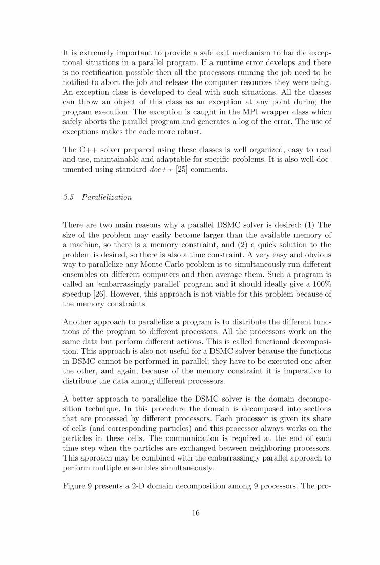
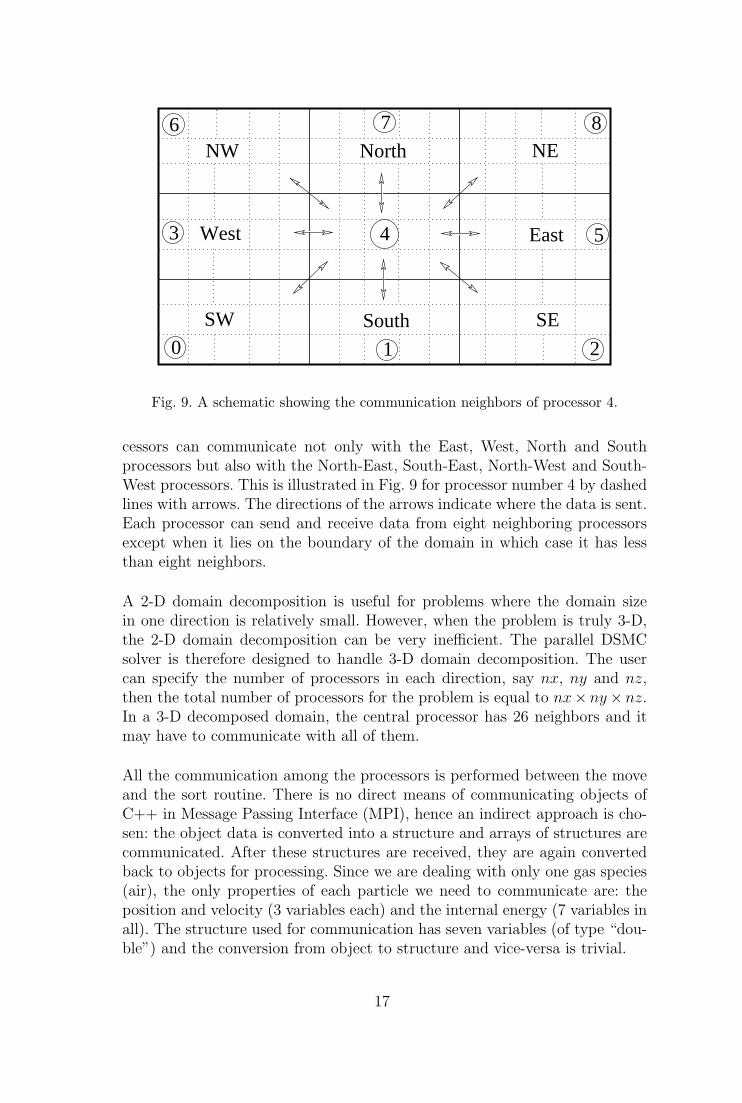
Fig. 9. A schematic showing the communication neighbors of processor 4.

cessors can communicate not only with the East, West, North and Southprocessors but also with the North-East, South-East, North-West and South-West processors. This is illustrated in Fig. 9 for processor number 4 by dashedlines with arrows. The directions of the arrows indicate where the data is sent.Each processor can send and receive data from eight neighboring processorsexcept when it lies on the boundary of the domain in which case it has lessthan eight neighbors.

A 2-D domain decomposition is useful for problems where the domain sizein one direction is relatively small. However, when the problem is truly 3-D,the 2-D domain decomposition can be very inefficient. The parallel DSMCsolver is therefore designed to handle 3-D domain decomposition. The usercan specify the number of processors in each direction, say nx, ny and nz,then the total number of processors for the problem is equal to nx× ny× nz.In a 3-D decomposed domain, the central processor has 26 neighbors and itmay have to communicate with all of them.

All the communication among the processors is performed between the moveand the sort routine. There is no direct means of communicating objects ofC++ in Message Passing Interface (MPI), hence an indirect approach is cho-sen: the object data is converted into a structure and arrays of structures arecommunicated. After these structures are received, they are again convertedback to objects for processing. Since we are dealing with only one gas species(air), the only properties of each particle we need to communicate are: theposition and velocity (3 variables each) and the internal energy (7 variables inall). The structure used for communication has seven variables (of type “dou-ble”) and the conversion from object to structure and vice-versa is trivial.

17

A few important things to keep in mind when parallelizing a particle methodsolver are: Firstly, the number of particles to be communicated changes eachtime step, so the size of the array that is transferred has to be communicatedto the corresponding processor before the particles are exchanged. Secondly,when all the communication is performed the array of objects of particles hasto be rearranged to get rid of the empty spots left by the outgoing parti-cles. The second point appears to be a minor issue but may yield frustratingsegmentation faults if not done properly.

4 Results

The DSMC solver developed for this study is validated against analytical andexperimental results. The Riemann shocktube problem is analytically solvedfor validation, and experimental results from reference [1] on a planar shockinteraction with a square cavity are compared. The different aspects of thesolver such as the solid and inflow boundary conditions are verified againstanalytical solutions of shock reflection from a solid wall, and normal shockrelations.

4.1 The Riemann Problem

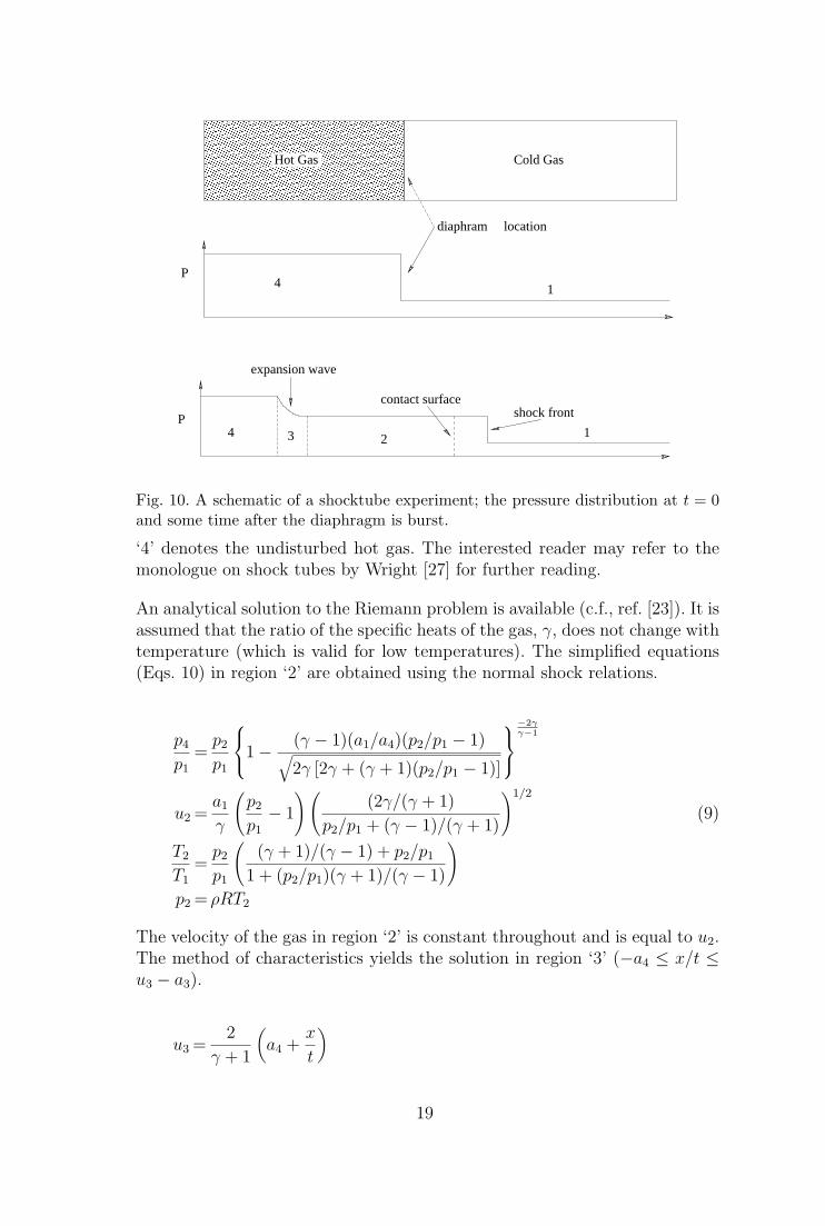
For the Riemann problem, the shocktube is initially divided into two chambersseparated by a diaphragm. One chamber contains a hot gas at high pressureand density and the other contains a cold gas at low pressure and density.The gases in the two chambers may be different but in the present case theyare the same. The diaphragm is then burst instantaneously and the hot gas(driver) is allowed to expand into the cold (driven) section. A shock wave andan expansion wave are formed which travel in opposite directions. The shockwave moves at supersonic speed into the driven section and the expansionwave travels into the driver section. Although the expansion wave travels intothe driver section, the motion of the gas is always in the direction of the shockwave. A schematic of the shocktube problem with the pressure distributionboth before and after the diaphragm is burst is sketched in Fig. 10. Thereare four distinct regions marked ‘1’,‘2’,‘3’ and ‘4’ in Fig. 10. Region ‘1’ isthe cold gas which is undisturbed by the shock wave. Region ‘2’ contains thegas immediately behind the shock traveling at a constant speed. The ‘contactsurface’ across which the density and temperature are discontinuous lies inthis region. If two different gases are used in the driver and the driven sectionthen the contact surface is the interface between the two gases. The regionbetween the head and the tail of the expansion fan is marked ‘3’. In ‘3’ the flowproperties change gradually since the expansion process is isentropic. Region

18

��

��

Hot Gas Cold Gas

14

14 3 2

diaphram location

shock frontcontact surface

expansion wave

P

P

Fig. 10. A schematic of a shocktube experiment; the pressure distribution at t = 0and some time after the diaphragm is burst.

‘4’ denotes the undisturbed hot gas. The interested reader may refer to themonologue on shock tubes by Wright [27] for further reading.

An analytical solution to the Riemann problem is available (c.f., ref. [23]). It isassumed that the ratio of the specific heats of the gas, γ, does not change withtemperature (which is valid for low temperatures). The simplified equations(Eqs. 10) in region ‘2’ are obtained using the normal shock relations.

p4

p1

=p2

p1

1− (γ − 1)(a1/a4)(p2/p1 − 1)√2γ [2γ + (γ + 1)(p2/p1 − 1)]

−2γγ−1

u2 =a1

γ

(p2

p1

− 1

)((2γ/(γ + 1)

p2/p1 + (γ − 1)/(γ + 1)

)1/2

(9)

T2

T1

=p2

p1

((γ + 1)/(γ − 1) + p2/p1

1 + (p2/p1)(γ + 1)/(γ − 1)

)p2 = ρRT2

The velocity of the gas in region ‘2’ is constant throughout and is equal to u2.The method of characteristics yields the solution in region ‘3’ (−a4 ≤ x/t ≤u3 − a3).

u3 =2

γ + 1

(a4 +

x

t

)

19

p3

p4

=[1− γ − 1

2(u3/a4)

]2/(γ−1)

(10)

p3

p4

= (ρ3/ρ4)γ = (T3/T4)

γ/γ−1

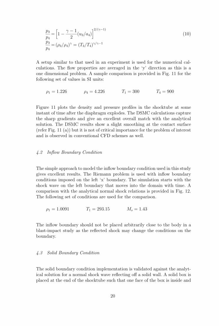
A setup similar to that used in an experiment is used for the numerical cal-culations. The flow properties are averaged in the ‘y’ direction as this is aone dimensional problem. A sample comparison is provided in Fig. 11 for thefollowing set of values in SI units:

ρ1 = 1.226 ρ4 = 4.226 T1 = 300 T4 = 900

Figure 11 plots the density and pressure profiles in the shocktube at someinstant of time after the diaphragm explodes. The DSMC calculations capturethe sharp gradients and give an excellent overall match with the analyticalsolution. The DSMC results show a slight smoothing at the contact surface(refer Fig. 11 (a)) but it is not of critical importance for the problem of interestand is observed in conventional CFD schemes as well.

4.2 Inflow Boundary Condition

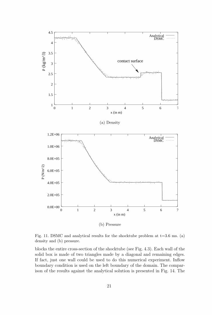
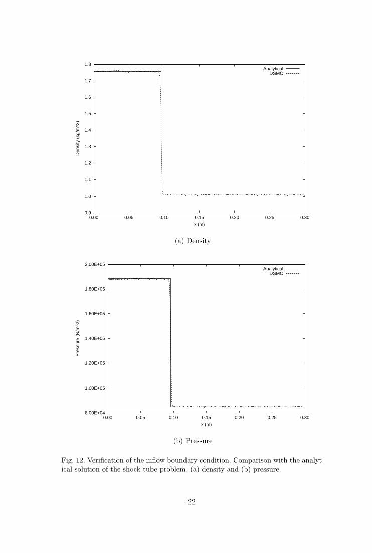
The simple approach to model the inflow boundary condition used in this studygives excellent results. The Riemann problem is used with inflow boundaryconditions imposed on the left ‘x’ boundary. The simulation starts with theshock wave on the left boundary that moves into the domain with time. Acomparison with the analytical normal shock relations is provided in Fig. 12.The following set of conditions are used for the comparison.

ρ1 = 1.0091 T1 = 293.15 Ms = 1.43

The inflow boundary should not be placed arbitrarily close to the body in ablast-impact study as the reflected shock may change the conditions on theboundary.

4.3 Solid Boundary Condition

The solid boundary condition implementation is validated against the analyt-ical solution for a normal shock wave reflecting off a solid wall. A solid box isplaced at the end of the shocktube such that one face of the box is inside and

20

contact surface

(kg/

m^3

)

1

1.5

2

2.5

3

3.5

4

4.5

0 1 2 3 4 5 7

AnalyticalDSMC

6x (in m)

ρ

(a) Density

0.0E+00

2.0E+05

4.0E+05

6.0E+05

8.0E+05

1.0E+06

1.2E+06

0 1 2 3 4 5 6 7x (in m)

AnalyticalDSMC

P (N

/m^2

)

(b) Pressure

Fig. 11. DSMC and analytical results for the shocktube problem at t=3.6 ms. (a)density and (b) pressure.

blocks the entire cross-section of the shocktube (see Fig. 4.3). Each wall of thesolid box is made of two triangles made by a diagonal and remaining edges.If fact, just one wall could be used to do this numerical experiment. Inflowboundary condition is used on the left boundary of the domain. The compar-ison of the results against the analytical solution is presented in Fig. 14. The

21

0.9

1.0

1.1

1.2

1.3

1.4

1.5

1.6

1.7

1.8

0.00 0.05 0.10 0.15 0.20 0.25 0.30

Den

sity

(kg

/m^3

)

x (m)

AnalyticalDSMC

(a) Density

8.00E+04

1.00E+05

1.20E+05

1.40E+05

1.60E+05

1.80E+05

2.00E+05

0.00 0.05 0.10 0.15 0.20 0.25 0.30

Pre

ssur

e (N

/m^2

)

x (m)

AnalyticalDSMC

(b) Pressure

Fig. 12. Verification of the inflow boundary condition. Comparison with the analyt-ical solution of the shock-tube problem. (a) density and (b) pressure.

22

��

��

Hot gas Cold gas

Shock Tube with a solid reflecting wall

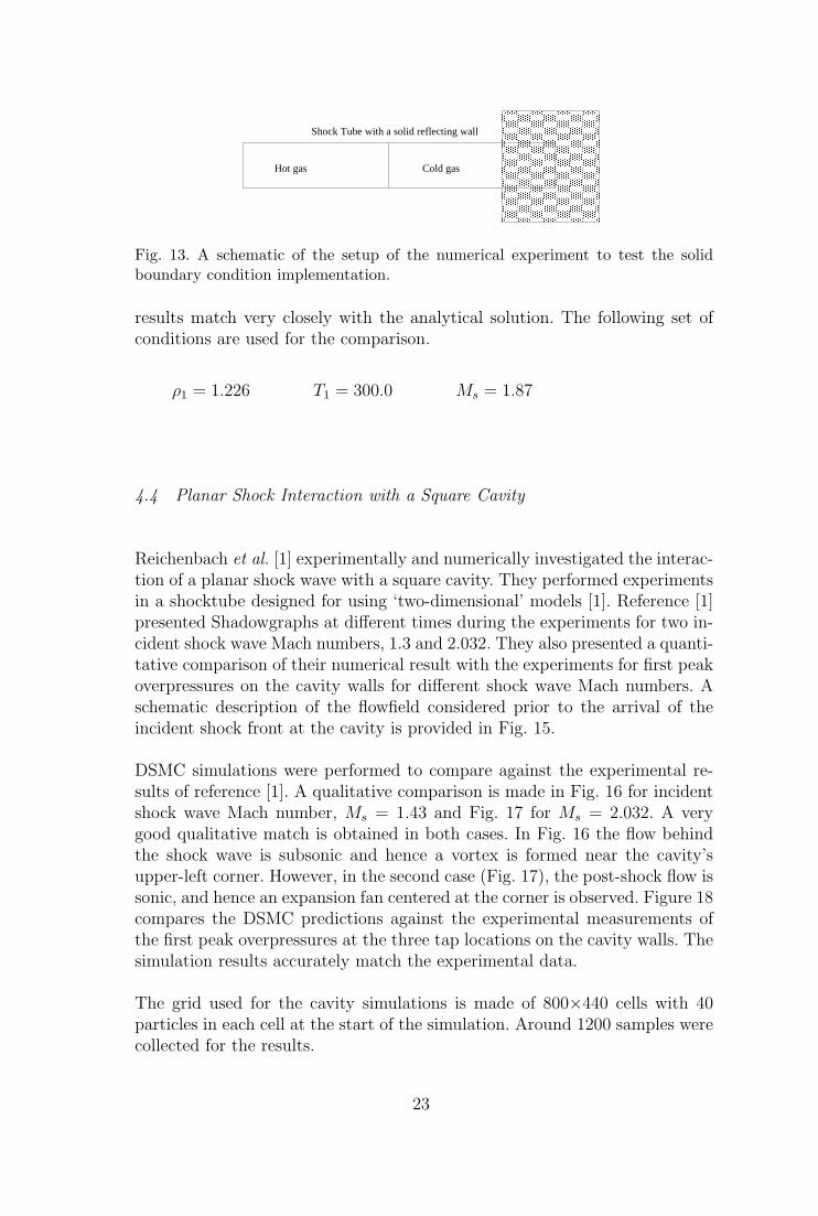
Fig. 13. A schematic of the setup of the numerical experiment to test the solidboundary condition implementation.

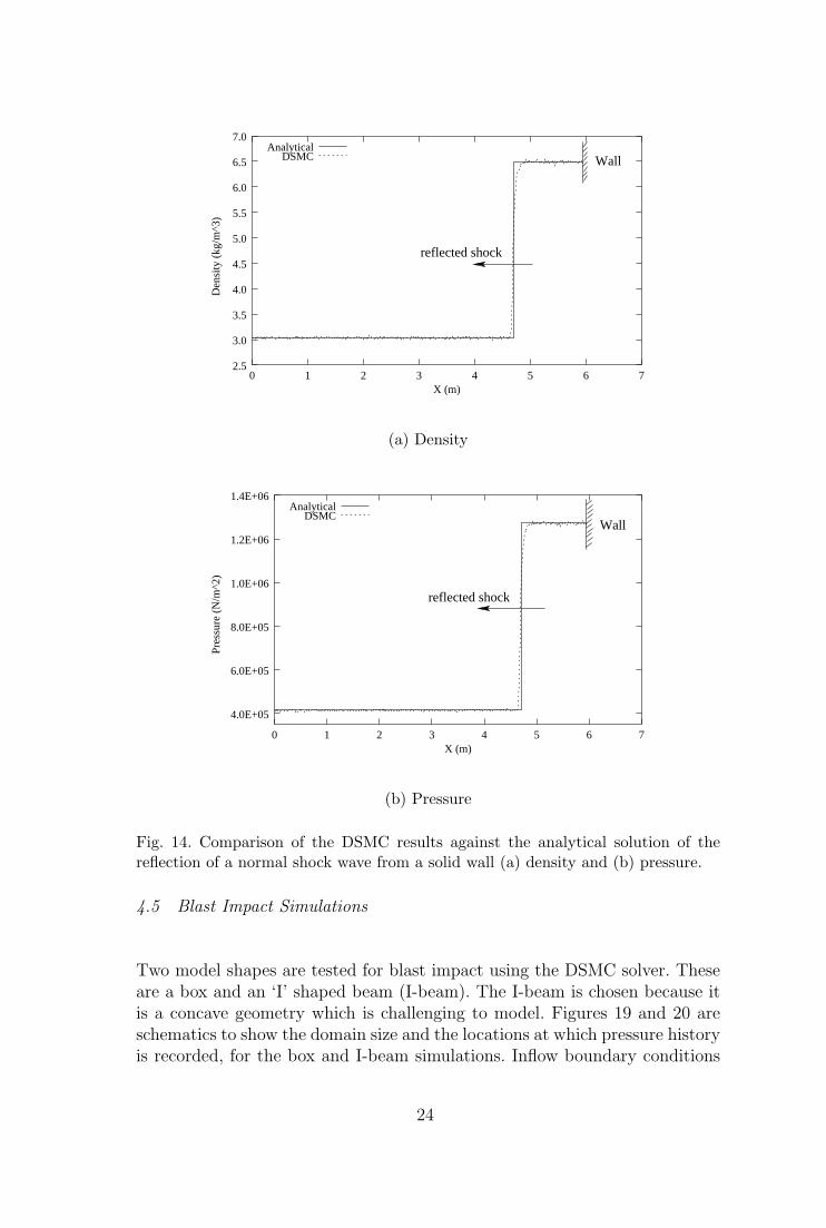
results match very closely with the analytical solution. The following set ofconditions are used for the comparison.

ρ1 = 1.226 T1 = 300.0 Ms = 1.87

4.4 Planar Shock Interaction with a Square Cavity

Reichenbach et al. [1] experimentally and numerically investigated the interac-tion of a planar shock wave with a square cavity. They performed experimentsin a shocktube designed for using ‘two-dimensional’ models [1]. Reference [1]presented Shadowgraphs at different times during the experiments for two in-cident shock wave Mach numbers, 1.3 and 2.032. They also presented a quanti-tative comparison of their numerical result with the experiments for first peakoverpressures on the cavity walls for different shock wave Mach numbers. Aschematic description of the flowfield considered prior to the arrival of theincident shock front at the cavity is provided in Fig. 15.

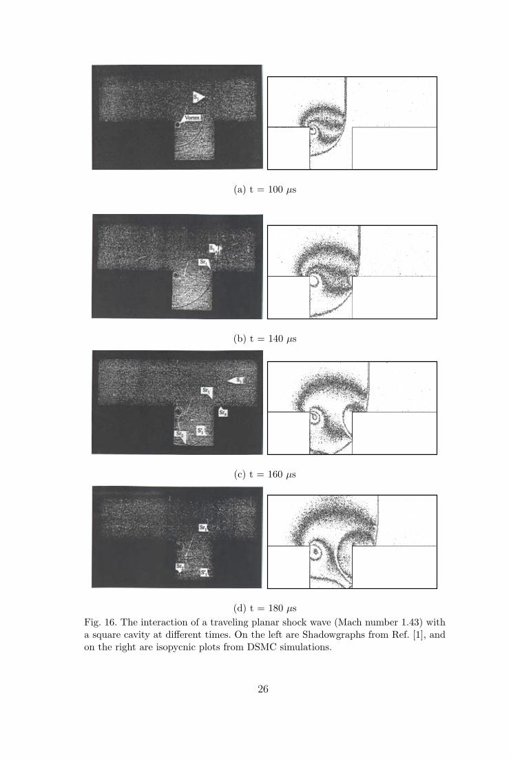
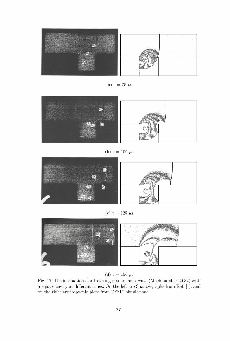
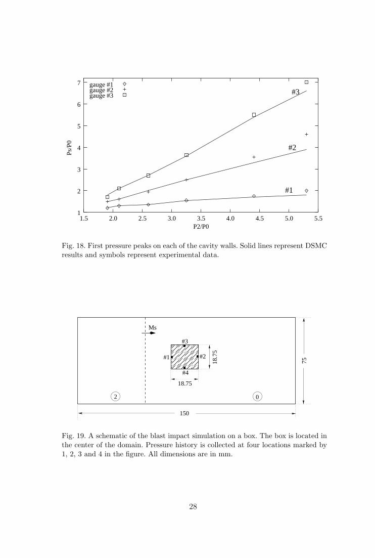
DSMC simulations were performed to compare against the experimental re-sults of reference [1]. A qualitative comparison is made in Fig. 16 for incidentshock wave Mach number, Ms = 1.43 and Fig. 17 for Ms = 2.032. A verygood qualitative match is obtained in both cases. In Fig. 16 the flow behindthe shock wave is subsonic and hence a vortex is formed near the cavity’supper-left corner. However, in the second case (Fig. 17), the post-shock flow issonic, and hence an expansion fan centered at the corner is observed. Figure 18compares the DSMC predictions against the experimental measurements ofthe first peak overpressures at the three tap locations on the cavity walls. Thesimulation results accurately match the experimental data.

The grid used for the cavity simulations is made of 800×440 cells with 40particles in each cell at the start of the simulation. Around 1200 samples werecollected for the results.

23

Wall

reflected shock

2.5

3.0

3.5

4.0

4.5

5.0

5.5

6.0

6.5

7.0

0 1 2 3 4 5 6 7X (m)

AnalyticalDSMC

Den

sity

(kg

/m^3

)

(a) Density

Wall

reflected shock

4.0E+05

6.0E+05

8.0E+05

1.0E+06

1.2E+06

1.4E+06

0 1 2 3 4 5 6 7

Pres

sure

(N

/m^2

)

X (m)

AnalyticalDSMC

(b) Pressure

Fig. 14. Comparison of the DSMC results against the analytical solution of thereflection of a normal shock wave from a solid wall (a) density and (b) pressure.

4.5 Blast Impact Simulations

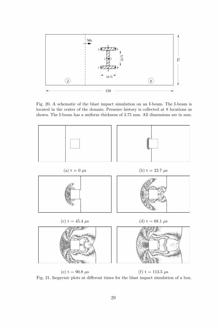
Two model shapes are tested for blast impact using the DSMC solver. Theseare a box and an ‘I’ shaped beam (I-beam). The I-beam is chosen because itis a concave geometry which is challenging to model. Figures 19 and 20 areschematics to show the domain size and the locations at which pressure historyis recorded, for the box and I-beam simulations. Inflow boundary conditions

24

��

��

��

��

50

110

2525

#1 #3

#2

02 Ms

50 50 100

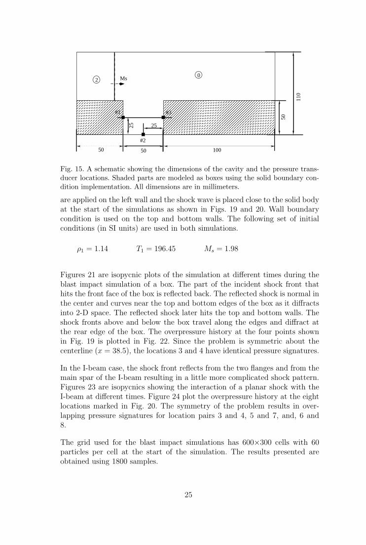
Fig. 15. A schematic showing the dimensions of the cavity and the pressure trans-ducer locations. Shaded parts are modeled as boxes using the solid boundary con-dition implementation. All dimensions are in millimeters.

are applied on the left wall and the shock wave is placed close to the solid bodyat the start of the simulations as shown in Figs. 19 and 20. Wall boundarycondition is used on the top and bottom walls. The following set of initialconditions (in SI units) are used in both simulations.

ρ1 = 1.14 T1 = 196.45 Ms = 1.98

Figures 21 are isopycnic plots of the simulation at different times during theblast impact simulation of a box. The part of the incident shock front thathits the front face of the box is reflected back. The reflected shock is normal inthe center and curves near the top and bottom edges of the box as it diffractsinto 2-D space. The reflected shock later hits the top and bottom walls. Theshock fronts above and below the box travel along the edges and diffract atthe rear edge of the box. The overpressure history at the four points shownin Fig. 19 is plotted in Fig. 22. Since the problem is symmetric about thecenterline (x = 38.5), the locations 3 and 4 have identical pressure signatures.

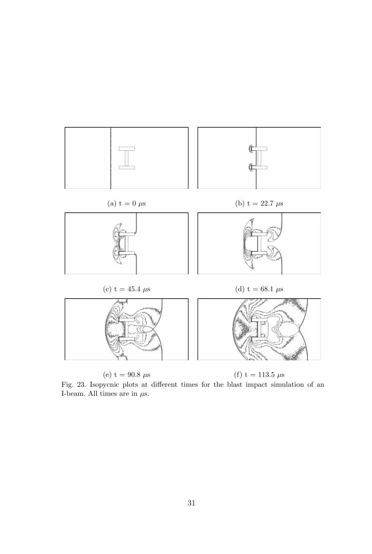
In the I-beam case, the shock front reflects from the two flanges and from themain spar of the I-beam resulting in a little more complicated shock pattern.Figures 23 are isopycnics showing the interaction of a planar shock with theI-beam at different times. Figure 24 plot the overpressure history at the eightlocations marked in Fig. 20. The symmetry of the problem results in over-lapping pressure signatures for location pairs 3 and 4, 5 and 7, and, 6 and8.

The grid used for the blast impact simulations has 600×300 cells with 60particles per cell at the start of the simulation. The results presented areobtained using 1800 samples.

25

(a) t = 100 µs

(b) t = 140 µs

(c) t = 160 µs

(d) t = 180 µsFig. 16. The interaction of a traveling planar shock wave (Mach number 1.43) witha square cavity at different times. On the left are Shadowgraphs from Ref. [1], andon the right are isopycnic plots from DSMC simulations.

26

(a) t = 75 µs

(b) t = 100 µs

(c) t = 125 µs

(d) t = 150 µsFig. 17. The interaction of a traveling planar shock wave (Mach number 2.032) witha square cavity at different times. On the left are Shadowgraphs from Ref. [1], andon the right are isopycnic plots from DSMC simulations.

27

#1

#2

#3

1

2

3

4

5

6

7

1.5 2.0 2.5 3.0 3.5 4.0 4.5 5.0 5.5

Ps/P

0

gauge #1gauge #2gauge #3

P2/P0

Fig. 18. First pressure peaks on each of the cavity walls. Solid lines represent DSMCresults and symbols represent experimental data.

��

��

Ms

150

75

2

#1

#3

#2

18.75

18.7

5

#4

0

Fig. 19. A schematic of the blast impact simulation on a box. The box is located inthe center of the domain. Pressure history is collected at four locations marked by1, 2, 3 and 4 in the figure. All dimensions are in mm.

28

��

��

��

��

Ms

150

75

2 0

487

53

6

21 18.7

5

18.75

Fig. 20. A schematic of the blast impact simulation on an I-beam. The I-beam islocated in the center of the domain. Pressure history is collected at 8 locations asshown. The I-beam has a uniform thickness of 3.75 mm. All dimensions are in mm.

(a) t = 0 µs (b) t = 22.7 µs

(c) t = 45.4 µs (d) t = 68.1 µs

(e) t = 90.8 µs (f) t = 113.5 µsFig. 21. Isopycnic plots at different times for the blast impact simulation of a box.

29

#1

#3,4

#2

−2

0

2

4

6

8

10

12

14

0 0.02 0.04 0.06 0.08 0.1 0.12 0.14 0.16 0.18

Ove

rpre

ssur

e (b

ar)

time(ms)

Fig. 22. Overpressure history at the four locations marked in Fig. 19. Data collectedat every 0.15 µs.

30

(a) t = 0 µs (b) t = 22.7 µs

(c) t = 45.4 µs (d) t = 68.1 µs

(e) t = 90.8 µs (f) t = 113.5 µsFig. 23. Isopycnic plots at different times for the blast impact simulation of anI-beam. All times are in µs.

31

#1

#5,7

#3,4

#6,8

#2

Ove

rpre

ssur

e (b

ar)

−2

0

2

4

6

8

10

12

0 0.02 0.04 0.06 0.08 0.1 0.12 0.14 0.16 0.18time(ms)

Fig. 24. Overpressure history at the eight locations marked in Fig. 20. Data collectedat every 0.15 µs.

4.6 Parallel Performance

The Riemann shocktube, ‘shock interactioni with a cavity’ and the ‘blastimpact on a box’ problems were solved for sample sizes to measure the parallelperformance of the solver. The performance measurements are conducted ontwo Beowulf clusters, COCOA2 and COCOA3. COCOA2 is a 20 node dual800 MHz Pentium III processor cluster with two 100 Mbit Network InterfaceCards (NICs) per node bonded together for interprocessor communication.COCOA3 is a 60 node dual 2.4GHz Xeon processor cluster with one 1 Gbit NICper node. Both the clusters run open-source Redhat linux operating system.The solver was compiled using the open-source GNU compiler, g++ with theoptimization flag -O.

The time taken to perform the key functions in the solver are tabulated inTable 1. The size of the problem is deliberately reduced to allow solution bya single processor. The performance may differ if the domain is decomposedin a different fashion. It is optimized for maximum load balancing for thecases presented here. Figure 25 plots the speedup and the parallel efficienciesobtained for the three problems in Table 1. Appreciable speedup is obtainedeven with a small problem size. Better performance is expected for largerproblem sizes.

32

Table 1Listing of the three sample problems solved on COCOA3 for performance testing.

Case Timing(s)

Procs Move Collide Sample Comm. Total

Riemann 1 999.17 6923.57 30.16 0.00 11278.3Shocktube 2 612.58 3404.70 17.32 34.23 6213.3Cells: 600*100*1 4 327.00 1675.02 8.88 31.83 3201.3Part: 3 mill. 8 182.96 896.70 4.63 99.82 1760.2

16 85.30 422.84 2.33 158.05 936.7

Shock Interaction 1 1780.77 4442.40 21.09 0.00 8640.9With a Cavity 2 1057.07 2543.21 12.69 8.32 5137.4Cells: 400*220*1 4 279.11 828.78 3.19 1968.94 3470.2Part: 4.4 mill. 8 43.97 75.95 0.45 2062.24 2233.9

16 0.31 0.40 0.03 985.49 990.8

Blast Impact 1 1243.73 6251.45 20.48 0.00 9781.5With a Box 2 701.84 3117.28 11.62 29.25 5204.4Cells: 400*220*1 4 318.60 1499.78 5.58 133.32 2592.4Part: 4.4 mill. 8 159.68 774.33 2.79 120.22 1375.1

16 76.99 381.08 1.27 60.05 673.7

5 Conclusions

The problem of blast wave interaction with structures is studied using theDirect Simulation Monte Carlo approach. A new approach to model the solidboundary condition for complex geometries is described and implemented withsuccess. The Object Oriented approach used for the development of the solveris described. The code is made parallel using the domain decomposition tech-nique to solve large, complex problems. Different aspects of the solver areindividually validated against analytical results for benchmark problems. Re-flection of a normal shock from a wall is used to validate the solid boundarycondition and normal shock relations are used to validate the inflow boundarycondition. The Riemann shocktube problem and experimental results from anexperiment on planar shock interaction with a cavity (ref. [1]) are used tovalidate the solver. Both qualitative and quantitative comparisons are madefor the shock-cavity interaction problem. The numerical results are found tobe in excellent agreement with the experiments.

The problem of blast impact is studied on two model shapes: a box and anI-beam. Pressure signatures at a few locations are plotted to provide a quan-titative measure of the loading. Isopycnic plots showing the flow structure are

33

0

2

4

6

8

10

12

14

16

0 2 4 6 8 10 12 14 16

Alg

orith

mic

Spe

edup

Number of Processors of COCOA2

IdealRiemann

CavityBox

0

2

4

6

8

10

12

14

16

0 2 4 6 8 10 12 14 16

Alg

orith

mic

Spe

edup


IdealRiemann

CavityBox

(a) Algorithmic Speedup

0

20

40

60

80

100

0 2 4 6 8 10 12 14 16

Par

alle

l Effi

cien

cy


IdealRiemann

CavityBox

0

20

40

60

80

100

0 2 4 6 8 10 12 14 16

Par

alle

l Effi

cien

cy


IdealRiemann

CavityBox

(b) Parallel Efficiency

Fig. 25. The performance of the parallel program for three test cases tabulated inTable 1 on COCOA2 (left) and COCOA3 (right).

presented at different times. Lastly, the parallel performance of the solver isestimated on two Beowulf clusters for three problems.

References

[1] O. Igra, J. Falcovitz, H. Reichenbach, W. Heilig, Experimental and NumericalStudy of the Interaction between a Planar Shock Wave and a Square Cavity,Journal of Fluid Mechanics 313 (1996) 105–130.

[2] G. A. Bird, Molecular Gas Dynamics, Clarendon Press, Clarendon, Oxford,1976.

[3] E. P. Muntz, Rarefied Gas Dynamics, Annual Review of Fluid Mechanics 21(1989) 387–417.

34

[4] E. Salomons, M. Mareschal, Usefulness of the Burnett Description of StrongShock Waves, Physical Review Letters 69 (2) (1992) 269–272.

[5] G. A. Bird, Monte Carlo Simulation of Gas Flows, Annual Review of FluidMechanics 10 (1978) 11–31.

[6] G. A. Bird, Molecular Gas Dynamics and the Direct Simulation of Gas Flows,2nd Edition, Oxford Science Publications, Clarendon, Oxford, 1994.

[7] D. I. Pullin, J. Davis, J. K. Harvey, Monte Carlo Calculations of the RarefiedTransition Flow Past a Bluff Faced Cylinder, in: 10th International Symposiumon Rarefied Gas Dynamics, Aspen, Colorado, 1976.

[8] E. S. Oran, C. K. Oh, B. Z. Cybyk, Direct Simulation Monte Carlo : RecentAdvances and Application, Annual Review of Fluid Mechanics 30 (1998) 403–441.

[9] G. A. Bird, Direct Simulation of the Boltzmann Equation, Physics of Fluids 13.

[10] L. N. Long, Navier Stokes and Monte Carlo Results for Hypersonic Flows, AIAAJournal 29 (2).

[11] J. B. Anderson, L. N. Long, Direct Monte Carlo Simulation of ChemicalReaction Systems: Prediction of Ultrafast Detonations, The Journal of ChemicalPhysics 118 (7) (2003) 3102–3110.

[12] L. N. Long, J. B. Anderson, The Simulation of Detonations using a Monte CarloMethod, in: Rarefied Gas Dynamics Conference, Sydney, Australia, 2000.

[13] J. B. Anderson, L. N. Long, Direct simulation of pathological detonations, in:18th International Symposium on Rarefied Gas Dynamics, Vancouver, Canada,2002.

[14] S. M. Dunn, J. B. Anderson, Direct Monte Carlo Simulation of ChemicalReaction Systems: Internal Energy Transfer and an Energy-DependentUnimolecular Reaction, The Journal of Chemical Physics 99 (9) (1993) 6607–6612.

[15] S. M. Dunn, J. B. Anderson, Direct Monte Carlo Simulation of ChemicalReaction Systems: Dissociation and Recombination, The Journal of ChemicalPhysics 102 (7) (1995) 2812–2815.

[16] W. Wagner, A Convergence Proof for Bird’s Direct Simulation Monte CarloMethod for the Boltzmann Equation, Journal of Statistical Mechanics 66 (3/4).

[17] D. I. Pullin, Direct Simulation Methods for Ideal-Gas Flow, Journal ofComputational Physics 34 (1980) 231–244.

[18] C. L. Merkle, H. William Behrens, Robert D. Hughes, Application of theMonte-Carlo Simulation Procedure in the Near Continuum Regime, in: TwelfthSymposium on Rarefied Gas Dynamics, 1980.

35

[19] A. Sharma, L. N. Long, T. Krauthammer, Using the Direct Simulation MonteCarlo Approach for the Blast-Impact Problem, in: The 17th InternationalSymposium on Military Aspects of Blast Simulations, Las Vegas, Nevada, 2002.

[20] A. L. Danforth, L. N. Long, Acoustic Propagation using the Direct SimulationMonte Carlo Method, The Journal of the Acoustical Society of America 114 (4)(2003) 2356–2357.

[21] N. G. Hadjiconstantinou, A. L. Garcia, Molecular Simulations of Sound WavePropagation in Simple Gases, Physics of Fluids 13 (2001) 1040–1046.

[22] I. E. Sutherland, R. F. Sproull, R. Shumacker, A Charaterizarion of Ten HiddenSurface Algorithms, ACM Computing Surveys 6 (1) (1974) 1–55.

[23] J. D. Anderson Jr., Modern Compressible Flow with Historical Perspective, 2ndEdition, McGraw Hill Professional Publishing, 1989.

[24] Claus Borgnakke, Poul S. Larsen, Statistical Collision Model for Monte CarloSimulation of Polyatomic Gas Mixture, Journal of Computational Physics 18(1975) 405–420.

[25] Doc++ homepage:, http://docpp.sourceforge.net.

[26] L. N. Long, K. S. Brentner, Self-Scheduling Parallel Methods for Multiple SerialCodes with Applications to wopwop, in: 38th Aerospace Sciences and MeetingExhibit, Paper 0346, Reno, Nevada, 2000.

[27] J. K. Wright, Shock Tubes, John Wiley & Sons INC, 1961.

36

http://docpp.sourceforge.net

numerical simulation of the blast impact problem …

Documents