numerical simulation of supersonic and turbulent ...mkamel/publications/mkamel-ijesms-2015-7_… ·...

Numerical Simulation of Supersonic & Turbulent Combustion with Transverse Sonic Fuel Injection 1

Numerical Simulation of Supersonic andTurbulent Combustion with TransverseSonic Fuel Injection

Mohammed Kamel1, Farouk Owis2,Moumen Idres3, Aly Hashem4

Aerospace Engineering Department - Faculty of EngineeringCairo University, Giza, [email protected]@eng.cu.edu.eg (Corresponding Author)[email protected]@eng.cu.edu.eg

Abstract Complicated interacting flow features such as shock-wave,boundary-layer and shock induced combustion are simulated numerically inthe current study to investigate the e↵ect of the transverse sonic fuel injectionon the air-fuel mixing and flame stabilisation. The flow is modelled using theReynolds-averaged Navier-stocks (RANS) equations, where chemical kineticsmodel is employed to compute the finite rates of chemical reactions. Turbulenceis modelled using the Baldwin-Lomax algebraic model. Finite-volume schemeis applied where the convective fluxes are discretised by second order accurateRoe?s scheme using MUSCL approach. Second order accurate Runge-Kuttamethod is used for the time-integration. Turbulent and chemically-reacting su-personic flow of hydrogen-air mixture over a ramp is simulated and the resultsshow good agreement with the experimental data and the published numericalsimulations In addition, air-hydrogen flow is studied in a single strut scram-jet engine, where mixing and flame holding processes are carried out using fueltransverse sonic injection.

Keywords: Scramjet Engines; Computational Fluid Dynamics; Chemically-Reacting Flows; Reynolds-Averaged Navier-Stocks; Turbulent Flows; Super-sonic Combustion

Biographical Notes:� Mohammed Kamel is a Lecturer Assistant in Cairo University, where hereceived his MSc in 2009. Currently, he is a PhD student in the University ofNotre Dame, USA. His areas of interests are computational fluid dynamics, re-acting flows simulation, and turbulence modelling.� Farouk Owis is an Associate Professor in Cairo University, where he re-ceived his MSc in 1993. In 1999, he received his PhD from Old Dominion Uni-versity, USA. His fields of interest cover computational fluid dynamics, turbo-machinery, jet engine propulsion, and renewable energy.� Moumen Idres received his BSc and MSc in Cairo University in 1992 and1995, respectively. In 1999, he received his PhD from Old Dominion Univer-sity, USA. He is on leave from Cairo University. Currently, he is an AssistantProfessor in the International Islamic University Malaysia. He has researchpublications in aerospace propulsion, vehicle power systems, combustion andcomputational fluid mechanics.� Aly Hashem has been a Professor of Aircraft Propulsion, Cairo Universitysince 2005. He received his MSc and PhD from Cranfield Institute of Technol-ogy, School of Mechanical Engineering, UK in 1974 and 1977, respectively. Hisareas of interests concern turbo-machinery, jet engine propulsion, renewableenergy and combustion.

1 Introduction

Flows with chemical reactions are of interest acrossa wide range of engineering applications includingsupersonic combustion, space vehicle reentry, androcket plume problems. A great amount of e↵orthas been focused in the areas of algorithm devel-opment and thermo-chemical modeling for theseflows. The modeling of chemically reacting turbu-lent flows at supersonic speeds has been attemptedby many investigators (2; 3). However, the physicaland mathematical complexities of this problem haveprevented the development of satisfactory modelsfor the turbulence and combustion mechanisms andtheir influence on each other in a compressible flow-field. A relatively recent review by Cinnella andGrossman (4) provides details on numerical meth-ods for chemically reacting flows. There is still acontinuing e↵ort to better understand these com-plex flow phenomenon.

The objective of the current study is to develop anaccurate numerical tool for the simulation of turbu-lent and supersonic chemically-reacting flows. Thecode is used to investigate numerically the e↵ectof transverse fuel injection on the air-fuel mix-ing and flame holding. This work is motivated bythe need to simulate flowfields present in a typicalsupersonic combustion ramjet (SCRAMJET) en-gine where flame-holding in the supersonic flowfieldis attained by providing the necessary activationenergy for combustion initiation in very small frac-tion of time. Shock-induced combustion, or plasmatorches are the most feasible flame-holding candi-dates. However, transverse sonic fuel injection intosupersonic air inlet flow is one of the most e�cienttechniques suggested to enhance both air-fuel mix-ing and flame holding, as introduced by Drummond(1). Transverse sonic injection of the gaseous fuelinto the air supersonic stream leads to rapid air-fuelmixing. Transverse injection configuration can bemanipulated to obtain optimum heat release for awide range of flight Mach numbers.

The developed code is utilized to simulate thechemically reacting turbulent flows inside scramjetengine. The code is validated by considering sev-eral test cases. The code is then used to resolvethe complicated flowfield accompanying the sonictransverse injection of Helium into supersonic airflow. The results are compared with the previousresults of Kraemer and Rogers experiment reportedby Durmmond et al. (26). In addition, the turbu-lent chemically non-reacting flows inside scramjet

engines are also simulated in the current study.This non-reacting case is simulated for turbulentflow inside single strut scramjet engine as intro-duced by Drummond and Weidner (26).

Di↵erent features of turbulent flows, which aregenerally modeled using unsteady Navier-Stokesequations, can be resolved by time-averaging ap-proaches such as Reynolds averaged Navier-Stocksequations (RANS). It can also be resolved usingspace-averaging approaches such as Large EddySimulation (LES). Large Eddy Simulation solvesthe filtered spatial-averaged large-scale componentsof turbulence (on the order of 90% of transportcomponents), where the small scales are modeled.On the other hand, Direct Numerical Simulation(DNS) considers all flow features with all relevantlength scales to be resolved from the smallest eddiesto scales on the order of the physical dimensionsof the problem domain. Despite the shortcomingsassociated with the statistical representation oftime-averaging RANS closures, RANS equationsstill show e�ciency in most test cases. As, it re-quires much less computational e↵ort than thatrequired by LES or DNS approaches (5; 6). Themathematical model used in the current simulationis the unsteady Reynolds-Averaged Navier-Stocksequations (RANS). Finite-volume discretization isemployed for the numerical integration of the gov-erning equations. The second-order Roe’s schemeis used for spatial discretization. Total variation di-minishing are achieved by using minmode limiter.A two-step second order accurate Runge-Kutta isused for the time integration. Point-implicit schemeis applied for the chemical source term to reducethe sti↵ness of the system.

Turbulence modeling based on Boussinseq’s as-sumption, are divided into numerous categoriesaccording to the number of the additional partialdi↵erential equations. There are the field two-equations turbulence models such as (k-✏) model(7; 8), and (k-!) model (9). In addition, thereare the One-Equation Turbulence Models such asBaldwin-Barth model (10). Zero-Equation modelsrequire an algebraic equation solution to obtainthe turbulent flow properties such as Cebeci-Smithmodel (11) and Baldwin-Lomax model (12). Alge-braic models are widely used due to its simplicityand robustness although they give inaccurate es-timations in strong flow separations (13). In thecurrent study, zero- equation of Baldwin-Lomax areused to calculate the turbulent eddy viscosity.

2


In supersonic combustion, the order of magnitudeof characteristic time of the chemical reactions ismuch less than that of flow residence time. There-fore, sti↵ness of the source terms arises from thegreat gap between the time scales of the coupledgoverning equations. Full implicit treatment ofthe governing equations for two-dimensional flowsleads to the solution of simultaneous equationsin pent-block diagonal matrix form. Di↵erent fac-torization methods are testified in fully implicitsolver (14). It is found that the iterative methodof Lower-Upper Symmetric Gauss-Siedel (LUSGS)method (15) shows the fastest convergence rates forimplicit solvers of 2D domains. In order to reducethe computational e↵orts of inverting the flow Ja-cobians, the convective and viscous flow fluxes aretreated explicitly, where only the chemical sourceterm is solved implicitly. This method is well-knownas Chemistry-Implicit or Point-Implicit. It is in-troduced by Curtiss and Hirschfelder (16). In thiscase, a mono-block diagonal matrix will be solved.Thus, the computational e↵ort is greatly reduced.

Flux-vector and flux-di↵erence splitting schemesare numerically applied by Grossman et al (17) tosimulate chemically and thermally non-equilibriumone-dimensional flows. More extensions for multi-dimensional problems are presented by Walters etal. (18), where two reacting mechanisms of H2-airare studied. Bussing and Murman (20; 21) used afinite volume point-implicit method with multi-gridaccelerator. Shuen and Yoon (22) employed fullyimplicit finite-volume with lower-upper symmet-ric successive over-relaxation scheme (LUSSOR).Their model is coupled with chemical kineticsmodel of 8-species and 14-reactions model (23). Ek-lund et al. (24) studied relative merits of Adamand Runge-Kutta schemes. Partial implicit methodand the global two-step chemistry model (19) wasused successfully by Drummond, et al. (25) to cal-culate premixed Hydrogen-air reacting flow using aspectral method. Drummond and Weidner solvedtransverse sonic injection of hydrogen into super-sonic air flow in a single strut scramjet engineusing the finite di↵erence scheme of MacCormakwith complete chemical reaction model (26). Chit-somboon and Tiwari (27; 28) used also a finitedi↵erence method for similar problems.

2 Mathematical Modeling

2.1 Governing Equations

The governing Equations are the Reynolds time av-eraging Navier Stocks equations. The conservativenon-dimensional form of RANS equations for two-dimensional flow is written as follows,

@Q

@t+@E

@x+@F

@y+ ↵H =

=@E

v

@x+@F

v

@y+ ↵H

v

+ S (1)

Where ↵ is a logical switch between planar and 2Daxisymmetric two-dimensional flows. S representsthe chemical source term.

Q = [⇢, ⇢u, ⇢v, ⇢Et

, ⇢Ym

]T (2)

E =

2

66664

⇢u⇢u2 + P⇢uv⇢H

t

u⇢Y

m

u

3

77775F =

2

66664

⇢v⇢uv

⇢v2 + P⇢H

t

v⇢Y

m

v

3

77775(3)

Ev

=

2

66664

0⌧xx

p

⌧xy

⌧xx

p

u+ ⌧xy

v � qx

�dmx

3

77775

Fv

=

2

66664

0⌧xy

⌧yy

p

⌧xy

u+ ⌧yy

p

v � qy

�dmy

3

77775(4)

↵ =

⇢0, Planar 2DFlow1, Axisymmertic 2DFlow

(5)

H =1

y

2

66664

⇢v⇢uv⇢v2

⇢Ht

v⇢Y

m

v

3

77775(6)

Hv

=

2

6666664

0⌧

xy

y

+ @⌧

a

@x

⌧

yy

p

+⌧

a

�⌧

✓✓

y

+ @⌧

a

@y

⌧

xy

u+[⌧yy

p

+⌧

a

]v�q

y

y

+⇣

@(⌧a

u)@x

+ @(⌧a

v)@y

⌘

�d

my

y

3

7777775(7)

S = [0, 0, 0, 0, !̇m

]T (8)

4 M. Kamel et al.

The governing equations are non-dimensionalizedwith respect to reference values of the characteristicdimensions of the problem which are denoted L

ref

, ⇢ref

, Vref

, Tref

.

2.2 Thermodynamic Model

The mixture enthalpy and internal energy are cal-culated by summation of the species contributions.

h =n

sX

m=1

Ym

hm

e =n

sX

m=1

Ym

em

(9)

The non-dimensional enthalpy for individual speciesis determined by:

hm

=1

V 2ref

2

4ho

f

m

+

T

⇤Z

T

o

cp

m

dT ⇤

3

5 (10)

where: T ⇤ = T.Tref

, and ho

f

m

is the species heat offormation. We assume that specific heat coe�cientfor each species (c

p

m

) is a polynomial function intemperature (T ) as given by Mcbride et al. (31).The total mixture enthalpy and internal energy aredescribed as:

Ht

=

ho

f

mix

+T

⇤R

T

o

cp

mix

d⌧ +(u2+v

2)2

V 2ref

(11)

Et

=

ho

f

mix

+T

⇤R

T

o

(cp

mix

�Rmix

) d⌧ +(u2+v

2)2

V 2ref

(12)

where ho

f

mix

, cp

mix

, andRmix are the mixture’s heatof formation, heat coe�cient at constant tempera-ture, and gas constant:

ho

f

mix

=nsP

m=1Ym

ho

f

m

cp

mix

=nsP

m=1Ym

cp

m

Rmix

=nsP

m=1Ym

Rm

(13)

The equation of state of the gaseous mixture can bewritten as,

P =Tref

V 2ref

⇢Rmix

T (14)

where (hs

) and (es

) are the mixture sensible en-thalpy and sensible internal energy respectively willbe defined as follows,

hs

= h� ho

f

mix

=T

⇤R

T

o

cp

mix

dT ⇤

es

= e� ho

f

mix

=T

⇤R

T

o

(cp

mix

�Rmix

) dT ⇤(15)

It can be shown that:

hs

� es

=P

⇢� R

mix

V 2ref

To

(16)

The reference temperature degree (To

) is set to bethe absolute zero to ensure positive sensible en-thalpy and sensible internal energy and to enhancethe stability of the numerical solution as recom-mended by Anderson (34). Also, the ratio of themixture sensible enthalpy to the mixture internalenergy is considered as the “equivalent” specific ra-tio of the multi-species mixture to simplify the com-plexity of the thermodynamic relations as discussedby Shuen and Yoon (22).

� =hs

es

=

T

⇤Z

T

o

cp

mix

dT ⇤

T

⇤Z

T

o

(cp

mix

�Rmix

) dT ⇤

(17)

So, the relation between the mixture pressure anddensity to the mixture sensible internal energy be-comes,

P

⇢= e

s

(� � 1) (18)

2.3 Turbulent Dynamic Viscosity Modeling

Algebraic Baldwin-Lomax turbulence model is ap-plied to calculate the turbulent eddy coe�cient eddy(µ

T

). A two-layer turbulence model; where the tur-bulent dynamic viscosity coe�cient (µ

T

) is calcu-lated with one of two di↵erent sets of algebraic equa-tions depending on the distance (n) from boundarywalls, or jets centerlines:

µT

=

⇢µT

in

, n ncross

µT

out

, n > ncross

(19)

The turbulent viscosity profile µT

for the two-layermodel is calculated as follow,

µT

= min (µT

in

, µT

out

) . (20)

• Inner Region In the inner region, eddy vis-cosity coe�cient (µ

T

in

) is calculated in termsof the mixing length (l

mix

), and the vorticityvector magnitude (!) as follows,

µT

in

= ⇢l2mix

! (21)

where:

! =

s@u

@y+@v

@x

�2(22)


lmix

= n⇣1� e�n

+/A

+⌘

(23)

The damping factor (e�n

+/A

+

) is eliminatedfor the cases of wakes and jets.

• Outer Region The eddy viscosity of theouter layer (µ

T

out

) is calculated as follows,

µT

out

= ⇢KCcp

Fwake

FKlep

(24)

The normal distance (n) and velocity (V ) are nor-malized to (n+) and (u+) using the friction velocity(u

⌧

) and flow variables at the wall surface.

u⌧

=

r⌧w

⇢w

, n+ =u⌧

⇢w

n

µL

w

, u+ =V

u⌧

(25)

The other terms in equation (24) are written in thefollowing form:

Fwake

= min

✓nmax

Fmax

, Cwk

nmax

u2di↵

Fmax

◆(26)

FKleb

=

"1 + 5.5

✓nC

Kleb

nmax

◆6#�1

(27)

where (udi↵) is the di↵erence between the maximumand minimum velocity magnitudes in the bound-ary layer. So in the wall-bounded domains the mini-mum velocity equals zero and udi↵ = V

max

. Besides,(F

max

) is the max value of the intermediate func-tion F (n) along a certain line normal to the wall ornormal to the centerline of the jet. This function iswritten as follows,

F (n) =1

lmix

! (28)

Fmax

= maxn

[F (n)] (29)

nmax

= n|F

max

(30)

nmax

is the normal distance (n) at which the func-tion (F ) reaches its maximum value. This turbu-lence approach consists of six closure constant listedbelow according to Baldwin and Lomax (12):

A+ = 26 Ccp

= 1.6CKleb

= 0.3C

wk

= 0.25 = 0.4 K = 0.0168(31)

In spite of the excellent performance of the Bald-win and Lomax method in solving attached flows,it predicts incorrectly the separation point locationfor strong pressure gradients. Degani and Schi↵ (13)added some modifications to the previous modelto eliminate the reasons leading to the model de-ficiency when used in separated flows. They found

that there are dramatic di↵erences in the behaviorof the intermediate function F (n) in the attachedand separated flows, which have considerable e↵ectson the calculations. It is found that there is one lo-cal maximum point in the function F (n), where theglobal maximum of the function (F

max

) can be es-timated. However, in separated flows, there will bemultiple local maxima. By implementing equation(29)to get (F

max

), the global maximum will be se-lected, which is not considered the right choice. Thelocal maxima far away from the wall or jets repre-sents recirculating zone of high vorticity magnitude.The right choice is to select the nearest local max-imum from the wall or jet centerline to be used inthe turbulence model calculations with the physicalcorrect values of F

max

and nmax

.

2.4 Mass and Heat Fluxes Modeling

The di↵usive mass fluxes dmx

and dmy

of the mth

species in the x and y directions are written as fol-lows,

dmx

=�1

Reref

Scref

✓⇢D

L

+µT

ScT

Scref

◆@Y

m

@x

dmy

=�1

Reref

Scref

✓⇢D

L

+µT

ScT

Scref

◆@Y

m

@y(32)

DL

is the laminar mass di↵usivity coe�cient of mth

species into the mixture which is assumed constantfor all species.. In addition, Sc

ref

is the problemcharacteristic “Schmidt number”, which is given as:

Scref

=µref

⇢ref

Dref

(33)

On the other hand, the heat fluxes in the x and ydirections are written as follows,

qx

=1

Reref

"�1

(�ref

� 1)M2ref

Prref

kL

@T

@x

� 1

Scref

n

sX

m=1

hm

⇢DL

@Ym

@x� µ

T

PrT

@h

@x

#

qy

=1

Reref

"�1

(�ref

� 1)M2ref

Prref

kL

@T

@y

� 1

Scref

n

sX

m=1

hm

⇢DL

@Ym

@y� µ

T

PrT

@h

@y

#(34)

Mref

and Prref

are the reference values of “Machnumber” and “Prandtl number” respectively. Theturbulent terms of “Schmidt number” (Sc

T

) and“Prandtl number” (Pr

T

) are utilized to model the

6 M. Kamel et al.

mass and heat turbulent fluxes respectively. Bothare set to be 0.9. Modeling of mass and heat lami-nar transport coe�cients (i.e. D

L

and kL

) is basedon assuming constant values of the laminar terms of“Prandtl number”(Pr

L

) and “Lewis number” (Le).Pr

L

is assumed to be 0.72 according to ref. (28),while Le is set to unity. Based on the previous as-sumptions, k

L

and DL

are determined as follows,

kL

=cp

mix

µL

PrL

(35)

DL

=kL

⇢ Le cp

mix

(36)

2.5 Chemistry Modeling

Decoupling between chemistry and turbulence mod-els is adopted in this study. The random fluctua-tions in the magnitudes of temperature and massfractions are not considered in the calculations ofthe species source terms. For chemically reactingnon-equilibrium air-Hydrogen system, the combus-tion process is modeled using a mechanism com-posed of a number of elementary reactions, not onlyone global reaction. Each elementary equation canbe written as following:

⌫0m,r

Xm

kf

⌦kb

⌫00m,r

Xm

(37)

(⌫0) and (⌫00) are the stoichiometric coe�cients ofthe reactants and products respectively of each ele-mentary reaction of index (r), where r = 1, 2, .., n

r

,where (n

r

) is the total number of elementary reac-tions in the mechanism. (k

f

) and (kb

) are the chemi-cal reaction rates in the forward and backward direc-tions respectively. The source term of each speciesof index (“m00) is calculated using the “law of massaction”. It is written in the dimensionless form asfollows,

!̇m

=

L

ref

⇢

ref

V

ref

Mm

n

rPr=1

2

66664

(⌫0m,r

� ⌫00m,r

) ⇤⇤✓kfr

n

sQm=1

⇣⇢Y

m

Mm

⌘⌫

0m,r

+

�kbr

n

sQm=1

⇣⇢Y

m

Mm

⌘⌫

00m,r

◆

3

77775(38)

The forward reaction rate (kf

) is calculated us-ing the Arrhenius’ formula whose coe�cients andthe temperature exponent is determined experimen-tally. It is written for each elementary reaction ofindex (r) as follow,

kfr

= Ar

TNr exp

✓�Eactv,r

R T

◆(39)

Air-Hydrogen combustion system is modeled byusing the two reactions mechanism suggested byRogers and Chinitz (19). This two reactions modelincludes four reacting species (O2, H2O, H2, andOH), besides Nitrogen N2, which is assumed to beinert, because the mixture temperature is not toohigh to initiate the Nitrogen-Oxides formation;

O2 +H2

kf1

⌦kb1

2OH (40)

2OH + H2

kf2

⌦kb2

2H2O (41)

The forward reaction rates for the two reactions arewritten as follows,

kf1 = A1T

�10 exp

✓�4063.6485

RT ⇤

◆

kf2 = A2T

�13 exp

✓�35499.4988

RT ⇤

◆(42)

In equation (42), the units of the universal gas con-stant (R) is [kcal/kmole K]. The pre-exponentialcoe�cients for the elementary reaction are functionof the equivalence ratio (�), as follows,

A1 =h8.917�+ 31.433

�

� 28.95i(10)44

hm

3/kmol

sec

i

A2 =h2 + 1.333

�

� 0.833�i(10)58

hm

3/kmol

sec

i (43)

3 Numerical Treatment

The governing equations can be written in the com-putational domain in the following form:

@Q

@t+@E

@⇠+@F

@⌘+ ↵H =

@Ev

@⇠+@F

v

@⌘+ ↵H

v

+ S,(44)

where:

Q =1

JQ,

E =1

J(⇠

x

E + ⇠y

F ) , F =1

J(⌘

x

E + ⌘y

F ),

Ev

=1

J(⇠

x

Ev

+ ⇠y

Fv

) , Fv

=1

J(⌘

x

Ev

+ ⌘y

Fv

),

H =1

JH, H

v

=1

JH

v

, S =1

JS,

(45)

The finite volume method is used to discretize thegoverning equations at each cell in the computa-tional domain. Starting from equation (44), the in-tegral vector form for cell of volume (V) is describedin the following form:

tV

@Q

@t

+@(E�E

v

)@⇠

+@(F�F

v

)@⌘

�dV =

=tV

SdV� ↵tV

�H �H

v

�dV

(46)


In the current study, the finite-volume scheme isnodal-centered. The discrete integral vector form ofthe governing equation for an individual cell is for-mulated as follows,

Qi,j

n+1 �Qi,j

n

�t=

= �E

i+ 12 ,j

� Ei� 1

2 ,j

�⇠�

Fi,j+ 1

2� F

i,j� 12

�⌘

+E

v

i+ 12 ,j

� Ev

i� 12 ,j

�⇠+

Fv

i,j+ 12� F

v

i,j� 12

�⌘

�↵Hi,j

+ ↵Hv

i,j

+ Si,j

(47)

Roe’s scheme presents an approximate solutionfor Riemann’s problem (i.e. shock tube problem)at each cell face in order to resolve the flow vari-able discontinuities. Ideal gases frozen flows can besolved by Roe’s scheme (32). This approach was ex-tended by Grossman et. al (17) for chemically andthermally nonequilibrium one-dimensional flows,and then more extensions were presented by Wal-ters et al. (18) for multi-dimensional flows.

In equation (47), Ei± 1

2 ,jand F

i,j± 12are the con-

vective fluxes at the cell faces in ⇠-direction and⌘-direction, respectively. The general formulationof the convective flux at the cell interface involvesthe averaged value of the fluxes at the right andleft sides of the face, in addition to the flux jumpacross the cell interface.

EF =1

2

�ER + EL

�� 1

2[[E]] (48)

The second term of wave speeds superposition ([[E]])in equation (48) can be decomposed into three termsas follows,

[[E]] = [[E]]A

+ [[E]]B

+ [[E]]C

(49)

The averaging of the variable (f) between the leftand right sides of the cell interface is defined byh i. The value of the flow variable at the cell face,which is given by the subscript {}F, is the arithmeticaverage of the flow variables in the two adjacentmesh nodes;

hfi = 1

2

�fR + fL

�(50)

fF =1

2(ffront node + fback node) (51)

On the other hand, the jump in the value of (f),across the cell interface, from the left to the rightsides, will be defined as follows,

[[f ]] =�fR � fL

�(52)

In equation (49), ([[E]]A

) represents the summationof the wave speeds in ⇠-direction, corresponding tothe (n

s

+ 1) eigenvalues in ⇠-direction. ([[E]]B

) and([[E]]

C

) correspond to the two last eigenvalues (U +c |r⇠|) and (U � c |r⇠|) respectively, where (c) isthe speed of sound. The three vectors are expressedas follows,

[[E]]A

=

=|r⇠|FJF

��cU 0��

8>>>>>>>>>>>>>>><

>>>>>>>>>>>>>>>:

⇣[[⇢]]� [[P ]]

bc 2

⌘

2

66664

1bubv

bHt

� bc 2

(b�mix

�1)

bYm

3

77775+

+b⇢

2

66664

0[[u]] + [[U 0]] ⇠0

xF[[v]] + [[U 0]] ⇠0

yF⇥

⇠

[[Ym

]]

3

77775

(53)

[[E]]B,C

=|r⇠|FJF

��⇣cU 0 ± bc

⌘�� ·

· � 1bc 2

�([[P ]]± b⇢ bc [[U 0]])

2

66664

1bu± bc ⇠0

xFbv ± bc ⇠0

yFbHt

±cU 0 bcbYm

3

77775

(54)

where:

cU 0 =1

|r⇠|F�⇠xF bu+ ⇠

yF bv�

(55)

[[U 0]] = U 0R � U 0L (56)

U 0R =UR

|r⇠|FU 0L =

UL

|r⇠|F(57)

⇠0xF =

⇠xF

|r⇠|F⇠0yF

=⇠yF

|r⇠|F(58)

Also, (⇥⇠

) is the expression for:

⇥⇠

= bu [[u]] + bv [[v]]�cU 0 [[U 0]]�n

sX

m=1

[[Ym

]] b m

(59)

The expression of the summation of the wave speedsin ⌘-direction is represented in three terms. The firstis ([[F ]]

A

), which corresponds to the eigenvalue (V)in ⌘-direction. It is repeated for (n

s

+ 1) times. The

8 M. Kamel et al.

other two are ([[F ]]B

, [[F ]]C

), corresponding to theremaining eigenvalues (V ± c |r⌘|):[[F ]]

A

=

=|r⌘|FJF

�� bV 0��

8>>>>>>>>>>>>>>><

>>>>>>>>>>>>>>>:

⇣[[⇢]]� [[P ]]

bc 2

⌘

2

66664

1bubv

bHt

� bc 2

(b�mix

�1)

bYm

3

77775+

+b⇢

2

66664

0[[u]] + [[V 0]] ⌘0

xF[[v]] + [[V 0]] ⌘0

yF⇥

⌘

[[Ym

]]

3

77775

(60)

[[F ]]B,C

=|r⌘|FJF

��⇣bV 0 ± bc

⌘�� ·

· � 1bc 2

�([[P ]]± b⇢ bc [[V 0]])

2

66664

1bu± bc ⌘0

xFbv ± bc ⌘0

yFbHt

± bV 0 bcbYm

3

77775

(61)

Determination of the spatial accuracy of the flux-di↵erence splitting scheme is determined by the cal-culation of the right and left sides of the cell inter-face in terms of the nearest mesh nodes surround-ing the cell face midpoint. The general form of theprimitive-variable calculation at the cell face(i+12 , j) as an example, for first order accurate upwindscheme and second order upwind TVD scheme, iswritten as follows,

fRi+ 1

2 ,j= f

i+1,j � "

2 (rRi+ 1

2 ,j) [f

i+2,j � fi+1,j ]

fLi+ 1

2 ,j= f

i,j

+ "

2 (rLi+ 1

2 ,j) [f

i,j

� fi�1,j ]

(62)

where:

" =

⇢0, 1st order accuracy1, 2nd order accuracy (MUSCL Approach).

(63)

Equation (62) defines the value of the primitive vari-able for right and left side of the cell faces. To sat-isfy Total Variation Diminishing (TVD), slope non-linear limiters (r) are utilized here to eliminatethe numerical oscillations formed around the flowdiscontinuities because of the second order space ac-curate schemes, and to save the monotonicity of thesolution to match with the physical one. The flowvariable slope (r)for the left and right sides of thefaces of the control volume is calculated as follows,

rRi+ 1

2 ,j=

fi+1,j � f

i,j

fi+2,j � f

i+1,j, rL

i+ 12 ,j

=fi+1,j � f

i,j

fi,j

� fi�1,j

,(64)

Minmode limiter is the employed slope limiter. Itis defined by a logical expression in terms of the

slope of the flow variable, i.e. ⌘ (r), so it belongsto the discontinuous slope limiters of flux limiterswhich are not expressed by a smooth continuousfunction. The minmode limiter is written as,

(r) = max [0,min (1, r)] . (65)

The source of sti↵ness resulted from the chemicalcharacteristic time is eliminated and the computa-tional e↵ort is reduced using point-implicit scheme.This scheme suggested by Curtiss and Hirschfelder(16) by treating the chemical source term implicitlyand flow fluxes explicitly. The discretized governingequation can be written as follows,

Qi,j

n+1 �Qi,j

n

�t=

= �E

n

i+ 12 ,j

� En

i� 12 ,j

�⇠�

Fn

i,j+ 12� F

n

i,j� 12

�⌘

+E

v

n+1

i+ 12 ,j

� Ev

n

i� 12 ,j

�⇠+

Fv

i,j+ 12n+1 � F

v

n

i,j� 12

�⌘

�↵Hn

i,j

+ ↵Hv

n

i,j

+ Sn+1

i,j

(66)

Time linearization of second order accuracy is im-plemented to the chemical source term as follows,

Si,j

n+1= S

i,j

n

+⇣

@S

@Q

⌘

i,j

⇣@Q

@t

⌘

i,j

�t+O�t2

= Si,j

n

+Hi,j

⇣Q

i,j

n+1 �Qi,j

n+1⌘+O�t2

(67)

where (Hi,j

) is the chemical source Jacobian inthe computational domain. By treating the sourceterm implicitly, the time step is no longer restrictedby the characteristic time of the chemical reac-tions. Also, applying point-implicit scheme leads tosolving mono-block diagonal matrix. The chemicalsources are also considered only dependent uponthe species concentrations only.

Although the chemical source term is solved im-plicitly, the value of the CFL number (�) does notexceed one, due to the explicit treatment of theother flow terms. According to Drummond et al.(25) and Chitsomboon et al. (29), CFL (Courant-Friedrichs-Lewy) condition can be written in thefollowing form:

�tlocal

= �

⇢✓ |U|+ c |r⇠|�⇠

◆+

✓ |V|+ c |r⌘|�⌘

◆��1

.(68)


4 Results

4.1 Turbulent Chemically Reacting Flows ina Ramped Duct

The numerical code is also used to solve turbulentpremixed Hydrogen-air supersonic flow in a two-dimensional ramped duct shown in figure (1). Theduct walls are assumed to be adiabatic. The incom-ing flow is premixed hydrogen-air at stoichiometricratio. The problem is solved for two di↵erent inlettemperatures; below and above the ignition thresh-old which is equal to 1000 [K]. The inlet conditionsare described as follows,

Tin

=

⇢900 [K] Test Case 11200 [K] Test Case 2

Pin

= 101325 [Pa],M

in

= 4.0, �in

= 1.0,

(69)

The reference length is set to be the longitudinallength of the duct, while the other reference vari-ables to equal to the inlet flow properties as shownbelow:

Lref

= 3 [cm],⇢ref

= ⇢in

, Tref

= Tin

, Vref

= Vin

,µref

= µL

in

, kref

= kL

in

, Dref

= DL

in

,(70)

Figure 1 Schematic diagram of hydrogen-airflow in 2D ramped duct

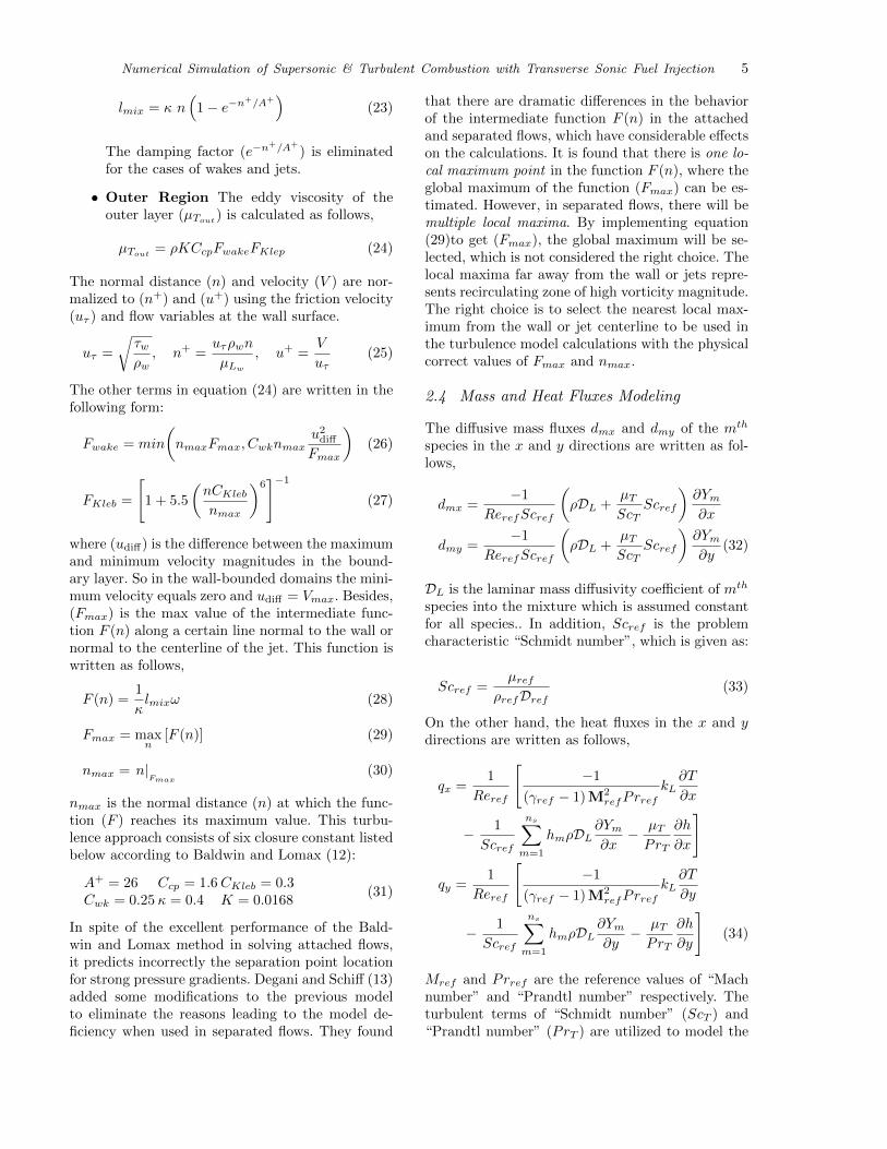
For each of the two cases, three di↵erent sets ofcalculations using di↵erent meshes, whose sizes are31⇥ 51, 61⇥ 51 and 91⇥ 51. They have di↵erentmesh spacing in the stream-wise direction. The mostrefined mesh is shown in figure (2).

4.1.1 Non-reacting Inlet Flow Test Case

In the first test case the inlet temperature is belowthe ignition threshold of hydrogen-air combustionsystem (1000 [K]). But, it rises after the oblique

shock wave and in the viscous layers near wall sur-face, to become high enough, i.e. (greater than1000 [K]), for combustion initiation. The formedoblique shock is considered as detonation wave, asit is responsible in the reaction excitation and sus-tainability.

Local time-stepping is used for the pseudo time-integration, where CFL number equals to (� = 0.1).It is clear from figure (3) that convergence is at-tained after a relatively few number of iterationsbecause a local time step is used instead of smallerglobal time step.

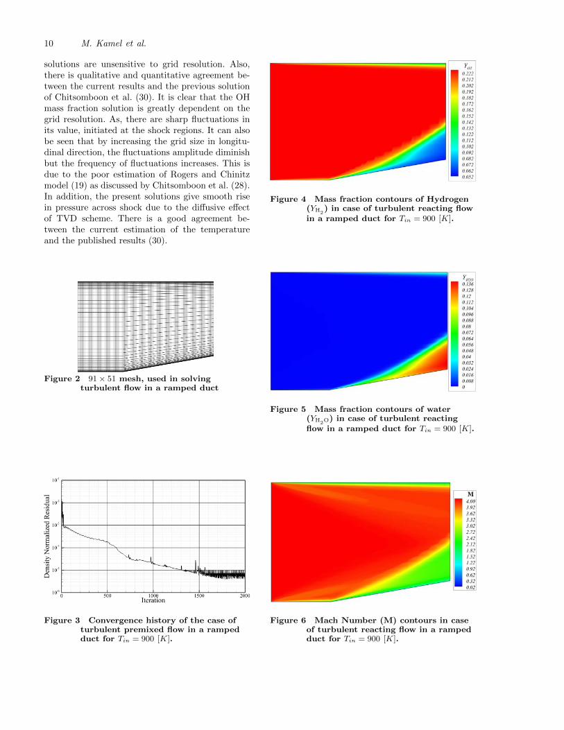
It is clear from figures (4)-(5) that chemical reactionactually begin after the oblique shock wave and inthe shear layer near the lower and upper walls. Asthe inlet temperature is not high enough for com-bustion excitation (i.e. T

in

= 900 [K] < 1000 [K]).Some fluctuation are observable in the Oxygen andHydroxyl mass fractions, along the oblique shockwave. Since, the shock-initiated reactions of O2 ter-mination and OH formation are characterized by itsvery high rates as indicated by Rogers and Chinitzmodel. (19). In figure (6), it obvious that someweek shocks formed at the leading edge of the ductin the lower and upper walls, followed by a strongeroblique shock wave, which reduce flow Mach num-ber (M) about 50% of its value at the duct inlet.Besides, the boundary layer growth is observed,especially at the upper wall, where the boundarylayer thickness reaches its maximum value at theduct exit. The maximum variation in the mixturespecific heat ratio (�

mix

), is about 7.6% relativeto its minimum value, which should be consideredin the evaluation of frozen flow models. The pres-sure and temperature distributions are presented infigures (7) and (8), respectively. There is a rise inthe static pressure following the oblique shock. Itis considered as an evidence of the shock-inducedcombustion e↵ect to increase the static pressure.However, the maximum temperature obtained atthe viscous layers in the lower wall behind theshock, where static temperature is increased to3300 [K], due to the flow deceleration by the shockwave, and due to the shear e↵ect at the adiabaticwalls.

Figures (9)-(14) present the numerical solutionsat the normal distance of 0.13 [cm] from the wall.The present numerical solutions of the three di↵er-ent meshes sizes(31⇥ 51, 61⇥ 51, and 91⇥ 51) arecompared to the previous solutions of Chitsomboonet al. (30), and Shuen and Yoon (22). The present

10 M. Kamel et al.

solutions are unsensitive to grid resolution. Also,there is qualitative and quantitative agreement be-tween the current results and the previous solutionof Chitsomboon et al. (30). It is clear that the OHmass fraction solution is greatly dependent on thegrid resolution. As, there are sharp fluctuations inits value, initiated at the shock regions. It can alsobe seen that by increasing the grid size in longitu-dinal direction, the fluctuations amplitude diminishbut the frequency of fluctuations increases. This isdue to the poor estimation of Rogers and Chinitzmodel (19) as discussed by Chitsomboon et al. (28).In addition, the present solutions give smooth risein pressure across shock due to the di↵usive e↵ectof TVD scheme. There is a good agreement be-tween the current estimation of the temperatureand the published results (30).

Figure 2 91⇥ 51 mesh, used in solvingturbulent flow in a ramped duct

Figure 3 Convergence history of the case ofturbulent premixed flow in a rampedduct for Tin = 900 [K].

Figure 4 Mass fraction contours of Hydrogen(YH2

) in case of turbulent reacting flowin a ramped duct for Tin = 900 [K].

Figure 5 Mass fraction contours of water(YH2O

) in case of turbulent reactingflow in a ramped duct for Tin = 900 [K].

Figure 6 Mach Number (M) contours in caseof turbulent reacting flow in a rampedduct for Tin = 900 [K].


Figure 7 Pressure (P ) contours in case ofturbulent reacting flow in a rampedduct for Tin = 900 [K].

Figure 8 Temperature (T ) contours in case ofturbulent reacting flow in a rampedduct for Tin = 900 [K].

Figure 9 Present solution compared toprevious calculations of ref. (30) and(22) for H2 mass fraction at 0.13 cmfrom the lower wall

Figure 10 Present solution compared toprevious calculations of ref. (30) and(22) for O2 mass fraction at 0.13 cmfrom the lower wall

Figure 11 Present solution compared toprevious calculations of ref. (30) and(22) for OH mass fraction at 0.13 cmfrom the lower wall

Figure 12 Present solution compared toprevious calculations of ref. (30) and(22) for H2O mass fraction at 0.13 cmfrom the lower wall

12 M. Kamel et al.

Figure 13 Present solution compared toprevious calculations of ref. (30) and(22) for pressure at 0.13 cm from thelower wall

Figure 14 Present solution compared toprevious calculations of ref. (30) and(22) for temperature at 0.13 cm fromthe lower wall

4.1.2 Reacting Inlet Flow Test Case

In the second case, when the inlet temperature ex-ceeds the minimum limit of combustion initiation,(i.e. T

in

= 1200 [K] > 1000 [K]), chemical reactionstakes place starting from the duct inlet. However,the static temperature rise at the formed obliqueshock wave accelerates significantly the chemicalreaction rates.

Local time stepping is used for the pseudo time in-tegration with CFL number equals to (� = 0.1). Afast convergence is obtained after 1200 iterations asillustrated in figure (15). The density normalizedresidual is fluctuating below 10�5.

As shown in figures (16)-(17), it is found that thereduction in Oxygen and Hydrogen mass fractions,and the increase in Hydroxyl and water mass frac-tions, start from the duct inlet. However, it is clearthat O2 and H2 termination and OH and H2O

formation are accelerated after the oblique shockwave. The mass fractions of O2 and H2 is reducedafter the shock by about 75% and 50% respectively,relative to their values at the inlet.

It is clear from figure (18) that the waves at theduct leading edges become weaker than that in thefirst case. The variation in flow Mach number (M)before the shock becomes smoother. That is due tothe heat released from the exothermic chemical re-actions initiated at the duct inlet. It is importantto mention that the maximum static pressure at-tained in this problem does not exceed 4.0 [bar],which is lower than that achieved by the previoustest case of lower inlet temperature. Even thoughthe total inlet total pressure is higher in the sec-ond test case, the high static pressure is achievedin the first case. In the first case, the sudden reac-tion initiation across the shock wave in addition ofthe shock compression e↵ect lead to sharp rise instatic pressure only after the oblique shock wave.The thermal energy produced from the exothermicreactions is distributed in smaller region.

Figures (21)-(25) present the numerical solutionsfor three di↵erent meshe sizes, where the discretiza-tion in y-direction is constant (i.e. jmax = 51),and the mesh sizes in x-direction are imax =31, 61, and 91. The solutions are presented at adistance of 0.13 [cm] from the lower wall. The re-sults are compared with the previous results ofYee and Shinn (33) and that of Shuen and Yoon(22). The species concentrations are presented infigures (21)-(23), where there is a sudden decreasein Oxygen and Hydrogen mass fraction, and verysteep rise in Hydroxyl concentration at the duct in-let. The results of O2 and OH concentrations aregreatly a↵ected by the grid resolution at the ductinlet. However, there is a good agreement betweenthe present solution and that of Yee and Shinn(33). In figure (25), the solution of Shuen and Yoon(22), has non-physical oscillations after the shock.The present results and the results of ref. (33) haveno oscillation due to the di↵usive e↵ect of the TVDschemes. In figure (26), there is about 20 % varia-tion between the present solution and that of ref.(22).


Figure 15 Convergence history of the case ofturbulent premixed flow in a rampedduct for Tin = 1200 [K].

Figure 16 Mass fraction contours of Hydrogen(YH2


Figure 17 Mass fraction contours of water(YH2O


Figure 18 Mach number (M) contours in caseof turbulent reacting flow in a rampedduct for Tin = 1200 [K].

Figure 19 Pressure (P ) contours in case ofturbulent reacting flow in a rampedduct for Tin = 1200 [K].

Figure 20 Temperature (T ) contours in case ofturbulent reacting flow in a rampedduct for Tin = 1200 [K].

14 M. Kamel et al.

Figure 21 Present solution compared toprevious calculations of ref. (33) and(22) for H2 mass fraction at 0.13 cmfrom the lower wall

Figure 22 Present solution compared toprevious calculations of ref. (33) and(22) for O2 mass fraction at 0.13 cmfrom the lower wall

Figure 23 Present solution compared toprevious calculations of ref. (33) forOH mass fraction at 0.13 cm from thelower wall

Figure 24 Present solution compared toprevious calculations of ref. (33) and(22) for H2O mass fraction at 0.13 cmfrom the lower wall

Figure 25 Present solution compared toprevious calculations of ref. (33) and(22) for pressure at 0.13 cm from thelower wall

Figure 26 Present solution compared toprevious calculations of ref. (22) fortemperature at 0.13 cm from the lowerwall

4.2 Mixing and Combustion Processes inSingle-Strut Scramjet Engines

Non-reacting and reacting turbulent flow field in a2D single strut scramjet engine model problem are


simulated in this study to investigate the e↵ect ofthe transverse sonic fuel injection on the scramjetengine performance. The configuration of the prob-lem is described in figure (27) as introduced byDrummond and Weidner (26). The engine length is0.78 [m], while its width at the inlet is 0.15 [m].The middle fuel injection strut is 0.258 [m] long andit is centered around the module minimum cross-section, which is located at 0.378 [m] from the in-let leading edge. The half inclination angles of theinjection-strut walls are 7.1 degrees. This geome-try is a two-dimensional projection for an individualmodule of an actual scramjet engine design. Super-sonic air flow enters from the intake, where gaseousHydrogen is injected transversely at sonic speedsfrom four ports at the middle injection-strut locatedat 0.06 [m] downstream from the minimum cross-section. The injection opening taken to be 0.1 [cm]such that the overall equivalence ratio of air- hydro-gen mixture is one. The inlet conditions of both airand Hydrogen are given as follows,

Min

air

= 5.03 Tin

air

= 335.0 [K]Pin

air

= 3546.0 [Pa] TinH2

= 246.0 [K]

PinH2

= 254824.0 [Pa](71)

The longitudinal module length is assumed to be thereference length (L

ref

), while the air inlet proper-ties is used for the other reference variables as givenbelow,

Lref

= 0.78 [m] ⇢ref

= ⇢in

air

Tref

= Tin

air

Vref

= Vin

air

µref

= µL

in

air

kref

= kL

in

airDref

= DL

in

air

(72)

Only the upper half of the scramjet model is con-sidered in the simulation and symmetrical bound-ary conditions are applied at the engine centerline.Meshes of sizes 87⇥ 31 and 200⇥ 51, are employedfor domain discretization. The second mesh is shownin figure (28). The grid lines are clustered near thewall surface and around the vertical line (x = x

o

=0.378 [m]) at which Helium is injected from thelower wall. The governing equations are integratedin time using the global and minimum value of timestep with CFL number of 0.1. Time stepping is notapplied in this case as suggested by Chitsomboon etTiwari (28).

4.2.1 Non-reacting Turbulent Flow Case

By isolating the e↵ect of the chemical reaction onthe flowfield inside the scramjet engine module, thesimulation demonstrates the role of shock systemand recirculation zones created around the trans-verse injection in the mixing process and flame

holding. The distribution of Hydrogen mass frac-tion in that case is used as an to monitor themixing enhancement using transverse injection.In addition, the static temperature distributionin the non-reacting case is examined to find thecombustion-stabilization zones upstream the injec-tors. Two opposite injectors are placed near theminimum cross-section of the engine in order toguarantee e↵ective mixing process. Also, the mix-ing is enhanced by raising the injection pressurerelative to the air flow to force the fuel penetrationinto the supersonic main flow. The injection pres-sure is about 70 times the air flow static pressure.

As shown in figures (29)-(30) for a mesh size of200⇥ 51. Recirculation zone is created in the engineintake due to shock-wave/boundary-layer inter-actions. Mach number contours show clearly anoblique shock wave originated from the intake lead-ing edge then reflected at the middle strut apex tothe upper wall. Shock wave reflection creates a rel-atively high speed recirculation zone. Then the flowgoes through complicated system of shock reflec-tion and separation shock at the module minimumcross-section. The shock waves deflects airflow di-rection parallel to the injection strut walls leadingto large vortical zone adjacent to the engine wall.The upstream vortical flow speed is higher thanthat of the other downstream recirculation zoneswhich leads to static temperature increase up to2300[K] in the turbulent shear layers as shown infigure (32). The recirculation zone, upstream of theinjector at the middle strut wall, extends upstreamto pass through the minimum cross-section. H2-airmixing is carried out in the vortical flow front ofthe injection region, as illustrated in figure (31).After the injection region, the mixture is then ex-panded, where Hydrogen di↵usively transfers intoair as mixing layers.

The solutions of the two mesh sizes (87⇥ 31 and200⇥ 51) are compared to each other. Comparisonsare carried out in terms of normalized variablesto facilitate the evaluation of the di↵erent sets ofresults. The utilized normalized variables are theaxial and transversal normalized distance; x

norm

,and y

norm

respectively, in addition to the nor-malized pressure (P

norm

). They are expressed asfollows,

xnorm

=x� xintake leading edge

xintake leading edge � xnozzle trailing edge

ynorm

=y � y

min

ymax

� ymin

(73)

16 M. Kamel et al.

The results of the non-reacting case at di↵erent sta-tions upstream and downstream the injection portsfor mesh sizes of 87⇥ 31 and 200⇥ 51 are com-pared with the previous calculations. Solutions ofH2 mass fraction, and static temperature, at dif-ferent axial normalized distances are presented infigure (33) and (34). Stations of axial normalizeddistance ranging between 0.51 and 0.55 representthe flow domain upstream the injection ports, whilethose ranging between 0.57 and 0.61 represent thedownstream flowfield.

The solutions of 87⇥ 31-sized mesh underestimatethe H2 mass fraction upstream the injection port.Refining the mesh to a size of size 200⇥ 51 enablesto predict accurately the flowfield as shown in theresults of the Hydrogen mass fraction. The 200⇥ 51results show that H2-air mixing is more e↵ectiveat the module wall than that at the middle strutsurface because larger size of the recirculation zoneformed adjacent to the upper wall as presented infigure (30).

Based on the simulation results for the non-reactingcase, it is clear that there are recirculation zonesof low speed and high temperature are created up-stream the injection ports. And that helps in theflame self-ignition and stabilization for supersoniccombustion. Also, the fuel-air mixing is improved,as the shocks created upstream the injector decel-erate the incoming supersonic air flow, in order tobe turbulently mixed with injected hydrogen in thetransverse direction.

4.2.2 Reacting Turbulent Flow Case

The unsteady Navier-Stocks equations are solvedusing a minimum time step with CFL number of0.1. A system of equations composed of eight cou-pled non-linear partial di↵erential equations aresolved. Four reacting species (i.e. O2, H2, OH, andH2O) are considered in the simulation while Nitro-gen is assumed to be inert.

A mesh size of 200⇥ 51 is used in the simulationof the reacting and turbulent H2-air flow insidescramjet engine, which is the greater than the meshsize employed in Drummond and Weidner (26), andChitsomboon et al. (29). The results of this simu-lation are presented in figures (35)-(39). It is clearfrom the results that the recirculation zones up-stream the minimum cross-section becomes largercompared to the non-reacting case due to the in-crease in the static temperature inside the injectionzone. The static temperature is raised to 3300 [K]

approximately in the flow-separation region up-stream the injectors. Static temperature increasesclose to the impact zone of the vortex flow withperpendicular H2 injection.

Hydrogen mass fraction is nearly zero in the frontof the recirculation zones and it is also reduced inthe free mixing layer along the engine module asshown in figure (38) which indicates to an enhance-ment of the mixing and flame-holding processes dueto the formation of these vortical structures. Themagnitude of water mass fraction demonstratesthe extent of the combustion along the flow field.Combustion is mainly initiated and sustained bymeans of the separating shocks in front of the in-jected H2 stream as shown in figure (37). It is clearfrom figure (39), that the flame-holding recircula-tion zones have simpler eddy-structure comparedto the non-reacting test case because the separa-tion intensity is diminished as a result of the totaltemperature increase in the combustion zone.

In figures (43) and (41) present the solutions oftemperature and water mass fraction at di↵erentstream-wise stations in the engine. They are qual-itativaly compared with the previous solutions ofChitsomboon et al (29) shown in figure (42) and(44). Point-to-point comparison is unavailable, be-cause the x-stations coordinates are not given inref. (29).

As illustrated in figures (42) and (41), the H2Omass fraction solution of the 87⇥ 31-sized meshof Chitsomboon et al. (29), is less than predictedby the present solution utilizing 200⇥ 51-sizedmesh. It is noted that the magnitude of H2O doesnot significantly change as an indication of fuel-air mixing e�ciency in the recirculation zones.In addition, qualitative analysis between the nor-malized temperature of previous solution and thestatic temperature of the present solution showsresemblance in temperature field downstream theinjectors While the present solution predicts almostconstant static temperature in the front recircula-tion zones.

The results of the normalized pressure on the engineupper wall surface are compared with the calcula-tions of Chitsomboon et al. (29). In figure (45), thenormalized pressure is presented along the wholeengine module, where the normalized pressure forall solutions equal to unity at the injection zone.The previous solution of the reacting case agreeswith the non-reacting solution of the same mesh


size (87⇥ 31). The normalized pressure is given asfollow,

Pnorm

=P � Pair inlet

PH2 injection � Pair inlet(74)

Figure 27 Schematic diagram for singletwo-dimensional strut Scramjet Engine

Figure 28 200⇥ 51 mesh, used in solvingturbulent 2D flow in single strutscramjet engine

Figure 29 Mach number (M) contours of thenon-reacting case solution, for meshsize 200⇥ 51

Figure 30 Mach number (M) contours withinthe upper injection zone, for thenon-reacting case solution, for meshsize 200⇥ 51

Figure 31 Hydrogen mass fraction (YH2)

contours of the non-reacting casesolution, for mesh size 200⇥ 51

Figure 32 Temperature (T ) contours of thenon-reacting case solution, for meshsize 200⇥ 51

Hydrogen Mass Fraction (YH2)

Hydrogen Mass Fraction (YH2)

Nor

mal

ized

Tra

nsve

rsal

Dis

tanc

e

(ynorm

)N

orm

aliz

ed T

rans

vers

al D

ista

nce

(y

norm

)

0 0.5 10

0.5

1xnorm= 0.51

0 0.5 10

0.5

1xnorm= 0.53

0 0.3 0.6 0.90

0.5

1xnorm= 0.57

0 0.5 10

0.5

1xnorm= 0.55

0 0.5 10

0.5

1xnorm= 0.57

0 0.5 10

0.5

1xnorm= 0.58

0 0.5 10

0.5

1xnorm= 0.59

0 0.5 10

0.5

1xnorm= 0.61

0 0.5 10

0.5

1xnorm= 0.52

0 0.5 10

0.5

1xnorm= 0.54

0 0.5 10

0.5

1xnorm= 0.60

Figure 33 Hydrogen mass fraction solution atdi↵erent station, for the non-reactingcase for mesh size 200⇥ 51

18 M. Kamel et al.

Temperature (T) [K]

Temperature (T) [K]Nor

mal

ized

Tra

nsve

rsal

Dis

tanc

e

(ynorm

)N

orm

aliz

ed T

rans

vers

al D

ista

nce

(y

norm

)

0 1000 20000

0.5

1xnorm= 0.53

0 0.3 0.6 0.90

0.5

1xnorm= 0.57

0 1000 20000

0.5

1xnorm= 0.55

0 1000 20000

0.5

1xnorm= 0.57

0 1000 20000

0.5

1xnorm= 0.58

0 1000 20000

0.5

1xnorm= 0.59

0 1000 20000

0.5

1xnorm= 0.60

0 1000 20000

0.5

1xnorm= 0.61

0 1000 20000

0.5

1xnorm= 0.52

0 1000 20000

0.5

1xnorm= 0.54

0 1000 20000

0.5

1xnorm= 0.51

Figure 34 Temperature solution at di↵erentstation, for the non-reacting case formesh size 200⇥ 51

Figure 35 Mach number (M) contours of thereacting case solution, for mesh size200⇥ 51

Figure 36 Temperature (T ) contours of thereacting case solution, for mesh size200⇥ 51

Figure 37 Water mass fraction (YH2O) contours

of the reacting case solution, for meshsize 200⇥ 51

Figure 38 Hydrogen mass fraction (YH2)

contours of the reacting case solution,for mesh size 200⇥ 51

Figure 39 Mach number (M) contours withinthe upper injection zone, for thereacting case solution, for mesh size200⇥ 51

Figure 40 Water mass fraction (YH2O) contours

within the upper injection zone, for thereacting case solution, for mesh size200⇥ 51


Figure 41 Water mass fraction solution atdi↵erent station, for the reacting casefor mesh size 200⇥ 51

Figure 42 Previous solution for water massfraction at di↵erent station, for thereacting case (ref. (29))

Figure 43 Temperature solution at di↵erentstation, for the reacting case for meshsize 200⇥ 51

Figure 44 Previous solution for normalizedtemperature at di↵erent station, forthe reacting case (ref. (29))

Figure 45 Normalized pressure solution on theupper wall, compared to the previoussolution (ref.(29))

5 Conclusion

Development of scramjet engines of satisfactory per-formance requires enhancement of the fuel-air mix-ing and flame stabilization. The e↵ect of transversesonic fuel injection on fuel-air mixing and flamestabilization is investigated numerically in the cur-rent study. A numerical tool is developed using theReynolds Average Navier-Stokes equations. Chem-ical kinetics model is employed to compute the fi-nite rates of the chemical reactions. Zero-equationof Baldwin-Lomax are used to calculate the turbu-lent eddy viscosity. Finite-volume scheme is appliedwhere the convective fluxes are discretized by sec-ond order accurate Roe’s scheme using MUSCL ap-proach. Second order accurate Runge-Kutta methodis used for the time-integration. The convective andviscous flow fluxes are treated explicitly, where only

20 M. Kamel et al.

the chemical source term is solved implicitly in or-der to reduce the computational e↵orts of invertingthe flow Jacobians. The problem of Helium trans-verse sonic injection into supersonic air flow is sim-ulated and the results are compared with the pre-vious investigations. In addition, air-hydrogen flowis studied in a single strut scramjet engine, wheremixing and flame holding processes are carried outusing fuel transverse sonic injection. The simulationshows that high adverse pressure gradient is creatednear the injection zone. Thus, a separation shock isformed with a recirculation zone in front of the injec-tion region and the combustion process is sustained.The results are compared with previous numericaland experimental investigations and the results arein good agreement with the published data.

References

[1] J. P. Drummond, J. P. (1979). “Numerical In-vestigation of the Perpendicular InjectorFlow Field in a Hydrogen Fueled Scram-jet”, J. P. Drummond, NASA Langley ResearchCenter, Hampton, Va. AIAA 12th FLUID ANDPLASMA DYNAMICS CONFERENCE July 23-25, 1979 / Williamsburg,Virginia

[2] Farshchi, M., “Supersonic Turbulent React-ing Flow Modeling and Calculation”, Tech-nical Report NASA-CR-196185, National Aero-nautics & Space Administration, Lewis ResearchCenter, April 1991.

[3] Drummon d, J. P.; Rogers, R. C.; and Evans, J.S. , “Combustor Modeling for Scramjet En-gines”, AGARD CP 275. Presented at AGARDCombustor Modeling, Cologne, Oct. 1979.

[4] Cinnella, P. and Grossman, B., “Computa-tional Methods for Chemically ReactingFlows”, Handbook of Fluid Dynamics and FluidMachinery, Wiley and Sons, New York, 1996, pp.1541“1590.

[5] Spalart, P. R.; Jou, W. H.; Strelets, M.; andAllmaras, S. R., “Comments on the Feasi-bility of LES for Wings, and on a HybridRANS/LES Approach”, In 1st AFOSR Inter-national Conference on DNS/LES, Aug. 1997.

[6] Tannehill, J.C.; Anderson, D.A.; and Pletcher,R.H., “Computational Fluid MechanicsAnd Heat Transfer”, Second Edition, pub-lished by Taylor & Francis Ltd., London, UK,1997.

[7] Chou, P. Y., “On the Velocity Correlationsand the Solution of the Equations of Tur-bulent Fluctuation”, Quart. Appl. Math., Vol.3, p.38.

[8] Davidov, B.I., “On the Statistical Dynam-ics of an Incompressible Fluid”, Doklady AN.SSSR, Vol. 136, p. 47.

[9] Kolmogorov, A. N., “Equations of turbulentMotion of an Incompressible Fluid”, IsvestiaAcademy of Sciences, USSR; Physics, Vol. 6, No.1 and 2, pp. 56�58.

[10] Baldwin, B.S. and Barth, T.J., “A One-Equation Turbulence Transport Model forHigh Reynolds Number Wall-BoundedFlows”, NASA Technical Memorandum-102847,1991.

[11] Smith, A.M.0. and Cebeci, T., “NumericalSolution of the Turbulent Boundary-LayerEquations”, Douglas Aircraft Division ReportDAC 3373.

[12] Baldwin , B.S. and Lomax, H., “Thin LayerApproximation and Algebraic Model forSeparated Turbulent Flows”, AIAA Paper78�257, 16th Aerospace Sciences Meeting, Jan-uary 1978.

[13] Degani, D. and Schi↵, L.B., “Computation ofSupersonic Viscous Flows Around PointedBodies at Large Incidence” AIAA Paper83�0034, AlAA 21st Aerospace Sciences Meeting,January 1983.

[14] Mottura, L.; Vigevano, L., and Zaccanti, M.(2000). “Factorized Implicit Upwind Meth-ods Applied to Inviscid Flows at HighMach Number”, AIAA Journal, Vol. 38, No.10, October 2000.

[15] Yoon, S., and Jameson, A., “Lower-UpperSymmetric Gauss-Seidel Method for Eulerand Navier-Stocks Equations”, AIAA Jour-nal, Vol. 26, No. 9, pp. 1025�1026, September1988.

[16] Curtiss, C.F. and Hirschfelder, J.O., “Inte-gration of Sti↵ Equations”, Proc. NationalAcademy of Sciences of the USA, Vol. 38, 1952.

[17] Grossman, B. and Cinnella, P., “Flux-Split Algorithms For Flows WithNon�Equilibrium Chemistry And Vibra-tional Relaxation”, Journal of ComputationalPhysics 88, pp. 131�168, 1990.


[18] Walters, R.W.; Cinnella, P.; Slack, D.C.; andHalt, D., “Characteristic�Based Algorithmsfor Flows in Thermo�Chemical Nonequi-librium”, AIAA Paper 90�0393, 28th AerospaceSciences Meeting, January 1990.

[19] Rogers, R.C. and Chinitz, W., “Using aGlobal Hydrogen�Air Combustion Modelin Turbulent Reacting Flow Calculations”,AIAA Journal Vol. 21, No. 4, pp. 586�592, April1983.

[20] (a) Bussing, T.R.A. and Murman, E.M., “AFinite Volume Method For The Calcula-tion of Compressible Chemically ReactingFlows”, AlAA Paper 85�0331, 23rd AerospaceSciences Meeting, January 1985.

[21] (b) Bussing, T.R.A. and Murman, E.M., “Nu-merical Investigation of 2�DimensionalH2 �Air Flame Holding Over RampsAnd Rearward Facing Steps”, AIAA Paper85�1250, 21st Joint Propulsion Conference, July1985.

[22] Shuen, J.S. and Yoon, S., “Numerical Studyof Chemically Reacting Flows Using an LUScheme”, AIAA Journal, Vol. 27, No. 12, pp.1752�1760, December 1989.

[23] Hitch, B.D.; Laxter, W.R.; Senser, D.W.; andSojka, P.E., “On the Selection of H2/AirKinetic Mechanisms for Use in Super-sonic Combustor Modeling”, presented at theSpring 1986 Technical Meeting of the CentralStates Section of the Combustion Institute, May1986.

[24] Eklund, D. R.; Hassan, H. A.; and Drummond,J. P., “Time E�cient Calculation of Chem-ically Reacting Flow”, AIAA Paper No. 86-0563, January 1986.

[25] Drummond, J.P.; Hussaini, M.Y. and Zang,T.A., “Spectral Methods for ModelingSupersonic Chemically Reacting FlowFields”, AlAA Paper 85�0302, 23rd AerospaceSciences Meeting, January 1985.

[26] Drummond, J.P. and Weidner, E.H. , “Nu-mericalS tudy of a Scramjet Engine FlowField”, AlAA 19th Aerospace Sciences Meeting,January 1981.

[27] Chitsomboon, T. and Tiwari, S. N., “Investi-gation of Chemically Reacting SupersonicInternal Flows”, Department of Mechanical

Engineering and Mechanics, School of Engineer-ing, Old Dominion University. Technical Report,NAG-1-423, September 1985.

[28] Chitsomboon, T. and Tiwari, S.N., “Numer-ical Study of Hydrogen�Air SupersonicFlow By Using Ellipitic And ParabolizedEquations”, Progress Report for the period De-cember 1 1985 to May 31 1986, Prepared forNASA, Langley Research Center, Hampton, Vir-ginia, USA, August 1986.

[29] Chitsomoon, T.; Kumar, A.; Drummond, J.P.and Tiwari, S.N., “Numerical Study of Su-personic Combustion Using A Finite�RateChemistfw Model”, AlAA Paper 86�0309,24th Aerospace Sciences Meeting, January 1986.

[30] Chitsomboon, T.; Kumar, A. and Tiwari, S.N.,“Numerical Study of Finite�Rate Super-sonic Combustion Using Parabolized Equa-tions”, AIAA Paper 87�0088, 25th AerospaceSciences Meeting, January 1987.

[31] McBride, B.J.; Gordon, S. and Reno, M.R.,“Coe�cients for Calculating Thermody-namic and Transport Properties of Individ-ual Species”, NASA Technical Memorandum4513, October 1993.

[32] Roe, P.L., “Approximate RiemannSolvers, Parameter Vectors, and Di↵er-ence Schemes”, Journal of ComputationalPhysics, Vol. 43, No. 2, pp. 357�372, October1981.

[33] Yee, H.C. and Shinn, J.L., “Semi-Implicitand Fully Implicit Shock-Capturing Meth-ods for Hyperbolic Conservation Laws withSti↵ Source Terms”, 8 th Computational FluidDynamics Conference, AIAA, New York, 1987,pp. 159-176. (NASA Technical Memorandum–89415).

[34] Anderson, J.D., “Hypersonic and HighTemperature Gas Dynamics”, American In-stitute of Aeronautics and Astronautics Inc., Re-ston, Virginia, USA, 2006.

numerical simulation of supersonic and turbulent ...mkamel/publications/mkamel-ijesms-2015-7_… ·...

Documents