numerical simulation of one dimensional heat equation: · pdf filenumerical simulation of one...

Numerical Simulation of one dimensional Heat Equation: B-Spline Finite

Element Method

V.Dabral. Department of Mathematics

Roorkee Institute of Technology, Roorkee-247667

S.Kapoor Department Of Mathematics

Indian Institute Of Technology, Roorkee-247667, India

S.Dhawan Department Of Mathematics

Dr. B.R.Ambedkar National Institute Of Technology, Jalandhar-144011 (Punjab), India

Abstract

The comprehensive numerical study has been made here for the solution of One dimensional heat equation the Finite Element method is adopted for the solution with B-spline basis function the important finding of the present study is to understand the basics behind the FEM method while the B-spline basis function come into the picture here the solution is made using Quadratic B-spline and Cubic B-spline. Then for both the cases the solution is compare with analytical solution in which a good agreement is found between proposed technique. Along with that the simulation process is made using MATLAB programming in which the 3-Dimensional geometrical intrepitaion shown as a graphical presentation taken a different time steps as well as different domain of interest , the dirichlet boundary condition has been taken for the solution of this problem which is again a good achievement of the above work along with two test problem has been taken for the sake of convince. Finally the goal has been achieved in a simulation process. Keywords; Quadratic B-spline, Cubic B-spline, FEM, Stability, Simulation, MATLAB Introduction

HEAT equation is a simple second-order partial differential equation that describes the variation temperature in

a given region over a period of time. In this work, suppose the heat flows through a thin rod which is perfectly

insulated along its length except at the two ends, its position in the rod is denoted as x where 0 ≤ x ≤ 1 and the

length of the rod is represented as L, as illustrated in Fig. A.

Figure A schematic diagram of temperature variation in a heated road.

, = , Ω × [0, ] Where is the thermal conductivity (1)

Where Ω = [0, ], with initial condition

, 0 = 0 ≤ ≤ , (2)

And the boundary conditions

0, = 0 ≤ ≤ , (3)

, = 0 ≤ ≤ , (4)

where , , are density, thermal conductivity in the direction of x-axis and heat capacity respectively. , ,

are known functions and , is unknown. Its a well-known second order linear partial differential

V.Dabral et al. / Indian Journal of Computer Science and Engineering (IJCSE)

ISSN : 0976-5166 Vol. 2 No. 2 Apr-May 2011 222

equation(PDE). Unlike other equations, it is not preserved when t is replaced by -t. It shows that heat equation

describes ir reversible process and makes a distance between the previous and next steps. Such equations arise

very often in various applications of science and engineering describing the variation of temperature (or heat

distribution) in a given region over some time. Heat equation mainly in one-dimension had been studied by

many authors as in references therein [1], [2], [8], [9]. An comparative study between the traditional separation

of variables method and Adomian method for heat equation had been examined by Gorguis and Benny Chan

[5]. Dehghan [4] considered the use of second-order finite difference scheme to solve the two-dimensional heat

equation. After that, Mohebbi and Dehghan [2] presented a fourth-order compact finite difference approximation

and cubic -spline collocation method for the solution with fourth-order accuracy in both space and time

variables, ℎ"#". In literature [7], Kumar concluded that spline gives a simple and practical method to solve

the boundary problems compared to finite difference method. On the other hand, an extension of B-spline

function, namely extended cubic uniform B-spline had been proposed by Han and Liu in literature [6].

In contrast to the heat equation, the steady sate constant is not simply the integral of the initial condition, but

also depends in some complicated way on both the viscosity parameter and the shape of the initial condition,

cf.,[11] in particular, numerical calculations have been used to “suggest” that Euler equations do not have

unique solution, cf., [12]. The justification for this claim is that a “very fine mesh” is used in the calculation. In

this note we suggest that “numerical based” proofs of non-existence must be done with extreme care.problem

which arises in the quasi-static theory of thermoelasticity (Day [13], [14]). Investigators like Ekolin [15] and Liu

[16] had studied the problem and introduced finite-difference methods for solving it numerically. The numerical

solution of the heat equation is discussed in many textbooks. Ames [18], Morton and Mayers [20], and Cooper

[17] provide a more mathematical development of finite difference methods. See Cooper [17] for modern

introduction to the theory of partial differential equations along with a brief coverage of numerical methods.

Fletcher [19], Golub and Ortega [21], and Homan [22] take a more applied approach that also introduces

implementation issues. Fletcher provides Fortran code for several methods.Marwaha & Chopra [26] give a

numerical solution for transient thermal distribution in a slab where chemical, electrical or nuclear energy is

converted into thermal energy. To describe temperature profile, Elimoel and Rogerio [27] uses exponential-

sinusoidal one-dimensional analytical model demonstrating that heat equation can still be solved analytically.

Monte [28] applied a natural analytical approach for solving the one dimensional transient heat conduction in a

composite slab. He studied the transient response of one dimensional multilayered composite conducting slabs

to the sudden variations of the temperature of surrounding fluid. In a one dimensional hollow composite

cylinder with time dependent boundary conditions, Lu [29] gave a novel analytical method applied to the

transient heat conduction equation.

Splines are a kind of piecewise polynomials that are easy to use for the approximations by breaking an

interval into a number of subintervals [30]. In general, we consider a piecewise polynomial, let [a, b] be a f inite

interval and < , … . . , < ' be the partition of [a,b] into n elements and (; (i = 0,1,…n) are the nodes.

These nodes are the parameter values where the polynomial function constituting spline curve joining each other

[31]. A particular class of splines are - B-splines. B-spline (bell-shaped splines) are piecewise polynomial

functions that are connected continuously by the smaller curve segments that takes care of the continuity having

a direct impact on the basis functions. B-spline functions are very popular for the smooth approximations and

are being used by various researchers for different problems ([32], [33] , [34], [35],[36]). In 1946, Schoenberg

first proposed the theory of B-splines. Cox(1971) and de Boor(1972) gave recurrence relations for the purpose

of computing coefficients ([37], [38]). Yang [39] used a technique to deal with the boundary conditions using

splines. Many others [40], [41] has used B-splines for various applications where B-splines has been proved a

useful tool for approximations. In addition to this Thomas [42] presented extensive use of splines for Boeing.

Qiu [43] applied a trivariate B-spline fo r volume reconstruction saying that the B-spline reconstructions are

often superior to the existing methods. In the present method we proposed a cubic B-spline FEM for the solution

of one dimensional heat conduction equation. Because B-spline curve has superior properties making them

suitable for shape representations and analysis purpose. Using the values of B-splines, nodal values at the knots

are expressed in terms of the element parameters. Temperature distribution over the subintervals will be

approximated by the combination of cubic B-splines and unknown element parameter. The system is reduced to

the matrix form and further handled by method of lines. Simulation ,etc



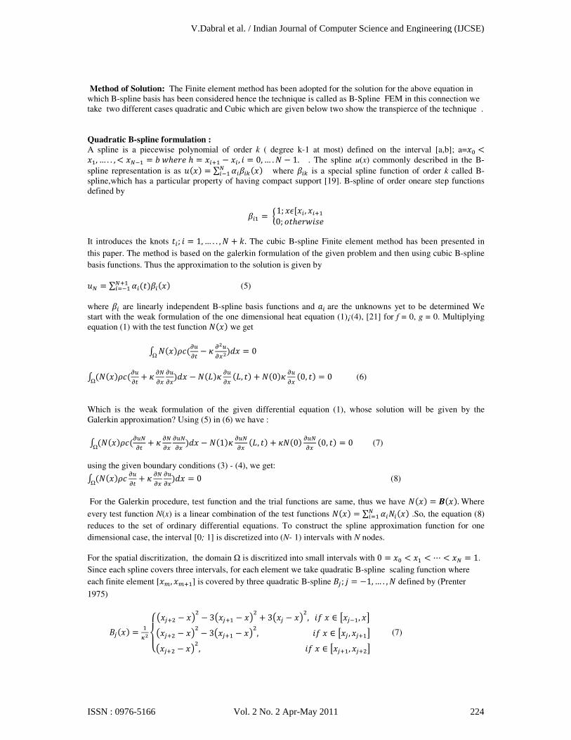
Method of Solution: The Finite element method has been adopted for the solution for the above equation in which B-spline basis has been considered hence the technique is called as B-Spline FEM in this connection we take two different cases quadratic and Cubic which are given below two show the transpierce of the technique . Quadratic B-spline formulation :

A spline is a piecewise polynomial of order k ( degree k-1 at most) defined on the interval [a,b]; a= <, … . . , < ') = *+ℎ,,ℎ = (- − ( , / = 0,… .0 − 1. . The spline u(x) commonly described in the B-spline representation is as = ∑ 3((4'() where (4 is a special spline function of order k called B-spline,which has a particular property of having compact support [19]. B-spline of order oneare step functions defined by

( = 51; [( , (-0; ℎ,+/7,8 It introduces the knots (; / = 1,… . . , 0 + #. The cubic B-spline Finite element method has been presented in

this paper. The method is based on the galerkin formulation of the given problem and then using cubic B-spline

basis functions. Thus the approximation to the solution is given by

' = ∑ 3(('-(:) (5)

where ( are linearly independent B-spline basis functions and ;( are the unknowns yet to be determined We start with the weak formulation of the one dimensional heat equation (1)¡(4), [21] for f = 0, g = 0. Multiplying equation (1) with the test function 0 we get

< 0=>=Ω

− =?>=?@ = 0

< 0=>=Ω

+ ='= =>=@ − 0 =>= , + 00 =>= 0, = 0 (6)

Which is the weak formulation of the given differential equation (1), whose solution will be given by the Galerkin approximation? Using (5) in (6) we have :

< 0=>'=Ω

+ ='= =>'= @ − 01 =>'= , + 00 =>'= 0, = 0 (7)

using the given boundary conditions (3) - (4), we get: < 0 =>=Ω

+ ='= =>=@ = 0 (8)

For the Galerkin procedure, test function and the trial functions are same, thus we have 0 = A.Where

every test function N(x) is a linear combination of the test functions 0 = ∑ 3(0('(: .So, the equation (8)

reduces to the set of ordinary differential equations. To construct the spline approximation function for one

dimensional case, the interval [0; 1] is discretized into (N- 1) intervals with N nodes.

For the spatial discritization, the domain Ω is discritized into small intervals with 0 = < < ⋯ < ' = 1.

Since each spline covers three intervals, for each element we take quadratic B-spline scaling function where

each finite element [C, C-] is covered by three quadratic B-spline DE ; F = −1,… . , 0 defined by (Prenter

1975)

DE = G?HIJKE- − L − 3KE- − L + 3KE − L,/ ∈ OE), PKE- − L − 3KE- − L,/ ∈ OE , E-PKE- − L,/ ∈ OE-, E-P

8 (7)



The length of each interval E − E) = for all i and each interval is covered by three successive quadratic B-

splines. DE ; F = −1,… . , 0 and its first derivative vanish outside the interval [E), E-]. Integrating PDE by

psrts we get

Approximate in term of basis function wedefines

(', = Q 3EE'

E:)

Where DE are quadratic B-splines basis function in given equation and 3E ;,unkown . The approximation ('

and its first derivative is continuous across the solution domain. Using that the solution can be obtained using

unknowns .

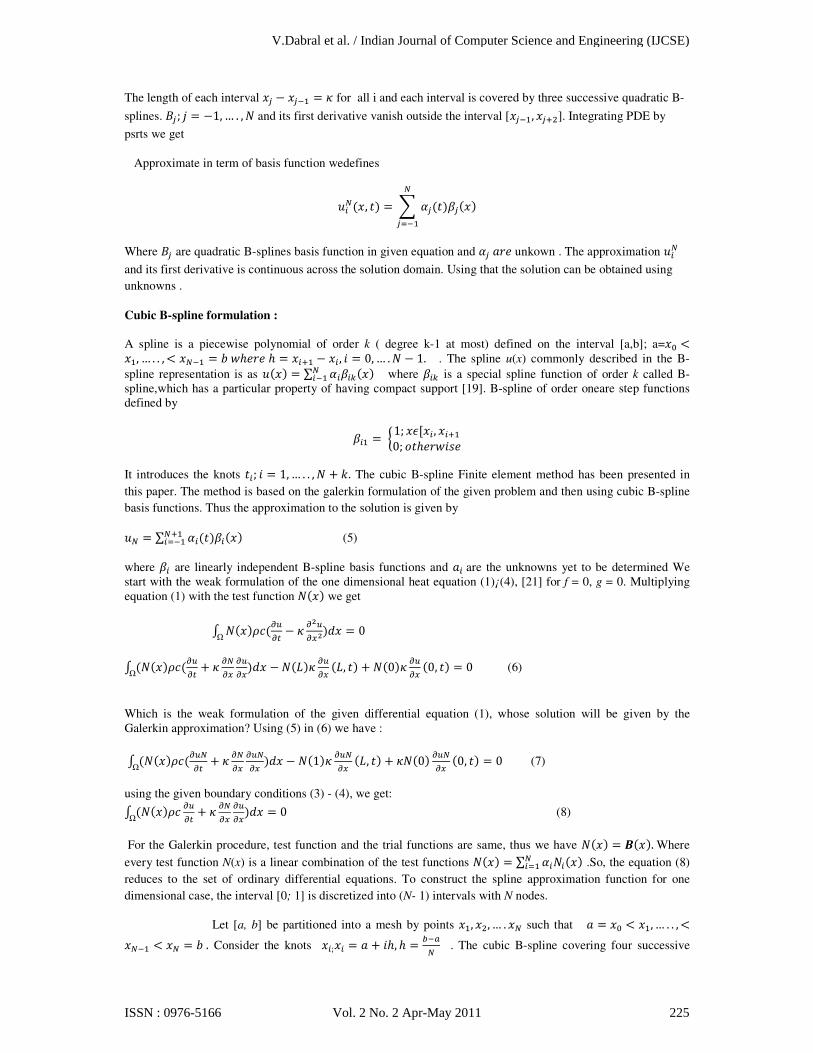
Cubic B-spline formulation :

A spline is a piecewise polynomial of order k ( degree k-1 at most) defined on the interval [a,b]; a= <, … . . , < ') = *+ℎ,,ℎ = (- − ( , / = 0,… .0 − 1. . The spline u(x) commonly described in the B-spline representation is as = ∑ 3((4'() where (4 is a special spline function of order k called B-spline,which has a particular property of having compact support [19]. B-spline of order oneare step functions defined by

( = 51; [( , (-0; ℎ,+/7,8 It introduces the knots (; / = 1,… . . , 0 + #. The cubic B-spline Finite element method has been presented in

this paper. The method is based on the galerkin formulation of the given problem and then using cubic B-spline

basis functions. Thus the approximation to the solution is given by

' = ∑ 3(('-(:) (5)

where ( are linearly independent B-spline basis functions and ;( are the unknowns yet to be determined We start with the weak formulation of the one dimensional heat equation (1)¡(4), [21] for f = 0, g = 0. Multiplying equation (1) with the test function 0 we get

< 0=>=Ω

− =?>=?@ = 0

< 0=>=Ω

+ ='= =>=@ − 0 =>= , + 00 =>= 0, = 0 (6)

Which is the weak formulation of the given differential equation (1), whose solution will be given by the Galerkin approximation? Using (5) in (6) we have :

< 0=>'=Ω

+ ='= =>'= @ − 01 =>'= , + 00 =>'= 0, = 0 (7)

using the given boundary conditions (3) - (4), we get: < 0 =>=Ω

+ ='= =>=@ = 0 (8)

For the Galerkin procedure, test function and the trial functions are same, thus we have 0 = A.Where

every test function N(x) is a linear combination of the test functions 0 = ∑ 3(0('(: .So, the equation (8)

reduces to the set of ordinary differential equations. To construct the spline approximation function for one

dimensional case, the interval [0; 1] is discretized into (N- 1) intervals with N nodes.

Let [a, b] be partitioned into a mesh by points , , … . ' such that ; = < , … . . , <') < ' = *. Consider the knots (;( = ; + /ℎ, ℎ = R)S' . The cubic B-spline covering four successive



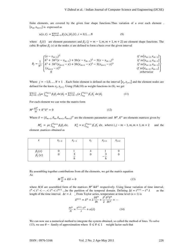
finite elements, are covered by the given four shape functions.Thus variation of u over each element . [C, C-] is expressed as

, = ∑ E(;TEC-E:C) , / = 0,1, …0 (9)

where TE are element parameters and E ; F = U − 1,U,U + 1,U + 2are element shape functions. The cubic B-spline E (x) at the nodes xi are defined to form a basis over the given interval

DE = 1ℎW HXIXJ − C)

W/[C), C)]ℎW + 3ℎ − C) + 3ℎ − C) − 3 − C)W/[C), C)]ℎW + 3ℎC- − + 3ℎC- − − 3C- − W/[C), C)]C- − W/[C), C)]0ℎ,+/7, YXZX[

Where F = −1,0, … . 0 + 1 . Each finite element is defined on the interval OE, E-P and the element nodes are

defined for the knots E , E-. Using (9)&(10) as weight functions in (8), we get

∑ < (E\]^\C-E:C) @TE +∑ < (′ E′ \]^\C-E:C) @TE (11)

For each element we can write the matrix form _` abca + d`T` = 0 (12)

Where T = TC), TC, TC-, TC-e are the elements parameters and _` , d` are elements matrices given by

_(E = < (E\]^\ @, d(E = < (′ E′ \]^\ @, +ℎ,,/, F − U − 1,U,U + 1,U + 2 and the

element ,matrices obtained as

By assembling together contributions from all the elements, we get the matrix equation As _ aba + dT = 0 (13)

where M,K are assembled form of the matrices _` &d` respectively. Using linear variation of time interval, < < ⋯ .< g < g-….be the partition of the temporal domain. Defining ∆ = g- − gi as the length of the time interval. ∆ = i ¸ From Taylor series, temperature at time level (n + 1) is

Tg- = Tg + i jTgj + i2 jTgj +⋯

=bk= ≈ bk]^)bkm + i (14)

We can now use a numerical method to integrate the system obtained, so called the method of lines. To solve (13), we use n − family of approximation where 0 ≤ n ≤ 1 weight factor such that

E) E) E E- E-

E E′

0 0 3ℎ

1 4 0 −3ℎ

1 0 0



Tg-o = nTg- + 1 − nTg (15)

Using (14) and (15) into (13) we have

[_] pTg- − Tgi q +[d]Tg-o = 0

[_] pTg- − Tgi q +[d]nTg- + 1 − nTg = 0

A simple rearrangement given us

_ + nidTg- = _ − i1 − ndTg (16)

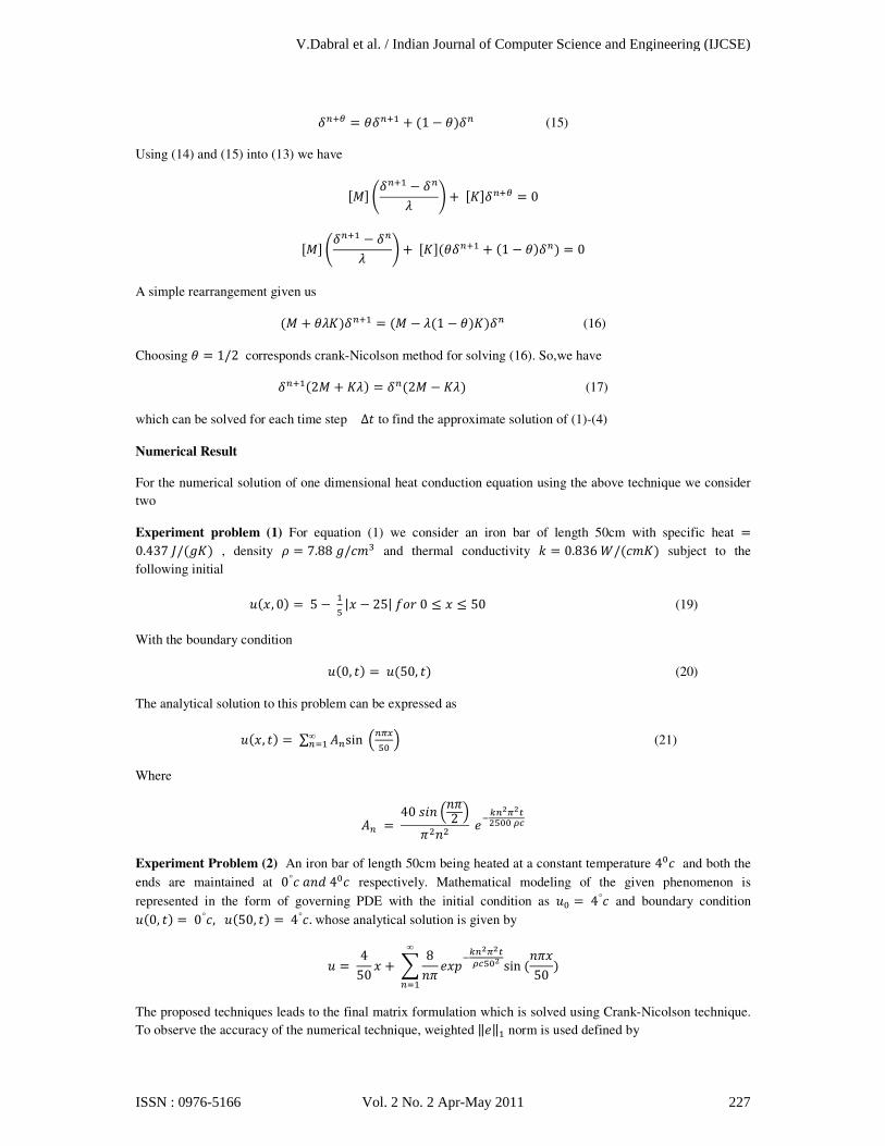
Choosing n = 1/2 corresponds crank-Nicolson method for solving (16). So,we have Tg-2_ + di = Tg2_ − di (17)

which can be solved for each time step ∆ to find the approximate solution of (1)-(4)

Numerical Result

For the numerical solution of one dimensional heat conduction equation using the above technique we consider

two

Experiment problem (1) For equation (1) we consider an iron bar of length 50cm with specific heat =0.437u/d , density = 7.88/UW and thermal conductivity # = 0.836x/Ud subject to the

following initial

, 0 = 5 − z | − 25|0 ≤ ≤ 50 (19)

With the boundary condition

0, = 50, (20)

The analytical solution to this problem can be expressed as

, = ∑ |gsin gz ∞g: (21)

Where

|g = 407/ 2 ,)4g??z

Experiment Problem (2) An iron bar of length 50cm being heated at a constant temperature 4 and both the

ends are maintained at 0°;@4respectively. Mathematical modeling of the given phenomenon is

represented in the form of governing PDE with the initial condition as =4° and boundary condition 0, = 0°,50, = 4°.whose analytical solution is given by

= 450 +Q 8∞

g:,)4g??z? sin50

The proposed techniques leads to the final matrix formulation which is solved using Crank-Nicolson technique.

To observe the accuracy of the numerical technique, weighted ‖,‖ norm is used defined by



‖,‖ = '∑ K,L),K,L ,')(: e = [,, ,, ,W…… . , ,')]e

Table 1 shows the numerical results of case 1 for different meshes. Numerical results have been found in a very

good agreement with the exact solution. For different materials with conductivities, temperature variation is

shown in Fig. 1 at different times t = 0.04, 0.1, 0.25, 0.5. For case 2 numerical solutions are given in Table 2.

Results obtained from the present (B-spline FEM) technique are compared with the exact solutions with ∆ = 0.0001∆ = 0.05 at different times. It gives the numerical results very much closer to the respective

exact solutions. In Fig. (2) temperature profile for case (2) is studied at different times t = 0, 0.1, 0.2, 0.3, 0.4,

0.5, 0.6, 0.7, 0.8. At the initial level(Initial condition) temperature is 4°. When the effect of boundary condition.

When the effect of boundary condition come into picture, the profile is representing a semi parabolic shape at

t=0.1. The temperature at left side is 0° and reached other side at 4° . With the passage of time, shape is being

changes to the inclined line. No further variation in time is noticed after t = 0.8 and temperature profile reaches

the steady state.

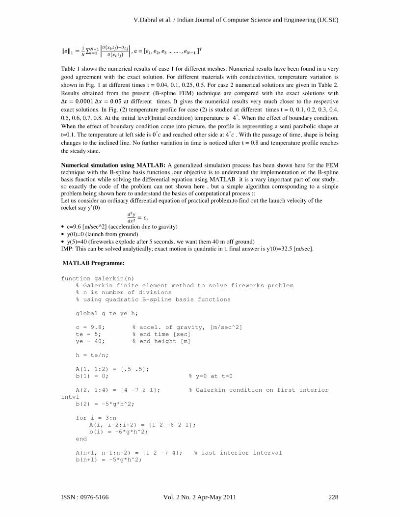
Numerical simulation using MATLAB: A generalized simulation process has been shown here for the FEM technique with the B-spline basis functions ,our objective is to understand the implementation of the B-spline basis function while solving the differential equation using MATLAB it is a vary important part of our study , so exactly the code of the problem can not shown here , but a simple algorithm corresponding to a simple problem being shown here to understand the basics of computational process :: Let us consider an ordinary differential equation of practical problem,to find out the launch velocity of the rocket say y’(0)

a?a? = ,

• c=9.6 [m/sec^2] (acceleration due to gravity) • y(0)=0 (launch from ground) • y(5)=40 (fireworks explode after 5 seconds, we want them 40 m off ground) IMP: This can be solved analytically; exact motion is quadratic in t, final answer is y'(0)=32.5 [m/sec]. MATLAB Programme:

function galerkin(n)

% Galerkin finite element method to solve fireworks problem

% n is number of divisions

% using quadratic B-spline basis functions

global g te ye h;

c = 9.8; % accel. of gravity, [m/sec^2]

te = 5; % end time [sec]

ye = 40; % end height [m]

h = te/n;

A(1, 1:2) = [.5 .5];

b(1) = 0; % y=0 at t=0

A(2, 1:4) = [4 -7 2 1]; % Galerkin condition on first interior

intvl

b(2) = -5*g*h^2;

for i = 3:n

A(i, i-2:i+2) = [1 2 -6 2 1];

b(i) = -6*g*h^2;

end

A(n+1, n-1:n+2) = [1 2 -7 4]; % last interior interval

b(n+1) = -5*g*h^2;



A(n+2, n+1:n+2) = [.5 .5];

b(n+2) = ye; % y=ye at t=te

b = b'; % make b into a column vector

u = A\b;

A

b'

u'

(u(2)-u(1))/h % initial velocity

% plot(-h/2:h:te+h/2, u, 'g'); % plot the coefficients

tv = 0:h/8:te; % supersample the parabolas

yv = [];

for t = tv

i = floor(t/h)+2;

if i==n+2

i = n+1;

end

x = t/h-i+1.5;

y = u(i-1)*.5*(x-.5)^2 + u(i)*(.75-x^2) + u(i+1)*.5*(x+.5)^2;

yv = [yv y];

end

% compute joints between elements

tk = (0:h:te)';

yk = .5*(u(1:n+1)+u(2:n+2));

hold off;

set(gca, 'FontSize', 16); % for tick marks

plot(tv,yv,'b', tk,yk,'bo', 'LineWidth',2);

xlabel('t', 'FontSize',20);

ylabel('y', 'FontSize',20);

axis([0 5 0 60]);

title('Galerkin Finite Element Method', 'FontSize',20);

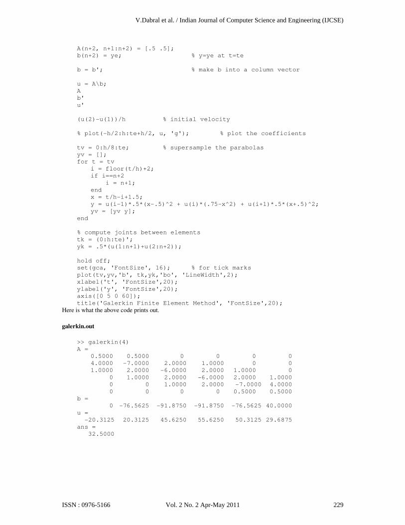
Here is what the above code prints out.

galerkin.out

>> galerkin(4)

A =

0.5000 0.5000 0 0 0 0

4.0000 -7.0000 2.0000 1.0000 0 0

1.0000 2.0000 -6.0000 2.0000 1.0000 0

0 1.0000 2.0000 -6.0000 2.0000 1.0000

0 0 1.0000 2.0000 -7.0000 4.0000

0 0 0 0 0.5000 0.5000

b =

0 -76.5625 -91.8750 -91.8750 -76.5625 40.0000

u =

-20.3125 20.3125 45.6250 55.6250 50.3125 29.6875

ans =

32.5000



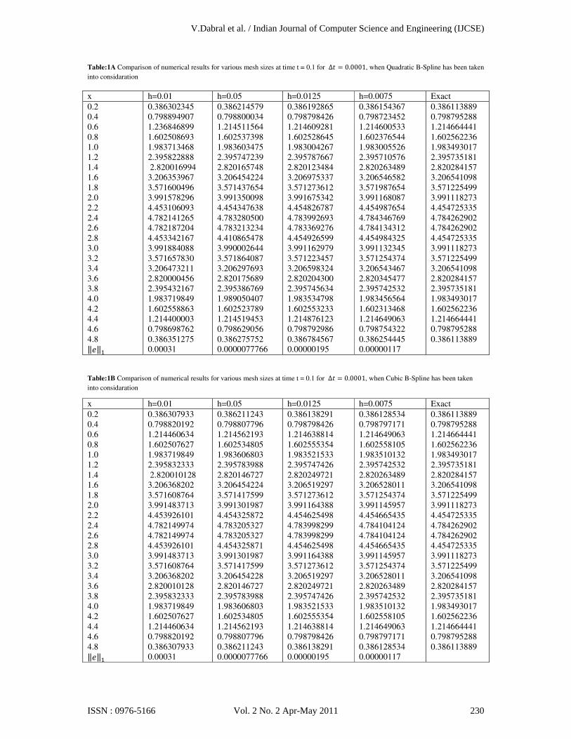
Table:1A Comparison of numerical results for various mesh sizes at time t = 0.1 for ∆ = 0.0001, when Quadratic B-Spline has been taken

into considaration

x h=0.01 h=0.05 h=0.0125 h=0.0075 Exact 0.2 0.4 0.6 0.8 1.0 1.2 1.4 1.6 1.8 2.0 2.2 2.4 2.6 2.8 3.0 3.2 3.4 3.6 3.8 4.0 4.2 4.4 4.6 4.8 ‖,‖

0.386302345 0.798894907 1.236846899 1.602508693 1.983713468 2.395822888 2.820016994 3.206353967 3.571600496 3.991578296 4.453106093 4.782141265 4.782187204 4.453342167 3.991884088 3.571657830 3.206473211 2.820000456 2.395432167 1.983719849 1.602558863 1.214400003 0.798698762 0.386351275 0.00031

0.386214579 0.798800034 1.214511564 1.602537398 1.983603475 2.395747239 2.820165748 3.206454224 3.571437654 3.991350098 4.454347638 4.783280500 4.783213234 4.410865478 3.990002644 3.571864087 3.206297693 2.820175689 2.395386769 1.989050407 1.602523789 1.214519453 0.798629056 0.386275752 0.0000077766

0.386192865 0.798798426 1.214609281 1.602528645 1.983004267 2.395787667 2.820123484 3.206975337 3.571273612 3.991675342 4.454826787 4.783992693 4.783369276 4.454926599 3.991162979 3.571223457 3.206598324 2.820204300 2.395745634 1.983534798 1.602553233 1.214876123 0.798792986 0.386784567 0.00000195

0.386154367 0.798723452 1.214600533 1.602376544 1.983005526 2.395710576 2.820263489 3.206546582 3.571987654 3.991168087 4.454987654 4.784346769 4.784134312 4.454984325 3.991132345 3.571254374 3.206543467 2.820345477 2.395742532 1.983456564 1.602313468 1.214649063 0.798754322 0.386254445 0.00000117

0.386113889 0.798795288 1.214664441 1.602562236 1.983493017 2.395735181 2.820284157 3.206541098 3.571225499 3.991118273 4.454725335 4.784262902 4.784262902 4.454725335 3.991118273 3.571225499 3.206541098 2.820284157 2.395735181 1.983493017 1.602562236 1.214664441 0.798795288 0.386113889

Table:1B Comparison of numerical results for various mesh sizes at time t = 0.1 for ∆ = 0.0001, when Cubic B-Spline has been taken

into considaration

x h=0.01 h=0.05 h=0.0125 h=0.0075 Exact 0.2 0.4 0.6 0.8 1.0 1.2 1.4 1.6 1.8 2.0 2.2 2.4 2.6 2.8 3.0 3.2 3.4 3.6 3.8 4.0 4.2 4.4 4.6 4.8 ‖,‖

0.386307933 0.798820192 1.214460634 1.602507627 1.983719849 2.395832333 2.820010128 3.206368202 3.571608764 3.991483713 4.453926101 4.782149974 4.782149974 4.453926101 3.991483713 3.571608764 3.206368202 2.820010128 2.395832333 1.983719849 1.602507627 1.214460634 0.798820192 0.386307933 0.00031

0.386211243 0.798807796 1.214562193 1.602534805 1.983606803 2.395783988 2.820146727 3.206454224 3.571417599 3.991301987 4.454325872 4.783205327 4.783205327 4.454325871 3.991301987 3.571417599 3.206454228 2.820146727 2.395783988 1.983606803 1.602534805 1.214562193 0.798807796 0.386211243 0.0000077766

0.386138291 0.798798426 1.214638814 1.602555354 1.983521533 2.395747426 2.820249721 3.206519297 3.571273612 3.991164388 4.454625498 4.783998299 4.783998299 4.454625498 3.991164388 3.571273612 3.206519297 2.820249721 2.395747426 1.983521533 1.602555354 1.214638814 0.798798426 0.386138291 0.00000195

0.386128534 0.798797171 1.214649063 1.602558105 1.983510132 2.395742532 2.820263489 3.206528011 3.571254374 3.991145957 4.454665435 4.784104124 4.784104124 4.454665435 3.991145957 3.571254374 3.206528011 2.820263489 2.395742532 1.983510132 1.602558105 1.214649063 0.798797171 0.386128534 0.00000117

0.386113889 0.798795288 1.214664441 1.602562236 1.983493017 2.395735181 2.820284157 3.206541098 3.571225499 3.991118273 4.454725335 4.784262902 4.784262902 4.454725335 3.991118273 3.571225499 3.206541098 2.820284157 2.395735181 1.983493017 1.602562236 1.214664441 0.798795288 0.386113889



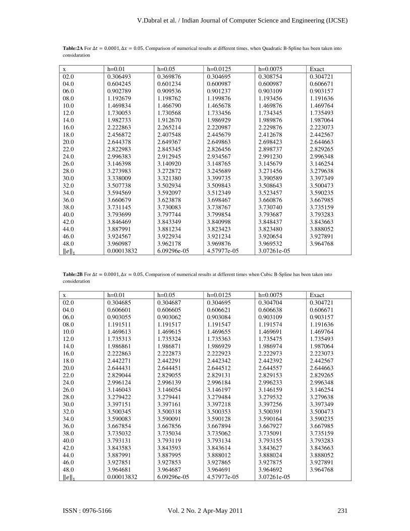
Table:2A For ∆ = 0.0001, ∆ = 0.05, Comparison of numerical results at different times, when Quadratic B-Spline has been taken into

considaration

x h=0.01 h=0.05 h=0.0125 h=0.0075 Exact 02.0 04.0 06.0 08.0 10.0 12.0 14.0 16.0 18.0 20.0 22.0 24.0 26.0 28.0 30.0 32.0 34.0 36.0 38.0 40.0 42.0 44.0 46.0 48.0 ‖,‖

0.306493 0.604245 0.902789 1.192679 1.469834 1.730053 1.982733 2.222863 2.456872 2.644378 2.822983 2.996383 3.146398 3.273983 3.338009 3.507738 3.594569 3.660679 3.731145 3.793699 3.846469 3.887991 3.924567 3.960987 0.00013832

0.369876 0.601234 0.909536 1.198762 1.466790 1.730568 1.912670 2.265214 2.407548 2.649367 2.845345 2.912945 3.140920 3.272872 3.321380 3.502934 3.592097 3.623878 3.730083 3.797744 3.843349 3.881234 3.922934 3.962178 6.09296e-05

0.304695 0.600987 0.901237 1.199876 1.465678 1.733456 1.986929 2.220987 2.445679 2.649863 2.826456 2.934567 3.148765 3.245689 3.399735 3.509843 3.512349 3.698467 3.738767 3.799854 3.840998 3.823423 3.921234 3.969876 4.57977e-05

0.308754 0.600987 0.903109 1.193456 1.469876 1.734345 1.989876 2.229876 2.412678 2.698423 2.898737 2.991230 3.145679 3.271456 3.390589 3.508643 3.523457 3.660876 3.730740 3.793687 3.848437 3.823480 3.920654 3.969532 3.07261e-05

0.304721 0.606671 0.903157 1.191636 1.469764 1.735493 1.987064 2.223073 2.442567 2.644663 2.829265 2.996348 3.146254 3.279638 3.397349 3.500473 3.590235 3.667985 3.735159 3.793283 3.843663 3.888052 3.927891 3.964768

Table:2B For ∆ = 0.0001,∆ = 0.05, Comparison of numerical results at different times when Cubic B-Spline has been taken into

consideration

x h=0.01 h=0.05 h=0.0125 h=0.0075 Exact 02.0 04.0 06.0 08.0 10.0 12.0 14.0 16.0 18.0 20.0 22.0 24.0 26.0 28.0 30.0 32.0 34.0 36.0 38.0 40.0 42.0 44.0 46.0 48.0 ‖,‖

0.304685 0.606601 0.903055 1.191511 1.469613 1.735313 1.986861 2.222863 2.442271 2.644431 2.829044 2.996124 3.146043 3.279422 3.397151 3.500345 3.590083 3.667854 3.735032 3.793131 3.843583 3.887991 3.927851 3.964681 0.00013832

0.304687 0.606605 0.903062 1.191517 1.469615 1.735324 1.986871 2.222873 2.442291 2.644451 2.829055 2.996139 3.146054 3.279441 3.397161 3.500318 3.590091 3.667856 3.735034 3.793119 3.843593 3.887995 3.927853 3.964687 6.09296e-05

0.304695 0.606621 0.903084 1.191547 1.469655 1.735363 1.986929 2.222923 2.442342 2.644512 2.829131 2.996184 3.146197 3.279484 3.397218 3.500353 3.590128 3.667894 3.735062 3.793134 3.843614 3.888012 3.927865 3.964691 4.57977e-05

0.304704 0.606638 0.903109 1.191574 1.469691 1.735475 1.986974 2.222973 2.442392 2.644557 2.829153 2.996233 3.146159 3.279532 3.397256 3.500391 3.590164 3.667927 3.735091 3.793155 3.843627 3.888024 3.927875 3.964692 3.07261e-05

0.304721 0.606671 0.903157 1.191636 1.469764 1.735493 1.987064 2.223073 2.442567 2.644663 2.829265 2.996348 3.146254 3.279638 3.397349 3.500473 3.590235 3.667985 3.735159 3.793283 3.843663 3.888052 3.927891 3.964768



Geometrical Interpretation:

The three dimensional geometrical Interpretation of the above phenomena has been shown in the Fig 1 to 5.for

different time level t=0.1,0.2 respectively for the distinguish coordinate domain, there is some duplication is

seemed at different time level.

Fig 1(A) and 1 (B)

Figure 1.The geometrical Interpretation of Heat equation at different time level t=0.1 and 0.2 at 0<x<1

Fig 2(A) and 2 (B)


Fig 3(A) and 3 (B) Figure 3.The geometrical Interpretation of Heat equation at different time level t=0.1 and 0.2 at 0<x<3



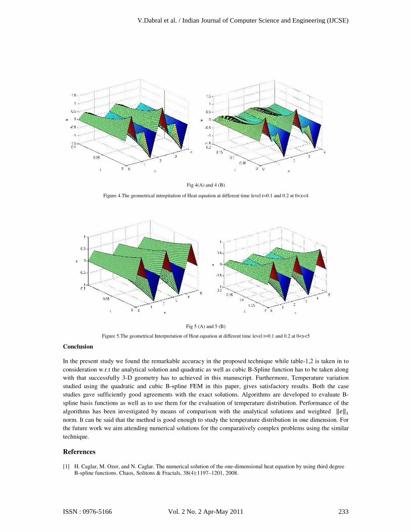
Fig 4(A) and 4 (B)

Figure 4.The geometrical intrepitation of Heat equation at different time level t=0.1 and 0.2 at 0<x<4

Fig 5 (A) and 5 (B)


Conclusion

In the present study we found the remarkable accuracy in the proposed technique while table-1,2 is taken in to

consideration w.r.t the analytical solution and quadratic as well as cubic B-Spline function has to be taken along

with that successfully 3-D geometry has to achieved in this manuscript. Furthermore, Temperature variation

studied using the quadratic and cubic B-spline FEM in this paper, gives satisfactory results. Both the case

studies gave sufficiently good agreements with the exact solutions. Algorithms are developed to evaluate B-

spline basis functions as well as to use them for the evaluation of temperature distribution. Performance of the

algorithms has been investigated by means of comparison with the analytical solutions and weighted ‖,‖

norm. It can be said that the method is good enough to study the temperature distribution in one dimension. For

the future work we aim attending numerical solutions for the comparatively complex problems using the similar

technique.

References

[1] H. Caglar, M. Ozer, and N. Caglar. The numerical solution of the one-dimensional heat equation by using third degree B-spline functions. Chaos, Solitons & Fractals, 38(4):1197–1201, 2008.



[2] A. Mohebbi and M. Dehghan. High-order compact solution of the one- dimensional heat and advection-diffusion equations. Applied Mathematical Modelling, In Press, Corrected Proof, 2010.

[3] I. Dag, D. Irk, and B. Saka. A numerical solution of the Burgers’ equation using cubic B-splines. Applied Mathematics and Computation, 163(1):199–211, 2005.

[4] M. Dehghan. A finite difference method for a non-local boundary value problem for two-dimensional heat equation. Applied Mathematics and Computation, 112(1):133–142, 2000.

[5] A. Gorguis and W. K. Benny Chan. Heat equation and its comparative solutions. Computers & Mathematics with Applications, 55(12):2973–2980, 2008.

[6] X. L. Han and S. J. Liu. An extension of the cubic uniform B-spline curves. Journal of Computer Aided Design and Computer Graphics, 15(5):576–578, 2003 (in chinese).

[7] M. Kumar and Y. Gupta. Methods for solving singular boundary value problems using splines: a review. Journal of Applied Mathematics and Computing, 32(1):265–278, 2010.

[8] H. W. Sun and J. Zhang. A high-order compact boundary value method for solving one-dimensional heat equations. Numerical Methods for Partial Differential Equations, 19(6):846–857, 2003.

[9] M. Tatari and M. Dehghan. A method for solving partial differential equations via radial basis functions: Application to the heat equation. Engineering Analysis with Boundary Elements, 34(3):206–212, 2010.

[10] G. Xu and G. Z. Wang. Extended cubic uniform B-spline and α-B-spline. Acta Automat. Sinica, 34(8):980–983, 2008. [11] C.I.Byrnes, D. Gilliam, V. Shubov and Z.Xu. Steady state response to Burgers’ equation with varying viscosity,

Progress in Systems and control: Computation and Control IV, (K.L.Bowers and J.Lund, eds.). Boston: Birkhauser, 1995, 75-98.

[12] A.Jameson. Airfoils admitting non-unique solutions of the Euler Equations, AIAA 22nd Fluid Dynamics, Plasmadynamics & Lasers Conference, Honolulu, June, 1991.

[13] Day, W.A.: Extension of a property of the heat equation to linear thermoelasticity and other theories, Quart. Appl. Math. 40, 319–330 (1982).

[14] Day, W.A.: A decreasing property of solutions of parabolic equations with applications to thermoelasticity, Quart. Appl. Math. 41, 468–475 (1983).

[15] Ekolin, G.: Finite difference methods for a nonlocal boundary value problem for the heat equation, BIT 31, 245–261 (1991).

[16] Liu, Y.: Numerical solution of the heat equation with nonlocal boundary conditions, J. Comput. Appl. Math. 110, 115–127 (1999).

[17] Jeffery Cooper. Introductin to Partial Differential Equations with Matlab. Birkhauser, Boston, 1998. [18] William F. Ames. Numerical Methods for Partial Differential Equations. Academic Press, Inc., Boston, third edition,

1992. [19] Clive A.J. Fletcher. Computational Techniquess for Fluid Dynamics. Springer-Verlag, Berlin, 1988. [20] K.W. Morton and D.F. Mayers. Numerical Solution of Partial Differential Equations: An Introduction. Cambridge

University Press, Cambridge, England, 1994. [21] Gene Golub and James M. Ortega. Scientific Computing: An Introduction with Parallel Computing. Academic Press,

Inc., Boston, 1993. [22] Joe D. Hoffman. Numerical Methods for Engineers and Scientists. McGraw-Hill, New York, 1992. [23] R. L. Burden and J. D. Faires. Numerical Analysis. Brooks/Cole Publishing Co., New York, sixth edition, 1997. [24] Eugene Isaacson and Herbert Bishop Keller. Analysis of Numerical Methods. Dover, New York, 1994. [25] Erwin Kreyszig. Advanced Engineering Mathematics. Wiley, New York, seventh edition, 1993. [26] I.J.Marwah, M.G.Chopra, Transient Heat Transfer in a slab with Heat Generation, Def. Sci J, 32(2)(1982), 143-149 [27] Elimoel A.Elias, Rogerio Cichota, Hugo H.Torriani and Quirijn De Jong van Lier, Analytical Soil-Temperature Model:

Correction for Temporal Variation of Daily Amplitude, Soil Sci.Soc.Am.J.68(2004), 784-788. [28] F.de Monte, Transient heat conduction in one-dimensional composite slab: A 'natural' analytic approach, International

Journal of Heat and Mass Transfer, 43 (2000), 3607-3619. [29] X Lu, P Tervola and M Viljanen, An e±cient analytical solution to the transient heat conduction in one dimensional

hollow composite cylinder, J. Phys. A. Math. Gen. 38(2005), 10145-10155. [30] J.H.Ahlberg, E.N.Nilson, J.L.Walsh, The Theory of Splines and their Applications, Acadamic Press, New York, (1967). [31] Klaus HÄolling, Finite Element Method with B-splines, SIAM, Philadelphia, (2003). [32] Masashi Kashiwagi, A B-spline Galerkin scheme for calculating the hydroelastic response of a very large roating

structure in waves, Journal of Marine Science and Technology, 3 (1998), 37-49. [33] Hartmut Prautzsch, A round trip to B-spline via de Casteljau, ACM Transactions on Graphics(TOG), 8(3) (1989), 243-

254. [34] A.R.Bahadir, Application of cubic B-spline finite element technique to the thermistor problem, Applied Mathematics

and Computation, 149 (2004), 379-387. [35] Liang Xuebiao, The B-spline finite elemenet method applied to axisymmetrical and nonlinear field problems, IEEE

Transactions on Magnetic, 24(1) (1988), 27-30 [36] Ni Guangzheng, Xu Xiaoming, Jian Baidun, B-spline Finite Element Method for Eddy Current field analysis, IEEE

Transactions on Magnetic, 26(2) (1990), 723- 726 [37] C.de Boor, A Practicle guide to splines, Applied Mathematical Sciences, Springer-Verlag, (2001) [38] Carl de Boor, On Calculating with B-splines, Journal of Approximation Theory, 6 (1972), 50-62. [39] L.F.Yang, The Spline Matrix Method, J. Guangxi Univ. 18(2)(1994), 61-65. [40] Z.Zong,K.Y.Lam, Estimation of complicated distributions using B-spline functions, Struct. Safety, 20(1998), 341-355. [41] Y.K.Cheung, S.C.Fan, C.Q.Wu, Spline finite strip in structural analysis, Proceedings of Intrnational Conference on

Finite Element Method, (1982), 704-709.



[42] Thomas A.Grandine, The Extensive use of Splines at Boeing, SIAM News,38(4)(2005) [43] Qiu Wu, Chandrajit L. Bajaj B-spline Representation for Volume Reconstruction, [44] P.M.Prenter, Splines and Variational Methods, Wiley, New York, (1975) [45] Carl de Boor, On Calculating with B-splines, Journal of Approximation Theory,6, (1972), 50-62. [46] J. Descloux, On the Numerical Integration of the Heat Equation, Numer. Math. 15 (1970), 371-381. [47] John C. Strikwerda, Finite difference schemes and partial differential equations, SIAM, (2004) [48] C.de Boor, A Practicle guide to splines, Applied Mathematical Sciences, Springer-Verlag, (2001) [49] Carl de Boor, On Calculating with B-splines, Journal of Approximation Theory, 6 (1972), 50-62. [50] L.F.Yang, The Spline Matrix Method, J. Guangxi Univ. 18(2)(1994), 61-65. [51] Z.Zong,K.Y.Lam, Estimation of complicated distributions using B-spline functions, Struct. Safety, 20(1998), 341-355.



numerical simulation of one dimensional heat equation: · pdf filenumerical simulation of one...

Documents