numerical simulation of morphogenetic … simulation of morphogenetic movements in ... numerical...
TRANSCRIPT

HAL Id: tel-00429691https://tel.archives-ouvertes.fr/tel-00429691v1
Submitted on 4 Nov 2009 (v1), last revised 4 Feb 2010 (v2)
HAL is a multi-disciplinary open accessarchive for the deposit and dissemination of sci-entific research documents, whether they are pub-lished or not. The documents may come fromteaching and research institutions in France orabroad, or from public or private research centers.
L’archive ouverte pluridisciplinaire HAL, estdestinée au dépôt et à la diffusion de documentsscientifiques de niveau recherche, publiés ou non,émanant des établissements d’enseignement et derecherche français ou étrangers, des laboratoirespublics ou privés.
Numerical simulation of morphogenetic movements inDrosophila embryo
Rachele Allena
To cite this version:Rachele Allena. Numerical simulation of morphogenetic movements in Drosophila embryo. Mechanics[physics.med-ph]. Ecole Centrale Paris, 2009. English. <tel-00429691v1>
Numerical simulation of morphogeneticmovements in Drosophila embryo
THESE
presentee et soutenue publiquement le 16/09/2009
pour l’obtention du
Doctorat de l’Ecole Centrale Paris
(specialite mecanique)
par
Rachele Allena
sous la direction de D. Aubry
Composition du Jury
President : D. Barthes-Biesel (UTC - Genie Biologique)
Rapporteurs : J. Munoz (Universitat Politecnica de Catalunya)P. Tracqui (Equipe DynaCell, Laboratoire TIMC)
Examinateurs : E. Farge (Institut Curie)A. Mouronval (Ecole Centrale Paris)
Laboratoire de Mecanique des Sols, Structures et Materiaux - CNRS U.M.R. 8579 - 2007-03


asap fslPhD
i

ii

Aknowledgements
In this section of the work remerciements obligent.First of all: no jury, no thesis. Therefore I would like to thank all the members
of the committee not only for their presence at my defense, but also and especiallyfor the time they have spent reading my manuscript.
Particular thank you to Emmanuel Farge and his passion for the DrosophilaMelanogaster, which has made possible this work. Even if sometimes it seemed tome very hard to catch your biological-physical vocabulary, as an engineer I havebeen pleased to work with you.
Thanks to Emmanuel Beaurepaire, Anne-Sophie Mouronval and Jose Munoz forthe interesting and helpful discussions.
I, me and myself say un enorme grazie to Denis Aubry: it has been amazing toshare with you my thoughts, even the silly ones!
Special thanks to Amelie, Elsa, Ghizlane and Sofia the best co-bureau ever...youare the best cadeau of MSSMat!
Finally to [email protected] and to all those people with whom I have laughed,cried, kidded around and many others during these last three years: grazie, graziedi cuore!
iii

iv

Motivation
Ourselves and all the endless forms we can observe around us are just the finalresult of a series of complex and still enigmatic processes that regulate nature. It isastonishing to discover little by little that we are part of an immense scheme whereeach single component knows exactly where to go, what to do and when and howto do it. Still more fascinating is to find out that the smallest parts of this system,at first sight the simplest ones, are instead the most organised and fundamental forthe success of the global plan. Cells can for sure be included in this category.
A cell is like a ”social being”: alone, even if extremely intelligent, it can notcompletely express itself, but together with other cells it can do unbelievable things.They are able to divide, proliferate, migrate and many others, but more importantlythey strongly co-operate to give rise to amazing 3D organisms. From the beginningof the embryogenesis therefore, everything is perfectly synchronized and the slightestimperfection may compromise the final result.
Since ever biologists have observed and studied intriguing developmental phases,trying to unveil the cryptic process by which an embryo is transformed in a livingorganism. Then mechanics may be very helpful in deciphering part of the wholeproblem. Each modification of the embryonic structure is actually driven by forcesgenerated within the cells that properly react and respond so that the global architec-ture changes, but the embryo can progressively perform more specialised functions.
The strong connection between mechanics and genetics has been studied for along time, showing how genes control and influence the occurrence of many morpho-genetic movements during embryogenesis. Only recently the inverse process has beendetected; it seems in fact that some mechanical forces might induce the expressionof specific genes, elsewhere than their usual area of action in the embryo.
Therefore two main conclusions can be drawn. First, embryonic cells, as similarlyas other types of cells in nature, are mechanosensible and able to adapt themselveswhen an external load is applied on them. Second, a mechanotransduction patternis present in the early embryo, so that a mechanical stimulus is transformed into achemical signal. If cells behaviour has been largely analyzed and explained throughmany and di!erent experiments on cultures, it is still not so clear how mechanicstransform a genetic information into a physical form. It would have been too ambi-tious to try to cover this gap, but at least with the present study we would like to
v

vi
o!er to the reader an exhaustive description of part of this complex process that isembryogenesis.
The huge advances made in numerical modeling allow today to couple togetherbiology and mechanics. Therefore it is possible not only to investigate those systemsthat so far appeared unapproachable, like the embryo, but also and more surprisinglyto discover that the minimal change of peculiar parameters may provide unexpectedand unordinary results. In this work we use computer simulations to reproduce someof the most interesting and studied events of Drosophila Melanogaster development.The main goal is to provide a useful support for biologists in order to confirm theirhypotheses resulted by experimental observations, but also and especially to pointout unexplored aspects so that new issues are suggested.

Thesis outline
The present thesis is developed through four principal chapters. The first one pro-vides a brief but rather exhaustive description of the context, with a global overviewon the complex process of the embryogenesis in Drosophila Melanogaster. We amplyfocus on the three morphogenetic movements that will be numerically simulated,with particular emphasis on both the mechanical and the biological aspects thatconstitute the main peculiarity of each event. Also we propose a short review on therelated previous works.
The second chapter supplies the abstract tools for the analysis of the wholeproblem and points out the hypotheses that, for sake of simplicity, have been made.The gradient decomposition method is presented together with some interestinginterpretations that better clarify the approach and put forward novel issues thathave to be considered. By the Principle of the Virtual Power, we are able to writethe mechanical equilibrium of the system which consists of the forces internal tothe embryo domain and of the boundary conditions, such as the yolk pressure andcontact with the vitelline membrane, that are essential for consistent results. Aspecial concern is attributed to the choice of the constitutive law of the mesodermthat, from a biological point of view, may appear too simplistic. Here a Saint-Venant material is used in contrast with the Hyperelastic models found in literature;therefore a comparison between the two is proposed together with the advantagesand the limitations of our study. Finally, we provide some simple examples thatvalidate our model and support the exploited method.
The third chapter can be divided into two parts. In the first one, by the paramet-rical description of the embryo geometry, we obtain the analytical formulations ofthe active deformation gradients for each morphogenetic movement according to theelementary forces introduced. Such expressions will be combined with the passivegradients in order to get the final deformation of the tissues. In the second part weinterpret the results for each simulation. In particular, we provide a parametricalanalysis for the simulation of the ventral furrow invagination, while for the germband extension a comparison with experimental data is done. Furthermore we havebeen able to estimate the e!ects induced by the local deformations within the tis-sues; specifically, we have evaluated the magnitude of the pressure forces and theshear stress that may develop at long distance in the embryo when the active forces
vii
viii
are applied in restraint regions. To conclude, we propose a collateral study on theinfluence of the global geometry of the embryo on the final results.
Given the consistence of the results for the individual simulations, we have de-cided to test the concurrent simulation of the events, by two or three of them. In thelast chapter, we show the results for a first essay for which we use the most intuitivemethod; it does not require in fact further manipulations of the analytical formu-lations previously obtained, but we simply couple together the active deformationgradients, following the chronological order of the movements. Although the methodworks well for the simulation of the two furrows, some drawbacks are detected whenwe introduce the germ band extension. Therefore we propose a new approach, morerigorous and appropriate, which allows to take into account some aspects so far putaside, but still significant for a realistic and complete reproduction of the di!erentphases of the Drosophila gastrulation.

Resume
Ce travail de recherche a eu comme objectif principal la conception d’un modelenumerique aux elements finis donnant une representation realiste des mouvementsde l’embryon de la Drosophila Melanogaster. Les simulations de trois mouvementsdurant la phase de gastrulation de l’embryon ont ete realisees soit individuelles soitsimultanees, ce qui jusqu’a present, n’a jamais ete propose, constituant ainsi unecontribution originale de cette etude.
La these est composee de quatre chapitres. Le premier fournit une breve maisassez complete description du contexte dans lequel ce travail se situe. Le proces-sus complexe de l’embryogenese chez la Drosophila Melanogaster est presente ense focalisant sur les trois mouvements morphogenetiques qui seront ensuite simulesnumeriquement: l’invagination du sillon ventral, la formation du sillon cephaliqueet l’extension de la bande germinale. Chaque evenement est decrit du point de vuebiologique et mecanique, ce qui permet donc de mettre en avant les aspects les plusinteressants des di!erents mouvements. Une revue des plus recents travaux est aussiproposee a fin de
Dans le deuxieme chapitre on presente les outils analytiques pour l’analyse duprobleme dans son integrite. Etant donnee la complexite du systeme biologique,plusieurs hypotheses ont ete introduites pour simplifier l’approche numerique util-isee. Seul le mesoderme est modelise comme un milieu continu dans un espacetridimensionel par un ellipsoıde epais regulier de 500µm de longueur. La methodede la decomposition du gradient de deformation, dont quelques interpretations al-ternatives sont presentees, permet de coupler les deformations passives et activessubies par chaque point materiel du milieu. L’equilibre mecanique est ecrit a partirdu Principe des Puissances Virtuelles: les forces internes du systeme sont donc prisesen compte avec les conditions aux limites. Dans notre cas particulier celles-ci sontfondamentales pour obtenir des configurations finales realistes et comprennent le con-tact entre le mesoderme et la membrane vitelline externe et le pression exercee par leyolk sur la surface interne du mesoderme. Les proprietes mecaniques des tissus em-bryonnaires ne sont pas faciles a determiner experimentalment. Une approximationa ete faite pour ce qui concerne la loi de comportement du mesoderme qui a ete mod-elise comme un materiau de Saint-Venant lineaire, elastique et isotrope. Notre choixetant en contraste avec le modele hyperelastique qu’on retrouve souvent en litera-
ix
x
ture, une comparaison entre les deux materiaux est proposee tout en considerant lesavantages et les limitations de notre demarche. La methode de la decomposition dugradient de deformation a ete auparavant testee sur des cas geometriquement tressimples dont la solution analytique peut etre facilement calculee et validee par lesresultats obtenus a partir des simulations numeriques.
Le troisieme chapitre peut etre divise en deux parties distinctes. Dans la pre-miere, grace a la description parametrique de l’ellipsoıde qui represente l’embryon,on calcule les expressions analytiques des positions intermediaires ou on voit appa-raıtre les deformations actives responsables de chaque mouvement morphogenetique.Les gradients de deformation active sont donc couples avec les gradients passifs pourobtenir la deformation finale. La deuxieme partie du chapitre concerne l’analyse desresultats pour les simulations individuelles des evenements. Pour la simulation del’invagination du sillon ventral une etude parametrique a ete conduite pour evaluerl’influence de certains parametres sur la configuration finale. Pour la simulation del’extension de la bande germinale les resultats ont ete compares avec les donnees ex-perimentales. En particulier on s’est interesse a l’analyse des contraintes mecaniques(les pressions et les contraintes de cisaillement) induites au niveau du pole anterieurou un chemin de mecanotransduction aurait lieu et conduirait a l’expression dutwist, un gene normalement exprime seulement dans la partie ventrale de l’embryon.Pour conclure, d’autres geometries que celle de l’ellipsoıde ont ete utilisees pour lessimulations de l’invagination du sillon ventral et de l’extension de la bande germi-nale. Ces nouvelles representations de l’embryon permettent de prendre en comptedeux aspects interessants: d’un cote l’arrondissement des deux poles, de l’autrel’aplatissement de la partie dorsal par rapport a la partie ventrale.
Le dernier chapitre du manuscrit introduit la simulation simultanee des troismouvements qui a ete mise en place pour deux raisons principales. Tout d’abord lefait que les evenements analyses se produisent l’un apres l’autre lors du developpe-ment de l’embryon. Deuxiemement, les resultats obtenus pour les simulations in-dividuelles sont tres encourageants et ont permis aussi de confirmer plusieurs hy-potheses avancees par les biologistes; d’ou l’interet de coupler les mouvements pourpermettre une vision encore plus realiste de cette phase importante de la gastrulationchez l’embryon de la Drosophila Melanogaster. Deux methodes di!erentes ont etetestees. La premiere, la plus intuitive et simple, permet de combiner les gradientsde deformation active de chaque mouvement et ne requiert pas de manipulationssupplementaires des equations precedemment trouvees, tout en prenant en comptele dephasage reel entre les evenements. Cette approche ne pose pas de problemesquand seulement les deux sillons sont couples, alors que l’introduction de l’extensionde la bande germinale donne lieu a quelque limitations. Une nouvelle demarche estdonc proposee, plus rigoureuse et precise, qui nous a permis de considerer certainsaspects importants pas encore developpes d’un point de vue theorique.

Contents
Contents xiii
List of Figures xvii
1 Introduction 11.1 Embryogenesis . . . . . . . . . . . . . . . . . . . . . . . . . . . . . . 1
1.1.1 General overview of insect embryogenesis . . . . . . . . . . . 21.2 Drosophila embryo . . . . . . . . . . . . . . . . . . . . . . . . . . . . 4
1.2.1 Stages of development . . . . . . . . . . . . . . . . . . . . . . 51.2.2 Invagination . . . . . . . . . . . . . . . . . . . . . . . . . . . . 91.2.3 Ventral furrow Invagination . . . . . . . . . . . . . . . . . . . 101.2.4 Cephalic furrow formation . . . . . . . . . . . . . . . . . . . . 221.2.5 Convergence-extension movements . . . . . . . . . . . . . . . 241.2.6 Cells rearrangement models . . . . . . . . . . . . . . . . . . . 281.2.7 Germ band extension . . . . . . . . . . . . . . . . . . . . . . 29
1.3 Conclusions . . . . . . . . . . . . . . . . . . . . . . . . . . . . . . . . 31
2 The kinematic model 352.1 Gradient decomposition method . . . . . . . . . . . . . . . . . . . . 362.2 The Principle of the Virtual Power . . . . . . . . . . . . . . . . . . . 432.3 The constitutive law of the mesoderm . . . . . . . . . . . . . . . . . 472.4 Pseudo-thermal interpretation of the gradient decomposition method 512.5 Interpretation in the case of a non uniform active zone . . . . . . . . 532.6 Validation of the model . . . . . . . . . . . . . . . . . . . . . . . . . 57
2.6.1 Deformation of a 2D beam . . . . . . . . . . . . . . . . . . . 582.6.2 Deformation of a 3D beam . . . . . . . . . . . . . . . . . . . 622.6.3 Radial and circular deformation of a circular cylinder section 642.6.4 Radial and circular deformation of a sphere . . . . . . . . . . 66
2.7 Required boundary conditions . . . . . . . . . . . . . . . . . . . . . . 722.7.1 Contact with the vitelline membrane . . . . . . . . . . . . . . 722.7.2 Internal yolk pressure . . . . . . . . . . . . . . . . . . . . . . 76
xi
xii Contents
2.8 Iterative scheme and finite elements approximation . . . . . . . . . . 802.9 Hints for a future stability analysis . . . . . . . . . . . . . . . . . . . 822.10 Conclusions . . . . . . . . . . . . . . . . . . . . . . . . . . . . . . . . 83
3 Morphogenetic movements in Drosophila embryo 873.1 Parametrical description of the embryo . . . . . . . . . . . . . . . . . 883.2 Ventral furrow invagination and cephalic furrow formation . . . . . . 913.3 Germ band extension . . . . . . . . . . . . . . . . . . . . . . . . . . . 973.4 Results . . . . . . . . . . . . . . . . . . . . . . . . . . . . . . . . . . . 1003.5 Ventral furrow invagination . . . . . . . . . . . . . . . . . . . . . . . 103
3.5.1 Influence of the size of the active deformation region . . . . . 1063.5.2 Influence of the dimensions of the material cells . . . . . . . . 1073.5.3 Influence of the apico-basal elongation . . . . . . . . . . . . . 108
3.6 Cephalic furrow formation . . . . . . . . . . . . . . . . . . . . . . . . 1133.7 Germ band extension . . . . . . . . . . . . . . . . . . . . . . . . . . . 1153.8 Hyperelastic model tested for GBE . . . . . . . . . . . . . . . . . . . 1193.9 Estimation of the induced forces through the embryo . . . . . . . . . 1203.10 Estimation of the induced shear stress through the embryo . . . . . 1243.11 Influence of the geometry on VFI and GBE . . . . . . . . . . . . . . 1253.12 Conclusions . . . . . . . . . . . . . . . . . . . . . . . . . . . . . . . . 131
4 Concurrent simulation of morphogenetic movements 1354.1 Lagrangian formulation . . . . . . . . . . . . . . . . . . . . . . . . . 1364.2 Updated Lagrangian formulation . . . . . . . . . . . . . . . . . . . . 145
4.2.1 Kinematic description . . . . . . . . . . . . . . . . . . . . . . 1454.2.2 The Principle of the Virtual Power and stress updated scheme 152
4.3 Conclusions . . . . . . . . . . . . . . . . . . . . . . . . . . . . . . . . 154
5 Conclusions and perspectives 157
A Large deformation theory 163A.1 The deformation gradient tensor . . . . . . . . . . . . . . . . . . . . 163A.2 Strain and deformation measures . . . . . . . . . . . . . . . . . . . . 166A.3 Large deformation stress measures . . . . . . . . . . . . . . . . . . . 167
B Mechanics of growing mass 171B.1 Surface growth . . . . . . . . . . . . . . . . . . . . . . . . . . . . . . 172B.2 Volumetric growth . . . . . . . . . . . . . . . . . . . . . . . . . . . . 173
C Special coordinate system 177C.1 Cylindrical polar coordinates . . . . . . . . . . . . . . . . . . . . . . 177C.2 Spherical polar coordinates . . . . . . . . . . . . . . . . . . . . . . . 179

Contents xiii
Bibliography 181

xiv Contents
List of Figures
1.1 Stages of embryogenesis . . . . . . . . . . . . . . . . . . . . . . . . . 61.2 Di!erent types of invagination . . . . . . . . . . . . . . . . . . . . . . 91.3 Hinge points during VFI . . . . . . . . . . . . . . . . . . . . . . . . . 111.4 Ventral furrow invagination . . . . . . . . . . . . . . . . . . . . . . . 121.5 Genes control on ventral furrow invagination . . . . . . . . . . . . . 131.6 Cell model by Odell . . . . . . . . . . . . . . . . . . . . . . . . . . . 151.7 Results by Odell . . . . . . . . . . . . . . . . . . . . . . . . . . . . . 171.8 The cortical model by Jacobson . . . . . . . . . . . . . . . . . . . . . 181.9 The shell model by Hardin and Cheng . . . . . . . . . . . . . . . . . 191.10 2D Finite Elements model by Munoz . . . . . . . . . . . . . . . . . . 221.11 3D Finite Elements model by Conte . . . . . . . . . . . . . . . . . . 231.12 Parametric study on Conte’s model . . . . . . . . . . . . . . . . . . . 241.13 Cephalic furrow . . . . . . . . . . . . . . . . . . . . . . . . . . . . . . 251.14 Cells rearrangement process . . . . . . . . . . . . . . . . . . . . . . . 271.15 Cells rearrangement model by Weliki . . . . . . . . . . . . . . . . . . 291.16 Cells rearrangement model by Jacobson . . . . . . . . . . . . . . . . 30
2.1 Gradient decomposition method . . . . . . . . . . . . . . . . . . . . 382.2 Constrained cell . . . . . . . . . . . . . . . . . . . . . . . . . . . . . . 392.3 Neighbour cells . . . . . . . . . . . . . . . . . . . . . . . . . . . . . . 402.4 Covariant base vectors . . . . . . . . . . . . . . . . . . . . . . . . . . 422.5 Series of 2D cellular domains . . . . . . . . . . . . . . . . . . . . . . 542.6 Heaviside function . . . . . . . . . . . . . . . . . . . . . . . . . . . . 562.7 2D beam geometry . . . . . . . . . . . . . . . . . . . . . . . . . . . . 592.8 2D beam longitudinal dilatation . . . . . . . . . . . . . . . . . . . . . 602.9 3D beam longitudinal dilatation . . . . . . . . . . . . . . . . . . . . . 682.10 2D cylindrical section geometry . . . . . . . . . . . . . . . . . . . . . 692.11 Radial dilatation of a cylindrical section . . . . . . . . . . . . . . . . 692.12 Circular dilatation of a cylindrical section . . . . . . . . . . . . . . . 702.13 Geometry of a sphere . . . . . . . . . . . . . . . . . . . . . . . . . . . 702.14 Radial dilatation of a sphere . . . . . . . . . . . . . . . . . . . . . . . 71
xv
xvi List of Figures
2.15 Circular dilatation of a sphere . . . . . . . . . . . . . . . . . . . . . . 712.16 Invagination and evagination of the mesoderm . . . . . . . . . . . . . 742.17 External contact during circular deformation of a sphere . . . . . . . 77
3.1 Cross-sectional view of the geometry of the embryo . . . . . . . . . . 893.2 Ventral furrow invagination . . . . . . . . . . . . . . . . . . . . . . . 923.3 Elementary cell deformations during VFI . . . . . . . . . . . . . . . 933.4 Periodic function for theta . . . . . . . . . . . . . . . . . . . . . . . . 943.5 Elementary cell deformations during CF formation . . . . . . . . . . 953.6 Elementary cell deformations during GBE . . . . . . . . . . . . . . . 983.7 Embryo geometry . . . . . . . . . . . . . . . . . . . . . . . . . . . . . 1013.8 Embryo mesh . . . . . . . . . . . . . . . . . . . . . . . . . . . . . . . 1033.9 Active deformation region for VFI . . . . . . . . . . . . . . . . . . . 1043.10 Successive phases of VFI . . . . . . . . . . . . . . . . . . . . . . . . . 1093.11 Incompatibility due to the active deformation . . . . . . . . . . . . . 1103.12 Variation of the active deformation region for VFI . . . . . . . . . . 1103.13 Influence of the size of the deformation region . . . . . . . . . . . . . 1113.14 Influence of the dimensions of the material cells . . . . . . . . . . . . 1113.15 Influence of the apico-basal deformation . . . . . . . . . . . . . . . . 1123.16 Active deformation region for CF . . . . . . . . . . . . . . . . . . . . 1143.17 Results for CF . . . . . . . . . . . . . . . . . . . . . . . . . . . . . . 1153.18 Active deformation region for the GBE . . . . . . . . . . . . . . . . . 1163.19 Results for the GBE simulation . . . . . . . . . . . . . . . . . . . . . 1173.20 Velocity field for the GBE . . . . . . . . . . . . . . . . . . . . . . . . 1183.21 Hyperelastic model for GBE . . . . . . . . . . . . . . . . . . . . . . . 1193.22 Volume variation for VFI simulation . . . . . . . . . . . . . . . . . . 1233.23 Volume variation for GBE simulation . . . . . . . . . . . . . . . . . . 1243.24 Di!erent geometries tested for VFI and GBE . . . . . . . . . . . . . 1273.25 Di!erent geometries tested for VFI: frontal sections . . . . . . . . . . 1283.26 Di!erent geometries tested for VFI: cross sections . . . . . . . . . . . 1293.27 Di!erent geometries tested for GBE . . . . . . . . . . . . . . . . . . 1303.28 4th geometry . . . . . . . . . . . . . . . . . . . . . . . . . . . . . . . 1313.29 5th geometry . . . . . . . . . . . . . . . . . . . . . . . . . . . . . . . 131
4.1 Active regions of deformation for the concurrent simulation of VFIand CF . . . . . . . . . . . . . . . . . . . . . . . . . . . . . . . . . . 138
4.2 Time history of the concurrent simulation for VFI and CF . . . . . . 1394.3 Concurrent simulation of the two furrows . . . . . . . . . . . . . . . 1414.4 Time history of the concurrent simulation of the three morphogenetic
movements . . . . . . . . . . . . . . . . . . . . . . . . . . . . . . . . 1424.5 Active regions of deformation for the concurrent simulation of VFI,
CF and GBE . . . . . . . . . . . . . . . . . . . . . . . . . . . . . . . 143

List of Figures xvii
4.6 Concurrent simulation of the three morphogenetic movements . . . . 1444.7 Updated Lagrangian method . . . . . . . . . . . . . . . . . . . . . . 1474.8 Convergence-extension movement on an apically constricted cell . . . 1494.9 Cross-sectional view of the deformed geometry of the embryo . . . . 1504.10 Successive phases of the updated concurrent simulation . . . . . . . 153
A.1 Undeformed and deformed configurations . . . . . . . . . . . . . . . 164A.2 Di!erential area element before and after deformation . . . . . . . . 166
B.1 Surface growth . . . . . . . . . . . . . . . . . . . . . . . . . . . . . . 173B.2 Volumetric growth . . . . . . . . . . . . . . . . . . . . . . . . . . . . 175
C.1 Cylindrical polar coordinates . . . . . . . . . . . . . . . . . . . . . . 178C.2 Spherical polar coordinates . . . . . . . . . . . . . . . . . . . . . . . 179

xviii List of Figures
Chapter 1
Introduction
This chapter can be divided into two parts. The first one provides a general overviewof the embryogenesis so that the reader may get familiar with the embryo vocabulary(Sec. 1.1). The di!erent phases of Drosophila embryo development are describedwith particular emphasis on the biological aspects of the process (Sec. 1.2). Inthe second part instead, we focus on the three morphogenetic movements that arenumerically simulated later; ventral furrow invagination (Sec. 1.2.3), cephalic furrowformation (Sec. 1.2.4) and germ band extension (Sec. 1.2.7). We first describe thedi!erent class movements to which the specific events previously mentioned belong(Sec. 1.2.2, 1.2.5); then we switch to a more detailed analysis of each event pointingout the mechanics of the problem, without omitting the influence exerted by specificgenes on them. Aware that mechanical modeling plays an important role in theunderstanding of the di!erent phases of embryogenesis, we also present a review ofthe works we have found in literature. Particularly, Sec. 1.2.3.1 is dedicated toventral furrow invagination while Sec. 1.2.6 to convergence-extension movements.
1.1 Embryogenesis
Embryogenesis - how the tissues and organs of the developing embryo take theirforms - is a very complex process which has traditionally been explained in termsof genes, hormones and chemical gradients. Usually it begins once the egg has beenfertilized and it involves multiplication of cells (by mitosis) and their subsequentgrowth, movement and di!erentiation into all the tissues and organs of a livinginsect. Given the remarkable similarity in genes responsible for organizing the fun-damental body plan in vertebrates and invertebrates, in the last few years the fieldof insect embryology has played a significant role in the understanding of develop-mental processes of humans and other vertebrate organisms. Even if much of insectembryology still remains mysterious, there has been a notable progress in knowledgethanks to new methods in molecular biology and genetic engineering. Particularly, it
1

2 Chapter 1. Introduction
has recently been shown that biomechanics plays an important role in the formation,repair and function of bones, organs and arteries (Holzapfel [2000], Taber [2004]),but it plays an equally important role at the scale of cells and the scale of the em-bryo. For this reason, developmental processes have been largely studied in terms ofmechanics and physics, although still little is known on how a genetic informationcan be translated via mechanics (i.e. forces and movements) into a physical form.
Insect embryogenesis can be described through a precise series of common stages;in the next section we provide a general overview (also refer to LeMoigne and Foucrier[2004] and to Forgacs and Newman [2006]) of the processes involved. Later on we willfocus on Drosophila Melanogaster development, which is the object of the presentstudy; the analysis of three specific morphogenetic movements will point out thestrong connections between biology and mechanics. Actually, it has been recentlyshown that not only genetics may control mechanical forces and deformations of theembryo, as it has been observed and demonstrated so far, but also the vice versacan occur and therefore mechanotransduction and mechanosensibility paths may beanalyzed and taken into account (Brouzes and Farge [2004], Farge [2003]).
1.1.1 General overview of insect embryogenesis
An insect’s egg is much too large and full of yolk to simply divide in half like a humanegg during its initial stages of development; for this reason, insects ”clone” the zygotenucleus by mitosis without cytokinesis through 12-13 division cycles to yield about5000 daughter nuclei. This process of nuclear division is known as superficial cleav-age; once formed, the cleavage nuclei migrate through the yolk toward the perimeterof the egg and they subside in the band of periplasm where they construct the mem-branes to create individual cells. The final result of the cleavage is the blastoderm,a one-cell-thick layer of cells surrounding the yolk. The first cleavage nuclei to reachthe vicinity of the oosome are ”reserved” for future reproductive purposes, thus theydo not travel to the periplasm and do not form any part of the blastoderm. Instead,they stop dividing and form germ cells that remain segregated throughout much ofembryogenesis: these cells will eventually migrate into the developing gonads andonly when the adult insect finally reaches sexual maturity they will begin by meiosisto form gametes of the next generation. This means that germ cells never grow ordivide during embryogenesis, therefore DNA is conserved from the very beginningof the development. The principal reason of this strategy is to minimize the risk ofan error in replication that would accidently be passed on to the next generation.
The blastoderm cells start enlarging and multiply on one side of the egg and thisregion, called germ band or ventral plate, is exactly where the embryo’s body willdevelop. The rest of the cells become part of a membrane, the serosa, that formsthe yolk sac; these cells grow around the germ band, enclosing the embryo in anamniotic membrane.
At this stage of embryogenesis, when the embryo is composed by a single layer of

1.2 Drosophila embryo 3
cells, a specific group of control genes, the so called homeotic selector genes, becomeactive. These genes, by proteins with special active site, bind with the DNA andinteract with particular locations in the genome where they activate or inhibit theexpression of other genes. Practically, each selector gene, within a restricted domainof cells according to their location in the germ band, controls the expression of othergenes that produce hormone-like ”organizer” chemicals, cell-surface receptors andstructural elements. Also the selector genes guide the development of individual cellsand channel them into di!erent functions. Such process is called di!erentiation andcontinues until the fundamental body plan is mapped out; firstly into general regionsalong the anterior-posterior axis, secondly into individual segments and finally intospecialized structures or appendages.
When the germ band starts enlarging, it is possible to observe it lengtheningand folding so that its final shape corresponds to a layer of cells on the outside, theectoderm, and another one on the inside, the mesoderm. Once the lateral edgesof the germ band fuse along the dorsal midline of the embryo, the dorsal closureoccurs. At this stage, ectodermal cells grow and di!erentiate forming the epidermis,the brain, the nervous system and most of the insect’s tracheal system. Furthermore,the ectoderm folds inward at the front (foregut) and rear (hindgut) regions of thedigestive system. On the other hand, mesodermal cells di!erentiate to form otherinternal structures such as muscles, glands, heart, blood and reproductive organs.The midgut generates from a third layer, the endoderm, which arises near the foreand hindgut invaginations and eventually fuse with them to complete the alimentarycanal.
During early development, the embryo looks most like a worm and only laterfirst segments become visible near the anterior end, to move through the thorax andthe abdomen. Generally, the rate of embryonic development is influenced by thetemperature and by the specific characteristics of species. The entire process endswhen the yolk’s contents have been completely consumed so that the insect is fullyformed and ready to hatch the egg. The eclosion may take place by a chewing ofthe insect through the egg’s chorion or simply the insect can swell in size until theegg shell cracks along a predetermined line of weakness. Contrary to the generalthought, the larva does not end its development with the hatching process, but itwill continue to develop and mature.
1.2 Drosophila embryo
Drosophila melanogaster is a two-winged insect that belongs to the species of theflies. The species is usually known as the common fruit fly and it is the most studiedorganism in biological research, particularly in genetics and developmental biology.There are several reasons:
4 Chapter 1. Introduction
• it is small and easy to grow in laboratory;
• it has a short generation time (about two weeks) so several generations can bestudied within few weeks;
• it presents high fecundity;
• it has only four pairs of chromosomes;
• genetic transformation techniques have been available since 1987;
• its compact genome was sequenced and first published in 2000 (Adams et al.[2000]).
Drosophila melanogaster has also some similarities with the human embryo; infact 75% of known human disease genes have a recognizable match in the geneticcode of fruit flies and 50% of fly protein sequences have mammalian analogues (Reiter[2001]). Embryogenesis in Drosophila has been extensively studied since the smallsize and short generation makes it ideal for genetic studies. It is also unique amongmodel organisms in which cleavage occurs in a synctium.
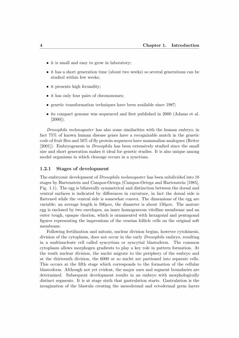
1.2.1 Stages of development
The embryonic development of Drosophila melanogaster has been subdivided into 18stages by Hartenstein and Campos-Ortega (Campos-Ortega and Hartenstein [1985],Fig. 1.1). The egg is bilaterally symmetrical and distinction between the dorsal andventral surfaces is indicated by di!erences in curvature, in fact the dorsal side isflattened while the ventral side is somewhat convex. The dimensions of the egg arevariable; an average length is 500µm, the diameter is about 150µm. The matureegg is enclosed by two envelopes, an inner homogeneous vitelline membrane and anouter tough, opaque chorion, which is ornamented with hexagonal and pentagonalfigures representing the impressions of the ovarian follicle cells on the original softmembrane.
Following fertilization and mitosis, nuclear division begins, however cytokinesis,division of the cytoplasm, does not occur in the early Drosophila embryo, resultingin a multinucleate cell called syncytium or syncytial blastoderm. The commoncytoplasm allows morphogen gradients to play a key role in pattern formation. Atthe tenth nuclear division, the nuclei migrate to the periphery of the embryo andat the thirteenth division, the 6000 or so nuclei are partioned into separate cells.This occurs at the fifth stage which corresponds to the formation of the cellularblastoderm. Although not yet evident, the major axes and segment boundaries aredetermined. Subsequent development results in an embryo with morphologicallydistinct segments. It is at stage sixth that gastrulation starts. Gastrulation is theinvagination of the blastula creating the mesodermal and ectodermal germ layers

1.2 Drosophila embryo 5
Figure 1.1: Successive phases of Drosophila embryo development(http://biology.kenyon.edu).
and usually is a very complex phase of the development of vertebrates; in the flyit is overwhelming. There is not just a single site for cell invagination, but takentogether, one finds approximatively ten morphogenetic movements, three of whichcan be considered gastrulation proper and seven more that should be analyzed inorder to understand Drosophila embryogenesis as a whole. Of the three events oneis involved in mesoderm formation, the ventral furrow invagination, and two othersinvolve endoderm formation, both anterior and posterior midgut invagination (Costaet al. [1993]). Seven other events resembling gastrulation are listed below:
• formation of the cephalic furrow;
• formation of dorsal transverse folds;
• germ band extension;
• germ band retraction;
• segmentation;
• dorsal closure;
• head involution.

6 Chapter 1. Introduction
It has to be known that there are other programs of cell movement, includingtrachea formation, imaginal disc development and segregation of neuroblasts fromthe neuroectoderm. The initial structuring for most of these events can be tracedback to the four maternal systems which establish polarity in the egg and, as aconsequence, in the zygote. Thus these events are related to segmentation patternsbuilt early in development. Ventral furrow formation and dorsal closure have theirorigin in the dorsal-ventral system; the other eight events originate with the anteriorand the posterior group of maternal genes, that are responsible for anterior-posteriorpolarity.
Gastrulation begins three hours after fertilization; by this time there have beenthirteen mitotic cycles. Prior to the tenth cycle, the dividing nuclei lie in the interiorof the egg, but move out toward the surface, going through four more division cyclesat the periphery until cellularization occurs (Foe et al. [1993]). Immediately aftercellularization, a process taking less than a hour to complete, the ventral furrow,which marks the beginning of gastrulation, begins to form.
During Drosophila gastrulation it is possible to observe two major invaginations:the ventral furrow and the posterior midgut, that internalize mesodermal and pos-terior endodermal precursor cells respectively (Sweeton et al. [1991]). Cells thatinternalize by the ventral furrow invagination will give rise to the mesoderm andabout eight minutes after the ventral furrow begins to form, the posterior midgutinvagination starts at the posterior pole with internalization of cells rising the endo-derm.
As underlined above, in Drosophila embryo several mechanical movements occur.Even if they take place at di!erent stages of development and at di!erent regionsof the embryo, some of them are thought to be driven by the same coordinatedchanges in shape of individual cells at the site of active movement, which generateglobal changes in tissue organization (Costa et al. [1993], Leptin and Grunewald[1990], Leptin [1999], Keller et al. [2003]). In particular, ventral furrow and posteriormidgut invagination appear to be very similar since associated with cell shape changefrom columnar to trapezoidal. Further support that ventral furrow and posteriormidgut formation are governed by the same underlying cellular mechanisms mightbe obtained from mutations that specifically a!ect these invaginations, but leaveother morphogenetic aspects of gastrulation una!ected. Two such useful loci onboth invaginations are folded gastrulation and concertina. The folded gastrulationlocus was originally identified by a zygothic letal mutation; in contrast, concertinais a maternal e!ect gene whose product is supplied by maternal transcription duringovogenesis. Many are the di!erences in the genetics of both mutants, but the mostobvious and common defect is a failure to form a posterior midgut invagination(Sweeton et al. [1991]). Simultaneously with ventral furrow invagination at stagesix, cephalic furrow forms and generates a partial necklace of inturning tissue whichdemarcates head from thorax in the fly.
Approximatively from stage six to stage nine, when invaginations occur, the
1.2 Drosophila embryo 7
Drosophila embryo is composed by a thin layer of columnar epithelial cells. Thislayer of cells is surrounded by a rigid shell comprehensive of a rigid chorion and avitelline membrane and it contains a slightly compressible viscous liquid, the yolk.If we observe the blastoderm by a cross-section, we can see an approximativelycircular array of columnar cells which have the apico-basal axes aligned along theaxis of radial symmetry, with the apical surfaces facing outward. It is interestinghow the embryo maintains this configuration, where each cell is in contact with itsneighbours, over a period of twenty minutes after which the blastoderm becomesa multilayered structure. Once the ventral furrow has formed, the thick ventralportion of the embryo consists by a one cell thick outer layer of columnar cells(ectoderm) and an invaginated inner layer of irregular shaped cells, several cellsdeep (endoderm). Taken together, these layers form the germ band that undergoesan extension along the anterior-posterior axis. In about 105 minutes the germ banddoubles its length and halves its width; this process pushes the posterior midgutinvagination closed and compresses the flattened dorsal tissue of the embryo. Duringgerm band extension, cells shift their positions relative to one another; actually, theyintercalate so that they are forced to narrow and extend.
While germ band extension is accompanied by cellular interdigitation, germ bandretraction at stage twelve is coupled with the transition from a parasegmental to seg-mental division of the embryo. Meanwhile the dorsal tissues previously compressedspread out to cover the entire dorsal region of the embryo. At this time, deepventral-lateral grooves form, corresponding to the segmental boundaries that will bethe sites for future muscles attachment. During segmentation, the segregation of thethe imaginal discs can also be observed. Imaginal discs are sacs of cells that giverise to adult structures.
Stage fourteen includes the dorsal closure which takes place progressively. Ittakes about two hours to complete during which stretched dorsal tissues are coveredby epidermal cells that will ultimately fuse at the dorsal midline. Head involutionoccurs at the same time of dorsal closure; the anterior ectoderm moves to the interior,beginning with stomodeal invagination. After that advanced denticles become visibleand the nerve cord starts shortening. It is finally at stage eighteen that the larvabegins the process of hatching.
1.2.2 Invagination
Invagination is the production of a tube by local in-pushing of a surface. Thereare two forms of invagination: axial and orthogonal. Axial invagination occurs at apoint and can only produce a dent or a tube; practically the surface pushes inwarddirectly down the axis of the tube so that a hollow column of epithelium invadesthe cavity of the embryo. On the other hand, orthogonal invagination takes placealong a line rather than at a single point and generates a trough, the axis of whichis parallel to the original surface and therefore at right angles to the direction of

8 Chapter 1. Introduction
invagination (Davies [2005], Fig. 1.2).
Figure 1.2: Axial (left) and orthogonal (right) invaginations (modified from Davies[2005]).
The invagination is locally driven and cells show a strong expression of actin/myosinfilaments that run mainly circumferentially under their junctions. Actually, the con-traction of these filaments squeezes the cytoplasm from the apical to the basal endof each cell and therefore expands it, so that the basal surface of the epitheliumis forced to bow inward. There is therefore a local increase of the surface tensionand the surface contacts between the cells are apically reduced; together with theconstriction it is also possible to observe a change in the morphology of the apicalsurfaces. The surface of contact, that was initially convoluted, acquires a straightform which is consistent with an upregulation of cortical tension (Lecuit and Lenne[2007]). The invagination mechanism is more related to the mechanics of the ex-tracellular matrix rather than the cells themselves. The extracellular matrix is athick layer on the external surface of epithelial cells and it consists in an inner apicallamina and an outer layer. During invagination, the apical layer of the extracellularmatrix expands while the outer layer does not and it is actually this di!erentialexpansion that forces the matrix to buckle inward. The curvature of the tissues islocalized at specific hinge points and can generate convex or concave bending de-
1.2 Drosophila embryo 9
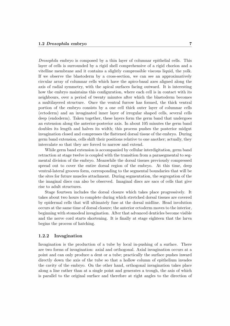
pending on where it takes place. Therefore cells acquire a distinct wedge shape;they are apically constricted when located at the median hinge point, while basallyin the case of dorsolateral hinge point (Fig. 1.3).
Figure 1.3: The hinge points during the invagination process (modified from Davies[2005]).
1.2.3 Ventral furrow Invagination
Ventral furrow invagination (VFI) starts at stage six at the onset of gastrulation; itis one of the most interesting morphogenetic movements in Drosophila Melanogasterfrom a mechanical point of view given the multiple elementary deformations andforces involved.
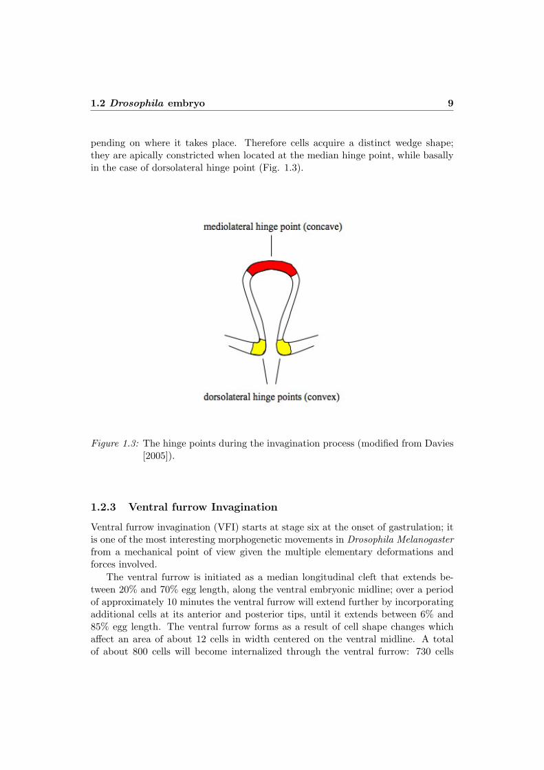
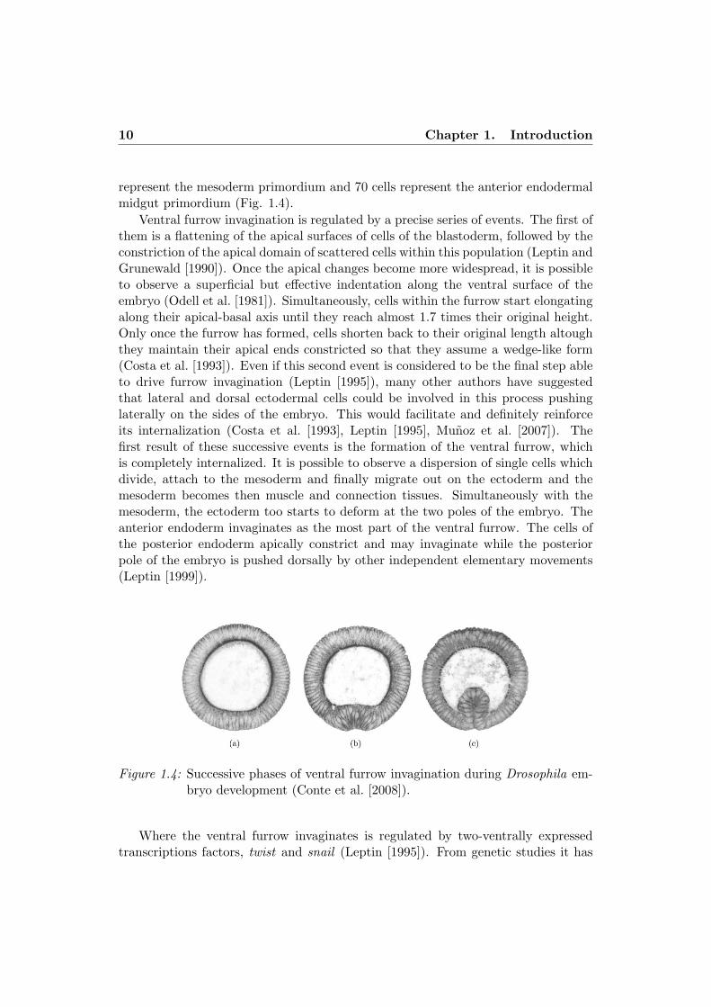
The ventral furrow is initiated as a median longitudinal cleft that extends be-tween 20% and 70% egg length, along the ventral embryonic midline; over a periodof approximately 10 minutes the ventral furrow will extend further by incorporatingadditional cells at its anterior and posterior tips, until it extends between 6% and85% egg length. The ventral furrow forms as a result of cell shape changes whicha!ect an area of about 12 cells in width centered on the ventral midline. A totalof about 800 cells will become internalized through the ventral furrow: 730 cells
10 Chapter 1. Introduction
represent the mesoderm primordium and 70 cells represent the anterior endodermalmidgut primordium (Fig. 1.4).
Ventral furrow invagination is regulated by a precise series of events. The first ofthem is a flattening of the apical surfaces of cells of the blastoderm, followed by theconstriction of the apical domain of scattered cells within this population (Leptin andGrunewald [1990]). Once the apical changes become more widespread, it is possibleto observe a superficial but e!ective indentation along the ventral surface of theembryo (Odell et al. [1981]). Simultaneously, cells within the furrow start elongatingalong their apical-basal axis until they reach almost 1.7 times their original height.Only once the furrow has formed, cells shorten back to their original length altoughthey maintain their apical ends constricted so that they assume a wedge-like form(Costa et al. [1993]). Even if this second event is considered to be the final step ableto drive furrow invagination (Leptin [1995]), many other authors have suggestedthat lateral and dorsal ectodermal cells could be involved in this process pushinglaterally on the sides of the embryo. This would facilitate and definitely reinforceits internalization (Costa et al. [1993], Leptin [1995], Munoz et al. [2007]). Thefirst result of these successive events is the formation of the ventral furrow, whichis completely internalized. It is possible to observe a dispersion of single cells whichdivide, attach to the mesoderm and finally migrate out on the ectoderm and themesoderm becomes then muscle and connection tissues. Simultaneously with themesoderm, the ectoderm too starts to deform at the two poles of the embryo. Theanterior endoderm invaginates as the most part of the ventral furrow. The cells ofthe posterior endoderm apically constrict and may invaginate while the posteriorpole of the embryo is pushed dorsally by other independent elementary movements(Leptin [1999]).
Figure 1.4: Successive phases of ventral furrow invagination during Drosophila em-bryo development (Conte et al. [2008]).
Where the ventral furrow invaginates is regulated by two-ventrally expressedtranscriptions factors, twist and snail (Leptin [1995]). From genetic studies it has

1.2 Drosophila embryo 11
been observed that:
• none of the morphogenetic events that accompany ventral furrow formationoccurs in the absence of twist and snail ;
• the co-expression of twist and snail is su"cient to generate ectopic furrows.
Figure 1.5: The table shows the strong control exerted by the genes twist and snailon ventral furrow invagination. The symbols !/X indicate the activa-tion/repression of the corresponding gene, the presence/absence of thecorresponding cell shape change in the mesodermal primordium or thesuccess/failure of ventral furrow invagination (Conte et al. [2008]).
Twist is a transcriptional activator that plays a common role in every gastrula-tion movements in insects (Roth [2004]). Specifically, it induces the expression, inthe ventral region of the embryo, of Fog and T48 (Kolsch et al. [2007]), that recruitRhoGEF2 a contractile actin/myosin network at apical adherens junctions (Barrettet al. [1997]) to induce apical constriction of the cells. On the other hand, twistincreases the expression of snail, which can actually rescue several defects observedin twist mutant embryos (Costa et al. [1993]). During ventral furrow formationin Drosophila, snail inhibits ectodermal cell fate; in addition it is highly requiredfor apical constriction and may also influence the rearrangement of adherens junc-tions within the epithelial layer (Kolsch et al. [2007], Oda and Tsukita [2000]). Acombination of twist and snail leads to ventral furrow invagination via mechanicalevents such as apical flattening, apical constriction, early apico-basal elongation,late apico-basal shortening and basal wedging (Fig. 1.5). Although only apical con-striction and the signaling pathway inducing it are well understood so far, whileinformation on the other forces involved in ventral furrow invagination still remainunknown or less understood. In particular, it is still di"cult to distinguish, among

12 Chapter 1. Introduction
the deformations mentioned above, the active and the passive processes. The firstones are represented by the forces internal to each cell, which would trigger a puredeformation if the cells were isolated and not part of system, in contact with oneeach other. The second ones instead correspond to the passive response due to theincompatibility generated by the active deformations.
Several experimental observations have been conducted on mutant embryos inwhich particular aspects of the normal morphogenetic process have been geneticallyuncoupled. These studies have provided new information on active forces involved infurrow formation. In twist mutants embryos for example, the cells in the mid-ventralregion elongate to the same length as in the wild type embryos, even if they do notundergo apical constriction or furrow formation. This leads to a thicker mesoder-mal primordium (Leptin and Grunewald [1990]); therefore apico-basal elongation isnot simply a passive response to the apical constriction as nuclei and cytoplasm arepushed basally (Costa et al. [1993]). For what concerns instead snail mutants em-bryo, they show an opposite behaviour. In fact they shorten and generate a thinnermesodermal primordium, even if, also in this case, apical constriction and apicalflattening do not a!ect the final shape of the cells so that it is possible to deduce anindependence between snail and twist (Leptin and Grunewald [1990]). To conclude,it seems reasonable to think that the shape modifications mentioned above are instrong connection with one another and they drive ventral furrow invagination.
1.2.3.1 Modeling of ventral furrow invagination
By previous paragraphs we can easily deduce how biomechanics plays a significantrole during the di!erent phases of embryo development. Therefore, the need moreand more evident of mechanical models and in particular numerical ones, that cancontribute to a complete understanding of the biological system as a whole. Com-puter simulations provide a realistic reproduction of the biological events and maypoint out interesting aspects omitted through experimental observations, so thatnew issues and questions are introduced.
In the last decades, several 2D models have been designed to analyze invagination(also refer to Taber [1995]). The two very first of them (Jacobson and Gordon[1976], Jacobson [1980]) focused on neurulation in the newt using experiments andgeometric analysis. The authors concluded that the deformation occurring is notsimply a rolling into a tube, but there is also an elongation of the neural plate in theanterior-posterior direction as the neural tube forms. Jacobson (Jacobson [1980])also suggested that such elongation may lead to the buckling of the epithelium witha furrow forming along the direction of the stretch engendering eventually the neuraltube.
The work of Odell (Odell et al. [1981]) provides an epithelial model based onapical microfilaments contraction. The main characteristics of the model are:
• the cells in the sheet are tightly bound;

1.2 Drosophila embryo 13
• the cytoplasm is a viscoelastic solid;
• the apical surface of each cell includes a network of microfilaments. Whena small amount of these filaments is stretched, they act as passive viscoelas-tic material, while when a threshold value of stretch is achieved, an activecontractile force is developed, which remains for all time thereafter.
In order to obtain these features, each cell is represented as a four-sided, two-dimensional truss element composed by six viscoelastic units, each of which includesa spring (k) and a dashpot (µ) in parallel (Fig. 1.6). The diagonal componentscorrespond to the cytoskeleton, while the others to the cell membrane. Only theapical unit is able to actively contract.
Figure 1.6: Representation of a cell in the Odell’s model (Odell et al. [1981]).
Each element is governed by the equation
F = k(L! L0) + µL (1.1)
where F is the load applied at the ends, L(t) is the current length and L0(t) isthe inital length of the unit. The activation is obtained letting L0 vary with timeaccording to the following relation
L0 = G(L,L0) (1.2)
where G = 0 for a passive unit. The model behaviour therefore depends on thechoice of G and the authors have chosen a relatively simple form for it, allowing

14 Chapter 1. Introduction
to have two stable equilibrium values for L0: one for the passive zero-stress lengthand the other for the active zero-stress length. The model was tested for amphibiangastrulation, Drosophila furrow formation and amphibian neurulation (Fig. 1.7).It was found that the observed morphology could be obtained by adjusting theactivation parameters in Eq.[1.2].
Figure 1.7: Results for the Odell’s model (Odell et al. [1981]).
Later Oster and Alberch (Oster and Alberch [1982]) used this model to illustrateepithelial bifurcation (change in local or global stability and equilibrium) duringdevelopment. Particularly, they demonstrated how, only by fairly changing the vis-coelastic properties of the cells, they were able to obtain the gastrulation modelbuckling outward rather than inward. This behaviour may influence epithelial mor-phogenesis since invagination engenders hair or skin glands, while evagination leadsto the formation of feathers or scale. Therefore a small variation of some parameterscan induce significant global changes.
In 1986, Jacobson (Jacobson et al. [1986]) proposed a cortical tractor model in
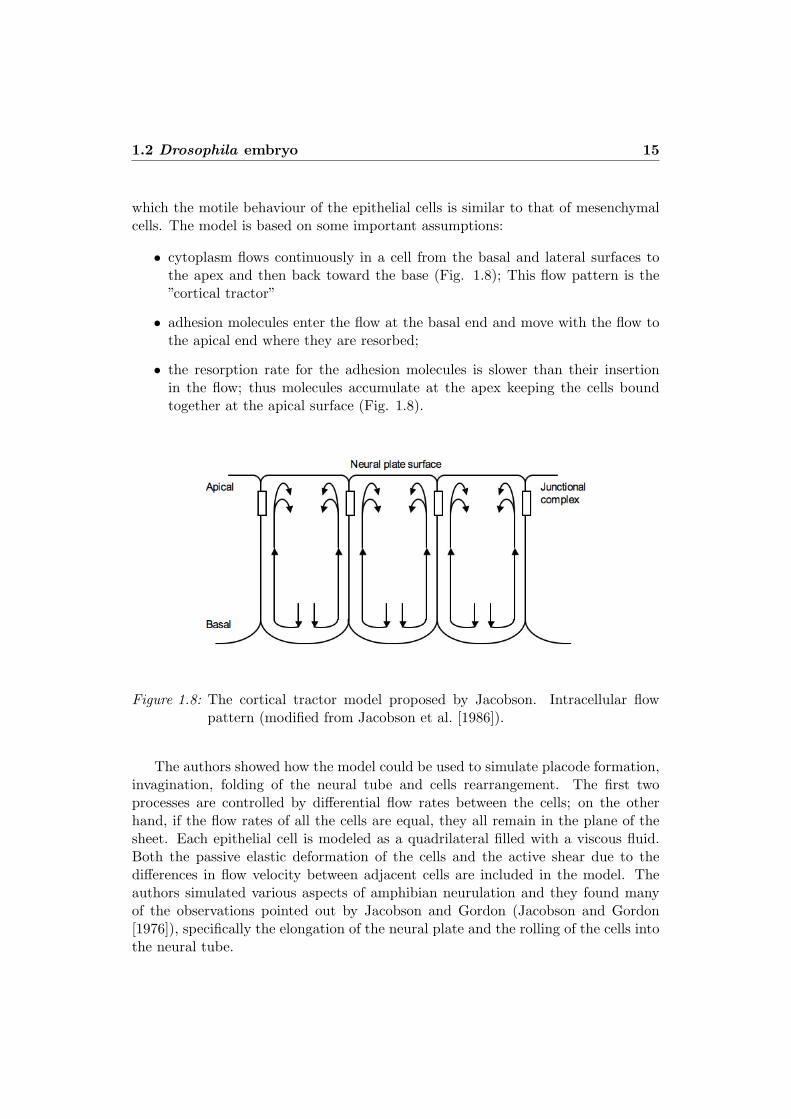
1.2 Drosophila embryo 15
which the motile behaviour of the epithelial cells is similar to that of mesenchymalcells. The model is based on some important assumptions:
• cytoplasm flows continuously in a cell from the basal and lateral surfaces tothe apex and then back toward the base (Fig. 1.8); This flow pattern is the”cortical tractor”
• adhesion molecules enter the flow at the basal end and move with the flow tothe apical end where they are resorbed;
• the resorption rate for the adhesion molecules is slower than their insertionin the flow; thus molecules accumulate at the apex keeping the cells boundtogether at the apical surface (Fig. 1.8).
Figure 1.8: The cortical tractor model proposed by Jacobson. Intracellular flowpattern (modified from Jacobson et al. [1986]).
The authors showed how the model could be used to simulate placode formation,invagination, folding of the neural tube and cells rearrangement. The first twoprocesses are controlled by di!erential flow rates between the cells; on the otherhand, if the flow rates of all the cells are equal, they all remain in the plane of thesheet. Each epithelial cell is modeled as a quadrilateral filled with a viscous fluid.Both the passive elastic deformation of the cells and the active shear due to thedi!erences in flow velocity between adjacent cells are included in the model. Theauthors simulated various aspects of amphibian neurulation and they found manyof the observations pointed out by Jacobson and Gordon (Jacobson and Gordon[1976]), specifically the elongation of the neural plate and the rolling of the cells intothe neural tube.

16 Chapter 1. Introduction
Very often from a macroscopical point of view it is more convenient to representthe epithelium as a plate or a shell, therefore as a continuum; Hardin and Cheng(Hardin and Cheng [1986]) proposed a model in which axisymmetric shell theory wasused to simulate Sea Urchin gastrulation. They analyzed large deformations but theshell material was taken linear and isotropic. They obtained the gastrulation of theepithelium applying forces through the archenteron to opposite sides of a sphericalshell representing the blastula (Fig. 1.9). Since the material properties in the entirestructure are considered uniform, the authors observed a flattening of the blastularoof which is inconsistent with experimental results; furthermore, the model doesnot take into account the internal fluid in the blastula whose pressure may help theclosure of the blastopore which is not obtained here.
Figure 1.9: The shell model for gastrulation proposed by Hardin and Cheng (Hardinand Cheng [1986]).
A limited number of other shell models have been published. Mitthenthal (Mit-thenthal [1987]) used a fluid-elastic thin-shell theory based on the assumption that

1.2 Drosophila embryo 17
the shell resists bending and isotropic in-plane stresses elastically, but it cannot sup-port static shear stresses. Gierer (Gierer [1977]) proposed a model based on adhesivepotential, while Zinemanas and Nir (Zinemanas and Nir [1987]) modeled the blas-tula as a viscous drop of liquid surrounded by a fluid membrane and embedded inan ambient fluid.
Davidson (Davidson et al. [1995]) studied very accurately the forces that drivethe Sea Urchin invagination; he proposed a series of finite elements simulations thattest five hypothesized mechanisms and demonstrated that each one of them cangenerate invagination. The models he proposed are the following:
• an apical constriction model in which an imposed gradient of constriction alongthe cell axis drives the contraction of the apical surface and the expansion ofthe basal surface so that the cell volume remains constant;
• a cell contractor model obtained by appending contractile protrusions to a ringof cells at about 20µm from the center of the plate, a region that includes mostof the cells that participate in primary invagination;
• an apical contractile ring model based on the wound healing mechanism ob-served in Xenofus embryos. A contractile ring of approximatevely 40µm indiameter and centered on the vegetal plate is installed at the apical surface ofthe cell layer; the contraction of this cable triggers both the invagination ofthe plate and the coordinated changes in shape occurring to the cells;
• an apico-basal contraction model in which contractile elements are embeddedacross the thickness of the cell layer within 20µm from the center of the vegetalplate. The forces generated by these contractile units are su"cient to bucklethe epithelial sheet to the correct geometry;
• a gel swelling model where the vegetal plate apical lamina covers the regionwhich normally invaginates and swells isotropically. The vegetal plate, whichis constrained by the surrounding epithelium, buckles inward as the apicallamina expands.
The success of each mechanism depends on the passive sti!ness of the cell layerrelative to the sti!ness of the two extracellular matrix layers. The cell tractoring,the apicobasal contraction and the gel swelling mechanisms work only when theextracellular matrix is very sti! with respect to the cell layer. On the other hand,the apical constriction and the apical contracting ring models work with a moredeformable extracellular matrix.
In 1993 Clausi and Brodland (Brodland and Clausi [1993]) used apical constric-tion as primary driving force in their finite elements model for neurulation. Theyassumed that the microfilament force increases with contraction and they obtainedvery realistic results.

18 Chapter 1. Introduction
We also mention the work of Pouille (Pouille and Farge [2008]) in which anepithelium of cells is immersed in an incompressive viscous fluid. Some structuralelements are used to describe the cell membranes, their actin cortex connected byapical and basal junctions and the apical adherens junctions connected to the con-tractile actin/myosin ring. These units are connected to each other to shape the cellsof the epithelium enclosing the yolk. The cells and the yolk maintain their internalvolumes of incompressible viscous fluid constant. The cell membranes are under thecontractile elastic tension due to the actin/myosin cortex, while the contractibilityof the adherens junctions is obtained putting additional springs crossing the disc.The authors pointed out how only the increase in the apical-cortical surface tensionis the control parameter change required to simulate the main multicellular and cel-lular shape changes in Drosophila gastrulation. Therefore, most of the behavioursobserved in vivo (apical junctions movements at the onset of gastrulation, cell elon-gation and consequent shortening during invagination) appear to be in this model apassive response to the genetically controlled apical constriction of the cells.
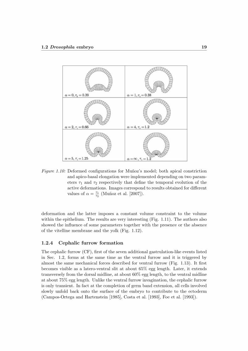
A common feature of all these models is the presence of structural units as actu-ators that reproduce elements of the cytoskleton such as microtubules and microfila-ments. These elements lead the necessary shape changes, mainly apical constrictionor axial elongation on certain region of the embryo. More recently, Munoz (Munozet al. [2007]) proposed a model with no structural elements (Fig. 1.10). He simulatedventral furrow invagination using a deformation gradient decomposition method tomodel the permanent active deformations and the passive hyperelastic deformationsas a local quantity applied to the continuum that schematises the epithelial layer.Each point of the epithelial cell layer is able to reproduce the two main deformationsmodes involved in invagination: apical constriction and apico-basal elongation.
A similar approach was used by Taber (Ramasubramanian and Taber [2006],Taber [2007]) that based his models on the Beloussov’s hyper-restoration hypothe-sis (Beloussov [1998], Beloussov and Grabovsky [2007]) by which morphogenesis isregulated in part by feedback from mechanical stress. According to this hypothesis,active tissue responses to stress perturbations tend to restore, but go beyond theoriginal target stress; the rate of growth or contraction depends on the di!erencebetween the current and the target stresses. He tested several finite elements modelsfor stretching of epithelia, cylindrical bending of plates, invagination of cylindricaland spherical shells and early amphibian development. In each of these cases, aninitial perturbation leads to a mechanical response which changes the global shapeof the tissues.
Conte (Conte et al. [2008], Fig. 1.11) extended the work of Munoz to developthe first three-dimensional model for ventral furrow invagination. The method usedis the same as for the two-dimensional model previously described so that any pointin the epithelial layer can contribute to the global deformation. In the model, thereare no external constraints other than the presence of the vitelline membrane andthe yolk. The former is modelled as a rigid sleeve-shaped shell constraining the
1.2 Drosophila embryo 19
Figure 1.10: Deformed configurations for Munoz’s model; both apical constrictionand apico-basal elongation were implemented depending on two param-eters !1 and !2 respectively that define the temporal evolution of theactive deformations. Images correspond to results obtained for di!erentvalues of " = !1
!2(Munoz et al. [2007]).
deformation and the latter imposes a constant volume constraint to the volumewithin the epithelium. The results are very interesting (Fig. 1.11). The authors alsoshowed the influence of some parameters together with the presence or the absenceof the vitelline membrane and the yolk (Fig. 1.12).
1.2.4 Cephalic furrow formation
The cephalic furrow (CF), first of the seven additional gastrulation-like events listedin Sec. 1.2, forms at the same time as the ventral furrow and it is triggered byalmost the same mechanical forces described for ventral furrow (Fig. 1.13). It firstbecomes visible as a latero-ventral slit at about 65% egg length. Later, it extendstransversely from the dorsal midline, at about 60% egg length, to the ventral midlineat about 75% egg length. Unlike the ventral furrow invagination, the cephalic furrowis only transient. In fact at the completion of germ band extension, all cells involvedslowly unfold back onto the surface of the embryo to contribute to the ectoderm(Campos-Ortega and Hartenstein [1985], Costa et al. [1993], Foe et al. [1993]).

20 Chapter 1. Introduction
Figure 1.11: The first 3D model of ventral furrow invagination provided by Conte(Conte et al. [2008]). Three deformed configurations show respectivelya ventral view (a, c, e) and a cross sectional view (b, d, f).
Figure 1.12: Simulations with the modified boundary conditions and unusual activedeformations (Conte et al. [2008]). (a, b) Simulations where no vitellinemembrane is considered, 2D section (a) and 3D view (b). (c, d) Resultswhen yolk pressure was not implemented, 2D section (c) and 3D view(d). (e, f) Simulations where apico-basal elongation was not considered,2D section (e) and 3D view (f).

1.2 Drosophila embryo 21
Figure 1.13: The formation of the cephalic furrow at the anterior end of a developingDrosophila Melanogaster embryo visualized with the help of severalfluorescent stains (www.invitrogen.com).
Even though the cephalic furrow is a prominent morphological event of the earlygastrula, its developmental role remains enigmatic (Vincent et al. [1997]). It hasnot been possible so far to isolate specific mutations a!ecting only this event; fur-thermore” the cellular and genetic mechanisms that control its formation are stillunknown. Eventually, the absence of a cephalic furrow in embryos derives frommothers mutant for bicoid (Frohnhofer and Nusslein-Volhard [1986]) and the repro-ducible shifts in its position and its lateral extent indicates that the cell shape isdirectly a!ected by positional information (Zusman and Wieshaus [1985]). Never-theless, these particular information do not provide interesting tips on how positionalinformation are translated into specific changes in cellular morphology.
The cephalic furrow forms at an interesting region of the embryo, at the jux-taposition of the patterning systems that define the head and the trunk segments;these two systems involve di!erent groups of zygotically active genes, specificallycephalic furrow coincides with the expression of the pair-rule gene eve and it hasbeen observed (Costa et al. [1993]) that in eve mutant embryos the cephalic furrow iseliminated or abnormal, which suggests a strong control of eve on the morphogeneticevent. In addition, the activity of the head gap-like segmentation gene buttonheadmay also influence the formation of the furrow (Vincent et al. [1997]).
The lack of accurate information has definitely restrained mechanical modelingof the cephalic furrow formation even if it represents one of the most interesting

22 Chapter 1. Introduction
morphogenetic event in Drosophila embryo. Therefore, the present work is originalin this sense since it provides an innovative finite elements model able to simulatethe formation of the furrow.
1.2.5 Convergence-extension movements
During morphogenesis, epithelial tissues undergo changes in shape very rapidly andoften cell division does not play a role in this process. More particularly, tissuesseem to behave like membranes that stretch and bend; usually these mechanicalmovements are accompanied by a change in shape of individual cells or by a rear-rangement of the cells so that they change their neighbours.
1.2.5.1 Occurrence of the convergence-extension
The convergence-extension is a key process leading to the formation of an elongatedaxis in many animal phyla (Kimmel et al. [1994], Schoenwolf and Alvarez [1989]).Also it can take place in epithelial tubes as in the case of the Sea Urchin, whereonce the gut has formed, the cells around its circumference decrease, while thenumber along its length increases (Davies [2005]). For sure, one of the most studiedexamples is the elongation of the germ band in Drosophila Melanogaster (Irvine andWieschaus [1994]), which we are going to describe and analyze more in details inthe next section.
Convergence and extension are normally used to indicate the narrowing and thelengthening of tissues respectively (also refer to Keller et al. [1991b] and Keller et al.[1991a]). Convergence can be coupled directly to extension with conservation oftissue volume, therefore a decrease in width occurs with a proportional increase inlength. In other cases, convergence may engender thickening as well as lengthening.Thus the term ”convergence-extension” is often used for convenience, but one has toremember and consider the complex relationship between convergence, extension andthickening. Actually, convergence-extension movements can be included in a largerand more general class of ”mass movements”, involving change in tissue proportionswith approximate conservation in volume (Keller et al. [2000]). In addition, thesetype of movements may be a passive response to forces generated elsewhere in theembryo or they may be active and force-producing processes.
These ”mass movements” represent a very interesting challenge and also a greatopportunity to better understand the functions of the cells with respect to embryoge-nesis. So far, little is known about the cellular, molecular and biological mechanismsof these movements so that it is not easy at all to evaluate their role and importancein shaping the embryo’s body. Furthermore, cell interactions within populations aredi"cult to detect since it is di"cult to visualize and interpret cell motility throughthe embryo. In fact, the functions of the cells are usually studied on individual cellsin culture at low density, while most of mass movements take place at high densities

1.2 Drosophila embryo 23
of cells that are interacting with one another or with the extracellular matrix. Fi-nally it has also to be noticed that in the case of a single cell, the generated forceshave local e!ects on its movement in culture; for cells populations instead, theseforces have both local e!ects and e!ects that are integrated through the population.
1.2.5.2 Cell rearrangement or intercalation
In most of the cases, convergence-extension movements are triggered by the re-arrangement of the cells; practically the cells intercalate between one another toproduce a significant change in shape of the tissue and then to form a sti! array,which can distort and deform the surrounding passive tissues (Fig. 1.14).
The first who supposed this type of process was Waddington in 1940 (Wadding-ton [1940]); by studies on amphibians, he observed that the convergence-extensionoccurred in absence of cell growth and the appropriate changes in shape, thereforehe suggested that these movements must take place by cells rearrangement.
Figure 1.14: Cells rearrangement process during convergent-extension movement.
The regions involved in these ”mass movements” are composed by a single layerof superficial epithelial cells and several layers of deep mesenchymal cells. Morpho-logical studies have shown that tissues converge and extend by two main types ofcells rearrangement. During the first half of gastrulation, mesenchymal cells andposterior neural tissues undergo radial intercalation (Keller [1980]); they intercalate

24 Chapter 1. Introduction
along the radius of the embryo, normal to its surface, to generate a thinner array thatis also longer in the prospective anterior-posterior axis. Usually superficial epithelialcells do not participate to this phase of intercalation, but simply spread and divideto accommodate the larger area of the spreading deep cells. Just after radial inter-calation, convergence-extension occurs by a mediolateral intercalation in which cellsmove between one another to form a narrower, longer and thicker array (Keller andTibbetts [1989]). This time the superficial cells accommodate the narrowing andthe extension of the deeper cells intercalating, dividing and spreading themselvestoo. Usually, mediolateral intercalation occurs at and beyond the blastoporal lip inthe post-involution region, while radial intercalation is typical of the pre-involutionregion.
1.2.6 Cells rearrangement models
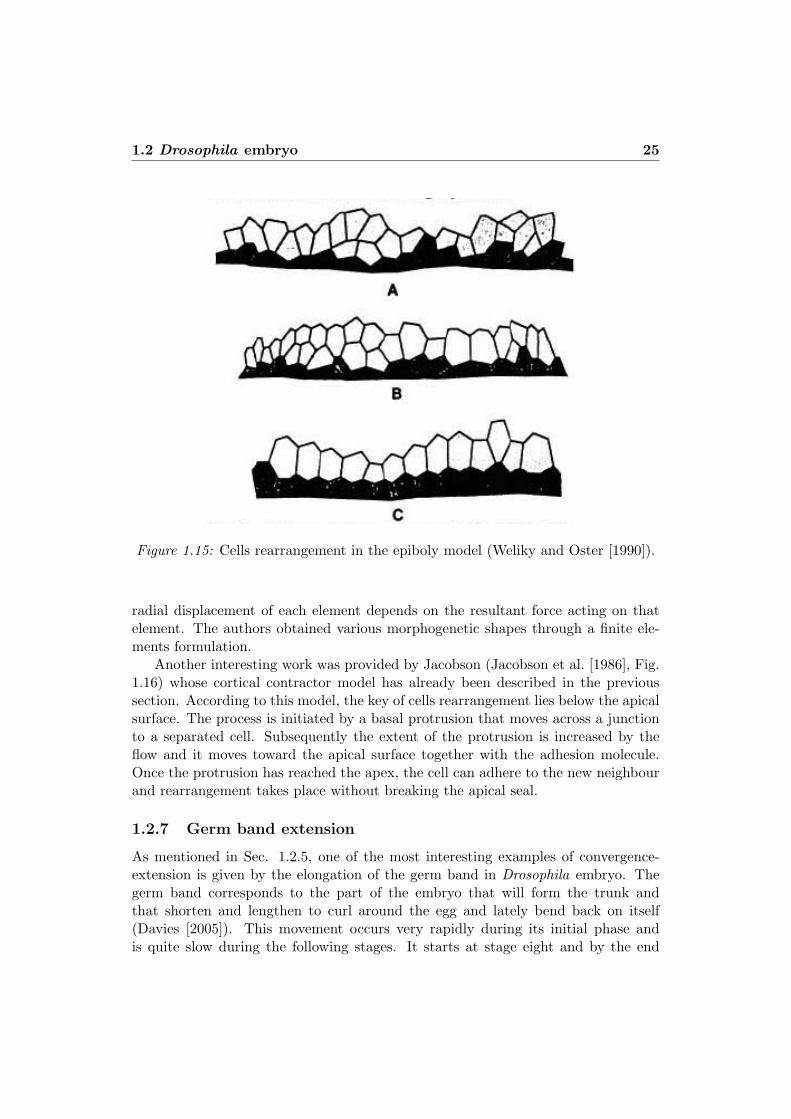
Modeling cells rearrangement within an epithelium is complicated by the need tofollow individual cells. Weliky and Oster (Weliky and Oster [1990]) proposed a sim-ulation for epithelial cells rearrangement taking into account the e!ects of changingintra and intercellular forces. In their model, each cell is represented by a two-dimensional polygon with a variable number of sides and nodes that can slide, ap-pear and disappear (Fig. 1.15). The forces applied on the node determine its motionand, to maintain the compatibility, the geometry is updated. The plasma membraneof each cell contains actin/myosin filaments and encloses a filament-rich gel. Theforces generated on the nodes may be caused by:
• positive osmotic pressure that expands the gel;
• negative elastic pressure due to intracellular filaments opposing gel swelling;
• tension in the sides due to microfilament bundle contraction;
• external loads.
Each node moves proportionally to the force acting on it and in the direction ofthe resultant force; therefore internal pressure triggers protrusions while tensile wallstress drives cellular contraction. The model was used to simulate epiboly (when anepithelium expands to enclose the interior of the early embryo) and it was observedthat the number of cells at the margin decreases continually during the process evenif its circumference increases.
The model was later modified by Weliky (Weliky et al. [1991]) with some newfeatures to analyze tissue extension, cell rearrangement and the interactions of cellswith boundaries. The conclusion was that several rules of cell behaviour operatesimultaneously during frog neurulation.
Beloussov and Lakirev (Beloussov and Lakirev [1991]) used a very similar ap-proach modeling the epithelium as a shell composed by movable elements. The
1.2 Drosophila embryo 25
Figure 1.15: Cells rearrangement in the epiboly model (Weliky and Oster [1990]).
radial displacement of each element depends on the resultant force acting on thatelement. The authors obtained various morphogenetic shapes through a finite ele-ments formulation.
Another interesting work was provided by Jacobson (Jacobson et al. [1986], Fig.1.16) whose cortical contractor model has already been described in the previoussection. According to this model, the key of cells rearrangement lies below the apicalsurface. The process is initiated by a basal protrusion that moves across a junctionto a separated cell. Subsequently the extent of the protrusion is increased by theflow and it moves toward the apical surface together with the adhesion molecule.Once the protrusion has reached the apex, the cell can adhere to the new neighbourand rearrangement takes place without breaking the apical seal.
1.2.7 Germ band extension
As mentioned in Sec. 1.2.5, one of the most interesting examples of convergence-extension is given by the elongation of the germ band in Drosophila embryo. Thegerm band corresponds to the part of the embryo that will form the trunk andthat shorten and lengthen to curl around the egg and lately bend back on itself(Davies [2005]). This movement occurs very rapidly during its initial phase andis quite slow during the following stages. It starts at stage eight and by the end

26 Chapter 1. Introduction
Figure 1.16: Cellular rearrangement mechanism (Jacobson et al. [1986]).
of stage ten the elongation has progressed to bring the posterior tip of the germband to about 75% egg length. Meanwhile the cells converge from the dorsal tothe ventral region of the embryo and intercalate between one another so that thetissues elongate along the midline. During the process, the cells never acquire freeedges, therefore the integrity of the epithelium is retained. Particularly before theconvergence-extension movement, the cells form an hexagonal array, while after therearrangement the centers of the cells form ordered rows along the anterior-posterioraxis. This means that one third of the cell-cell boundaries are at 90! with respectto the anterior-posterior axis, one third at 30! and the remaining at -30!.
The intercalation of the cells is highly directional since cells intercalate almost ex-clusively between dorsal and ventral neighbours and only rarely between anterior andposterior neighbours (Irvine and Wieschaus [1994]). Although evenly distributed, in-tercalation does not follow a precise pattern given that blastoderm neighbours maybe separated by zero, one, two or three cells. Furthermore, cells only intercalatebetween their nearest neighbours and do not migrate widely; this can be observedfollowing columns that extend from dorsal to ventral. These columns become shorterand wider as the germ band extends and when they collapse into irregular shape,the cells of a single column always remain together.
The cells first move slightly dorsally, then more rapidly ventrally and posteriorlyand finally simoultaneously posteriorly and ventrally. The positioning of the cellsmay a!ect the trajectories; in fact more dorsal cells move further ventrally than
1.3 Conclusions 27
ventral cells do and more posterior cells move further posteriorly than anterior cellsdo. In addition cells that are near the cephalic furrow first move anteriorly push-ing the furrow forward and then they start moving posteriorly (E. Wieschaus andKluding [1984]). Intercalation is symmetrical since dorsal cells come between theirventral neighbours and ventral cells come between their dorsal neighbours. There isan increase in the number of cells along the anterior-posterior axis, which is morerapid ventrally than dorsally, and a decrease along the dorsal-ventral axis.
Even if it has not been possible so far to individuate mutations that are specifi-cally defective of germ band extension, mutations in many of the genes involved inpatterning along the anterior-posterior axis have shown reduction of the elongation.In particular the process is reduced by mutations in the maternal coordinate genesand in the zygotic gap and pair-rule segmentation genes; specifically eve seems tomostly reduce the extension of the germ band (Irvine and Wieschaus [1994]).
1.3 Conclusions
Embryogenesis is a very complex process where mechanics and biology are mergedtogether, with strong interconnections at di!erent phases of the development. Iffor a long time biologists have observed the influence of genetics on the mechani-cal forces within the embryo, as largely described in the previous paragraphs, onlyrecently they have supposed the inverse phenomenon: the control exerted by me-chanics on the expression of specific genes. It is still not so clear and understood howa mechanical force can be transformed into a chemical signal, but it is evident thata mechanotransduction pathway must be present all long the embryogenesis. Also,embryonic cells, as other types of cells in nature (endothelial cells, muscle cells...),must be mechanosensible and therefore able to deform and to adapt themselves whenexternal loads are applied on them.
Each cell is characterized by the presence of internal elementary forces, the pri-mary or active forces, that can occur during embryo development and would lead toa pure deformation if cells were not part of a system and in contact with one eachother. Instead, boundary conditions at the interfaces must be respected, therefore,to avoid the incompatibility (i.e. superposition of volumes) potentially caused by theelementary forces, tissues are forced to deform again (secondary or passive forces)in order to maintain the continuity of the mesoderm. For the three morphogeneticmovements we have decided to focus on (ventral furrow invagination, cephalic furrowformation and germ band extension), several elementary forces have been individu-ated by biologists, but so far it is still di"cult to determine which ones among themcan be considered a real primary force and which ones a simple passive responseof the neighbour cells to the active ones. Mechanical modeling, and numerical onein particular, may help in detecting this peculiar aspect, as we are going to showlater on, other than provide a useful tool in investigating more accurately the global
28 Chapter 1. Introduction
response of the embryo to mechanical forces.That being said, treating with a biological system always represents a real chal-
lenge. Many are the parameters that may a!ect the global behaviour of the structureand most of the time they are very di"cult to detect. Additionally, for our specificcase, the embryo is composed by several elements not easy to model, therefore manyapproximations are made so that the final representation is often a macro-scale rep-resentation.
The di!erent works we have found in literature and briefly described in thischapter prove the progresses that have been made in computer simulation in thelast decades. The methods and approaches used are all very interesting and supplyconsistent results compared to the biological observations. Nevertheless we thinkthat our model, which have been first presented at the Second International Confer-ence on Mechanics of Biomaterials and Tissues (Hawaii, 9-13 December 2007), showssome innovative aspects with respect to the previous ones (Allena et al. [2008]).
Most of the former works have been conceived in a two dimensional space, whileour description of the embryo is done in a three dimensional space, so that we havea more realistic representation of the biological reality. In despite of this it has tobe noticed that the geometry of our model has not been obtained from MRI, but anellipsoid has been used to represent the embryo, thus the di!erent curvature betweenthe anterior and the posterior pole is not considered here. We are aware that thischaracteristic may influence the final results, especially for the simulation of thosemovements that take place along the anterior-posterior axis (i.e. ventral furrowinvagination and germ band extension). Also only mesoderm has been modelledassuming that the mechanical characteristics of the three embryonic layers, whichform throughout the gastrulation phases, may not be so di!erent so that we canconsider that the mesoderm constitutes the most part of the blastoderm.
With a single model and without introducing any structural elements, we are ableto individually simulate three morphogenetic movements: ventral furrow invagina-tion (VFI), cephalic furrow (CF) formation (which, to the best of our knowledge, hasnever been simulated before) and germ band extension (GBE). This is possible bythe parametrical description of the embryo which constitutes the outstanding advan-tage of the present work with respect to previous ones where the model allowed tosimulate only one movement and most of the time ventral furrow invagination. Ac-tually, we have precise active deformation gradients, according to the morphogeneticmovement analyzed, that are analytically obtained and can easily be changed andelaborated. Furthermore” the active forces we introduce are independent of the meshapplied on the geometry and thus of the discretization.
Finally we will present here not only the simulation of the three movementsindividually, but also and more importantly the concurrent simulation of two orthree of them. This represents a very innovative feature because, to the best of ourknowledge, it is the first time that the three movements are coupled together. Theconcurrent simulation provides a more complete view of a fragment of Drosophila

1.3 Conclusions 29
embryogenesis, the gastrulation, which is one of the most complex and interestingphase of the developmental process.
The main goal of the present work is therefore to confirm, through the finiteelements model, the hypothesis made by the biologists. Most importantly we provehow mechanical modeling can be helpful not only in clarifying the whole biologicalproblem but also and especially in pointing out some of its facets that have been sofar ignored or rarely developed.

30 Chapter 1. Introduction
Chapter 2
The kinematic model
In this section of the work, we present the general kinematics of the active and passivedeformations that will be described more in detail for each morphogenetic movementin the next chapter. As similarly as previous studies, a gradient decompositionmethod is applied (Sec. 2.1), so that both the active and the passive deformationsundergone by the embryonic tissues are taken into account and, coupled together,provide the final deformation. Additionally, we show some interesting interpretationsof the approach and we point out novel aspects of the problem that lead to furtherdiscussions. Specifically, in Sec. 2.4 we compare the gradient decomposition to anequivalent thermal deformation, while in Sec. 2.5 we analyze the potential e!ects ofthe local active forces on both the active and passive domains and in particular atthe internal and external cellular interfaces.
The Virtual Power Principle is then used to write the equilibrium of the system(Sec. 2.2) for which, other than the internal forces of the structure, we must take intoaccount the boundary conditions. We implement the contact between the epithe-lial layer and the external semi-rigid membrane (Sec. 2.7.1) and the yolk pressureexerted on the internal surface of the embryo (Sec. 2.7.2). The presence of thesetwo components, even if not geometrically represented here, is necessary to obtainrealistic final configurations. The model has been validated by testing it on simplegeometries in two or three dimensions (Sec. 2.6).
In Sec. 2.3, we focus on the constitutive law used to describe the embryonictissues. A Saint-Venant model is proposed for the present work which may not bethe best representation compared to the Neo-Hookean material used by previousauthors. A comparison between the two models is made; the results obtained forboth cases show similar results (Chapter 3), so that our choice can be consideredappropriate even if presenting some limitations.
31
32 Chapter 2. The kinematic model
2.1 Gradient decomposition method
The model we use for our simulations does not present any structural elementsas other previous works (Chapter 1), but we impose the kinematics of the mainobserved active deformations in Drosophila embryo according to the morphogeneticmovement considered. Onto this active part, a passive deformation takes place,which determines the integrity and the static equilibrium of the embryo. The activedeformation can be identified with the biological impulse of each cell to change itsshape when stimulated by a higher concentration of actin/myosin filaments. If thecells were not part of a system, therefore in contact with one another and constrainedby the presence of the yolk and the vitelline membrane, we would obtain a freedeformation, as if they were isolated, which means that only the active deformationwould be observed. On the other hand, the boundary conditions, imposed by thestructure of the embryo, lead to an auxiliary deformation, the passive one, thatprovides the final configuration observed. The method presented here has alreadybeen tested with success for the analysis of ventral furrow invagination in Drosophilaembryo (Ramasubramanian and Taber [2006], Munoz et al. [2007], Conte et al.[2008]). In our model, we do not take into account the causes for the implementedactive deformations, but, contrarily, we consider them as an internal contribution,specifically chemo-mechanically transduced, that can produce di!erent combinationsof the deformations observed through the embryo, as proposed by Munoz (Munozet al. [2007]). Furthermore only the contact between the embryonic tissues andthe vitelline membrane and the yolk pressure have been introduced as boundaryconditions. Later on we will discuss more in detail these two aspects that play animportant role and may influence the global behaviour of the embryo; particularly, ithas been demonstrated that the absence of one of these components provides resultsthat do not match with experimental observations (Conte et al. [2008]).
We assume here that each point of the region where the mechanical transforma-tions are introduced is able to produce the main modes of deformation. The initialconfiguration before any force applied is a stress-free configuration, even if at thispoint some internal stress may develop. From this initial configuration, the activeand the passive deformations are obtained.
As previously mentioned and later on more specified, only the mesoderm hasbeen represented and it has been considered as a regular assembling of cells thatpresent the same geometry. At the reference configuration, in a curvilinear systemof coordinates, by the position of each point p0(#1, #2) on the middle surface of themesoderm, we obtain all the points p(#1, #2, #3) within the thickness of the tissue asfollows
p = p0 + $ n0 (2.1)
where $ is the distance between p and p0 calculated along the normal n0 to the
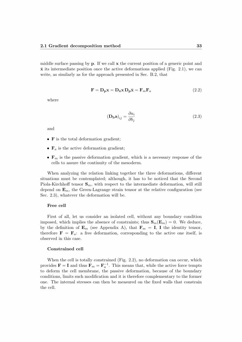
2.1 Gradient decomposition method 33
middle surface passing by p. If we call x the current position of a generic point andx its intermediate position once the active deformations applied (Fig. 2.1), we canwrite, as similarly as for the approach presented in Sec. B.2, that
F = Dpx = DxxDpx = FmFa (2.2)
where
(Dba)ij =%ai
%bj(2.3)
and
• F is the total deformation gradient;
• Fa is the active deformation gradient;
• Fm is the passive deformation gradient, which is a necessary response of thecells to assure the continuity of the mesoderm.
When analyzing the relation linking together the three deformations, di!erentsituations must be contemplated; although, it has to be noticed that the SecondPiola-Kirchho! tensor Sm, with respect to the intermediate deformation, will stilldepend on Em, the Green-Lagrange strain tensor at the relative configuration (seeSec. 2.3), whatever the deformation will be.
Free cell
First of all, let us consider an isolated cell, without any boundary conditionimposed, which implies the absence of constraints; thus Sm(Em) = 0. We deduce,by the definition of Em (see Appendix A), that Fm = I, I the identity tensor,therefore F = Fa: a free deformation, corresponding to the active one itself, isobserved in this case.
Constrained cell
When the cell is totally constrained (Fig. 2.2), no deformation can occur, whichprovides F = I and thus Fm = F"1
a . This means that, while the active force temptsto deform the cell membrane, the passive deformation, because of the boundaryconditions, limits such modification and it is therefore complementary to the formerone. The internal stresses can then be measured on the fixed walls that constrainthe cell.

34 Chapter 2. The kinematic model
Figure 2.1: Initial, intermediate and final configuration for a cell of the embryo.
Figure 2.2: The case of a cell constrained along its boundaries.
Neighbour cells
Finally, we consider the case of a cell whose displacements are limited by thepresence along its boundaries of deformable structures (Fig. 2.3), as similarly as

2.1 Gradient decomposition method 35
for the embryo, where the cells are in contact with one another, with the yolk andthe vitelline membrane and must maintain the integrity of the mesoderm. In thisspecific case, Fm is the actual response to the active deformation Fa, so that thetwo deformations are composed together to provide the suitable final configuration.
Figure 2.3: The case, as similarly as for the embryo, where the cells are in contactwith one another and with some internal or external components.
Fa gives the elementary cell deformations according to the morphogenetic move-ment analyzed and it can be written as
Fa =%x%p
(2.4)
It has to be said here that the active deformation involves the cell membrane andit has therefore to be considered as a micro-scale deformation; for the present studywe have decided to model it as a uniform deformation of the cell. Also, not all thecells of the mesoderm are active at same time and at same regions; thus, accordingto the morphogenetic movement, the elementary deformations will be applied onrestricted domains of the embryo, as it will be shown in Chapter 3, so that we willhave Fa = I elsewhere.
By the tensorial product, we can actually obtain an equivalent expression ofEq.[2.4], which is
Fa =!
m=1,3
%x%pm
" im (2.5)
Because of the curved geometry of the embryo, a special curvilinear coordinatessystem will be employed in Chapter 3, therefore we develop here the necessaryabstract tools.
By the usual convention of the repeated dummy subscript, we know that
36 Chapter 2. The kinematic model
%x%pm
=%x%#n
%#n
%pm(2.6)
thus we find the following formulation for Fa
Fa =!
n=1,3
%x%#n
"!p#n (2.7)
For instance, "x"#1 is the tangent vector at the point
"#10 , #
20 , #
30
#to the curve
(#11 , #
20 , #
30) and, together with "x
"#2 and "x"#3 , which are obtained by circular permu-
tation, constitutes the covariant basis in x. On the other hand, the component#p#1 is the gradient to the surface #1 = #1
0 and forms, with #p#2 and #p#2, thecontravariant basis in p (Smith [1993]). Afterwards we will indicate the former asgx,n and the latter as gn
p. Then we can write
Fa = gx,n " gnp (2.8)
and if no active initial deformation is introduced into the system (Fig. 2.4),p = x and we have
gp,n " gnp = I (2.9)
Without inverting the active configuration from the initial one, we would liketo find the vectors gn
p. The covariant and contravariant basis are related by theequation
(gmp ,gp,n) = &mn (2.10)
and, in an orthogonal basis, for instance for #3, we know that
%#3
%#1=
%#3
%pn
%pn
%#1= (#p#3)n(gp,1)n =
$#p#3,
%p%#1
%= (g3
p,gp,1) (2.11)
so that g3p is perpendicular to gp,1 and, similarly, to gp,2. Consequently, it can
be expressed as
g3p = "(gp,1 $ gp,2) (2.12)
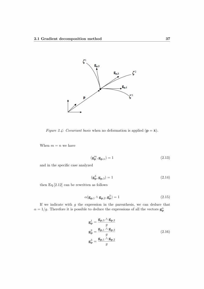
2.1 Gradient decomposition method 37
Figure 2.4: Covariant basis when no deformation is applied (p = x).
When m = n we have
(gmp ,gp,n) = 1 (2.13)
and in the specific case analyzed
(g3p,gp,3) = 1 (2.14)
then Eq.[2.12] can be rewritten as follows
"(gp,1 $ gp,2,g3p) = 1 (2.15)
If we indicate with g the expression in the parenthesis, we can deduce that" = 1/g. Therefore it is possible to deduce the expressions of all the vectors gn
p
g1p =
gp,3 $ gp,2
g
g2p =
gp,1 $ gp,3
g
g3p =
gp,1 $ gp,2
g
(2.16)

38 Chapter 2. The kinematic model
Typically, Fa will be calculated in the special curvilinear coordinates systemadapted to the geometry of the embryo, where active elementary deformations suchas apical constriction, apico-basal elongation and convergent-extension will be in-troduced. In particular we will obtain di!erent expressions of Fa, proper to eachmorphogenetic movement considered, since the intermediate position x changes ac-cording to the deformations applied to the continuum. We will analyze more indetail in the following chapter what happens for the specific cases of the ventralfurrow invagination (Sec. 3.2), the cephalic furrow formation (Sec. 3.2) and thegerm band extension (Sec. 3.3).
2.2 The Principle of the Virtual Power
The Principle of the Virtual Power that we use here is a variational principle withonly one field of dependent variables, specifically the displacement vector u. Thesetype of principles are fundamental and essential in establishing finite elements for-mulations (Holzapfel [2000]). Mechanical systems, all the more so biological systems,are often constituted by heterogeneous materials, which implies the presence of adiscontinuity of the mechanical properties. Particularly, it is necessary to imposesome boundary conditions such as the continuity of the displacements and the reci-procity of the stress vectors; the Principle of the Virtual Power allows the user toautomatically take into account the latter aspects.
If #mx indicates the mesoderm domain at the actual configuration, with %#mix
and %#mexthe internal and the external boundaries respectively (further on the
subscript x will indicate the deformed configuration), the equilibrium of the systemcan be written as
Divx! + 'xfv = 0 in#mx (2.17)
with ! the Cauchy stress tensor and fv the body forces. When considering largedeformations, we do not exactly know the deformed configuration and consequentlywhere the boundary conditions are applied, therefore it is useful to rewrite theequilibrium with respect to the initial configuration. It has to be known that, by theprinciple of mass conservation, the mass density should satisfy the following relation
'x ='
J(2.18)
where J = DetF and ' is the mass density at the initial configuration.Then, classically, the first term of Eq.[2.17] can be rewritten as
Divx! =1JDivp(J!F"T ) =
1JDivp" (2.19)

2.2 The Principle of the Virtual Power 39
with " the First Piola-Kirchho! tensor. Thus Eq.[2.17] becomes
Divp" + ' fv = 0 (2.20)
Here we neglect the volume forces such as gravity, therefore we obtain
Divp" = 0 (2.21)
For two vectors (a,b), we define the dot product as
(a,b) =!
i=1,2
aibi (2.22)
In order to get the Principle of the Virtual Power, we multiply the equilibriumequation (Eq.[2.21]) for a virtual displacements field w so that, by the property ofthe divergence, we have
(Divp",w) = divp""T (w)
#! Tr("DpwT ) (2.23)
and, by integrating over the mesoderm domain #m at the reference configuration,we obtain
&
!m
(Divp",w) =&
!m
divp""T (w)
#!
&
!m
Tr("DpwT ) = 0 (2.24)
By the Stoke’s formula we can write
&
!m
divp""T (w)
#=
&
!m
("T (w),n) =&
"!m
(w,"(n))dS (2.25)
therefore
&
!m
Tr("DpwT ) =&
"!m
(w,"(n))dS (2.26)
We also know that (Holzapfel [2000], Smith [1993])
"(n)dS = !(nx)dSx = fs(nx)dSx (2.27)

40 Chapter 2. The kinematic model
where fs is the modulus of the real surface forces that are supposed to belike normal pressures on the boundaries of the system. We know that (nx)dSx =J F"T (n) dS, thus we can substitute in Eq.[2.27] and then in Eq.[2.26] to obtain
&
!m
Tr("DpwT ) =&
"!m
(w, fsJ F"T (n))dS (2.28)
The term on the right hand side bunches all the external loads acting on theexternal (%#me) or internal (%#mi) boundaries of the mesoderm; we will analyzelater on in this chapter such loads (Sec. 2.7). On the left hand side instead, theinternal forces of the mesodermal domain #m are represented.
The First Piola-Kirchho! tensor, appearing on the left hand side term of Eq.[2.28],can actually be written as
" = FS (2.29)
where S is the Second Piola-Kirchho! tensor, which is equal to
S = J F"1!F"T
= JmJaF"1m F"1
a !F"Tm F"T
a
(2.30)
where Jm and Ja are the determinants of the passive deformation of the meso-derm Fm and of the active deformation Fa respectively. Knowing that
! = J"1m FmSmFT
m (2.31)
where Sm is the Second Piola-Kirchho! tensor with reference to the intermediateconfiguration, which will define the constitutive law of the mesoderm (see Sec. 2.3)and is expressed as in Eq.[2.35], Eq.[2.30] becomes
S = JaF"1a SmF"T
a = Sa (2.32)
From the previous equation, it has to be noticed that the Second Piola-Kirchho!tensors are the same for the active and the final configurations, while we can notstate the same for the First Piola-Kirchho! tensors. In fact we write
"a = FaSa = JaSmF"Ta (2.33)
for the active deformation, which is di!erent from the tensor for the final defor-mation that can be deduced substituting Eq.[2.32] in Eq.[2.29], so that we find
2.3 The constitutive law of the mesoderm 41
" = JaFmSmF"Ta = Ja"mF"T
a (2.34)
We can conclude that " is directly function of the active deformation Fa andthe passive deformation Fm through Sm. As previously mentioned (Sec. 2.1) andlater on described (Chapter 3), Fa depends on the elementary forces introduced andtherefore changes according to the morphogenetic movement analyzed.
2.3 The constitutive law of the mesoderm
As described in Chapter 1, the structure of the Drosophila embryo is rather complexsince, by the beginning of gastrulation, three di!erent tissue layers start to form:an endoderm, an ectoderm and the mesoderm, which is located between these two.So far it has been very di"cult to detect the mechanical characteristics of biologicaltissues (Davidson et al. [1999] and Forgacs et al. [1998]). It seems that embryonictissues are more linear than mature tissues and they also appear to behave as visco-elastic materials during embryogenesis (Forgacs et al. [1998]). For the present workwe have decided to not consider the visco-elastic e!ects, even if we are aware thatthey may highly influence the global response of the system. Furthermore, onlythe mesoderm has been modelled here, as similarly as many finite elements modelsdescribed in Sec. 1.2.3.1 and 1.2.6. We assume in fact that the mechanical character-istics of the three embryonic tissues may not be so di!erent and that the mesodermtakes up the most part of the embryo tissues.
We hypothesized that the mesoderm is made of a Saint-Venant material whoseconstitutive law is written as
Sm = (LTr EmI + 2 µLEm (2.35)
with Em the Green-Lagrange elastic strain of the mesoderm defined as
Em =12
"FT
mFm ! I#
(2.36)
and (L and µL are the Lame’s constants
(L =E )
(1 + ))(1! 2 ))
µL =E
2 (1 + ))
(2.37)
where E is the Young’s modulus and ) the Poisson’s coe"cient. This approachmay not be the best accurate for our specific case; additionally, previous authors
42 Chapter 2. The kinematic model
(Munoz et al. [2007], Taber [2007], Conte et al. [2008]) used a Neo-Hookean materialto reproduce the mesoderm. Such model is a particular case of the Mooney-Rivlinmaterial whose constitutive law can be written as follows
! = "1FmFTm + "2(FmFT
m)"1 (2.38)
where
"1 = µNH
$*NH +
12
%
"2 = µNH
$*NH !
12
% (2.39)
with µNH and *NH proper constants of the material; specifically, for the case ofa Neo-Hookean material, we have *NH = 1
2 .Let us briefly compare the two models. By the definition of the Second Piola-
Kirchho! tensor (see Appendix A), the Cauchy stress tensor ! can be replaced, sothat Eq.[2.38] becomes
Sm = J ["1F"1m FmFT
mF"Tm + "2F"1
m (FmFTm)"1F"T
m ] (2.40)
Thus, knowing that C"1m = F"1
m F"Tm , we have
Sm = J "1I + J "2C"2m (2.41)
Now, by the Cayley-Hamilton equation (Holzapfel [2000]), we can write
!C3m + I1CC2
m ! I2CCm + I3CI = 0 (2.42)
where I1C , I2C , I3C are the principal scalar invariants of Cm defined as
I1C(Cm) = Tr Cm
I2C(Cm) =12[(Tr Cm)2 ! Tr C2
m]
I3C(Cm) = DetCm
(2.43)
Therefore we can easily manipulate Eq.[2.41] and the final expression of Sm is

2.3 The constitutive law of the mesoderm 43
Sm ='J "1 +
J "2
I23C
((I2C + I3C)(1! I1C) + I22C)
(I
+2 J "2
I23C
[I3C + I2C(2! I1C)]Em +4 J "2I2C
I23C
E2m
(2.44)
We have finally demonstrated that the Neo-Hookean material can be expressedthrough a quadratic formulation of the Saint-Venant model; the coe"cients appear-ing in Eq.[2.44] are function of the principal scalar invariants of Cm and of somesuitable constants µNH > 0 and |*NH | " 1
2 (Smith [1993]). In order to comparethe two models, we do a power series expansion linearized to the first order of theNeo-Hookean constitutive law (Eq.[2.44]), knowing that Cm can also be written asa function of the Green-Lagrange strain tensor Em, so that Cm = 2Em + I. Thusthe invariants can be reformulated as follows
I1C(Cm) = Tr(2Em + I)
I2C(Cm) =12[(Tr (2Em + I))2 ! Tr (2Em + I)2]
I3C(Cm) = Det( 2Em + I)
(2.45)
and furthermore, Jm = DetFm =%
I3C . If we do here too a 1st order develop-ment of the invariants and Jm, we obtain
I1C(Cm) = 3 + 2 Tr Em
I2C(Cm) = 3 + 4 Tr Em
I3C(Cm) = 1 + 2 Tr Em
Jm = 1 + Tr Em
(2.46)
Finally, the 2nd Piola-Kirchho! tensor Sm becomes
Sm = [("1 + "2)(1 + Tr Em)]I! 4 "2Em (2.47)
Then, in order to have a vanishing initial stress, we must impose "1 = !"2 sothat we obtain
Sm = !4"2Em = 4"1Em (2.48)
and from Eq.[2.35] we have then "1 = µL/2 and "2 = !µL/2.

44 Chapter 2. The kinematic model
We have tested the Neo-Hookean model for our simulations, in particular forthe germ band extension, and we will discuss more in detail later on the results wehave obtained (Sec. 3.3). We notice that they are not so di!erent from the ones forthe Saint-Venant material, which supports then our initial choice, especially withregards to some aspects:
• given the di"culty to detect the mechanical characteristics of the embryonictissues, the Saint-Venant model allows us to have a simple but e"cient rep-resentation of the material without concerning about specific parameters thatwould be very tangled to find;
• using a linear and a first order constitutive law for the Saint-Venant material,we skip out the issue about the initial stress that is not often well illustratedin literature.
On the other hand, we are aware that the Saint-Venant model presents somelimitations principally because it does not take into account, as similarly as theNeo-Hookean model, the visco-elastic characteristics of the tissues we are studying.For this reason, we would like to improve our model from this point of view, alsobecause so far, to our knowledge, this aspect has not been well developed.
2.4 Pseudo-thermal interpretation of the gradient de-composition method
The gradient decomposition method takes into account both the active and thepassive deformations of the cells, so that the final deformation can be expressed asin Eq.[2.2]. In this section we propose an interpretation of the present method as anequivalent thermal deformation.
The Green-Lagrange tensor for the passive deformation Em, defined in Eq.[2.36],can be actually rewritten as follows
Em =12
"F"T
a FTFF"1a ! I
#=
12
F"Ta
"FTF! FT
a Fa#
F"1a
= F"Ta (E!Ea) F"1
a
(2.49)
where E and Ea are the Green-Lagrange tensor for the final and the activedeformations respectively; the active deformation gradient Fa directly appears inthe final formula.
Let us analyze the case where the cells are supposed regular in form and neatlydistributed within the mesoderm that can then be considered as an isotropic mate-rial. By the definition of the Second Piola-Kirchho! tensor S (Eq.[2.32]) and of theconstituve law of the mesoderm (Eq.[2.35]), which provides Sm, we obtain

2.4 Pseudo-thermal interpretation of the gradient decompositionmethod 45
S = Ja)(L Tr(C"1
a (E!Ea) C"1a ) + 2 µL C"1
a (E!Ea)C"1a
*(2.50)
where Ca is the Right Cauchy tensor for the active deformation (Eq.[A.11]).The last equation shows two main consequences of the active deformation on theconstitutive behaviour:
• Ca a!ects the isotropy of the material;
• Ea acts as a thermal deformation.
Actually, Sm can be reformulated through a compressed equation as follows
Sm = C : Em (2.51)
where Em can be replaced by Eq.[2.49]. This new expression can also be usefulif we consider that the cells composing the embryonic tissue are not geometricallythe same, which implies a non-perfect distribution of the elements and therefore themesoderm must be described as an anisotropic material.
The formula of the Second Piola-Kirchho! tensor S becomes then
Sin = Ja"F"1
a
#ij
Smjl
"F"T
a
#ln
= Ja"F"1
a
#ij
+Cjlqr
"F"T
a
#qt
(E!Ea)ts
"F"1
a
#sr
, "F"T
a
#ln
(2.52)
If we define
CFaints = Ja
"F"1
a
#ij
Cjlqr
"F"T
a
#qt
"F"1
a
#sr
"F"T
a
#ln
(2.53)
we finally obtain
S = CFa : (E!Ea) (2.54)
where CFa depends then on the applied active deformation. This expressionshows again, and perhaps more strikingly, the two contributions of the elementaryforces:
• one with respect to the modification of the thermo-elastic sti!ness tensor C;
• the other as an initial deformation Ea.
46 Chapter 2. The kinematic model
This formulation is interesting as well with respect to the Principle of the VirtualPower. If we introduce Eq.[2.54] in Eq.[2.28], the expression of the mechanicalequilibrium of the system, we get
&
!m
Tr-"
CFa : (E!Ea)# "
DpwTF#sym
.=
&
"!m
(w, fsJ F"T (n))dS (2.55)
where the subscript sym indicates the symmetric tensor defined as
Asym =12(A + AT ) (2.56)
If we recall now the expression of a thermal dilatation for small deformations,we can notice that the term (E ! Ea) is similar to the di!erence between the finaland the initial deformations. In fact we write
! = C(#! #T ) = C(#! "T&T I) (2.57)
where # and #T are the final and the initial deformation, C is the thermo-elasticsti!ness tensor depending on (L and µL and "T is the dilatation coe"cient. &Tis the temperature variation and can be compared here to the active deformationamplitude "i(t) that will be later defined for each morphogenetic movement (Chapter3).
2.5 Interpretation in the case of a non uniform activezone
We consider now a series of 2D cellular domains in contact with one another asshown in Fig. 2.5; #a and # are respectively the active and the passive regions. Atthe left and right boundary we have u = 0.
Active and passive regions
Let us analyze only the case of small active deformations, assuming that theelementary forces are limited to the region #a and constant in it, while they vanishoutside. Therefore we have #a '= 0 in the #a domain, while #a = 0 elsewhere. Bythe considerations made in the previous section, ! can be written as
! = C(#(u)! #a) (2.58)
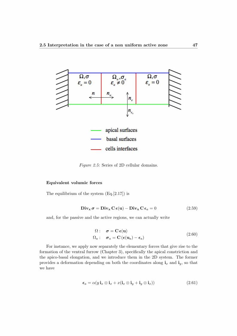
2.5 Interpretation in the case of a non uniform active zone 47
Figure 2.5: Series of 2D cellular domains.
Equivalent volumic forces
The equilibrium of the system (Eq.[2.17]) is
Divx ! = Divx C #(u)!Divx C #a = 0 (2.59)
and, for the passive and the active regions, we can actually write
# : ! = C #(u)#a : !a = C (#(ua)! #a)
(2.60)
For instance, we apply now separately the elementary forces that give rise to theformation of the ventral furrow (Chapter 3), specifically the apical constriction andthe apico-basal elongation, and we introduce them in the 2D system. The formerprovides a deformation depending on both the coordinates along ix and iy, so thatwe have
#a = "(y ix " ix + x(ix " iy + iy " ix)) (2.61)

48 Chapter 2. The kinematic model
where " is the deformation amplitude. Thus Divx!a is not constant, contraryto the case of the uniform extension along the apico-basal axis, since we find
#a = " iy " iy (2.62)
Therefore, in cartesian coordinates, even if cell interface forces are observed, weobtain volumic forces only when an apical constriction is applied. A more complexanalysis would be required instead for the specific case of the curvilinear coordinatessystem adopted to describe the embryo geometry.
Equivalent surface forces at cell interfaces
We are interested now in evaluating the e!ects that the active forces have alongthe cell interfaces. The mechanical equilibrium imposes that:
! (n) + !a (na) = 0 (2.63)
where n and na are the outward positive normals for the passive and the activedomains respectively (Fig. 2.5). If we introduce the relative expressions for ! and!a, we obtain
[C #(u)]n + [C #(ua)! #a]na = 0 (2.64)
so that
C[#(u)! #(ua)]n = C #a na '= 0 (2.65)
Thus the active forces can be replaced by surface forces along the interfaces be-tween the cells that will provide the main modes of deformation. For the specificcase of the mesoderm, which is modelled here as a continuum, the only interfacesare the ones between the active region, where the elementary deformations are in-troduced, and the passive zone. From a mechanical point of view, this means thatthe transition between the two regions plays a major role and could be the crucialsite where the tissues deformation is actually triggered. However we do not knowexactly if it is spread out across several cells, one cell or the interface between twocells.
In our formulation, the active region is defined by a Heaviside function, a unitstep function with a C1 derivative without overshoot whose value is 0 for a nega-tive argument and 1 for a positive one. The transition between these two values issmoothed within an interval which is user defined and could therefore represent the

2.5 Interpretation in the case of a non uniform active zone 49
Figure 2.6: Example of Heaviside functions on a cercle where an active and a passiveregions are defined. The transition between the two zones is determinedby an interval which is user defined; the higher the interval, the greaterthe smoothing e!ect.
key aspect of the problem (Fig. 2.6).
Equivalent surface forces at external cell boundaries
As similarly as for the internal interfaces, we can write the equilibrium along theexternal surfaces of each cell, thus we have
!a (nea) = fs (ne) (2.66)
where nea and ne are the outward positive normals to the active and the passivedomains respectively (Fig. 2.5); fs corresponds to the surface forces that are assumedhere equal to 0, while in the real Drosophila embryo they will be the yolk pressureon the internal surface of the mesoderm and the contact with the semi-rigid vitellinemembrane. If we recall the expression for !a, the previous equation becomes
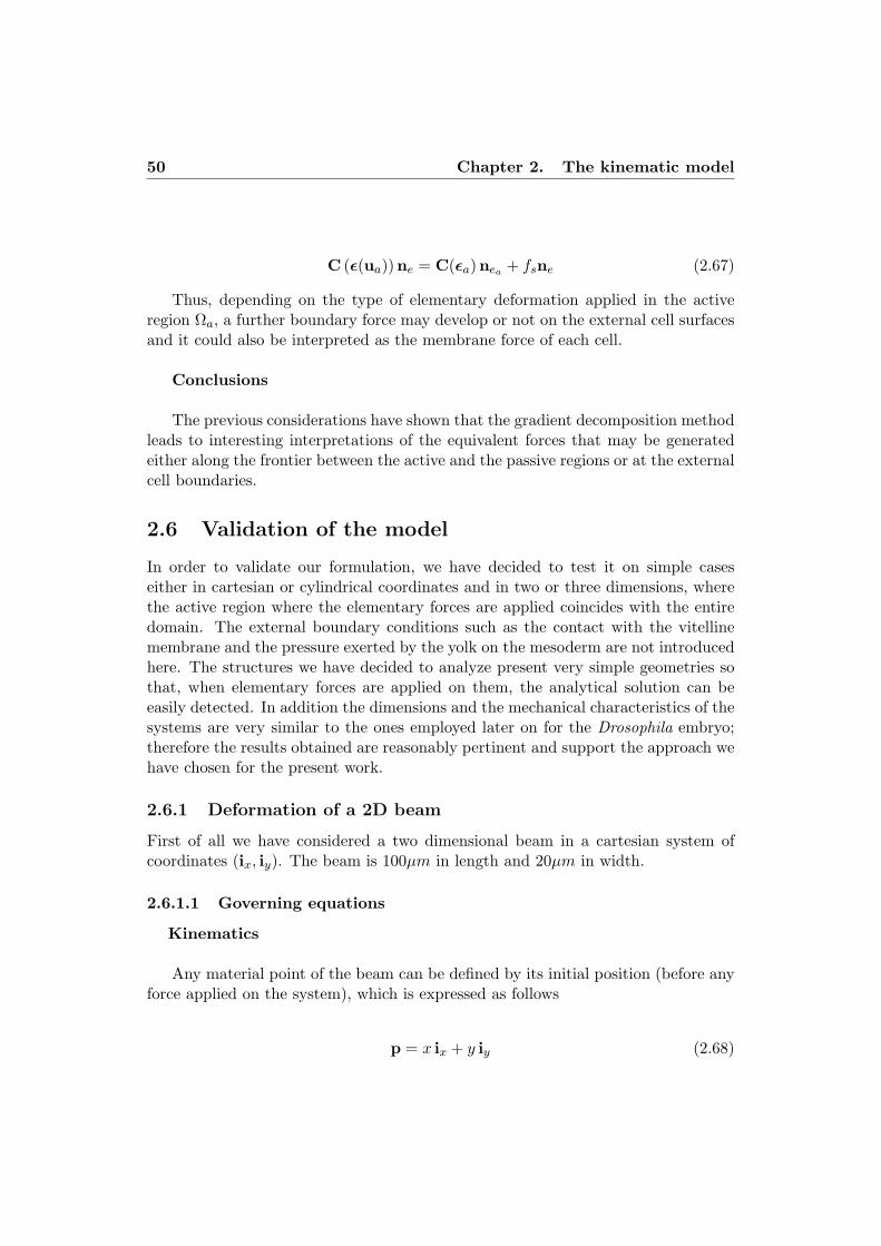
50 Chapter 2. The kinematic model
C (#(ua))ne = C(#a)nea + fsne (2.67)
Thus, depending on the type of elementary deformation applied in the activeregion #a, a further boundary force may develop or not on the external cell surfacesand it could also be interpreted as the membrane force of each cell.
Conclusions
The previous considerations have shown that the gradient decomposition methodleads to interesting interpretations of the equivalent forces that may be generatedeither along the frontier between the active and the passive regions or at the externalcell boundaries.
2.6 Validation of the model
In order to validate our formulation, we have decided to test it on simple caseseither in cartesian or cylindrical coordinates and in two or three dimensions, wherethe active region where the elementary forces are applied coincides with the entiredomain. The external boundary conditions such as the contact with the vitellinemembrane and the pressure exerted by the yolk on the mesoderm are not introducedhere. The structures we have decided to analyze present very simple geometries sothat, when elementary forces are applied on them, the analytical solution can beeasily detected. In addition the dimensions and the mechanical characteristics of thesystems are very similar to the ones employed later on for the Drosophila embryo;therefore the results obtained are reasonably pertinent and support the approach wehave chosen for the present work.
2.6.1 Deformation of a 2D beam
First of all we have considered a two dimensional beam in a cartesian system ofcoordinates (ix, iy). The beam is 100µm in length and 20µm in width.
2.6.1.1 Governing equations
Kinematics
Any material point of the beam can be defined by its initial position (before anyforce applied on the system), which is expressed as follows
p = x ix + y iy (2.68)

2.6 Validation of the model 51
Let us introduce a longitudinal extension, which can be considered as an activeelementary force on the system. Therefore each particle of the domain deforms toreach the intermediate position x equal to
x = (x + u) ix + (y + v) iy (2.69)
with u = "(t)x and v = 0. The deformation amplitude "(t) = " · t, with" = 0.05, depends on an incremental parameter t, which runs from 0 to 1, so thatthe final maximal deformation of the beam is obtained when "(t) = ".
Constitutive relations
We use a Saint-Venant material to describe the beam, as already presented inSec. 2.3, whose constitutive law is defined in Eq.[2.35]. The Young’s modulus E isfixed at 100Pa (as the one adopted for the embryo (Wiebe and Brodland [2005])) andthe Poisson’s coe"cient ) is equal to 0.45; thus the Lame’s coe"cients are obtainedfrom Eq.[2.37]. The values exploited for this specific case are the same employed forthe following examples presented in the next sections.
Equilibrium
No external forces are considered here, therefore the equilibrium equation takesinto account only the internal loads of the system and Eq.[2.28] becomes
&
!m
Tr("DpwT ) = 0 (2.70)
Boundary conditions
The boundary conditions play here an important role and highly a!ect the globalresponse of the structure, as already analyzed in Sec. 2.1 for the case of a single cell.We have considered three di!erent cases:
1. a simply supported beam on the lower boundary where v = 0 (Fig. 2.7a);
2. a cantilver beam on the left side where u = v = 0 and simply supported at thebottom (Fig. 2.7b);
3. a cantilever beam on both sides, u = v = 0, and simply supported again atthe bottom (Fig. 2.7c).

52 Chapter 2. The kinematic model
Figure 2.7: (a) Free beam (b) One side cantilever beam (c) Two sides cantileverbeam.
2.6.1.2 Solution
The active deformation gradient Fa can be deduced by Eq.[2.4] and we find
Fa = Dpx = [1 + "(t)] ix " ix + iy " iy (2.71)
The first case corresponds to a free dilatation; each element of the domain un-dergoes the elementary active deformation applied and changes its shape: thereforethe elastic passive deformation Fm (Eq. [2.2]) is equal to I so that F = Fa. Theextension is symmetric with respect to the vertical axis of the beam; the maxi-mal horizontal displacement for the left and right boundaries has been analyticallyfound, by the expression of the intermediate position x, at "(t) = " and is equalto (= ±2.5µm (Fig. 2.8a). The second and the third cases instead represent an ex-ample of impeded dilatation; when deformed by Fa, the individual cells are not freeto move because of the boundary conditions, therefore Fm '= I; thus the maximaldisplacements are the composition of the active and the passive contributions (Figs.
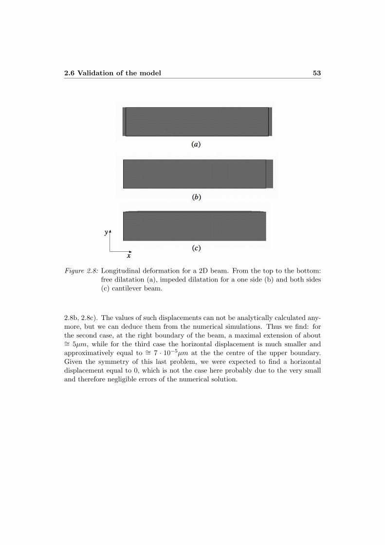
2.6 Validation of the model 53
Figure 2.8: Longitudinal deformation for a 2D beam. From the top to the bottom:free dilatation (a), impeded dilatation for a one side (b) and both sides(c) cantilever beam.
2.8b, 2.8c). The values of such displacements can not be analytically calculated any-more, but we can deduce them from the numerical simulations. Thus we find: forthe second case, at the right boundary of the beam, a maximal extension of about(= 5µm, while for the third case the horizontal displacement is much smaller andapproximatively equal to (= 7 · 10"5µm at the the centre of the upper boundary.Given the symmetry of this last problem, we were expected to find a horizontaldisplacement equal to 0, which is not the case here probably due to the very smalland therefore negligible errors of the numerical solution.

54 Chapter 2. The kinematic model
2.6.2 Deformation of a 3D beam
We consider now a three dimensional beam, with same length and width as beforeand thickness equal to 3µm.
2.6.2.1 Governing equations
Kinematics
As similarly as for the two dimensional case, in a three dimensional space (ix, iy, iz),the reference position for a generic point p of the beam is expressed as
p = x ix + y iy + z iz (2.72)
If we apply again an extension in the ix direction, the intermediate position xcan be written as
x = (x + u) ix + (y + v) iy + (z + w) iz (2.73)
where u = "(t) x , v = w = 0 and "(t) represents again the amplitude for thelongitudinal extension and t the incremental parameter, which runs from 0 to 1;the maximal dilatations for each case, whose values are the same as in the previoussection, have been found at "(t) = ", " equal to 0.05. The mechanical characteris-tics of the three dimensional beam are the same as for the two dimensional one; assimilarly as for the equation of the final equilibrium of the system.
2.6.2.2 Solution
The active deformation gradient Fa is equal to
Fa = Dpx = [1 + "(t)]ix " ix + iy " iy + iz " iz (2.74)
We have observed the influence of the boundary conditions on the final resultsand thus three di!erent cases have been considered as for the two dimensional case(Fig. 2.9). For what concerns the contributions of the active and the passive defor-mation, the considerations made in the previous section are still valid, therefore thevalues of the maximal displacements are the same found above (Sec. 2.6.1).
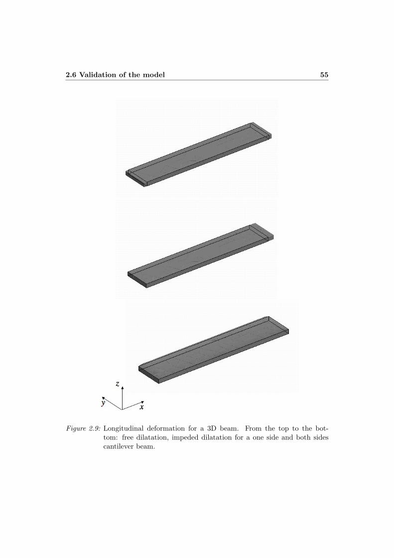
2.6 Validation of the model 55
Figure 2.9: Longitudinal deformation for a 3D beam. From the top to the bot-tom: free dilatation, impeded dilatation for a one side and both sidescantilever beam.

56 Chapter 2. The kinematic model
2.6.3 Radial and circular deformation of a circular cylinder section
Consider now a cross-section of a hollow circular cylinder in a cylindrical polarsystem of coordinates (r, +, z), with radius r =
/x2 + y2. The external and the
internal radius are respectively re = 50µm and ri = 45µm (Fig. 2.10).
Figure 2.10: Cross section of a hollow cylinder.
2.6.3.1 Governing equations
Kinematics
A generic point p can be located at its initial position by
p = r ir(+) (2.75)
where + = arctg" y
x
#. We have introduced two di!erent elementary forces: a
radial dilatation and a circular deformation. For the first case, the intermediateposition x can be written as follows
xrad = [1 + "(t)] r ir(+) (2.76)
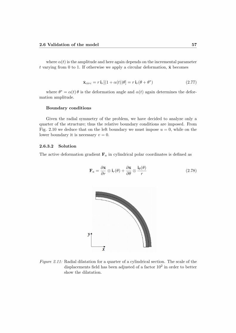
2.6 Validation of the model 57
where "(t) is the amplitude and here again depends on the incremental parametert varying from 0 to 1. If otherwise we apply a circular deformation, x becomes
xcirc = r ir[(1 + "(t))+] = r ir(+ + +#) (2.77)
where +# = "(t) + is the deformation angle and "(t) again determines the defor-mation amplitude.
Boundary conditions
Given the radial symmetry of the problem, we have decided to analyze only aquarter of the structure; thus the relative boundary conditions are imposed. FromFig. 2.10 we deduce that on the left boundary we must impose u = 0, while on thelower boundary it is necessary v = 0.
2.6.3.2 Solution
The active deformation gradient Fa in cylindrical polar coordinates is defined as
Fa =%x%r" ir(+) +
%x%+" i$(+)
r(2.78)
Figure 2.11: Radial dilatation for a quarter of a cylindrical section. The scale of thedisplacements field has been adjusted of a factor 102 in order to bettershow the dilatation.
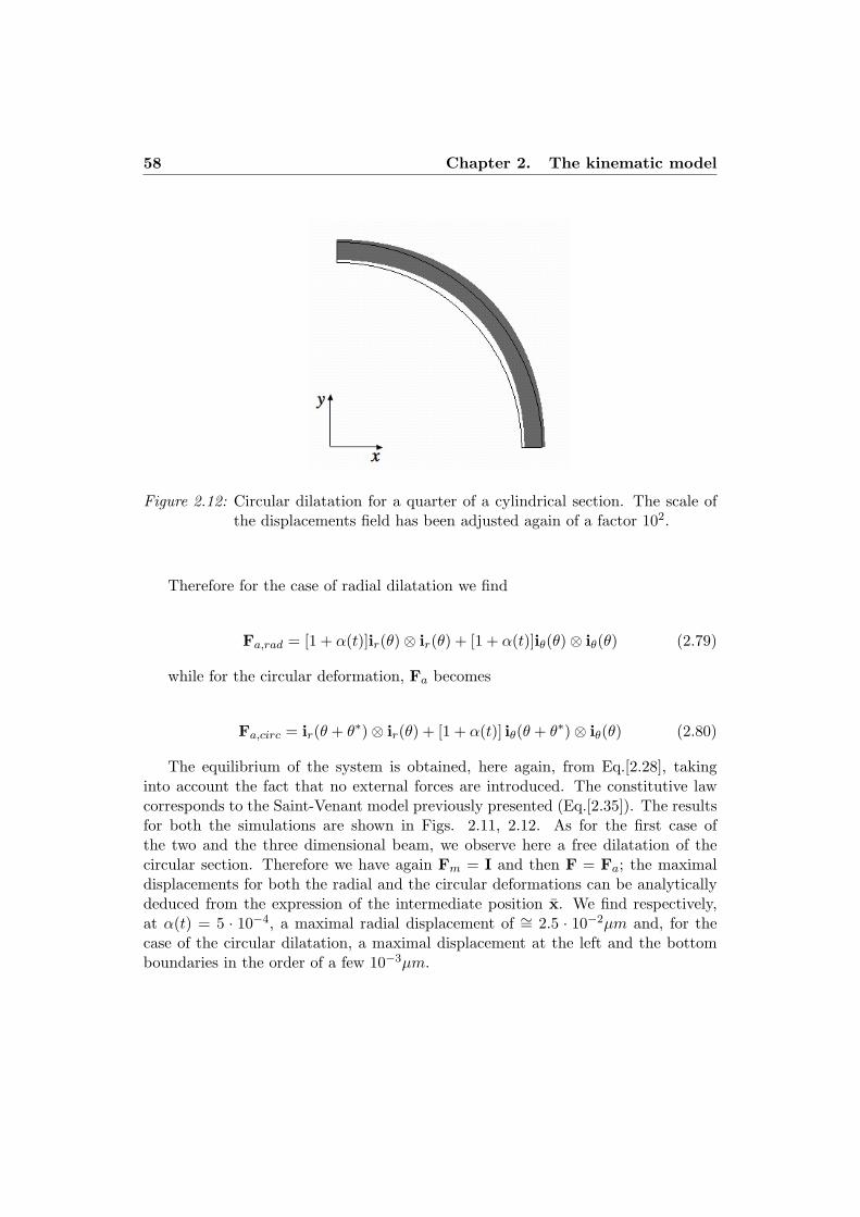
58 Chapter 2. The kinematic model
Figure 2.12: Circular dilatation for a quarter of a cylindrical section. The scale ofthe displacements field has been adjusted again of a factor 102.
Therefore for the case of radial dilatation we find
Fa,rad = [1 + "(t)]ir(+)" ir(+) + [1 + "(t)]i$(+)" i$(+) (2.79)
while for the circular deformation, Fa becomes
Fa,circ = ir(+ + +#)" ir(+) + [1 + "(t)] i$(+ + +#)" i$(+) (2.80)
The equilibrium of the system is obtained, here again, from Eq.[2.28], takinginto account the fact that no external forces are introduced. The constitutive lawcorresponds to the Saint-Venant model previously presented (Eq.[2.35]). The resultsfor both the simulations are shown in Figs. 2.11, 2.12. As for the first case ofthe two and the three dimensional beam, we observe here a free dilatation of thecircular section. Therefore we have again Fm = I and then F = Fa; the maximaldisplacements for both the radial and the circular deformations can be analyticallydeduced from the expression of the intermediate position x. We find respectively,at "(t) = 5 · 10"4, a maximal radial displacement of (= 2.5 · 10"2µm and, for thecase of the circular dilatation, a maximal displacement at the left and the bottomboundaries in the order of a few 10"3µm.

2.6 Validation of the model 59
2.6.4 Radial and circular deformation of a sphere
Among the 3D cases, it is interesting to analyze a sphere whose geometry is simpleand regular but more similar to the embryo than the previous examples studied;due to the symmetry of the problem, we only considered a eight of the sphere. Thesphere is defined in a spherical system of coordinates (r, +,,). The radius is equalto r =
/x2 + y2 + z2 with re = 100µm and ri = 95µm (Fig. 2.13).
Figure 2.13: Geometry of a sphere.
2.6.4.1 Governing equations
Kinematics
If we consider a material point of the sphere, its reference configuration is deter-mined by
p = r ir(+,,) (2.81)
where here again + = arctg"
zx
#. As for the circular cylinder, we impose first
a radial dilatation and then a circular deformation. Therefore the intermediateposition x is, for the first case, expressed as
xrad = [1 + "(t)]r ir(+,,) (2.82)
In the second case we find instead
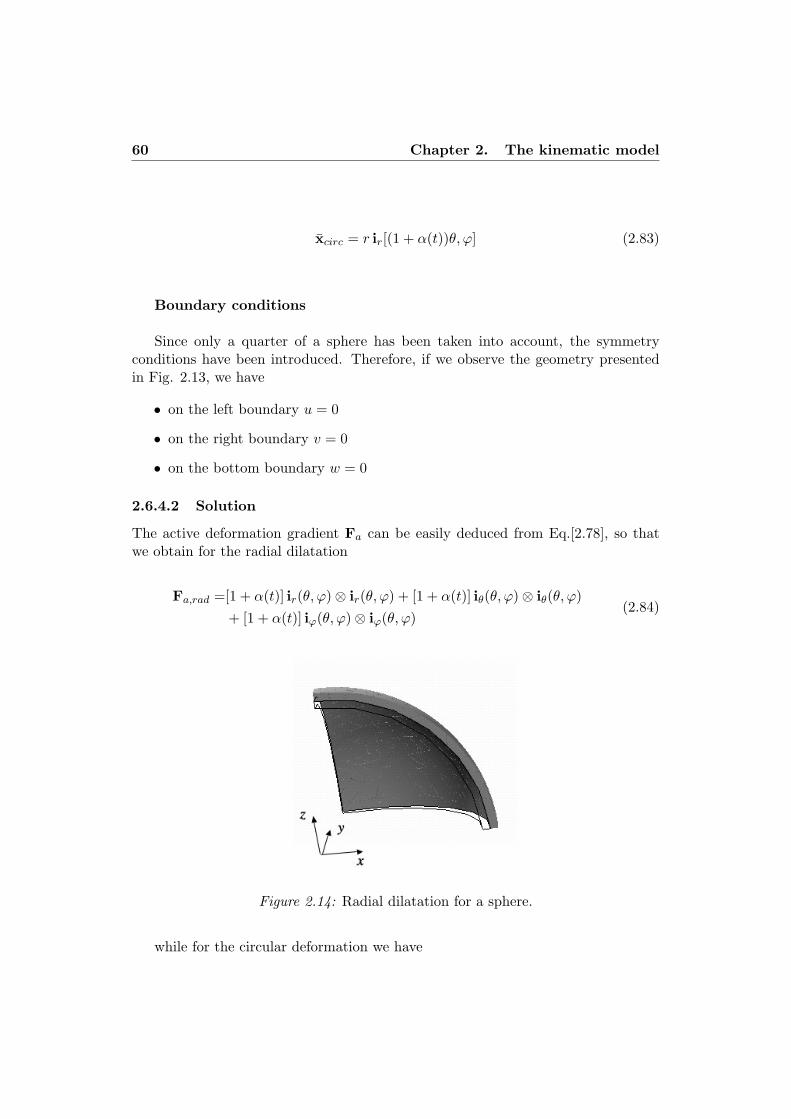
60 Chapter 2. The kinematic model
xcirc = r ir[(1 + "(t))+,,] (2.83)
Boundary conditions
Since only a quarter of a sphere has been taken into account, the symmetryconditions have been introduced. Therefore, if we observe the geometry presentedin Fig. 2.13, we have
• on the left boundary u = 0
• on the right boundary v = 0
• on the bottom boundary w = 0
2.6.4.2 Solution
The active deformation gradient Fa can be easily deduced from Eq.[2.78], so thatwe obtain for the radial dilatation
Fa,rad =[1 + "(t)] ir(+,,)" ir(+,,) + [1 + "(t)] i$(+,,)" i$(+,,)+ [1 + "(t)] i%(+,,)" i%(+, ,)
(2.84)
Figure 2.14: Radial dilatation for a sphere.
while for the circular deformation we have
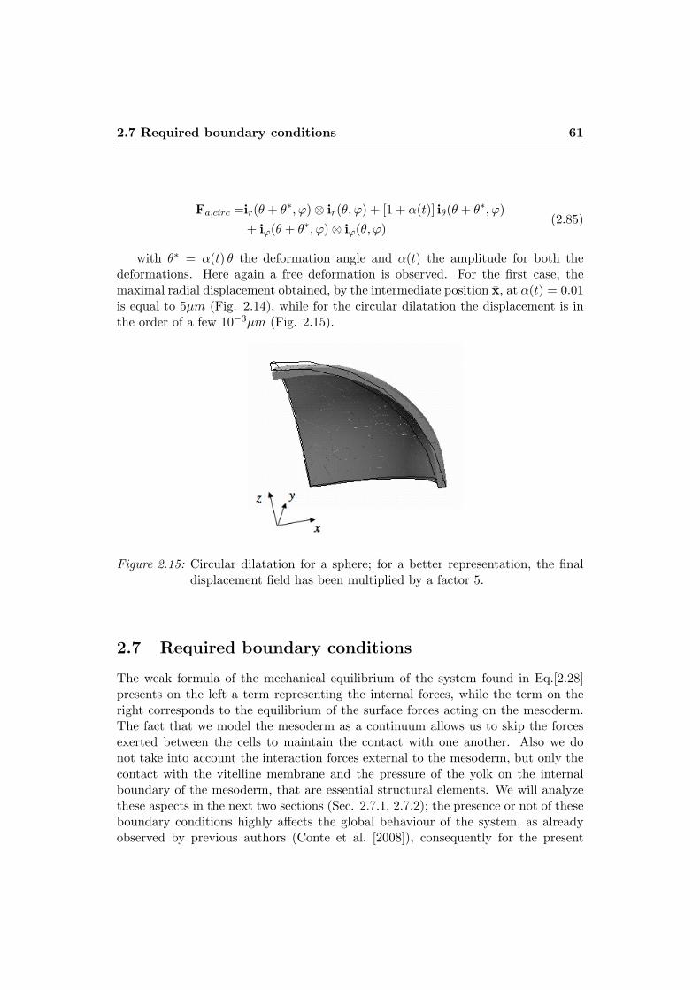
2.7 Required boundary conditions 61
Fa,circ =ir(+ + +#, ,)" ir(+,,) + [1 + "(t)] i$(+ + +#, ,)+ i%(+ + +#, ,)" i%(+,,)
(2.85)
with +# = "(t) + the deformation angle and "(t) the amplitude for both thedeformations. Here again a free deformation is observed. For the first case, themaximal radial displacement obtained, by the intermediate position x, at "(t) = 0.01is equal to 5µm (Fig. 2.14), while for the circular dilatation the displacement is inthe order of a few 10"3µm (Fig. 2.15).
Figure 2.15: Circular dilatation for a sphere; for a better representation, the finaldisplacement field has been multiplied by a factor 5.
2.7 Required boundary conditions
The weak formula of the mechanical equilibrium of the system found in Eq.[2.28]presents on the left a term representing the internal forces, while the term on theright corresponds to the equilibrium of the surface forces acting on the mesoderm.The fact that we model the mesoderm as a continuum allows us to skip the forcesexerted between the cells to maintain the contact with one another. Also we donot take into account the interaction forces external to the mesoderm, but only thecontact with the vitelline membrane and the pressure of the yolk on the internalboundary of the mesoderm, that are essential structural elements. We will analyzethese aspects in the next two sections (Sec. 2.7.1, 2.7.2); the presence or not of theseboundary conditions highly a!ects the global behaviour of the system, as alreadyobserved by previous authors (Conte et al. [2008]), consequently for the present
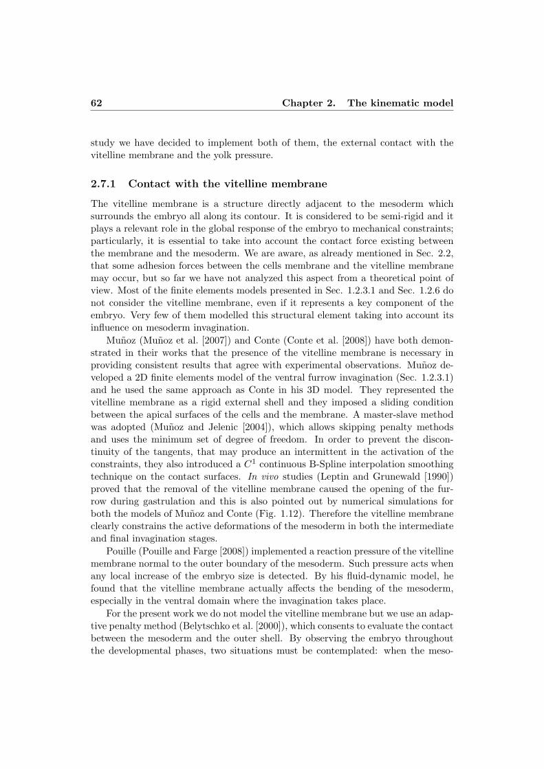
62 Chapter 2. The kinematic model
study we have decided to implement both of them, the external contact with thevitelline membrane and the yolk pressure.
2.7.1 Contact with the vitelline membrane
The vitelline membrane is a structure directly adjacent to the mesoderm whichsurrounds the embryo all along its contour. It is considered to be semi-rigid and itplays a relevant role in the global response of the embryo to mechanical constraints;particularly, it is essential to take into account the contact force existing betweenthe membrane and the mesoderm. We are aware, as already mentioned in Sec. 2.2,that some adhesion forces between the cells membrane and the vitelline membranemay occur, but so far we have not analyzed this aspect from a theoretical point ofview. Most of the finite elements models presented in Sec. 1.2.3.1 and Sec. 1.2.6 donot consider the vitelline membrane, even if it represents a key component of theembryo. Very few of them modelled this structural element taking into account itsinfluence on mesoderm invagination.
Munoz (Munoz et al. [2007]) and Conte (Conte et al. [2008]) have both demon-strated in their works that the presence of the vitelline membrane is necessary inproviding consistent results that agree with experimental observations. Munoz de-veloped a 2D finite elements model of the ventral furrow invagination (Sec. 1.2.3.1)and he used the same approach as Conte in his 3D model. They represented thevitelline membrane as a rigid external shell and they imposed a sliding conditionbetween the apical surfaces of the cells and the membrane. A master-slave methodwas adopted (Munoz and Jelenic [2004]), which allows skipping penalty methodsand uses the minimum set of degree of freedom. In order to prevent the discon-tinuity of the tangents, that may produce an intermittent in the activation of theconstraints, they also introduced a C1 continuous B-Spline interpolation smoothingtechnique on the contact surfaces. In vivo studies (Leptin and Grunewald [1990])proved that the removal of the vitelline membrane caused the opening of the fur-row during gastrulation and this is also pointed out by numerical simulations forboth the models of Munoz and Conte (Fig. 1.12). Therefore the vitelline membraneclearly constrains the active deformations of the mesoderm in both the intermediateand final invagination stages.
Pouille (Pouille and Farge [2008]) implemented a reaction pressure of the vitellinemembrane normal to the outer boundary of the mesoderm. Such pressure acts whenany local increase of the embryo size is detected. By his fluid-dynamic model, hefound that the vitelline membrane actually a!ects the bending of the mesoderm,especially in the ventral domain where the invagination takes place.
For the present work we do not model the vitelline membrane but we use an adap-tive penalty method (Belytschko et al. [2000]), which consents to evaluate the contactbetween the mesoderm and the outer shell. By observing the embryo throughoutthe developmental phases, two situations must be contemplated: when the meso-

2.7 Required boundary conditions 63
derm invaginates the yolk and when it evaginates exceeding the external boundary(Fig. 2.16). This last situation is forbidden by the assumption of the rigidity of thevitelline membrane.
Figure 2.16: Geometrical description of invagination and evagination of the meso-derm.
To deal with these cases, we want to check the contact constraint with thevitelline membrane %#e, which is defined by the equation
fc(xv) = 0 )xv (2.86)
where xv are the points on the vitelline membrane.We evaluate the distance, at the deformed configuration, between a point x on
the external surface of the mesoderm %#mexand its projection xv0 on the vitelline
membrane. The distance is calculated along the outward positive normal ncx to theexternal boundary of the mesoderm. Therefore we can write

64 Chapter 2. The kinematic model
fc(xv0) * fc(x) + (#fc(x),xv0 ! x) + · · · = 0 (2.87)
from which, in order to evaluate the repulsive forces, we deduce, at first order,the projection xv0 on the vitelline membrane of the point x
xv0 ! x = sc#fc(x) (2.88)
Thus sc represents the distance we are interested in and can be expressed as
sc(u) =!fc(p + u)
|#fc(p + u)|2 (2.89)
where the gradient of fc is evaluated as follows
#fc ÷ ncx =F"T (nc)+F"T (nc)+
(2.90)
fc acts as level set function (Osher and Fedkiw [2003], Sethian [1996]), so that0
fc(x) > 0 sc < 0fc(x) < 0 sc > 0
(2.91)
When writing the Principle of the Virtual Power, we need to know the expressionof the boundary force at the reference configuration. By Eq.[2.28] the right handside term for the specific case of the external contact with the vitelline membranebecomes
&
"!m
(w, fsJ F"T (n))dS =&
"!me
(w, pc(sc)J F"T (nc))dS (2.92)
where pc(sc) is the real pressure applied.As already said, the major issue comes when sc < 0 and the mesoderm evaginates
beyond its boundary. It is necessary in that case to apply a pushing-back force, while,when invagination occurs, we can easily control it by introducing a small constantforce. Thus we can write
0sc < 0 pc = !tc e(kcsc)/(tc)
sc > 0 pc = tc(2.93)
where tc and kc are constants whose values will be discussed in the next section.
2.7 Required boundary conditions 65
2.7.1.1 Circular dilation of a sphere when the external contact is intro-duced
To show the important role played by the vitelline membrane, we take back nowthe case of the sphere previously analyzed (Sec. 2.6.4) and we apply on the externalboundary of the domain the contact force. The values of the constant force tc andof kc have been chosen for this particular example and they will be the same forthe next simulations. tc is interpreted here as the adhesion force between the apicalsurface of a single cell and the vitelline membrane. It has been set at 1Pa and canbe compared to the traction force exerted by the cytoskeleton on the substrate towhich the cells naturally attach. Such force is concentrated at the focal adhesionsand it has been estimated between 10 and 30µN (Nicolas et al. [2004]): the largerthe adhesion zone, the higher the traction force. For our case, we assume that thecontact force involves the entire apical surface; this justifies the greater value of tcwith respect to the experimental data. The value of kc has been fixed at 1 · 108 inorder to have a maximal mesoderm evagination equal to 0.01µm.
If we recall the example of the circular deformation of a sphere (Fig. 2.15), wenotice an inhibition of the displacements compared to the cases where the externalcontact is not taken into account. Such reduction in deformation is due to the factthat, when the elements dilate, they are pushed back by the repulsive force imposedat the contour.
2.7.2 Internal yolk pressure
The yolk is a viscous fluid filling the internal region of the embryo and exertinga pressure on the internal surface of the mesoderm. The presence of the yolk canactually inhibit the invagination of the mesoderm as it has been noticed throughseveral numerical simulations (Ramasubramanian and Taber [2006], Conte et al.[2008]). Therefore in the latest models in the literature it has been taken intoaccount as a required component in order to have consistent results. There is stillan open question whether the fluid is incompressible or presents a residual pressureat the onset of ventral furrow invagination. Conte (Conte et al. [2008]) implementedboth the constancy of the volume and the initial pressure of the yolk using a penaltymethod where the total elastic potential of the epithelium is coupled with an extrapotential depending on the initial and the final volumes of the fluid. This approachallows not to consider the yolk as a fluid, but it ensures at the same time theminimal variations in volume. The only drawback of the method lies in the choiceof the penalty parameter, which is function of the sti!ness of the embryo; in theirstudy Conte and co-authors found volume variations less than 3.5%.
Taber modelled the yolk for the analysis of shell problems (Ramasubramanianand Taber [2006], Taber [2007]); he introduced hydrostatic incompressible fluid ele-ments and, by an auxiliary weak constraint condition, the embryo cavity was main-
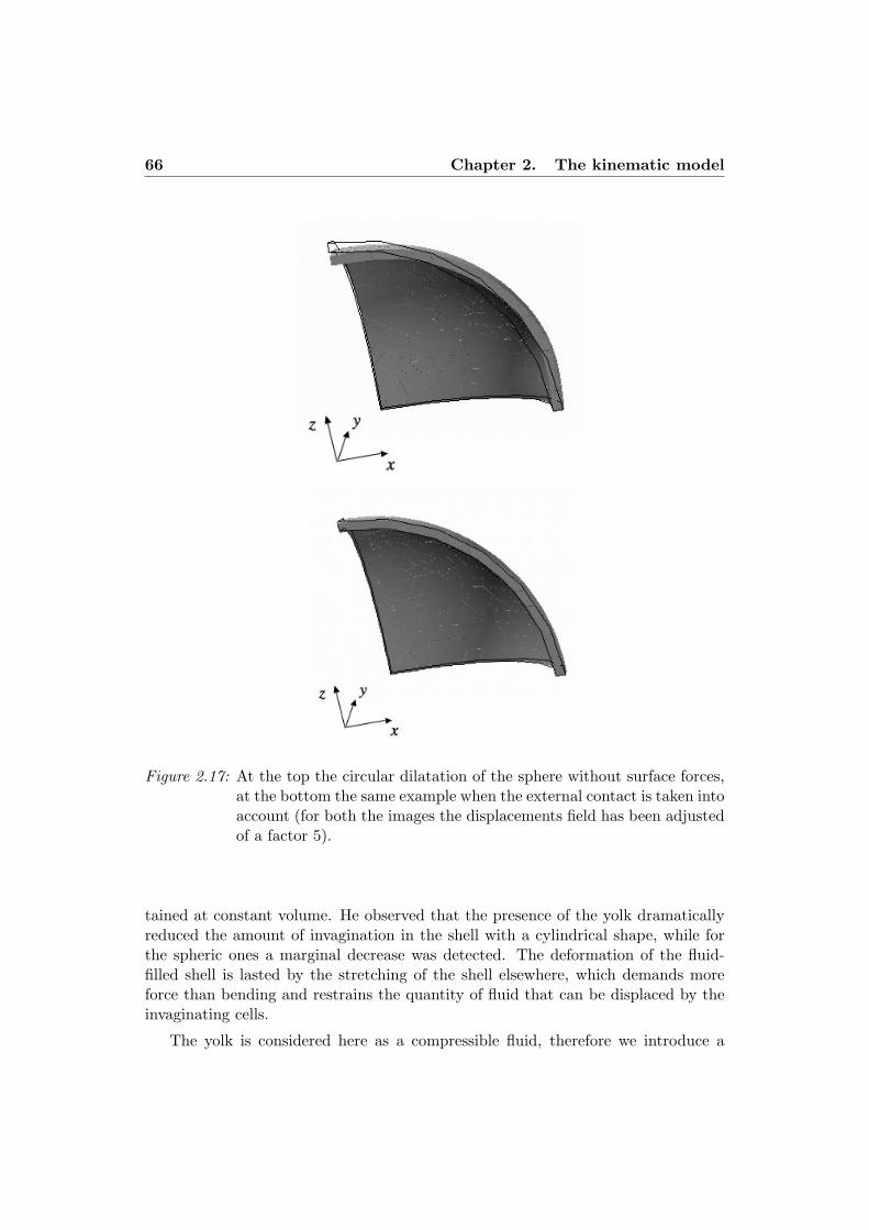
66 Chapter 2. The kinematic model
Figure 2.17: At the top the circular dilatation of the sphere without surface forces,at the bottom the same example when the external contact is taken intoaccount (for both the images the displacements field has been adjustedof a factor 5).
tained at constant volume. He observed that the presence of the yolk dramaticallyreduced the amount of invagination in the shell with a cylindrical shape, while forthe spheric ones a marginal decrease was detected. The deformation of the fluid-filled shell is lasted by the stretching of the shell elsewhere, which demands moreforce than bending and restrains the quantity of fluid that can be displaced by theinvaginating cells.
The yolk is considered here as a compressible fluid, therefore we introduce a

2.7 Required boundary conditions 67
uniform pressure py coupled with the global change of its volume. This method iscomputationally e"cient since we skip out the meshing of the yolk, thus we have adrastic decreasing of the number of degree of freedom.
We define the actual inner volume Vy, enclosed by the yolk, as
Vyx =&
!mix
dV (2.94)
Because of the Stoke’s formula, the previous equation can be rewritten as follows
Vyx =&
!mix
div x3
dVx =13
&
!mix
(x,nyx)dSx =13
&
"!mi
[x, J F"T (ny)] dS (2.95)
where nyx and ny are the positive inward normals to the internal boundary ofthe mesoderm at the deformed and undeformed configuration respectively.
Given the assumption of a fluid at rest, the applied pressure py(Vy), with Vy theinitial volume of the yolk, should satisfy the following pressure-volume law
py = py0 ! kyVyx ! Vy
Vy= py0 !
ky
Vy
&
"!m
(J F"1(p + u)! p,ny)dS (2.96)
where py0 and ky are respectively the initial pressure and the compressibilitycoe"cient of the yolk; in Sec. 3.4 we will discuss more in detail the choice of thesetwo constants. From the formulation of the Principle of the Virtual Power (Eq.[2.28]), we can write the second right hand side term as follows
&
"!mi
["(ny),w] dS =&
"!mi
[py(Vy)(ny),w] dS
=&
"!mi
py(Vy)[J F"T (ny),w]dS
=&
"!mi
py
113
&
"!mi
[xa, J F"T (nya)]dS
2[J F"T (nyb),w]dS
(2.97)
Thus there is a double integration: the first one to get the correct yolk pressure(indicated here by the subscript a) and the second one to get the virtual workon the internal boundary of the mesoderm (indicated here by the subscript b). Thenumerical issue related to this peculiar term will be discussed in the following section.

68 Chapter 2. The kinematic model
2.8 Iterative scheme and finite elements approximation
We recall here the weak formula of the mechanical equilibrium of the system, ob-tained in Sec. 2.2, which can be rewritten as follows
&
!m
Tr""(u, "i(t)),DpwT
#=
&
"!me
"pcJF"T (nc),w
#dS
+&
"!mi
"pyJF"T (ny),w
#dS
(2.98)
where the left hand side term represents the internal forces expressed by theFirst Piola-Kirchho! tensor ", which is function of the displacement u and of thedeformation amplitude "i(t) that will be later on defined and change according tothe morphogenetic movement considered. The right hand terms instead representrespectively the contact force between the mesoderm and the vitelline membrane andthe pressure force exerted by the yolk on the internal boundary of the mesoderm.Such expression is proposed here to describe the numerical method employed for thepresent work, which consists of an incremental implicit scheme through the evolutionparameter t, together with a Newton technique to solve the corresponding non linearproblem at each time step.
The time interval ]0, T [ is decomposed into tn steps, n = 1, N , and, starting fromusual vanishing initial values, the displacement un+1 is computed, so that we obtain
&
!m
Tr""(un+1, ("i(t))n+1),DpwT
#=
&
"!me
+"pcJF"T (nc)
#n+1,w
,dS
+&
"!mi
+"pyJF"T (ny)
#n+1,w
,dS
(2.99)
With respect to the space variable, the displacement vector is decomposed onthe classical finite element basis function with Lagrangian polynomial of degree twoon a thetrahedral mesh. The convergence criterion is based on the L2 norm of thedisplacement with a tolerance 10"2 on the relative error. The derivation of theNewton scheme is done in the following way: at iteration k + 1 and time step n + 1,the previous equilibrium equation is expanded with respect to un+1,k, thus we have

2.8 Iterative scheme and finite elements approximation 69
&
!m
Tr+"
-un+1,k, ("i(t))n+1
.,DpwT
,!
&
"!me
+"pcJF"T
#n+1,k (nc),w,dS
!&
"!mi
+"pyJF"T
#n+1,k (ny),w,dS
+&
!m
Tr+Du"
--un+1,k
.&un+1,k+1,
""i(t)
#n+1.
,DpwT,
!&
"!me
+Du
"pcJF"T
#n+1,k&un+1,k+1(nc),w
,dS
!&
"!mi
+Du
"pyJF"T
#n+1,k&un+1,k+1(ny),w
,dS = 0
(2.100)
so that the displacement increment &un+1,k+1 can be computed by the solutionof a linear system.
Yolk pressure and contact with the vitelline membrane
The yolk boundary condition presents a special issue because it is non local. Thisis mostly due to the fact that the yolk is assumed here to be a fluid at rest and thereis a relation between its global volume change and the uniform pressure appliedon the mesoderm, as shown in Eq.[2.96]. Therefore, as described in Eq.[2.97], weget a double integral: one provides the correct yolk pressure, the other the virtualwork on the internal boundary %#mi of the mesoderm. This leads to a Jacobianmatrix Du
"pyJF"T
#n+1,k where all the nodes at the boundary are coupled. Givenseveral di"culties related to the large computer memory required, we have decidedto compute the Jacobian one iteration behind in order to annihilate such complexcoupling between the nodes of the inner boundary. The computational cost is verymuch reduced with no noticeable degradation in the number of Newton iterationsuntil convergence. The di!erent examples that have been treated never showed anypathological di"culty inherited from this simplified choice. This is certainly due tothe fact that only average volume occurs in the expression of the pressure, which isconsequently not significantly oscillating.
For what concerns the contact with the external vitelline membrane, we stillhave to consider it as a non linear boundary condition, but, contrary to the yolk, itis locally defined.

70 Chapter 2. The kinematic model
2.9 Hints for a future stability analysis
The convergence of the previous Newton scheme crucially depends on the Jacobian ofthe First Piola-Kirchho! tensor with respect to the displacement. In this paragraph,we try to evaluate this quantity through an incremental analysis.
The derivative term Du""u, "i(t)
#, as similarly as
"Du pcJ F"T
#for the contact
force and"Du pyJ F"T
#for the yolk pressure, can be obtained from the following
rate type equation
d"
dt= Du"
dudt
+ D&i"d"i(t)
dt(2.101)
where t is the incremental parameter, which determines the amplitude "i(t) (seeChapter 3), and u is the displacement. Since " = FS, the term on the left handcan actually be expressed as
d"
dt=
dFdt
S + FdSdt
(2.102)
with F, the final deformation gradient, equal to F = I+Dpu, so that its deriva-tive becomes
dFdt
= Dp
$dudt
%(2.103)
The Second Piola-Kirchho! tensor S can be formulated here as in Eq.[2.54], thuswe obtain
dSdt
=dCFa
dt: (E!Ea) + CFa :
$dEdt! dEa
dt
%(2.104)
Then Eq.[2.102] can be rewritten as
d"
dt= Dp
$dudt
% )CFa : (E!Ea)
*+ CFa : FTDp
$dudt
%
+ F'dCFa
dt: (E!Ea)!CFa :
dEa
dt
( (2.105)
This last equation expresses the dependency of " on both the gradient of thevelocity du
dt and the increment of the active deformations. The analysis of the tangentsti!ness appearing in the first and the second terms of the equation would give thepath to evaluate the stability of the highly non linear problem. Such aspect is notfurther elaborated for the present work, but it may be the object of future studies.
2.10 Conclusions 71
2.10 Conclusions
This section of the work has provided a general overview of the approach used for theanalysis of the specific morphogenetic movements that will be described in detailsin the next chapter.
A single cell naturally tends to deform because of chemical signals developingthrough the cytoskeleton. Such free deformation is not completely possible when thecell, with other cells, is part of a system and therefore constrained not only by itsneighbours but also by external boundary conditions. This is the case of the embryowhere the cells are in contact with one another and with the yolk and the vitellinemembrane on their basal and apical surfaces respectively. Therefore when the ele-mentary forces occur, the cells modify their shape, but a geometrical incompatibility(i.e. superposition of the volumes) is observed which does not guarantee the con-tinuity of the system; therefore the mesoderm reacts and the passive deformationtakes place.
The gradient decomposition method is very useful since it allows to take into ac-count both the active and the passive deformations that are strongly interconnectedand have to be composed to obtain the final and correct tissues deformation. Thenecessary abstract tools have been amply described in this chapter. In particular wehave focused on the computation of the active deformation gradient, which, in thecurvilinear coordinates system later on introduced, changes according to each mor-phogenetic movement considered and therefore to the elementary forces introduced.Also we have shown how, by the Principle of the Virtual Power, we express themechanical equilibrium of the system that includes both the forces at the interior ofthe domain and the boundary conditions, such as the yolk pressure and the vitellinemembrane. Actually these two components, even if not explicitly modelled here, areessential structural elements and the absence of one or both of them may lead tofinal configurations that do not correspond to experimental observations.
If from a mechanical point of view the gradient decomposition method is nat-ural and logic and often used for large deformations problems, biologists may beperplex in finding the physical meaning of such approach. Thus we have proposedsome interesting interpretations of the method that have pointed out novel aspectsso far unexplored and further hints of discussion. Specifically, we have presentedthe similarities between our formulation and the stress analysis in thermodynam-ics problems. This analysis better clarifies the composition of the active and thepassive deformations, which is here compared to the initial and final contributionsin thermal dilatation. Additionally, we have shown the local e!ects of the activeforces introduced in our formulation. First of all, we have concluded that they couldbe replaced by surface forces along the cells interfaces that would provide the maindeformation modes. For our specific case, it seems to us that the transition betweenthe active and the passive regions constitutes the crucial site where the deformationis actually triggered and it has therefore to be taken into account very carefully.

72 Chapter 2. The kinematic model
Secondly, we have noticed that, when introducing the active forces in the activedomain, we also collect a consequent strain at the internal and external boundaries,to include with the already present yolk pressure and the contact with the vitellinemembrane.
Another point on which biologists may not fully agree concerns the choice ofthe constitutive law of the mesoderm. For the present work we have opted for alinear Saint-Venant model that does not consider instead the non-linearities of thematerial provided by its visco-elastic traits and, additionally, it is in contrast with theprevious works where a Hyperelastic material has often been used. The main reasonfor this choice is the lack in information about the mechanical characteristics of themesoderm that are usually very di"cult to detect. Although we have comparedthe two models and we will show later that the results for both cases are not sodi!erent, which is also probably due to the very small deformations occurring tothe mesoderm. However we are aware that the Saint-Venant material presents somelimitations and therefore we are working on those aspects so far put aside. On theother hand it is evident that the analysis of a biological system is not always easyfor the many parameters that take part to the processes, thus the hypothesis made,even if simplistic at first sight, may still be useful for a qualitative analysis of theproblem.
Finally we have briefly presented the numerical method used to solve the nonlinear problem; it consists of an incremental implicit scheme together with a New-ton technique. Special caution has to be made for the implementation of the yolkpressure which is not local therefore treated here at a fixed point to avoid largecomputer memory. Additionally we have analyzed the stability of the solution in or-der to evaluate the critical values of the incremental parameter at which bifurcatione!ects may occur and thus a!ect the right properties of convergence.
In the next chapter we are going to focus on each morphogenetic movement.Specifically we will show how, from the analytical expression of the intermediateposition of a generic point, which changes according to the elementary forces applied,we obtain the equation corresponding to the active deformation gradients.

Chapter 3
Morphogenetic movements inDrosophila embryo
This section of the work is dedicated to the detailed description of the relative for-mulations for the three morphogenetic movements: the two furrows (ventral andcephalic) are presented together in Sec. 3.2, while the germ band extension in Sec.3.3. In particular, we show how we obtain, by the parametrical description of theembryo in a curvilinear system of coordinates (Sec. 3.1), the reference configura-tion of a material point and its intermediate position when the primary forces areintroduced. The active deformation gradients change according to the active de-formations and they are therefore user defined and proper to each morphogeneticmovement considered.
In the second part of the chapter we present the results obtained (Sec. 3.4),evaluating them for each simulation. For the ventral furrow, a parametric analysishas been conducted, pointing out the variables that may influence the final con-figuration, such as the size of the active region (Sec. 3.5.1), the dimensions of thematerial cells (Sec. 3.5.2) and the presence of the apico-basal elongation (Sec. 3.5.3).In Sec. 3.9 and 3.10 we propose an estimation of the induced pressures and shearstress that are engendered elsewhere than the active regions when the elementarydeformations are applied on the cells. This analysis in particular allows us to confirmnot only qualitatively, but also from a quantitative point of view, some hypothesesput forward by biologists.
As said in Sec. 1.3 and 2.1, we use an ellipsoid to model the embryo, which has tobe considered as an approximation of the real biological system. Actually in this waywe do not consider the di!erent curvature between the anterior and the posteriorpole, which may influence those movements occurring along the anterior-posterioraxis such as ventral furrow invagination and germ band extension. Therefore wehave performed an interesting collateral study, in collaboration with Anne-SophieMouronval of the MSSMat Laboratory, that consents to compare di!erent geometries
73
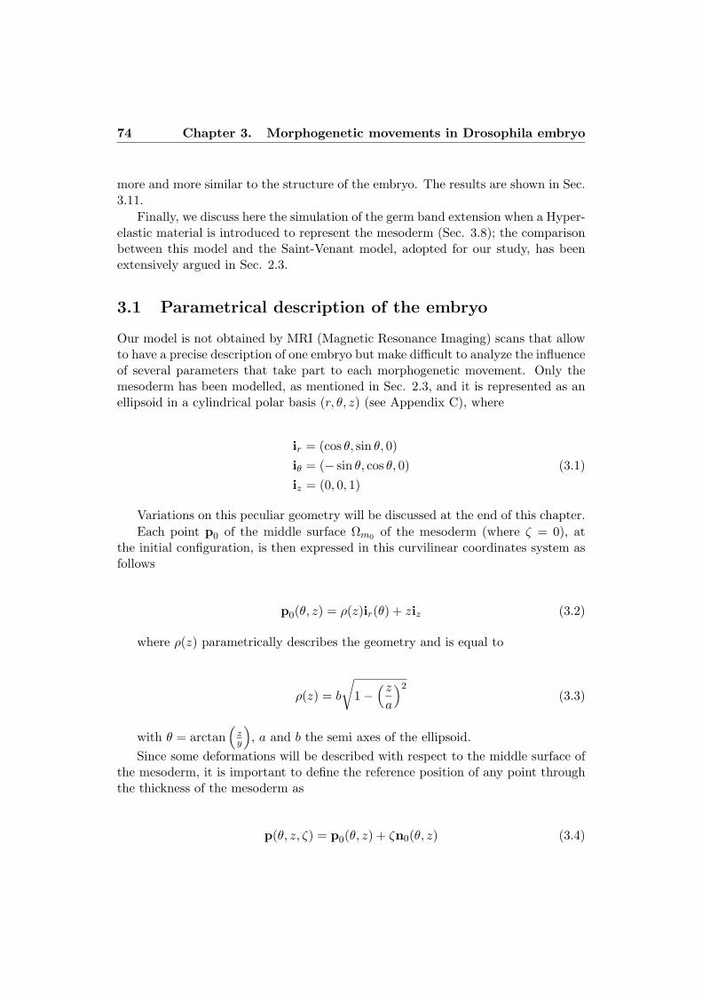
74 Chapter 3. Morphogenetic movements in Drosophila embryo
more and more similar to the structure of the embryo. The results are shown in Sec.3.11.
Finally, we discuss here the simulation of the germ band extension when a Hyper-elastic material is introduced to represent the mesoderm (Sec. 3.8); the comparisonbetween this model and the Saint-Venant model, adopted for our study, has beenextensively argued in Sec. 2.3.
3.1 Parametrical description of the embryo
Our model is not obtained by MRI (Magnetic Resonance Imaging) scans that allowto have a precise description of one embryo but make di"cult to analyze the influenceof several parameters that take part to each morphogenetic movement. Only themesoderm has been modelled, as mentioned in Sec. 2.3, and it is represented as anellipsoid in a cylindrical polar basis (r, +, z) (see Appendix C), where
ir = (cos +, sin +, 0)i$ = (! sin +, cos +, 0)iz = (0, 0, 1)
(3.1)
Variations on this peculiar geometry will be discussed at the end of this chapter.Each point p0 of the middle surface #m0 of the mesoderm (where $ = 0), at
the initial configuration, is then expressed in this curvilinear coordinates system asfollows
p0(+, z) = '(z)ir(+) + ziz (3.2)
where '(z) parametrically describes the geometry and is equal to
'(z) = b
31!
-z
a
.2(3.3)
with + = arctan-
zy
., a and b the semi axes of the ellipsoid.
Since some deformations will be described with respect to the middle surface ofthe mesoderm, it is important to define the reference position of any point throughthe thickness of the mesoderm as
p(+, z, $) = p0(+, z) + $n0(+, z) (3.4)
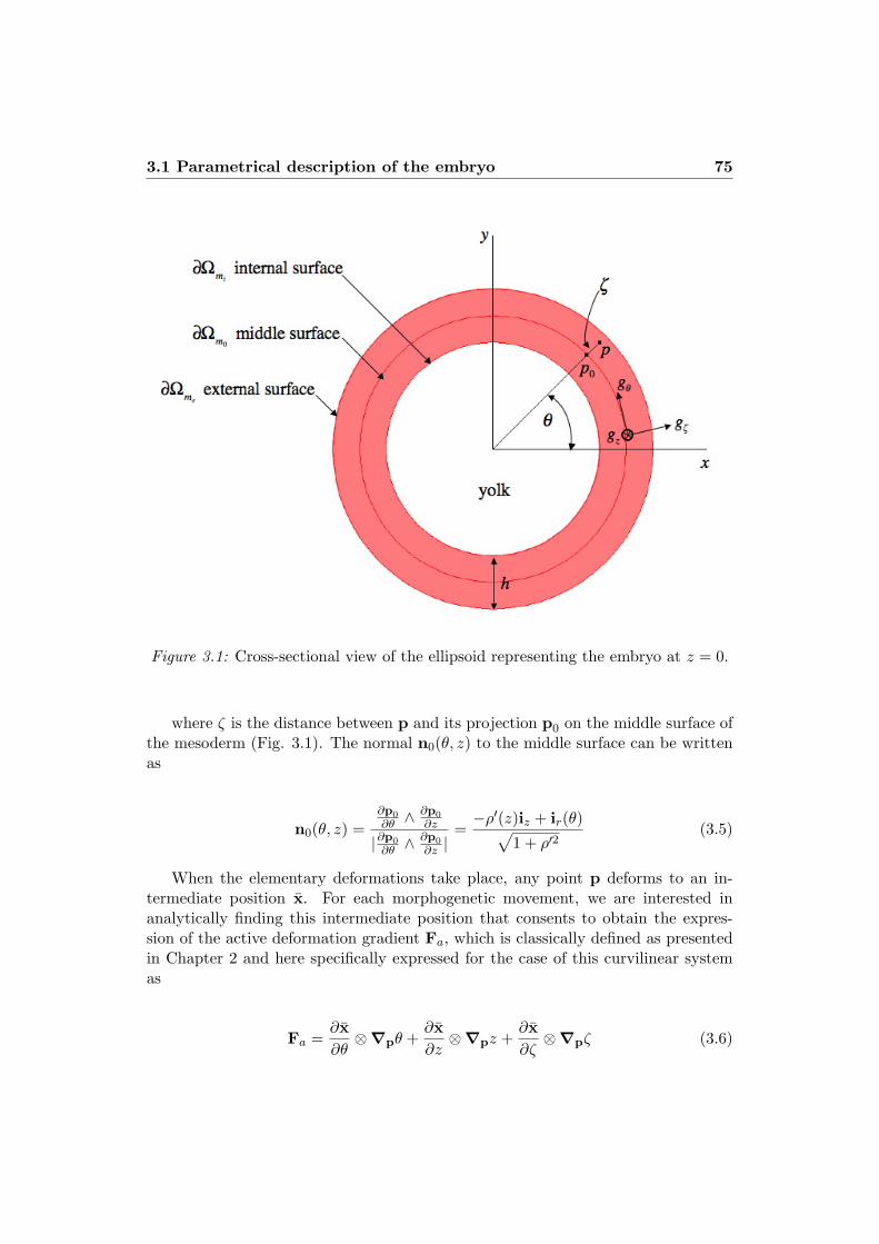
3.1 Parametrical description of the embryo 75
Figure 3.1: Cross-sectional view of the ellipsoid representing the embryo at z = 0.
where $ is the distance between p and its projection p0 on the middle surface ofthe mesoderm (Fig. 3.1). The normal n0(+, z) to the middle surface can be writtenas
n0(+, z) ="p0"$ $
"p0"z
|"p0"$ $
"p0"z |
=!'$(z)iz + ir(+)/
1 + '$2(3.5)
When the elementary deformations take place, any point p deforms to an in-termediate position x. For each morphogenetic movement, we are interested inanalytically finding this intermediate position that consents to obtain the expres-sion of the active deformation gradient Fa, which is classically defined as presentedin Chapter 2 and here specifically expressed for the case of this curvilinear systemas
Fa =%x%+"!p+ +
%x%z"!pz +
%x%$"!p$ (3.6)

76 Chapter 3. Morphogenetic movements in Drosophila embryo
where
!p+ =gz $ g'
g
!pz =g' $ g$
g
!p$ =g$ $ gz
g
(3.7)
form the contravariant basis in p (see Sec. 2.1) and g is defined as in Eq.[2.15].g$,gz,g' are instead the tangent vectors to the curve when $ '= 0 and they can
be calculated from Eq.[3.4] as
g$ =%p%+
=%p0
%++ $
%n0
%+
gz =%p%z
=%p0
%z+ $
%n0
%z
g' =%p%$
= n0(+, z)
(3.8)
If we develop Eq.[3.8], we find
g$ = ,$i$(+) (3.9)
gz = ,z('$(z)ir(+) + iz) (3.10)
g' =!'$(z)iz + ir(+)/
1 + '$2(z)(3.11)
where
,$ =
1'(z) +
$/1 + '$2(z)
2
,z =
11! $'$$(z)
(1 + '$2(z))3/2
2 (3.12)
Therefore g can be calculated as
g = ,$,z
/1 + '$2(z) (3.13)
If we substitute the expressions of the tangent vectors (Eq.[3.9, 3.10, 3.11]) inthe relative gradients (Eq.[3.7]), we obtain

3.2 Ventral furrow invagination and cephalic furrow formation 77
!p+ =i$(+),$
!pz ='$(z)ir(+) + iz,z(1 + '$2(z))
!p$ = n0(+, z)
(3.14)
The parametrical description of the geometry of the embryo is one of the majoradvantage of our model, since it allows having the precise analytical expressionsof the intermediate position x, which are therefore proper to each event and userdefined, given the dependence on the elementary forces introduced. The influence ofthe geometry will be discussed later on in this chapter; we are now going to analyzethe di!erent morphogenetic movements.
3.2 Ventral furrow invagination and cephalic furrow for-mation
Ventral furrow invagination and cephalic furrow formation take place simultane-ously during embryogenesis and are very similar since triggered by almost the samemechanical constraints. Both the morphogenetic movements can be considered asorthogonal invaginations of the mesoderm (Sec. 1.2.2); in fact invagination occursalong a line rather than at a single point. A trough forms (Fig. 1.2), the axis ofwhich is parallel to the original surface, thus at right angles with respect to thedirection of invagination (Davies [2005]).
Figure 3.2: Cross sections of the embryo showing the successive phases of ventralfurrow invagination (Leptin [1999]). The di!erent colours mark the re-gions or the cells where invagination occurs.
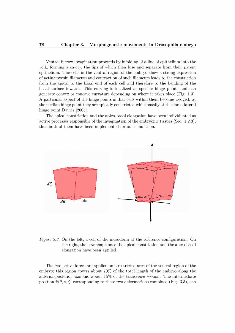
78 Chapter 3. Morphogenetic movements in Drosophila embryo
Ventral furrow invagination proceeds by infolding of a line of epithelium into theyolk, forming a cavity, the lips of which then fuse and separate from their parentepithelium. The cells in the ventral region of the embryo show a strong expressionof actin/myosin filaments and contraction of such filaments leads to the constrictionfrom the apical to the basal end of each cell and therefore to the bending of thebasal surface inward. This curving is localized at specific hinge points and cangenerate convex or concave curvature depending on where it takes place (Fig. 1.3).A particular aspect of the hinge points is that cells within them become wedged: atthe median hinge point they are apically constricted while basally at the dorso-lateralhinge point Davies [2005].
The apical constriction and the apico-basal elongation have been individuated asactive processes responsible of the invagination of the embryonic tissues (Sec. 1.2.3),thus both of them have been implemented for our simulation.
Figure 3.3: On the left, a cell of the mesoderm at the reference configuration. Onthe right, the new shape once the apical constriction and the apico-basalelongation have been applied.
The two active forces are applied on a restricted area of the ventral region of theembryo; this region covers about 70% of the total length of the embryo along theanterior-posterior axis and about 15% of the transverse section. The intermediateposition x(+, z, $) corresponding to these two deformations combined (Fig. 3.3), can

3.2 Ventral furrow invagination and cephalic furrow formation 79
be written as follows
x(+, z, $) = p0(+, z) +-1 + "abe(t)
.$n0(+, z) (3.15)
where "abe(t) is the amplitude of the apico-basal elongation and
+ = + + "ac(t)2$
hm(+) (3.16)
is the deformation angle depending on "ac(t), the amplitude of the apical con-striction; h is the thickness of the mesoderm (Fig. 3.1). m(+) is a periodic function,normalized between !1 and 1, that mimics the material cells themselves by whichthe deformation region is subdivided (Fig. 3.4).
Figure 3.4: The trend of the periodic function m(+) along a circular section. Itallows to have the same deformation along the section of the active regionwhere ventral furrow invagination takes place. For this specific imageand for sake of simplicity in the representation, the active region coversall the circular section, while for the case of the embryo it is restrainedto a smaller domain. The same function is used for the cephalic furrowsimulation (m(z)).

80 Chapter 3. Morphogenetic movements in Drosophila embryo
Such function is expressed as
m(+) = 2$
+
+cell! 1
2! round
$+
+cell! 1
2
%%(3.17)
with +cell corresponding to the dimensions of a material cell along the sectionof the embryo and round being the classical step function, which gives the integernumber of $
$cell. The introduction of this periodic function has been necessary in
order to have the same deformation around the mesoderm cross section where +increases.
The deformation amplitudes "abe(t) and "ac(t) are defined as
"abe(t) = "abe · t"ac(t) = "ac · t
(3.18)
with "abe and "ac constants that are adjusted in order to assure at the sametime the right properties of convergence and consistent final configurations. t is theevolution parameter, which varies between timin and tiMAX ; here the superscript iindicates the movement considered, since the minimal and the maximal values of tvary according to the simulated event.
Similar equations can be derived for the cephalic furrow, shaped by two parallelstrips of cells undergoing an inward flexion movement. Given the di!erent axis withrespect to which the invagination takes place, this time the active deformation occursalong the z direction (Fig. 3.5), therefore the intermediate position x(+, z, $) of ageneric point can be written as follows
x(+, z, $) = p0(+, z) + $ n0(+, z) (3.19)
with
z = z + "ceph(t)2$
hm(z) (3.20)
where "ceph(t) is the amplitude of the deformation (here only apical constrictionhas been introduced), defined as "ceph(t) = "ceph · t, with "ceph a suitable constant.m(z) is again a periodic function as defined in Eq.[3.17], depending this time on zet zcell , which represents the cell dimensions in the z direction.
Finally, Fia can be computed for both cases from Eq.[3.6] in the curvilinear
coordinates system fitted here for the ellipsoidal idealized geometry of the embryo.Thus we obtain respectively for the ventral furrow

3.2 Ventral furrow invagination and cephalic furrow formation 81
Figure 3.5: Apical constriction along the anterior-posterior axis for a cell during thecephalic furrow formation.
FV FIa =
+1 + "ac(t)2'
h m$(+),,V FI
$
,$i$(+)" i$(+)
+('$(z)ir(+) + iz),V FI
z
(1 + '$2(z)),z" ('$(z)ir(+) + iz)
+'2"ac(t)
hm(+),V FI
$ i$(+) + (1 + "abe(t))n0(+, z)(" n0(+, z)
(3.21)
where ,$ and ,z are the same as defined in Eq.[3.12], while
,$V FI =
4'(z) +
(1 + "abe(t))$/1 + '$2(z)
5
,zV FI =
'1! (1 + "abe(t))$ '$$(z)
(1 + '$2(z))3/2
( (3.22)
If we analyze the previous expressions we can notice that the term (1 + '$2(z))gives the curvilinear abscissa along the embryo. At the dorsal and ventral regionswe have '$(z) = 0, while at the anterior and posterior poles '$(z) = ,, therefore thedeformation determined by "i(t) is whether inhibited or sharpened. On the otherhand '$$(z) provides the curvature of the embryo which highly a!ects the apical

82 Chapter 3. Morphogenetic movements in Drosophila embryo
constriction. Actually the greater the curvature, the more evident the e!ects of theconstriction. Therefore it would be interesting to perform a sensibility analysis inorder to evaluate the influence of the curvature on the final configuration. Thisaspect has been partly argued by testing di!erent embryo geometries that take intoaccount some peculiar characteristics, as amply described in Sec. 3.11.
For the cephalic furrow the active deformation gradient FCFa is
FCFa =
,CF$
,$i$(+)" i$(+)
+
+1 + "ceph(t)2'
h m$(z),,CF
z
,z(1 + '$2(z))('$(z)ir(+) + iz)" ('$(z)ir(+) + iz)
+6'
2"ceph(t)h
m(z),CFz ('$(z)ir(+) + iz)
(+ n0(+, z)
7" n0(+, z)
(3.23)
where
,CF$ = '(z) +
$/1 + '$2(z)
,CFz = 1! $'$$(z)
(1 + '$2)3/2
(3.24)
As mentioned before, each normalized function Fia is applied on a restricted
region of the embryo according to the morphogenetic movement considered; this ispossible using a regularized Heaviside function (see Sec. 2.5) that allows having Fi
a
as computed above where the deformation takes place and Fia = I elsewhere. The
transition between the two domains, the active and the passive one, is smoothedwithin an interval equal to the dimensions of one single cell.
3.3 Germ band extension
Germ band extension is triggered by a convergent-extension movement of the cells.This movement, as well as related mass tissue movements, may be a passive re-sponse to some forces generated elsewhere in the embryo or it may be active, force-producing process (Keller et al. [2000]). Actually during GBE tissues change theirmorphology due to interactions occurring between cells rather than interactions withexternal boundaries. Since the convergent-extension movement takes place withoutcell growth and the appropriate changes in cells shape, probably rearrangement andintercalation of cells have to be considered (Fig. 1.14) (Waddington [1940]). Harten-stein and Campos-Ortega (Campos-Ortega and Hartenstein [1985]) have examinedembryos undergoing GBE and they have observed that in the ventral ectoderm much
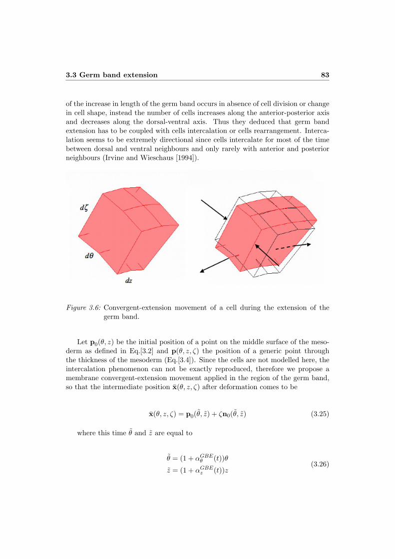
3.3 Germ band extension 83
of the increase in length of the germ band occurs in absence of cell division or changein cell shape, instead the number of cells increases along the anterior-posterior axisand decreases along the dorsal-ventral axis. Thus they deduced that germ bandextension has to be coupled with cells intercalation or cells rearrangement. Interca-lation seems to be extremely directional since cells intercalate for most of the timebetween dorsal and ventral neighbours and only rarely with anterior and posteriorneighbours (Irvine and Wieschaus [1994]).
Figure 3.6: Convergent-extension movement of a cell during the extension of thegerm band.
Let p0(+, z) be the initial position of a point on the middle surface of the meso-derm as defined in Eq.[3.2] and p(+, z, $) the position of a generic point throughthe thickness of the mesoderm (Eq.[3.4]). Since the cells are not modelled here, theintercalation phenomenon can not be exactly reproduced, therefore we propose amembrane convergent-extension movement applied in the region of the germ band,so that the intermediate position x(+, z, $) after deformation comes to be
x(+, z, $) = p0(+, z) + $n0(+, z) (3.25)
where this time + and z are equal to
+ = (1 + "GBE$ (t))+
z = (1 + "GBEz (t))z
(3.26)

84 Chapter 3. Morphogenetic movements in Drosophila embryo
with "GBE$ (t) and "GBE
z (t) the amplitudes respectively of the shortening fromthe dorsal to the ventral region of the embryo and of the lengthening along theanterior-posterior axis. They are expressed, as similarly as in Eq.[3.18], as
"GBE$ (t) = "$ · t
"GBEz (t) = "z · t
(3.27)
with "$ and "z specific constants. It has to be noticed here that for the for-mulation of the germ band extension we do not introduce the periodic functionneither for the deformation of + nor for the one of z. Actually, for the ventral andthe cephalic furrows, the modification of the active region is obtained through theprecise description of the change in shape of each single cell, therefore the need ofhaving for each element the same amplitude of deformation. In this specific case ofcells intercalation instead, the strain of the active region, which exactly correspondsto the germ band, is macroscopically obtained without reference to the individualcells.
Fia is here again computed from Eq.[3.6] and it is applied on the associated area
of deformation; its final expression is
FGBEa =
(1 + "GBE$ (t)),$
GBE
,$i$(+)" i$(+)
+(1 + "GBE
z (t)),GBEz
(1 + '$2(z)),z('$(z)ir(+) + iz))" ('$(z)ir(+) + iz)
+ n0(+, z)" n0(+, z)
(3.28)
with
,GBE$ = '(z) +
$/1 + '$2(z)
,GBEz = 1! $'$$(z)
(1 + '$2(z))3/2
(3.29)
3.4 Results
With the present work, we have been able to reproduce three morphogenetic move-ments: the ventral furrow invagination, the cephalic furrow formation and the germband extension. In this section we show the results for each individual simulation;the key aspects are presented together with the limits of the model and the improve-ments to be made, with particular emphasis on some parameters that may a!ect thefinal configurations and have to be taken into account. The results are interesting

3.4 Results 85
because in good agreement with the experimental observations, and innovative sincenever before, to our knowledge, a single FE model has allowed to reproduce morethan one morphogenetic movement (see Chapter 1). Furthermore, the analyticaldescription of the active forces on the cells consents to have di!erent expressions forthe active deformation gradients Fi
a that are therefore easy to modify and can becoupled together in order to have a concurrent simulation of two or three movementsat the time (see Chapter 4).
In this study, for sake of simplicity and because of the lack in information re-garding the mechanical characteristics of the vitelline membrane and the yolk, onlythe mesoderm is modelled. It is represented as an ellipsoid with the dimensions ofa real Drosophila embryo: 500µm in length, a cross-section diameter of 150µm anda thickness of 15µm (Fig. 3.7). When observing the real embryo, it is possible tonotice that the curvature is not the same all long the contour and there is not aperfect symmetry with respect to the vertical axis; actually the posterior pole ismore rounded than the anterior pole. Therefore the ellipsoid might not be the bestgeometrical representation; conscious of this drawback, we have also tested othersophisticated and accurate parametrical descriptions that allow us to take into ac-count such aspects (Sec. 3.11). As mentioned in Sec. 2.3, a Saint-Venant model isused to describe the mesoderm, thus only two parameters have to be chosen. TheYoung’s modulus E is set at 100Pa according to literature (Wiebe and Brodland[2005]). The Poisson’s coe"cient ) is fixed at 0.45 which gives a coe"cient of com-pressibility for the mesoderm km = E
3(1"2() = 333Pa. If the choice of the mechanicalcharacteristics of the mesoderm may appear here approximative, we want to remarkthat, for a biological system, and a fortiori for a micro-structure like the embryo, itis not always evident to detect all the parameters.
For the simulations, we have developed our own weak form and we have opted fora standard FE discretization, usually Lagrange elements of order two. The COM-SOL Multiphysics software (v 3.4; Comsol, Inc.) is used, a code that permits tomanipulate the governing equations. All the amplitudes "i(t) depend on an incre-mental parameter t, which varies between a minimal value timin, usually equal to 0,and a maximal value tiMAX , which changes according to the morphogenetic move-ment analyzed. Furthermore, the elementary forces are applied on the relative activedeformation region. Such region has almost the same dimensions of the active regionobserved in reality, where each event takes place, and is obtained by a regularizedHeaviside function. It consists of a C1 di!erentiable function whose value is 0 fora negative argument and 1 for a positive argument and it varies between these twovalues over a length fixed by us equal to one single cell ((= 15µm). This means that,for our specific case, we are going to have Fi
a as computed earlier for each movementwhere the deformation occurs, while elsewhere we will find Fi
a = I.Although the vitelline membrane and the yolk have not been physically rep-
resented and therefore not meshed here, both the boundary conditions have beenimplemented since the absence of one or both of them leads to final configurations
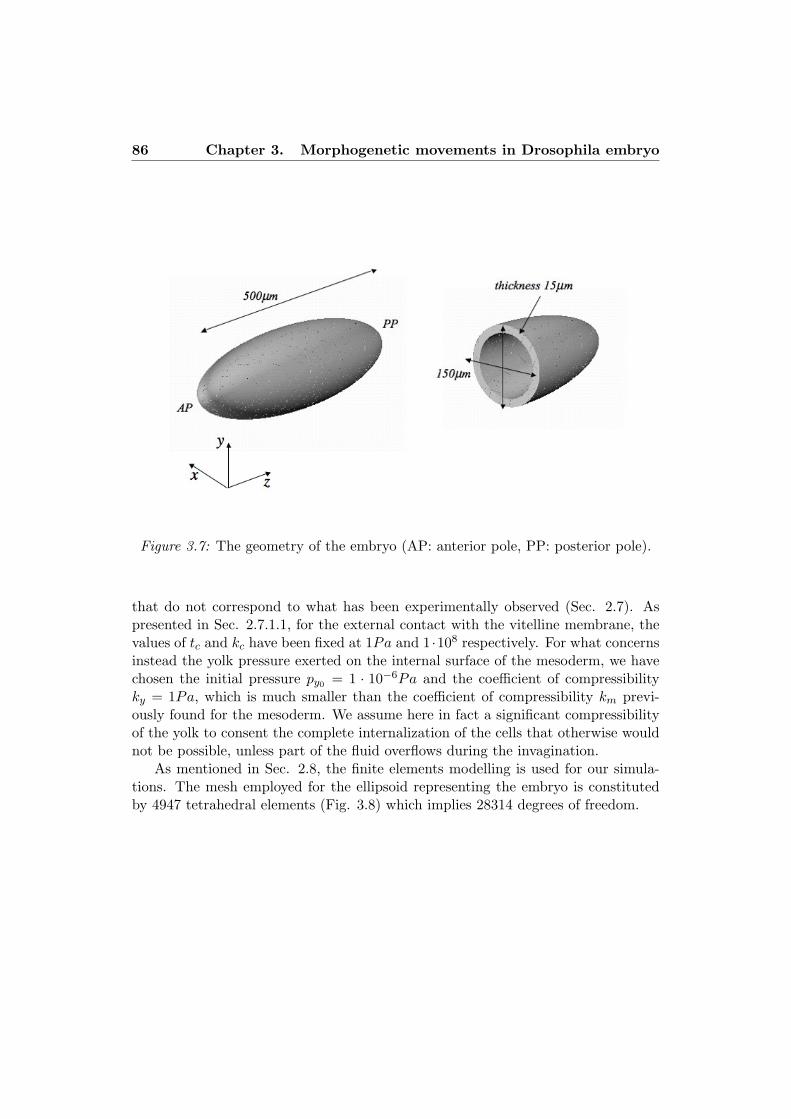
86 Chapter 3. Morphogenetic movements in Drosophila embryo
Figure 3.7: The geometry of the embryo (AP: anterior pole, PP: posterior pole).
that do not correspond to what has been experimentally observed (Sec. 2.7). Aspresented in Sec. 2.7.1.1, for the external contact with the vitelline membrane, thevalues of tc and kc have been fixed at 1Pa and 1 ·108 respectively. For what concernsinstead the yolk pressure exerted on the internal surface of the mesoderm, we havechosen the initial pressure py0 = 1 · 10"6Pa and the coe"cient of compressibilityky = 1Pa, which is much smaller than the coe"cient of compressibility km previ-ously found for the mesoderm. We assume here in fact a significant compressibilityof the yolk to consent the complete internalization of the cells that otherwise wouldnot be possible, unless part of the fluid overflows during the invagination.
As mentioned in Sec. 2.8, the finite elements modelling is used for our simula-tions. The mesh employed for the ellipsoid representing the embryo is constitutedby 4947 tetrahedral elements (Fig. 3.8) which implies 28314 degrees of freedom.

3.5 Ventral furrow invagination 87
Figure 3.8: The mesh employed for the geometry of the embryo. On the left aperspective view and on the right a cross sectional view.
3.5 Ventral furrow invagination
For the ventral furrow invagination we start by implementing only apical constrictionso that "abe(t) = 0 and Eq. [3.15] becomes
x(+, z, $) = p0(+, z) + $n0(+, z) (3.30)
The active deformation gradient FV FIa is then
FV FIa =
'1 + "ac(t)
2$
hm$(+)
(i$(+)" i$(+)
+
+'$(z)ir(+) + iz
,
(1 + '$2(z))"
)'$(z)ir(+) + iz
*
+'2"ac(t)
hm(+),$i$(+) + n0(+, z)
(" n0(+, z)
(3.31)
As we can deduce from Eq.[3.31], the final result for this simulation may bea!ected by several parameters such as the dimensions of the material cells and theamplitude of the active deformation region. In the next sections, we will focus on

88 Chapter 3. Morphogenetic movements in Drosophila embryo
the analysis of their influence on the final configuration, but for a first series of testswe have decided to fix them in order to have some preliminary results. Therefore inaddition to "abe(t) = 0, we set the amplitude of a single cell +cell = -/12.
The deformation region where the ventral furrow invagination takes place ischaracterized by:
• the length along the anterior-posterior axis, which remains constant and coversabout 70% (about 350µm) of the entire length of the embryo;
• the amplitude + along the cross section of the embryo, that is chosen for thisfirst specific case equal to 50!, which means about 60µm of the total circum-ference of the embryo (Fig. 3.9).
Figure 3.9: In red the active deformation region for the ventral furrow invagination(AP: anterior pole, PP: posterior pole). On the left a cross section ofthe embryo, on the right a ventral view.
If we assume that the dimensions of an embryonic cell are approximatively 15µmalong the apico-basal axis (equal to the thickness of the mesoderm since there is asingle layer of cells) and about 10µm along the anterior-posterior axis and the cross-section, we can deduce that the active region involves about 210 cells. Once theventral furrow has formed, we have almost 560 cells that have completely internalizedinto the yolk, which is not so di!erent from what it has been experimentally observed(Sec. 1.2.3). It has to be said that the qualitative dimensions chosen here for a singlecell have been deduced from images of real embryos and have to be considered thenas a reasonable average of multiple cases. One may notice a slight disagreement

3.5 Ventral furrow invagination 89
with respect to some parameters implemented for our simulations. For instance, thevalue of +cell provides a cross sectional length of a single cell approximatively equalto 15µm, which does not match with the dimension hypothezised above. This isdue to the fact that often the choice of the numerical variables have been made tosimultaneously assure the right properties of convergence and final consistent results.
For this specific simulation t goes from tV FImin = 0 to tV FI
MAX = 0.003. If weconsider the cell dimensions assumed above, the maximal value of "ac(t) = "ac ·tV FIMAX , where "ac is a constant, provides a maximal apical constriction for a single
cell of (= 7µm and therefore an almost equal basal elongation, according to theembryo curvature. Such maximal constriction corresponds to the maximal activedeformation, calculated by the analytical expression of the intermediate position xof any point of the mesoderm (Eq.[3.15]), and it would be observable if the cellswere totally free (see Sec. 2.1). Here instead, it does not coincide with the finaldeformation which is the composition of the active and the passive contributionsand thus larger or smaller according to the initial position of a cell.
In Fig. 3.10 we see the successive phases of ventral furrow invagination forour simulation. If we compare our results to the real invagination (Fig. 1.4), wenotice that in our case the mesoderm narrows much more than in reality, whichleads to a greater self-contact between the two strips of the mesoderm. So far wedid not analyzed this phenomenon from a theoretical point of view, even if thistype of contact could engender repulsive forces and a!ects the global behaviourof the system. Nevertheless, the vertical symmetry of the embryo is not brokenso that the self-contact is naturally taken into account. Additionally, throughoutthe simulations, we have observed how some parameters may favor or inhibit suchphenomenon.
The last image (Fig. 3.10d, cross section) represents the material cells that areobtained here by a cell marker (Heaviside function) transported by the deformationmovement. Each white sector defines a single cell that undergoes the elementarydeformations, while the black zones correspond to the transition between the twovalues of the smooth step function; the more the mesoderm invaginates, the morethe apical constriction is evident, particularly at the peak of the furrow, where theapical surfaces are almost completely shrink. Additionally the constriction switchesfrom apical to basal according to the mesoderm wedging; specifically, as alreadymentioned in Sec. 3.2, they are apically constricted at the medio-lateral hinge point,while basally at the dorso-lateral hinge points. It has to be noticed that, if at themedio-lateral hinge point, which is included in the active region, the deformation istriggered by Fa, at the dorso-lateral hinge points the basal constriction is due to thepassive reaction of the tissues Fm.
These preliminary results confirm what has been pointed out by biologists (seeSec. 1.2.3). In fact we find that, introducing only the apical constriction as activeelementary deformation on the cells, the ventral furrow invagination still takes place.This means that apical constriction is e!ectively an active force acting on the cells,
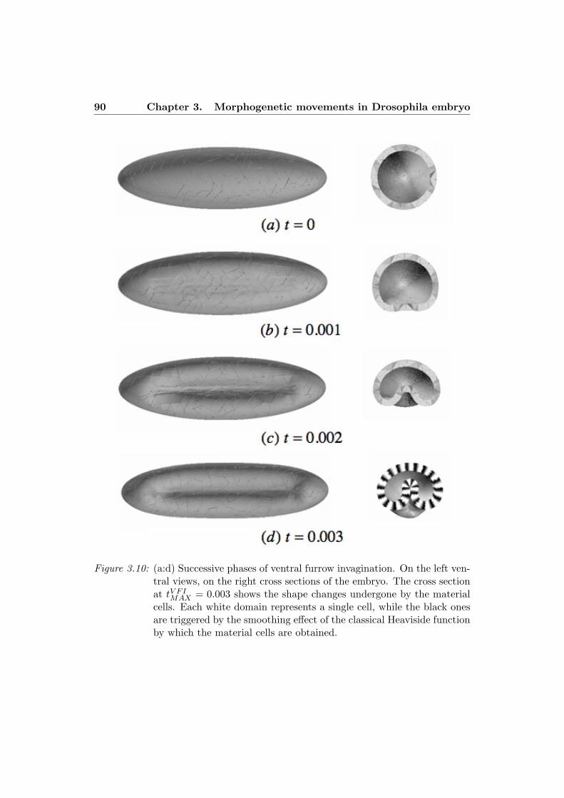
90 Chapter 3. Morphogenetic movements in Drosophila embryo
Figure 3.10: (a:d) Successive phases of ventral furrow invagination. On the left ven-tral views, on the right cross sections of the embryo. The cross sectionat tV FI
MAX = 0.003 shows the shape changes undergone by the materialcells. Each white domain represents a single cell, while the black onesare triggered by the smoothing e!ect of the classical Heaviside functionby which the material cells are obtained.
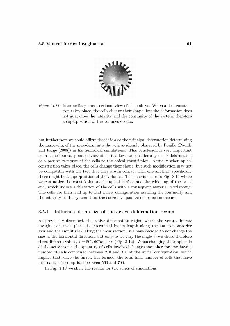
3.5 Ventral furrow invagination 91
Figure 3.11: Intermediary cross sectional view of the embryo. When apical constric-tion takes place, the cells change their shape, but the deformation doesnot guarantee the integrity and the continuity of the system; thereforea superposition of the volumes occurs.
but furthermore we could a"rm that it is also the principal deformation determiningthe narrowing of the mesoderm into the yolk as already observed by Pouille (Pouilleand Farge [2008]) in his numerical simulations. This conclusion is very importantfrom a mechanical point of view since it allows to consider any other deformationas a passive response of the cells to the apical constriction. Actually when apicalconstriction takes place, the cells change their shape, but such modification may notbe compatible with the fact that they are in contact with one another; specificallythere might be a superposition of the volumes. This is evident from Fig. 3.11 wherewe can notice the constriction at the apical surface and the widening of the basalend, which induce a dilatation of the cells with a consequent material overlapping.The cells are then lead up to find a new configuration assuring the continuity andthe integrity of the system, thus the successive passive deformation occurs.
3.5.1 Influence of the size of the active deformation region
As previously described, the active deformation region where the ventral furrowinvagination takes place, is determined by its length along the anterior-posterioraxis and the amplitude + along the cross section. We have decided to not change thesize in the horizontal direction, but only to let vary the angle +; we chose thereforethree di!erent values, + = 50!, 60!and 90! (Fig. 3.12). When changing the amplitudeof the active zone, the quantity of cells involved changes too; therefore we have anumber of cells comprised between 210 and 350 at the initial configuration, whichimplies that, once the furrow has formed, the total final number of cells that haveinternalized is comprised between 560 and 700.
In Fig. 3.13 we show the results for two series of simulations

92 Chapter 3. Morphogenetic movements in Drosophila embryo
Figure 3.12: Variation of the active deformation region for VFI. (a) + = 50! (b)+ = 60! (c) + = 90!.
• images (a:c) represent the invagination with +cell = -/10 and + = 50!(a),60!(b) and 90!(c)
• for images (d:f), +cell is set to -/12 and again + varies from 50!(a), 60!(e) and90!(f)
When modifying the dimensions of the active region of deformation, we expectedthat the greater +, the higher the invagination of the mesoderm into the yolk, butactually this is really evident only for the case of + = 90! (Fig. 3.13c) and evenmore for the case with +cell = -/12 (Fig. 3.13f). On the other hand, we observethat the self-contact decreases when the active region increases, leading to a widerinvagination.
3.5.2 Influence of the dimensions of the material cells
The next parameter we are going to analyze is +cell, which determines the dimensionsof a single cell by which the mesoderm is divided along the cross section. It has tobe said that, for the simulation of the ventral furrow invagination, we have supposedthat the cells do not deform along the anterior-posterior axis, which means thattheir size in the z direction remains constant. Therefore we have only changed thedimensions along +; specifically, we have tested +cell = -/8, -/10 and-/12. Thelesser the value of +cell, the higher the number of the cells in the domain. Suchvalues for +cell may not be very accurate since, observing a real embryo, we cancount up to 80 cells along the cross-section at z = 0. According to the hypothesismade in Sec. 3.5 concerning the dimensions of a single cell and given the dimensionsof the embryo, we find about 42 cells along the section. This theoretical numberof cells is still too big compared to the maximal one obtained for our simulations

3.5 Ventral furrow invagination 93
Figure 3.13: Influence of the size of the active deformation region on the ventralfurrow invagination; cross sections of the embryo at tV FI
MAX = 0.003.(a:c) Simulations with +cell = -/10 and the amplitude + of the regionequal to 50!(a), 60!(b) and 90!(c). (d:f) Simulations with +cell = -/12and again + = 50!(d), 60!(e) and 90!(f).
when +cell = -/12, which provides 24 cells. If we consider that +cell corresponds to agroup of 3 cells on which the active forces are applied, we obtain a total number ofcells along the section equal to 72 which is therefore reasonable compared to reality.This hypothesis allows to optimize the quality of the convergence properties assuringcoherent final results.
Fig. 3.14 shows the results obtained for this specific analysis, for which the sizeof the active deformation region is the same as for the first study, with + = 50!
(Sec. 3.5). We remark that the more the material cells composing the mesoderm,the more evident and accentuated the self-contact between the mesodermal stripsand additionally there is a better continuity at the medio-lateral hinge point.
3.5.3 Influence of the apico-basal elongation
The previous tests not only provide a parametric study for the simulation of theventral furrow invagination, but they also allow us to define the best set of param-eters giving the most consistent and similar final configuration compared to reality.Therefore for the next simulations we have fixed the dimensions of the material cells+cell = -/12 and the amplitude of the active region + = 50!.
When introducing the apico-basal elongation, the intermediate position x is again

94 Chapter 3. Morphogenetic movements in Drosophila embryo
Figure 3.14: Influence of the dimensions of the cells. Cross sections of the em-bryo at tV FI
MAX = 0.003; the white spots represent a single cell, whilethe black ones are triggered by the smoothing e!ect of the classi-cal Heaviside function by which the cells are obtained. The size ofthe deformation region is still the same (+ = 50!), while +cell =-/8 (a), -/10 (b) and-/12 (c).
Figure 3.15: Influence of the apico-basal elongation on the ventral furrow invagina-tion; cross sections of the embryo at tV FI
MAX = 0.003. (a) Simulationwith only apical constriction implemented (b) Simulation with boththe elementary cell deformations taken into account.
the one expressed in Eq.[3.15], so that the parameter "abe(t) defines the elongationof the cells along their apico-basal axis. Considering the tV FI
min and tV FIMAX previously
indicated (Sec. 3.5), the maximal value for "abe(t) = "abe · tV FIMAX , where "abe is a
constant, provides a maximal apico-basal elongation equal to (= 2 · 10"2µm. As wesee in Fig. 3.15b, the presence of this additional elementary deformation does notplay a significant role for what concerns the size of the invagination, which is almostthe same compared to the simulation where only apical constriction is considered;nevertheless it highly inhibits the self-contact.
3.6 Cephalic furrow formation 95
3.6 Cephalic furrow formation
The formation of the cephalic furrow is induced by a narrowing of the mesodermalong the horizontal axis over the entire cross section of the embryo; this means thatthe apical constriction, which, given the considerations made in Sec. 3.5, is againthe only elementary force introduced, involves a deformation along the z direction(Eq.[3.19]). Compared to the ventral furrow, the simulation of the cephalic furrowwould have been more complex if some simplifications would have not been done.Actually the ventral furrow, throughout its formation, maintains a position parallelto the anterior-posterior axis. On the other hand the cephalic furrow starts to formvertically but then, probably triggered by the extension of the germ band, whichstarts to take place at that moment of gastrulation, it is pushed forward towards theanterior pole and its final position results to be inclined at about 30! with respectto the dorsal-ventral axis of the embryo. Therefore the cells constrict apically inthe z direction and additionally they skew, so that their + (Eq.[3.19]) changes asthe process goes along. Technically this issue could have been handled either byimplementing a deformed + in the equation of the intermediate position x or byusing a Eulerian formulation instead of a Lagrangian one. For the present work wehave decided to leave aside the analysis of this peculiar aspect, which is however inprogress and probably presented for further studies. To sum up, we have modelledthe active deformation region for the cephalic furrow as showed in Fig. 3.16: parallelto the vertical axis of the embryo, at about one third of the total horizontal length,and fixed throughout the simulation.
The simulation starts at tCFmin = 0 and stops at tCF
MAX = 0.001; the maximalapical constriction for a single cell in the z direction is obtained when "ceph(t) ="ceph · tCF
MAX , "ceph being a constant, and is equal to (= 5µm. Here again it has tobe noticed that the maximal active constriction has been obtained from the inter-mediate position x (Eq.[3.19]) and therefore does not represent the final observeddeformation, which is however the result of the active and the passive contributions.The results are presented in Fig. 3.17. The maximal active deformation leadingto the formation of the cephalic furrow is much smaller than the one found for theventral furrow invagination; this is probably due to the fact that the active regionfor this specific simulation is thinner, thus a slighter number of cells is involved andalso that the amplitude of the invagination is smaller in this case.
Finally we want to point out once more that here again only apical constriction isintroduced as elementary deformation of the cells and we still obtain the invaginationof the mesoderm giving the formation of the cephalic furrow; our previous conclusionis then reconfirmed.

96 Chapter 3. Morphogenetic movements in Drosophila embryo
Figure 3.16: Perspective (top) and cross sectional (bottom) views of the embryo.In red the active deformation region for cephalic furrow (AP: anteriorpole, PP: posterior pole).
Figure 3.17: (a) Cross sectional view of the embryo at the final configuration(tCF
MAX = 0.001) for the simulation of the cephalic furrow (b) Globalview of the embryo.

3.7 Germ band extension 97
3.7 Germ band extension
The germ band extension has been the first morphogenetic event we have tried toreproduce since the main objective was to compare the numerical results with theexperimental ones obtained by Farge and co-workers (Supatto et al. [2005]). Theydetected the velocity field of an intact embryo during the convergent-extension move-ment of the cells and they also observed that the extension of the germ band leadsto a compression at the anterior pole of the embryo. Such compression induces theexpression of the gene twist, which normally is only expressed at the ventral region(Brouzes and Farge [2004], Farge [2003]). Biologists have therefore supposed that, ifthe genes control the mechanical movements of the embryo (see Chapter 1), also theother way round may be possible, which means that morphogenetic events influenceand regulate the expression of certain genes within the embryo. This phenomenon isknown as mechanotransduction and refers thus to the many mechanisms by whichcells convert a mechanical stimulus into chemical activity. We have been able to es-timate the induced forces through the embryo when the convergent-extension move-ment takes place (Sec. 3.9, 3.10); the results are coherent with what has been foundby biologists and therefore constitute an important support for further analysis.
In Fig. 3.18 the active deformation region defined for the present simulation isrepresented in red; it covers approximatively 40% of the entire length of the embryoalong the anterior-dorsal axis ((= 200µm) and it has an amplitude of about 90!
((= 100µm). Therefore, according to the hypothesis made for the dimensions ofa single cell (Sec. 3.5), about 200 cells are involved in the convergent-extensionmovement.
In Eq.[3.25], which supplies the intermediate position x during germ band ex-tension, we indicate with "GBE
$ (t) and "GBEz (t) the amplitudes of the convergence
and the extension of the cells respectively; their values have been chosen assuminga regular intercalation of the cells. This means that, given the fact that the cellsdo not divide nor bind together, the initial number of cells involved is the same atthe end of the simulation. Therefore, if at the initial configuration (tGBE
min = 0) wehave approximatively 20 cells along the anterior-posterior axis and 10 cells along thedorsal-ventral axis in the active region, at the final configuration (tGBE
MAX = 0.02),since the germ band has undergone an elongation of about 50µm and a shorten-ing of 20µm, we find 25 and 8 cells respectively along the anterior-posterior anddorsal-ventral axes. The amplitude of the elongation does not correspond here tothe experimental data (Sec. 1.2.7), according to which the germ band almost dou-bles its length; this is due to the fact that our simulation reproduces only part of theconvergent-extension process, so that the mass movement is not fully completed.
The results are shown in Fig. 3.19. It is possible to outline a confined area ofthe dorso-lateral region of the embryo where the cells converge and shorten; on theside boundary of the area instead, the cells start to elongate and they are involvedin whirlpool movements, in particular at the posterior pole.

98 Chapter 3. Morphogenetic movements in Drosophila embryo
Figure 3.18: In red the active deformation region for the germ band extension; crosssection (left) and ventral (right) views (AP: anterior pole, PP: posteriorpole).
Figure 3.19: Frontal view of the embryo for the simulation of the germ band exten-sion (tGBE
MAX = 0.02). The black arrows represent the displacements.
The constitutive law adopted for the present work does not depend on time,but we have tried, through a calibration, to estimate the velocity by which thetissues deform and we have compared it with experimental data. The germ bandextension of a real Drosophila embryo takes approximatively 2h to complete, with afinal elongation of about 2.5 times the initial length. In our simulation, at the initialconfiguration, the active region covers 200µm, which means that theoretically it
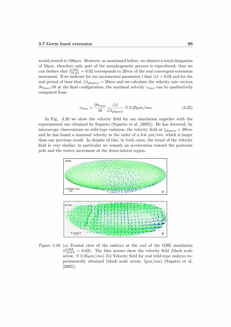
3.7 Germ band extension 99
would stretch to 500µm. However, as mentioned before, we observe a total elongationof 50µm, therefore only part of the morphogenetic process is reproduced; thus wecan deduce that tGBE
MAX = 0.02 corresponds to 20mn of the real convergent-extensionmovement. If we indicate for our incremental parameter t that&t = 0.02 and for thereal period of time that &tphysics = 20mn and we calculate the velocity rate vectors%umax/%t at the final configuration, the maximal velocity vmax can be qualitativelycomputed from
vmax =%umax
%t
&t
&tphysics
(= 0.25µm/mn (3.32)
In Fig. 3.20 we show the velocity field for our simulation together with theexperimental one obtained by Supatto (Supatto et al. [2005]). He has detected, bymicroscopy observations on wild-type embryos, the velocity field at tphysics = 29mnand he has found a maximal velocity in the order of a few µm/mn, which is largerthan our previous result. In despite of this, in both cases, the trend of the velocityfield is very similar; in particular we remark an acceleration toward the posteriorpole and the vortex movement at the dorso-lateral region.
Figure 3.20: (a) Frontal view of the embryo at the end of the GBE simulation(tGBE
MAX = 0.02). The blue arrows show the velocity field (black scalearrow, (= 0.25µm/mn) (b) Velocity field for real wild-type embryo ex-perimentally obtained (black scale arrow, 5µm/mn) (Supatto et al.[2005]).

100 Chapter 3. Morphogenetic movements in Drosophila embryo
3.8 Hyperelastic model tested for GBE
As described in Sec. 2.3, we have chosen to model the mesoderm as a Saint-Venantmaterial, which is probably not the best approach for our problem for two principalreasons. First of all, in previous works we often found a hyperelastic analysis of themechanical characteristics of the embryo. Secondly, we are aware that the embryonictissues show visco-elastic properties that are therefore not taken into account here,but may strongly a!ect the global behaviour of the system.
In order to catch up with these drawbacks, we have decided first to make a com-parison between our model, which is simple and linear, and the hyperelastic modelsproposed in literature. In Sec. 2.3 we have pointed out the fact that the equationdescribing the Neo-Hookean material, which is a particular case of a Mooney-Rivlinmaterial, corresponds to a quadratic form of the Saint-Venant model (Eq.[2.47]).By a power extension linearized to the first order of the Neo-Hookean constitutivelaw and imposing a vanishing initial stress, we are able, from Eq.[2.48], to deducethe values for "1 and "2, which are defined for the hyperlastic model considered.Therefore we obtain for our specific case that "1 = µL/2 * 17 and "2 = µL/2 * !17(µL is the classical Lame’s coe"cient defined in Eq.[2.37]).
Figure 3.21: Simulation of the GBE with a hyperelastic model; the arrows representthe displacements field. The results show a high similarity with theones with a Saint-Venant model.
We have tested the hyperelastic model for the GBE simulation. The new param-eters previously found have been implemented and we have replaced the expressionof the Second Piola-Kirchho! tensor (Eq.[2.44]) with the new one in the PVP for-mulation. The results are very similar to the ones obtained in Sec. 3.7. It is possibleto see a beginning of the vortex movement at the posterior pole of the embryo eventough the convergence from the dorsal to the ventral region is less worsen. At the

3.9 Estimation of the induced forces through the embryo 101
maximal values "GBE$ (t) = "$ · tGBE
MAX and "GBEz (t) = "z · tGBE
MAX , t varying between0 and 0.023, we find a maximal elongation and shortening of the germ band respec-tively of about 56µm and 23µm. Such values are not so di!erent from the onesfound with a Saint-Venant model (Sec. 3.7); we can then conclude that our firstchoice can be considered appropriate for the analysis of our problem.
3.9 Estimation of the induced forces through the em-bryo
In the present study, the gradient decomposition method allows us to take intoaccount the active and the passive forces that provide the final configuration foreach morphogenetic movement that we simulate. The passive forces are consideredas a consequent response to the active ones that have been individuated by biologiststhrough experimental observations. It is still di"cult to detect which ones among theelementary deformations acting on the cells have to be hold as active and which onesas passive forces. In particular this is evident for the ventral furrow invagination(Sec. 1.2.3) where five movements have been observed and only two of them areconsidered as active. Contrarily our simulations have pointed out that even whenonly one of these elementary forces, specifically apical constriction, is implementedwe still obtain the invagination of the mesoderm into the yolk (Sec. 3.5).
So far the active forces are directly introduced into our formulation but they areactually engendered by chemical signals developing within the embryo that are nottaken into account here. Similarly, we are aware that the passive forces produced atthe active regions and responsible, in our specific case, for the formation of the ven-tral and the cephalic furrows and the germ band extension, may in turn trigger newactive forces elsewhere in the embryo. This key aspect has been amply studied byFarge and co-workers for the germ band extension. In fact they have demonstratedthat the tissues extension at the ventral region leads to a consequent pressure at theanterior pole where, therefore, the expression of the twist, a gene which normally isonly ventrally expressed, is observed (Brouzes and Farge [2004], Farge [2003]). Thismeans that not only there is a continuous and concatenate series of mechanical forcesdeveloping during embryogenesis, but also and more importantly that such forcesmay highly influence the expression of specific genes also at long distance in theembryo, which implies a mechanotransduction pattern throughout the development.
For this reason we believe it is important to evaluate how the tissues adjacent tothe active regions respond and behave when the active forces are applied. In orderto do so, we are going to analyze the volume variation &V within the mesoderm,which indicates if the cells compress or expand. We can write
&V =dV ! dV0
dV0=
dV
dV0! 1 = detF! 1 (3.33)
102 Chapter 3. Morphogenetic movements in Drosophila embryo
From the definition of the Right Cauchy-Green deformation tensor C (Eq.[A.11]),we have
C = FTF = I + 2E (3.34)
(detF)2 = det(I + 2E) (3.35)
Then, by a 1st order approximation, we obtain
detF (= 1 + trE (3.36)
and Eq.[3.33] becomes
&V (= trE (3.37)
Consequently, the pressure force that can be engendered within the embryo iscalculated as
pm =trSm
3= kmtrEm =
E
3(1! 2 ))trEm (3.38)
where Sm is the Second Piola-Kirchho! tensor which provides the constitutivelaw of the mesoderm (Eq.[2.35]), km is the coe"cient of compressibility for themesoderm and Em is the Green-Lagrange tensor as defined in Eq.[2.36], which variesbetween the active and the passive regions.
We are now going to estimate, for each morphogenetic movement, the magnitudeof the induced pressure forces. First of all it has to be noticed that for the simulationof the ventral and the cephalic furrows the strains are highly concentrated at theactive zone, so that the forces slightly spread around. In the case of the germ bandextension instead, we observe that, even if at a lower rate, the strains can also betransmitted at long distance, as later on described.
For the ventral furrow (when both apical constriction and apico-basal elongationare implemented) we observe the elongation of the basal surfaces of the cells at themedian hinge point, while the apical surface are constricted as expected; also tissuesextend internally at the dorso-lateral hinge points, even if the amplitude of suchextension is much smaller than the former one (Fig. 3.22). The same observationscan be drawn for the cephalic furrow where, according to the elementary active forceintroduced (apical constriction), we have a compression of the cells on the externalsurface, while they enlarge at the internal surface. From a quantitative point ofview it is possible to estimate the range of values for pV FI
m and pCFm in the active
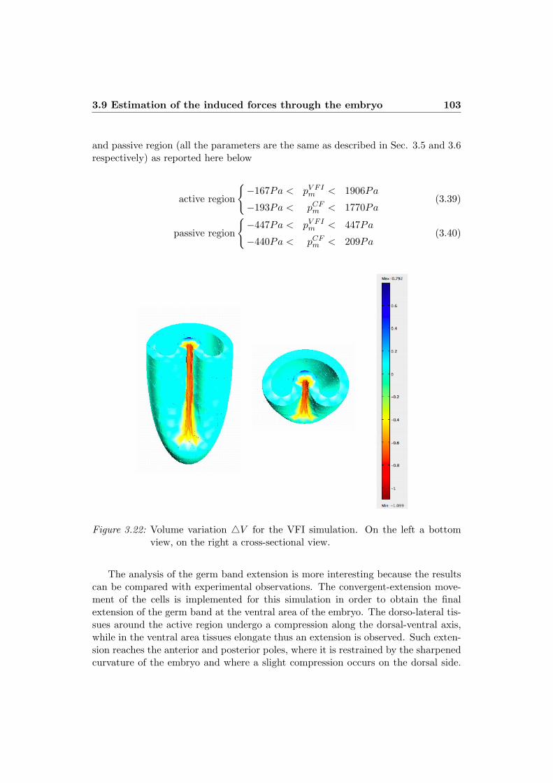
3.9 Estimation of the induced forces through the embryo 103
and passive region (all the parameters are the same as described in Sec. 3.5 and 3.6respectively) as reported here below
active region
0!167Pa < pV FI
m < 1906Pa
!193Pa < pCFm < 1770Pa
(3.39)
passive region
0!447Pa < pV FI
m < 447Pa
!440Pa < pCFm < 209Pa
(3.40)
Figure 3.22: Volume variation &V for the VFI simulation. On the left a bottomview, on the right a cross-sectional view.
The analysis of the germ band extension is more interesting because the resultscan be compared with experimental observations. The convergent-extension move-ment of the cells is implemented for this simulation in order to obtain the finalextension of the germ band at the ventral area of the embryo. The dorso-lateral tis-sues around the active region undergo a compression along the dorsal-ventral axis,while in the ventral area tissues elongate thus an extension is observed. Such exten-sion reaches the anterior and posterior poles, where it is restrained by the sharpenedcurvature of the embryo and where a slight compression occurs on the dorsal side.

104 Chapter 3. Morphogenetic movements in Drosophila embryo
It is possible to locally evaluate the volume variation so that we find &V = !0.0014and &V = !0.007 respectively at the anterior and the posterior pole (Fig. 3.23).The negative sign clearly indicates a compression of the cells whose magnitude isin the order of the mean sagittal deformation that have been experimentally de-termined (Desprat et al. [2008], Supatto [2005]). The estimated pressure when thegerm band extension occurs can be calculated again for the active and the passiveregions and we obtain
0active region !13Pa < pGBE
m < 23Pa
passive region !43Pa < pGBEm < 7Pa
(3.41)
and specifically at the anterior and the posterior pole, which are included inthe passive region, we find !0.46Pa and !2.33Pa respectively. These data confirmtherefore, from a qualitative point of view, the experimental observations that showthe presence of a compression at the anterior pole. In order to have a quantitativeanalysis, it would be necessary to evaluate the magnitude of the real pressure, tocompare it with the value found for our simulation.
Figure 3.23: Volume variation &V for the GBE simulation. Here the values scalehas been adapted to highlight the e!ects on the anterior and posteriorpole.
3.10 Estimation of the induced shear stress through the embryo 105
3.10 Estimation of the induced shear stress through theembryo
If the variation of the mesoderm volume previously calculated indicates how thecells compress or expand, the norm of the deviator of the Green-Lagrange tensorEm for the passive deformation, as similarly as for the Von Mises criterion, consentsto determine how the cells behave with respect to one another. It provides the dis-tribution of the shear deformations through the mesoderm domain and it is definedas follows
+dev Em+ =8
E2mxx
+ E2myy
+ E2mzz
!EmxxEmyy !EmyyEmzz !EmxxEmzz
+3E2mxy
+ 3E2myz
+ 3E2mxz
(3.42)
For the germ band extension, when the parameters are the same as the onesobtained in Sec. 3.7, we find dev Em = 0.01 and dev Em = 0.014 respectively atthe anterior and the posterior pole. In order to estimate the magnitude of thestrain induced at the two poles by the extension of the germ band, dev Em can becompared, at first approximation, to the shear deformation ., so that we can write
! = µ . * µL+devEm+ (3.43)
where ! is the shear stress and µL the Lame’s coe"cient (Eq.[2.37]). Therefore,having µL = 34.4, we obtain !GBE * 0.34Pa at the anterior pole and !GBE * 0.48Paat the posterior pole; globally !GBE varies from a minimal value of about 0.01Pa toa maximal value of 6.88Pa. For the ventral and the cephalic furrow we find instead0.13Pa < !V FI < 198Pa and 0.07Pa < !CF < 190Pa respectively; these valuesare largely greater than the ones obtained for the GBE, where the strains are lessconcentrated and may be transmitted at long distance within the embryo. Actually,if we ma ke a comparison with experimental data, we notice that the maximal valuefor !GBE is in the order of the laminar shear stress applied on cells placed in abioreactor over 24h, that is usually comprised between 10 and 30Pa (Traub andBerk [1998]). At this intensity the shear stress may induce several cellular e!ectssuch as coagulation, migration, proliferation or adhesion.
3.11 Influence of the geometry on VFI and GBE
As described in Sec. 3.1, the embryo is parametrically represented here by an el-lipsoid in a cylindrical coordinates system. However, the real embryo presents anon-perfect symmetry between the anterior and the posterior pole which may in-fluence those morphogenetic movements that take place along the horizontal axis.
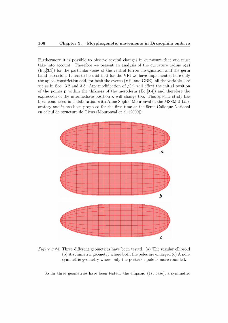
106 Chapter 3. Morphogenetic movements in Drosophila embryo
Furthermore it is possible to observe several changes in curvature that one musttake into account. Therefore we present an analysis of the curvature radius '(z)(Eq.[3.3]) for the particular cases of the ventral furrow invagination and the germband extension. It has to be said that for the VFI we have implemented here onlythe apical constriction and, for both the events (VFI and GBE), all the variables areset as in Sec. 3.2 and 3.3. Any modification of '(z) will a!ect the initial positionof the points p within the thikness of the mesoderm (Eq.[3.4]) and therefore theexpression of the intermediate position x will change too. This specific study hasbeen conducted in collaboration with Anne-Sophie Mouronval of the MSSMat Lab-oratory and it has been proposed for the first time at the 9eme Colloque Nationalen calcul de structure de Giens (Mouronval et al. [2009]).
Figure 3.24: Three di!erent geometries have been tested. (a) The regular ellipsoid(b) A symmetric geometry where both the poles are enlarged (c) A non-symmetric geometry where only the posterior pole is more rounded.
So far three geometries have been tested: the ellipsoid (1st case), a symmetric

3.11 Influence of the geometry on VFI and GBE 107
geometry with respect to the vertical axis where the poles are enlarged (2nd case),an asymmetric case with only one enlarged pole (3rd case) (Fig. 3.24). All thegeometries are obtained using the loft function in Matlab, which allows to constructa three dimensional object from an adjacent series of two dimensional surfaces.
1st case
The first case is represented by the ellipsoid that is parametrically obtained by'(z) as defined in Eq.[3.3] (Fig. 3.24a).
2nd case
Here the symmetry with respect to the vertical axis is maintained, but the radius'(z) is modified and can be written as
'(z) = b
31!
-z
a
.4(3.44)
which provides a global geometry as in Fig. 3.24b, where the two poles are morerounded than for the ellipsoid.
3rd case
The third case is a combination of the classical ellipsoid (1st case) and the pre-vious geometry (2nd case). Actually '(z) changes according to the horizontal coor-dinate as follows
9::;
::<
z < 0 '(z) = b
31!
-z
a
.2
z > 0 '(z) = b
31!
-z
a
.4(3.45)
so that the embryo is represented as in Fig. 3.24c. This geometry better repro-duces the real embryo since the symmetry with respect to the dorsal-ventral axis ofthe embryo is no more respected and only the posterior pole is more rounded.
Results
When comparing the three cases for the VFI (Fig. 3.25, 3.26), we observe agreater invagination for the case of the ellipsoid for any z considered and in particularat z = 0. The invagination for the the 3rd case is asymmetric and similar to thefirst case for z < 0 and to the second one for z > 0, while at z = 0 the amplitude isintermediary between the two previous cases.

108 Chapter 3. Morphogenetic movements in Drosophila embryo
Figure 3.25: Frontal sections of the ventral furrow invagination for the 1st geometry(a), the 2nd (b) and the 3rd (c).
Figure 3.26: Cross sections of the ventral furrow invagination. (a) and (b) representthe 1st and the 2nd geometries, while (c) and (d) correspond to z < 0and z > 0 respectively for the 3rd case.

3.11 Influence of the geometry on VFI and GBE 109
For the simulation of the GBE (Fig. 3.27) it is evident from the 2nd and the3rd geometries that when the anterior or the posterior pole are more rounded, thetissues are able to extend more toward the dorsal region of the embryo than for thecase of the regular ellipsoid. Such greater elongation at the posterior pole is actuallyobserved in real embryos and, because of the presence of the cephalic furrow whichconstipate the displacements, leads to the formation of little invaginations at thedorsal region that are not reproduced for our simulation.
Figure 3.27: Results for the GBE when the three geometries are used (a) 1st case(b) 2nd case (c) 3rd case.
These results show how a local change of '(z) may non-locally influence thefinal configurations because of the longitudinal displacements. In particular a largercurvature of the poles influences the global displacements, especially for the case ofthe GBE at the posterior pole. On the other hand the non-symmetry with respectthe dorsal-ventral axis of the embryo does not provide evident di!erences betweenthe anterior and the posterior poles for what concerns the deformations. At presentwe are working on two other geometries that take into account the flattening of
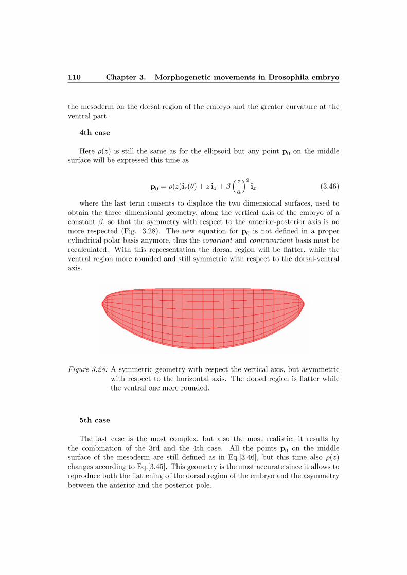
110 Chapter 3. Morphogenetic movements in Drosophila embryo
the mesoderm on the dorsal region of the embryo and the greater curvature at theventral part.
4th case
Here '(z) is still the same as for the ellipsoid but any point p0 on the middlesurface will be expressed this time as
p0 = '(z)ir(+) + z iz + *-z
a
.2ix (3.46)
where the last term consents to displace the two dimensional surfaces, used toobtain the three dimensional geometry, along the vertical axis of the embryo of aconstant *, so that the symmetry with respect to the anterior-posterior axis is nomore respected (Fig. 3.28). The new equation for p0 is not defined in a propercylindrical polar basis anymore, thus the covariant and contravariant basis must berecalculated. With this representation the dorsal region will be flatter, while theventral region more rounded and still symmetric with respect to the dorsal-ventralaxis.
Figure 3.28: A symmetric geometry with respect the vertical axis, but asymmetricwith respect to the horizontal axis. The dorsal region is flatter whilethe ventral one more rounded.
5th case
The last case is the most complex, but also the most realistic; it results bythe combination of the 3rd and the 4th case. All the points p0 on the middlesurface of the mesoderm are still defined as in Eq.[3.46], but this time also '(z)changes according to Eq.[3.45]. This geometry is the most accurate since it allows toreproduce both the flattening of the dorsal region of the embryo and the asymmetrybetween the anterior and the posterior pole.
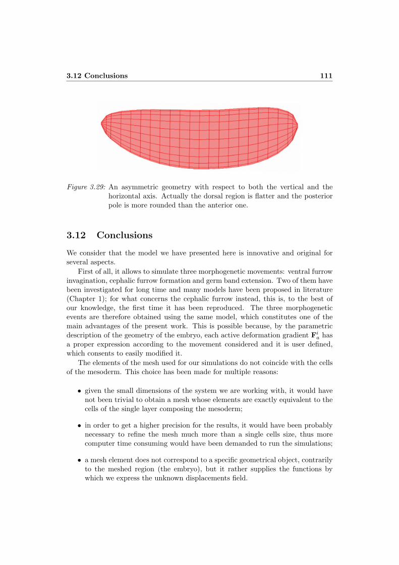
3.12 Conclusions 111
Figure 3.29: An asymmetric geometry with respect to both the vertical and thehorizontal axis. Actually the dorsal region is flatter and the posteriorpole is more rounded than the anterior one.
3.12 Conclusions
We consider that the model we have presented here is innovative and original forseveral aspects.
First of all, it allows to simulate three morphogenetic movements: ventral furrowinvagination, cephalic furrow formation and germ band extension. Two of them havebeen investigated for long time and many models have been proposed in literature(Chapter 1); for what concerns the cephalic furrow instead, this is, to the best ofour knowledge, the first time it has been reproduced. The three morphogeneticevents are therefore obtained using the same model, which constitutes one of themain advantages of the present work. This is possible because, by the parametricdescription of the geometry of the embryo, each active deformation gradient Fi
a hasa proper expression according to the movement considered and it is user defined,which consents to easily modified it.
The elements of the mesh used for our simulations do not coincide with the cellsof the mesoderm. This choice has been made for multiple reasons:
• given the small dimensions of the system we are working with, it would havenot been trivial to obtain a mesh whose elements are exactly equivalent to thecells of the single layer composing the mesoderm;
• in order to get a higher precision for the results, it would have been probablynecessary to refine the mesh much more than a single cells size, thus morecomputer time consuming would have been demanded to run the simulations;
• a mesh element does not correspond to a specific geometrical object, contrarilyto the meshed region (the embryo), but it rather supplies the functions bywhich we express the unknown displacements field.
112 Chapter 3. Morphogenetic movements in Drosophila embryo
The elementary active forces introduced for each movement are then mesh inde-pendent, but it is however possible to visualize, through specific analytical markers,the material cells and the relative deformations that they undergo all long the sim-ulation.
To represent the mesoderm we have decided to use a Saint-Venant material,which may appear at first sight an approach too simplistic and approximative for ourproblem, since we are treating with a biological system where many parameters haveto be taken into account. Although, we have extensively compared the constitutivelaw we use with the models found in literature and have also showed that the resultsobtained for our simulations, specifically for the germ band extension, are not sodi!erent from the ones obtained for a Neo-Hookean material (Sec. 3.8). Thereforeour choice results appropriate and the linearity of the constitutive law consents toskip out material’s constants that are usually very di"cult to detect. Nevertheless,so far we have not taken into account the visco-elasticity of the mesoderm, whichmay play a significant role and may a!ect the global response of the embryo. Thisis one of the aspects we would like to develop in the future and on which we areworking in order to have a model completely coherent with the reality.
The simulation of the ventral furrow invagination provides very interesting re-sults; if we compare it with the in vivo experiments we notice a strong similarity,except for the amplitude of the invagination into the yolk, which results more ac-centuated for our model. Together with an initial simulation where only apicalconstriction is introduced as active force on the cells (Sec. 3.5), we have done fur-ther analysis by which we have individuated the parameters that can influence thefinal configuration. Among them we find the size of the active region of the deforma-tion (Sec. 3.5.1), the dimensions of the material cells (Sec. 3.5.2), the apico-basalelongation (Sec. 3.5.3) and the geometry of the embryo (Sec. 3.11). With thisstudy we are able to confirm in part what has been pointed out by biologists andalso to put forward a relevant conclusion, which may change the global view of theproblem. Actually, by experimental observations, it has been possible to find fiveelementary cells deformations and it has been deduced that only two of them, theapical constriction and the apico-basal elongation, are active forces, while the otherthree could be considered passive responses of the cells. In spite of this consid-eration, in our first simulation, where only apical constriction is implemented, weobtain the invagination of the mesoderm: therefore we can conclude that probablyonly this active force really triggers the narrowing of the mesoderm, whereas all theothers are e!ectively a passive reaction of the cells due to their need to find a finalconfiguration assuring the integrity and the continuity of the system.
Even though, as mentioned before, the cephalic furrow has never been simulatedand therefore our model can be considered forerunner in this sense, it presents somelimitations on which we are trying to work to get a more realistic representation.In fact, observing experimental movies of the embryo development, we notice thatthe furrow starts to form vertically but then, probably pushed by the germ band
3.12 Conclusions 113
extension, it moves forwards, towards the anterior pole, so that its final position re-sults to be inclined at 30! with respect to the dorsal-ventral axis of the embryo. Theanalysis of this peculiar characteristic would have probably demanded a Eulerianformulation of the problem, but for sake of simplicity we have decided to begin withan easier modelling. Therefore the active deformation region is placed vertically atone third of the horizontal length of the embryo. Given the considerations made forthe ventral furrow simulation, here again we only implemented the apical constric-tion and we still get the narrowing of the mesoderm into the yolk: once more ourconclusion can be considered valid and pertinent.
The simulation of the germ band extension has been the first to be performed be-cause the convergent-extension movement seemed to be much simpler than the othersto formulate and reproduce and also because many were the aspects to compare withthe experimental observations. In particular, we have analyzed how the forces aretransmitted through the embryo when the extension of the ventral tissues occurs;even if at lower rates, for this specific case, the strains are less concentrated thanfor the VFI and CF formation and easily spread around. Actually, we have found acompression at the anterior pole, in the order of some Pa, which may correspond tothe one observed by biologists and responsible for the expression of the twist, a genenormally expressed at the ventral region only. This represents a significant supportto the hypothesis according to which there would be a mechanotransduction patternthrough the embryo allowing to transform a mechanical stimulus into a chemicalsignal. It is therefore necessary to take into account the fact that the passive forces,so far considered as a consequent response to the active ones directly introduced intothe formulation, may play the role of active forces and lead to new strains elsewherein the embryo.
Given the consistence of the results for the individual simulations of the threemorphogenetic movements, we have decided to improve our model coupling togetherthe single formulations in order to obtain a concurrent simulation of the events. Inthe next chapter we are going to present this last part of the work and the approachesthat have been employed.

114 Chapter 3. Morphogenetic movements in Drosophila embryo
Chapter 4
Concurrent simulation ofmorphogenetic movements
Given the coherent results obtained for the individual simulations of the morpho-genetic movements, we have decided to perfom a concurrent simulation. Such simu-lation allows to put together, by two or three, the events previously described (Sec.3.2, Sec. 3.3) in the real chronological order, so that an exhaustive representationof the successive phases of the Drosophila gastrulation is provided. This part of thestudy represents the most innovative contribution of our work because, to the bestof our knowledge, never before this aspect of the problem have been treated.
In this chapter we are going to describe the two methods proposed for this specificsimulation. The first approach (Sec. 4.1) is the most intuitive and it does not requirefurther manipulations to be tested. Actually it consists in coupling together themovements by the simple multiplication of the proper active deformation gradientsFi
a, as found in Chapter 3. Therefore the final deformation is still the composition ofthe passive and the active deformations, but this time the latter is represented by theactive gradients as many as the morphogenetic movements we want to reproduce.The results are interesting for the concurrent simulation of the two furrows, whilewhen the germ band extension is introduced, the method presents some limitations.Thus a more adapted and precise formulation is necessary, that is an ”updated”Lagrangian formulation, which consents to take into account some important aspectsso far put aside. Above all, the fact that the cells, when belonging to more thanone active deformation regions, are involved in successive elementary deformationsimplies that we have to consider the modification of the initial configuration. Forthis second method then, the final deformation of the mesoderm is decomposed intoa series of intermediate deformations, so that the reference configuration is updatedas similarly as for a Eulerian formulation. In Sec. 4.2 we describe in detail theapproach that constitutes one of the major perspective of the present work.
115
116 Chapter 4. Concurrent simulation of morphogenetic movements
4.1 Lagrangian formulation
When coupling together several morphogenetic movements it is necessary to evaluatepeculiar aspects that generate the complexity of the problem.
First of all, each movement has a proper active deformation gradient Fia, which
has been analytycally obtained thanks to the parametrical description of the geom-etry and according to the elementary forces introduced. Therefore, when combiningmore than one event, the values of the constants "i in the relative expressions ofthe deformation rates "i(t) = "i · t, have to be adjusted in order to simultaneouslysatisfy the suitable properties of convergence and final consistent results.
Secondly, there is a time delay between the occurence of the events. Actually, theformation of the ventral and the cephalic furrows takes place at the same time (evenif the cephalic furrow takes less time to complete); the germ band extension insteadbegins while the ventral furrow is not fully formed. For the sake of simplicity, wewill assume here that the GBE occurs only once the ventral furrow has reached itsfinal form.
Finally, each morphogenetic movement occurs at a di!erent region of the embryo,therefore sometimes the intersection of these active regions may not be empty. Forthe cephalic and the ventral furrows the size of the intersection is very small, whilea larger area has to be considered for the ventral furrow and the germ band, whichmight inhibit the deformations when the Fi
a are superposed. Additionally, fromexperimental movies, we can deduce that, once formed, the ventral furrow closesinternally, so that the two strips of the mesoderm fuse together and the ventral regionis no more deformed by the invagination, but a new tissue appears, similar to theinitial one. The open question is then if the germ band extension involves cells thathave already been deformed by the formation of the two furrows, or a population ofnew cells undergoes the convergence-extension movement on the dorsal-lateral areaof the embryo.
For the first method, the Lagrangian formulation presented in Chapter 2 is main-tained. The gradient decomposition is still applied, thus the final deformation canbe written as the composition of the active and the passive deformations (Eq.[2.2]),but when coupling together more than one morphogenetic movement, the activedeformation gradient is the multiplication of each active deformation gradient, asmany as the events taken into account, so that we can write
F = FmFnaF
n"1a ...F1
a (4.1)
This approach is to be related to the multi-configuration advocated by Sidoro!(Sidoro! [1976]) in the modelization of large visco-elastic deformations with severalMaxwell units.

4.1 Lagrangian formulation 117
Concurrent simulation of VFI and CF formation
First of all, we simulate the ventral and the cephalic furrow formation since theyoccur at the same time. The active regions, where the elementary deformations areapplied, are the same as the one described in Sec. 3.2; therefore, by the superpositionof the two, an intersection appears at the ventral area of the embryo (Fig. 4.1).
Figure 4.1: Ventral view of the embryo. Both the active regions for the ventral andthe cephalic furrows are represented (light green); in red the intersectionof the two.
From Eq.[4.1], we can write
F = FmFV FIa FCF
a (4.2)
The active deformation gradients Fia are obtained from Eq.[3.6]. In order to
take into account the time delay between the events, we have introduced a functiong(t)i depending on the icremental parameter t; this function allows us to settle thebeginning and the end of each morphogenetic movement (Fig. 4.2).
Therefore the active deformation gradient for the ventral furrow invagination(only apical constriction is introduced for this case (Eq.[3.31])) becomes
FV FIa =
'1 + "ac(g(t)V FI)
2$
hm$(+)
(i$(+)" i$(+)
+
+'$(z)ir(+) + iz
,
(1 + '$2(z))"
)'$(z)ir(+) + iz
*
+'2"ac(g(t)V FI)
hm(+),$i$(+) + n0(+, z)
(" n0(+, z)
(4.3)
where

118 Chapter 4. Concurrent simulation of morphogenetic movements
Figure 4.2: Both the furrows start to form at t = 0, but the cephalic furrow stopsearlier (tCF
MAX = 0.01), while the ventral one takes more time to com-pletely form (tV FI
MAX = 0.03).
g(t)V FI =
0t < tV FI
MAX "ac · tt # tV FI
MAX "ac · tV FIMAX
(4.4)
For the cephalic furrow, according to Eq.[3.23], we have
FCFa =
,CF$
,$i$(+)" i$(+)
+
+1 + "ceph(g(t)CF )2'
h m$(z),,CF
z
,z(1 + '$2(z))('$(z)i$(+) + iz)" ('$(z)ir(+) + iz)
+'2"ceph(g(t)CF )
hm(z),CF
z ('$(z)ir(+) + iz)(
+ n0(+, z)" n0(+, z)
(4.5)
with
g(t)CF =
0t < tCF
MAX "ceph · tt # tCF
MAX "ceph · tCFMAX
(4.6)
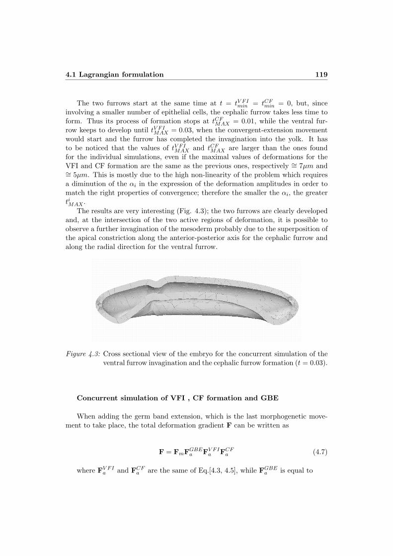
4.1 Lagrangian formulation 119
The two furrows start at the same time at t = tV FImin = tCF
min = 0, but, sinceinvolving a smaller number of epithelial cells, the cephalic furrow takes less time toform. Thus its process of formation stops at tCF
MAX = 0.01, while the ventral fur-row keeps to develop until tV FI
MAX = 0.03, when the convergent-extension movementwould start and the furrow has completed the invagination into the yolk. It hasto be noticed that the values of tV FI
MAX and tCFMAX are larger than the ones found
for the individual simulations, even if the maximal values of deformations for theVFI and CF formation are the same as the previous ones, respectively (= 7µm and(= 5µm. This is mostly due to the high non-linearity of the problem which requiresa diminution of the "i in the expression of the deformation amplitudes in order tomatch the right properties of convergence; therefore the smaller the "i, the greatertiMAX .
The results are very interesting (Fig. 4.3); the two furrows are clearly developedand, at the intersection of the two active regions of deformation, it is possible toobserve a further invagination of the mesoderm probably due to the superposition ofthe apical constriction along the anterior-posterior axis for the cephalic furrow andalong the radial direction for the ventral furrow.
Figure 4.3: Cross sectional view of the embryo for the concurrent simulation of theventral furrow invagination and the cephalic furrow formation (t = 0.03).
Concurrent simulation of VFI , CF formation and GBE
When adding the germ band extension, which is the last morphogenetic move-ment to take place, the total deformation gradient F can be written as
F = FmFGBEa FV FI
a FCFa (4.7)
where FV FIa and FCF
a are the same of Eq.[4.3, 4.5], while FGBEa is equal to

120 Chapter 4. Concurrent simulation of morphogenetic movements
FGBEa =
(1 + "GBE$ (g(t)GBE),$
GBE
,$i$(+)" i$(+)
+(1 + "GBE
z (g(t)GBE),GBEz
(1 + '$2(z)),z('$(z)ir(+) + iz)" ('$(z)ir(+) + iz)
+ n0(+, z)" n0(+, z)
(4.8)
and g(t)GBE is slightly di!erent from g(t)V FI and g(t)CF . In fact, even if inreality the GBE starts while the process of invagination of the ventral furrow is stilltaking place, here we assume that the convergent-extension movement begins oncethe VFI has completed. Thus we set tGBE
min = tV FIMAX = 0.007 while the cephalic furrow
completes its formation at tCFMAX = 0.001 and tGBE
MAX has been found at t = 0.02.
Figure 4.4: The furrows start their formation at t = 0; the cephalic furrow stops ear-lier (tCF
MAX = 0.001) and once the ventral furrow has completed formed(tV FI
MAX = tGBEmin = 0.007), the germ band begins to elongate and will stop
at t = 0.02.
As mentioned earlier, for this specific case we have assumed that the cells in-volved firstly in the ventral furrow invagination process are later interested by theconvergent-extension movement. Therefore, when superposing the relative activeregions, we obtain this time two intersection: again for the ventral and the cephalic

4.1 Lagrangian formulation 121
furrow and now also for the ventral furrows and the germ band extension (Fig. 4.5).
Figure 4.5: Ventral view of the embryo. The three active regions are represented(light green: VFI and CF, light blue: GBE); in red the relative intersec-tions.
If for the ventral and the cephalic furrows, the maximal apical constrictions foreach cell are very similar to the ones found for the previous concurrent simulation,respectively (= 5µm along the cross section and (= 4µm along z, we can not state thesame for the germ band extension. In fact for tGBE
MAX = 0.02 we obtain an elongationof about 2.5 · 10"2µm and a shortening of 2 · 10"2µm. This is probably due tothe fact that the cells in the ventral region of the embryo, that are completelyinternalized and apically deformed by now, are not able anymore to undergo thesame convergent-extension movement as observed during the individual simulation.Such peculiar aspect constitutes an important limitation for our model and it ispossible to notice it if we observe the successive phases of the simulation shown inFig. 4.6. The formation of the two furrows is clearly evident as for the individualsimulations; the GBE instead is not so pronounced, except at the posterior polewhere a beginning of a vortex movement is noticeable. Furthermore the presence ofthe cephalic furrow toward the anterior pole seems to highly inhibit the extensionof the tissues. We remark also the fact that the ventral furrow, which is supposedto stop its invagination at tV FI
MAX = 0.007, seems to keep internalizing (Fig. 4.6f),probably triggered by the convergence of the cells involved in the elongation of thegerm band.
In order to sort out such inconveniences, we propose two di!erent solutions. Thefirst one concerns the active deformation region for the GBE. So far we have consid-ered that most of the cells involved in ventral furrow invagination, are successivelydeformed by the convergent-extension movement (Fig. 4.5), however in reality suchcells, that completely internalized, later spread through the yolk so that a new tis-sue forms. Therefore it seems to us that a new population of cells, still a!ected butmore slightly by the previous elementary deformations, undergoes the extension ofthe germ band. Since it would be too di"cult to numerically simulate the closure
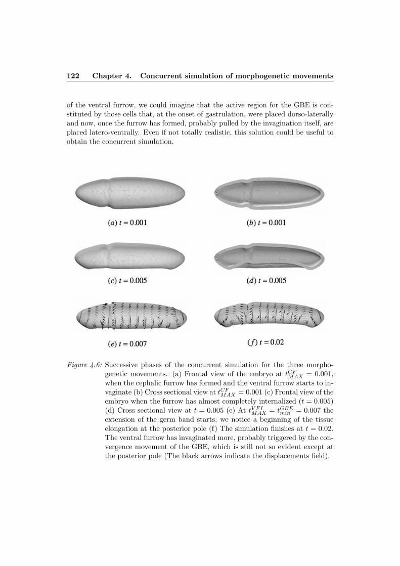
122 Chapter 4. Concurrent simulation of morphogenetic movements
of the ventral furrow, we could imagine that the active region for the GBE is con-stituted by those cells that, at the onset of gastrulation, were placed dorso-laterallyand now, once the furrow has formed, probably pulled by the invagination itself, areplaced latero-ventrally. Even if not totally realistic, this solution could be useful toobtain the concurrent simulation.
Figure 4.6: Successive phases of the concurrent simulation for the three morpho-genetic movements. (a) Frontal view of the embryo at tCF
MAX = 0.001,when the cephalic furrow has formed and the ventral furrow starts to in-vaginate (b) Cross sectional view at tCF
MAX = 0.001 (c) Frontal view of theembryo when the furrow has almost completely internalized (t = 0.005)(d) Cross sectional view at t = 0.005 (e) At tV FI
MAX = tGBEmin = 0.007 the
extension of the germ band starts; we notice a beginning of the tissueelongation at the posterior pole (f) The simulation finishes at t = 0.02.The ventral furrow has invaginated more, probably triggered by the con-vergence movement of the GBE, which is still not so evident except atthe posterior pole (The black arrows indicate the displacements field).

4.2 Updated Lagrangian formulation 123
Nevertheless, it is necessary to take into account that, when the GBE starts,the initial configuration has changed and it needs therefore to be recalculated. Fur-thermore, the initial regular geometry representing the embryo, is not an ellipsoidanymore so that the parametrical description has to be adapted. For this reasonwe propose a second solution consisting in introducing an ”updated”Lagrangian for-mulation that allows to decompose the total deformation into several intermediarysteps, so that the reference configuration is updated, as for the case of a Eulerianformulation. In the next section we are going to analyze more in detail this newapproach.
4.2 Updated Lagrangian formulation
This method is very similar to the one used by Sidoro! (Sidoro! [1976]) to definethe behaviour of a visco-elastic material. He demonstrated that the greater thenumber of the internal variables, the more accurate and rigorous the description ofa real material. The approach fits very well for our specific case since allows us tointroduce the germ band extension on a configuration modified by the formation ofthe two furrows, the ventral and the cephalic ones.
4.2.1 Kinematic description
Let us analyze the scheme proposed in Fig. 4.7. The total deformation F is decom-posed into several intermediate steps that, from the initial undeformed position pof a generic material point (as defined in Eq. [3.4]), lead to the final configurationx2 corresponding to the final shape after the three morphogenetic movements havetaken place. Practically we have two main phases:
• the first one when the elementary cell deformations triggering the formationof the two furrows are applied; the incremental parameter t runs from t0 to t1.From p we pass to x1 through F1, which can be written as
F1 = Dpx1 = Fm1Fa1 = Dx1x1Dpx1 (4.9)
with Fa1 and Fm1 the further active and the passive deformation gradientsrespectively;
• the second phase corresponds to the extension of the germ band, which isintroduced considering x1 the new reference position (here t runs from t1 tot2). So, if previously the initial configuration corresponded to p, now we havex1 = p + u1, where u1 is the displacement during the first phase. As for thefirst part, we can write
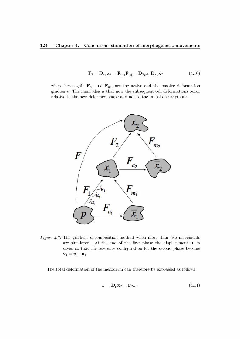
124 Chapter 4. Concurrent simulation of morphogenetic movements
F2 = Dx1x2 = Fm2Fa2 = Dx2x2Dx1 x2 (4.10)
where here again Fa2 and Fm2 are the active and the passive deformationgradients. The main idea is that now the subsequent cell deformations occurrelative to the new deformed shape and not to the initial one anymore.
Figure 4.7: The gradient decomposition method when more than two movementsare simulated. At the end of the first phase the displacement u1 issaved so that the reference configuration for the second phase becomex1 = p + u1.
The total deformation of the mesoderm can therefore be expressed as follows
F = Dpx2 = F2F1 (4.11)

4.2 Updated Lagrangian formulation 125
It has to be noticed that, in applying the elementary cell deformations, we fol-lowed the temporal succession of the events, which provides in order the formation ofthe cephalic and ventral furrows and subsequently the convergent-extension move-ment of the tissues at the germ band region. Additionally, we have again for thissimulation a multiplicative decomposition, but this time each factor itself is thecomposition of an active and a passive contributions.
First phase
We are now going to focus on the first part of the simulation. Given the consid-erations made in the previous chapter, only apical constriction is introduced alongthe section and the horizontal axis of the embryo, in order to get respectively theventral and the cephalic furrows. Any point p at the initial configuration is definedas in Eq.[3.4]; the intermediate configuration x1 can be written as
x1 = '(z1)ir(+1) + z1iz + $n1(z1, +1) (4.12)
with $ the distance between the generic point p and its projection p0 on themiddle surface (Eq. [3.2]), along the normal vector n0(+, z) (Eq. [3.5]). n1(z1, +1) isthe normal vector to the intermediate position x1 and is equal to
n1 =ir(+1)! '$(z1)iz/
1 + '$(z1)2(4.13)
+1 and z1 are defined as in Eq. [3.16] and [3.20] as follows
+1 = + + "ac(t)2$
hm(+)
z1 = z + "ceph(t)2$
hm(z)
(4.14)
where "ac(t) and "ceph(t) are the amplitudes of the elementary deformations anddepend on the evolution parameter t (see Chapter 3). Only apical constriction hasbeen implemented since we have demonstrated in Chapter 3 that it is actually theactive deformation leading to the invagination of the mesoderm for both the furrows.h is the thickness of the mesoderm and m(+) and m(z) are the periodic functions asdefined in Eq. [3.17]. The active deformation gradient Fa1 can be directly deducedfrom Eq. [3.6], so that we obtain
126 Chapter 4. Concurrent simulation of morphogenetic movements
Fa1 =
+1 + "ac(t)2'
h m$(+),,1$
,$i$
"+1
#" i$(+)
+
+1 + "ceph(t)2'
h m$(z),,1z
,z (1 + '$2(z)))'$ (z1) ir
"+1
#+ iz
*" ('$(z)ir(+) + iz)
+',1$
2"ac(t)h
m(+)i$"+1
#+ ,1z
2"ceph(t)h
m(z)"'$ (z1) ir
"+1
#+ iz
#
+n1"+1, z1
#*" n0(+, z)
(4.15)
where ,$ and ,z are the ones of Eq. [3.12], while ,1$ and ,1z are
,1$ =
4' (z1) +
$/1 + '$2 (z1)
5
,1z =
41! $'$$ (z1)
1 + '$2 (z1)(3/2)
5 (4.16)
Second phase
Once the two furrows have formed, we can implement the convergent-extensionmovement, which provides the second and final configuration of the entire systemx2. However, we have to take into account the fact that the new embryo geometrydoes not correspond to an ellipsoid anymore, therefore we consider it as a generalshell on which we apply the further elementary strains triggering the germ bandextension. In Fig. 4.8 we show the typical active deformations applied on a cell,which could be placed at the intersection of the VFI and GBE active regions, thatis therefore apically constricted at t1 along /2. Similar considerations could be donefor a cell at the intersection of the CF and GBE active regions, even if in that casethe cell would be apically constricted along /1.
Let us call x10 [/1(+), /2(z)] all the points on the deformed middle surface of themesoderm, with /1 and /2 the variables of the new system of curvilinear coordinatesand depend on + and z. Since the active deformations are still defined with respectto the middle surface, we need to calculate the ”updated” reference position of anypoint x1[/1(+), /2(z), $1($)] through the thickness of the mesoderm as follows
x1(/1, /2, $1) = x10(/1, /2) + $1n10(/
1, /2) (4.17)
where $1 is the distance between x1 and x10 along the normal n10(/1, /2) passingby x1 to the middle surface (Fig. 4.9).

4.2 Updated Lagrangian formulation 127
Figure 4.8: Convergence-extension movement on a cell that is apically constrictedalong /2.
When applying the convergence from the dorsal to the ventral region of theembryo, therefore along /2, and the extension along the anterior-posterior axis,therefore along /1, the intermediate position x2 can be expressed as
x2 = x10(/1, /2) + $1n10(/1, /2) (4.18)
where
/1 = (1 + "GBEz (t))/1
/2 = (1 + "GBE$ (t))/2
(4.19)
with, once again, "GBE$ (t) and "GBE
z (t) are the amplitudes of the active de-formations, as defined in Chapter 3. As previously mentioned, by the formationof the two furrows, the embryo is not an ellipsoid anymore; thus the expression ofthe intermediate position x2 can not correspondingly be calculated. Therefore, werather proceed in the following way. The initial middle surface is obtained by itsCAD representation (patches of Beziers surfaces) and the initial normal n0(/1, /2)is computed over it. The deformed surface at t1 is numerically obtained and itsrelative unit normal is given by

128 Chapter 4. Concurrent simulation of morphogenetic movements
Figure 4.9: Cross-sectional view of the embryo at the end of the first phase (z =0, t = t1).
n10(/1, /2) =
F"T1
)n0(/1, /2)
*
+F"T1 [n0(/1, /2)] +
(4.20)
This normal is extended through the thickness of the mesoderm at the sameposition, so that the full kinematic supplied by Eq.[4.18] can be formulated.
The active deformation gradient Fa2 in the ”updated” curvilinear system can beclassically obtained as
Fa2 =%x2
%/1"!x1/
1 +%x2
%/2"!x1/
2 +%x2
%$1"!x1$
1 (4.21)
The vectors
4.2 Updated Lagrangian formulation 129
!x1/1 =
g)2 $ g'1
g
!x1/2 =
g'1 $ g)1
g
!x1$1 =
g)1 $ g)2
g
(4.22)
form the new contravariant basis, with g defined as in Eq.[2.15]. g)1 ,g)2 ,g'1
are instead the new tangent vectors when $1 '= 0 and they are expressed as
g)1 =%x1
%/1
g)2 =%x1
%/2
g'1 =%x1
%$1
(4.23)
Actually, such tangent vectors can be expressed in function of the initial tangentvectors at t0, numerically computed in the new system of curvilinear coordinates(/1, /2, $1). Thus, they can be rewritten as follows
g)1 = F1(g0!1) = F1
%p(/1, /2, $1)%/1
g)2 = F1(g0!2) = F1
%p(/2, /2, $1)%/2
g'1 = F1(g0"1) = F1
%p(/1, /2, $1)%$1
(4.24)
and Eqs. 4.22 become
!x1/1 = F"T
1 (#p+)
!x1/2 = F"T
1 (#pz)
!x1$1 = F"T
1 (#p$)
(4.25)
4.2.2 The Principle of the Virtual Power and stress updated scheme
As already mentioned, the concurrent simulation proposed in this section is com-posed by two separated phases (Fig. 4.10):

130 Chapter 4. Concurrent simulation of morphogenetic movements
• the first one starts at t0 and stops at t1, when both the ventral and the cephalicfurrows have formed. We calculate F which corresponds here to F1;
• the second one runs from t1 to t2, when the process of convergence-extensionends. F is calculated on the deformed geometry and is the composition of F2
and F1, this last one fixed.
Figure 4.10: Successive phases of the updated concurrent simulation.
The Principle of the Virtual Power is still employed. Thus, for the first part,Eq.[2.28] defines the mechanical equilibrium of the system, with the First Piola-Kirchho! tensor "1 expressed as in Eq.[2.34]; the displacements u1 are saved sothat we are able, once the ventral and the cephalic furrows have formed at t1, toobtain the ”updated” reference position x1. Therefore, for the second part of thesimulation, not only we will apply the further active deformations on this new anddeformed initial configuration, but we will also need to take into account the stressesthat have been developed during the first phase. Since the First Piola-Kirchho!tensors "1 and "2 can not be added because defined over two configurations, wemust consider the Second Piola-Kirchho! tensors S1 and S2 that are referred toonly one configuration.
In order to do so, as similarly as for the displacements, we save at t1 the SecondPiola-Kirchho! tensor S1, which is equal to
S1 = Ja1F"1a1
Sm1F"Ta1
(4.26)
with Ja1 the determinant of Fa1 and Sm1 the Second Piola-Kirchho! tensorrelative to the intermediate configuration of the first phase. For the second phaseinstead, we have
S2 = Ja2J (Fa2F1)"1 Sm2 (Fa2F1)"T (4.27)

4.3 Conclusions 131
with Ja2 the determinant of Fa2 and Sm2 the Second Piola-Kirchho! tensorrelative to the intermediate configuration of the second phase.
Therefore "2 is still expressed as in Eq.[2.29], but this time we have
"2 = F (S1 + S2) (4.28)
It has to be noticed that, for both the first and the second phases, the boundaryconditions do not change since they are defined with respect to the very initialconfiguration; therefore their expression is the sames as in Eq.[2.28].
4.3 Conclusions
In this chapter we propose the concurrent simulation of the three morphogeneticmovements that have been individually obtained in Chapter 3.
In the first part a preliminary tentative is proposed. The method used is themost intuitive since it allows to couple the events, following their chronological suc-cession, by simply multiplying the active deformation gradients; therefore no furthermanipulations of the single formulation are required. Two simulations are shown:the first one allows to reproduce the formation of the two furrows, for the second onealso the germ band extension is introduced. If in the first case the results are consis-tent and interesting, for the second one some limitations are observed. In particular,we notice that the convergent-extension movement is not so pronounced comparedto the individual simulation; this is probably due to the fact that the cells involvedin this process have already been deformed by the elementary forces triggering theventral and the cephalic furrows. Additionally, the embryo geometry, once the twofurrows have completely formed, is not an ellipsoide anymore, thus the referenceconfiguration with respect to which the germ band extension is applied has changedtoo. A more accurate and reliable approach is necessary.
In the second part of the chapter we amply describe the theory of a new ”updated”Lagrangian formulation, which allows to take into account the two important aspectspreviously pointed out. Specifically, the total deformation is decomposed into severalsteps so that the reference configuration is constantly updated; two main phases arecontemplated. During the first one the two furrows are obtained and the analyticalformulation of the active deformation gradient directly couple together the elemen-tary forces triggering the two movements. During the second one the germ band isobserved; the initial geometry at the beginning of this phase has changed, thus anew curvilinear system is introduced and both the convergence and the extensionof the tissues are applied. Even though the results for this second essay are still inprogress, we think that the new approach represents one of the major perspectiveof the present work. Firstly because of the accuracy in the geometrical descriptionthat rarely has been so detailed; secondly because we will be able to provide a very
132 Chapter 4. Concurrent simulation of morphogenetic movements
realistic representation of part of the gastrulation process, with the most importantevents simulated. Neverthelss, the main di"culty in setting up this simulation isdue to the complexity of the several changes in shape undergone by the tissues andfurthermore by the fact that they are perfectly synchronized in the real embryo.

Chapter 5
Conclusions and perspectives
In this work we present a three dimensional finite element model of the Drosophilaembryo by which we reproduce part of the gastrulation, one of the most impor-tant phases of the developmental process. If the approach used has often beenemployed for similar studies and therefore largely known in mechanics, we think onthe other hand that the results obtained here can be considered rather original fortwo principal reasons. First of all, with a single model we are able to simulate threemorphogenetic movements that induce important shape changes of the embryonictissues; specifically ventral furrow invagination, cephalic furrow formation and germband extension. We can provide both the individual simulation of the main eventsand the concurrent simulation by two or three of them, which constitutes the mostinnovative feature of our work. Secondly, not only we have confirmed most of thehypotheses put forward by biologists, but we have also found new hints of discus-sions that may lead to new interpretations of the problem; therefore our model canbe considered a very useful tool for further analyses.
In the first chapter we have proposed a general overview of the Drosophila em-bryogenesis so that the major events are traced and the relevant aspects are pointedout. In particular we have focused on the strong connection between genetics andmechanics that has actually been observed for long time in in vivo studies. Eachone of the morphogenetic movement considered here is controlled by specific genesthat exert then an important influence on the elementary forces acting on the cells.Only recently also the inverse process has been detected; it seems in fact that acertain number of mechanical deformations occurring to the tissues may favour theexpression of genes at di!erent spots than the usual ones. However, it is still unclearhow the mechanical stimuli are transformed into chemical signals, so that such phe-nomenon, better known as mechanotransduction, remains enigmatic. In this sectionof the work we also provide a brief review on previous works that have been foundin literature. Most of them allow to reproduce the invagination of the ventral furrowand the convergent-extension of the cells, while, to the best of our knowledge, none
133

134 Chapter 5. Conclusions and perspectives
consents to simulate the formation of the cephalic furrow that is instead presentedhere. The first models are constituted of structural elements, usually trusses or bars,that play the role of actuators to reproduce the cytoskeleton components (i.e. mi-crotubules and microfilaments). In despite of this, many of them do not take intoaccount external components to the epithelial layer such as the yolk, which fills theinternal cavity, and the vitelline membrane that surrounds the embryo. This is theirmain drawback since the absence of one or both of these components may engenderfinal configurations that do not match with experimental observations. Also it hasto be noticed that the embryo has often been represented in a two dimensional spacewhich does not assure a realistic reproduction of the biological system. Few recentworks provide three dimensional models of ventral furrow invagination; the embryois described as a continuum on which the active and the passive forces acting on thecells, that are strongly related, are applied. So far then, the models are specific toa single event, while here we show how the analytical formulation can be modifiedand adapted so that more than one movement can be simulated.
A gradient decomposition method is used and it is exhaustively described in thesecond chapter. This method allows to take into account both the active and thepassive contributions; the former corresponds to the natural tendency of the cellsto deform as if they were completely free, which can lead to geometrical incompat-ibilities. Therefore the latter occurs, a consequent response of the tissues in orderto guarantee the continuity of the system. Di!erent interpretations of the approachcan be contemplated, as amply discussed in this section; in particular we proposea comparison with an equivalent thermal dilatation and we analyze the potentiale!ects of the local active forces on both the active and passive domains and in par-ticular at the internal and external cellular interfaces. The mechanical equilibriumis expressed by the Principle of the Virtual Power so that the internal forces areincluded together with the yolk pressure and the contact between the mesodermand the vitelline membrane. We have also treated here the choice of the mate-rial describing the mesoderm, which is assumed to constitute the most part of theembryonic tissues. Given the very few information about the mechanical charac-teristics required here, that are often di"cult to detect, we have opted for a linearSaint-Venant constitutive law, which does not take into account the non linearitiesengendered by the visco-elastic properties of the embryonic tissues, but may be any-way a useful tool for a first qualitative analysis of the problem. Nevertheless, awareof such limitations, we have compared our model to the Hyperelastic one, which hasnormally been employed in previous studies.
Chapter three focuses on the analysis of each morphogenetic movement andthe relative results. In the first part we describe how the analytical expressionsof the active deformation gradients are obtained, according to the elementary celldeformations introduced. Such formulations, coupled with the passive gradients, willbe implemented in the Principle of the Virtual Power, together with the boundaryconditions of the system, in order to get the final tissues deformation. In the second
135
part of the chapter we analyze the results for each morphogenetic movement; for thethree events the agreement with the experimental observations is rather consistent,thus most of the hypotheses made by biologists are confirmed. Additionally we havebeen able to put forward some new aspects which may lead to interesting conclusionsand therefore further hints of discussion. Here we resume the major remarks thatcan be deduced from the numerical simulations:
• first of all, a parametrical study has been conducted for the ventral furrow,which has pointed out the influence exerted by some variables such as thesize of the active deformation region and the dimensions of the material cells.In particular we have observed that, when let varying these parameters, theinvagination is almost the same for all the cases, while the phenomenon of theself-contact between the two strips of the mesoderm may be evidently inhibitedor enhanced;
• by manipulations on mutants, biologists have individuated only two activeforces leading to ventral furrow invagination: apical constriction and apico-basal elongation. Although, for our simulation, we have first implemented onlythe former and the invagination of the mesoderm still occurs; this allows us toconclude that probably apical constriction is actually the only responsible ofthe entire process of invagination, while apico-basal elongation, together withthe other three elementary deformations detected, are passive responses of thecells. This hypothesis has been also confirmed through the simulation of thecephalic furrow, for which again only apical constriction has been introducedand, even if a small number of cells is involved, the invagination takes place;
• for the germ band extension, the final displacements found for our simulationreproduce pretty well the real convergence-extension of the tissues; in particu-lar we have observed the vortex movements at the anterior and posterior poles,as in the real embryo. Also we have compared the velocity field with exper-imental data available in literature and they present almost the same trendthrough the embryo;
• the Hyperelastic constitutive law, amply discussed in the second chapter, hasbeen tested for the simulation of the germ band extension. The results arenot so di!erent from the ones obtained with the Saint-Venant model used alllong our analysis, which confirms that our first choice, even if presenting somelimitations, can anyway be considered appropriate for the present work;
• we have estimated the induced forces, specifically pressures and shear stresses,that may develop through the embryo when the three morphogenetic move-ments take place. These forces can be compared to the usual ones applied oncells placed in a bioreactor over 24h that may engender several cellular activ-ities such as migration, proliferation or adhesion. Most importantly, for the
136 Chapter 5. Conclusions and perspectives
specific case of the germ band extension we have found that the convergent-extension movement of the tissues actually leads to a compression at the an-terior pole which triggers, as observed during experiments, the expression ofthe gene twist, normally expressed at the ventral region of the embryo. Thisresult could confirm the presence of a mechanotransduction pattern by which amechanical stimuli is transformed into a chemical signal, even at long distance;
• finally, aware that the geometry of our model is a simplification of the realembryo, we have conducted an interesting analysis to evaluate how the varia-tion of the curvature radius may a!ect the final configuration during ventralfurrow invagination and germ band extension. So far three geometries havebeen tested and other two are in progress in order to take into account twoimportant aspects: the non symmetry with respect to the vertical axis of theembryo, which provides a more rounded posterior pole, and the flattening ofthe dorsal region.
Given the consistence of the results for the individual simulations of the threemorphogenetic movements, we have decided to perform the concurrent simulationof the events, which is the object of the fourth chapter. A preliminary essay is pre-sented which provides a consistent final configuration for the simulation of the twofurrows, but some limitations are observed when the germ band extension is intro-duced. Therefore a second method, more closely related to the observed successionof movements, is proposed. It allows to take into account several peculiar aspects sofar put aside, that may instead play a significant role in the global response of theembryo. Even though the results for this second simulation are still in progress andthus not presented here, we think that this part of the work represent one majorcontribution of the present study, thus an interesting perspective to pursue.
The mechanical properties of the mesoderm and sensibility analysis
During development the thin tissues composing the embryo undergo severalmovements and deformations that are crucial to normal morphogenesis. Thus, itis very important to know the mechanical properties of the embryonic structureswhich unfortunately so far, compared to orthopaedic or cardiac mechanics, havebeen very di"cult to detect. Actually, if many progresses have been made for mea-suring the mechanical characteristics of individual cells and bulk tissues, still littlehas been done to improve methods allowing to obtain information from specimensof embryonic epithelium. These data play a significant role in biomechanics and es-pecially in embryogenesis, where materials can exhibit elastic, visco-elastic, viscousor plastic properties and the consequences of these di!erences may be substantialfor morphogenetic movements. Our model, as many among the previous ones, isbased on several approximations concerning such properties, so that its validationmay appear uncertain. Therefore, in order to refine this key aspect so far rarely

137
explored in numerical simulations, we would like to introduce a visco-elastic modelto describe the mesoderm, which must then be supported by experimental observa-tions. Nonetheless, if on one hand it is essential to determine the right mechanicalcharacteristics of the tissues in order to obtain consistent results, on the other itwould be equally interesting to perform a sensibility analysis, which will allow toevaluate the influence of specific parameters, such as the Young’s modulus, on thefinal configurations relative to each morphogenetic movement.
Cephalic furrow simulation
For the cephalic furrow simulation a few simplifications have been made. Actu-ally, by experimental movies, it has been observed that the furrow starts vertically,at about 60% of the horizontal length of the embryo, but, throughout its forma-tion, it is pushed, probably triggered by the extension of the germ band, toward theanterior pole. Thus, at the final configuration, once the cells in the active regionhave completely internalized, the furrow is inclined at about 30! with respect to thedorsal-ventral axis; the cells apically constrict and simultaneously skew, so that theircurvilinear coordinate + changes too. For the present work we have decided to modelthe furrow parallel to the vertical axis of the embryo, without taking into account itsmovement during the invagination process. The next step would be to implement anEulerian formulation which will provide the expression of the intermediate positionx that will include both the deformation of the cells along the cross section and thedisplacement of the tissues associated to a determined velocity.
From the embryo to the single cell
In the present work, the mesoderm is represented as a continuum on which theelementary forces, that trigger the di!erent morphogenetic movements, are applied.We use then a macro-scale approach of the problem, whereas the active deformationsinvolve the membranes of the cells that compose the embryonic tissue at a micro-scalelevel. Nevertheless our model provides the useful tools to perform a more detailedanalysis, where each cell will be described including some of its essential componentssuch as the nucleus, the micro filaments and other elements of the cytoskeleton. Inthis way, we will be able to test also other types of strain, such pressure and shearstress, to which cells in culture or bioreactor are usually submitted to.

138 Chapter 5. Conclusions and perspectives
Appendix A
Large deformation theory
All biological tissue can in general undergo large deformation in physiological activ-ity. Large deformation is typically defined as anything greater 3 to 5 % strain. Whenthe deformation is small, we can use the small deformation linear strain tensor andthe Cauchy stress tensor. However, once deformations exceed 5% strain, we mustuse the appropriate stress and strain tensor, constitutive relations that account forlarge deformations.
A.1 The deformation gradient tensor
The first step in defining large deformation strain measures is to determine the rela-tionship between what is known as the reference, initial or undeformed configurationand the deformed configuration of a body. The reference, initial or undeformed con-figuration is the condition of the body in a 3D space before loads and constraintshave been applied to it. The deformed configuration is the location and the shape ofthe body after loads have been applied to it. Obviously the body can undergo rigidbody motions in addition to strain when loads are applied to it. An illustration ofthe relationship between the initial and deformed configuration is shown below.
We defined two di!erent vectors: one in the reference configuration p and onefor the deformed configuration x. The relationship between the two position vectorsis the displacement vector.
By vector addition, we can directly write the equation defining it:
x = p + u (A.1)
If we consider the vectors describing material orientation in each configuration,these vectors essentially describe an infinitesimal piece of material of the body. Wewill note these vectors as dp in the reference configuration and dx in the deformedconfiguration and so, applying the chain rule, we obtain a mapping between the
139
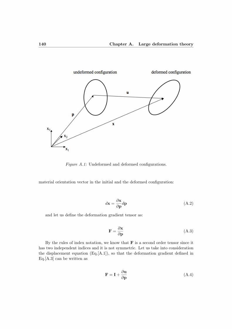
140 Chapter A. Large deformation theory
Figure A.1: Undeformed and deformed configurations.
material orientation vector in the initial and the deformed configuration:
dx =%x%p
dp (A.2)
and let us define the deformation gradient tensor as:
F =%x%p
(A.3)
By the rules of index notation, we know that F is a second order tensor since ithas two independent indices and it is not symmetric. Let us take into considerationthe displacement equation (Eq.[A.1]), so that the deformation gradient defined inEq.[A.3] can be written as
F = I +%u%p
(A.4)

A.2 Strain and deformation measures 141
Because F is a one to one mapping from the undeformed to the deformed con-figuration, then the inverse mapping must exists (F"1). The following relationshipsinvolving F are useful since they allow us to map the area and the volume betweenthe undeformed and the deformed configurations. If we map a volume, using the3rd invariant or determinant of the deformation gradient tensor, we have:
dVx = detFV = JdV (A.5)
For the area, considering the drawings of area change given in Fig. A.2.
Figure A.2: Di!erential area element before and after deformation.
The mapping between the two configurations is (Smith [1993], Taber [2004]):
nx dSx = J F"Tn dS (A.6)
A.2 Strain and deformation measures
Although the deformation gradient tensor defined above is one measure of how abody changes under load, it cannot be used directly for strain characterization be-cause it contains rigid body motions. To define a strain measure, we will try to
142 Chapter A. Large deformation theory
measure the change in length squared in a material vector in going from the initialconfiguration to the deformed configuration and these measures should be indepen-dent of rigid body rotation. For the reference configuration, the length squared of avector can be merely written as the dot product with itself:
(dS)2 = dl dl (A.7)
and the same for the deformed configuration:
(dSx)2 = dlx dlx (A.8)
A strain measure should be a mapping that tell us how much a piece of materialis squeezed when going from one to the other configuration, specifically how lengthand angle change. Thus for a strain tensor E we write:
(dSx)2 ! (dS)2 = dlxdlx ! dl dl = 2 dpE dp (A.9)
where
E =12(FTF! I) (A.10)
We have not made any assumptions about the magnitude of the deformation,so the strain tensor given above is exact for any size deformation and it is knownas the Green-Lagrange strain tensor. An often used quantity to define constitutiveequations for large deformations, is the Right Cauchy deformation tensor:
C = FTF (A.11)
substituting this in Eq.[A.10] we have:
E =12(C! I) (A.12)
This tensor is symmetric and positive definite.
A.3 Large deformation stress measures 143
A.3 Large deformation stress measures
We must now define new stress measures and they have to be appropriate whencoupled with the strain measures that we have defined in the previous section. Wehave already encountered one stress measure, the Cauchy stress tensor; this stressis basically defined as force on unit deformed area. The problem with using theCauchy stress tensor for analyzing materials undergoing large deformation is thatwe generally do not know the area in the deformed configuration, thus we need todefine a stress measure that we can use in the reference configuration. The firstprinciple used when trying to derive a stress tensor with respect to the referenceconfiguration is that the stress tensor in the reference configuration area should givethe same force as the Cauchy stress tensor defined in the deformed configuration.Recalling that the traction is a force on a surface and is the product of the stressand the normal vector to the surface, we can define the total force in the deformedconfiguration as:
dPx = ! nxdSx (A.13)
where dPx is the total force, ! is the Cauchy stress tensor, nx is the normalvector to the surface of the deformed configuration, and dSx is the surface area inthe deformed configuration. Noting that we would like the same force developed bythe new stress tensor, T, in the reference configuration with normal n and area dSx,we define:
dPx = " n dS (A.14)
where " is then the 1st Piola-Kircho! stress tensor. Now recalling the mappingbetween reference and deformed configuration surface areas, we can write the defi-nition of the force in the deformed configuration as:
" ndS = ! nx dSx = !J F"T n dS (A.15)
Now that we have the expressions for the total force consistent in terms of thenormal and area, we can substract the two expressions and set the result equal tozero, so that we obtain:
" = J !F"T (A.16)
144 Chapter A. Large deformation theory
therefore the 1st Piola-Kircho! stress gives us the actual force rendered in theundeformed surface area.
The 1st Piola-Kircho! stress tensor is not symmetric; this makes it more di"cultto use with numerical analyses like the finite element method. Furthermore, it is notdirectly relied to E, thus we need to look further for an appropriate stress tensor. Anadditional step we can take is not to derive a stress tensor based on the force dPx inthe deformed configuration, but rather map the force dPx back into the undeformedconfiguration using the inverse of the deformation gradient tensor. Doing this weobtain:
dP = F"1dPx (A.17)
if we define another stress tensor, S, which gives the total force on the area inthe undeformed configuration, we obtain:
dP = Sn dS (A.18)
then
dP = F"1! J F"Tn dS (A.19)
Now we can compare the third stress tensor S, which is the 2nd Piola-Kircho!stress tensor, to the Cauchy stress tensor as:
S = J F"1! F"T (A.20)
The number of indices and di!erent stress tensors being thrown around canbe quite confusing; the deformation gradient maps forward to the deformed con-figuration, while the inverse deformation gradient maps backwards to the initialconfiguration.
One di"culty with all these stress tensors is how to envision their physical mean-ing. In truth, the physical meaning of the 2nd PK stress is hard to interpret. Itis mainly used as a vehicle to get what is called an objective constitutive equation,after which the Cauchy stress is computed from the 2nd PK stress.

Appendix B
Mechanics of growing mass
When talking about tissues, one must distinguish between hard tissues, such asbones and teeth, and soft tissues, such as blood vessels, tendons and ligaments. Incontrast with hard tissues, that usually undergo only small deformations and growby simple deposition on a surface, soft tissues can experience large deformations (seeAppendix A) and their growth and remodeling take place during the normal processof growth, healing process or pathological conditions (Asaro and Lubarda [2006]).Generally, the changing processes of a tissue are due to the use of the tissue itself.For instance a cyclical stress leads to the formation of a new bone, while the highblood pressure enhances the remodeling of the heart to obviate the hyperthropy.Therefore, by remodeling and modifying their structure, tissues adapt themself tothe loading conditions they are a!ected to. Taber (Taber [1995]) and Humphrey(Humphrey [1995]) both analyzed the biomechanical aspects of growth, defined asa change in volume, remodeling, a change in properties, and morphogenesis, anisovolumic change in shape and they concluded that the three processes are clearlycorrelated and overlapped.
To study the growth in plants and animals, many mathematical descriptionshave been proposed (see review Taber [1995]), most of which provide an analysisof the problem from a kinematic point of view. It has been observed that, if thegrowth strains of each element of an unloaded body are geometrically compatible,then the body remains stress-free after the growth occurs. On the other hand whenthe growth strains are incompatible, a residual stress is generated and it remainsafter all external loads are removed. Even if in the last decades the residual stresshas been largely studied, it is still not clear the purpose of its existence; the mainhypothesis is that it could assure a more uniform distribution of the loads throughthe tissue so that the global structure can better tolerate them. There are essentiallytwo types of growth: the surface growth, which occurs without generation of residualstress and by adding or resorption at a surface and the volumetric growth, which isvery similar to thermal expansion.
145

146 Chapter B. Mechanics of growing mass
B.1 Surface growth
This type of growth usually involves bones, shells, horns and branches. Let usconsider this time a surface S0 including two material regions R1 and R2 on eachside (Fig. B.1a). Each point of the domain can be located by the surface coordinates#& with " = 1, 2. At the initial time t = 0, the surface grows from both of its side sothat two new regions come to form, R3 and R4 (Fig. B.1b), that push R1 and R2
outward and are separated from them by surfaces S1 and S2.
Figure B.1: Geometry for the surface growth of a mass (modified from Taber [1995]).
At t = 0, each point is located by x0, but when growth process starts, each pointon the surface S0 generates an infinite number of particle in the new regions R3 andR4. An additional time variable ! is introduced in order to skip out the redundancyof the material coordinates; this new variable provides the time at which each particlehas formed so that we can write
x = x(#&, !, t) (B.1)
with 0 < ! < t. The new surfaces S1 and S2 can be considered the first ones ofthe new material configuration, so that their points are defined by x(#&, 0, t), whilst

B.2 Volumetric growth 147
the position of S0 at any time is x(#&, t, t). Therefore, the velocities can be writtenrespectively
v0 = x0(#&, t) for a point on S0 (B.2)v = x(#&, !, t) for a point on R3 and R4 (B.3)
The velocity v adjacent to S0 might di!er from the surface velocity v0 becauseof the relative growth velocity, which is
vg = v! v0 (B.4)
According to the side of S0 we are considering, the normal component of vg tothis surface can be either positive in a case of accretion or negative in a case ofresorption.
B.2 Volumetric growth
In the case of volumetric growth, for linear elastic problems, it is possible to super-pose the growth stresses, but in non-linear problems it is necessary to use anotherapproach. The strains measured for each material element are referring to the cur-rent zero-stress configuration, which changes according to the growth of the element.Other than the specific case of Drosophila embryo the deformation gradient decom-position method was first used in 1969 by Lee (Lee [1969]). He applied the methodfor elastic-plastic deformations occurring when both components of strain are fi-nite; doing so, the kinematics are modified to include finite elastic and plastic straincomponents. Particularly, he introduced two coupled thermodynamic systems: onecompromising termo-elasticity at finite strain and the other the irreversible pro-cess of dissipation and absorption of plastic work. For what concerns biomechanics,Rodriguez (Rodriguez et al. [1994]) studied cardiac hypertrophy during which al-terations in wall stress arising from changes in mechanical loading lead to cardiacgrowth and remodeling. To describe the shape change undergone by an unloadedtissue during growth, he introduced a mapping decomposed into two deformations.The first one indicates the local zero-stress reference state, while the second one isthe accompanying elastic transformation that ensures the compatibility of the totaldeformation. Also Taber (Taber and Perucchio [2000]) used this approach for theanalysis of growth, remodeling and morphogenesis of cardiac development. Thismethod is very similar to the one used for the present work, thus in this section wedescribe it more precisely (for further details please refer to Taber [1995]).
Let us consider a body B, which at time t0 is free stress (Fig. B.2); the body isconstituted by infinitesimal elements that undergo volumetric growth and that, after

148 Chapter B. Mechanics of growing mass
growing, remain stress free. These particular deformations may not be geometricallycompatible; thus the elements of B(t1) must be deformed again in order to makethem fit together. Therefore three deformation gradients have to be taken intoaccount:
• the growth deformation gradient Fg, which can be deduced by experiments ;
• the elastic deformation gradient Fe, which allows to maintain the integrity ofthe body and cause the presence of a residual stress !0;
• the external deformation gradient Fl.
Figure B.2: Successive configurations for a growing mass (modified from Taber[1995]).
This is a case of a Lagrangian description where a reference configuration (B(t0))is chosen and it is not changing through the time. Once the growth completedinstead, B
!(t1) can be used as reference for the loading step. The total deformationgradient can be finally expressed as follows
F = FlFeFg (B.5)

B.2 Volumetric growth 149
For what concerns the stresses, two of them are particularly interesting: theresidual stress !0, associated to the B
!(t1) configuration, and the total stress !in b(t). To find the residual stress it is necessary that F = FeFg with Fl = Iand traction-free boundary conditions. A similar approach can be used for ! butthis time Fl '= I and the boundary conditions are inhomogeneous. It has to benotice that the growth is not isovolumic trough the time, therefore detFg '= 1,specifically detFg > 1 when there is addition of volume and detFg < 1 whenremotion occurs. Finally if the material is incompressible, except for the growth,then we have Fle = FlFe.
The previous analysis takes into account the e!ects of growth on stress, butthe inverse process must be considered to know how stress influences growth. Sofar, even if experimental data pointed out how stress, strain or strain energy canmodulate growth, it is not well understood which one of this quantity play the mostsignificant role. However it is possible to write a constitutive relation of a stress-dependent growth as follows
Fg = Fg(!) (B.6)
where ! is an implicit fonction of the time. There is another form of the priorequation
Fg = Fg(!) (B.7)
which results to be more accurate from a physiological point of view since it hasbeen demonstrated that the higher the magnitude of the applied stress, the higherthe growth rate. A rigid-body rotational term is included in Fg, but it might nota!ect the stresses and can be directly reassembled into the deformation provided byFle.
The growth rate of deformation tensor can be obtained, once Fg and Fg havebeen determined, from (Rodriguez et al. [1994])
Dg =12
-FgF"1
g + F"Tg F
Tg
.(B.8)
where dot indicates the partial di!erentiation with respect to the time t. Fur-thermore the rate of volumetric growth can be expressed as
1V
dV
dt= tr Dg (B.9)
with V the growth volume.

150 Chapter B. Mechanics of growing mass
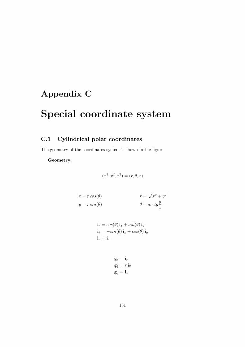
Appendix C
Special coordinate system
C.1 Cylindrical polar coordinates
The geometry of the coordinates system is shown in the figure
Geometry:
(x1, x2, x3) = (r, +, z)
x = r cos(+) r =/
x2 + y2
y = r sin(+) + = arctgy
x
ir = cos(+) ix + sin(+) iyi$ = !sin(+) ix + cos(+) iyiz = iz
gr = irg$ = r i$gz = iz
151

152 Chapter C. Special coordinate system
Figure C.1: Cylindrical polar coordinates.
Di!erential operator:
! =%
%rir +
1r
%
%+i$ +
%
%ziz
Deformation gradient:
Fii,ij =
=
>"r"R
1R
"r""
"z"Z
r "$"R
rR
"$"" r "$
"Z"z"R
1R
"z""
"z"Z
?
@
where (R,$, Z) are the cylindrical coordinates in the reference configuration.

C.2 Spherical polar coordinates 153
C.2 Spherical polar coordinates
The geometry of the coordinates system is shown in the figure
Figure C.2: Spherical polar coordinates.
Geometry:
(x1, x2, x3) = (r, +,,)
x = r sin(+)cos(,)y = r sin(+)sin(,)z = r cos(+)

154 Chapter C. Special coordinate system
g1 = ixsin(+)cos(,) + iysin(+)sin(,) + izcos(+) = irg2 = r(ixcos(+)cos(,) + iycos(+)sin(,)! izsin(+)) = ri$g3 = r sin(+)(!ixsin(,) + iycos(,)) = r sin(+)i%
Di!erential operator:
! = ir%
%r+ i$
1r
%
%++ i%
1r sin(+)
%
%,
Deformation gradient:
Fii,ij =
=
>"r"R
1R
"r""
1R sin"
"r"#
r "$"R
rR
"$""
rR sin"
"$"#
r sin(+) "%"R
r sin($)R
"%""
r sin($)R sin"
"%"#
?
@

Bibliography
M.D. Adams, S.E. Celniker, and R.A. Holt et al. The genome sequence of DrosophilaMelanogaster. Science, 287:2185–95, 2000.
R. Allena, A.-S. Mouronval, E. Farge, and D. Aubry. Concurrent simulation ofmorphogenetic movements in Drosophila embryo. IFMBE Proceedings, SpringerBerlin Heidelberg, 287:1829–1832, 2008.
R.J. Asaro and V.A. Lubarda. Mechanics of solids and materials. Cambridge, 2006.
K. Barrett, M. Leptin, and J. Settleman. The Rho GTPase and a putative RhoGEFmediate a signaling pathway for the cell shape changes in drosophila gastrulation.Cell, 91:905–915, 1997.
L.V. Beloussov. The dynamic architecture of a developing organism: an interdisci-plinary approach to the development of organisms. Kluwer, Dordrecht, 1998.
L.V. Beloussov and V.I. Grabovsky. Information about a form (on the dynamic lawsof morphogenesis). BioSystems, 87:204–214, 2007.
L.V. Beloussov and A.V. Lakirev. Generative rules for the morphogenesis of epithe-lial tubes. J. Theor. Biol., 152:455–468, 1991.
T. Belytschko, W.G. Liu, and B. Moran. Non linear finite elements for continuaand structures. Wiley, 2000.
G.W. Brodland and D.A. Clausi. Mechanical evaluation of theories of neurulationusing computer simulations. Development, 118:1013–1023, 1993.
E. Brouzes and E. Farge. Interplay of mechanical deformation and patterned geneexpression in developing embryos. Curr. Opin. Genet. Dev., 14:367–74, 2004.
J.A. Campos-Ortega and V. Hartenstein. The embryonic development of DrosophilaMelanogaster. Springer-Verlag, 1985.
V. Conte, J. Munoz, and M. Miodownik. A 3D finite element model of ventral furrowinvagination in the Drosophila Melanogaster embryo. Journal of the mechanicalbehavior of biomedical materials, 1:188–198, 2008.
155

156 Bibliography
M. Costa, D. Sweeton, and E. Wieschaus. How do Sea Urchins invaginate? usingbiomechanics to distinguish between mechanisms of primary invagination. Devel-opment, 121:425–465, 1993.
L. Davidson, M.A. Koehl, R. Keller, and G.F. Oster. How do sea urchins invaginate?using biomechanics to distinguish between mechanisms of primary invagination.Development, 121:2005–2018, 1995.
L. Davidson, G.F. Oster, R.E. Keller, and M.A.R. Koehl. Measurements of me-chanical properties of the blastula wall reveal which hypothesized mechanisms ofprimary invagination are physically plausible in the Sea Urchin stronglylocentro-tus purpuratus. Dev Biol, 209:221–238, 1999.
J.A. Davies. Mechanism of morphogenesis: the creation of biological form. ElsevierAcademic Press, 2005.
N. Desprat, W. Supatto, P.A. Pouille, E. Beaurepaire, and E. Farge. Tissue defor-mation modulates twist expression to determine anterior midgut di!erentiation inDrosophila embryos. Developmental cell, 15:470–477, 2008.
C. Nusslein-Volhard E. Wieschaus and H. Kluding. Kruppel, a gene whose activityis required early in the zygotic genome for normal embryonic segmentation. DevBiol, 104:172–186, 1984.
E. Farge. Mechanical induction of Twist in the Drosophila foregut/stomodeal pri-mordium. Curr. Biol., 13:1365–1377, 2003.
V.E. Foe, G.M. Odell, and B.A. Edgar. Mitosis and morphogenesis in the Drosophilaembryo: point and counterpoint. The development of Drosophila Melanogaster,pages 149–300, 1993.
G. Forgacs and S.A Newman. Biological physics of the developing embryo. CambridgeUniversity press, 2006.
G. Forgacs, R.A. Foty, Y. Shafrir, and M.S. Steinberg. Viscoelastic properties ofliving embryonic tissues: a quantitative study. Biophys, 74:2227–2234, 1998.
H.G. Frohnhofer and C. Nusslein-Volhard. Organization of anterior pattern in theDrosophila embryo by the maternal gene Bicoid. Nature, 324:120–125, 1986.
A. Gierer. Physical aspects of tissue evagination and biological form. Q. Rev.Biophys., 10:529–593, 1977.
J. Hardin and L.Y. Cheng. The mechanisms and mechanics of archenteron elongationduring Sea Urchin gastrulation. Dev. Biol., 115:490–511, 1986.
Bibliography 157
G.A. Holzapfel. Non linear solid mechanics. A continuum approach for engineers. JWiley Sons Ltd, 2000.
J.D. Humphrey. Mechanics of the arterial wall: review and directions. Criticalreviews in Biomed. Eng., 23:1–162, 1995.
K.D. Irvine and E. Wieschaus. Cell intercalation during Drosophila germ bandextension and its regulation by pair-rule segmentation genes. Development, 120:827–41, 1994.
A.G. Jacobson. Computer modeling of morphogenesis. Am. Zool., 20:669–677, 1980.
A.G. Jacobson and R. Gordon. Change in the shape of the developing vertebratenervous system analyzed experimentally, mathematically and by computer simu-lation. J. Exp. Zool., 197:191–246, 1976.
A.G. Jacobson, G.F. Oster, G.M. Odell, and L.Y. Cheng. Neurulation and corticaltractor model for epithelial folding. J. Embryol. Exp. Morph., 96:19–49, 1986.
R. Keller. The celular basis of epiboly: a SEM study of deep cell rearrangementduring gastrulation in Xenopus Laevis. J. Embryol. Exp. Morphol., 60:201–234,1980.
R. Keller and P. Tibbetts. Mediolateral cell intercalation in the dorsal axial meso-derm in the Xenopus Laevis. Dev. Biol., 131:539–549, 1989.
R. Keller, J. Shih, and P. Wilson. Cell motility, control and function of conver-gence and extension during gastrulation of Xenofus. In Gastrulation: movements,patterns and molecules. Plenum, 1991a.
R. Keller, J. Shih, P. Wilson, and A. Sater. Pattern and function of cell motilityand cell interactions during convergence and extension in Xenofus. In 49th Sym-posium of the Society for Developmental Biology: cell-cell interactions in earlydevelopment. J Wiley Sons Ltd, 1991b.
R. Keller, L. Davidson, A. Edlund, T. Elul, M. Ezin, D. Shook, and P. Skoglund.Mechanisms of convergence and extension by cell intercalation. Philos. Trans. R.Soc. Lond. B. Biol. Sci., 355:1399, 2000.
R. Keller, L.A. Davidson, and D.R. Shook. How we are shaped: the biomechanicsof gastrulation. Development, 71:171–205, 2003.
C. Kimmel, R. Warga, and R. Kane. Cell cycles and clonal strings during formationof the Zebrafish central nervous system. Development, 120:265–276, 1994.

158 Bibliography
V. Kolsch, T. Seher, G.J. Fernandes-Ballester, G.J. Serrano, and M. Leptin. Con-trol of Drosophila gastrulation by apical localization of adherens junctions andRhoGEF2. Science, 132:384–6, 2007.
T. Lecuit and P.-F. Lenne. Cell surface mechanics and the control of cell shape,tissue patterns and morphogenesis. Nature reviews, 8:633–643, 2007.
E.H. Lee. Elastic-plastic deformation at finite strains. J of Applied Mechanics, 36:6, 1969.
A. LeMoigne and J. Foucrier. Biologie du developpement. Dunod, 2004.
M. Leptin. Drosophila gastrulation: from pattern formation to morphogenesis.Annu. Rev. Cell Dev., 11:189–212, 1995.
M. Leptin. Gastrulation in Drosophila: the logic and the cellular mechanisms.EMBO J, 18:3187–3192, 1999.
M. Leptin and B. Grunewald. Cell shape changes during gastrulation in Drosophila.Development, 110:73–84, 1990.
J.E. Mitthenthal. The shaping of shell sheets: an application of mechanics in devel-opmental biology. Biomechanics of cell divisions, pages 327–346, 1987.
A.S. Mouronval, R. Allena, and D. Aubry. Simulations numeriques des mouvementsmorphogenetiques dans l’embryon de Drosophile: influence de la geometrie initiale.Proceedings of 9eme Colloque National en calcul de structures, Giens, 25-29 Mai,2009.
J. Munoz and G. Jelenic. Sliding contact conditions using the master-slave approachwith application on the geometracally non-linear beams. Int. J. Solids Struct, 41:6963–6992, 2004.
J. Munoz, K. Barrett, and M. Miodownik. A deformation gradient decompositionmethod for the analysis of the mechanics of morphogenesis. Journal of Biome-chanics, 40:1372–1380, 2007.
A. Nicolas, B. Geiger, and S. A. Safran. Cell mechanosensitivity controls theanisotropy of focal adhesions. PNAS, 101:12520–12525, 2004.
H. Oda and S. Tsukita. Real-time imaging of cell-cell adherens junctions reveals thatDrosophila mesoderm invagination begins with two phases of apical constrictionof cells. Journal of cell science, 114:493–501, 2000.
G.M. Odell, G. Oster, O. Alberch, and P. Burnside. The mechanical basis of mor-phogenesis. I. Epithelial folding and invagination. Dev. Biology, 85:446–462, 1981.
Bibliography 159
S. Osher and R. Fedkiw. Level set method and dynamic implicit surfaces. Springer,2003.
G.F. Oster and O. Alberch. Evolution and bifurcation of developmental programs.Evolution, 36:444–459, 1982.
PA. Pouille and E. Farge. Hydrodynamic simulation of multicellular embryo invagi-nation. Physical biology, 5:015005, 2008.
A. Ramasubramanian and L.A. Taber. Computational modelling of morphogenesisregulated by mechanical feedback. Biomechan. Model. Mechanobiol., 7:77–91,2006.
L.T. Reiter. A systematic analysis of human disease-associated gene sequences inDrosophila Melanogaster. Genome Res, 11(6):1114–25, 2001.
E.K. Rodriguez, A. Hoger, and A.D. McCulloch. Stress-dependent finite growth insoft elastic tissues. Journal of Biomechanics, 27:455–467, 1994.
S. Roth. Gastrulation in other insects. Cold Spring Harbor Laboratory Press, 2004.
G.C. Schoenwolf and I. Alvarez. Roles of neuroepithelial cell rearrangement anddivision shaping of the avian neural plate. Development, 106:427–439, 1989.
J.A. Sethian. Level set method. Cambridge University Press, 1996.
F. Sidoro!. Variables internes en viscoelasticite. milieux avec plusieurs configurationsintermediaires. Journal de mecanique, 15, 1976.
D. Smith. An introduction to continuum mechanics. Kluwer Academic Publisher,1993.
W. Supatto. Imagerie multiphoton quantitative et ablation laser par impulsions fem-tosecondes pour l’etude de l’expression genetique mecano-sensible chez l’embryonde Drosophile sauvage. PhD thesis, Institut Curie Laboratoire Physico-Chimie,2005.
W. Supatto, D. Debarre, B. Moulia, E. Brouzes, J.-L. Martin, and E. Farge. In vivomodulation of morphogenetic movements in drosophila embryos with femtosecondlaser pulses. PNAS, 102:1047–1052, 2005.
D. Sweeton, S. Parks, M. Costa, and E.Wieschaus. Gastrulation in Drosophila: theformation of the ventral furrow and posterior midgut invaginations. Development,112:775–789, 1991.
L.A. Taber. Biomechanics of growth, remodeling and morphogenesis. Appl. Mech.Rev., 48(8):487–545, 1995.
160 Bibliography
L.A. Taber. Non linear elasticity: applications in biomechanics. World ScientificPubl, 2004.
L.A. Taber. Theoretical study of Beloussov’s hyper-restoration hypothesis for me-chanical regulation of morphogenesis. Biomechan. Model. Mechanobiol., 7(6):427–441, 2007.
L.A. Taber and R. Perucchio. Modeling heart development. Journal of elasticity,61:165–197, 2000.
O. Traub and B.C. Berk. Laminar shear stress. mechanisms by which endothelialcells transduce an atheroprotective force. Arteriosclerosis, thrombosis and vascularbiology, 18:677–685, 1998.
A. Vincent, J.T. Blankenship, and E. Wieshaus. Integration of the head and trunksegmentation systems controls cephalic furrow formation in Drosophila. Develop-ment, 124:3747–3754, 1997.
C. H. Waddington. Organizers and genes. Cambridge University press, 1940.
M. Weliky and G. Oster. The mechanical basis of cell rearrangement. Development,106:372–386, 1990.
M. Weliky, S. Minauk, R. Keller, and G. Oster. Notochored morphogenesis in Xeno-pus Laevis: simulation of cell behavior underlying tissue convergence and exten-sion. Development, 113:1231–1244, 1991.
C. Wiebe and G. Brodland. Tensile properties of embryonic epithelia measured usinga novel instrument. Journal of Biomechanics, 38:2087–2094, 2005.
D. Zinemanas and A. Nir. Fluid mechanical simulations of cell furrowing due toanisotropic surface forces. Trends in Genetics, 21, 1987.
S.B. Zusman and E. Wieshaus. Requirements for zygotic gene activity during gas-trulation in Drosphila Melanogaster. Dev. Biol., 111:359–371, 1985.