numerical simulation of flow field in coaxial gun …

62 BL Proceedings of the 17th Int. AMME Conference, 19-21 April, 2016

17th International Conference on Applied Mechanics and Mechanical Engineering.

Military Technical College Kobry El-Kobbah,

Cairo, Egypt.

NUMERICAL SIMULATION OF FLOW FIELD IN COAXIAL GUN RECOIL SYSTEM

W. M. El-Saady*, A. Z. Ibrahim* and A. A. Abdallah**

ABSTRACT Knowing the hydraulic resistance of gun recoil brake is a major task to determine the gun recoil parameters during recoil. Generally, using one-dimensional analytical models simplify determination of the hydraulic resistance coefficient consequently the hydraulic resistance can be easily obtained. However, these models don’t give information about the flow inside the recoil brake. For more explanations of the internal flow inside the recoil system, the two-dimensional flow simulation is carried out using CFD solver. Dynamic mesh technique is used with the CFD solver. A user defined function (UDF) is developed to feed the solver by the recoil velocity with time. The coaxial tank gun recoil system is the current system under investigation. The hydraulic resistance of the liquid inside the recoil system is calculated according to the liquid pressure obtained from the flow simulation. These liquid pressure resulting from the numerical simulation are compared with their counterparts obtained by the analytical model using MATLAB/Simulink and experimental work. The development of the flow pattern inside the recoil system is studied. The generation and movement of vortices accompanied by the flow are discussed. It can be noted that the flow behind the piston head of the recoil brake is very complicated at the start of recoil and it is quickly going to simpler flow patterns until the end of recoil. The flow in front of the piston head almost compromises of a major primary vortex and its core location is of insignificant changes. KEY WORDS Coaxial recoil system, dynamic mesh, gun recoil simulation, gun recoil cycle, flow pattern. ----------------------------------------------------------------------------------------------------------------- * Egyptian Armed Forces. ** Modern Academy for Sciences and Technology, El-Maadi, Cairo, Egypt.


NOMENCLATURE

�� Collapse factor � Turbuelent kinetic energy

�� Split factor �� Mass of recoiling parts

� Turbuelent dissipation rate Liquid pressure in space (1)

�� Eddy viscosity � Force of powder gases

�� Kinematic viscosity of working liquid � Recuperator force

�� Density of recoil brake liquid �� Friction resistance in barrel guides and in stuffing boxes of recoil system during recoil

� Elevation angle �� , , , , �� Velocity component in corresponding direction of fluid flow

�� Component of rate of deformation � Recoil velocity

�� Height of the layer adjacent to the moving boundary � Recoil distance

�� Ideal cell height of grid ! Dimensionless wall distance

" Hydraulic resistance of recoil brake during recoil

INTRODUCTION A gun recoil system is a major part of a gun which attenuates the kinetic energy transferred to the recoiling parts due to firing and provides the necessary energy to return them into their initial position. The main reason for embedding the recoil system in gun construction is reducing the resultant force affecting gun carriage which may disturb its stability when firing or may even damage it. So, the recoil brake is embedded to provide the necessary hydraulic resistance arises from forcing the hydraulic liquid to be throttled through very narrow areas during recoil. However, the recuperator stores some of recoil energy to be provided for gun counter recoil. There are different types and constructions of both recoil brakes and recuperators due to different types of guns. This brings some difficulty when studying their function and the phenomena accompanied with them, especially as the firing process is very rapid. The gun designer tries to use mathematical models to understand the law of gun recoil versus the arising recoil brake hydraulic resistance and recuperator force besides the friction resistances reaching the gun recoil parameters. For the hydraulic resistance, most models are one-dimensional which simplify determination of the hydraulic resistance by determination of the hydraulic coefficients [1-4]. These methods – however being simple and probably widely used – cannot give an accurate solution for the flow inside the recoil brake. In the current study, a two-dimensional viscous model under unsteady conditions based on dynamic mesh layering technique is used to simulate the flow of liquid inside a coaxial recoil system during recoil. The results which mainly focus attention on the pressure inside the recoil system have been validated by experimental measurements as well as with some published results for one-dimensional analytical model performed by MATLAB Simulink for the same recoil system [5]. In the experimental work, the recoil velocity has been recorded via a high speed camera to feed the solver with the velocity of the moving boundaries.


The coaxial recoil system under investigation consists of a spring recuperator and simple recoil brake. This recoil system type is mostly used with tank guns. As shown in Figure 1, the spring recuperator is placed around the recoil brake piston. The recoil brake cylinder that works as cylindrical guide for the barrel assembly is full of liquid. A front cushioning in the form of a spear and cavity is employed for smoothing the impact on the front part of recoil system at the end of counter recoil. Figure 2 shows the function during recoil where the piston recoils with barrel allowing the hydraulic liquid to be throttled through the annular area around the piston head causing arising of the liquid pressure in space (1). The pressure difference between space (1) and (2) provides the necessary hydraulic fluid against recoil.

Figure 1: Construction of coaxial gun recoil system.

Figure 2: Function during recoil. The equation of motion of recoiling parts during recoil [6] can be written as:


#$%&'%(& ) #$

%*%( ) +, - . - +$ - /0 1 #$ . 3 sin 7 (1)

where m9 is recoiling parts mass; X is the recoil distance; V is the recoil velocity; P= is the force of powder gases; K is the hydraulic resistance during recoil; R@ is the friction resistances in barrel guides and recoil system stuffing boxes; φ is the elevation angle. The gun recoil parameters has been determined in [5] using MATLAB Simulink and validated with exprimental measurements. EXPERIMENTAL WORK The measuring system is shown schematically in Figure 3. It consists of:

1. Two piezo-electric pressure transducers screwed at two different locations in the barrel. The rear is placed at 8.9 (cm) from the rear face of the barrel to record the breech pressure, while the front one is placed at 47 (cm) from the rear face of the barrel to record the shoulder pressure (pressure at the cartridge case shoulder location).

2. Piezo-electric pressure transducer screwed in recoil brake cylinder body at the location of replenisher hose fixation screw.

3. Charge amplifier and data acquisition system (DAQ) connected to LabVIEW measuring software.

4. High speed camera with Phantom software to record the recoil cycle.

Figure 3: Measuring system. The recoil velocity is deduced from the measured recoil distance and fed to ANSYS/Fluent as a compiled UDF for the moving boundaries. Also, the hydraulic pressure inside the recoil brake is measured to be compared with its counterpart obtained from numerical simulation as well as the published results in reference [5].

COMPUTATIONAL WORK The computational investigation is carried out by applying Reynolds Averaged Navier Stokes (RANS) equations in time-dependent form. The first-order upwind scheme


was used in discretizing the spatial dependent properties. In Reynolds averaging, the solution variables in Navier-Stokes equations are decomposed into the mean and fluctuating components [7]. The mean-flow equations are the averaged momentum equations. ∂uDEEEF

∂t 1 uHEEEF ∂uHEEEF∂xJ ) - 1

ρM∂pEF∂xO 1 νM

∂&uDEEEF∂xJ& - ∂uDuHQQQQQ

∂xJ (2)

According to references [8-10], the simulation adopts the SIMPLE algorithm coupled with Re-Normalization Group (RNG k - ε) turbulence model with enhanced wall function. This model was developed to deal with strong rotational flows and flows adjacent to curved walls. The general form of governing equations of the (RNG k - ε) double equations model can be written as the following: Rate of change of (k) or (ε) + Transport of (k) or (ε) by convection = Transport of (k) or (ε) by diffusion + Rate of production of (k) or (ε) - Rate of destruction of (k) or (ε). Therefore the equations of turbulent energy (k) and dissipation rate (ε) are: ∂TρMkU

∂t 1 ∂TρMkuOU∂xO ) ∂∂xJ VμXσZ

∂k∂xJ[ 1 2μXEOJEOJ - ρMε (3)

∂TρMεU∂t 1 ∂TρMεuOU∂xO ) ∂

∂xJ VμXσ^∂k∂xJ[ 1 C`^

εk 2μXEOJEOJ - C&^ρM

ε&k

(4)

where ui, uj is the velocity component; ρL is the liquid density; νL is the kinematic viscosity; Eij is the component of rate of deformation; μt is the eddy viscosity. The values of the adjustable constants cd, ef, eg, c1g, c2g have been determined by numerous iterations of data fitting for a wide range of turbulent flows as follows: ch ) 0.09, ek ) 1.00, el = 1.30, c`l = 1.44, c&l = 1.92.

The implicit pressure-based scheme is used to solve the system of differential equations as it is mainly used for low-speed incompressible flows. The dynamic mesh layering technique is used to investigate the change of flow parameters with time during the backward motion of the piston. The solver is only provided with the first order upwind discretization method scheme in case of using the dynamic mesh techniques. Therefore the first order upwind discretization method is applied to momentum, turbulent kinetic energy and turbulent dissipation rate equations. Dynamic Layering The layering method in ANSYS/FLUENT is to add or reduce cells on the boundaries during their movement. It adopts only the cell shapes of quad for 2D problems or wedge and hexa for 3D problems. It can be height-based or ratio-based. Cells are added as the fluid zone grows or deleted as it shrinks. In height-based layering, it is required to set an ideal height (ℎp%qrs) of grids when using layering technique as shown in Figure 4. The value of ideal height should be


chosen close to the height value of the wall adjacent cell (ℎr%t) since the moving boundary cannot go through more than one cell in each time step.

Figure 4: Dynamic layering.

When the fluid zone grows, the cell is split according to equation (5); and when the fluid zone shrinks, the cell is deleted according to equation (6).

hvwJ > T1 + αzUhOw{v| (5)

hvwJ > α}hOw{v| (6)

Grid Generation The 2D structured quadrilateral grid has been constructed using GAMBIT. The computational domain is one-half of the symmetrical natural domain inside the recoil brake. The computational domain has been divided into 37 parts. The division is useful to get smoothness of the grid and proper clustering of the cells near the critical segments where large gradients of the flow properties are expected. The computational domain is shown in Figure 5a. It comprises of three main zones; namely fluid-right, fluid-left and fluid- upper as shown clearly in Figure 5b. The fluid-right and fluid-left zones represent the flow field behind and in front of the piston head respectively. There is a clustering of the cells near the lower wall of the piston rod and near the upper interface while they are laterally equi-spaced. The fluid-upper zone is very narrow zone representing the throttling area around the recoil brake piston. The cells height is relatively small in this zone because of expectation of high velocity and pressure gradients. This zone is separated from the fluid-right and fluid-left zones by interfaces. The grid is sub-mapped in this region as the profile of the inner wall of recoil brake cylinder has a broken line shape. The value of the dimensionless wall distance ~! < 1 on the inner wall of recoil brake cylinder has been checked as the velocity of flow is of maximum value in this region in order to use the specified turbulence model. Figure 6 shows the dimensionless wall distance distribution at the inner wall of recoil brake cylinder at ( = 0.015 (s) where the velocity of flow is very high in the throttling area at this moment.


(a)

(b)

Figure 5: Geomtry of the used grid.

Figure 6: Wall y+ distribution at the inner wall of recoil brake cylinder at � = �. �� (s).


The value of the dimensionless wall distance ~! < 5 has been also checked in the lateral direction at the piston rear face in order to adjust the lateral size of cells in the fluid-right and fluid-left zones where the cells are laterally equi-spaced. Figure 7 shows the dimensionless wall distance distribution at the piston rear face at ( = 0.015 (s).

Figure 7: Wall y+ distribution at the piston rear face at � = �. �� (s). The grid sensitivity study has been carried out for four grids to obtain the grid independent solution. The coarsest grid consists of 150000 cells, while the finest one consists of 888000 cells. The number of cells is increased in each grid such that the y+ function is less than or equal to 1.0 for the cells adjacent to the walls. Figure 8 shows the variation of the pressure in space (1) versus time for the four grids. Since the increase of number of cells makes insignificant change of the pressure, the used grid in this model is the third one. The mesh data are listed in Table 1).

Figure 8: Variation of the pressure in space (1) versus the number of cells at different time steps.


Table 1: Mesh information.

Mesh size

− Number of nodes 341546

− Number of cells 339300

− Number of faces 681527

Mesh quality

− Minimum orthogonal quality 7.50226 x 10-2

− Maximum aspect ratio 1.7233 x 103

Domain Extents (m)

− X-coordinates Min: -0.0513

Max: 0.668

− Y-coordinates Min: 0.17775

Max: 0.2252225

Volume statistics (m3)

− Minimum volume 7.074513 x 10-11

− Maximum volume 1.527 x10-6

− Total volume 4.28644 x10-2

− Minimum 2D volume 4.9975 x 10-11

− Maximum 2D volume 1.202689 x 10-6

Face area statistics (m2)

− Minimum face area 4.8 x 10-8

− Maximum face area 1.19501 x 10-3

Boundary Conditions The fluid is initially at rest which means that all frictional stresses vanish. Therefore, the simulation is initialized at zero operating pressure neglecting the gravity effect, the total temperature �� = 300° (K) and values of recoil velocity at each time step. The recoil velocity which has determined from experimental measurements is divided into four intervals in order to apply curve fitting for each interval. Hence, the recoil velocity is expressed in the UDF as a set of polynomials as a function of recoil time. It can be noted that there is a good agreement of the simulated recoil velocity and the fitted data shown in Figure 9.


Figure 9: Experimental recoil velocity versus the fitted one. The dynamic mesh zones and mesh interfaces are shown in Figure 10. All boundaries are defined as walls except the interfaces between the fluid zones and the piston head upper wall denoted by (r9). The wall boundaries (r10 and r7) are defined as rigid bodies in the dynamic mesh zones.

Figure 10: Dynamic mesh zones and mesh interfaces.

By the end of recoil, the position of the piston relative to the recoil brake cylinder is shown in Figure 11.

Figure 11: Dynamic mesh zones and mesh interfaces.


RESULTS OF NUMERICAL SIMULATION The results of liquid pressure in space (1) with time have been investigated at the position of the replenishing hose fixation in the recoil brake cylinder. At this position, the pressure transducer has been fixed during the illustrated measuring system. Figure 12 shows a comparison among the liquid pressures in space (1) with time according to CFD simulation results, MATLAB simulation results and experimental work measurements. It can be noted from this figure that the trend of measured pressure values and the values obtained from CFD simulation are approximately the same but, there is a difference starting from t=0.035s. This difference could be regarding the error of measuring devices and the CFD simulation assumptions. However, there is a good agreement with both of the results obtained using CFD simulation and MATLAB except in the time interval from 0.025s to 0.04s. It is thought that the main reason of this difference of the results is the accuracy of determination of the maximum pressure value and its corresponding moment.

Figure 12: Liquid pressure in space (1) according to CFD model, MATLAB simulation and experimental measurements

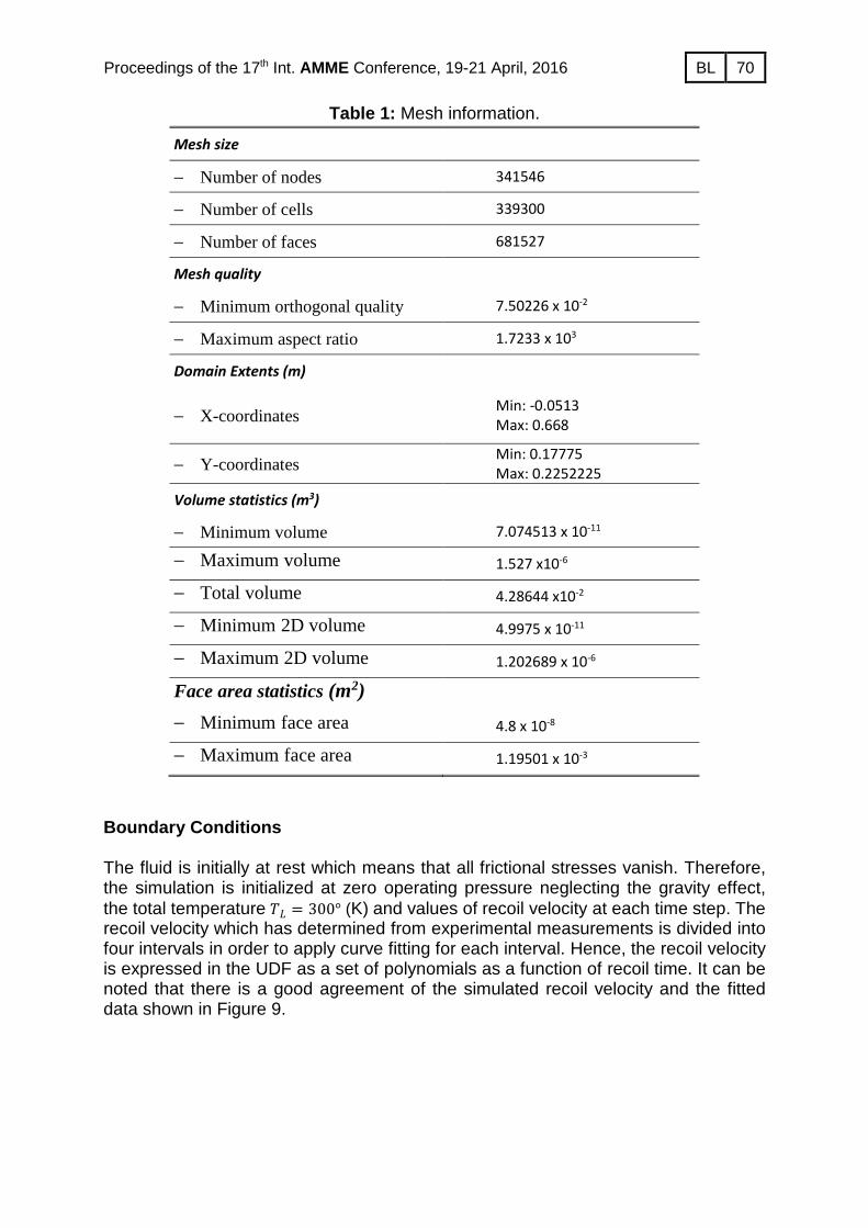
Using the values of the pressure displayed in the previous figure, the values of hydraulic resistance against recoil according to experimental work, CFD simulation and MATLAB simulation are shown in Figure 13 noting that the hydraulic resistance according to experimental work is deduced from the measured hydraulic pressure. The velocity stream traces at the plane of symmetry inside the recoil brake are shown at different time steps in Figure 14 to Figure 21. Figure 14 displays the streamlines of the liquid flow inside the recoil brake at time t=0.01s. The liquid behind the piston head flows through the clearance between its outer diameter and the inner diameter of the recoil brake cylinder. Due to the interaction of this part of the flow which leaves


Figure 13: Hydraulic resistance according to CFD model, MATLAB simulation and experimental results.

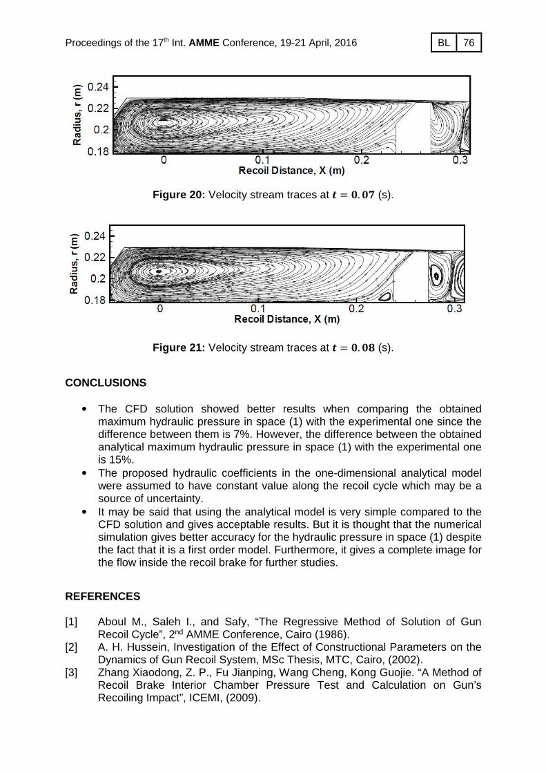
from the rear side of the piston head to its front side and the remaining liquid behind the piston head, a vortex structure is generated resulting in a saddle point SP1. Consequently, a vortex pair VP1 is formed then a vortex structure forming a saddle point SP2 followed by a vortex pair VP2 and so on. At the same time, a large primary vortex rotating in a counterclockwise direction is formed in front of the piston head. The core of this vortex is located at a distance of 22mm in front of the piston head. Figure 15 depicts the stream traces of the liquid flow inside the recoil brake at time t=0.02s. Due to the high acceleration of the piston, it can be noted that there are a lot of disturbances behind the piston head resulting in disappearing of the saddle point SP1 and changing the cores’ positions of the vortices VP1 and VP2 as well as the position of the saddle point SP2. Simultaneously, the position of the primary vortex core in front of the piston head moves towards the piston and a secondary vortex generates. It thought that the forming of the secondary vortex is due to the accelerating recoil motion of the piston head while this part of the liquid near the piston head and piston rod walls has a little energy. Figure 16 illustrates the streamlines of the liquid flow inside the recoil brake at time t=0.03s. At this time, the piston moves under a decelerating force. Therefore, the vortices behind the piston head are of less number and bigger structure. A saddle point is generated between the primary vortex in front of the piston head and a small vortex beside the wall. However there is an insignificant shift of the position of the primary vortex core and the secondary vortex is still exist. Figure 17 to Figure 21 displays the development of the flow inside the recoil brake from time t=0.04s to the end of the recoil at t=0.08s. It can be noted that the change


of the position of the primary vortex core in front of the piston head is still of insignificant value. It is thought that the insignificant change of the location of this vortex core to the end of the recoil is due to the decelerating motion which helps in decreasing the flow rate of the liquid to the front side of the piston head. The saddle point in front of the piston head disappeared as well as the secondary vortex except at the recoil end where a secondary vortex is formed. It is thought that at a specific turbulent energy value, the flow of the liquid is of sufficient energy in front of the piston head which is able to attenuate forming of other vortices. This is why the vortex structure in front of the piston head simply consists of one main vortex from time t=0.04s to the moment just before the end of the recoil.

(a)

(b) Figure 14: Velocity stream traces at � = �. � (s).

Figure 15: Velocity stream traces at � = �. �� (s).


Figure 16: Velocity stream traces at � ) �. �� (s).







CONCLUSIONS

• The CFD solution showed better results when comparing the obtained maximum hydraulic pressure in space (1) with the experimental one since the difference between them is 7%. However, the difference between the obtained analytical maximum hydraulic pressure in space (1) with the experimental one is 15%.

• The proposed hydraulic coefficients in the one-dimensional analytical model were assumed to have constant value along the recoil cycle which may be a source of uncertainty.

• It may be said that using the analytical model is very simple compared to the CFD solution and gives acceptable results. But it is thought that the numerical simulation gives better accuracy for the hydraulic pressure in space (1) despite the fact that it is a first order model. Furthermore, it gives a complete image for the flow inside the recoil brake for further studies.

REFERENCES [1] Aboul M., Saleh I., and Safy, “The Regressive Method of Solution of Gun

Recoil Cycle”, 2nd AMME Conference, Cairo (1986). [2] A. H. Hussein, Investigation of the Effect of Constructional Parameters on the

Dynamics of Gun Recoil System, MSc Thesis, MTC, Cairo, (2002). [3] Zhang Xiaodong, Z. P., Fu Jianping, Wang Cheng, Kong Guojie. “A Method of

Recoil Brake Interior Chamber Pressure Test and Calculation on Gun’s Recoiling Impact”, ICEMI, (2009).


[4] Zhang Xiaodong, Zhang Peilin, Fu Jianping, Wang Cheng. “Research on According Calculation of Hydraulic Coefficients of Recoil Brakes of Gun Based on Improved Genetic Algorithm”, International Conference on Measuring Technology and Mechatronics Automation, (2009).

[5] W.M. El-Saady, A. A. Abdallah, A.Z. Ibrahim and A. H. Hussein. “Dynamic Simulation of Tank Gun Recoil Cycle”,16th AMME Conference, Cairo (2014).

[6] Slavomir Muske, “Stability of Guns and Theory of Absorbing Gear Design”, Brno, (1968).

[7] Pijush K. Kundu and Ira M. Cohen in: “Fluid Mechanics”, 2nd edition. [8] K. J. Kang and H. I. Gimm, “Numerical and Experimental Studies on The

Dynamic Behaviors of a Gun That Uses The Soft Recoil System”, Mechanical Science and Technology, Vol. 26 , No.7, pp. 2167-2170, (2012).

[9] PENG Songjiang, ZHOU Cheng and YU Cungui, “The Numerical Simulation of Three-Dimensional Dynamic-Mesh Flow Field of a Hydraulic Buffer”, Advanced Materials Research Vol. 588-589, pp. 1264-1268, (2012).

[10] ZHANG Xiao-dong, ZHANG Pei-lin, FU Jian-ping and WANG Cheng, “Collaborative Simulation Technology Based on Matlab/Fluent”, Engineering Application Technology and Realization, Vol. 36, No. 20, pp. 220-221 (2010).

numerical simulation of flow field in coaxial gun …

Documents