Sddhan& Vol. 17, Part 2, June 1992, pp. 237-273. © Printed in India.

Numerical simulation of dispersed gas-liquid flows*

V V RANADE

Chemical Engineering Division, National Chemical Laboratory, Pune 411 008, India

MS received 27 April 1991; revised 31 October 1991

Abstract. This paper reviews the available information on numerical simulation of dispersed gas-liquid flows. Emphasis is on informing the reader about various aspects of constructing simulation models rather than giving an exhaustive literature review. The information is organised in a way so as to provide answers to the following questions: how to formulate model equations? how to select suitable algorithms and numerical techniques to solve these model equations? how to translate these into workable computer codes? how to use such codes for simulating flows in industrial equipment? Though greater emphasis is given to dispersed gas- liquid flows, the methodology can be applied to any multi-phase problem. Special features of multi-phase flow simulation over single-phase simulation are highlighted. A case of gas-liquid flow in a bubble column is presented as an illustration for the general methodology. The simulated mean flow field agrees reasonably with the experimental data. Properly validated CFD codes thus can serve as a useful tool for design engineers of multi-phase systems. Some of the common pitfalls in using simulation codes for design are also discussed. This review is expected to give an overall idea about the present state-of-art of two-phase simulation in industrial equipment.

Keywords. Gas-liquid flow; turbulence; numerical simulation.

1. Introduction

1.1 Purpose of this paper

Many energy-conversion and chemical processes involve gas-liquid two-phase flows. For example, boiling a fluid such as water or sodium and extracting heat by condensation at a different location provides a practical energy-flow process. A large number of chemical, petrochemical and biochemical processes use bubble columns as chemical reactors. Gas stirrring of liquid melts is frequently encountered in the metallurgical processing industries. In such a large class of problems, many diverse

* NCL communication no. 5172 A list of symbols appears at the end of the paper

237

238 V V Ranade

mechanisms are important in different situations. There exists a growing literature concerned with the subject, dealing with various aspects of understanding gas-liquid flows and developing suitable design methods for industrial equipment handling such flows. To list publications uncritically would do no service to the reader; and the task of sifting better from the worse is too large (and too difficult) to contemplate here.

The purpose of this review is, therefore, to acquaint the reader with some of the basic principles of detailed modelling (also called numerical simulation) as applied to gas- liquid dispersed flows. A simulation model can be used to describe the physical evolution of a complex flow system bg numerically solving the governing conservation equations for mass, momentum and energy. Such numerical simulation models can bridge the gap between theory and experiments and can therefore be applied to investigate geometric designs and/or operational changes before an expensive prototype can be built. Readily available computing resources make such an approach more attractive as compared to physical (experimental) simulation. The process of constructing a simulation model involves diverse activities from formulation of governing equations, developing modelled forms of these equations, developing various empirical submodels if necessary and developing efficient numerical techniques to solve these equations, to translating this knowledge base into computer codes to generate predictions. Excellent reviews are available on each of these activities. An important goal of this paper is to present information on all these aspects together so that the reader will be able to develop (or evaluate) a computational model with a well- understood range of validity.

1.2 Organisation of this paper

The discussion in this paper on detailed modelling of gas-liquid flows is confined to dispersed bubble flows. Section 2 attempts to identify some key characteristics of the disperesed gas-liquid flows and the modelling approaches used for such flows. It helps to define the problem we wish to solve by describing the types of time, space, physical and geometrical complexities which models must handle. Section 3 describes the development of governing equations for dispersed gas-liquid flows. The mechanism of energy transfer from the gas to the liquid phase and modelling of momentum and turbulence transport equations is described in detail.

Section 4 deals with numerical aspects for the solution of these models. Individual terms in the conservation equations and couplings between them are discussed. Most of the material on numerical aspects is discussed in finite difference language rather than finite element language. However, those conversant with both should find the translation easy. Some aspects of code development and validation are also included for the sake of completeness. Section 5 summarizes some of the recent results of detailed modelling of gas-liquid dispersed flows, which are far from comprehensive. The goal is to give the reader an idea of what kind of work has been done to date and how these models may be used. We conclude this review by some suggestions for further research on multi-phase flow simulations.

2. Dispersed gas-liquid flows: Problem characterisation

2.1 Flow characteristics

Recently many sophisticated experimental techniques have been developed for characterising multi-phase flows (Joshi et al 1990a). These newer techniques have

Numerical simulation of dispersed gas-liquid flows 2 3 9

started showing their utility, and now detailed data about turbulence in dispersed gas- liquid flows are available. It is important to note that the flow characteristics of gas- liquid flows in small diameter pipes at high throughputs (Serizawa et al 1975; Clark et al 1990; Joshi et a11990b) are very different from those in large diameter columns at smaller throughputs. The former have been dealt with by several researchers and extensive experimental data are available. These data and the proposed models (and computer codes) have been summarised by Delhaye et al (1981), while the present review deals mainly with the methods for simulating low velocity flows in large diameter columns.

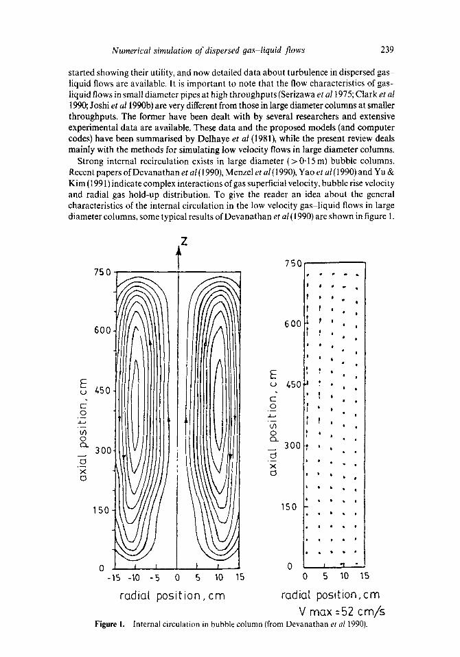
Strong internal recirculation exists in large diameter (> 0.15 m) bubble columns. Recent papers of Devanathan et al (1990), Menzel et al (1990), Yao et al (1990) and Yu & Kim (I 991) indicate complex interactions of gas superficial velocity, bubble rise velocity and radial gas hold-up distribution. To give the reader an idea about the general characteristics of the internal circulation in the low velocity gas-liquid flows in large diameter columns, some typical results of Devanathan et al (1990) are shown in figure 1.

Z

750

600

E E (-, u 450

c" o

m o o c3_

_ 3oc - ~

- ~ X

x

150

750

600 "~

450'

300

150

0 0 -is -~0 -5 0 5 10 15 0

radial posit ion, cm

Figure 1.

J II # o •

t 0 i

• I

I I

f 0 I I

I •

I I °

° I • °

° •

e

I , | o

t t I |

t , °

i

t ° • t

• I

0 • • °

° • • •

I "I •

5 10

radio[ position, cm

V max :52 cm/s Internal c irculat ion in bubble c o l u m n (from D e v a n a t h a n et a11990)•

240 V V Ranade

In addition to the internal circulation, it is worthwhile noting that experimental results show that column height does not affect centre-line velocity of the liquid in the circulation cell, provided height to diameter ratio is greater than 3. No detailed modelling efforts have been made to understand these aspects in detail. Since the characteristics of the internal recirculation and turbulence are mainly dependent on radial hold-up profile, radial phase distribution mechanism is one of the key aspects of dispersed gas-liquid flows (and as yet least understood). Almost all of the available models for the prediction of flow in the large diameter columns (Clark et al 1987, 1990; Anderson and Rice 1989; Joshi et al 1990b) require prior knowledge of the hold-up profile present in the column and are restricted to one dimension. Detailed numerical simulation models are expected to help in developing a better understanding of various aspects of gas-liquid flow in large diameter columns.

However, for the successful simulation of gas-liquid flow, model equations should represent the various time and space scales of the flow adequately. For dispersed two- phase flows, a macro time scale (tin, may be residence time in the equipment) for each phase, response time of the dispersed phase (for Stoke's regime, t* = d2po/18/~c, for larger Reynolds numbers this expression will overpredict response time), characteristic time of the energy-containing eddies of the continuous phase (re ~ k/8) and characteristic time of the dissipating eddies [th=(v/8) 1/2] are important for determining the behaviour of the system. Depending on the properties of the dispersion, the relation between t* and tc will change. Chen & Wood (1985) and Hestroni (1989) have discussed the influence of these scales on turbulence in two-phase flows in detail. Various length scales of the system also need careful consideration to achieve the desired resolution in the simulated results. It is generally assumed that the size of the dispersed phase particles is smaller than the control volumes used in the numerical scheme, which are in turn much smaller than the size of the flow system. When large scale internal flow structures are present, their scales need to be properly understood and resolved accordingly. Apart from these considerations of time and space scales, the geometric complexity of the flow system also needs to be modelled correctly. Most of the previous models use a one-dimensional framework for simulating gas-liquid flows. However, especially for flows in large diameter columns, simulations in two or even three dimensions are essential for generating reasonable predictions. This certainly makes the task of simulation difficult and computationally more expensive.

Adequate knowledge of bubble sizes and shapes, rise velocities and bubble coalescence and breakage is necessary for the realistic simulation of gas-liquid flows. The sensitivity of these micro characteristics to liquid-phase physical properties and to impurities raises further complications in the modelling of gas-liquid flows. In addition to these physical properties, the operating pressure and temperature, and mass and heat transfer from gas bubbles also affect bubble coalescence, their size and velocity distribution and therefore their flow structure. In the present paper, we attempt to develop a modular methodology of simulation, in which various submodels of coalescence etc. can be improved as our understanding of these phenomena increase. These submodels of bubble coalescence and redispersion etc. will not be discussed in this review. Moreover, though thermodynamic considerations are important for many multi-phase flows (Ahmadi & Ma 1990), in this paper we concentrate only on the mechanical aspects of tr:e flow for the sake of simplicity.

Numerical simulation of dispersed gas-liquid flows 241

2.2 Approaches for modelling of gas-liquid dispersed flows

In this section, we will consider only those models which do not require prior information about gas hold-up profile. This restriction will eliminate many previously cited one-dimensional models for g/1 flows. Zuber & Findlay (1964) have presented a derivation for the drift flux models using the concept of gas hold-up distribution parameter. This concept has been found very useful and has been used in many studies (listed by Ranade 1988). Recently, Clark et al (1990) have proposed a method for extending the one-dimensional drift flux model, eliminating the need for prior knowledge of hold-up profile. However, this method is rather ad hoc and the agreement between the predicted results and experimental data (Hills 1974) is poor. Extension of this method to the general case of gas-liquid dispersed flows is also doubtful and therefore details of it are not discussed here.

There is an interesting approach proposed by Crowe et al (1977), which has not received much attention from the modellers of gas-liquid flows. They have developed the particle-source-in-cell model for gas-droplet flows. The essential idea is to solve continuous phase transport equations in an Eulerian framework by dividing the flow field into a series of computational cells. Using this solution (which assumes that a dispersed phase is absent), dispersed phase trajectories can be calculated in a Langrangian framework. The source terms in the transport equations of the continuous phase due to the presence of the dispersed phase can then be calculated from these trajectories. The continuous phase equations are then to be solved incorporating these modified source terms. A few such iterations are sufficient to obtain the converged solution. Thus, this idea provides the simplest means to incorporate complex coupling phenomena in multi-phase flows into the calculation scheme. Dukowicz (1980) has also used a similar model for investigating liquid sprays. Though the scheme is rather empirical, the engineer or researcher can use it at least to assess the importance of bubble-liquid interactions. However, extension of this method for high throughput of gas will be difficult. Formulation of source terms due to bubbles in the transport equations of turbulence kinetic energy and rate of dissipation of turbulence energy is unclear. Therefore, this model will also not be able to predict details of the flow structure.

The third approach is to develop a detailed simulation model. A simulation model here means a complete tool for predicting the mean and turbulence characteristics of gas-liquid flows. Therefore, this will include: (a) formulation of transport equations for all the relevant physical quantities, (b) formulation of appropriate boundary conditions, (c) formulation of the necessary constitutive and closure equations, (d) algorithm for solving these equations, (e) translation of these partial differential equations into the form suitable for the numerical techniques, (f) development of computer codes for implementing the numerical solution, (g) developing validation bench marks for numerical techniques and computer codes, (h) comparison of the predicted results of the model with the experimental data to fine tune and optimise the model parameters.

Since this approach will be based on the microscopic interactions of the two phases, it is expected to mirror the actual characteristics of the flow faithfully. However, the success of this approach Will be dependent on each of the above mentioned aspects. All these aspects will be discussed in detail in the following sections.

242 V V Ranade

3. Formulation of mathematical model

3.1 Transport equations

For single-phase flows, basic transport equations are rigorously given in the form of mass, momentum and energy balances in infinitesimal volume, d V, and infinitesimal time, dr. These equations constitute the local instant field equations for density, velocity and energy, which can be applied to all the volume and time domains under consideration. However, for two-phase flows, such local instant field equations have not been attainable without adopting appropriate averaging. Several different averaging methods were used in the past. Ishii (1975) and Drew (1983) used time- averaging while Harlow & Amsden (1975), Nigmatuiin (1979), Hassanizadeh & Gray (1979), Elghobashi and Abou-Arab (1983), Rietema & Van der Akker (1983) and Ahmadi (1987) employed the volume-averaging method. Recent papers of Trapp (1986), Besnard & Harlow (1988), Kataoka & Serizawa (1989), Lahey & Drew (1989) and Ahmadi & Ma (1990) also discuss the issue of the formulation of the transport equations for two-phase flows in detail.

We will present the transport equations for two-phase dispersed flows in the general format which will be suitable for the numerical solution of the same. Each phase is treated as a continuum in any size of the domain under consideration. The phases 'share' this domain, and they may interpenetrate as they move within it. Of course, this sharing of a common location at the same time by two phases is only a convenient piece of fiction and it rests on the ideas of averaging. These ideas are easier to grasp imaginatively than to set down rigorously (although rigour can be provided if demanded, Spalding 1978). Here the reader is asked to accept that it is meaningful to conceive that (Ishii 1975, 1986; Johansen 1988):

(i) any small volume of the space in question, at any paticular time, can .be regarded as containing a volume fraction ek of the kth phase, so that if there are n phases altogether,

?1

= 1.o. (1 ) t

This means there are a sufficiently large number of dispersed phase particles in a volume characterised by the macroscopic length of the system; (ii) mass flow rate of any phase across any elementary surface within the domain at any time can be expressed in terms of the quantity ~kP~Vki, where Pk is the density of the kth phase and Vki is the local value of the velocity vector of that phase in the i direction; (iii) when the contents of finite volumes and the flow rates across finite areas are to be computed over finite intervals of time, a suitable averaging over space and time is carried out; (iv) no mass transfer occurs between two phases; (v) dispersed phase equations are restricted to one single dispersed phase particle size.

With these assumptions we can write the momentum equations in Cartesian tensor notations for each phase as:

8 ~ 0p + . = - + + +

+ Nt ,,,,tN •

Numerical simulation o f dispersed 9as-liquid f lows 243

The continuity equations can be written as:

0 ~ ( p ~ ) + ~-~x ( p ~ v~,) = o. (3)

Fk~ represents all the interphasial coupling terms except pressure. It should be noted that pressure, P, is regarded as being 'shared' by both the phases and therefore it appears in the transport equations of both the phases. The formulation of the pressure term has occasioned some uncertainty among the writers on the subject (Spalding 1978); and it is sometimes thought that different pressures 'ought' to be provided for each phase. The pressure inside the individual gas bubble is related to the pressure of the continuous phase via surface tension and the bubble radius. However, this pressure inside the bubble has no relation to the flow of the dispersed phase and therefore is irrelevant for the description of flow equations (Rietema and Van den Akker 1983). Pressure at the interface of gas and liquid phases can be assumed to be equal to the liquid phase pressure since equations are spatially averaged over a volume larger than the bubble (Johansen 1988). Thus, for most of the practical circumstances (especially in chemical reactors), where the speed of sound in each phase is large compared to the velocities of interest, the assumption of microscopic pressure equilibration is adequate (Spalding 1978; Drew 1983).

The restriction of one single particle size can be removed by providing one set of continuity and momentum equations for each particle size fraction. If a particle size distribution is represented by M size classes, there will be 4M equations to describe only the dispersed phase. If mass transfer and/or reaction is taking place between the phases, source terms accounting these phenomena need to be included into the mass conservation equations (for example, Boyson et al 1982).

Interphasial coupling terms make two-phase flows fundamentally different from single-phase flows. The formulation of Fk~, therefore, must proceed carefully, with attention being paid to the force balance for single particles and to any possible inconsistencies. The interphase coupling terms must satisfy the following relation:

E l i = - - F21, (4)

where subscripts 1 and 2 denote gas (dispersed) and liquid phase respectively. For dispersed two-phase flows, there are at least two transient forces acting at the

interface in addition to the standard drag force, namely virtual mass force arising from the inertia effect (Ishii & Zuber 1979; Auton 1981; Cook & Harlow 1986) and the Basset force due to the development of a boundary layer around a bubble (Basset 1888). In addition to this, the transversal lift force on the bubble is created by gradients in relative velocity across the bubble diameter (Thomas et al 1983, pp. 169-184). The interphase momentum transport term for gas phase (subscript 1) can therefore be written as:

FI~ = (3/4)~1 e2P2CoB( V2i - Vu)] Vzi- Vul/dn +

+ ea ~2pz fv(DV2i /Dt - DV1JDt ) +

;o + eae2fn(61~/dn) {(DV2i/Dt - DVll/Dt)/Ev(t - t ' )] l /Z}dt ' +

+ ele2P2fLem, e,a( V2,, - Vl , , )OV2Jtxr , (5)

where e,a is the Levi-Cevita tensor. The transversal lift coefficient, fL, is 0-5 for potential flow and spherical particles (Drew et al 1979). For very low bubble Reynolds

244 V V Ranade

number (<< 1), the Basset force coefficient, fn, is calculated to be 1.5. The virtual mass terms used by Drew et al (1979) and Cook & Harlow (1986) contain additional terms consisting of the gradients of slip velocity. The virtual mass coefficient, fv , is 0"5 for rigid, spherical solid particles (Maxey & Riley 1983). This value is generally shape dependent, for example, Cook & Harlow (1986) used fv = 0.25 for bubbles in water. CoB is a drag coefficient which is a function of bubble Reynolds number. Morsi & Alexander (1972) have reported empirical correlations of drag coefficient-Reynolds number data for solid particles for a very wide range of Reynolds numbers. However, the drag function of bubbles is more complicated than that of solid particles due to their deformability. Depending on the Reynolds number (these dimensionless numbers are defined using liquid phase physical properties, the subscripts are not shown for simplicity), Eotvos number (Eo = gApd2n/a), Morton number (M = gla4Ap/p2a 3) and Weber number (We = pV2da/a), there are different regimes of drag function (Clift et al 1978). For the commonly encountered range of bubble Reynolds numbers, that is 500 < ReB < 5000, the following correlation can be used to estimate drag coefficient (Clift et al 1978):

Co8 = 0-622/(0-235 + (1/Eo)). (6)

For the case of flow of a swarm of bubbles, it is necessary to modify the above expression to account for the fact that a group of rising bubbles tend to follow one another's wakes. Measurements of Tsuji et al (1984) for two spheres in the Reynolds number range of 100 to 200 can be expressed as:

CoB = Co0(1 - [dB/LB]2), (7)

where Coo is the drag coefficient for a single isolated bubble and LB is the distance between the centres of two spheres, which can be easily related to the fractional gas hold-up in a given control volume.

The two-phase momentum equations must, if they are consistent, reduce to single-phase Navier-Stokes equations if there is no interphasial slip or if dispersed phase hold-up is zero. If the no interphasial slip condition (in other words, drag coeffÉcient equal to infinity) is inserted in the momentum equations (2), we get the Navier-Stokes equation in terms of mixture density (Zekp k) and mixture viscosity (Xek/ak). This equation will cause gravitationally driven currents if there are gradients in mixture density. However, it can be shown that the gradients of phase hold-up will not be able to create gravitationally driven currents in the absence of interphasial drag (Johansen 1988).

The discussion of the turbulence in dispersed two-phase flows was excluded till now. However, it is necessary to understand the mechanism of the generation of turbulence by gas bubbles and to develop corresponding phenomenological models for simulating the energy exchange between gas and liquid phases. These aspects will be discussed below before we present the modelled form of the transport equations in § 3-3.

3.2 Turbulene in gas-liquid flows

When a gas bubble travels through a body of liquid from a location with higher hydrostatic pressure to that with a lower hydrostatic pressure, it dissipates its energy. Part of this released energy gets dissipated at the gas-liquid interface and in the wake

Numerical simulation of dispersed gas-liquid flows 245

behind the bubble. The remainder gets dissipated in the bulk liquid phase, generating corresponding additional turbulence. For lower superficial gas velocities, most of the energy gets dissipated in the localised region around bubbles. Therefore, the scale of the generated turbulence is of the order of the bubble diameter. Joshi (1983) has proposed a model based on overall energy balance to estimate turbulence intensity for such a case. For higher superficial gas velocities, however, a significant part of the energy released by the gas gets dissipated in the bulk of liquid, which leads to generation of large scale structures in the gas-liquid flows. Modelling of this additional turbulence is a real challenge for the successful simulation of gas-liquid flows.

For the closure of momentum equations, concept of eddy viscosity is generally employed. Deb Roy et al (1978), Melville & Bray (1979), Sato et al (1981), Sahai & Guthrie (1982), Salcudean et al (1985) and Clark et al (1987) have proposed some empirical formulae for estimating effective turbulent viscosity in two-phase flows. However these equations prescribe a unique value of turbulent viscosity for the entire flow field and therefore fail to simulate effects of its variation within the system. To account for this variation, the desired turbulence model should be able to predict the turbulence length and velocity scales correctly. Two-equation turbulence models are the simplest models that promise success for flows in which the length scale cannot be prescribed empirically. Among the various two-equation models, the k - 8 model is most widely tested and will be adopted here as a basic framework for the simulation of two-phase turbulent flows. The following subsection describes the modelled forms of the turbulent momentum transport equations.

3.3 Turbulence modelling of two-phase flow equations

Let us consider the stationary mass and momentum conservation equations. The instantaneous quantities ~b in all the equations are now replaced by ~b + ~b', where the first quantity represents the time average of q~ and the latter q~' represents the instantaneous variations of ~b around its mean value. This amounts to introducing Reynolds averaging procedure. The time-averaged (denoted by brackets ( ) ) mass conservation equation is then:

Pk (~t (~k)+ ~---~ (~k Vk, + (~kV~,))) -----0. (8)

The first term represents the convective mass transport and the second term expresses the turbulent diffusive mass transport. The time-averaged momentum equation can be written as:

p~ ~ ( ~ ~ + ( ~ v ~ ) ) + (~ v~j v~) = - ~ - ~ +

-p~-~xj(~(v~jv~) + V~(vk~k) + ~ (v~ ,~ ) + (~kv~jv~) ) ×

× pkgkOi + (Fk i ) + (viscous shear terms). (9)

These time-averaged transport equations demonstrate the effects of turbulence via various higher order and unknown terms. The viscous shear terms normally can be neglected in comparison with the turbulent shear terms.

246 V V Ranade

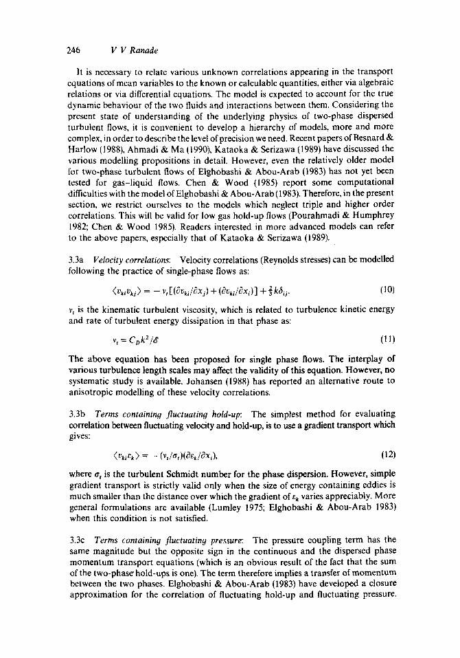
It is necessary to relate various unknown correlations appearing in the transport equations of mean variables to the known or calculable quantities, either via algebraic relations or via differential equations. The model is expected to account for the true dynamic behaviour of the two fluids and interactions between them. Considering the present state of understanding of the underlying physics of two-phase dispersed turbulent flows, it is convenient to develop a hierarchy of models, more and more complex, in order to describe the level of precision we need. Recent papers of Besnard & Harlow (1988), Abmadi & Ma (1990), Kataoka & Serizawa (1989) have discussed the various modelling propositions in detail. However, even the relatively older model for two-phase turbulent flows of Elghobashi & Abou-Arab (1983) has not yet been tested for gas-liquid flows. Chen & Wood (1985) report some computational difficulties with the model of Elgbobashi & Abou-Arab (1983). Therefore, in the present section, we restrict ourselves to the models which neglect triple and higher order correlations. This will be valid for low gas hold-up flows (Pourahmadi & Humphrey 1982; Chen & Wood 1985). Readers interested in more advanced models can refer to the above papers, especially that of Kataoka & Serizawa (1989).

3.3a Velocity correlations: Velocity correlations (Reynolds stresses) can be modelled following the practice of single-phase flows as:

( Vkl Vk. i ) = -- V, [ (OVkl/t~X i ) + (OVkl/OXi ) ] + 2 k60. (10)

v, is the kinematic turbulent viscosity, which is related to turbulence kinetic energy and rate of turbulent energy dissipation in that phase as:

v t = C D k 2 / ~ (11)

The above equation has been proposed for single phase flows. The interplay of various turbulence length scales may affect the validity of this equation. However, no systematic study is available. Johansen (1988) has reported an alternative route to anisotropic modelling of these velocity correlations.

3.3b Terms containing f luc tuat ing hold-up: The simplest method for evaluating correlation between fluctuating velocity and hold-up, is to use a gradient transport which gives:

(12)

where tr t is the turbulent Schmidt number for the phase dispersion. However, simple gradient transport is strictly valid only when the size of energy containing eddies is much smaller than the distance over which the gradient of ~k varies appreciably. More general formulations are available (Lumley 1975; Elghobashi & Abou-Arab 1983) when this condition is not satisfied.

3.3c Terms containing f luc tuat ing pressure: The pressure coupling term has the same magnitude but the opposite sign in the continuous and the dispersed phase momentum transport equations (which is an obvious result of the fact that the sum of the two-phase hold-ups is one). The term therefore implies a transfer of momentum between the two phases. Elghobashi & Abou-Arab (1983) have developed a closure approximation for the correlation of fluctuating hold-up and fluctuating pressure.

Numerical simulation of dispersed oas-liquid flows 247

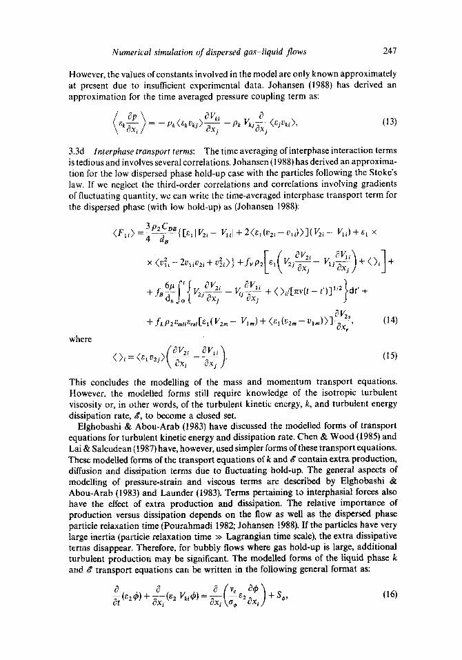
However, the values of constants involved in the model are only known approximately at present due to insufficient experimental data. Johansen (1988) has derived an approximation for the time averaged pressure coupling term as:

Opt OV.i c~ ~k ~ = - Pk (ek Vkj) ~ - Pk Vkj ~jXj (eivk`)' (13)

3.3d lnterphase transport terms: The time averaging ofinterphase interaction terms is tedious and involves several correlations. Johansen (1988) has derived an approxima- tion for the low dispersed phase hold-up case with the particles following the Stoke's law. If we neglect the third-order correlations and correlations involving gradients of fluctuating quantity, we can write the time-averaged interphase transport term for the dispersed phase (with low hold-up) as (Johansen 1988):

where

3 Pz CoB ( F l i ) - 4 dn {[ellV2i- l /]i l+2@l(vzl-vii))](V2i- Vll)--~-e 1 X

X (v2i--2v,iv2i+vZi)}+fvp2[ei{V , \ 2j~x i - ,V2i V,,-~x~)+c~V'i'~ ( ) , ] +

+j~6/~ f J'V..¢71 2/ _ E, c~Vll db jo ~ 2J OXj i3 OX j + ( )i/[r~v(t - t')-] 1/2. dr '+

+ fLP2~m,~,st[el( Vzr . -- Vim ) + (~!(Vz,. - vl,.))] ~Vx2:, (14)

(15)

This concludes the modelling of the mass and momentum transport equations. However, the modelled forms still require knowledge of the isotropic turbulent viscosity or, in other words, of the turbulent kinetic energy, k, and turbulent energy dissipation rate, g, to become a closed set.

Elghobashi & Abou-Arab (1983) have discussed the modelled forms of transport equations for turbulent kinetic energy and dissipation rate. Chen& Wood (1985) and Lai & Salcudean (1987) have, however, used simpler forms of these transport equations. These modelled forms of the transport equations of k and g contain extra production, diffusion and dissipation terms due to fluctuating hold-up. The general aspects of modelling of pressure-strain and viscous terms are described by Elghobashi & Abou-Arab (1983) and Launder (1983). Terms pertaining to interphasial forces also have the effect of extra production and dissipation. The relative importance of production versus dissipation depends on the flow as well as the dispersed phase particle relaxation time (Pourahmadi 1982; Johansen 1988). If the particles have very large inertia (particle relaxation time >> Lagrangian time scale), the extra dissipative terms disappear. Therefore, for bubbly flows where gas hold-up is large, additional turbulent production may be significant. "['he modelled forms of the liquid phase k and g transport equations can be written in the following general format as:

(16)

248 V V Ranade

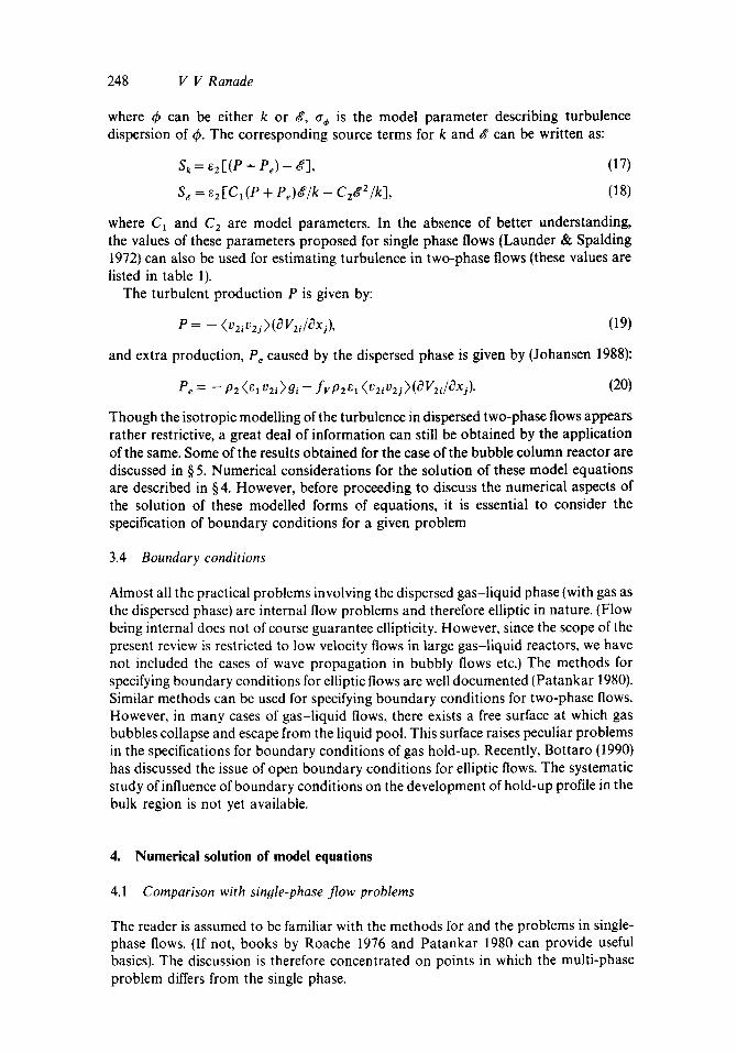
where ~b can be either k or ~, ~r~ is the model parameter describing turbulence dispersion of ~b. The corresponding source terms for k and ~ can be written as:

Sk = ezl(P + P c ) - ~], (17)

S~. = •2 [ ' C I ( P + Pe)g/k - C 2 g 2 / k ] , (18)

where C1 and C2 are model parameters. In the absence of better understanding, the values of these parameters proposed for single phase flows (Launder & Spalding 1972) can also be used for estimating turbulence in two-phase flows (these values are listed in table 1).

The turbulent production P is given by:

p = - ( 1 ) 2 i v 2 j ) ( O V 2 i / ~ x j ) , (19)

and extra production, Pe caused by the dispersed phase is given by (Johansen 1988):

Pe = -- P2 (el v2i )Oi -- fvP2el (v21v2.i)(OV21/Oxj)" (20)

Though the isotropic modelling of the turbulence in dispersed two-phase flows appears rather restrictive, a great deal of information can still be obtained by the application of the same. Some of the results obtained for the case of the bubble column reactor are discussed in § 5. Numerical considerations for the solution of these model equations are described in § 4. However, before proceeding to discuss the numerical aspects of the solution of these modelled forms of equations, it is essential to consider the specification of boundary conditions for a given problem

3.4 Boundary conditions

Almost all the practical problems involving the dispersed gas-liquid phase (with gas as the dispersed phase) are internal flow problems and therefore elliptic in nature. (Flow being internal does not of course guarantee ellipticity. However, since the scope of the present review is restricted to low velocity flows in large gas-liquid reactors, we have not included the cases of wave propagation in bubbly flows etc.) The methods for specifying boundary conditions for elliptic flows are well documented (Patankar 1980). Similar methods can be used for specifying boundary conditions for two-phase flows. However, in many cases of gas-liquid flows, there exists a free surface at which gas bubbles collapse and escape from the liquid pool. This surface raises peculiar problems in the specifications for boundary conditions of gas hold-up. Recently, Bottaro (1990) has discussed the issue of open boundary conditions for elliptic flows. The systematic study of influence of boundary conditions on the development of hold-up profile in the bulk region is not yet available.

4. Numerical solution of model equations

4.1 Comparison with single-phase flow problems

The reader is assumed to be familiar with the methods for and the problems in single- phase flows. (If not, books by Roache 1976 and Patankar 1980 can provide useful basics). The discussion is therefore concentrated on points in which the multi-phase problem differs from the single phase.

Numerical simulation of dispersed 9as-liquid flows 249

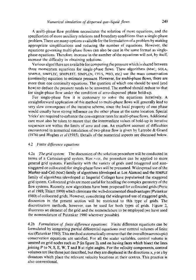
A multi-phase flow problem necessitates the solution of more equations, and the specification of more auxiliary relations and boundary conditions than a single-phase problem. There are many options available for the formulation of a problem by making appropriate simplifications and reducing the number of equations. However, the equations governing multi-phase flows can also be cast in the same format as single- phase equations. Therefore, increase in the number of the equations will not, by itself, increase the difficulty in obtaining solutions.

Various algorithms are available for computing the pressure which is shared between three momentum equations for single-phase flows. These algorithms (MAC, SOLA, SIMPLE, SIMPLEC, SIMPLEST, SIMPLEN, CELS, PISO, etc.) use the mass conservation (continuity) equation to estimate pressure. However, for multi-phase flows, there are more than one continuity equations. The question of which one should be used (and how) to deduce the pressure needs to be answered. The method should reduce to that for single-phase flow under the condition of zero-dispersed phase hold-up.

For single-phase flow it is customary to solve the equations iteratively. A straightforward application of this method to multi-phase flows will generally lead to very slow convergence of the iterative scheme, since the local property of one phase would usually have strong influence on the other phase at the same location. Special 'tricks' are required to enhance the convergence rates for multi-phase flows. Additional care must also be taken to ensure that the intermediate values of hold-up in iterative sequences are within the limits of zero and one. An excellent account of difficulties encountered in numerical simulation of two-phase flow is given by Latrobe & Grand (1976) and Hughes et al (1985). Details of the numerical aspects are discussed below.

4.2 Finite difference equations

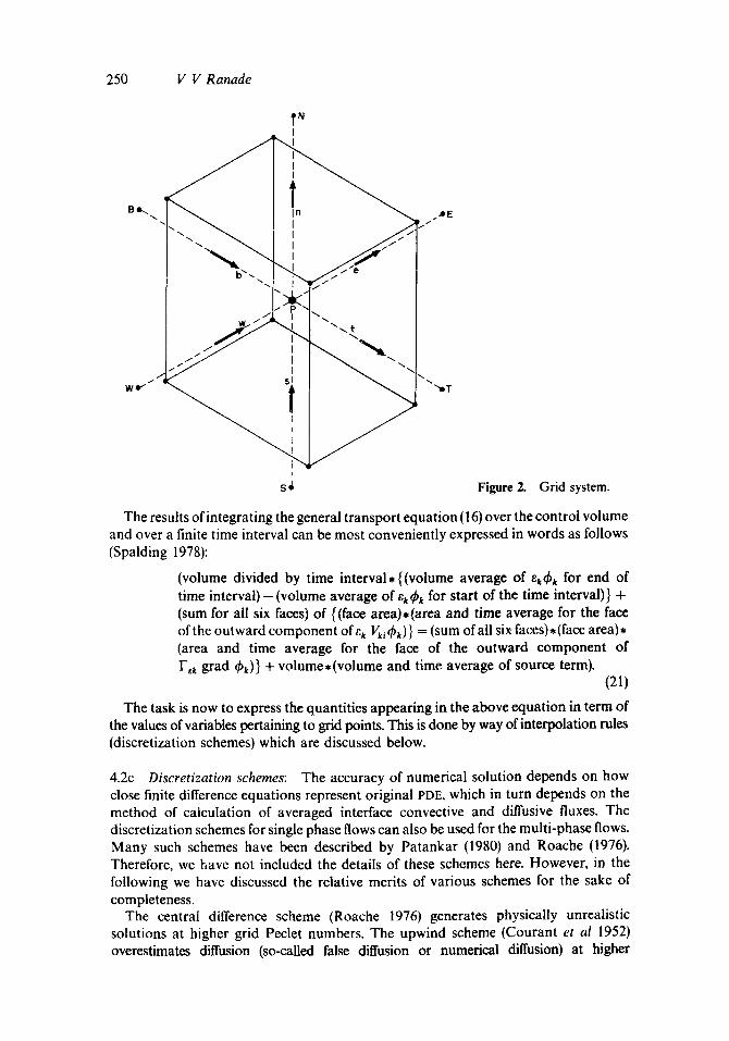
4.2a The 9rid system: The discussion of the solution procedure will be conducted in terms of a Cartesian-grid system. Hov acer, the procedure can be applied to more general grid systems. Familiarity with the variety of grids used (staggered and non- staggered or collocated) for single-phase flows will be presumed. Widespread use of the Marker-and-Cell (MAC) family of algorithms (developed at Los Alamos) and the SIMPLE family of algorithms (developed at Imperial College) have popularised the staggered grid system. Collocated grids are more useful for handling the complex geometry of the flow systems. Recently, new algorithms have been proposed for collocated grids (Peric et a11988; Thiart 1990) which eliminate the well-documented disadvantages (Patankar 1980) of collocated grids. However, considering thg widespread use of staggered grids, discussion in the present section will be restricted to this type of grids. The discretization methods, however, can be used for both types of grids. Figure 2, illustrates an element of the grid and the nomenclature to be employed (we have used the nomenclature of Patankar 1980 wherever possible).

4.2b Formulation of finite difference equations: Finite difference equations can be formulated by integrating partial differential equations over control volumes of finite size (P.atankar 1980). This method automatically ensures that the overall (macroscopic) conservation equations are satisfied. For all the scalar variables, control volume is centred on grid nodes such as P (in figure 2), and on having faces which bisect the lines joining P to N, S, E, W, T and B at right angles. For the velocity components, control volumes are like those just described, but they are displaced in the directions x, y or z by distances which place the relevant velocity locations at their centres. This practice is also conventional.

250 V V Ranade

I

Bo~\ I~~ ~E ... I

\ I "~..

We" ~ ~Y

s~ Figure 2. Grid system.

The results of integrating the general transport equation (l 6) over the control volume and over a finite time interval can be most conveniently expressed in words as follows (Spalding 1978):

(volume divided by time interval,{(volume average of e, kf~k for end of time interval)- (volume average of ekqbk for start of the time interval)} + (sum for all six faces) of {(face area).(area and time average for the face of the outward component of ek Vki Ok)} = (sum of all six faces), (face area), (area and time average for the face of the outward component of F~k grad thk)} + volume.(volume and time average of source term).

(21)

The task is now to express the quantities appearing in the above equation in term of the values of variables pertaining to grid points. This is done by way of interpolation rules (discretization schemes) which are discussed below.

4.2c Discretization schemes: The accuracy of numerical solution depends on how close finite difference equations represent original PDE, which in turn depends on the method of calculation of averaged interface convective and diffusive fluxes. The discretization schemes for single phase flows can also be used for the multi-phase flows. Many such schemes have been described by Patankar (1980) and Roache (1976). Therefore, we have not included the details of these schemes here. However, in the following we have discussed the relative merits of various schemes for the sake of completeness.

The central difference scheme (Roache 1976) generates physically unrealistic solutions at higher grid Peclet numbers. The upwind scheme (Courant et al 1952) overestimates diffusion (so-called false diffusion or numerical diffusion) at higher

Numerical simulation of dispersed 9as-liquid flows 251

Peclet numbers, while for smaller grid Peclet numbers, it is not as accurate as the central difference scheme. These considerations led Spalding (1972) to develop the exponential differencing (ED) scheme. This scheme is based on exact solution of the steady, one- dimensional convective-diffusion equation without any source term. This scheme is more accurate than the upwind scheme. Since exponentials are expensive to compute, several approximations of ED such as hybrid scheme (Spalding 1972), power law schemes (Patankar 1980; Amano 1984) have been proposed. The assumption of local one-dimensional transport of these schemes lead to errors when multi-dimensional problems are being solved. These errors, which manifest in the form of false diffusion normal to flow direction, become important when there is a large angle between the flow and grid lines. Raithby (1976) has proposed the skewed upwind differencing (SUWD) scheme to minimise this false diffusion. Though, the SUWD scheme reduces skewness errors, it is also (like the conventional upwind scheme) only first order accurate, and it fails to give accurate solutions in the presence of source terms.

Leonard (1979) has proposed quadratic upwind interpolation (QUICK) for the estimation of face fluxes. QUICK has shown to be more accurate than ED (Leschziner 1980) in many cases+ however, unlike ED it is not unconditionally stable (Han et al 1981). Wong & Raithby (1979) have proposed a locally analytic differencing (LOAD) scheme, which places the source term in its dominating position while computing interface fluxes. This scheme retains its second-order accuracy at high grid Peclet numbers (Prakash 1984). However, it requires iterative procedure to compute interface fluxes and is rather expensive to implement. ALias et al (1977) have used a second-order upwind differencing scheme. Shyy (1985) has shown that second-order upwind scheme is better than the QUICK scheme. Huh et al (1986) have proposed a method for reducing numerical diffusion in the upwind scheme. Runchal (1986) has also proposed a modified central difference scheme with unconditional stability (called CONDlr). Braga (1990) has proposed a new higher order five-point scheme. Many studies comparing the properties of various differencing schemes are available (Peric et al 1988; Braga 1990; Zurigat & Ghajar 1990). The desire to use higher order approximations (and small grid sizes) to ensure accuracy must be balanced against limitations imposed by the complexity of the problem being solved, the availability of the computing equipment and stability of the solution algorithm. Among the various schemes, QUICK and second-order upwind differencing schemes look more attractive from the point of view of accuracy and ease of implementation. However, both these methods may generate unphysical over- or undershoots. For a beginner to two-phase flow computations, it might be advisable to start with some power law variation of the ED scheme till he/she understands the characteristics of the problem at hand.

4.2d Discretized equations

Discretization schemes described in the references cited above, can be used to translate the verbal equation (21) in terms of node variables. The source terms of each equation are also integrated over the control volume and linearized following the methods discussed by Patankar (1980). All these procedures are the same as those for single-phase flows. The only features specific to two-phase flows are the fractional hold-ups, E~ and the interaction parts of the source terms. Whenever, ek is included in the diffusive transport, the harmonic mean should be used to compute ek at the interface. Application of these rules results in a discretized form of the PDE at any grid node, which can be usefully expressed in the form (reference to phase k has been

252 V V Ranade

omitted for the sake of clarity):

q~v = aNckN + as~b~ + aE~E + ave + ~ve + ar~br + a~dPn + apoqbt, + sC~ (22) bN + bs + bE + bye + b r + bnbeo - SP,

The coefficient a's consist of an inflow convection contribution and a diffusion contribution, whereas the b's consist of an outflow contribution and a diffusion contribution. The exact expressions for a's and b's will depend on the discretization scheme used. To facilitate understanding, the expressions for a's and b's derived using the upwind scheme are given below:

a n = A.([0, - ~. V.] + ( F . e . / ( y N - YP))), (23)

b N = A.([0, e. V.] + (F.e./(y N - yp))), (24)

where [] indicates maximum value. A. is cell area of north face, (Yu - Ye) is internode distance and Fe. is the harmonic mean of the products of F and e at nodes P and N. The expression for aeo and beo can be conveniently written as:

apo = ~p( V . . / A t ) , (25)

beo = ~e( Vce,/At ). (26)

Equation (22) contains source terms in the denominator as well as in the numerator of the RHS. This is based on a source term linearization practice as (Patankar 1980):

s0 = + (27)

This form anticipates, to some extent, the change which occurs in the value of the source term after the completion of the current iteration. For linearizing the source terms, it is useful to recognise that the source term often also constitutes terms having significances similar to the a's and b's

It is worth noting that the mass conservation equation implies the following relationship between the a's and b's:

au - bN + as - bs + a t - b~ + ave - bw + ar - br +

+ an - bB + aeo -- bvo = 0, (28)

when there is no mass exchange between the phases. The equation for fractional hold-up, ~, has a similar form of the equation for 4~k,

(22). However, the a's and b's must be defined without the ek's. As a consequence of this, the a's and b's for the ek equation are not related as in the case of 4~,. Thus during the approach to the converged solution, the a's and b's may not be in proper balance; therefore non-physical values of ek can be generated. This necessitates the special overwriting procedures for ek in two-phase computations.

The equation for velocity components also have a form similar to (22). Particular interest attaches to the role of pressure, which appears in the source term. It is also worth noting that the discretized equation for the velocity of one phase will involve the velocities of other phases at the same node. The interaction coefficients between velocities of different phases at the same node will dictate the progress towards convergence.

The discretized equations of the pressure and pressure corrections will be discussed in the next subsection.

Numerical simulation of dispersed gas-liquid flows 253

4.3 Algorithms

4.3a For treating velocity-pressure coupling: Many algorithms like SIMPLE and SIMPLER (Patankar 1980), SIMPLEST (Spalding 1980), SlMPLEC (Van Doormal & Raithby 1984), CELS (Galpin et al 1985), PSIO (Issa 1986) have been proposed for solving pressure-velocity coupling for single-phase flows. One can in principle use similar concepts to derive the pressure correction equation for two-phase flows. The equation for pressure can also be derived using procedures of single-phase flow. For the pressure correction equation, however, a decision has to be made about which continuity equation to be used for the derivation. Spalding (1978) has proposed the use of an overall continuity equation (that is the sum of continuity equations of all phases) for deriving pressure corrections in his IPSA algorithm. Fletcher & Thyagraja (1989) and Bush & Marshall (1989) have also used overall continuity equations for estimating pressure corrections.

Thus, the pressure correction equation can be obtained by using differential coefficients of velocity with pressure (Spalding 1978). These coefficients can easily be computed by casting the discretized equations of velocity in the following form:

= ( Vke "1- g~e(Pp - - P E ) ) / h * , Vk~ * (29)

wherein the expressions for V*~, g*e and h~' are obtained from the discretization scheme. Differentiation of this equation with Pp and PE yield:

O Vk~/OP e = - O Vke/OP E = 9k~/hk. (30)

These coefficients along with similar ones for the remaining five velocities will be used for developing the pressure correction equation.

The overall continuity equation in algebraic form can be written as:

n

~ (flke Vk~ + flkw Vkw + ..-) = 0. (31) 1

Here, the definitions of coefficients can be deduced from the summation of individual continuity equations and the interpolation rules. The velocity field generated based on correct pressure field will not satisfy the overall continuity equation and there will be net accumulation or loss from each cell, say ER. To find the pressure corrections (following the methods of single-phase flows), it is now supposed that all the pressures in the field are modified to change the velocities and to eliminate the errors in the continuity equation. Differentiation of the overall continuity equation therefore leads to."

, t~V~e , + (32)

This is the required equation for pressure correction at the grid point P, P~, in terms of six 9ressure corrections of the neighbouring points and differential coefficient of velocity. It is not vital that velocity differential coefficients should be precise, however, they must have the right sign. Once the pressure correction field is obtained by solving (32), velocity corrections can be computed and added to the in-store values. This will result in a velocity field which will satisfy the overall continuity equation at every grid point.

254 V V Ranade

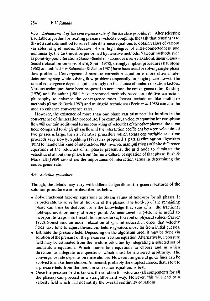
4.3b Enhancement of the converyence rate of the iterative procedure: After selecting a suitable algorthm for treating pressure-velocity coupling, the task that remains is to devise a suitable method to solve finite difference equations to obtain values of various variables at grid nodes. Because of the high degree of inter-connectedness and nonlinearity, the task must be performed by iterative methods. Various methods such as point-by-point iteration (Gauss-Seidel or successive over-relaxation), linear Gauss- Seidel (relaxation versions of ADI, Smith 1978), strongly implicit procedure (siP, Stone 1968) or modified siP (Schneider & Zedan 1981) have been used for solving single-phase flow problems. Convergence of pressure correction equation is more often a rate- determining step while solving flow problems (especially for single-phase flows). The rate of convergence depends quite strongly on the choice of under-relaxation factors. Various techniques have been proposed to accelerate the convergence rates. Raithby (1976) and Patankar (1981) have proposed methods based on additive correction philosophy to enhance the convergence rates. Recent techniques like multistep methods (Oran & Boris 1987) and multigrid techniques (Peric et al 1988) can also be used to enhance convergence rates.

However, the existence of more than one phase can raise peculiar hurdles in the convergence of the iteration procedure. For example, a velocity equation for two-phase flow will contain additional terms consisting of velocities of the other phase at the same node compared to single-phase flow. If the interaction coefficient between velocities of two phases is large, then an iterative procedure which treats one variable at a time proceeds very slowly. Spalding (1978) has proposed a partial elimination algorithm (PEA) to handle this kind of interaction. PEA involves manipulations of finite difference equations of the velocities of all phases present at the grid node to eliminate the velocities of all but one-phase from the finite difference equation of that phase. Bush & Marshall (1989) also stress the importance of interaction terms in determining the convergence rate.

4.4 Solution procedure

Though, the details may vary with different algorithms, the general features of the solution procedure can be described as below.

• Solve fractional hold-up equations to obtain values of hold-ups for all phases. It is preferable to solve for all but one of the phases. The hold-up of the remaining phase can then be deduced from the knowledge that sum of all the fractional hold-ups must be unity at every point. As mentioned in §4.2d it is useful to incorporate 'traps' into the solution procedure ek to avoid unphysical values (Carver 1982). Sometimes, an under-relaxation of ek is introduced, in order that velocity fields have time to adjust themselves, before ek values move far from initial guesses.

• Estimate the pressure field. Depending on the algorithm used, it may be done via solution of the pressure or the pressure correction equation. Alternatively, a pressure field may be estimated from the in-store velocities by integrating a selected set of momentum equations. Which momentum equations to choose and in which direction to integrate are questions which must be answered arbitrarily. The convergence rate depends on these choices. However, no general guide lines can be evolved to make these choices. At present, probably the simplest choice, that is to use a pressure field from the pressure correction equation, is best.

• Once the pressure field is known, the solution for velocities (all components for all the phases) can proceed in a straightforward way. However, this will lead to a velocity field which will not satisfy the overall continuity equations.

Numerical simulation of dispersed gas-liquid flows 255

• To eliminate the error from the continuity equation, pressure and velocity need to be modified. The pressure correction field needs to be solved using the coefficients generated from the recently obtained velocity fields. Velocity corrections can then be calculated from the pressure correction field. The modified velocity field using these velocity corrections then satisfies overall continuity at every point.

• This cycle of adjustments is performed many times, until the errors remaining in all the equations are acceptably small It is hoped that at each repetition of the cycle, errors in the equations become smaller and smaller. When this hope is not realised, the failure is generally attributable to the unusual geometrical proportions of the cell, to inadequate under-relaxation or to some non-standard coupling between equations which requires an amendment to the solution procedure. However, in most of the cases, this general procedure has been shown to be satisfactory.

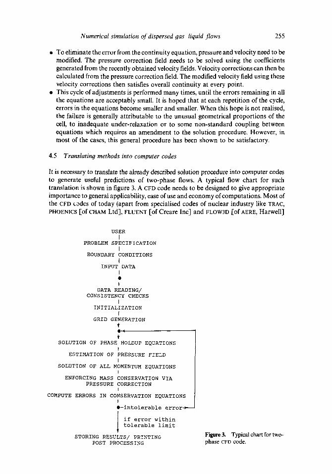
4.5 Translating methods into computer codes

It is necessary to translate the already described solution procedure into computer codes to generate useful predictions of two-phase flows. A typical flow chart for such translation is shown in figure 3. A CFD code needs to be designed to give appropriate importance to general applicability, ease of use and economy of computations. Most of the CFD codes of today (apart from specialised codes of nuclear industry like TRAC, PHOENICS [of CHAM Ltd], FLUENT [of Creare Inc] and FLOW3D [of AERE, Harwell]

USER I

PROBLEM SPECIFICATION I

BOUNDARY CONDITIONS I

INPUT DATA I

I DATA READING/

CONSISTENCY CHECKS I

INITIALIZATION [

GRID GENERATION t 04

SOLUTION OF PHASE HOLDUP EQUATIONS I

ESTIMATION OF PRESSURE FIELD I

SOLUTION OF ALL MOMENTUM EQUATIONS I

ENFORCING MASS CONSERVATION VIA PRESSURE CORRECTION

I COMPUTE ERRORS IN CONSERVATION EQUATIONS

i

• -intolerable error~---

I if error within tolerable limit

STORING RESULTS/ PRINTING POST PROCESSING

Figure 3. Typical chart for two- phase CFD code.

256 V V Ranade

are the best-known codes for the simulation of three-dimensional, multiphase flows) derived from the code TEACH from Imperial College (Gosman & Pun 1974) or from the MAC code from Los Alamos (Harlow & Welch 1965). It is necessary to identify the numerical tasks which take the major share ofcPu time so that special measures can be taken to optimise that part of the code. Recently, Cross et al (1989) have discussed the trends in CFD software engineering which are useful for the new code developer.

Since the numerical simulation approach is fast becoming popular with designers of multi-phase systems, it is necessary to caution them against the trust placed on predictions of codes which are not properly validated. CFD generated predictions of multi-phase flows can go wrong for two main reasons (other than human error and machine malfunction): they may be based upon physically incorrect mathematical representations of basic physical phenomena or upon numerically deficient representation (incorrect discretization, crude grids or incomplete convergence). Inadequacies of the first kind are almost always present because the physics of multi-phase flows is not yet properly understood. However, it is the responsibility of the CFD analyst to eliminate or minimise the inadequacies in the numerical representation. The bounds of the numerical accuracy of the specific code can be obtained by comparing results with the analytical solution of some simple but representative problem. Villasenor & Spalding (1987) have presented the fourteen problems which can be used for the benchmarking exercise. Spalding (1989) has presented the detailed results for the case of a ID, monopropellant rocket problem for the purpose of numerical benchmarking of the multi-phase flow simulation codes.

5. Simulation of gas-liquid flows

5.1 Methodology

Before embarking on an exercise of simulating any flow system, it is essential to understand and quantify various time and space scales, geometric complexity and physical complexity of the system. It is necessary to define the objectives of the simulation program as clearly as possible. This will enable one to repose the problem, keeping only the essentials. Before a model of the whole flow system can be assembled, each individual process must be separately understood and modelled. For example, in the simulation of gas-liquid flow in bubble columns, it is necessary to understand and model sparger characteristics, liquid phase physical properties, bubble sizes and shapes, bubble coalescence etc. These submodels can then be incorporated in the detailed model (either directly or if the time and space scales are too disparate, phenomenologically). The desired resolution and computational costs often dictate the complexity of the submodels.

After deciding the level of complexity of the model and formulating suitable boundary conditions, the next important task is to map this assembled model on flow simulation code. It is often desirable to verify the sensitivities of various submodels and their parameters. Sensitivity of the simulated results to grid spacing and time steps should also be quantified. These preliminary 'runs' of flow simulation code can be used for fixing the conditions (grids, model parameters, boundary conditions, under- relaxation parameters, internal iterations etc.) for actual simulations. These simulations generate large numerical sets and one might get drowned in these numbers. Therefore, it is necessary to formulate strategies for post-processing of simulated

Numerical simulation of dispersed gas-liquid flows 257

results. If the goal is to simulate mean velocity field, comparison of predicted profiles with experimental data and vector plots yield sufficient information. Overall energy balance check is crucial when detailed turbulence simulation is necessary. We present a case of simulation of flow in bubble columns to illustrate the methodology.

5.2 Case study of flow in bubble column

In bubble columns, the gas phase is sparged at the bottom of the liquid pool (either with or without net liquid flow). Internal liquid circulation (or gulf streaming) is a commonly encountered phenomenon in bubble columns. This internal circulation, which is caused by non-uniform hold-up profiles, is primarily responsible for liquid-phase mixing and other transport processes. Details of the characteristics of the flow in bubble columns are discussed in many studies (e.g. Ranade & Joshi 1988). Ability to predict these complex flow characteristics is essential for accurate design and scale-up of bubble columns. Recently, Torvik & Svendsen (1990) have shown that conventional reactor models for bubble columns are inferior to those based on detailed hydrodynamic models. In this section we present some of the recent results from the ongoing work on flow simulation in bubble columns.

5.2a Scope of the present simulation: As discussed in the previous section, we need to first decide the level of complexity of our simulation depending on our objectives. Detailed flow simulation should include the distribution of the two phases, the distribution of bubble size, the bubble velocity and its fluctuations, the liquid velocity and its fluctuations and the turbulence structure of two-phase flows. However, the published flow models are all restricted to one-dimensional approximations. These models require the radial gas hold-up profile and eddy viscosity as model inputs. Different constitutive relations have been proposed for the eddy viscosity ranging from purely empirical correlation (Ueyema & Miyauchi 1979) to turbulence models based on single-phase mixing length (Clark et al 1987) and yon Karmann's hypothesis (Anderson & Rice 1989). These constitutive relations have been analysed by Joshi et al (1990b). Recently, detailed experimental data about flow in bubble columns have been published (Devanathan et al 1990; Yao et al 1990; Menzel et al 1990; Yu & Kim 1991), which clearly indicate the complex interactions of bubble slip velocity, radial hold-up profile and internal circulation in bubble columns. For the interpretation and understanding of these data, more advanced models are necessary. Torvik & Svendsen (1990) have used the k - ¢ model of turbulence to simulate flow in a bubble column slurry reactor. Schwarz & Turner (1988) have also applied the standard k - ¢ model to simulate flow in gas-stirred baths. Therefore, in the present work, we have used the standard k - 8 model to estimate turbulent viscosity for flow in bubble columns.

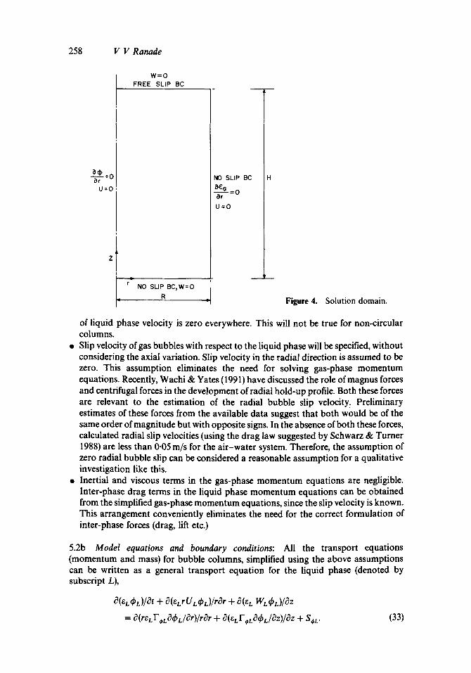
The case of gas-liquid flow in a cylindrical bubble column is considered. The cylindrical co-ordinate system has been used with the origin located at the bottom centre. A schematic diagram of the column with the co-ordinate system is shown in figure 4. In order to highlight the key features of internal circulation in bubble columns, we have eliminated the non-essential aspects from the problem using the following assumptions.

• Gases and liquids are considered incompressible fluids. • The flow has a symmetry in the tangential direction and the tangential component

258 Y V Ranade

a~ "at : 0

U:O

W=O FREE SLIP BC

Z '

NO SLIP BC

~E~ _ O O r -

U = O

i

r NO SLIP BC~W=O

R • Figure 4. Solution domain.

of liquid phase velocity is zero everywhere. This will not be true for non-circular columns.

• Slip velocity of gas bubbles with respect to the liquid phase will be specified, without considering the axial variation. Slip velocity in the radial direction is assumed to be zero. This assumption eliminates the need for solving gas-phase momentum equations. Recently, Wachi & Yates (1991) have discussed the role of magnus forces and centrifugal forces in the development of radial hold-up profile. Both these forces are relevant to the estimation of the radial bubble slip velocity. Preliminary estimates of these forces from the available data suggest that both would be of the same order of magnitude but with opposite signs. In the absence ofboth these forces, calculated radial slip velocities (using the drag law suggested by Schwarz & Turner 1988) are less than 0.05 m/s for the air-water system. Therefore, the assumption of zero radial bubble slip can be considered a reasonable assumption for a qualitative investigation like this.

• Inertial and viscous terms in the gas-phase momentum equations are negligible. Inter-phase drag terms in the liquid phase momentum equations can be obtained from the simplified gas-phase momentum equations, since the slip velocity is known. This arrangement conveniently eliminates the need for the correct formulation of inter-phase forces (drag, lift etc.)

5.2b Model equations and boundary conditions: All the transport equations (momentum and mass) for bubble columns, simplified using the above assumptions can be written as a general transport equation for the liquid phase (denoted by subscript L),

C3(eL ~l,)/t3t + C?(~L rU L dPL)/rt~r + t~(e L WL ~L)/CgZ

= t~(reLF,Lt~q~L/dr)/rt~r + t~(eLF,Lt~d;L/t3Z)/dZ + S,L. (33)

Numer ica l s imulation o f dispersed gas- l iqu id f l o w s

Table 1. The details of equation (33).

259

~b F¢ S~

1 0 U #~ff W #eft k #eff/O'k

where

-- aL d P / d r -- eL d X / d r + F~L

-- e,L~p/t3r + e, LeGg + FzDL G - ¢ ~ ( C 1 G - C 2 ~ ) / k

G = Iz,{2[(dU/dr) 2 + (dW/dz) 2 + (U/r) 2 ] + (dU/dz + dW/dr) 2}

P~fr = Iz + lzr

~t = CDk2 /t~

Model parameters C a -- 0-09 C 1 = 1"43 C 2 = 1-92 trk = 1"0 t L = 1"3 cr~ = 1"0

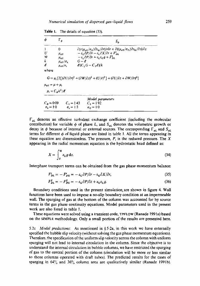
F,L denotes an effective turbulent exchange coefficient (including the molecular contribution) for variable ~ of phase L, and S,L denotes the volumetric growth or decay in ~b because of internal or external sources. The corresponding F,~. and S,~. terms for different ~b of liquid phase are listed in table 1. All the terms appearing in these equation are dimensionless. The pressure, P, is the reduced pressure. The X appearing in the radial momentum equation is the hydrostatic head defined as:

j " H

X = e Lg dz. (34) z

Interphase transport terms can be obtained from the gas phase momentum balance:

FrDL =- - - FrDG = - - E G t~P/t~r - - e a ~ X / d r , (35)

F Z L = - - F Z G -~- - - e a d P /d z + e~eLg. (36)

Boundary conditions used in the present simulation.are shown in figure 4. Wall functions have been used to impose a no-slip boundary condition at an impermeable wall. The sparging of gas at the bottom of the column was accounted for by source terms in the gas phase continuity equations. Model parameters used in the present work are also listed in table 1.

These equations were solved using a transient code, TPFLOW (Ranade 1991 a) based on the SIMPLE methodology. Only a small portion of the results are presented here.

5.2c M o d e l predictions: As mentioned in § 5-2a, in this work we have externally specified the bubble slip velocity (without solving the gas phase momentum equations). Therefore, the specification of the uniform slip velocity across the column with uniform sparging will not lead to internal circulation in the column. Since the objective is to understand the internal circulation in bubble columns, we have restricted the sparging of gas to the central portion of the column (circulation will be more or less similar to those columns operated with draft tubes). The predicted results for the cases of sparging in 64~o and 36~ column area are qualitatively similar (Ranade 1991b).

260 V V Ranade

Therefore, all the results described below (§ 5.2c(i)) are for gas sparging restricted to the central 64% of area. The differences in computed results for 5 x 10, 10 x 20 and 15 x 30 grids are not very significant for the purpose of developing qualitative understanding of the flow system. Therefore, the following results are presented for the 5 × 10 grids unless mentioned otherwise.

5.2c(i) With radially uniform slip velocity. (a) Influence of gas velocity and column diameter-It is necessary to verify that the numerical simulation model correctly predicts the experimentally observed trends in circulation velocity with respect to column diameter and superficial gas velocity. Figure 5 shows the predicted variation of maximum axial velocity with these parameters. It can be seen that column diameter does not affect the average gas hold-up whereas it is almost linearly proportional to the superficial gas velocity. The maximum axial velocity roughly varies with the cube root of diameter and gas velocity. This proves the applicability of the model within the broad range of operation modes, as the trends are represented correctly. Results of some numerical experiments are described below to help determine the sensitive parameters which control and dominate the fluid-dynamic behaviour.

(b) Influence of bubble slip velocity- The imposed bubble slip velocity is one of the key parameters which determine the average gas hold-up and internal circulation in the column. The predicted influence of bubble slip velocity on maximum axial velocity and

0-7

.~ O.E E

E.J

. 0 " 5 :>- b-. U 0

0 .4

x 0.~

~ 0.2

0-1

0.1 0,3 I

COLUMN D I A M E T E R ~ D m

0 .2 0 .3 0.4 0 -5 0.6

ol I i i J f 0.01 0 . 0 5 0 .05 0.07 0 .09 0.1

S U P E R F I C I A L GAS VELOCITY, V G m/s

Figure 5. Trends of variation of the predicted maximum axial velocity and average gas hold-up with respect to column diameter and gas superficial velocity. Column height=column diameter; sparging area=64%; superficial gas velocity = 0-064m/s; axial bubble slip velocity = 0-3075 m/s.

,Y 0_

? 0.2

"l-

J

Z 0

u

0.1 ,,, (.9

w

Numerical simulation of dispersed gas-liquid flows 261

8

" ~ 0 . 7

0 _1 W >

X

~0

m,l -a 0.~ Z 0

Z W

10.6

t~ Q)

0"5

i ,'7 / 0

0 . 4 - r co

0.3 "~ z 0

D.2 ~

0.1

0"5 I I I I 0. ! 0 -2 0 .3 0 . 4

B U B B L E S L I P V E L O C I T Y , V s m/s

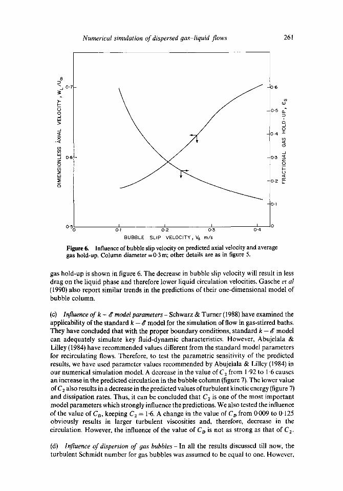
Figure 6. Influence of bubble slip velocity on predicted axial velocity and average gas hold-up. Column diameter =0.3 m; other details are as in figure 5.

gas hold-up is shown in figure 6. The decrease in bubble slip velocity will result in less drag on the liquid phase and therefore lower liquid circulation velocities. Gasche et al (1990) also report similar trends in the predictions of their one-dimensional model of bubble column.

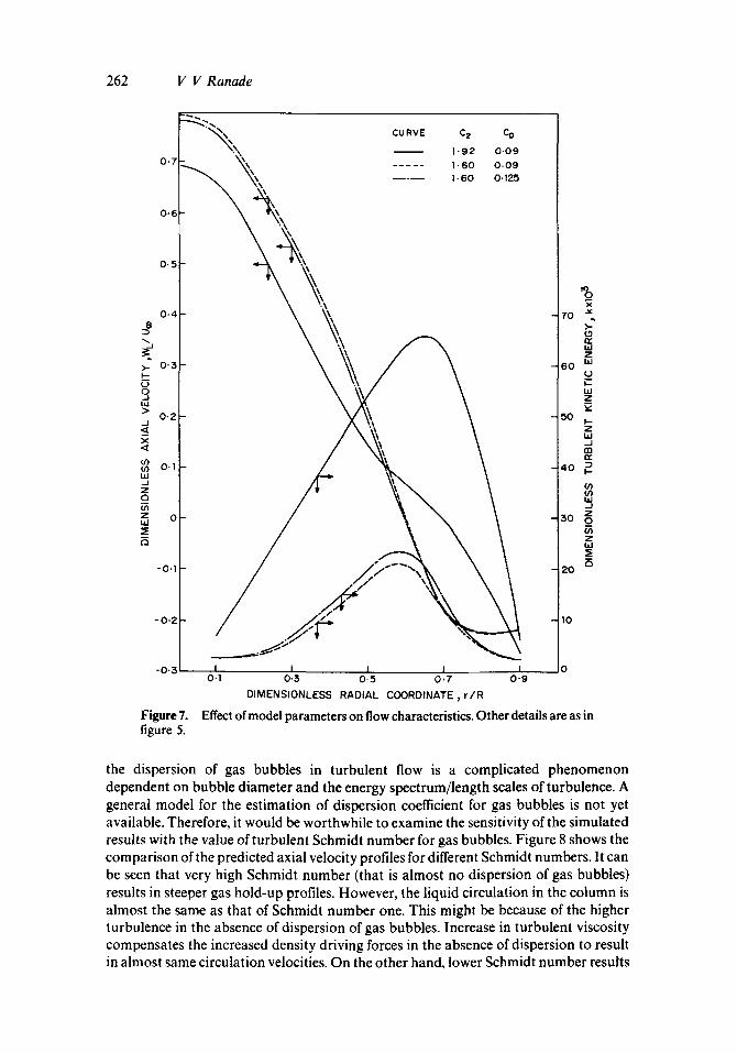
(c) Influence of k - 8 model parameters - Schwarz & Turner (1988) have examined the applicability of the standard k - o ~ model for the simulation of flow in gas-stirred baths. They have concluded that with the proper boundary conditions, standard k - 8 model can adequately simulate key fluid-dynamic characteristics. However, Abujelala & Lilley (1984) have recommended values different from the standard model parameters for recirculating flows. Therefore, to test the parametric sensitivity of the predicted results, we have used parameter values recommended by Abujelala & Lilley (1984) in our numerical simulation model. A decrease in the value of C2 from 1-92 to 1-6 causes an increase in the predicted circulation in the bubble column (figure 7). The lower value of C 2 also results in a decrease in the predicted values of turbulent kinetic energy (figure 7) and dissipation rates. Thus, it can be concluded that C2 is one of the most important model parameters which strongly influence the predictions. We also tested the influence of the value of C o, keeping C2 = 1.6. A change in the value of Co from 0.009 to 0-125 obviously results in larger turbulent viscosities and, therefore, decrease in the circulation. However, the influence of the value of Co is not as strong as that of C 2.

(d) Influence of dispersion of gas bubbles - In all the results discussed till now, the turbulent Schmidt number for gas bubbles was assumed to be equal to one. However,

0 . 7

0 - 6

0 . 5

0 - 4 8

>- 0 - 3

o 3 >

0 . 2 _1

~ 0 . 1 l.d .._1 z 0

z 0 u.I

-0 -1

- 0 ' 2 /

CURVE C 2

1 , 9 2

. . . . . ] , 6 0 | • 6 0

262 V V Ranade

-0 .31 I I I I 0 '1 0"3 0 ' 5 0 . 7

D I M E N S I O N L E S S R A D I A L COORDINATE , r / R

Figure 7. figure 5.

Co

0 . 0 9

0 - 0 9 0-125

7 0 "~

w z

6 0 ~ U

u,l _z v

I.- z w ,_1 a l

4o ~ if)

3o ~ z w

2 0

] 0

I 0 0 " 9

Effect of model parameters on flow characteristics. Other details are as in

the dispersion of gas bubbles in turbulent flow is a complicated phenomenon dependent on bubble diameter and the energy spectrum/length scales of turbulence. A general model for the estimation of dispersion coefficient for gas bubbles is not yet available. Therefore, it would be worthwhile to examine the sensitivity of the simulated results with the value of turbulent Schmidt number for gas bubbles. Figure 8 shows the comparison of the predicted axial velocity profiles for different Schmidt numbers. It can be seen that very high Schmidt number (that is almost no dispersion of gas bubbles) results in steeper gas hold-up profiles. However, the liquid circulation in the column is almost the same as that of Schmidt number one. This might be because of the higher turbulence in the absence of dispersion of gas bubbles. Increase in turbulent viscosity compensates the increased density driving forces in the absence of dispersion to result in almost same circulation velocities. On the other hand, lower Schmidt number results

Numerical simulation of dispersed gas-liquid flows 263

0 " 7

0 . 6

0 . 5

0 . 4

=8 #

0 " 3 >- I - o 3 I,U > 0 " 2 /

X

(/3 O~ 0 -1 la.I _1 Z c2_ (D Z

0

0

N q . \\\\

\\ \

CURVE

1 . 0 I . E 2 0 0 - 1

\ ,

x\\

0"5

(.9 t.D (1. ? t:) ._/ O 1- o~ t9

0.2 . j

z o

h

~ ~ O.1

- O. 1 Xx,

-0.2 ~\ - 0 , 3 I i I I I ~ I J I O

0 . 1 0 - 3 0 " 5 0 , 7 0 . 9

D I M E N S I O N L E S S R A D I A L COORDINATE

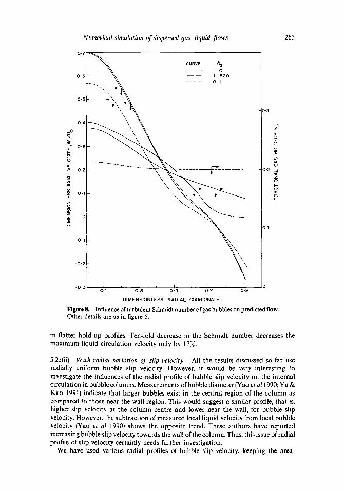
FigureS. Influence of turbulent Schmidt number of gas bubbles on predicted flow. Other details are as in figure 5.

in flatter hold-up profiles. Ten-fold decrease in the Schmidt number decreases the maximum liquid circulation velocity only by 17%.

5.2c(ii) With radial variation of slip velocity. All the results discussed so far use radially uniform bubble slip velocity. However, it would be very interesting to investigate the influences of the radial profile of bubble slip velocity on the internal circulation in bubble columns. Measurements of bubble diameter (Yao et al 1990; Yu & Kim 1991) indicate that larger bubbles exist in the central region of the column as compared to those near the wall region. This would suggest a similar profile, that is, highe= slip velocity at the column centre and lower near the wall, for bubble slip velocity. However, the subtraction of measured local liquid velocity from local bubble velocity (Yao et al 1990) shows the opposite trend. These authors have reported increasing bubble slip velocity towards the wall of the column. Thus, this issue of radial profile of slip velocity certainly needs further investigation.

We have used various radial profiles of bubble slip velocity, keeping the area-

264 V V Ranade

0-@

0 . 6

0"@

CURVE SLIP VELOCITY No. PROFILE

1 - 0.205 D+( r /R?] 2 - - 0 . 1 8 4 5 [ ] ÷ ( r / R ) ] 3 . -- 0 . 3 0 7 5

4 -- 0 . 9 2 2 5 [ 1 - ( r / R ) ] 5 0 - 6 1 5 I ' l - ( r / R ) z ] 6 - 0 . 4 6 1 2 5 r l - ( r / R ) 4 ]

0 . 4

I - t.) 0 0'3 .J LU >

-J

x 0 . 2 <~

(/) (/3 LU /

z O . l 0 (/) z LJJ

a 0

- 0 - 1

- 0 . 2

03 F y \ ' I i I i I t 1 i

0 0 2 0 . 4 0 ' 6 0"9 1-0

D I M E N S I O N L E S S R A D I A L COORDINAT, E , r / R

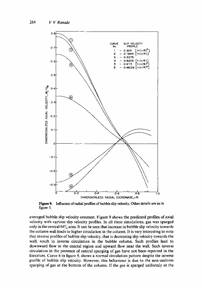
Figure 9. Influence of radial profiles of bubble slip velocity. Other details are as in figure 5.

averaged bubble slip velocity constant. Figure 9 shows the predicted profiles of axial velocity with various slip velocity profiles. In all these simulations, gas was sparged only in the central 64% area. It can be seen that increase in bubble slip velocity towards the column wall leads to higher circulation in the column. It is very interesting to note that inverse profiles of bubble slip velocity, that is decreasing slip velocity towards the wall, result in inverse circulation in the bubble column. Such profiles lead to downward flow in the central region and upward flow near the wall. Such inverse circulation in the presence of central sparging of gas have not been reported in the literature. Curve 6 in figure 9, shows a normal circulation pattern despite the inverse profile of bubble slip velocity. However, this behaviour is due to the non-uniform sparging of gas at the bottom of the column. If the gas is sparged uniformly at the

Numerical simulation of dispersed 9as-liquid flows 265

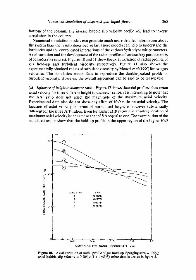
bottom of the column, any inverse bubble slip velocity profile will lead to inverse circulation in the column.

Numerical simulation models can generate much more detailed information about the system than the results described so far. These models can help to understand the intricacies and the complicated interactions of the various hydrodynamic parameters. Axial variation and the development of the radial profiles of various key parameters is of considerable interest. Figures 10 and 11 show the axial variation of radial profiles of gas hold-up and turbulent viscosity respectively. Figure 11 also shows the experimentally obtained values of turbulent viscosity by Menzel et al (1990) for two gas velocities. The simulation model fails to reproduce the double-peaked profile of turbulent viscosity. However, the overall agreement can be said to be reasonable.

(a) Influence of height to diameter ratio - Figure 12 shows the axial profiles of the mean axial velocity for three different height to diameter ratios. It is interesting to note that the H/D ratio does not affect the magnitude of the maximum axial velocity. Experimental data also do not show any affect of H/D ratio on axial velocity. The location of axial velocity in terms of normalised height is however substantially different for the three H/D ratios. Even for higher H/D ratios, the absolute location of maximum axial velocity is the same as that of H/D equal to one. The examination of the simulated results show that the hold-up profile in the upper region of the higher H/D

0 ' 3

(.9 t,O

0 " 2 O_

.J 0 -1-

03 <{ (,9 .J < z 0 r- o.1 (J n~ h

CURVE No. Z / H ! 0 . 0 2 5 2 0 . 3 ' 7 5 3 0 " 6 7 , 5 4 0 . 9 7 5

I O I t I i l I I I I I

0 . 2 0 - 4 0 ' 6 0 . 6 ] ,0

D I M E N S I O N L E S S R A D I A L COORDINATE ~ r / R

Figure 10. Axial variation of radial profile of gas hold-up. Sparging area = 100%; axial bubble slip velocity = 0.205 x (1 + (r/R)2); other details are as in figure 5.

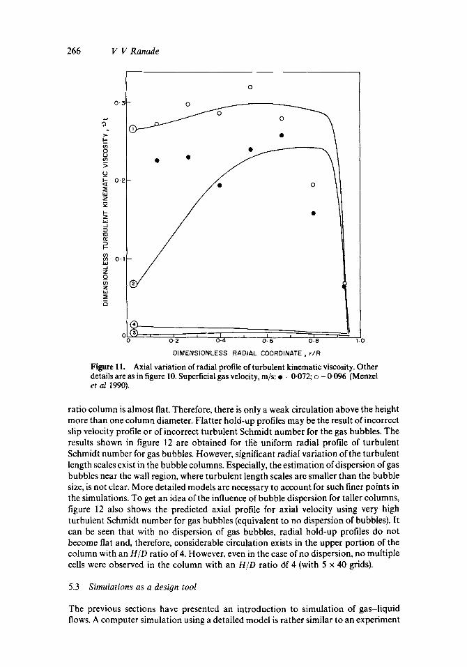
266 V V Ranade

>.- (/) 0 C.)

(,..)

~E kl.I Z

I - Z ILl

rn n~

lIJ -J Z _o

Z ~J

0"~

0 " 2

0 - !

( ~ , J I I 0 0 - 2 0 . 4 0 . 6 0 ! 8 1 .0

O

, : ~ _ . . . j J o o

DIMENSIONLESS RADIAL COORDINATE, r/R

Figure 11. Axial variation of radial profile of turbulent kinematic viscosity. Other details are as in figure 10. Superficial gas velocity, m/s: • - 0.072; o - 0.096 (Menzei et al 1990).

ratio column is almost fiat. Therefore, there is only a weak circulation above the height more than one column diameter. Flatter hold-up profiles may be the result of incorrect slip velocity profile or of incorrect turbulent Schmidt number for the gas bubbles. The results shown in figure 12 are obtained for ttie uniform radial profile of turbulent Schmidt number for gas bubbles. However, significant radial variation of the turbulent length scales exist in the bubble columns. Especially, the estimation of dispersion of gas bubbles near the wall region, where turbulent length scales are smaller than the bubble size, is not clear. More detailed models are necessary to account for such finer points in the simulations. To get an idea of the influence of bubble dispersion for taller columns, figure 12 also shows the predicted axial profile for axial velocity using very high turbulent Schmidt number for gas bubbles (equivalent to no dispersion of bubbles). It can be seen that with no dispersion of gas bubbles, radial hold-up profiles do not become flat and, therefore, considerable circulation exists in the upper portion of the column with an H/D ratio of 4. However, even in the case of no dispersion, no multiple cells were observed in the column with an H/D ratio df 4 (with 5 x 40 grids).

5.3 Simulations as a desi#n tool

The previous sections have presented an introduction to simulation of gas-liquid flows. A computer simulation using a detailed model is rather similar to an experiment

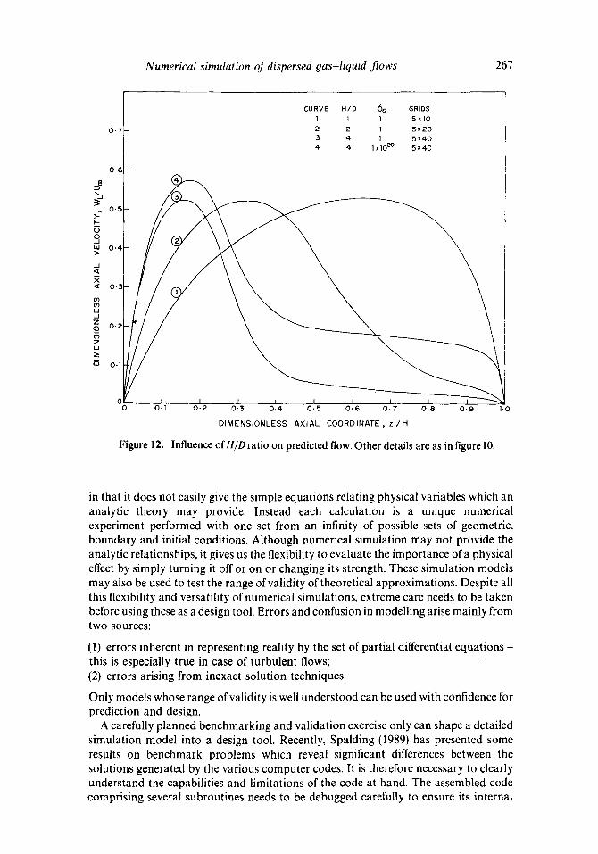
Numerical simulation of dispersed gas-liquid flows 267

I..-

q w >

<

if) if) bJ ...I Z O

Z W

t CURVE H/D 6 G GRIDS I ] l 5xlO

0-7 2 2 I 5x20 3 4 | 5x40 4 4 lxlO 20 5x40

0,6

0.5

0-4

0-3

0-2

0-1

0 0 0.1 0"2 0"3 0.4 0.5 0.6 0.7 0 '8 0.9 1.0

DIMENSIONLESS AXIAL COORDINATE~ z / H

Figure 12. Influence of H/D ratio on predicted flow. Other details are as in figure 10.

in that it does not easily give the simple equations relating physical variables which an analytic theory may provide. Instead each calculation is a unique numerical experiment performed with one set from an infinity of possible sets of geometric, boundary and initial conditions. Although numerical simulation may not provide the analytic relationships, it gives us the flexibility to evaluate the importance of a physical effect by simply turning it off or on or changing its strength. These simulation models may also be used to test the range of validity of theoretical approximations. Despite all this flexibility and versatility of numerical simulations, extreme care needs to be taken before using these as a design tool. Errors and confusion in modelling arise mainly from two sources:

(1) errors inherent in representing reality by the set of partial differential equations - this is especially true in case of turbulent flows; (2) errors arising from inexact solution techniques.

Only models whose range of validity is well understood can be used with confidence for prediction and design.

A carefully planned benchmarking and validation exercise only can shape a detailed simulation model into a design tool. Recently, Spalding (1989) has presented some results on benchmark problems which reveal significant differences between the solutions generated by the various computer codes. It is therefore necessary to clearly understand the capabilities and limitations of the code at hand. The assembled code comprising several subroutines needs to be debugged carefully to ensure its internal

268 V V Ranade

connections and correct operation. This is an especially hard task when the code is churning out physically realistic results. Oran & Boris (1987) have discussed these issues excellently in a recent book (though for single-phase flows) and suggested some ways to avoid common pitfalls in numerical simulation.

6. Summary

Major aspects of numerical simulation of gas-liquid dispersed flows have been discussed. Formulation of various transport equations and corresponding phenomenological models have been presented. Emphasis has been laid on describing numerical techniques and algorithms for constructing CFD simulation codes for two- phase flows. Though greater attention has been paid to dispersed gas-liquid flows, the methodology can be applied to any multi-phase problem. Special features of multi- phase flow simulation over single-phase simulation have been highlighted.

A case of gas-liquid flow in a bubble column is presented as an illustration for the general methodology. Simulated mean flow fields agree reasonably with the experimental data. Properly validated CFD codes thus can serve as a useful tool for design engineers of multi-phase systems. Some of the common pitfalls in using simulation codes for design have also discussed. This review is expected to give an overall idea about the present state of art of two-phase simulation in industrial equipment. Some suggestions for further work have also been made below.

7. Suggestions for further work

Because of the practical manifestations of multi-phase flow phenomena, we hope that powerful tools like the CFD codes will be widely used. Before closing this review, it would therefore be useful to look into some obstacles to the complete success of the CFD approach.

First of all, incompletely solved problems of single-phase numerical fluid mechanics spread their influence in the multi-phase area. Some of these can be listed as:

• how to conduct fine-grid computations cheaply; • how to minimise numerical diffusion without jeopardizing the robustness of the CFD code; • how to preserve order and flexibility in CFD codes as the complexity of their physical content increases.

These problems are of a computational character. Those of a physical character primarily concern the search for reaiistic and universal turbulence models. More work is necessary to understand various ways in which a dispersed phase influences the turbulence properties of continuous phase. The transport of the dispersed phase due to the turbulence in continuous phase and its dependence on the size of the dispersed phase needs to be studied in detail. Inter-phase transfer laws also need to be improved. Comprehensive experimental programs need to be planned to develop such an understanding. The interaction between accurate measurements using better experimental techniques and mathematical modelling of various unknown terms can only lead to better simulation models and codes.

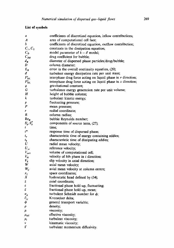
Numerical simulation of dispersed gas-liquid flows 269

List of symbols

a

A b C 1 , C 2

CD CoB dB D ER 8 FS,~ F~,L g G H k P P r

R Res s;,s t t* te tk U Uo~ I/cell

v,. Vs W w,: Xj X

g

¢3~ i

P I z ,LLeff ~t "V

F

coefficients of discretized equation, inflow contributions; area of computational cell face; coefficients of discretized equation, outflow contribution; constants in the dissipation equation; model parameter of k - ~ model; drag coefficient for bubble; diameter of dispersed phase particles/drop/bubble; column diameter; error in the overall continuity equation, (20); turbulent energy dissipation rate per unit mass; interphase drag force acting on liquid phase in r direction; interphase drag force acting on liquid phase in z direction; gravitational constant; turbulence energy generation rate per unit volume; height of bubble column; turbulent kinetic energy; fluctuating pressure; mean pressure; radial coordinate; column radius; bubble Reynolds number; components of source term, (27); time; response time of dispersed phase; characteristic time of energy containing eddies; characteristic time of dissipating eddies; radial mean velocity; reference velocity; volume of computational cell; velocity of kth phase in i direction; slip velocity in axial direction; axial mean velocity; axial mean velocity at column centre; space coordinates; hydrostatic head defined by (34); axial coordinate; fractional phase hold-up, fluctuating; fractional phase hold-up, mean; turbulent Schmidt number for 4); Kronecker delta; general transport variable; density; viscosity; effective viscosity; turbulent viscosity; kinematic viscosity; turbulent momentum diffusivity.

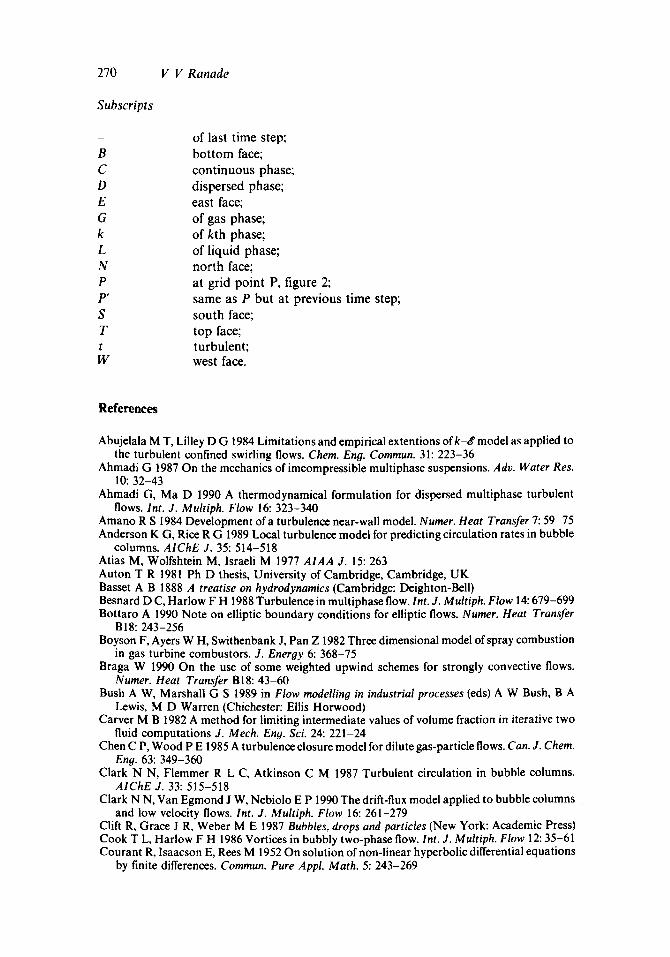
270 V V Ranade

Subscripts

- of last time step; B bottom face; C continuous phase; D dispersed phase; E east face; G of gas phase; k of kth phase; L of liquid phase; N north face; P at grid point P, figure 2; P' same as P but at previous time step; S south face; T top face; t turbulent; W west face.

R e f e r e n c e s

Abujelala M T, Lilley D G 1984 Limitations and empirical extentions of k-8 model as applied to the turbulent confined swirling flows. Chem. Eng. Commun. 31:223-36

Ahmadi G 1987 On the mechanics of imcompressible multiphase suspensions. Adv. Water Res. 10:32-43

Ahmadi G, Ma D 1990 A thermodynamical formulation for dispersed multiphase turbulent flows. Int. J. Multiph. Flow 16:323-340

Amano R S 1984 Development of a turbulence near-wall model. Numer. Heat Transfer 7:59-75 Anderson K G, Rice R G 1989 Local turbulence model for predicting circulation rates in bubble

columns. AIChE J. 35:514-518 Atias M, Wolfshtein M, Israeli M 1977 AIAA J. 15:263 Auton T R 1981 Ph D thesis, University of Cambridge, Cambridge, UK Basset A B 1888 A treatise on hydrodynamics (Cambridge: Deighton-Bell) Besnard D C, Harlow F H 1988 Turbulence in multiphase flow. Int. J. Multiph. Flow 14:679-699 Bottaro A 1990 Note on elliptic boundary conditions for elliptic flows. Numer. Heat Transfer

B18:243-256 Boyson F, Ayers W H, Swithenbank J, Pan Z 1982 Three dimensional model of spray combustion

in gas turbine combustors. J. Energy 6:368-75 Braga W 1990 On the use of some weighted upwind schemes for strongly convective flows.

Numer. Heat Transfer B18:43-60 Bush A W, Marshall G S 1989 in Flow modelling in industrial processes (eds) A W Bush, B A

Lewis, M D Warren (Chichester: Ellis Horwood) Carver M B 1982 A method for limiting intermediate values of volume fraction in iterative two

fluid computations J. Mech. Eng. Sci. 24:221-24 Chen C P, Wood P E 1985 A turbulence closure model for dilute gas-particle flows. Can. J. Chem.

Eng. 63:349-360 Clark N N, Flemmer R L C, Atkinson C M 1987 Turbulent circulation in bubble columns.

AIChE J. 33:515-518 Clark N N, Van Egmond J W, Nebioio E P 1990 The drift-flux model applied to bubble columns

and low velocity flows. Int. J. Multiph. Flow 16:261-279 Clift R, Grace J R, Weber M E 1987 Bubbles, drops and particles (New York: Academic Press) Cook T L, Harlow F H 1986 Vortices in bubbly two-phase flow. Int. J. Multiph. Flow 12:35-61 Courant R, Isaacson E, Rees M 1952 On solution of non-linear hyperbolic differential equations

by finite differences. Commun. Pure Appl. Math. 5:243-269

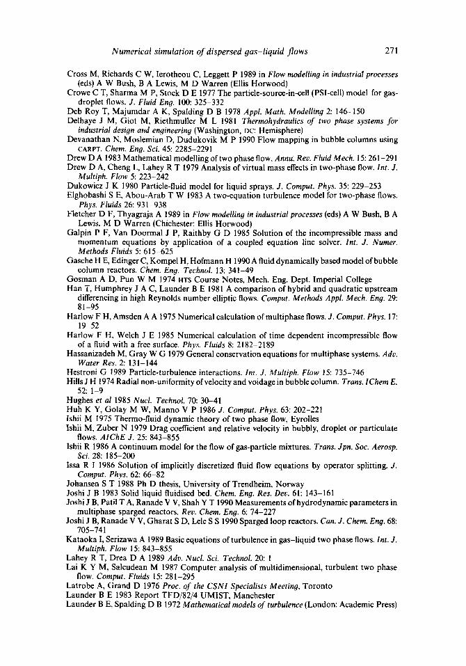
Numerical simulation of dispersed gas-liquid flows 271

Cross M, Richards C W, lerotheou C, Leggett P 1989 in Flow modelling in industrial processes (eds) A W Bush, B A Lewis, M D Warren (Ellis Horwood)

Crowe C T, Sharma M P, Stock D E 1977 The particle-source-in-cell (PSI-cell) model for gas- droplet flows. J. Fluid Eng. 100:325-332

Deb Roy T, Majumdar A K, Spalding D B 1978 Appl. Math. Modelling 2:146-150 Delhaye J M, Giot M, Riethmuller M L 1981 Thermohydraulics of two phase systems for

industrial design and engineering (Washington, DC: Hemisphere) Devanathan N, Moslemian D, Dudukovik M P 1990 Flow mapping in bubble columns using

CARPT. Chem. Eng. Sci. 45:2285-2291 Drew D A 1983 Mathematical modelling of two phase flow. Annu: Rev. Fluid Mech. 15:261-291 Drew D A, Cheng L, Lahey R T 1979 Analysis of virtual mass effects in two-phase flow. Int. J.

Multiph. Flow 5:223-242 Dukowicz J K 1980 Particle-fluid model for liquid sprays. J. Comput. Phys. 35:229-253 Elghobashi S E, Abou-Arab T W 1983 A two-equation turbulence model for two-phase flows.

Phys. Fluids 26:931-938 Fletcher D F, Thyagraja A 1989 in Flow modelling in industrial processes (eds) A W Bush, B A

Lewis, M D Warren (Chichester: Ellis Horwood) Galpin P F, Van Doormal J P, Raithby G D 1985 Solution of the incompressible mass and

momentum equations by application of a coupled equation line solver. Int. J. Numer. Methods Fluids 5:615-625

Gasche H E, Edinger C, Kompel H, Hofmann H 1990 A fluid dynamically based model of bubble column reactors. Chem. Eng. Technol. 13:341-49

Gosman A D, Pun W M 1974 HTS Course Notes, Mech. Eng. Dept. Imperial College Hun T, Humphrey J A C, Launder B E 1981 A comparison of hybrid and quadratic upstream

differencing in high Reynolds number elliptic flows. Comput. Methods Appl. Mech. Eng. 29: 81-95

Harlow F H, Amsden A A 1975 Numerical calculation of multiphase flows. J. Comput. Phys. 17: 19-52

Harlow F H, Welch J E 1985 Numerical calculation of time dependent incompressible flow of a fluid with a free surface. Phys. Fluids 8:2182-2189

Hassanizadeh M, Gray W G 1979 General conservation equations for muitiphase systems. Adv. Water Res. 2:131-144

Hestroni G 1989 Particle-turbulence interactions. Int. J. Multiph. Flow 15:735-746 Hills J H 1974 Radial non-uniformity of velocity and voidage in bubble column. Trans. IChem E.

52:1-9 Hughes et al 1985 Nucl. Technol. 70:30-41 Huh K Y, Golay M W, Manno V P 1986 J. Comput. Phys. 63" 202-221 Ishii M 1975 Thermo-fluid dynamic theory of two phase flow, Eyrolles lshii M, Zuber N 1979 Drag coefficient and relative velocity in bubbly, droplet or particulate

flows. AIChE J. 25:843-855 Ishii R 1986 A continuum model for the flow of gas-particle mixtures. Trans. Jpn. Soc. Aerosp.

Sci. 28:185-200 Issa R I 1986 Solution of implicitly discretized fluid flow equations by operator splitting. J.

Comput. Phys. 62:66-82 Johansen S T 1988 Ph D thesis, University of Trendheim, Norway Joshi J B 1983 Solid liquid fluidised bed. Chem. Eng. Res. Dev. 61:143-161 Joshi J B, Patil T A, Ranade V V, Shah Y T 1990 Measurements of hydrodynamic parameters in

multiphase sparged reactors. Rev. Chem. Eng. 6:74-227 Joshi J B, Ranade V V, Gharat S D, Lele S S 1990 Sparged loop reactors. Can. J. Chem. Eng. 68:

705-741 Kataoka I, Serizawa A 1989 Basic equations of turbulence in gas-liquid two phase flows. Int. J.

Multiph. Flow 15:843-855 Lahey R T, Drea D A 1989 Adv. Nucl. Sci. Technol. 20:1 Lai K Y M, Salcudean M 1987 Computer analysis of multidimensional, turbulent two phase

flow. Comput. Fluids 15:281-295 Latrobe A, Grand D 1976 Proc. of the CSNI Specialists Meeting, Toronto Launder B E 1983 Report TFD/82/4 UMIST, Manchester Launder B E, Spalding D B 1972 Mathematical models of turbulence (London: Academic Press)

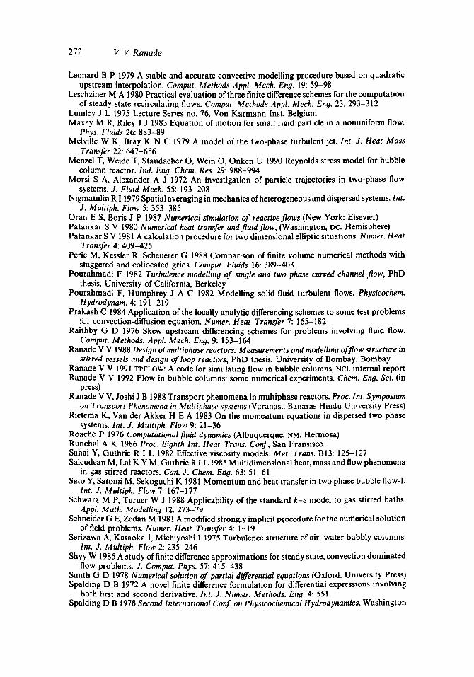
272 V V Ranade

Leonard B P 1979 A stable and accurate convective modelling procedure based on quadratic upstream interpolation. Comput. Methods Appl. Mech. Eng. 19:59-98

Leschziner M A 1980 Practical evaluation of three finite difference schemes for the computation of steady state recirculating flows. Comput. Methods Appl. Mech. Eng. 23:293-312

Lumley J L 1975 Lecture Series no. 76, Von Karmann Inst. Belgium Maxey M R, Riley J J 1983 Equation of motion for small rigid particle in a nonuniform flow.

Phys. Fluids 26:883-89 Melville W K, Bray K N C 1979 A model of.the two-phase turbulent jet. Int. J. Heat Mass

Transfer 22:647-656 Menzel T, Weide T, Staudacher O, Wein O, Onken U 1990 Reynolds stress model for bubble

column reactor. Ind. En#. Chem. Res. 29:988-994 Morsi S A, Alexander A J 1972 An investigation of particle trajectories in two-phase flow

systems. J. Fluid Mech. 55:193-208 Nigmatulin R I 1979 Spatial averaging in mechanics of heterogeneous and dispersed systems. Int.

J. Multiph. Flow 5:353-385 Oran E S, Boris J P 1987 Numerical simulation of reactive flows (New York: Elsevier) Patankar S V 1980 Numerical heat transfer and fluid flow, (Washington, PC: Hemisphere) Patankar S V 1981 A calculation procedure for two dimensional elliptic situations. Numer. Heat

Transfer 4:409-425 Peric M, Kessler R, Scheuerer G 1988 Comparison of finite volume numerical methods with

staggered and collocated grids. Comput. Fluids 16:389-403 Pourahmadi F 1982 Turbulence modelling of single and two phase curved channel flow, PhD

thesis, University of California, Berkeley Pourahmadi F, Humphrey J A C 1982 Modelling solid-fluid turbulent flows. Physicochem.

Hydrodynam. 4:191-219 Prakash C 1984 Application of the locally analytic differencing schemes to some test problems

for convection-diffusion equation. Numer. Heat Transfer 7:165-182 Raithby G D 1976 Skew upstream differencing schemes for problems involving fluid flow.

Comput. Methods. Appl. Mech. Eng. 9:153-164 Ranade V V 1988 Design of multiphase reactors: Measurements and modelling of flow structure in

stirred vessels and design of loop reactors, PhD thesis, University of Bombay, Bombay Ranade V V 1991 TPFLOW: A code for simulating flow in bubble columns, NCL internal report Ranade V V 1992 Flow in bubble columns: some numerical experiments. Chem. Eng. Sci. (in

press) Ranade V V, Joshi J B 1988 Transport phenomena in multiphase reactors. Proc. Int. Symposium

on Transport Phenomena in Multiphase systems (Varanasi: Banaras Hindu University Press) Rietema K, Van der Akker H E A 1983 On the momeatum equations in dispersed two phase

systems. Int. J. Multiph. Flow 9:21-36 Roache P 1976 Computationalfluid dynamics (Albuquerque, NM: Hermosa) Runchal A K 1986 Proc. Eighth Int. Heat Trans. Conf., San Fransisco Sahai Y, Guthrie R I L 1982 Effective viscosity models. Met. Trans. BI3:125-127 Salcudean M, Lai K Y M, Guthrie R I L 1985 Multidimensional heat, mass and flow phenomena

in gas stirred reactors. Can. J. Chem. Eng. 63:51-61 Sato Y, Satomi M, Sekoguchi K 1981 Momentum and heat transfer in two phase bubble flow-I.

Int. J. Multiph. Flow 7:167-177 Schwarz M P, Turner W J 1988 Applicability of the standard k-e model to gas stirred baths.

Appl. Math. Modelling 12:273-79 Schneider G E, Zedan M 1981 A modified strongly implicit procedure for the numerical solution

of field problems. Numer. Heat Transfer 4:1-19 Serizawa A, Kataoka I, Michiyoshi I 1975 Turbulence structure of air-water bubbly columns.

Int. J. Multiph. Flow 2:235-246 Shyy W 1985 A study of finite difference approximations for steady state, convection dominated

flow problems. J. Comput. Phys. 57:415-438 Smith G D 1978 Numerical solution of partial differential equations (Oxford: University Press) Spalding D B 1972 A novel finite difference formulation for differential expressions involving

both first and second derivative. Int. J. Numer. Methods. Eng. 4:551 Spalding D B 1978 Second International Conf. on Physicochemical Hydrodynamics, Washington

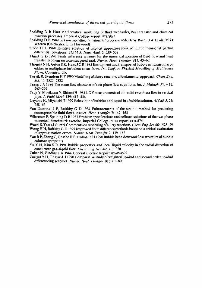
Numerical simulation of dispersed gas-liquid flows 273

Spalding D B 1980 Mathematical modelling of fluid mechanics, heat transfer and chemical reaction processes. Imperial College report HTS/80/1

Spalding D B 1989 in Flow modelling in industrial processes (eds) A W Bush, B A Lewis, M D Warren (Chichester: Ellis Horwood)

Stone H L 1968 Iterative solution of implicit approximations of multidimensional partial differential equations. SIAM J. Num. Anal. 5:530--538

Thiart G D 1990 Finite difference schemes for the numerical solution of fluid flow and heat transfer problem on non-staggered grid. Numer. Heat Transfer BI7:43-62

Thomas N H, Auton S K, Hunt J C R 1983. Entrapment and transport of bubble in transient large eddies in muitiphase turbulent shear flows. Int. Conf. on Physical Modelling of Multiphase Flows, Coventry, UK

Torvik R, Svendsen H F 1990 Modelling of slurry reactors, a fundamental approach. Chem. Eng. Sci. 45:2325-2332

Trapp J A 1986 The mean flow Character of two-phase flow equations. Int. J. Multiph. Flow 12: 263-276

Tsuji Y, Morikawa Y, Shiomi H 1984 LDV measurements of air-solid two phase flow in vertical pipe: J. Fluid Mech 139:417-434

Ueyama K, Miyaudai T 1979 Behaviour of bubbles and liquid in a bubble column. AIChE J. 25" 258-65

Van Doormal J P, Raithby G D 1984 Enhancements of the SIMPLE method for predicting incompressible fluid' flows. Numer. Heat Transfer 7:147-163

Villasenor F, Spalding D B 1987 Problem specifications and collated solutions of the two-phase numerical benchmark exercise, Imperial College CFDU report CrD/87/1

Wachi S, Yates J G 1991 Comments on modelling of slurry reactions. Chem. Eng. Sci. 46:1528-29 Wong H H, Raithby G D 1979 Improved finite difference methods based on a critical evaluation

of approximation errors. Numer. Heat Transfer 2:139-163 Yao B P, Zheng C, Gasche H E, Hofmann H 1990 Bubble behaviour and flow structure of bubble

columns (preprint) Yu Y H, Kim S D 1991 Bubble properties and local liquid velocity in the radial direction of

concurrent gas-liquid flow. Chem. Eng. Sci. 46:313-320 Zuber N, Findlay J A 1964 General Electric Report GEAP-4592 Zurigat Y H, Ghajar A J 1990 Comparative study ofweighted upwind and second order upwind

differenceing schemes. Numer. Heat Transfer BI8:61-80