numerical simulation and economic design of …...1 numerical simulation and economic design of...
TRANSCRIPT

1
Numerical Simulation and Economic Design of Concrete Shear Walls
Reinforced with GFRP Bars
by
Fereshte Talaei
A thesis submitted in partial fulfillment of the requirements for the degree of
Master of Science
in
Structural Engineering
Department of Civil and Environmental Engineering
University of Alberta
© Freshte Talaei, 2017

ii
Abstract
Premature corrosion of reinforcing steel is a cause of concern for steel-reinforced concrete
structures, since it causes them to deteriorate before their design operational life is attained. The
Use of fiber-reinforced polymer (FRP) bars in reinforced-concrete (RC) structures has been shown
to be an effective alternative to mitigate the corrosion problems that occur in steel-reinforced
structures subjected to chemical attack or adverse environmental conditions, such as parkade slabs
and bridge superstructures. However, the high price, limited design knowledge, and uncertainty
about long-term performance in FRP-reinforced structures have prevented widespread use of this
type of reinforcement in civil infrastructure, despite its potential advantages over conventional
steel.
To address these problems, this study presents an investigation in the economic design of FRP-
reinforced concrete shear walls considering typical design constraints found in practice. Shear
walls were chosen due to their important role in providing stiffness and strength to RC buildings,
with FRP reinforcement being an attractive option to provide these elements with a superior
durability than steel, while having a comparable performance in non-seismic areas. Thus, the
study objective is to show how FRP can be used as an economic and efficient alternative to
conventional steel reinforcement in shear wall structures.
To examine the feasible design scenarios in which FRP can be used to have a comparable
performance to that of steel reinforcement, a finite-element analysis model for FRP-reinforced
concrete walls is developed and validated with experimental results. The model was validated with
the test data obtained from three mid-rise FRP-reinforced walls tested at the University of
Sherbrooke in 2013. After validation, the model is used to assess the design scenarios in which
iii
FRP can be used at minimum cost considering variables such as strength, deflection, cracking,
long-term creep, and cost. The governing design constraints create a feasible zone in a diagram of
longitudinal reinforcement vs. wall width. For comparison, a similar analysis is performed for
conventional, steel-reinforced shear walls. It was found that in FRP-reinforced shear walls, due to
the relatively high flexibility of the FRP material, deflections and crack width constraints at service
conditions govern the feasible zone. However, in steel reinforced shear walls the strength
constraint is the governing constraint instead of deflection for the design scenarios considered in
the study. Although there is a notable difference between the initial price of steel and FRP bars,
the optimal design scenario solution for the shear walls reinforced with FRP reinforcement is only
slightly more expensive than the flexural optimal solutions for the steel-reinforced shear walls,
with FRP-reinforced structures having comparable (or superior) strength, deformation capacity,
and cracking resistance than their steel-reinforced counterparts.
Keywords— shear walls; FRP; design; model; concrete; cost-optimization

iv
Dedication
Dedicated to my parents for all the support they gave me without which my academic
achievement would not be possible.

v
Acknowledgement
A part of this research was funded by Natural Sciences and Engineering Research Council,
NSERC, of Canada.
I like to thank my supervisor, Dr. Carlos Cruz Noguez, for his support of this research. His
encouragement, guidance and support from the initial steps of this program enabled me to develop
my understanding of the structural engineering concepts and to carry out the research. He
constantly challenged me to higher standards by reviewing my work and providing me with
feedback. It was a pleasure working in his research team and learning from his vast knowledge
and experiences.
Also, I would like to express my gratitude to my thesis examination committee members, Dr.
Vivek Bindiganavile and Dr. Douglas Tomlinson, for their invaluable thoughts on this thesis.
Last but not least, I would like to thank all my friends and colleagues at the Structural Engineering
group at University of Alberta for their help and support. I extend my appreciation to Seyed
Mobeen, Mohammad Javad Tolou Kian, Nabi Goudarzi and Nima Mohajerrahbari for the time
and effort they put for helping me without which it would not be possible for me to finish this
work.

vi
Contents
1. Chapter 1. Introduction ........................................................................................................................ 1
1.1. Problem Statement ........................................................................................................................ 1
1.2. Objectives and Scope .................................................................................................................... 2
1.3. Methodology ................................................................................................................................. 3
1.4. Thesis Outline ............................................................................................................................... 4
2. Chapter 2. Literature Review ............................................................................................................... 5
2.1. FRP Reinforcement ....................................................................................................................... 5
2.2. Types of FRP Bars ........................................................................................................................ 6
2.3. Properties of FRP Bars .................................................................................................................. 8
2.4. Reinforced Concrete Shear Walls ............................................................................................... 10
2.5. Finite Element Modeling of Reinforced Concrete Structures ..................................................... 12
2.6. Economic Design of Reinforced Concrete Structures ................................................................ 13
3. Chapter 3. Finite Element Analysis ................................................................................................... 18
3.1. Finite-Element Software ............................................................................................................. 18
3.2. Experimental Investigation on GFRP-Reinforced Concrete Walls ............................................. 19
3.2.1. Concrete Dimensions and Reinforcement Configurations of the Shear Wall Specimens .. 19
3.2.2. Material Properties .............................................................................................................. 25
3.2.3. Loading ............................................................................................................................... 26
3.3. VecTor2 Modeling Process ......................................................................................................... 27
3.3.1. Models for Concrete............................................................................................................ 29
3.3.2. Models for GFRP Reinforcement ....................................................................................... 29
3.3.3. Models for Bond ................................................................................................................. 30
3.3.4. Element Library .................................................................................................................. 31
3.4. Analytical Analysis Results (VecTor2) ...................................................................................... 40
4. Chapter 4. Economic Design of FRP-Reinforced RC Shear Walls ................................................... 46
4.1. Background ................................................................................................................................. 46
4.2. Width/Depth vs. Reinforcement Ratio Diagram ......................................................................... 46
4.3. Example Shear Wall Building..................................................................................................... 47

vii
4.4. Reference Wall ............................................................................................................................ 51
4.5. Design Constraints ...................................................................................................................... 54
4.5.1. Ultimate Strength ................................................................................................................ 54
4.5.2. Bar Fracture ........................................................................................................................ 58
4.5.3. Deflection at Service Condition .......................................................................................... 65
4.5.4. Crack Width at Service Condition ...................................................................................... 70
4.5.5. Creep ................................................................................................................................... 74
4.5.6. Cost Function ...................................................................................................................... 79
4.5.7. High Strength Concrete ....................................................................................................... 85
4.5.8. Sensitivity Study of Deflection ........................................................................................... 90
4.5.9. Bond .................................................................................................................................... 92
4.6. Shear Walls with Other Heights, Reinforcement Configurations and Axial Loads .................... 96
5. Chapter 5. Economic Design of Steel-Reinforced RC Shear Walls .................................................. 98
5.1. GFRP Reinforced Shear Walls against Walls with Steel Reinforcement ................................... 98
5.2. Strength Constraint for Steel Reinforced Shear Walls ................................................................ 98
5.3. Minimum and Balanced Reinforcement Ratios for Steel Reinforced Shear Walls .................. 101
5.4. Deflection Constraint for Steel Reinforced Shear Walls .......................................................... 104
5.5. Crack Width Constraint for Steel Reinforced Shear Walls ....................................................... 105
5.6. Cost Function for Steel Reinforced Concrete Shear Walls ....................................................... 107
6. Chapter 6. Summary and Conclusions ............................................................................................. 110
6.1. Summary ................................................................................................................................... 110
6.2. Conclusions ............................................................................................................................... 111
6.3. Recommendations for Future Work .......................................................................................... 113
References ................................................................................................................................................. 114
viii
List of Tables
Table 2. 1: Mechanical properties of reinforcing bars (ACI 440.1R 2006) .................................................. 7
Table 3. 1: Reinforcement ratios of GFRP reinforced shear walls ............................................................. 25
Table 3. 2: Material properties of reinforcement ........................................................................................ 25
Table 3. 3: Elements in VecTor2 library ..................................................................................................... 31
Table 3. 4: Comparison of the different types of reinforcement modeling (G10 wall) .............................. 32
Table 3. 5: Capacities of the GFRP reinforced concrete shear walls (kN) ................................................. 40
Table 4. 1: Material properties of reinforcement ........................................................................................ 50
Table 4. 2: Values for variable (1998) .................................................................................................. 75
Table 4. 3: Material costs ............................................................................................................................ 80
Table 4. 4: Comparison of the optimal design solution costs (GFRP reinforced shear walls) ................... 95
Table 5. 1: Comparison of the optimal design solution costs (GFRP and Steel reinforced shear walls) .. 109
ix
List of Figures
Figure 2. 1: FRP bars .................................................................................................................................... 6
Figure 2. 2: Stress- Strain curves for steel and FRPs .................................................................................... 7
Figure 2. 3: Various GFRP reinforcing bars (ACI 440.1R 2006) ................................................................. 8
Figure 2.4: FRP bars; (a) wrapped and sand-coated; (b) sand-coated; (c) ribbed (ACI 440.1R 2006) ....... 10
Figure 2. 5: Failure modes of shear walls; (a) loading; (b) flexural failure; (c) shear failure; (d) sliding shear
(e) anchorage slip failure (Paulay 1988) ..................................................................................................... 11
Figure 2. 6: Beam cross section (Yousef A Al-Salloum and,Ghulam Husainsiddiqi 1994) ....................... 14
Figure 2. 7: Feasible zone and optimal design solution (Yousef A Al-Salloum and,Ghulam Husainsiddiqi
1994) ........................................................................................................................................................... 15
Figure 2. 8: Structural configuration of the studied T- beam (Balafas and Burgoyne 2012) ...................... 17
Figure 2. 9: Feasible zone and optimal design solution (Balafas and Burgoyne 2012) .............................. 17
Figure 3. 1:Concrete dimensions of GFRP-reinforced concrete shear walls tested by Mohamed et al (2013)
.................................................................................................................................................................... 20
Figure 3. 2: Reinforcement configuration of GFRP reinforced concrete shear walls ................................. 21
Figure 3. 3: Reinforcement cage of G10 (Mohamed et al. 2013) ............................................................... 22
Figure 3. 4: Reinforcement cage of G12 (Mohamed et al. 2013) ............................................................... 23
Figure 3. 5: Reinforcement cage of G15 (Mohamed et al. 2013) ............................................................... 24
Figure 3. 6: Actual material properties of concrete and GFRP bars used in the experiment (Mohamed et al.
2014) ........................................................................................................................................................... 26
Figure 3. 7: Displacement history ............................................................................................................... 27
Figure 3.8: GFRP reinforcement hysteretic response ................................................................................. 30
Figure 3. 9: Eligehausen bond stress-slip response ..................................................................................... 31
Figure 3. 10: VecTor2 modeling for G10; (a) discrete reinforcement; (b) smeared reinforcement ............ 33
Figure 3. 11: Load displacement response of G10 with two types of reinforcement modeling ................. 34
Figure 3. 13: FE (VecTor2) models of the GFRP reinforced concrete shear walls .................................... 35
Figure 3. 14: FE (VecTor2) models of the GFRP reinforced concrete shear walls .................................... 36
Figure 3. 14: FE (VecTor2) models of the GFRP reinforced concrete shear walls .................................... 37
Figure 3. 15: Typical finite element mesh (G10) ........................................................................................ 39
Figure 3. 16: Lateral load versus top-displacement relationship of G10; (a) experiment; (b) FEA ........... 41
Figure 3. 17: Lateral load versus top-displacement relationship of G12; (a) experiment; (b) FEA ........... 42
Figure 3. 18: Lateral load versus top-displacement relationship of G15; (a) experiment; (b) FEA ........... 43

x
Figure 3. 19: Concrete crushing mode of failure for G15 ........................................................................... 44
Figure 3. 20: Typical crack pattern of GFRP reinforced concrete shear walls; (a) FEA; (b) experiment .. 45
Figure 4. 1: Shear wall building; (a) plan view; (b) elevation view………………………………………49
Figure 4.2: Concrete dimensions and reinforcement configuration of the shear walls ............................... 50
Figure 4.3: Cross section of the reference shear wall reinforced with steel bars ........................................ 52
Figure 4.4: Reference wall; (a) VecTor2 model; (b) load-displacement response ..................................... 54
Figure 4.5: Push-over response of GFRP reinforced shear walls ............................................................... 55
Figure 4.6: Ultimate strengths of the shear walls ........................................................................................ 56
Figure 4.7: (a) separating line; (b) strength constraint ................................................................................ 57
Figure 4.8: Strain and stress distribution at ultimate conditions ................................................................. 60
Figure 4.9: Balanced sections line .............................................................................................................. 61
Figure 4.10: Failure modes of the FRP reinforced concrete shear walls .................................................... 64
Figure 4.11: Service displacement and working load of the reference wall ............................................... 67
Figure 4.12: Acceptable () and unacceptable (.) shear walls in terms of service deflection criteria ........ 68
Figure 4.13: (a) separating line; (b) deflection constraint ........................................................................... 69
Figure 4.14: Service displacement of the example shear wall .................................................................... 72
Figure 4.15: Crack width observation obtained from Augustus; numbers are in mm ................................ 73
Figure 4.16: crack width constraint............................................................................................................. 74
Figure 4.17: Ultimate strength of the shear walls considering creep rupture strength of the GFRP bars ... 77
Figure 4.18: (a) separating line; (b) creep constraint .................................................................................. 78
Figure 4.19: Cost functions for walls with various costs ............................................................................ 81
Figure 4.20: Flexural optimal solution for GFRP reinforced walls ............................................................ 82
Figure 4.21: Comparison of the GFRP cost functions affected by the initial price of the bars .................. 83
Figure 4.22: Flexural optimal solutions for the GFRP reinforced walls; (considering the same initial price
for GFRP and steel bars) ............................................................................................................................. 84
Figure 4.23: The effect of high strength concrete on the deflection constraint .......................................... 86
Figure 4.24: Balanced sections constraints comparison between the sections with high strength and normal
strength concrete ......................................................................................................................................... 87
Figure 4.25: feasible zone for walls with high strength concrete............................................................... 87
Figure 4.26: Cost function comparison for shear walls with normal strength and high strength concrete . 88
Figure 4.27: Flexural optimal solution for GFRP reinforced shear walls with high strength concrete ...... 89
Figure 4.28: The effect of deflection limit on the deflection constraint ..................................................... 90

xi
Figure 4.29: Feasible zone for the shear walls with deflection limit=h/300 ............................................... 91
Figure 4.30: Flexural optimal solution for the shear walls with deflection limit=h/300 ............................ 92
Figure 4.31: Crack width constraint comparison between walls with perfect bond and intermediate one for
GFRP bars ................................................................................................................................................... 93
Figure 4.32: Feasible zone area for GFRP reinforced shear walls with perfect bond for reinforcement .... 94
Figure 4.33: Flexural optimal solution for GFRP reinforced shear walls with perfect bond for reinforcement
.................................................................................................................................................................... 94
Figure 5. 1: Ultimate strength of the steel reinforced shear walls............................................................... 99
Figure 5. 2: (a) separating line; (b) strength constraint ............................................................................. 100
Figure 5. 3: Comparison of ultimate strength constraints of steel and GFRP reinforced concrete shear walls
.................................................................................................................................................................. 101
Figure 5. 4: Reinforcement limits for the steel reinforced shear walls ..................................................... 103
Figure 5. 5: Minimum and maximum reinforcement constraints ............................................................. 103
Figure 5. 6: Deflection constraint comparison between steel and GFRP reinforced shear walls ............. 104
Figure 5. 7: Deflection constraint ............................................................................................................. 105
Figure 5. 8: Crack width comparison between shear walls with steel and GFRP reinforcement ............. 106
Figure 5. 9: Feasible zone for steel reinforced shear walls ....................................................................... 107
Figure 5. 10: The optimal design solutions for the steel reinforced shear walls ....................................... 109

1
1. Chapter 1. Introduction
1.1. Problem Statement
Reinforced concrete shear walls provide stiffness and strength against lateral loads in buildings.
Lateral loads are those acting parallel to the plane of the wall such as wind or earthquake loads.
Slender shear walls, with a height-to-width (h/w) aspect ratio greater than 2 resist the lateral loads
primarily through flexural behavior while squat shear walls, with an aspect ratio h/w < 2 have a
shear-controlled behavior. Slender walls are used for mid- and high-rise buildings, which are the
focus of this study.
One of the most important considerations when designing a reinforced concrete (RC) structure is
the choice of reinforcement. Although steel has been the most common type of reinforcement for
the concrete structures for many years, its vulnerability to corrosion is a serious problem in
concrete structures located in aggressive environments. Corrosion of steel leads to a severe loss of
the effective cross section of the reinforcing bars, potentially leading to sudden failures. When a
reinforcing steel bar corrodes, its volume expands up to three times its original size. The expansion
can also cause spalling and cracking of the surrounding concrete.
There are several ways to control the corrosion process of steel reinforcement in concrete
structures. For example, the permeability of concrete can be improved by additives and
admixtures, although the long-term performance of such innovative mixes is uncertain, or cause
the detriment of other mechanical properties. Another way is using epoxy-coated or galvanized
steel rebars (Kessler and Powers 1988).
A different option to overcome this issue would be using materials that are inherently immune to
corrosion as a reinforcing material. Reinforcing bars constructed of composite materials such as
fiber reinforced polymer (FRP) bars are considered to be an attractive candidate for reinforcing
concrete structures. FRP bars have great potential to enhance the corrosion resistance of the
reinforced concrete structures where climatic condition is aggressive (Ehsani 1993). A study
conducted by Nanni et al. (1995) shows that even after ten years of service there is no sign of
deterioration of the FRP bars in extremely aggressive environments. A limitation in the use of

2
FRP reinforcing materials is their nearly elastic stress-strain response, which precludes their use
in areas prone to seismic events in which ductility and nonlinear behavior is desired. Nonetheless,
for non-seismic areas FRP has been shown to have a satisfactory performance.
Besides high corrosion resistance, FRP bars in reinforced concrete structures have shown other
advantages such as high strength and high strength to weight ratio compared to steel reinforcement.
The light weight of GFRP bars leads to the ease of handling and cutting of these reinforcing bars
in comparison to conventional steel reinforcement. However, FRP application is still scarce and
its usage is not widespread in the market. One of the fundamental challenges facing the FRP
reinforced concrete element designer is lack of design knowledge among practicing engineers. The
other perceived challenge is the high initial price of FRP reinforcement. Thus, a study that shows
the design scenarios in which FRP can be considered as an economic and efficient alternative to
conventional steel is needed.
1.2. Objectives and Scope
A parametric analysis in which the influence and effects of typical design constraints (size,
strength, deflection, cracking, cost, and long-term performance) on FRP- and steel-reinforced
shear wall structures will be conducted to determine feasible combinations of parameters in which
FRP can be used as an alternative to conventional steel in non-seismic areas. The simulations will
be conducted using finite-element program, VecTor2, which uses the Modified Compression Field
Theory to represent the biaxial behavior and cracking mechanisms of concrete (Wong, Vecchio,
and Trommels 2002).
The parametric study is also conducted to address the issues associated with the high initial price
of the FRP bars and lack of design knowledge for the shear walls reinforced with such
reinforcement. The analytical parametric analysis proposes economic design recommendations for
the FRP-reinforced shear walls.
The objectives of this study are:
1. To develop analysis models for FRP- reinforced concrete shear walls using the finite-element
method;
2. To validate the model using experimental data of FRP-reinforced concrete shear walls;

3
3. To investigate the economic design of GFRP reinforced concrete shear walls, identifying the
key design constraints that affect their behavior;
4. To compare the governing constraints and the optimal design solutions for FRP- and steel-
reinforced concrete shear walls.
The scope of this study is on the behavior of slender (flexurally controlled) shear walls, such as
those found in mid- to high-rise construction. The type of FRP reinforcement considered in the
parametric study is glass FRP (GFRP) – however, the conclusions reached can be easily extended
to other FRP types. Also, the parametric analysis is performed considering the case study of a 9-
storey shear wall building located in a non-seismic area., shear walls are analysed using monotonic
loading. The procedure can be extended to consider any wall geometry and reinforcement scheme.
1.3. Methodology
To achieve the research objectives, the methodology used in the study consisted of the following
aspects.
1. A finite-element analysis model was developed to simulate the flexural behavior of slender shear
walls. VecTor2 (Vecchio and Wong 2002) is a two-dimensional finite element analysis software
used to model the behavior of concrete structures. The models were validated with the results of
the experiments conducted at the University of the Sherbrooke (Mohamed et al. 2013).
2. A parametric study was conducted using the analysis model for FRP-reinforced walls, to assess
the design variables in which a FRP-reinforced wall could be used with comparable (or superior)
performance to conventional steel-reinforcement. The case study building was a 9-storey structure
subjected to lateral loads from wind action. The parametric analysis was carried out by means of
a diagram that compares the width of the walls with the vertical reinforcement ratio. The procedure
yields to a feasible region in the diagram, which shows the optimal solution in a clear, graphical
way. The same parametric study was conducted for the steel reinforced shear walls. Then, the
comparisons were made between the design constraints and the optimal design solutions of the
shear walls with these two types of reinforcement, FRP and Steel.

4
1.4. Thesis Outline
In this thesis, the current (first) chapter discusses the problem statement, objectives, scope, and the
methodology used.
Chapter 2 presents the literature review reporting on the past usage of FRP bars in reinforced
concrete structures, finite-element simulation, and an introduction to the economic design
technique used in this study.
Chapter 3 presents the steps taken to develop a finite element analysis model to predict the behavior
of the GFRP reinforced concrete shear walls, which is the first objective of this research. The
model is validated with experimental results.
Chapter 4 discusses the economic design of concrete shear walls reinforced with FRP bars. The
optimal design solutions for shear walls were assessed through the results of a detailed parametric
study.
Chapter 5 discusses the economic design and the optimal solution for steel reinforced shear walls.
A comparison was made between the design constraints of the shear walls reinforced with steel
and GFRP bars.
Chapter 6 presents general conclusions about the finite-element modelling of FRP-reinforced shear
walls, FRP-reinforced shear wall behavior, and feasible design scenarios in which FRP can be used
as an alternative to steel with superior durability. Avenues for future research are recommended.

5
2. Chapter 2. Literature Review
2.1. FRP Reinforcement
Using fiber reinforced polymer (FRP) as an alternative material for reinforcing the concrete
structures has been a new development in the construction industry. FRPs are composite materials
which have outstanding combination of properties leading to their usage in numerous construction
applications.
FRP reinforcing bars are noncorrosive which offers advantages over conventional steel
reinforcement in the areas where climatic condition is harsh. While the additional money spent on
improving the durability of steel reinforced concrete structures can be enormous and should be
considered, FRP is cost effective in this respect due to its improved durability and reduced life
cycle maintenance costs. Also, FRP has a high strength to weight ratio. The lighter weight of FRP
leads to the lower costs of transportation and handling when comparing to steel (Balafas and
Burgoyne 2004; Burgoyne and Balafas 2007; Mohamed et al. 2013). Improved on-site productivity
and low relaxation are the other superior characteristics of FRP bars. High strength, low thermal
conductivity, energy absorption and excellent fatigue properties of FRP reinforcing materials bring
lots of benefits to the reinforced concrete structures (Erki and Rizkalla 1993).
FRP reinforcing bars are a newer technology in comparison to steel reinforcement which has a
relatively long history of use in the construction projects. The application of FRP material at first
started from aerospace and automotive fields. The first investigations for FRP bars usage in civil
engineering works were done in the 1950s. Then, the structural engineering applications of FRP
bars started after almost three decades, the 1980s (ACI 440.1R 2006; Newhook and Svecova
2007).
The first structural application of these high-strength fibers was their usage as prestressing tendons.
Prestressing tendons are the most highly stressed type of structural elements; therefore, the
maximum tensile capacity of FRP materials can be used while using them as these structural
elements. However, their usage as reinforcing bars was not common at that time. Because, it was
considered that in the structures reinforced with these fibers deflections would govern and the
fibers would not be stressed to a high level (Balafas and Burgoyne 2012)

6
2.2. Types of FRP Bars
There are different types of fibers can be used in construction such as carbon, glass (E-glass, S-
glass), basalt, aramid (Kevlar) and natural (flax, coir, coconut, jute) fibers. Commercially available
FRP bars are made of continuous carbon FRP (CFRP), glass FRP (GFRP) and aramid FRP (AFRP)
embedded in thermosetting or thermoplastic matrices (or resins) (ACI 440.1R 2006). Figure 2.1
shows FRP bars made with different materials.
Figure 2. 1: FRP bars
Carbon fibers are the most expensive type of fibers. Aramid is uncommon in construction.
Although the first applications of GFRP bars were not successful because of its poor performance
in thermosetting resins which were cured at high modeling pressures (Parkyn 2013), glass fibers
reinforced polymers are the most common and the cheapest type of FRP reinforcement. Also, its
resistance against chemical attacks is notable. GFRP bar is a feasible option for reinforcing the
concrete structures, particularly when electromagnetic transparency is required. GFRP is a non-
magnetic material. Another principal advantage of GFRP bars is its significant insulating
properties. However, there are some disadvantages associated with GFRP bars in comparison to
other fibers: for example, the tensile modulus of elasticity of GFRP bars is much lower (one-third)
than that of carbon-FRP bars. Another disadvantage in comparison to other FRP bars is that GFRP
bars resistance against fatigue is relatively low (ACI 440.1R 2006). GFRP is sensitive to abrasion,
and it may suffer in alkalinity environments (Mohamed 2013).

7
Figure 2.2 and Table 2.1 compare the mechanical properties of FRP reinforcing bars according to
the provisions of ACI 440 (ACI 440.1R 2006) design guide. One point worth mentioning is that
because of the variety of the materials used for different bar sizes and shear lag, the tensile strength
of FRP bar is size dependent. Generally, the longitudinal strength of FRP bar decreases as the
diameter of the bar increases. For example, GFRP bars are available in different sizes, No.2 to
No.8 bars, with 6 mm to 25 mm diameters respectively. As shown in Table 2.1, the tensile strengths
of GFRP bars with different sizes are different range from 483 MPa to 1600 MPa.
Figure 2. 2: Stress- Strain curves for steel and FRPs
Table 2. 1: Mechanical properties of reinforcing bars (ACI 440.1R 2006)
Material ( )yf MPa
( )uf MPa
( )E GPa
(%)y
(%)u
Steel 276-517 483-690 200 0.14-0.25 6-12
GFRP _ 483-1600 35-51 _ 1.2-3.1
CFRP _ 600-3690 120-580 _ 0.5-1.7
AFRP _ 1720-2540 41-125 _ 1.9-4.4
Steel
GFRP
CFRP
AFRP
0
500
1000
1500
2000
2500
3000
3500
4000
0 0.05 0.1 0.15
Str
ess
(MP
a)
Strain

8
FRP reinforcement is available in various types of bars, grids (2D grids and 3D grids), fabrics, and
ropes. FRP bars are produced with different shapes of round, square, solid, and hollow cross-
sections. FRP bars can be produced with different surfaces such as straight, sanded-straight,
helically wound spiral, sanded-braided, and mold deformed surfaces. For example, Fig. 2.3 shows
some of the available surfaces for GFRP reinforcing bars (ACI 440.1R 2006).
Figure 2. 3: Various GFRP reinforcing bars (ACI 440.1R 2006)
2.3. Properties of FRP Bars
FRP bars are high strength materials with no yielding or equivalent concept. FRP materials are
anisotropic in nature and can be manufactured using different techniques such as pultrusion,
braiding, and weaving (Bakis et al. 2002). They are important differences between the mechanical
characteristics of FRP and steel bars used as the reinforcing material in concrete structures. For
example, lack of deformability due to the linear elastic stress strain relationship until rupture, large
deflection and crack widths at service due to low modulus of elasticity, brittle failure due to high
amount of FRP in cross section are the important factors should be taken into the consideration
when FRP used as the reinforcement material for concrete structures subjected to the lateral cyclic
loading.

9
FRP mechanical properties are function of fiber volume fraction (the ratio of the fiber volume to
the overall bar volume), fiber properties and orientation, fiber cross-sectional area, resin properties,
manufacturing method and quality controlling. Also, as mentioned previously in section 2.2,
various sizes of FRP bars lead to the various tensile strengths for the FRP bars. The shear lag
phenomenon in the FRP bars leads to the creation of various levels of stresses in the fibers in
various parts of bar cross section, center or outer surface of bars. Larger cross sections for FRP
bars leads to a reduction in strength of bars and may lead to failures in the FRP bars such as tensile
rupture in fibers or matrix. The matrix tensile rupture leads to separation of fibers from matrix.
Shear failures, also, may happen in matrix or interface of fiber and the matrix. Matrix shear failure
leads to deboning along the fiber/matrix interface (Mohamed 2013).
The compressive strength of FRP reinforcement is significantly lower than its tensile strength and
can be ignored in design calculations (Almusallam et al. 1997; Kobayashi and Fujisaki 1995). The
study conducted by Mallick (2007) showed that that compressive strength and compressive
modulus of elasticity of GFRP bars were approximately 45% and 80% of the values of its tensile
properties. AFRP, CFRP, and GFRP bars were tested by Kobayashi and Fujisaki (1995) in
compression. Compressive strengths obtained from experiments were less than 50 percent of their
tensile strengths for all types of FRP bars. Deitz et al. (2003) found the ultimate compressive
strength of FRP bars approximately equal to 50% of their ultimate tensile strength.
Although usage of FRP bars as longitudinal reinforcement in columns or as compression
reinforcement in flexural members are not recommended by ACI 440 (ACI 440.1R 2006) design
guide, there are some flexural members in which FRP bars should be placed in the compression
zone. Supports of continuous beams or where bars secure the stirrups in place are the examples of
these members. FRP bars in compression should be confined for minimizing the effect of the
transverse expansion of the bars and for instability prevention (ACI 440.1R 2006).
Depending on the deformation systems used for surface preparation of the bars such as sand-
coated, ribbed, helically wrapped, or braided, the bond properties of the FRP bars are different.
Three types of surface deformation are shown in Fig. 2.4 (ACI 440.1R 2006). Beside surface
preparation, mechanical properties of the bars as well as the environmental conditions influence
the bond of FRP bars (Nanni et al. 1997). Bond forces transfer to concrete by friction, adhesion,
and mechanical interlock.

10
Another difference between the bond characteristics of FRP and steel reinforcement is that the
concrete compressive strength does not affect the bond of FRP bars to concrete while it does for
steel reinforcement (Benmokrane et al. 1996).
(a) (b) (c)
Figure 2.4: FRP bars; (a) wrapped and sand-coated; (b) sand-coated; (c) ribbed (ACI 440.1R 2006)
2.4. Reinforced Concrete Shear Walls
Buildings require a lateral-resisting system to resist wind or seismic loads. Shear walls and frames
are the most common types of lateral resisting systems. The comparison made between the shear
wall type buildings and the frame-type structures shows shear walls are the most cost-effective
lateral resistance system with high in-plane stiffness and superior earthquake performance (Fintel
and Fintel 1995). High in-plane stiffness of the shear walls limits the drift during seismic events
and leads to the decrement in the structural damage. Fewer distortions and less damage of non-
structural elements are, also, the other advantages of shear wall structures (Paulay 1988).
Shear walls typically resist small frequent earthquakes or wind load through an elastic manner,
deformations remain within the yielding limit. However, ductile deformations without significant
reduction in strength are required to resist larger and less frequent earthquakes. Ductile behavior
dissipates seismic energy and prevents structural collapse. To reach the desirable ductility for shear

11
walls, mode of failure for shear walls should be dominated by flexure. And other non-ductile
failure modes such as diagonal tension or compression failures (shear failures), sliding shear
failure, and anchorage slip failure should be prevented. Different possible failure modes for shear
walls are shown in Fig. 2.5 (Paulay 1988).
These failures occur in the shear walls due to inadequate shear capacity and inadequate stiffness
of the walls. Deficient lap splices and insufficient anti buckling and confinement reinforcement
are the other structural deficiencies leading to these undesirable modes of failure (Cortés-Puentes
and Palermo 2011).
Wall aspect ratio, boundary element, construction joint, horizontal and vertical reinforcement
influence the behavior and failure modes of the shear wall systems. Design codes have
incorporated requirements for the design of reinforced concrete (RC) shear walls, including
provisions for adequate ductility and sufficient reinforcement detailing to prevent non-ductile
modes of failure and promote flexural-related behavior for the shear walls.
(a) (b) (c) (d) (e)
Figure 2. 5: Failure modes of shear walls; (a) loading; (b) flexural failure; (c) shear failure; (d) sliding shear (e) anchorage
slip failure (Paulay 1988)
Bar fracture in tension, or concrete crushing and buckling of bars in compression are two types of
flexural failure for the shear walls. Yielding of reinforcement and formation of the plastic hinges
following by crushing of the concrete is the desirable mode of failure for shear walls with steel
reinforcement. This mode of failure provides ductility for shear walls. However, if the walls are
heavily reinforced, concrete crushes before the steel yields, which is an undesirable failure mode.
Therefore, the reinforcement ratio should be kept below a balanced design value. For FRP-

12
reinforced structures, as there is no yielding for FRP bars, crushing of the concrete is desirable
before fracture of the reinforcement in tension, to avoid a sudden failure caused by the fracture of
the FRP reinforcement (ACI 440.1R 2006; CSA A23.3 2004).
2.5. Finite Element Modeling of Reinforced Concrete Structures
The first use of the finite-element (FE) method as the solution for practical engineering problems
dates to 1950s when it was first introduced to the aircraft industry. By the early 1960s, FE method
was validated and its usage was expanded (Cook 1994). FE software was developed and
generalized for all research purposes during the 1970s. The first usage of the finite element in
microcomputers was in the 1980s (Palermo and Vecchio 2007). Advancements in the computing
technology led to a great expansion of FE application at that time.
After 25 years, Clough (1980) examined the accomplishments of the phenomenal development of
finite element method. He concluded that a combined analytical-experimental method is required
to obtain the best solution for the important engineering problem. Because the quality of the results
obtained from FE modeling depends on the validity of the assumptions made in reducing the
physical problem to a numerical algorithm. Therefore, there might be a wide variety of finite
element results for a single problem.
In the same way, varying degrees of success in simulating the response of reinforced concrete
structures were demonstrated by researchers. Various approaches have been taken for nonlinear
finite-element analysis of reinforced concrete structures. These approaches are different in terms
of stiffness formulation, constitutive modeling, element preference, and crack models (Palermo
and Vecchio 2007). There are different viewpoints regarding FEM effectiveness in simulating the
behavior of the reinforced concrete structures. Some researchers believe that due to complexities
associated with the model development and result interpretation in finite-element modeling, the
efficiency and robustness of the results of finite element simulation can be questionable (Orakcal
et al. (2004)). However, other researchers like Okamura and Maekawa (1991), Sittipunt and Wood
(1993), and Foster and Marti (2003) have proved the practicality and applicability of finite element
analysis by demonstrating reasonable agreement between analytical and experimental results.

13
In regard to the FE simulation of reinforced shear walls under reverse cyclic loading, Palermo and
Vecchio (2002) predicted the behavior of the steel-reinforced shear walls under seismic loading
using FEM. The results indicated that FEM models used could predict the maximum load more
accurately than the maximum displacement associated with this load. Then, the flexural behavior
of the shear walls reinforced with FRP bars was investigated by Mohamed et al. (2013) at the
University of Sherbrooke to accurately predict the ductility of the shear walls. After investigating
the behavior of shear walls reinforced with FRP bars under cyclic loading through the experiments,
the FEM ability in predicting the behavior of the shear walls was investigated by this researcher.
2.6. Economic Design of Reinforced Concrete Structures
The flexural design of a reinforced concrete (RC) member with trial and error method is generally
done without any consideration of the cost of the flexural member. There are few rational
approaches available to obtain cost-optimum solution of the flexural members. Optimization
procedures of the flexural members can be conducted by formulating the problem with a variety
of design variables and employ iterative procedures which usually takes a large amount of
computer time. For example, a systematic search procedure was used in an advanced model
developed by Thanh (1974) for designing a single-span beam on a main-frame. Then, Kirsch
(1983) created a model to find an optimal solution for reinforced concrete beams. The cost of
formwork, concrete area replaced by reinforcing bars, and upper ductility limit on steel area were
neglected in his model. In another study conducted by Chakrabarty (1992), a technique for the
determination of the optimal design solution of the reinforced concrete sections was developed
which accounted for the cost of steel, concrete, and form work while ignored some of the design
constraints like ductility and size constraints.
In the study conducted by Almusallam et al. (1997), a cost-optimum design procedure was
formulated for RC beam sections. Figure 2.6 shows the cross section of the beam studied in that
study. Costs of the sectional concrete, flexural reinforcement, and formwork per unit length of the
beam were included in the cost function formulated for the beam. The cost function is shown in
Eq. 2.1.
1 1( , ) [ ( ) ] [2( ) ]s s c s s fC A d b d d A C A C d d b C (2. 1)

14
Where cC and sC are the unit costs, cost per unit area per unit length of the beam, for concrete
and steel respectively. fC is the unit cost, cost per peripheral length around section per unit
length of beam, for formwork.
Oher parameters, sA , d ,b , 1d , in Eq. 2.1 are the section dimensions shown in Fig. 2.6.
Figure 2. 6: Beam cross section (Yousef A Al-Salloum and,Ghulam Husainsiddiqi 1994)
After determination of the cost function, the parametric plots were created as the function of
reinforcement area and beam depth. Figure 2.7 shows the depth against reinforcement area diagram
for the beams. Flexural strength, minimum and maximum flexural reinforcement areas as well as
the maximum depth were the design constraints considered in that graph. The cost function, Eq.
2.1, was extremized to obtain the optimum values for the ratio of the reinforcement and depth of
the beam.
d1
d h
b
As

15
Figure 2. 7: Feasible zone and optimal design solution (Yousef A Al-Salloum and,Ghulam Husainsiddiqi 1994)
The point of , O Aso do shown in Fig. 2.7, lying between the ρmax and ρmin constraints and
satisfying the maximum depth ( dm ) constraint, represents the optimum design solution for the
beam with the cross section shown in Fig. 2.6. Therefore, the optimum steel ratio and the optimum
depth are * o are * d do respectively.
The values for 0
0
0
sA
bd , As0 and do can be obtained from the following equations (Eq. 2.2, Eq.
2.3 and Eq. 2.4) (Almusallam et al. 1997).
0
1 2
2.356 1.78 1
fc
sc fc
R
R R R R
(2. 2)
0
21 2
0.90(R 1.178R R 0.589R 1)
s y fc
u sc fc
A f R
bM
(2. 3)
d
Cost function
dmax ρmin
ρmax
Eq. 2.2
Eq. 2.3
Eq. 2.4 d*=d0
As*=As0
O=(As0, d0)
Mu=Φ Mn
ρ*=ρ0
Feasible zone
As

16
2
0 (R 2.356R R 1.178 1)
0.9(R 1.178 R 0.589R 1)(1 2R )
y sc fc
u sc fc fc
d f b R
M R
(2. 4)
In the above equations:
'
y
c
fR
f
Cs Rsc =
Cc
Cf Rfc =
bCc
cC , sC , and fC are the unit costs of the materials and formwork defined in Eq. 2.1. The other
parameters are:
uM = Factored moment strength
yf = Steel yield stress
cf' = Concrete compressive strength
The problem formulation in that research was enough to account for the cost of a singly reinforced
beam. That close-form solution yielded to the optimal values for the concrete dimensions and
reinforcement area in terms of material costs and strength parameters. Parametric design curves
were also developed.
Later, Balafas and Burgoyne (2012) addressed the economic design of FRP reinforced beams. The
cross section of the simply supported T-beam they used as case study is shown in Fig. 2.8. That
study determined the constraints in the flexural design of the beams and identified the ways in
which FRP can be used at minimum cost in the reinforced concrete structures. They provided a
solution in terms of a beam depth vs. flexural bar area diagram (Fig. 2.9).
As shown in Fig. 2.9, deflection constraint at service condition and balanced sections constraint,
the minimum reinforcement area required for preventing bar fracture mode of failure, were the
design constraints governed the feasible design zone for the FRP reinforced concrete T-beams
studied by Balafas and Burgoyne (2012).

17
Figure 2. 8: Structural configuration of the studied T- beam (Balafas and Burgoyne 2012)
Figure 2. 9: Feasible zone and optimal design solution (Balafas and Burgoyne 2012)

18
3. Chapter 3. Finite Element Analysis
In general, conventional analysis techniques based on linear-elastic methods are not capable of
assessing the structural performance of reinforced concrete structures accurately. This is because
of the inherent material nonlinearity and geometric nonlinearity of the reinforced concrete (RC)
elements. VecTor2 is a nonlinear finite element analysis program that can be used for modeling
and analysing the behavior of reinforced concrete membrane structures.
The use of fiber-reinforced polymer (FRP) bars as a reinforcing material in concrete has been
growing in areas where adverse environmental condition is a concern. Harsh climatic conditions
cause corrosion in the steel reinforcement, which leads to concrete spalling and cracking.
However, there is still scarce information on design, analysis and long-term performance of FRP-
reinforced concrete structures, and more research studies are required to develop reliable analysis
models to simulate the behavior of these structures. Besides experimental campaigns, the finite-
element method (FEM) can be a powerful tool in predicting the performance of FRP-reinforced
elements and thus be used as a tool to better understand their structural response. This chapter
presents an instance in which the finite-element method (FEM) is used to simulate the flexural
behavior of concrete shear walls reinforced with glass-fiber-reinforced polymer reinforcement.
The simulation analysis is performed on three GFRP reinforced concrete shear walls tested by
Mohamed et al. (2013).
3.1. Finite-Element Software
VecTor2 is a two-dimensional finite-element software developed at the University of Toronto for
the Windows environment. This software has a graphics-based pre-processor, Formworks
(Vecchio and Wong 2002), and a post-processor called Augustus (Bentz 2003). FormWorks and
its accompanying manual (Wong, Vecchio, and Trommels 2002) are an analytical tool for
predicting the behavior of reinforced concrete structures. Formworks makes the user capable of
visualizing and editing the input data, while minimizing the economical demands on human input
effort. The results of the analysis can be obtained from the post-processor, Augustus. In cases
19
where some of the local and global member behavior cannot be observed using Augustus, ASCII
result files can be used.
3.2. Experimental Investigation on GFRP-Reinforced Concrete Walls
3.2.1. Concrete Dimensions and Reinforcement Configurations of the Shear Wall
Specimens
The experimental program comprised the testing to failure of three full-scale GFRP reinforced
concrete shear walls (G15, G12, and G10) under quasi-static loading. The wall specimens were
designed with an adequate amount of reinforcement according to the provisions of CSA S806
(CSA S806 2012) code and ACI 440 (ACI 440.1R 2006) design guide to prevent premature failures
due to shear. By meeting the minimum requirements determined by the code provisions, the mode
of failure of the shear walls was dominated by flexure. Other modes of failures such as shear,
sliding shear, and anchorage failures were precluded.
All the wall specimens had the same height ( h ) and the thickness ( t ) of 3500 mm and 200 mm
respectively. G15 was 1500 mm in width ( w ). The widths of G12 and G10 were 1200 mm and
1000 mm respectively. The wall aspect ratio (h
w) for these GFRP reinforced concrete walls was
2.3, 2.9 and 3.5 for G15, G12, and G10 respectively, making them slender shear walls. The
concrete dimensions of the shear-wall specimens are shown in Fig. 3.1.

20
Figure 3. 1: Concrete dimensions of GFRP-reinforced concrete shear walls tested by Mohamed et al (2013)
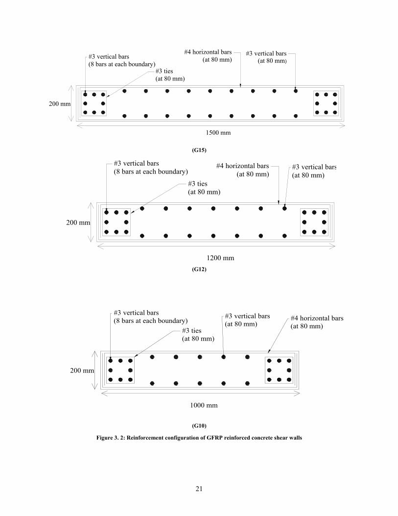
All specimens had web vertical and horizontal reinforcement consisting of two layers of #3 (9.5
mm) and #4 (12.8 mm) GFRP bars respectively. #3 (9.5 mm) vertical GFRP bars at web were
spaced at 120 mm, while #4 (12.8 mm) horizontal GFRP bars were spaced at 80 mm through the
height of the walls. Each wall had two boundary elements. Eight #3 (9.5 mm) GFRP bars were
used as vertical reinforcement in the boundaries. These vertical bars at boundaries were tied with
#3 (9.5 mm) rectangular GFRP spiral stirrups spaced at 80 mm. The reinforcement configuration
of the shear-wall specimens is shown in Fig. 3.2. Also, the reinforcement assembly of the shear
wall specimens on which Mohamed et al. (2013) conducted experiments at the University of
Sherbrooke is shown in Fig. 3.3, Fig. 3.4 and Fig. 3.5.
Axial loading
Lateral loading
h=3500 mm
W=1500 (G15); 1200 (G12); 1000 (G10)
t
21
(G15)
(G12)
(G10)
Figure 3. 2: Reinforcement configuration of GFRP reinforced concrete shear walls
#3 vertical bars
(8 bars at each boundary)#3 ties
(at 80 mm)
#4 horizontal bars
(at 80 mm)#3 vertical bars
(at 80 mm)
1500 mm
200 mm
#3 vertical bars
(8 bars at each boundary)
#3 ties
(at 80 mm)
#4 horizontal bars
(at 80 mm)#3 vertical bars
(at 80 mm)
200 mm
1200 mm
#3 vertical bars
(8 bars at each boundary)
#3 ties
(at 80 mm)
#4 horizontal bars
(at 80 mm)
#3 vertical bars
(at 80 mm)
200 mm
1000 mm

22
Figure 3. 3: Reinforcement cage of G10 (Mohamed et al. 2013)

23
Figure 3. 4: Reinforcement cage of G12 (Mohamed et al. 2013)

24
Figure 3. 5: Reinforcement cage of G15 (Mohamed et al. 2013)

25
Table 3.1 lists the reinforcement ratios. and b are the ratios of vertical reinforcement in the
web and boundaries respectively. h is the horizontal reinforcement ratio in the web of the walls.
t shows the ratio of the ties in the boundaries.
Table 3. 1: Reinforcement ratios of GFRP reinforced shear walls
Walls b h t
G15 0.58 1.43 1.58 0.89
G12 0.62 1.43 1.58 0.89
G10 0.59 1.43 1.58 0.89
3.2.2. Material Properties
All GFRP reinforcing bars used in the experiments were high-modulus sand-coated bars according
to the provisions of CSA S807 (CSA S807 2010). The properties of the GFRP bars are shown in
Table 3.2.
Table 3. 2: Material properties of reinforcement
Material ( )d mm 2( )A mm ( )E GPa ( )uf MPa (%)u
GFRP #3 9.5 71.3 66.9 1412 2.11
GFRP #4 12.8 126.7 69.6 1392 2

26
As for the concrete properties, the concrete used in the experiment was normal-weight and ready-
mixed. Its compressive strength ( 'cf ) and tensile strengths were 40 MPa and 3.5 MPa
respectively. Also, its ultimate concrete compression strain at extreme compression fiber ( cu ) as
recommended by the provisions in the CSA A23.3 (CSA A23.3 2004) code was taken as 0.0035.
The actual material properties of the concrete and reinforcement are shown in Fig. 3.6 (Mohamed
et al. 2014).
Figure 3. 6: Actual material properties of concrete and GFRP bars used in the experiment (Mohamed et al. 2014)
3.2.3. Loading
The horizontal load was applied to the shear walls in a displacement control mode. The typical
procedure for applying the quasi-static reversed cyclic loading is shown in Fig. 3.7. The loading
had two cycles at each displacement level. The first lateral displacement level was 2 mm. Then
two cycles were repeated in increments of 2 mm up to a lateral displacement level of 10 mm.
Afterward, displacements were applied with the increment of 5 mm up to the lateral displacement
of 50 mm. Then, displacements with the increment of 10 mm were applied to the walls up to the
failure.

27
Figure 3. 7: Displacement history
The total axial load applied to the walls was considered 0.07 ’cN wtf , in which w and t are
the width and thickness of the shear walls respectively. ’cf is the concrete compressive strength
in MPa. The axial stress was maintained constant throughout the duration of each test.
3.3. VecTor2 Modeling Process
The Modified Compression Field Theory (Vecchio and Collins 1986) and the Disturbed Stress
Field Model (Vecchio 2000) are the theoretical bases of VecTor2 for analyzing the nonlinear
behavior of the reinforced concrete membrane structures.
Several studies show that the Modified Compression Field Theory (MCFT) is an accurate
analytical model for predicting the load-deformation response, the concrete and reinforcement
strains and stresses, as well as the crack widths, orientation of cracks and the failure mode of
reinforced concrete membrane elements subjected to shear and normal stresses,
-150
-100
-50
0
50
100
150
0 10 20 30 40 50 60 70
To
p d
isp
lace
men
t (m
m )
Cycles

28
However, there are certain structures and special loading scenarios for which the MCFT cannot
predict the response (Wong et al. 2002). For example, the MCFT overestimates the shear stiffness
and strength of structures with lightly reinforced elements, where crack shear slip is significant.
This is because in lightly reinforced elements, the rotation of the principal stress field tends to lag
the greater rotation of the principal strain field, while the MCFT assumes the rotations are equal.
On the contrary, in elements that exhibit limited rotation of the principal stress and strain fields,
the MCFT generally underestimates the shear stiffness and strength. This is partly because the
concrete compression response calibrated for the MCFT is overly softened for the effect of
principal tensile strains.
VecTor2 describes the combined behavior of aggregates, cement and reinforcement through of
stress-strain relationships. The stiffness of the structure is determined from the stresses and strains
calculated from the constitutive and behavioral models. Therefore, the accuracy of the VecTor2
results depends on the constitutive models chosen for the analysis. The models and the elements
that are used in the modeling of the shear walls in this research are described in this section. More
detailed information on other elements or models is given in “VecTor2 & FormWorks User’s
Manual” by Wong et al. (2002).
The modeling of a structure in VecTor2 starts with the selection of models for material behavior
and loading conditions. VecTor2 predicts the response of reinforced concrete structures
considering the second-order effects such as compression softening, tension stiffening, tension
softening and tension splitting through some models. It also models the concrete expansion and
confinement, cyclic loading and hysteretic response, construction and loading chronology for
repair applications, bond slip, crack shear slip deformations, reinforcement dowel action,
reinforcement buckling, and crack allocation processes. The material models for concrete,
reinforcement and bond used for the shear walls modelled in this study are discussed in sections
3.3.1, 3.3.2 and 3.3.3 respectively.

29
After the material models have been selected, the elements for concrete, reinforcement and bond
regions are assigned. Reinforced concrete structures also require a relatively fine mesh to model
the reinforcement detailing and local crack patterns. Generating a mesh in VecTor2 is automatic.
Computational accuracy, computational efficiency and numerical stability are the advantages of
using low-powered elements and fine mesh in this software. The finite elements available in the
VecTor2 element library are discussed in section 3.3.4.
3.3.1. Models for Concrete
In this section, concrete constitutive and behavioral models are discussed. The pre-peak and post-
peak compression responses of the concrete were modeled based on the stress-strain model
proposed by Hoshikuma et al. (1997). The model used in this research for the hysteretic response
of the concrete was chosen according to the study conducted by Palermo et al. (2002). Also, the
slip distortion in the reinforced concrete was considered in the modeling of the shear walls
according to a model studied by Vecchio and Lai (2004). The tension stiffening of the concrete
was taken into the consideration by the model proposed by Bentz (2000). Confinement strength
was calculated using the model proposed by Kupfer et al. (1969). The Variable-Kupfer (Kupfer
and Gerstle 1973) and Mohr-coulomb (stress) are the models used for dilation and cracking
criterion modeling respectively.
3.3.2. Models for GFRP Reinforcement
The hysteretic response of the FRP reinforcement was modeled linearly. Based on the study
conducted by Deitz et al. (2003), the compressive modulus of elasticity for GFRP was equal to the
modulus of elasticity in tension ( gT gTE E E ). Also based on the same study, the compressive
strength of the FRP material ( guCf ) was taken as 50% of the ultimate tensile strength ( guTf ) as
shown in Fig. 3.8. According to the provisions of ACI 440 (ACI 440.1R 2006), the dowel action
was neglected for the GFRP reinforcement.

30
Figure 3.8: GFRP reinforcement hysteretic response
3.3.3. Models for Bond
The Eligehausen model (Eligehausen et al. 1983) was used for modeling the stress-slip
relationships of the bond between FRP bars and concrete in VecTor2. This model is shown in Fig.
3.9. It has an ascending non-linear branch, followed by a constant bond stress plateau and a linearly
declining branch. Subsequently, it has a sustaining residual stress branch.
Further details of all the above-mentioned models for concrete, reinforcement and bond stress-slip
relationship are available in the VecTor2 manual (Wong, Vecchio, and Trommels 2002).
fguT
1
E
fguC= 0.5* fguT
fguT
Stress
Strain

31
Figure 3. 9: Eligehausen bond stress-slip response
3.3.4. Element Library
There are various finite elements in the VecTore2 element library for modeling the concrete with
smeared reinforcement, discrete reinforcement and bond-slip mechanisms. Table 3.3 shows the
available elements in the VecTore2 element library (Wong, Vecchio, and Trommels 2002).
Table 3. 3: Elements in VecTor2 library
Material Elements
Plain Concrete or concrete with
smeared reinforcement
1. Three-node constant strain triangle
2. Four-node plane stress rectangular element
3. Four-node quadrilateral element
Bond- slip mechanism
1. Two-node link
2. Four-node contact element
Discrete reinforcement 1. Two-node truss-bar
τ
∆

32
Table 3.3 shows there are two options for modeling the reinforcement in concrete structures,
smeared reinforcement or discrete bars. Figure 3.10 shows two VecTor2 models with these two
types of reinforcement for G10. In both models, the horizontal reinforcement is modeled as
smeared reinforcement. However, the vertical and the diagonal reinforcement are modeled by
discrete reinforcement in Fig. 3.10 (a), and smeared one in Fig. 3.10 (b). Figure 3.11 shows the
load displacement diagram for these two models. Table 3.4 compares the values of ultimate load
capacity and maximum displacement of these walls. It shows that both models predict the ultimate
load approximately the same with a difference of 0.2 percent. Also, there is a difference of 1.5
percent for in the maximum displacement which is assumed to be negligible. Therefore, based on
the geometry and the reinforcement configuration, each option of reinforcement modeling is
equivalent to each other.
Table 3. 4: Comparison of the different types of reinforcement modeling (G10 wall)
Type of reinforcement Discrete reinforcement Smeared reinforcement Difference (%)
Ultimate Load (kN) 326.1 325.4 0.2
Maximum displacement (mm) 125.9 123.9 1.5

33
(a) (b)
Figure 3. 10: VecTor2 modeling for G10; (a) discrete reinforcement; (b) smeared reinforcement

34
Figure 3. 11: Load displacement response of G10 with two types of reinforcement modeling
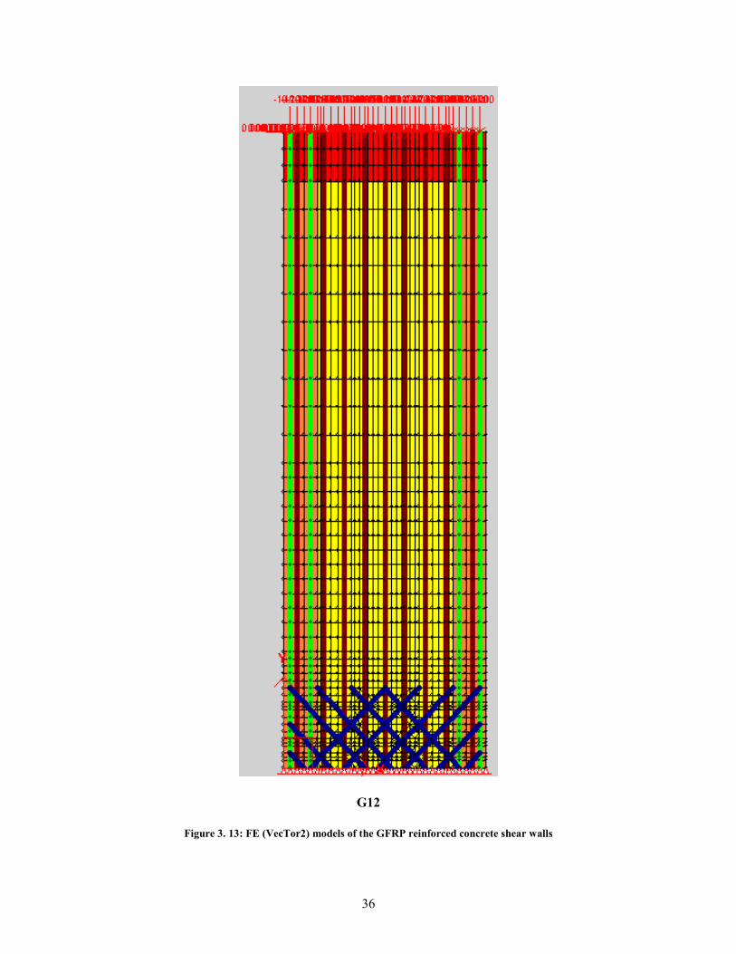
To validate the model, shear walls were modeled using a combination of smeared and vertical
reinforcement. For the longitudinal and diagonal GFRP reinforcing bars, two-node truss bar
elements are used, while the horizontal reinforcement for all specimens is modeled as smeared.
Different concrete material types are utilized for the regions with different ratios of horizontal
reinforcements. The VecTor2 models for G10, G12 and G15 are shown in Fig. 3.12, Fig. 3.13 and
Fig. 3.14 respectively.
0
50
100
150
200
250
300
350
400
0 20 40 60 80 100 120 140
Lo
ad
(K
N)
Displacement(mm)
G10
Smeared Reinforcmenet
Discrete reinforcement

35
G10
Figure 3. 12: FE (VecTor2) models of the GFRP reinforced concrete shear walls
36
G12
Figure 3. 13: FE (VecTor2) models of the GFRP reinforced concrete shear walls

37
G15
Figure 3. 14: FE (VecTor2) models of the GFRP reinforced concrete shear walls

38
Nodes at the bottom of the walls were restrained from displacements in the horizontal and vertical
directions. For modeling the loading in VecTor2, one load case was utilized to impose the
horizontal displacement at the top of the wall. The load factor was increased cyclically from zero
to failure in the increments described in section 3.2.3. The vertical load is distributed as
concentrated forces in the y-direction on individual nodes at the top of the wall. The self-weight
of the walls is not considered as it is negligible in comparison to the applied vertical load.
As for the meshing options, the automatic mesh generation facility with the hybrid discretization
type was used to create the mesh in VecTor2 models. To formulate a suitable finite-element mesh
for shear walls, at first, the number of distinct modeling zones in the shear walls was determined
bases on the changes in geometry, material properties and reinforcement ratio and configuration.
For the GFRP reinforced shear walls in this research, the concrete strength is uniform; however,
changes in the quantity and the configuration of reinforcement, both smeared and discrete,
necessitated modeling of multiple zones. After establishing the zones, a suitable finite-element
mesh for capturing the features of the structural behavior of the shear walls must be developed.
According to the study conducted by Palermo and Vecchio (2007) when prior knowledge of
structures behavior is unknown, the elements sizes are acceptable when the global displacements
and local stresses remain unchanged (or the changes are within the tolerances required for the
design) if the number of elements is doubled. On the other hand, if the prior knowledge of the
reinforced concrete structure is available from the experimental results, continual refinement of
the mesh (decreasing the element size) can be done until analytical and experimental results reach
an acceptable agreement. In this research, since the experimental results were available, the later
method was used for choosing the acceptable mesh size. The typical finite element mesh for the
GFRP reinforced shear walls is shown in Fig. 3.15. The element sizes were chosen for each wall
provided a relatively fine mesh and led to a close agreement with the test results. In addition, no
further improvement of the response was obtained when the number of elements increased by a
factor of 2.

39
Figure 3. 15: Typical finite element mesh (G10)
40
3.4. Analytical Analysis Results (VecTor2)
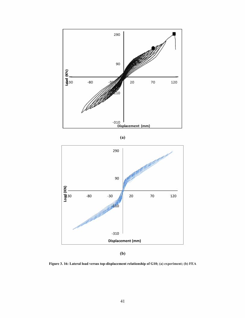
The experimental results and the analytical responses of the shear walls are shown in Fig. 3.16,
Fig. 3.17 and Fig. 3.18 for G10, G12 and G15 respectively.
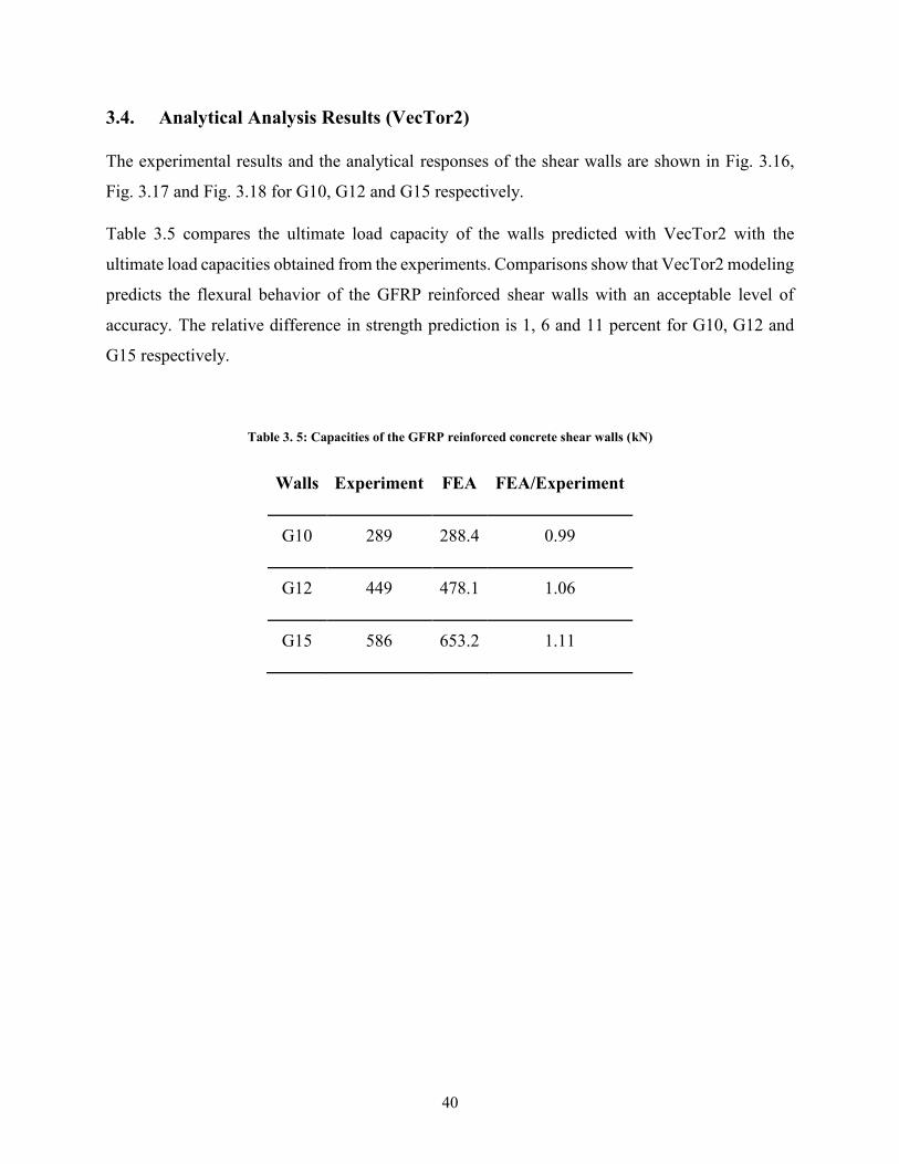
Table 3.5 compares the ultimate load capacity of the walls predicted with VecTor2 with the
ultimate load capacities obtained from the experiments. Comparisons show that VecTor2 modeling
predicts the flexural behavior of the GFRP reinforced shear walls with an acceptable level of
accuracy. The relative difference in strength prediction is 1, 6 and 11 percent for G10, G12 and
G15 respectively.
Table 3. 5: Capacities of the GFRP reinforced concrete shear walls (kN)
Walls Experiment FEA FEA/Experiment
G10 289 288.4 0.99
G12 449 478.1 1.06
G15 586 653.2 1.11
41
(a)
(b)
Figure 3. 16: Lateral load versus top-displacement relationship of G10; (a) experiment; (b) FEA
-310
-110
90
290
-130 -80 -30 20 70 120
Load
(K
N)
Displacement (mm)

42
(a)
(b)
Figure 3. 17: Lateral load versus top-displacement relationship of G12; (a) experiment; (b) FEA
-500
-300
-100
100
300
500
-130 -80 -30 20 70 120
Load
(K
N)
Displacement (mm)

43
(a)
(b)
Figure 3. 18: Lateral load versus top-displacement relationship of G15; (a) experiment; (b) FEA
-630
-430
-230
-30
170
370
570
-130 -80 -30 20 70 120
Load
(K
N)
Displacement (mm)

44
The analysis shows that VecTor2 models can predict the failure mode of the shear walls. The
shear walls met the minimum longitudinal reinforcement requirements determined by the code and
design guide provisions (ACI 440.1R 2006; CSA S806 2012). Therefore, all three walls failures
were designed to fail by concrete crushing, which is the desirable mode of failure for FRP
reinforced members. Figure 3.19 shows that VecTor2 can predict the failure mode of the shear
walls accurately. At the failure point, the concrete compressive stress reached its peak strength 40
MPa, while the stresses in GFRP bars were lower than their ultimate strength.
Figure 3. 19: Concrete crushing mode of failure for G15
Concrete crushing

45
The results also show that VecTor2 can predict the cracked state of the shear walls with reasonable
accuracy. The comparison between the crack pattern of one of the specimens, G15, is shown in
Fig.3.20.
(a) (b)
Figure 3. 20: Typical crack pattern of GFRP reinforced concrete shear walls; (a) FEA; (b) experiment

46
4. Chapter 4. Economic Design of FRP-Reinforced RC Shear Walls
A technique to conduct the economic design of concrete shear walls reinforced with FRP bars is
discussed in this chapter. The process consists of analyzing the structural response of a series of
FRP-reinforced walls in terms of strength, deflection, cracking, among other constraints of interest,
and compare it to that of a reference wall, made with conventional steel-reinforced concrete. When
plotted in a diagram of width vs. reinforcement ratio, the strategy allows the identification of
feasible regions in which FRP-reinforced walls have comparable (or superior) performance
compared to steel-reinforced walls. The procedure is illustrated via a design example.
4.1. Background
As discussed earlier, even though FRP bars in reinforced concrete structures have shown superior
properties such as high strength and high resistance to corrosion in comparison to conventional
steel reinforcement, their market share remains small. This is attributed to several factors: a
perceived high cost, uncertainties about long-term performance, and the different design principles
used when compared to designs using conventional steel rebar (Balafas and Burgoyne 2012). One
way to illustrate the feasibility of using FRP reinforcement is to demonstrate the ranges in common
design variables in which FRP can be used at a minimum cost while having comparable
performance to steel-reinforced concrete structures.
4.2. Width/Depth vs. Reinforcement Ratio Diagram
A beam depth vs. flexural reinforcement area diagram was used by Al-Salloum and Husainsiddiqi
(1994) to determine the most economical design of the singly steel reinforced rectangular beams
based on the provisions in ACI 318 (ACI 318M 1989). Balafas and Burgoyne (2012) used a similar
tool to investigate the feasibility of using FRP reinforcement in beams using the same diagram,
considering additional design constraints, specific to FRP materials.
To illustrate how the process can be used to determine the optimal design options for FRP-
reinforced walls, several shear walls with various concrete dimensions and FRP reinforcement

47
ratios are considered, and their structural response is compared to a reference control wall
reinforced with steel rebars for a building to be designed in Edmonton.
Applying the techniques developed by Al-Salloum and Hussainsiddiqi (1994) and Balafas and
Burgoyne (Balafas and Burgoyne 2012) to FRP-reinforced shear walls, a feasible design region on
a diagram of shear wall width against flexural bar reinforcement ratio ( w ) can be determined
for the tested walls. In this diagram, reinforcement ratio is the ratio of the flexural reinforcement
area to the cross section area of the shear wall. In the feasible design region, FRP-reinforced walls
have comparable (or superior) performance compared to steel-reinforced walls with regards to
different design constraints.
4.3. Example Shear Wall Building
A nine-storey reinforced concrete office building in Edmonton has 6 bays of 7.5 m in the E W
direction and 3 bays of 6.5 m in the perpendicular direction ( N S ). The typical story height ( sh )
is 3 m. The total height of the building ( h ) is 27 meters. The plan and the elevation views for this
building are shown in Fig. 4.1.
The structural wall, 1 bc , in the plan view, Fig. 4.1 (a), shows the location of the shear walls
studied in this research. The exterior shear walls were chosen in this study because they are more
vulnerable to corrosion compared to the internal shear walls which are not exposed to the harsh
environmental conditions outside the building.
All the wall specimens were 27000 mm in height h , and 200 mm in thickness ( )t . The wall
lengths w were various ranging from 4500 mm to 13500 mm resulting in a shear wall aspect ratio
/h w of 2 to 6 which classifies them as slender walls. They have rectangular cross-sections with
no flanges. These designs against lateral loads are assumed to be controlled by wind forces.
The shear walls studied in this research are walls with simple, rectangular cross-sections, and are
designed for non-seismic conditions. The walls are designed to resist lateral loads acting parallel
to the plane of the wall, and axial loads occur within the plane of the wall, but act along the vertical
axis of the wall.. Generally, the vertical loads can be downward-acting gravity loads that result

48
from the weight of the structure or upward-acting (uplift) loads from wind or seismic events. Axial
loads (vertical loads) are transferred into the shear walls from the roof (or upper story walls) above.
In this study, the gravity load, N, acting on the walls is considered equal to seven percent of the
section capacity (Eq. 4.1) which is a value commonly found in practice for walls in low- to mid-
rise RC buildings (Mohamed et al., 2013). In Eq. 4.1, w is the width of the wall, t is the wall
thickness, and ’cf is the 28-day peak compressive strength of the concrete. The building is
assumed to behave in a flexural manner, with structural walls assumed to act as vertical cantilevers
to resist the lateral load – the maximum moment appears at the base.
0.07 cN w t f (4. 1)
(a)
c
b
1 2 3 4 5 6 7
N
d
a
w

49
(b)
(b)
Figure 4. 1: Shear wall building; (a) plan view; (b) elevation view
The shear walls used in this research were designed under the assumption that they fall in the
conventional construction classification of resisting systems in the National Building Code of
Canada (NBCC 2015 ). These are used mostly for non-seismic regions. The reinforcement in the
walls is designed to preclude sliding and shear failures, thus promoting a flexural ductile failure.
The point of the investigation is to determine the dimensions and flexural reinforcement of FRP-
reinforced walls that can replace the steel-reinforced walls to achieve comparable (or superior)
performance in terms of strength, deflections, cracking and other constraints. Evidently, the
optimal solution should also lead to minimal geometry changes so that the FRP-walls can be
included in the design with minor variations.
Later, same shear walls with the same wall dimensions and reinforcement ratios but with steel
reinforcement were modeled for comparison.
The FRP material chosen in this case study was GFRP. Material properties for the steel and GFRP
materials used in the walls are shown in Table 4.1.
w
h=27 m

50
Table 4. 1: Material properties of reinforcement
Material ( )E GPa ( )yf MPa ( )uf MPa (%)y (%)u
GFRP 66.9 - 1412 - 2.11
Steel 200 400 550 0.2 -
Figure 4.2 shows the schematic wall dimensions and the reinforcement details of the shear walls
with both types of reinforcements, GFRP and steel.
Figure 4.2: Concrete dimensions and reinforcement configuration of the shear walls
The thickness of the walls was kept constant. All the walls were 200 mm thick. There is a minimum
thickness ( mint ) for shear walls reinforced with steel bars according to the provisions in CSA
A23.3 (CSA A23.3 2004) and ACI 318 (ACI 318M 2008) to avoid excessively thin walls that
27000 mm
w
t w= 4500 to 13500 mm
t=200 mm
Vertical reinforcement (ρ)
Horizontal reinforcement

51
would buckle out-of-plane. According to these provisions, the thickness of the walls should not be
less than 25
sh where sh is the unsupported height of the wall. The unsupported height of the walls
in the building is the story height, sh , which is 3 meters. Therefore, the minimum thickness ( mint )
of the wall can be obtained from Eq. 4.2. The same minimum thickness is specified by ACI 440
(ACI 440.1R 2006) and CSA S806 (CSA S806 2012) design guides for FRP-reinforced shear
walls.
min
3000120
25 25
sht mm (4.2)
Therefore, the fixed thickness of 200 mm meets the minimum thickness requirements determined
by the code provisions.
4.4. Reference Wall
One steel reinforced shear wall in the building was designed to comply with the
requirements specified in CSA A23.3 (CSA A23.3 2004) and ACI 318 (ACI 318M
2008) and used as a reference wall. Figure 4.3 shows the schematic cross section
dimensions and the reinforcement details of the reference shear wall. The reference
wall has the same location in the building as other GFRP reinforced concrete shear
walls, 1 bc in the plan view (Fig. 4.1 (a)).
Figure 4.3 shows the concrete dimensions and reinforcement ratios for the reference
wall in this study. The height and the thickness of the reference wall is 27000 mm and
200 mm, respectively. The width is equal to 6750 mm.
For the reference wall in this research, the vertical and horizontal reinforcement ratios
were chosen as 1.0 and 1.5 percent of the cross-section area respectively. Since the
objective of this study is not to investigate the design of conventional RC walls for a
set of given loads in a region, but the comparative design between FRP- and steel-
reinforced walls, these reinforcement ratios were chosen arbitrarily. However, based on
a survey conducted among structural engineers, these ratios are typical of zones with
high-wind pressures.

52
For the reference wall and all other steel reinforced walls investigated in section 5.1,
the minimum areas of the vertical and the horizontal reinforcement are 0.0015 gA and
0.002 gA respectively according to the provisions in CSA A23.3 (CSA A23.3 2004).
Thus, the chosen ratios comply with the minimum reinforcement requirement.
The load corresponding to the service condition was determined in terms of allowable
stresses in the concrete and the steel, and in terms of deflections. The concrete
compressive stress under service loads was limited to 40% of 'cf . For steel, the
maximum tensile stress in the bars was limited to 60% of yf . The governing
maximum deflection under service loads was 1/500 of the height the building. The
service load was determined as 546 kN. Additional details for the service load
calculation are given in Section 4.5.3.
Figure 4.3: Cross section of the reference shear wall reinforced with steel bars
The ultimate load capacity of the reference wall, termed as reference ultimate strength,
was calculated as 1112 kN based on pushover analysis of the reference shear wall
conducted with finite-element program Vector2, which agreed closely with a plane-
section compatibility analysis of the cross-section. That was to be expected since the
wall is a slender element in which Bernoully theory holds well. The Vector2 model and
the pushover response of the reference shear wall are shown in Fig. 4.4.
As shown in Fig. 4.4, in the modeling of the reference wall and also other shear walls
under study in this research, the lateral and the axial load are applied at the top of the
6750 mm
200 mm
ρ=1%
Ρh=1.5%

53
shear walls, while the actual loads are applied at each floor. This assumption is made
for modeling simplification and has negligible effect on the analytical results of the
shear walls performances.
(a)
Lateral loading
Axial
loading

54
(b)
Figure 4.4: Reference wall; (a) VecTor2 model; (b) load-displacement response
4.5. Design Constraints
4.5.1. Ultimate Strength
To find the strength constraint, the pushover analysis for a number of walls having the same height,
but varying widths and vertical reinforcement ratios was conducted in Vector2. Then, their
ultimate strengths were compared to the ultimate strength of the reference wall. The ultimate
strength was defined as the point in which the load-displacement response drops more than 20%
regarding the peak load.
For example, the pushover responses of two GFRP reinforced shear walls are shown in
Fig. 4.5. These two walls have the same width, 6750 mm, height, 27000 mm, and thicknesses, 200
mm. The horizontal reinforcement ratio is the same for both equal to 1.5%. However, the vertical
reinforcement ratios are 0.25% and 0.75%. Comparing their ultimate strength with the reference
ultimate strength of 1112 MPa, the one with 0.25% GFRP reinforcement has lower ultimate
strength than that of the reference wall – this wall would be inadequate to be used in the building,
Ultimate
strength=1112(KN)
0
200
400
600
800
1000
1200
0 200 400 600 800 1000
Lo
ad
(K
N)
Displacement(mm)
Reference wall response

55
because it is assumed that the load demand is independent from the material used to build the
walls. In comparison, the wall with 0.75% GFRP reinforcement is stronger than the reference wall
; thus, it is an acceptable alternative (Fig. 4.5).
Repeating the same procedure for other GFRP reinforced shear walls, the ultimate strengths of
the walls are shown in Fig. 4.6. Only some values are shown for clarity. The walls which are
stronger than, or as strong as, the reference wall are shown with cross markers, while those which
are not strong enough are shown with circular markers. The numbers next to the markers represent
the calculated ultimate strength.
Figure 4.5: Push-over response of GFRP reinforced shear walls
0
200
400
600
800
1000
1200
1400
1600
0 200 400 600 800 1000
Lo
ad
(K
N)
Displacement(mm)
Reference wall
ρ=0.25%, w=6750 mm
ρ=0.75%, w=6750 mm
824 kN
1112 kN
1436 kN

56
Figure 4.6: Ultimate strengths of the shear walls
Considering the values in Fig. 4.6, for each wall aspect ratio, there is a minimum reinforcement
ratio that enables the wall to reach the reference ultimate strength. These minimum reinforcement
ratios create a strength constraint curve in the width against GFRP reinforcement ratio diagram
(Fig. 4.7). The walls which are as strong as the reference wall lie on the constraint line. Walls that
are stronger lie above the constraint, while those that are not sufficiently strong lie in the
inadequate region below the line. Figure 4.7 (b) shows how the strength constraint curve divides
the w-ρ diagram into two feasible and infeasible regions.
376535
825
1292
3851
515737
1142
2075
4674
639922
1436
2618
5888
7451101
1676
3103
7629
8551245
1940
3505
8050
9401352
2193
3938
8365
0
1500
3000
4500
6000
7500
9000
10500
12000
13500
0 0.2 0.4 0.6 0.8 1 1.2 1.4 1.6
Wid
th (
mm
)
FRP - vertical reinforcement ratio (%)

57
(a)
(b)
Figure 4.7: (a) separating line; (b) strength constraint
Strength
constraint
0
1500
3000
4500
6000
7500
9000
10500
12000
13500
0 0.2 0.4 0.6 0.8 1 1.2 1.4 1.6
Wid
th (
mm
)
FRP - vertical reinforcement ratio (%)
Feasible zone

58
4.5.2. Bar Fracture
The flexural design philosophies used for the steel and FRP reinforced concrete elements have
significant differences. In flexural members reinforced with steel bars, yielding of steel before
crushing of concrete is desired. Yielding of the steel provides ductility and a warning of failure
(ACI 440.1R 2006). Since there is no yielding or equivalent concept for FRP materials, codes
provide explicit provisions requiring that failure must be controlled by concrete crushing in
compression rather than reinforcement fracture in tension (Nanni 1993). If FRP bars rupture, there
would be only a limited warning of failure due to the small elongation that FRP reinforcement
experiences before rupture.
A general comparison between testing data in steel- and FRP-reinforced shear walls shows that in
both cases of failure of FRP-reinforced members, either bar fracture or concrete crushing, FRP
reinforced members do not exhibit ductility as is commonly observed in under-reinforced,
conventional concrete shear walls reinforced with steel rebars (ACI 440.1R 2006).
The above discussion leads to the conclusion that a FRP fracture constraint should be included
into the width against reinforcement ratio diagram. This would enable designers to identify at a
glance which walls exhibit rupture of the bars before crushing of the concrete.
For each wall with specific aspect ratio, there is a minimum reinforcement ratio that ensures
concrete crushing as the mode of failure. This ratio is called the balanced reinforcement ratio, b
, which is the ratio in the section where concrete crushing and FRP rupture occur simultaneously.
If the reinforcement ratio is less than the balanced ratio ( b ), FRP rupture is the mode of
failure. Otherwise, if b , concrete crushing governs, which is desirable.
Figure 4.8 shows concrete crushing, bar fracture and the balanced modes of failure for FRP
reinforced shear walls in terms of plane-section compatibility analyses. For the first section, Fig.
4.8 (a), illustrates the concrete crushing mode of failure. The maximum unconfined concrete strain
at the extreme compression fiber ( cu ) as recommended by the provisions in CSA A23.3 ((CSA
A23.3 2004) to be taken as 0.0035. However, in the bar fracture mode of failure, Fig. 4.8 (b), the
strain in the concrete is less than the its ultimate strain, with the tensile FRP reinforcement reaching
its ultimate design strain. The rupture strain of the FRP bars used in this research is 0.021 (typical
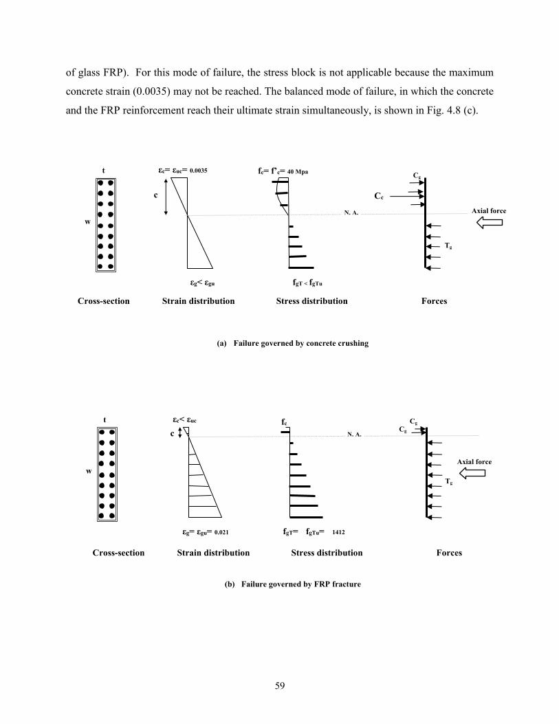
59
of glass FRP). For this mode of failure, the stress block is not applicable because the maximum
concrete strain (0.0035) may not be reached. The balanced mode of failure, in which the concrete
and the FRP reinforcement reach their ultimate strain simultaneously, is shown in Fig. 4.8 (c).
(a) Failure governed by concrete crushing
(b) Failure governed by FRP fracture
fc= f’c= 40 Mpa
fgT < fgTu
t
w
εc= εuc= 0.0035 c 0.
00
35
εg< εgu
N. A. Cc
Cg
Tg
Axial force
Cross-section Strain distribution Stress distribution Forces
fc
fgT= fgTu= 1412
MPa
t
w
εc< εuc c 0.
00
35
εg= εgu= 0.021
N. A. Cg
Cg
Tg
Axial force
Cross-section Strain distribution Stress distribution Forces

60
(c)Balanced failure condition
Figure 4.8: Strain and stress distribution at ultimate conditions
The sections with the balanced reinforcement ratio can be shown with a line in the w diagram
termed “balanced-section” constraint. The balanced section line is shown in Fig. 4.9. Shear walls
with less reinforcement ratio than the balanced reinforcement ratio lie at the left-hand side of the
line. These walls fail by bar fracture, an undesirable failure mechanism. Sections with
reinforcement ratios higher than the balanced reinforcement lie at the right-hand side of the
balanced line. These exhibit a desirable concrete crushing mode of failure.
A simplified plane-sectional analysis can be conducted to illustrate why the balanced line is
vertical, as shown in Fig. 4.9.
That is, for the types of wall under study, the balanced reinforcement percentage is independent of
the wall width. The plan sectional analysis is based on the strain compatibility, internal force
equilibrium, and the use of simplified constitutive relationships.
fc= f’c= 40 Mpa
fgT= fgTu= 1412
MPa
t
w
εc= εuc= 0.0035 c 0.
00
35
εg= εgu= 0.021
N. A. Cc
Cg
Tg
Axial force
Cross-section Strain distribution Stress distribution Forces

61
Figure 4.9: Balanced sections line
CSA A23.3 (CSA A23.3 2004) defines an equivalent rectangular stress block to represent the
parabolic distribution of compression stresses in the concrete. The rectangular stress distribution
spreads over a depth and a width of 1a c and 1 ’cf respectively. The balanced reinforcement
is determined from equilibrium of internal and external forces shown in Fig. 4.8 (c). This
equilibrium condition is expressed in Eq. 4.3.
c g gC C T N (4.3)
Because FRP does not yield, the forces in the FRP reinforcement are computed in Eq. 4.4 using
its design tensile and compressive strengths ( gTf and gCf ). Throughout the calculations, the
reduction factors are considered to be equal to 1.
1 1'c gC gC gT gTf ct A f A f N (4.4)
Strength
constraint
0
1500
3000
4500
6000
7500
9000
10500
12000
13500
0 0.2 0.4 0.6 0.8 1 1.2 1.4 1.6
Wid
th (
mm
)
FRP - vertical reinforcement ratio (%)
Feasible zone
Balanced
sections
Concrete crushing
Bar
fracture

62
The parameters 1 and 1 determine the dimensions of an equivalent stress block for the concrete
in ultimate condition, and can be obtained from the following equations (Eq. 4.5 and Eq. 4.6)
1 0.85 0.0015 ' 0.79 0.67cf (4.5)
1 0.97 0.0025 ' 0.87 0.67cf (4.6)
While N is the axial load of 0.07 ’cwtf (Eq. 4.1) applied at the top of the walls, and c is the depth
of the neutral axis, which can be expressed as a proportion of the wall width w as shown in Eq.
4.7. This equation is written using similar triangles as shown in the strain distribution diagram in
Fig. 4.8 (c), assuming an ultimate strain in the FRP material of 0.021.
0.00350.0143
0.021
cc w
w c
(4.7)
This way, all the components of the Eq. 4.4 can be written in terms of both w and t variables as
shown in Eq. 4.8. Therefore, these variables, w and t , can be canceled out from all the
components in two sides of this equation. This makes the balanced flexural reinforcement ratio
( ) independent of the cross-section dimensions, w and t .
1 1' (0.0143 ) 0.07 'c gC gC gT gT cf w t wtf wtf f wt (4.8)
Equation 4.9 shows the new form of Eq. 4.8 considering the above-mentioned definitions.
1 10.0143 ' 0.07 'c gC gC gT gT cf f f f (4.9)
The area of the compression and tensile reinforcement, gCA and gTA , can be expressed in terms
of reinforcement ratios as gCwt and gT wt respectively ( gC gT ). The tensile and
compressive layers of reinforcement can be determined by the location of the neutral axis using
similar triangles. Since the reinforcement is distributed evenly in the cross section, gC and gT
can be determined according to the location of the neutral axis as shown in the following equations
(Eq. 4.10 and Eq. 4.11).

63
0.0143
0.0143gC
c w
w w (4.10)
0.01430.9857gT
w c w w
w w
(4.11)
The stresses in each layer of FRP in compression gCf and tension gTf , can therefore be obtained
from Eq. 4.12 and Eq. 4.12.
gT gTf E (4.12)
gC gCf E (4.13)
Where E is the modulus of elasticity, and is the strains in reinforcement. Based on the study
conducted by Deitz et al. (2003), the compressive modulus of elasticity for GFRP is equal to the
modulus of elasticity in tension ( gT gTE E E ). Deitz et al. (2003) also suggests that the
compressive strength of the FRP material be taken as 50% of the ultimate tensile strength.
Equation 4.14 shows the new form of Eq. 4.9 substituting the values of gC , gT , gCf and gTf
into the Eq. 4.9.
1 10.0143 ' 0.0143 0.9857 0.07 'c gC gT cf E E f (4.14)
The balanced reinforcement ratio ( b ) can be obtained from solving Eq. 4.14 for . In this study
is equal 0.0025.
VecTor2 enables the analyst to determine the failure modes by calculating the stresses in the
materials at failure. A visual representation of concrete crushing and bar fracture failure modes is
presented in Fig. 4.10. The results from Vector2 were in good agreement with the hand-calculation
given in Eq. 4.14.

64
Figure 4.10: Failure modes of the FRP reinforced concrete shear walls
Concrete crushing
Bar Fracture
Lateral load
Lateral load

65
Serviceability
Serviceability of RC elements can be characterized in terms of different response parameters. The
focus of this investigation is on the deflection and cracking service limit states, but others can be
studied in a similar manner.
Deflections and crack width should be within the acceptable limits specified by code provisions.
The reinforcement type has a significant impact on the magnitude of deflection and cracking. For
instance, FRP bars lead to larger deflections and wider crack widths compared to those occurring
when steel reinforcement is used (Masmoudi et al. 1996; Tighiouart et al. 1998).
4.5.3. Deflection at Service Condition
In general, code provisions for deflection control address deflections that occur at service levels
under immediate and sustained static loads. In FRP-reinforced shear walls, the low modulus of
elasticity of the reinforcement has the potential to lead to large deflections. Therefore, FRP
reinforced concrete members should be designed to have adequate stiffness to limit deflections
that may adversely affect their serviceability.
In a survey of leading building codes, Griffis (2003) found that the limit for the inter-story drift
ratios for wind load ranged between 200
sh to
600
sh, with the most widely values being reported as
400
shto
500
sh, depending on the building type and the construction materials. The parameter sh ,
inter story height, is the height from grade to the uppermost floor.
In this research, the total drift per storey under service wind and gravity load has been assumed to
be 1
500of the building height, / 500h , which is the same as the limit proposed by the National
Building Code of Canada (NBCC 2015 ). The NBCC 2015 limit is applicable for all type of
buildings except for industrial buildings and sheds in which greater movement will have no
significant adverse effects on the strength and the function of the building. The magnitude of the
wind load is usually the same as that used in proportioning the frame for strength, and typically is
based on a 50-year or 100-year mean recurrence interval load for normal buildings and critical
structures respectively (Griffis 2003).

66
To apply the deflection constraint into the width against reinforcement ratio diagram, the working
load (WL ) of the reference wall in the service condition is required. The service condition for the
reference wall is determined considering the service strength of concrete and the reinforcement.
The minimum deflection related to these two stresses is the service deflection for the reinforced
concrete shear wall. The concrete compression stress under service loads is limited to 40% of the
characteristic concrete strength (40 MPa in this study). The deflection related to this stress is called
1 . The maximum stress in the steel bars under loads at serviceability limit state was set at 60%
of the characteristic yield strength (400 MPa in this study). The displacement related to this
strength is 2 . The load corresponds to the minimum of these two displacements, 1 and 2 , is
called the working load. Figure 4.11 shows the load-displacement curve of the reference wall. The
values corresponding to 1 and 2 , and their minimum are shown in the following equations.
Regardless of the value of 1 and 2 , they should not exceed 54 mm
( / 500 27000 / 500 54hs ).
1 ( 16 ) 25fc MPa mm (4.15)
2 ( 240 ) 51fs MPa mm (4.16)
1 2( , ) 25Service Min mm (4.17)
The working load at the minimum displacement, 25mm, can be obtained from the load-
displacement response as:
( ) 546.4ServiceServicef f KN (4.18)

67
Figure 4.11: Service displacement and working load of the reference wall
For FRP reinforced walls, service stresses in the FRP material should be kept below acceptable
limits. The ACI 440 code recommends that the maximum stress in FRP materials at the
serviceability limit state be taken equal to equal to 25% of its characteristic tensile strength,
0.25* 0.25*1412 353gTuf MPa .
To apply the deflection constraint into the width against reinforcement ratio diagram, pushover
analyses were conducted for all the walls, and the load-displacement curves were obtained. The
deflection constraint depends on two conditions.
First, the deflection of the FFRP wall at the working load should be less than the maximum
allowable service displacement determined as per NBCC (2015), which is equal to 54500
hmm .
Second, the stresses in the materials of the walls (concrete and FRP) should be less than their
allowable limits under a lateral load equal the working load determined for the reference wall. This
Working load
=546.4(KN)
0
200
400
600
800
1000
1200
0 200 400 600 800 1000
Lo
ad
(K
N)
Displacement(mm)
Reference wallReference wall
fs=240MPa
fc=16 Mpa
∆1 ∆2

68
is because it is assumed that the service loads are independent from the material from which the
walls are made.
All the walls in which both conditions are satisfied simultaneously are categorized as the
acceptable walls in terms of service conditions for the deflection constraint.
Conducting the analysis in Vector2 for a number of walls (Fig. 4.12), a line in the width against
reinforcement ratio diagram can be drawn that divides the walls into two groups of acceptable and
unacceptable walls in terms of service deflection constraint as shown in Fig. 4.13.
Figure 4.12: Acceptable () and unacceptable (.) shear walls in terms of service deflection criteria
0
1500
3000
4500
6000
7500
9000
10500
12000
13500
0 0.2 0.4 0.6 0.8 1 1.2 1.4 1.6
Wid
th (
mm
)
FRP - vertical reinforcement ratio (%)

69
(a)
(b)
Figure 4.13: (a) separating line; (b) deflection constraint
Feasible zone
Strength
constraint
0
1500
3000
4500
6000
7500
9000
10500
12000
13500
0 0.2 0.4 0.6 0.8 1 1.2 1.4 1.6
Wid
th (
mm
)
FRP - vertical reinforcement ratio (%)
Balanced
Deflection constraint
Feasible zone

70
4.5.4. Crack Width at Service Condition
Corrosion and unsightly appearance are two reasons for limiting the crack width in reinforced
concrete structures.
Crack width limits in the concrete codes have the purpose of reducing the exposure of the
reinforcement to the moisture or other substances in aggressive environments. Corrosion can lead
to a rapid and significant deterioration of concrete structures (Kassem, Ahmed, and Benmokrane
2011).
For steel-reinforced structures, the provisions in both CSA A23.3 (CSA A23.3 2004) and ACI 318
(ACI 318M 2008) provide consistent crack width provisions that correspond to a maximum crack
width of 0.3 mm for exterior exposure and 0.4 mm for interior exposure.
The crack widths in FRP-reinforced members are expected to be larger than those in steel-
reinforced members under similar loads, due to the lower modulus of elasticity of FRP material in
comparison to that of steel. This is because a lower modulus of elasticity leads to larger deflections
and therefore wider cracks. However, the maximum crack width limitation can be relaxed for the
FRP-reinforced structures in comparison to the conventional steel-reinforced structures, because
FRP does not corrode. This is recognized in the provisions of CSA S806 (CSA S806 2012)
allowing crack widths of 0.5 mm and 0.7 mm for exterior and interior exposure, respectively.
In general, according to the studies conducted by Mias et al. (2015), Kassem et al. (2011) and
Michèle Thériault and Benmokrane (1998), the crack widths in flexural members decrease as the
reinforcement ratio increases.
Equation 4.19, which appears in the provisions of both ACI 440 and CSA S806 indicates that the
crack depends largely on the spacing and distribution of the bars.
2 22 ( )2
f
c b c
f
f sw k d
E (4.19)
Where:
cw = maximum crack width, mm
ff = stress in FRP reinforcement in tension, MPa

71
fE = modulus of elasticity of FRP bar, MPa
= ratio of distance from neutral axis to extreme tension fiber to distance from neutral axis to
centroid of reinforcement
bk = bond-dependent coefficient
cd = thickness of concrete cover measured from extreme tension fiber to center of bar, mm
s = longitudinal FRP bar spacing, mm
ff , fE , cd and s are constant for all the walls. for the walls with smeared reinforcement is
almost equal to 1. The bk term is a coefficient equal to 1 for FRP bars having a bond behavior
similar to steel bars (CSA S806 2012).
To apply the crack width constraint into the width against reinforcement ratio diagram, A number
of FRP-reinforced walls with varying combinations of width and flexural reinforcement ratio were
analyzed using VecTor2 under lateral load. The crack width was investigated at the working load
level determined for the reference wall. Then, the maximum crack width of each wall is recorded.
If the crack width is less or equal than the allowable limit of 0.5 mm (assuming exterior exposure),
the walls is said to be in the feasible zone. Otherwise, it deemed to have failed the crack width
criteria at service conditions.
For example, a GFRP reinforced shear wall is considered. The height, width and the vertical
reinforcement ratio are 27000 mm, 9000 mm, and 0.5 percent respectively. The load-displacement
response of the wall is shown in Fig. 4.14. The displacements related to the service conditions of
the concrete and the reinforcement are shown in this figure as well. These displacements are shown
in Eq. 4.20 and Eq. 4.21 respectively. The minimum of these two values which is the service
displacements calculated in Eq. 4.22.
1 ( 16 ) 19fc MPa mm (4. 20)
2 ( 353 ) 100fg MPa mm (4. 21)

72
1 2( , ) 19Service Min mm (4.22)
Figure 4.14: Service displacement of the example shear wall
Figure 4.15, obtained from Augustus, shows the maximum crack width for this example wall at
the working load is 0.82 mm and is located at the base. This displacement is not within the
allowable limit of 0.5 mm; therefore, this wall is considered within the infeasible zone. The same
procedure is repeated for all of the walls, and the boundary line between these two groups of
acceptable and inacceptable walls is determined. This line is the crack width constraint in the width
against reinforcement ratio diagram (Fig. 4.16). It can be seen that the constraint line is vertical
and located around 0.75% reinforcement ratio. This agrees with the earlier observation made in
regard to the crack width being dependent of the bar spacing and distribution, and not a wall
dimension. The feasible region consists of walls with high reinforcement ratios, which translates
in smaller spacings.
0
500
1000
1500
2000
2500
0 200 400 600 800
Load
(K
N)
Displacement(mm)
fg=353MPa
fc=16 Mpa
ρ=0.5%, w=9000mm
∆1 ∆2
WL =547 kN
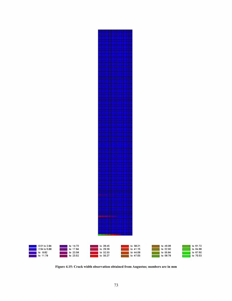
73
Figure 4.15: Crack width observation obtained from Augustus; numbers are in mm

74
Figure 4.16: crack width constraint
4.5.5. Creep
In reinforced concrete structures, the structural members exhibit a long-term static strength that is
significantly lower than the short-term strength. This long-term static strength is observed when
these members are exposed to a sustained stress for a long period of time in air, acid, alkaline, sea
water or other certain environmental exposure. Degradation of the material properties with time
leads to a failure called creep rupture (Al-Salloum and Almusallam 2007).
Creep deformation for steel is generally insignificant, and it can be ignored unless the steel
reinforced structure exposed to extremely high temperatures, such as in the case of a fire (ACI
440.1R 2006).
For the FRP reinforcing bars subjected to a constant load over time, creep deformation leads to a
sudden failure involving reinforcement fracture. This failure happens after a period of time called
endurance time (ACI 440.1R 2006).
Two factors influence the endurance time. The first one is the ratio of sustained tensile stress to
the initial strength of the bars. Sustained tensile stress is the stress caused by unfactored sustained
Strength
constraint
0
1500
3000
4500
6000
7500
9000
10500
12000
13500
0 0.2 0.4 0.6 0.8 1 1.2 1.4 1.6
Wid
th (
mm
)
FRP - vertical reinforcement ratio (%)
Balanced sections
Crack width constraint
Deflection
constraint Feasible zone

75
loads, including dead loads and the sustained portion of the live load. A shorter endurance time
corresponds to a higher ratio of sustained stress to short-term strength. The second factor is the
adverse environmental conditions like high temperature, ultraviolet radiation exposure, high
alkalinity, and wet and dry cycles, or freezing-and-thawing cycles (ACI 440.1R 2006). More
adverse environmental conditions lead to shorter endurance times.
The possibility of a mode of failure consisting of creep rupture in FRP bars depends on the type
of fibers in the FRP material. For example, creep rupture is more common in GFRP bars while
carbon fibers are less susceptible to creep rupture. Therefore, due to the severity of the
consequences associated with the failure caused by bar fracture, the creep constraint should be
considered as an additional constraint in the width- reinforcement ratio diagram for FRP-
reinforced concrete shear walls.
According to the research conducted by Yamaguchi et al. (1998), creep failure of the GFRP bars
depends on the loading time. Balafas and Burgoyne (2012), also proposed the Eq. 4.23 to calculate
the stress level of FRP reinforcement relating to the creep failure which depends on time t, in
hours.
10(1 log )t if f t (4.23)
Where if is the initial FRP strength and tf shows the strength after time t. is a constant number
equal to 0.101 for the GFRP bars which is obtained from a research conducted by Yamaguchi et
al. (1998). B for all types of FRP are mentioned in Table 4.2.
Table 4. 2: Values for variable (1998)
FRP Type
GFRP 0.101
AFRP-Fibra 0.069
AFRP-Technora 0.053
CFRP 0.016

76
Code provisions place an upper limit to the ultimate FRP strength to avoid creep rupture mode of
failure. Code provisions in CSA S806 state that for glass fiber reinforced polymer bars, the million-
hour strength against creep rupture should be more than 35% of ultimate tensile strength. This
strength for the bars in this research is calculated in Eq. 4.24.
min 0.35 1412 494.2tf MPa (4.24)
Comparing the code value to the expression suggested by Balafas and Burgoyne (2012), it is seen
that the code value is slightly less conservative Eq. 4.25.
101412(1 0.101log 1000000) 556.328 492.2tf MPa MPa (4.25)
In this study, creep is caused by the sustained axial load applied to the shear walls. In order to
apply the creep constraint to the width against reinforcement ratio diagram, all shear walls were
modeled in Vector2 using a creep-related ultimate strength of 556.3 MPa instead of their original
ultimate strength, 1412 MPa. Then, the same procedure for the strength constraint in section 4.5.1
is repeated in this section to obtain the creep constraint line.
Figure 4.17 shows the ultimate strength of the walls obtained from the pushover analysis while
using the creep rupture strength for the bars in the modeling. The ultimate strengths of the walls
were compared with the reference ultimate strength (1112.1 kN). Those which are stronger than
the reference wall are shown with the cross markers, and the others are shown with the circles. The
acceptable walls in terms of ultimate creep strength lay above the creep line and vice versa.

77
Figure 4.17: Ultimate strength of the shear walls considering creep rupture strength of the GFRP bars
Figure 4.18 (a) shows how the creep constraint separates the walls with ultimate strength equal to
or more than reference ultimate strength, 1112.1 kN from those which are not strong enough. Then
in Fig. 4.18 (b), the creep constraint is applied to the width against reinforcement ratio diagram to
see its effect on the feasible zone area. It is seen that if the deflection constraint is neglected, creep
rupture constraint has the potential to reduce the feasibility region. Therefore, if a designer meets
the deflection constraint and aims for the allowable crack width , creep fracture considerations are
not a concern.
269387
604
1074
2417
338487
761
1121
3044
400576
900
1600
3600
455656
1024
1821
4098
506727
1136
2020
4545
550792
1237
2200
4949
0
1500
3000
4500
6000
7500
9000
10500
12000
13500
0 0.2 0.4 0.6 0.8 1 1.2 1.4 1.6
Wid
th (
mm
)
FRP - vertical reinforcement ratio (%)

78
(a)
(b)
Figure 4.18: (a) separating line; (b) creep constraint
Strength
constraint
0
1500
3000
4500
6000
7500
9000
10500
12000
13500
0 0.2 0.4 0.6 0.8 1 1.2 1.4 1.6
Wid
th (
mm
)
FRP - vertical reinforcement ratio (%)
Balanced Creep
RuptureCrack
width
Feasible zone
Deflection constraint

79
4.5.6. Cost Function
Determination of the most economical design of the shear walls in the w diagram would not
be possible without including a cost function into this diagram. Such a function must include the
cost of flexural reinforcement and concrete (Yousef A Al-Salloum and Ghulam Husainsiddiqi
1994). Costs of the horizontal reinforcement and formwork were not incorporated into the cost
function. Equation 4.26 demonstrates how these costs are incorporated into the cost function. The
cost function is given by
C( , ) ( (1 )) ( )c gw C w t h C w t h (4.26)
Where cC is the cost of concrete per unit sectional area of concrete per unit height of the shear
wall. gC is the cost of GFRP per unit area of GFRP per unit height of the shear wall for the vertical
reinforcement. The variables w , t and h are the width (mm), thickness (mm), and height (m) of
the wall respectively. The equation can be simplified as follows (Eq. 4.27)
C( , ) ( (1 )) ( )c gw C w t h C w t h
C( , ) ((1 ))c gw C wth C wth
C( , ) (( )g c cw C C wth C wth
C( , ) ( )g c cw C C th w C th w
C( , )w X w Yw (4.27)
X and Y are constant numbers depend on the material costs, wall thickness and height. These
parameters are constant for all of the walls in this study.
( )g c
c
X C C th
Y C th
The unit cost of the materials which are incorporated into the cost function, are shown in Table 4.3
(these costs are obtained from industry). w and t are 200 mm and 27 m for all of the walls.

80
Table 4. 3: Material costs
Material Cost ($/mm2/m)
Concrete Cc=0.00025
GFRP Cg=0.02189
Steel Cs=0.00841
Therefore, the values for X and Y are:
0.02189 0.00025) 200 27 116.856
0.00025 200 27 1 3
)
. 5
( (g c
c
X C C th
Y C th
The cost function for the GFRP reinforced concrete shear walls can be found in Eq. 4.28.
C( , ) 116.856 1.35w w w (4.28)
Where is the vertical, flexural, reinforcement ratio, and w is the wall width (mm).
Equation 4.28 shows that there are several shear walls with various concrete dimensions and
reinforcement but equal cost that can be shown with a line in the width against flexural
reinforcement ratio diagram called the cost function line (Balafas and Burgoyne 2012).
For example, the cost function for the shear walls with the cost of $10000, $15000, and $20000
are shown in Fig. 4.19. Each line shows a many possible wall designs with various reinforcement
ratios and concrete dimensions having the same cost.

81
Figure 4.19: Cost functions for walls with various costs
Having the equation of the cost function (Eq. 4.28), the optimum design solution for GFRP
reinforced concrete shear walls can be found in the width against reinforcement ratio diagram. The
optimum design solution is the most economic design for the shear walls. This optimum solution
is the point or the points where the cost function line meets the feasible zone at the cheapest price
in the width against reinforcement ratio diagram.
In this case, the optimal solution of GFRP reinforced shear walls is located at the intersection of
the crack width constraint and the deflection constraint as shown in Fig. 4.20. The width and the
reinforcement ratio for this wall is 8300 mm and 0.75% respectively. Putting these values in the
Eq. 4.28 the cost of the optimal solution for the GFRP reinforced shear walls is $18400.
C( , ) 116.856 1.35 116.856 0.0075 8300 1.35 8300 $18400w w w (4.29)
0
2000
4000
6000
8000
10000
12000
14000
0 0.2 0.4 0.6 0.8 1 1.2 1.4 1.6
Wid
th (
mm
)
FRP - vertical reinforcement ratio (%)
Cost: $20000
Cost: $15000
Cost: $10000

82
Figure 4.20: Flexural optimal solution for GFRP reinforced walls
Looking at the feasible zone in the w diagram, it is obvious that the optimum design solution
is the first point at the most left bottom side of the feasible zone. Because this point has which the
least width and reinforcement ratio in the feasible zone. However, drawing the cost function line
allows the designers to make sure that there is not any other point in the feasible zone having the
same price. Sometimes there is more than one optimal solution with the same cost, this way the
cost function meets the feasible region in more than 1 point.
As more research results and data on long-term performance of FRP-reinforced structures become
available, and manufacturing processes achieve greater efficiencies, it is expected that the price of
FRP materials decreases. Currently, the price of a GFRP bar is about three times of that of steel
(Table 4.3). Equating the prices of both GFRP and steel, a flatter line for the cost function is
obtained, as shown in Fig. 4.21. The new cost function equation for this case, shear walls with
cheap GFRP bars, is shown in Eq. 4.30.
0
1500
3000
4500
6000
7500
9000
10500
12000
13500
0 0.2 0.4 0.6 0.8 1 1.2 1.4 1.6
Wid
th (
mm
)
FRP - vertical reinforcement ratio (%)
Cost Function
Crack width
constraint
Feasible zone
Deflection constraint
Flexural
optimal
solution

83
C( , )w X w Yw
g sC C
Using the cost in Table 4.3:
0.00841 0.00025) 200 27 44.064
0.00025 200
( ) (
27 1.35
s c
c
X C C th
Y C th
C( , ) 44.064 1.35w w w (4.30)
Figure 4.21: Comparison of the GFRP cost functions affected by the initial price of the bars
In this case with flatter cost function line, the flexural optimum solution is not one point anymore.
In fact, there is a range of shear walls with the same costs which are the optimal design solutions
(Fig. 4.22).
0
2000
4000
6000
8000
10000
12000
14000
0 0.2 0.4 0.6 0.8 1 1.2 1.4 1.6
Wid
th (
mm
)
FRP - vertical reinforcement ratio (%)
GFRP cost function
GFRP cost function (for less expensive GFRP)

84
For example, for two walls at the very end of this range, the costs of the walls are calculated in Eq.
4.31 and Eq. 4.32. The wall at the vertex of the crack width and the deflection constraint has the
width of 8300 mm and the reinforcement ratio of 0.0075. While the other one at the right end of
the flexural optimal solutions range has the width and the reinforcement ratio of 7676 mm and
1.06 percent respectively. The calculation at bellow shows the cost comparison of these two walls.
As expected, the cost of both walls is the same since they are on the same cost function line.
Repeating the same procedure, the middle points should have the same cost as well.
C( , ) 44.064 1.35 44.064 0.0075 8300 1.35 8300 $13900w w w (4.31)
C( , ) 44.064 1.35 44.064 0.0106 7676 1.35 7676 $13900w w w (4.32)
Figure 4.22: Flexural optimal solutions for the GFRP reinforced walls; (considering the same initial price for GFRP and
steel bars)
0
1500
3000
4500
6000
7500
9000
10500
12000
13500
0 0.2 0.4 0.6 0.8 1 1.2 1.4 1.6
Wid
th (
mm
)
FRP - vertical reinforcement ratio (%)
Cost Function
Crack
width
Feasible zoneDeflection
constraint Flexural
optimal
solutions

85
4.5.7. High Strength Concrete
In the design of FRP reinforced shear walls, due to the low elastic modulus of the reinforcement,
deflection at service condition is very critical in comparison to the other constraints. As shown in
Fig. 4.20, the size reduction in the feasible zone caused by this constraint is greater than that
produced by the other variables.
One option to keep the deflections within the allowable limits is the use of high-strength concrete
(Nanni 1993). In general, high-strength concrete (HSC) when used in multistory buildings and
bridges offers superior performance and economy. The concrete stress-strain relationship depends
on its strength. Concrete with higher strength has higher elastic modulus. This provides the
reinforced concrete structures with higher stiffness, which reduces the deflections and leads to
smaller cracks. Also, the strain at peak stress of concrete increases with increment in strength.
However, failure of the high strength concrete is more sudden and brittle in comparison to normal
strength concrete (Ozbakkaloglu and Saatcioglu 2004).
For FRP reinforced concrete elements, the use of high-strength concrete increases the stiffness of
the cracked section. It also leads to a better use of the high-strength properties of FRP bars when
comparing with sections with the normal-strength concrete (GangaRao and Vijay 1997). Hence,
fewer bars can be used in the wall made of high-strength concrete in comparison to the walls made
with normal strength concrete.
Concrete with peak compressive strength exceeding 70 MPa are commonly referred as high-
strength concrete (James G. MacGregor and F.Michael Bartlett 2000). As for the maximum limit,
the provisions in CSA S807 (CSA S807 2010) allow the maximum concrete strength of 80 MPa
in design for FRP reinforced concrete structures.
As shown in Fig. 4.23, the difference between the deflection constraints of the walls with normal
strength and high strength concrete is more obvious for the walls with less reinforcement ratio in
comparison to those in which reinforcement ratio is higher. Since the increment in the concrete
strength is more effective where its area is higher, the reinforcement area is lower.
.

86
Figure 4.23: The effect of high strength concrete on the deflection constraint
Using high strength concrete may affect other structural parameters besides the deflection. For
instance, the crack width limit is another constraint governing the optimal design solution (Fig.
4.20). The effect of the concrete strength on the crack width of the flexural reinforced concrete
members has been investigated by Michèle Thériault and Benmokrane (1998). Their experimental
results show that the crack width is independent of the concrete strength. This constraint is
expected to remain constant in the width against reinforcement ratio diagram.
On the other hand, for a reinforced flexural member with high strength concrete, the balanced
section constraint is more critical than the sections with normal strength concrete. This is because
more reinforcement in tension is needed to balance the compression forces when high-strength
concrete is used. The balanced section line moves to the right in the width against reinforcement
ratio diagram as shown in Fig. 4.24.
Considering the effects of the high strength concrete on the deflection and the balanced section
constraints, the feasible zone area of the FRP reinforced shear walls is changed to the one is shown
in Fig. 4.25
0
1500
3000
4500
6000
7500
9000
10500
12000
13500
0 0.2 0.4 0.6 0.8 1 1.2 1.4 1.6
Wid
th (
mm
)
FRP - vertical reinforcement ratio (%)
Deflection constraint for walls
with high strength concrete
Deflection constraint for walls with
normal strength concrete

87
Figure 4.24: Balanced sections constraints comparison between the sections with high strength and normal strength
concrete
Figure 4.25: feasible zone for walls with high strength concrete
0
1500
3000
4500
6000
7500
9000
10500
12000
13500
0 0.2 0.4 0.6 0.8 1 1.2 1.4 1.6
Wid
th (
mm
)
FRP - vertical reinforcement (%)
Balance sections
(normal strength
concrete)
Balanced sections
(high strength
concrete)
Strength
constraint
Balanced sections
Crack width
constraint
Creep rupture
constraint
0
1500
3000
4500
6000
7500
9000
10500
12000
13500
0 0.2 0.4 0.6 0.8 1 1.2 1.4 1.6
Wid
th (
mm
)
FRP - vertical reinforcement (%)
Feasible zone
Crack width
constraint
Deflection

88
Having the feasible zone determined, the optimal design solution for the shear walls with high
strength concrete can be found by applying the cost function into the width against reinforcement
ratio diagram. As for the cost function, the 80 MPa concrete which is used in this research for high
strength concrete is more expensive than normal strength concrete (40 MPa). The new cost
function is as Eq. 33.
C( , )w X w Yw
0.02189 0.000327) 200 27 116.44
0.000327 200 27 1.7 8
( ) (
65
g c
c
X C C th
Y C th
C( , ) 116.844 1.7658w w w (4.33)
Figure 4.26 shows the effect of high strength concrete on the cost function line in the width against
reinforcement ratio diagram. Although the cost function line for the shear walls with high strength
concrete is flatter, it is not affected by the concrete strength change significantly. Because the
concrete cost, in general, is negligible in comparison to reinforcement cost as shown in Table 4.3.
Figure 4.26: Cost function comparison for shear walls with normal strength and high strength concrete
0
2000
4000
6000
8000
10000
12000
14000
0 0.2 0.4 0.6 0.8 1 1.2 1.4 1.6
Wid
th (
mm
)
FRP - vertical reinforcement ratio (%)
Cost function for
walls with normal
strength conrete
Cost function for
walls with high

89
The optimal design solution for the GFRP reinforced shear walls with high strength concrete
(compressive strength= 80 MPa) is shown in Fig. 4.27.
Figure 4.27: Flexural optimal solution for GFRP reinforced shear walls with high strength concrete
Figure 4.27 shows that even by increasing the strength of the concrete, the optimal design is still
governed by the deflection and crack width constraints.
The optimal design solution for the walls with high strength concrete has the width and the
reinforcement ratio of 8100 mm and 0.0075 respectively. The cost of the optimal design solution
for the walls with high strength concrete is calculated below using Eq. 4.33. The optimal design
solution in this case is more expensive than the case with normal strength concrete.
C( , ) 116.844 1.7658 116.844 0.0075 8100 1.7658 8100 $21000w w w (4.34)
Crack width
constraint
0
1500
3000
4500
6000
7500
9000
10500
12000
13500
0 0.2 0.4 0.6 0.8 1 1.2 1.4 1.6
Wid
th (
mm
)
FRP - vertical reinforcement (%)
Feasible zone
Crack width
constraint
Deflection
Cost function
Flexural
optimal
solution

90
4.5.8. Sensitivity Study of Deflection
For all GFRP reinforced shear walls investigated, even those with high strength concrete, the
deflection limits at service condition governs the choice of the optimal solution. As mentioned
previously in section 4.5.3, the deflection constraint used so far is based on the drift limit of 1/ 500
the story height determined by the provisions of National Building Code of Canada (NBCC 2015
). In this section, the influence of the deflection constraint is investigated using a more relaxed
deflection limit of / 300h provided by British Standards institution and European Committee
Standardization 1991.
Figure 4.28 shows that the effect of the deflection limit change on the deflection constraint. It
demonstrates that using a more relaxed deflection limit, / 300h , instead of / 500h leads to a
stretch in the feasible zone area.
Figure 4.28: The effect of deflection limit on the deflection constraint
The feasible zone and the flexural optimum solutions for the GFRP reinforced shear walls
considering / 300h as the limit for service deflections are shown in Fig. 4.29 and Fig. 4.30
0
1500
3000
4500
6000
7500
9000
10500
12000
13500
0 0.2 0.4 0.6 0.8 1 1.2 1.4 1.6
Wid
th (
mm
)
FRP - vertical reinforcement (%)
Deflection constraint
( Deflection limit= h/500)
Deflection constraint
(Deflection limit= h/300)
Feasible zone

91
respectively. Figure 4.30 shows the optimal design solution has the width and the reinforcement
ratio of 7900 mm and 0.0075 respectively. The cost of the optimal solution in this case is calculated
using Eq. 4.35.
C( , ) 116.856 1.35 116.856 0.0075 7900 1.35 7900 $17000w w w (4.35)
Figure 4.29: Feasible zone for the shear walls with deflection limit=h/300
Strength
constraint
Deflections
constraint
Crack width
constraint
Creep rupture
constraintBalanced
sections
0
1500
3000
4500
6000
7500
9000
10500
12000
13500
0 0.2 0.4 0.6 0.8 1 1.2 1.4 1.6
Wid
th (
mm
)
FRP - vertical reinforcement (%)
Feasible zone

92
Figure 4.30: Flexural optimal solution for the shear walls with deflection limit=h/300
4.5.9. Bond
An additional factor that significantly influences the crack widths in RC members is the bond
between reinforcing bars and concrete (Mazaheripour et al. 2013 and Tighiouart et al. 1998). For
the flexural members with FRP bars having a lower elastic modulus in comparison to steel, the
low bond strength is a disadvantage; since it significantly increases the crack widths (Balafas and
Burgoyne 2012). This leads to a more critical crack width constraint and reduces the size of the
feasible zone. Therefore, increasing the bond strength seems effective to get a more economic
design solution for the GFRP reinforced concrete shear walls. Adding ribs and wraps to the surface
of FRP bars improves the bond strength.
In this research, a simplified analysis is conducted to investigate the effect of the bond on the crack
width of the walls. The bond-model used in this research for the GFRP bars is the Eligehausen
model as discussed in chapter 3. This bond model is developed for sanded bars. Perfect bond, thus,
is assumed between the FRP bars and the surrounding concrete to study the upper ceiling for the
bond strength – in this way, intermediate cases that include ribbed surface bars will be covered.
Crack width
constraint
Deflection
constraint
0
1500
3000
4500
6000
7500
9000
10500
12000
13500
0 0.2 0.4 0.6 0.8 1 1.2 1.4 1.6
Wid
th (
mm
)
FRP - vertical reinforcement (%)
Feasible zoneFeasible zone
Cost functionFlexural
optimal
solution

93
In the modeling, the perfect bond is achieved using the common-node approach. Figure 4.31 shows
that the perfect bond of the GFRP bars to the concrete leads the crack width constraint to be less
critical moving to the left in the width against flexural reinforcement ratio diagram. That extends
the feasible zone area and leads to a more economical solution in comparison to the flexural
optimal solution for the GFRP reinforced shear walls with imperfect bond for the reinforcement.
Figure 4.32 and Fig. 4.33 show the feasible zone and the best solution for the walls with perfect
bond between concrete and reinforcement respectively.
Figure 4.31: Crack width constraint comparison between walls with perfect bond and intermediate one for GFRP bars
Crack width
constraint
0
1500
3000
4500
6000
7500
9000
10500
12000
13500
0 0.2 0.4 0.6 0.8 1 1.2 1.4 1.6
Wid
th (
mm
)
FRP - vertical reinforcement (%)
Crack width
constraint
( perfect bond)

94
Figure 4.32: Feasible zone area for GFRP reinforced shear walls with perfect bond for reinforcement
Figure 4.33: Flexural optimal solution for GFRP reinforced shear walls with perfect bond for reinforcement
Balanced sections
Deflections
constraint
Crack width
constraint
Creep rupture
constraint
0
1500
3000
4500
6000
7500
9000
10500
12000
13500
0 0.2 0.4 0.6 0.8 1 1.2 1.4 1.6
Wid
th (
mm
)
FRP - vertical reinforcement ratio(%)
Feasible zone
Strength constraint
Deflection constraint
Crack width
constraint
0
1500
3000
4500
6000
7500
9000
10500
12000
13500
0 0.2 0.4 0.6 0.8 1 1.2 1.4 1.6
Wid
th (
mm
)
FRP - vertical reinforcement ratio(%)
Feasible zone
Deflection constraint
Cost function
Flexuraloptimal solution

95
According to Fig. 4.33, the flexural optimal solution width is 8600 mm, and its reinforcement
ratio is 0.62 percent. Therefore, the cost of the best solution when increasing the bond to the
perfect bond is $17840.8 as calculated in Eq. 4.36.
( , ) 116.856 1.35 116.856*0.0062*8600 1.35*8600 $17800C w p w w (4. 36)
Table 4.4 compares the cost of the optimal design solutions for FRP reinforced shear walls
considering the affecting factors on the design constraints. It shows that the reduction in the initial
cost of GFRP bars leads to the most economic design solution for the shear walls reinforced with
these bars. Increasing the bond between reinforcement and concrete as well as relaxing the
deflection limit to a higher one leads to almost the same cost for the optimal design solution.
However, using high strength concrete is not beneficial in terms of cost for the flexural optimal
design solution of the shear walls under study.
Table 4. 4: Comparison of the optimal design solution costs (GFRP reinforced shear walls)
GFRP reinforced concrete shear walls Cost of the optimal design solutions ($)
GFRP reinforced concrete shear walls
18400
GFRP reinforced concrete shear walls with inexpensive GFRP bars
13900
GFRP reinforced concrete shear walls with high strength concrete
21400
GFRP reinforced concrete shear walls with relaxed deflection limit
17500
GFRP reinforced concrete shear walls with perfect bond
17800

96
4.6. Shear Walls with Other Heights, Reinforcement Configurations and Axial
Loads
In this study, the parametric analysis was conducted on the walls with the same height and
thickness of 27 and 0.2 meters, and the same horizontal reinforcement of 1.5 percent. As discussed
in previous sections, the minimum thickness is required to avoid very thin walls. Also for the shear
reinforcement, there is a minimum ratio should be met for controlling the mode of failure and
preventing shear failure. Therefore, assigning various values to these two variables does not have
any critical effect on the flexural design of the shear walls if their minimum requirements are met.
However, there are some important points about the height, reinforcement configuration, as well
as the axial load of the walls worth investigating. Because any changes in these parameters affects
the flexural response of the shear wall. For the walls with different heights rather than 27 meters,
other reinforcement configurations rather than evenly distributed bars, as well as other axial load
rather than seven percent of the section capacity, the results of this research can be expanded. To
this aim, the effect of these two parameters on the flexural design constraints should be
investigated.
The first constraint is the ultimate strength constraint that should be investigated. To investigate
this constraint for walls with the heights rather than 27 meters, the reference wall is kept constant.
Considering the cantilever behavior of the shear walls, if taller walls are analyzed, ultimate loads
of the walls will decrease. Thus, fewer walls will have the same or higher strength than the
reference ultimate strength. Consequently, the strength constraint goes upper in the width against
reinforcement ratio diagram. This constraint, therefore, becomes more critical and reduces the
feasible zone area. On the contrary, shear walls in shorter buildings have higher ultimate strength;
therefore, most of the walls are meeting the strength constraint criteria and lay at the top of this
constraint line in the width against reinforcement ratio diagram. So, the strength constraint is not
very critical in this case, and the feasible zone will be stretched.
As for the balanced reinforcement ratio, the minimum reinforcement ratio required to avoid brittle
mode of failure is obtained from Eq. 4.14. This ratio remains constant by changing the height of
the wall because it only depends on the cross-sectional properties. Therefore, the line related to
this constraint remains constant at the same location in the width- reinforcement ratio diagram.

97
The other constraint affecting the flexural design of the shear walls is the deflection at service
condition. The working load obtained from the reference wall performance in the service condition
is considered to be constant. Keeping the widths constant, an increment in the heights of the walls
leads to more slender walls. The displacements are larger for the slender walls. Therefore, fewer
walls will remain within the limit of the National Building Code of Canada (NBCC 2015 ) which
is h/500 of the wall height. This way, the deflection constraint will move upper limiting the feasible
zone area more for the taller walls; however, this constraint is less critical and will stretch the
feasible zone for the walls which are shorter than 27000 mm.
The crack width constraint is another service condition should be checked for the shear walls with
the heights rather than 27 meters. The crack widths will be increased for the shear wall if the
slenderness of the wall is increased. Because the deflections are larger in the higher walls, the
cracks open wider. Therefore, fewer walls remain in the crack width limit. The crack width line is
moved to the right in the width against reinforcement ratio diagram for the taller walls and limits
the feasible zone more. For shorter walls, the crack widths are smaller, so the feasible zone will be
stretched.
The last constraint should be investigated is the creep constraint. The effect of the wall height
change on the creep constraint is exactly as same as the effect of that on the strength constraint,
because these two constraints are created using the same procedure. The only difference is the
strength used for the reinforcement in the modeling. For the creep constraint, the creep strength is
used instead of the ultimate strength of the reinforcement. Therefore, for shorter walls, the creep
width constraint moves lower which is less critical, and vice versa.
The cost function line includes the height variable. Therefore, it will be modified for the shear
walls with different heights.
In this parametric study, reinforcement is considered to be distributed evenly in the cross section
of the walls. For the walls with concentrated reinforcement at the boundaries, the ultimate load
capacity of the walls is higher. Therefore, more walls pass the strength criteria leading to a more
relaxed strength constraint and larger feasible zone in the width against reinforcement ratio
diagram. With the same reason, creep constraint is more relaxed for the walls with concentrated
reinforcement in the boundaries. On the other hand, when the reinforcement is concentrated in the

98
boundaries, there is not enough reinforcement for bridging the cracks in the web of the wall; thus,
cracks are wider in comparison to the walls with distributed reinforcement.
When it comes to the effect of the various axial loads on the flexural design constraint and feasible
zone area, increment in axial load increases the strength of the walls. This leads to a more relax
strength and creep constraints. Also, increasing the axial load leads to smaller deflections and
consequently reduced the crack widths in the shear wall. Therefore, the design constraints at
service are not critical when the axial load is increased. Considering all of the changes in the design
constraints, increasing the axial load leads to a larger feasible zone and therefore more economic
optimal design solutions.
5. Chapter 5. Economic Design of Steel-Reinforced RC Shear Walls
5.1. GFRP Reinforced Shear Walls against Walls with Steel Reinforcement
In this chapter, the width vs. reinforcement ratio diagram and the flexural optimum solutions found
for the FRP reinforced shear walls are compared to those of steel reinforced shear walls. It is
expected that this comparison will give designers an overview about the choice of reinforcement
considering the constraints noted earlier. The design constraints for steel reinforced shear walls
are investigated in following sections.
5.2. Strength Constraint for Steel Reinforced Shear Walls
Following the same procedure done for the GFRP reinforced shear walls in section 4.5.1, the
ultimate strengths of some of the shear walls with steel reinforcement are shown in Fig. 5.1. These
strengths are obtained from the pushover analysis of the walls. Then the comparisons were made
between each wall ultimate strength and the reference ultimate strength (1112 kN). Subsequently,
the strength constraint is shown in Fig. 5.2; the ultimate strengths are divided to acceptable (cross
marker) and inacceptable (circle marker) shear walls in part (a), then the feasible zone created with
this constraint is shown in part (b) for the steel reinforced shear walls.

99
Figure 5. 1: Ultimate strength of the steel reinforced shear walls
(a)
294419
652
1059
2604
370534
816
1303
3095
450634
992
1801
3642
522731
1112
1944
4081
587825
1248
2383
4662
648904
1380
2482
5145
0
1500
3000
4500
6000
7500
9000
10500
12000
13500
0 0.2 0.4 0.6 0.8 1 1.2 1.4 1.6
Wid
th (
mm
)
Steel - vertical reinforcement ratio (%)

100
(b)
Figure 5. 2: (a) separating line; (b) strength constraint
Figure 5.3 shows the comparison between the strength constraints of steel and GFRP reinforced
shear walls. Since FRP reinforcement has higher ultimate strength in comparison to the steel
reinforcement, FRP-reinforced shear walls have ultimate strengths higher than what exhibited by
steel-reinforced shear walls considering the concrete dimensions and reinforcement ratios the same
for both groups. Results show that because the ultimate strengths of the steel reinforced shear walls
are relatively low, more walls will not have higher strength than the reference wall strength when
compared with the walls with GFRP reinforcement. Therefore, the strength constraint of the steel
reinforced shear walls is higher, more critical, than the GFRP reinforced shear walls in the width
against reinforcement ratio diagram.
Strength
constraint
0
1500
3000
4500
6000
7500
9000
10500
12000
13500
0 0.2 0.4 0.6 0.8 1 1.2 1.4 1.6
Wid
th (
mm
)
Steel - vertical reinforcement ratio (%)
Feasible zone

101
Figure 5. 3: Comparison of ultimate strength constraints of steel and GFRP reinforced concrete shear walls
5.3. Minimum and Balanced Reinforcement Ratios for Steel Reinforced Shear
Walls
As for the steel reinforcement ratio, according to the provisions of CSA A23.3 (CSA A23.3 2004),
there are minimum and maximum limits for the reinforcement ratio that should be considered in
the flexural design of the steel reinforced concrete shear walls. The following paragraphs are
discussing the minimum and the balanced reinforcement ratios determined in this code.
According to the provisions of CSA A23.3 (CSA A23.3 2004), the minimum reinforcement area
for each flexural member with tensile reinforcement can be obtained from Eq. 5.1. This minimum
reinforcement area is required to avoid a sudden failure caused by excessive cracking. For the
flexural members with reinforcement area less than the minimum area provided in the Eq. 5.1 the
flexural behavior is like plain concrete sections that fail rapidly as soon as the cracking moment is
reached. This equation is used to ensure the section has the minimum required area of the tension
reinforcement.
Strength
constraint-GFRP
reinforced walls
Strength
constraint- Steel
reinforced walls
Feasible zone
0
1500
3000
4500
6000
7500
9000
10500
12000
13500
0 0.2 0.4 0.6 0.8 1 1.2 1.4 1.6
Wid
th (
mm
)
vertical reinforcement ratio (%)

102
,min
0.2 'cs
y
fA w t
f (5. 1)
Where ’cf and yf are the concrete compressive strength and the steel yield strength respectively
in MPa. w and t are the shear wall cross section dimensions in mm.
On the other hand, the maximum reinforcement ratio, also called the balanced reinforcement, for
the steel reinforced shear wall can be obtained from Eq. 5.2. This limit is shown with a line in the
width against reinforcement ratio diagram which divides the graphs to two parts. The walls lay on
this line have the balanced sections in which the concrete crushes at the same time as steel yields
which is known as the balance failure. The sections lay at the left-hand side of the balanced section
line called under reinforced sections. They develop tension failure as their mode of failure,
reinforcement yields before concrete reaches its limiting compressive strain. On the contrary, the
over-reinforced sections are the ones with reinforcement more than what balanced sections have.
These sections will fail by crushing of concrete before experiencing yielding of steel; this mode of
failure is not desirable for steel reinforced shear walls. Therefore, the balanced, maximum,
reinforcement ratio ensures the yielding of tension reinforcement prior to the crushing of the
concrete, which is desirable for ductile behavior.
1 1 '( )c c cu
b
s y cu y
f
f
(5. 2)
Where ’cf and yf are in Mpa. y is the yielding strain of steel equal to 0.002. The other
parameters are defined previously. Figure 5.4 shows these two steel reinforcement limits, the
minimum and the balanced reinforcement, in the width against reinforcement ratio diagram. The
feasible zone created with the minimum and the maximum reinforcement ratios and the strength
constraint is shown in Fig. 5.5.

103
Figure 5. 4: Reinforcement limits for the steel reinforced shear walls
Figure 5. 5: Minimum and maximum reinforcement constraints
Strength
constraint
Balanced
reinfrocementMinimum
reinforcement
Excessive
cracking
Under
reinforced
sections: steel
yeilds before
concrete
crushesOver reinfoced
sections:
concrete
crushes before
steel yeilds
0
1500
3000
4500
6000
7500
9000
10500
12000
13500
0 1 2 3 4 5 6
Wid
th (
mm
)
Steel - vertical reinforcement ratio (%)
Strength
constraint
Minimum
reinforcement
Steel yeilding
before concrete
crushing
0
1500
3000
4500
6000
7500
9000
10500
12000
13500
0 1 2 3 4 5
Wid
th (
mm
)
Steel - vertical reinforcement ratio (%)
Feasible zone
Maximum reinforcement

104
5.4. Deflection Constraint for Steel Reinforced Shear Walls
When it comes to the deflection limit for the steel reinforced concrete shear walls, this limit is as
same as the one used for the GFRP reinforced walls. National Building Code of Canada (NBCC
2015 ) limits the maximum relative deflection of the top and bottom of the walls under non-seismic
loads to 1/500 of the wall height. However, since the modulus of elasticity of steel reinforcement
is more than 2 times of that of GFRP reinforcement (Table 4.3), the steel reinforced shear walls
are not as flexible as GFRP reinforced ones. Therefore, the deflections in steel reinforced shear
walls are not as large as those observed in GFRP reinforced shear walls. This leads the deflection
constraint at service load in the steel reinforced shear walls to not be as critical as it is for the walls
with GFRP bars. Figure 5.6 shows the comparison between the deflection constraint of steel and
GFRP reinforced shear walls. The modulus of elasticity of FRP is lower, so the deflection
constraint for the walls with this type of reinforcement is more critical, and it minimizes the
feasible zone more.
Figure 5. 6: Deflection constraint comparison between steel and GFRP reinforced shear walls
Deflection
constraint-GFRP
reinforced walls
Deflection
constraint-Steel
reinforced walls
Feasible zone
0
1500
3000
4500
6000
7500
9000
10500
12000
13500
0 0.2 0.4 0.6 0.8 1 1.2 1.4 1.6
Wid
th (
mm
)
Vertical reinforcement ratio (%)

105
The width against reinforcement ratio diagram for the steel reinforced shear walls including the
deflection constraint is shown in Fig. 5.7.
Figure 5. 7: Deflection constraint
5.5. Crack Width Constraint for Steel Reinforced Shear Walls
As for the other serviceability constraint, the crack width limit for the steel reinforced concrete
shear walls, as mentioned in section 4.5.4, was considered 0.3 mm for exterior exposures and 0.4
mm for interior exposure. These limits are determined according to the provisions of ACI 318
(ACI 318M 2008) and CSA A23.3 (CSA A23.3 2004). The crack width constraint in shear walls
with steel reinforcement is not as critical as it is for the GFRP reinforce shear walls. Figure 5.8
shows the comparison between the crack width constraints. It shows that the minimum
Strength
constraintMinimum
reinforcement
Deflections
constraint
0
1500
3000
4500
6000
7500
9000
10500
12000
13500
0 0.2 0.4 0.6 0.8 1 1.2 1.4 1.6
Wid
th (
mm
)
Steel - vertical reinforcement ratio (%)
Feasible zone
Deflection constraint

106
reinforcement ratio required to control the crack widths in shear walls with steel reinforcement is
two third of that of steel reinforced shear walls.
Figure 5. 8: Crack width comparison between shear walls with steel and GFRP reinforcement
The w diagram including the crack width constraint for the steel reinforced shear walls is
shown in Fig. 5.9.
On the other hand, opposed to the GFRP reinforced shear walls, creep rupture is ignored for the
steel reinforcement in the concrete shear walls. Because according to the provisions of ACI 440
(ACI 440.1R 2006) design guide and the study conducted by Balafas and Burgoyne (2004) creep
of steel reinforcement is negligible.
Therefore, since there is no other constraint to investigate, the feasible region for the steel
reinforced concrete shear wall is the one shown in Fig. 5.9.
Crack width
constraint -Steel
reinforced walls
0
1500
3000
4500
6000
7500
9000
10500
12000
13500
0 0.2 0.4 0.6 0.8 1 1.2 1.4 1.6
Wid
th (
mm
)
Crack width
constraint -GFRP
reinforced walls

107
Figure 5. 9: Feasible zone for steel reinforced shear walls
5.6. Cost Function for Steel Reinforced Concrete Shear Walls
The cost function for the steel reinforced concrete shear wall is the one previously mentioned in
Eq. 4.30. Based on the geometry of the feasible zone, the optimal design solution is either the two
points shown in Fig. 5.10 (a) or the range of points shown in Fig. 5.10 (b). The costs of the lines
passing through these points are calculated as follow to determine the most economical solution.
For the first case shown in Fig. 5.10 (a), there are two flexural optimal solutions having the same
cost. The first one has the width of 6200 mm, and the reinforcement ratio of 1.6 percent. The other
wall’s width and flexural reinforcement ratio are 8113.7 mm and 0.005 respectively. The costs of
these two walls are calculated in Eq. 5.3 and Eq. 5.4 respectively.
C( , ) 44.064 0.016 6200 1.35 6200 $12700w (5. 3)
C( , ) 44.064 0.005 8113.7 1.35 8113.7 $12700w (5. 4)
Strength
constraintMinimum
reinforcement
Crack width
constraint
0
1500
3000
4500
6000
7500
9000
10500
12000
13500
0 0.2 0.4 0.6 0.8 1 1.2 1.4 1.6
Wid
th (
mm
)
Steel - vertical reinforcement ratio (%)
Deflection
constraint
Feasible zone

108
On the other hand, the cost of one of the middle points in the range of flexural optimal solutions
shown in Fig. 5.10 (b) is calculated in Eq. 5.5. The width and the reinforcement ratio for this wall
are 6900 mm and 0.009 respectively.
C( , ) 44.064 0.009 6900 1.35 6900 $12000w (5. 5)
Therefore, case two with the range of flexural optimal solutions is more economic. All the walls
shown in this range are acceptable as the optimal design solutions for the steel reinforced concrete
shear wall.
(a)

109
(b)
Figure 5. 10: The optimal design solutions for the steel reinforced shear walls
The optimal design solution of the steel reinforced shear walls is cheaper than that of shear walls with FRP
reinforcement as shown in Table 5.1. However, there are some cost related factors not considered in this
analysis. For example, light weight of FRP bars leads to cheaper transportation, cutting and handling of
FRP bars in comparison to the conventional steel reinforcement. Also, the steel corrosion threatens the
durability of concrete structures. Thus, the additional money spent on improving the durability of
steel reinforced concrete structures can be enormous in comparison to the concrete structures
reinforced with FRP bars.
Table 5. 1: Comparison of the optimal design solution costs (GFRP and Steel reinforced shear walls)
Shear walls Cost of the optimal design solutions ($)
GFRP reinforced concrete shear walls 18400
Steel reinforced concrete shear walls 12000

110
6. Chapter 6. Summary and Conclusions
6.1. Summary
A finite-element (FE) analysis model for FRP-reinforced concrete slender walls was developed
using a finite-element program called VecTor2. Suitable models for material behavior (concrete,
steel, and FRP) were used. A comparison was made between the smeared and the discrete types of
reinforcement modeling, finding that both lead to comparable results. A sensitivity study on the
mesh size was conducted to ensure that the results of the model were stable and independent from
the element size.
The VecTor2 model was validated with the experimental results obtained from three glass FRP
(GFRP)- reinforced concrete shear walls tested at the University of Sherbrook by Mohamed et al.
(2013). These walls were tested to failure under lateral cyclic loading and constant axial loads. The
analysis model was shown to be able to predict the flexural strength of all specimens with
reasonable accuracy (less than 11%). Also, there was a good agreement between the maximum
displacements of the walls obtained from VecTor2 compared to the measured results. The analysis
models were capable of predicting the failure mode of the shear walls. For all the GFRP shear
walls, the mode of failure was concrete crushing like what observed in the experiments. The crack
propagation and the crack width were also well represented by the model.
After validation with an acceptable level of accuracy, the analysis model was used in a parametric
study investigating the influence of typical design constraints through a diagram of the ratio of
flexural reinforcement vs. wall width.
The case study was a 9-storey reinforced concrete building with a height of 27 m. The shear walls
investigated in this research were one of the interior structural walls in this building which were
classified as slender walls. The design constraints investigated were strength, balanced sections,
deflections, crack width and creep. These constraints were chosen since they are typical design
parameters found in practice, and can illustrate the differences between the design principles of
FRP reinforced shear walls with the design principles of the shear walls reinforced with steel rebar.
Investigation of these design constraints led to the determination of a feasible design region for
the FRP reinforced shear walls.

111
After determination of the most critical design constraint, some of the parameters which affect the
governing constraints and the cost function of GFRP reinforced shear walls were investigated. For
example, since GFRP reinforced shear walls are not economic on the first-cost basis, the initial
price of the GFRP bars was reduced to the price of steel bars to determine its effect on the economic
optimal design solution. Also, high strength concrete was used to reduce the excessive deflections,
which was a critical constraint for GFRP reinforced shear walls. The deflection limit was another
parameter increased and its effect on the design feasible zone was investigated. The bond between
concrete and reinforcement was also investigated.
A similar analysis was conducted for steel reinforced shear walls, and comparisons were made
between the design constraints and the optimal design solutions of the FRP- and steel-reinforced
shear walls. This comparison was made to give the designers an overview about the choice of
reinforcement considering the constraints noted above.
6.2. Conclusions
The following conclusions were drawn from this investigation:
• The finite-element implementation of the Modified Compression Field Theory proved its
applicability to simulate the behavior of FRP-reinforced concrete shear walls with
reasonable accuracy, in terms of strength, deflection, crack development, and mode of
failure;
• In GFRP reinforced shear walls, due to the relatively high flexibility of GFRP, deflections
and crack width constraints at service condition governed the feasible zone. Strength was
not a critical constraint for these shear walls since the ultimate strength of the GFRP bars
is high. Creep constraint was not critical as well because the creep-related ultimate strength
is relatively high for GFRP bars;
• By assuming a reduced initial cost for GFRP bars, the governing constraints of the feasible
zone were still the deflection and crack width constraints. The optimal design solutions in
this case were less expensive in comparison to the optimum design solution of the case
with the original initial price of GFRP bars, and include more possibilities for wall size
with the same cost;

112
• Using high-strength concrete led to smaller deflections, which were easier to keep within
allowable limits. Therefore, the deflection constraint was not as critical as it was for the
walls with normal strength concrete. Walls with high strength concrete have a more critical
balanced section line as well. However, crack width constraint is still the governing
constraint of the feasible zone. In this case, the optimal design solution was more expensive
in comparison to the original case. Therefore, using stronger concrete did not bring
significant benefits for the optimal design solution;
• By increasing the deflection limit (using codes of construction different from the NBCC),
the deflection constraint was not critical in comparison to the original case. The feasible
zone size was increased, and the optimal design solution was cheaper with smaller width
in this case.
• Increasing the bond between reinforcement and concrete relaxed the crack width constraint
and increased the feasible zone area. Increasing the bond strength was, thus, beneficial
leading to a more economic design solution with less reinforcement area required.
• The flexural optimal design solution for the shear walls with steel reinforcement was not
governed by the deflection constraint. The strength constraint controlled the design of these
walls. Although the initial cost of GFRP reinforcement is higher than steel by almost 3
times, the optimal design solution of the GFRP reinforced shear wall was marginally, less
than 2 times, more expensive than that of steel reinforced shear walls.
• Although slightly different for shear walls with different types of reinforcement, the
optimal design solutions for both GFRP and steel reinforced walls had height-to-width
aspect ratios between 3 to 4. This fact should be taken into the consideration in design
calculation.

113
6.3. Recommendations for Future Work
Some aspects that should be considered for further work are discussed below:
a) Parametric studies for the economic design of the squat walls reinforced with GFRP bars
with different aspect ratios can be conducted. Squat shear walls have completely different
behavior compared to slender shear walls; squat shear wall behavior is dominated by shear
while in slender shear walls flexural behavior is dominating.
b) Effect of different levels of axial load can be investigated. Different values of axial load
leads to different flexural responses for the shear walls. In this study, the axial load was
considered constant as seven percent of the cross section capacity. The effect of higher and
lower axial loads on the flexural performance of the shear walls with FRP bars should be
investigated.
c) The economic design of the shear walls with other types of FRP reinforcement, such as
carbon, basalt, etc, can be conducted. Although GFRP bars are the cheapest type of FRP
reinforcing bars, some superior properties of other FRP bars may lead to more economic
optimal design solutions.
These proposed studies would allow better assessments in establishing the design guidelines
required for GFRP-reinforced shear walls.

114
References
ACI 318M. 1989. "ACI Committee 318; Building Code Requirements for Reinforced Concrete
(1989)."
ACI 318M. 2008. "ACI Committee 318; Building Code Requirements for Reinforced Concrete
(2008)."
ACI 440.1R. 2006. "ACI Committee 440; Guide for the Design and Construction of Structural
Concrete Reinforced with FRP Bars(2006).".
Almusallam, Tarek H., Yousef A. Al-Salloum, SH Alsayed and Mohammed A. Amjad. 1997.
"Behavior of Concrete Beams Doubly Reinforced by FRP Bars." 2:471-478.
Al-Salloum, Yousef A. and Tarek H. Almusallam. 2007. "Creep Effect on the Behavior of
Concrete Beams Reinforced with GFRP Bars Subjected to Different Environments."
Construction and Building Materials 21(7):1510-1519. doi:
https://doi.org/10.1016/j.conbuildmat.2006.05.008.
Bakis, Charles E., Lawrence C. Bank, VLet Brown, El Cosenza, JF Davalos, JJ Lesko, A.
Machida, SH Rizkalla and TC Triantafillou. 2002. "Fiber-Reinforced Polymer Composites
for construction—State-of-the-Art Review." Journal of Composites for Construction
6(2):73-87.
Balafas, I. and CJ Burgoyne. 2004. "Economic Viability of Structures with FRP Reinforcement
and Prestress.".
Balafas, Ioannis and Chris J. Burgoyne. 2012. "Economic Design of Beams with FRP Rebar Or
Prestress." Magazine of Concrete Research 64(10):885-898.

115
Bentz, EC. 2003. "Augustus: Finite Element Post-Processor for VecTor2 and TRIX."
University of Toronto, Toronto, ON, Canada.
Burgoyne, Chris and Ioannis Balafas. 2007. "Why is FRP Not a Financial Success.".
Chakrabarty, BK. 1992. "Model for Optimal Design of Reinforced Concrete Beam." Journal of
Structural Engineering 118(11):3238-3242.
Clough, Ray W. 1980. "The Finite Element Method After Twenty-Five Years: A Personal
View." Computers & Structures 12(4):361-370.
Cook, Robert D. 1994. Finite Element Modeling for Stress Analysis.Wiley.
Cortés-Puentes, W. L. and Dan Palermo. 2011. "Modeling of RC Shear Walls Retrofitted with
Steel Plates Or FRP Sheets." Journal of Structural Engineering 138(5):602-612.
CSA A23.3. 2004. Canadian Standards Association; Design of Concrete Structures(2004).
CSA S806. 2012. Canadian Standards Association; Specification for Fibre Reinforced
Polymers (2012).Canadian Standards Association.
CSA S807. 2010. Canadian Standards Association; Specification for Fibre Reinforced
Polymers(2010).
Deitz, D. H., I. E. Harik and H. Gesund. 2003. "Physical Properties of Glass Fiber Reinforced
Polymer Rebars in Compression." Journal of Composites for Construction 7(4):363-366
(http://login.ezproxy.library.ualberta.ca/login?url=http://search.ebscohost.com/login.aspx?
direct=true&db=bth&AN=11092516&site=eds-live&scope=site). doi:
10.1061/(ASCE)1090-0268(2003)7:4(363).

116
Ehsani, MR. 1993. "Glass-Fiber Reinforcing Bars." Alternative Materials for the Reinforcement
and Prestressing of Concrete, JL Clarke, Blackie Academic & Professional, London,
England:35-54.
Erki, MA and SH Rizkalla. 1993. "FRP Reinforcement for Concrete Structures." Concrete
International-Detroit- 15:48-48.
Fintel, Mark and M. Fintel. 1995. "Performance of Buildings with Shear Walls in Earthquakes
of the Last Thirty Years." PCI Journal 40(3):62-80.
Foster, Stephen J. and Peter Marti. 2003. "Cracked Membrane Model: Finite Element
Implementation." Journal of Structural Engineering 129(9):1155-1163.
GangaRao, HVS and PV Vijay. 1997. "Design of Concrete Members Reinforced with GFRP
Bars." 1:143-150.
Griffis, Lawrence G. 2003. "Serviceability Limit States Under Wind Load.".
James G. MacGregor and F.Michael Bartlett. 2000. Reinforced Concrete: Mechanics and
Design, First Canadian Ed.Scarborough, Ont: Prentice Hall: .
Kassem, Chakib, Sabry F. Ahmed and Brahim Benmokrane. 2011. "Evaluation of Flexural
Behavior and Serviceability Performance of Concrete Beams Reinforced with FRP Bars."
Journal of Composites for Construction 15(5):682-695. doi: 10.1061/(ASCE)CC.1943-
5614.0000216.
Kessler, RJ and RG Powers. 1988. Corrosion of Epoxy Coated Rebar, Keys Segmental Bridges,
Monroe County.Florida Department of Transportation, Materials Office.

117
Kirsch, Uri. 1983. "Multilevel Optimal Design of Reinforced Concrete Structures." Engineering
Optimization 6(4):207-212.
Kobayashi, K. and T. Fujisaki. 1995. "32 Compressive Behavior of Frp Reinforcement in Non-
Prestressed Concrete Members." 29:267.
Kupfer, Helmut B. and Kurt H. Gerstle. 1973. "Behavior of Concrete Under Biaxial Stresses."
Journal of the Engineering Mechanics Division 99(4):853-866.
Mallick, Pankar K. 2007. Fiber-Reinforced Composites: Materials, Manufacturing, and
Design.CRC press.
Mazaheripour, H., Joaquim A. Barros, José Sena-Cruz and Fatemeh Soltanzadeh. 2013.
"Analytical Bond Model for GFRP Bars to Steel Fiber Reinforced Self-Compacting
Concrete." Journal of Composites for Construction 17(6):04013009.
Mias, C., L. Torres, M. Guadagnini and A. Turon. 2015. "Short and Long-Term Cracking
Behaviour of GFRP Reinforced Concrete Beams." Composites Part B: Engineering
77:223-231.
Mohamed, Nayera A. A. 2013. Strength and Drift Capacity of GFRP-Reinforced Concrete
Shear Walls.
Mohamed, Nayera, Ahmed S. Farghaly, Brahim Benmokrane and Kenneth W. Neale. 2013.
"Experimental Investigation of Concrete Shear Walls Reinforced with Glass Fiber–
reinforced Bars Under Lateral Cyclic Loading." Journal of Composites for Construction
18(3):A4014001.

118
Mohamed, Nayera, Ahmed S. Farghaly, Brahim Benmokrane and Kenneth W. Neale. 2014.
"Numerical Simulation of Mid-Rise Concrete Shear Walls Reinforced with GFRP Bars
Subjected to Lateral Displacement Reversals." Engineering Structures 73:62-71
(http://login.ezproxy.library.ualberta.ca/login?url=http://search.ebscohost.com/login.aspx?
direct=true&db=a9h&AN=96448497&site=eds-live&scope=site). doi:
10.1016/j.engstruct.2014.04.050.
Nanni, Antonio, Jeremy S. Nenninger, Kenneth D. Ash and Judy Liu. 1997. "Experimental
Bond Behavior of Hybrid Rods for Concrete Reinforcement." Structural Engineering and
Mechanics 5(4):339-353.
Nanni, Antonio. 1993. "Flexural Behavior and Design of RC Members using FRP
Reinforcement." Journal of Structural Engineering 119(11):3344-3359. doi:
10.1061/(ASCE)0733-9445(1993)119:11(3344).
NBCC 2015. "National Building Code of Canada( 2015)." Abstract. 1.
Newhook, J. and D. Svecova. 2007. "Reinforcing Concrete Structures with Fibre Reinforced
Polymers." ISIS Canada: Design Manual(3).
Okamura, Hajime and Kohichi Maekawa. 1991. "Nonlinear Analysis and Constitutive Models
of Reinforced Concrete." Gihodo, Tokyo 10.
Orakcal, Kutay, John W. Wallace and Joel P. Conte. 2004. "Nonlinear Modeling and Analysis
of Slender Reinforced Concrete Walls." ACI Structural Journal 101(5):688-698.
Palermo, Dan and Frank J. Vecchio. 2007. "Simulation of Cyclically Loaded Concrete
Structures Based on the Finite-Element Method." Journal of Structural Engineering
133(5):728-738.
119
Palermo, Daniel, Frank J. Vecchio and H. Solanki. 2002. "Behavior of Three-Dimensional
Reinforced Concrete Shear Walls." ACI Structural Journal 99(1):81-89.
Parkyn, Brian. 2013. Glass Reinforced Plastics.Elsevier.
Paulay, Thomas. 1988. "Seismic Design in Reinforced Concrete: The State of the Art in New
Zealand." Bulletin of the New Zealand National Society for Earthquake Engineering
21(3):208-233.
Sittipunt, Chadchart and Sharon L. Wood. 1993. Finite Element Analysis of Reinforced
Concrete Shear Walls.
Thanh, P. 1974. "Optimum Design of Reinforced Concrete Beam." Archiewum Inzynierii
Ladowej.
Vecchio, FJ. 2000. "Disturbed Stress Field Model for Reinforced Concrete: Formulation."
Journal of Structural Engineering 126(9):1070-1077.
Vecchio, FJ and PS Wong. 2002. "VecTor2 and FormWorks." Retrieved April 2:2013.
Vecchio, Frank J. and Michael P. Collins. 1986. "The Modified Compression-Field Theory for
Reinforced Concrete Elements Subjected to Shear." Aci J. 83(2):219-231.
Wong, PS, FJ Vecchio and H. Trommels. 2002. "VecTor2 and FormWorks User’s Manual."
Civil Engineering, University of Toronto, Toronto, Ont.
Yamaguchi, Toshinobu, T. Nishimura and T. Uomoto. 1998. "Creep Rupture of FRP Rods
made of Aramid, Carbon and Glass Fibers." Structural Engineering & Construction:
Tradition, Present and Future. 2:1331-1336.

120
Yousef A Al-Salloum and,Ghulam Husainsiddiqi. 1994. "Cost-Optimum Design of Reinforced
Concrete (RC) Beams." Structural Journal 91(6). doi: 10.14359/1539.