numerical optimal control of parabolic …peg/papers/dasopt.pdfnumerical optimal control of...

NUMERICAL OPTIMAL CONTROL OF PARABOLIC PDES USING

DASOPT∗

LINDA PETZOLD† , J. BEN ROSEN‡ , PHILIP E. GILL§ , LAURENT O. JAY¶, AND

KIHONG PARK‖

Abstract. This paper gives a preliminary description of DASOPT, a software system for theoptimal control of processes described by time-dependent partial differential equations (PDEs). DA-SOPT combines the use of efficient numerical methods for solving differential-algebraic equations(DAEs) with a package for large-scale optimization based on sequential quadratic programming(SQP). DASOPT is intended for the computation of the optimal control of time-dependent nonlin-ear systems of PDEs in two (and eventually three) spatial dimensions, including possible inequalityconstraints on the state variables. By the use of either finite-difference or finite-element approxi-mations to the spatial derivatives, the PDEs are converted into a large system of ODEs or DAEs.Special techniques are needed in order to solve this very large optimal control problem. The use ofDASOPT is illustrated by its application to a nonlinear parabolic PDE boundary control problem intwo spatial dimensions. Computational results with and without bounds on the state variables arepresented.

Key words. differential-algebraic equations, optimal control, nonlinear programming, sequen-tial quadratic programming, partial differential equations.

AMS subject classifications. 34A09, 34H05, 49J20, 49J15, 49M37, 49D37, 65F05, 65K05,90C, 90C30, 90C06, 90C90

1. Introduction. We describe a numerical method (DASOPT) for finding the so-lution of a general optimal control problem. We assume that the problem is describedwith an objective function that must be minimized subject to constraints involvinga system of DAEs and (possibly) inequality constraints. The numerical method usesthe general-purpose packages DASPKSO (§4) and SNOPT (§3) in an essential way, andtakes full advantage of their capabilities.

In the method proposed, large-scale nonlinear programming is used to solve theoptimization/optimal control problem. The original time interval is divided intosubintervals in a multiple-shooting type approach that provides a source of paral-lelism. (For other approaches, see, e.g., Dickmanns and Well [11], Kraft [20], Har-graves and Paris [19], Pesch [28], Lamour [21], Betts and Huffman [3], von Stryk andBulirsch [35], Bulirsch et al. [9], von Stryk [34], Betts [2], Brenan [6], Schulz, Bockand Steinbach [30], Tanartkit and Biegler [32], Pantelides, Sargent and Vassiliadis[27], and Gritsis, Pantelides and Sargent [18].)

∗This research was partially supported by National Science Foundation grants CCR-95-27151and DMI-9424639, National Institute of Standards and Technology contract 60 NANB2D 1272,Department of Energy grant FG02-92ER25130, Office of Naval Research grants N00014-90-J-1242and N00014-96-1-0274, the Minnesota Supercomputing Institute, and the Army High PerformanceComputing Research Center under the auspices of the Department of the Army, Army Research Lab-oratory Cooperative agreement number DAAH04-95-2-0003/contract number DAAH04-95-C-0008,the content of which does not necessarily reflect the position or the policy of the government, andno official endorsement should be inferred.

†Department of Computer Science and Army High Performance Computing Research Center,University of Minnesota, Minneapolis, Minnesota 55455.

‡Department of Computer Science, University of Minnesota, Minneapolis, Minnesota 55455, andDepartment of Computer Science and Engineering, University of California, San Diego, La Jolla,California 92093-0114.

§Department of Mathematics, University of California, San Diego, La Jolla, California 92093-0112.¶Department of Computer Science, University of Minnesota, Minneapolis, Minnesota 55455.‖School of Mechanical Engineering, Kookmin University, Seoul, Korea.

2 L. PETZOLD, J. B. ROSEN, P. E. GILL, L. O. JAY AND K. PARK

The associated finite-dimensional optimization problem is characterized by: (a)many variables and constraints; (b) sparse constraint and objective derivatives; and(c) many constraints active at the solution. The optimization problem is solved usingthe package SNOPT (§3), which is specifically designed for this type of problem.SNOPT uses a sequential quadratic programming (SQP) method in conjunction witha limited-memory quasi-Newton approximation of the Lagrangian Hessian. There hasbeen considerable interest elsewhere in extending SQP methods to the large structuredproblems. Much of this work has focused on reduced-Hessian methods, which maintaina dense quasi-Newton approximation to a smaller dimensional reduced Hessian (see,e.g., Biegler, Nocedal and Schmidt [4], Eldersveld [12], Tjoa and Biegler [33], andSchultz [29]). Our preference for approximating the full Hessian is motivated bysubstantial improvements in reliability and efficiency compared to earlier versions ofSNOPT based on the reduced-Hessian approach.

The function and derivative computations for the optimization involve computingthe solution of a large-scale DAE system, and solution sensitivities with respect to theinitial conditions and the control parameters. The general-purpose package DASPKSO

(§4) is used to compute the DAE solution and sensitivities. The sensitivity equationscan be solved very efficiently, and in parallel with the original DAE.

In §5, a typical application is described, consisting of a nonlinear parabolic PDEin two spatial dimensions, with boundary control of the interior temperature distri-bution. This application serves as an initial test problem for DASOPT, and has theimportant feature that the size of the problem is readily increased by simply using afiner spatial grid size. It is shown in §5 how the PDE is reduced to a suitable finite-dimensional optimization problem. The numerical results, obtained by DASOPT forten related cases, are summarized in §6. These results are displayed in ten figuresthat show, as a function of time, the optimal control and the temperatures at interiorpoints obtained with different constraints and degrees of nonlinearity.

We assume that the continuous problem is given in the form

minimizeu,v

φ(u) =

∫ tmax

0

ψ(v, u, t) dt

subject to v(0) = v0,

f(v, v′, u, t) = 0, t ∈ [0, tmax], (1.1a)

g(v, u, t) ≥ 0, t ∈ [0, tmax]. (1.1b)

It is assumed that given the initial condition v0 and the control function u = u(t),t ∈ [0, tmax], the state vector function v = v(t) is uniquely determined by the DAEsystem (1.1a). Conditions on f that ensure this are discussed, for example, in Brenan,Campbell and Petzold [7]. We also assume that the control u(t) satisfies some standardconditions needed for the existence of an optimal control (see, e.g., Leitman [23]).

For simplicity of presentation, we assume that v0 is given and fixed. However,there is no difficulty in treating v0 as a vector of parameters to be determined bythe optimization. Note also that φ(u) is most easily computed by adding the singledifferential equation

ν′ = ψ(v, u, t), ν(0) = 0 (1.2)

to the system (1.1a). Then φ(u) = ν(tmax). It follows that the control function u(t)determines the objective function φ(u).

NUMERICAL OPTIMAL CONTROL 3

Throughout this paper, the optimal control is assumed to be continuous, whichis typical of the processes that we will be investigating. Additional restrictions onu(t) and v(t) are specified by the inequalities (1.1b). These will almost always includeupper and lower bounds on u(t), and may include similar bounds on the state vectorv(t). In general, it is computationally much easier to enforce constraints on u(t) thanconstraints that involve v(t).

In the applications considered here, the size of the DAE system (1.1a) may belarge. However, typically the dimension of the control vector u(t) will be much smaller.In order to be able to represent u(t) in a low-dimensional vector space, it will be rep-resented by a spline function, or a piecewise polynomial on [0, tmax]. The coefficientsof this spline or piecewise polynomial are determined by the optimization. If p ∈ IRnp

denotes the vector of coefficients, then both u(t) and the objective φ(u) are completelydetermined by p, with

u(t) = u(p, t), φ(u) = θ(p). (1.3)

The optimization problem given by (1.1) can then be considered as that of minimizingθ(p), subject to the inequality constraints (1.1b).

2. Discretizing the control problem. There are a number of alternativemethods for discretizing the control problem. The first, known as the single shooting,or “nested” method, minimizes over the control variables and solves the DAE system(1.1a) over [0, tmax], given the set of control variable approximations generated at eachiteration of the optimization algorithm. This approach can be used in conjunctionwith adaptive DAE software, and when it converges, it can be very efficient. How-ever, it is well-known that single shooting can suffer from a lack of robustness andstability (see, e.g., Ascher, Mattheij and Russell [1]). For some nonlinear problems itcan generate intermediate iterates that are nonphysical and/or not computable. Forsome well-conditioned boundary-value problems, it can generate unstable initial-valueDAEs. Two classes of algorithms have been proposed to remedy these problems. Oneis the multiple shooting method, in which the initial time interval is divided into subin-tervals and the DAE (1.1a) is solved over each subinterval. Continuity is achievedbetween the subintervals by adding the continuity conditions as constraints in theoptimization problem. The other is the collocation method, in which the solution andits derivative are approximated via a collocation formula defined directly on a finegrid over the whole interval. In this case, the optimization is performed over both thecontrol variables and the discretized solution variables.

In the DASOPT project, our aim is to develop software for the optimization ofseveral classes of nonlinear time-dependent PDEs. We have chosen to implement themultiple shooting method (with single shooting as a special case). This method wasselected not only because of its stability and robustness, but also because it allows theuse of existing adaptive DAE and PDE software. Another substantial benefit is thatthe resulting optimization problems are more tractable than those generated by thecollocation method—especially in the optimization of PDE systems. A disadvantageof the straightforward implementation of multiple shooting considered here is that itmay be necessary to compute n2

v sensitivities at each optimization iteration, wherenv is the dimension of v (and the number of DAEs in (1.1a)). A more sophisticatedapproach that has the complexity of single shooting and the stability and robustness ofmultiple shooting will be the subject of a future paper. The reader should recognizethat the timing results for the test problem in §6 are not optimal, but reflect thecurrent status of the DASOPT software.


For multiple shooting, the total time interval [0, tmax] is divided into N equalsubintervals of length ∆t each. Then

tk = k∆t, k = 0, 1, . . . , N, (2.1)

with tN = N∆t = tmax. The system of DAEs (1.1a) is now solved as an indepen-dent subproblem over each subinterval [tk, tk+1], with its own initial conditions. Acontinuous solution over [0, tmax] is obtained by matching the initial conditions at tkwith the final values obtained from the previous subinterval [tk−1, tk]. This matchingis included in the optimization, where the initial values of v for each subinterval areadditional optimization variables.

To be more specific, let vk(t) denote the solution of the DAE system (1.1a) onthe time subinterval [tk, tk+1], with the initial conditions

v0(0) = v0, vk(tk) = vk, k = 1, 2, . . . , N − 1. (2.2)

The value of v0 = v0 is given, and the vk, k = 1, 2, . . . , N − 1, are to be determined.Let the vector uk denote the coefficients of the spline or polynomial uk(uk, t) thatrepresents u(t) for t ∈ [tk, tk+1]. For example, in the application discussed in §5, if nu

denotes the dimension of u, then each uk(t) is the quadratic polynomial

uk(t) = uk0 + uk1(t− tk) + uk2(t− tk)2, for t ∈ [tk, tk+1], (2.3)

with uk0, uk1, and uk2 each of order nu. It follows that uk(t) can be represented bythe 3nu vector uk formed from uk0, uk1, and uk2. The N vectors uk, k = 0, 1, . . . ,N − 1 are determined by the optimization. The continuity of the uk(t) and their firstderivatives is imposed by the linear equality constraints

uk+1,0 = uk0 + uk1∆t+ uk2(∆t)2

uk+1,1 = uk1 + 2uk2∆t,

k = 0, 1, . . . , N − 2. (2.4)

Bounds on the uk(t) at t = tk (and any additional points) give linear inequalities onthe ukl.

Given vk and uk, the DAE system (1.1a) gives vk(tk+1). Making this dependenceexplicit we have

vk(tk+1) = s(vk, uk). (2.5)

The matching conditions, to enforce continuity of v(t) at the subinterval boundaries,then become

s(vk, uk) − vk+1 = 0, k = 0, 1, . . . , N − 1. (2.6)

The last of these constraints involves the vector vN at the point tmax. This vectordoes not specify an initial value for the differential equation, but imposes a conditionon s(vN−1, uN−1) arising from either an explicit condition on v(tmax) or a conditionon v from the inequality constraint g ≥ 0 below. If these constraints are not present,vN can be a free variable in the optimization. Note that since the DAE solutions overeach subinterval are independent, they can be computed in parallel.

The inequality constraints (1.1b) can now be imposed explicitly at each subinter-val boundary, as requirements on the vectors vk and uk. These become

g(vk, uk(tk), tk) ≥ 0, k = 0, 1, . . . , N − 1, (2.7a)

g(vN , uN−1(tN ), tN ) ≥ 0. (2.7b)


Finally the objective function is determined by solving the ODE (1.2) as an additionalpart of the DAE system (1.1a). That is, we solve

νk(tk) = 0, ν′k = ψ(vk(t), uk(t), t), (2.8)

for t ∈ [tk, tk+1]. This gives the objective function as∑N−1

k=0 νk(tk+1).Let p denote the vector of variables associated with the finite-dimensional opti-

mization problem. This vector has the form

p = (u0, v1, u1, v2, . . . , uN−1, vN )T ,

with the total number of optimization variables given by np = N(nv + nu) where nu

is the dimension of each uk. The discretized problem may be written in the generalform

minimizep∈IRnp

θ(p)

subject to bl ≤

pApr(p)

≤ bu,(2.9)

where r is a vector of nonlinear functions, A is a constant matrix that defines thelinear constraints, and bl and bu are constant upper and lower bounds. The vectorr comprises the matching conditions (2.6) and the components of g (2.7). The com-ponents of bl and bu are set to define the appropriate constraint right-hand side. Forexample, (bl)i = (bu)i = 0 for the matching conditions, and (bl)i = 0, (bu)i = +∞for components of g. The matrix A contains the linear equality constraints associ-ated with the continuity conditions (2.4) and any linear inequality constraints on uk

resulting from upper and lower bounds on u(t). Upper and lower bounds on v(t) areimposed directly as bounds on vk.

The optimization requires, in addition to the function evaluations, that boththe gradient of the objective function and the Jacobian of the constituent functionsbe computed at each major iteration. We need the Jacobian of s(vk, uk), which istypically dense. Since s ∈ IRnv , vk ∈ IRnv and uk ∈ IRnu , nv(nv + nu) sensitivityevaluations are required. The value of nv may be large, so this may be the mostsignificant part of the total computation. This is illustrated in §5, where nv is thetotal number of spatial grid points in the two-dimensional PDE. A modification of themultiple shooting method that has complexity comparable to that of single shootingis under development and will be the subject of a future paper.

The gradients of θ(p) with respect to the vk and uk are computed similarly andthey involve the sensitivities required for the Jacobian as well, so this is also anO(nv(nv + nu)) calculation.

3. Solving the optimization problem. In this section we discuss the applica-tion of the general-purpose sparse nonlinear optimizer SNOPT to solve the discretizedoptimal control problem. The discretized problem of §2 has several important char-acteristics: (a) many variables and constraints; (b) sparse constraint and objectivederivatives; (c) objective and constraint functions (and their first derivatives) thatare expensive to evaluate; and (d) many constraints binding at the solution. SQPmethods are particularly well suited to problems with these characteristics.

At a constrained minimizer p∗, the objective gradient ∇θ can be written as alinear combination of the constraint gradients. The multipliers in this linear com-bination are known as the Lagrange multipliers. The Lagrange multipliers for an


upper bound constraint are nonpositive, the multipliers for a lower bound constraintare nonnegative. The vector of Lagrange multipliers associated with the nonlinear

constraints of (2.9) is denoted by π∗.As their name suggests, SQP methods are a class of optimization methods that

solve a quadratic programming subproblem at each iteration. Each QP subproblemminimizes a quadratic model of a certain modified Lagrangian function subject tolinearized constraints. A merit function is reduced along each search direction toensure convergence from any starting point. The basic structure of an SQP methodinvolves major and minor iterations. The major iterations generate a sequence ofiterates (pk, πk) that converge to (p∗, π∗). At each iterate a QP subproblem is usedto generate a search direction towards the next iterate (pk+1, πk+1). Solving sucha subproblem is itself an iterative procedure, with the minor iterations of an SQPmethod being the iterations of the QP method. (For an overview of SQP methods,see, for example, Gill, Murray and Wright [17].)

Each QP subproblem minimizes a quadratic model of the modified Lagrangian

L(p, pk, πk) = θ(p) − πTk dL(p, pk), (3.1)

which is defined in terms of the constraint linearization,

rL(p, pk) = r(pk) + J(pk)(p− pk),

and the departure from linearity , dL(p, pk) = r(p) − rL(p, pk).Given estimates (pk, πk) of (p∗, π∗), an improved estimate is found from (pk, πk),

the solution of the following QP subproblem:

minimizep∈IRn

θ(pk) + ∇θ(pk)T (p− pk) + 12 (p− pk)THk(p− pk)

subject to bl ≤

pAp

r(pk) + J(pk)(p− pk)

≤ bu,

where Hk is a positive-definite approximation to ∇2pL(pk, pk, πk).

Once the QP solution (pk, πk) has been determined, the major iteration proceedsby determining new variables (pk+1, πk+1) as

(pk+1

πk+1

)=

(pk

πk

)+ αk

(pk − pk

πk − πk

),

where αk is found from a line search that enforces a sufficient decrease in an augmentedLagrangian merit function (see Gill, Murray and Saunders [15]).

In this SQP formulation, the objective and constraint derivatives ∇θ and J arerequired once each major iteration. They are needed to define the objective andconstraints of the QP subproblem. The constraint derivatives have a structure deter-mined by the multiple shooting scheme. For example, the Jacobian of the constraints(2.6) that impose the matching conditions is of the form

U0 −I

V1 U1 −I

V2 U2 −I. . .

. . .. . .

VN−1 UN−1 −I

,


where Vi = ∂s/∂vi and Ui = ∂s/∂ui. The structure of the derivatives for the inequal-ity constraints g ≥ 0 (2.7) will depend upon the particular application.

The QP algorithm is of reduced-gradient type, with the QP reduced Hessian beingcomputed at the first feasible minor iterate. The QP solver must repeatedly solvelinear systems formed from rows and columns of the structured derivatives. In thecurrent version of SNOPT, these sparse systems are solved using the general-purposesparse LU package LUSOL (see Gill et al. [16]). Current research is directed towardsother factorization methods that more fully exploit the block-diagonal structure ofthe derivatives (see, e.g., Steinbach [31]).

SQP methods are most robust when the derivatives of the objective and constraintfunctions are computed exactly. As described in §4, the function and derivative com-putations involve computing the solution of a large-scale DAE system, and solutionsensitivities with respect to the initial conditions and the control parameters. Forproblems associated with large-scale PDE systems, the derivatives require computingthe sensitivity of solutions to the PDE at each spatial grid point with respect to initialconditions at every other spatial grid point.

The definition of the QP HessianHk is crucial to the success of an SQP method. InSNOPT, Hk is a positive-definite approximation to G = ∇2

pL(pk, pk, πk), the Hessianof the modified Lagrangian. The exact Hessian is highly structured. For example, ifthere are no nonlinear constraints other than the matching conditions, ∇2

pL(p, pk, πk)has the form:

G =

G00

G11 GT21

G21 G22

G33 GT43

G43 G44

. . .

GN−2,N−2 GTN−1,N−2

GN−1,N−2 GN−1,N−1

,

where the diagonal block 2 × 2 matrix involving Gii, Gi+1,i and Gi+1,i+1 representsthe Hessian terms associated with variables vi and ui. In SNOPT, Hk is a limited-memory quasi-Newton approximate Hessian. On completion of the line search, let thechange in p and the gradient of the modified Lagrangian be

δk = pk+1 − pk and yk = ∇L(pk+1, pk, πk+1) −∇L(pk, pk, πk+1).

The approximate Hessian is updated using the BFGS quasi-Newton update,

Hk+1 = Hk − ρkqkqTk + θkyky

Tk,

where qk = Hkδk, ρk = 1/qTkδk and θk = 1/yT

kδk. If necessary, δk and yk are redefinedto ensure that Hk+1 is positive definite (see Gill, Murray and Saunders [15] for moredetails).

The limited-memory scheme used in SNOPT is based on the observation thatthe SQP computation can be arranged so that the approximate Hessian Hk is onlyrequired to perform matrix-vector products of the form Hku. This implies that Hk

need not be stored explicitly, but may be regarded as an operator involving an initial


diagonal matrix Hr and a sum of rank-two matrices held implicitly in outer-productform. With this approach, a preassigned fixed number (say ℓ) of these updates arestored and products Hku are computed using O(ℓ) inner-products. For a discussionof limited-memory methods see, e.g., Gill and Murray [14], Nocedal [26]), Buckleyand LeNir [8], and Gilbert and Lemarechal [13].

Currently, SNOPT uses a simple limited-memory implementation of the BFGSquasi-Newton method. As the iterations proceed, the two vectors (qk, yk) definingthe current update are added to an expanding list of most recent updates. When ℓupdates have been accumulated, the storage is “reset” by discarding all informationaccumulated so far. Let r and k denote the indices of two major iterations such thatr ≤ k ≤ r + ℓ (i.e., iteration k is in the sequence of ℓ iterations following a reset atiteration r). During major iteration k, products of the form Hku are computed withwork proportional to k − r:

Hku = Hru+

k−1∑

j=r

ρj(yTju)yj − ρj(q

Tju)qj ,

where Hr is a positive-definite diagonal. On completion of iteration k = r + ℓ, thediagonals of Hk are saved to form the new Hr (with r = k + 1).

4. DAE Sensitivity Analysis. Many engineering and scientific problems aredescribed by systems of differential-algebraic equations (DAEs). Parametric sensitiv-ity analysis of the (DAE) model yields information useful for parameter estimation,optimization, process sensitivity, model simplification and experimental design. Con-sequently, algorithms that perform such an analysis in an efficient and rapid mannerare invaluable to researchers in many fields. In this section we present two such codes:DASSLSO and DASPKSO. The codes are modifications of the DAE solvers DASSL andDASPK ([7]). The DASPKSO code is used in DASOPT to compute the sensitivities ofthe solution to the DAE system. The algorithms used in these sensitivity codes haveseveral novel features. They make use of an adaptive difference directional derivativeapproximation to (or alternatively a user supplied expression for) the sensitivity equa-tions. The ability to adapt the increment as time progresses is important because thesolution and sensitivities can sometimes change drastically. The sensitivity equationsare solved simultaneously with the original system, yielding a nonlinear system ateach time step. We will outline the algorithms here; further details on the algorithms,codes, theory and numerical results can be found in [24]. The new codes are easy touse, highly efficient, and well-suited for large-scale problems.

First, we briefly give some background on the algorithms in DASSL and DASPK.Further details can be found in [7]. DASSL is a code for solving initial-value DAEsystems of the form

F (v, v′, t) = 0, v(0) = v0.

The DAE system must be index-one. For semi-explicit DAE systems (ODEs coupledwith nonlinear constraints) of the form

v′1 = f1(v1, v2, t) (4.1a)

0 = f2(v1, v2, t), (4.1b)

the system is index-one if ∂f2/∂v2 is nonsingular in a neighborhood of the solution.The initial conditions given to DASSL must always be consistent. For semi-explicit


DAE systems (4.1), this means that the initial conditions must satisfy the constraints(4.1b). Given a consistent set of initial conditions, DASSL solves the DAE overthe given time interval via an implicit, adaptive-stepsize, variable-order numericalmethod. The dependent variables and their derivatives are discretized via backwarddifferentiation formulas (BDF) of orders one through five. At each time step thisyields a nonlinear system that is solved using a modified Newton iteration. The linearsystem at each Newton iteration is solved via either a dense or banded direct linearsystem solver, depending on the option selected by the user.

DASSL has been highly successful for solving a wide variety of small to moderate-sized DAE systems. For large-scale DAE systems such as those arising from PDEs intwo or three dimensions, DASPK can be much more effective. DASPK uses the time-stepping methods of DASSL (and includes the DASSL algorithm as a user option). Itsolves the nonlinear system at each time step using an inexact Newton method. Thismeans that the linear systems at each iteration are not necessarily solved exactly. Infact, they are solved approximately via a preconditioned GMRES iterative method.The user must provide a preconditioner, which is usually dependent on the class ofproblems being solved.

4.1. Sensitivity for DAEs—the basic approach. Consider the general DAEsystem with parameters,

F (v, v′, p, t) = 0, v(0) = v0,

where v ∈ IRnv , p ∈ IRnp . Here, nv and np are the dimension and the numberof parameters in the original DAE system, respectively. Sensitivity analysis entailsfinding the derivative of the above system with respect to each parameter. Thisproduces an additional ns = np × nv sensitivity equations that, together with theoriginal system, yield

F (v, v′, p, t) = 0

∂F

∂vsi +

∂F

∂v′s′i +

∂F

∂pi= 0, i = 1, 2, . . . , np,

(4.2)

where si = dv/dpi and s′i = dv′/dpi. Given the vector of combined unknowns V =( v s1 · · · snp

)T and the vector-valued function

F =

F (v, v′, p, t)

∂F

∂vs1 +

∂F

∂v′s′1 +

∂F

∂p1...

∂F

∂vsnp

+∂F

∂v′s′np

+∂F

∂pnp

,

the combined system can be rewritten as

F(V, V ′, p, t) = 0, V (0) =

v0

dv0dp1...dv0dpnp

.


We note that the initial conditions for this DAE system must be chosen to be con-sistent, and that this implies that the initial conditions for the sensitivity equationsmust be consistent as well.

Approximating the solution to the combined system by a numerical method, forexample the implicit Euler method with stepsize h, yields the nonlinear system

G(Vn+1) = F(Vn+1, (Vn+1 − Vn)/h, p, tn+1) = 0. (4.3)

Newton’s method for the nonlinear system produces the iteration

V(k+1)n+1 = V

(k)n+1 − J−1G(V

(k)n+1),

where

J =

J

J1 J

J2 0 J...

.... . .

. . .

Jnp0 . . . 0 J

, (4.4)

with

J =1

h

∂F

∂v′+∂F

∂vand Ji =

∂J

∂vsi +

∂J

∂pi.

A number of codes for ODEs and DAEs solve the sensitivity system (4.2), or its specialcase for ODEs, directly (see [10]). If the partial derivative matrices are not availableanalytically, they are approximated by finite differences. The nonlinear system isusually solved by a so-called staggered scheme, in which the first block is solved forthe state variables v via Newton’s method, and then the block-diagonal linear systemfor the sensitivities s is solved at each time step.

4.2. Directional derivative sensitivity approximation. Although the di-rect solution of (4.2) is successful for many problems, in the context of DASSL/DASPK,there are three difficulties with this approach. First, for efficiency, DASSL was designedto use its approximation to the system Jacobian over as many time steps as possi-ble. However, sensitivity implementations using the staggered scheme described abovemust re-evaluate the Jacobian at every step in order to ensure an accurate approxima-tion to the sensitivity equations. Second, if the Jacobian has been approximated viafinite differences, which is most often the case, large errors may be introduced into thesensitivities. Finally, in DASPK, the Jacobian matrices are never formed explicitly.Making use of the fact that the GMRES iterative method requires only products of theJacobian matrix with a given vector, these matrix-vector products are approximatedvia a directional derivative difference approximation.

To eliminate these problems, we focus on approximating the sensitivity system(4.2) directly, rather than via the matrices ∂F/∂v, ∂F/∂v′, and ∂F/∂p. In the sim-plest case, the user can specify directly the residual of the sensitivity system at thesame time as the residual of the original system. Eventually, we intend to incorporatethe automatic differentiation software ADIFOR [5] for this purpose. Alternatively, wecan approximate the right-hand side of the sensitivity equations using a directional


derivative finite-difference approximation. As an example, define si = dv/dpi andsolve

F (v, v′, p, t) = 0,

1

δi(F (v + δisi, v

′ + δis′

i, p+ δiei, t) − F (v, v′, p, t)) = 0, i = 1, 2, . . . , np,

where δi is a small scalar quantity, and ei is the ith unit vector. Proper selectionof the scalar δi is crucial to maintaining acceptable round-off and truncation errorlevels; the adaptive determination of the increment δi is discussed in greater detailby Maly and Petzold [24]. Approximations to the sensitivity equations are generatedat the same time as the residual of the original system, via np additional calls to theuser function routine. The resulting system is discretized by a numerical method (inDASSL/DASPK this is the BDF method of orders 1-5), yielding an iteration matrixof the form (4.4).

In general, for a Newton or Newton-Krylov iteration, one should be able to ap-proximate the iteration matrix J by its block diagonal part provided that the errormatrix for the Newton/modified Newton steps is nilpotent. To illustrate this idea,consider the problem formulation (4.3)

G (V ) = 0

and apply a Newton step

V (k+1) = V (k) − J−1G(V (k)), (4.5)

where the Newton matrix J has been approximated by its block-diagonal part, J. Thetrue solution V ∗ satisfies

V ∗ = V ∗ − J−1G(V ∗). (4.6)

Subtracting (4.6) from (4.5) and defining ek = V (k+1)−V ∗, the iteration errors satisfy

V (k+1) − V ∗ = ek+1 ≈ ek − J−1Jek = (I − J−1J)ek.

The error matrix has the form

I − J−1J =

0

J−1J1 0

J−1J2 0 0...

.... . .

. . .

J−1Jnp0 . . . 0 0

.

Maly and Petzold [24] show that because this matrix is nilpotent, the Newton iterationin DASSLSO achieves 2-step quadratic convergence for nonlinear problems. Using theblock-diagonal part J as the preconditioner in the GMRES iteration in DASPKSO hasresulted in excellent performance.

4.3. Sensitivity Analysis of Derived Quantities. In addition to the sensitiv-ity analysis modifications to DASSL and DASPK, a stand alone routine (SENSD) has


been constructed that performs a sensitivity analysis of a derived quantity. This rou-tine approximates the analytic sensitivity equations by finite differencing the derivedquantity Q(v, v′, p, t) (p ∈ IRnp , v ∈ IRnv and Q ∈ IRnq ), using

dQ(v, v′, p, t)

dpi=∂Q

∂v

dv

dpi+∂Q

∂v′dv′

dpi+∂Q

∂pi.

Expanding Q(v, v′, p, t) in a Taylor’s series about v gives

Q(v + δisi, v′ + δis

′

i, p+ δiei) = Q(t, v, v′, p) + δi∂Q

∂vsi + δi

∂Q

∂pi+ δi

∂Q

∂v′s′i +O(δ2i ),

so that

dQ(v, v′, p, t)

dpi≈

1

δi(Q(v + δisi, v

′ + δis′

i, p+ δiei, t) −Q(v, v′, p, t)) .

This is one of many possible finite difference schemes that can be used. In the code,central differencing is also an option. The routine SENSD can be called after a suc-cessful return from a call to DASSLSO or DASPKSO and must be provided with afunction (DRVQ) which defines the derived quantity Q.

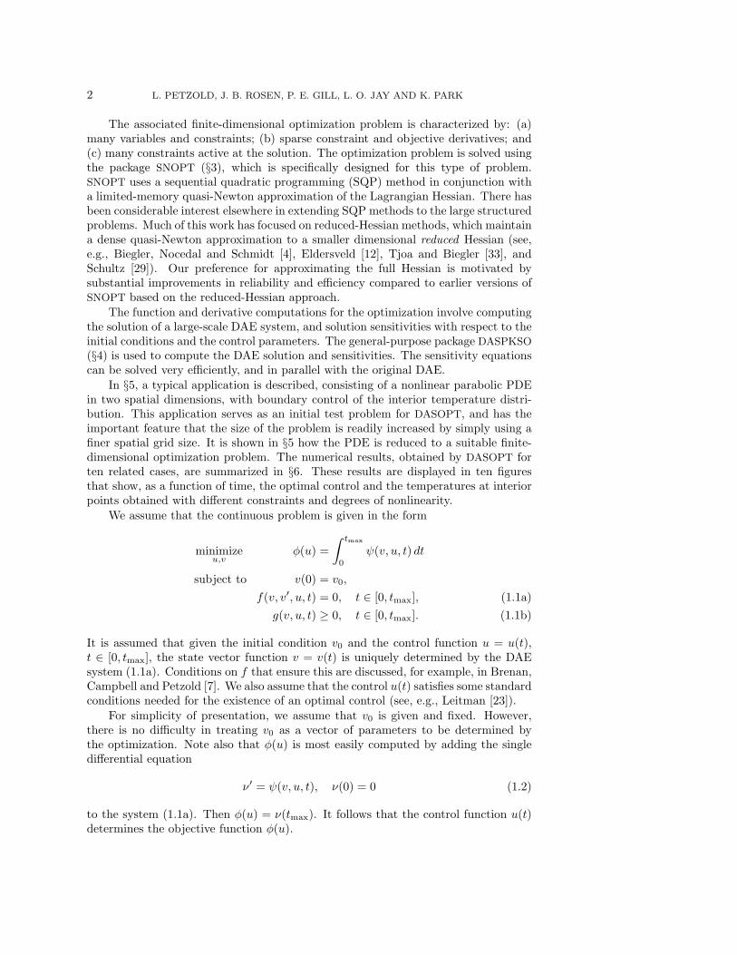
5. Formulation of a PDE test problem. In order to test DASOPT on a real-istic model problem, we formulated a boundary control heating problem in two spatialdimensions. This model problem is described by a nonlinear parabolic PDE. It is atwo-dimensional generalization of the model problem described in [22]. A rectangu-lar domain in space is heated by controlling the temperature on its boundaries. Itis desired that the transient temperature in a specified interior subdomain follow aprescribed temperature-time trajectory as closely as possible. The domain Ω is givenby

Ω = (x, y) | 0 ≤ x ≤ xmax, 0 ≤ y ≤ ymax,

and the control boundaries are given by

∂Ω1 = (x, y) | y = 0, and ∂Ω2 = (x, y) | x = 0.

The temperature distribution in Ω, as a function of time, is controlled by the energyinput across the boundaries ∂Ω1 and ∂Ω2, as discussed below. The other two bound-aries (x = xmax and y = ymax) are assumed to be insulated, so that no energy flowsinto or out of Ω along the normals to these boundaries. The temperature must becontrolled in the subdomain

Ωc = (x, y) | xc ≤ x ≤ xmax, yc ≤ y ≤ ymax.

This is illustrated in Fig. 5.1.The control problem is to be solved for the time interval t ∈ [0, tmax]. The

temperature T = T (x, y, t) is then determined by the nonlinear parabolic PDE givenbelow, for (x, y, t) ∈ Ω × [0, tmax].

The temperature T is controlled by heat sources located on the boundaries ∂Ω1

and ∂Ω2. These heat sources are represented by control functions u1(x, t) on ∂Ω1,and u2(y, t) on ∂Ω2. The control functions are to be determined. The objective is tocontrol the temperature-time trajectory on the subdomain Ωc. A target trajectory


T = 0y

T = 0x

x

y

y

y

0 x x

max

maxc

c

Ω

Ω

∂

∂Ω

Ω

1

2

c

Fig. 5.1. Two dimensional spatial domain for the parabolic control test problem.

τ(t), t ∈ [0, tmax], is specified. The actual temperature in Ωc should approximate τ(t)as closely as possible.

We measure the difference between T (x, y, t) and τ(t) on Ωc by the function

φ(u) =

∫ tmax

0

∫ ymax

yc

∫ xmax

xc

w(x, y, t)[T (x, y, t) − τ(t)]2 dx dy dt, (5.1)

where w(x, y, t) ≥ 0 is a specified weighting function. The control functions u1 andu2 are determined so as to

minimizeu

φ(u), (5.2)

subject to T (x, y, t) satisfying the PDE and other constraints.The temperature T (x, y, t) must satisfy the following PDE, boundary conditions,

and bounds

α(T )[Txx + Tyy] + S(T ) = Tt, (x, y, t) ∈ Ω × [0, tmax]

T (x, 0, t) − λTy = u1(x, t), x ∈ ∂Ω1

T (0, y, t) − λTx = u2(y, t), y ∈ ∂Ω2

Tx(xmax, y, t) = 0,

Ty(x, ymax, t) = 0,

0 ≤ T (x, y, t) ≤ Tmax.

(5.3)

The controls u1 and u2 are also required to satisfy the bounds

0 ≤ u1, u2 ≤ umax.

The initial temperature distribution T (x, y, 0) is a specified function. The coefficientα(T ) = λ/c(T ), where λ is the heat conduction coefficient and c(T ) is the heatcapacity. The source term S(T ) represents internal heat generation, and is given by

S(T ) = Smaxe−β1/(β2+T )

where Smax, β1, β2 ≥ 0 are specified nonnegative constants.


The numerical solution has been obtained by constructing finite-difference grids inspace, and solving the resulting ODEs by the multiple-shooting method as describedbelow.

A uniform rectangular grid is constructed on the domain Ω

xi = i∆x, i = 0, 1, . . . ,m, ∆x = xmax/m

yj = j∆y, j = 0, 1, . . . , n, ∆y = ymax/n.

Then let

Tij(t) = T (xi, yj , t), u1i(t) = u1(xi, t), αij(t) = α(Tij(t)),

Sij(t) = S(Tij(t)), u2j(t) = u2(yj , t).

The PDE is then approximated in the interior of Ω by the following system of(m− 1)(n− 1) ODEs

dTij

dt=

αij

∆x2[Ti−1,j − 2Tij + Ti+1,j ]

+αij

∆y2[Ti,j−1 − 2Tij + Ti,j+1] + Sij ,

(5.4)

for i = 1, 2, . . . ,m− 1, j = 1, 2, . . . , n− 1. Each of the 2(m+ n) boundary points alsosatisfies a differential equation similar to (5.4). These will include values outside Ω,which are eliminated by using the boundary conditions. Specifically, we use

Ti,n+1 = Ti,n−1, i = 0, 1, . . . ,m

Tm+1,j = Tm−1,j j = 0, 1, . . . , n,

to approximate the conditions Ty = 0 and Tx = 0.The finite-difference approximations to the boundary conditions on ∂Ω1 and ∂Ω2

are given by

Ti0 −λ

2∆y(Ti1 − Ti,−1) = u1i, i = 0, 1, . . . ,m (5.5a)

T0j −λ

2∆x(T1j − T−1,j) = u2j , j = 0, 1, . . . , n (5.5b)

These relations are used to eliminate the values Ti,−1 and T−1,j from the differentialequations (as in (5.4)), for the functions Tij on ∂Ω1 and ∂Ω2. As a result, the controlfunctions u1i and u2j are explicitly included in these differential equations, giving2(m + n) additional differential equations. Together with the (m − 1)(n − 1) ODEsgiven by (5.4), this gives a total of (m + 1)(n + 1) ODEs for the same number ofunknown functions Tij(t). To simplify the notation in what follows, this system of(m+ 1)(n+ 1) ODEs will be represented by

dv(t)

dt= f(v, u(t), t), v(0) = v0, (5.6)

where v0 represents the initial value of v(t), and u = u(t) the control functions. Thevector function u(t) has elements u1i(t), i = 0, 1, . . . ,m, and u2j(t), j = 0, 1, . . . , n.These ODEs correspond to those given by (1.1a).

As discussed earlier the multiple shooting method is applied by dividing the totaltime interval [0, tmax] into N equal lengths ∆t, with N∆t = tmax. Also let tk = k∆t,


k = 0, 1, . . . , N . The system of ODEs (5.6) on [0, tmax] is now considered as Nindependent systems, each on its own time subinterval [tk, tk+1]. Let vk(t) representv(t) and uk(t) represent u(t) on [tk, tk+1], and vk be the initial value of vk(t). Thenvk(t) must satisfy

dvk

dt= f(vk, uk(t), t), vk(tk) = vk, k = 0, 1, . . . , N − 1.

The value of v0 = v0, while the remaining initial values vk, k = 1, 2, . . . , N − 1,are determined by continuity conditions (2.6) in the optimization problem. This isillustrated in Fig. 5.2.

t

y

x

t

t 0

1

k

k+1t

t = t N max

T = 0

T = 0

y

x

y

x

max

max

ΩΩ

Ω

∂

∂ 1

2

t

= 0

v

vu

k+1

k

k

Fig. 5.2. Space-time domain for test problem showing the shooting intervals.

For each subinterval, the control vector uk(t) is approximated as in (2.3), withthe parameters uk being determined by the optimization. Bounds on the uk(t) att = tk (and any additional points) give linear inequalities on the ukl. Since uk(t) isgiven in terms of the control parameters uk, it is clear that vk(tk+1) is a function ofvk and uk. This dependence has been explicitly given earlier in (2.5).

Equations (2.6) represent the N(m + 1)(n + 1) individual equality constraintsthat must be satisfied. The optimization code SNOPT requires the Jacobian of theseconstraints with respect to the parameters vk and uk. These partial derivatives canbe obtained using the sensitivity capability of DASPKSO. The sensitivity of eachelement of s(vk, uk) with respect to each element of vk and uk must be computed.As s, vk ∈ IRnv and uk ∈ IRnu , this requires that for each subinterval, nv(nv + nu)sensitivity calculations are required. Thus a total of Nnv(nv + nu) such calculationsmust be made to estimate the Jacobian. In order to reduce this computation to areasonable size, other approaches are needed, and they are being investigated.

The objective function is computed by adding the single ODE (1.2) to the system(5.6). The gradient of the objective function is then obtained as part of the sensitivitycomputation.

The state bounds on the Tij(tk) are imposed at each discrete time tk by the simplebounds

0 ≤ vk ≤ Tmaxe, k = 1, 2, . . . , N. (5.7)

These will enforce the bounds at the points tk, but there may be some small violationat intermediate time points.


The optimization problem to be solved can now be stated as follows: minimizethe spatial discretization of (5.1) subject to the linear equality constraints (2.4), thebound constraints (5.7), and the nonlinear equality constraints (2.6).

The nonlinear parabolic PDE boundary control problem described by (5.1), (5.2)and (5.3) has been solved computationally using the discrete approximation describedabove. Numerical results for ten cases, including cases with the nonlinear source termand bounds on the interior temperatures, are summarized in the next section.

6. Computational results with DASOPT. The purpose of the computationssummarized in this section was to test the DASOPT code on the relatively simple 2Dnonlinear parabolic PDE problem described in the previous section. This test problemhas the property that the size of the optimization problem can be easily increased bysimply using a finer spatial grid. This readily permits the dependence of solution timeon problem size to be observed.

It was also important to determine if the combination of DASPKSO and SNOPT

would result in a convergent algorithm for this type of problem. As shown in theexamples below, convergence to an optimal control was typically obtained in no morethan 17 major iterations of SNOPT. While this parabolic PDE can be solved usingsingle shooting, we used multiple shooting in order to test the performance of thecombined system.

This type of problem also permitted testing the capability to impose inequalityconstraints on the state variables, in this case bounds on the interior temperatures.This ability is clearly shown by comparing the control and temperatures obtainedwith and without bounds on the maximum permitted interior temperatures.

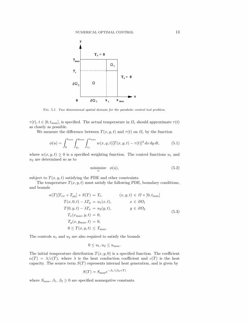
The computational results obtained with DASOPT, using the CRAY C90, onthe optimal control 2D nonlinear PDE will now be summarized. The rectangulardomain (see Fig. 5.1) is chosen as Ω = (x, y) | 0 ≤ x ≤ 0.8, 0 ≤ y ≤ 1.6. Thetime integration interval is [0, 2] and the goal is to follow as closely as possible aspecified time-temperature trajectory τ(t) (as specified in all following figures) in thesubdomain Ωc = (x, y) | 0.6 ≤ x ≤ 0.8, 1.2 ≤ y ≤ 1.6. We want to determinethe boundary control so as to minimize the objective (5.1) with w(x, y, t) = 0 fort ∈ [0, 0.2] and w(x, y, t) = 1 for t ∈ [0.2, 2]. On the boundaries ∂Ω1 and ∂Ω2 thecontrols u1(x, t) and u2(y, t) are given by a control function u(t) as follows:

u1(x, t) =

u(t) 0 ≤ x ≤ 0.2;(

1 −x− 0.2

1.2

)u(t) 0.2 ≤ x ≤ 0.8.

u2(x, t) =

u(t) 0 ≤ y ≤ 0.4;(

1 −y − 0.4

2.4

)u(t) 0.4 ≤ y ≤ 1.6.

(6.1)

Note that for any fixed t, u is constant on the boundary ∂Ω1 for 0 ≤ x ≤ 0.2, andthen decreases linearly to u/2 at x = 0.8. The control u2 on ∂Ω2 is similar. We alsoimpose the initial condition u(0) = 0.

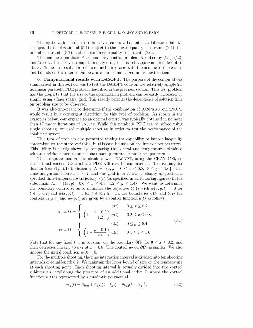
For the multiple shooting, the time integration interval is divided into ten shootingintervals of equal length 0.2. We maintain the lower bound of zero on the temperatureat each shooting point. Each shooting interval is actually divided into two controlsubintervals (explaining the presence of an additional index j) where the controlfunction u(t) is represented by a quadratic polynomial

ukj(t) = ukj0 + ukj1(t− tkj) + ukj2(t− tkj)2. (6.2)


We enforce continuity in time at the extremities of each control subinterval amongall ukj(t) and their derivative u′kj(t). We also impose the following bounds on thecontrol parameters

|ukj1| ≤ 5, |ukj2| ≤ 7.

We maintain an upper bound on the maximal value of the control umax = 1.1 and,except in one case, a lower bound of zero at the extremities and in the middle of eachcontrol subinterval.

In all ten test cases presented here, the PDE parameters λ, c and α were assumedto be constant, with the values λ = c = 1

2 , and α = 1. Therefore, the PDE is linearwhen Smax = 0. The parameters in S(T ) were chosen as β1 = 0.2 and β2 = 0.05.In addition to the linear case Smax = 0, the values of Smax = 0.5, 1.0, were used toshow the significant effect of the nonlinear heat source term. At t = 0, the initialtemperature Tij(0) = 0 was used for all cases.

The effect of the state variable bounds is shown by requiring that the temperaturesat every space-time grid-point satisfy Tij(tk) ≤ Tmax. This upper bound was imposedin three of the ten cases. A lower bound of zero was also imposed for all ten cases,but was only active in Case 9.

The computational results obtained for the ten cases are summarized in Table 6.1.The time dependent optimal solution for each of the ten cases is presented in Figs. 6.1–6.10. The figure number corresponds to the case number in Table 6.1, so that Fig. 6.xshows results for Case x.

Table 6.1

Summary of test problem optimal solutions.

Case Grid Smax Tmax Initial φ Major Time TimeSize Bound Values (×105) Itns (Secs) /Itn

1 5× 5 0.0 None 0 1.525 17 176 10.42 5× 9 0.0 None 0 1.517 16 488 30.53 5× 17 0.0 None 0 1.515 16 1584 99.04 9× 17 0.0 None 0 1.536 11 3489 317.25 5× 9 0.5 None #2 1.836 16 432 27.06 5× 9 1.0 None #5 15.92 7 208 29.77 5× 9 0.0 0.7 0 5.754 9 285 31.78 5× 9 0.5 0.7 #7 2.490 7 224 32.09 5× 9 1.0 0.7 #5 4.277 6 204 34.0

10 5× 9 0.0 None 0 0.826 17 545 32.1

In Table 6.1, the grid size describes the discrete grid on the spatial domain Ω.For example, the 5 × 5 grid gives ∆x = 0.2, ∆y = 0.4, and defines Tij , for i, j = 0, 1,2, 3, 4. Thus for an m× n grid, there are mn spatial grid points, including boundarygrid points.

The column “Smax” shows the degree of nonlinearity of the problem, whereSmax = 0 implies that the problem is linear. The column “Tmax Bound” shows whena state upper bound is imposed. The column “Initial Values” gives the initial esti-mates used for the Tij(tk) and the ukj control coefficients. The value zero assumes noknowledge of the optimal solution and gives the most difficult optimization problem.Much better estimates can be obtained from the optimal solution with a coarser grid,or a lower value of Smax. A nonzero entry indicates that the optimal Tij(tk) and ukj


from a previous case were used as initial estimates. The value of the entry gives theparticular case used.

The SNOPT default parameter settings were used throughout, except for theoptimality tolerance, which was set to 10−5. Roughly speaking, these settings give anapproximate minimizer with a reduced-gradient norm less than 10−5 and a maximumnonlinear constraint violation less than 10−6 (for further details of the terminationcriteria, see [25]). The default maximum number of limited memory updates stored(the number “ℓ” of §3) is 20.

The last four columns in Table 6.1 give the results of the computation. Theminimum value of the objective function φ, scaled by 105, is shown for each case. Thenumber of major iterations required by SNOPT, the CRAY C90 cpu time (in seconds),and the average time per iteration are given in the last three columns.

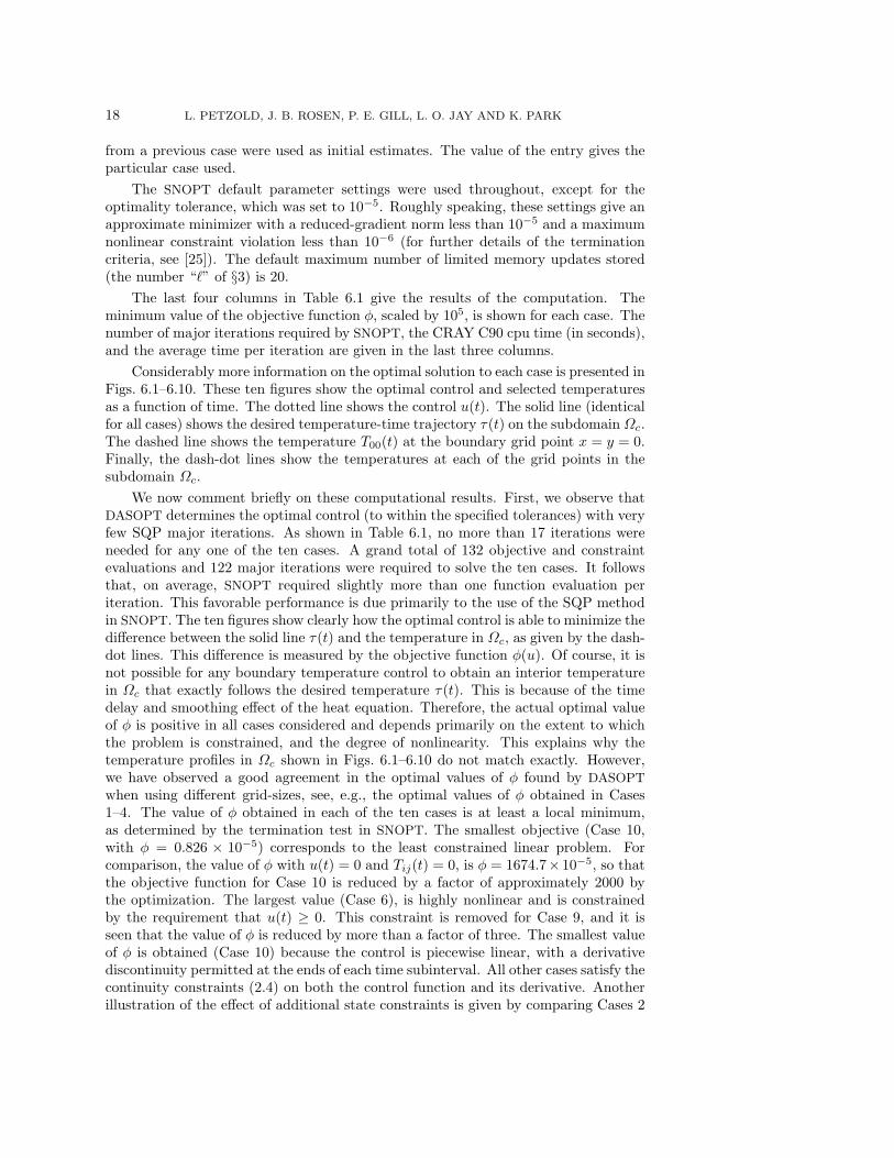
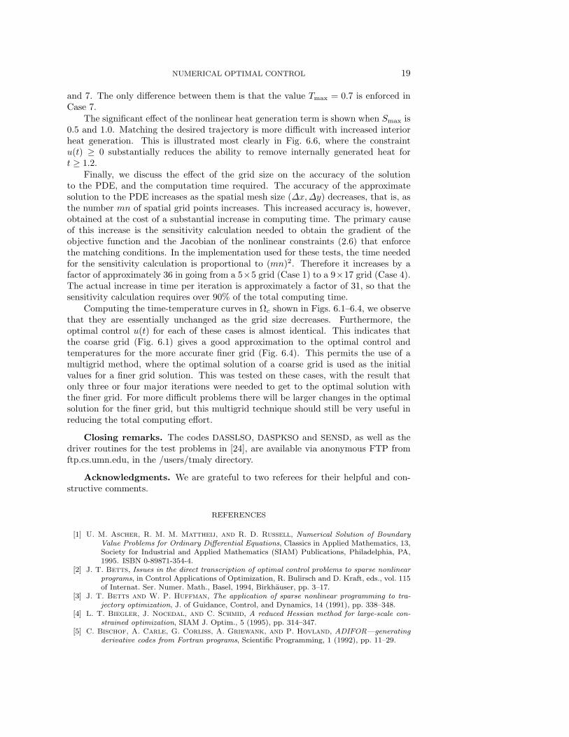
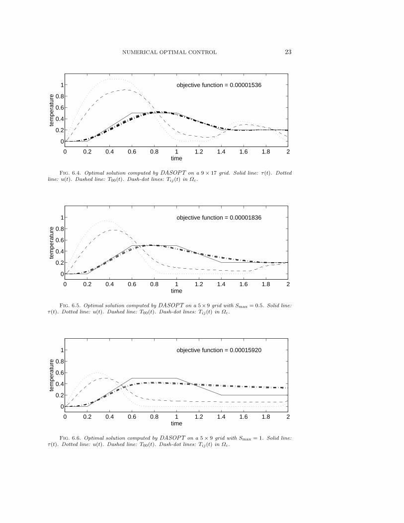
Considerably more information on the optimal solution to each case is presented inFigs. 6.1–6.10. These ten figures show the optimal control and selected temperaturesas a function of time. The dotted line shows the control u(t). The solid line (identicalfor all cases) shows the desired temperature-time trajectory τ(t) on the subdomain Ωc.The dashed line shows the temperature T00(t) at the boundary grid point x = y = 0.Finally, the dash-dot lines show the temperatures at each of the grid points in thesubdomain Ωc.

We now comment briefly on these computational results. First, we observe thatDASOPT determines the optimal control (to within the specified tolerances) with veryfew SQP major iterations. As shown in Table 6.1, no more than 17 iterations wereneeded for any one of the ten cases. A grand total of 132 objective and constraintevaluations and 122 major iterations were required to solve the ten cases. It followsthat, on average, SNOPT required slightly more than one function evaluation periteration. This favorable performance is due primarily to the use of the SQP methodin SNOPT. The ten figures show clearly how the optimal control is able to minimize thedifference between the solid line τ(t) and the temperature in Ωc, as given by the dash-dot lines. This difference is measured by the objective function φ(u). Of course, it isnot possible for any boundary temperature control to obtain an interior temperaturein Ωc that exactly follows the desired temperature τ(t). This is because of the timedelay and smoothing effect of the heat equation. Therefore, the actual optimal valueof φ is positive in all cases considered and depends primarily on the extent to whichthe problem is constrained, and the degree of nonlinearity. This explains why thetemperature profiles in Ωc shown in Figs. 6.1–6.10 do not match exactly. However,we have observed a good agreement in the optimal values of φ found by DASOPT

when using different grid-sizes, see, e.g., the optimal values of φ obtained in Cases1–4. The value of φ obtained in each of the ten cases is at least a local minimum,as determined by the termination test in SNOPT. The smallest objective (Case 10,with φ = 0.826 × 10−5) corresponds to the least constrained linear problem. Forcomparison, the value of φ with u(t) = 0 and Tij(t) = 0, is φ = 1674.7× 10−5, so thatthe objective function for Case 10 is reduced by a factor of approximately 2000 bythe optimization. The largest value (Case 6), is highly nonlinear and is constrainedby the requirement that u(t) ≥ 0. This constraint is removed for Case 9, and it isseen that the value of φ is reduced by more than a factor of three. The smallest valueof φ is obtained (Case 10) because the control is piecewise linear, with a derivativediscontinuity permitted at the ends of each time subinterval. All other cases satisfy thecontinuity constraints (2.4) on both the control function and its derivative. Anotherillustration of the effect of additional state constraints is given by comparing Cases 2


and 7. The only difference between them is that the value Tmax = 0.7 is enforced inCase 7.

The significant effect of the nonlinear heat generation term is shown when Smax is0.5 and 1.0. Matching the desired trajectory is more difficult with increased interiorheat generation. This is illustrated most clearly in Fig. 6.6, where the constraintu(t) ≥ 0 substantially reduces the ability to remove internally generated heat fort ≥ 1.2.

Finally, we discuss the effect of the grid size on the accuracy of the solutionto the PDE, and the computation time required. The accuracy of the approximatesolution to the PDE increases as the spatial mesh size (∆x,∆y) decreases, that is, asthe number mn of spatial grid points increases. This increased accuracy is, however,obtained at the cost of a substantial increase in computing time. The primary causeof this increase is the sensitivity calculation needed to obtain the gradient of theobjective function and the Jacobian of the nonlinear constraints (2.6) that enforcethe matching conditions. In the implementation used for these tests, the time neededfor the sensitivity calculation is proportional to (mn)2. Therefore it increases by afactor of approximately 36 in going from a 5×5 grid (Case 1) to a 9×17 grid (Case 4).The actual increase in time per iteration is approximately a factor of 31, so that thesensitivity calculation requires over 90% of the total computing time.

Computing the time-temperature curves in Ωc shown in Figs. 6.1–6.4, we observethat they are essentially unchanged as the grid size decreases. Furthermore, theoptimal control u(t) for each of these cases is almost identical. This indicates thatthe coarse grid (Fig. 6.1) gives a good approximation to the optimal control andtemperatures for the more accurate finer grid (Fig. 6.4). This permits the use of amultigrid method, where the optimal solution of a coarse grid is used as the initialvalues for a finer grid solution. This was tested on these cases, with the result thatonly three or four major iterations were needed to get to the optimal solution withthe finer grid. For more difficult problems there will be larger changes in the optimalsolution for the finer grid, but this multigrid technique should still be very useful inreducing the total computing effort.

Closing remarks. The codes DASSLSO, DASPKSO and SENSD, as well as thedriver routines for the test problems in [24], are available via anonymous FTP fromftp.cs.umn.edu, in the /users/tmaly directory.

Acknowledgments. We are grateful to two referees for their helpful and con-structive comments.

REFERENCES

[1] U. M. Ascher, R. M. M. Mattheij, and R. D. Russell, Numerical Solution of Boundary

Value Problems for Ordinary Differential Equations, Classics in Applied Mathematics, 13,Society for Industrial and Applied Mathematics (SIAM) Publications, Philadelphia, PA,1995. ISBN 0-89871-354-4.

[2] J. T. Betts, Issues in the direct transcription of optimal control problems to sparse nonlinear

programs, in Control Applications of Optimization, R. Bulirsch and D. Kraft, eds., vol. 115of Internat. Ser. Numer. Math., Basel, 1994, Birkhauser, pp. 3–17.

[3] J. T. Betts and W. P. Huffman, The application of sparse nonlinear programming to tra-

jectory optimization, J. of Guidance, Control, and Dynamics, 14 (1991), pp. 338–348.[4] L. T. Biegler, J. Nocedal, and C. Schmid, A reduced Hessian method for large-scale con-

strained optimization, SIAM J. Optim., 5 (1995), pp. 314–347.[5] C. Bischof, A. Carle, G. Corliss, A. Griewank, and P. Hovland, ADIFOR—generating

derivative codes from Fortran programs, Scientific Programming, 1 (1992), pp. 11–29.


[6] K. E. Brenan, Differential-algebraic equations issues in the direct transcription of path con-

strained optimal control problems, Ann. Numer. Math., 1 (1994), pp. 247–263.[7] K. E. Brenan, S. L. Campbell, and L. R. Petzold, Numerical Solution of Initial-Value Prob-

lems in Differential-Algebraic Equations, SIAM Publications, Philadelphia, second ed.,1995. ISBN 0-89871-353-6.

[8] A. Buckley and A. LeNir, QN-like variable storage conjugate gradients, Math. Prog., 27(1983), pp. 155–175.

[9] R. Bulirsch, E. Nerz, H. J. Pesch, and O. von Stryk, Combining direct and indirect

methods in optimal control: Range maximization of a hang glider, in Calculus of Variations,Optimal Control Theory and Numerical Methods., R. Bulirsch, A. Miele, J. Stoer, andK. H. Well, eds., vol. 111 of Internat. Ser. Numer. Math., Basel, 1993, Birkhauser, pp. 273–288.

[10] M. Caracotsios and W. E. Stewart, Sensitivity analysis of initial value problems with mixed

ODEs and algebraic equations, Computers and Chemical Engineering, 9 (1985), pp. 359–365.

[11] E. D. Dickmanns and K. H. Well, Approximate solution of optimal control problems using

third-order Hermite polynomial functions, in Proc. 6th Technical Conference on Optimiza-tion Techniques, Berlin, Heidelberg, New York, London, Paris and Tokyo, 1975, SpringerVerlag.

[12] S. K. Eldersveld, Large-scale sequential quadratic programming algorithms, PhD thesis, De-partment of Operations Research, Stanford University, Stanford, CA, 1991.

[13] J. C. Gilbert and C. Lemarechal, Some numerical experiments with variable-storage quasi-

Newton algorithms, Math. Prog., (1989), pp. 407–435.[14] P. E. Gill and W. Murray, Conjugate-gradient methods for large-scale nonlinear optimiza-

tion, Report SOL 79-15, Department of Operations Research, Stanford University, Stan-ford, CA, 1979.

[15] P. E. Gill, W. Murray, and M. A. Saunders, SNOPT: An SQP algorithm for large-scale

constrained optimization, Numerical Analysis Report 96-2, Department of Mathematics,University of California, San Diego, La Jolla, CA, 1996.

[16] P. E. Gill, W. Murray, M. A. Saunders, and M. H. Wright, Maintaining LU factors of a

general sparse matrix, Linear Algebra and its Applications, 88/89 (1987), pp. 239–270.[17] P. E. Gill, W. Murray, and M. H. Wright, Practical Optimization, Academic Press, London

and New York, 1981. ISBN 0-12-283952-8.[18] D. M. Gritsis, C. C. Pantelides, and R. W. H. Sargent, Optimal control of systems de-

scribed by index two differential-algebraic equations, SIAM J. Sci. Comput., 16 (1995),pp. 1349–1366.

[19] C. R. Hargraves and S. W. Paris, Direct trajectory optimization using nonlinear program-

ming and collocation, J. of Guidance, Control, and Dynamics, 10 (1987), pp. 338–348.[20] D. Kraft, On converting optimal control problems into nonlinear programming problems,

in Computational Mathematical Programming, K. Schittkowski, ed., NATO ASI Series F:Computer and Systems Sciences 15, Springer Verlag, Berlin and Heidelberg, 1985, pp. 261–280.

[21] R. Lamour, A well posed shooting method for transferable DAEs, Numer. Math., 59 (1991),pp. 815–829.

[22] F. Leibfritz and E. W. Sachs, Numerical solution of parabolic state constrained control

problems using SQP and interior point methods, in Large Scale Optimization: the Stateof the Art, W. W. Hager, D. W. Hearn, and P. M. Pardalos, eds., Kluwer AcademicPublishers, Dordrecht, 1994, pp. 245–258. ISBN 0-7923-2798-5.

[23] G. Leitmann, The Calculus of Variations and Optimal Control, Mathematical Concepts andMethods in Science and Engineering, 24, Plenum Press, New York and London, 1981. ISBN0-306-40707-8.

[24] T. Maly and L. R. Petzold, Numerical methods and software for sensitivity analysis of

differential-algebraic systems. to appear in Applied Numerical Mathematics, 1996.[25] B. A. Murtagh and M. A. Saunders, MINOS 5.4 User’s Guide, Report SOL 83-20R, De-

partment of Operations Research, Stanford University, Stanford, CA, 1993.[26] J. Nocedal, Updating quasi-Newton matrices with limited storage, Math. Comput., 35 (1980),

pp. 773–782.[27] C. C. Pantelides, R. W. H. Sargent, and V. S. Vassiliadis, Optimal control of multi-

stage systems described by high-index differential-algebraic equations, Internat. Ser. Nu-mer. Math., 115 (1994), pp. 177–191.

[28] H. J. Pesch, Real-time computation of feedback controls for constrained optimal control prob-

lems, Optimal Control Appl. Methods, 10 (1989), pp. 129–171.


[29] V. H. Schultz, Reduced SQP methods for large-scale optimal control problems in DAE with

application to path planning problems for satellite mounted robots, PhD thesis, Universityof Heidelberg, 1996.

[30] V. H. Schulz, H.-G. Bock, and M. C. Steinbach, Exploiting invariants in the numerical

solution of multipoint boundary value problems for DAE. submitted to SIAM J. Sci.Comput., 1996.

[31] M. C. Steinbach, A structured interior point SQP method for nonlinear optimal control prob-

lems, in Control Applications of Optimization, R. Bulirsch and D. Kraft, eds., vol. 115 ofInternat. Ser. Numer. Math., Basel, 1994, Birkhauser, pp. 213–222.

[32] P. Tanartkit and L. T. Biegler, Stable decomposition for dynamic optimization, Ind. Eng.Chem. Res., (1995), pp. 1253–1266.

[33] I.-B. Tjoa and L. T. Biegler, A reduced SQP strategy for errors-in-variables estimation,Comput. Chem. Eng., 16 (1992), pp. 523–533.

[34] O. von Stryk, Numerical solution of optimal control problems by direct collocation, in ControlApplications of Optimization, R. Bulirsch, A. Miele, J. Stoer, and K. H. Well, eds., vol. 111of Internat. Ser. Numer. Math., Basel, 1993, Birkhauser, pp. 129–143.

[35] O. von Stryk and R. Bulirsch, Direct and indirect methods for trajectory optimization, Ann.Oper. Res., 37 (1992), pp. 357–373.


0 0.2 0.4 0.6 0.8 1 1.2 1.4 1.6 1.8 2

0

0.2

0.4

0.6

0.8

1

time

tem

pera

ture

objective function = 0.00001525

Fig. 6.1. Optimal solution computed by DASOPT on a 5 × 5 grid. Solid line: τ(t). Dotted

line: u(t). Dashed line: T00(t). Dash-dot lines: Tij(t) in Ωc.

0 0.2 0.4 0.6 0.8 1 1.2 1.4 1.6 1.8 2

0

0.2

0.4

0.6

0.8

1

time

tem

pera

ture




0 0.2 0.4 0.6 0.8 1 1.2 1.4 1.6 1.8 2

0

0.2

0.4

0.6

0.8

1

time

tem

pera

ture





0 0.2 0.4 0.6 0.8 1 1.2 1.4 1.6 1.8 2

0

0.2

0.4

0.6

0.8

1

time

tem

pera

ture




0 0.2 0.4 0.6 0.8 1 1.2 1.4 1.6 1.8 2

0

0.2

0.4

0.6

0.8

1

time

tem

pera

ture


Fig. 6.5. Optimal solution computed by DASOPT on a 5× 9 grid with Smax = 0.5. Solid line:

τ(t). Dotted line: u(t). Dashed line: T00(t). Dash-dot lines: Tij(t) in Ωc.

0 0.2 0.4 0.6 0.8 1 1.2 1.4 1.6 1.8 2

0

0.2

0.4

0.6

0.8

1

time

tem

pera

ture


Fig. 6.6. Optimal solution computed by DASOPT on a 5 × 9 grid with Smax = 1. Solid line:



0 0.2 0.4 0.6 0.8 1 1.2 1.4 1.6 1.8 2

0

0.2

0.4

0.6

0.8

1

time

tem

pera

ture


Fig. 6.7. Optimal solution computed by DASOPT on a 5×9 grid with Tij(t) ≤ 0.7. Solid line:


0 0.2 0.4 0.6 0.8 1 1.2 1.4 1.6 1.8 2

0

0.2

0.4

0.6

0.8

1

time

tem

pera

ture


Fig. 6.8. Optimal solution computed by DASOPT on a 5 × 9 grid with Tij(t) ≤ 0.7 and

Smax = 0.5. Solid line: τ(t). Dotted line: u(t). Dashed line: T00(t). Dash-dot lines: Tij(t) in Ωc.

0 0.2 0.4 0.6 0.8 1 1.2 1.4 1.6 1.8 2-0.2

0

0.2

0.4

0.6

0.8

1

time

tem

pera

ture


Fig. 6.9. Optimal solution computed by DASOPT on a 5×9 grid with Tij(t) ≤ 0.7, Smax = 1,and no lower bound on u(t). Solid line: τ(t). Dotted line: u(t). Dashed line: T00(t). Dash-dot

lines: Tij(t) in Ωc.


0 0.2 0.4 0.6 0.8 1 1.2 1.4 1.6 1.8 2

0

0.2

0.4

0.6

0.8

1

time

tem

pera

ture


Fig. 6.10. Optimal solution computed by DASOPT on a 5 × 9 grid with piecewise continuous

linear control u(t). Solid line: τ(t). Dotted line: u(t). Dashed line: T00(t). Dash-dot lines: Tij(t)in Ωc.

numerical optimal control of parabolic …peg/papers/dasopt.pdfnumerical optimal control of...

Documents