numerical of lubrication

NUMERICALCALCULATIONOF LUBRICATION

NUMERICALCALCULATIONOF LUBRICATIONMETHODS AND PROGRAMS

Ping Huang

South China University of Technology, Guangzhou, China

This ed ition first published 2013

# 2013 Tsinghua University Press. All rights re served.

Published by John Wiley & Sons Singapore Pte. Ltd., 1 Fusionopolis Walk, #07-01 Solaris South Tower, Singapore 138628,

under exclusive license by Tsinghua University Press in all medi a throughout the world excluding Mainland China and

excluding Simpli fied and Traditional Chinese lan guages.

For details of our global edi torial offices, for customer services and for information about how to apply for permi ssion to

reuse th e copyright material in this book please see our website at www.wiley.com.

All Rights Reserved. No part of this publication may be reproduced, stored in a retrieval system or transmitted, in any

form or by any means, electronic, mechanical, photocopying, recording, scanning, or otherwise, except as expressly

permitted by law, without either the prior written permi ssion of the Publisher, or authoriz ation through payment of the

appropriate photoc opy fee to the Copyright Cl earance Cente r. Requests for perm ission should be addressed to the Publisher,

John Wiley & Sons Singapore Pte. Ltd., 1 Fusionopolis Walk, #07-01 Solaris South Tower, Singapore 138628,

tel: 65-66438000 , fax: 65-66438008 , email: [email protected].

Wiley also publishes its books in a variety of electronic formats. Some content that appears in print may not be available in

electronic books.

Designations used by companies to distinguish their products are often claimed as trademarks. All brand names and

product names used in this book are trade names, service marks, trademarks or registered trademarks of their respective

owners. The Publisher is not associated with any product or vendor mentioned in this book. This publication is designed to

provide accurate and authoritative information in regard to the subject matter covered. It is sold on the understanding that

the Publisher is not engaged in rendering professional services. If professional advice or other expert assistance is required,

the services of a competent professional should be sought.

Limit of Liability/Disclaimer of Warranty: While the publisher and author have used their best efforts in preparing this

book, they make no representations or warranties with respect to the accuracy or completeness of the contents of this book

and specifically disclaim any implied warranties of merchantability or fitness for a particular purpose. It is sold on the

understanding that the publisher is not engaged in rendering professional services and neither the publisher nor the author

shall be liable for damages arising herefrom. If professional advice or other expert assistance is required, the services of a

competent professional should be sought.

Library of Congress Cataloging-in-Publication Data

Huang, Ping, 1957-

Numerical calculation of lubrication : methods and programs / Huang Ping.

pages cm

Includes bibliographical references and index.

ISBN 978-1-118-45119-9 (cloth)

1. Lubrication and lubricants—Mathematical models. I. Title.

TJ1077.H92 2013

621.8 09—dc23

2013014001

Set in 11/13 pt Times by Thomson Digital, Noida, India

1/2013

www.wiley.com

mailto:[email protected]

Contents

Preface xv

Part 1 NUMERICAL METHOD FOR REYNOLDS EQUATION 1

1 Reynolds Equation and its Discrete Form 31.1 General Reynolds Equation and Its Boundary Conditions 3

1.1.1 Reynolds Equation 3

1.1.2 Definite Condition 3

1.1.3 Computation of Lubrication Performances 5

1.2 Reynolds Equations for Some Special Working Conditions 6

1.2.1 Slider and Thrust Bearing 6

1.2.2 Journal Bearing 7

1.2.3 Hydrostatic Lubrication 8

1.2.4 Squeeze Bearing 9

1.2.5 Dynamic Bearing 9

1.2.6 Gas Bearing 10

1.3 Finite Difference Method of Reynolds Equation 10

1.3.1 Discretization of Equation 11

1.3.2 Difference Form of Reynolds Equation 12

1.3.3 Iteration of Differential Equation 13

1.3.4 Iteration Convergence Condition 13

2 Numerical Method and Program for Incompressible and SteadyLubrication of One-dimensional Slider 172.1 Basic Equations 17


2.1.2 Boundary Conditions 18

2.1.3 Continuity Equation 18

2.2 Numerical Method for Incompressible and Steady Lubrication

of One-dimensional Slider 18

2.2.1 Discrete Reynolds Equation 19

2.3 Calculation Program for Incompressible and Steady Lubrication

of One-dimensional Slider 20

2.3.1 Introduction 20

2.3.2 Calculation Diagram 21

2.3.3 Calculation Program 21

2.3.4 Calculation Results 24

3 Numerical Method and Program for Incompressible and SteadyLubrication of Two-dimensional Slider 253.1 Basic Equations 25

3.2 Discrete Reynolds Equation 26


of Two-dimensional Slider 27





4 Numerical Method and Program for Incompressible and SteadyLubrication of Journal Bearing 334.1 Basic Equations 33

4.1.1 Axis Position and Clearance Shape 33


4.2 Numerical Method for Incompressible and Steady Lubrication

of Journal Bearing 35

4.2.1 Dimensionless Reynolds Equation 35

4.2.2 Discrete Form of Reynolds Equation 36


of Journal Bearing 37




5 Numerical Method and Program for IncompressibleSqueeze Lubrication 415.1 Basic Equation 41

5.2 Numerical Method and Program for Rectangular Plane Squeeze 42

5.2.1 Basic Equations 42

5.2.2 Numerical Method 42




vi Contents

5.3 Numerical Method and Program for Disc Squeeze 47






5.4 Numerical Method and Program for Journal Bearing Squeeze 52






6 Numerical Method and Program for Dynamic Bearing 616.1 Basic Equations 61

6.2 Numerical Method for Trace of Journal Center 65


6.2.2 Calculation Steps 66

6.3 Calculation Program for Dynamic Journal Bearing 67





7 Numerical Method and Program for Gas Lubrication 857.1 Basic Equations 85

7.1.1 General Reynolds Equation of Gas Lubrication 85

7.2 Numerical Method of Gas Lubrication 86

7.2.1 Basic Equations of Steady and Isothermal Gas Lubrication 86


7.3 Calculation Program for Gas Lubrication 88

7.3.1 Calculation Program and Solutions of One-Dimensional

Gas Lubrication 88

7.3.2 Numerical Program and Solutions of Two-Dimensional

Gas Lubrication 91

7.3.3 Numerical Program and Solutions of Journal Bearing

Gas Lubrication 94

8 Numerical Method and Program for Rarefied Gas Lubrication 978.1 Basic Equations 97

8.2 Numerical Method of Rarefied Gas Lubrication 99

8.2.1 Rarefied Gas Lubrication Model 99

8.2.2 Treatment of the Ultra-Thin Gas Film Lubrication Equation 100

Contents vii

8.3 Discretization and Iteration of Modified Reynolds Equation 101

8.3.1 Discrete Equation 101

8.3.2 Iteration Method 101

8.4 Calculation Program for Rarefied Gas Lubrication of Slider 102

8.4.1 Procedures Introduction 102




9 Numerical Method and Program for One-dimensionalGrease Lubrication 1079.1 Basic Equations 107


9.1.2 Constitutive Equations of Grease 108


9.2 Numerical Method of One-Dimensional Grease Lubrication 109

9.3 Calculation Program of One-Dimensional Grease Lubrication 110




Part 2 NUMERICAL METHOD FOR ENERGY EQUATION 115

10 Energy Equation and its Discrete Form 11710.1 Basic Equations 117

10.1.1 Simplified Energy Equation 118



10.2 Influence of Temperature on Lubricant Performance 120

10.2.1 Viscosity–Temperature Equation 120

10.2.2 Density–Temperature Equation 120

10.3 Numerical Method for Thermal Hydrodynamic Lubrication 121

10.3.1 Methods and Program for One-dimensional Thermal

Hydrodynamic Lubrication 121

10.3.2 Numerical Method and Program for Two-dimensional

Thermal Hydrodynamic Lubrication 124

11 Numerical Method and Program for Incompressible and SteadyThermal Hydrodynamic Lubrication of Journal Bearing 13111.1 Basic Equations 131


11.1.2 Energy Equation 132

viii Contents

11.1.3 Viscosity–Temperature Equation 132

11.2 Numerical Method 132

11.2.1 Discrete Reynolds Equation 132

11.2.2 Discrete Energy Equation 133

11.2.3 Temperature–Viscosity Equation 133

11.3 Calculation Program 133




Part 3 NUMERICAL METHOD FOR ELASTICDEFORMATION AND THERMALELASTOHYDRODYNAMIC LUBRICATION 141

12 Numerical Method and Program for Elastic Deformation andViscosity–Pressure Equation 14312.1 Basic Equations of Elastic Deformation 143

12.1.1 Film Thickness Equation 143

12.1.2 Elastic Deformation Equation 143

12.2 Numerical Methods and Programs of Elastic Deformation 145

12.2.1 Numerical Method and Program of Elastic Deformation

Equation in Line Contact 145

12.2.2 Numerical Method and Program of Elastic Deformation

Equation in Point Contact 148

12.3 Viscosity–Pressure and Density–Pressure Equations 155

12.3.1 Viscosity–Pressure Relationship 155

12.3.2 Viscosity–Pressure–Temperature Relationship 156

12.3.3 Density–Pressure Relationship 156

13 Numerical Method and Program for EHL in Line Contact 15913.1 Basic Equations 159


13.2.1 Dimensionless Equations 160

13.2.2 Discrete Equations 161

13.2.3 Iterative Method 162

13.2.4 Selection of Iterative Methods 163

13.2.5 Relaxation Factors 164





Contents ix

14 Numerical Method and Program for EHL in Point Contact 17314.1 Basic Equations 173








15 Numerical Method and Program for Grease EHL in Line Contact 18715.1 Basic Equations 187



15.1.3 Viscosity–Pressure Equation 188

15.1.4 Density–Pressure Equation 188





15.3.1 Calculating Diagram 189



16 Numerical Method and Program for Grease EHL in Point Contact 20116.1 Basic Equations 201




16.1.4 Viscosity–Pressure Equation 202

16.1.5 Density Equation 202








17 Numerical Method and Program for Thermal EHL in Line Contact 21517.1 Basic Equations 215


x Contents




17.1.5 Roelands Viscosity–Pressure–Temperature Equation 216

17.1.6 Density–Pressure–Temperature Equation 217





17.3.1 Calculation Diagram of Multigrid Method 220

17.3.2 Calculation Diagram of Temperature 221



18 Numerical Method and Program for Thermal EHL in Point Contact 23718.1 Basic Equations 237














19 Numerical Method and Program for Thermal GreaseEHL in Line Contact 26319.1 Basic Equations 263





19.1.5 Viscosity–Pressure–Temperature Equation 265





Contents xi





20 Numerical Method and Program for Thermal Grease EHLin Point Contact 28920.1 Basic Equations 289














Part 4 CALCULATION PROGRAMS FOR LUBRICATIONANALYSIS IN ENGINEERING 311

21 Lubrication Calculation Program for Herringbone Grooved JournalBearing of Micro Motor 31321.1 Basic Theory of Lubrication Calculation of Herringbone

Groove Bearing 313

21.1.1 Journal Center Position and Film Thickness 313



21.1.4 Flux Calculation 316

21.1.5 Temperature Calculation 316

21.2 Program for Performance Calculation 318

21.2.1 Lubrication Performances 318


21.3 Calculation Results 326

21.4 Instruction for HBFA Software Package 332

21.4.1 Package Contents 332

21.4.2 Program Installation 332

21.4.3 Program Operation 333

xii Contents

22 Lubrication Optimization Program of Herringbone GroovedJournal Bearing of Micro Motor 33722.1 Method of Optimization Calculation 337

22.1.1 Requirements of Parameter Optimization 337

22.1.2 Optimization Model 337

22.1.3 Optimization Methods and Steps 338

22.2 Program Layout of Optimization Calculation 338

22.2.1 Optimization Program Diagram 338


22.2.3 Parameters in Program 352

22.3 Optimization Calculation Examples 352

22.3.1 Example 1: Optimization Calculation for Static Load 352

22.3.2 Example 2: Optimization Calculation for Static Flux

(Eccentricity Ratio e is Constant) 354

22.3.3 Example 3: Optimization Calculation for Static Flux

(Load W is Constant) 354

22.3.4 Example 4: Optimization Calculation for Dynamic Load 354

22.3.5 Example 5: Optimization Calculation for Dynamic Flux

(Eccentricity e is Constant) 354

22.3.6 Example 6: Optimization Calculation for Dynamic

Flux (Load W is Constant) 355

22.4 Instructions for HBOA Software Package 355

22.4.1 Program Package 355

22.4.2 Program Execution 356

23 Calculation Program for Gas Lubrication of Hard Disk/Headin Ultra Thin Film 36123.1 Basic Equations of Gas Lubricating Film of Hard Disk/Head 361


23.1.2 Gas Film Thickness 362

23.1.3 Poiseuille Flow Rate 362

23.2 Discrete Equation and Special Treatments 363

23.2.1 Iterative Scheme Considering High Bearing Numbers 363

23.2.2 Abrupt Changes between Steps on ABS 364





24 Calculation Program of Flight Attitude of Magnetic Head 37324.1 Search Strategy for Flight Attitude 373


Contents xiii

24.2.1 Program Introduction 375




References 389

Index 391

xiv Contents

Preface

Lubrication calculation is the most successful area of tribology, using mathematical

methods to obtain numerical solutions. Due to the development of computer science

in the recent half a century, it has made remarkable achievements.

However, most books on tribology mainly introduce theories or calculation

methods of lubrication. They rarely give and discuss numerical calculation programs.

Not only is this inconvenient for research or the production of practical lubrication,

but also many similar programming tasks have to be carried out repeatedly.

Furthermore, because of the limitations of lubrication theory, some numerical

calculation programs may give mistaken solutions, leading to wrong conclusions.

This book is different from previous theoretical books or monographs on lubrica-

tion; it mainly introduces the numerical calculation programs of lubrication. This is

the main feature of the book. Some of the programs have been used for many years in

lubrication calculations and research by the author.

Due to the complexity of lubrication problems, the book mainly focuses on how to

numerically solve the Reynolds equation, energy equation, elastic deformation

equation and their combinations. The analyzed lubrication problems include line,

surface and point contacts, which correspond to thrust bearings, journal bearings and

rolling contact bearings. Furthermore, the working conditions include incompressible,

compressible, nonthermal, thermal, isoviscosity, variable viscosity, Newtonian fluid,

non-Newtonian fluid (only grease), rigid and elastic deformation situations.

The book is divided into four parts, covering 24 chapters:

The first part (Chapters 1–9) is about the solution of theReynolds equation,which is the

basic technique for the numerical analysis of lubrication. The contents include the

boundary and connection conditions of the Reynolds equation, discretizing the Reynolds

equation, numerical methods and programs of slider lubrication, numerical methods and

programs of journal bearing lubrication, numerical methods and programs of dynamic

bearing lubrication, numerical methods and programs of gas lubrication (especial

magnetic hard disk/head) and so on. In this part,we also discuss the rheologyof lubricants.

As an example, grease lubrication is discussed, which is a kind of non-Newtonian fluid.

The second part of the book (Chapters 10 and 11) is on temperature calculation.

First, we give a discrete form of the energy equation and the temperature–viscosity

equation. Then, combining the Reynolds equation and the energy equation, we give

numerical methods and programs of thermal hydrodynamic lubrication.

Elastohydrodynamic lubrication (EHL) is a difficult topic in lubrication calcula-

tion, because of its poor convergence. In the third part (Chapters 12–20), calculations

of elastic deformation equations for line and point contacts are given first. Then,

combined with the Reynolds equation, the pressure–viscosity equation and the elastic

deformation equation, calculation programs of EHL are introduced in detail.

Furthermore, combined with the energy equation, numerical methods and programs

of thermal EHL are given. We also give numerical methods and programs of EHL and

thermal EHL for grease in this part, and we consider the rheological effect.

Finally, in the last part of the book (Chapters 21–(24), we introduce some programs

developed for practical lubrication design. These programs include a lubrication

calculation package and its optimized design package for the herringbone groove

bearing of a micro motor and a calculation program and balancing attitude program of

ultra thin gas lubrication for magnetic hard disk/head design. Because these packages

and programs have some special requirements, pre-treatment and post-treatment have

been added for easy usage in engineering. Although the basic theories of these

contents are introduced at the front of the book, more details about the function and

usages of the packages and programs can be found on the Wiley CompanionWebsite:

www.wiley.com/go/huang/lubrication.

The reason whywe provide all source codes and an attached source code disc for all

the programs is that most users need not repeat programming tasks even if they have

well mastered the principles of lubrication. Especially, thosewho are not familiar with

lubrication analysis can directly use the programs to carry out lubrication calculation.

If some users have enough lubrication knowledge, they can use the programs or need

only rewrite the pre-assignment or data sentences to input the different parameters to

solve their own lubrication problems more easily. This will bring great convenience

for researchers and technical staff in this field.

The book is mainly aimed at teachers, post-graduate students and doctoral students

at colleges and universities. It can also be used as a reference book for technical

personnel and research staff in engineering.

I would like to thank all of my post-graduate students who participated in the

program writing and debugging and the book writing. Among them, I thank Li Ping

for Chapters 2 and 3, Sun Zhonghua for Chapters 5 and 6, Niu Rongjun for Chapter 8,

Wang Qiliang, Glenn and Liu Ping for Chapters 10 and 11,Wang Yazhen for Chapters

12–14, Yu Mei for Chapters 15 and 19, Lai Tianmao for Chapters 16 and 20, Yao

Huaping for Chapters 21 and 22, and Wang Hongzhi for Chapters 23 and 24.

Ping Huang

South China University of Technology

31 August, 2012

xvi Preface

www.wiley.com/go/huang/lubrication

Part One

Numerical Methodfor ReynoldsEquation

1

Reynolds Equation andits Discrete Form

1.1 General Reynolds Equation and Its Boundary Conditions

1.1.1 Reynolds Equation

The general form of the Reynolds equation is

@

@x

rh3

h� @p@x

� �þ @

@y

rh3

h� @p@y

� �¼ 6

@

@xUrhð Þ þ @

@yVrhð Þ þ 2

@rh

@t

� �(1.1)

where U¼U0–Uh; V¼V0–Vh. If we assume that the fluid density does not change

with time, we have@rh

@t¼ rðwh � w0Þ.

1.1.2 Definite Condition

The definite conditions of the Reynolds equation usually include the boundary

conditions, the initial conditions and the connection conditions.

1.1.2.1 Boundary Condition

In order to solve the Reynolds equation, the pressure boundary conditions should be

used to determine the integration constants. There are commonly two forms of

pressure boundary conditions, namely

Coercive boundary condition pjs ¼ 0

Natural boundary condition@p

@n

��s

¼ 0

Numerical Calculation of Lubrication: Methods and Programs, First Edition. Ping Huang.� 2013 Tsinghua University Press. All rights reserved. Published 2013 by John Wiley & Sons Singapore Pte. Ltd.

where s is the boundary of the solution domain; and n is the normal direction of the

border.

Usually, the inlet and outlet pressure boundaries for an oil film can be easily

determined according to its geometry and the situation of the oil supply. However,

such as a journal bearing which has both a convergence clearance and a divergence

clearance, the position of the outlet cannot be determined in advance. Therefore, it

can be assumed that both pressure and pressure derivative are equal to zero at the same

time to determine the location of the outlet. Such a boundary condition is known as

the Reynolds boundary condition, which is in this form

pjs ¼ 0 and@p

@n

��s

¼ 0

Here are two examples of boundary conditions.

One-dimensional boundary conditions in the region of 0� x� l

If the boundaries are known, we have pjx¼0 ¼ 0 and pjx¼l ¼ 0.

If the outlet is unknown, we have pjx¼0 ¼ 0, pjx¼x0 ¼ 0 and@p

@x

��x¼x0

¼ 0, where

x0 is the outlet boundary to be determined.

Two-dimensional boundary conditions in the rectangular area of (0� x� l,

�b/2� y� b/2)

If the boundaries are known, we have pjx¼0 ¼ 0, pjx¼l ¼ 0 and pjy¼�b=2 ¼ 0.

If the outlet is unknown, we have pjx¼0 ¼ 0, pjx¼x0 ¼ 0,@p

@x

��x¼x0

¼ 0 and

pjy¼�b=2 ¼ 0.

1.1.2.2 Initial Condition

For the nonsteady-state lubrication problem in which the velocity and/or the load

change with time, such as the fluid hydrodynamic lubrication of a crankshaft bearing

in the internal combustion engine, the Reynolds equation contains the squeeze term at

the right end of Equation 1.1. The lubrication film thickness changes with time, so we

need to give some initial conditions for solving the Reynolds equation. The general

forms of the initial condition are as follows.

Initial film thickness: hjt¼0 ¼ h0ðx; yÞInitial pressure: pjt¼0 ¼ p0ðx; yÞ

If the lubricant viscosity and density also vary with time, their initial conditions

should also be given.

4 Numerical Calculation of Lubrication

1.1.2.3 Connection Condition

If the film thickness varies abruptly in several parts, like a ladder, the lubrication region

also needs to divide into several subregions to solve the problem because the film

thickness derivatives at the right end of Equation 1.1 do not exist at the abruptly

changing positions. Therefore, the connection conditions should be given. The com-

monly used connection conditions are the continuity conditions of pressure and flow. If

a film thickness changes abruptly at x0, its connection conditions will be as follows.

Continuous pressure condition: pjx¼x0�0 ¼ pjx¼x0þ0

Continuous flow condition: Qjx¼x0�0 ¼ Qjx¼x0þ0

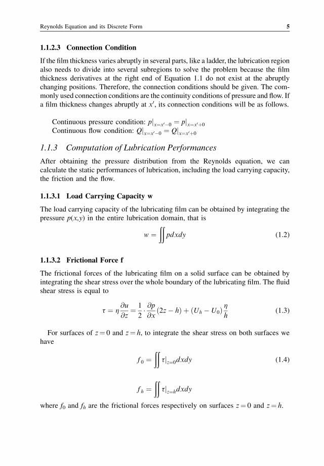
1.1.3 Computation of Lubrication Performances

After obtaining the pressure distribution from the Reynolds equation, we can

calculate the static performances of lubrication, including the load carrying capacity,

the friction and the flow.

1.1.3.1 Load Carrying Capacity w

The load carrying capacity of the lubricating film can be obtained by integrating the

pressure p(x,y) in the entire lubrication domain, that is

w ¼ðð

pdxdy (1.2)

1.1.3.2 Frictional Force f

The frictional forces of the lubricating film on a solid surface can be obtained by

integrating the shear stress over the whole boundary of the lubricating film. The fluid

shear stress is equal to

t ¼ h@u

@z¼ 1

2� @p@x

2z� hð Þ þ Uh � U0ð Þ hh

(1.3)

For surfaces of z¼ 0 and z¼ h, to integrate the shear stress on both surfaces we

have

f 0 ¼ðð

tjz¼0dxdy (1.4)

f h ¼ðð

tjz¼hdxdy

where f0 and fh are the frictional forces respectively on surfaces z¼ 0 and z¼ h.

Reynolds Equation and its Discrete Form 5

After the frictional forces have been obtained, we then can determine the friction

coefficientm¼ f/w as well as the frictional power loss and the heat due to the friction.

1.1.3.3 Lubricant Flow Q

The side leaking flows of lubricant can be obtained by integrating the flow rates

through the lubricating film boundary.

Qx ¼Ðqxdy

Qy ¼Ðqydx

(1.5)

By summing all leaking flows over all boundaries we can obtain the total flow,

which gives us the amount of lubricant needed to fill the clearance. At the same time,

the total leaking flow will influence the extent of convection so that we can calculate

the balanced thermal temperature according to leaking flow and friction power loss.

1.2 Reynolds Equations for Some Special Working Conditions

In Section 1.1, we have given the general form of the Reynolds equation. However, for

some specific engineering problems, the general Reynolds equation can be simplified,

which may make solving much easier. In the following, some forms of the Reynolds

equation for different conditions are given.

1.2.1 Slider and Thrust Bearing

Awedge slider is the simplest problem of lubrication design. If the geometry of the

slider is not very complicated, we can obtain an analytical solution. In addition,

through analysis of the slider problem, it will not only help us to understand the basic

characteristics of lubrication, but will also be useful for the thrust bearing lubrication

design.

Because the side leakage of lubricant need not be considered for solving an

infinitely wide slider, its Reynolds equation then can be simplified into a one-

dimensional ordinary differential equation:

d

dxh3

dp

dx

� �¼ 6Uh

dh

dx(1.6)

The common two-pressure boundary conditions of a slider are as follows.

pjx¼0 ¼ 0; pjx¼x0 ¼ 0 (x0 is the outlet boundary, x0 ¼ b; and b is the slider width).

pjx¼0 ¼ 0; pjx¼x0 ¼ 0 and@p

@x

��x¼x0

¼ 0 (x0 is the outlet boundary to be deter-

mined, x0 � b).


If the film thickness or its derivative is discontinuous, we should divide the

lubrication region into two parts at the discontinuous line so that the number of the

integral constants will correspondingly increase. Therefore, the connection conditions

must be used at the discontinuous line. If the discontinuous line is at x�, the connectionconditions will be:

Pressure continuous condition pjx¼x��0 ¼ pjx¼x�þ0 (1.7)

Flow continuous condition

� h3

12h

@p

@xþ ðU1 þ U2Þ h

2

� �x¼x��0

¼ � h3

12h

@p

@xþ ðU1 þ U2Þ h

2

� �x¼x�þ0

(1.8)

1.2.2 Journal Bearing

By spreading the journal bearing along the circumferential direction, we can

transform x into Ru so that the general form of the Reynolds equation is

@

R2@u

rh3

h� @p@u

� �þ @

@y

rh3

h� @p@y

� �¼ 6

@

R@uUrhð Þ þ @

@yVrhð Þ þ 2

@rh

@t

� �: (1.9)

The corresponding shape of the clearance can be expressed as:

h ¼ ecosu þ c ¼ cð1þ e cosuÞ (1.10)

where e is the eccentricity, c is the clearance of the radii of the bearing and the journal,

e¼ e/c is the eccentricity ratio and u is the circumferential coordinate starting from

the maximum film thickness position.

1.2.2.1 Infinitely Narrow Bearing

If the axial width of a bearing along the y direction is much less than the

circumferential length along the x direction, we have@p

@y� @p

R@uso that we can

set@p

R@u¼ 0. Because the film thickness h is only related to u, but independent of y, the

Reynolds equation becomes

d

dyh3 � dp

dy

� �¼ 6Uh

dh

Rdu(1.11)


The above Reynolds equation has only side boundary conditions. They are p¼ 0

at y ¼ � b

2and

dp

dy¼ 0 at y¼ 0 due to symmetry.

1.2.2.2 Infinitely Wide Bearing

We can approximately choosedp

dy¼ 0 for an infinitely wide bearing because the side

leakage can be ignored. Therefore, the Reynolds equation changes into an ordinary

differential equation.d

Rduh3

dp

Rdu

� �¼ 6Uh

dh

Rdu(1.12)

Its boundary conditions usually are pju¼0 ¼ 0, pju¼u2¼ 0 and

@p

@u

��u¼u2

¼ 0 (where

u2 is the outlet boundary to be determined, u2� 2p).

1.2.3 Hydrostatic Lubrication

The oil film for hydrostatic lubrication is formed by a fluid forced in under pressure

from the outside. Therefore, even if two lubricating surfaces have no relative motion,

a thick enough lubricating film can be achieved. The advantages of hydrostatic

lubrication are: (1) its load carrying capacity and the oil film thickness have no

relationship with the sliding velocity; (2) the film stiffness is so strong that it has a

very high accuracy; (3) its friction coefficient is so low that we can ignore the

influence of the static friction. The main disadvantages of hydrostatic lubrication are:

its structure is complex and a pressure oil supply systemmust be required which often

affects the working life and reliability of hydrostatic lubrication.

Substituting the condition of no relative sliding velocity into the Reynolds

Equation 1.1, we have the Reynolds equation for hydrostatic lubrication as follows

@

@x

rh3

h

@p

@x

� �þ @

@y

rh3

h

@p

@y

� �¼ 0 (1.13)

For a rectangular region, the outer pressure boundary conditions are usually

pjx¼0 ¼ 0; pjx¼l ¼ 0; pjy¼�b=2 ¼ 0; and the boundary pressure condition in the oil

chamber is: p¼ ps, where ps is the supplied oil pressure.

For a journal hydrostatic bearing, Reynolds Equation 1.13, the film thickness

equation and the boundary conditions can be solved easily in the form of cylindrical

coordinates. For solving the above equations, we can determine the variation

relationship between the load and the film thickness. Furthermore, if we consider

the working conditions, such as equal film thickness, incompressibility or isovis-

cosity, the Reynolds Equation 1.13 can be further simplified.


1.2.4 Squeeze Bearing

The relative sliding between two bearing surfaces is usually assumed to be zero when

analyzing squeeze lubrication, so that the Reynolds Equation 1.1 can be written as

follows

@

@xrh3

@p

@x

� �þ @

@yrh3

@p

@y

� �¼ 12h

@ðrhÞ@t

(1.14)

Usually, for a rectangular region, the boundary conditions are pjx¼0 ¼ 0; pjx¼l ¼ 0;

and pjy¼�b=2 ¼ 0. To solve the above equation we can determine the variation

relationship between the load and the film thickness.

1.2.5 Dynamic Bearing

Most actual bearings withstand a varying load whose direction, rotational speed or

other parameters change with time. Such bearings are collectively referred to as

dynamic bearing or nonstable load bearing. Obviously, the axis or the thrust plate of a

dynamic bearing moves along a certain trajectory. If the working parameters are

periodic functions of time, the trajectory of the axis is a complex and closed curve.

The working principles of the dynamic bearing can be divided into two types. The

first is where the journal does not rotate around its central axial, that is, there is no

relative sliding. Therefore, the journal axial moves along a certain trajectory under the

load. In this case, the journal and the bearing surfaces move mainly in the direction of

the film thickness so that the film pressure is generated by the squeeze effect. The

other type is where the journal rotates around its own center and the journal center

also moves. Therefore, the film pressure originates from the squeeze effect of these

two movements, that is, the journal rotation and the axis movement.

The general Reynolds equation for incompressible and dynamic lubrication is the

basic equation to analyze dynamic bearings. It can be written as follows

@

@x

h3

h

@p

@x

� �þ @

@y

h3

h

@p

@y

� �¼ 6U

@h

@xþ 12W (1.15)

In Equation 1.15 the first term on the right is the hydrodynamic effect; the second

term represents the squeeze effect; and when the Reynolds Equation 1.15 is applied

to a stable bearing, the term of the squeeze effect can be omitted, that is,

W ¼ wh � w0 ¼ @h

@t¼ 0:

The problemof calculating the axis trajectory of a dynamic bearing byEquation 1.15

belongs to an initial value problem. The stepping method is usually used to determine

the axis of the trajectory according to the given initial position of the axis.


1.2.6 Gas Bearing

The main feature of gas lubrication is that a gas is compressible. Therefore, the

density of the gas must be treated as a variable, that is, by using the Reynolds equation

for a variable density

@

@x

rh3

h

@p

@x

� �þ @

@y

rh3

h

@p

@y

� �¼ 6 U

@ðrhÞ@x

þ 2@ðrhÞ@t

� �(1.16)

Because the gas density varies with temperature and pressure, the ideal gas

equation can be expressed as follows

p

r¼ RT (1.17)

where T is the absolute temperature, and R is the gas constant which does not change

for a certain gas.

For a usual gas lubrication problem, gas lubrication can be regarded as an

isothermal process and this assumption has an error less than a few percent. For

such a problem, Equation 1.15 becomes

p ¼ kr (1.18)

where k is a proportional constant.

In addition, if a gas lubrication process is so fast that the heat cannot be conducted

in time, the process can be thought to be adiabatic. The gas state equation of the

adiabatic process is as follows

p ¼ krn (1.19)

where n is the gas specific heat ratio relate to the atomic number of the gas molecules.

For air, n¼ 1.4.

For an isothermal process, the Reynolds equation becomes

@

@xh3p

@p

@x

� �þ @

@yh3p

@p

@y

� �¼ 6h U

@

@xðphÞ þ 2

@

@tðphÞ

� �(1.20)

Equation 1.20 is the basic equation for solving gas lubrication problems.

1.3 Finite Difference Method of Reynolds Equation

If the boundary conditions are given for solving a differential equation, this is known

as a boundary value problem. In hydrodynamic lubrication calculations, the finite

difference method is commonly used to numerically solve the Reynolds equation. The

major steps of finite difference method are as follows.


1.3.1 Discretization of Equation

First, change the partial differential equations into dimensionless forms. This is

accomplished by expressing the variables in a universal form.

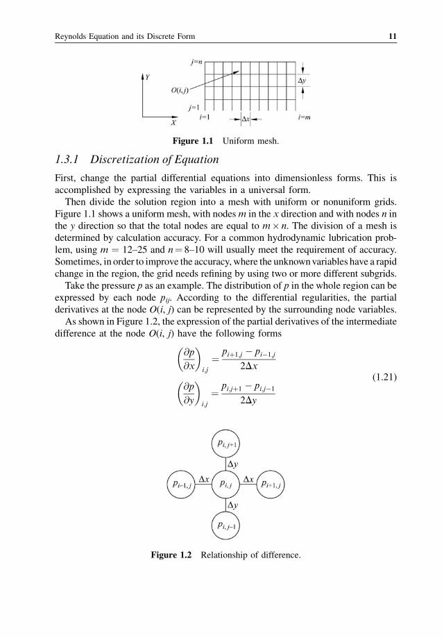
Then divide the solution region into a mesh with uniform or nonuniform grids.

Figure 1.1 shows a uniform mesh, with nodesm in the x direction and with nodes n in

the y direction so that the total nodes are equal to m� n. The division of a mesh is

determined by calculation accuracy. For a common hydrodynamic lubrication prob-

lem, using m ¼ 12–25 and n¼ 8–10 will usually meet the requirement of accuracy.

Sometimes, in order to improve the accuracy, where the unknownvariables have a rapid

change in the region, the grid needs refining by using two or more different subgrids.

Take the pressure p as an example. The distribution of p in the whole region can be

expressed by each node pij. According to the differential regularities, the partial

derivatives at the node O(i, j) can be represented by the surrounding node variables.

As shown in Figure 1.2, the expression of the partial derivatives of the intermediate

difference at the node O(i, j) have the following forms

@p

@x

� �i;j

¼ piþ1;j � pi�1;j

2Dx

@p

@y

� �i;j

¼ pi;jþ1 � pi;j�1

2Dy

(1.21)

Figure 1.1 Uniform mesh.

Figure 1.2 Relationship of difference.


The second-order partial derivatives of the intermediate difference are as follows

@2p

@x2

� �i;j

¼ piþ1;j þ pi�1;j � 2pi;j

ðDxÞ2

@2p

@y2

� �i;j

¼ pi;jþ1 þ pi;j�1 � 2pi;j

ðDyÞ2(1.22)

In order to obtain the unknown variables near the border, forward or backward

difference formulas are used as follows

@p

@x

� �i;j

¼ piþ1;j � pi;j

Dx

@p

@y

� �i;j

¼ pi;jþ1 � pi;j

Dy

(1.23)

@p

@x

� �i;j

¼ pi;j � pi�1;j

Dx

@p

@y

� �i;j

¼ pi;j � pi;j�1

Dy

(1.24)

Usually, the accuracy of the intermediate difference is high. The following

intermediate difference formulas can also be used in calculation

@p

@x

� �i;j

¼ piþ1=2;j � pi�1=2;j

Dx(1.25)

1.3.2 Difference Form of Reynolds Equation

According to the above formulas, the two-dimensional Reynolds equation can be

written in a standard form of the second-order partial differential equation

A@2p

@x2þ B

@2p

@y2þ C

@p

@xþ D

@p

@y¼ E (1.26)

where A, B, C, D and E are known parameters.

Equation 1.26 can be applied to each node. According to Equations 1.21 and 1.22,

the relationship of pressure pi,j at node O(i,j) with the adjacent pressures can be

written as follows

~pki;j ¼ CNpki;jþ1 þ CSp

kþ1i;j�1 þ CEp

kiþ1;j þ CWp

kþ1i�1;j þ G (1.27)

where, p with superscript k is the original pressure, and with superscript kþ1 is the

iterated one; and


numerical of lubrication

Documents