numerical modelling of heat and mass transfer and...
TRANSCRIPT

Numerical Modelling of
Heat and Mass Transfer
and Optimisation of a
Natural Draft Wet Cooling
Tower
By
N.J.Williamson
A Dissertation Submitted to
the School of Aerospace, Mechanical and Mechatronic
Engineering
The University of Sydney
in Fulfilment of the Requirements
for the Degree of
Doctor of Philosophy
Copyright c© N.J. Williamson 2008
All rights reserved

Declaration
I hereby declare that the work presented in this thesis is solely my own
work and that to the best of my knowledge, the work is original except
where otherwise indicated by reference to other authors or works. No part
of this work has been submitted for any other degree or diploma.
Nicholas Williamson
ii

Acknowledgements
There have been many people who have assisted, encouraged and supported
me during my PhD. In particular I wish to thank my supervisors Prof.
Steven Armfield and Prof. Masud Behnia for their guidance and advice
throughout this study. Prof. Behnia’s efforts in promoting collaboration
with other universities and research groups has led to many interesting op-
portunities during this study, to which I am very grateful. He has also been
very supportive in looking after my interests and the many other aspects of
PhD life. I could also not ask for better colleagues to work with than Steve
Armfield and Michael Kirkpatrick. Their enthusiasm for so many aspects of
fluid mechanics, their wide ranging knowledge and insightful comments and
suggestions have been both inspiring and motivating. I am glad to have had
the opportunity to work with them both.
I would also like to thank Dr. Kloppers and Prof. Kroger for their sup-
port with empirical correlations, their helpful suggestions and their kindness
in South Africa as hosts. Their general interest in this project is much ap-
preciated.
I wish to thank Peter Wormald and the plant performance group at
Delta Electricity for their support during the initial stages of this study,
particularly for supplying plant performance data and the manufacturers
information on the cooling towers which this study is based on.
In addition I would like to thank my other colleagues at the University of
Sydney fluid dynamics research group for their assistance in everything from
performing my first linux installation and finding helpful latex packages to
organising a good Christmas BBQ.
Finally I would like to thank my family and other friends for their encour-
agement, particularly Radhika for her patience, good humour and unfailing
interest in my work.
iii

Abstract
The main contribution of this work is to answer several important questions
relating to natural draft wet cooling tower (NDWCT) modelling, design and
optimisation.
Specifically, the work aims to conduct a detailed analysis of the heat
and mass transfer processes in a NDWCT, to determine how significant the
radial non-uniformity of heat and mass transfer across a NDWCT is, what
the underlying causes of the non-uniformity are and how these influence
tower performance. Secondly, the work aims to determine what are the con-
sequences of this non-uniformity for the traditional one dimensional design
methods, which neglect any two-dimensional air flow or heat transfer effects.
Finally, in the context of radial non-uniformity of heat and mass transfer,
this work aims to determine the optimal arrangement of fill depth and wa-
ter distribution across a NDWCT and to quantify the improvement in tower
performance using this non-uniform distribution.
To this end, an axisymmetric numerical model of a NDWCT has been
developed. A study was conducted testing the influence of key design and op-
erating parameters. The results show that in most cases the air flow is quite
uniform across the tower due to the significant flow restriction through the
fill and spray zone regions. There can be considerable radial non-uniformity
of heat transfer and water outlet temperature in spite of this. This is largely
due to the cooling load in the rain zone and the radial air flow there. High
radial non-uniformity of heat transfer can be expected when the cooling load
in the rain zone is high. Such a situation can arise with small droplet sizes,
low fill depths, high water flow rates. The results show that the effect of
tower inlet height on radial non-uniformity is surprisingly very small. Of
the parameters considered the water mass flow rate and droplet size and
droplet distribution in the rain zone have the most influence on radial non-
iv

v
uniformity of heat transfer.
The predictions of the axisymmetric numerical model have been com-
pared with a one dimensional NDWCT model. The difference between the
predictions of tower cooling range is very low, generally around 1-2%. This
extraordinarily close comparison supports the assumptions of one dimen-
sional flow and bulk averaged heat transfer implicit in these models. Under
the range of parameters tested here the difference between the CFD models
predictions and those of the one dimensional models remained fairly constant
suggesting that there is no particular area where the flow/heat transfer be-
comes so skewed or non-uniform that the one dimensional model predictions
begin to fail.
An extended one dimensional model, with semi-two dimensional capabil-
ity, has been developed for use with an evolutionary optimisation algorithm.
The two dimensional characteristics are represented through a radial profile
of the air enthalpy at the fill inlet which has been derived from the CFD
results. The resulting optimal shape redistributes the fill volume from the
tower centre to the outer regions near the tower inlet. The water flow rate
is also increased here as expected, to balance the cooling load across the
tower, making use of the cooler air near the inlet. The improvement has
been shown to be very small however. The work demonstrates that, con-
trary to common belief, the potential improvement from multi-dimensional
optimisation is actually quite small.

List of Publications
Journal Papers
1. Williamson, N., Armfield, S. and Behnia, M. Numerical simulation of
flow in a natural draft wet cooling tower - the effect of radial ther-
mofluid fields, Applied Thermal Engineering (2007) (IN PRESS).
2. Williamson, N., Behnia, M. and Armfield, S. Comparison of a 2D
axisymmetric CFD model of a natural draft wet cooling tower and
a 1D model, International Journal of Heat and Mass Transfer (2007)
(under review).
3. Williamson, N., Behnia, M. and Armfield, S. Optimal annular fill and
water flow rate profile in a natural draft wet cooling tower, Interna-
tional Journal of Energy Research (2007) (under review).
4. Williamson, N., Al-Waked, R., Behnia, M. and Armfield, S. Thermal
performance of natural draft cooling towers, Energy Conversion and
Management (2007) (submitted).
Conference Papers
1. Williamson, N., Al-Waked, R., Behnia, M. and Armfield, S. Simula-
tion of heat and mass transfer inside a natural wet draft cooling tow-
ers under cross-wind conditions, Proceedings of the 3rd International
Conference on Heat Transfer, Fluid Mechanics and Thermodynamics,
Cape Town, South Africa, 21-24 June 2004.
2. Williamson, N., Behnia, M. and Armfield, S. Numerical simulation
of heat and mass transfer in a natural draft wet cooling tower, Pro-
vi

vii
ceedings of the 15th Australasian Fluid Mechanics Conference, The
University of Sydney, Sydney, Australia, 13-17 December 2004.
3. Williamson, N., Behnia, M. and Armfield, S. Numerical simulation
of heat and mass transfer in a natural draft wet cooling tower, Pro-
ceedings of 4th International Conference on Computational Heat and
Mass Transfer, 4th International Conference on Computational Heat
and Mass Transfer, Paris-Cachan, France, 17-20 May 2005.
4. Williamson, N., Behnia, M. and Armfield, S. Numerical simulation
of heat and mass transfer in a natural draft wet cooling tower and
comparisons with existing one-dimensional methods, 4th International
Conference on Heat Transfer, Fluid Mechanics and Thermodynamics,
University of Pretoria, Pretoria, South Africa, 19-20 September 2005.
5. Williamson, N., Armfield, S. and Behnia, M. The importance of inlet
height to the performance of a natural draft wet cooling tower, 8th
Australasian Heat and Mass Transfer Conference, Curtin University
of Technology, Perth, Western Australia 26-29 July 2005.
6. Williamson, N., Al-Waked, R., Behnia, M. and Armfield, S. Thermal
performance of natural draft cooling towers, 18th International Sym-
posium on Transport Phenomena, Daejeon, Korea, 27-30 August, 2007
(Invited Keynote Paper).
Contents
Contents viii
List of Figures xii
List of Tables xv
Nomenclature xvi
1 Introduction 1
1.1 Background . . . . . . . . . . . . . . . . . . . . . . . . . . . . 1
1.2 Value of performance . . . . . . . . . . . . . . . . . . . . . . . 4
1.3 Previous work . . . . . . . . . . . . . . . . . . . . . . . . . . . 5
1.4 Extent of this study . . . . . . . . . . . . . . . . . . . . . . . 10
1.5 Thesis layout . . . . . . . . . . . . . . . . . . . . . . . . . . . 11
2 Heat and Mass Transfer Theory 13
2.1 Introduction . . . . . . . . . . . . . . . . . . . . . . . . . . . . 13
2.2 Flow description . . . . . . . . . . . . . . . . . . . . . . . . . 14
2.3 Simultaneous heat and mass transfer . . . . . . . . . . . . . . 15
2.4 Merkel model . . . . . . . . . . . . . . . . . . . . . . . . . . . 17
2.5 Discussion of model validity . . . . . . . . . . . . . . . . . . . 18
2.6 Poppe model . . . . . . . . . . . . . . . . . . . . . . . . . . . 20
2.7 Other models . . . . . . . . . . . . . . . . . . . . . . . . . . . 23
2.8 Discussion . . . . . . . . . . . . . . . . . . . . . . . . . . . . . 23
2.9 Empirical transfer coefficients . . . . . . . . . . . . . . . . . . 24
3 Computational Fluid Dynamics 26
3.1 Introduction . . . . . . . . . . . . . . . . . . . . . . . . . . . . 26
3.2 Computational fluid dynamics . . . . . . . . . . . . . . . . . . 26
viii

CONTENTS ix
3.3 Continuity and momentum equations . . . . . . . . . . . . . . 27
3.4 Turbulence modelling . . . . . . . . . . . . . . . . . . . . . . 27
3.5 RANS turbulence modelling . . . . . . . . . . . . . . . . . . . 29
3.5.1 k − ǫ transport equations . . . . . . . . . . . . . . . . 30
3.5.2 Heat and mass transfer modelling . . . . . . . . . . . . 31
3.6 Axisymmetric equations . . . . . . . . . . . . . . . . . . . . . 32
3.7 Numerical solution procedure . . . . . . . . . . . . . . . . . . 33
4 LES of Scalar Transport 36
4.1 Introduction . . . . . . . . . . . . . . . . . . . . . . . . . . . . 36
4.2 Background . . . . . . . . . . . . . . . . . . . . . . . . . . . . 37
4.3 Sub-filter-scale stress models . . . . . . . . . . . . . . . . . . 39
4.4 Sub-filter-scale heat flux modelling . . . . . . . . . . . . . . . 41
4.5 Governing equations . . . . . . . . . . . . . . . . . . . . . . . 42
4.5.1 Implicitly filtered SGS models . . . . . . . . . . . . . . 43
4.5.2 Explicit filtered SGS models (DMM and DRM) . . . . 45
4.6 Channel flow simulation . . . . . . . . . . . . . . . . . . . . . 47
4.7 Results and discussion . . . . . . . . . . . . . . . . . . . . . . 49
4.8 Conclusions . . . . . . . . . . . . . . . . . . . . . . . . . . . . 58
5 Two Dimensional NDWCT Model 60
5.1 Introduction . . . . . . . . . . . . . . . . . . . . . . . . . . . . 60
5.2 Model description . . . . . . . . . . . . . . . . . . . . . . . . . 60
5.3 Domain and boundary conditions . . . . . . . . . . . . . . . . 61
5.4 Solution procedure . . . . . . . . . . . . . . . . . . . . . . . . 63
5.5 Component losses . . . . . . . . . . . . . . . . . . . . . . . . . 64
5.6 Discrete phase model: rain and spray water flow modelling . 66
5.6.1 Droplet trajectory calculation . . . . . . . . . . . . . . 67
5.6.2 Heat and mass transfer . . . . . . . . . . . . . . . . . 68
5.6.3 Discrete phase-continuous phase coupling . . . . . . . 70
5.6.4 Spray and rain zone modelling . . . . . . . . . . . . . 71
5.7 Fill representation . . . . . . . . . . . . . . . . . . . . . . . . 73
5.7.1 Introduction . . . . . . . . . . . . . . . . . . . . . . . 73
5.7.2 Momentum sink . . . . . . . . . . . . . . . . . . . . . 74
5.7.3 Heat and mass transfer in the fill . . . . . . . . . . . . 77
5.7.4 Coupling procedure . . . . . . . . . . . . . . . . . . . 79
5.7.5 Model validation . . . . . . . . . . . . . . . . . . . . . 80
CONTENTS x
5.8 Domain and mesh independence studies . . . . . . . . . . . . 84
5.9 Model sensitivity . . . . . . . . . . . . . . . . . . . . . . . . . 86
5.10 Validation . . . . . . . . . . . . . . . . . . . . . . . . . . . . . 87
5.11 Results . . . . . . . . . . . . . . . . . . . . . . . . . . . . . . . 88
5.12 Conclusions . . . . . . . . . . . . . . . . . . . . . . . . . . . . 94
6 Sensitivity of Key Parameters 97
6.1 Introduction . . . . . . . . . . . . . . . . . . . . . . . . . . . . 97
6.2 Results . . . . . . . . . . . . . . . . . . . . . . . . . . . . . . . 97
6.2.1 Reference conditions . . . . . . . . . . . . . . . . . . . 98
6.2.2 Water flow rate . . . . . . . . . . . . . . . . . . . . . . 102
6.2.3 Fill depth . . . . . . . . . . . . . . . . . . . . . . . . . 103
6.2.4 Tower inlet height . . . . . . . . . . . . . . . . . . . . 103
6.2.5 Ambient air condition . . . . . . . . . . . . . . . . . . 113
6.2.6 Droplet diameter . . . . . . . . . . . . . . . . . . . . . 116
6.3 Conclusions . . . . . . . . . . . . . . . . . . . . . . . . . . . . 117
7 One Dimensional Model 123
7.1 Introduction . . . . . . . . . . . . . . . . . . . . . . . . . . . . 123
7.2 Previous work . . . . . . . . . . . . . . . . . . . . . . . . . . . 123
7.3 One dimensional model . . . . . . . . . . . . . . . . . . . . . 125
7.3.1 Fill transfer and loss coefficients . . . . . . . . . . . . 126
7.3.2 Rain zone coefficients . . . . . . . . . . . . . . . . . . 128
7.3.3 Spray zone coefficients . . . . . . . . . . . . . . . . . . 129
7.3.4 Additional system losses . . . . . . . . . . . . . . . . . 130
7.4 Model procedure . . . . . . . . . . . . . . . . . . . . . . . . . 131
7.5 Results and discussion . . . . . . . . . . . . . . . . . . . . . . 131
7.5.1 Inlet height . . . . . . . . . . . . . . . . . . . . . . . . 133
7.5.2 Fill depth . . . . . . . . . . . . . . . . . . . . . . . . . 134
7.5.3 Water flow rate . . . . . . . . . . . . . . . . . . . . . . 135
7.6 Rain zone correlation . . . . . . . . . . . . . . . . . . . . . . . 137
7.7 Sensitivity of performance to Merkel number . . . . . . . . . 140
7.8 Poppe model comparison . . . . . . . . . . . . . . . . . . . . 140
7.9 Conclusion . . . . . . . . . . . . . . . . . . . . . . . . . . . . 141

CONTENTS xi
8 Two Dimensional Optimisation 143
8.1 Introduction . . . . . . . . . . . . . . . . . . . . . . . . . . . . 143
8.2 Previous work . . . . . . . . . . . . . . . . . . . . . . . . . . . 144
8.3 Extended one-dimensional-zonal model . . . . . . . . . . . . . 146
8.4 Model procedure . . . . . . . . . . . . . . . . . . . . . . . . . 150
8.5 Problem description . . . . . . . . . . . . . . . . . . . . . . . 152
8.6 Evolutionary algorithm procedure . . . . . . . . . . . . . . . . 152
8.6.1 Selection operators . . . . . . . . . . . . . . . . . . . . 153
8.6.2 Mutation operators . . . . . . . . . . . . . . . . . . . . 153
8.6.3 Crossover operators . . . . . . . . . . . . . . . . . . . 154
8.7 Results and discussion . . . . . . . . . . . . . . . . . . . . . . 155
8.8 Conclusions . . . . . . . . . . . . . . . . . . . . . . . . . . . . 160
9 Conclusions 161
9.1 Study results and objectives . . . . . . . . . . . . . . . . . . . 161
9.2 Closing discussion and significant results . . . . . . . . . . . . 165
9.3 Recommendations for further work . . . . . . . . . . . . . . . 167
Bibliography 168
Appendices
A Merkel and Poppe Equation Derivation 180
B Thermophysical Fluid Properties 186
C Tower Draft Calculation 193

List of Figures
1.1 Power station cycle with cooling tower . . . . . . . . . . . . . 2
1.2 Natural draft wet cooling tower structure . . . . . . . . . . . 3
1.3 Natural draft wet cooling tower heat and mass transfer zones 3
2.1 Air flow over a vertical water film . . . . . . . . . . . . . . . . 15
2.2 Incremental control volume of the fill . . . . . . . . . . . . . . 16
2.3 Merkel solver procedure in fill test procedure (a) and subse-
quent tower performance evaluation (b) . . . . . . . . . . . . 19
2.4 Poppe solver procedure in fill test procedure (a) and subse-
quent tower performance evaluation (b) . . . . . . . . . . . . 22
3.1 Flow variables stored on collocated grid, with scalar and vec-
tor quantities stored at cell centres . . . . . . . . . . . . . . . 35
4.1 Periodic channel flow configuration . . . . . . . . . . . . . . . 43
4.2 Mean streamwise velocity profile, for mesh A (a) and for mesh
B (b) . . . . . . . . . . . . . . . . . . . . . . . . . . . . . . . 50
4.3 Mean temperature profile . . . . . . . . . . . . . . . . . . . . 52
4.4 Rxy Reynolds stress . . . . . . . . . . . . . . . . . . . . . . . 53
4.5 Traceless Reynolds stress on mesh A . . . . . . . . . . . . . . 55
4.6 Resolved and modelled temperature flux, hy = 〈v′φ′〉/uτTτ +
〈γy〉/uτTτ on mesh A (a) and (b) and mesh B (c) . . . . . . . 56
4.7 Model subgrid heat flux hy for mesh A . . . . . . . . . . . . . 57
5.1 Computational domain details . . . . . . . . . . . . . . . . . . 63
5.2 Segregated solver procedure . . . . . . . . . . . . . . . . . . . 65
5.3 Model representation of pressure loss terms . . . . . . . . . . 66
5.4 Coupling of droplet flow with continuous phase model . . . . 67
xii

LIST OF FIGURES xiii
5.5 Condensation routine procedure . . . . . . . . . . . . . . . . . 71
5.6 Spray droplet trajectories at centre of tower coloured by tem-
perature . . . . . . . . . . . . . . . . . . . . . . . . . . . . . . 72
5.7 Schematic of fill representation . . . . . . . . . . . . . . . . . 74
5.8 Validation of the fill model . . . . . . . . . . . . . . . . . . . 82
5.9 Validation of the fill model . . . . . . . . . . . . . . . . . . . 83
5.10 Mesh detail . . . . . . . . . . . . . . . . . . . . . . . . . . . . 85
5.11 Model validation . . . . . . . . . . . . . . . . . . . . . . . . . 87
5.12 Radial velocity profile . . . . . . . . . . . . . . . . . . . . . . 88
5.13 Vector plots of air flow in the tower . . . . . . . . . . . . . . . 89
5.14 Stream lines entering the tower . . . . . . . . . . . . . . . . . 90
5.15 Contours of air temperature, humidity, velocity and pressure
in the rain zone . . . . . . . . . . . . . . . . . . . . . . . . . . 92
5.16 Contours of air temperature, humidity, velocity magnitude
and pressure . . . . . . . . . . . . . . . . . . . . . . . . . . . . 93
5.17 Merkel number profiles . . . . . . . . . . . . . . . . . . . . . . 95
5.18 Loss coefficient profiles . . . . . . . . . . . . . . . . . . . . . . 96
6.1 Flow profiles with variable water flow rate . . . . . . . . . . . 99
6.2 Flow profiles with variable water flow rate . . . . . . . . . . . 100
6.3 Specific humidity profile with variable water flow rate . . . . 101
6.4 Flow profiles with variable fill depth . . . . . . . . . . . . . . 104
6.5 Flow profiles with variable fill depth . . . . . . . . . . . . . . 105
6.6 Flow profiles with variable fill depth . . . . . . . . . . . . . . 106
6.7 Radial velocity profile . . . . . . . . . . . . . . . . . . . . . . 107
6.8 Flow profiles with variable tower inlet height . . . . . . . . . 108
6.9 Flow profiles with variable tower inlet height . . . . . . . . . 109
6.10 Flow profiles with variable tower inlet height . . . . . . . . . 110
6.11 Droplet mass source in rain zone . . . . . . . . . . . . . . . . 111
6.12 Droplet sensible heat source in rain zone . . . . . . . . . . . . 112
6.13 Flow profiles with variable ambient air temperature and hu-
midity . . . . . . . . . . . . . . . . . . . . . . . . . . . . . . . 114
6.14 Flow profiles with variable ambient air temperature and hu-
midity . . . . . . . . . . . . . . . . . . . . . . . . . . . . . . . 115
6.15 Flow profiles with variable ambient air temperature and hu-
midity . . . . . . . . . . . . . . . . . . . . . . . . . . . . . . . 116

LIST OF FIGURES xiv
6.16 Flow profiles with variable droplet diameter . . . . . . . . . . 118
6.17 Flow profiles with variable droplet diameter . . . . . . . . . . 119
6.18 Flow profiles with variable droplet diameter . . . . . . . . . . 120
6.19 Contours of air temperature with droplet distribution . . . . 121
7.1 Schematic representation of tower with flow resistance repre-
sented as loss coefficients . . . . . . . . . . . . . . . . . . . . . 126
7.2 1D NDWCT model solver procedure . . . . . . . . . . . . . . 132
7.3 Incremental Merkel number plotted against inlet height . . . 134
7.4 Incremental cooling range plotted against inlet height . . . . 135
7.5 Incremental Merkel number plotted against fill depth . . . . . 136
7.6 Incremental cooling range plotted against fill depth . . . . . . 136
7.7 Incremental Merkel number plotted against water flow rate . 137
7.8 Incremental cooling range plotted against water flow rate . . 138
7.9 Merkel number interpreted from CFD results compared with
correlation in Kroger [1] . . . . . . . . . . . . . . . . . . . . . 139
7.10 Water outlet temperature with Merkel number . . . . . . . . 140
8.1 Schematic of air flow in 1D zonal model . . . . . . . . . . . . 146
8.2 Profile of air enthalpy across the tower at the fill air inlet . . 148
8.3 Profile of air enthalpy across the tower at the fill air inlet . . 149
8.4 1D-zonal model solver procedure . . . . . . . . . . . . . . . . 151
8.5 Schematic representation of the evolutionary algorithm pro-
cedure . . . . . . . . . . . . . . . . . . . . . . . . . . . . . . . 153
8.6 Flow profiles under optimal parameters . . . . . . . . . . . . 158
8.7 Flow profiles under optimal parameters . . . . . . . . . . . . 159
C.1 Schematic representation of tower . . . . . . . . . . . . . . . . 193
List of Tables
3.1 Model coefficients for k − ǫ turbulence model . . . . . . . . . 31
4.1 Computational domain . . . . . . . . . . . . . . . . . . . . . . 48
4.2 Bulk statistics . . . . . . . . . . . . . . . . . . . . . . . . . . . 51
5.1 Design parameters for the reference tower . . . . . . . . . . . 62
5.2 Relaxation parameters . . . . . . . . . . . . . . . . . . . . . . 64
5.3 Droplet distribution in the rain zone . . . . . . . . . . . . . . 73
5.4 Test parameters . . . . . . . . . . . . . . . . . . . . . . . . . 81
5.5 Comparison of water outlet temperature predictions from Poppe
method and a CFD test section . . . . . . . . . . . . . . . . . 84
5.6 Fill model column width . . . . . . . . . . . . . . . . . . . . . 84
5.7 Grid independence . . . . . . . . . . . . . . . . . . . . . . . . 84
5.8 Sensitivity of model to spray parameters . . . . . . . . . . . . 86
7.1 Range over which Eqn. 7.11 and 7.12 are valid . . . . . . . . 129
8.1 Evolutionary algorithm operator probabilities and parameters 154
8.2 Optimal design parameters . . . . . . . . . . . . . . . . . . . 156
B.1 Specific heat polynomial coefficients . . . . . . . . . . . . . . 190
B.2 Viscosity polynomial coefficients . . . . . . . . . . . . . . . . 191
B.3 Thermal conductivity polynomial coefficients . . . . . . . . . 192
xv

Nomenclature
Variables
A wetted contact area (m2)
a fill area density (−)
C molar concentration (kgmol/m3)
CD drag coefficient (−)
Cf skin friction coefficient (-)
Cp specific heat (kJ/kgK)
d diameter (m)
Dm diffusion coefficient of vapour in air (m2/s)
G mass flow rate per unit area (mass flux) (kg/s/m2)
g gravitational acceleration (m/s2)
H height (m)
h volumetric heat transfer coefficient (W/m2K)
hD mass transfer coefficient (m/s)
hm volumetric mass transfer coefficient (kg/m2s)
i enthalpy (kJ/kg)
i′′ enthalpy of saturated air (kJ/kg)
i′′′ enthalpy of super saturated air (kJ/kg)
xvi

NOMENCLATURE xvii
ifgwo latent heat of water evaluated at 0◦C (kJ/kg)
K loss coefficient (−)
k turbulent kinetic energy (m2/s2)
k∞ thermal conductivity of the continuous phase (W/mK)
Lfi depth of the fill (m)
Lef Lewis factor (= h/hmCpm)
M molecular weight (kg/kgmol)
m mass flow rate (kg/s)
mcond rate of condensation (kg/s)
mevap water evaporation rate (kg/s)
Me Merkel number (−)
MeP Merkel number from Poppe equations (−)
N molar flux (kgmol/m2s)
Nu Nusselt number (-)
P pressure (Pa)
Pr Prandtl number (=Cpµ/k∞)
Prt Turbulent Prandtl number (-)
R universal gas constant (N · m/kmol · K)
r radius (m)
Re Reynolds number (= ρD(U)/µ)
S source term
Sc Schmidt number (= µ/ρDm)
Sct Turbulent Schmidt number (-)
Sh Sherwood number (= hDdd/Dm)

NOMENCLATURE xviii
T temperature (K)
Trange tower range temperature (= Tw,i − Tw,o) (K)
u velocity vector (m/s)
V velocity of the air flow in the fill (m/s)
X mass fraction (−)
Greek Letters
αk kinetic energy coefficient(−)
δ residual error
ǫ turbulent kinetic energy dissipation rate (m2/s3)
Γ diffusion coefficient (kg/ms)
µ viscosity (kg/ms)
ω specific humidity (kg water vapour/kg dry air)
ω′′ specific humidity of saturated air (kg water vapour/kg dry air)
φ flow variable
ρ density (kg/m3)
σ surface tension (N/m)
Subscripts
a air
ct cooling tower loss
ctc cooling tower contraction before fill
cte cooling tower expansion after fill
cts tower supports
d droplet
de drift eliminators

NOMENCLATURE xix
fi fill
fs fill supports
∞ ambient surroundings
i inlet
ma air-water vapour mixture
mom momentum
o outlet
p Poppe format
q energy
rz rain zone
s at the surface
sat at saturation
sp spray zone
Ta at air temperature
to tower outlet
Tw at water temperature
v vapour
w water
wdn water distribution network
Acronyms
CFD computational fluid dynamics
DNS direct numerical simulation
DPM discrete phase model
LES large eddy simulation

NOMENCLATURE xx
NDWCT natural draft wet cooling tower
RANS Reynolds averaged Navier Stokes equations
SFS sub-filter-scale
SGS sub-grid-scale

Chapter 1
Introduction
1.1 Background
Cooling towers are an integral part of many industrial processes. Their
purpose is to reject waste heat. They are often used in power generation
plants to cool the condenser feed-water as shown in Fig. 1.1. Here, the
cooling tower uses ambient air to cool warm water from the condenser in a
secondary cycle.
There are many cooling tower designs or configurations. In dry cooling
towers the water is passed through finned tubes forming a heat exchanger so
only sensible heat is transfered to the air. In wet cooling towers the water
is sprayed directly into the air so evaporation occurs and both latent heat
and sensible heat are exchanged. In a hybrid tower a combination of both
approaches are used. Cooling towers can further be categorised into forced
or natural draft towers. Forced units tend to be relatively small structures
where the air flow is driven by fan.
In a natural draft cooling tower the air flow is generated by natural
convection only. The draft is established by the density difference between
the warm air inside the tower and the cool dense ambient air outside the
tower. In a wet cooling tower, the water vapour inside the tower contributes
to the buoyancy and tower draft.
A further classification is between counter-flow and cross-flow cooling
towers. In cross-flow configuration, the air flows at some angle to water flow
whereas in counter-flow the air flows in the opposite direction to water flow.
More details on these systems can be found in [1]. This study is concerned
1

CHAPTER 1. INTRODUCTION 2
Natural DraftCooling Tower
Boiler
Turbine Generator
CondenserBoilerfeedwater
pump
Condenserfeedwaterpump
Figure 1.1: Power station cycle with cooling tower
with natural draft wet cooling towers (NDWCT) in counter-flow configura-
tion such as shown in Fig. 1.2. These structures are most commonly found
in power generation plants.
In a NDWCT in counter flow configuration, there are three heat and
mass transfer zones, the spray zone, the fill zone and the rain zone as shown
in Fig. 1.3. The water is introduced into the tower through spray nozzles
approximately 10m above the basin. The primary function of the spray zone
is simply to distribute the water evenly across the tower. The water passes
through a small spray zone as small fast moving droplets before entering the
fill.
There are a range of fill types. Generally they tend to be either a splash
bar fill type or film fill type. The splash bar type acts to break up water
flow into smaller droplets with splash bars or other means. A film fill is
a more modern design which forces the water to flow in film over closely
packed parallel plates [1, 2]. This significantly increases the surface area for
heat and mass transfer.
As the water leaves the fill and enters the rain zone, the water film breaks
up into droplets again before it is finally collected in the basin below the

CHAPTER 1. INTRODUCTION 3
1
2
3
4
6 6
�-
����
Tower Outlet
Shell
Wall
Figure 1.2: Natural draft wet cooling tower structure with cutaway section:(1) drift eliminators, (2) spray nozzles, (3) fill , (4) basin
Rain Zone
Fill Zone
Spray Zone
Air Flow
�
�
Figure 1.3: Natural draft wet cooling tower heat and mass transfer zones
CHAPTER 1. INTRODUCTION 4
tower.
The air enters the tower radially through the rain zone where it initially
flows in a part counter flow part cross flow manner before being drawn
axially into the fill and up into the tower. The air leaving the fill is generally
supersaturated [1, 3]. Drift eliminators are placed above the spray nozzles
to recover entrained water spray droplets in the flow.
A typical NDWCT has a tower height of around 130m, a base diameter
of 90m, with a flow rate of about 15000kg/s. About 2% of the water flow-
rate is evaporated; when attached to a thermal generation plant, about
1.6-2.5 litres of water is evaporated per kWh(e) generated [1]. A 600MW(e)
generation unit may require 25ML of makeup water in 24hrs to replace the
water evaporated in the cooling towers.
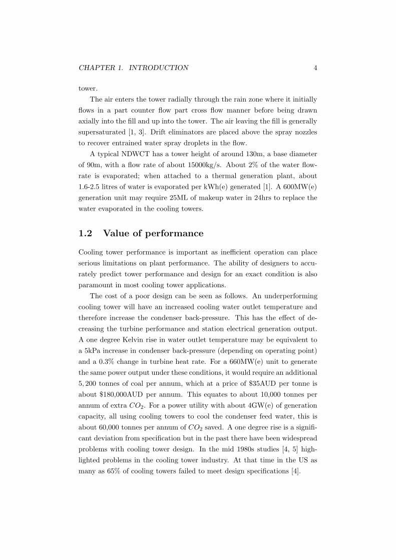
1.2 Value of performance
Cooling tower performance is important as inefficient operation can place
serious limitations on plant performance. The ability of designers to accu-
rately predict tower performance and design for an exact condition is also
paramount in most cooling tower applications.
The cost of a poor design can be seen as follows. An underperforming
cooling tower will have an increased cooling water outlet temperature and
therefore increase the condenser back-pressure. This has the effect of de-
creasing the turbine performance and station electrical generation output.
A one degree Kelvin rise in water outlet temperature may be equivalent to
a 5kPa increase in condenser back-pressure (depending on operating point)
and a 0.3% change in turbine heat rate. For a 660MW(e) unit to generate
the same power output under these conditions, it would require an additional
5, 200 tonnes of coal per annum, which at a price of $35AUD per tonne is
about $180,000AUD per annum. This equates to about 10,000 tonnes per
annum of extra CO2. For a power utility with about 4GW(e) of generation
capacity, all using cooling towers to cool the condenser feed water, this is
about 60,000 tonnes per annum of CO2 saved. A one degree rise is a signifi-
cant deviation from specification but in the past there have been widespread
problems with cooling tower design. In the mid 1980s studies [4, 5] high-
lighted problems in the cooling tower industry. At that time in the US as
many as 65% of cooling towers failed to meet design specifications [4].

CHAPTER 1. INTRODUCTION 5
This provides strong motivation to improve the heat and mass transfer
characteristics of power station cooling towers and produce reliable methods
to optimise and design them to specification.
1.3 Previous work
There have been few full scale experimental studies published due to the
expense and difficulty of working in operating cooling towers. Most cooling
tower manufacturers and operators treat the information as proprietary and
confidential. Sirok et al. [6] used a sophisticated measurement system to
map air flow rate and temperature profiles above the fill to plot efficiency
contours. The authors found local fouling blockages in the fill significantly
degraded performance in areas.
Scale models of NDWCT have been used for wind tunnel tests [7, 8] to
study the effect of cross wind on dry cooling tower performance, but in a
wet cooling tower it is impossible to achieve similarity with two phase flow
and heat and mass transfer.
The early study by Lowe and Christie [7] produced some of the first data
that quantified the non-uniformity of air flow across the fill. The authors
used scale isothermal test models to determine the velocity profile across
the tower and determined loss coefficients for a number of fill layouts in the
tower. The authors reduced the thickness of the model packing towards the
centre of the tower but found that it had little effect on the overall resistance
of the system. The results were validated with full scale data and found to
be reasonably comparable. The authors also expressed their opinion that in
very large towers the central area of the packing is ineffective because the
air has ”already been heated nearly to capacity” through the rain zone.
A significant number of studies have specifically addressed the combined
heat and mass transfer processes in a wet cooling tower and developed useful
non-dimensional transfer coefficients to rate tower performance [9–11]. The
validity and accuracy of these models has been the subject of much research.
The most famous of these is the Merkel [9] model, which contains simplifying
assumptions which introduce widely known inaccuracies [1, 12, 13]. Another
more accurate model was proposed by Poppe [10] which, although it avoided
the Merkel assumptions, has not been widely adopted. These are discussed
further in Chapter 2.

CHAPTER 1. INTRODUCTION 6
Tower modelling has traditionally been very simple, involving application
of one of the above thermal models with a simple hydraulic flow calculation
and treating the rest of the tower sometimes very superficially. Recently
published work has offered some improvement on these methods [14–17].
Kroger [1] and co-workers [3, 18–20] have produced the most advanced and
detailed one dimensional model in literature to date supported by a wealth
of experimental work on tower loss coefficients.
More recently numerical models have been developed. In most cases
these were multi-dimensional models which calculated the air flow field.
The very complex two-phase flow and heat transfer meant that NDWCT
modelling initially made use of many simplifying assumptions. Very early
work ignored the droplet flow in the rain zone and spray zone. Only recently
has it been made clear that the rain zone can provide up to 30% of the overall
cooling and the spray zone 5-10% [1].
No numerical models reported on to date explicitly model the fill, instead
researchers have employed source terms to model the effect of the fill on
the continuous phase [5, 21–25]. Usually empirical transfer coefficients are
used based on traditional heat and mass transfer methods as discussed in
Chapter 2. Frequently the Merkel model is used, primarily because acquiring
data in any other format is very difficult. The Merkel model has been so
widely adopted by industry and integrated into all the industry standards
that changing to a slightly better model is difficult, especially when under
most conditions, the Merkel model is sufficient [1, 3]. This has influenced
the development of many numerical models to date. Many of these models
(e.g. [22, 24]) use the Merkel model to derive separate energy and mass source
terms for scalar transport and continuity equations, even though this does
not make much sense. The Merkel model cannot be used to derive separate
mass and heat transfer coefficients or accurately specify a mass source term
because of the simplifications in its derivation. Other complete models such
as the Poppe model can be implemented easily and more accurately, as
they are a simple re-arrangement of the traditional heat and mass transfer
equations found in any standard text such as Mills [26].
The first two dimensional numerical CFD models of cooling towers began
to appear in literature in the 1980’s. Majumdar [24, 25] presented a two
dimensional finite difference model of flow in a natural draft and mechanical
draft wet cooling tower named VERA2D. The model employed an algebraic

CHAPTER 1. INTRODUCTION 7
turbulence model and used a heat and mass transfer calculation based on
the Merkel model. The model neglects water flow and heat transfer in the
rain and spray zones and does not take condensation into account. The
computational domain did not extend beyond the tower inlet or outlet so
the rain zone inlet air velocity profile would not have been accurate. As the
plume was not simulated the outlet pressure above the tower would also be
inaccurate.
Benton and Waldrop [27] developed a semi-two dimensional model em-
ploying the Bernoulli equation for calculating the air flow. The method was
less sophisticated than VER2D but could be run very economically using
the modest computer resources of the time.
Radosavljevic [5] presented both an axisymmetric and three dimensional
CFD model of a NDWCT employing an algebraic turbulence model and
found reasonable agreement with experimental data. Numerically, the model
was an advance on VERA2D [5]. The author reviewed the heat and mass
transfer models and included the effect of condensation on heat and mass
transfer. The heat and mass transfer in the spray and rain regions was
computed in the same manner as in the fill, with transfer characteristics
specified to calculate the overall source terms. The loss coefficients for these
zones were implemented in a similar manner. The author used a three
dimensional model to look at wind effects.
Other industry sponsored models have been produced as technical re-
ports and are cited by other authors [5, 24, 28]. In general, these are no
more advanced than VERA2D or Radosavljevic’s [5] work.
Fournier and Boyer [23] reported on a three dimensional numerical code
capable of modelling the two phase heat and mass transfer in cooling tow-
ers. The fill region was represented using source terms as functions of the
Poppe or Merkel equations. The water flow was not solved but its properties
were represented at discrete points on a one dimensional vertical grid. Ex-
change regions were setup where these water columns intersected the three
dimensional grid. At these points, the continuous phase (air/water mix-
ture) properties were mapped onto the one dimensional grid and the Poppe
or Merkel equations were solved to determine the change in water proper-
ties. Source terms were then interpolated back onto the three dimensional
grid to simulate the effect of the water on the air. The heat and mass trans-
fer in the rain region were modelled in a similar fashion, with the water
CHAPTER 1. INTRODUCTION 8
droplets assumed to travel in the vertical direction only and their effect on
the air flow expressed entirely through the axial momentum equation, with
no radial component included.
Hawlader and Liu [22] developed a two dimensional axisymmetric ND-
WCT model where the heat and mass transfer in the fill was represented
with the source terms as functions of the Merkel model. The spray zone
was neglected. The droplet flow in the rain zone was modelled using one-
dimensional Lagrangian particle tracking with source terms coupling the
heat, mass and momentum with the gas phase. The authors employed an
algebraic turbulence model. In this study the computational domain did not
extend beyond the tower inlet or tower outlet, again resulting in probable
errors in prediction of tower outlet pressure and rain zone inlet air velocity
profile.
More recently there has been significant interest in using numerical mod-
els to predict the effect of wind on both wet and dry natural draft cooling
towers and the effects of performance improving structures such as wind
break walls [18, 21, 29–39]. Most of the studies have examined dry cooling
towers. Al-Waked and Behnia present one of the few NDWCT studies, using
FLUENT [40]. The authors [21, 36–38] developed both a three dimensional
model of a NDDCT (natural draft dry cooling tower) and a NDWCT to
examine the effect of wind and performance improving structures such as
wind breaks and surrounding buildings. In the NDWCT model the authors
used a Lagrangian scheme, to model both the water flow in the fill and the
droplet phase, using the commercial CFD package FLUENT [40].
Other numerical models have simulated the buoyant plume from ND-
WCTs and spray drift with concern for the environmental impacts of the
plume and the spread of Legionaries disease [41, 42]. Other cooling tower
configurations such as small mechanical draft units and closed loop cooling
towers in heating ventilating and air-conditioning (HVAC) applications have
also received attention [43–47]. These studies have contributed very little to
the simulation of NDWCTs.
The accuracy to which the flow field is computed has improved as tur-
bulence models have advanced and computational power has increased. Un-
fortunately the availability of the data to validate the models has not pro-
gressed. No models to date achieve more detailed validation than a simple
comparison of the tower water outlet temperature with manufacturer’s data

CHAPTER 1. INTRODUCTION 9
or full scale measurements.
Kroger [1] postulates that a detailed one dimensional model is no worse
than the more complex two and three dimensional codes. Both one and
two/three dimensional models have a number of things in common. All
use empirical loss coefficients to represent tower features not able to be
physically represented in the model. These include drift eliminators, spray
nozzles, tower and fill supports and the fill itself. In addition, all models
use empirical transfer coefficient correlations to represent the water flow
in the fill as a source term on the gas phase. Some neglect the rain and
spray zones entirely and some model these regions in the same manner as
the fill [5, 22, 24, 25]. Few employ a limited Lagrangian particle tracking
restricting droplet flow to the vertical direction [22, 23]. In summary, even
the most complete two and three dimensional models are very empirical.
Their great advantage is that they can predict non uniform fill and water
flow distributions easily and they can provide more detail of thermal flow
phenomena in the tower. This comes at a significant computational price
however with run times orders of magnitude longer than for the one dimen-
sional models.
Currently, one dimensional models are usually employed to design cool-
ing towers [48–50]. There are a number of deficiencies with their use how-
ever, that have not been addressed. Across a NDWCT there is some radial
profile to the air flow and heat transfer as discussed in [1, 6, 7, 51] and as
clearly shown here in Chapter 6. Yet the effect of one dimensional flow as-
sumptions and the lumped heat transfer approach on the accuracy of a one
dimensional model of a NDWCT have not been examined to date. There
has been no detailed study examining the deficiencies of a one dimensional
model as compared to a model which calculates the multi-dimensional flow
field and heat transfer.
In addition, despite the number of numerical NDWCT models in liter-
ature, few examine the detail of the heat and mass transfer in the tower
and provide designers with immediate conclusions and recommendations to
produce better cooling towers. There has been no optimisation study in lit-
erature that considers two dimensional effects and the possibility of radially
varying the fill depth and water distribution.

CHAPTER 1. INTRODUCTION 10
1.4 Extent of this study
This study aims to answer the limitations outlined above. More specifically
the aims can be stated as:
1. Develop an advanced detailed CFD model of a NDWCT and further
the understanding of heat and mass transfer processes in the tower
and how they are coupled with the air flow field. Provide designers
with immediate conclusions on how tower performance is related to
key design parameters.
2. Examine a detailed one dimensional model and compare performance
predictions with a multi dimensional CFD model computing the air
flow field under a range of design parameters.
3. Quantify the improvement possible with multi-dimensional optimisa-
tion, by optimising the fill depth and water distribution radially across
the tower.
In this investigation, a more detailed model of a NDWCT has been de-
veloped that has the ability to resolve heat and mass transfer and air flow
locally in all regions of the tower. Such a model allows better understanding
of the integration of various system components in the tower and the cou-
pling of the heat and mass transfer. This model is an advance on previous
models, with the generality of the empirical correlations used and the detail
to which condensation is represented improved over previous efforts. The
water flow in the rain and spray zones has been modelled in more detail with
two-dimensional Lagrangian particle motion and the droplet distribution in
the rain zone represented.
The heat and mass transfer profiles are examined under a range of de-
sign conditions/parameters. In particular, the radial non-uniformity of heat
transfer due to local geometric effects and overall gradients in air tempera-
ture and flow rate are examined.
The overall model predictions are compared with those of a one dimen-
sional NDWCT model under the same range of conditions in an attempt
to understand the range of applicability of the one dimensional models and
where the models’ predictions diverge, if at all.
Finally, novel extentions to a one dimensional model are proposed al-
lowing semi-two dimensional behaviour to be captured without the time

CHAPTER 1. INTRODUCTION 11
penalties of the more complex CFD model. This model has been developed
and found to perform well compared to the CFD results under non-uniform
fill and water distribution. This model has been coupled with an evolu-
tionary optimisation procedure to determine the improvement possible by
optimising the fill depth and water distribution in two dimensions.
1.5 Thesis layout
Chapter One
Introduction to the thesis and overview natural draft wet cooling tower
design. The motivation for cooling tower research is discussed and previous
work summarised.
Chapter Two
A description of one dimensional heat and mass transfer and cooling tower
theory. The Merkel and Poppe methods are derived and aspects of the
methods discussed. The empirical forms of the fill transfer coefficients are
discussed.
Chapter Three
An introduction to computational fluid dynamics (CFD) and the numerics
of the commercial CFD package FLUENT [40] which has been employed in
this study. Turbulence modelling has been discussed in some detail.
Chapter Four
A background investigation on large eddy simulation (LES) turbulence mod-
elling is presented. This work is not directly related to the primary objectives
of this study but also forms a contribution to literature in the modelling of
scalar transport with LES.
Chapter Five
Description of the axisymmetric CFD model of a NDWCT developed in
this study. The fill model is compared with the one dimensional Poppe
method [10]. The importance of including the effects of condensation is
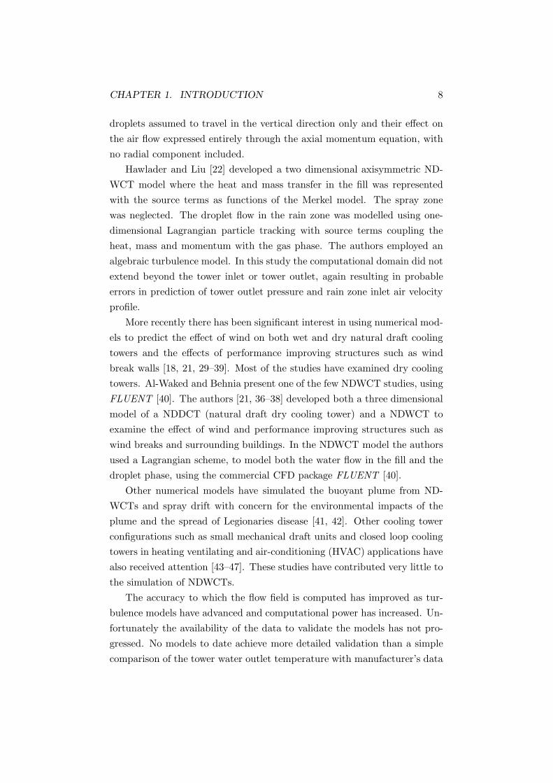
CHAPTER 1. INTRODUCTION 12
demonstrated. The validation of the model is discussed and results pre-
sented.
Chapter Six
The influence of key design and operating parameters on the performance
of the NDWCT and the radial non-uniformity of heat transfer across the
tower is investigated.
Chapter Seven
The CFD model is compared with a one dimensional NDWCT model with
the Merkel model employed for heat and mass transfer calculations. The
predictions of both models are compared under a range of design parameters.
Chapter Eight
A novel one dimensional-zonal model is presented which retains partial two
dimensional resolution. This is used in conjunction with an evolutionary
optimisation routine to optimise the fill depth and water flow rate across
the tower.
Chapter Nine
The conclusions of the individual chapters are summarised with overall rec-
ommendations and conclusions discussed.

Chapter 2
Heat and Mass Transfer
Theory
2.1 Introduction
In this chapter, the traditional methods of modelling heat and mass transfer
in a cooling tower are introduced.
Wet cooling tower performance modelling and design has changed little
in the last 50 years. Traditional practises employ a one dimensional heat
and mass transfer model such as the Merkel model [1, 9, 50]. The original
Merkel model [1] simplifies the one dimensional heat and mass transfer equa-
tions down to an enthalpy difference by neglecting the reduction in water
mass flow rate caused by evaporation and taking the Lewis factor [52] to
be unity. This allows the differential equations to be numerically integrated
through the tower with a simple hand calculation. This approach has been
thoroughly reviewed, with its shortfalls well documented [1, 11–14, 53–57].
Poppe and Rogener [10] later proposed a complete and more accurate
set of equations accounting for the evaporation of water but requiring the
simultaneous numerical integration of three differential equations through
the heat transfer region. Numerous other methods have been proposed [11,
14, 54, 58], most of which are slight variations on these original methods.
While more advanced models have been presented and the limitations
of the original Merkel model are well known, its simplicity and industries’
considerable experience with it have helped maintain its popularity. This
method now forms the cornerstone of the cooling tower industry. Merkel’s
13

CHAPTER 2. HEAT AND MASS TRANSFER THEORY 14
approach is still the standard approach recommended in many reference
texts [1, 26, 50] and industry standards [48, 49]. Most fill transfer coefficient
correlations are obtained using this method.
In this study both the Poppe and Merkel models are used. The first half
of this chapter briefly presents a derivation and discussion of these methods.
The second half contains a discussion of the empirical form and functional
dependence of the transfer coefficient.
2.2 Flow description
Cooling tower theory relies on the simplification of a complex air/water flow
interaction to a simple one dimensional volumetric heat and mass balance
to which empirical correlations can be applied.
In a counter flow wet cooling tower, water falls vertically down through
the fill in a liquid film or as droplets falling through air. Air, driven by
tower draft or fan, rises vertically in the opposite direction. Heat and mass
is exchanged between the two phases at the interface as shown in Fig. 2.1.
Both evaporation and sensible heat transfer cool the water causing the air
temperature and humidity to increase with height through the fill or heat
transfer zones.
Closely examining the fluid properties at each horizontal slice in a film
type fill may reveal temperature and species concentration gradients in the
water film flow and in the air stream as shown in Fig. 2.1. This may be
more realistic in a film with laminar flow than for a highly mixed turbulent
film in a modern fill design however, the models developed here are limited
to one dimension and the following simplifications are made.
1. The temperature gradient within the liquid film is ignored and the
temperature is taken as the bulk average value (Tw) at each vertical
location.
2. Similarly, the air temperature and the species concentration of water
vapour within the air are assumed to be at their bulk average values
so that horizontal temperature and species concentration gradients are
ignored.
3. At the interface of the two phases there is assumed to be a thin vapour
film of saturated air at the water temperature [1, 26].

CHAPTER 2. HEAT AND MASS TRANSFER THEORY 15
Droplet
Water Film
Air Flow
Bulk Air Ta, ωa
Air Flow
Bulk Air Ta, ωa
VelocityProfile
TemperatureProfile
Tw
Fill Wall SpecificHumidityProfile
���
ω′′
Tw
ω
@@
@RSaturatedAir-VapourFilm, ω′′
Tw
��Bulk Water
Tw
Figure 2.1: Air flow over a vertical water film (left) and flow around a waterdroplet (right)
The above assumptions apply equally to the calculation for heat and
mass transfer from a droplet in the rain and spray zones.
2.3 Simultaneous heat and mass transfer
The derivation of both the Poppe and Merkel models begins with a simple
energy and mass balance for an incremental control volume in the fill as
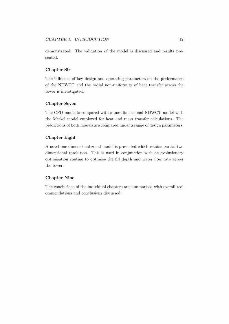
shown in Fig. 2.2. The change in contact area dA is found for the increment
dz using dA = afiAfrdz, where afi is the fill area density (wetted area
divided by volume of fill) and Afr is the frontal area of the fill. The change
in water mass flow rate dmw with respect to change in contact area is given
by,
dmw = hm(ω′′
(Tw) − ω) · dA, (2.1)
where ω is the specific humidity of air and hm is the mass transfer coefficient
(kg/m2s) and ω′′
(Tw) is the saturated specific humidity (kg/kg) at Tw (K).
A mass balance of an incremental step through the fill is given by,
madω + dmw = 0, (2.2)
where mw is the mass flow rate of water (kg/s) and ma is the dry air mass
flow rate in (kg/s).
CHAPTER 2. HEAT AND MASS TRANSFER THEORY 16
dz
water
mw + dmw
Tw + dTw
Tw, mw
air/vapour mixture
ima + dima
ma + (ω + dω)ma
dmw
h(Tw − Ta)dA
+iv,Twdmw
ima, ma + (ω)ma
dz
Tw,i, mw,i ima,o, ma + (ωo)ma
Tw, mw ima, ma + (ω)ma
Tw,o, mw,o ima,i, ma + (ωi)ma
Figure 2.2: Incremental control volume of the fill (left) and entire fill bound-ary conditions (right)
An energy balance taken from the water side yields,
madima − mwdiw − iwdmw = 0, (2.3)
where iw is the enthalpy of water and is given by CpwTw and ima is the
enthalpy of air/water vapour mixture (kJ/kg).
The energy balance viewed from the air stream is given by,
madima = ivdmw + h(Tw − Ta)dA, (2.4)
where h is the heat transfer coefficient (W/m2K). iv is the enthalpy of water
vapour (J/kg) at the water temperature and is given by,
iv = (ifgwo + CpvTw), (2.5)
where ifgwo is the enthalpy of vaporisation evaluated at zero degrees Cel-
sius (kJ/kg) and Cpv is the specific heat of water vapour (kJ/kgK). The
enthalpy of the system is therefore referenced to that of saturated water at
0◦C. ivdmw represents the enthalpy transfer resulting from mass transfer
and h(Tw − Ta)dA respresents sensible heat transfer.

CHAPTER 2. HEAT AND MASS TRANSFER THEORY 17
2.4 Merkel model
By making the following simplifying assumptions, the separate heat and
mass transfer phenomenon can be coupled into a single equation based on the
difference in enthalpy between the free air stream and the surface air/vapour
film:
1. Specific heats are constant.
2. The water evaporated from the water film does not effect the water
flow rate and is neglected from the water side energy balance.
3. The Lewis factor [52] for humid air is unity and constant.
A full derivation of what is usually referred to as Merkel’s equation is
given in Appendix A. The result can be written as,
Me =hmA
mw=
∫ Twi
Two
CpwdTw
(i′′ma(Tw ) − ima), (2.6)
where Me is the Merkel number, a non-dimensional performance coefficient
analogous to the NTU (Number of Transfer Units) of a heat exchanger [26].
It is also referred to as a transfer coefficient since it contains the mass transfer
coefficient together with the interface contact area.
The Merkel equation can be easily solved using a Chebyshev integration
technique as recommended in [1, 48] and using a simplified energy balance
(see Appendix A),dima
dTw=
mw
maCpw. (2.7)
The two equations are integrated together between the outlet and inlet water
temperatures, with i′′ma(Tw) (see Eqn. A.10) evaluated at every step. The
solver procedure for a fill test and subsequent tower performance evaluation
calculation is given in Fig. 2.3. In a fill performance test, the water inlet
and outlet temperatures (Tw,i and Tw,o), the water mass flow rate (mw), the
inlet air specific humidity (ωi) and temperature (Ta,i) and the dry air mass
flow rate (ma) are known. The Merkel number for the fill can be found by
straight forward integration of Eqn. 2.7 and Eqn. 2.6. In the subsequent
tower performance calculation, the Merkel number is known but the water
outlet temperature is not. In this case, the water outlet temperature must be

CHAPTER 2. HEAT AND MASS TRANSFER THEORY 18
guessed and checked through repetitive iteration until the calculated Merkel
number matches the specified Merkel number within a tolerance δMe .
The exact proportion of latent and sensible heat transfer is unknown
at any point in the fill, only the overall enthalpy transfer is known. This
means that the air enthalpy is calculated at each point but its humidity and
temperature are unknown. Usually the air is assumed to be saturated at the
exit and this allows the exit air temperature to be approximated. According
to Kloppers and Kroger [3] this is nearly always the case except under very
warm dry ambient conditions.
2.5 Discussion of model validity
As the commonly used model, Merkel theory has been extensively reviewed
[3, 13, 26, 53, 54, 59] since its conception in 1925 by Merkel. The method
has become the base for cooling tower design and specification because of its
simplicity, the accessibility of coefficients in this format and the method’s
useful non-dimensional form.
Sutherland [60] developed two numerical models to determine the effect
that ignoring water evaporation has on the accuracy of the Merkel model.
The author found that the tower volume was underestimated by between
5 and 15%, with an average error of 8%, when compared with a model
including the effects of evaporation.
In order to make the correlations applicable over a wider range of condi-
tions, Baker and Shryock [54] introduced the hot water correction factor to
account for deviations from test conditions. Higher water inlet temperatures
reduced the Merkel number.
Merkel’s assumption that the Lewis factor is unity, has been discussed by
many researchers [3, 13, 14, 52, 53]. Researches have found that the Lewis
factor can vary between 0.6 and 1.3 [3]. Kloppers and Kroger [3, 52] found
that at higher temperatures, the effect of variation in Lewis factor decreases
but when ambient temperature falls below 26◦C the effects become more
significant.
Webb [13] conducted an extensive review of the Merkel model and con-
cluded that the error in assuming that the Lewis factor is unity is very
small. The author presents a comparison between the Merkel model and an
’exact’ method which accounted for evaporation on the water temperature.

CHAPTER 2. HEAT AND MASS TRANSFER THEORY 19
Goal: Calculate Me with known Tw,o
1 Measure mw, Ta,i, ωi, Tw,i, ma, Tw,o
2 Numerically integrate the Merkel equations (Eqn. 2.7 andEqn. 2.6) between Tw,o and Tw,i to find theMerkel number, Me
3 END
(a)
Goal: Calculate Tw,o with known Me1 Specify mw, Ta,i, ωi, Tw,i, ma, Me, δMe
2 n = 13 Guess water outlet temperature T ′n
w,o
4 While δ′nMe > δMe
5 n = n + 16 Estimate new water outlet temperature using :
T ′nw,o = T ′n−1
w,o − δ′n−1Me (T ′n−1
w,o − T ′n−2w,o )/(δ′n−1
Me − δ′n−2Me )
7 Numerically integrate the Merkel equations (Eqn. 2.7and Eqn. 2.6) between T ′n
w,o and Tw,i to find the
Merkel number, Me′n
8 Compare calculated Me′n to the value specified instep (1), δ′nMe = Me − Me′n
9 Tw,o = T ′nw,o
10 END
(b)
Figure 2.3: Merkel solver procedure in fill test procedure (a) and subsequenttower performance evaluation (b)
CHAPTER 2. HEAT AND MASS TRANSFER THEORY 20
The maximum difference between the two driving forces was found to be
less than 6.3% with the average error about 1.4%. He also concluded that
ignoring the film resistance is probably the greatest error and recommended
that Baker and Shryocks procedure be implemented. The author called for
an investigation into the functional dependance of the Merkel number and
its associated errors.
Mills [26] gives a comprehensive review of the Merkel model. The author
reports that although a finite liquid side resistance to heat transfer can be
included in the model, it is not really warranted. Under normal conditions,
an error in enthalpy difference of up to 5% can be expected.
El-Dessouky et al. [56] developed their own numerical model in NTU
format. The authors concluded that ignoring the temperature gradient in
the water film caused a relatively significant error. Khan [14] also came to
a similar conclusion.
Kloppers and Kroger [1, 3, 12] conclude that while there are inaccuracies
in the Merkel model, the results ought to be accurate as long as the same
model is used for deriving the transfer coefficient in fill performance tests as
is used in the following tower performance analysis.
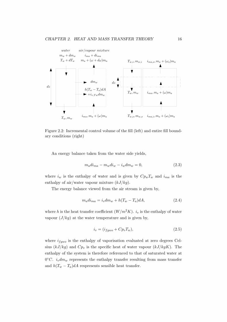
2.6 Poppe model
Poppe [10] was among the first researchers to publish a ’complete model’
to simulate cooling tower performance. These equations are derived in a
manner similar to the Merkel equation but without the additional assump-
tions. The Poppe equations are derived in Appendix A. The resulting three
equations are given below in Eqns. 2.8, 2.9 and 2.10,
dω
dTw=
[Cpw(mw/ma) · (ω′′
(Tw) − ω)
iv · (ω′′
(Tw)− ω) + LefCpma(Tw − Ta) − CpwTw(ω′′
(Tw)− ω)
],
(2.8)
dima
dTw= Cpw
mw
ma
[1 +
(CpwTw(ω′′
(Tw) − ω)
)/(iv · (ω′′
(Tw) − ω) +
LefCpma(Tw − Ta) − CpwTw(ω′′
(Tw) − ω)
)], (2.9)

CHAPTER 2. HEAT AND MASS TRANSFER THEORY 21
dMep
dTw=
Cpw
iv · (ω′′
(Tw) − ω) + LefCpma(Tw − Ta) − CpwTw(ω′′
(Tw) − ω).
(2.10)
Mep in Eqn. 2.10, is the Merkel number for the Poppe equations. These
equations are modified under saturation conditions. For details see Ap-
pendix A. To solve the three equations Runge-Kutta numerical integration
can be used. The form of the equations means that process is highly it-
erative however. In fill performance tests, the water outlet temperature is
known so the equations are numerically integrated to find the Poppe Merkel
number. The water outlet mass flow rate is not known a-priori or measured
directly so the equations are solved iteratively until the guessed water mass
flow rate equals the final calculated value within the specified tolerance. To
improve the system, the water mass flow rate at any point in the fill can be
written in terms of the inlet mass flow rate, the current air specific humidity
and the inlet air mass flow rate [10, 55]:
mratio =mw
ma=
mw,i
ma
(1 − ma
mw,i(ωo − ω)
). (2.11)
This allows the outlet humidity to be guessed instead of the outlet water
mass flow rate. The air outlet specific humidity can be initially guessed by
finding the saturation specific humidity at the average of the air and water
inlet temperatures. In this way the equations are solved iteratively until
the guessed outlet air specific humidity equals the calculated value within a
tolerance δωo . The process is given in Fig. 2.4 (a).
In tower performance calculations the Poppe Merkel number is known
but the water outlet temperature and mass flow rate are not. In a similar
manner, both the water temperature (Tw,o) and the air specific humidity are
found by repetitive iteration until the guessed specific humidity is within a
tolerance δωo of the calculated value and the calculated Merkel number is
within a tolerance δMep of the known value.
The air enthalpy, air humidity and the water temperature are known at
each step. These can be used to determine the free air stream properties
and the properties of the vapour film at the water surface. The switch
between the unsaturated and saturated Poppe equations is based on the

CHAPTER 2. HEAT AND MASS TRANSFER THEORY 22
Goal: Calculate Mep with known Tw,o
1 Measure mw, Ta,i, Tw,i, ma, Tw,o, δωo
2 n = 13 Guess w′n
o
4 While δ′nωo> δωo
5 n = n + 16 ω′n
o = ω′n−1o
7 Numerically integrate the Poppe equations (A.22,A.24, A.28) between Tw,o and Tw,i to findMe′np and ω′n
o . If the air becomes saturated
then switch to Eqns. A.31, A.32, A.338 Compare calculated ω′n+1
o to the initial guessedvalue specified in step (6), δ′nωo
= ω′no − ω′n−1
o
9 Mep = Me′np and ωo = ω′no
10 END
(a)
Goal: Calculate Tw,o with known Mep
1 Specify mw, Ta,i, Tw,i, ma, Mep, δMep , δω
2 n = 1,m = 13 Guess ωn
o and T ′mw,o
4 While δ′nωo> δωo
5 n = n + 16 ω′n
o = ω′n−1o
7 m = 18 While δ′nMep
> δMep
9 m = m + 110 Estimate new water outlet temperature using :
T ′mw,o = T ′m−1
w,o − δ′m−1Mep
(T ′m−1w,o − T ′m−2
w,o )/(δ′m−1Mep
− δ′m−2Mep
)
11 Numerically integrate the Poppe equations (A.22,A.24, A.28) between T ′m
w,o and Tw,i to find
Me′np and ω′no . If the air becomes saturated
then switch to Eqns. A.31, A.32, A.3312 Compare calculated Me′mp to the value specified
in step (1), δ′mMep= Mep − Me′mp
13 Compare calculated ω′no to the initial guessed
value specified in step (6), δ′nwo= ω′n
o − ω′n−1o
14 Tw,o = T ′mw,o and ωo = ω′n
o
15 END
(b)
Figure 2.4: Poppe solver procedure in fill test procedure (a) and subsequenttower performance evaluation (b)
CHAPTER 2. HEAT AND MASS TRANSFER THEORY 23
relative humidity:
RH =Pv
Psat. (2.12)
Further details on these methods can be found in Kroger [1] and Klop-
pers [3]. The specific heats and other flow properties are evaluated using
correlations taken from Kroger [1] (see Appendix B ).
2.7 Other models
The NTU model developed by Jaber [1, 11] employs the same assumptions as
Merkel’s method so is no more accurate. It was originally devised to create
a method more closely related to heat exchanger design methods. Other
models have appeared in literature but these are generally very similar to the
Poppe and Merkel models and have not been widely adopted [14, 53, 56, 60].
2.8 Discussion
Neither the Poppe or the Merkel model are calibrated to give the accurate air
temperature or humidity at the exit of the fill. Both methods are calibrated
to only find the water outlet temperature. Because the Poppe method is
more rigorous however, the outlet air temperature and humidity are closer
to the true value. Kloppers [3] presents the Merkel and Poppe model pre-
dictions of air outlet temperature against experimental results and finds the
Poppe model an excellent fit while the Merkel predictions were conservative
(lower). This difference is important for NDWCTs where the tower draft
is a function of the air exit condition. The Merkel model requires that the
exit condition be estimated from the calculated air enthalpy, assuming the
air is saturated. For the range of conditions that will be encountered in this
study, the air is always saturated or supersaturated at the fill outlet.
Kloppers [3] conducts the most in depth comparison of the Merkel, Poppe
and NTU methods to date under a range of conditions. The author finds
that if only the water outlet temperature is of interest then the Merkel
model is acceptable as the results are very similar to the Poppe method.
The author stresses that it is imperative that the fill is tested and transfer
coefficient correlations developed at conditions as close as possible to the
design conditions.

CHAPTER 2. HEAT AND MASS TRANSFER THEORY 24
2.9 Empirical transfer coefficients
Fill thermal performance is described by the Merkel number or transfer
coefficient. These are derived from laboratory fill tests. The coefficients are
reported as empirical correlations as a function of the dependent variables,
usually the air and water mass flow rate per unit area (also termed mass
fluxes or mass velocities, Ga and Gw).
Kloppers and Kroger [1, 3] give a detailed account of fill test procedures.
In these tests, the water flow rate and air flow rate are usually controlled.
The water inlet and outlet temperatures are measured as is the air inlet
temperature. The Merkel or Poppe method can then be used to find the
Merkel (or Poppe Merkel) number for the fill. The data is correlated to give
an empirical equation of the Merkel number as a function of the dependent
variables. The functionality included in this correlation is very important to
the generality of the model and accuracy when designing the cooling tower.
A number of different formats have appeared in literature. Lowe [7]
presented coefficients in the form of Eqn. 2.13 while Kroger [1] presents a
range of coefficients from a number of sources using:
Me/Lfi =hmA
mw= c1(
Gw
Ga)c2, (2.13)
Me/Lfi =hmA
mw= c1G
c2w Gc3
a , (2.14)
where c1, c2 and c3 are constants found from experiment and Lfi is the
depth of the fill. For a full discussion see [1, 3].
Recently Kloppers and Kroger [3, 61] have proposed the following form:
Me/Lfi =hmA
mw= c1G
c2w Gc3
a + c4Gc5w Gc6
a . (2.15)
The authors found that this fitted the experimental data more closely than
Eqn. 2.14. The authors provided empirical correlations for the Merkel,
Poppe and NTU methods and the complete set of experimental data in [3],
for three fill types. In addition the authors tested the functional dependence
of the fill Merkel number to air temperature, fill depth and water inlet
temperature. The authors found that the Merkel number is not dependent
on air inlet temperature or wet bulb temperature but is a function of fill

CHAPTER 2. HEAT AND MASS TRANSFER THEORY 25
depth as given in,
Me/Lfi =hmA
mw= c1G
c2w Gc3
a Lc4fi. (2.16)
The authors noted that during the tests the water temperature was not
constant and found the exponent on Twi in Eqn. 2.17 to be significant
implying the functional dependence of the system upon it:
Me/Lfi =hmA
mw= c1G
c2w Gc3
a Lc4fiT
c5wi. (2.17)
In this study all transfer coefficients are taken from Kloppers thesis [3]
or interpreted from the data in the same work.

Chapter 3
Computational Fluid
Dynamics
3.1 Introduction
This chapter is a brief overview of computational fluid dynamics (CFD) and
the numerical methods employed in FLUENT [40], a general purpose com-
mercial CFD package widely used in engineering applications. This package
has been employed in this study to develop a two dimensional axisymmetric
steady state simulation of a NDWCT. The governing equations and meth-
ods employed in this model are presented here with some brief discussion.
A more detailed description of numerical methods and CFD is contained in
many standard texts [62, 63].
3.2 Computational fluid dynamics
The governing equations for incompressible steady fluid flow can be written
in general form as:
∇ · (ρuφ − Γφ∇φ) = Sφ, (3.1)
where ρ is the air density (kg/m3), u is the fluid velocity (m/s), φ is the
flow variable (u, v,w, k, ǫ, T, ω) and Γφ is the diffusion coefficient for φ and
Sφ the source term. These equations can be expanded into the individual
momentum and transport equations which, together with the continuity
equation give the Navier-Stokes Equations. These equations can be solved
numerically enabling fluid flow to be simulated forming the basis for CFD.
26

CHAPTER 3. COMPUTATIONAL FLUID DYNAMICS 27
In the following sections these equations are introduced and discussed.
3.3 Continuity and momentum equations
The continuity equation for conservation of mass in Cartesian coordinates
for transient flow can be given as,
∂ρ
∂t+ ∇ · (ρ~v) = Sm, (3.2)
where Sm is the mass source term. The steady equation is obtained by
simply neglecting the transient terms, ∂∂t , from the left hand side.
The equation for conservation of momentum can be written as,
∂
∂t(ρui) +
∂
∂xj(ρuiuj) = − ∂p
∂xi+
∂
∂xj
[µ
(∂ui
∂xj+
∂uj
∂xi
)]+ S, (3.3)
where S is now a source term for momentum. The source term for buoyancy
can be written as,
Sb = (ρ − ρref )g. (3.4)
The transport equation for a scalar φ can be written as:
∂
∂t(ρφ) +
∂
∂xj(ρφuj) =
∂
∂xj
[ρΓ
(∂φ
∂xj
)]+ Sφ. (3.5)
3.4 Turbulence modelling
The above equations are the Navier-Stokes equations. These represent all
the scales of fluid motion. Our ability to solve these equations is limited
by the computational resources available. Many flows in engineering are
highly turbulent and so resolving all the scales explicitly using direct nu-
merical simulation (DNS) is too computationally intensive, requiring very
fine discretisation of the above equations. Instead, turbulence models are
employed which reduce the computational work load by introducing sim-
plifying assumptions and representing some of the scales of motion with
additional equations.
The selection of a simulation approach/model depends on the application
and type of result required. One approach is to use a large eddy simulation
(LES) where the flow field is filtered and the smallest scales of motion are

CHAPTER 3. COMPUTATIONAL FLUID DYNAMICS 28
modelled with a sub-filter scale (SFS) model and the large scales are solved
directly. Because only the small scales are modelled, the simulations retain
a high degree of accuracy. Additionally, because the smallest scales of tur-
bulence are expected to be more isotropic and homogeneous than the large
scales, the SFS scale models should be more universal than other modelling
approaches such as the RANS approach described below. LES methods are
time dependent and fully three dimensional. Since they are required to solve
all but the smallest scales of motion, they still tend to be very computation-
ally intensive and are at present limited to simulating low Reynolds number
flows. Such an approach is necessary for example when accurate prediction
of the stresses in the flow and mixing is required.
Another approach is to solve the Reynolds Averaged Navier-Stokes (RANS)
equations. In this method, the time averaged Navier Stokes equations are
solved to yield the mean velocity field with all the turbulent stresses mod-
elled using some additional set of equations. The steady state RANS equa-
tions can be solved very economically for very high Reynolds number flows
and are at present the only practical avenue available for solving problems
such as the flow through a NDWCT because of the size of the simulation in
terms of computational load. The difficulty can be seen by examining the
characteristic parameters for the flow in a NDWCT, which are the Reynolds
number, Re = V Lν , and the Grashof number, Gr = gL3∆ρ/ρo
ν2 . In these equa-
tions, the characteristic length scale used is the tower height (L = 131m), V
is the air velocity above the fill, ∆ρ is the density difference between the air
inside the tower and the ambient air ρo. Typical values for a simulation in
this study are V ∼ 2.0 m/s and ∆ρ/ρo ∼ 0.12. These values are presented
in latter chapters. This gives a Reynolds number of ∼ 1.7 × 10⁷ and the
Grashof number of ∼ 8.8 × 10¹³. Both these parameters give an indication
of how difficult these simulations are. The flow is very turbulent and the
buoyancy forces as indicated by the Grashof number are very strong.
In this study, a RANS model has been used for the simulations of tur-
bulent flow in a NDWCT. A more detailed discussion of this approach is
contained in section 3.5. In addition however, in this thesis some contribu-
tion is made to testing a range of LES models. This work is presented in
Chapter 4.

CHAPTER 3. COMPUTATIONAL FLUID DYNAMICS 29
3.5 RANS turbulence modelling
The RANS equations are derived by first decomposing the velocity and
pressure into its mean and fluctuating components as shown in Eqn. 3.6:
u = U + u′, (3.6)
where U is the mean velocity component and u′ is the fluctuating component.
Substituting Eqn. 3.6 into the momentum equation yields the Reynolds
averaged momentum equation (in Cartesian coordinates) (Eqn. 3.7),
∂
∂t(ρUi) +
∂
∂xj(ρUiUj) = − ∂p
∂xi+
∂
∂xj
[µ
(∂Ui
∂xj+
∂Uj
∂xi
)]
+∂
∂xj(−ρu′
iu′
j). (3.7)
The terms −ρu′
iu′
j are the unresolved turbulent Reynolds stresses. A
popular approach to modelling these terms is to use the eddy viscosity con-
cept. In this approach, the turbulence is represented as additional mixing
or diffusion in the model, so in the momentum equation the effective total
viscosity is given as a sum of the molecular viscosity and the artificial tur-
bulent viscosity µeff = µ + µt. This is introduced in the model following
the gradient diffusion hypothesis. In this theory, the Reynolds stress or tur-
bulence scalar flux is related to the turbulent viscosity/diffusivity and the
mean scalar gradient as given in Eqn. 3.8 and Eqn. 3.9 respectively,
−ρu′
iu′
j = µt
(∂ui
∂xj+
∂uj
∂xi
), (3.8)
−ρφ′u′
j = ρµt
Sct
(∂φ
∂xj
). (3.9)
A more comprehensive discussion is contained in Pope [64]. Generally,
the eddy viscosity hypothesis is most reasonable in flows characterised by
simple shear, where the mean velocity gradients change slowly.
In order for the model to be closed, a prescription to describe the eddy
viscosity, µt, must be provided. There are numerous turbulent-viscosity
models. They can be classified into the number of equations they are com-
prised of. In one equation models or algebraic models, a characteristic turbu-
lent length scale must be specified a-priori. Two-equation turbulent-kinetic-

CHAPTER 3. COMPUTATIONAL FLUID DYNAMICS 30
energy models such as the k − ǫ or k − ω models are slightly more complex.
In these models, the transport equations for turbulent kinetic energy and
dissipation are solved which together provide the characteristic turbulent
length scales. These are termed ’complete’ models as the length scales do
not need to be specified a-priori. These models are very empirical however
and are usually tuned to a specific flow. Here the standard k− ǫ turbulence
model is examined in more detail as it has been employed for all NDWCT
simulations in this study.
3.5.1 k − ǫ transport equations
The transport equations for the turbulence kinetic energy, k, and the rate
of dissipation, ǫ, are given in Eqns. 3.10 and 3.11 respectively:
∂
∂t(ρk) +
∂
∂xi(ρkui) =
∂
∂xj
[(µ +
µt
σk
)∂k
∂xj
]
+ Gk + Gb − ρǫ + Sk, (3.10)
∂
∂t(ρǫ) +
∂
∂xi(ρǫui) =
∂
∂xj
[(µ +
µt
σǫ
)∂ǫ
∂xj
]
+ C1ǫǫ
k(Gk + C3ǫGb) − C2ǫρ
ǫ2
k+ Sǫ, (3.11)
where Sk and Sǫ are the source terms. All model coefficients are given in
Table 3.1. The eddy viscosity µt, is found from Eqn. 3.12:
µt = ρCµk2
ǫ. (3.12)
The production of turbulence kinetic energy, denoted by the term Gk is
given in Eqn. 3.13:
Gk = −ρu′
iu′
j
∂uj
∂xi
= µtS2, (3.13)
where S is defined as S ≡√
2SijSij . Gb represents the generation of turbu-

CHAPTER 3. COMPUTATIONAL FLUID DYNAMICS 31
Table 3.1: Model coefficients for k − ǫ turbulence model
C1ǫ C2ǫ Cµ σk σǫ
1.44 1.92 0.09 1.0 1.3
lence due to buoyancy and is given in Eqn. 3.14:
Gb = βgiµt
Prt
∂T
∂xi, (3.14)
where gi is the component of the gravitational vector in the ith direction,
the turbulent Prandtl number, Prt, is 0.85 and the coefficient of thermal
expansion is defined as β = −1ρ
(∂ρ∂T
)p.
The effect of buoyancy on turbulent dissipation is specified through C3ǫ
as given in Eqn. 3.15:
C3ǫ = tanh∣∣∣vu
∣∣∣ , (3.15)
where v is the velocity aligned with the gravitational vector and u is the
component perpendicular to v.
3.5.2 Heat and mass transfer modelling
The transport equation for energy can be written as Eqn. 3.16:
∂
∂t(ρE) +
∂
∂xi[ui(ρE + p)] =
∂
∂xj
(keff
∂T
∂xj
)+ Sh, (3.16)
where E is the total energy, keff is the effective thermal conductivity given
by Eqn. 3.17 and k is the thermal conductivity,
keff = k +cpµt
Prt. (3.17)
The turbulent mass transport equation (Eqn. 3.18) is similar. The tur-
bulent Prandtl number (Prt) is replaced with the turbulent Schmidt number
(Sct) in Eqn. 3.17 to give the turbulent diffusion coefficient, Γt = µt
Sctand
the effective diffusion coefficient, Γeff = Γφ + Γt:
∂
∂t(φ) +
∂
∂xi[ui(φ)] =
∂
∂xj
(Γeff
∂φ
∂xj
)+ Sφ. (3.18)

CHAPTER 3. COMPUTATIONAL FLUID DYNAMICS 32
3.6 Axisymmetric equations
In this study, an axisymmetric geometry has been employed. In this case, the
above equations in Cartesian coordinates are transformed to the following
steady axisymmetric equations:
Continuity equation:
1
r
∂
∂r(rρvr) +
∂
∂x(ρvx) = Sm (3.19)
Axial momentum equation:
1
r
∂
∂x(rρvxvx) +
1
r
∂
∂r(rρvrvx) = −∂p
∂x+
1
r
∂
∂x
[rµeff
(2∂vx
∂x
)]
+1
r
∂
∂r
[rµeff
(∂vx
∂r+
∂vr
∂x
)]
+ Sx + (ρ − ρref )g
(3.20)
Radial momentum equation:
1
r
∂
∂x(rρvxvr) +
1
r
∂
∂r(rρvrvr) = −∂p
∂r+
1
r
∂
∂x
[rµeff
(∂vr
∂x+
∂vx
∂r
)]
+1
r
∂
∂r
[rµeff
(2∂vr
∂r
)]
− 2µeffvr
r2+ Sr
(3.21)
Generic scalar transport equation:
1
r
∂
∂x(rρvxφ) +
1
r
∂
∂r(rρvrφ) =
∂
∂x
[Γeff
σ
(∂φ
∂x
)]
+1
r
∂
∂r
[rΓeff
σ
(∂φ
∂r
)]+ Sφ
(3.22)

CHAPTER 3. COMPUTATIONAL FLUID DYNAMICS 33
Turbulent kinetic energy:
1
r
∂
∂x(rρkvx) +
1
r
∂
∂r(rρkvr) =
1
r
∂
∂x
[r
(µ +
µt
σk
)∂k
∂x
]
+1
r
∂
∂r
[r
(µ +
µt
σk
)∂k
∂r
]
+ µt
[2
(∂ux
∂x
)2
+
(∂vr
∂r
)2
+
(∂vr
∂x+
∂vr
∂r
)2
+ 2
(vx
r
)2]
+ Gb − ρǫ + Sk
(3.23)
Dissipation of turbulent kinetic energy:
1
r
∂
∂x(rρǫvx) +
1
r
∂
∂r(rρǫvr) =
1
r
∂
∂x
[r
(µ +
µt
σǫ
)∂ǫ
∂x
]
+1
r
∂
∂r
[r
(µ +
µt
σǫ
)∂ǫ
∂r
]
+ µtC1ǫǫ
k
([2
(∂vx
∂x
)2
+ 2
(∂vr
∂r
)2
+
(∂vx
∂r+
∂vr
∂x
)2
+
(vr
r
)2]+ C3ǫGb
)− C2ǫρ
ǫ2
k+ Sǫ
(3.24)
3.7 Numerical solution procedure
To solve the above set of equations, the computational domain is discretised
into a number of finite cells to form a mesh or grid as depicted in Fig.
3.1. The above equations are discretised onto this grid and written into an
algebraic set of linear equations which can be solved. There are a wide range
of numerical solution procedures that can be used to solve these equations.
In this section, the methods used in this study are briefly described.

CHAPTER 3. COMPUTATIONAL FLUID DYNAMICS 34
In FLUENT, the finite volume form is used for this discretisation. In
this form the generic scalar transport equation can be written as:
Nfaces∑
f
ρf~vfφf · ~Af =
Nfaces∑
f
Γφ (∇φ)n · ~Af + Sφ V, (3.25)
where Nfaces is the number of faces enclosing cell, φf is the value of φ ad-
vected through face f , ρf~vf · ~Af is the mass flux through the face, ~Af area
of the face, (∇φ)n is the magnitude of ∇φ normal to face f and V is the
cell volume.
FLUENT uses a collocated scheme whereby the pressure and the velocity
components are stored at the cell centres (Fig. 3.1). The face values used in
the advective terms are interpolated from the cell centres using an upwind
differencing scheme which is second order accurate. The face value, φf , is
calculated using:
φf = φ + ∇φ · ∆~s, (3.26)
where φ and ∇φ are the cell-centred value and its gradient in the upstream
cell respectively, and ∆~s is the displacement vector from the upstream cell
centroid to the face centroid. The gradient ∇φ is found using:
∇φ =1
V
Nfaces∑
f
φf~A, (3.27)
where φf are computed by averaging φ from the two cells adjacent to the
face. FLUENT applies a flux limiter to the gradient [40]. The diffusion
terms (∑Nfaces
f Γφ (∇φ)n· ~Af ), are discretised using central differencing which
is second order accurate.
The linearised system of equations is then solved using a Gauss-Seidel
linear equation solver used together with an algebraic multigrid method.
The pressure is coupled with the velocity using the SIMPLE algorithm [62,
63], with Rhie and Chow interpolation of the cell centre velocities onto the
cell faces [65]. In this scheme the momentum equations are first solved with
the guessed pressure p∗, resulting in an estimate for the velocity field, which
is in general not divergence free. The pressure and velocity fields are then

CHAPTER 3. COMPUTATIONAL FLUID DYNAMICS 35
φW φE
φN
φP
φS
xj xj+1
yj
yj+1
Figure 3.1: Flow variables stored on collocated grid, with scalar and vectorquantities stored at cell centres
corrected to ensure they satisfy the discrete continuity equation:
Nfaces∑
f
ρvnAf = 0, (3.28)
where vn is the normal velocity through face f . The pressure correction
equation is constructed by substituting a re-arrangement of the momentum
equation into the continuity equation, yielding a Poisson equation for the
pressure. The pressure correction equation is solved to find the correction
to the pressure, p′. This is then used to correct the velocity field. These
methods are standard and the reader is referred to standard texts such
as [62, 63] for further details.

Chapter 4
Large Eddy Simulation of
Heat Transport in Turbulent
Channel Flow
4.1 Introduction
It is well known the LES can provide more accurate and detailed simulations
of turbulent flow than the RANS models [64]. The flow in a NDWCT is
highly turbulent and very complex, with strong density gradients, multi-
phase flow and combined heat and mass transfer. The mean air flow should
be well predicted by the k − ǫ RANS model but there are many areas in
which RANS models are limited. LES is much more suited to examining
the effect of turbulence on droplet flow, or resolving the flow through the
fill with the highly complex air/water interaction or simulating the effect of
cold air inflow into the tower outlet. While these issues are not examined in
this thesis, in the future, LES is a possible approach to take for such studies.
However, there is still much development required before LES models can
be applied with confidence to situations in which they have not been tested
first. The propose of this chapter is to examine the some recently developed
LES methods and apply them to a flow topical to that in a NDWCT. The
test case chosen is a simulation of turbulent channel flow with transport of
a passive scalar. This case is chosen because DNS benchmark solutions are
readily available and the mechanisms behind turbulent transport of a scalar
is important to flow in a NDWCT. The main contribution of the work in this
36

CHAPTER 4. LES OF SCALAR TRANSPORT 37
chapter is to further the understanding of several new LES models and their
suitability for simulations of scalar transport. These methods have not been
implemented in any of the NDWCT investigations in this thesis because of
computational limitations, so this chapter is not essential for the reader to
have an understanding of the chapters that follow.
This chapter is laid out as follows. In sections 4.2 - 4.4 background
on recent LES developments is presented and motivation for this work is
discussed. In section 4.5, the governing equations, LES models and the test
case are described. The numerical model is described in section 4.6 and the
simulation results are presented in section 4.7. Conclusions are drawn in
section 4.8.
4.2 Background
In a large eddy simulation, a low pass filter is applied to the governing
equations, separating the large resolved scales from the unresolved sub-
filter-scales (SFS). In most LES simulations the computational grid and
the discretisation of the equations provide the implicit filter, where the filter
width is taken as the grid dimension [66]. This implicit filtering operation
is denoted here by the operator (·), and is applied to the conservation, mo-
mentum and generic transport equations as follows,
∂u
∂xj= 0, (4.1)
∂u
∂t+
∂(uiuj)
∂xj= − ∂p
∂xi+ ν
∂2ui
∂xj∂xj− ∂τij
∂xj, (4.2)
∂φ
∂t+
∂˜(φuj)
∂xj= α
∂2φ
∂xj∂xj− ∂γ
∂xj. (4.3)
The SFS stresses are given by τij = (uiuj) − (uiuj) and the SFS heat flux
term is defined as γ = (φuj) − ˜(φuj). In LES, a SFS model is specified to
represent the unknown terms τij and γ.
There are several difficulties however with the implicit nature of the fil-
ter in these simulations. Firstly, the exact nature of the implicit filter is
unknown and is different for each term, making SFS modelling difficult.
Secondly, unless high order finite differencing schemes are used, the numer-
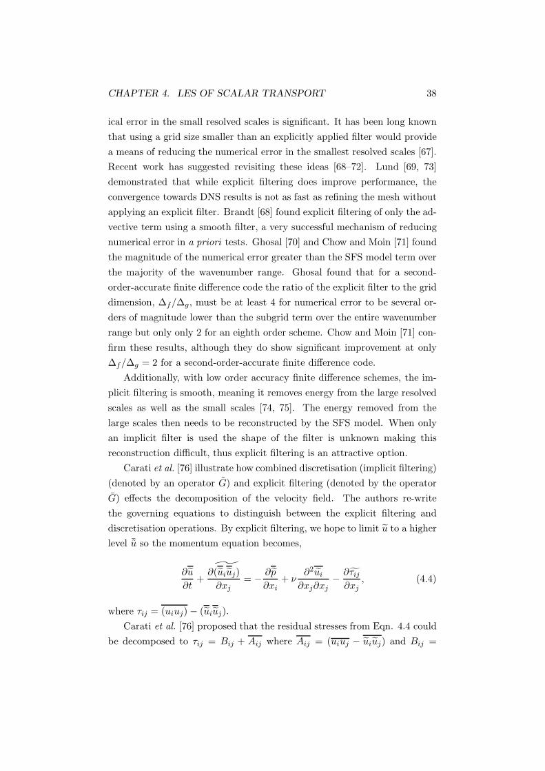
CHAPTER 4. LES OF SCALAR TRANSPORT 38
ical error in the small resolved scales is significant. It has been long known
that using a grid size smaller than an explicitly applied filter would provide
a means of reducing the numerical error in the smallest resolved scales [67].
Recent work has suggested revisiting these ideas [68–72]. Lund [69, 73]
demonstrated that while explicit filtering does improve performance, the
convergence towards DNS results is not as fast as refining the mesh without
applying an explicit filter. Brandt [68] found explicit filtering of only the ad-
vective term using a smooth filter, a very successful mechanism of reducing
numerical error in a priori tests. Ghosal [70] and Chow and Moin [71] found
the magnitude of the numerical error greater than the SFS model term over
the majority of the wavenumber range. Ghosal found that for a second-
order-accurate finite difference code the ratio of the explicit filter to the grid
dimension, ∆f/∆g, must be at least 4 for numerical error to be several or-
ders of magnitude lower than the subgrid term over the entire wavenumber
range but only only 2 for an eighth order scheme. Chow and Moin [71] con-
firm these results, although they do show significant improvement at only
∆f/∆g = 2 for a second-order-accurate finite difference code.
Additionally, with low order accuracy finite difference schemes, the im-
plicit filtering is smooth, meaning it removes energy from the large resolved
scales as well as the small scales [74, 75]. The energy removed from the
large scales then needs to be reconstructed by the SFS model. When only
an implicit filter is used the shape of the filter is unknown making this
reconstruction difficult, thus explicit filtering is an attractive option.
Carati et al. [76] illustrate how combined discretisation (implicit filtering)
(denoted by an operator G) and explicit filtering (denoted by the operator
G) effects the decomposition of the velocity field. The authors re-write
the governing equations to distinguish between the explicit filtering and
discretisation operations. By explicit filtering, we hope to limit u to a higher
level ¯u so the momentum equation becomes,
∂u
∂t+
∂ ˜(uiuj)
∂xj= − ∂p
∂xi+ ν
∂2ui
∂xj∂xj− ∂τij
∂xj, (4.4)
where τij = (uiuj) − (uiuj).
Carati et al. [76] proposed that the residual stresses from Eqn. 4.4 could
be decomposed to τij = Bij + Aij where Aij = (uiuj − uiuj) and Bij =

CHAPTER 4. LES OF SCALAR TRANSPORT 39
(uiuj − ¯ui¯uj). Aij is the sub grid scale (SGS) stress that cannot be captured
by the grid or implicit filter. Bij represents the interactions of the resolved
scales (¯u) and SFS motions (u− ¯u), which are the filtered scales that are still
supported by the grid. The notation of Chow et al. [77] is used where, Aij =
τSGS is the sub grid scale model term and Bij = τRSFS are the reconstructed
subfilter scale terms. The total model becomes τ = τSGS + τRSFS.
In τRSFS, the variable ui is not available, because the solution is now
limited to ¯u. An approximation to this term, u⋆i , can be made through
an approximate inverse filtering procedure (using the explicit filter G) from
expansion of the series in Eqn. 4.5 to reconstruction level N [78, 79].
ui ≈ u⋆i =
N∑
n
(I − G)nui (4.5)
In all these simulations, the application of the explicit filter G, only occurs in
the SFS models. The filter is never applied to the velocity field itself [77, 80].
The solution itself is limited to the ¯G level because in these models, the
τRSFS term partially cancels with the advective term and is equivalent to
explicit filtering of the advective term itself. This was shown by Lund [69, 73]
to be an effective method of filtering the solution.
The work in this chapter is specifically aimed at examining the perfor-
mance of explicit filtering and the effect of reconstruction on the transport
of a passive scalar. Of interest is determining both the effect of the velocity
field on scalar transport and the effect of the closure of the SFS heat flux
itself. In the next two sections, a range of SFS models are introduced within
the framework outlined above.
4.3 Sub-filter-scale stress models
Among the first models proposed was the Smagorinsky model [64], which is
a linear eddy viscosity model where the residual stress is proportional to the
filtered rate of strain, so τij = τSGS = −2cs(∆)2|S|Sij . No explicit filtering
is employed in this model so the τRSFS = 0. The model coefficient, cs is a
constant, Sij = 12( ∂ui
∂xj+
∂uj
∂xi) is the strain rate and |S| = (2Sij Sij)
1/2 is the
resolved strain rate tensor. This model is purely dissipative, where energy
is only transfered from the resolved scales to the SFS. A major advance was
proposed by Germano et al. [81], where the model coefficient is calculated

CHAPTER 4. LES OF SCALAR TRANSPORT 40
dynamically by comparing the resolved scales at two filter levels. This al-
lows the model coefficient to vary throughout the flow and correctly gives
coefficient at the wall, eliminating the need for wall functions, provided the
flow is sufficiently well resolved.
Bardina et al. [82] proposed the ’scale-similarity model’ (SSM). In this
model the implicit filtered velocity (u), is approximated by the explicit fil-
tered velocity, ¯u. In this way u ≈ ¯u and reconstruction term, τRSFS, can be
written as τij = τRSFS = (¯ui¯uj)−(¯ui
¯uj). The term τSGS, is ignored however
and this model has been shown to provide insufficient damping [83]. This
was overcome by Zang et al. [84] who proposed the dynamic mixed model
(DMM) where the SFS stress is a linear combination of the SSM and the
DSM models and is given as,
τij = (¯ui¯uj) − (¯ui
¯uj) − 2(C∆)2| ¯S| ¯Sij . (4.6)
This model was later improved by Vreman et al. [83] and shown to give
very good results compared with the DSM and SSM. Sarghini et al. [85]
came to similar conclusions. This model has performed well in many test
cases and has been the subject of continued interest and development. In
a-priori tests, the mixed model shows stronger correlation with DNS re-
sults than models without the τRSFS term [86]. Winckelmans et al. [79]
formulated a dynamic reconstruction model (DRM) based on the explicit
filtering frame work they introduced. Gullbrand and Chow [80] imple-
mented a higher order version of the reconstruction model and found im-
proved performance over the DMM and DSM models in a turbulent channel
flow simulation. Gullbrand and Chow formulated the SFS stress as follows,
τRSFS = (u⋆i u
⋆j ) − (¯ui
¯uj) and τSGS = −2cs(∆)2| ¯S| ¯Sij so,
τij = (u⋆i u
⋆j ) − ( ¯ui
¯uj) − 2cs(∆)2| ¯S| ¯Sij. (4.7)
In this way, the model is simply a higher order version of the DMM, where
u in the τRSFS term is approximated by u⋆ instead of ¯u. Chow et al. [77]
applied the DRM to an atmospheric boundary layer simulation and found
improved performance compared with DSM and DMM models. The DRM
model is similar to the approximate deconvolution model of Stolz et al. [78].

CHAPTER 4. LES OF SCALAR TRANSPORT 41
4.4 Sub-filter-scale heat flux modelling
Much of the development in SFS heat flux models has followed directly from
models of the residual stress tensor in the momentum equations. The dy-
namic heat flux model proposed by Moin et al. [87] is based on the dynamic
Smagorinsky model of Germano et al. [81]. The SFS heat flux is modelled
using, γ = −cφ∆2|S|∂φxj
, where the model coefficient cφ is calculated dynam-
ically. This model was further developed by Wong and Lilly [88]. It has
since become the standard model to which all models are compared against.
It suffers from the same assumptions as the DSM model for momentum. It
assumes the SFS heat flux is aligned with the resolved temperature gradient
and is wholly dissipative.
Following this work a number of researchers have proposed non-linear
models for the SFS heat flux term, which removes the assumption of align-
ment with the resolved temperature gradient. Salvetti and Banerjee [86]
developed a dynamic two parameter model (DTM) which is similar to the
DMM model of Zhang et al. [84]. In a priori the authors found both the
DMM and the DTM models had a high degree of correlation with DNS data
for both heat flux and SFS stresses, but the DSM model performed more
poorly. Jimenez et al. [89] tested the DMM, the DTM and the DSM in a
mixing layer and found that the eddy diffusivity model works well, provided
the resolved velocity field is captured well. In a posteriori tests, the author
found comparable results when the DSM was used for modelling γ and the
DMM used for modelling τ and the DMM for γ and τ . The results were not
as good when the DSM model was used for modelling both γ and τ .
Peng and Davidson [90] developed a tensor diffusivity model which for-
mulates γj ∝ −Sij∂φ/∂xj . Yin et al. [91] applied this model in a simulation
of turbulent channel flow with buoyancy. The authors found better agree-
ment with DNS using the tensor diffusivity model for γ and a non linear
model for τ , than using the DSM for both γ and τ . Wang et al. [92] devel-
oped a tensorial diffusivity model which the authors demonstrate is a more
general case of the two coefficient dynamic mixed model of Sarghini et al..
The model showed slightly improved performance over the the DSM model
in a simulation of turbulent channel flow.
The reported good performance of the mixed models for both SFS resid-
ual stress and SFS heat flux is encouraging and suggests that the DRM,

CHAPTER 4. LES OF SCALAR TRANSPORT 42
which is a higher order version of the DMM, should also perform well. In
this study we compare the performance of the DRM, DMM and DSM mod-
els for both SFS heat flux and SFS stress in a simulation turbulent channel
flow with transport of a passive scalar. Two aspects in particular are of
interst. Firstly, how the closure of the SFS stress term τ effects both the
flow and the transport of the scalar and secondly, how the closure of the
SFS heat flux term γ performs. In this study we extend the DRM model to
model γ.
4.5 Governing equations
The models are tested in a fully developed turbulent channel flow simulation
between two parallel vertical walls as shown in Fig. 4.1. The streamwise (x)
and spanwise directions (z) have periodic boundaries while no slip boundary
conditions are used at the channel walls. The walls are at constant temper-
ature, TC and TH as shown in the figure. Buoyancy is not considered so
temperature becomes a passive scalar φ, which is non-dimensionalised by
temperature difference ∆T = TH − TC . The flow is driven by a constant
mean pressure gradient, which becomes unity when the flow variables are
non-dimensionalised by the wall friction velocity uτ =√
τw/ρ. The govern-
ing equations become,
∂u
∂t+
∂(uiuj)
∂xj= − ∂p
∂xi+
1
Reτ
∂2ui
∂xj∂xj(4.8)
where Reτ = δuτ /ν is the Reynolds number based on wall friction velocity,
and δ is the channel half width. The transport equation for the scalar φ is,
∂φ
∂t+
∂(φuj)
∂xj=
1
PrReτ
∂2φ
∂xj(4.9)
The simulation is based on the study of Kasagi and Iida [93] who provide
DNS results at Reτ = 150 with the Prandtl number, Pr = 0.71.
In this study two categories of SFS model are used, those with explicit
filtering and those without. In section 4.5.1 those models in which only
implicit filtering is used are described and in section 4.5.2 those models in
which explicit filtering is applied are described.

CHAPTER 4. LES OF SCALAR TRANSPORT 43
Lx
Ly
Lz
x
yz
THTC
Figure 4.1: Periodic channel flow configuration
4.5.1 Implicitly filtered SGS models
In this study the dynamic Smagorinsky model and a ’no-model’ simulation
are used. In both these cases, no explicit filtering is used so the momentum
and scalar transport equations become,
∂u
∂t+
∂(uiuj)
∂xj= − ∂p
∂xi+
1
Reτ
∂2ui
∂xj∂xj− ∂τij
∂xj, (4.10)
∂φ
∂t+
∂(φuj)
∂xj=
1
PrReτ
∂2φ
∂xj− ∂γ.
∂xj. (4.11)
where, τij = (uiuj) − (uiuj) and γ = (φuj) − ˜(φuj). A ’no-model’ or unre-
solved DNS simulation is one in which τij = 0 and γ = 0, so no model
is implemented. The dynamic Smagorinsky model is a variation of the
Smagorinsky model where τij = −2cs(∆)2|S|Sij and the model coefficient
and length scale cs(∆)2 are calculated dynamically [81]. This procedure is
described as follows.
A test filter, G, is applied to the filtered equations. When it is combined
with the implicit filter, the effective filter becomesG, and the equations are

CHAPTER 4. LES OF SCALAR TRANSPORT 44
written as follows,
∂u∂t
+∂
˜( uiuj)
∂xj= − ∂p
∂xi+
1
Reτ
∂2 ui
∂xj∂xj− ∂Tij
∂xj, (4.12)
where Tij =(uiuj)− ˜
(uiuj). Assuming similarity between the scales at grid
and test level, the model coefficient can be determined. The SFS stress at
the implicit filter level (τij) and the test level Tij are compared at the test
level following the Germano identity in Eqn 4.13,
Lij = Tij − τij (4.13)
= (uiuj) − (ˆuiˆuj).
The deviatoric subgrid stresses are formulated following the Smagorinsky
model and combined.
Tij −δij
3Tkk = −2cs
∆2
|S|Sij = −2csβij (4.14)
τij −δij
3τkk = −2cs∆
2|S|Sij = −2csαij (4.15)
Eqn 4.13 can be written as Eqn 4.16 with a single coefficient cs for both
levels assuming csαij = csαij .
Lij = −2csβij + 2csαij (4.16)
Now Eqn 4.16 can be written as Eqn 4.17 where Mij is given in Eqn 4.18
and the ratio σ = ∆/∆.
Lij = 2cs(∆)2Mij (4.17)
Mij = −σ2|S|Sij + |S|Sij (4.18)
The model coefficient is found with the error minimised using the least
squares approach in Eqn 4.19. The model coefficient, cs, is free to be positive
or negative and can cause the solution to become unstable. In most studies
it is stabilised by limiting the value of cs to be positive and averaging over
planes in which the flow is homogeneous. In their DMM, Zang et al. [84]
instead filtered the dynamic coefficient to the test level, a method akin
to a local averaging procedure. Gullbrand [94] found that local averaging
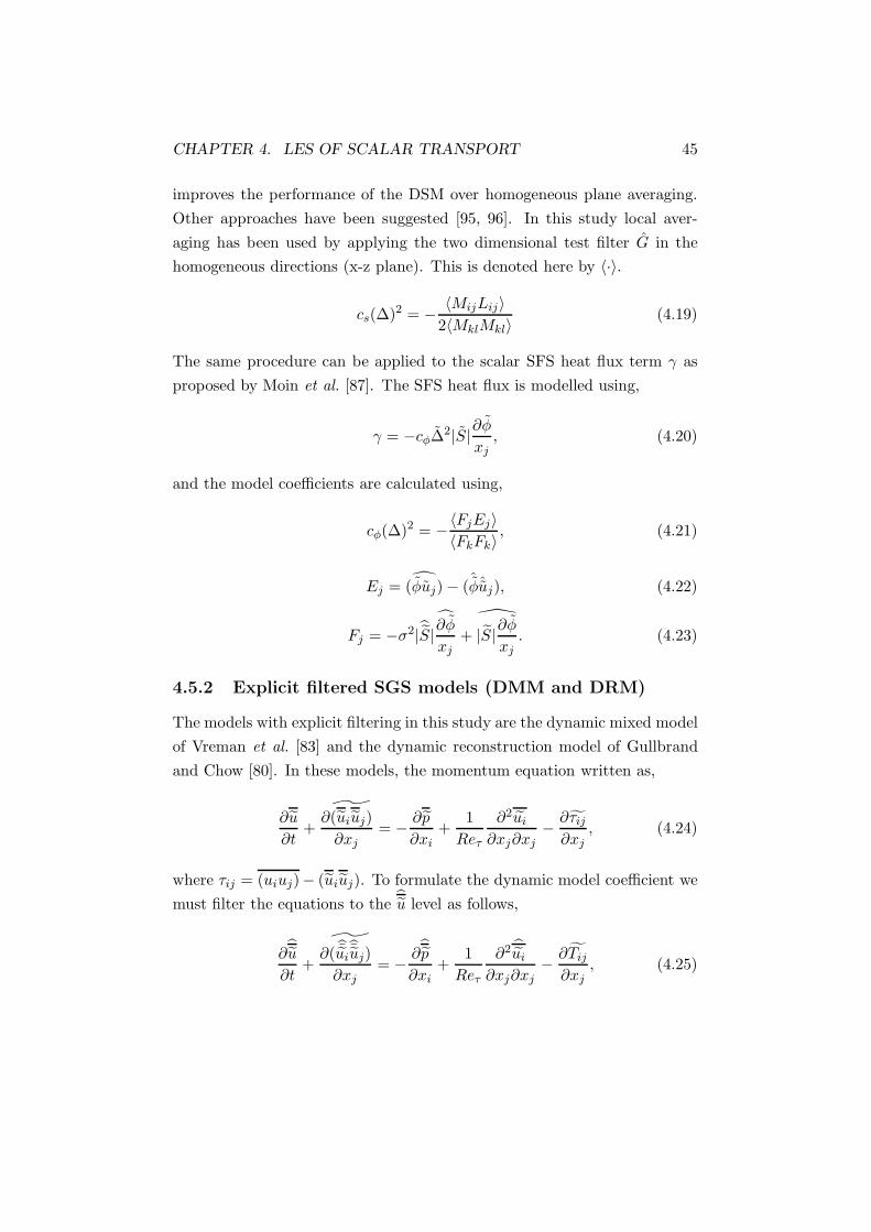
CHAPTER 4. LES OF SCALAR TRANSPORT 45
improves the performance of the DSM over homogeneous plane averaging.
Other approaches have been suggested [95, 96]. In this study local aver-
aging has been used by applying the two dimensional test filter G in the
homogeneous directions (x-z plane). This is denoted here by 〈·〉.
cs(∆)2 = − 〈MijLij〉2〈MklMkl〉
(4.19)
The same procedure can be applied to the scalar SFS heat flux term γ as
proposed by Moin et al. [87]. The SFS heat flux is modelled using,
γ = −cφ∆2|S|∂φ
xj, (4.20)
and the model coefficients are calculated using,
cφ(∆)2 = −〈FjEj〉〈FkFk〉
, (4.21)
Ej = (φuj) − (
ˆφˆuj), (4.22)
Fj = −σ2|S| ∂φ
xj+
|S|∂φ
xj. (4.23)
4.5.2 Explicit filtered SGS models (DMM and DRM)
The models with explicit filtering in this study are the dynamic mixed model
of Vreman et al. [83] and the dynamic reconstruction model of Gullbrand
and Chow [80]. In these models, the momentum equation written as,
∂u
∂t+
∂ ˜(uiuj)
∂xj= − ∂p
∂xi+
1
Reτ
∂2ui
∂xj∂xj− ∂τij
∂xj, (4.24)
where τij = (uiuj)− (uiuj). To formulate the dynamic model coefficient we
must filter the equations to the u level as follows,
∂u∂t
+∂
˜( uiuj)
∂xj= − ∂p
∂xi+
1
Reτ
∂2 ui
∂xj∂xj− ∂Tij
∂xj, (4.25)
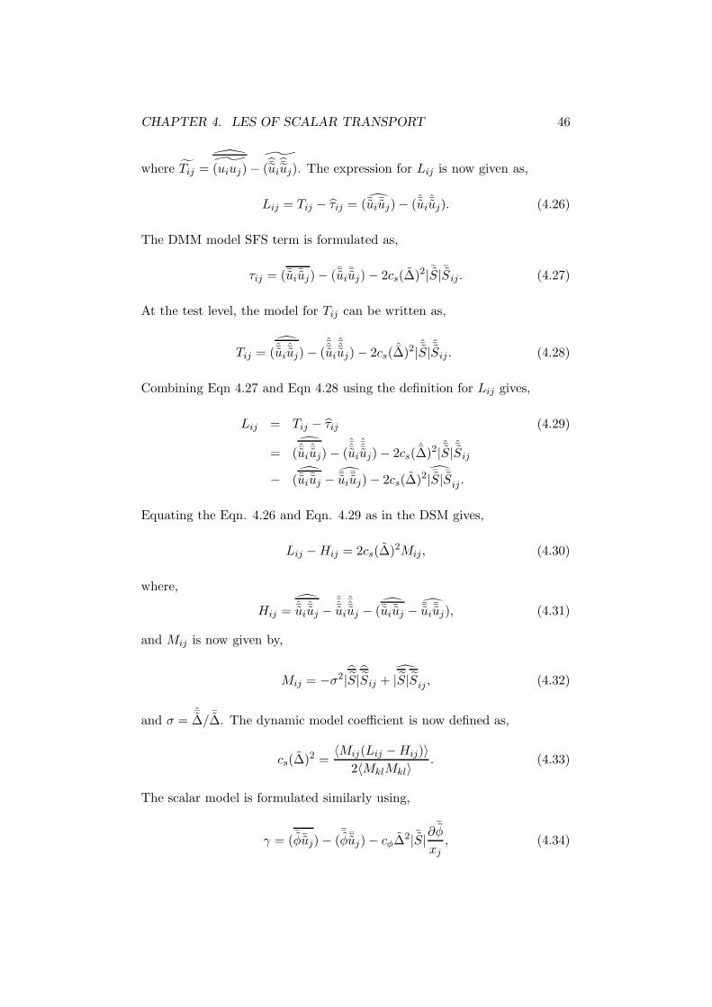
CHAPTER 4. LES OF SCALAR TRANSPORT 46
where Tij =(uiuj) −
˜(uiuj). The expression for Lij is now given as,
Lij = Tij − τij = ( ui¯uj) − (ˆui
ˆuj). (4.26)
The DMM model SFS term is formulated as,
τij = (¯ui¯uj) − (¯ui
¯uj) − 2cs(∆)2| ¯S| ¯Sij. (4.27)
At the test level, the model for Tij can be written as,
Tij = (ui
ˆuj) − (ˆ¯ui
ˆ¯uj) − 2cs(
ˆ∆)2| ˆS| ˆSij . (4.28)
Combining Eqn 4.27 and Eqn 4.28 using the definition for Lij gives,
Lij = Tij − τij (4.29)
= (ui
ˆuj) − (ˆ¯ui
ˆ¯uj) − 2cs(
ˆ∆)2| ˆS| ˆSij
− (ui
¯uj − ui
¯uj) − 2cs(∆)2 | ¯S| ¯Sij .
Equating the Eqn. 4.26 and Eqn. 4.29 as in the DSM gives,
Lij − Hij = 2cs(∆)2Mij , (4.30)
where,
Hij =ui
ˆuj −ˆ¯ui
ˆ¯uj − (
ui
¯uj − ui
¯uj), (4.31)
and Mij is now given by,
Mij = −σ2|S|Sij + |S|Sij , (4.32)
and σ =ˆ∆/ ¯∆. The dynamic model coefficient is now defined as,
cs(∆)2 =〈Mij(Lij − Hij)〉
2〈MklMkl〉. (4.33)
The scalar model is formulated similarly using,
γ = (¯φ¯uj) − (¯φ¯uj) − cφ∆2| ¯S|∂
¯φ
xj, (4.34)

CHAPTER 4. LES OF SCALAR TRANSPORT 47
and the model coefficients are calculated using,
cφ(∆)2 = −〈Fj(Ej − Gj)〉〈FkFk〉
, (4.35)
Gj =φˆuj −
ˆ¯φˆ¯uj − (
φ¯uj −
φ¯uj). (4.36)
In the DRM, the residual stress is constructed as:
τij = (u⋆i u
⋆j ) − ( ¯ui
¯uj) − 2cs(∆)2| ¯S| ¯Sij, (4.37)
where u⋆i is approximated using Eqn. 4.5. To satisfy similarity of the SFS
model at the test level, Tij must also be reconstructed to below the filter
level by the same degree. At the test level, reconstruction may be interpreted
as the inverse filtering of G. Assuming perfect reconstruction, this may be
represented by the removal of a filter G. In this case Tij may be written as
Eqn. 4.38.
Tij = (ui
¯uj) − (ˆui
ˆuj) − 2cs(
ˆ∆)2| ˆS| ˆSij (4.38)
When combined with the Germano identity following the same approach as
with the DMM, the model coefficient can be obtained as Eqn 4.39,
cs(¯∆)2 =
〈Mij(Lij − Hij)〉〈MklMkl〉
, (4.39)
where Hij = (ui
¯uj − (ˆui
ˆuj) − (u⋆
i u⋆j − ui
¯uj). The scalar SFS model is for-
mulated in a similar manner with,
γ = (φ⋆u⋆j ) − (¯φ ¯uj) − 2cs(∆)2| ¯S|∂
¯φ
xj. (4.40)
4.6 Channel flow simulation
The filtered equations are solved within a finite volume code on a staggered
Cartesian grid. Second-order-central differencing has been used for the spa-
tial discretisation on all terms in the momentum and pressure correction
equation. A fractional step method is used to advance the solution in time
with the advective terms integrated using a second order Adams-Bashforth
scheme and the diffusive terms using a second order accurate Crank-Nicolson

CHAPTER 4. LES OF SCALAR TRANSPORT 48
Table 4.1: Computational domainMesh x,y,z nx,ny,nz x+ y+
min y+max z+
A 15.7,2,6.3 70,74,70 33.6 0.6 8.7 13.5B 15.7,2,6.3 50,58,50 47.1 0.6 17.55 18.9
scheme. The code is described more completely in [97, 98].
Two computational grids have been used in this study as given in table
4.1. Constant linear stretching is used in the wall normal direction (y) while
a uniform mesh is used in the homogeneous directions (x,z). The domain
size has been chosen to match the study of Kasagi and Iida [93]. Both
grids used here are coarser than the DNS study of Kasagi and Iida who
used 128,96,128 (nx,ny,nz). In that study, the authors used a code with
higher order discretisation, using a pseudo-spectral method (Chebyshev-tau
method). This method better captures the high wavenumber frequencies
than the second order scheme here, thus the simulation is better resolved
for a given mesh.
In this study the test and explicit filters are only applied in x-z plane
to avoid a commutation error due to the non-uniform mesh. A discrete two
dimensional filter can be written as,
G(i, j) = a(m)a(n)f(i + m, j + n). (4.41)
The filter coefficients a(m) and a(n) need to be specified. In this study, the
filters of Zang et al. [84] have been used where, the filter G has coefficients
a(−1) = 0.125, a(0) = 0.75, a(1) = 0.125, and the test filter G has coeffi-
cients a(−1) = 0.25, a(0) = 0.5, a(1) = 0.25. In the dynamic models, the
filter width ratio σ must be specified. Since the filters are applied in two-
dimensions only, the effective three-dimensional filter width is σeff =3√
σ2.
For the filters in this study, σeff = 1.67 for the DMM and DRM model,
while σeff = 1.8 for the DSM model. Further details on filtering can be
found in [99].
In this study, the order of reconstruction in the DRM is set at N = 5 in
Eqn. 4.5. Initial tests have shown that increasing the level of reconstruction
to level 10, produces very little change in the results. Gullbrand and Chow
[80] report similar results.

CHAPTER 4. LES OF SCALAR TRANSPORT 49
In all simulations the time step was monitored so that the CFL num-
ber (CFL = ∆tui/∆xi) was maintained between 0.3 − 0.4. Simulations
were run until statistically stationary solution was obtained which, for most
simulations was ∼ 40 non-dimensional time units (tuτ/δ). Statistics were
then collected over a further 15 non-dimensional time units on mesh A and
30 time units on grid B. The computations take approximately 6 seconds
per time step for mesh A and 3 seconds for mesh B with the DSM model,
running on a single 3GHz processor.
4.7 Results and discussion
The bulk parameters predicted by the LES simulations are given in Table
4.2. The skin-friction coefficient is given by Cf = τw/(12ρU2) where U =
1δ
∫ δ0 〈U〉dy. 〈·〉 indicates an average over the x-z plane and time. The bulk
Reynolds number is given by Reb = (2δU )/ν. In the table DRM/DSM
denotes DRM for τ and DSM for γ, similarly DMM/DSM indicates the use
of the DMM for τ and the DSM for γ.
Both Reb and Cf are fairly well predicted by all LES models with the
no model case clearly much worse. The DRM performs the best on both the
meshes tested. The DMM performs slightly worse but still better than the
DSM and much better than no model.
The Nusselt number is calculated as Nu = 2qw/κ(φd − φw), where φd =1δ
∫ δ0 〈φ〉dy, and φw is the temperature at the wall. The wall heat flux is
calculated using qw = κ∂〈φ〉/∂y. The Nusselt number is much more poorly
predicted by all models. Worse still, these predictions actually get worse
with increasing grid resolution. This result can be understood by examining
the plots of mean streamwise velocity in Fig. 4.2. Here the mean streamwise
velocity U+ = 〈u+〉 is given in wall units where u+ = u/uτ , and y+ = yuτ/ν.
The mean velocity profiles are well captured, with DMM and DRM per-
forming better than the DSM. In the centre of the channel where the grid
resolution is poorest, the DRM performs more poorly than the DMM. The
DSM model is too dissipative over the entire range. For y+ > 70, the DRM
underpredicts the mean velocity. The DRM model appears to be applying
insufficient dissipation at the channel centre. The DRM model appears to
be less sensitive to the mesh size, with the results on mesh B (Fig. 4.3 (c))
changing very little compared with those for the DMM and DSM models.

CHAPTER 4. LES OF SCALAR TRANSPORT 50
1 10 100y
+
0
5
10
15
20
U+
no modelDSMDMMDRMDNS
(a)
1 10 100y
+
0
5
10
15
20
U+
DSMDMMDRMDRM (mesh A)DNS
(b)
Figure 4.2: Mean streamwise velocity profile, for mesh A (a) and for meshB (b)

CHAPTER 4. LES OF SCALAR TRANSPORT 51
Table 4.2: Bulk statisticsMesh A Mesh B
Nu Cf Reb Nu Cf Reb
DSM 14.23 8.118 × 10⁻³ 4702 13.65 7.67 × 10⁻³ 4846DMM 14.58 8.433 × 10⁻³ 4636 14.01 7.88 × 10⁻³ 4782DRM 15.00 8.927 × 10⁻³ 4480 14.53 8.44 × 10⁻³ 4598
DRM / DSM 14.36 - - - 14.05 -DMM / DSM 14.19 - - - - -
no model 15.31 9.524 × 10⁻³ 4322 - - -
DNS 13.4 8.66 × 10⁻³ 4560
The better predictions of the centreline velocity on mesh B by the DRM
model appears to be a result of too much dissipation in the region, y+ < 70.
The mean temperature profile is given in Fig. 4.3, non-dimensionalised
by wall friction temperature, 〈φ+〉 = 〈φ〉/Tτ where Tτ = qw/ρcpuτ . Exam-
ining the figure, it is clear the source of the poor results for the Nusselt
number. The centreline temperature is very poorly predicted by all models.
The DRM model captures the behaviour fairly well for y+ < 80 but gives
the worst prediction of the centreline temperature. This follows directly
from the predictions of the velocity profile. The profiles are worse on mesh
B but because of the additional dissipation, the centreline temperature ac-
tually gets closer to the DNS result. None of the models predict the rise in
temperature at the channel centre well.
The shear stress 〈u′v′〉 is shown in Fig. 4.4 (a). This is calculated as
Ruv = −〈u′v′〉 − 〈τxy〉, where u′ is the fluctuating resolved velocity compo-
nent calculated using, u = 〈u〉 + u′ and τxy is the model component. The
shear stress is predicted by all models, with clear improvements over the no-
model case. Both the DMM and DRM models perform better than the DSM
in the buffer layer region for y+ < 20, but over predict the peak slightly.
The model component for of the shear stress, τxy, is shown in Fig. 4.4 (b). It
is much greater for both the DMM and the DRM. This is expected because
the explicit filtering means that the model represents a greater part of the
spectrum.
The traceless normal stresses R∗
xx,R∗
yy and R∗
zz, are compared in Fig.
4.5. They are calculated as, −Rxx = 〈u′u′〉 − 〈τxx〉. The trace is subtracted
following, R∗
xx = Rxx − 1/3(Rxx + Ryy + Rzz). This is important because

CHAPTER 4. LES OF SCALAR TRANSPORT 52
1 10 100y
+
0
5
10
15
20
25
< θ
+ >
no model DSMDMMDRMDNS
(a)
1 10 100y
+
0
5
10
15
20
25
< θ
+ >
DSMDMM_DSMDRMDRM_DSMDNS
(b)
1 10 100y
+
0
5
10
15
20
25
< θ
+ >
DSMDMMDRMDRM (mesh A)DNS
(c)
Figure 4.3: Mean temperature profile in wall units for mesh A (a-b) andmesh B (c)

CHAPTER 4. LES OF SCALAR TRANSPORT 53
1 10 100y
+
0
0.2
0.4
0.6
0.8
1
Rxy
/uτ2
no modelDSMDMMDRMDNS
(a)
0 25 50 75 100 125 150y
+
0
0.1
0.2
< τ
xy >
/ uτ2
DSMDMMDRM
(b)
Figure 4.4: Total Reynolds stress Rxy for mesh A (a) and model subgridscale shear stress τxy for mesh A (b)

CHAPTER 4. LES OF SCALAR TRANSPORT 54
the dynamic Smagorinsky component of the models, provides no model for
the trace and thus the normal stresses cannot be compared directly with
DNS results unless the trace is removed [79]. It is also important to include
the model component, as this can be very significant in the models with the
τRSFS term such as the DRM or DMM. Gullbrand and Chow [80] did not
include the model component in their comparison and came to the conclusion
that the normal stresses were dramatically better predicted by the DMM
and DRM model. In fact, the resolved component is simply reduced in
these models as the SFS model contributes more. Including the effect of the
subgrid model as in Fig. 4.5, shows that the normal stresses are predicted
the same by all models, with only slightly poorer results with the DSM.
The scalar flux from the walls hy, is calculated using hy = 〈v′φ′〉/uτTτ +
〈γy〉/uτTτ . The results for mesh A and mesh B are given in Fig. 4.6 (a-b)
and Fig. 4.6 (c) respectively. The model component is given in Fig. 4.7.
Again, the DSM and no model cases perform poorly compared with the
DMM and DRM models, which capture the behaviour in the buffer region
(y+ ∼ 5−20) better. The model component γy behaves in a similar manner
to τxy, with its value much lower in DSM simulation than with the DRM
and DMM models.
The effect of scalar subgrid heat flux model was examined more closely by
using the DMM and DRM models for τ and using the DSM model for γ. In
this way the velocity field is explicitly filtered but the scalar field is not. This
means there is an inconsistency in the application of the filters and so this
method cannot be recommended. It does however give some indication of
how the models are working. In Fig. 4.3 (b), the mean temperature profiles
for the DRM/DSM and DMM/DSM models are given. In both cases, the
DMM/DSM and DRM/DSM results move closer to those of the DSM and
away from the DMM or DRM predictions. On Fig. 4.6, hy predicted by the
DRM/DSM is again between the DSM and DRM profiles. The DRM/DSM
combination does not predict hy in the buffer region (y+ ∼ 5 − 20) as well
as the DRM model on both mesh A and mesh B. This does suggest that the
reconstruction terms are important for both γ and τ .
The flow statistics for the DRM model in this study are similar to those
of Gullbrand and Chow [80], at Reτ = 395. In that study however, the
predictions of the mean streamwise velocity in the channel centre were no
worse than the predictions throughout the log-law region. In this study,
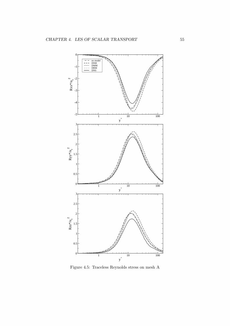
CHAPTER 4. LES OF SCALAR TRANSPORT 55
1 10 100
y+
-5
-4
-3
-2
-1
0
Rxx
*/u τ2
no modelDSMDMMDRMDNS
1 10 100
y+
0
0.5
1
1.5
2
2.5
3
Ryy
*/u τ2
1 10 100
y+
0
0.5
1
1.5
2
2.5
3
Rzz
*/u τ2
Figure 4.5: Traceless Reynolds stress on mesh A

CHAPTER 4. LES OF SCALAR TRANSPORT 56
1 10 100y
+
-1
-0.8
-0.6
-0.4
-0.2
0
h y
no modelDSMDMMDRMDNS
(a)
1 10 100y
+
-1
-0.8
-0.6
-0.4
-0.2
0
h y
DSMDRMDRM_DSMDNS
(b)
1 10 100y
+
-1
-0.8
-0.6
-0.4
-0.2
0
h y
DSMDMMDRMDRM_DSMDNS
(c)
Figure 4.6: Resolved and modelled temperature flux, hy = 〈v′φ′〉/uτTτ +〈γy〉/uτTτ on mesh A (a) and (b) and mesh B (c)

CHAPTER 4. LES OF SCALAR TRANSPORT 57
1 10 100
y+
-0.2
-0.15
-0.1
-0.05
0
< γ
y >/ (
uτT
τ)
DSMDMMDRM
Figure 4.7: Model subgrid heat flux hy for mesh A
the DRM better captures the velocity through the log-law region and the
buffer region than the DMM and DSM models, but it performs poorly in the
centre of the channel. In mesh A, the maximum cell dimension in the wall
normal direction is ∆y+ = 8.7. This should be sufficient for LES. The better
results of Gullbrand and Chow [80] suggest that the poor predictions of the
centre-line velocity may be a low Reynolds number effect. In the present
study with Reτ = 150, the log-law region is quite small (y+ ∼ 20−80). The
models in this study may not perform as well at low Reynolds numbers.
This may be due to the dynamic Smagorinsky term in the models. In the
less turbulent flow considered here, similarity between the test filtered level
( ˆG) and the G level, may not be as strong, possibly leading to an under
prediction of the model dissipation at the centre of the channel.
There is predictably a strong correlation between the predictions of the
scalar temperature profile and the mean velocity profile. The poor perfor-
mance of all the models at predicting the mean temperature profile, does
not necessarily mean that the models are inadequate for modelling γ. Both
the velocity field and the scalar SFS model determine the transport of φ.
The temperature profile appears to be more difficult to capture accurately
than the velocity profile. The sharp rise in temperature in the centre of the
channel which is seen in the DNS result, is not captured in any of the LES
simulations. This may again be a low Reynolds number effect which needs
to be tested.
CHAPTER 4. LES OF SCALAR TRANSPORT 58
4.8 Conclusions
Several large eddy simulation models have been examined within the frame-
work of explicit filtering and reconstruction outlined by Carati et al. [76].
The DMM and DRM models have been applied to the simulation of trans-
port of a passive scalar in a turbulent channel flow. Compared with the
DSM model and no-model, where no reconstruction is performed, the DMM
and DRM models perform quite well.
For the prediction of the turbulent stresses and the mean flow statistics,
all the models perform better than the ’no-model’ simulation. Both the
DMM and the DRM perform better than the DSM for most of the quantities
examined, particularly in the buffer region and through most of the log-law
region. The DRM model appears to offer some improvement over the DMM,
but overall the results are mixed. The DRM underpredicts the mean velocity
in the centre of the channel.
The results for the transport of a passive scalar are less successful. None
of the models predicted the correct mean temperature profile across the
channel. The DRM seems slightly better in the region close to the wall, but
underpredicts the temperature in the centre of the channel more severely
than the other models. The Nusselt numbers were similarly poorly pre-
dicted. The scalar flux from the wall was quite well predicted by the DRM
and DMM for y+ < 40. The no-model and DSM models performed more
poorly here. In the centre of the channel, the flux was over predicted by all
models.
Overall, it appears that the DRM and DMM are promising concepts, for
modelling both the scalar SGS model and the residual stress. For most of the
statistics examined, both models perform better than the DSM model. In
several of the statistics examined however, their performance was mixed, so
more work is needed before they can be trusted in more difficult simulations.
Further tests are needed at higher Reynolds number to confirm these results.
Having performed these calculations it is interesting to relate them back
to the simulation of a NDWCT. The computational cost or simulation time
of LES increases with the Reynolds number simulated. The scaling goes
like ∼ Re3. In this study, turbulent channel flow at Re = 4560 has been
examined. The Reynolds number for an entire NDWCT is ∼ 1.7 × 10⁷,
approximately 4×10³ times higher than that for the channel flow simulation.

CHAPTER 4. LES OF SCALAR TRANSPORT 59
Thus the computational time ∼ 5 × 10¹⁰ longer. With simulations in this
study taking approximately 40 hours in a single processor, this means a
similarly well resolved LES simulation of the entire cooling tower would
take in the order of 200 million years. Thus full tower modelling with well
resolved LES is completely unrealistic on modern computers. LES may be
able to be applied in some isolated small regions of the tower however, such
as an isolated small section of the fill.

Chapter 5
Two Dimensional
Axisymmetric NDWCT
Model
5.1 Introduction
In this chapter, a numerical model of a NDWCT is presented with its vali-
dation against manufacturers’ performance curves. In sections 5.2 to 5.10,
the detail of the heat and mass transfer calculations are presented and the
fill modelling approach validated. The overall model is validated in section
5.10 and in section 5.11 results are presented. More detailed analysis of the
results and a parametric study is contained in Chapter 6.
5.2 Model description
The numerical model has been built within FLUENT version 6.1 [40]. This
study only examines the flow in the tower under no-cross wind conditions, so
the mean flow should be two dimensional. Here a two-dimensional axisym-
metric model has been developed, as a full three dimensional model would
be too computationally expensive. The air/water flow in the tower has been
modelled using a two phase simulation. The gas phase (continuous phase)
has been modelled in Eulerian form as a mixture of air/water-vapour/water-
condensate. The second phase is the discrete water droplets in the spray
and rain zones. The droplets have been modelled using Lagrangian particle
60

CHAPTER 5. TWO DIMENSIONAL NDWCT MODEL 61
tracking in FLUENT, and this component is referred to as the discrete phase
model (DPM). The governing equations for incompressible steady air flow
can be written in general form as:
∇ · (ρuφ − Γφ∇φ) = Sφ, (5.1)
as given in Chapter 3. The flow properties of the Eulerian mixture compo-
nents and the DPM are given in Appendix B.
The very large range of scales in a NDWCT mean that it is impossible to
computationally represent all components of the tower numerically. Instead
the components that cannot appear directly in the model are represented
through source terms in Eqn. 5.1. The manner in which these source terms
are calculated and coupled with the continuous phase is detailed in the
following sections. The modelling of the drift eliminators, tower supports
and other features causing flow resistance is discussed in section 5.5. The
modelling of the air and water flow and the heat and mass transfer in the
fill is presented in section 5.7.
5.3 Domain and boundary conditions
The cooling tower geometry and specifications are based on a NDWCT
located at Mt. Piper Power Station (Delta Electricity), NSW, Australia;
designed by Hamon-Sobelco LTD, South Africa. This is a coal fired power
plant operating 2x660MW Units. Each unit is cooled by a NDWCT. The two
NDWCTs at this site have a history of underperforming, primarily due to
wind effects. The plant operators have been actively involved in a research
program to improve the performance of the NDWCTS [21, 36, 37]. The
towers at this site were chosen as the basis for this study as they are both
of a typical NDWCT design and the design and operating data were readily
available. The design parameters are given in Table 5.1 together with the
reference conditions used in this study. The performance curves from this
tower are used for the validation of the model.
The axisymmetric representation of the domain in this study is shown
in Fig. 5.1. In the reference tower, a 2.8m wide causeway runs through the
centre of the tower. This has been represented by a 1.4m wide blockage in
the axisymmetric model (see Fig. 5.1). The computational domain extends

CHAPTER 5. TWO DIMENSIONAL NDWCT MODEL 62
Table 5.1: Design parameters for the reference tower
Reference Conditions
Tower height 131mInlet height 8.577mFill depth 1.0mTower basin diameter 98mFill base diameter 93mWater flow rate 15,000kg/sWater inlet temperature 313KAmbient air temperature 295KAmbient air humidity 55%Ambient pressure 101kPaInlet turbulence intensity 5%
for 90m beyond the cooling tower inlet and 90m above the cooling tower
outlet as shown in Fig. 5.1. This ensures that the flow is fully developed
as it enters the cooling tower and that the flow leaving the tower is not
influenced by the outlet boundry condition. These values have been tested
(see section 5.8) and found to be sufficient.
At the wall boundaries noted in Fig. 5.1, no slip Dirichlet boundary
conditions are enforced for axial and radial momentum and zero gradient
Neumann boundary conditions used for energy and species. At the axis
boundary, the radial velocity is zero while temperature and species gradients
are zero. At the domain inlet and outlet, the inflow temperature and species
concentration are defined as given in Table 5.1. This can be written as
follows where φ is the scalar temperature or species and v is the axial velocity
component and u the radial component:
Wall Boundaries: dφdy = 0, dφ
dr = 0,u, v = 0
Outlet Boundary: dφdy = 0, du
dy = 0, dvdy = 0
Axis Boundary: dφdr = 0, du
dr = 0 u = 0
Inlet Boundary: φ = φin, dudr = 0, dv
dr = 0

CHAPTER 5. TWO DIMENSIONAL NDWCT MODEL 63
1 2 3456 InletHeight6?Ground WallInlet
OutletAxis ShellWall Rain ZoneSpray ZoneFill Zone �� �����������������������������
1
Figure 5.1: Computational domain (left) with heat and mass transfer regiondetail enlarged on right: (1) drift eliminators, (2) spray nozzles, (3) fill waterinlet (or fill air outlet), (4) fill water outlet (or fill air inlet), (5) basin, (6)causeway.
5.4 Solution procedure
An overview of the heat and mass transfer procedure and water flow repre-
sentation is as follows:
1. The water enters the tower through the spray nozzles. The water mass
flow rate and temperature are specified and droplet spray trajectories
are initiated at approximate nozzle locations across the tower (see
section 5.6.4).
2. The spray droplets pass through the spray zone (see Fig. 5.1) and
upon reaching the top surface of the fill, they are terminated and their
temperature is recorded and used as an input to the fill model.
3. In the fill an external procedure is used to determine the change in wa-
ter temperature and mass through the fill (section 5.7). This procedure
is implemented in subroutines, written in ’C’ programing language
and compiled directly into FLUENT through its USER-DEFINED-
FUNCTION (UDF) capabilities. The same procedure then calculates
the energy and mass source terms to couple the energy and mass trans-
fer with the continuous phase. Additionally, the procedure determines

CHAPTER 5. TWO DIMENSIONAL NDWCT MODEL 64
the momentum source terms representing the flow resistance the gas
phase experiences through the fill.
4. At the bottom of the fill the new water temperature and mass flow rate
are used to initiate the droplet flow in the rain zone (section 5.6.4).
5. The droplets pass through rain zone with heat, mass and momentum
coupled with the gas phase. On reaching the basin, the trajectories are
terminated and the temperature and mass of the droplets are recorded.
The above procedure together with the equations and numerical proce-
dures outlined in Chapter 3 are solved in FLUENT. The solution procedure
for the segregated solver with the subroutines for the fill and the discrete
phase model (DPM) is depicted in Fig. 5.2. The source terms in the fill
are updated every iteration. The DPM and the source terms coupling the
heat, mass and momentum transfer with the continuous phase are updated
every ten iterations. The solution proceeds until convergence. The solution
changes are relaxed according to Eqn. 5.2 with the relaxation factors given
in Table 5.2.
φnew = φold + αφ(φcalculated − φold) (5.2)
Table 5.2: Relaxation parameters
Flow variable (φ) Relaxation parameter (α)
Energy 0.5Mass 0.4
Radial momentum 0.3Axial momentum 0.3
DPM momentum source 0.3DPM energy source 0.3DPM mass source 0.3
5.5 Component losses
The pressure loss due to the tower shell supports, the spray piping network,
the fill supports and the drift eliminators are represented as a pressure loss

CHAPTER 5. TWO DIMENSIONAL NDWCT MODEL 65
1 Initialisation2 Begin loop3 Calculate the change in water temperature
and mass through the fill. Calculate the en-ergy, mass and momentum source terms forthe continuous phase
4 Calculate the condensation/evaporation en-ergy and mass source terms in the sprayzone and tower
5 Solve the axial momentum equation6 Solve the radial momentum equation7 Solve the pressure correction equation and
update velocity components8 Solve the energy equation9 Solve the species transport equations for
H2O mist/condensate, H2O vapour, O2,N2
10 Solve the turbulent kinetic energy equation(k − ǫ model)
11 Solve the turbulent kinetic energy dissipat-ion rate equation (k − ǫ model)
12 Update material physical properties13 Calculate droplet trajectories and ∆Tw,
∆Mw
14 Update source terms to couple the DPMwith the continuous phase
15 Check convergence(if not converged GO TO 3)
16 END
Figure 5.2: Segregated solver procedure

CHAPTER 5. TWO DIMENSIONAL NDWCT MODEL 66
@@@R
@@
@@R
Spray nozzles (Kwdn)
Drift eliminators and fill supports (Kde + Kfs)
Tower supports (Kcts) -
Figure 5.3: Model representation of pressure loss terms
implemented across an internal cell boundary in the model. The pressure
loss is calculated according to Eqn. 5.3:
∆P = kL1
2ρv2, (5.3)
where v is the normal component of velocity through the boundary face and
kL is the pressure loss coefficient. The loss coefficients for the tower shell
supports, the spray piping network, the fill supports and the drift eliminators
are Kcts = 0.5, Kwdn = 0.5, Kfs = 0.5 and Kde = 3.0 respectively as taken
from Kroger [1]. Additional discussion of tower losses is given in Chapter 7.
These losses have been implemented as close to the physical tower loca-
tions as possible in the model as shown in Fig. 5.3. The inlet losses due
to the tower shell supports are located at the inlet. Fill supports are thin
vertical struts in the rain zone supporting the weight of the fill pack. Physi-
cally these losses are distributed radially across the tower but implementing
this is complex with the only data available in the form of a single summed
loss coefficient. Instead the pressure loss due to the fill supports has been
implemented at the drift eliminator location.
5.6 Discrete phase model: rain and spray water
flow modelling
In the spray and rain regions, the water flows in droplet form. Most pre-
vious models [22, 23] assumed one-dimensional motion of the droplets or

CHAPTER 5. TWO DIMENSIONAL NDWCT MODEL 67
Droplet
Continuous Phase Cell
Droplet
Trajectory
Momentum, Heat
and Mass Transfer
@@
@R
Figure 5.4: Coupling of droplet flow with continuous phase model
represented them more coarsely through average transfer coefficients [5, 24].
Here the droplet flow has been modelled using Lagrangian particle tracking
with coupled heat and mass transfer between the droplets and the continu-
ous phase. The process is shown in Fig. 5.4. The material properties and
equation of state relations for this phase are given in Appendix B.
5.6.1 Droplet trajectory calculation
The droplet trajectory is calculated in the Lagrangian reference frame. The
droplet location is advanced in the x-direction by the step wise integration
of:dx
dt= ud. (5.4)
The instantaneous velocity in the x direction ud is found from a force
balance upon the droplet, equating the droplet inertia with drag and the
body force of gravity. Again for the x-direction this can be written as:
dud
dt= FD(u − ud) +
gx(ρd − ρ∞)
ρd, (5.5)
where FD(u − ud) is the drag force per unit mass and,
FD =18µ
ρdd2d
CDRed
24, (5.6)

CHAPTER 5. TWO DIMENSIONAL NDWCT MODEL 68
and the drag coefficient, CD, is calculated using Eqn. 5.7,
CD = a1 +a2
Red+
a3
Red2 , (5.7)
where the coefficients a1, a2, a3 are taken from Morsi and Alexander [100].
The droplet Reynolds number, Red, is given by,
Red ≡ ρdd |ud − u∞|µ
. (5.8)
The droplet trajectory is determined advancing the droplet location over
small discrete time intervals with the step-wise integration in each coordinate
direction of Eqn. 5.4 in time and Eqn. 5.5 in space. These equations are
discretised using a trapezoidal scheme. The new particle velocity at time
n + 1 is found using:
un+1d =
und (1 − 1
2∆tFD) + ∆tFD
(un∞
+ 12∆tun
d · ∇un∞
)+ ∆t gx(ρd−ρ∞)
ρd
1 + 12∆tFD
.
(5.9)
The new droplet location, xn+1d , can then be found using:
xn+1d = xn
d +1
2∆t(un
d + un+1d
). (5.10)
The time step for the integration ∆t has been set by specifying λ, the
number of time steps to be computed as a droplet crosses a cell. FLUENT
estimates ∆t∗, the droplet residence time in a cell and the time step for
integration is computed using:
∆t =∆t∗
λ. (5.11)
In this study λ has been set to 5.
5.6.2 Heat and mass transfer
This section closely follows the combined heat and mass transfer discussion
in Chapter 2. In FLUENT, the temperature change of the evaporating water
droplet is described in the Lagrangian reference frame as given in Eqn. 5.12:
mdCddTd
dt= hAd(T∞ − Td) +
dmd
dtifgwo. (5.12)
CHAPTER 5. TWO DIMENSIONAL NDWCT MODEL 69
The term hAd(T∞ − Td) represents the sensible heat transfer between the
gas phase and the droplet and dmd
dt ifgwo the latent heat transfer from evap-
oration. ifgwo is the latent heat of water at 0oC. T∞ is the temperature in
Kelvin of the gas phase in the cell that the droplet is currently in, Td is the
droplet temperature, Ad is the droplet surface area, h is the heat transfer
coefficient, ifgwo is the latent heat of vaporisation, Cp is the specific heat of
water evaluated at the droplet temperature and md is the droplet mass in
kg.
The mass transfer from the droplet due to evaporation is described by:
N = kc(Cs − C∞), (5.13)
where N is the molar flux of vapour species with units (kgmol/m2s), kc is the
mass transfer coefficient m/s and C∞ is the concentration of water vapour
in the bulk gas phase (kgmol/m3). Cs is the molar concentration of water
vapour at the droplet surface, calculated assuming the vapour pressure at
the droplet surface is equal to the saturated vapour pressure Psat, calculated
at the droplet temperature. Cs and C∞ are given by Eqn. 5.14 and Eqn.
5.15 respectively:
Cs =Psat,Td
RTd, (5.14)
C∞ = XPop
RT∞
, (5.15)
where R is the universal gas constant, Pop is the operating pressure and X
is the mole mass fraction of the evaporating species. The new droplet mass
is updated following Eqn. 5.16:
md(t + ∆t) = md(t) − NAdMw∆t, (5.16)
where Mw is the molecular weight of water in kg/kmol. The heat and mass
transfer coefficients used in these equations are derived from the empirical
correlations given in Eqn. 5.17 and Eqn. 5.18 below. These correlations,
taken from [1, 40], are valid for 2 ≤ Red ≤ 800. In this study the droplet
Reynolds number in the spray zone is Red ≈ 1000 − 1200, just above the
upper limit of the correlation. In the rain zone 15 . Red . 1400. While the
upper range in the rain zone is somewhat above the limits of the empirical
correlation, the mean Red based on the average conditions in the rain zone

CHAPTER 5. TWO DIMENSIONAL NDWCT MODEL 70
and sauter mean diameter of the droplet distribution, is Red ≈ 430 which is
in the middle of the valid range for the correlations, so is reasonable for use
in this study.
Sh =hDdd
Dm= 2.0 + 0.6Re
1/2d Sc1/3 (5.17)
Nu =hdd
k∞= 2.0 + 0.6Re
1/2d Pr1/3 (5.18)
If the droplet temperature falls below the dew point temperature of the
gas phase then condensation would naturally occur. However under these
conditions, the droplet is treated as inert in FLUENT and no mass transfer
occurs. Condensation of water vapour and evaporation of mist/condensate
in the gas phase are discussed in the next section.
5.6.3 Discrete phase-continuous phase coupling
The heat, mass and momentum transfer from the discrete phase is coupled
with the continuous phase through source terms as given below and depicted
in Fig. 5.4. The momentum source (Smom) or sink in the continuous phase
due to the change in droplet momentum across a cell control volume is given
in Eqn. 5.19.
Smom =
(18µCDRed
ρdd2d24
(ud − u∞)
)md∆t (5.19)
The evaporation from the droplets is coupled with the continuous phase
through the vapour transport equation and the continuity equation. The
source term is given by Eqn. 5.20,
Sv = ∆md, (5.20)
where ∆md is the change in droplet mass across a cell control volume. Sim-
ilarly the energy source term for the gas phase is given by Eqn. 5.21,
Sq = mdCp∆Td + ∆md
(− ifgwo +
Td∫
Tref
CpdT), (5.21)
where ∆Tp and ∆mp are the changes in temperature and mass of the droplet
across a cell and Tref is 273.15 Kelvin.
In this model, there is the potential for the gas phase to become super-
saturated. In cells where this occurs a separate algorithm is run iteratively

CHAPTER 5. TWO DIMENSIONAL NDWCT MODEL 71
if (RH >1 ) or (if RH <1 and φmist >0) then:Sv = Sv + C(ω′′ − ω)Smist = −Sv
Sq = ifgwoSmist
Figure 5.5: Condensation routine procedure
to ensure that any additional vapour in the gas phase in excess of the sat-
uration level is transfered to the condensate component of the continuous
phase with the latent heat source put back into the vapour mixture. Simi-
larly if the gas phase becomes unsaturated then the condensate evaporates
with the latent heat absorbed from the continuous phase. The procedure is
outlined in Fig. 5.5, where C = 0.6, Sv is the vapour source, Smist is the
condensate/mist source and Sq is the energy source term.
5.6.4 Spray and rain zone modelling
Spray zone
Large cooling towers use spray nozzles that operate at relatively low pres-
sure, between 5000-15000N/m2 [1] (∼ 0.5m − 1.5m static pressure head).
The reference tower in this study has spray nozzle diameters between 30mm
and 33mm with approximately 0.5m of water static pressure head available.
The water flow rate is 2.2kg/s per nozzle. Very little work on low pressure
spray nozzles of this type has appeared in literature.
Lowe and Christie [7] give the transfer characteristics for a fine spray
system in terms of spray pressure, height through which the droplets fall
and the air flow rate. The spray head ranged from ∼ 1.2 − 3.6m and the
Sauter mean diameter ranged between 0.90−1.28mm. The data shows that
the mean diameter increases significantly with the distance the droplet falls
(depth of spray zone). The author suggests that after ∼ 0.6m the spray may
agglomerate and lose any of the advantage of high pressure spraying.
Bellagamba et al. [101] conducted an experimental study of four spray
nozzles used for cooling tower applications. The geometry and pressure
head of the nozzle ’C’ in that study are very similar to the nozzle type in
the reference NDWCT in the current study. The mass flow rate is a little

CHAPTER 5. TWO DIMENSIONAL NDWCT MODEL 72
Figure 5.6: Spray droplet trajectories at centre of tower coloured by tem-perature
Spray Nozzles
Fill Top
Fill Bottom
lower at 1.5kg/s however and the diameter of this nozzle is 25mm. These
characteristics are thought to be close enough so the characteristics of this
nozzle have been employed here.
In this study, the water flow from each nozzle has been represented by
20 trajectories. A uniform droplet size of 2.8mm has been used with an
initial axial velocity of 0m/s. At each nozzle the initial radial velocity of
the droplets varies linearly between −6.3m/s to +6.3m/s. The injection
points have been spaced at 0.9m intervals along the tower radius consistent
with nozzle locations in the reference tower.
A visualisation of the droplet trajectories in the spray zone from a sim-
ulation (under reference conditions in Table 5.1) are given in Fig. 5.6. The
two dimensional representation of the spray ignores variation in spray in the
circumferential direction.
Rain zone
The characteristics of the droplet distribution in the rain zone depends sig-
nificantly on the fill type with splash type fills producing drops between
3mm − 4mm and film and trickle packs producing larger droplets between
5mm − 6mm [1]. Kroger [1] provides a sample distribution from a splash
pack type fill with a Sauter mean diameter of 3.26mm. The Sauter mean
diameter, is the diameter of a sphere which has the same volume to surface
area ratio as the entire distribution of spheres, which it is derived from. It
is useful for heat and mass transfer problems where the surface contact area

CHAPTER 5. TWO DIMENSIONAL NDWCT MODEL 73
is of interest. It is defined as,
dsm =∑
i
ndid3di/∑
i
ndid2di, (5.22)
where ndi is the number of droplets of diameter ddi in a sample. This
distribution was employed in this work after personal communication with
the author 1. The smallest droplet size in the distribution given by Kroger
[1], is actually 0.25mm. In the present study, the mass fraction at this
droplet size was given to a droplet diameter of 0.5mm to prevent problems
of droplet entrainment in the flow. This has a negligible effect on the flow
and the sauter mean diameter remains the same. In this study, the rain
zone has been represented by 6,810 droplet trajectories across 454 injection
locations. At each injection point the droplet distribution is represented with
15 trajectories as given below in Table 5.3. An injection point is initiated
in every cell face on the bottom of the fill.
Table 5.3: Droplet distribution in the rain zoneDiam (mm) 0.50 0.75 1.25 1.75 2.25
Mass Fraction 0.000147 0.0189 0.0703 0.0912 0.0572
Diam (mm) 2.75 3.25 3.75 4.25 4.75Mass Fraction 0.0454 0.0374 0.0460 0.0502 0.0935
Diam (mm) 5.25 5.75 6.25 7.25 8.25Mass Fraction 0.0947 0.0829 0.107 0.0831 0.122
5.7 Fill representation
5.7.1 Introduction
It would be computationally too expensive to model complex water and air
flow through the fill explicitly so the effect of the fill on the continuous phase
is represented using volumetric source terms based on empirical pressure loss
coefficients and transfer coefficients. The fill is physically represented in the
model as a region where the gas phase flow is restricted to flow in the vertical
direction only.
1Kroger, D. (personal communication, 2004) University of Stellenbosch, South Africa

CHAPTER 5. TWO DIMENSIONAL NDWCT MODEL 74
Ta,m, ωm
Ta,3, ω3
Ta,2, ω2
Ta,1, ω1
Tw,n+1,mw,n+1
Tw,n,mw,n
Tw,3,mw,3
Tw,2,mw,2
Tw,1,mw,1
Tw,0,mw,0
Overlaid 1D gridwater flow representation
Layer m
Layer 3
Layer 2
Layer 1
Continuous Phase
Figure 5.7: Schematic of fill representation
Schematically, the external procedure for calculating the source terms
can be depicted as in Fig. 5.7. The fill region is subdivided into a number
of vertical columns each one mapped onto a separate one dimensional grid
where the water flow variables are stored. The water flow is then represented
solely by two variables at each point on this grid, its temperature and mass
flow rate. Across each layer in these columns, or between points on the one
dimensional grid, the change in water temperature and mass are computed
and this result is then coupled with the continuous phase through source
terms in each layer of the vertical columns.
The water flow through the tower fill is represented by 78 of these
columns with each one discretised into 10 layers or nodes. The width of
the columns range between 1.0m and 0.1m with the narrow columns packed
into regions of high air velocity gradient, near the tower centre and outer
regions (see Table 5.6).
5.7.2 Momentum sink
The pressure loss through fill is modelled using volumetric source terms in
the momentum equation. This momentum sink is given in Eqn. 5.23:
Sv = −KfiρV 2
2. (5.23)
In this way, the fill resistance to air flow is measured by its loss coefficient
in a similar manner to the component losses in section 5.5. Like the transfer

CHAPTER 5. TWO DIMENSIONAL NDWCT MODEL 75
characteristics, they are given as an empirical function of the dependent
variables, usually, the fill depth Lfi, the air mass flux Ga and the water
mass flux Gw.
Several forms of the empirical correlations have appeared in the lit-
erature. Lowe and Christie [7] presented their widely cited data using
Eqn. 5.24, where Kfi/Lfi gives the fill loss coefficient per unit fill depth.
Goshayshi and Missenden [2] correlated their data using Eqn. 5.25. Another
common form of the coefficient is given in Eqn. 5.26 [1]. The constants c1−c4
that appear in these correlations are found from experiment and are specific
to a particular model of fill. Kroger [1] gives a comprehensive summary
of the correlations available in literature with coefficients for a range of fill
types.
Kfi
Lfi= c1
Gw
Ga+ c2 (5.24)
Kfi
Lfi= c1G
c2w Gc3
a (5.25)
Kfi
Lfi= c1G
c2w Gc3
a Lc4fi (5.26)
Kloppers and Kroger [3] investigated the functional dependence of the
loss coefficient for trickle grid fills. They found that the coefficient is a
function of fill depth but not of air or water temperature. The authors
proposed a new form of the empirical equation as given in Eqn. 5.27:
Kfi
Lfi= c1G
c2w Gc3
a + c4Gc5w Gc3
a . (5.27)
The authors also developed a more general correlation as a function of fill
depth as given by Eqn. 5.28,
Kfi
Lfi= (c1G
c2w Gc3
a + c4Gc5w Gc6
a )Lc7fi. (5.28)
In this study, all the loss coefficients for the fill have been taken from Klop-
pers and Kroger’s work [3, 102] and are given in Eqns. 5.29-5.31:

CHAPTER 5. TWO DIMENSIONAL NDWCT MODEL 76
Kfi,0.6m
Lfi= (0.003132G4.755218
w G−3.631669a
+17.238242G0.349702w G−0.030826
a ) (5.29)
Kfi,0.9m
Lfi= (1.561219G1.276792
w G−3.931459a
+16.173258G0.287875w G0.011599
a ) (5.30)
Kfi,1.2m
Lfi= (3.859490G0.782298
w G−2.119420a
+15.295976G0.215311w G0.080546
a ) (5.31)
These correlations are developed at discrete fill depths of 0.6m, 0.9m and
1.2m. The relations were correlated with experimental data over the range
2.7kg/s/m2 < Gw < 6.1kg/s/m2 and 1.2kg/s/m2 < Ga < 4.2kg/s/m2
[3, 102]. In this study water mass flux’s of 2.2kg/s/m2 − 4.4kg/s/m2
and air mass flux’s of ∼ 1.4kg/s/m2 − 2.4kg/s/m2 are considered. At
the reference conditions Gw = 2.21kg/s/m2 and the average air mass flux
Ga ∼ 1.8kg/s/m2. The air mass flux is well within the experimental range
but the water mass flux is slightly below the lower bound, meaning the cor-
relation may not be accurate. The difference is small however and has been
deemed acceptable in this work.
In this study a range of fill depths have been modelled. The correlations
in Eqns. 5.29-5.31 were used for the cases where the fill depth corresponded
to one of the three depths given above. Elsewhere, and for the reference
tower with a fill depth of 1.0m, a combination of the original correlations
have been used by applying an interpolation function as given in Eqn. 5.32
and Eqn. 5.33,
KP,fi,Lfi= KP,fi,0.9mf + KP,fi,1.2m(1 − f), (5.32)

CHAPTER 5. TWO DIMENSIONAL NDWCT MODEL 77
where the smoothing factor f =(1.2−Lfi)(1.2−0.9) for 0.9 < Lfi < 1.2 and
KP,fi,Lfi= KP,fi,0.6mf + KP,fi,0.9m(1 − f), (5.33)
where the smoothing factor f =(0.9−Lfi)(0.9−0.6) for 0.6 < Lfi < 0.9. This approach
was found to give smoother fit to the data in the range of air and water flow
rates considered here than a single general correlation developed for all fill
depths and water flow rates using Eqn. 5.28.
The implementation of this routine has been tested against the experi-
mental data in Kloppers thesis [3] found to return the correct pressure drop.
5.7.3 Heat and mass transfer in the fill
The heat and mass transfer characteristics of the fill are derived from em-
pirical transfer coefficients in the form of the Poppe Merkel number. The
correlations for the fill type in the reference tower were not available so other
data given in Kloppers’ thesis [3] for a similar film fill, have been used.
As the heat and mass transfer characteristics of the fill are defined
through the Merkel number for the Poppe method, any method implemented
in this numerical model must be equivalent to the Poppe method. Because
the Poppe method does not introduce any additional assumptions into the
model, other than the one dimensional ones discussed in section 2.2 and sec-
tion 5.7.1, this becomes very easy. The heat and mass transfer is specified
through Eqns. 2.1-2.4.
The empirical transfer coefficients conveniently yield the heat and mass
transfer coefficients together with the contact area between the phases. With
hmA known, the product of the heat transfer coefficient and contact surface
area, hA, can be found by re-arranging the Lewis factor relationship,
Lef =h
hmCpm, (5.34)
to give,
hA = LefhmACpm. (5.35)
Following Poppe’s approach [10], the Lewis factor can be found from Bosj-

CHAPTER 5. TWO DIMENSIONAL NDWCT MODEL 78
nakovics formula [1],
Lef = 0.8652/3 ·
(ω′′
Tw+0.622ω+0.622 − 1
)
ln
(ω′′
Tw+0.622
ω+0.622
) . (5.36)
Bosjnakovics formula under saturation conditions is modified, as shown in
Appendix A. The transfer coefficient used here is written in terms of the fill
air and water inlet flow rates, as shown in Eqns. 5.37-5.39 (taken from [3]):
MeP,0.6m
Lfi=
hmA
mwLfi
= 1.497125G0.276216w G0.665735
a
− 0.589942G0.634757w G0.622408
a (5.37)
MeP,0.9m
Lfi=
hmA
mwLfi
= 1.526182G0.078237w G0.695680
a
− 0.556982G0.419584w G0.675151
a (5.38)
MeP,1.2m
Lfi=
hmA
mwLfi
= 1.380517G0.112753w G0.698206
a
− 0.517075G0.461071w G0.681271
a (5.39)
The above relations give the Poppe Merkel number per unit fill depth and
as for the loss coefficients, the correlations are developed at discrete fill
depths of 0.6m, 0.9m and 1.2m, with experimental data over the range
2.7kg/s/m2 < Gw < 6.1kg/s/m2 and 1.2kg/s/m2 < Ga < 4.2kg/s/m2 [3,
61]. Again, operating point for the reference cooling tower modelled in this
study is at a mass flux of Gw = 2.21kg/s/m2 slightly below this range of
experimental data. The difference is small however and has been deemed
acceptable in this work.

CHAPTER 5. TWO DIMENSIONAL NDWCT MODEL 79
The data in Kloppers’ thesis [3] has also been used here to develop a
general correlation for the Poppe Merkel number as a function of fill depth,
MeP,gen
Lfi=
hmA
mwLfi= 1.118G−0.389
w G0.735a L−0.280
fi . (5.40)
The regression analysis used was similar to that used by Kloppers [3] to fit
the same data to a general correlation using the Merkel model (Eqn. 7.5).
The regression analysis used here successfully reproduced Kloppers other
correlations. The correlation R2 value for this fitted equation is 0.9873.
This equation has been used for the cases where the fill depth simulated did
not match one of the three given above.
5.7.4 Coupling procedure
The calculations across each layer take place between the averaged continu-
ous phase flow variables and the water flow variables on the one dimensional
grid (Fig. 5.7). The source terms calculated are identical for all the cells
across the layer.
The water evaporated, mmevap, across fluid layer m is determined using
Eqn. 5.41, where ω is the average specific humidity in the fluid zone and
∆Lfi is the height of the current layer. If the air is super-saturated then
Eqn. 5.42 is used:
mmevap = hmA
(∆Lfi
Lfi
)(ωm
sat,Tw − ωm), (5.41)
mmevap = hmA
(∆Lfi
Lfi
)(ωm
sat,Tw − ωmsat,Ta). (5.42)
The equivalent relation for Eqn. 5.41 in Chapter 2 is Eqn. 2.1. Eqn. 5.42 is
equivalent to Eqn. A.30 in Appendix A. The downstream water mass flow
rate is found using Eqn. 5.43:
mnw = mn+1
w − mmevap. (5.43)
The latent and sensible heat transfer is evaluated using Eqns. 5.44 and 5.45
CHAPTER 5. TWO DIMENSIONAL NDWCT MODEL 80
respectively (c.f. Eqn. 2.4 and 2.5 in Chapter 2):
qmlatent = mm
evapifgwo, (5.44)
qmsensible = hA((T n+1
w + T nw)/2 − Tm
a ), (5.45)
where Tma is the average temperature of the continuous phase in the layer.
The water temperature at the inter-facial layer n is determined using:
T nw = T n+1
w − (qmsensible + qm
latent)
Cpwmn+1w
. (5.46)
When the flow becomes super-saturated, water vapour condenses as mist
(mmcond) and the latent heat of vaporisation is released into the mixture. It
has been assumed for this investigation, as in the Poppe model [3, 10],
that vapour condenses as mist when the vapour pressure rises above the
saturation vapour pressure.
The mass source Ms and enthalpy source Qs per unit volume are given
by Eqns. 5.47 and 5.48:
Mms =
mmevap
∆Lfi, (5.47)
Qms = (mn+1
w Cpw∆Tmw + mm
evap(Cpv(Tn+1w + T n
w)/2
−298.15) − ifgwo))/∆Lfi + mmcondifgwo. (5.48)
5.7.5 Model validation
In order to validate this approach, it has been compared against the pre-
dictions of the Poppe model described in Chapter 2. The Poppe equations
(see Appendix A) were numerically integrated using the non-stiff ODE45
Runge-Kutta numerical integration procedure in Matlab [103], a commer-
cial mathematical programing software. The ODE45 procedure uses an au-
tomatic step size selection algorithm which in this case reaches completion
after approximately 70 discrete steps. The comparison has been performed
under the conditions given in Table 5.4. The air and water fluid properties
are based on those in Kroger [1] and are given in Appendix 1.
The Poppe model solution and the CFD routine with 40 nodes/layers
through the fill are compared with and without the effects of condensation
included. For both methods, ignoring condensation here simply means ig-

CHAPTER 5. TWO DIMENSIONAL NDWCT MODEL 81
Table 5.4: Test parameters
ωi 0.012kg/kgTw,i 40oCTa,i 20oCGa 1.5kg/s/m2
Gw,i 2.4kg/s/m2
MEp 1.0δME 5 × 10⁻⁵
δω 1 × 10⁻⁴
noring the switch to use the alternate equations when the relative humidity
rises above 100%. This has been done to demonstrate the importance of
condensation to the problem.
The comparison of the two models is given in Figs. 5.8-5.9 at an air
mass flux of Ga = 1.5kg/s/m2 and Ga = 2.5kg/s/m2 respectively. The
water temperature, air temperature and relative humidity have been plot-
ted against Poppe Merkel number as the numerical integration proceeds,
showing how the solutions diverge when saturation in not included.
The importance of condensation in the calculation is clear. When con-
densation is ignored, the relative humidity is allowed to rise above 100% and
the two solutions diverge. If latent heat is released, the energy and mass bal-
ance changes significantly, with the air temperature rising when saturation
is included. The water outlet temperature does not register a noticeable
change however. In a full NDWCT calculation, the inaccurate prediction
of the air temperature leaving the fill could lead to an under-estimate the
tower draft and therefore the air-flow rate. This could then lead to a more
significant change in water outlet temperature. The curves for the Poppe
model and the CFD model match well, both with and without condensa-
tion indicating that the physics of the problem is well captured in the CFD
model and that the models are essentially equivalent.
Table 5.5 gives a comparison of the predicted water outlet temperature
from the Poppe method and the CFD numerical procedure under the con-
ditions in Table 5.4. With greater than five nodes through the depth, there
is very little improvement in model prediction. In this work ten nodes or
layers were used.

CHAPTER 5. TWO DIMENSIONAL NDWCT MODEL 82
0 0.1 0.2 0.3 0.4 0.5 0.6 0.7 0.8 0.9 120
22
24
26
28
30
32
34
Air
Tem
pera
ture
(o C)
Poppe Merkel No.
CFD (sat)CFD (unsat)Poppe (sat)Poppe (unsat)
(a)
0 0.1 0.2 0.3 0.4 0.5 0.6 0.7 0.8 0.9 128
30
32
34
36
38
40
Wat
er T
empe
ratu
re (o C
)
Poppe Merkel No.
CFD (sat)CFD (unsat)Poppe (sat)Poppe (unsat)
(b)
0 0.1 0.2 0.3 0.4 0.5 0.6 0.7 0.8 0.9 10.8
0.85
0.9
0.95
1
1.05
1.1
1.15
Rel
ativ
e H
umid
ity
Poppe Merkel No.
CFD (sat)CFD (unsat)Poppe (sat)Poppe (unsat)
(c)
Figure 5.8: Comparison of heat and mass transfer characteristics of Poppemethod and equivalent CFD implementation through the depth of the fillwith Ga = 1.5kg/s/m2

CHAPTER 5. TWO DIMENSIONAL NDWCT MODEL 83
0 0.1 0.2 0.3 0.4 0.5 0.6 0.7 0.8 0.9 120
21
22
23
24
25
26
27
28
29
30
Air
Tem
pera
ture
(o C)
Poppe Merkel No.
CFD (sat)CFD (unsat)Poppe (sat)Poppe (unsat)
(a)
0 0.1 0.2 0.3 0.4 0.5 0.6 0.7 0.8 0.9 128
30
32
34
36
38
40
Wat
er T
empe
ratu
re (o C
)
Poppe Merkel No.
CFD (sat)CFD (unsat)Poppe (sat)Poppe (unsat)
(b)
0 0.1 0.2 0.3 0.4 0.5 0.6 0.7 0.8 0.9 10.8
0.85
0.9
0.95
1
1.05
1.1
1.15
Rel
ativ
e H
umid
ity
Poppe Merkel No.
CFD (sat)CFD (unsat)Poppe (sat)Poppe (unsat)
(c)
Figure 5.9: Comparison of heat and mass transfer characteristics of Poppemethod and equivalent CFD implementation through the depth of the fillwith Ga = 2.5kg/s/m2

CHAPTER 5. TWO DIMENSIONAL NDWCT MODEL 84
Table 5.5: Comparison of water outlet temperature predictions from Poppemethod and a CFD test section
No. of Nodes Trange (K) Mesh size Difference (K)
CFD 5 nodes 9.89 0.2 0.69CFD 10 nodes 10.54 0.1 0.036CFD 20 nodes 10.57 0.05 0.012CFD 40 nodes 10.57 0.025 0.0063
Poppe (Runge-Kutta) 10.58 N/A 0
5.8 Domain and mesh independence studies
A range of domain sizes, meshing schemes and grid sizes were used to test
model independence from these parameters. The fill is represented using a
regular structured grid with cell dimensions of 0.1m square. The fill itself is
10 cells deep by 454 cells wide. This was kept constant for all the following
mesh studies. The width of the fill columns was arranged as given in Table
5.6.
Table 5.6: Fill model column width
Column numbers(from centre)
1-7 8-17 18-48 50-58 60-68 70-78
Column width 0.20m 0.50m 1.00m 0.50m 0.20m 0.10m
Table 5.7: Grid independence
Mesh ElementsNo. Description
Total Elements Heat Transfer ZonesTrange(K)
1 Structured 207,250 84,230 13.792 Unstructured 380,588 257,568 13.763 Unstructured 548,958 257,568 13.76
Three meshes were employed to determine grid independence. The re-
sults in Table 5.7 show that doubling the number of mesh points from mesh
(1) to mesh (3) results in a change in water outlet temperature of less than
0.03K (∼ 0.2% of tower range). The results suggest that the number of
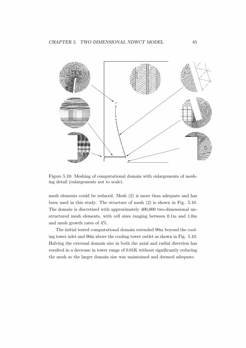
CHAPTER 5. TWO DIMENSIONAL NDWCT MODEL 85
ZZ
ZZ
ZZ~
SS
SS
SS
SSwPPPq
��
��
��
��
��
��
��
��=
��
��
��
��
��
��
��+
�������������9
Figure 5.10: Meshing of computational domain with enlargements of mesh-ing detail (enlargements not to scale).
mesh elements could be reduced. Mesh (2) is more than adequate and has
been used in this study. The structure of mesh (2) is shown in Fig. 5.10.
The domain is discretised with approximately 400,000 two-dimensional un-
structured mesh elements, with cell sizes ranging between 0.1m and 1.0m
and mesh growth rates of 4%.
The initial tested computational domain extended 90m beyond the cool-
ing tower inlet and 90m above the cooling tower outlet as shown in Fig. 5.10.
Halving the external domain size in both the axial and radial direction has
resulted in a decrease in tower range of 0.01K without significantly reducing
the mesh so the larger domain size was maintained and deemed adequate.

CHAPTER 5. TWO DIMENSIONAL NDWCT MODEL 86
5.9 Model sensitivity
Sensitivity to loss coefficient
A range of parameters for the drift eliminator loss coefficient and other
coefficients exist in literature. The loss coefficient for the tower supports
(see Fig. 5.3) was increased from 0.5 to 1.5 to test model sensitivity. The
resulting change in water temperature and flow field was negligible.
Sensitivity to initial radial velocity and diameter of spray droplets
The axial velocity of the droplets in the spray zone has been maintained at
0.0m/s in line with experimental results in Bellagamba [101]. The maximum
initial radial velocity and diameter of the droplets in the spray zone have
been examined. Here the maximum radial velocity has been doubled from
±6.3m/s to ±12.6m/s and the droplet diameter doubled from 2.8mm to
5.6mm. The results in Table 5.8 show that the overall model is insensitive
to radial velocity but somewhat sensitive to a very large increase in droplet
diameter.
Table 5.8: Sensitivity of model to spray parameters
Droplet initial Maximum radialdiameter (mm) velocity (m/s)
Tower range (K)
2.8 12.6 13.792.8 6.3 13.765.6 12.6 13.555.6 6.3 13.46
Sensitivity to initial axial velocity of rain droplets
The initial velocity of the droplets entering the rain zone has been assumed
to be 0.0m/s in both the radial and axial directions. A range of initial axial
velocities were tested to ensure model independence from this parameter. An
increase in initial axial velocity from 0m/s to 0.5m/s resulted in a decrease
in tower range of 0.046K ( ∼ 0.3%) and an increase from 0m/s to 1m/s
resulted in a decrease of 0.07K (∼ 0.5%), indicating that the model is not
sensitive to this parameter. This is not surprising as de Villers and Kroger

CHAPTER 5. TWO DIMENSIONAL NDWCT MODEL 87
0
2
4
6
8
10
12
14
16
18
20
284 286 288 290 292 294 296 298 300
Tow
er R
ange
(T
w,in
- T
w,o
ut)
(K)
Ambient drybulb temperature (K)
RH = 40% CFDRH = 40% manufacturers data
RH = 61.4% CFDRH = 61.4% manufacturers data
Figure 5.11: Model validation
[104] reported that the initial axial velocity of the droplets in the rain zone
makes very little difference if they are less than 10% of the terminal velocity.
In Chapter 7, a more detailed discussion of the rain zone parameters is given.
5.10 Validation
Final model validation was attempted by plotting the results from the nu-
merical model against the performance curves for the Mt. Piper cooling
towers introduced in section 5.3. Once again, the fill transfer coefficients
and loss coefficients were not available for these towers, so correlations for a
geometrically similar fill type were used. Differences in the fill performance
characteristics may be responsible for some of the error in this validation.
The performance curves give the tower range (Trange = Tw,i − Tw,o) for a
range of atmospheric temperatures and relative humidities. The comparison
given in Fig. 5.11 shows close agreement at low ambient temperatures with
the difference rising to 0.7K at an air temperature of 300K. The manufac-
turers’ supplied data is conservative at all temperatures.
The limited validation presented does not allow for rigorous validation
of the air flow field or relative accuracy of the heat and mass transfer in
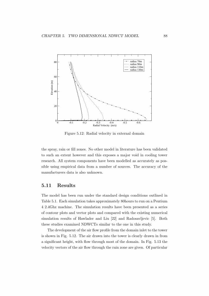
CHAPTER 5. TWO DIMENSIONAL NDWCT MODEL 88
-0.6-0.5-0.4-0.3-0.2-0.10Radial Velocity (m/s)
0
20
40
60
80
Ele
vatio
n (m
)
radius 70mradius 90mradius 110mradius 130m
Figure 5.12: Radial velocity in external domain
the spray, rain or fill zones. No other model in literature has been validated
to such an extent however and this exposes a major void in cooling tower
research. All system components have been modelled as accurately as pos-
sible using empirical data from a number of sources. The accuracy of the
manufacturers data is also unknown.
5.11 Results
The model has been run under the standard design conditions outlined in
Table 5.1. Each simulation takes approximately 80hours to run on a Pentium
4 2.4Ghz machine. The simulation results have been presented as a series
of contour plots and vector plots and compared with the existing numerical
simulation results of Hawlader and Liu [22] and Radosavljevic [5]. Both
these studies examined NDWCTs similar to the one in this study.
The development of the air flow profile from the domain inlet to the tower
is shown in Fig. 5.12. The air drawn into the tower is clearly drawn in from
a significant height, with flow through most of the domain. In Fig. 5.13 the
velocity vectors of the air flow through the rain zone are given. Of particular

CHAPTER 5. TWO DIMENSIONAL NDWCT MODEL 89
1.15e+01
1.01e-04
5.77e-01
1.15e+00
1.73e+00
2.31e+00
2.89e+00
3.46e+00
4.04e+00
4.62e+00
5.20e+00
5.77e+00
6.35e+00
6.93e+00
7.51e+00
8.08e+00
8.66e+00
9.24e+00
9.82e+00
1.04e+01
1.10e+01
1.15e+01
1.01e-04
5.77e-01
1.15e+00
1.73e+00
2.31e+00
2.89e+00
3.46e+00
4.04e+00
4.62e+00
5.20e+00
5.77e+00
6.35e+00
6.93e+00
7.51e+00
8.08e+00
8.66e+00
9.24e+00
9.82e+00
1.04e+01
1.10e+01
(a) (b)
Figure 5.13: Vector plots of air flow in the tower inlet (a) and at approxi-mately half the radius from centre (b)
interest, is determining if there is any re-circulation zone under the fill near
the inlet. It has been noted in literature that such conditions can exist [1, 22],
leading to an ineffective area of the fill and reduced performance. In Fig.
5.13 (a) the inlet region is given, showing the air flow entering the tower.
There is no re-circulation zone present under the fill or in the fill itself. In
Fig. 5.13 (b), the air flow in the centre of the tower is given as it enters the
fill, being drawn up at ∼ 45 degrees. The air flow through the rain region
is presented in Fig. 5.14 as path/stream lines, again showing the absence of
any recirculation zone in the tower. In none of the simulations performed
in this study, over a wide range of design parameters, was a re-circulation
zone observed.
In Fig. 5.15 the contours of pressure, air temperature, relative humidity
and velocity magnitude are given for the rain zone, spray zone and fill and
then again for the entire tower in Fig. 5.16.
The radial increase in air temperature and humidity is clear in Fig. 5.15
(a) and (b). The air in the rain zone becomes saturated close to the centre of
the tower. The distribution of droplet sizes in the rain zone leads to an inter-
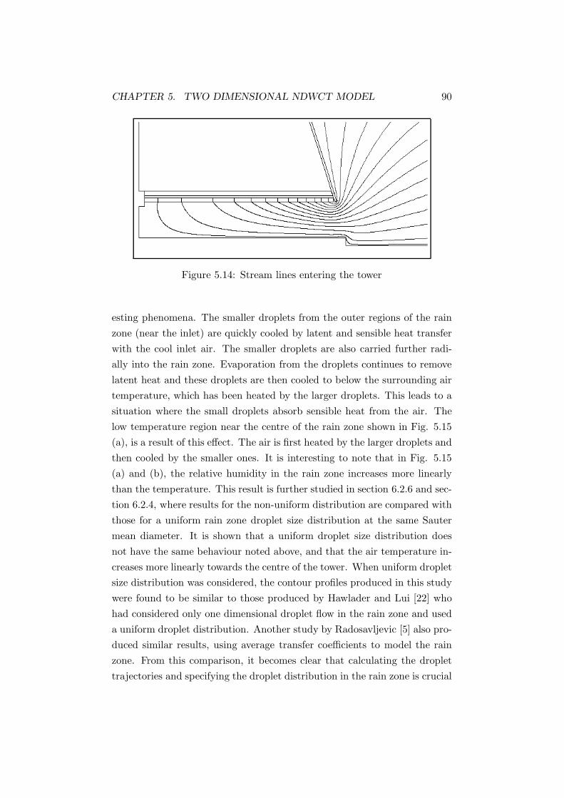
CHAPTER 5. TWO DIMENSIONAL NDWCT MODEL 90
Figure 5.14: Stream lines entering the tower
esting phenomena. The smaller droplets from the outer regions of the rain
zone (near the inlet) are quickly cooled by latent and sensible heat transfer
with the cool inlet air. The smaller droplets are also carried further radi-
ally into the rain zone. Evaporation from the droplets continues to remove
latent heat and these droplets are then cooled to below the surrounding air
temperature, which has been heated by the larger droplets. This leads to a
situation where the small droplets absorb sensible heat from the air. The
low temperature region near the centre of the rain zone shown in Fig. 5.15
(a), is a result of this effect. The air is first heated by the larger droplets and
then cooled by the smaller ones. It is interesting to note that in Fig. 5.15
(a) and (b), the relative humidity in the rain zone increases more linearly
than the temperature. This result is further studied in section 6.2.6 and sec-
tion 6.2.4, where results for the non-uniform distribution are compared with
those for a uniform rain zone droplet size distribution at the same Sauter
mean diameter. It is shown that a uniform droplet size distribution does
not have the same behaviour noted above, and that the air temperature in-
creases more linearly towards the centre of the tower. When uniform droplet
size distribution was considered, the contour profiles produced in this study
were found to be similar to those produced by Hawlader and Lui [22] who
had considered only one dimensional droplet flow in the rain zone and used
a uniform droplet distribution. Another study by Radosavljevic [5] also pro-
duced similar results, using average transfer coefficients to model the rain
zone. From this comparison, it becomes clear that calculating the droplet
trajectories and specifying the droplet distribution in the rain zone is crucial

CHAPTER 5. TWO DIMENSIONAL NDWCT MODEL 91
to achieving an accurate representation of the heat and mass transfer in the
tower.
The contours of pressure in Fig. 5.15 (d) and Fig. 5.16 (d) show that
in the rain zone, with the exception of a small area near the inlet, the
pressure distribution across the tower is nearly uniform. This suggests that
the resistance to air flow from the water flow in the rain zone is relatively
minor and the major resistance to flow is through the fill. This result is
similar to that in the study by Hawlader and Liu [22].
The small low pressure region below the fill can be explained by exam-
ining the contours of air speed. The air speed is highest just below the
tower lip as shown in Fig. 5.15 (c) and Fig. 5.16 (c). This low pressure
region retards the air flow into the fill in this region, but does not generate
a re-circulation zone in the fill as shown in the vector plots. Further into
the rain zone, the flow decelerates as it is drawn up into the tower (see Fig.
5.13). The magnitude of the velocity in the fill appears to be very uniform
across the tower except for the region near the tower inlet and at the centre
of the tower.
The dramatic decrease in the velocity of air moving through the fill in
the inlet effected region leads to an important concern with the validity of
the empirical correlations for the transfer coefficient and the loss coefficient.
These relations are functions of the air mass flux and are only valid over the
range of experimental data to which they are correlated. In this case, the
correlations are valid for 1.2kg/s/m2 < Ga < 4.2kg/s/m2 [3, 61, 102]. Near
the inlet, the air mass flux decreases to less than 0.8kg/s/m2, considerably
below the valid range.
In Chapter 6 the model described in this chapter has been used to sim-
ulate the tower performance for a range of tower inlet heights, fill depths
and water flow rates. To contribute to the current discussion, the plots of
the Poppe Merkel number and fill loss coefficient for these simulations have
been presented here in Figs. 5.17 and 5.18. These plots show how the co-
efficients vary across the tower, from the inlet to the centre of the tower.
For all the parameters shown, the plots show the nearly uniform profile of
the loss coefficient and Poppe Merkel number across the tower except for
the inlet affected region. Here the loss coefficient rises sharply and Poppe
Merkel number decreases. Fortunately however, the region over which the
majority of the spike/drop occurs is very small and has a negligible effect on
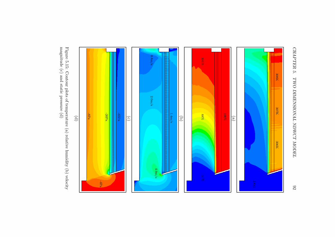
CH
AP
TE
R5.
TW
OD
IME
NSIO
NA
LN
DW
CT
MO
DE
L92
(a)
(b)
(c)
(d)
Figu
re5.15:
Con
tour
plots
oftem
peratu
re(a)
relativehum
idity
(b)
velocity
magn
itude
(c)an
dstatic
pressu
re(d
)
295K
306K
307K
308K
55%
100%
100%
88%
0.8
m/s
2.0
m/s
4.9
m/s
1.4
m/s
-65Pa
-26Pa
-8Pa
-4Pa

CH
AP
TE
R5.
TW
OD
IME
NSIO
NA
LN
DW
CT
MO
DE
L93
(a)(b
)
(c)(d
)
Figu
re5.16:
Con
tour
plots
oftem
peratu
re(a)
relativehum
idity
(b)
velocity
magn
itude
(c)an
dstatic
pressu
re(d
)
55%
100%
100%
0Pa
-65Pa
-23Pa
0m
/s
0.8
m/s
3.0
m/s
295K
307K

CHAPTER 5. TWO DIMENSIONAL NDWCT MODEL 94
the solution. In the region where this is a concern, the loss coefficient has
been arbitrarily limited to Kfi < 40. No limiter was placed on the Poppe
Merkel number as this is less severely effected. The effect of the value to
which loss coefficient is limited has been tested and found to be negligible.
In all simulations this was monitored closely.
5.12 Conclusions
An axisymmetric model has been developed and partially validated against
manufacturers’ cooling tower data. The model has been shown to be in-
sensitive to the parameters which are less certain in the model, such as the
specification of initial droplet velocities in the rain and spray zone and the
loss coefficients of the drift eliminators and tower supports. The heat and
mass transfer routine used to model the fill has been compared with an im-
plementation of the Poppe model and was found to give excellent results.
Excluding the effects of condensation is demonstrated to have a significant
effect on the predictions of the air temperature.
The simulation results compare well with previous work by Hawlader
and Liu [22]. Differences in the air temperature predicted in this study and
that predicted by Hawlader and Liu [22] can be explained by improvements
in the representation of droplet flow in the rain zone in this study. The air
flow in the fill is almost uniform across the tower with the exception of a
small region strongly affected by the flow through the tower inlet. Here,
the air flow in the fill is significantly reduced but no re-circulation zone is
generated.

CHAPTER 5. TWO DIMENSIONAL NDWCT MODEL 95
0
0.2
0.4
0.6
0.8
1
1.2
1.4
1.6
0 5 10 15 20 25 30 35 40 45 50
Me p
Radius (m)
depth = 0.6mdepth = 0.9mdepth = 1.2m
(a)
0
0.2
0.4
0.6
0.8
1
1.2
1.4
0 5 10 15 20 25 30 35 40 45 50
Me p
Radius (m)
inlet height = 8.577minlet height = 6.777minlet height = 4.977m
(b)
0
0.2
0.4
0.6
0.8
1
1.2
1.4
0 5 10 15 20 25 30 35 40 45 50
Me P
Radius (m)
12500kg/s15000kg/s22500kg/s30000kg/s
(c)
Figure 5.17: Radial profile of fill Poppe Merkel number with fill depth (a),inlet height (b) and water flow rate (c).
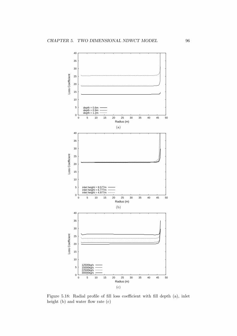
CHAPTER 5. TWO DIMENSIONAL NDWCT MODEL 96
0
5
10
15
20
25
30
35
40
0 5 10 15 20 25 30 35 40 45 50
Loss
Coe
ffici
ent
Radius (m)
depth = 0.6mdepth = 0.9mdepth = 1.2m
(a)
0
5
10
15
20
25
30
35
40
0 5 10 15 20 25 30 35 40 45 50
Loss
Coe
ffici
ent
Radius (m)
inlet height = 8.577minlet height = 6.777minlet height = 4.977m
(b)
0
5
10
15
20
25
30
35
40
0 5 10 15 20 25 30 35 40 45 50
Loss
Coe
ffici
ent
Radius (m)
12500kg/s15000kg/s22500kg/s30000kg/s
(c)
Figure 5.18: Radial profile of fill loss coefficient with fill depth (a), inletheight (b) and water flow rate (c)

Chapter 6
Sensitivity of Key Tower
Design and Operating
Parameters
6.1 Introduction
The influence of a range of design parameters on the performance of a stan-
dard NDWCT design is explored in this chapter. The base case for this
investigation has a tower height of 131m, fill base diameter of 98m, total
water flow rate of 15,000kg/s at 313K, a tower inlet height of 8.577m and a
fill depth of 1.0m (see Table 5.1). Here additional fill depths of 1.2m, 0.9m
and 0.6m were tested, along with water flow rates of 12,500kg/s, 22,500kg/s
and 30,000kg/s and tower inlet heights of 6.777m and 4.977m. Of particular
interest in this investigation is the non-uniformity of heat and mass transfer
across the tower, something which has not been well examined in literature.
It provides the basis for understanding of one dimensional model limitations
as discussed in Chapter 7 and further optimisation as discussed in Chapter
8.
6.2 Results
The following plots (Figs. 6.1-6.18) examine the variation in relevant flow
quantities through the tower (Fig. 5.1). The plots can be viewed as an
axisymmetric section with the centre of the tower at a radius of 0m and the
97

CHAPTER 6. SENSITIVITY OF KEY PARAMETERS 98
tower inlet located at a radius of 46.8m. The heat and mass transfer regions
extend from the tower inlet to the causeway at a radius of 1.4m.
6.2.1 Reference conditions
The radial profiles detailing tower performance under the reference tower
parameters are shown in Figs. 6.1-6.3 with the water flow rate of 15, 000kg/s
or in Figs. 6.8-6.10 with the inlet height of 8.577m.
An examination of the axial air mass flux profile (Ga) in the fill (Fig.
6.1 (a)) reveals that the profile is largely uniform across the radius with
values between 1.7 and 1.8kg/s/m2. At the inlet the air mass flux decreases
sharply to less than 0.9kg/s/m2. This abrupt reduction in performance is
due to the low pressure region below the tower inlet retarding the driving
force for flow through the fill (see section 5.11).
Fig. 6.1 (b) gives the temperature of the water as it passes axially down
through the heat transfer zones. The first axial location is the top surface of
the fill, which is the fill water inlet (Fig. 5.1). The water passes through the
fill to the fill water outlet and then through the rain zone to the collection
pond or basin. The water temperature increases almost linearly towards the
centre of the tower. The maximum radial variation in basin temperature is
6K, which is large compared with the overall tower range of 13.5K. Near the
tower inlet, the lower airflow in the fill causes the water outlet temperature
to rise from 298K to 300K.
The water is evenly distributed across the fill at 2.21kg/s/m2 but the
axisymmetric geometry means that there is more fill area per metre radius at
the tower’s outer edge than at the tower centre. The outer 7m of the tower
delivers more than 30% of the total cooling compared with the inner 15m
which delivers less than 10% of the cooling. It should be noted however that
although the inlet losses occur at a critical position, most of the temperature
spike only occurs over the very last portion of the tower, less than 1.0m.
Eliminating this loss from the tower therefore would have a very minor
effect. Removing the temperature spike from the data in Fig. 6.1 (b) and
re-calculating the Trange with the temperature in the inlet effected region
maintained at the minimum basin temperature, results in an improvement
in overall cooling range of less than 0.06K.
Fig. 6.2 (a) shows how the local cooling load is distributed between
the spray, fill and rain zones. The fill region accounts for more than 70%

CHAPTER 6. SENSITIVITY OF KEY PARAMETERS 99
0.6
0.8
1
1.2
1.4
1.6
1.8
2
0 5 10 15 20 25 30 35 40 45 50
Dry
Air
Mas
s F
lux
(kg/
s/m
2 )
Radius (m)
12,500kg/s (αk≈ 1.02)15,000kg/s (αk ≈ 1.02)22,500kg/s (αk ≈ 1.01)30,000kg/s (αk ≈ 1.00)
(a)
296
298
300
302
304
306
308
310
312
0 5 10 15 20 25 30 35 40 45 50
Wat
er T
empe
ratu
re (
K)
Radius (m)
Tower Water Inlet Temperature = 313K
Fill Water Inlet
Fill Water Outlet
Basin15,000kg/s22,500kg/s30,000kg/s
(b)
294
296
298
300
302
304
306
308
310
312
0 5 10 15 20 25 30 35 40 45 50
Air
Tem
pera
ture
(K
)
Radius (m)
Fill Air Inlet
Fill Air Outlet
12,500kg/s15,000kg/s22,500kg/s30,000kg/s
(c)
Figure 6.1: Radial profile of air mass flux in the fill (a), water temperature(b) and air temperature (c) with variable water flow rate, a fill depth of1.0m and a tower inlet height of 8.577m

CHAPTER 6. SENSITIVITY OF KEY PARAMETERS 100
0
20
40
60
80
100
0 5 10 15 20 25 30 35 40 45 50
% W
ater
Tem
pera
ture
Dro
p pe
r Z
one
Radius (m)
Rain Zone (%)
Fill Zone (%)
Spray Zone (%)
12,500kg/s15,000kg/s22,500kg/s30,000kg/s
(a)
0
20
40
60
80
100
120
140
160
180
200
0 5 10 15 20 25 30 35 40 45 50
Ga
(i ma,
o -
i ma,
i) (k
W/m
2 )
Radius (m)
Fill Air Outlet
Fill Air Inlet12500kg/s15000kg/s22500kg/s30000kg/s
(b)
10
20
30
40
50
60
70
0 5 10 15 20 25 30 35 40 45 50
Cp w
(T
w,i-
Tw
,o)
(kW
/kg
wat
er)
Radius (m)
12,500kg/s15,000kg/s22,500kg/s30,000kg/s
(c)
Figure 6.2: Radial profile of local water temperature drop per zone (a),cumulative heat transfer to air (b) and local cooling load (c) with variablewater flow rate, a fill depth of 1.0m and a tower inlet height of 8.577m

CHAPTER 6. SENSITIVITY OF KEY PARAMETERS 101
0.005
0.01
0.015
0.02
0.025
0.03
0.035
0.04
0.045
0.05
0 5 10 15 20 25 30 35 40 45 50
ω
Radius (m)
Fill Air Inlet
Fill Air Outlet
12500kg/s15000kg/s22500kg/s30000kg/s
Figure 6.3: Radial profile of specific humidity at the fill inlet with variablewater flow rate, a fill depth of 1.0m and a tower inlet height of 8.577m
of the cooling range and the spray region less than 10%. The rain zone
accounts for just over 20% of the local cooling range through most of the
tower but at the tower inlet, it rises to almost 40%, where the high speed
airflow at the inlet improves the heat transfer in the rain region, somewhat
counteracting the poorer performance of the fill in this region. The radial
profile of the local cooling load per kg water flow (Cpw(Tw,i−Tw,o)) is given
in Fig. 6.2 (c). The largely uniform axial air flow through the fill suggests
that the non-uniform water outlet temperature and local cooling load profile
is largely a function of the air temperature and humidity as it enters the
fill. The air temperature at the centre of the tower is almost 6K warmer
than the ambient air at the inlet (Fig. 6.1 (c)). The humidity also increases
significantly through the rain zone (Fig. 6.3), reducing the driving force for
heat transfer at the centre of the tower. This non-uniformity of heat transfer
can be seen clearly in Fig. 6.2 (b), where the total heat transfered to the
air from the tower inlet to the fill inlet and then to the fill outlet is plotted
per unit fill area (Ga(ima,o − ima,i)).
The profiles of the specific humidity across the tower, both at the inlet
to the fill and at the top of the fill can be seen in Fig. 6.3. The interesting
phenomena noted in section 5.11, where the humidity increases faster than
the air temperature due to the non-uniform droplet distribution, can be
seen in this figure. In Fig. 6.1 (c) the air temperature increases very slowly

CHAPTER 6. SENSITIVITY OF KEY PARAMETERS 102
through the outer rain region whereas the specific humidity profile in Fig.
6.3 shows that the evaporation increases almost linearly throughout the rain
zone. This is further discussed in secion 6.2.6.
6.2.2 Water flow rate
The reference cooling tower has a water flow rate of 15, 000kg/s (mas flux
of 2.21kg/s/m2). The tower also comes with design curves for a water flow
rate of 12, 500kg/s (1.8kg/s/m2). Here two additional cases of 22, 500kg/s
(3.3kg/s/m2) and 30, 000kg/s (4.4kg/s/m2) water flow rate have been con-
sidered. The additional cases may be unreasonably large for cooling tower
design but they do provide some insight into the model sensitivities. The fill
loss coefficient and transfer coefficient correlations used in this study, were
developed with water flow rates between (2.7kg/s/m2) and (6.1kg/s/m2)
[102].
The dry air mass flux in the fill is shown together with the corresponding
kinetic energy coefficient in Fig. 6.1 (a). The kinetic energy coefficient, αk,
is calculated as,
αk =1
V 3aveA
∫V 3dA, (6.1)
where Vave = 1A
∫V dA. Increasing the water flow rate increases number of
droplets in the rain zone and therefore increases the resistance to air flow
through the rain zone. This reduces the radial air flow to the centre of the
tower. It also has the effect of reducing the strength of the low pressure zone
below the tower inlet resulting in a small increase in the axial flow of air
into the fill in this region. Thermally, the effect of the inlet affected region is
also reduced at higher water flow rates as is evidenced by the smaller rise in
water temperature at the tower inlet, the absence of a large increase in rain
zone load fraction in Fig. 6.2 (a) and an overall decrease in local cooling
load in Fig. 6.2 (c).
Increasing the water flow rate increases the thermal mass of the water
and has the effect of redistributing the heat transfer radially out towards
the tower inlet and axially down towards the rain zone. The water tem-
perature profile (Fig. 6.1 (b)) shows a basin water temperature gradient
of less than 6K between the tower inlet and centre at 15, 000kg/s. This
rises to almost 9.5K at 30, 000kg/s. Higher water flow rates lead to a large
radial redistribution of the cooling in the tower as the air in the rain zone

CHAPTER 6. SENSITIVITY OF KEY PARAMETERS 103
is heated severely towards the tower centre (Fig. 6.1 (c)) and the air flow is
also slightly reduced in this region. The radial re-distribution of cooling in
the tower is also well shown in Fig. 6.2 (c), with a more pronounced cooling
load gradient from tower centre to tower inlet. The axial re-distribution of
the cooling load from the fill to the rain zone at higher water flow rates can
best be seen in Fig. 6.2 (a). At a flow rate of 15, 000kg/s, the rain zone
contributes around 20% of the local cooling range whereas at 30, 000kg/s,
it rises to almost 40%. At higher water flow rates, the heat and mass trans-
fer is greater in the rain zone. Hence the air entering the fill is at higher
temperature and humidity which results in a proportional reduction in heat
and mass transfer in this region.
6.2.3 Fill depth
Three fill depths have been tested, 0.6m, 0.9m and 1.2m. Varying the fill
height over this range does not introduce any significant change to the non-
uniformity of the air flow (Fig. 6.4 (a)), the water outlet temperature (Fig.
6.4 (b)) or the cooling load distribution (Fig. 6.5 (a-c)). The deeper fill
has a more uniform air-flow profile due to the increased flow restriction in
the tower. At low fill depths the air flow increases slightly to the centre,
increasing the kinetic energy coefficient from 1.01 at a fill depth of 1.2m to
1.03 at a fill depth of 0.6m.
The axial distribution of cooling load between the spray, fill and rain
zones is also fairly constant, although at 0.6m fill depth the rain zone starts
to occupy a higher percentage of the total cooling. This is because the water
entering the rain zone is at a higher temperature so the heat transfer here
improves and this region becomes relatively more effective (Fig. 6.5 (a)).
This gives some insight into the effect of an optimal fill depth selection.
There is very little increase in cooling load seen between a fill depth of 0.9m
and 1.2m. At a depth of 0.6m however, the fill is insufficiently sized such
that a small increase in fill depth returns a large increase in water cooling.
6.2.4 Tower inlet height
Here three inlet heights are examined, 8.577m, 6.777m and 4.977m. The
reference design height is 8.577m. Reducing the tower inlet height reduces
the flow area into the tower, increasing the flow restriction and increasing
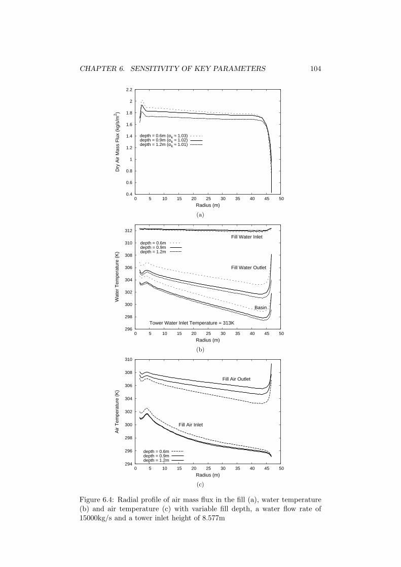
CHAPTER 6. SENSITIVITY OF KEY PARAMETERS 104
0.4
0.6
0.8
1
1.2
1.4
1.6
1.8
2
2.2
0 5 10 15 20 25 30 35 40 45 50
Dry
Air
Mas
s F
lux
(kg/
s/m
2 )
Radius (m)
depth = 0.6m (αk ≈ 1.03)depth = 0.9m (αk ≈ 1.02)depth = 1.2m (αk ≈ 1.01)
(a)
296
298
300
302
304
306
308
310
312
0 5 10 15 20 25 30 35 40 45 50
Wat
er T
empe
ratu
re (
K)
Radius (m)
Tower Water Inlet Temperature = 313K
Fill Water Inlet
Fill Water Outlet
Basin
depth = 0.6m depth = 0.9m depth = 1.2m
(b)
294
296
298
300
302
304
306
308
310
0 5 10 15 20 25 30 35 40 45 50
Air
Tem
pera
ture
(K
)
Radius (m)
Fill Air Inlet
Fill Air Outlet
depth = 0.6mdepth = 0.9mdepth = 1.2m
(c)
Figure 6.4: Radial profile of air mass flux in the fill (a), water temperature(b) and air temperature (c) with variable fill depth, a water flow rate of15000kg/s and a tower inlet height of 8.577m

CHAPTER 6. SENSITIVITY OF KEY PARAMETERS 105
0
20
40
60
80
100
0 5 10 15 20 25 30 35 40 45 50
% W
ater
Tem
pera
ture
Dro
p pe
r Z
one
Radius (m)
Rain Zone (%)
Fill Zone (%)
Spray Zone (%)
depth = 0.6mdepth = 0.9mdepth = 1.2m
(a)
0
20
40
60
80
100
120
140
160
0 5 10 15 20 25 30 35 40 45 50
Ga
(i ma,
o -
i ma,
i) (k
W/m
2 )
Radius (m)
Fill Air Outlet
Fill Air Inlet
fill depth = 0.6mfill depth = 0.9mfill depth = 1.2m
(b)
30
35
40
45
50
55
60
65
70
0 5 10 15 20 25 30 35 40 45 50
Cp w
(T
w,i-
Tw
,o)
(kW
/kg
wat
er)
Radius (m)
depth = 0.6mdepth = 0.9mdepth = 1.2m
(c)
Figure 6.5: Radial profile of local water temperature drop per zone (a),cumulative heat transfer to air (b) and local cooling load (c) with variablefill depth, a water flow rate of 15000kg/s and a tower inlet height of 8.577m

CHAPTER 6. SENSITIVITY OF KEY PARAMETERS 106
0.005
0.01
0.015
0.02
0.025
0.03
0.035
0.04
0 5 10 15 20 25 30 35 40 45 50
ω
Radius (m)
Fill Air Outlet
Fill Air Inlet
fill depth 0.6mfill depth 0.9mfill depth 1.2m
Figure 6.6: Radial profile of specific humidity with variable fill depth, awater flow rate of 15000kg/s and a tower inlet height of 8.577m
the air velocity beneath the fill. The radial velocity of the air entering the
tower at the inlet is given in Fig. 6.7. The maximum velocity of the flow
at an inlet height of 4.977m is ∼ 50% larger than that at an inlet height of
8.577m. This has the effect of further decreasing the pressure below the fill
at the inlet which further retards the axial flow into the fill in this region
(Fig. 6.8 (a)). The kinetic energy coefficient rises from 1.02 at an inlet
height of 8.577m to 1.05 at an inlet height of 4.977m. The size of the inlet
effected region remains almost the same at approximately 3.5m of the radius
under all cases tested (Fig. 6.8 (b)). Although the performance degradation
in this region does increase a little with reduced inlet height, the overall
effect of the region remains negligible. If the effect of the inlet was removed
and the temperature maintained at the minimum basin temperature, the
overall water outlet temperature would be reduced by only 0.14K for the
4.977m case and by 0.06K for the 8.577m case.
Surprisingly, the load fraction in the rain zone does not change much with
inlet height, with the heat transfer reduced in equal proportion through all
the heat transfer zones. Initial expectations were that the reduced droplet
residence time in the rain zone, due to the lower rain zone, would lead to
severely reduced rain zone performance. The combination of the higher
air velocity through the rain zone and the poorer performance on the other
regions in the tower (due to lower overall air flow rate), means the proportion

CHAPTER 6. SENSITIVITY OF KEY PARAMETERS 107
0 0.25 0.5 0.75 1U/U
max
0
0.2
0.4
0.6
0.8
1
y/h
height = 4.977mheight = 6.777mheight = 8.577m
Figure 6.7: Radial velocity magnitude at the tower inlet with r = 46.5m,where Umax = 6.5(m/s) for h = 4.977m, Umax = 5.55(m/s) for h = 6.777mand Umax = 5.0(m/s) for h = 8.577m

CHAPTER 6. SENSITIVITY OF KEY PARAMETERS 108
0.2
0.4
0.6
0.8
1
1.2
1.4
1.6
1.8
2
0 5 10 15 20 25 30 35 40 45 50
Dry
Air
Mas
s F
lux
(kg/
s/m
2 )
Radius (m)
inlet height = 8.577m (αk≈ 1.02)inlet height = 6.777m (αk≈ 1.03)inlet height = 4.977m (αk≈ 1.05)
(a)
296
298
300
302
304
306
308
310
312
0 5 10 15 20 25 30 35 40 45 50
Wat
er T
empe
ratu
re (
K)
Radius (m)
Tower Water Inlet Temperature = 313K
Fill Water Inlet
Fill Water Outlet
Basin
inlet height = 8.577minlet height = 6.777minlet height = 4.977m
(b)
294
296
298
300
302
304
306
308
310
312
0 5 10 15 20 25 30 35 40 45 50
Air
Tem
pera
ture
(K
)
Radius (m)
Fill Air Inlet
Fill Air outlet
inlet height = 8.577minlet height = 6.777minlet height = 4.977m
(c)
Figure 6.8: Radial profile of air mass flux in the fill (a), water temperature(b) and air temperature (c) with variable tower inlet height, a water flowrate of 15000kg/s and a fill depth of 1.0m

CHAPTER 6. SENSITIVITY OF KEY PARAMETERS 109
0
20
40
60
80
100
0 5 10 15 20 25 30 35 40 45 50
% W
ater
Tem
pera
ture
Dro
p pe
r Z
one
Radius (m)
Rain Zone (%)
Fill Zone (%)
Spray Zone (%)
inlet height = 8.577minlet height = 6.777minlet height = 4.977m
(a)
0
20
40
60
80
100
120
140
160
0 5 10 15 20 25 30 35 40 45 50
Ga
(i ma,
o -
i ma,
i) (k
W/m
2 )
Radius (m)
Fill Air Outlet
Fill Air Inlet
inlet height = 8.577minlet height = 6.777minlet height = 4.977m
(b)
30
35
40
45
50
55
60
65
0 5 10 15 20 25 30 35 40 45 50
Cp w
(T
w,i-
Tw
,o)
(kW
/kg
wat
er)
Radius (m)
inlet height = 8.577minlet height = 6.777minlet height = 4.977m
(c)
Figure 6.9: Radial profile of local water temperature drop per zone (a),cumulative heat transfer to air (b) and local cooling load (c) with variabletower inlet height, a water flow rate of 15000kg/s and a fill depth of 1.0m
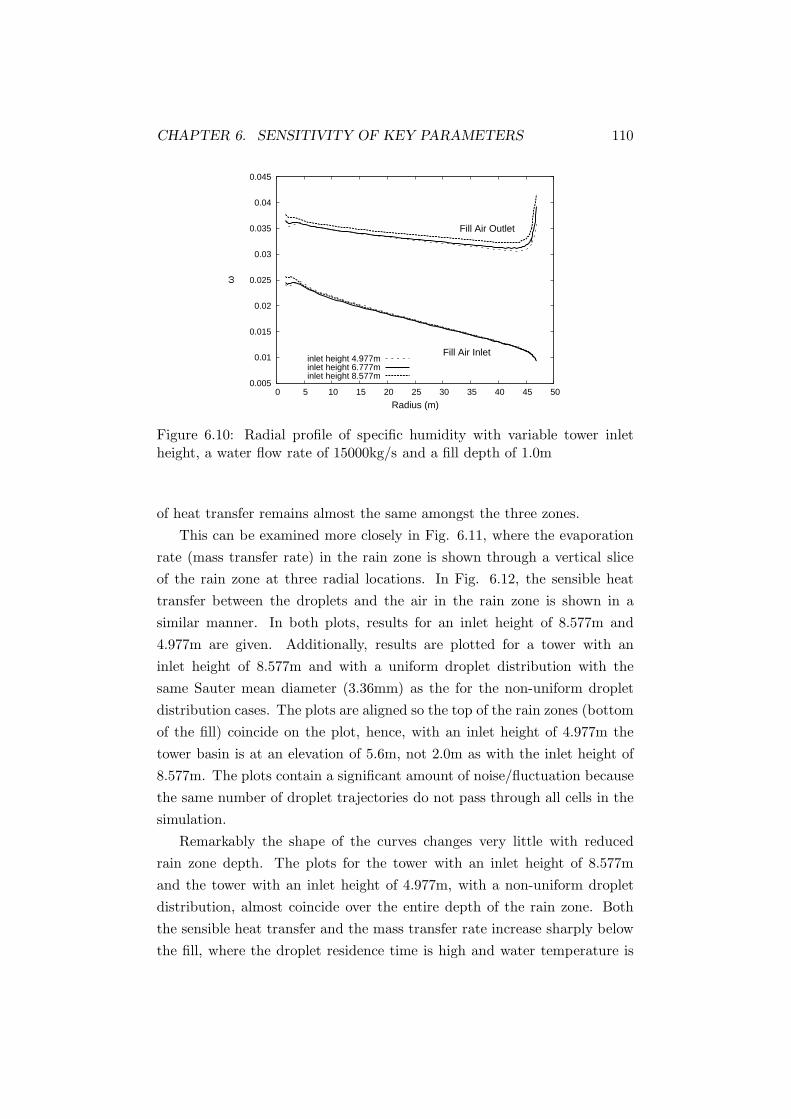
CHAPTER 6. SENSITIVITY OF KEY PARAMETERS 110
0.005
0.01
0.015
0.02
0.025
0.03
0.035
0.04
0.045
0 5 10 15 20 25 30 35 40 45 50
ω
Radius (m)
Fill Air Inlet
Fill Air Outlet
inlet height 4.977minlet height 6.777minlet height 8.577m
Figure 6.10: Radial profile of specific humidity with variable tower inletheight, a water flow rate of 15000kg/s and a fill depth of 1.0m
of heat transfer remains almost the same amongst the three zones.
This can be examined more closely in Fig. 6.11, where the evaporation
rate (mass transfer rate) in the rain zone is shown through a vertical slice
of the rain zone at three radial locations. In Fig. 6.12, the sensible heat
transfer between the droplets and the air in the rain zone is shown in a
similar manner. In both plots, results for an inlet height of 8.577m and
4.977m are given. Additionally, results are plotted for a tower with an
inlet height of 8.577m and with a uniform droplet distribution with the
same Sauter mean diameter (3.36mm) as the for the non-uniform droplet
distribution cases. The plots are aligned so the top of the rain zones (bottom
of the fill) coincide on the plot, hence, with an inlet height of 4.977m the
tower basin is at an elevation of 5.6m, not 2.0m as with the inlet height of
8.577m. The plots contain a significant amount of noise/fluctuation because
the same number of droplet trajectories do not pass through all cells in the
simulation.
Remarkably the shape of the curves changes very little with reduced
rain zone depth. The plots for the tower with an inlet height of 8.577m
and the tower with an inlet height of 4.977m, with a non-uniform droplet
distribution, almost coincide over the entire depth of the rain zone. Both
the sensible heat transfer and the mass transfer rate increase sharply below
the fill, where the droplet residence time is high and water temperature is

CHAPTER 6. SENSITIVITY OF KEY PARAMETERS 111
0 2 4 6 8 10 12Height (m)
0
0.001
0.002
0.003
0.004
0.005
0.006
Rat
e of
mas
s tr
ansf
er (
kg/s
/m3 )
inlet height = 8.577m (uniform diameter)inlet height = 8.577minlet height = 4.977m
(a)
0 2 4 6 8 10 12Height (m)
0
0.002
0.004
0.006
0.008
Rat
e of
mas
s tr
ansf
er (
kg/s
/m3 )
(b)
0 2 4 6 8 10 12Height (m)
0
0.002
0.004
0.006
0.008
0.01
Rat
e of
mas
s tr
ansf
er (
kg/s
/m3 )
(c)
Figure 6.11: Total mass transfer from droplets to the gas phase along avertical slice through the rain zone, at a radius of (a) 20m, (b) 30m and (c)40m
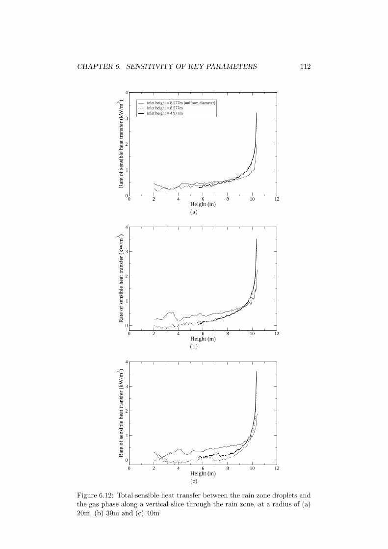
CHAPTER 6. SENSITIVITY OF KEY PARAMETERS 112
0 2 4 6 8 10 12Height (m)
0
1
2
3
4
Rat
e of
sen
sibl
e he
at tr
ansf
er (
kW/m
3 )
inlet height = 8.577m (uniform diameter)inlet height = 8.577minlet height = 4.977m
(a)
0 2 4 6 8 10 12Height (m)
0
1
2
3
4
Rat
e of
sen
sibl
e he
at tr
ansf
er (
kW/m
3 )
(b)
0 2 4 6 8 10 12Height (m)
0
1
2
3
4
Rat
e of
sen
sibl
e he
at tr
ansf
er (
kW/m
3 )
(c)
Figure 6.12: Total sensible heat transfer between the rain zone droplets andthe gas phase along a vertical slice through the rain zone, at a radius of (a)20m, (b) 30m and (c) 40m
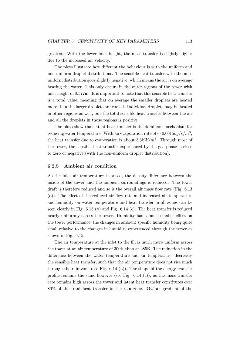
CHAPTER 6. SENSITIVITY OF KEY PARAMETERS 113
greatest. With the lower inlet height, the mass transfer is slightly higher
due to the increased air velocity.
The plots illustrate how different the behaviour is with the uniform and
non-uniform droplet distributions. The sensible heat transfer with the non-
uniform distribution goes slightly negative, which means the air is on average
heating the water. This only occurs in the outer regions of the tower with
inlet height of 8.577m. It is important to note that this sensible heat transfer
is a total value, meaning that on average the smaller droplets are heated
more than the larger droplets are cooled. Individual droplets may be heated
in other regions as well, but the total sensible heat transfer between the air
and all the droplets in those regions is positive.
The plots show that latent heat transfer is the dominant mechanism for
reducing water temperature. With an evaporation rate of ∼ 0.0015kg/s/m3 ,
the heat transfer due to evaporation is about 3.6kW/m3. Through most of
the tower, the sensible heat transfer experienced by the gas phase is close
to zero or negative (with the non-uniform droplet distribution).
6.2.5 Ambient air condition
As the inlet air temperature is raised, the density difference between the
inside of the tower and the ambient surroundings is reduced. The tower
draft is therefore reduced and so is the overall air mass flow rate (Fig. 6.13
(a)). The effect of the reduced air flow rate and increased air temperature
and humidity on water temperature and heat transfer in all zones can be
seen clearly in Fig. 6.13 (b) and Fig. 6.14 (c). The heat transfer is reduced
nearly uniformly across the tower. Humidity has a much smaller effect on
the tower performance, the changes in ambient specific humidity being quite
small relative to the changes in humidity experienced through the tower as
shown in Fig. 6.15.
The air temperature at the inlet to the fill is much more uniform across
the tower at an air temperature of 300K than at 285K. The reduction in the
difference between the water temperature and air temperature, decreases
the sensible heat transfer, such that the air temperature does not rise much
through the rain zone (see Fig. 6.14 (b)). The shape of the energy transfer
profile remains the same however (see Fig. 6.14 (c)), as the mass transfer
rate remains high across the tower and latent heat transfer constitutes over
80% of the total heat transfer in the rain zone. Overall gradient of the

CHAPTER 6. SENSITIVITY OF KEY PARAMETERS 114
0.6
0.8
1
1.2
1.4
1.6
1.8
2
2.2
2.4
2.6
0 5 10 15 20 25 30 35 40 45 50
Dry
Air
Mas
s F
lux
(kg/
s/m
2 )
Radius (m)
Ta = 285 RH40% (αk≈ 1.02)Ta = 300 RH40% (αk≈ 1.02)
Ta = 285 RH61.4% (αk≈ 1.02) Ta = 300 RH61.4% (αk≈ 1.02)
(a)
290
295
300
305
310
0 5 10 15 20 25 30 35 40 45 50
Wat
er T
empe
ratu
re (
K)
Radius (m)
Fill water inlet
Fill water outlet (Ta=285)
Fill water outlet (Ta=300)
Basin (Ta=285)
Basin (Ta=300)
Ta = 285 RH40%Ta = 300 RH40%
Ta = 285 RH61.4%Ta = 300 RH61.4%
(b)
285
290
295
300
305
310
0 5 10 15 20 25 30 35 40 45 50
Air
Tem
pera
ture
Radius (m)
Fill Air Inlet (Ta=285)
Fill Air Inlet (Ta=300)
Fill Air Outlet (Ta=285)
Fill Air Outlet (Ta=300)
Ta=285 RH40%Ta=300 RH40%
Ta=285 RH61.4%Ta=300 RH61.4%
(c)
Figure 6.13: Radial profile of air mass flux in the fill (a), water temperature(b) and air temperature (c) with variable ambient air temperature and hu-midity, a tower inlet height of 8.577m, a water flow rate of 15,000kg/s anda fill depth of 1.0m

CHAPTER 6. SENSITIVITY OF KEY PARAMETERS 115
0
20
40
60
80
100
0 5 10 15 20 25 30 35 40 45 50
% W
ater
Tem
pera
ture
Dro
p pe
r Z
one
Radius (m)
Rain Zone (%)
Fill Zone (%)
Spray Zone (%)
Ta = 285 RH40%Ta = 300 RH40%
Ta = 285 RH61.4%Ta = 300 RH61.4%
(a)
0
50
100
150
200
250
0 5 10 15 20 25 30 35 40 45 50
Ga
(i ma,
o -
i ma,
i) (k
W/m
2 )
Radius (m)
Fill air outlet
Fill air inlet
Ta=285 RH40%Ta=300 RH40%
Ta=285 RH61.4%Ta=300 RH61.4%
(b)
20
30
40
50
60
70
80
90
0 5 10 15 20 25 30 35 40 45 50
Cp w
(T
w,i-
Tw
,o)
(kW
/kg
wat
er)
Radius (m)
Ta = 285 RH40%Ta = 300 RH40%
Ta = 285 RH61.5%Ta = 300 RH61.5%
(c)
Figure 6.14: Radial profile of local water temperature drop per zone (a),cumulative heat transfer to air (b) and local cooling load (c) with variableambient air temperature and humidity, a tower inlet height of 8.577m, awater flow rate of 15,000kg/s and a fill depth of 1.0m

CHAPTER 6. SENSITIVITY OF KEY PARAMETERS 116
0
0.005
0.01
0.015
0.02
0.025
0.03
0.035
0.04
0 5 10 15 20 25 30 35 40 45 50
ω
Radius (m)
Fill Air Inlet
Fill Air Outlet
Ta = 285 RH40%Ta = 300 RH40%
Ta = 285 RH61.5%Ta = 300 RH61.5%
Figure 6.15: Radial profile of specific humidity with variable ambient airtemperature and humidity, a tower inlet height of 8.577m, a water flow rateof 15,000kg/s and a fill depth of 1.0m
air enthalpy profile remains the same regardless of inlet air temperature or
humidity. The limited effect the inlet conditions have on the mass transfer
profile can be seen in Fig. 6.15. The specific humidity profile remains much
the same across the tower regardless of inlet condition, it is just shifted due
to the change in air flow rate.
Overall, while the effect of ambient air temperature on performance is
significant, the effect of humidity or temperature on non-uniformity of heat
and mass transfer is minimal.
6.2.6 Droplet diameter
The droplet distribution in the rain zone for the reference tower, has a Sauter
mean diameter of 3.26mm (Table 5.3). Here results for the flow with uniform
droplet diameters of 3.26mm, 5.31mm and 7.31mm are also presented.
The droplet diameter is shown to have only a very slight impact on the
radial air-flow rate profile (Fig. 6.16 (a)), both overall and with respect to
any non-uniformity. Again, this is because the restriction through the fill
region dominates the flow.
The influence of droplet size on the heat and mass transfer however is
more significant. As the droplet diameter is increased, thereby reducing the

CHAPTER 6. SENSITIVITY OF KEY PARAMETERS 117
total wetted contact area, the heat and mass transfer in the rain zone is
reduced. The air undergoes less heating radially through the rain zone and
the air temperature and humidity at the centre of the tower are decreased
as shown in Fig. 6.16 (c) and Fig. 6.18. This has the effect of increasing the
cooling load in the centre of the tower (Fig. 6.17 (c)). Overall, the cooling
in the rain zone is increased from ∼10% for droplet diameter of 7.31mm and
more than 20% for the case with droplet diameters of 3.26mm.
It is interesting to note the differences in the results for the droplet di-
ameter of 3.26mm and the results for the non-uniform droplet distribution
with a Sauter mean diameter of 3.26mm, shown in Figs. 6.16-6.18. Overall
the tower performance is very similar. With the uniform droplet distribu-
tion, the tower range is 13.80 (K) and with the non-uniform distribution, the
tower range is 13.76 (K). The performance of the rain zone and the overall
non-uniformity of heat and mass transfer is very different however.
The most interesting feature is that the air temperature profiles are quite
different. The air temperature increases more linearly in the uniform droplet
diameter case (Fig. 6.18) than in the case with the droplet distribution, but
the profiles of specific humidity are quite similar. This is related to the
phenomena noted in section 5.11 and section 6.2.4, where the small water
droplets near the tower inlet are carried further into the tower and cool the
air in the rain zone. This is clearly seen in Fig. 6.19, in which the contours of
air temperature for the uniform droplet diameter case and the non-uniform
droplet distribution case are given. The cool region in the rain zone which
is observed in the case with the non-uniform droplet distribution, is absent
from the case with a uniform distribution. Additionally, the air temperature
in the rain zone clearly increases more uniformly across the tower for the
case with the uniform distribution. Overall, the proportion of heat and
mass transfer in the rain zone is slightly higher for the uniform distribution
as shown in Fig. 6.17 (a).
6.3 Conclusions
The results show that the air flow is quite uniform through the fill and
spray zones under the range of parameters considered in this study. The
flow appears to be strongly dominated by the resistance through the fill
region, including the spray zone and drift eliminators. Increasing the water

CHAPTER 6. SENSITIVITY OF KEY PARAMETERS 118
0.4
0.6
0.8
1
1.2
1.4
1.6
1.8
2
0 5 10 15 20 25 30 35 40 45 50
Dry
Air
Mas
s F
lux
(kg/
s/m
2 )
Radius (m)
droplet diameter = 3.26mm (αk≈ 1.02)droplet diameter = 5.31mm (αk≈ 1.03)droplet diameter = 7.31mm (αk≈ 1.03)Sauter diameter = 3.26mm (αk≈ 1.02)
(a)
296
298
300
302
304
306
308
310
312
0 5 10 15 20 25 30 35 40 45 50
Wat
er T
empe
ratu
re (
K)
Radius (m)
Tower Water Inlet Temperature = 313K
Fill Water Inlet
Fill Water Outlet
Basin
droplet diameter = 3.26mmdroplet diameter = 5.31mmdroplet diameter = 7.31mmSauter diameter = 3.26mm
(b)
294
296
298
300
302
304
306
308
310
0 5 10 15 20 25 30 35 40 45 50
Air
Tem
pera
ture
(K
)
Radius (m)
droplet diameter = 3.26mmdroplet diameter = 5.31mmdroplet diameter = 7.31mmSauter diameter = 3.26mm
(c)
Figure 6.16: Radial profile of air mass flux in the fill (a), water temperature(b) and air temperature (c) with variable droplet diameter in the rain zone,with a tower inlet height of 8.577m, a water flow rate of 15000kg/s and afill depth of 1.0m
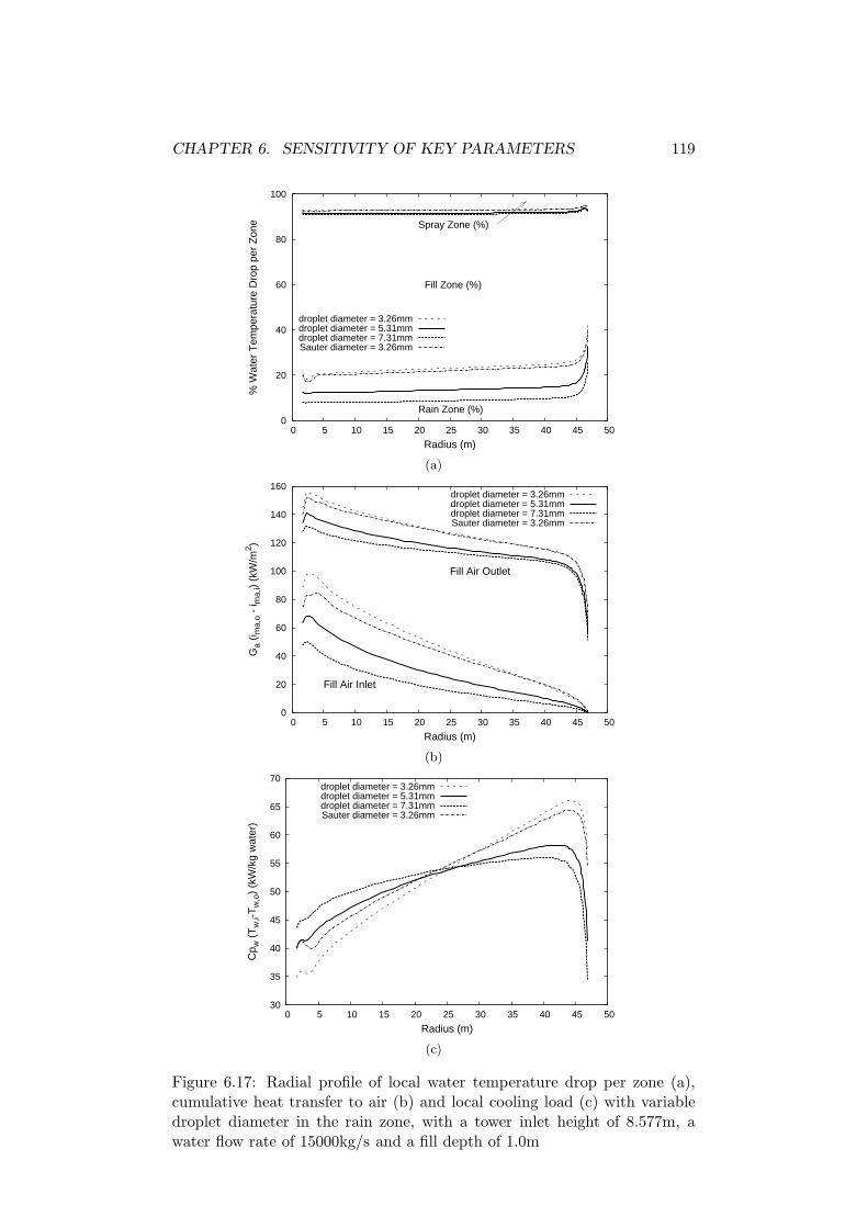
CHAPTER 6. SENSITIVITY OF KEY PARAMETERS 119
0
20
40
60
80
100
0 5 10 15 20 25 30 35 40 45 50
% W
ater
Tem
pera
ture
Dro
p pe
r Z
one
Radius (m)
Rain Zone (%)
Fill Zone (%)
Spray Zone (%)
droplet diameter = 3.26mmdroplet diameter = 5.31mmdroplet diameter = 7.31mmSauter diameter = 3.26mm
(a)
0
20
40
60
80
100
120
140
160
0 5 10 15 20 25 30 35 40 45 50
Ga
(i ma,
o -
i ma,
i) (k
W/m
2 )
Radius (m)
Fill Air Outlet
Fill Air Inlet
droplet diameter = 3.26mmdroplet diameter = 5.31mmdroplet diameter = 7.31mmSauter diameter = 3.26mm
(b)
30
35
40
45
50
55
60
65
70
0 5 10 15 20 25 30 35 40 45 50
Cp w
(T
w,i-
Tw
,o)
(kW
/kg
wat
er)
Radius (m)
droplet diameter = 3.26mmdroplet diameter = 5.31mmdroplet diameter = 7.31mmSauter diameter = 3.26mm
(c)
Figure 6.17: Radial profile of local water temperature drop per zone (a),cumulative heat transfer to air (b) and local cooling load (c) with variabledroplet diameter in the rain zone, with a tower inlet height of 8.577m, awater flow rate of 15000kg/s and a fill depth of 1.0m
CHAPTER 6. SENSITIVITY OF KEY PARAMETERS 120
0.005
0.01
0.015
0.02
0.025
0.03
0.035
0.04
0 5 10 15 20 25 30 35 40 45 50
ω
Radius (m)
Fill Air Inlet
Fill Air Outlet
droplet diameter = 3.26mmdroplet diameter = 5.31mmdroplet diameter = 7.31mmSauter diameter = 3.26mm
Figure 6.18: Radial profile specific humidity with variable droplet diameterin the rain zone, with a tower inlet height of 8.577m, a water flow rate of15000kg/s and a fill depth of 1.0m
flow rate or reducing the inlet height, increases the resistance to radial flow
through the rain zone but the effect is relatively minor. Even at the smallest
fill depth tested, the air flow was quite uniform across the tower.
In spite of the uniform air flow, there can be considerable non-uniformity
of heat transfer and water outlet temperature across the tower, with a 6K
variation in water outlet temperature from the tower centre to the tower inlet
at reference conditions. This is shown to be largely due to the cooling load
in the rain zone and the radial air flow there. High radial non-uniformity of
heat transfer across the tower can be expected when the cooling load in the
rain zone is high. Such a situation can arise with small rain zone droplet
sizes, low fill depths, high water flow rates and to a lesser extent large inlet
heights. While ambient temperature and humidity can have a significant
influence on overall performance, the results here show that large changes
in these parameters have very little effect on the non-uniformity of heat
transfer across the tower.
The results show that the effect of inlet height on radial non-uniformity of
heat transfer is surprisingly very small. Reducing the inlet height increases
flow restriction in the tower and reduces heat transfer almost uniformly
across the tower. The inlet affected region has been shown to have a minor
effect on performance except when inlet heights are very low. The inlet

CH
AP
TE
R6.
SE
NSIT
IVIT
YO
FK
EY
PA
RA
ME
TE
RS
121
(a)
(b)
Figu
re6.19:
Con
tours
ofair
temperatu
refor
drop
letdistrib
ution
with
Sau
term
eandiam
eterof
3.26mm
(a)an
dair
temperatu
refor
uniform
drop
letdis-
tribution
with
diam
eterof
3.26mm
(b)
295K
299K
306K
309K
295K
297K
306K
308K
CHAPTER 6. SENSITIVITY OF KEY PARAMETERS 122
affected region was shown to cause an overall water temperature rise of only
0.14K at an inlet height of 4.977m. Furthermore, the influence of inlet height
on the relative cooling load in the rain zone was shown to be minor. These
are significant results for optimisation studies, where reducing the tower
inlet height is desirable as it reduces the water pumping power requirements.
This work demonstrates that the inlet height may be significantly reduced
without any additional design problems from re-circulation zones or non-
uniform flow through the fill.
The heat and mass transfer in the rain zone is shown to be significantly
different for the case where there is a non-uniform droplet distribution in the
rain zone and the case when there is a uniform droplet distribution at the
same Sauter mean diameter. This difference is because when there is a non-
uniform droplet distribution, the small droplets take different trajectories
from the larger droplets and undergo different rates of cooling.

Chapter 7
One Dimensional Model
7.1 Introduction
In industry the majority of cooling tower design and optimisation is un-
dertaken using one dimensional models yet there is little work defining the
limitations of these models. As was shown in Chapter 6, there is a signif-
icant reduction in heat and mass transfer towards the centre of the tower
with a large gradient in water outlet temperature. The effects of these on
the predictions of simple one dimensional models are not well understood.
In this chapter, the numerical model presented in Chapter 5 is compared
with a one-dimensional model which does not solve for the flow field and
the predictions compared under a range of design conditions.
This chapter is arranged as follows. In section 7.2, previous work on the
development of the NDWCT one dimensional models has been reviewed.
In section 7.3, Kroger’s [1] one dimensional model has been described. In
section 7.5, the results of the comparison between the CFD model and the
one dimensional model are presented.
7.2 Previous work
Kroger’s [1] NDWCT modelling approach is the most detailed one dimen-
sional model in literature insofar as complete tower modelling is concerned.
Kroger and co-workers have contributed numerous publications on various
aspects of tower design and modelling [1, 12, 18–20, 32, 33, 52, 55, 61, 102,
104–108]. In Kroger’s model [1], the heat and mass transfer in the rain zone
123

CHAPTER 7. ONE DIMENSIONAL MODEL 124
is taken as a bulk averaged value in a similar manner to the fill. Hoffman
and Kroger [105] proposed the first semi-empirical transfer coefficient to ac-
count for the part cross-flow, part counterflow air/water flow in this region
which was later improved by de Villers and Kroger [20]. This is the only
correlation available in the literature and allows the rain zone to be treated
as an extension of the fill in the Merkel model. In essence, this method
assumes that the enthalpy of the air/water vapour mixture at the bottom of
the fill is uniform across the tower. For the spray zone, Kroger [1] correlated
Lowe and Christies’ spray data [7] in the format of the Merkel number (Eqn.
7.13).
The pressure losses that occur through the tower inlet, the contraction
into the tower fill, expansion losses out of the fill, and the losses as the
air stream exits the tower, are modelled in the same manner as the drift
eliminators, spray nozzles, tower supports and fill supports in the CFD
model. Much work has gone into developing empirical correlations for these
losses and understanding their interactions in a tower [1].
Lowe and Christie [7] used scale test models to determine the air velocity
profile across the tower and a loss coefficient for a number of shapes of
fill. The authors demonstrated that the resistance in an empty tower is
significant and is related to the ratio of the inlet height to the tower base
diameter. The authors stress the importance of ensuring an adequate inlet
height. The authors found that the loss coefficient of the system can be
found by adding the loss for the empty tower to the loss for the packing.
Terblanche and Kroger [107] conducted a model study and expressed
the inlet loss coefficients in terms of the height to diameter ratio and the
heat-exchanger/fill loss coefficient. The authors also showed that there is a
significant reduction in inlet losses when the lip of the shell inlet is rounded.
The author gives an empirical relation for the effective area as a function of
base diameter and inlet height. de Villers and Kroger [104] later advanced
the work with further experimental model studies and a CFD analysis. The
authors determined the influence of the rain zone on the inlet loss coefficient
and derived an empirical relationship.
Kroger [1] gives a complete compilation of available loss coefficients and
discussion on the topic.

CHAPTER 7. ONE DIMENSIONAL MODEL 125
7.3 One dimensional model
The one dimensional model presented here is based on Kroger’s [1] and
Kloppers’ [3] models. These models are obtained in the form of a heat
and mass transfer system coupled with a simple hydraulic flow calculation
where the system losses are represented with loss coefficients. These are
shown schematically in Fig. 7.1. Here the driving force for air flow is the
tower draft calculated simply as,
∆P = (ρ∞ − ρa,o)gHtower =n∑
i=1
KiρV 2
2, (7.1)
where the density ρ, the velocity V and the loss coefficients (Ki) are referred
to fill inlet conditions in the manner described in [1], thereby allowing the
coefficients to be summed. This simple model neglects an atmospheric lapse
rate but the CFD model used here has the same simplification so the models
are equivalent in this respect. The calculation of the air mass flow rate is
discussed in more detail in Appendix C.
The loss coefficients for the cooling tower shell supports, the water dis-
tribution piping network and the drift eliminators are the same as those em-
ployed in the CFD model in Chapter 5 (Kcts = 0.5, Kwdn = 0.5, Kfs = 0.5
and Kde = 3.5) as taken from [1]. In addition the tower inlet losses and
rain and spray zone losses are represented using the correlations described
in Kloppers thesis [3] and the citations therein. These are described in the
following sections.
The Merkel heat transfer method has been implemented here in the one
dimensional model, as the transfer characteristics for the rain and spray
zones are only available for the Merkel model and not the Poppe model.
The fill transfer coefficients for the Poppe model used in the CFD model are
derived from the same experimental data [3] as the Merkel transfer correla-
tions below (Eqns. 7.2-7.5). When implemented in the appropriate model
they produce the same result. The loss coefficients below (Eqns. 7.6 - 7.8)
are dissimilar to the Poppe loss coefficients in Chapter 5 as the air density
and fluid properties used to interpret the data are dependent on the heat
and mass transfer model used and so are different in each case [3].

CHAPTER 7. ONE DIMENSIONAL MODEL 126
1 2
3
4
Figure 7.1: Schematic representation of tower with flow resistance repre-sented as loss coefficients at locations: (1) = Kcts, (2) = Kct + Krz + Kfs,(3) = Kctc + Kfi + Kcte + Ksp + Kwdn + Kde and (4) = Kto
7.3.1 Fill transfer and loss coefficients
The following fill transfer coefficient correlations (Eqns. 7.2- 7.5) and loss
coefficient correlations (Eqns. 7.6 - 7.8) have been employed, all taken from
[3]. The correlations in Eqns. 7.2, 7.3 and 7.4 are used for fill depths of
0.6m, 0.9m and 1.2m respectively. In simulations of other fill depths, Eqn.
7.5 has been used.
Me0.6m
Lfi=
hmA
mwLfi
= 1.638988G0.282648w G0.682887
a
− 0.802755G0.560711w G0.644229
a (7.2)
Me0.9m
Lfi=
hmA
mwLfi
= 1.625618G0.091940w G0.702913
a
− 0.735958G0.376496w G0.6665399
a (7.3)

CHAPTER 7. ONE DIMENSIONAL MODEL 127
Me1.2m
Lfi=
hmA
mwLfi
= 1.357391G0.110577w G0.712196
a
− 0.567207G0.443165w G0.669846
a (7.4)
Megen
Lfi=
hmA
mwLfi= 1.019766G−0.432896
w G0.782744a L−0.292870
fi (7.5)
Similarly, the loss coefficient correlations in Eqns. 7.6, 7.7 and 7.8 have
been employed for simulations with fill depths 0.6m, 0.9m and 1.2m while
Eqn. 7.8 has been employed in the same manner as Eqn. 5.32 in Chapter 5.
Kfi,0.6m
Lfi= (0.00819G5.465533
w G−3.666315a
+17.545503G0.345860w G−0.036969
a ) (7.6)
Kfi,0.9m
Lfi= (1.633204G1.250268
w G−3.873083a
+16.170094G0.288861w G0.012429
a ) (7.7)
Kfi,1.2m
Lfi= (3.897830G0.777271
w G−2.114727a
+15.327472G0.215975w G0.079696
a ) (7.8)
Kfi,Lfi= Kfi,0.9mf + Kfi,1.2m(1 − f), (7.9)
where the smoothing factor f =(1.2−Lfi)(1.2−0.9) for 0.9 < Lfi < 1.2.
Kfi,Lfi= Kfi,0.6mf + Kfi,0.9m(1 − f), (7.10)
where the smoothing factor f =(0.9−Lfi)(0.9−0.6) for 0.6 < Lfi < 0.9.

CHAPTER 7. ONE DIMENSIONAL MODEL 128
7.3.2 Rain zone coefficients
The transfer coefficient and loss coefficient for the rain zone are given in
Eqn. 7.11 and Eqn. 7.12 respectively,
Merz = 12
(Dm
Vav,odd
)(Hi
dd
)(Pt
ρwoRvTai
)S0.33
c
×[(
lnws,Two + 0.622
wi + 0.622
)/(ws,Two − wi)
]
×[0.90757apρav,i − 30341.04aµµav − 0.37564
+4.04016
([0.55 + 41.7215(aLdd)
0.80043][0.713
+3.741(aLHi)−1.23456][3.11e(0.15 avVav,o) − 3.13]
exp[5.3759e(−0.2092aLHi)ln(0.3719e(0.0019055aL di)
+0.55)])]
, (7.11)
Krz = 3avVw,o(Hi/dd)
[0.2246 − 0.31467apρa + 5263.04aµµa
+0.775526(1.4824163exp(71.52aLdd) − 0.91)
×(0.39064exp(0.010912aLdi) − 0.17)
×(2.0892(avVav,o)−1.3944 + 0.14)
×exp
((0.8449log(aLdi/2) − 2.312)
×(0.3724log(avVav,o)
+0.7263)log(206.757(aLHi)−2.8344 + 0.43)
)], (7.12)
where aµ = 3.061 × 10⁻⁶(ρ4wg9
σw)0.25, ap = 998/ρw, av = 73.298(g5σ5
w/ρ3w)0.25
and aL = 6.122(gσw/ρw)0.25. Vav,o is the velocity of the air/vapour mixture
leaving the rain zone and entering the fill, Vw is the velocity of the water
leaving the fill (Vw = Gw/ρw,o), wi is the specific humidity at the entrance

CHAPTER 7. ONE DIMENSIONAL MODEL 129
to the tower, Hi is the tower inlet height and Rv is the gas constant for
water vapour (Rv = 461.52J/(kgK)). Both correlations are taken from de
Villers and Kroger [104]. The correlations are a function of rain zone height,
droplet diameter, ambient air humidity and air velocity in the fill. They are
derived assuming uniform air flow through the fill and integrating droplet
trajectories through a flow field found from a potential flow model. The
results from the model, across a range of the dependent variables, are fitted
with an empirical equation to produce the above correlation. In the current
study, the Sauter mean diameter (dd) of the droplet size distribution is used
as the measure of mean droplet size. This is 3.26mm, calculated from the
distribution in Table 5.3. The correlations are valid under the conditions
given in Table 7.1 [1, 3, 104].
Table 7.1: Range over which Eqn. 7.11 and 7.12 are valid
0◦C ≤ Ta ≤ 40◦C10◦C ≤ Tw ≤ 40◦C
0.927kg/m3 ≤ ρav ≤ 1.289kg/m3
992.3kg/m3 ≤ ρw ≤ 1000kg/m3
1.717 × 10⁻⁵kg/ms ≤ µav ≤ 1.92 × 10⁻⁵kg/ms0.0696N/m ≤ σw ≤ 0.0742N/m
0.002m ≤ dd ≤ 0.008m9.7m/s2 ≤ g ≤ 10m/s2
30m ≤ di/2 ≤ 70m4m ≤ Hi ≤ 12m
0.0075m/s ≤ Vw ≤ 0.003m/s1m/s ≤ Vav,o ≤ 3m/s
7.3.3 Spray zone coefficients
The following transfer correlation (Eqn. 7.13) is taken from Kroger [1] based
on experimental results in [7],
Mesp = 0.2Lsz(Ga/Gw)0.5, (7.13)

CHAPTER 7. ONE DIMENSIONAL MODEL 130
where Lsp is the depth of the spray zone, which is 0.45m in this case. The
loss coefficient (Eqn. 7.14) is also taken from Kroger [1].
Ksp = Lsp(0.4(Gw/Ga) + 1) (7.14)
7.3.4 Additional system losses
Inlet loss coefficient
The resistance to air flow through the tower inlet has been represented using
the loss coefficient proposed by de Villers and Kroger [20] in the absence of
a rain zone:
Kct,nrz = 0.011266e(0.093
diHi
)K2
fi
− 0.3105e(0.1085
diHi
)Kfi − 1.7522 + 4.5614e
(0.131diHi
)
+ sinh−1
[((10970.2e(−0.2442Kfi ) + 1391.3)
( di
Hi− 15.7258)
+ 1205.54e(−0.23Kfi) + 109.314
)
×(
2rr −0.01942
( di
Hi− 27.929)
− 0.016866
)], (7.15)
where rr is the ratio ri/di and ri is the radius of the rounded tower shell
lip at the entrance to the tower. The shell wall is not rounded in the CFD
model, it is cut at an angle. In this study ri has been taken as 0.8m based on
the thickness of the shell wall. The correlation is valid for 7.5 ≤ di/Hi ≤ 15,
5 ≤ Kfi ≤ 25 and 0 ≤ ri/di ≤ 0.02. de Villers and Kroger found that in
the presence of a rain zone in a wet cooling tower with an isotropic fill (such
as a trickle grid or splash pack type) the loss coefficient could be corrected
with Eqn. 7.16 so that Kct = CrzKct,nrz.
Crz =
(0.2394 + 80.1
(0.0954
di/Hi+ dd
)e
0.395GwGa − 0.3195
(Gw
Ga
)
− 966
(dd
di/Hi
)e( 0.686Gw
Ga)
× (1 − 0.06825Gw)(K0.09667fi )e(8.7434(1/di−0.01)) (7.16)

CHAPTER 7. ONE DIMENSIONAL MODEL 131
The correlation is valid for 7.5 ≤ di/Hi ≤ 20, 5 ≤ Kf i ≤ 25, 0.003m ≤ dd ≤0.006m, 1 ≤ Gw ≤ 3kg/s/m2, 2 ≤ Ga ≤ 3.6kg/s/m2 and 80m ≤ di ≤ 120m.
Expansion loss coefficient
In a real tower, the fill frontal area, Afr, is smaller than the tower cross sec-
tion area after the fill A because of blockages from the tower causeway and
tower supports. The air must contract to enter the fill and then expand af-
terwards, generating a pressure loss. The pressure loss from the contraction
Kctc and expansion Kcte, are generally very small in a wet cooling tower,
relative to the other losses, but are included in Krogers model with Kcte
specified as,
Kcte = (1 − Afr
A)2. (7.17)
In the CFD model A = 6787m2 and Afr = 6781m2, so this loss coefficient
is therefore negligible. In the one dimensional model here these losses have
been ignored.
7.4 Model procedure
The model solver procedure is given in Fig. 7.2 and further described in
Appendix C. This routine has been coded in Matlab [103]. The integration
of Eqn. 2.6 and 2.7 in step 7 of Fig. 7.2 was performed using the ODE45
Runge-Kutta numerical integration procedure in Matlab. The integration
procedure uses an automatic step size selection algorithm which for this
problem generally requires less than 70 discrete steps. The convergence
criterion for the change in Merkel number δMe and the air flow rate δma was
set to be less than 5 × 10⁻⁵ and 1 × 10⁻¹kg/s respectively. The relaxation
factor for the update in air flow rate, Crelax was set at 0.8. These values
were tested and found to be optimal. The implementation here has been
compared with the results in Kroger [1] and Kloppers’ thesis [3] and found
to be accurate.
7.5 Results and discussion
A comparison has been made between the CFD and one dimensional meth-
ods under a range of design parameters. The one dimensional methods are

CHAPTER 7. ONE DIMENSIONAL MODEL 132
1 Initialisation of variables: specify mw, Ta,i, Tw,i,ωi, δma , δMe
2 n = 13 Guess mn
a , T nw,o
4 While δnma
> δma
5 n = n + 16 Calculate the total Merkel number, Men, from correlations
(Eqns. 7.5, 7.11, 7.13)7 Solve the Merkel equations using the procedure in Table 2.3
(b), to find T nw,o and inma,o
8 Calculate the T na,o from inma,o assuming the air/vapour
mixture is saturated (Eqn. B.17)9 m = 110 m′m
a = mna
11 While δ′mma> δma
12 m = m + 113 m′m
a = m′m−1a + Crelax(m′m
a − m′m−1a )
14 Calculate the total loss coefficient Ktot from correlations(see Appendix C)
15 Solve the draft equation (see Appendix C) to find m′m+1a
16 δ′mma= m′m+1
a − m′ma
17 mn+1a = m′m+1
a
18 δnma
= mn+1a − mn
a
19 END
Figure 7.2: 1D NDWCT model solver procedure

CHAPTER 7. ONE DIMENSIONAL MODEL 133
comprised of two components, the heat and mass transfer solution following
the Merkel model and the draft equation. In order to separate the effects of
each calculation two comparisons have been made:
1. Standard design method with draft equation solved and the Merkel
model used for the heat/mass transfer (denoted by - 1D)
2. Instead of solving the draft equation, the air flow is taken from the
CFD model. The Merkel model is used but the transfer coefficients
(Merkel numbers) for the rain and spray zones are taken from the
CFD model to eliminate any difference in their evaluation (denoted
by - 1D/CFD)
The comparison between the methods is shown on a series of bar plots
detailing the Merkel number and the temperature drop (zone Trange) across
each transfer zone. The Merkel numbers have been derived from the CFD
results using the process in Table 2.3 (a), assuming uniform air flow and
averaged inlet conditions.
7.5.1 Inlet height
Figs. 7.3 and 7.4 show the Merkel number and the cooling range through
the transfer zones for the CFD, 1D/CFD and 1D methods over a range of
inlet heights.
Merkel numbers compare well in all cases although the rain zone transfer
coefficient for the 1D case is slightly larger than the CFD result. At all inlet
heights the comparisons between the methods are similar. The rain zone
contributes approximately 23% of the tower range. The difference between
the rain zone Merkel number predicted from the CFD results and the one
dimensional correlation is approximately 15% rising to about 21% at an inlet
height of 8.577m.
The air mass flow rate predicted by the 1D method is within 0.2% of the
CFD result at an inlet height of 4.977m but the difference rises to 3% at an
inlet height of 8.577m.
The tower range is well predicted in all cases. The difference decreases
from 0.9% (0.1K) between the CFD and the 1D model at an inlet height
of 4.977m to 0.3% (0.04K) at an inlet height of 8.577m. For the 1D/CFD
model the difference decreases from 0.3% (0.04K) at an inlet height of 4.977m
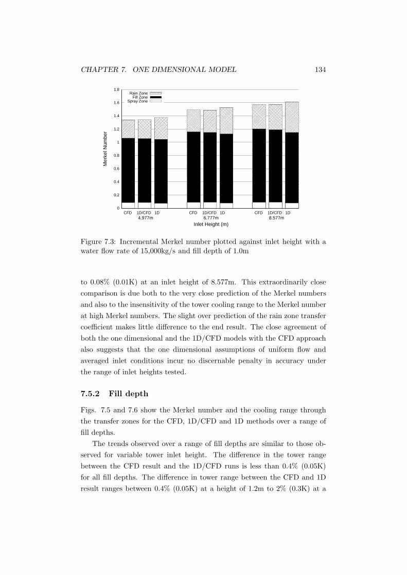
CHAPTER 7. ONE DIMENSIONAL MODEL 134
0
0.2
0.4
0.6
0.8
1
1.2
1.4
1.6
1.8
Mer
kel N
umbe
r
Inlet Height (m)
CFD 1D/CFD 1D CFD 1D/CFD 1DCFD 1D/CFD 1D4.977m 6.777m 8.577m
Rain ZoneFill Zone
Spray Zone
Figure 7.3: Incremental Merkel number plotted against inlet height with awater flow rate of 15,000kg/s and fill depth of 1.0m
to 0.08% (0.01K) at an inlet height of 8.577m. This extraordinarily close
comparison is due both to the very close prediction of the Merkel numbers
and also to the insensitivity of the tower cooling range to the Merkel number
at high Merkel numbers. The slight over prediction of the rain zone transfer
coefficient makes little difference to the end result. The close agreement of
both the one dimensional and the 1D/CFD models with the CFD approach
also suggests that the one dimensional assumptions of uniform flow and
averaged inlet conditions incur no discernable penalty in accuracy under
the range of inlet heights tested.
7.5.2 Fill depth
Figs. 7.5 and 7.6 show the Merkel number and the cooling range through
the transfer zones for the CFD, 1D/CFD and 1D methods over a range of
fill depths.
The trends observed over a range of fill depths are similar to those ob-
served for variable tower inlet height. The difference in the tower range
between the CFD result and the 1D/CFD runs is less than 0.4% (0.05K)
for all fill depths. The difference in tower range between the CFD and 1D
result ranges between 0.4% (0.05K) at a height of 1.2m to 2% (0.3K) at a

CHAPTER 7. ONE DIMENSIONAL MODEL 135
0
2
4
6
8
10
12
14
16
Incr
emen
tal T
ower
Coo
ling
Ran
ge (
K)
Inlet Height (m)
CFD 1D/CFD 1D CFD 1D/CFD 1DCFD 1D/CFD 1D4.977m 6.777m 8.577m
Rain ZoneFill Zone
Spray Zone
Figure 7.4: Incremental cooling range plotted against inlet height with awater flow rate of 15,000kg/s and fill depth of 1.0m
height of 0.6m. The difference between the CFD predicted air flow and the
1D models predicted air flow ranges between 1 and 2%.
The predicted rain zone Merkel number is about 23% larger in the one
dimensional method than the CFD results which explains the slightly larger
tower range predicted by the 1D method.
These results appear consistent across all three fill depths tested with the
relative difference between the CFD results and the standard 1D methods
perhaps slightly better at the larger fill depths.
7.5.3 Water flow rate
Figs. 7.7 and 7.8 show the Merkel number and the cooling range through
the transfer zones for the CFD, 1D/CFD and 1D methods over a range of
water flow rates.
The correlation for the loss coefficient for the tower inlet is only valid for
water mass fluxes between 1 − 3kg/s/m2 [3], hence is not valid for the flow
rates of 22,500kg/s and 30,000kg/s. In addition, the rain zone loss coefficient
and transfer coefficient are not valid over this range. In these cases the one
dimensional method has not been solved, only the 1D/CFD method and the
CFD method.
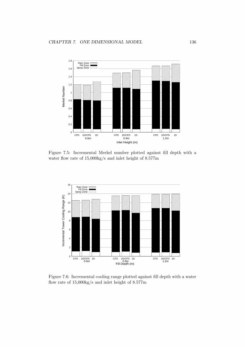
CHAPTER 7. ONE DIMENSIONAL MODEL 136
0
0.2
0.4
0.6
0.8
1
1.2
1.4
1.6
1.8
Mer
kel N
umbe
r
Inlet Height (m)
CFD 1D/CFD 1D CFD 1D/CFD 1DCFD 1D/CFD 1D0.6m 0.9m 1.2m
Rain ZoneFill Zone
Spray Zone
Figure 7.5: Incremental Merkel number plotted against fill depth with awater flow rate of 15,000kg/s and inlet height of 8.577m
0
2
4
6
8
10
12
14
16
Incr
emen
tal T
ower
Coo
ling
Ran
ge (
K)
Fill Depth (m)
CFD 1D/CFD 1D CFD 1D/CFD 1DCFD 1D/CFD 1D0.6m 0.9m 1.2m
Rain ZoneFill Zone
Spray Zone
Figure 7.6: Incremental cooling range plotted against fill depth with a waterflow rate of 15,000kg/s and inlet height of 8.577m
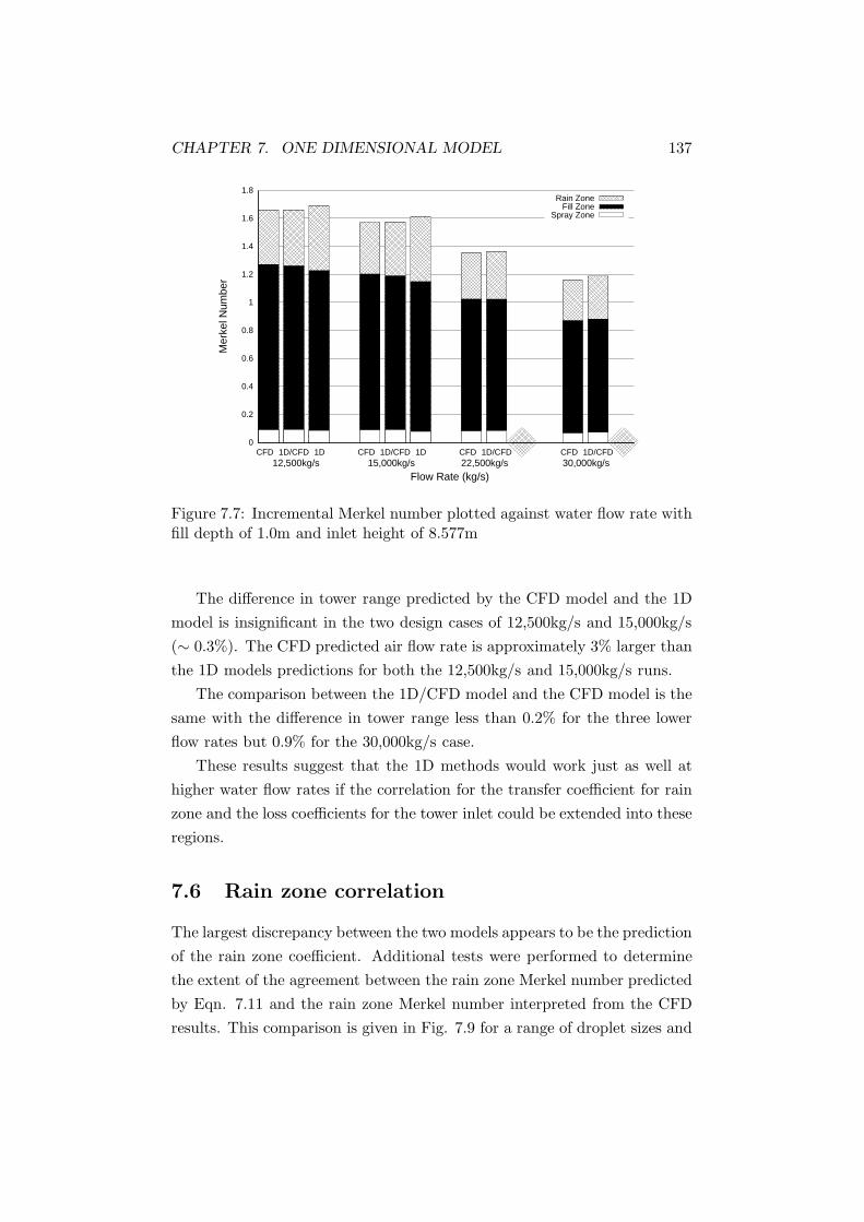
CHAPTER 7. ONE DIMENSIONAL MODEL 137
0
0.2
0.4
0.6
0.8
1
1.2
1.4
1.6
1.8
Mer
kel N
umbe
r
Flow Rate (kg/s)
CFD 1D/CFD 1D CFD 1D/CFD 1D CFD 1D/CFD CFD 1D/CFD12,500kg/s 15,000kg/s 22,500kg/s 30,000kg/s
Rain ZoneFill Zone
Spray Zone
Figure 7.7: Incremental Merkel number plotted against water flow rate withfill depth of 1.0m and inlet height of 8.577m
The difference in tower range predicted by the CFD model and the 1D
model is insignificant in the two design cases of 12,500kg/s and 15,000kg/s
(∼ 0.3%). The CFD predicted air flow rate is approximately 3% larger than
the 1D models predictions for both the 12,500kg/s and 15,000kg/s runs.
The comparison between the 1D/CFD model and the CFD model is the
same with the difference in tower range less than 0.2% for the three lower
flow rates but 0.9% for the 30,000kg/s case.
These results suggest that the 1D methods would work just as well at
higher water flow rates if the correlation for the transfer coefficient for rain
zone and the loss coefficients for the tower inlet could be extended into these
regions.
7.6 Rain zone correlation
The largest discrepancy between the two models appears to be the prediction
of the rain zone coefficient. Additional tests were performed to determine
the extent of the agreement between the rain zone Merkel number predicted
by Eqn. 7.11 and the rain zone Merkel number interpreted from the CFD
results. This comparison is given in Fig. 7.9 for a range of droplet sizes and

CHAPTER 7. ONE DIMENSIONAL MODEL 138
0
2
4
6
8
10
12
14
16
Incr
emen
tal T
ower
Coo
ling
Ran
ge (
K)
Flow Rate (kg/s)
CFD 1D/CFD 1D CFD 1D/CFD 1D CFD 1D/CFD CFD 1D/CFD12,500kg/s 15,000kg/s 22,500kg/s 30,000kg/s
Rain ZoneFill Zone
Spray Zone
Figure 7.8: Incremental cooling range plotted against water flow rate withfill depth of 1.0m and inlet height of 8.577m
inlet heights.
The effect of rain zone droplet size distribution has been examined by
plotting CFD results with uniform droplet size distribution in the rain zone
and with the droplet size distribution given in Table 5.3. The fluid flow
properties, the air-vapour velocity and other constants in Eqn. 7.11, have
been taken from the CFD model results with the droplet distribution at
each inlet height. The differences in these properties between the uniform
and non-uniform distributions are very small however and have no effect on
the comparisons in the plot.
The plot shows the agreement between Eqn. 7.11 and the CFD results
for uniform droplet diameters is very good at large droplet diameters, but
gets worse with decreasing droplet diameter. Both the CFD model and the
derivation of Eqn. 7.11 rely on general droplet empirical heat and mass
transfer correlations. The CFD model is a more detailed representation of
air flow and droplet trajectory integration however, which may be important.
In the derivation of Eqn 7.11, the droplet flow is assumed to have no effect
on the air flow. Also in the CFD model, the calculations are not performed
in isolation, but as part of the tower, so the air temperature/humidity and
water temperature vary across the tower. Neither the CFD model or Eqn.

CHAPTER 7. ONE DIMENSIONAL MODEL 139
3 4 5 6 7 8
x 10−3
0
0.2
0.4
0.6
Mer
kel N
umbe
r
Droplet Diameter (m)
CFD distibution H = 8.577CFD distibution H = 6.777CFD distibution H = 4.977CFD h = 8.577h = 4.977h = 6.777h = 8.577
Figure 7.9: Merkel number interpreted from CFD results compared withcorrelation in Kroger [1]
7.11 take into account droplet amalgamation or the effect of turbulence on
droplet heat and mass transfer. Detailed experimental results are needed to
verify the above predictions.
The comparison is much worse with a non-uniform droplet distribution.
At all inlet heights, Eqn. 7.11 overpredicts the Merkel number compared to
the CFD result with non-uniform droplet diameter. The Merkel number for
the non-uniform droplet diameter is about 10% less than that for the uniform
distribution at the same Sauter mean diameter. This follows the conclusions
in section 5.11 and section 6.2.6, that the behaviour of a non-uniform droplet
distribution is quite different from that of a uniform distribution and that
this is not entirely captured by the Sauter mean diameter. The source of
the disagreement in the rain zone transfer coefficient in the previous sections
is very likely due to additional effects related to the non-uniform droplet
distribution, which is not captured in Eqn. 7.11.

CHAPTER 7. ONE DIMENSIONAL MODEL 140
1 1.526
27
28
29
30
31
32
33
34
Wat
er O
utle
t Tem
pera
ture
( o C
)
Merkel Number
ima
= 50,000ima
= 70,000ima
= 90000
Figure 7.10: Water outlet temperature with Merkel number
7.7 Sensitivity of performance to Merkel number
In all the cases presented in this chapter, the predicted water outlet tem-
peratures for the CFD model and the one dimensional model are very close,
in spite of quite noticeable differences in the Merkel numbers. This is be-
cause heat transfer becomes less sensitive to Merkel number at higher Merkel
numbers. This is shown in Fig. 7.10 as a function of air inlet enthalpy.
ima = 50, 000J/Kg corresponds to approximately standard reference inlet
conditions and ima = 90, 000J/Kg, the air condition at the centre of the
tower (under reference conditions) where it has been significantly heated.
Increasing the Merkel number from 1.6 to 1.7 results in an increase in water
outlet temperature of about only 0.1K under standard tower design condi-
tions.
7.8 Poppe model comparison
Kloppers [3] compared the transfer characteristics for a particular fill found
using the Poppe approach and the Merkel approach. The author found that
across a broad range of ambient temperatures and humidities, the transfer
coefficient found using the Poppe approach was 7% larger than the one found

CHAPTER 7. ONE DIMENSIONAL MODEL 141
using the Merkel approach. Thus the author concluded that the transfer
correlations derived in Merkel format can be converted by increaseing them
by 7%. This rule of thumb has been used here to convert the rain zone
and spray zone transfer coefficient correlations in Eqn. 7.13 and Eqn. 7.11
into Poppe format. This has then been used to peform the comparison in
this chapter again using the Poppe model instead of the Merkel model. The
results of this comparison are very similar to those above so have not been
presented here.
7.9 Conclusion
A comparison has been made between a one dimensional NDWCT model
with Merkel heat transfer routine and a two dimensional CFD model. The
difference between the predictions of tower cooling range is very low, gener-
ally around 1-2%. This small difference appears to be due to a combination
of a slight difference in the prediction of the air flow rate and the corre-
lations for the transfer coefficient for the rain zone. The prediction of the
fill Merkel number by the one-dimensional method, appears to be slightly
conservative in all cases, but the difference is very small. In all cases the
rain zone Merkel number predicted by Eqn. 7.11 was greater than the CFD
result. The difference in the prediction of the tower draft is generally less
than 3%.
Additional tests were performed to determine the effect of the assump-
tions in the one dimensional model of uniform air flow through the fill and
averaged fill inlet air conditions. To make the test fair, the CFD results
were compared against the predictions of a one dimensional model in which
the air flow rate, and the rain and spray zone Merkel numbers were taken
from the CFD model. The difference between the tower range predicted by
the two models has been shown to be less than 0.4% in most cases. This
extraordinarily close comparison supports the one dimensional assumptions.
Furthermore, under the range of parameters tested here the difference be-
tween the CFD models predictions and those of the one dimensional models
remained fairly constant, suggesting that there is no particular area where
the flow becomes so skewed or non-uniform that the one dimensional model
predictions begin to fail. These results indicate that while there is significant
non-uniformity of heat transfer across the tower, the overall heat transfer is

CHAPTER 7. ONE DIMENSIONAL MODEL 142
essentially one-dimensional with respect to the variables tested.
For large rain zone droplet diameters, close agreement was found be-
tween the CFD model predictions of rain zone Merkel number and the semi-
empirical correlation in Eqn. 7.11. At small droplet diameters the agreement
is not as good and may indicate limitations of this correlation. Additionally,
the results with a non-uniform droplet distribution were found to compare
more poorly than those for the uniform distribution.

Chapter 8
Extendend One-Dimensional
Modelling and Optimisation
8.1 Introduction
The one dimensional model described in Chapter 7 is the type of model used
in NDWCT design and optimisation studies. The one dimensional nature of
the method places limitations on the range of design configurations that can
be considered. The fill depth and the water flow rate must be uniform across
the tower as non-uniform fill and water distributions cannot be resolved by
the one dimensional models. There is suggestion in literature that this is not
an optimal configuration and that other layouts should be considered [1].
In some instances designers have even opted to make ad-hoc attempts at
guessing the optimal fill layout and water distribution [1].
The purpose of this chapter is to attempt to quantify the improvement
in performance that can be achieved by using non-uniform fill and water
distribution. To this end an optimisation study has been undertaken using
the CFD model described in Chapter 5 and a new one dimensional model
which is described in this chapter. This new model is a simple extension
of the one dimensional design method described in Chapter 7. The exten-
sions allow two dimensional fill and water distribution configurations to be
simulated.
143
CHAPTER 8. TWO DIMENSIONAL OPTIMISATION 144
8.2 Previous work
A number of cooling tower economic and thermal optimisation studies have
appeared in literature, covering a range of cooling tower configurations. Lu
et al. [109] developed a model of a HVAC cooling system with a forced flow
cooling tower with variable fan speed and water load. They use a modified
genetic algorithm to find the optimal set points for fan and pump load to
minimise overall condenser loop power consumption. The authors found
that varying the fan speed and pump flow rate to match ambient conditions
saved as much as 50% at part load and 10% at full load in comparison to
the traditional system configurations. The savings were mostly due to the
savings in fan and pump power but also due to an increase in cooling tower
efficiency with a higher water supply temperature increasing the difference
between that and the ambient temperature enabling it to reject more heat.
Kintner-Meyer and Emery [110] conducted an optimisation study for a
chiller cooling system incorporating a forced draft cooling tower. The author
examined the relative contribution of the operating and capital costs under
a range of air and water temperatures. The author found that when consid-
ering the cooling tower on its own, there was significant room for reduction
in total cost but that when the entire system was considered including the
chiller plant, the cooling tower was a less significant part of the total cost.
The authors also noted that their study was only at full load and that at
part load the trade off between operating costs and capital costs is more
important.
Kloppers and Kroger [106] used their one-dimensional model of NDWCT
to find the optimal geometric dimensions of the tower that minimised its
cost over its entire operational life. The study considered a tower of similar
dimensions to the one in this study. The authors found the pumping cost
to be a significant factor in the model design. The optimal design reduced
the water distribution height and hence the tower inlet height significantly,
down to 4.9m. The authors noted that such a design also reduces the tower’s
susceptibility to cross-wind related performance penalties. Other changes
in the optimal model included a small decrease in tower diameter, small
decrease in tower height and a large increase in fill depth. The changes
reduced the cost of the tower by 18.7% over its useful life. This is the most
complete NDWCT optimisation study so far to appear in the literature.

CHAPTER 8. TWO DIMENSIONAL OPTIMISATION 145
Conradie et al. [19] performed a similar study to determine the optimal
design parameters for a dry cooling tower. They examined in detail the
costs of the entire plant and were able to reduce the cost of the cooling
system through modification of the tower’s geometry and heat exchanger
design.
Radosavljevic’s [5] study into NDWCTs has aspects that are similar to
the study considered here. The author used a two-dimensional axisymmetric
numerical model to run a parametric study to determine the effect of chang-
ing the fill shape and water distribution. The author found that removing a
small amount of fill from the centre of the tower, while maintaining the same
overall fill volume, improved the tower performance, but by only 0.03K. A
very limited range of fill shapes were tested with no optimisation study.
In some instances designers have opted to counter the radial heat and
mass transfer profiles and improve tower performance by having a fill of
variable depth across the tower [1]. There has been no formal investigation
to determine the optimal fill layout and water distribution across the tower
appearing in the literature to date.
Here an attempt is made to quantify the improvement possible by vary-
ing both the water flow rate and fill depth across the tower. An evolutionary
optimisation routine has been implemented here. A number of recent pub-
lications have employed such techniques for shape optimisation [111–114].
Such algorithms operate by evaluating a large number of points in the so-
lution space, typically above 2000. It is therefore essential that the model
or fitness function allows rapid evaluation of these points. While a two di-
mensional CFD model has a high resolution it takes orders of magnitude
longer to solve than a simple one dimensional model so is unsuited for use
in an optimisation study. Here instead, an extended one dimensional model
is developed as an attempt to retain partial two dimensional resolution in
the fill region, without the time penalty of a full Navier Stokes solver. This
extended model has been termed a ’1D-zonal’ model and is simply a one-
dimensional model which has semi-two dimensional capability in the fill and
spray zone regions.
This chapter is laid out as follows. In sections 8.3 and 8.4, an extended
one dimensional model is presented. The optimisation problem and the
evolutionary optimisation procedure are described in section 8.5 and section
8.6. The results of the optimisation together with a comparison between the

CHAPTER 8. TWO DIMENSIONAL OPTIMISATION 146
6
66 6 6 6(1) (2) (3) (4)
Figure 8.1: Schematic representation of 1D zonal model air flow path in heattransfer region with four zones; (1) (Lfi,1 and Gw,1), (2) (Lfi,2 and Gw,2),(3) (Lfi,3 and Gw,3), (4) (Lfi,4 and Gw,4)
CFD model solution and the extended 1D model solution for the optimal
set of parameters is given in section 8.7.
8.3 Extended one-dimensional-zonal model
The 1D-zonal model is essentially the same as the one dimensional model
described in Chapter 7. The difference is that the fill itself is divided into a
number of zones (four in this study) in parallel, each with independent fill
depth and water flow rate (Fig. 8.1). The air flow rate and heat transfer for
each zone are calculated separately. The enthalpy of the air/water vapour
mixture at the inlet of each fill zone (ima,fi,i), is determined by forcing the
calculated average enthalpy before the fill to an empirical profile. This profile
has been derived from results from the two dimensional CFD presented in
Chapter 5. In this way the two dimensional behaviour of the 1D-zonal model
is entirely represented through the specification of the air enthalpy profile
across the tower.
In order to examine the generality of such an approach, the sensitivity
of the air/water vapour enthalpy profile shape, to a range of design and
operating parameters has been tested. These results are plotted in Fig. 8.2
and Fig. 8.3. These plots can be viewed as an axisymmetric section with
the centre of the tower at a radius of 0m and the tower inlet located at a
radius of 46.8m (see Fig. 5.1). The heat and mass transfer regions extend

CHAPTER 8. TWO DIMENSIONAL OPTIMISATION 147
from the tower inlet to the causeway at a radius of 1.4m. Unless otherwise
stated the fill depth is 1.0m, the water flow rate 15,000kg/s, the droplets
in the rain zone follow the distribution given in Table 5.3, the tower inlet
height is 8.577m and the ambient air is at 295K and 55% relative humidity.
The air/water vapour mixture enthalpy at the fill inlet has been calculated
using Eqn. 8.1:
ima,fi,i = CpaTa,fi,i + ωfi,i(ifgwo + CpvTa,fi,i), (8.1)
where ifgwo is the enthalpy of vaporisation of water at zero degrees Celsius
and is approximately equal to 2501.6 kJ/kg.
Following the discussion in Chapter 6, the results in Fig. 8.2 and Fig.
8.3 show the ima,fi,i profile is strongly related to the heat and mass transfer
in the rain zone. At low fill depths, the water temperature entering the rain
zone is higher, increasing the driving force for heat and mass transfer in the
rain zone and the overall ima,fi,i gradient across the tower (Fig. 8.2 (c)).
With small rain zone water droplet diameters, the heat transfer area is higher
and therefore the heat and mass transfer increases as shown in Fig. 8.3 (a).
The relative ratio of the air and water flow rate is also important. Increasing
the water flow rate increases the thermal mass of water, increasing the overall
heat transfer (Fig. 8.3 (b)). Decreasing the rain zone height has little effect
on the enthalpy gradient (Fig. 8.2 (b)). The ambient temperature and
humidity have the effect of vertically shifting the ima,fi,i profile as illustrated
in Fig. 8.2 (a).
Overall these results show the shape of the profile or the gradient of the
air enthalpy from the tower inlet to the centre of the tower, is relatively
insensitive to small changes in water flow rate and fill depth. This indicates
that the approach taken here of specifying a fixed profile is a reasonable
approximation. Here we are interested in varying the fill depth and water
flow rate by relatively small amounts so the air enthalpy profile is assumed
to deviate only slightly from the standard case. The ima,fi,i profile under
the standard reference conditions (see Table 5.1) is fitted with Eqn. 8.2,
i′ma,fi,i = −0.432x3 + 37.5x2 − 1870x + 98800, (8.2)
where x is the radial distance from the centre of the tower.

CHAPTER 8. TWO DIMENSIONAL OPTIMISATION 148
20000
30000
40000
50000
60000
70000
80000
90000
100000
110000
0 5 10 15 20 25 30 35 40 45 50
i ma
(J/k
g)
Radius (m)
Ta = 285 RH40%Ta = 300 RH40%
Ta = 285 RH61.5%Ta = 300 RH61.5%
(a)
45000
50000
55000
60000
65000
70000
75000
80000
85000
90000
95000
100000
0 5 10 15 20 25 30 35 40 45 50
i ma
(J/k
g)
Radius (m)
inlet height 4.977minlet height 6.777minlet height 8.577m
(b)
40000
50000
60000
70000
80000
90000
100000
0 5 10 15 20 25 30 35 40 45 50
i ma
(J/k
g)
Radius (m)
fill depth 0.6mfill depth 0.9mfill depth 1.2m
(c)
Figure 8.2: Annular profile of air/water vapour enthalpy at the entrance tothe fill, with variable ambient conditions (a), variable tower inlet height (b)and variable fill depth (c)

CHAPTER 8. TWO DIMENSIONAL OPTIMISATION 149
40000
50000
60000
70000
80000
90000
100000
0 5 10 15 20 25 30 35 40 45 50
i ma
(J/k
g)
Radius (m)
droplet diameter = 3.31mmdroplet diameter = 5.31mmdroplet diameter = 7.31mm
(a)
40000
50000
60000
70000
80000
90000
100000
110000
120000
130000
140000
0 5 10 15 20 25 30 35 40 45 50
i ma
(J/k
g)
Radius (m)
12500kg/s15000kg/s22500kg/s30000kg/s
(b)
45000
50000
55000
60000
65000
70000
75000
80000
85000
90000
95000
0 5 10 15 20 25 30 35 40 45 50
i ma
(J/k
g)
Radius (m)
CFD (profile)CFD (uniform)
zonal 1D (profile)
(c)
Figure 8.3: Annular profile of air/water vapour enthalpy at the entrance tothe fill, with variable rain zone droplet size (a), variable water flow rate (b)and under reference conditions with the fill depth and water distributionfound in run one (Table 8.2) (c)

CHAPTER 8. TWO DIMENSIONAL OPTIMISATION 150
8.4 Model procedure
The 1D-zonal model solution procedure is described in Fig. 8.4. It is very
similar to one dimensional model in Chapter 7, where the Merkel model
is used for the heat and mass transfer and the simple draft equation is
solved for the air flow (Eqn. 7.1). The additional modelling assumptions
are summarised as follows:
1. The pressure drop is uniform across all fill sections.
2. The airflow through the fill is assumed to remain fairly uniform, such
that the rain zone transfer coefficient (Eqn. 7.11) and loss coefficient
(Eqn. 7.12) and the loss coefficients for the tower inlet (Eqn. 7.15)
taken from Kroger [1] can be applied.
3. The enthalpy profile specified at the fill inlet is assumed to remain
constant despite changes to fill shape and water distribution.
4. The loss coefficient for the rain zone affects all the fill sections equally.
The heat and mass transfer process is split between the rain zone and
the fill zones. The average air/water vapour enthalpy leaving the rain zone
(ima,rz,o) is found by solving the Merkel model for the rain zone (Table 2.3),
between the average water temperature leaving the fill (Tw,rz,i) and the tower
water outlet temperature (Tw,rz,o). The average air/water vapour enthalpy
leaving the rain zone, ima,rz,o, and entering each fill zone, j, is determined
by Eqn. 8.3,
ijma,fi,i = i′jma,fi,i
ima,rz,oma,total
∑kj=1
[i′jma,fi,i · m
ja
] , (8.3)
where mja is the dry air mass flow rate in each fill zone, ma,total is the
total dry air mass flow rate in the tower and i′jma,fi,i is the average enthalpy
entering each fill zone under reference conditions, calculated using Eqn. 8.2.
In this way the average enthalpy entering the fill is still ima,rz,o, but the
profile now has the same shape as Eqn. 8.2. The entire process (given in
Fig. 8.4) is very iterative, with the guessed and calculated values for ima,rz,o,
Tw,o and ma required to be within the tolerances specified, δma , δMe, δima,rz .
In this study, δMe = 5 × 10⁻⁵, δma = 1 × 10⁻¹kg/s, δima,rz = 10J/Kg and
Crelax = 0.8.

CHAPTER 8. TWO DIMENSIONAL OPTIMISATION 151
1 Initialisation of variables: specify mjw, Lj
fi, Ta,i Tw,i,δma , δMe, δima,rz
2 Guess T jw,fi,o, ima,rz,o and Ta,o
3 Estimate ma and mja to find Ktot, Kj
fi
4 Solve tower draft equation (Eqn. 7.1) using the guessed Ta,o,to find ma (see Appendix C)
5 c = 1;6 While : δc
ma> δma
7 c = c + 1; n = 08 While : δn
ima,rz> δima,rz
9 n = n + 110 inma,rz,o = in−1
ma,rz,o
11 For j = 1,2...k
12 Calculate ijma,fi,i using Eqn. 8.3 and inma,rz,o
13 Calculate Mejfi and Mesp,i using Eqn. 7.5 and Eqn. 7.13
14 Solve the Merkel equations for fill zone j, using the
procedure in Table 2.3 (b),to find T jw,fi,o
15 Find the average water temperature entering the rain zone,
Tw,rz,i =∑k
j=1 T jw,fi,om
jw/mw
16 Calculate Merz using Eqn. 7.1117 Solve the Merkel equations, for the rain zone region, using
the procedure in Table 2.3 (b), to find Tw,rz,o and inma,rz,o
18 δnima,rz
= inma,rz,o − in−1ma,rz,o
19 Calculate Ta,fi,o from bulk average ima,fi,o, using Eqn. B.1720 m = 0 , m′m
a = mca
21 While δ′mma> δma
22 m = m + 123 m′m
a = m′m−1a + Crelax(m
′ma − m′m−1
a )
24 Calculate loss coefficient for each fill zone Kjfi,z, using Eqn. 7.9
25 Calculate the loss coefficient for all components in thetower except the fill: Knfi (see Appendix C)
26 Calculate pressure head available ∆Ptot = (ρ∞ − ρa,o)gHtower
i.e. (Eqn. 7.1)27 Calculate pressure drop across components except for the fill
∆Pother = KnfiρV 2
2 (see Appendix C)28 Calculate pressure drop across the fill ∆Pfill = ∆Ptot − ∆Pnfi
29 Calculate air flow rate mja across the fill zones assuming
equal pressure drop ( ∆Pfill) across each zone
30 Sum to find total air flow in the tower m′m+1a =
∑kj=1 mj
a
31 δ′mma= m′m+1
a − m′ma
32 mc+1a = m′m+1
a
33 δcma
= mc+1a − cn
a
34 END
Figure 8.4: 1D-zonal model solver procedure
CHAPTER 8. TWO DIMENSIONAL OPTIMISATION 152
8.5 Problem description
Here we have attempted to optimise a standard NDWCT fill and water
distribution across the tower such that the fill and water volume remain
constant. The 1D-zonal model has been divided into four sections with the
fill depth and water distribution uniform across each of the sections. The
objective function to be maximised is the tower range (Trange = Twi −Two).
The search space is bounded by the following constraints:
The water flow rate for Gw,1 to Gw,3 can vary between 2.0 < Gw < 2.3.
The fill depth Lfi,1 to Lfi,3 can range between 0.6 < Lfi < 1.2. The
constraint for constant total fill volume is enforced through Lfi,4 such that
Lfi,4 =
(Vfill,tot − [
∑3n=1 Lfi,n · Af,n]
)/Af,4, where Vfill,tot is the total fill
volume such that the average fill depth is 1.0m. The total water flow rate
Gw,tot (15,000kg/s) is enforced through Gw,4 such that Gw,4 =
(15, 000 −
[∑3
n=1 Gw,n · Af,n]
)/Af,4.
8.6 Evolutionary algorithm procedure
The optimisation procedure implemented here is an evolutionary algorithm,
similar to that described in Michalewicz [115]. These routines have been
shown to be robust and reliable in conditions where traditional methods
can fail to find a global optimum [115, 116]. They have been widely studied
and implemented in a variety of difficult engineering problems [111–114].
The basic operation of this algorithm is presented here for completeness.
An ’individual’ is a collated string of system variables. Each variable is
represented using floating point numbers.
The algorithm proceeds as depicted in Fig. 8.5, where an initial pop-
ulation undergoes mutation, cross-over and selection operations until the
termination conditions are reached. An elitist strategy is implemented here
where the best individual from each generation is retained and is used to
replace the least fit individual. This allows high mutation and crossover
rates to be employed without fear of losing the good candidates [116]. The
operator probabilities and other algorithm constants are contained in Table
8.1.

CHAPTER 8. TWO DIMENSIONAL OPTIMISATION 153
1) Begin2) Initialise population3) Evaluate objective function4) Store best individual5) Selection: generate a
new mating population withtournament selection
6) Apply cross-over andmutation operators
7) Store current population8) If generation < max
generations goto (3)
9) End
Figure 8.5: Schematic representation of the evolutionary algorithm proce-dure
8.6.1 Selection operators
Here the tournament selection method is implemented. These selection pro-
cedures do not use the fitness values directly in selection, only the relative
rank of the individuals [115]. In this method, individuals compete against
each other in many small ’tournaments’, where the most fit member is se-
lected for the new population. The method proceeds as follows: k individuals
are randomly chosen from the old population. The most fit individual from
this subset is selected for the next generation. This procedure is repeated
until the new population is filled. The larger the value of k, the higher the
selection pressure.
8.6.2 Mutation operators
Three floating point mutation operators were employed for the optimi-
sation study. These are taken from Michalewicz [115]. In all cases, a
single candidate X ′ = (x1, ..., x′
j , ..., xn) is created from a single parent
X = (x1, ..., xj , ..., xn) by randomly selecting and replacing the element xj
of a parent X with x′
j where, j ∈ (1, ..., n) and x′
j lies within the feasible
range 〈Lj , Uj〉. The method of generating x′
j is unique to each mutation
operator.

CHAPTER 8. TWO DIMENSIONAL OPTIMISATION 154
Table 8.1: Evolutionary algorithm operator probabilities and parametersOperator Value
Probability of non-uniform mutation 0.20Shape parameter (b) 3.0
Probability of uniform mutation 0.05Probability of heuristic crossover 0.05
Probability of arithmetic crossover 0.05Probability of simple crossover 0.05
Population 30Max no. of generations 200Tournament size (k) 2
Heuristic cross over attempts (w) 5
Uniform mutation
This operator sets x′
j equal to a random number with a uniform probability
distribution in the feasible range 〈Lj , Uj〉. The operator is important early
in the search as it covers the search space with uniform probability.
Non-uniform mutation
This operator is a function of generation, where the allowable mutation gets
smaller with each succeeding generation. The operator randomly determines
if the selected variable, x′
j, should be mutated in the direction of its upper or
lower boundary such that x′
j = xj+(Uj−xj)∗f(t) or x′
j = xj−(xj−Lj)∗f(t),
if a uniform random number, r1, is < 0.5 or ≥ 0.5 respectively. The shape
function is f(t) = r2 · (1 − tTmax
)b, where Tmax is the maximum number of
generations, t is the current generation, b is the shape parameter (=3) and
r1 and r2 are random numbers between 0 and 1.
8.6.3 Crossover operators
Three crossover operators are employed in this study. These are taken from
[115].
Simple crossover
Two parent individuals X = (x1, ..., xn) and Y = (y1, ..., yn), are cut at
the jth position and rejoined here to create two new individuals X ′ =

CHAPTER 8. TWO DIMENSIONAL OPTIMISATION 155
(x1, ..., xj , yj+1..., yn) and Y ′ = (y1, ..., yj , xj+1, ..., xn).
Heuristic crossover
This operator uses fitness information to create a single new individual X ′
from two parents X and Y . The new individual is X ′ = r · (X − Y ) + X,
where X has a higher fitness than Y (for maximisation problems) and r
is a random number between 0 and 1. This may fall outside the feasible
solution space so if after w attempts no feasible solution is produced, the
operation is terminated and no new offspring is created. The operators
unique contribution is that it uses fitness information to select a promising
search direction.
Arithmetic crossover
This operator produces two new individuals X ′ and Y ′ from two parents X
and Y with X ′ = r · X + (1 − r)Y and Y ′ = r · Y + (1 − r)X, where r is a
random number between 0 and 1. This allows the linear combination of two
parents with a random amount of mixing.
8.7 Results and discussion
The optimisation routine has been run four times as it is a stochastic process
with results slightly different each time (Table 8.2). The centre variables
Lfi,1 and Gw,1 affect the solution very weakly so they have some variation
in the final solution. The axisymmetric geometry means the fill volume per
unit radius increases with radius, so changes in the tower centre have less of
an effect on the overall tower performance.
The difference in water outlet temperatures predicted by the CFD model
and the 1D zonal method is approximately 0.04K. The improvement of the
fill depth and water distribution profile can be compared against a uniform
fill and water distribution in row 5 of Table 8.2. The improvements predicted
by the two models are identical in all but one case, supporting the models
equivalence.
The air enthalpy at the entrance to the fill is slightly over-predicted by
the 1D-zonal model (Fig. 8.3 (c)) compared to the CFD model. This follows
the conclusions presented in Chapter 7, that the rain zone transfer coefficient
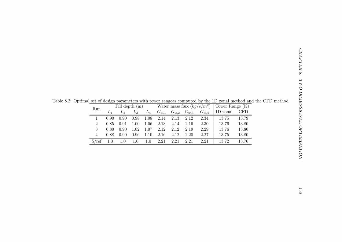
CH
AP
TE
R8.
TW
OD
IME
NSIO
NA
LO
PT
IMIS
AT
ION
156
Table 8.2: Optimal set of design parameters with tower rangeas computed by the 1D zonal method and the CFD methodFill depth (m) Water mass flux (kg/s/m2) Tower Range (K)
RunL1 L2 L3 L4 Gw,1 Gw,2 Gw,3 Gw,4 1D-zonal CFD
1 0.90 0.90 0.98 1.08 2.14 2.13 2.12 2.34 13.75 13.792 0.85 0.91 1.00 1.06 2.13 2.14 2.16 2.30 13.76 13.803 0.80 0.90 1.02 1.07 2.12 2.12 2.19 2.29 13.76 13.804 0.88 0.90 0.96 1.10 2.16 2.12 2.20 2.27 13.75 13.80
5/ref 1.0 1.0 1.0 1.0 2.21 2.21 2.21 2.21 13.72 13.76

CHAPTER 8. TWO DIMENSIONAL OPTIMISATION 157
given in [1] is over-predicted for non-uniform droplet size distributions. The
air enthalpy profile predicted by the CFD model under the uniform case is
quite close to the CFD results with the fill and water distribution from run
one. This supports the original assumptions that for small changes in fill
depth and water flow rate the ima profile changes very little.
A comparison of the CFD and the 1D zonal results for the parameters
in run one show very good agreement (Fig. 8.6 - Fig. 8.7 and Table 8.2).
The 1D-zonal model predicts air flow within 5% of the CFD value (Fig. 8.6
(a)). The water temperature below the fill follows the same trend as the
CFD method in each of the four zones (Fig. 8.6 (b)). Overall the 1D-zonal
model predicts the heat transfer and airflow distribution well.
On the same plots, a comparison is made between the CFD results of a
uniform fill and water distribution profile. The lower fill depth in the tower
centre has the effect of increasing the air flow there and reducing it in the
outer region. The actual overall heat transfer to the air from the tower inlet
to the fill outlet changes very little, although the air temperature at the fill
outlet is reduced slightly with the shallower fill and higher air flow here.
The overall improvement in performance with the optimal profile has
been shown to be very marginal, with an increase in water range of only
0.04K. With a fixed fill volume, a big decrease in fill depth at the tower
centre only allows a relatively small increase in fill depth in the tower’s outer
regions. Additionally, this study shows that Lowe and Christie [7] were not
entirely correct that the air has ”already been heated nearly to capacity” in
the centre of the tower. Figs. 6.1 - 6.18 show that except at very high water
flow rates, the cooling in the centre of the tower is still significant. Entirely
sacrificing this cooling for the outer regions is not optimal.
As discussed previously, since the non-uniformity is specified through
the ima profile, we can draw some conclusions as to the generality of the
result. The ima profiles are independent of tower inlet height, fill depth
and ambient air temperature and humidity (see Fig. 8.2 and 8.3) so the
results here should apply over these conditions. The optimisation is likely
to be more effective at very high water flow rates as indicated by the large
variation in ima across the tower in Fig. 8.3 for mw = 30, 000 kg/s. For the
range of variables tested here however, the results show that two-dimensional
optimisation is unnecessary and a uniform fill and water distribution profile
is adequate.
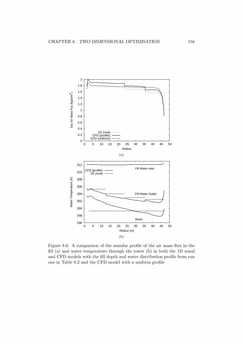
CHAPTER 8. TWO DIMENSIONAL OPTIMISATION 158
0
0.2
0.4
0.6
0.8
1
1.2
1.4
1.6
1.8
2
0 5 10 15 20 25 30 35 40 45 50
Dry
Air
Mas
s F
ux (
kg/s
/m2 )
Radius
1D zonalCFD (profile)
CFD (uniform)
(a)
296
298
300
302
304
306
308
310
312
0 5 10 15 20 25 30 35 40 45 50
Wat
er T
empe
ratu
re (
K)
Radius (m)
Fill Water Inlet
Fill Water Outlet
Basin
CFD (profile)1D zonal
(b)
Figure 8.6: A comparison of the annular profile of the air mass flux in thefill (a) and water temperature through the tower (b) in both the 1D zonaland CFD models with the fill depth and water distribution profile from runone in Table 8.2 and the CFD model with a uniform profile

CHAPTER 8. TWO DIMENSIONAL OPTIMISATION 159
294
296
298
300
302
304
306
308
310
0 5 10 15 20 25 30 35 40 45 50
Air
Tem
pera
ture
(K
)
Radius (m)
Fill Air Inlet
Fill Air outlet
CFD (profile)CFD (uniform)
(a)
0
20
40
60
80
100
120
140
160
0 5 10 15 20 25 30 35 40 45 50
Ga
(i ma,
o -
i ma,
i) (k
W/m
2 )
Radius (m)
Fill Air Outlet
Fill Air Inlet
CFD (profile)CFD (uniform)
(b)
Figure 8.7: A comparison between air temperature (a) and heat transferto air through the fill (b) in the CFD model with a uniform fill depth andwater distribution and that with the profile from run one in Table 8.2

CHAPTER 8. TWO DIMENSIONAL OPTIMISATION 160
8.8 Conclusions
A simple extension to a one dimensional model has been proposed allow-
ing reduced-two dimensional modelling of a NDWCT. The model has been
successfully coupled with a robust optimisation routine to determine the
optimal fill profile and water distribution across the tower. The optimal
profile differs from a uniform profile, with greater water flow rate and fill
depth located in the outer region of the tower near the inlet. The potential
improvement in performance has been shown to be very marginal.
The axisymmetric shape of the tower means that reducing the fill depth
in the centre of the tower allows only a small increase in fill depth near the
outer region, and since cooling in the centre is still effective this reduces the
performance here. The work demonstrates that the centre of the tower is
far from a ’dead zone’ with no cooling and that significantly reducing the
fill depth here is not optimal. In addition, the modified fill and water distri-
bution significantly effect the air-flow in the tower, reducing air flow to the
more effective regions near the tower inlet. Thus the highly coupled nature
of the flow in the tower limits our ability to make significant improvements in
tower performance, with small changes in water and fill depth distribution.
The results in this study indicate that little improvement can be expected
from annularly varying fill depth and water flow rate and that unless it is
done carefully, performance may actually be reduced.
Chapter 9
Conclusions
9.1 Study results and objectives
The aims of this study as stated in Chapter 1 are repeated below:
1. Develop a CFD model of a NDWCT and further understanding of the
heat and mass transfer processes in the tower and how they are coupled
with the air flow field. Provide designers with immediate conclusions
on how tower performance is related to key design parameters.
2. Examine a detailed one dimensional model and compare performance
predictions with a multi dimensional CFD model computing the air
flow field under a range of design parameters.
3. Quantify the improvement possible with multi-dimensional optimisa-
tion by optimising the fill depth and water distribution radially across
the tower.
Objective one
An axisymmetric numerical model of a NDWCT has been developed within
FLUENT. The model is based on a NDWCT at Mt. Piper Power Station, in
Lithgow NSW and operated by Delta Electricity. The geometry and design
parameters have been based on those of the reference tower but in some
cases, the performance characteristics of key components were unknown.
The fill characteristics have been based on experimental data and empirical
correlations published in Kloppers and Kroger’s work [3, 61, 102]. The
161

CHAPTER 9. CONCLUSIONS 162
characteristics of the rain zone droplet distribution and flow were taken
from Kroger [1] and those for the spray zone from Bellagamba [101].
This model is an advance on previous models, with the generality of the
empirical correlations used and the detail to which condensation is repre-
sented, improved over previous efforts. The water flow in the rain and spray
zones has been modelled in more detail with two-dimensional Lagrangian
particle motion and the droplet distribution in the rain zone represented.
The assumption of uniform droplet diameter and vertical droplet flow used
in previous studies has been shown in this study to give misleading results.
The model has been partially validated against reference manufacturers cool-
ing tower performance data, comparing the cooling range over a range of
ambient air temperatures and humidity levels.
A study was conducted testing the influence of the following key design
and operating parameters; the fill depth, tower inlet height, water flow rate,
ambient air temperature and humidity and the initial water droplet diameter
and distribution in the rain zone. In particular, the radial non-uniformity of
heat transfer and air flow due to local geometric effects and overall gradients
in air temperature/humidity and flow rate are examined. The results show
that with the exception of a small inlet effected region, the air flow is quite
uniform through the fill and spray zones under the range of parameters
considered in this study. The flow appears to be strongly dominated by
the resistance through the fill region, including the spray zone and drift
eliminators. Increasing the water flow rate or reducing the inlet height,
increases the resistance to radial flow through the rain zone but the effect
is relatively minor. Even at the smallest fill depth tested (Lfi = 0.6m), the
air flow was quite uniform across the tower. The inlet effected region does
not become significant even at the lowest inlet height tested (hi = 4.977m).
In no cases was any recirculation zone observed in the fill.
In spite of the uniform air flow, there can be considerable non-uniformity
of heat transfer and water outlet temperature across the tower. Under refer-
ence conditions, there is a 6K variation in water outlet temperature from the
tower centre to the tower inlet. This is shown to be due to the cooling load
in the rain zone and the radial air flow there. High radial non-uniformity of
heat transfer across the tower can be expected when the cooling load in the
rain zone is high. Such a situation can arise with small rain zone droplet
sizes, low fill depths and high water flow rates.
CHAPTER 9. CONCLUSIONS 163
The results show that the effect of inlet height on radial non-uniformity of
heat transfer is surprisingly very small. Reducing the inlet height increases
flow restriction in the tower and reduces heat transfer almost uniformly
across the tower. The inlet affected region has been shown to have a minor
effect on performance except when inlet heights are very low. The inlet
affected region was shown to cause an overall water temperature rise of only
0.14K at an inlet height of 4.977m. Furthermore, the influence of inlet height
on the relative cooling load in the rain zone was shown to be minor. These
are significant results for optimisation studies, where reducing the tower
inlet height is desirable as it reduces the water pumping power requirements.
This work demonstrates that the inlet height may be significantly reduced
without any additional design problems from re-circulation zones or non-
uniform flow through the fill.
When the water mass flux is greater than 3.3kg/s/m2, the cooling in the
centre of the tower starts to become less effective with the air at the centre
of the tower close to the water temperature and saturated. Under reference
conditions of 2.21kg/s/m2 , the centre of the tower still contributes to total
cooling.
While ambient temperature and humidity can have a significant influence
on overall performance, the results here show that large changes in these
parameters have very little effect on the non-uniformity of heat transfer
across the tower. Similarly, with a uniform fill depth of greater than 1m,
the non-uniformity of cooling across the tower changes very little.
The heat and mass transfer in the rain zone is sensitive to both the
droplet size and droplet size distribution in the rain zone. The heat and mass
transfer is more complicated with a non-uniform distribution than a uniform
distribution at the same Sauter mean diameter. With a non-uniform droplet
size distribution, the rates of cooling among the droplets are different and
they follow different trajectories. This leads to the situation where the small
droplets can be quickly cooled to below the air temperature by evaporation
and effectively cool the incoming air.
Objective two
A comparison has been made between a one dimensional NDWCT model
with Merkel heat transfer routine and the two dimensional CFD model. The
main point of interest here, is to determine if the non-uniform cooling across

CHAPTER 9. CONCLUSIONS 164
the tower leads to poor one-dimensional model performance predictions.
The two models were compared across a wide range of design and operating
variables.
In all cases, the difference between the predictions of tower cooling range
is very low, generally around 1-2%. The small difference appears to be
mostly due to a combination of a slight difference in the prediction of the
air flow rate and the correlations for the transfer coefficient for the rain zone
used in the one dimensional model. The difference in the prediction of the
tower draft is generally less than 3%.
A comparison of the CFD results with a one dimensional method using
the CFD draft and CFD transfer coefficients for the rain zone and spray
zone was used to test the one dimensional assumptions of uniform air flow
through the fill and averaged inlet air conditions. The difference between
the tower range predicted by the two models has been shown to be less than
0.4% in most cases. Furthermore, under the range of parameters tested
here the difference between the CFD model predictions and those of the
one dimensional models remained fairly constant suggesting that there is no
particular area where the flow becomes so skewed or non-uniform that the
one dimensional model predictions begin to fail. Even at extreme values
of inlet height and fill depth, the models work well, and other secondary
effects, such as the inlet effected region or the radial gradient of heat and
mass transfer, do not effect the overall accuracy.
An additional point of interest is a comparison between the CFD model
predictions of rain zone Merkel number and the semi-empirical correlation
in Eqn. 7.11. The agreement is very good for large droplet diameters, but
gets worse with decreasing diameter. The results with a non-uniform droplet
distribution were found to compare more poorly than those for the uniform
distribution. A portion of the discrepancy between the CFD model and the
one-dimensional model can therefore be attributed to the differences in the
prediction of the rain zone Merkel number.
The conclusion of this work is that the assumption of bulk averaged heat
and mass transfer implicit in the one-dimensional models does appear to be
a good approximation. The prediction of tower range is helped by the fact
that at high Merkel numbers, the water outlet temperature becomes less
sensitive to a change in Merkel number.

CHAPTER 9. CONCLUSIONS 165
Objective three
The high non-uniformity of heat transfer and the large gradient of air tem-
perature and humidity across the cooling tower raise the possibility of radi-
ally varying the water flow rate and fill depth to improve tower performance.
A simple extension to a one dimensional model has been proposed allow-
ing reduced-two dimensional modelling of a NDWCT. This model has been
compared with the axisymmetric CFD model and found to perform well,
with considerable computational savings. The model has been successfully
coupled with a robust optimisation routine to determine the optimal fill
profile and water distribution across the tower. The optimal profile differs
considerably from the uniform profile, however the potential improvement
in performance has been shown to be very marginal.
The reason for this is as follows. Firstly, with a fixed fill volume, a
big decrease in fill depth at the tower centre only allows a relatively small
increase in fill depth in the tower’s outer regions because of the axisymmetric
geometry. Secondly, this study shows that Lowe and Christie [7] were not
entirely correct in their assumption that the air has ”already been heated
nearly to capacity” in the centre of the tower. Except at very high water
flow rates, the cooling in the centre of the tower is still significant. Entirely
sacrificing this cooling for the outer regions is not optimal. Re-designing
the NDWCT to improve this region is not effective and any ad hoc design
modification would be unlikely to improve tower cooling.
9.2 Closing discussion and significant results
This work has demonstrated that a NDWCT model can be developed within
a CFD code such as FLUENT and provided a simple methodology for rep-
resenting the combined heat and mass transfer processes in a manner equiv-
alent to the Poppe model. In the course of the study, several unexpected
results have been obtained. Contrary to suggestion in literature, air flow
is quite uniform across a NDCWT. Heat and mass transfer is non-uniform
across the tower but on average is one dimensional with respect to all de-
sign parameters tested. While heat transfer in the centre of the tower is
clearly less effective, re-designing the fill layout or water distribution to
achieve more uniform heat and mass transfer is not effective and should be
approached with caution. These results, while not dramatic, are important

CHAPTER 9. CONCLUSIONS 166
and end some uncertainty in the literature.
In addition, the work has highlighted several interesting results with
respect to heat and mass transfer in the rain zone. This study has shown
the importance of the rain zone in overall understanding of the heat and
mass transfer in a NDWCT. The radial heat and mass transfer to the air
through the rain zone is the primary reason for the variation in water outlet
temperature across the tower. In addition, the study has shown that the
droplet distribution in the rain zone is important and needs to be accounted
for. Approximating the droplet distribution in the rain zone, as uniform,
at the same Sauter mean diameter may give misleading results and should
be taken with care, both in numerical models and with development of
empirical correlations.
A part of the objective of this study is to provide designers with in-
sights into the flow within a typical NDWCT and how cooling may be im-
proved. With respect to multi-dimensional optimisation, this study has
clearly demonstrated that radial variation in water flow rate and fill depth
provides only a marginal improvement in tower cooling. With respect to
tower design with uniform fill depth and water distribution, this study pro-
vides some immediate results that may be used as a check on design changes
suggested by results from a one-dimensional model. For example, Kloppers
and Kroger [106] used a one dimensional model to optimise a NDWCT to
minimise the total economic cost of the tower over its life. The authors
found that the cost was minimised with an increased fill depth and a very
low inlet height, which reduces the elevation at which the water distribu-
tion nozzles are located and hence reducing pumping costs. This work has
demonstrated that reducing the tower inlet height has relatively little effect
on the overall radial heat and mass transfer or the local inlet effects. The
inlet effected region was shown to cause an overall water temperature rise
of only 0.14K at an inlet height of 4.977m. Furthermore, as the fill depth
is increased, the air-flow profile in the fill becomes more uniform and there
is little effect on the radial heat transfer distribution as the rain zone is
unaffected. Proof that such a design would be feasible in a two dimensional
study is valuable. Even at the smallest inlet height tested in this thesis,
the inlet effected region was shown not to be problematic and overall the
tower was still well modelled with a one dimensional model. Under the wide
range of parameters investigated in this model, no re-circulation zone was

CHAPTER 9. CONCLUSIONS 167
observed under the fill at the tower inlet.
9.3 Recommendations for further work
A cooling system such as a NDWCT is the sum of many individual compo-
nents including the fill, drift eliminators and spray nozzles. Continued design
optimisation and understanding of the performance of these components is
required.
Validation of NDWCT CFD models is at present very difficult, limiting
the confidence with which they can be applied. Full scale experimental
results are required together with details of the tower components and their
characteristics.
Very few studies have been devoted to understanding of the rain zone and
the extent to which performance can be improved in this region. Decreasing
the droplet size in this region is clearly effective. More practical work could
be focused on these areas. Further investigation of the droplet formation
under the fill and the influence of a different droplet distributions would
be beneficial. The effect of droplet agglomeration in the rain zone and the
effect of turbulence on droplet flow and heat transfer would also be of use.
Finally, the validity of the semi-empirical coefficient for the rain zone used in
the one-dimensional model should be examined at small droplet diameters
and particularly for non-uniform droplet distributions.

Bibliography
[1] Kroger, D.G. Air-Cooled Heat Exchangers and Cooling Towers.
PennWell Corp. Tulsa, USA, 2004.
[2] Goshayshi, H.R. and Missenden, J.F. Investigation of cooling
tower packing in various arrangments. Applied Thermal Engineering,
20:69–80, 2000.
[3] Kloppers, J.C. A Critical Evaluation and Refinement of the Perfor-
mance of Wet-Cooling Towers. PhD thesis, University of Stellenbosch,
Stellenbosch, South Africa, 2003.
[4] Burger, R. Modernise your cooling tower. Chemical Engineering
Progress, 86:37–40, 1990.
[5] Radosavljevic, D. The Numerical Simulation of Direct-Contact
Natural-Draught Cooling Tower Performance Under the Influence of
Cross-wind. PhD thesis, University of London, 1990.
[6] Sirok, B., Blagojevic, B., Novak, M., Hochevar, M. and
Jere, F. Energy and mass transfer phenomena in natrual draft cool-
ing towers. Heat Transfer Engineering, 24(3):66–75, 2003.
[7] Lowe, H.J. and Christie, D.G. Heat transfer and pressure drop
data on cooling tower packings, and model studies of the resistance
of natural draught towers to airflow. In International Heat Transfer
Conference, pages 933–950, Colorado, 1961.
[8] Derksen D., Bender T., Bergstrom, D. and Rezkallah, K.
A study on the effects of wind on the air intake flow rate of a cooling
tower: Part 1. Wind tunnel study. Journal of Wind Engineering and
Industrial Aerodynamics, 64:47–59, 1996.
168

BIBLIOGRAPHY 169
[9] Merkel, F. Verdunstungskhlung. VDI-Zeitchrift, 70:123–128, Jan-
uary 1925.
[10] Poppe, M., and Rogener, H. Berechnung von ruckkuhlwerken.
VDI-Warmeatlas, a:Mi1–Mi15, 1991.
[11] Jaber, H. and Webb, R.L. Design of cooling towers by the
effectiveness-NTU method. Journal of Heat Transfer, 111:837–843,
1989.
[12] Kloppers, J.C. and Kroger, D.G. A critical investigation into
the heat and mass transfer analysis of counterflow wet-cooling towers.
International Journal of Heat and Mass Transfer, 48:765–777, 2005.
[13] Webb, R.L. with R.K. Shah, Subbarao, E.C., and Mashelkar,
R.A., Editor. Heat Transfer Equipment Design, pages 547–558.
Hemisphere, New York, 1988.
[14] Khan, J. and Zubair, S. M. An improved design and rating analysis
of counter flow wet cooling towers. Journal of Heat Transfer, 123:770–
778, 2001.
[15] Fisenko, S.P., Brin, A.A. and Petruchik, A.I. Evaporative
cooling of water in a mechanical draft cooling tower. International
Journal of Heat and Mass Transfer, 47(1):165–177, 2004.
[16] Fisenko, S.P., Petruchik, A.I. and Solodukhin, A.D. Evapo-
rative cooling of water in a natural draft cooling tower. International
Journal of Heat and Mass Transfer, 45:4683–4694, 2002.
[17] Petruchik, A.I., Solodukhin, A.D. and Fisenko, S.P. Simu-
lation of cooling of water droplet and film flows in large natural wet
cooling towers. Journal of Engineering Physics and Thermophysics,
74(1):62–68, 2001.
[18] Du Preez, A. and Kroger, D. Effect of wind on performance of
a dry-cooling tower. Heat Recovery Systems and CHP, 13:139–146,
1993.
[19] Conradie, A.E., Buys, J.D. and Kroger, D.G. Performance
optimization of dry-cooling systems for power plants through SQP
methods. Applied Thermal Engineering, 18(1-2):25–45, 1998.
BIBLIOGRAPHY 170
[20] de Villiers, E. and Kroger, D.G. Inlet losses in counterflow wet-
cooling towers. Journal of Engineering for Gas Turbines and Power,
123:460–464, 2001.
[21] Al-Waked, R. and Behnia, M. CFD simulation of wet cooling
towers. Applied Thermal Engineering, 26(4):382–395, 2006.
[22] Hawlader, M.N.A and Liu, B.M. Numerical study of the thermal-
hydraulic performance of evaporative natural draft cooling towers. Ap-
plied Thermal Engineering, 22:41–59, 2002.
[23] Fournier, Y. and Boyer, V. Improvements to the N3S-AERO
heat exchanger and cooling tower simulation code. In 12th IARH
Symposium in Cooling Tower and Heat Exchangers, pages 339–350,
UTS, Sydney, Australia, 11-14 November 2001.
[24] Majumdar, A. K., Singhal, A. K. and Spalding, D. B. Nu-
merical modeling of wet cooling towers - Part 1: Mathematical and
physical models. Journal of Heat Transfer, 105:728 – 735, 1983.
[25] Majumdar, A.K., Singhal, A.K., Reilly, H.E. and Bartz, J.A.
Numerical modeling of wet cooling towers - Part 2: Application to
natural and mechanical draft cooling towers. Journal of Heat Transfer,
105:736 – 743, 1983.
[26] Mills, A.F. Heat and Mass Transfer. Richard D. Irwin Inc., 1995.
[27] Benton, D.J. and Waldrop, W.R. Computer simulation of trans-
port phenomena in evaporative cooling towers. Journal of Engineering
for Gas Turbines and Power, 110:190–196, 1988.
[28] Mohiuddin, A.K.M. and Kant, K. Knowledge base for the sys-
tematic design of wet cooling towers Part 1: Selection and tower char-
acteristics. International Journal of Refrigeration, 19(1):43–51, 1996.
[29] Bergstrom, D., Derksen, D. and Rezkallah, K. Numerical
study of wind flow over a cooling tower. Journal of Wind Engineering
and Industrial Aerodynamics, 46-47:657–664, 1993.
[30] Bender T., Bergstrom D. and Rezkallah, K. A study on the
effects of wind on the air intake flow rate of a cooling tower: Part 3.

BIBLIOGRAPHY 171
Numerical study. Journal of Wind Engineering and Industrial Aero-
dynamics, 64:73–88, 1996.
[31] Bender T., Bergstrom D. and Rezkallah, K. A study on the
effects of wind on the air intake flow rate of a cooling tower: Part 2.
Wind wall study. Journal of Wind Engineering and Industrial Aero-
dynamics, 64:61–72, 1996.
[32] Du Preez A. and Kroger D. The effect of the heat exchanger ar-
rangement and wind-break walls on the performance of natural draft
dry-cooling towers subjected to cross-winds. Journal of Wind Engi-
neering and Industrial Aerodynamics, 58:293–303, 1995.
[33] Du Preez, A. and Kroger, D. Effect of the shape of the tower
supports and walls on the performance of a dry-cooling tower subjected
to cross winds. Heat Transfer Engineering, 16:42–49, 1995.
[34] Su M., Tang, G. and Fu, S. Numerical simulation of fluid flow and
thermal performance of a dry-cooling tower under cross wind con-
dition. Journal of Wind Engineering and Industrial Aerodynamics,
79:289–306, 1999.
[35] Milosavljevic, N. and Heikkila, P. A comprehensive approach
to cooling tower design. Applied Thermal Engineering, 21:899–915,
2001.
[36] Al-Waked, R. Development of Performance-Improving Structures
for Power Station Cooling Towers. PhD thesis, University of New
South Wales, Sydney, Australia, 2005.
[37] Al-Waked, R. and Behnia, M. The performance of natural draft
dry cooling towers under cross-wind: CFD study. International Jour-
nal of Energy Research, 28:147–161, 2004.
[38] Al-Waked, R. and Behnia, M. The effect of windbreak walls effect
on thermal performance of natural draft dry cooling towers. Heat
Transfer Engineering, 26(8):50–62, 2005.
[39] Zhai, Z. and Fu, S. Improving cooling efficiency of dry-cooling tow-
ers under cross-wind conditions by using wind-break methods. Applied
Thermal Engineering, 26:1008–1017, 2006.

BIBLIOGRAPHY 172
[40] FLUENT. FLUENT: User’s Guide. Fluent Inc., 2003 〈http://www.fluent.com 〉.
[41] Bornoff, R.B. and Mokhtarzadeh-Dehghan, M.R. A numeri-
cal study of buoyant cooling-tower plumes. Atmospheric Environment,
35:589–598, 2001.
[42] Mokhtarzadeh-Dehghan, M.R., Konig, C.S. and Robins, A.G.
A numerical study of single and two interacting turbulent plumes in at-
mospheric cross flow. Atmospheric Environment, 40:3909–3923, 2006.
[43] Hasan, A. and Gan, G. Simplification of analytical models and
incorporation with CFD for the performance predication of closed-wet
cooling towers. International Journal of Energy Research, 26:1161–
1174, 2002.
[44] Gan, G. and Riffat, S. Numerical simulation of closed wet cool-
ing towers for chilled ceiling systems. Applied Thermal Engineering,
19:1279–1296, 1999.
[45] Gan, G., Riffat, S., Shao, L. and Doherty, P. Application
of CFD to closed-wet cooling towers. Applied Thermal Engineering,
21:79–92, 2001.
[46] Riffat, S., Oliveira, A., Facao, J., Gan, G. and Doherty, P.
Thermal performance of a closed wet cooling tower for chilled ceilings:
measurement and CFD simulation. International Journal of Energy
Research, 24:1171–1179, 2000.
[47] Maiya, M.P. Thermal performance of an evaporatively cooled build-
ing: Parametric studies. International Journal of Energy Research,
20:465–481, 1996.
[48] Cooling Tower Institute. CTI Code Tower, Standard Specifi-
cations, Acceptance Test Code for Water-Cooling Towers, vol.1, CTI
code ATC-105(97), revised edition, Feburary 1997.
[49] British Standard 4485. Water Cooling Towers, Part 2: Methods
for Performance Testing, 1988.
BIBLIOGRAPHY 173
[50] ASHRAE. ASHRAE Systems and Equipment Handbook, pages 36.1–
36.19. Chemical Publishing Coin, 2000.
[51] Sirok, B., Blagojevic, B., Novak, M., Hochevar, M. and
Jere, F. Improving the efficiency of natural draft cooling towers.
Energy Conversion and Management, 47:1086–1100, 2006.
[52] Kloppers, J.C. and Kroger, D.G. The Lewis factor and its in-
fluence on the performance prediction of wet-cooling towers. Interna-
tional Journal of Thermal Sciences, 44:879–884, 2005.
[53] Feltzin A.E. and Benton, D. A more nearly exact representation
of cooling tower theory. Cooling Tower Institute Journal, 12(2):8–25,
1991.
[54] Baker, D.R. and Shryock, H.A. A comprehensive approach to
the analysis of cooling tower performance. Journal of Heat Transfer,
83:339–350, 1961.
[55] Kloppers, J.C. and Kroger, D.G. A critical cooling tower per-
formance evaluation. In 12th IARH Symposium in Cooling Tower and
Heat Exchangers, UTS, Sydney, Australia, 11-14 November 2001.
[56] El-Dessouky, H.T.A., Al-Haddad, A. and Al-Juwayhel, F. A
modified analysis of counter flow wet cooling towers. Journal of Heat
Transfer, 119:617–626, 1997.
[57] Osterle, F. On the analysis of counter-flow cooling towers. In-
ternational Journal of Heat and Mass Transfer, 34(4/5):1313–1316,
1991.
[58] Qureshi, B.A. and Zubair, S.M. A complete model of wet
cooling towers with fouling in fills. Applied Thermal Engineering,
26(16):1982–1989, 2006.
[59] Baker, D.R. Cooling Tower Performance. Chemical Publishing Co.,
1984.
[60] Sutherland, J.W. Analysis of mechanical-draught counterflow
air/water cooling towers. Journal of Heat Transfer, 105:576–583,
1983.

BIBLIOGRAPHY 174
[61] Kloppers, J.C. and Kroger, D.G. Refinement of the transfer coef-
ficient correlation of wet cooling tower fills. Heat transfer engineering,
26:35–41, 2005.
[62] Ferziger, J.H. Computational Methods for Fluid Dynamics.
Springer, 2002.
[63] Patankar, S.V. Numerical Heat Transfer and Fluid Flow. Hemi-
sphere, 1980.
[64] Pope, S.B. Turbulent Flows. Cambridge University Press, 2000.
[65] Rhie, C. M. and Chow, W. L. Numerical study of the turbu-
lent flow past an airfoil with trailing edge separation. AIAA Journal,
21(11):1525–1532, 1983.
[66] Domaradzki, J.A. and Adams, N.A. Direct modelling of subgrid
scales of turbulence in large eddy simulations. Journal of Turbulence,
3(24):1–19, 2002.
[67] Rogallo, R. S. and Moin, P. Numerical simulation of turbulent
flows. Annual Review of Fluid Mechanics, 16:99–137, 1984.
[68] Brandt, T. A priori tests on numerical errors in large eddy simula-
tion using finite differences and explicit filtering. International Journal
for Numerical Methods in Fluids, 51:635–657, 2006.
[69] Lund, T.S. and Kaltenbach, H.J. Experiments with explicit fil-
tering for LES using a finite-difference method. Annual Research
Briefs, Center for Turbulence Research NASA Ames-Stanford Uni-
versity, pages 91–105, 1995.
[70] Ghosal, S. An analysis of numerical errors in large-eddy simulations
of turbulence. Journal of Computational Physics, 125:187–206, 1996.
[71] Chow, F.K. and Moin, P. A further study of numerical errors in
large-eddy simulations. Journal of Computational Physics, 184:366–
380, 2003.
[72] Meyers, J., Geurts, B.J. and Baelmans, M. Database analysis
of errors in large-eddy simulation. Physics of Fluids, 15(9):2740–2755,
2003.
BIBLIOGRAPHY 175
[73] Lund, T.S. The use of explicit filters in large eddy simulation. Com-
puters and Mathematics with Applications, 46:603–616, 2003.
[74] De Stefano, G. and Vasilyev, O.V. Sharp cutoff versus smooth
filtering in large eddy simulation. Physics of Fluids, 14(1):362–369,
2002.
[75] De Stefano, G. and Vasilyev, O.V. ”Perfect” modeling frame-
work for dynamic SGS model testing in large eddy simulation. Theo-
retical and Computational Fluid Dynamics Editorial, 18:27–41, 2004.
[76] Carati, D., Winckelmans, G.S. and Jeanmart, H. On the mod-
elling of the subgrid-scale and filtered-scale stress tensors in large-eddy
simulation. Journal of Fluid Mechanics, 441:119–138, 2001.
[77] Chow, F.K., Street, R.L., Xue, M. and Ferziger, J.H. Ex-
plicit filtering and reconstruction turbulence modeling for large-eddy
simulation of neutral boundary layer flow. Journal of the Atmospheric
Sciences, 62:2058–2077, 2005.
[78] Stolz, S., Adams, N.A. and Kleiser, L. An approximate de-
convolution model for large-eddy simulation with application to in-
compressible wall-bounded flows. Physics of Fluids, 13(4):997–1015,
2001.
[79] Winckelmans, G.S., Wray, A.A., Vasilyev, O.V. and Jean-
mart, H. Explict-filtering large eddy simulation using the tensor-
diffusivity model supplemented by a dynamic smagorinsky term.
Physics of Fluids, 13(5):1385–1403, 2001.
[80] Gullbrand, J. and Chow, F.K. The effect of numerical errors and
turbulence models in large-eddy simulations of channel flow, with and
without explicit filtering. Journal of Fluid Mechanics, 495:323–341,
2003.
[81] Germano, M., Piomelli, U., Moin, P. and Cabot, W. H. A
dynamic subgrid-scale eddy viscosity model. Physics of Fluids A,
3:1760–1765, 1991.

BIBLIOGRAPHY 176
[82] Bardina, J., Ferziger, J. H. and Reynolds, W. C. Improved
subgrid scale models for large eddy simulation. AIAA Paper, 80:1357,
1980.
[83] Vreman, B., Geurts, B. and Kuerten, H. On the formula-
tion of the dynamic mixed subgrid-scale model. Physics of Fluids,
6(12):4057–4059, 1994.
[84] Zang, Y., Street, R.L. and Koseff, J.R. A dynamic mixed
subgrid-scale model and its application to turbulent recirculating
flows. Physics of Fluids A, 5(12):3186–3196, 1993.
[85] Sarghini, F., Piomelli, U. and Balaras, E. Scale-similar models
for large-eddy simulations. Physics of Fluids, 11(6):1596–1607, 1999.
[86] Salvetti, M.V. and Banerjee, S. A priori tests of a new dy-
namic subgrid-scale model for finite-difference large-eddy simulations.
Physics of Fluids, 7(11):2831–2847, 1995.
[87] Moin, P., Squires, K., Cabot, W. and Lee, S. A dynamic
subgrid-scale model for compressible turbulence and scalar transport.
Physics of Fluids A, 3:2746–2757, 1991.
[88] Wong, V.C. and Lilly, D. K. A comparison of two dynamic subgrid
closure methods for turbulent thermal convection. Physics of Fluids,
6:1016–1023, 1994.
[89] Jimenez, C., Valino, L. and Dopazo, C. A priori and a posteriori
tests of subgrid scale models for scalar transport. Physics of Fluids,
13(8):2433–2436, 2001.
[90] Peng, S.H. and Davidson, L. On a subgrid-scale heat flux model for
large eddy simulation of turbulent thermal flow. International Journal
of Heat and Mass Transfer, 45:1393–1405, 2002.
[91] Yin, J., Wang, B.C. and Bergstrom D.J. Large-eddy simulation
of combined forced and natural convection in a vertical plane channel.
International Journal of Heat and Mass Transfer, 50:3848–3861, 2007.
[92] Wang, B.C., Yee, E., Yin, J. and Bergstrom D.J. A general dy-
namic linear tensor-diffusivity subgrid-scale heat flux model for large-

BIBLIOGRAPHY 177
eddy simulation of turbulent thermal flows. Numerical Heat Transfer,
Part B, 51:205–227, 2007.
[93] Kasagi, N. and Iida, O. Progress in direct numerical simulation of
turbulent heat transfer. In Proceedings of the 5th ASME/JSME Joint
Thermal Engineering Conference, San Diego, California, March 1999.
[94] Gullbrand, J. Dynamic modeling in large-eddy simulation of tur-
bulent channel flow: Investigation of two-dimensional versus three-
dimensional test filtering. International Journal of Numerical Methods
for Heat Fluid Flow, 14(4):467–492, 2004.
[95] Piomelli, U . Large-eddy simulation: achievements and challanges.
Progress in Aerospace Sciences, 35:335–362, 1999.
[96] Piomelli, U. and Liu J. Large-eddy simulation of rotating channel
flows using a localized dynamic model. Physics of Fluids, 7(4):839–
848, 1995.
[97] Kirkpatrick, M.P., Armfield, S.W. and Kent J.H. A repre-
sentation of curved boundaries for the solution of the navier-stokes
equations on a staggered three-dimensional cartesian grid. Journal of
Computational Physics, 184:1–36, 2003.
[98] Kirkpatrick, M.P. and Armfield, S.W. Experimental and large
eddy simulation results for the purging of a salt water filled cavity by
an overflow of fresh water. International Journal of Heat and Mass
Transfer, 48(2):341–359, 2005.
[99] Lund, T.S. On the use of discrete filters for large eddy simulation.
Annual Research Briefs, Center for Turbulence Research NASA Ames-
Stanford University, pages 83–95, 1997.
[100] Morsi, S.A. and Alexander, A.J. An investigation of parti-
cle trajectories in two-phase systems. Journal of Fluid Mechanics,
55(2):193–208, 1972.
[101] Bellagamba, B., Dinelli, G., Tognotti, L. and Zanelli, S.
Water distribution in cooling towers: Characterization of industrial
spray nozzles. In 6th IAHR Cooling Tower Workshop, pages 339–350,
Pisa, Italy, October 1988.

BIBLIOGRAPHY 178
[102] Kloppers, J.C. and Kroger, D.G. Loss coefficient correlation for
wet-cooling tower fills. Applied Thermal Engineering, 23:2201–2211,
2003.
[103] Matlab. Matlab: User’s Guide. Mathworks, 2005 〈http://www.mathworks.com 〉.
[104] de Villiers, E. and Kroger, D.G. Analysis of heat, mass and
momentum transfer in the rain zone of counterflow cooling towers.
Journal of Engineering for Gas Turbines and Power, 121(4):751–755,
1999.
[105] Hoffman, J. and Kroger, D. Analysis of heat, mass and momen-
tum transfer in the rain zone of a natural draft counter flow cooling
tower. In 7th IAHR Cooling Tower and Spraying Pond Symposium,
Leningrad, USSR, 1990.
[106] Kloppers, J.C. and Kroger, D.G. Cost optimization of cooling
tower geometry. Engineering Optimization, 36 (5):575–584, 2004.
[107] Terblanche, J.E. and Kroger, D.G. Experimental evaluation of
the aeromdynamic inlet losses in cooling towers. R & D Journal, 10
(2):41–44, 1994.
[108] Kloppers, J.C. and Kroger, D.G. Influence of temperature inver-
sions on wet-cooling tower performance. Applied Thermal Engineering,
25:1325–1336, 2005.
[109] Lu, L., Cai, W., Soh, Y.C., Xie, L. and Li, S. HVAC system
optimisation- condenser water loop. Energy Conversion and Manage-
ment, 45:613–630, 2004.
[110] Kintner-Meyer, M. and Emery, A.F. Cost-optimal analysis of
cooling towers. ASHRAE Transactions, 100(2):92–101, 1994.
[111] BiaBecki, R.A., Burczynski, T., Dlugosz, A., Kus, W. and
Ostrowski, Z. Evolutionary shape optimization of thermo-elastic
bodies exchanging heat by convection and radiation. Computer Meth-
ods in Applied Mechanics and Engineering, 194:1839–1859, 2005.

BIBLIOGRAPHY 179
[112] Annicchiarico, W. and Cerrolaza, M. Structural shape opti-
mization 3D finite-element models based on genetic algorithms and
geometric modeling. Finite Elements in Analysis and Design, 37:403–
415, 2001.
[113] Woon, S.Y., Querin, O.M. and Steven, G.P. Structural appli-
cation of a shape optimization method based on a genetic algorithm.
Structural and Multidisciplinary Optimization, 22(1):57–64, 2001.
[114] Younes, M. and Potiron, A. A genetic algorithm for the shape
optimization of parts subjected to thermal loading. Numerical Heat
Transfer Part A, 39:449–470, 2001.
[115] Michalewicz, Z. Genetic Algorithms + Data Structures = Evolution
Programs. Springer-Verlag, 1994.
[116] Davis, L. The Handbook of Genetic Algorithms. Van Nostrand Rein-
gold, 1991.

Appendix A
Merkel and Poppe Equation
Derivation
Merkel equation derivation
The Merkel equation can be derived as follows. Recall Eqns. A.1 and A.2,
madω + dmw = 0, (A.1)
madima − mwdiw − iwdmw = 0. (A.2)
Substitute Eqn. A.1 in Eqn. A.2 and re-arrange to get Eqn. A.3:
dTw =ma
mw
[dima
Cpw− Twdω
]. (A.3)
By neglecting the change in water mass flow rate, dω is removed from the
equation so it can be written as Eqn. A.4 with respect to vertical contact
area. This yields a simplified energy balance where the change in water
enthalpy is equal to the change in air enthalpy. This can be re-arranged to
Eqn. A.5,dTw
dA=
ma
mw
1
Cpw
dima
dA, (A.4)
dima
dTw=
mw
maCpw, (A.5)
180

APPENDIX A. MERKEL AND POPPE EQUATION DERIVATION 181
so dima
dTwis a constant. This is needed to solve the final Merkel equation. Now
recall Eqn. A.6 and Eqn. A.7.
madima = ivdmw + h(Tw − Ta)dA, (A.6)
dmw = hm[ω′′
(Tw) − ω] · dA. (A.7)
Substitute Eqn. A.7 into Eqn. A.6 to give,
dima
dA=
hm
ma
[(ω′′
(Tw) − ω)iv +h
hm(Tw − Ta)
](A.8)
Now take the difference (i′′(Tw) − ima), where i′′(Tw) and ima are given by,
ima = CpaTa + ω · [ifgwo + CpvTa], (A.9)
i′′(Tw) = CpaTw + ω′′
(Tw) · [ifgwo + CpvTw]
= CpaTw + ωiv + (ω′′ − ω)iv, (A.10)
recalling that iv evaluated at the water temperature is given by,
iv = [ifgwo + CpvTw]. (A.11)
If small differences in specific heats which are evaluated at different temper-
atures are ignored [1], then the result of the difference (i′′(Tw) − ima) can be
given as,
(Tw − Ta) =[i′′(Tw) − ima − (ω′′
(Tw) − ω)iv]
(Cpa + ωCpv). (A.12)
Substituting Eqn. A.12 into Eqn. A.8 and re-arranging gives the following:
dima
dA=
hm
ma
[(ω′′
(Tw) − ω)iv +h
hm
[[i′′(Tw) − ima − (ω′′
(Tw) − ω)iv]
(Cpa + ωCpv)
]](A.13)
The Lewis factor relates the heat and mass transfer coefficients and is given
in Eqn. A.14,
Lef =h
hmCpm, (A.14)

APPENDIX A. MERKEL AND POPPE EQUATION DERIVATION 182
where Cpm is the specific heat of the air water vapour mixture and is given
by Eqn. A.15,
Cpm = Cpa + Cpvω. (A.15)
Substituting for Cpm and the Lewis factor gives the following relationship:
dima
dA=
hm
ma
[Lef (i′′ma(Tw) − ima) + [1 − Lef ](ω′′
(Tw) − ω)iv]
](A.16)
Now if the Lewis factor is taken such that Lef = 1 then Eqn. A.16 simplifies
to,dima
dA=
hm
ma(i′′ma(Tw) − ima). (A.17)
The driving force force for heat and mass transfer has been reduced down to
the enthalpy difference between the water surface and the air stream. The
Merkel number is finally found by combining Eqn. A.17 and Eqn. A.4:
Me =hmA
mw=
∫ Twi
Two
CpwdTw
(i′′ma(Tw) − ima)(A.18)
Poppe equation derivation
The Poppe equations can be derived as follows. Take Eqn. A.8. In the
Merkel derivation, this relationship was simplified with a substitution of
(A.12). This step was also taken in the original Poppe derivation [10] but
will be omitted here as the final form of the equations does not require this
substitution.
Now substitute Eqns. A.8 and A.7 into Eqn. A.2 and rearrange to find
Eqn. A.19:
diwdA
=hm
mw·[(ω′′
(Tw) − ω)iv · +h
hm(Tw − Ta) − CpwTw(ω′′
(Tw) − ω)
](A.19)
The Poppe equations are in the form (dω/dTw) and (dha/dTw) and can be
found from the above results using Eqn. A.20,
dω
dTw=
dω
dA
dA
dTw=
dω
dA
dA
diwCpw, (A.20)

APPENDIX A. MERKEL AND POPPE EQUATION DERIVATION 183
and rearranging Eqn. 2.1 and Eqn. 2.2 we get Eqn. A.21:
dω
dA=
hm[ω′′
(Tw) − ω]
ma(A.21)
So substituting Eqn. A.21 and Eqn. A.19 into Eqn. A.20, and substitutingh
hm= LefCpma, from the Lewis factor definition (Eqn. A.14), gives the first
of the Poppe equations, Eqn. A.22:
dω
dTw=
[Cpw(mw/ma) · (ω′′
(Tw) − ω)
iv · (ω′′
(Tw) − ω) + LefCpma(Tw − Ta) − CpwTw(ω′′
(Tw) − ω)
]
(A.22)
Now find (dima/dTw) by substitution Eqn. A.8 and Eqn. A.19 into Eqn.
A.23 below:dima
dTw=
diadA
dA
diw=
dω
dA
dA
diwCpw (A.23)
The result of this substitution is Eqn. A.24, the second of the Poppe
Equations.
dima
dTw= Cpw
mw
ma
[1 +
(CpwTw(ω′′
(Tw) − ω)
)/(iv · (ω′′
(Tw) − ω) +
LefCpma(Tw − Ta) − CpwTw(ω′′
(Tw) − ω)
)](A.24)
The Merkel number for the Poppe equations can be derived as follows. Com-
bine Eqn. A.7 and Eqn. A.1 and re-arrange to get,
hmdA =madω
(ω′′
(Tw) − ω). (A.25)
Divide through by mw and dTw/dTw and then integrating gives,
∫hmdA
mw=
∫ma
mw
dω/dTw
(ω′′
(Tw) − ω)· dTw. (A.26)
The Merkel number for the Poppe method, Mep, can then be given as,
Mep =hmA
mw=
∫ma
mw
dω/dTw
(ω′′
(Tw) − ω)· dTw. (A.27)
Substituting Eqn. A.22 into Eqn. A.27 and re-arranging gives last of the

APPENDIX A. MERKEL AND POPPE EQUATION DERIVATION 184
three Poppe equations,
dMep
dTw=
[Cpw
iv · (ω′′
(Tw) − ω) + LefCpma(Tw − Ta) − CpwTw(ω′′
(Tw) − ω)
].
(A.28)
Now (dω/dTw), (dima/dTw) and (dMep/dTw) can be numerical inte-
grated between the water inlet and outlet temperatures and allow the air
and water properties to be calculated at any point. Ta is evaluated from the
enthalpy, ima using a re-arrangement of Eqn. A.9. The Lewis factor (Eqn.
A.14) is specified following Poppe’s approach, using Bosjnakovics’ formula,
Lef = 0.8652/3 ·
(ω′′
Tw+0.622ω+0.622 − 1
)
ln
(ω′′
Tw+0.622
ω+0.622
) . (A.29)
When the air in the fill becomes saturated, the potential for mass transfer
still exists as the water vapour film at the water surface is at a higher tem-
perature and therefore has a higher specific humidity. This excess moisture
is transferred to the air, which condenses as mist [1]. The above equations
do not hold under these conditions because the driving force for evaporation
must be corrected as shown by Kloppers and Kroger [3, 55],
dmw = hm(ω′′
(Tw) − ω′′
(Ta)) · dA. (A.30)
Eqn. A.30 has the effect of preventing the water mist from reducing the
difference in partial vapour pressure and therefore the driving force for evap-
oration. The modifications to the Poppe equations are,
dω
dTw= Cpw
mw
ma·[(ω′′
(Tw) − ω′′
(Ta))
/(iv · (ω′′
(Tw) − ω′′
(Ta)) +
LefCpma,s(Tw − Ta) − CpwTw(ω′′
(Tw) − ω′′
(Ta))
)], (A.31)
APPENDIX A. MERKEL AND POPPE EQUATION DERIVATION 185
dima
dTw= Cpw · mw
ma
[1 +
(CpwTw(ω′′
(Tw) − ω′′
(Ta))
)/(iv · (ω′′
(Tw) −
−ω′′
(Ta)) + LefCpma,s(Tw − Ta) −
CpwTw(ω′′
(Tw) − ω′′
(Ta))
)], (A.32)
dMep
dTw=
[Cpw
/(iv · (ω′′
(Tw) − ω′′
(Ta)) +
LefCpma,s(Tw − Ta) − CpwTw(ω′′
(Tw) − ω′′
(Ta))
)],(A.33)
where Cpma,s is given by,
Cpma,s = Cpa + Cpvω′′ + (ω − ω′′)Cpw. (A.34)
The enthalpy of the supersaturated water vapour/air mixture must take into
account the specific heat of water vapour as distinct from the specific heat
of the fine liquid water droplets, which must be evaluated using the specific
heat of water. Under saturation conditions, the air enthalpy is evaluated
using,
i′′′ma = CpaTa + ω′′(ifgwo + CpvTa) + (ω − ω′′)CpwTa). (A.35)
The air temperature in Eqns. A.31 - A.33 is evaluated using a re-arrangment
of Eqn. A.35. The dependance of ω′′ on the air temperature means this is an
iterative calculation. Under saturation conditions, the Bosjnakovics relation
is modified to Eqn. A.36.
Lef,sat = 0.8652/3 ·
(ω′′
Tw+0.622
ω′′
Ta+0.622 − 1
)
ln
(ω′′
Tw+0.622
ω′′
Ta+0.622
) (A.36)
Appendix B
Thermophysical Fluid
Properties
The thermophysical properties of the fluids used in this study are detailed
below.
Saturated liquid water
Properties of saturated liquid water from 273.15K − 380K, taken from
Kroger [1].
Density (kg/m3)
ρw = (1.49343 × 10⁻³ − 3.7164 × 10⁻⁶T + 7.09782 × 10⁻⁹T 2
− 1.90321 × 10⁻²⁰T 6)−1 (B.1)
Specific heat (J/kgK)
Cpw = 8.15599 × 10³ − 2.80627 × 10 × (T + 273.16)
+ 5.11283 × 10⁻² × (T + 273.16)2
− 2.17582 × 10⁻¹³ × (T + 273.16)6 (B.2)
186

APPENDIX B. THERMOPHYSICAL FLUID PROPERTIES 187
Thermal conductivity (w/mK)
kw = − 6.14255 × 10⁻¹ + 6.9962 × 10⁻³T
− 1.01075 × 10⁻⁵T 2 + 4.74737 × 10⁻¹²T 4 (B.3)
Surface tension (N/m)
σw = 5.148103 × 10⁻² + 3.998714 × 10⁻⁴T 2
+ 1.21405335 × 10⁻⁹T 3 (B.4)
Latent heat of vapourisation (J/kg)
ifgw = 3.4831814 × 10⁶ − 5.8627703 × 10³T
+ 12.139568T 2 − 1.40290431 × 10⁻²T 3 (B.5)
Dynamic viscosity (kg/ms)
µw = 2.414 × 10−5 × 10247.8/(T−140) (B.6)
Dry Air
Properties of dry air from 220K−380K at 101325N/m2 , taken from Kroger
[1].
Specific heat (J/kgK)
Cpa = 1.045356 × 10³ −3.161783 × 10⁻¹ × (T + 273.16) +
7.083814 × 10⁻⁴ × (T + 273.16)2 −2.705209 × 10⁻⁷ × (T + 273.16)3 (B.7)
Dynamic viscosity (kg/ms)
µa = 2.287973 × 10⁻⁶ + 6.259793 × 10⁻⁸

APPENDIX B. THERMOPHYSICAL FLUID PROPERTIES 188
−3.131956 × 10⁻¹¹T 2 + 8.15038 × 10⁻¹⁵T 3 (B.8)
Saturated water vapour
Properties of saturated water vapour from 273.15K − 380K, taken from
Kroger [1].
Specific heat (J/kgK)
Cpv = 1.3605 × 10³ + 2.31334 × (T + 273.16) −2.46784 × 10⁻¹⁰ × (T + 273.16)5 +
5.91332 × 10⁻¹³ × (T + 273.16)6 (B.9)
Vapour pressure (N/m2)
The saturated water vapour pressure Pv, is calculated using,
Pv = 10z (B.10)
where z is given by,
z = 10.79586 · (1 − 273.16/Tw) + 5.02808 · log10(273.16/Tw)
+0.000150474 · (1 − 10−8.29692·(Tw/273.16−1)
+0.00042873 · 104.76955·(1−273.16/Tw)−1 + 2.786118312 (B.11)
Dynamic viscosity (kg/ms)
µv = 2.562435 × 10⁻⁶ + 1.816683 × 10⁻⁸
+2.579066 × 10⁻¹¹T 2 − 1.067799 × 10⁻¹⁴T 3 (B.12)
Air/water vapour mixture (1D model only)
The following thermophysical property relations have been taken from Kroger
[1] and have been used in the one dimensional models only.
APPENDIX B. THERMOPHYSICAL FLUID PROPERTIES 189
Density
The density of an air/water vapour mixture (kgair-vapour/m3) is calculated
with,
ρav = (1 + ω)(1 − ω/(ω + 0.62198))Pabs/(287.08T ). (B.13)
Dynamic viscosity
The mixture dynamic viscosity is calculated using,
µav =(XaµaM
0.5a + XvµvM
0.5v )
(XaM0.5a + XvM0.5
v ), (B.14)
where Ma = 28.97kg/mol, Mv = 18.016kg/mol, Xa = 1/(1 + 1.608ω) and
Xv = ω/(ω + 0.622).
Specific heat
The specific heat of an air/water vapour mixture (J/Kkg-dry air) is calcu-
lated as:
Cpma = Cpa + ωCpv (B.15)
The specific heat for in units (J/Kkg-air vapour mixture), is given as,
Cpav = (Cpa + ωCpv)/(1 + ω). (B.16)
Enthalpy
The enthalpy of the air/water vapour mixture is calculated using,
ima = Cpa(Ta − 273.15) + ω · [ifgwo + Cpv(Ta − 273.15)], (B.17)
where ifgwo is the enthalpy of vaporisation evaluated at zero degrees Celsius
and is approximately 2501.6 kJ/kg.

APPENDIX B. THERMOPHYSICAL FLUID PROPERTIES 190
Air/water vapour mixture in FLUENT simulations
In FLUENT, restrictions on the inputs required that the following approach
be taken to specify the thermophysical properties of the air/water vapour
mixture. The dry air component is assumed to comprise of N2 and O2
with mass fractions specified as 20% and 80% respectively. The properties
of saturated water have been specified using the properties defined above
(Eqns. B.1-B.6) and the water vapour pressure has been calculated using
Eqn. B.10. The properties of water condensate/mist have been given the
properties of saturated water vapour but with the specific heat of saturated
water (Eqn. B.2).
Specific heat
The specific heat of the mixture components have been specified in terms of
a polynomial as a function of temperature,
Cp,i = a0 + a1T + a2T2 + a3T
3 + a4T4, (B.18)
where the coefficients for the equation are given in Table (B.1). The specific
heat for the combined mixture is given by Eqn. B.19,
Cp =∑
i
YiCp,i, (B.19)
where Yi is the mass fraction of species i and Cp,i is the specific heat of that
species.
Table B.1: Specific heat polynomial coefficients
Coefficient N2 O2 Water-vapour
a0 938.8992 811.1803 1609.791a1 0.3077991 0.4108345 0.740494a2 −8.109228 × 10⁻⁵ -0.0001750725 −9.129385 × 10⁻⁶
a3 8.263892 × 10⁻⁹ 3.757596 × 10⁻⁸ −3.813924 × 10⁻⁸
a4 −1.537235 × 10⁻¹³ −2.973548 × 10⁻¹² 4.80227 × 10⁻¹²

APPENDIX B. THERMOPHYSICAL FLUID PROPERTIES 191
Table B.2: Viscosity polynomial coefficients
Coefficient N2 O2 H2O
a0 7.473306 × 10⁻⁶ 7.879426 × 10⁻⁶ −4.418944 × 10⁻⁶
a1 4.083689 × 10⁻⁸ 4.924946 × 10⁻⁸ 4.687638 × 10⁻⁸
a2 −8.244628 × 10⁻¹² −9.851545 × 10⁻¹² −5.389431 × 10⁻¹²
a3 1.305629 × 10⁻¹⁵ 1.527411 × 10⁻¹⁵ 3.202856 × 10⁻¹⁶
a4 −8.177936 × 10⁻²⁰ −9.425674 × 10⁻²⁰ 4.919179 × 10⁻²²
Density
The density of the mixture is determined using the incompressible ideal gas
law where P is the operating pressure specified in the operating conditions.
ρ(T ) =P
RT∑
iYi
Mw,i
, (B.20)
where Yi is the mass fraction of species i, Mw,i is the molecular weight of
species i and R is the universal gas constant.
Viscosity
The viscosity for each component in the mixture is determined using the
polynomial approximation,
µi(T ) = a0 + a1T + a2T2 + a3T
3 + a4T4, (B.21)
where the coefficients are given in table (B.2). The viscosity of the ideal gas
mixture is calculated based on kinetic theory and is found using Eqn. B.22:
µ =∑
i
Xiµi∑j Xiφij
, (B.22)
where Xi is the mole fraction of species i and φij is given by,
φij =[1 + (µi
µj)1/2 · (Mw,j
Mw,i)1/4]2
[8(1 +Mw,i
Mw,j)]1/2
. (B.23)

APPENDIX B. THERMOPHYSICAL FLUID PROPERTIES 192
Table B.3: Thermal conductivity polynomial coefficients
Coefficient N2 O2 Water-vapour
a0 0.004737109 0.003921754 −0.007967996a1 7.271938 × 10⁻⁵ 8.081213 × 10⁻⁵ 6.881332 × 10⁻⁵
a2 −1.122018 × 10⁻⁸ −1.354094 × 10⁻⁸ 4.49046 × 10⁻⁸
a3 1.454901 × 10⁻¹² 2.220444 × 10⁻¹² −9.099937 × 10⁻¹²
a4 −7.871726 × 10⁻¹⁷ −1.416139 × 10⁻¹⁶ 6.173314 × 10⁻¹⁶
Thermal conductivity
The thermal conductivity for each component in the mixture is determined
using,
ki(T ) = a0 + a1T + a2T2 + a3T
3 + a4T4, (B.24)
where the coefficients are given in table (B.3). The thermal conductivity for
the ideal gas mixture was also specified using ideal gas mixing law based on
kinetic theory [26] as given by,
k =∑
i
Xiki∑j Xiφij
. (B.25)
Enthalpy
The enthalpy of the fluid mixture is determined using Eqn. B.26.
h =∑
j
Yjhj +P
ρ, (B.26)
where Yj is the mass fraction of species j and hj is the species enthalpy
given by:
hj =
T∫
Tref
Cp,jdT, (B.27)
where Tref is the reference temperature of 273.15 Kelvin.

Appendix C
Tower Draft Calculation
The calculation of the air flow rate in the one dimensional model is shown in
more detail in this Appendix. The tower’s schematic representation is given
again in Fig. C.1, with key dimensions indicated.
1
23
45
6
H3
H6
d3
d6
Figure C.1: Schematic representation of tower with key dimensions andpoint locations indicated
193

APPENDIX C. TOWER DRAFT CALCULATION 194
The draft equation is written as:
∆P = (ρ∞ − ρa,o)gHtower =
n∑
i=1
KiρV 2
2, (C.1)
where the density ρ, the velocity V and the loss coefficients (Ki) are referred
to fill inlet conditions in the manner described in [1], thereby allowing the
coefficients to be summed. The calculation of the air flow rate is performed
as follows:
Calculate the average density of the air/water vapour mixture between
points 1 and 5 (shown in Fig. C.1) ρav15,
ρav15 =2
( 1ρav1
+ 1ρav5
). (C.2)
The average air/water vapour mass flow rate mav15 is given as,
mav15 = (mav5 + mav1)/2, (C.3)
where mav5 = ma5(1 + ω5). The loss coefficients are then calculated for the
fill (Kfi), the spray zone (Ksp), the rain zone (Krz), the tower supports
(Kts), the water distribution network (Kwd), the drift eliminators (Kde)
and the inlet losses (Kct). Kfi is calculated from one of correlations given in
Eqns. 7.6-7.10, and then corrected so it refers to the mean air/water vapour
mass flow rate in the fill, following the method suggested by Kroger [1] and
Kloppers [3]:
Kfi = Kfi +
(G2
av5
ρav5− G2
av1
ρav1
)/
(G2
av15
ρav15
). (C.4)
Ksp is calculated using Eqn. 7.14. The losses for the tower supports,
water distribution network, and the drift eliminators are specified as Kts =
0.5, Kwd = 0.5 and Kde = 3.0 respectively. The losses in the vicinity of the
fill (KHE,fi ) are calculated as,
KHE,fi = (Kfs)
(ρav15
ρav1
)(mav1
mav15
)2
+ Kfi
+
(Ksp + Kwd + Kde
)(ρav15
ρav5
)(mav5
mav15
)2
. (C.5)

APPENDIX C. TOWER DRAFT CALCULATION 195
The losses through the tower inlet are calculated using Eqns. C.6 and C.7,
as given in Chapter 7,
Kct,nrz = 0.011266e(0.093
d3
H3)K2
HE,fi
− 0.3105e(0.1085
d3
H3)KHE,fi − 1.7522 + 4.5614e
(0.131d3
H3)
+ sinh−1
[((10970.2e(−0.2442KHE,fi) + 1391.3)
( d3
H3− 15.7258)
+ 1205.54e(−0.23KHE,fi) + 109.314
)
×(
2rr −0.01942
( d3
H3− 27.929)
− 0.016866
)], (C.6)
and Kct = CrzKct,nrz where Crz is,
Crz =
(0.2394 + 80.1
(0.0954
d3/H3+ dd
)e
0.395GwGa − 0.3195
(Gw
Ga
)
− 966
(dd
d3/H3
)e( 0.686Gw
Ga)
× (1 − 0.06825Gw)(K0.09667HE,fi )e(8.7434(1/di−0.01)). (C.7)
This is then corrected for the mean air/water vapour density in the fill using,
Kct,fi = Kct
(ρav15
ρav1
)(mav1
mav15
)2(Afr
A3
)2
. (C.8)
The loss coefficient for the rain zone is calculated using Eqn. C.9, as given
in Chapter 7,
Krz = 3avVw,3H3
dd
[0.2246 − 0.31467apρa + 5263.04aµµa
+0.775526(1.4824163exp(71.52aLdd) − 0.91)
×(0.39064e(0.010912aL d3) − 0.17)
×(2.0892(avVav,3)−1.3944 + 0.14)
×exp
((0.8449log(aLd3/2) − 2.312)
×(0.3724log(avVav,3)
+0.7263)log(206.757(aLH3)−2.8344 + 0.43)
)], (C.9)

APPENDIX C. TOWER DRAFT CALCULATION 196
and is corrected using,
Krz,fi = Krz
(ρav15
ρav1
)(mav1
mav15
)2(4Afr
πd23
)2
. (C.10)
The losses through the tower supports are corrected using,
Kts,fi = Kts
(ρav15
ρav1
)(mav1
mav15
)2
. (C.11)
Finally the total losses up to the drift eliminators are combined as,
Ktotal,fi = KHE,fi + Krz,fi + Kts,fi + Kct,fi. (C.12)
The losses through the tower outlet are calculated using,
dPo =
(0.02Fr−1.5
D − 0.14
FrD
)(mav5/A6)
2
ρav6, (C.13)
where FrD = (mav5/A6)2/(ρav6(ρav7 − ρav6)gd6).
Finally the new dry air mass flow rate is found using a re-arrangement
of Eqn. C.1,
ma =
(g(H6 − (H5 + H3)/2)(ρav1 − ρav5) + dPo(
Ktotal,fi
(2ρav15)
)(((1+ω1)+(1+ω5))
(2Afr)
)2+(
αe6
(2ρav6)
)((1+ω5)
A6
)2))0.5
, (C.14)
where αe6 is the kinetic energy coefficient at the tower outlet. It has been
specified as 1.01 in this study following Kroger [1] and evidence from the
CFD simulations.
Tower draft calculation for 1D zonal method
In the 1D zonal method, the fill is divided up into a number of segments
as shown in Fig. 8.1. In this case the tower draft calculation is slightly
different. The total pressure loss through the system ∆P can be written as
the sum of the losses through the fill region, ∆Pfi, and the rest of the losses
∆Pnfi,
∆P = ∆Pnfi + ∆Pfi = g(H6 − (H5 + H3)/2)(ρav1 − ρav5). (C.15)

APPENDIX C. TOWER DRAFT CALCULATION 197
With the guessed air mass flow rate, ma, the losses for the rain zone, the
inlet losses, the tower supports, the fill supports are summed and referred to
fill conditions as shown above, to give Knfi. The pressure loss due to these
components ∆Pnfi, is then found using,
∆Pnfi =
((Knfi
(2ρav15)
)((2 + ωi + ωo)
(2Afr)
)2
+
(αe6
(2ρav6)
)((1 + ω5)
A6
)2)m2
a.
(C.16)
The pressure drop across the fill is then found using ∆Pfill = ∆Ptot −∆Pnfi. The loss coefficient for each fill zone Kj
fi,z, including the fill (Kjfi)
(Eqn. 7.9), the spray zone (Ksp) (Eqn. 7.14) and the drift eliminators (Kde),
is found using the guessed air mass flux in each zone.
Kjfi,z = Kj
fi + Ksp + Kde (C.17)
The air flow through each fill segment is found assuming equal pressure drop
( ∆Pfill) across each fill zone. The flow rate is then summed and compared
against the guessed value. Iteration proceeds until the air flow rate in each
zone and across the entire tower matches the guessed values.