numerical modeling of fluid flow in porous media and in driven colloidal...

Numerical Modeling of Fluid Flow in PorousMedia and in Driven Colloidal Suspensions

Jens Harting, Thomas Zauner, Rudolf Weeber, and Rudolf Hilfer

Institut für Computerphysik, Pfaffenwaldring 27, 70569 Stuttgart, Germany

Summary. This article summarizes some of our main efforts performed on the com-puting facilities provided by the high performance computing centers in Stuttgartand Karlsruhe. At first, large scale lattice Boltzmann simulations are utilized tosupport resolution dependent analysis of geometrical and transport properties of aporous sandstone model. The second part of this report focuses on Brownian dy-namics simulations of optical tweezer experiments where a large colloidal particle isdragged through a polymer solution and a colloidal crystal. The aim of these sim-ulations is to improve our understanding of structuring effects, jamming behaviorand defect formation in such colloidal systems.

1 Resolution Dependent Analysis of Geometrical andTransport Properties of a Porous Sandstone Model

Geometrical characterization of porous media and the calculation of trans-port parameters present an ongoing challenge in many scientific areas such aspetroleum physics, environmental physics (aquifers), biophysics (membranes)and material science. We perform large scale lattice-Boltzmann simulationsto investigate the permeability of computer generated samples of quartziticsandstone at different resolutions. To obtain these laboratory scale samples acontinuum model is discretized at different resolutions. This allows to obtainhigh precision estimates of the permeability and other quantities by extrapo-lating the resolution dependent results.

1.1 Simulation Method and Implementation

The lattice-Boltzmann (hereafter LB) simulation technique is based on thewell-established connection between the dynamics of a dilute gas and theNavier-Stokes equations [3]. We consider the time evolution of the one-particlevelocity distribution function n(r,v, t), which defines the density of particles

350 J. Harting et al.

with velocity v around the space-time point (r, t). By introducing the assump-tion of molecular chaos, i.e. that successive binary collisions in a dilute gas areuncorrelated, Boltzmann was able to derive the integro-differential equationfor n named after him [3]

∂tn + v · ∇n =(

dn

dt

)coll

, (1)

where the right hand side describes the change in n due to collisions.The LB technique arose from the realization that only a small set of dis-

crete velocities is necessary to simulate the Navier-Stokes equations [4]. Muchof the kinetic theory of dilute gases can be rewritten in a discretized version.The time evolution of the distribution functions n is described by a discreteanalogue of the Boltzmann equation [10]:

ni(r + ciΔt, t + Δt) = ni(r, t) + Δi(r, t) , (2)

where Δi is a multi-particle collision term. Here, ni(r, t) gives the densityof particles with velocity ci at (r, t). In our simulations, we use 19 differentdiscrete velocities ci. The hydrodynamic fields, mass density � and momentumdensity j = �u are moments of this velocity distribution:

� =∑

i

ni , j = �u =∑

i

nici . (3)

We use a linear collision operator,

Δi = −1τ

(ni − neqi ) , (4)

where we assume that the local particle distribution relaxes to an equilibriumstate neq

i at a single rate τ [1]. By employing the Chapman-Enskog expan-sion [3, 4] it can be shown that the equilibrium distribution

neqi = �ωci

[1 + 3ci · u +

92(ci · u)2 − 3

2u2

], (5)

with the coefficients ωci corresponding to the three different absolute valuesci = |ci|,

ω0 =13

, ω1 =118

, ω√

2 =136

, (6)

and the kinematic viscosity

ν =η

�f=

2τ − 16

, (7)

properly recovers the Navier-Stokes equations

Flow in Porous Media and Driven Colloidal Suspensions 351

∂u

∂t+ (u∇)u = −1

�∇p +

η

�Δu , ∇u = 0 . (8)

We use LB3D [6], a highly scalable parallel LB code, to implement themodel. LB3D is written in Fortran 90 and designed to run on distributed-memory parallel computers, using MPI for communication. It can handle upto three different fluid species and is able to model flow in complex geometriesas it occurs for example in porous media. In each simulation, the fluid isdiscretized onto a cubic lattice, each lattice point containing information aboutthe fluid in the corresponding region of space. Each lattice site requires abouta kilobyte of memory per lattice site so that, for example, a simulation on a1283 lattice would require around 2.2GB of memory. The code runs at over6 · 105 lattice site updates per second per CPU on a recent machine, and hasbeen observed to have roughly linear scaling up to order 3 ·103 compute nodes(see below).

Simulations on larger scales have not been possible so far due to the lack ofaccess to a machine with a higher processor count. The largest simulation weperformed used a 15363 lattice and ran on the AMD Opteron based cluster inKarlsruhe. There, it is not possible to use a larger lattice since the amount ofmemory per CPU is limited to 4GB and only 1024 processes are allowed withina single job. On the NEC SX-8 in Stuttgart, typical system sizes are of theorder of 256×256×512 lattice sites. The output from a simulation usually takesthe form of a single floating-point number for each lattice site, representing, forexample, the density of a fluid at that site. Therefore, a density field snapshotfrom a 1283 system would produce output files of around 8MB.

Writing data to disk is one of the bottlenecks in large scale simulations. Ifone simulates a 10243 system, each data file is 4GB in size. The situation getseven more critical when it comes to the files needed to restart a simulation.Then, the state of the full simulation lattice has to be written to disk requiring0.5TB of disk space. LB3D is able to benefit from the parallel file systemsavailable on many large machines today, by using the MPI-IO based parallelHDF5 data format [7]. Our code is very robust regarding different platforms orcluster interconnects: even with moderate inter-node bandwidths it achievesalmost linear scaling for large processor counts with the only limitation beingthe available memory per node. The platforms on which our code has beensuccessfully used include various supercomputers like the NEC SX-8, IBMpSeries, SGI Altix and Origin, Cray T3E, Compaq Alpha clusters, as well aslow cost 32- and 64-bit Linux clusters.

During the last year, a substantial effort has been invested to improvethe performance of LB3D and to optimize it for the simulation of flow inporous media. Already during the previous reporting period, we improved theperformance on the SX8 in Stuttgart substantially by rearranging parts of thecode and by trying to increase the length of the loops. These changes wereproposed by the HLRS support staff. However, while the code scales very wellwith the number of processors used, the single CPU performance is still below


what one could expect from a lattice Boltzmann implementation on a vectormachine. The vector operation ratio is about 93%, but due to the inherentstructure of our multiphase implementation, the average loop length is onlybetween 20 and 30. Thus, the performance of our code stays below 1GFlop/s.For this reason, we are currently performing most of our simulations on theOpteron cluster XC2 in Karlsruhe. Our code performs extremely well thereand shows almost linear scaling to up to 1024 CPU’s. Further, due to extensiveimprovements of the code during the last year, we were able to increase theper CPU performance by a factor of about two.

The lattice Boltzmann code can read voxel based 3D representations ofporous media. Such data can either be obtained from XMT measurements ofreal samples or from numerical models. In order to compute the permeabilityof such a sample, the velocity field v(x) and pressure field p(x) as created bythe LB simulations are required. For a liquid with dynamic viscosity η, thepermeability κ is defined according to Darcy’s law

〈v(x)〉x∈S = −κ

η〈∇p〉x∈S (9)

and thusκ = −η

〈v(x)〉x∈S

〈∇p〉x∈S, (10)

with 〈v(x)〉x∈S being the velocity component in flow direction averaged overthe full pore space S. We approximate the average pressure gradient 〈∇p〉x∈S

of the full sample like

〈∇p〉x∈S ≈ 〈p(x)〉x∈OUT − 〈p(x)〉x∈IN

aL, (11)

with IN/OUT representing the plane, perpendicular to the flow direction, infront of / behind the porous medium, the total length L (in voxel) and a theresolution. The accelerating force, in positive z-direction, is applied as a bodyforce only in the first quarter of the “IN-flow” buffer before the sample, anotherbuffed “OUT-flow” was added after the sample. Periodic boundary conditionsin flow direction are being imposed. Fig. 1 shows the simulation setup for asample with resolution a = 10μm and voxel dimension 136x136x168 and thetwo “IN/OUT-flow” buffers.

1.2 Sample Creation and Simulation Setup

Because appropriately sized digital samples at sufficient resolutions are notavailable from experimental data, a continuum model of a quartzitic sand-stone was discretized at different resolutions and sizes (Table 1) and thenthresholded to generate digital voxel data. For details explaining the modelsee [2]. With increasing resolution a the microstructure becomes more andmore resolved at the expense of increasing the amount of data and CPU time


Fig. 1. Porous medium with pore space (blue) and the two IN/OUT-flow buffersshown. The flow is in positive z-direction, the sample size is 136x136x168 voxel, ata resolution of a = 10μm

in simulations. To find a good compromise between a high enough resolutionand manageable systems for LB-simulations, geometrical characterizations foreach of our samples were calculated (See Fig. 3,4).

Table 1. List of available digitized samples

Sidelength[voxel]

Resolutiona[μm]

Number ofsamples

256 80 1256 40 1

512/256 20 1/8512/256 10 8/16512/256 5 8/16512/256 2.5 8/16

Typical lattice-Boltzmann simulation required 50,000–80,000 simulationsteps to reach stationary flow within the pore space. Simulations were per-formed on 64 to 512 CPU’s. For the total of 83 samples (including calibrationtest runs) more than 80,000 CPU hours were required. The LB3D code scaleslinearly and memory usage was moderate, making investigations of larger sam-ples feasible and tempting. Fig. 2 shows the average time for one simulationstep and per voxel in nano seconds (left axis). The average time was calculatedfrom more than 100 runs on different systems with varying parameters and


sizes. The speedup factor is defined as

speedup(n) =(total runtime on 4 CPU ′s)(total runtime on n CPU ′s)

The total runtime of a simulation is the time the program needs for it’s fullexecution. The speedup factor was defined with reference to a run on 4 CPU’sbecause on 4-core systems one physical node has 4 CPU’s. The communicationand I/O overhead for a simulation run on one physical node is negligible,compared to network communications.

Fig. 2. LB3D code scaling behavior. The sequential lattice Boltzmann code is knownto scale linearly with the sample size (voxel). The time per simulation step and pervoxel is shown on the left axis. The speedup, shown on the right axis

1.3 Geometric Properties at Different Resolutions

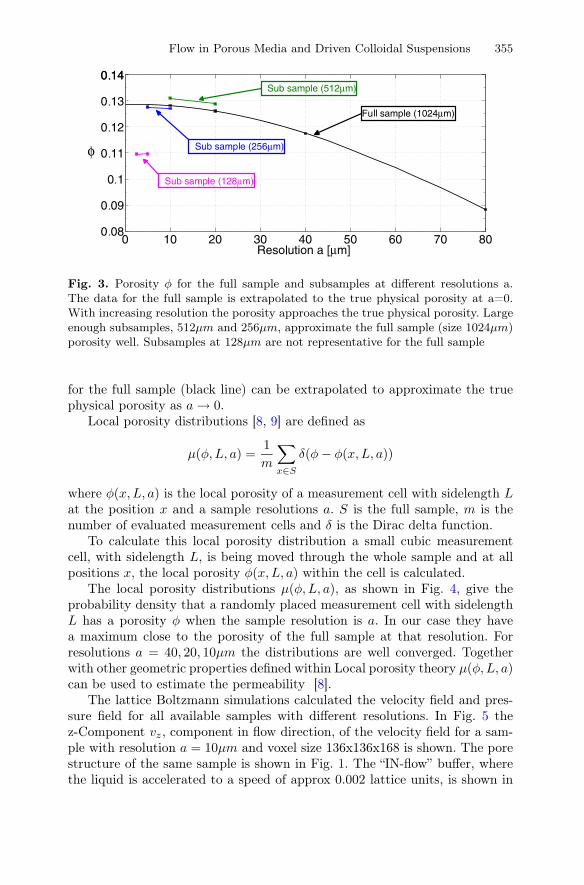
For each sample geometrical properties such as the porosity, specific surfaceand mean/total curvature have been calculated to investigate their behaviorwith changing resolution and subsampling. From the resolution dependentporosity φ(a) (Fig. 3) conclusions can be drawn which resolution ranges ap-proximate the true physical porosity well enough and thus, are suitable forsimulations. Increasing the resolution (lower a) beyond a certain point (hereapprox. a = 5−10μm) will not justify the increase in data and CPU time buton the other hand low resolutions (a = 50 − 80μm) will most likely not yieldrelevant simulation data, because not even the sample porosity is close to thetrue porosity of the physical sandstone. As can be seen in (Fig. 3), subsamplesmuch smaller than 256μm will not represent the full sample well. The data


Fig. 3. Porosity φ for the full sample and subsamples at different resolutions a.The data for the full sample is extrapolated to the true physical porosity at a=0.With increasing resolution the porosity approaches the true physical porosity. Largeenough subsamples, 512μm and 256μm, approximate the full sample (size 1024μm)porosity well. Subsamples at 128μm are not representative for the full sample

for the full sample (black line) can be extrapolated to approximate the truephysical porosity as a → 0.

Local porosity distributions [8, 9] are defined as

μ(φ, L, a) =1m

∑x∈S

δ(φ − φ(x, L, a))

where φ(x, L, a) is the local porosity of a measurement cell with sidelength Lat the position x and a sample resolutions a. S is the full sample, m is thenumber of evaluated measurement cells and δ is the Dirac delta function.

To calculate this local porosity distribution a small cubic measurementcell, with sidelength L, is being moved through the whole sample and at allpositions x, the local porosity φ(x, L, a) within the cell is calculated.

The local porosity distributions μ(φ, L, a), as shown in Fig. 4, give theprobability density that a randomly placed measurement cell with sidelengthL has a porosity φ when the sample resolution is a. In our case they havea maximum close to the porosity of the full sample at that resolution. Forresolutions a = 40, 20, 10μm the distributions are well converged. Togetherwith other geometric properties defined within Local porosity theory μ(φ, L, a)can be used to estimate the permeability [8].

The lattice Boltzmann simulations calculated the velocity field and pres-sure field for all available samples with different resolutions. In Fig. 5 thez-Component vz, component in flow direction, of the velocity field for a sam-ple with resolution a = 10μm and voxel size 136x136x168 is shown. The porestructure of the same sample is shown in Fig. 1. The “IN-flow” buffer, wherethe liquid is accelerated to a speed of approx 0.002 lattice units, is shown in


Fig. 4. Local porosity distributions for a measurement cell size L = 320μm atdifferent resolutions a. Very high resolutions (a = 5μm) yield bad statistics, atthe size of the measurement cell used here. The distributions for resolutions a =40, 20, 10μm are very similar in shape, the mean porosity changes according to Fig. 3

green at the top. All voxel with vz > 0 are shown in translucent blue. Thebrown isosurfaces depict areas where vz > 0.001 in lattice units, being half ofthe maximum speed in the “IN-flow” buffer. They represent channels where theliquid flows fast. The flow through the porous medium is not homogeneous,even if the porous medium is quite homogeneous at this resolution.

In addition to the geometric characterizations and the velocity fields highprecision permeability calculations (Tbl. 2) for all 83 samples have beenperformed and are now been critically analyzed for accuracy, to gain furtherinsight into their resolution dependence and thereby into the nature of fluidtransport within highly complex geometries.

Table 2. Selected permeability results of the full sample (1024μm) for different res-olutions. An relative error of 0.05 has been estimated, resulting from the inaccuracyof the velocity field, calculated by the LB-simulation

Resolution [μm] Permeability [μm2]40 1.7±0.04320 2.2±0.05510 1.9±0.047


Fig. 5. Z-Component of the velocity field. Fluid is accelerated in the IN-flowbuffer on top(green). Shown in translucent blue is the complete volume fraction withvz > 0. Darker regions correspond to smaller velocities. All areas with a velocitywith vz > 0.001 are shown as isosurfaces. Channels with large connected isosurfacesthus carry the main flow through the porous medium

2 Simulation of Optical Tweezer Experiments

A colloidal suspension is a mixture of a fluid and particles or droplets with alength scale of some nanometers to micrometers suspended in it. Colloids area common part of everyday life. Substances like paint, glue, milk, blood andfog are just some examples. Due to their technical applications, colloids arestudied in several disciplines, among them physics, chemistry, and engineer-ing.

Colloidal particles are too large to be affected directly by quantum me-chanical effects. On the other hand, they are still small enough to be affectedby thermal fluctuations. Therefore, colloidal suspensions are an interestingsystem to study thermodynamic phenomena like diffusion, phase transitionsand more rare phenomena like stochastic resonance and critical Casimir forces.In solid state physics, colloidal crystals are used as model systems to studydefect formation, crystal structures and melting. In contrast to many systemsin these fields, which are on the nanometer scale, colloidal suspensions canbe observed and manipulated directly using techniques like video microscopy,confocal microscopy, total internal reflection microscopy (TIRM) and opticaltweezers. This offers numerous possibilities to control these systems on a perparticle basis.


We study dynamical properties of colloidal suspensions using computersimulations. The advantage of simulations is that parameters can be con-trolled in ways that are not accessible in experiments. Also, in many cases,information is available that cannot be measured directly in a real system.Over the past decades, several simulation techniques have become available,which model different aspects of suspensions.

Methods like molecular dynamics and Brownian dynamics only model thedynamics of the suspended colloidal particles and handle the solvent implicitlyby adding simplified forces to mimic the solvents behavior. Other approacheslike lattice-Boltzmann models, dissipative particle dynamics and stochasticrotation dynamics simulate the complete fluid and couple it to suspendedparticles. While the first set of methods are computationally very efficient,more complicated hydrodynamic effects are usually not taken into account(polarization of the solvent). The methods that do simulate the full fluid fieldcan reproduce hydrodynamic effects, but achieving quantitative accuracy farfrom equilibrium is still a challenge. Here, we focus on the Brownian dynamicstechnique in order to be able to simulate very large systems with an affordableamount of CPU time.

The dynamics of driven suspensions can be examined by dragging a col-loidal particle through it. In this article we present our simulations of a particledragged through a colloidal crystal and a suspension of coiled polymers us-ing an optical tweezer. The focus of the optical tweezer is moved with time,thereby pulling the impurity along.

Optical tweezers trap a colloid (or even an atom) in the focus of a laserbeam: this is because a dielectric is always driven along the field gradient.They are a very important tool in soft condensed matter physics: colloids cannot only be trapped, they can also be moved around individually by movingthe focus of the laser beam. Thereby the colloidal system can be controlledwith an accuracy that would be impossible for an atomic system. The opticaltweezer is modeled with a harmonic potential, i.e. as if the impurity wereconnected with the trap center by an ideal spring.

The simulations are motivated by experiments performed by R. Dullensin the group of C. Bechinger in Stuttgart and C. Gutsche in the group ofF. Kremer in Leipzig, respectively. In both cases, the simulation parametersare chosen to reproduce the experimental conditions as closely as possible.

2.1 Simulation Setup

The experiments are simulated using a modified Brownian dynamics (BD)method which includes some of the hydrodynamics caused by the draggedcolloid, as explained in Ref. [11]. The colloids/polymers and the probe particleare modeled as hard spheres with their respective radii.

We use a rectangular simulation volume with periodic boundary conditionsin all three directions. Due to long range hydrodynamic interactions, large


systems are required in order to reduce finite size effects. Thus, we typicallyhandle several hundred thousand particles in a single simulation.

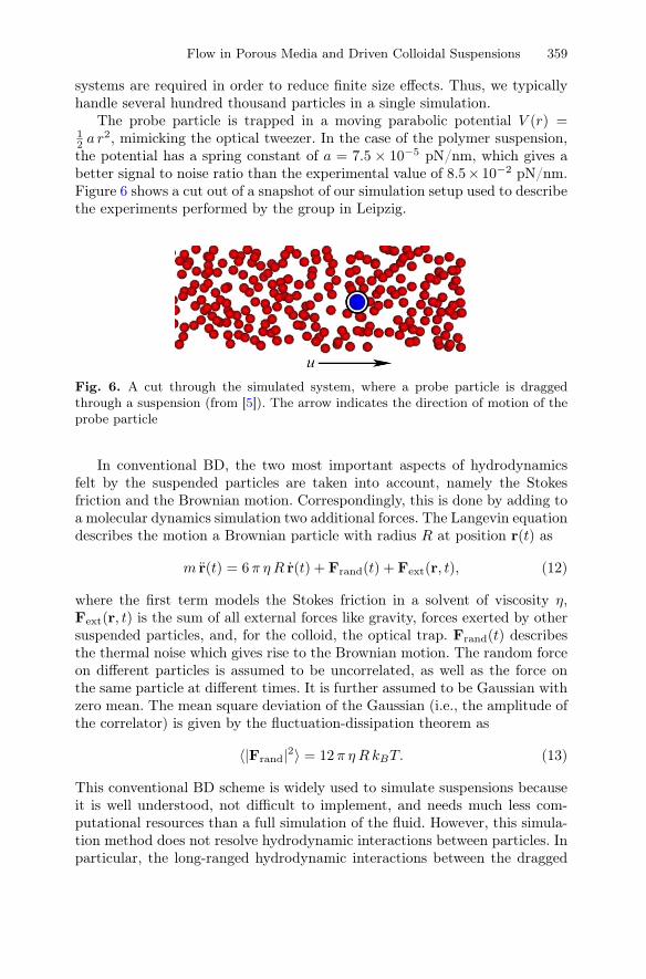
The probe particle is trapped in a moving parabolic potential V (r) =12 a r2, mimicking the optical tweezer. In the case of the polymer suspension,the potential has a spring constant of a = 7.5 × 10−5 pN/nm, which gives abetter signal to noise ratio than the experimental value of 8.5× 10−2 pN/nm.Figure 6 shows a cut out of a snapshot of our simulation setup used to describethe experiments performed by the group in Leipzig.

Fig. 6. A cut through the simulated system, where a probe particle is draggedthrough a suspension (from [5]). The arrow indicates the direction of motion of theprobe particle

In conventional BD, the two most important aspects of hydrodynamicsfelt by the suspended particles are taken into account, namely the Stokesfriction and the Brownian motion. Correspondingly, this is done by adding toa molecular dynamics simulation two additional forces. The Langevin equationdescribes the motion a Brownian particle with radius R at position r(t) as

m r(t) = 6 π η R r(t) + Frand(t) + Fext(r, t), (12)

where the first term models the Stokes friction in a solvent of viscosity η,Fext(r, t) is the sum of all external forces like gravity, forces exerted by othersuspended particles, and, for the colloid, the optical trap. Frand(t) describesthe thermal noise which gives rise to the Brownian motion. The random forceon different particles is assumed to be uncorrelated, as well as the force onthe same particle at different times. It is further assumed to be Gaussian withzero mean. The mean square deviation of the Gaussian (i.e., the amplitude ofthe correlator) is given by the fluctuation-dissipation theorem as

〈|Frand|2〉 = 12 π η R kBT. (13)

This conventional BD scheme is widely used to simulate suspensions becauseit is well understood, not difficult to implement, and needs much less com-putational resources than a full simulation of the fluid. However, this simula-tion method does not resolve hydrodynamic interactions between particles. Inparticular, the long-ranged hydrodynamic interactions between the dragged


colloid and the surrounding particles are not modeled. However, in the systemwe consider, these interactions are important, as the dragged colloid movesquickly and has a strong influence on the flow field around it. Therefore, theBD scheme is modified such that the effect caused by the flow field aroundthe dragged colloid is included. This is achieved by calculating the frictionforce on the small particles with radius Rc not with respect to a resting fluid(F = 6πηRcu), but with respect to the flow field caused by the moving colloid.The friction force then is

F = 6πηRc(u − v(r)), (14)

where v(r) is the flow field around the moving colloid at a position r withrespect to the colloid’s center. This correction leads to the inclusion of twohydrodynamics-mediated effects. Due to the large component of the flow fieldalong the direction of motion, both, in front and behind the probe, smallcolloids are dragged along. Also the flow of particles is advected around themoving probe particle, i.e., obstacles are moved out of the way to its sides.Both these effects lead to a reduction of drag force on the driven colloid.

2.2 Investigating the Stiffness and Occurrence of Defects inColloidal Crystals

To analyze the effects of the disturbance due to the dragged probe particle, wecan either measure the distance that the probe stays behind the focus of theoptical tweezer - and thereby the force required to drag the impurity throughthe crystal - or examine the reaction of the crystal itself. With our simulationswe show that in a colloidal crystal, the velocity-force relation for the draggedcolloidal particle is close to linear despite the complicated surrounding. It isalso shown that the inter-colloid potential does have an influence on the dragforce, though not as strong as velocity. This is one example of a result thatcould not be obtained easily in experiments. Using maps of average particledensity and defect distributions, we illustrate the effect of the dragged colloidalparticle on the crystal structure.

An example of a rather small system is given in Fig. 7. For large tweezervelocities, much larger crystals are needed and for studying the relaxation ofthe crystal, we also have to simulate for at least a 100 to 300 seconds of realtime causing these simulations to cost up to a few thousand CPU hours each.

2.3 Dragging a Colloidal Probe Through a Polymer Suspension

The second system we consider is a suspension of coiled polymers which aremodeled as hard spheres. A colloidal particle is dragged through the suspen-sion at high velocities. In the experiment and in the simulation, a drag force ismeasured that is higher than that calculated from the suspension’s viscosity asobtained from a shear rheometer. This increase in drag force can be explained


Fig. 7. Simulation of a large colloidal particle dragged through a crystal consistingof smaller colloids by means of an optical tweezer. The coloring denotes defectsoccurring due to the distortion of the crystal

by a jamming of polymers in front of the moving colloidal particle. In contrastto experiments, this jamming can be observed directly in computer simula-tions as the positions of the polymers are available. The simulation resultsare compared to dynamic density functional theory calculations by Rauscheret. al and experimental results by Gutsche et al.. A very good quantitativeagreement between experiment, theory and simulation is observed [5].

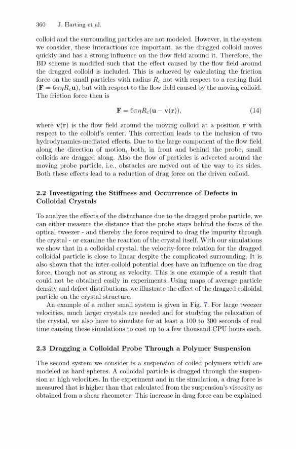
From the simulation data, it is possible to measure the effective polymerconcentration around the dragged colloid. To accomplish this, we take about2000 two dimensional slices of the simulation and move each snapshot suchthat the position of the colloid coincides in each snapshot. We calculate theprobability for each of the 200 × 200 bins to be occupied by a polymer byaveraging over all snapshots. Polymers accumulate in front of the colloidalparticle and the concentration in the back is reduced due to the finite Pecletnumber of the polymers. For high polymer concentrations, the probability tofind a polymer in front of the colloid is close to one. The region right behindthe colloid is almost clear of polymers, because the polymers get advectedaway from the colloid before they can diffuse into this region.

Our model reproduces very well the experimentally found linear relationbetween drag force and the drag velocity for different polymer concentrations.As higher drag velocities require a larger system (even with periodic boundaryconditions) and short numerical time steps, we are limited to about 80 μm/sby the available computational resources and time. However, the linearity ofthe drag force with respect to the velocity at high enough velocities allows toextrapolate to the higher velocities used in the experiments.


Fig. 8. Polymer density around the colloidal particle averaged over 2000 snapshotsof the system. Lighter colors correspond to higher polymer densities. Also visible aredensity oscillations in front of the colloid, which are characteristic for hard spheresystems

3 Conclusion

In this report we have presented results from lattice Boltzmann simulationsof fluid flow in porous media and the simulation of optical tweezer experi-ments. In particular the AMD Opteron cluster in Karlsruhe has been foundto perform particularly well with our simulation codes. In the case of porousmedia simulations we have demonstrated that we are able to systematicallydetermine the permeability of digitized quartzitic sandstone samples – even ifthe resolution of the samples is very high resulting in the need of substantialcomputational resources.

In the second part of this article we reported on our Brownian dynamicssimulations of optical tweezer experiments, where a large probe particle istrapped by a laser beam and dragged either through a colloidal crystal orthrough a polymer suspension. In both cases, quantitative agreement withexperimental data was observed.

Acknowledgments

We are grateful to the High Performance Computing Center in Stuttgartand the Scientific Supercomputing Center in Karlsruhe for providing accessto their NEC SX-8 and HP 4000 machines. We would like to thank BibhuBiswal, Peter Diez, and Frank Raischel for fruitful discussions. This work wassupported by the collaborative research center 716 and the DFG program“nano- and microfluidics”.

References

1. P.L. Bhatnagar, E.P. Gross, and M. Krook. Model for collision processes in gases.I. small amplitude processes in charged and neutral one-component systems.Phys. Rev., 94(3):511, 1954.


2. B. Biswal, P.E. Oren, R. Held, S. Bakke, and R. Hilfer. Stochastic multiscalemodel for carbonate rocks. Phys.Rev. E, 75:061303, 2007.

3. S. Chapman and T.G. Cowling. The mathematical theory of non-uniform gases.Cambridge University Press, second edition, 1952.

4. U. Frisch, D. d’Humiéres, B. Hasslacher, P. Lallemand, Y. Pomeau, and J.P.Rivet. Lattice gas hydrodynamics in two and three dimensions. Complex Sys-tems, 1(4):649, 1987.

5. C. Gutsche, F. Kremer, M. Krüger, M. Rauscher, J. Harting, and R. Weeber.Colloids dragged through a polymer solution: experiment, theory and simula-tion. Submitted for publication, arXiv:0709.4142, 2007.

6. J. Harting, M. Harvey, J. Chin, M. Venturoli, and P.V. Coveney. Large-scalelattice Boltzmann simulations of complex fluids: advances through the adventof computational grids. Phil. Trans. R. Soc. Lond. A, 363:1895–1915, 2005.

7. 2003. HDF5 – a general purpose library and file format for storing scientificdata, http://hdf.ncsa.uiuc.edu/HDF5.

8. R. Hilfer. Transport and relaxation phenomena in porous media. Adv. Chem.Phys., XCII:299, 1996.

9. R. Hilfer. Local porosity theory and stochastic reconstruction for porous media.In K. Mecke and D. Stoyan, editors, Statistical Physics and Spatial Statistics,volume 554 of Lecture Notes in Physics, page 203, Berlin, 2000. Springer.

10. A.J.C. Ladd and R. Verberg. Lattice-boltzmann simulations of particle-fluidsuspensions. J. Stat. Phys., 104(5):1191, 2001.

11. M. Rauscher, M. Krüger, A. Dominguez, and F. Penna. A dynamic densityfunctional theory for particles in a flowing solvent. J. Chem. Phys., 127:244906,2007.

http://arxiv.org/abs/arXiv:0709.4142

http://hdf.ncsa.uiuc.edu/HDF5

numerical modeling of fluid flow in porous media and in driven colloidal...

Documents