TRC Report # 11-008 | Syrrakou and Pinder | October 2011

A Report from the University of Vermont Transportation Research Center

Numerical Modeling and Experimental Investigation of the Local Hydrology of a

Porous Concrete Site

Numerical Modeling and Experimental Investigation of the Local Hydrology of a Porous

Concrete Site

By Christina Syrrakou and George Pinder

Project Collaborators: Jennifer Fitch, Thomas Eliassen, William Ahearn

Project funded by the Vermont Agency of Transportation and UVM Transportation Research Center

October, 2011

University of Vermont College of Engineering and Mathematical Sciences

Department of Civil and Environmental and Engineering

UVM TRC #11-008

This project was funded by the Vermont Agency of Transportation (Vtrans) and the UVMTransportation Research Center (UVM TRC). The authors would like to acknowledge Dr.Dewoolkar and his students: Mark Suozzo, Ian Anderson, Lalita Oka and Jaron Borg fortheir help during the field visits and in the lab. In addition, we acknowledge Dylan Burnsfor providing the equipment for the evaporation experiments and Floyd Vilmont for his helpin manufacturing the water-retention cells and overall input in the mechanical issues of thisproject. Finally, the authors wish to thank Vtrans and especially Jeniffer Fitch, JasonTrembley, Philip Dessureau, Thomas Eliassen and William Ahearn for providing data andtheir valuable cooperation through the course of this project.

i

UVM TRC #11-008

Contents

1 Introduction 1

2 State of Knowledge 2

2.1 Interaction of porous concrete utilization and hydrology . . . . . . . . . . . 2

2.1.1 Review of studies focusing on site monitoring with respect to runoffand infiltration . . . . . . . . . . . . . . . . . . . . . . . . . . . . . . 2

2.1.2 Review of studies focusing on retention and evaporation . . . . . . . 3

2.2 Porous pavement models . . . . . . . . . . . . . . . . . . . . . . . . . . . . . 4

2.2.1 Review of commercial porous pavement models to date . . . . . . . 4

2.3 Open Questions . . . . . . . . . . . . . . . . . . . . . . . . . . . . . . . . . . 5

3 Research Approach and Methods 6

3.1 Field Investigation . . . . . . . . . . . . . . . . . . . . . . . . . . . . . . . . 6

3.1.1 Site Description . . . . . . . . . . . . . . . . . . . . . . . . . . . . . . 6

3.1.2 Site Instrumentation . . . . . . . . . . . . . . . . . . . . . . . . . . . 8

3.1.3 Site Geology . . . . . . . . . . . . . . . . . . . . . . . . . . . . . . . 9

3.2 Laboratory procedures . . . . . . . . . . . . . . . . . . . . . . . . . . . . . . 13

3.2.1 Grain size distribution analysis . . . . . . . . . . . . . . . . . . . . . 13

3.2.2 Water retention curve for glacial till . . . . . . . . . . . . . . . . . . 14

3.3 Retention and subsequent evaporation of stormwater . . . . . . . . . . . . . 17

4 Mathematical Model 21

4.1 Runoff on pavement module . . . . . . . . . . . . . . . . . . . . . . . . . . . 22

4.1.1 Example . . . . . . . . . . . . . . . . . . . . . . . . . . . . . . . . . . 24

4.2 VTC Module . . . . . . . . . . . . . . . . . . . . . . . . . . . . . . . . . . . 25

4.2.1 Example . . . . . . . . . . . . . . . . . . . . . . . . . . . . . . . . . . 26

4.3 Retention and evaporation of water in the gravel . . . . . . . . . . . . . . . 29

4.3.1 Example . . . . . . . . . . . . . . . . . . . . . . . . . . . . . . . . . . 29

4.4 Discussion . . . . . . . . . . . . . . . . . . . . . . . . . . . . . . . . . . . . . 30

ii

UVM TRC #11-008

5 The Field Experiment 32

5.1 Reason behind the experiment . . . . . . . . . . . . . . . . . . . . . . . . . 32

5.2 The day of the experiment . . . . . . . . . . . . . . . . . . . . . . . . . . . . 32

5.3 Results . . . . . . . . . . . . . . . . . . . . . . . . . . . . . . . . . . . . . . . 33

5.3.1 Water Levels . . . . . . . . . . . . . . . . . . . . . . . . . . . . . . . 33

5.3.2 Hurricane Irene . . . . . . . . . . . . . . . . . . . . . . . . . . . . . . 37

5.3.3 Conductivity Measurements . . . . . . . . . . . . . . . . . . . . . . . 40

5.3.4 Drain and flushing basin information . . . . . . . . . . . . . . . . . . 43

5.4 Discussion . . . . . . . . . . . . . . . . . . . . . . . . . . . . . . . . . . . . . 46

6 General Discussion 47

Appendices 51

A 100-series wells 51

B 200-series wells 58

C 300-series wells 67

D The Noordbergum effect 76

iii

UVM TRC #11-008

List of Figures

3.1 Site design . . . . . . . . . . . . . . . . . . . . . . . . . . . . . . . . . . . . . 7

3.2 The Randolph Park and Ride porous concrete parking lot . . . . . . . . . . 8

3.3 Monitoring Wells . . . . . . . . . . . . . . . . . . . . . . . . . . . . . . . . . 9

3.4 Groundwater response during rainfall events (11/19/10 to 12/8/10). . . . . 10

3.5 Winter 2011 groundwater level data . . . . . . . . . . . . . . . . . . . . . . 10

3.6 Artesian well setup . . . . . . . . . . . . . . . . . . . . . . . . . . . . . . . . 11

3.7 Location of tetrahedra on the site’s map . . . . . . . . . . . . . . . . . . . . 12

3.8 Grain Size Distribution curve for a soil core obtained in the field . . . . . . 13

3.9 Water Retention Curve Experimental Apparatus . . . . . . . . . . . . . . . 16

3.10 Water Retention Curve results . . . . . . . . . . . . . . . . . . . . . . . . . 16

3.11 Experimental setup for evaporation experiment . . . . . . . . . . . . . . . . 17

3.12 Detail of Experimental setup . . . . . . . . . . . . . . . . . . . . . . . . . . 18

3.13 Evaporation experiment results for Tests 1, 2 and 3. Test 2 and 3 showcombination of data obtained through the computer and on the load celldisplay. . . . . . . . . . . . . . . . . . . . . . . . . . . . . . . . . . . . . . . 19

3.14 Evaporation experiment results for Test 4. Temperature and relative humid-ity was also monitored during this Test. . . . . . . . . . . . . . . . . . . . . 19

4.1 Physical processes taking place in a porous concrete system . . . . . . . . . 22

4.2 Results - Part 1 . . . . . . . . . . . . . . . . . . . . . . . . . . . . . . . . . . 24

4.3 Results - Part 2 . . . . . . . . . . . . . . . . . . . . . . . . . . . . . . . . . . 25

4.4 Layer setup in VTC . . . . . . . . . . . . . . . . . . . . . . . . . . . . . . . 26

4.5 Simulation results in Layer 10 (top layer) . . . . . . . . . . . . . . . . . . . 27

4.6 Simulation results in Layer 7 . . . . . . . . . . . . . . . . . . . . . . . . . . 28

4.7 Simulation results in Layer 5 . . . . . . . . . . . . . . . . . . . . . . . . . . 28

4.8 Model results simulating flow through coarse stone and evaporation (a) . . 30

4.9 Model results simulating flow through coarse stone and evaporation (b) . . 30

5.1 Water Levels in SP1. . . . . . . . . . . . . . . . . . . . . . . . . . . . . . . . 34

5.2 Water Levels in SP2. . . . . . . . . . . . . . . . . . . . . . . . . . . . . . . . 34

iv

UVM TRC #11-008

5.3 Water Levels in SP3. . . . . . . . . . . . . . . . . . . . . . . . . . . . . . . . 35

5.4 Water Levels in 200-series wells (right site area). . . . . . . . . . . . . . . . 35

5.5 Water Levels in 200-series wells (left site area). . . . . . . . . . . . . . . . . 36

5.6 Water Levels in 300-series wells (part a). . . . . . . . . . . . . . . . . . . . . 36

5.7 Water Levels in 300-series wells (part b). . . . . . . . . . . . . . . . . . . . . 37

5.8 Water Levels in 300-series wells (part a) - Irene response. . . . . . . . . . . 38

5.9 Water Levels in 300-series wells (part b) - Irene response. . . . . . . . . . . 38

5.10 Water Levels in 200-series wells (part a) - Irene response. . . . . . . . . . . 39

5.11 Water Levels in 200-series wells (part b) - Irene response. . . . . . . . . . . 39

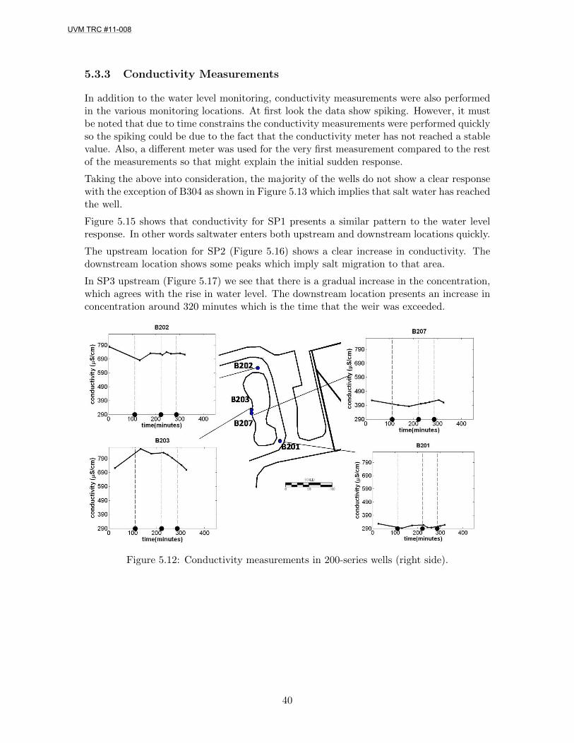
5.12 Conductivity measurements in 200-series wells (right side). . . . . . . . . . 40

5.13 Conductivity measurements in 300-series wells (part a). . . . . . . . . . . . 41

5.14 Conductivity measurements in 300-series wells (part b). . . . . . . . . . . . 41

5.15 Conductivity measurements in SP1. . . . . . . . . . . . . . . . . . . . . . . 42

5.16 Conductivity measurements in SP2. . . . . . . . . . . . . . . . . . . . . . . 42

5.17 Conductivity measurements in SP3. . . . . . . . . . . . . . . . . . . . . . . 43

5.18 Water level and conductivity measurements in flushing basin. . . . . . . . . 44

5.19 Superposition of water level measurements in flushing basin on SP3 data. . 44

5.20 Location of openings on perimeter drain . . . . . . . . . . . . . . . . . . . . 45

v

UVM TRC #11-008

List of Tables

3.1 Pressure in artesian wells (in inches oh H20) . . . . . . . . . . . . . . . . . . 11

3.2 Groundwater gradient : Coordinates and calculations . . . . . . . . . . . . . 12

3.3 Evaporation Test Results . . . . . . . . . . . . . . . . . . . . . . . . . . . . 19

5.1 Conductivity measurements in perimeter drain openings . . . . . . . . . . . 45

vi

UVM TRC #11-008

Chapter 1

Introduction

Although porous pavement use has been accepted as a successful stormwater managementpractice in warm climates, application in regions with colder climates, like New England, isstill under investigation. The Randolph Park and Ride Site, which is the area of interest ofthis specific study, is the first porous concrete site constructed in Vermont. The site, whichwas built in 2008 and is under use up to today, is quite unique in terms of the geology ofthe underlying materials and also the extensive instrumentation that has been applied inthe field. The purpose of building this site was in part “commercial”, to provide the townof Randolph with a public parking lot, and part “experimental”, aiming at giving insightto the optimal design of porous pavements in New England. This study focuses on theexperimental use of the site.

More specifically, this study initially aims at investigating the interaction between porousconcrete utilization and local hydrology at porous concrete sites in New England. With thispart achieved, a mathematical model can be developed and used prior to construction as adesign tool for other porous concrete sites. The final model will take into account a varietyof physical processes and treat the system as a whole, starting from rainfall falling on thetop of the porous concrete, to the point where water meets the groundwater system. It isalso a secondary goal of this study to combine the mathematical model created with anoptimization algorithm that will allow for optimal design of porous concrete sites in termsof minimal expense.Therefore the key goals of this study are the following.

• Investigate the local hydrology and understand the geologic characteristics of the soilin the Randolph Site.

• Enhance knowledge of field observations through laboratory experiments and deter-mine the parameters needed by the mathematical model.

• Create a mathematical model that incorporates all the different processes taking placein a porous concrete system.

• Use the constructed model to evaluate the site design.

• Use the model in combination with an optimization code to provide the optimal designin terms of least cost.

• Extend the use of the resulting model for other sites.

1

UVM TRC #11-008

Chapter 2

State of Knowledge

The use of porous concrete for its reduced environmental impact started in the 1970s inFlorida [8]. Besides porous concrete, which is the main focus here, other kinds of permeablepavement installations include porous asphalt and various kinds of pavers.

The following literature review aims at providing a general background on existing porouspavement studies with emphasis placed on the hydrologic impact of porous concrete.

2.1 Interaction of porous concrete utilization and hydrology

2.1.1 Review of studies focusing on site monitoring with respect to runoffand infiltration

In a study by Bean et al. [3], four permeable pavement applications (consisting of porousconcrete, concrete grid pavers and permeable interlocking concrete pavers) were monitoredin order to determine effectiveness in terms of reducing runoff quantity and improvingwater quality. Hardware instrumentation allowed detailed runoff and rainfall measurementsin time and the study results showed that runoff was not only reduced but for some eventseven eliminated.

Kwiatkowski [17], describes a hydrologic study on a porous concrete site on campus atVillanova University. There, porous concrete was overlaid on storage beds filled with coarseaggregate, on top of a sandy-silt well draining soil. The specific study although mostlyfocused on water quality data, describes the ability of the site to accept a significant amountof infiltration from surrounding areas and reduce runoff as well. In this study it is alsomentioned that the porous concrete area was later reduced by paving over part of it withconventional concrete, but the sites overall performance still remained satisfactory.

Another study on porous concrete sites, with more general focus, is from Henderson andTighe [11] who performed a research study on five porous concrete test areas in Canada inorder to test concrete strength characteristics during freeze-thaw cycles. Also, a universityresearch study in Auburn, Alabama, presents five porous concrete projects constructed anddesigned by students in collaboration with professors, inside the campus area to monitorsite performance regarding concrete failure and infiltration of rainfall [10].

For an additional review on porous concrete installations the reader can also refer to Fer-guson [8]. His review contains a comparison of successful and unsuccessful installations in

2

UVM TRC #11-008

close proximity locations, installations on sandy or fine-grained soils and finally installationson the west coast or towards colder climates.

Studies on other types of porous pavement with emphasis on the sites hydrologic charac-teristics are from Brattebo and Booth [4], who studied the long-term effectiveness of fourpermeable pavement parking lots consisting of block pavers, in terms of stormwater quan-tity and quality and Fassman and Blackbourne [7] who monitored runoff from a permeablepavement roadway site on a relatively impermeable subgrade soil in New Zealand for aperiod of two years. In the latter study, the sites design incorporated an underdrain systemto collect water stored in the crushed stone layer and also took into account retention ofwater and subsequent evaporation into the atmosphere.

On a slightly different note, installation of porous pavement on clayey soils has been studiedby Dreelin et al. [6], who tested the effectiveness of a porous pavement consisting of grasspavers during natural storm events and found that stormwater was actually being infiltratedinto the clayey subgrade material. Also, the behaviour of porous pavement in cold climateswas the research focus of a study by Backstrom [2]. Temperature of porous pavementduring freezing and thawing was monitored on a porous asphalt site in northern Sweden.This study is actually one of the few found in the literature where the groundwater table ismonitored carefully through the period of analysis and shows how the groundwater changescompared to the rest of the monitoring area.

2.1.2 Review of studies focusing on retention and evaporation

The idea of evaporation of water inside the porous pavement’s coarse stone storage areahas been addressed by Andersen et al. [1]. Results of their study showed that an averageof 55 percent of a one hour duration 15 mm rainfall could be retained by an initially drystructure and 30 percent of a similar rainfall by an initially wet structure. Also, evaporationlosses proved to be dependent on the environmental conditions and the grain size of thesubstrate. Small grain sizes showed lower drainage from the bottom of the structure andhigher evaporation rates.

Also, Kunzen [16] measured evaporation processes inside a column filled with porous con-crete and sand using pressure probes and used a mass balance approach to calculate evapo-ration. In another study by Fassman and Blackbourne [7], losses of water inside the subbaseof a block-pavers porous pavement were also attributed to evaporation losses. Finally, long-term evaporation of water inside a porous pavement parking lot in Spain was mentioned ina study by Gomez-Ullate et al. [9], although their study mostly focused on the influence ofthe geotextile on water retention in pervious pavements.

3

UVM TRC #11-008

2.2 Porous pavement models

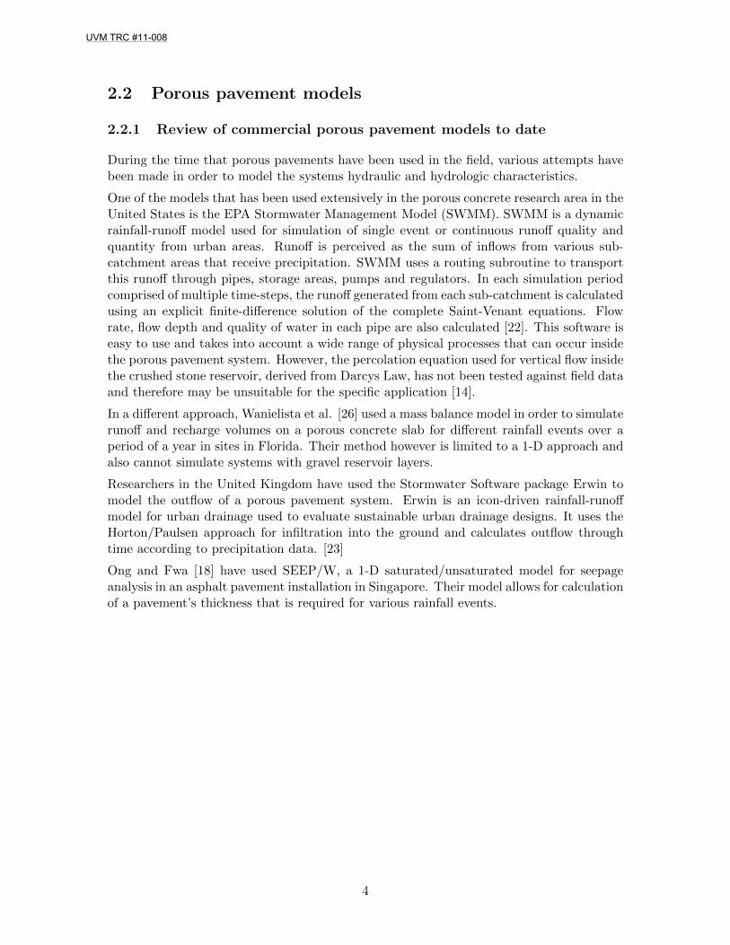
2.2.1 Review of commercial porous pavement models to date

During the time that porous pavements have been used in the field, various attempts havebeen made in order to model the systems hydraulic and hydrologic characteristics.

One of the models that has been used extensively in the porous concrete research area in theUnited States is the EPA Stormwater Management Model (SWMM). SWMM is a dynamicrainfall-runoff model used for simulation of single event or continuous runoff quality andquantity from urban areas. Runoff is perceived as the sum of inflows from various sub-catchment areas that receive precipitation. SWMM uses a routing subroutine to transportthis runoff through pipes, storage areas, pumps and regulators. In each simulation periodcomprised of multiple time-steps, the runoff generated from each sub-catchment is calculatedusing an explicit finite-difference solution of the complete Saint-Venant equations. Flowrate, flow depth and quality of water in each pipe are also calculated [22]. This software iseasy to use and takes into account a wide range of physical processes that can occur insidethe porous pavement system. However, the percolation equation used for vertical flow insidethe crushed stone reservoir, derived from Darcys Law, has not been tested against field dataand therefore may be unsuitable for the specific application [14].

In a different approach, Wanielista et al. [26] used a mass balance model in order to simulaterunoff and recharge volumes on a porous concrete slab for different rainfall events over aperiod of a year in sites in Florida. Their method however is limited to a 1-D approach andalso cannot simulate systems with gravel reservoir layers.

Researchers in the United Kingdom have used the Stormwater Software package Erwin tomodel the outflow of a porous pavement system. Erwin is an icon-driven rainfall-runoffmodel for urban drainage used to evaluate sustainable urban drainage designs. It uses theHorton/Paulsen approach for infiltration into the ground and calculates outflow throughtime according to precipitation data. [23]

Ong and Fwa [18] have used SEEP/W, a 1-D saturated/unsaturated model for seepageanalysis in an asphalt pavement installation in Singapore. Their model allows for calculationof a pavement’s thickness that is required for various rainfall events.

4

UVM TRC #11-008

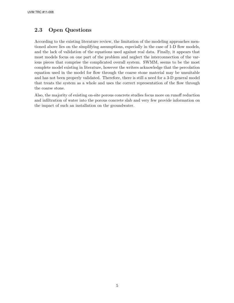
2.3 Open Questions

According to the existing literature review, the limitation of the modeling approaches men-tioned above lies on the simplifying assumptions, especially in the case of 1-D flow models,and the lack of validation of the equations used against real data. Finally, it appears thatmost models focus on one part of the problem and neglect the interconnection of the var-ious pieces that comprise the complicated overall system. SWMM, seems to be the mostcomplete model existing in literature, however the writers acknowledge that the percolationequation used in the model for flow through the coarse stone material may be unsuitableand has not been properly validated. Therefore, there is still a need for a 3-D general modelthat treats the system as a whole and uses the correct representation of the flow throughthe coarse stone.

Also, the majority of existing on-site porous concrete studies focus more on runoff reductionand infiltration of water into the porous concrete slab and very few provide information onthe impact of such an installation on the groundwater.

5

UVM TRC #11-008

Chapter 3

Research Approach and Methods

As mentioned previously, this research is focused on a specific porous concrete site calledRandolph Park and Ride located in the town of Randolph, Vermont. The site has operatedas a public parking lot facility since 2008 and is the first porous concrete site built inVermont. At the onset of this research, in the beginning of Fall 2008, the site was alreadydesigned and under construction. At that point, the authors, in collaboration with Vtrans(the agency responsible for building the site), decided the location of a set of monitoringwells.

The specific project reported upon herein is the combination of three interconnected pieces.

• The field investigation

• the laboratory procedures

• and finally the mathematical model.

The field investigation part is a key part of this study. The main problem of porouspavement studies is the lack of the model’s calibration according to field data. The factthat the Randolph site is equipped with a number of monitoring wells and scientific equip-ment is a significant advantage of this study. The laboratory procedures part helps tostrengthen knowledge of the field conditions. Finally, all data that derive from both thefield investigation and the laboratory experiments serve as an input to the mathematicalmodel, which is the final and most important piece of this research.

3.1 Field Investigation

3.1.1 Site Description

The field-test site is located at the intersection of VT Route 66 and T.H. 46 in the town ofRandolph, Vermont. The area of interest is the porous concrete parking lot. The broaderarea also includes a conventional asphalt road section. As mentioned previously, the facilityhas been in use since the fall of 2008. During the second year of operation the first signsof deterioration of the porous concrete area became evident. The deterioration continuedand became worse during the 3rd year of operation. A solution for this issue is yet to

6

UVM TRC #11-008

be determined. However, Vtrans early on suggested that there is a possibility of pavingover the failing areas with conventional concrete. If this were the case, runoff from theconventionally paved areas would result in a recharge term on the porous concrete surface.

The porous concrete slab parking area is 36,000 ft2 and consists of 6 inches of perviousconcrete, underlain by 2 inches of AASHTO No. 57 crushed stone and 34 inches minimumof AASHTO No. 2 crushed stone which, in combination, forms the reservoir where watercan be stored before infiltration into the subsurface. A woven geotextile fabric is located atthe bottom of the No.2 stone to prevent migration of the subgrade soil inside the stone. Inaddition to that, an underdrain system is installed inside the reservoir. This system is ableto collect the water that infiltrates through the porous concrete into special ’boxes’ calleddrop inlets and from there direct it to a retention pond away from the porous concrete slab.Water can be measured inside the inlets and provide insight on the amount infiltrated intothe system. One of the reasons that the underdrain system was incorporated in the designis the extremely low permeability of the underlying soil. Underdrains in this case makesure that the porous concrete does not overflood after an intense rainfall. In addition, theunderdrain system was incorporated in case the porous concrete concept failed. In thatcase, the area could be paved over with conventional concrete but still meet the stormwaterregulations for the town of Randolph. Figure 3.1 shows the site design. In addition to theunderdrains, the site is also equipped with a perforated pipe located along the perimeter ofthe porous concrete area. The usage of this ”perimeter drain” is to collect any amount ofrunoff from the surrounding site area.

(a) Cross sectional sequence of materials (b) Underdrain design

Figure 3.1: Site design

Vtrans has been monitoring water level data inside the drop inlets over time. However,the initially collected data showed that, strangely enough, water levels in the drop inletsremained stable and relatively unaffected by the rainfall events. Since the drop inlets aresupposed to collect any amount of water infiltrated into the porous pavement that does

7

UVM TRC #11-008

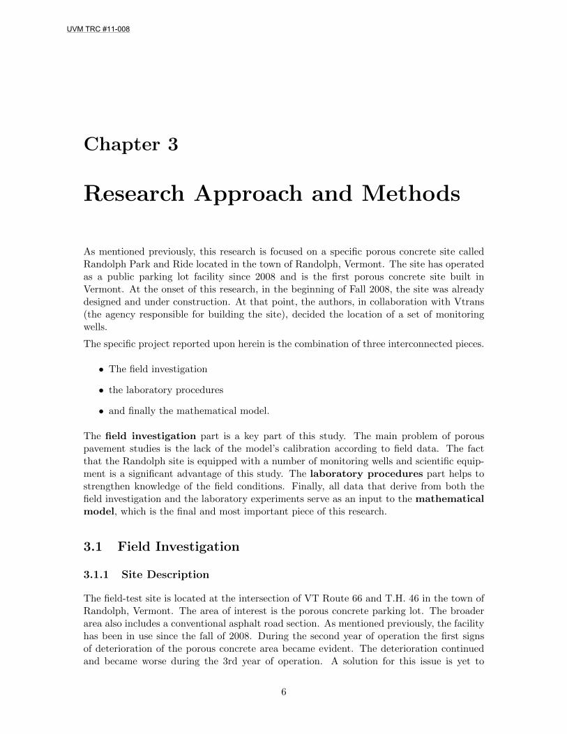
not infiltrate the soil, and the subgrade soil is quite impermeable prohibiting infiltrationof water, questions arose as to where the water is actually going. This was a mysteriousphenomenon in the field and up to this day a solid answer has not been provided. Varioushypotheses have been made, the most dominant being water could be retained by thecrushed stone surface and then evaporate into the atmosphere. Another hypothesis is thatwater that inflitrates the porous concrete slab could somehow leak towards the ”perimeterdrain” and therefore fail to flow towards the underdrains in the subbase.

Figure 3.2: The Randolph Park and Ride porous concrete parking lot

3.1.2 Site Instrumentation

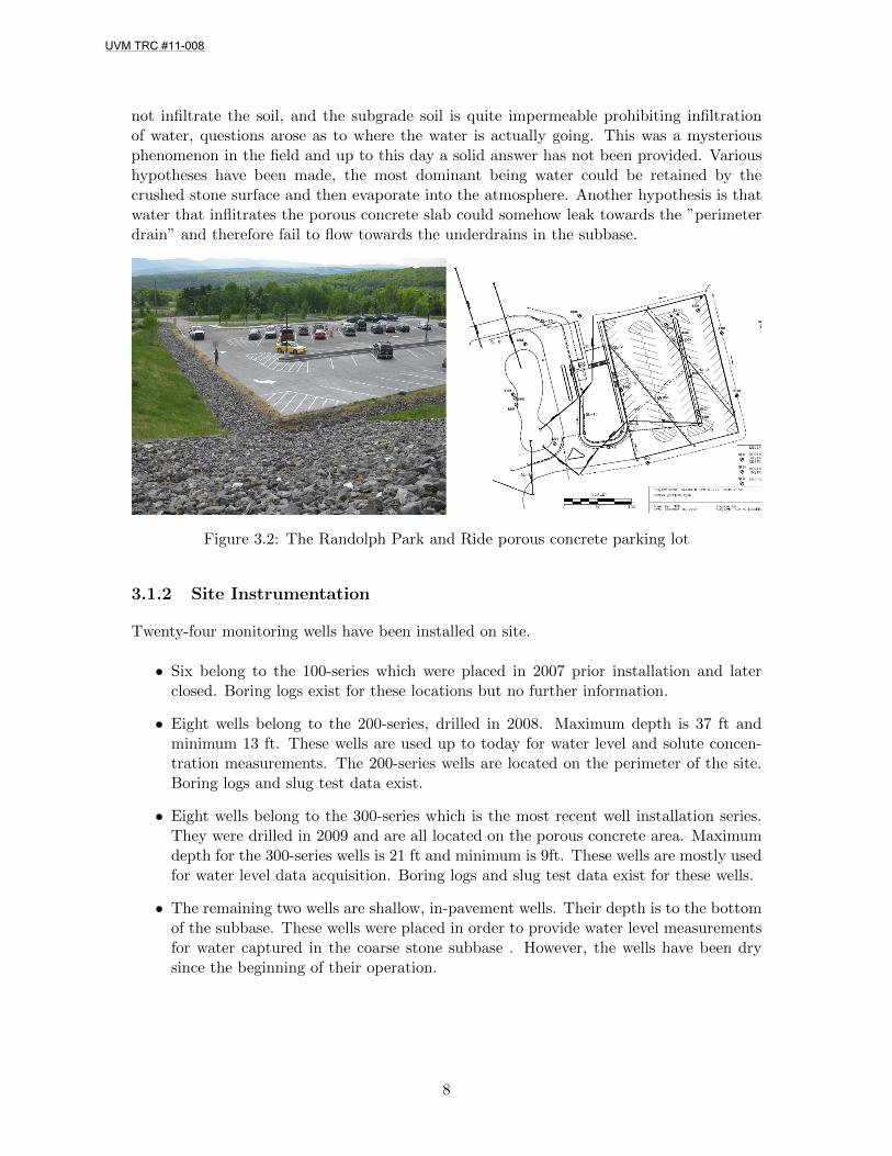
Twenty-four monitoring wells have been installed on site.

• Six belong to the 100-series which were placed in 2007 prior installation and laterclosed. Boring logs exist for these locations but no further information.

• Eight wells belong to the 200-series, drilled in 2008. Maximum depth is 37 ft andminimum 13 ft. These wells are used up to today for water level and solute concen-tration measurements. The 200-series wells are located on the perimeter of the site.Boring logs and slug test data exist.

• Eight wells belong to the 300-series which is the most recent well installation series.They were drilled in 2009 and are all located on the porous concrete area. Maximumdepth for the 300-series wells is 21 ft and minimum is 9ft. These wells are mostly usedfor water level data acquisition. Boring logs and slug test data exist for these wells.

• The remaining two wells are shallow, in-pavement wells. Their depth is to the bottomof the subbase. These wells were placed in order to provide water level measurementsfor water captured in the coarse stone subbase . However, the wells have been drysince the beginning of their operation.

8

UVM TRC #11-008

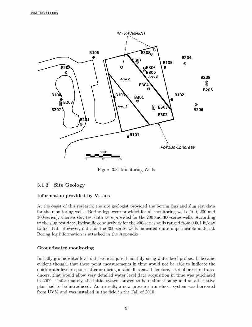
Figure 3.3: Monitoring Wells

3.1.3 Site Geology

Information provided by Vtrans

At the onset of this research, the site geologist provided the boring logs and slug test datafor the monitoring wells. Boring logs were provided for all monitoring wells (100, 200 and300-series), whereas slug test data were provided for the 200 and 300-series wells. Accordingto the slug test data, hydraulic conductivity for the 200-series wells ranged from 0.001 ft/dayto 5.6 ft/d. However, data for the 300-series wells indicated quite impermeable material.Boring log information is attached in the Appendix.

Groundwater monitoring

Initially groundwater level data were acquired monthly using water level probes. It becameevident though, that these point measurements in time would not be able to indicate thequick water level response after or during a rainfall event. Therefore, a set of pressure trans-ducers, that would allow very detailed water level data acquisition in time was purchasedin 2009. Unfortunately, the initial system proved to be malfunctioning and an alternativeplan had to be introduced. As a result, a new pressure transducer system was borrowedfrom UVM and was installed in the field in the Fall of 2010.

9

UVM TRC #11-008

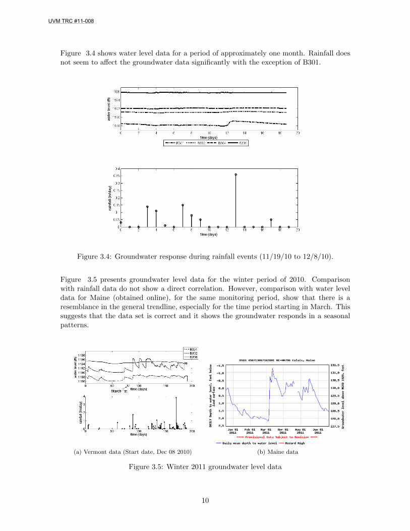
Figure 3.4 shows water level data for a period of approximately one month. Rainfall doesnot seem to affect the groundwater data significantly with the exception of B301.

Figure 3.4: Groundwater response during rainfall events (11/19/10 to 12/8/10).

Figure 3.5 presents groundwater level data for the winter period of 2010. Comparisonwith rainfall data do not show a direct correlation. However, comparison with water leveldata for Maine (obtained online), for the same monitoring period, show that there is aresemblance in the general trendline, especially for the time period starting in March. Thissuggests that the data set is correct and it shows the groundwater responds in a seasonalpatterns.

(a) Vermont data (Start date, Dec 08 2010) (b) Maine data

Figure 3.5: Winter 2011 groundwater level data

10

UVM TRC #11-008

Direction of groundwater flow

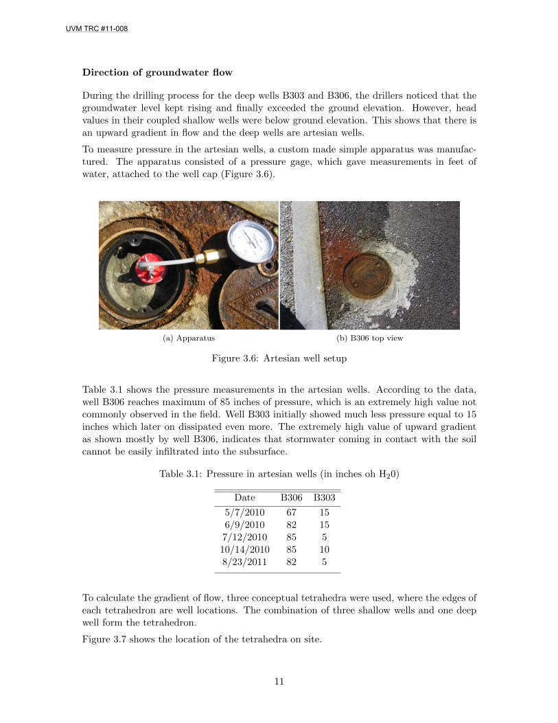
During the drilling process for the deep wells B303 and B306, the drillers noticed that thegroundwater level kept rising and finally exceeded the ground elevation. However, headvalues in their coupled shallow wells were below ground elevation. This shows that there isan upward gradient in flow and the deep wells are artesian wells.

To measure pressure in the artesian wells, a custom made simple apparatus was manufac-tured. The apparatus consisted of a pressure gage, which gave measurements in feet ofwater, attached to the well cap (Figure 3.6).

(a) Apparatus (b) B306 top view

Figure 3.6: Artesian well setup

Table 3.1 shows the pressure measurements in the artesian wells. According to the data,well B306 reaches maximum of 85 inches of pressure, which is an extremely high value notcommonly observed in the field. Well B303 initially showed much less pressure equal to 15inches which later on dissipated even more. The extremely high value of upward gradientas shown mostly by well B306, indicates that stormwater coming in contact with the soilcannot be easily infiltrated into the subsurface.

Table 3.1: Pressure in artesian wells (in inches oh H20)

Date B306 B303

5/7/2010 67 156/9/2010 82 157/12/2010 85 510/14/2010 85 108/23/2011 82 5

To calculate the gradient of flow, three conceptual tetrahedra were used, where the edges ofeach tetrahedron are well locations. The combination of three shallow wells and one deepwell form the tetrahedron.

Figure 3.7 shows the location of the tetrahedra on site.

11

UVM TRC #11-008

Figure 3.7: Location of tetrahedra on the site’s map

The equation that relates the hydraulic head in each well to the well coordinates in thetetrahedron is the following: h = a+ bx+ cy + dz

Using the coordinates (x,y,z) and head values for each location, the components of thegroundwater gradient within the tetrahedron can be calculated.

Table 3.2: Groundwater gradient : Coordinates and calculations

Tetrahedron Well x y z h dhdx

dhdy

dhdz

1 B301 52.17 73.91 -4.6 -2.348 0.0641 0.0391 -0.6841B305 102.17 143.48 -2.29 2B307 86.96 171.74 -3.02 2.63B306 102.17 152.17 -11.66 8.75

2 B301 52.17 73.91 -4.6 -2.348 0.1036 0.0351 -1.3505B303 102.17 43.48 -12.87 12.93B302 102.17 39.96 -2.9 -0.658B304 104.35 93.48 -2.86 1.393

3 B204 221.74 134.78 21.31 27.403 0.0348 -0.0198 -0.1536B206 228.26 26.09 24.54 29.283B205 269.56 65.22 24.69 29.903B208 271.74 76.09 6.8 32.511

Note: In the coordinates z = 0 at 1190 ft. Flow is positive upwards.

The results indicate that the flow gradient in the z-direction is one order of magnitude higherthan the x and y directions. The negative sign of the gradient shows that there is a positive

12

UVM TRC #11-008

velocity since from Darcy’s Law v = −K ∗ gradient, where K=hydraulic conductivity. Thismeans that there is an upward direction in flow in the area of interest.

3.2 Laboratory procedures

3.2.1 Grain size distribution analysis

As an initial attempt to categorize the type of soil present in the field, the most inexpensiveand rather simple analysis that can be performed is the grain-size distribution analysis.Grain size distribution analysis is performed using sieves of various openings stacked uponeach other, with the sieve with the smallest screen size on the bottom. A known weight ofsoil is placed in the uppermost sieve. After shaking the sieves, the grains smaller than theopening in the top sieve eventually pass to the next lower sieve. The procedure continuesuntil the grains retained in the container at the bottom of the column are smaller than thediameter of the sieve with the smallest mesh. The soil fraction retained on each sieve isremoved and weighted and results are plotted [19]. Soil cores obtained from the field andprovided by Vtrans were used for the grain-size distribution analysis.

GSD Analysis -Results

The following graph shows the grain-size distribution curve for two sections of the soil core,for observation well B306.

Figure 3.8: Grain Size Distribution curve for a soil core obtained in the field

According to the experimental results, the grain size distribution curve shows that thematerial is well graded, which verifies the existence of till as the dominant soil material.

13

UVM TRC #11-008

Till is a typical material for the New England area and it is characterized by being verywell graded (poorly sorted). This means that till material can include a wide range of grainsizes, from gravel to fines.

More specifically, according to the Unified Soil Classification System the material in B306can be characterized as well-graded sand with silty clay, and the material in B306 as silty,clayey sand. However, it has to be noted, that the grain size distribution informationpresents a greater amount of sandy material compared to the boring log information asdefined by the site’s geologist, where fines are more dominant. This could be due to anerror introduced in the grain size distribution analysis due to clogging of the sieves fromthe fines present in the soil.

3.2.2 Water retention curve for glacial till

In order to characterize the hydraulic properties of a soil it is important to know therelation between soil water content and matric potential. This relation is called a water-retention curve, water characteristic curve, water content-matric potential curve and capil-lary pressure-saturation relation, and it describes the negative forces that hold the water inthe soil pores above the capillary fringe. These negative forces are known as the capillarypressure or suction. The units used are energy per unit mass (Jkg−1), energy per unitvolume (Nm−2 or Pa) or energy per unit weight (m) (referred to as head). Soil water con-tent can be expressed on a weight basis (gravimetric water content, kg/kg), a volume basis(volumetric water content, θ, m3/m3) or degree of saturation S (volumetric water contentθ divided by porosity).

The water retention curves are important because they can help in characterizing the soiltype present and also are required to solve the unsaturated water flow equation. The slopeof the water retention curve or water capacity is used in this calculation. The variousexperimental methods used require that for each point on the saturation-pressure curve theretention data be obtained with the soil water at hydrostatic equilibrium, meaning the soilwater is at rest and has adjusted to the changing pressures applied [5].

The water retention curve exhibits hysteresis caused by size differences between the primarypores and the interconnecting pore throats, changes in the contact angle during wetting anddrying and trapped air. Usually there are difficulties in obtaining the imbibition curves soonly the drainage curve is traditionally measured [24] .

The soil present at the Randolph site has been characterized as till. Water retention curvesfor till have been successfully determined by Vanapalli et. al [25] using a pressure plateapparatus for suction range from 0 to 1500 kPa, and osmotic desiccators for the range of2500 to 300 000 kPa . According to their study, it took 6-7 days to attain equilibrium underthe applied suction. Their sample had a 63.5 mm diameter.

Tinjum et. al [24], have studied water retention curves for compacted clays using pressureplate extractors and obtained the Van Genuchten and Brooks and Corey parameters usinga least square fit to the water retention data. In their study equilibrium was attained afterbetween 5-8 days for each applied suction value.

Water retention experiments for tight soil materials, like the material in the Randolph site,are quite challenging and time consuming. In terms of experimental methods there is greatvariety, mainly varying according to the type of soil present. In literature, the general

14

UVM TRC #11-008

guidance on tight soil samples (for example clay) suggests using very high water and airpressures in order to simulate drainage conditions. However, for the purposes of this specificstudy, and mainly taking into account the fact that in field conditions such high pressuresare not very easily reached, the authors decided to use much lower pressures and define thecurve partially.

Experimental method

Water retention experiments involve two main processes. Drainage, where water is removedfrom the sample, and imbibition where water is placed back in the sample. In this studyfocus was given on the drainage curves.

The essence of the experimental procedure used in the specific study to acquire the drainagecurve is the following:

The experiment starts with a fully saturated sample. Air pressure is applied at the topof the sample (provided by an air supply) and water pressure at the bottom (applied bya water pump). Capillary pressure is then defined as the difference between the air andwater pressure. The air pressure stays stable through the experiment and water pressureis reduced in incremental steps. By watching the data recorded on the computer, that isvolume withdrawn over time, the user can decide whether equilibrium is reached for thegiven step and move to the next pressure step. Each capillary pressure-saturation couple isa point in the water retention curve.

So far 3 experimental methods have been used in order to obtain the drainage curve. Thecommon instrument in all three methods is a pump used to pressurize water, which entersthe soil from the bottom according to the user-defined pressure. The volume of watermoving through the pump through time is also monitored through the pump and loggedinto a computer.

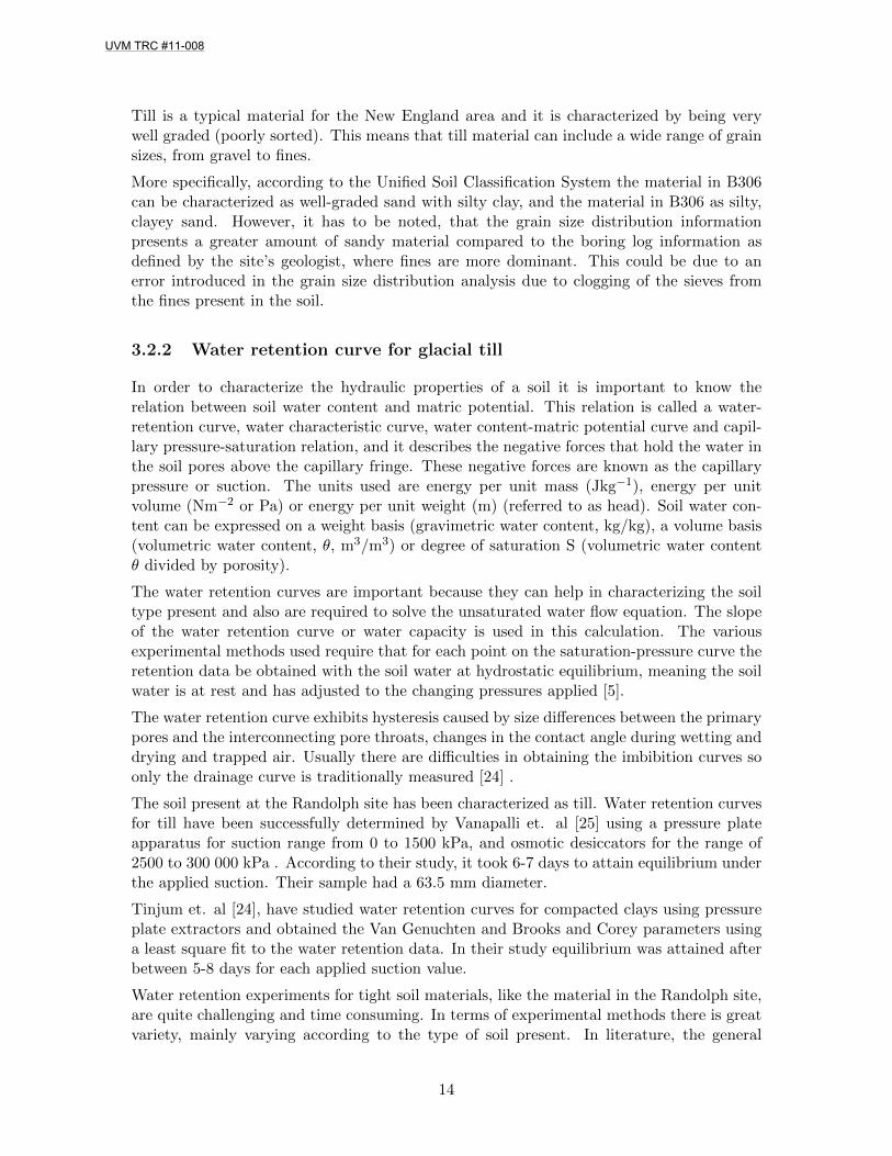
• Method 1: The soil sample is retained by a plastic membrane and placed inside aconfining cell. The cell is filled with water and put under pressure so that the plasticmembrane pushes against the sides of the sample and preferential flow around thesample is prohibited. A porous disc is used as a contact surface between the soilsample and the water pump outlet tube.

• Method 2: No confining cell filled with water is present. The sample is placed insidea conventional pressure cell instead.

• Method 3: Instead of applying air pressure on the top of the sample, the top is leftopen to the atmosphere and negative values of water pressure are used. However, thismethod restricts maximum water pressure to -50 kPa which is the limit of the waterpump.

15

UVM TRC #11-008

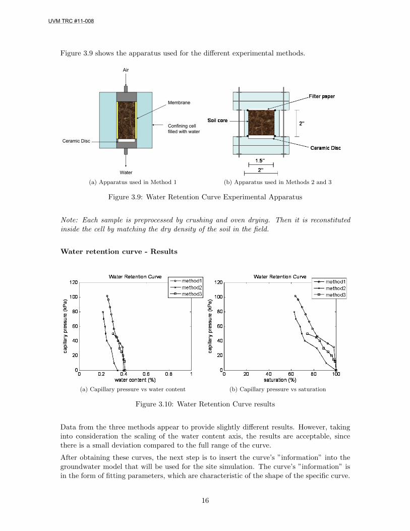
Figure 3.9 shows the apparatus used for the different experimental methods.

(a) Apparatus used in Method 1 (b) Apparatus used in Methods 2 and 3

Figure 3.9: Water Retention Curve Experimental Apparatus

Note: Each sample is preprocessed by crushing and oven drying. Then it is reconstitutedinside the cell by matching the dry density of the soil in the field.

Water retention curve - Results

(a) Capillary pressure vs water content (b) Capillary pressure vs saturation

Figure 3.10: Water Retention Curve results

Data from the three methods appear to provide slightly different results. However, takinginto consideration the scaling of the water content axis, the results are acceptable, sincethere is a small deviation compared to the full range of the curve.

After obtaining these curves, the next step is to insert the curve’s ”information” into thegroundwater model that will be used for the site simulation. The curve’s ”information” isin the form of fitting parameters, which are characteristic of the shape of the specific curve.

16

UVM TRC #11-008

These parameters can be obtained using least square’s fitting software, such as the onlinesoftware SWRC Fit. However, the lack of data points close to residual saturation providederroneous results during the initial trials of the model fitting. In order to overcome thisproblem, another phase of the water-retention experiments needs to be performed. Thisphase will include full saturation of the soil sample and then on-top application of high airpressure, which will allow the water to drain from the bottom. This way a value close tothe residual saturation will be obtained and results from SRWC Fit will be more accurate.This experiment is scheduled to take place in the near future.

3.3 Retention and subsequent evaporation of stormwater

Lack of water accumulation in the drop inlets led to the hypothesis that an amount of watercould be retained by the coarse stone’s surface and then evaporate into the air. In order totest the hypothesis the following experiment was performed.

Experimental Setup

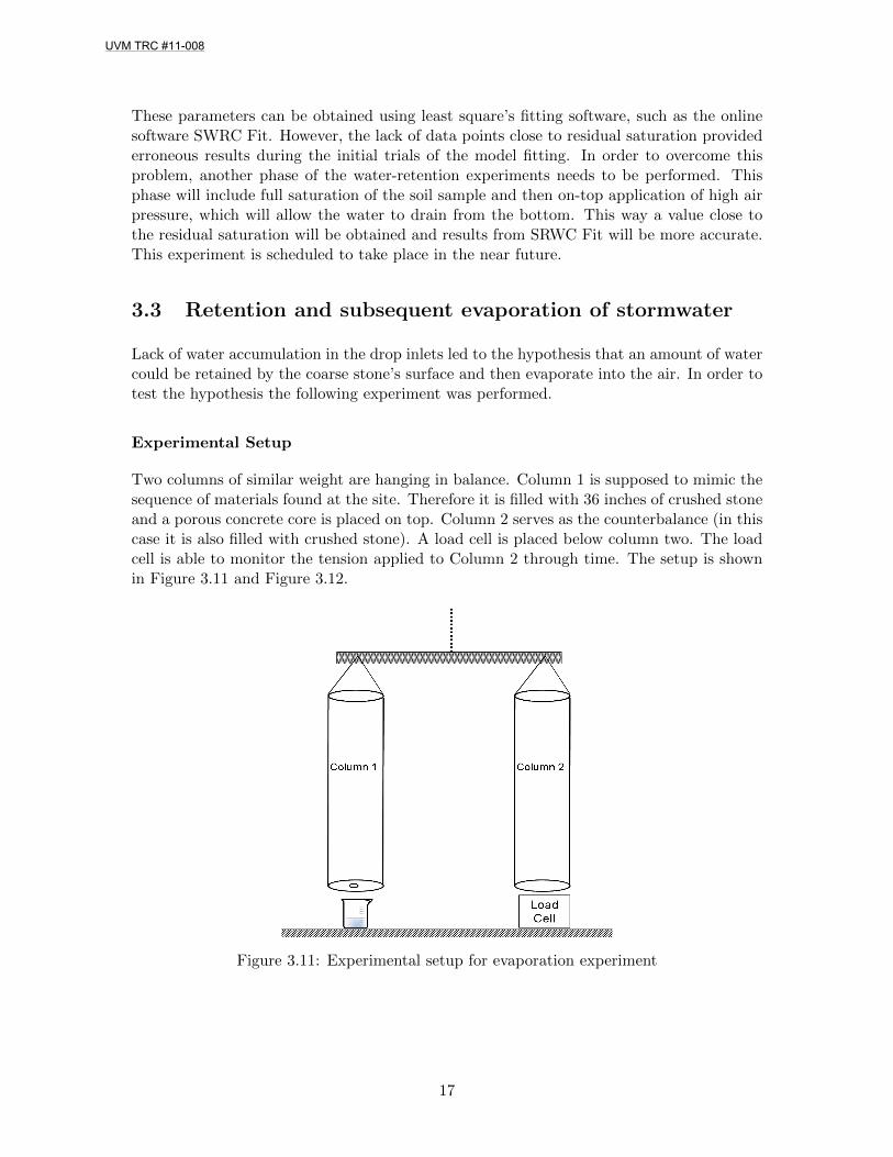
Two columns of similar weight are hanging in balance. Column 1 is supposed to mimic thesequence of materials found at the site. Therefore it is filled with 36 inches of crushed stoneand a porous concrete core is placed on top. Column 2 serves as the counterbalance (in thiscase it is also filled with crushed stone). A load cell is placed below column two. The loadcell is able to monitor the tension applied to Column 2 through time. The setup is shownin Figure 3.11 and Figure 3.12.

Figure 3.11: Experimental setup for evaporation experiment

17

UVM TRC #11-008

(a) Column 1 (b) Column 2 (c) Load cell

Figure 3.12: Detail of Experimental setup

Experimental method

In the first part of the experiment a known amount of water is added as rainfall on top ofColumn 1 causing the balance to shift. Column 1 is left to drain excess water not retainedon the crushed stone through a small opening in the bottom. By knowing the amount ofwater that was added from the top as rainfall and the amount that drained from the bottom,the water withheld by the crushed stone can be calculated. Once water stops draining fromthe column, a rubber plug is used to seal the opening. Water is then left to evaporate.

As the balance shifts with the addition, drainage or evaporation of water, the load cell isable to record all the pressure changes. The amount of evaporation can be then measuredas the difference between two adjacent sequential measurements.

So far 3 tests have been performed.

• Test 1: Column 1 contained only crushed stone. The bottom of Column 1 was opento the atmosphere.

• Test 2: A core of porous concrete was added on top of the crushed stone in column1. The bottom of Column 1 was open to the atmosphere.

• Test 3: Similar to Test 2. The bottom of Column 1 was sealed using a plug.

• Test 4: Similar to Test 2. The bottom of Column 1 was open to the atmosphere.

Results

It should be noted that the different time durations between the tests was mainly due totechnical difficulties and user mistakes while getting acquainted with the equipment. Inaddition, for the same reason, data from the computer in Test 2 were partially scaled sothat the ending point of the computer data would match the starting point of the data fromthe load cell display. This was a safe assumption though, since it was known that thesetwo measurements were taken on the same day and, considering the low evaporation ratesobserved from the other tests at this stage, the deviation should be minimal.

18

UVM TRC #11-008

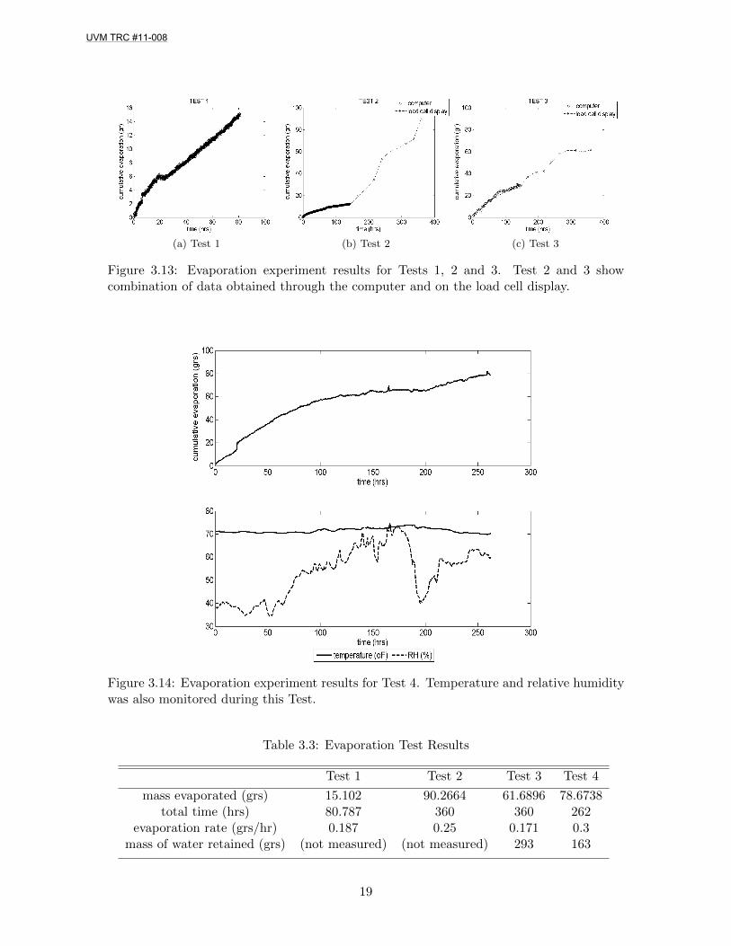
(a) Test 1 (b) Test 2 (c) Test 3

Figure 3.13: Evaporation experiment results for Tests 1, 2 and 3. Test 2 and 3 showcombination of data obtained through the computer and on the load cell display.

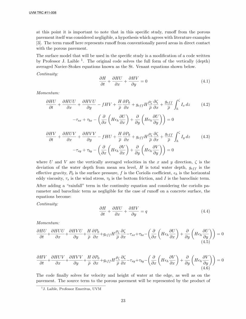
Figure 3.14: Evaporation experiment results for Test 4. Temperature and relative humiditywas also monitored during this Test.

Table 3.3: Evaporation Test Results

Test 1 Test 2 Test 3 Test 4

mass evaporated (grs) 15.102 90.2664 61.6896 78.6738total time (hrs) 80.787 360 360 262

evaporation rate (grs/hr) 0.187 0.25 0.171 0.3mass of water retained (grs) (not measured) (not measured) 293 163

19

UVM TRC #11-008

Experimental results show that there is a significant amount of water retention and evapo-ration inside the coarse stone subbase. However, it does not fully explain the lack of wateraccumulation in the drop inlets.

20

UVM TRC #11-008

Chapter 4

Mathematical Model

The challenge with constructing a mathematical model for a porous concrete system, suchas the one in Randolph, lies in the fact that the physical system is composed of hydrody-namically different interconnected pieces due to the variety of physical processes that takeplace. These processes include:

• surface recharge from rainfall

• runoff from the porous pavement or surrounding conventionally paved areas

• vertical flow into the porous concrete and crushed stone

• potential storage of water inside the crushed stone excavated area

• evaporation

• flow towards the underdrains

• and infiltration into the subsurface.

Therefore the mathematical model that will be used to simulate a porous concrete sitemust not only account for all these processes independently, but also take into account theinterconnection of the different pieces.

21

UVM TRC #11-008

Figure 4.1: Physical processes taking place in a porous concrete system

Due to the complexity of the problem, two different modeling approaches were used.

• First modeling approach: A surface-water model is used to simulate runoff fromconventionally paved areas that at the edges could potentially act as recharge into theporous concrete slab. A groundwater model (VTC) is used to simuate flow throughthe porous concrete to the coarse stone subbase, and finally to the subgrade soil.

Challenge: In this specific modeling approach, there is an extra modelling challengedue to the existence of underdrains inside the coarse stone subbase, which dictatethe flow. A ’correct’ boundary condition is required. Also, the coarse stone materialis not a conventional ’porous media’ since the term containing capillary pressure isnot valid, therefore there is a significant error in the results that the classical porousmedium equations provide.

• Second modeling approach: A surface-water model is used to simulate runoff fromconventionally paved areas that could potentially act as recharge into the porous con-crete slab. Flow through the porous concrete and the coarse stone subbase is simulatedthrough a mass balance model. The surface-water model is also used to simulate flowtowards the underdrains at the bottom of the subbase. Finally a groundwater model(VTC) is used to simulate flow from the subbase to the subgrade soil.

Challenge: There is a high degree of complexity in connecting the three differenetcodes, some of which are written in fortran and others in matlab.

In the following sections the different models are summarized.

4.1 Runoff on pavement module

The runoff component in a porous pavement system is very important since at its perimeterit can add an extra recharge term to the porous pavement. In order to avoid any confusion,

22

UVM TRC #11-008

at this point it is important to note that in this specific study, runoff from the porouspavement itself was considered negligible, a hypothesis which agrees with literature examples[3]. The term runoff here represents runoff from conventionally paved areas in direct contactwith the porous pavement.

The surface model that will be used in the specific study is a modification of a code writtenby Professor J. Laible 1. The original code solves the full form of the vertically (depth)averaged Navier-Stokes equations known as the St. Venant equations shown below.

Continuity:∂H

∂t+∂HU

∂x+∂HV

∂y= 0 (4.1)

Momentum:

∂HU

∂t+∂HUU

∂x+∂HV U

∂y− fHV +

H

ρ

∂P0

∂x+ geffH

ρζρ

∂ζ

∂x+geffρ

∫ ζ

hIx dz (4.2)

−τsx + τbx −(∂

∂x

(Hεh

∂U

∂x

)+

∂

∂y

(Hεh

∂U

∂y

))= 0

∂HV

∂t+∂HUV

∂x+∂HV V

∂y− fHU +

H

ρ

∂P0

∂x+ geffH

ρζρ

∂ζ

∂x+geffρ

∫ ζ

hIy dz (4.3)

−τsy + τby −(∂

∂x

(Hεh

∂V

∂x

)+

∂

∂y

(Hεh

∂V

∂y

))= 0

where U and V are the vertically averaged velocities in the x and y direction, ζ is thedeviation of the water depth from mean sea level, H is total water depth, geff is theeffective gravity, P0 is the surface pressure, f is the Coriolis coefficient, εh is the horizontaleddy viscosity, τs is the wind stress, τb is the bottom friction, and I is the baroclinic term.

After adding a “rainfall” term in the continuity equation and considering the coriolis pa-rameter and baroclinic term as negligible for the case of runoff on a concrete surface, theequations become:

Continuity:∂H

∂t+∂HU

∂x+∂HV

∂y= q (4.4)

Momentum:

∂HU

∂t+∂HUU

∂x+∂HV U

∂y+H

ρ

∂P0

∂x+geffH

ρζρ

∂ζ

∂x−τsx+τbx−

(∂

∂x

(Hεh

∂U

∂x

)+

∂

∂y

(Hεh

∂U

∂y

))= 0

(4.5)

∂HV

∂t+∂HUV

∂x+∂HV V

∂y+H

ρ

∂P0

∂x+geffH

ρζρ

∂ζ

∂x−τsy+τby−

(∂

∂x

(Hεh

∂V

∂x

)+

∂

∂y

(Hεh

∂V

∂y

))= 0

(4.6)

The code finally solves for velocity and height of water at the edge, as well as on thepavement. The source term to the porous pavement will be represented by the product of

1J. Laible, Professor Emeritus, UVM

23

UVM TRC #11-008

the fluid water thickness times the normal velocity at the boundary of the porous concretepavement and the conventional pavement.

One of the challenges in using a surface water model, which is typically used to simulateflow patterns in large water bodies such as oceans or lakes, to simulate runoff on a pavementsurface, is the fact that friction is now an important component. This means that frictioncoefficients in the model needed to be altered in order to provide meaningful results. Inaddition, the model requires a value of the initial height of water on the pavement that, forthe purposes of this simulation, was kept to values on the order of a millimeter. Finally,the main modification in the existing code involved the boundary condition that should beused to simulate flow over the edge of the pavement. The various boundary conditions thatwere tested are the following:

• u = 0. Velocity is equal to 0.

• z = 0. The height of water is equal to 0.

• dzdx = 0. The slope of water surface is equal to 0.

• z=aV2n. From Bernoulli’s law, the elevation head (or height of water in this case)is

equal to the velocity head, where a is a calibration parameter and Vn the velocity ver-tical to the boundary. This boundary condition proved to provide the most meaningfulresults and was used in the majority of the simulations.

4.1.1 Example

In the following example a rainfall event of 1 in/hr on a 50m X 60m domain with slopeof 0.1 % is simulated. The simulated period for this example was kept to 5 minutes. Theboundary condition used was no flow for the perimeter of the domain with the exception ofthe downslope side, where the z=aV2

n boundary condition was used. a = 0.001

Results

(a) Location of “report” nodes (b) Velocity and height of water at “report” nodes

Figure 4.2: Results - Part 1

24

UVM TRC #11-008

(a) Peak surface showing maximum water level response (b) Direction and magnitude flux

Figure 4.3: Results - Part 2

4.2 VTC Module

The groundwater model that will be used in this study is called the Vermont Variably-Saturated Transport Code (VTC). It is a three-dimensional groundwater flow and contami-nant transport model that uses a set of partial differential equations to represent saturatedand unsaturated subsurface flow as well as contaminant transport. The equations are solvedusing finite element and finite differences methods. More specifically, the domain of interestis discretized in horizontal layers and a finite element method is used within each layerallowing the representation of an irregular domain. The layers are then connected verticallyusing a finite difference approximation.

To represent saturated groundwater flow as a function of hydraulic head h the followingequation can be used:

∂

∂x

(Kxx

∂h

∂x

)+

∂

∂y

(Kyy

∂h

∂y

)+

∂

∂z

(Kzz

∂h

∂z

)+ Ss

∂h

∂t− q = 0 (4.7)

And for unsaturated groundwater flow:

∂

∂x

(Kxx

∂h

∂x

)+

∂

∂y

(Kyy

∂h

∂y

)+

∂

∂z

(Kzz

∂h

∂z

)+∂θw∂t

− q = 0 (4.8)

where K is the hydraulic conductivity which in the case of unsaturated flow is a functionof the water content θw. The variable Ss is the specific storage and q is the flux enteringthe groundwater system.

VTC uses an iteration scheme to solve the non-linear equations of unsaturated groundwaterflow, during which relative permeability values are being updated using the Van Genuchtenmodel. The iteration scheme stops when a user-specified convergence criterion is reached.Parameters needed for the Van Genuchten model can be provided experimentally throughthe definition of the water retention curve. Upon successful execution of the code the useris able to plot the solution in the form of a contoured surface or 3-D graph via the Argus

25

UVM TRC #11-008

interface. The VTC graphical user interface (GUI) is written in Fortran. The code has beensuccessfully validated by previous researchers but use for the specific application requiredfurther modifications in the code. At this point the code is able to compute difference insaturation values and plot their contour graph.

As mentioned previously, VTC will be used to either simulate flow through the whole system(porous concrete, coarse stone and subgrade soil) or just the subgrade soil, according to themodeling approach that will provide the most accurate results. In the following example,VTC was used as part of the first modeling approach, meaning to simulate flow throughthe whole system.

4.2.1 Example

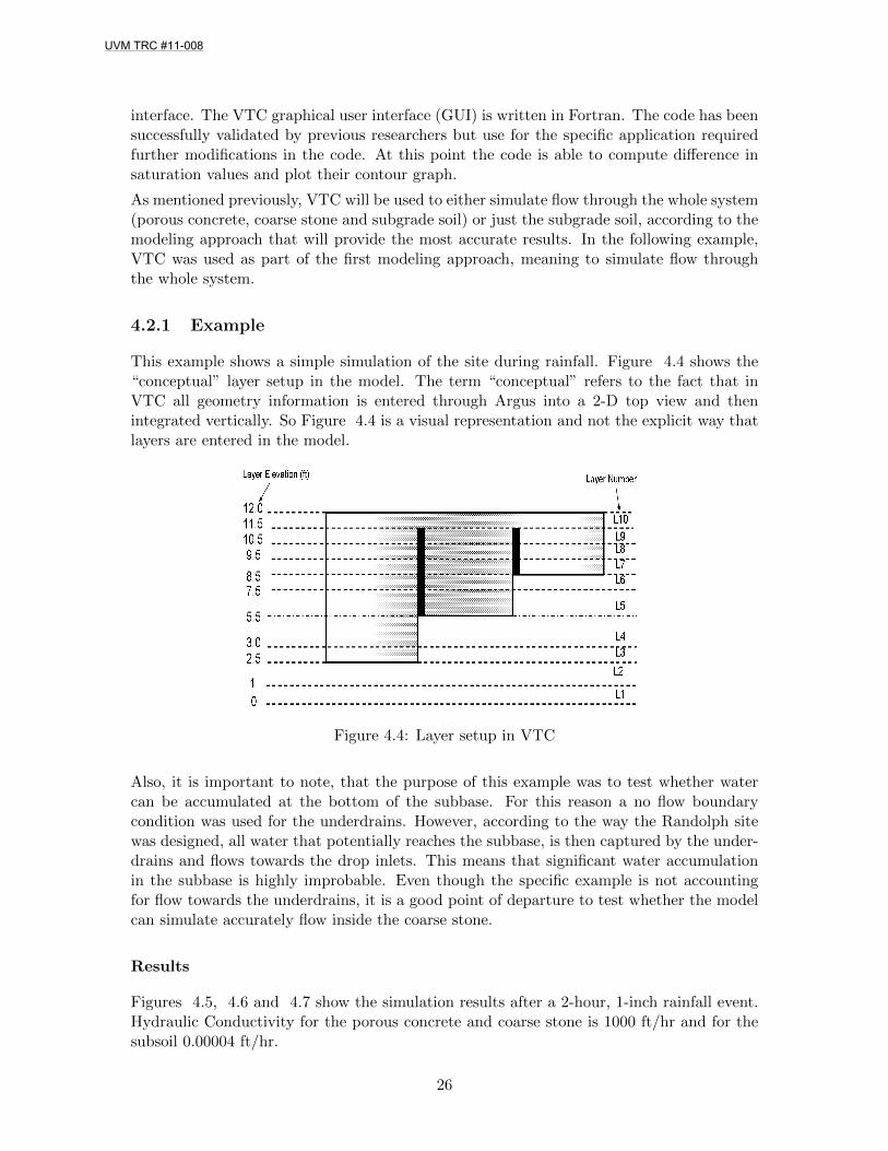
This example shows a simple simulation of the site during rainfall. Figure 4.4 shows the“conceptual” layer setup in the model. The term “conceptual” refers to the fact that inVTC all geometry information is entered through Argus into a 2-D top view and thenintegrated vertically. So Figure 4.4 is a visual representation and not the explicit way thatlayers are entered in the model.

Figure 4.4: Layer setup in VTC

Also, it is important to note, that the purpose of this example was to test whether watercan be accumulated at the bottom of the subbase. For this reason a no flow boundarycondition was used for the underdrains. However, according to the way the Randolph sitewas designed, all water that potentially reaches the subbase, is then captured by the under-drains and flows towards the drop inlets. This means that significant water accumulationin the subbase is highly improbable. Even though the specific example is not accountingfor flow towards the underdrains, it is a good point of departure to test whether the modelcan simulate accurately flow inside the coarse stone.

Results

Figures 4.5, 4.6 and 4.7 show the simulation results after a 2-hour, 1-inch rainfall event.Hydraulic Conductivity for the porous concrete and coarse stone is 1000 ft/hr and for thesubsoil 0.00004 ft/hr.

26

UVM TRC #11-008

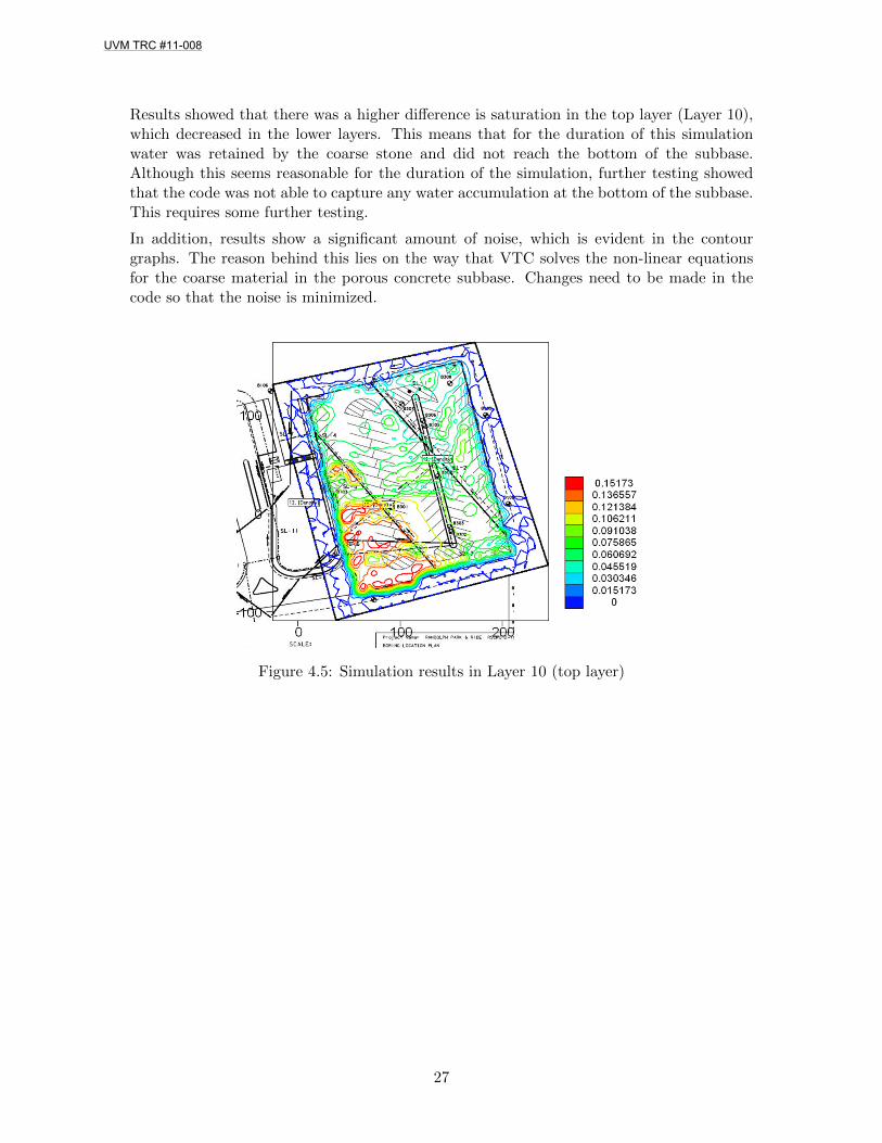
Results showed that there was a higher difference is saturation in the top layer (Layer 10),which decreased in the lower layers. This means that for the duration of this simulationwater was retained by the coarse stone and did not reach the bottom of the subbase.Although this seems reasonable for the duration of the simulation, further testing showedthat the code was not able to capture any water accumulation at the bottom of the subbase.This requires some further testing.

In addition, results show a significant amount of noise, which is evident in the contourgraphs. The reason behind this lies on the way that VTC solves the non-linear equationsfor the coarse material in the porous concrete subbase. Changes need to be made in thecode so that the noise is minimized.

Figure 4.5: Simulation results in Layer 10 (top layer)

27

UVM TRC #11-008

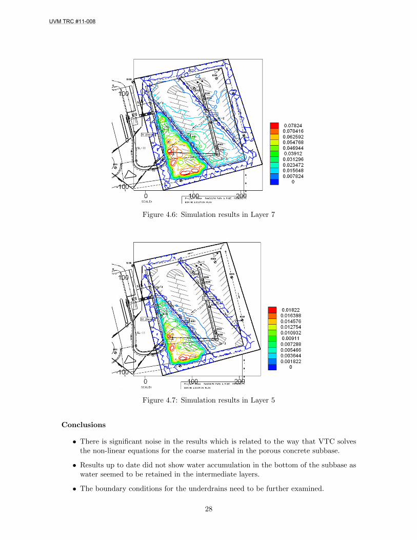
Figure 4.6: Simulation results in Layer 7

Figure 4.7: Simulation results in Layer 5

Conclusions

• There is significant noise in the results which is related to the way that VTC solvesthe non-linear equations for the coarse material in the porous concrete subbase.

• Results up to date did not show water accumulation in the bottom of the subbase aswater seemed to be retained in the intermediate layers.

• The boundary conditions for the underdrains need to be further examined.

28

UVM TRC #11-008

Taking the above into consideration the code needs to be further modified in order torepresent the system more accurately.

4.3 Retention and evaporation of water in the gravel

For the purposes of this study and due to the lack of existing equations found in theliterature, a separate piece of code is currently being developed to describe flow throughthe coarse stone. In the derivation of the appropriate equations the point of departureis the definition of the mass balance equations for the liquid and gas phases. Then theequations describing water in the gas phase, air in the gas phase, air in the liquid phase andwater in the liquid phase are specified. An evaporation term is used to define the amountof water leaving the system. Additional terms for velocity and porosity are present. Aftersimplifying assumptions equation 4.9 is derived:

∫ t

b

∂sl

∂tdz +

∫ t

b

∂slvlz∂z

dz +

∫ t

b

qvs

ρlεdz = 0 (4.9)

where the limits b and t are the bottom and the top of the crushed stone, sl is the liquidwater saturation, vz is the vertical velocity of the water and qvs is the evaporation flux.

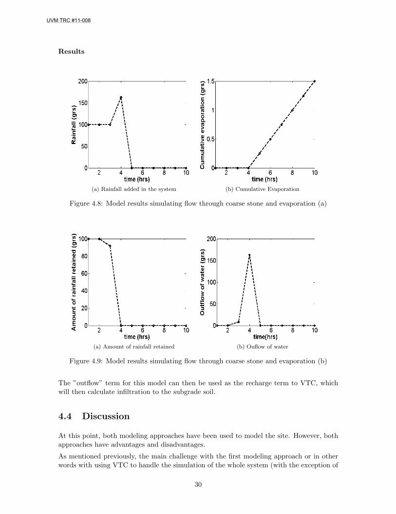
At this point an initial attempt at coding the equations has been performed but the codeneeds to be further enhanced and tested. In this work a simple mass balance code was usedin order to simulate flow through the coarse stone and subsequent evaporation. The inputinto this code is rainfall (in incremental steps), the percentage of water that can be retainedby the coarse stone (as defined in the lab), and the evaporation rate (also defined in thelab). Output is the outflow which is defined as:

Ouflow = Rainfall - Evaporation - Amount of water retained by the stone

4.3.1 Example

In this example:

• Rainfall is added sequentially for the first 4 hours and then it stops.

• Evaporation starts when rainfall has ceased and is equal to 0.171 grs/hr.

• Amount of rainfall retained is 63 % of the original amount of rainfall. After themaximum amount of rainfall is retained any additional rainfall becomes outflow.

29

UVM TRC #11-008

Results

(a) Rainfall added in the system (b) Cumulative Evaporation

Figure 4.8: Model results simulating flow through coarse stone and evaporation (a)

(a) Amount of rainfall retained (b) Ouflow of water

Figure 4.9: Model results simulating flow through coarse stone and evaporation (b)

The ”outflow” term for this model can then be used as the recharge term to VTC, whichwill then calculate infiltration to the subgrade soil.

4.4 Discussion

At this point, both modeling approaches have been used to model the site. However, bothapproaches have advantages and disadvantages.

As mentioned previously, the main challenge with the first modeling approach or in otherwords with using VTC to handle the simulation of the whole system (with the exception of

30

UVM TRC #11-008

runoff), lies in the fact that significant changes are required to the computer code in orderto simulate the coarse stone material. These are changes in the equations used, addition ofan evaporation term (which has been incorporated into the code with questionable success)and perhaps changes in the numerical methods that VTC uses to solve these equations.

Regarding the second modeling approach, where all the different model pieces will be used,the main challenge lies on the way that the pieces will be connected. Connection of matlabwith fortran codes is plausible using matlab MEX files and has been tried successfully bythe authors of this research. However, this also introduces extra mini challenges such asmaking sure that the same time step is used for all different codes, and also technical codeissues.

Taking the above into consideration, it becomes evident that although all the differentpieces that will compose the final mathematical model are present at this point, more timeis required in order two evaluate the two modeling approaches and overcome the variousdifficulties.

31

UVM TRC #11-008

Chapter 5

The Field Experiment

5.1 Reason behind the experiment

Although the Randolph site is equipped with numerous monitoring wells and drain inlets,its complicated design in combination with various equipment malfunctions made on-sitegroundwater level monitoring a challenging task.

According to the site’s design, as soon as water enters the porous concrete slab, and takinginto consideration that the subsoil is composed of dense till deposits, water should gatherin the drop inlets. However, water level data in the drop inlets did not respond as expected.Initial observations could have somehow been skewed by the malfunction of the equipmentas mentioned previously. However, even visual observations verified the assumption thatthe water level gathered inside the inlets did not sum up to the amount of water that wasexpected.

A possible explanation for this issue, except possible construction errors, is the retention ofwater in the coarse stone reservoir and subsequent evaporation.

In order to finally come up with a solid theory of ”where the water is going” Vtrans incollaboration with UVM decided to run a field experiment where a controlled release ofwater would take place on site. Salt would also be added in the water as a tracer.

5.2 The day of the experiment

On August 23rd a crew composed of members of Vtrans, UVM and the local Montpelier firedepartment gathered on site at Randolph Park and Ride for the controlled water release.Around 9.00 am background conductivity and initial water level measurements took place.

The water release took place in three separate events. The first water release took placeat 10.55, the second at 12:45 and the third at 13:50. The release took place on the upperportion of the lot (A3) using the hose and not a sprinkler as was initially suggested mostlydue to time constrains. During the experiment water samples were collected from keylocations around the site.

The following sections present and discuss the data acquired.

32

UVM TRC #11-008

5.3 Results

5.3.1 Water Levels

The following graphs present the water level response in the drop inlets during the threewater release events. In the graphs time 0 refers to August 23rd, 9.04 am. and the threedots indicate the onset of the three separate water release events.

Figure 5.1 shows that both upstream and downstream locations in SP1 respond to theevents in a similar way. The onset of each water release event is accompanied with a slightincrease in water level followed by a slight drop. However, a comparison of the maximumwater level value (1192 ft) to the height of the weir in that location (1194.5 ft) shows thatthe weir was not exceeded.

In SP2, as shown in Figure 5.2, the upstream location responds in a similar manner to thedownstream location of SP1. Actually, the water levels are almost identical which verifiesthe interconnectivity of the two locations through a drain according to the site plans. Thedownstream location is slightly increasing through time. Once again, in the upstreamlocation of SP2 the maximum water level value (1189.5 ft) is still lower than the height ofthe weir (1191.5 ft).

Figure 5.3 shows that there is a water level increase in the upstream location of SP3 whereasthe downstream location is rather unaffected until the third water release event (third dot)when the weir was exceeded. This observation was also visually verified on site.

Water levels in the 200 series wells, as shown in Figure 5.4 and Figure 5.5 do not seem tobe affected by the water release events, with the exception of B203 and B207 where thereis a slight decrease in water level. More specifically in B203 there is a sudden drop in waterlevel after the third event, whereas B207 presents a smoother water level decline.

The 300 series wells showed more clear response to the water release as shown in Figure 5.6and Figure 5.7. However the response was quite surprising. Instead of an increase in waterlevels as it would be expected the specific locations show a significant decline in head whichstarts as soon as the first event takes place. We can see that the phenomenon is obviousin all locations with the exception of well B301 which is the furthest away from the waterrelease location. The drop in head reaches a maximum of almost 4 ft which is a tremendousresponse for the time frame over which it occurred.

Inverse water level response has been previously noted in literature but only for pumpingtests where water is extracted from the aquifer. The phenomenon is known as the Noord-bergum effect 1 and is usually observed in confined and clayey aquifers. The range of inversewater level response found in literature, related to the Noordbergum effect is approximately0.05 ft [20] to 0.2 and 0.3 ft [20], [21]. Further research is required in order to present asolid explanation of the paradox water level response during the field experiment.

1More information on the Noordbergum effect can be found in Appendix D

33

UVM TRC #11-008

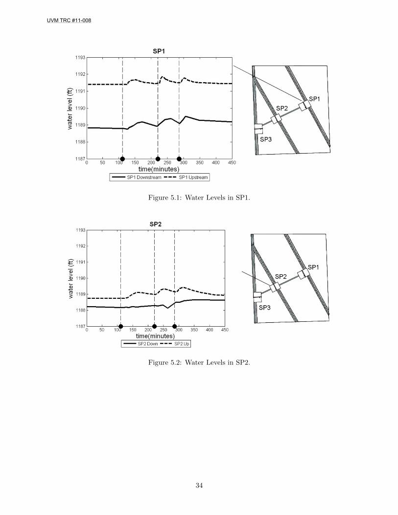
Figure 5.1: Water Levels in SP1.

Figure 5.2: Water Levels in SP2.

34

UVM TRC #11-008

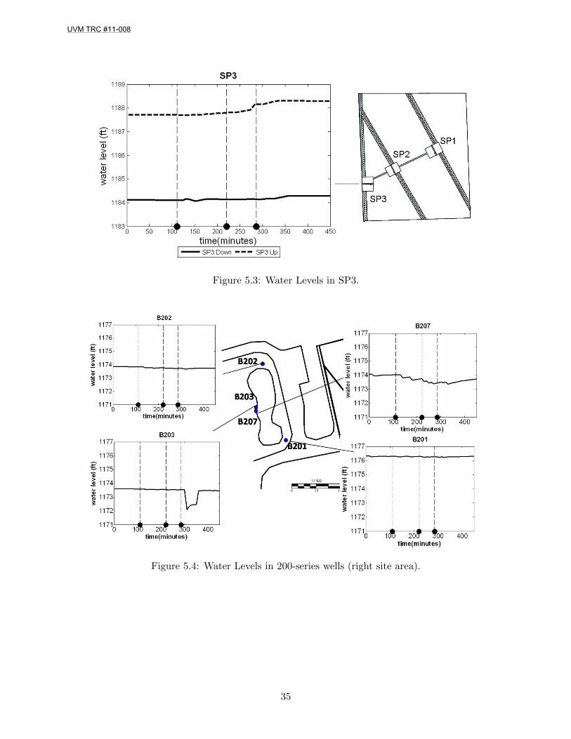
Figure 5.3: Water Levels in SP3.

Figure 5.4: Water Levels in 200-series wells (right site area).

35

UVM TRC #11-008

Figure 5.5: Water Levels in 200-series wells (left site area).

Figure 5.6: Water Levels in 300-series wells (part a).

36

UVM TRC #11-008

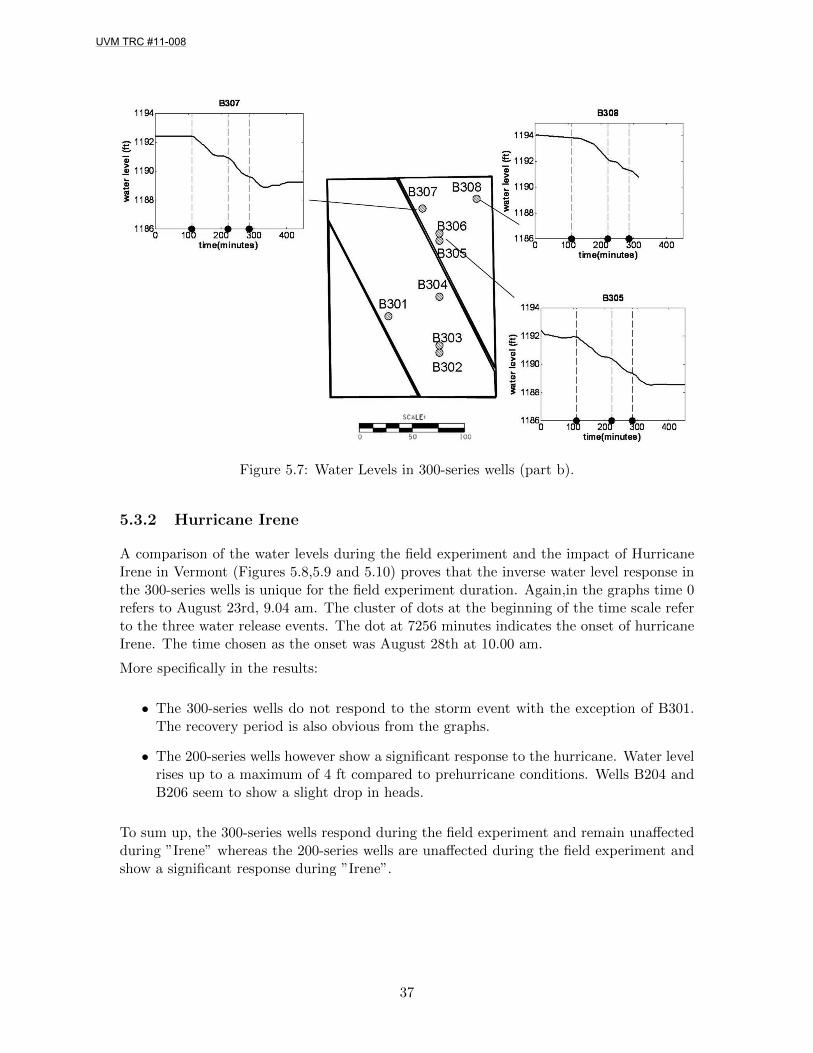
Figure 5.7: Water Levels in 300-series wells (part b).

5.3.2 Hurricane Irene

A comparison of the water levels during the field experiment and the impact of HurricaneIrene in Vermont (Figures 5.8,5.9 and 5.10) proves that the inverse water level response inthe 300-series wells is unique for the field experiment duration. Again,in the graphs time 0refers to August 23rd, 9.04 am. The cluster of dots at the beginning of the time scale referto the three water release events. The dot at 7256 minutes indicates the onset of hurricaneIrene. The time chosen as the onset was August 28th at 10.00 am.

More specifically in the results:

• The 300-series wells do not respond to the storm event with the exception of B301.The recovery period is also obvious from the graphs.

• The 200-series wells however show a significant response to the hurricane. Water levelrises up to a maximum of 4 ft compared to prehurricane conditions. Wells B204 andB206 seem to show a slight drop in heads.

To sum up, the 300-series wells respond during the field experiment and remain unaffectedduring ”Irene” whereas the 200-series wells are unaffected during the field experiment andshow a significant response during ”Irene”.

37

UVM TRC #11-008

Figure 5.8: Water Levels in 300-series wells (part a) - Irene response.

Figure 5.9: Water Levels in 300-series wells (part b) - Irene response.

38

UVM TRC #11-008

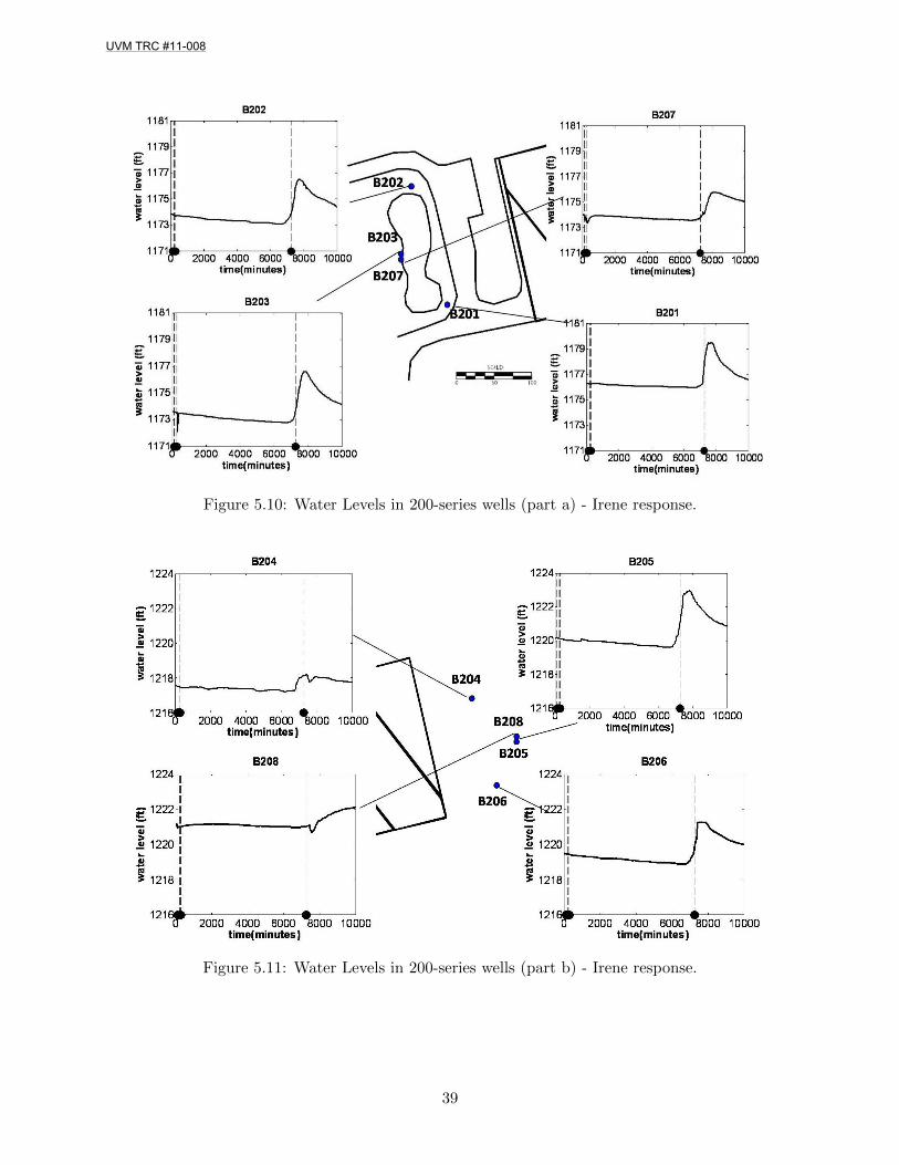
Figure 5.10: Water Levels in 200-series wells (part a) - Irene response.

Figure 5.11: Water Levels in 200-series wells (part b) - Irene response.

39

UVM TRC #11-008

5.3.3 Conductivity Measurements

In addition to the water level monitoring, conductivity measurements were also performedin the various monitoring locations. At first look the data show spiking. However, it mustbe noted that due to time constrains the conductivity measurements were performed quicklyso the spiking could be due to the fact that the conductivity meter has not reached a stablevalue. Also, a different meter was used for the very first measurement compared to the restof the measurements so that might explain the initial sudden response.

Taking the above into consideration, the majority of the wells do not show a clear responsewith the exception of B304 as shown in Figure 5.13 which implies that salt water has reachedthe well.

Figure 5.15 shows that conductivity for SP1 presents a similar pattern to the water levelresponse. In other words saltwater enters both upstream and downstream locations quickly.

The upstream location for SP2 (Figure 5.16) shows a clear increase in conductivity. Thedownstream location shows some peaks which imply salt migration to that area.

In SP3 upstream (Figure 5.17) we see that there is a gradual increase in the concentration,which agrees with the rise in water level. The downstream location presents an increase inconcentration around 320 minutes which is the time that the weir was exceeded.

Figure 5.12: Conductivity measurements in 200-series wells (right side).

40

UVM TRC #11-008

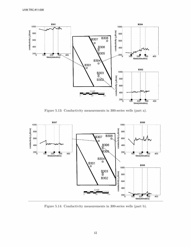
Figure 5.13: Conductivity measurements in 300-series wells (part a).

Figure 5.14: Conductivity measurements in 300-series wells (part b).

41

UVM TRC #11-008

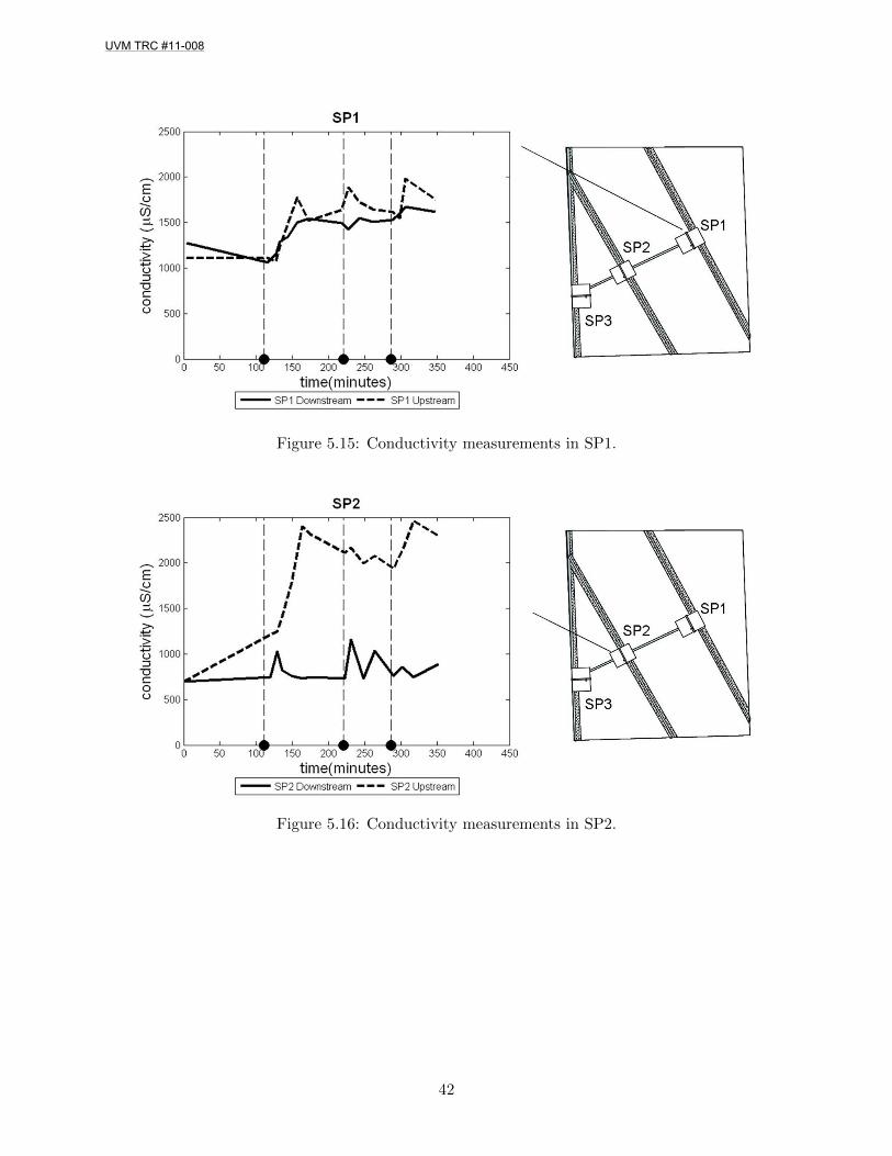
Figure 5.15: Conductivity measurements in SP1.

Figure 5.16: Conductivity measurements in SP2.

42

UVM TRC #11-008

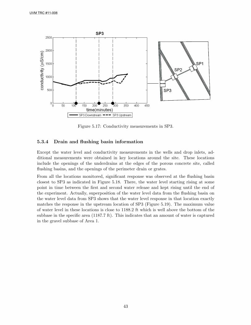
Figure 5.17: Conductivity measurements in SP3.

5.3.4 Drain and flushing basin information

Except the water level and conductivity measurements in the wells and drop inlets, ad-ditional measurements were obtained in key locations around the site. These locationsinclude the openings of the underdrains at the edges of the porous concrete site, calledflushing basins, and the openings of the perimeter drain or grates.

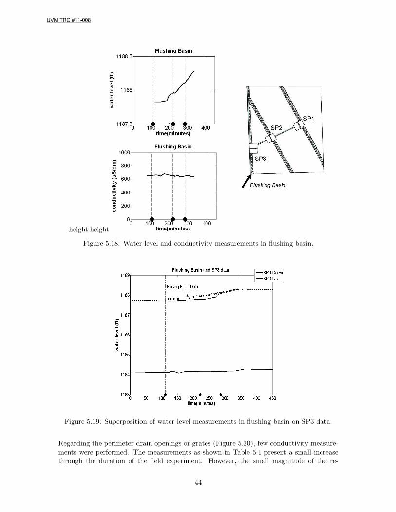
From all the locations monitored, significant response was observed at the flushing basinclosest to SP3 as indicated in Figure 5.18. There, the water level starting rising at somepoint in time between the first and second water release and kept rising until the end ofthe experiment. Actually, superposition of the water level data from the flushing basin onthe water level data from SP3 shows that the water level response in that location exactlymatches the response in the upstream location of SP3 (Figure 5.19). The maximum valueof water level in these locations is close to 1188.2 ft which is well above the bottom of thesubbase in the specific area (1187.7 ft). This indicates that an amount of water is capturedin the gravel subbase of Area 1.

43

UVM TRC #11-008

.height.height

Figure 5.18: Water level and conductivity measurements in flushing basin.

Figure 5.19: Superposition of water level measurements in flushing basin on SP3 data.

Regarding the perimeter drain openings or grates (Figure 5.20), few conductivity measure-ments were performed. The measurements as shown in Table 5.1 present a small increasethrough the duration of the field experiment. However, the small magnitude of the re-

44

UVM TRC #11-008

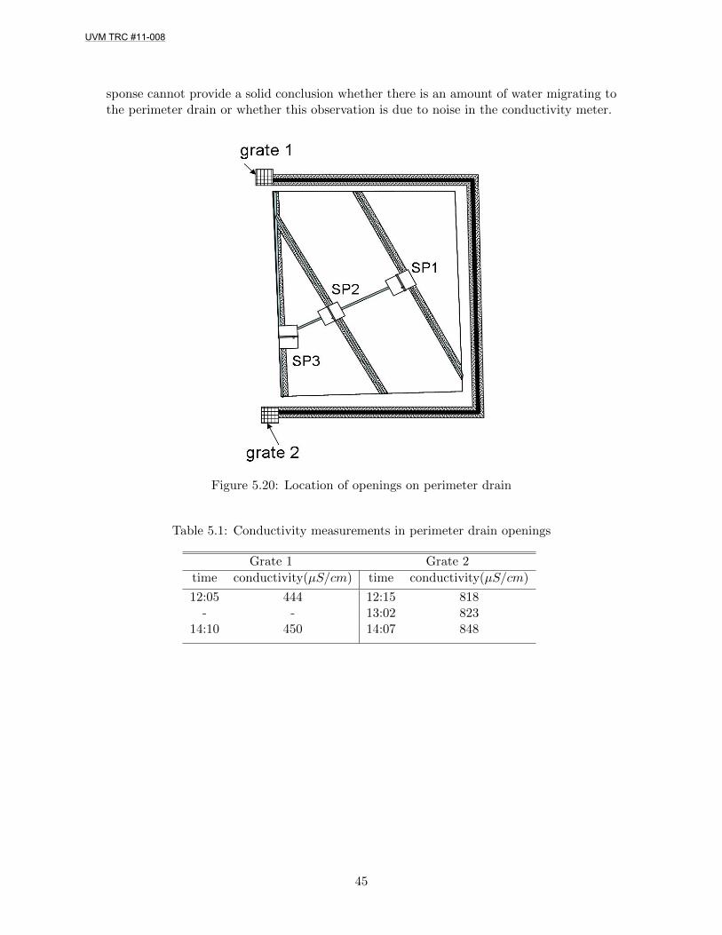
sponse cannot provide a solid conclusion whether there is an amount of water migrating tothe perimeter drain or whether this observation is due to noise in the conductivity meter.

Figure 5.20: Location of openings on perimeter drain

Table 5.1: Conductivity measurements in perimeter drain openings

Grate 1 Grate 2

time conductivity(µS/cm) time conductivity(µS/cm)

12:05 444 12:15 818- - 13:02 823

14:10 450 14:07 848

45

UVM TRC #11-008

5.4 Discussion

Water level measurements in the upstream locations of the three drop inlets show that theweir was not exceeded in SP1 and SP2 but was exceeded in SP3. However, water levelchanges in the downstream locations imply that there is a possibility of leakage through theberm and cutoff wall which are used to separate the three sub-areas of the site. In addition,the height of water in the upstream location of SP3 and the neighbouring flushing basinindicate that there is an amount of water gathered in the gravel subbase of the Area 1.

The 300-series wells shows an inverse water level response during the three water releaseevents. Despite common logic the water levels dropped in response to recharge of the aquifer.The phenomenon shows a tremendous drop close to 4 ft. Although an exact explanation ofthis phenomenon is yet to be determined according to the literature it seems that it mightbe connected to the Noordbergum effect only recorded for pumping tests up to this day.Further research needs to be done.

Another strange phenomenon revealed in the site is the fact that the 300-series wells respondduring the field experiment and remain unaffected during ”Irene” whereas the 200-serieswells are unaffected during the field experiment and show a significant response during”Irene”.

Conductivity measurements in the drop inlets rise in accordance to the water level responseas expected. Although some fluctuation is observed the overall pattern indicates that notsalt is present in the monitoring wells.

Finally, the conductivity data in the perimeter drain do not show clearly whether water iscaptured in the perimeter drain.

46

UVM TRC #11-008

Chapter 6

General Discussion

The Randolph Park and Ride is unique in terms of the instrumentation as well as thelocal geohydrology. The existence of the two artesian wells indicate a high gradient upwardflow, which in combination with the tight geologic subgrade material makes infiltration ofwater into the subsurface very difficult. However, during hurricane Irene and according togroundwater level information for the winter monitoring period of 2010, the groundwaterlevels showed fluctuation. This possibly means that even if water cannot be infiltrated easilyon the area of interest, the local groundwater levels are affected by infiltration in locationsuphill of the porous concrete site.

Laboratory experiments showed that once water infiltrates the porous concrete and coarsestone reservoir, a significant amount is retained by the stone’s surface and then evaporatesinto the atmosphere. However, this combination of phenomena do not justify the lack ofwater accumulation in the drop inlets. The data collected from the controlled water releasefield experiment indicated that there might be some leakage through the cutoff wall andberm, allowing water to move from one “area” to another without exceeding the weir.

Concerning the hypothesis that an amount of water could be leaking towards the perimeterdrain, there are still no solid conclusions. Conductivity measurements in the drain inletsdid not show a clear salt presence in these locations.

In terms of the mathematical model that is used to simulate the site, it is obvious that thereare many challenges, mainly due to the complexity of the problem. Although the variousmodel pieces are present, and provide reasonable results individually, more time is neededin order to compose the final model and to perform a simulation of the whole system. Also,the implementation of the optimization algorithm remains a secondary goal of this research.

The field experiment showed inverse water level response during recharge of the aquifer. Thedata set collected showed clearly the inverse respond from the wells located on the porousconcrete area. The first hypothesis is that the phenomenon observed in the field is a formof the Noordbergum effect. Taking into consideration the rarity of the specific phenomenonand more importantly the rarity of such a well-documented data set, it becomes clear thatthis finding is very significant for the literature. Further research into the phenomenon willprovide better understanding of the field conditions.

47

UVM TRC #11-008

Bibliography

[1] C. T. Andersen, I. D. L. Foster, and C. J. Pratt. The role of urban surfaces (perme-able pavements) in regulating drainage and evaporation: development of a laboratorysimulation experiment. Hydrological Processes 13, 1999.

[2] M. Backstrom. Ground temperature in porous pavement during freezing and thawing.Journal of Transportation Engineering, 2000.

[3] E. Z. Bean, W. F. Hunt, and D. A. Bidelspach. Evaluation of four permeable pavementsites in eastern north carolina for runoff reduction and water quality. Impacts Journalof Irrigation and Drainage Engineering, 2007.

[4] B. O. Brattebo and D. B. Booth. Long-term stormwater quantity and quality perfor-mance of permeable pavement systems. Water Resources, 2004.

[5] J. H. Dane and J. W. Hopmans. Methods of soil analysis. Part 4 - Physical methods,chapter 3, pages 671–700. Number 5. Soil science society of America, Inc., Madison,Wisconsin, USA, 2002.

[6] E. E. Dreelin, L. Fowler, and C. R. Carroll. A test of porous pavements effectivenesson clay soils during natural storm events. Water Research, 2006.

[7] E. A. Fassman and S. Blackbourne. Urban runoff mitigation by a permeable pavementsystem over impermeable soils. Journal of Hydrologic Engineering, 2010.

[8] B. K. Ferguson. Porous Pavements. CRC Press, 2005.

[9] E. Gomez-Ullate, J. R. Bayon, D. Castro, and S. J Coupe. Influence of the geotextileon water retention in pervious pavements. In 11th International Conference on UrbanDrainage.

[10] M. F. Hein and A. K. Schindler. Learning pervious concrete:concrete collaboration ona university campus. Technical report, 2005.

[11] V. Henderson and S. L. Tighe. Pervious concrete performance in field applications andlaboratory testing. Technical report, 2010.

[12] J. L. Hoffman. The Noordbergum Effect. Technical report, New Jersey GeologicalSurvey Technical Memorandum, 1984.

[13] P. A. Hsieh. Poroelasticity simulation of ground-water flow and subsurface deformation.In U.S. Geological Survey Subsidence Interest, pages 5–9, February 14-16 1995.

48

UVM TRC #11-008

[14] W. Robert C. James, W. James, and H. V. Langsdorff. Stormwater management modelfor environmental design of permeable pavement. In Models and Applications to UrbanWater Systems, 2001.

[15] J. Kim and R. R. Parizek. Numerical simulation of the Rhade effect in layered aquifersystems due to groundwater pumping shutoff. Advances in Water Resources, pages627–642, 2005.

[16] T. E. Kunzen. Hydrologic mass balance of pervious concrete pavement with sandysoils. Master’s thesis, University of Central Florida, 2004.

[17] M. Kwiatkowski. Water quality study of a porous concrete infiltration best managementpractice. Master’s thesis, Villanova University, 2004.

[18] G. P. Ong and T. F. Fwa. Analysis and design of vertical-drainage geosynthetic-reinforced porous pavement for roads and car parks. Journal of the Eastern AsiaSociety for Transportation Studies, 2005.

[19] G. F. Pinder and M. A. Celia. Subsurface Hydrology, chapter 1, pages 12–13. Wiley,2006.

[20] L. M. Piper. Analysis of unexpected results of water level study to determine aquiferinterconnection. In Proceedings of the Fifth National Outdoor Action Conference onAquifer Restoration, Ground-Water Monitoring and Geophysical Methods, pages 205–209, Dublin, OH, 1991. National Ground-water association.

[21] J. D. Rodrigues. The Noordbergum effect and characterization of aquitards at the RioMaior mining project. GROUND WATER, 21(2):200–207, March-April 1983.

[22] L. A. Rossman. Stormwater Management Model Users Manual Version 5.0.

[23] W. Schluter and C. Jefferies. Modelling the outflow from a porous pavement. In UrbanWater 4.

[24] J. M. Tinjum, C. H. Benson, and L. R. Blotz. Soil-water characteristic curves forcompacted clays. Journal of Geotecnical engineering, 1997.

[25] S. K. Vanapalli, D. G. Fredlund, and D. E. Pufahl. The relationship between the soil-water characteristic curve and the unsaturated shear strength of a compacted glacialtill. Geotechnical Testing Journal, 19(3):259–268, September 1996.

[26] M. Wanielista, M. Chopra, J. Spence, and C. Ballock. Hydraulic performance assess-ment of pervious concrete pavements for stormwater management credit. Technicalreport, 2007.

49

UVM TRC #11-008

Appendices

50

UVM TRC #11-008

Appendix A

100-series wells

51

UVM TRC #11-008

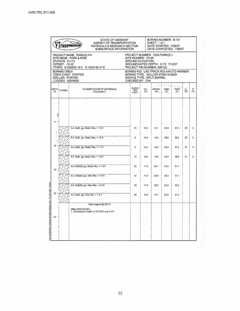
52

UVM TRC #11-008

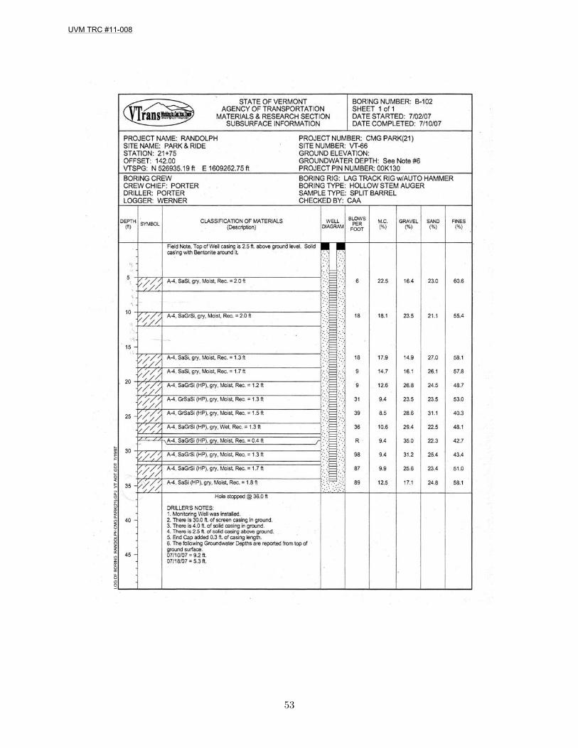
53

UVM TRC #11-008

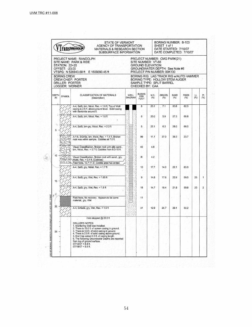
54

UVM TRC #11-008

55

UVM TRC #11-008

56

UVM TRC #11-008

57

UVM TRC #11-008

Appendix B

200-series wells

58

UVM TRC #11-008

59

UVM TRC #11-008

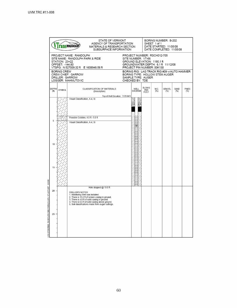
60

UVM TRC #11-008

61

UVM TRC #11-008

62

UVM TRC #11-008

63

UVM TRC #11-008

64

UVM TRC #11-008

65

UVM TRC #11-008

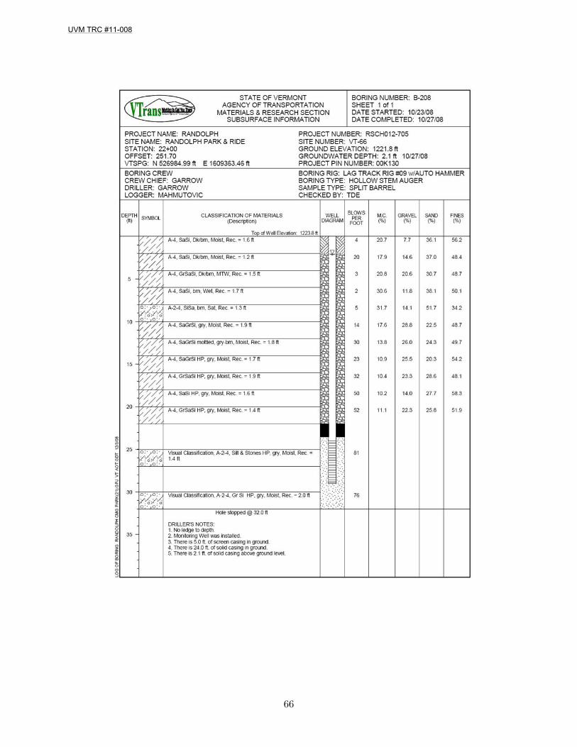
66

UVM TRC #11-008

Appendix C

300-series wells

67

UVM TRC #11-008

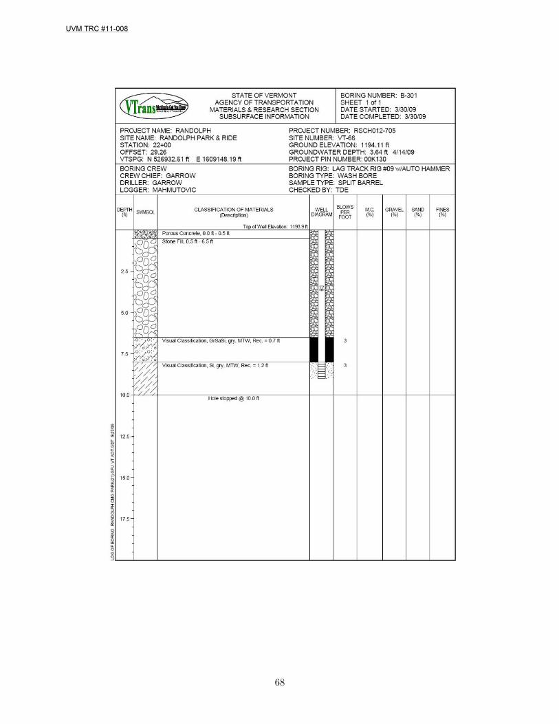
68

UVM TRC #11-008

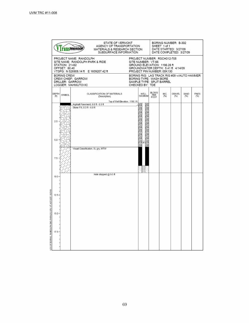
69

UVM TRC #11-008

70

UVM TRC #11-008

71

UVM TRC #11-008

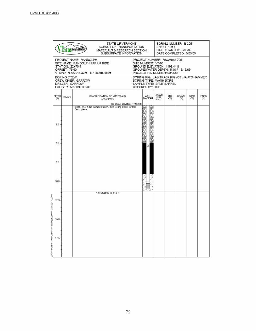
72

UVM TRC #11-008

73

UVM TRC #11-008

74

UVM TRC #11-008

75

UVM TRC #11-008

Appendix D

The Noordbergum effect

The Noordbergum effect, or in other words a reverse (upward) water level response due topumping, is a rare phenomenon that has however been reported in literature as early asthe 1980s. The effect occurs axially symmetrically around pumping wells in aquitards andunpumped aquifers adjacent to pumped aquifers. The rapid head rise at the beginning ofgroundwater pumping is called the Noordbergum effect while the rapid head drops at theend of the pumping is called the Rhade effect. These names derive from the locations wherethe effects were first observed [15].

One of the first observations of the Noordbergum effect was by Jose Delgado Rodrigues [21]in 1983. As part of a project aiming at exploiting the Rio Maior lignite deposits an aquifercharacterization was needed, and therefore pumping tests were performed in the field. Thepumping test showed inverse water level response in several piezometers in distances up to140 m from the pumping well. The author defined the Noordbergum effect as a reversewater level response in aquitards or in aquifers separated from the pumped aquifer byaquitards, during early stages of pumping and recovery tests. The paradoxal behavior ofthe piezometric surface is similar to effects obtained due to three dimensional consolidationand can therefore also be called the Mandel-Cryer effect. In the specific research the authorconsidered that pumping of the upper layer of an aquifer would attract water from the lowerlayer and promote a decrease in volume with a tendency to compression in the lower layer.Since pore water opposes compression of the soil, there would be an increase in pore-waterpressure causing the water levels to rise in the piezometers.

Hoffman [12] presents different definitions of the Noordbergum effect including one forunconfined aquifers. In this case as sediments are dewatered in the aquifer during pumpingan amount of water is retained in the vadose zone. This water has contributed to thehydrostatic force when it was part of the saturated zone but as part of the unsaturated itdoes not. This means that hydrostatic pressure in the saturate zone decreases faster thanthe total pressure and consequently intergranular pressure increases.

A more detailed definition of the Noordbergum effect is provided by Piper [20] in a reportinvestigating a confined sandy aquifer underlain by a clay layer and an unconfined alsosandy aquifer in Maryland. The intergranular pressure at the bottom of the confining layeris equivalent to the weight of the soil and water above it, minus the hydrostatic pressureexerted upward by the confined aquifer. When pumping begins the weight of the soil andwater remain the same since this is a confined aquifer and a decline in the piezometriczone does not cause desaturation but the hydrostatic pressure decreases. This causes the

76

UVM TRC #11-008

intergranular pressure to be greater during pumping. The increase in the intergranularpressure causes the pore water to be squeezed out of the pores and the soil matrix and soilcompression takes place. The reduction in the volume of the compressed layers is the sameas the volume of the water squeezed out.

Finally, the Noordergum effect has been modeled by Hsieh [13]. The model is a finiteelement model which solves the axisymmetric form of the poroelastic equations and analyzesdeformation-induced changes in hydraulic head.

77

UVM TRC #11-008