numerical methods for the vlasov equation

Numerical methods for the Vlasov equation

Eric Sonnendrucker

IRMAUniversite de Strasbourg

project-team CALVIINRIA Nancy Grand Est

September 13, 2011

Eric Sonnendrucker (Univ. Strasbourg) Numerical methods for the Vlasov equation September 13, 2011 1 / 107

Outline

1 Plasma physics

2 ModelsConservation properties of Vlasov-Maxwell systemReduced models

3 Numerical solution of the Vlasov equationIntroductionParticle MethodsPhase space grid-based methods

4 Code validationGeneral considerationsSolution of linearized Vlasov-Poisson


Outline

1 Plasma physics





Plasmas

When a gas is heated to a temperature of more than 104 K electronsleave their orbit around the nucleus to which they belong.

Gas becomes a globally neutral mixture of ions, electrons and neutralswhich is called plasma.

Plasmas are considered in addition to solid, liquid and gas to be thefourth state of matter.

99% of the mass of the universe consists of plasmas.

Many applications: satellite amplifiers, plasma etching inmicro-electronics, X-ray production, TVs, ...., thermonuclear fusion.


Controlled thermonuclear fusion

Magnetic confinement (ITER)

Inertial confinement

laser (LMJ)heavy ions


The ITER project

International project involving European Union, China, India, Japan, SouthKorea, Russia and United States aiming to prove that magnetic fusion isviable source for energy.


Outline

1 Plasma physics





The Vlasov-Maxwell system

∂fs∂t

+ v · ∂fs∂x

+qs

ms(E + v × B) · ∂fs

∂v= 0, (1)

− 1

c2

∂E

∂t+∇× B = µ0 J,

∂B

∂t+∇× E = 0,

∇ · E =ρ

ε0,

∇ · B = 0.

with

ρ(x, t) =∑s

qs

∫fs(x, v, t) dv, J(x, t) =

∑s

qs

∫fs(x, v, t)v dv.


Outline

1 Plasma physics





One species Vlasov-Maxwell system

We consider only one species of particles and set all physical constants to1 for simpler computations. Domain periodic in x and whole space in vResults carry over to general model.

∂f

∂t+ v · ∇x f + (E + v × B) · ∇v f = 0, (2)

−∂E∂t

+∇× B = J, (3)

∂B

∂t+∇× E = 0, (4)

∇ · E = ρ, (5)

∇ · B = 0, (6)

with

ρ(x, t) =

∫f (x, v, t) dv, J(x, t) =

∫f (x, v, t)v dv.


Characteristics of Vlasov equation

The solution of the Vlasov equation can be expressed with help ofcharacteristics which are the solutions of the differential system

dX

dt= V(t), (7)

dV

dt=

q

m(E(X(t), t) + V(t)× B(X(t), t)). (8)

Characteristics are denoted by

(X(t; x, v, s),V(t; x, v, s))

Solution of Vlasov equation then writes

f (x, v, t) = f0(X(0; x, v, t),V(0; x, v)).


Conservative form of Vlasov equation

Vlasov equation can be written in conservative form

∂f

∂t+∇x,v · (Ff ) = 0, (9)

with F = (v,E + v × B)T such that ∇x,v · F = 0.

Conservation of total number of particles∫f (x, v, t) dx dv

follows by integrating in phase space.


First conservation properties

Maximum principle

0 ≤ f (x, v, t) ≤ max(x,v)

(f0(x, v)). (10)

Follows fromf (x, v, t) = f0(X(0; x, v, t),V(0; x, v)).

Conservation of Lp norms

d

dt

(∫(f (x, v, t))p dx dv

)= 0 (11)

Multiply Vlasov eq. by f p−1 and integrate over phase space.


Conservation of phase space volume

For any volume V of phase space∫V

f (x, v, t) dx dv =

∫F−1(V )

f0(y,u) dy du. (12)

Jacobian of flow is equal to one because phase space divergence ofadvection field

(v,E + v × B)T

vanishes.


Conservation of momentum and energy

Momentum conservation

d

dt

[∫vf dxdv +

∫E× B dx

]=

d

dt

[∫J dx +

∫E× B dx

]= 0. (13)

Energy conservation

d

dt

[1

2

∫|v|2f dxdv +

1

2

∫(E 2 + B2) dx

]= 0. (14)


Outline

1 Plasma physics





Vlasov-Poisson model

The one species Vlasov equation reads

∂f

∂t+ v · ∇x f + E · ∇v f = 0. (15)

It is coupled to the Poisson equation

−∆φ = 1− ρ = 1−∫

f (t, x , v) dv , E = −∇φ.

1D Vlasov-Poisson equation first standard model.


Specificities of Tokamaks

Large magnetic field.

Particle trajectories mostly confined along magnetic field lines.

Many instabilities of magnetized plasmas.

Toroidal geometry


The drift-kinetic model (in slab geometry)

Taking the limit of a large magnetic field we get a 4D model(r , θ, φ, v‖)

∂f

∂t+ vD · ∇x f + v‖ · ∇‖f +

q

mE‖ · ∇v f = 0,

with vD = E×BB2 . Poisson’s equation might be replaced by the

quasi-neutrality relation

−∇⊥ · (n0(r)

Bωc∇⊥φ) +

e n0(r)

Te(r)(φ− λ〈φ〉) = n − n0,

〈φ〉 representing the average of the potential over the magnetic fluxlines.

Guiding-center model as a starting point.


The gyrokinetic model

It is a 5D model describing the evolution ofthe guiding center distributionf (r , θ, φ, v‖, µ)

∂f

∂t+ vD · ∇x f + v‖ · ∇‖f +

q

mE‖ · ∇v f = 0,

with vD = −∇J(φ)×BB2 , coupled with the quasi-neutrality equation

−∇⊥ · (n0(r)

Bωc∇⊥φ) +

e n0(r)

Te(r)(φ− λ〈φ〉) =

∫J(f ) dv‖dµ− n0.

The gyroaverage operator J transforms the guiding-center distributiononto the actual particle distribution enabling to take into account thefinite Larmor radius.


Outline

1 Plasma physics





Kelvin-Helmoltz instability in magnetized plasma (1/3)


Numerical simulation of kinetic equations

Difficulties:

defined in phase space (4D, 5D or 6D).Appearance of small scales. Filamentation.

Particle methods: more efficient in high dimensions.

Good qualitative results at relatively low costNumerical noise and slow convergence → difficult to have accurateresults in some situations.

Methods using a grid of phase space:

Huge amount of computations in more than 3 dimensions.No numerical noise, but diffusion.Small scales at some point will not be resolved by the grid.Need to dissipate them for stability. How? Subgrid model?Entropy cannot be conserved for long time simulations

Fourier Transform in velocity space (Eliasson). Replace subgridresolution problem by boundary conditions to evacuate high modes.


Outline

1 Plasma physics





Particle Methods

Particle-In-Cell (PIC) method :

Idea: Follow particle trajectories, use grid field solve.Literature:

Physics (Birdsall-Langdon, Hockney-Eastwood)Mathematical analysis (Neunzert-Wick, Cottet-Raviart, Victory-Allen)

SPH type methods:

Idea: Compute interaction between finite sized macro-particles.Literature: (Bateson-Hewett)


Discretization of the Vlasov equation by a particle method

Particle approximation of the Vlasov equation. Distribution functionis approximated by

fh(x , v , t) =∑k

wkδ(x − xk(t))δ(v − vk(t)).

Deterministic, pseudo-random or Monte-Carlo approximation of f0.

Once particles have been initialized, they are advanced usingdeterministic equations of motion

dxkdt

= vk ,dpk

dt= q(E (xk , t) + vk ∧ B(xk , t)).


Discrete particle motion

Independent of mesh.

Once fields at particle positions are known, equations of motion aregenerally discretized using a Leap-Frog scheme.

xn+1k − xnk

∆t= v

n+ 12

k

vn+ 1

2k − v

n− 12

k

∆t=

q

m(En

k + vnk × Bnk)

Use Boris trick to avoid acceleration by magnetic field

v− = vn− 1

2k +

q

2mEn

v+ − v−

∆t=

q

2m(v+ + v−)× Bn

vn+ 12 = v+

k +q

2mEn


Coupling particles with fields through shape functions

Particle method defines point particles (Dirac masses).

Regularization by convolution with a finite width smoothing kernelgenerally called weighting function.

Splines of different orders on are generally used on structured grids

NGP CIC order 2

P1 Finite Element shape functions on unstructured grids.Generally fields obtained by Poisson or Maxwell field solver firstinterpolated at vertices of meshTruncated Gaussians have also been used by some authors(Jacobs-Hesthaven).


Coupling with the Field solver: The Particle-In-Cell Method

Particle data scattered to surrounding grid pointsto compute charge and current densities usingweight function:

ρi = q∑k

S(xk − xi ), Ji = q∑k

S(xk − xi )vk .

Field solve performed on grid: E(xi ), B(xi ) arecomputed using some grid based field solver.

Fields are computed on particles usinginterpolation e.g. E(xk) =

∑S(xk − xi )E(xi ).


Noise reduction techniques

Statistical noise reduction techniques can be applied:

δf methods. Decompose f = f 0 + δf and use particle approximationonly for perturbation. Decreases noise where δf << f 0.

Ef (Si )) = Ef 0(Si )) + Ef−f 0(Si ))

=

∫Si (x)f 0(x , v) dx dv +

∫Si (x)(f (x , v)− f 0(x , v)) dx dv

First part is known exactly, only second part is approximated bysample and its variance is a lot smaller if δf << f 0.

Very efficient when f stays close to known equilibrium as in sometokamak plasma simulations.


Outline

1 Plasma physics





The model

An abstract form of a kinetic equation reads

∂f

∂t+ a(z, t) · ∇f = 0,

z are the phase space coordinates, a depends non linearly and nonlocally on f , through e.g. the electromagnetic field.

The velocity field a is divergence free so that the equation can also bewritten in conservative form

∂f

∂t+∇ · (f a) = 0.

Mathematically for a given a the non conservative form is a transportequation which can be solved using the characteristics, which are thesolution of the ODE

dZ

dt= a(Z, t).


Operator splitting

Consider e.g. the non relativistic Vlasov-Poisson equation

∂f

∂t+ v · ∇x f +

q

mE · ∇v f = 0.

We decompose the equation into the two following steps.

∂f

∂t+ v · ∇x f = 0, (16)

with v fixed and∂f

∂t+

q

mE(x, t) · ∇v f = 0, (17)

with x fixed.

We solve the two equations successively on one time step. At leastdimension reduction and in our example constant coefficientadvections for reduced equations.


Analysis of splitting error

For constant coefficient differential operators A and B we consider

du

dt= (A + B)u

Formal solution on one time step reads

u(t + ∆t) = e∆t(A+B)u(t).

Split equations read

du

dt= Au,

du

dt= Bu.

with formal solutions on one time step

u(t + ∆t) = e∆tAu(t) et u(t + ∆t) = e∆tBu(t).


Analysis of splitting error

If operators A and B commute split solution

u(t + ∆t) = e∆tBe∆tAu(t)

exact.

This is the case for constant coefficient transport not for generalVlasov.

Alternate solution of A and of B on substeps to get any given order.Negative time advance coefficients starting from third order splitting.

Coefficients are found by equating first terms of Taylor expansion ofexponential.


First order splitting

Successive solution on one time step is first order in time.

e∆t(A+B) = I + ∆t(A + B) +∆t2

2(A + B)2 + O(∆t3),

e∆tBe∆tA = (I + ∆tB +∆t2

2B2 + O(∆t3))(I + ∆tA +

∆t2

2A2 + O(∆t3))

= I + ∆t(A + B)∆t2

2(A2 + B2 + 2BA) + O(∆t3)).

If A and B do not commute we have(A + B)2 = A2 + AB + BA + B2 6= A2 + B2 + 2BA.


Second order splitting

Strang splitting is second order: Solve A on half time step, B on full timestep, again A on half time step.

e∆t(A+B) = I + ∆t(A + B) +∆t2

2(A + B)2 + O(∆t3),

e∆t2Ae∆tBe

∆t2A =(I +

∆t

2A +

∆t2

4A2 + O(∆t3)))(I + ∆tB +

∆t2

2B2

+ O(∆t3))(I +∆t

2A +

∆t2

4A2 + O(∆t3)))

=I + ∆t(A + B) +∆t2

2(A2 + B2 + BA + AB) + O(∆t3).


Development of methods based on phase space grid

The semi-Lagrangian method (generalization of Cheng and Knorrsplitting method).

Vlasov solver based on WENO method (Carrillo-Vecil, Qiu-Chrislieb,Qiu-Shu, Banks-Hittinger).

Discontinuous Galerkin (Qiu-Shu, Gamba-Morrison, Rossmanith-Seal,Crouseilles-Mehrenberger-Vecil)

Conservative flux based methods : (Boris-Book, Fijalkow,Filbet-ES-Bertrand, Crouseilles-Mehrenberger-ES).

Energy conserving Finite Difference (Arakawa).

Fourier in velocity space (Eliasson).


History of semi-Lagrangian schemes for Vlasov

Cheng-Knorr (JCP 1976): splitting method for 1D Vlasov-Poisson.Cubic spline interpolation.

ES-Roche-Bertrand-Ghizzo (JCP 1998): general semi-Lagrangianframework for Vlasov-type equations.

Nakamura-Yabe (CPC 1999): semi-Lagrangian CIP method withHermite interpolation

Filbet-ES-Bertrand (JCP 2001) : semi-Lagrangian PFC method:positive and conservative

N. Besse - ES (JCP 2003) : semi-Lagrangian solver on unstructuredgrids.

V. Grandgirard et al. (JCP 2006): drift-kinetic SL scheme.

Crouseilles-Respaud-ES (CPC 2009): Forward semi-Lagrangian

Crouseilles-Mehrenberger-ES (JCP 2010): Equivalence of point basedand conservative methods for Vlasov-Poisson + new class of filters.

Qiu-Christlieb (JCP 2010): conservative SL WENO schemes.

Qiu-Shu (JCP 2011): DG SL schemes.


Convergence of semi-Lagrangian schemes for Vlasov

Filbet (SINUM 2001): PFC method for Vlasov-Poisson

N. Besse (SINUM 2003): semi-Lagrangian method with linearinterpolation for Vlasov-Poisson.

Campos Pinto - Mehrenberger (Numer. Math. 2008): adaptative SLmethod for Vlasov-Poisson

N. Besse - Mehrenberger (Math of Comp 2008): split SL method forVlasov-Poisson for symmetric high order interpolation Lagrange andspline interpolation.

N. Besse (SINUM 2008): SL method with Hermite interpolation andpropagation of gradients.

Respaud - ES (Numer math, 2011): Forward SL for Vlasov-Poissonwith linear interpolation.


The backward semi-Lagrangian Method

f conserved along characteristics

Find the origin of the characteristics ending atthe grid points

Interpolate old value at origin of characteristicsfrom known grid values → High orderinterpolation needed

Typical interpolation schemes.

Cubic spline (Cheng-Knorr)Cubic Hermite with derivative transport (Nakamura-Yabe)


Comparison of interpolation operators

Amplification factor (left) and phase error (right)

Quadratic Lagrange (yellow), cubic Lagrange (green), cubic Hermite(blue), cubic spline (red).


Cubic spline interpolation

Let f ∈ C k([a, b]), k ≥ 0 its cubic spline interpolant fh on the knots(xi )i∈[0,N] is defined by

fh(xi ) = f (xi ) for i = 0, . . . ,N, fh ∈ P3([xi , xi+1]), fh ∈ C 2([a, b]).

fh uniquely defined provided boundary conditions are given : Hermite(f ′ given), natural (f ′′ = 0) or periodic.

fh computed via its decomposition on B−splines. On uniform mesh

S3(x) =1

6h

(2− |x |h )3 if h ≤ |x | < 2h,

4− 6(xh

)2+ 3

(|x |h

)3if 0 ≤ |x | < h,

0 else.

Solution of triadiagonal matrix with additional terms on boundary.


Interpolation

Cubic spline interpolation originally proposed by Cheng and Knorr isstill our method of choice.

Other methods have been tried: different variants of Lagrange,Hermite, higher order splines. None has proved superior to cubicsplines for our applications.

Features needed by interpolation: accuracy and robustness. Needs todegrade well when distribution is not resolved on the mesh.

New implementations. Local splines

Series approximation of derivative on boundary: Crouseilles, Latu, ES:JCP 2007.Fast algorithm by Unser IEEE Trans on Pattern Analysis and MachineIntelligence, vol 13 (3), 1991 for signal processing. Choleskydecomposition with constant coefficients on diagonal and off-diagonal.Iterations started with series using directly f .


Computation of the origin of the characteristics

Transport equation∂f

∂t+ a · ∇f = 0,

CharacteristicsdX

dt= a

Computation of the origin of the characteristics :

Explicit solution if a does not depend on x and tElse, numerical algorithm needed.


Splitting for exact computation of characteristics

In many cases splitting can enable to solve a constant coefficientadvection at each split step. Ideal case.

E.g. separable Hamiltonian H(q,p) = U(q) + V (p).

Vlasov equation in canonical coordinates reads

∂f

∂t+∇pH · ∇qf −∇qH · ∇pf = 0.

Split equations then become

∂f

∂t+∇pV · ∇qf = 0,

∂f

∂t−∇qU · ∇pf = 0,

where U does not depend on p and V does not depend on q⇒ characteristics can be solved explicitly.Vlasov-Poisson falls into this category with q = x, p = v,H(x, v) = 1

2 mv2 + qφ(x, t).


Backward computation of characteristics in general case.

Consider general case. Characteristics defined by

dX

dt= a(X, t).

Backward solution: Xn+1 is known and an known on the grid.Does not allow standard ODE integrator.

Numerical method for EDO can be derived using a quadratureformula on RHS of system by integrating on one time step, e.g. leftor right rectangle rule for 1st order:

Xn+1 − Xn = ∆t an(Xn) or Xn+1 − Xn = ∆t an+1(Xn+1).

No explicit solution:

Fixed point procedure needed in first case (e.g. Newton).Predictor-corrector method on a needed in second case.


A two step second order method

Solve characteristics defined by dXdt = a(X, t).

Centered quadrature on two time steps:

Xn+1 − Xn−1 = 2∆t an(Xn), Xn+1 + Xn−1 = 2Xn + O(∆t2).

Use fixed point procedure to compute Xn−1 such that

Xn+1 − Xn−1 = ∆t an(Xn+1 + Xn−1

2).

Problem: compute f n+1 from f n−1. Even and odd order timeapproximations become decoupled after some time. Artificial couplingneeds to be introduced.


A one step predictor-corrector second order method

Solve characteristics defined by dXdt = a(X, t).

Centered quadrature on one time step:

Xn+1 − Xn = ∆t an+ 12 (Xn+ 1

2 ), Xn+1 + Xn = 2Xn+ 12 + O(∆t2).

Now an+ 12 is unknown. But can be computed with first order scheme

(like in Runge-Kutta methods) for global second order accuracy.Requires two updates of distribution function per time step.

Use fixed point procedure to compute Xn such that

Xn+1 − Xn = ∆t an+ 12 (Xn+1 + Xn

2).

In practice use linear interpolation for evaluation of an+ 12 (X ) to get

explicit solution for Xn.


Conservativity

Consider abstract Vlasov equation where z are all the phase spacevariables

∂f

∂t+ a(z, t) · ∇z f = 0 with ∇ · a = 0.

The equation is conservative: ddt

∫f dz = 0.

Consider splitting the equations by decomposing the variables into z1

and z2. Then the split equations read

∂f

∂t+ a1(z, t) · ∇z1f = 0, and

∂f

∂t+ a2(z, t) · ∇z2f = 0.

We have ∇ · a = ∇z1 · a1 +∇z2 · a2 = 0, but in general ∇z1 · a1 and∇z2 · a2 do not vanish separately.

One or more of the split equations may not be conservative.


Example 1: Vlasov-Poisson

In this case the Vlasov equation reads

∂f

∂t+ v · ∇x f + E · ∇v f = 0.

So a = (v,E(x, t))

Standard splitting yields:

∂f

∂t+ v · ∇x f = 0 and

∂f

∂t+ E · ∇v f = 0.

So that a1 = v and a1 = E(x, t).

In this case ∇x · a1 = 0 and ∇v · a2 = 0.

Splitting yields two conservative equations.


Example 2: guiding-center model

Classical model for magnetized plasmas. Describes motion in planeperpendicular to magnetic field.

∂ρ

∂t+ vD · ∇ρ = 0, −∆φ = ρ,

vD =−∇φ× B

B2=

(−∂φ∂y∂φ∂x

)if B = ez unit vector in direction z .

The model is conservative: ∇ · vD = − ∂2φ∂x∂y + ∂2φ

∂y∂x = 0.

Split equations become

∂ρ

∂t− ∂φ

∂y

∂ρ

∂x= 0,

∂ρ

∂t+∂φ

∂x

∂ρ

∂x= 0.

In general ∂2φ∂x∂y 6= 0.

The split equations are not conservative.


Problem with non conservative Vlasov solver

When non conservative splitting is used for the numerical solver, thesolver is not exactly conservative.

Does generally not matter when solution is smooth and well resolvedby the grid. The solver is still second order and yields good results.

However: Fine structures develop in non linear simulations and are atsome point locally not well resolved by the phase space grid.

In this case a non conservative solvers can exhibit a large numericalgain or loss of particles which is totally unphysical.

Lack of robustness.


Vortex in Kelvin-Helmholtz instability

-0.02

0

0.02

0.04

0.06

0.08

0.1

0.12

0.14

0.16

0.18

0.2

0 200 400 600 800 1000

’diagt1kh2.plot’ u 1:3’diagt16kh2.plot’ u 1:3’diagt17kh2.plot’ u 1:3

-0.35

-0.3

-0.25

-0.2

-0.15

-0.1

-0.05

0

0.05

0 200 400 600 800 1000

’diagt1kh2.plot’ u 1:4’diagt16kh2.plot’ u 1:4’diagt17kh2.plot’ u 1:4


Conservative semi-Lagrangian method

Start from conservative form of Vlasov equation

∂f

∂t+∇ · (f a) = 0.∫

V f dx dv conserved along characteristics

Three steps:

High order polynomial reconstruction.Compute origin of cellsProject (integrate) on transported cell.

Efficient with splitting in 1D conservative equations as cells are thendefined by their 2 endpoints. A lot more complex for 2D (or more)transport.

Splitting on conservative form: always conservative.


High order polynomial reconstruction

We only use the method with 1D splitting with equations inconservative form.

Unknowns are cell averages: fj = 1∆x f (x) dx .

At time step tn let f nj known average value of f n on cell [xj− 1

2, xj+ 1

2]

of length hj = xj+ 12− xj− 1

2.

Construct polynomial pm(x) of degree m such that

1

hj

∫ xj+ 1

2

xj− 1

2

pm(x) dx = f nj .


Reconstruction by primitive

To this aim look for pm(x) such that ddx pm(x) = pm(x). Then

hj fnj =

∫ xj+ 1

2

xj− 1

2

pm(x) dx = pm(xj+ 12)− pm(xj− 1

2).

Let W (x) =∫ xx 1

2

f n(x) dx a primitive of function f n with value f nj on

[xj− 12, xj+ 1

2]. Then W (xj+ 1

2) =

∑jk=1 hk f n

k and

W (xj+ 12)−W (xj− 1

2) = hj f

nj = pm(xj+ 1

2)− pm(xj− 1

2).

Take for pm interpolating polynomial at points xj+ 12

of W

1

hj

∫ xj+ 1

2

x 12

pm(x) dx =1

hj(pm(xj+ 1

2)− pm(xj− 1

2))

=1

hj(W (xj+ 1

2)−W (xj− 1

2)) = f n

j ,


Choice of interpolation

What interpolation should be chosen for primitive?

Lagrange interpolation with centered stencil (used in PFC Filbet, ES,Bertrand JCP 2001).

ENO type interpolation. Lagrange with varying stencil. Not efficientfor Vlasov. WENO has proven a good choice.

Cubic spline interpolation: cubic polynomial on each cell, globally C 2

→ reconstructed function is then locally a quadratic polynomial andglobally C 1. Linked to cubic spline interpolation for classicalsemi-Lagrangian method.


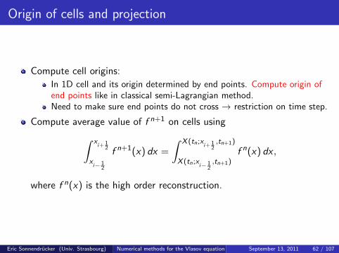
Origin of cells and projection

Compute cell origins:

In 1D cell and its origin determined by end points. Compute origin ofend points like in classical semi-Lagrangian method.Need to make sure end points do not cross → restriction on time step.

Compute average value of f n+1 on cells using∫ xi+ 1

2

xi− 1

2

f n+1(x) dx =

∫ X (tn;xi+ 1

2,tn+1)

X (tn;xi− 1

2,tn+1)

f n(x) dx ,

where f n(x) is the high order reconstruction.


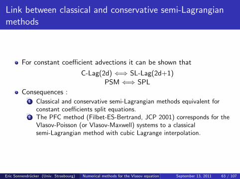
Link between classical and conservative semi-Lagrangianmethods

For constant coefficient advections it can be shown that

C-Lag(2d) ⇐⇒ SL-Lag(2d+1)PSM ⇐⇒ SPL

Consequences :1 Classical and conservative semi-Lagrangian methods equivalent for

constant coefficients split equations.2 The PFC method (Filbet-ES-Bertrand, JCP 2001) corresponds for the

Vlasov-Poisson (or Vlasov-Maxwell) systems to a classicalsemi-Lagrangian method with cubic Lagrange interpolation.


Positive reconstruction

Physical distribution function is always positive.

High-order interpolation can lead to negative values in some zones.

Reconstructed polynomial can be locally modified to remain positive.

Performed for Lagrange reconstruction in PFC method.

Introduces a little more dissipativity, but far less as monotonicreconstructions performed in fluid dynamics.


Simulations

Evolution of L2 norm for N = 128 for SLD

-0.12

-0.1

-0.08

-0.06

-0.04

-0.02

0

0 10 20 30 40 50 60 70 80 90 100

PSM2SPLPSM

PFC2Lag3PFC


Simulations

Evolution of L1 norm for N = 128 for SLD

-0.005

0

0.005

0.01

0.015

0.02

0.025

0.03

0.035

0.04

0.045

0 10 20 30 40 50 60 70 80 90 100

PSM2SPLPSM

PFC2Lag3PFC


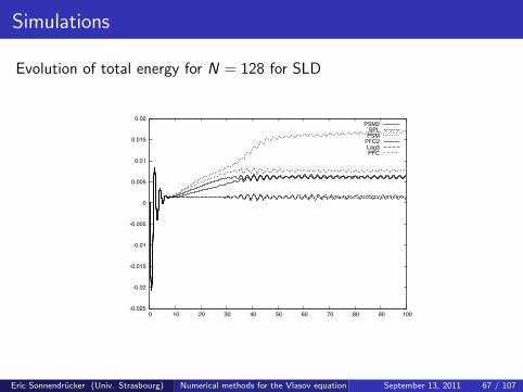
Simulations

Evolution of total energy for N = 128 for SLD

-0.025

-0.02

-0.015

-0.01

-0.005

0

0.005

0.01

0.015

0.02

0 10 20 30 40 50 60 70 80 90 100

PSM2SPLPSM

PFC2Lag3PFC


Simulations

Evolution of total energy for N = 512 for SLD

-0.025

-0.02

-0.015

-0.01

-0.005

0

0.005

0.01

0 10 20 30 40 50 60 70 80 90 100

PSM2SPLPSM

PFC2Lag3PFC


The forward semi-Lagrangian method

f conserved along characteristics

Characteristics advanced with same timeschemes as in PIC method.

Leap-Frog Vlasov-Poisson

Runge-Kutta for guiding-center or gyrokinetic

Values of f deposited on grid of phase space using convolution kernel.

Identical to PIC deposition scheme but in whole phase space insteadof configuration space only.

Similar to PIC method with reconstruction introduced by Denavit(JCP 1972).


Discrete distribution function

Function projected on partition of unity basis for conservativity.Linear B-splines very diffusive. Not useful in practice.Good choice is cubic B-splines.f is reprojected on mesh at each time step.Between tn and tn+1

fh(x , v , t) =∑i ,j

wi ,jB(x − X (t; xi , vj , tn))B(v − X (t; xi , vj , tn)).

The weight wi ,j associated to the particle starting from grid point(xi , vj) at tn is coefficient coefficient of spline satisfying interpolationconditions

fh(xk , vl , tn) =∑i ,j

wi ,jB(xk − xi )B(vk − vj).

Projection on phase space mesh is obtained with formula

f n+1(xk , vl) =∑i ,j

wi ,jB(xk−X (tn+1, xi , vj , tn))B(vl−V (tn+1, xi , vj , tn)).


Time advance for Vlasov-Poisson

As opposite to BSL, trajectories are advanced forward in time.

Advection field is known at initial time. Standard EDO algorithmscan be applied.

For Vlasov-Poisson, we have z(tn) = (xn, vn), andE (tn, zn) = E (tn, xn). Separable Hamiltonian.

Natural scheme is Verlet algorithm, which is second order accurate intime

Step1 : vn+ 12 − vn =

∆t

2E (tn, xn),

Step2 : xn+1 − xn = ∆t vn+1/2,

Step3 : vn+1 − vn+ 12 =

∆t

2E (tn+1, xn+1).


Time advance for guiding-center

Explicit Euler and Runge Kutta have been implemented.Second-order Runge Kutta method

Step1 : X n+1 − X n = ∆tE⊥(tn,X n)

Step2 : Compute E⊥(tn+1,X n+1)

Step3 : X n+1 − X n =∆t

2

[E⊥(tn,X n) + E⊥(tn+1,X n+1)

]Fourth order Runge-Kutta

Step1 : k1 = E⊥(tn,X n)

Step2 : Compute k2 = E⊥(tn+ 12 ,X n +

∆t

2k1)

Step3 : Compute k3 = E⊥(tn+ 12 ,X n +

∆t

2k2)

Step4 : Compute k4 = E⊥(tn+1,X n + ∆tk3)

Step5 : X n+1 − X n =∆t

6[k1 + 2k2 + 2k3 + k4]


Landau damping

f0(x , v) = (1 + 0.001 cos(kx))1√2π

e−v2

2 , L = 4π.

-24

-22

-20

-18

-16

-14

-12

-10

-8

-6

0 20 40 60 80 100

’Runs/thek.dat’ u 1:2-.1533*x - 7.2


Bump on tail (BSL (top) vs. FSL (bottom))

0

5

10

15

20

25

0 1 2 3 4 5 6 7 8

Elec

tric

ener

gy

time

time=0time=20time=30

0

5

10

15

20

25

0 1 2 3 4 5 6 7 8

Elec

tric

ener

gy

time

time=40time=70

time=400

0

5

10

15

20

25

0 1 2 3 4 5 6 7 8

Elec

tric

ener

gy

time

time=0time=20time=30

0

5

10

15

20

25

0 1 2 3 4 5 6 7 8

Elec

tric

ener

gy

time

time=40time=70

time=400


Bump on tail: potential energy (BSL (top) vs. FSL(bottom))

0 1 2 3 4 5 6 7 8 9

0 50 100 150 200 250 300 350 400

Elec

tric

ener

gy

time

0 1 2 3 4 5 6 7 8 9

0 50 100 150 200 250 300 350 400El

ectri

c en

ergy

time


Energy conservation for Kelvin-Helmoltz instability

27.5

28

28.5

29

29.5

30

30.5

31

31.5

0 200 400 600 800 1000

’thdiagO2.dat’ u 1:3’thdiagO4.dat’ u 1:3

’../CG_BSL/thdiag.dat’ u 1:3’thdiag.dat’ u 1:3


FSL vs. BSL

Forward semi-Lagrangian method very promising.

Accurate description of whole phase-space in particular tail ofdistribution function and small perturbations.

A little more diffusive than BSL. Better with smaller time steps.

Some advantages: classical explicit EDO solver can be used, inparticular high order if needed. No need for predictor-corrector orfixed point algorithm.

Can benefit from charge conserving PIC algorithms(Villasenor-Buneman).


A L2-norm conserving Finite Difference scheme

Introduced by Arakawa (1966) for equations of the form

∂f

∂t+ J(ψ, f ) = 0,

for 1D Vlasov ψ = ϕ− v2

2 and J(ψ, f ) = ∂ψ∂x

∂f∂v −

∂ψ∂v

∂f∂x ,

Second and fourth order implemented:

Particle conservation: ddt

∫R2 f (t) dx dv = 0.

Energy conservation: ddt

∫R2 f (t)ψ(t) dx dv = 0.

Conservation of ‖f ‖L2 .


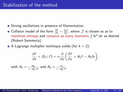
Stabilization of the method

Strong oscillations in presence of filamentation.

Collision model of the form ∂f∂t = ∂J

∂v , where J is chosen so as tomaximize entropy and conserve as many moments

∫fvk dv as desired

(Robert-Sommeria).

A Lagrange multiplier technique yields (for k = 2):

∂f

∂t+ J(ψ, f ) = α

∂

∂v

(∂f

∂v+ A1f − A2fv

),

with A1 = u0

ε−u20/n

, and A2 = nε−u2

0/n.


Evolution of L1 and L2 norms

Figure: Time development of numerical L1 and L2 norms for the non linearLandau damping test.


Evolution of L2 norm and kinetic entropy

Figure: Time development of numerical L2 norm and entropy of f (t) for the twostream instability test.


Computation time

Num. method 32 × 32 pts 32 × 64 pts 32 × 128 pts

FBM 03.33 sec. 05.39 sec. 10.80 sec.

PFC 03.56 sec. 06.28 sec. 11.20 sec.

FDM 17.22 sec. 35.27 sec. 71.20 sec.

SPECTRAL 04.10 sec. 08.25 sec. 16.90 sec.

CIP 13.83 sec. 21.40 sec. 43.24 sec.

SL SPLINE 06.12 sec. 10.55 sec. 20.90 sec.

SL HERMITE 03.60 sec. 06.90 sec. 11.00 sec.


Outline

1 Plasma physics





General ideas

Monitor conservation of invariants:

Number of particles:∫

f (x , v , t) dxdv should be conserved exactlyTotal energyLp norms:

∫|f (x , v , t)|p dxdv in particular L1, L2, L∞.

Analytical solution of equations linearized around an equilibrium.

Analytical solution of linear Vlasov equation: only external field, noself-consistent field.


Outline

1 Plasma physics





Maxwellian equilibrium

1D Vlasov-Poisson. Periodic domain of length L = 2π/k0 in x . WholeR in v . −e charge of electron and m its mass.

Equilibrium distribution solution of Vlasov-Poisson

∂f 0

∂t+ v

∂f 0

∂x− e

mE 0(x)

df 0

dv= 0 (18)

dE 0

dx=

e

ε0(n0 −

∫ +∞

−∞f 0(x , v) dv) (19)

with intial condition f 0(x , v , t) = f0(x , v) and where

n0 = 1L

∫ L0

∫ +∞−∞ f 0(x , v) dx dv is the uniform background neutralizing

density.

Equilibrium f 0(x , v , t) = f0(x , v) = f 0(v). Solution

f 0(v) =n0

2πvthe− v2

2v2th .


Linearization of Vlasov-Poisson around equilibrium

Hilbert expansion around equilibriumf (x , v , t) = f 0(x , v) + εf 1(x , v , t), E (x , t) = E 0(x) + εE 1(x , t) (withE 0(x) = 0).

Plug into Vlasov-Poisson, use fact that f 0 is solution and neglectO(ε2) terms.

Linearized Vlasov-Poisson equation around Maxwellian equilibriumreads

∂f 1

∂t+ v

∂f 1

∂x− e

mE 1(x)

df 0

dv= 0, (20)

dE 1

dx= − e

ε0

∫ +∞

−∞f 1(x , v , t) dv , (21)

with initial condition f 1(x , v , 0) = f 10 (x , v).


Fourier series in x

Consider x 7→ g(x) continuous and L−periodic. It can be expandedinto a Fourier series defined by

g(x) =+∞∑

k ′=−∞g(k)e ikx , g(k) =

1

L

∫ L

0g(x)e−ikx dx , k =

2π

Lk ′.

Apply to f 1. Multiply linearized Vlasov and Poisson by e−ikx andintegrate on one period:

∂ f

∂t(k , v , t) + ikv f (k , v , t)− e

mE (k, t)

df 0

dv= 0, (22)

ikE (k, t) = − e

ε0

∫ +∞

−∞f (k , v , t) dv . (23)

Initial condition satisfies f (k , v , 0) = f0(k, v).


Laplace transform in time

Let ω ∈ C and define Laplace transform by

f (ω) =

∫ +∞

0f (t)e iωt dt for =(ω) > R, (24)

Inverse Laplace transform defined by

f (t) =

∫ +∞+iu

−∞+iuf (ω)e−iωt dω ∀u > R, (25)

such that u analytical in the half space =(ω) > R


Application to linearized Vlasov-Poisson

Multiplying ∂ f∂t (k , v , t) by e iωt and integrating with respect to t

between 0 and +∞, we have∫ +∞

0

∂ f

∂t(k , v , t)e iωt dt = [f (k , v , t)e iωt ]+∞0 − iω

∫ +∞

0f (k , v , t)e iωt dt

= −f (k, v , 0)− iωf (k, v , ω),

where we denote by f (k , v , ω) the Laplace transform of f (k , v , t).

Whence, Laplace transform of Vlasov and Poisson

(−iω + ikv)f (k, v , ω)− e

mE (k, ω)

df 0

dv= f0(k , v), (26)

E (k, ω) =ie

kε0

∫ +∞

−∞f (k, v , ω) dv . (27)


Expression of E (k , ω)

Plug the value of f from Vlasov into Poisson

E =ie

kε0

∫ +∞

−∞

f0(k , v) + em E df 0

dv

−iω + ikvdv =

ie2

kε0mE

∫ +∞

−∞

df 0

dv

−iω + ikvdv +

ie

kε0

∫ +∞

−∞

f0(k , v)

−iω + ikvdv .

Let

D(k , ω) = 1− e2

k2ε0m

∫ +∞

−∞

df 0

dv

v − ωk

dv , N(k , ω) =e

k2ε0

∫ +∞

−∞

f0(k , v)

v − ωk

dv .

Then

E (k , ω) =N(k , ω)

D(k , ω), f (k , v , ω) = i

em E (k , ω)df

0

dv + f0(k , v)

(ω − kv).


Computation of velocity integrals

In the velocity integrals in D and N with have terms of the form

G (ω) =

∫ +∞

−∞

g(v)

v − ωk

dv .

G (ω) is analytical (assuming g is) for =(ω) > 0.

Inverse Laplace transform well defined in this case.

Pole for =(ω) = 0. We need to extend the function to negative valuesof =(ω) by analytical continuation.

Integral in complex plane does not depend on contour as long as thereis no pole between chose contours → instead of choosing real line ascontour for =(ω) > 0 any line unerneath the real line can be chosen.

For analytical continuation for =(ω) ≤ 0 just take integration lineparallel to real line strictly below ω or any deformation of this contourstaying underneath pole.


Examples of contours

Contour for pole on real line (left), underneath real line (right)


The plasma dispersion function

As plasma equilibria are strongly linked to Maxwellians, there is a functionthat naturally appears in calculation of dispersion equations for kineticequations.Fried and Conte called it the plasma dispersion function:

Z (ζ) =1√π

∫γ

e−z2

z − ζdz , (28)

where γ is any contour passing below the pole ζ.


Properties of Z function

Z verifies the following properties

Z (ζ) =1√π

[Pr

∫ +∞

−∞

e−(u+ζ)2

udu + iπe−ζ

2

], (29)

=√πe−ζ

2[i − erfi(ζ)], (30)

where erfi(ζ) = 2√π

∫ ζ0 et

2dt is the complex error function. For b ∈ R

Pr

∫ +∞

−∞

g(u)

u − bdu = lim

δ→0

[∫ b−δ

−∞

g(u)

u − bdu +

∫ +∞

b+δ

g(u)

u − bdu

]is the Cauchy principal value.The derivatives of Z verify:

Z ′(ζ) = −2(1 + ζZ (ζ)),

Z ′′(ζ) = 4ζ − 2(1− 2ζ2)Z (ζ).


Expression of E (x , t)

We got an exact expression for N and D and therefore of E (and f ).

The electric field can be computed by inverse Laplace and Fouriertransform of this expression.

Inverse Laplace transform

E (k , t) =1

2iπ

∫ +∞+iu

−∞+iuE (k , ω)e−iωt dω.

Can be computed using the residue theorem assuming that E (k , ω) isanalytical apart from a finite number of poles. Then

E (k , t) =∑j

Resω=ωj (E (k , ω))e−iωj t ,

the sum being made over the poles which can be computednumerically.


Computation of the residue

E (k , t) =∑j

Resω=ωj E (k , ω)e−iωt , with E (k , ω) =N(k , ω)

D(k, ω)

and the ωj are the roots of D(k , ω) = 0 for fixed k. There are in generalseveral roots of D(k , ω) for a given k . Only the one with largest imaginarypart matters after some time.The residue can be computed thanks to the Taylor expansion of D(k , ω) ina neighborhood of ωj

D(k , ω) = D(k , ωj) + (ω − ωj)∂D

∂ω(k , ωj) + O((ω − ωj)

2),

and so, if ωj is a simple root, we have D(k, ωj) = 0 and ∂D∂ω (k , ωj) 6= 0. So

that

Resω=ωj

(N(k , ω)

D(k, ω)e−iωt

)= lim

ω→ωj

((ω−ωj)N(k , ω)

D(k , ω)e−iωt) =

N(k , ωj)∂D∂ω (k , ω)

e−iωj t .


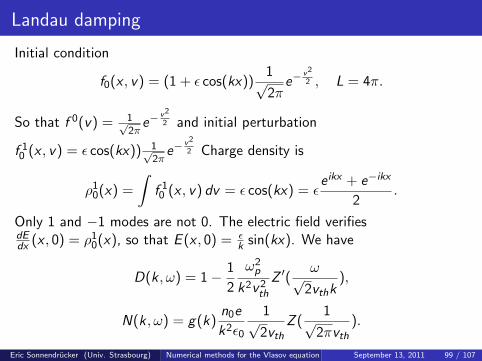
Landau damping

Initial condition

f0(x , v) = (1 + ε cos(kx))1√2π

e−v2

2 , L = 4π.

So that f 0(v) = 1√2π

e−v2

2 and initial perturbation

f 10 (x , v) = ε cos(kx)) 1√

2πe−

v2

2 Charge density is

ρ10(x) =

∫f 10 (x , v) dv = ε cos(kx) = ε

e ikx + e−ikx

2.

Only 1 and −1 modes are not 0. The electric field verifiesdEdx (x , 0) = ρ1

0(x), so that E (x , 0) = εk sin(kx). We have

D(k , ω) = 1− 1

2

ω2p

k2v 2th

Z ′(ω√

2vthk),

N(k , ω) = g(k)n0e

k2ε0

1√2vth

Z (1√

2πvth).


So that

N(k , ω)∂D∂ω (k , ω)

= −2g(k)m

ekv 2

th

Z ( ω√2vthk

)

Z ′′( ω√2vthk

)(31)

= −g(k)m

ekv 2

th

Z ( ω√2vthk

)

2 ω√2vthk

− (1− ω2

v2thk

2 )Z ( ω√2vthk

). (32)

Dominant roots of dispersion relation

k ωjN(k,ωj )∂D∂ω

(k,ωj )

0.5 ±1.4156− 0.1533i 0.3677 e±i0.536245

0.4 ±1.2850− 0.0661i 0.424666 e±i0.3357725

0.3 ±1.1598− 0.0126i 0.63678 e±i0.114267

0.2 ±1.0640− 5.510× 10−5i 1.129664 e±i0.00127377

Denote by ωr = <(ωj), ωi = =(ωj), r the amplitude ofN(k,ωj )∂D∂ω

(k,ωj )and ϕ its

phase.


Linear solution of Landau damping

Maple code for dispersion relation

k := 0.2;

dd := w− > 1 + (1/k ∗ ∗2) ∗ (1 + sqrt(Pi/2) ∗ w/k

∗ exp(−w ∗ ∗2/(2 ∗ k ∗ ∗2)) ∗ (−erfi(w/(sqrt(2) ∗ k)) + I ));

root2 := fsolve(dd(w),w = 1, complex);

Dominant solution for E

E (k , t) ≈ re iϕe−i(ωr+iωi )t + re−iϕe−i(−ωr+iωi )t ,

= reωi t(e−i(ωr t−ϕ) + e i(ωr t−ϕ)),

= 2reωi t cos(ωr t − ϕ).

Then as E (−k, t) = −E (k, t), we have

E (x , t) ≈ 4εreωi t sin(kx) cos(ωr t − ϕ).


Analytical solution and computed solution for k=0.4

f0(x , v) = (1 + 0.001 cos(kx))1√2π

e−v2

2 , L = 4π.

Dominant analytical solution

E (k , t) = 0.002× 0.424666e0.0661t cos(1.2850t − 0.3357725)

-20

-18

-16

-14

-12

-10

-8

-6

0 5 10 15 20 25 30 35 40 45 50

’Runs/thek.dat’log(0.002*0.42466*abs(cos(1.285*x-0.33577))*exp(-0.0661*x))


Two stream instability (1/2)

Dispersion relation

D(k , ω) = 1 +ω2p

2k2v 2th

[2+√π

2

(ω

vthk− v0

vth

)e−

( ωk−v0)2

2v2th (i − erfi(

ωk − v0√

2vth)

√π

2

(ω

vthk+

v0

vth

)e−

( ωk

+v0)2

2v2th (i − erfi(

ωk + v0√

2vth)

,

Some roots for k = 0.2

v0 ω ω

1.3 0.02115i 1.1648− 0.00104i2.4 0.2258i 1.3390− 0.00242i3.0 0.2845i 1.446− 0.00299i


Two stream instability (2/2)

Maple code

k := 0.2; v0 := 3;

dd := w− > 1 + (1/(2 ∗ k ∗ ∗2)) ∗ ((1 + sqrt(Pi/2) ∗ (w/k − v0)

∗ exp(−(w/k − v0) ∗ ∗2/2) ∗ (−erfi((w/k − v0)/sqrt(2)) + I ))

+ (1 + sqrt(Pi/2) ∗ (w/k + v0) ∗ exp(−(w/k + v0) ∗ ∗2/2)

∗ (−erfi((w/k + v0)/sqrt(2)) + I )));



Initial condition

f0(x , v) = (1 + 0.001 cos(kx))1

2√

2π(e−

(v−v0)2

2 + e−(v+v0)2

2 ), L =2π

k.


k=0.2; v0=1.3

-12

-11

-10

-9

-8

-7

-6

-5

0 10 20 30 40 50

’Runs/thek.dat’ u 1:2-0.001*x -6.2


k=0.2; v0=2.4

-12

-10

-8

-6

-4

-2

0

2

4

0 10 20 30 40 50

’Runs/thek.dat’ u 1:20.2258*x -8.4


k=0.2; v0=3

-10

-8

-6

-4

-2

0

2

4

6

8

0 10 20 30 40 50

’Runs/thek.dat’ u 1:2.2845*x -8.2


numerical methods for the vlasov equation

Documents