numerical methods for sparse recovery -...
TRANSCRIPT
Radon Series Comp. Appl. Mathxx, 1–110 c© de Gruyter 2010
Numerical Methods for Sparse Recovery
Massimo Fornasier
Abstract. These lecture notes address the analysis of numerical methods for performing opti-mizations with linear model constraints and additional sparsity conditions to solutions, i.e., weexpect solutions which can be represented as sparse vectorswith respect to a prescribed basis.In the first part of the manuscript we illustrate the theory ofcompressed sensing with emphasison computational aspects. We present the analysis of the homotopy method, the iterativelyre-weighted least squares method, and the iterative hard-thresholding. In the second part, start-ing from the analysis of iterative soft-thresholding, we illustrate several numerical methods foraddressing sparse optimizations in Hilbert spaces. The third and final part is concerned withnumerical techniques, based on domain decomposition methods, for dimensionality reductionin large scale computing. In the notes we are mainly focusingon the analysis of the algorithms,and we report a few illustrative numerical examples.
Key words. Numerical methods for sparse optimization, calculus of variations, algorithms fornonsmooth optimization.
AMS classification.15A29, 65K10, 90C25, 52A41, 49M30.
1 Introduction
These lecture notes are an introduction to methods recentlydeveloped for performingnumerical optimizations with linear model constraints andadditional sparsity condi-tions to solutions, i.e., we expect solutions which can be represented as sparse vectorswith respect to a prescribed basis. Such a type of problems has been recently greatlypopularized by the development of the field of nonadaptive compressed acquisition ofdata, the so-calledcompressed sensing, and its relationship withℓ1-minimization. Westart our presentation by recalling the mathematical setting of compressed sensing as areference framework for developing further generalizations. In particular we focus onthe analysis of algorithms for such problems and their performances. We introduce andanalyse the homotopy method, the iteratively reweighted least squares method, and theiterative hard thresholding algorithm. We will see that theproperties of convergenceof these algorithms to solutions depend very much on specialspectral properties, theRestricted Isometry Property or the Null Space Property, ofthe matrices which definethe linear models. This provides a link to the analysis of random matrices which aretypical examples of matrices with such properties. The concept of sparsity does notnecessarily affect the entries of a vector only, but it can also be applied, for instance,to their variation. We will show that some of the algorithms proposed for compressedsensing are in fact useful for optimization problems with total variation constraints.
2 M. Fornasier
These optimizations on continuous domains are related to the calculus of variations onbounded variation (BV) functions and to geometric measure theory.In the second part of the lecture notes we address sparse optimizations in Hilbertspaces, and especially for situations where no Restricted Isometry Property or NullSpace Property are assumed for the linear model. We will be able to formulate effi-cient algorithms based on so-callediterative soft-thresholdingalso for such situations,although their analysis will require different tools, typically from nonsmooth convexanalysis.A common feature of the illustrated algorithms will be theirvariational nature, in thesense that they are derived as minimization strategies of given energy functionals. Notonly does the variational framework allow us to derive very precise statements aboutthe convergence properties of these algorithms, but it alsoprovides the algorithms withan intrinsic robustness.We will finally address large scale computations, showing how we can define domaindecomposition strategies for these nonsmooth optimizations, for problems comingfrom compressed sensing andℓ1-minimization as well as for total variation minimiza-tion problems.The first part of the lecture notes is elementary and it does not require more than thebasic knowledge of notions of linear algebra and standard inequalities. The secondpart of the course is slightly more advanced and addresses problems in Hilbert spaces,and we will make use of concepts of nonsmooth convex analysis. We refer the inter-ested reader to the books [36, 50] for an introduction to convex analysis, variationalmethods, and related numerical techniques.
Acknowledgement
I’m very grateful to the colleagues Antonin Chambolle, Ronny Ramlau, Holger Rauhut,Jared Tanner, Gerd Teschke, and Mariya Zhariy for acceptingthe invitation to pre-pare and present a course at the Johann Radon Institute for Computational and Ap-plied Mathematics (RICAM) of the Austrian Academy of Sciences during the Sum-mer School “Theoretical Foundations and Numerical Methodsfor Sparse Recovery”.Also these lecture notes were prepared on this occasion. Furthermore I would liketo thank especially Wolfgang Forsthuber, Madgalena Fuchs,Andreas Langer, and An-nette Weihs for the enormous help they provided us for the organization of the SummerSchool. I acknowledge the financial support of RICAM, of the Doctoral Program inComputational Mathematics of the Johannes Kepler University of Linz, and the sup-port by the project Y 432-N15 START-Preis “Sparse Approximation and Optimizationin High Dimensions”.
Numerical Methods for Sparse Recovery 3
1.1 Notations
In the following we collect general notations. More specificnotations will be intro-duced and recalled in the following sections.We will considerX = R
N as a Banach space endowed with different norms. Inparticular, later we use theℓp-(quasi-)norms
‖x‖p := ‖x‖ℓp := ‖x‖ℓNp
:=
(∑Ni=1 |xj |p
)1/p, 0< p <∞,
maxj=1,...,N |xj |, p = ∞.(1.1)
Associated to these norms we denote their unit balls byBℓp := BℓNp
:= x ∈ R :
‖x‖p ≤ 1 and the balls of radiusR by Bℓp(R) := BℓNp
(R) := R · BℓNp
. As-
sociated to a closed convex body 0∈ Ω ⊂ RN , we define its polar set byΩ =
y ∈ RN : supx∈Ω〈x, y〉 ≤ 1. This allow us to define an associated norm‖x‖Ω =
supy∈Ω〈x, y〉.The index setI is supposed to be countable and we will consider theℓp(I) spaces ofp-summable sequences over the index setI as well. Their norm are defined as usualand similarly to the case ofRN . We use the same notationsBℓp for theℓp(I)-balls asfor the ones inRN . With A we will usually denote am × N real matrix,m,N ∈ N
or an operatorA : ℓ2(I) → Y . We denote withA∗ the adjoint matrix or withK∗ theadjoint of an operatorK. We will always work on real vector spaces, hence, in finitedimensions,A∗ usually coincides with the transposed matrix ofA. The norm of anoperatorK : X → Y acting between two Banach spaces is denoted by‖K‖X→Y ; formatrices the norm‖A‖ denotes the spectral norm. The support of a vectoru ∈ ℓ2(I),i.e., the set of coordinates which are not zero, is denoted bysupp(u).We will consider index setsΛ ⊂ I and their complementsΛc = I \ Λ. The symbols|Λ| and#Λ are used indifferently for indicating the cardinality ofΛ. With a slightabuse we will denote
‖u‖0 := ‖u‖ℓ0(I) := # supp(u), (1.2)
which is popularly called the “ℓ0-norm” in the literature. When#I = N thenℓ2(I) =R
N and we may also denote‖u‖ℓN0
:= ‖u‖ℓ0(I) We use the notationAΛ to indicatea submatrix extracted fromA by retaining only the columns indexed inΛ as well asthe restrictionsuΛ of vectorsu to the index setΛ. We also denote byA∗AΛ×Λ :=(A∗A)Λ×Λ := A∗
ΛAΛ the submatrix extracted fromA∗A by retaining only the entriesindexed onΛ × Λ.Generic positive constants used in estimates are denoted asusual by
c, C, c, C, c0, C0, c1, C1, c2, C2, . . . .
4 M. Fornasier
2 An Introduction to Sparse Recovery
2.1 A Toy Mathematical Model for Sparse Recovery
2.1.1 Adaptive and Compressed Acquisition
Let k,N ∈ N, k ≤ N and
Σk := x ∈ RN : ‖x‖ℓN
0:= # supp(x) ≤ k,
be the set of vectors with at mostk nonzero entries, which we will callk-sparse vec-tors. Thek-best approximation errorthat we can achieve in this set to a vectorx ∈ R
N
with respect to a suitable space quasi-norm‖ · ‖X is defined by
σk(x)X = infz∈Σk
‖x− z‖X .
Example 2.1 Let r(x) be thenonincreasing rearrangementof x, i.e.,
r(x) = (|xi1|, . . . , |xiN |)T and|xij | ≥ |xij+1|, for j = 1, . . . ,N − 1.
Then it is straightforward to check that
σk(x)ℓNp
:=
N∑
j=k+1
rj(x)p
1/p
, 1 ≤ p <∞.
In particular, the vectorx[k] derived fromx by setting to zero all theN − k smallestentries in absolute value is called thebestk-term approximationto x and it coincideswith
x[k] = arg minz∈Σk
‖x− z‖ℓNp. (2.3)
for any 1≤ p <∞.
Lemma 2.2 Let r = 1q − 1
p andx ∈ RN . Then
σk(x)ℓp ≤ ‖x‖ℓqk−r, k = 1,2, . . . ,N.
Proof. Let Λ be the set of indexes of ak-largest entries ofx in absolute value. Ifε = rk(x), thekth-entry of the nonincreasing rearrangementr(x), then
ε ≤ ‖x‖ℓqk− 1
q .
Therefore
σk(x)pℓp
=∑
j /∈Λ
|xj|p ≤∑
j /∈Λ
εp−q|xj |q
≤ ‖x‖p−qℓq
k− p−q
q ‖x‖qℓq,
Numerical Methods for Sparse Recovery 5
which impliesσk(x)ℓp ≤ ‖x‖ℓqk
−r.
The computation of the bestk-term approximation ofx ∈ RN in general requires the
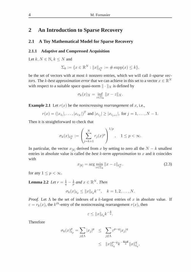
search of the largest entries ofx in absolute value, and therefore the testing of all theentries of the vectorx. This procedure isadaptive, since it depends on the particularvector, and it is currently at the basis of lossy compressionmethods, such as JPEG [58].
2.1.2 Nonadaptive and Compressed Acquisition: CompressedSensing
One would like to describe alinear encoderwhich allows us to compute approximatelyk measurements(y1, . . . , yk)
T and a nearly optimal approximation ofx in the follow-ing sense:
Provided a setK ⊂ RN , there exists a linear mapA : R
N → Rm,
with m ≈ k and a possibly nonlinear map∆ : Rm → R
N such that
‖x− ∆(Ax)‖X ≤ Cσk(x)X
for all x ∈ K.
Note that the way we encodey = Ax is via a prescribed mapA which is indepen-dent ofx. Also the decoding procedure∆ might depend onA, but not onx. Thisis why we call this strategy anonadaptive (or universal) and compressed acquisitionof x. Note further that we would like to recover an approximationto x from nearlyk-linear measurements which is of the order of thek-best approximation error. In thissense we say that the performances of the encoder/decoder system(A,∆) is nearlyoptimal.
2.1.3 Optimal Performances of Encoder/Decoder Pairs
Let us defineAm,N the set of all encoder/decoder pairs(A,∆) with A a m × Nmatrix and∆ : R
m → RN any function. We wonder whether there exists such a
nearly optimal pair as claimed above. Let us fixm ≤ N two natural numbers, andK ⊂ R
N . For 1≤ k ≤ N we denote
σk(K)X := supx∈K
σk(x)X , andEm(K)X := inf(A,∆)∈Am,N
supx∈K
‖x− ∆(Ax)‖X .
We would like to find the largestk such that
Em(K)X ≤ C0σk(K)X .
We answer this question in the particular case whereK = BℓN1
andX = ℓN2 . Thissetting will turn out to be particularly useful later on and it is already sufficient for
6 M. Fornasier
showing that, unfortunately, it is impossible to reconstruct x ∈ BℓN1
with an accuracyasymptotically (form,N larger and larger) of the order of thek-best approximationerror inℓM2 if k = m, but it is necessary to have a slightly larger number of measure-ments, i.e.,k = m− ε(m,N), ε(m,N) > 0.
The proper estimate ofEm(K)X turns out to be linked to the geometrical conceptof Gelfand width.
Definition 2.3 Let K be a compact set inX. Then theGelfand widthof K of orderm is
dm(K)X := infY ≤ X
codim(Y ) ≤ m
sup‖x‖X : x ∈ K ∩ Y .
The infimum is taken over the set of linear subspacesY of X with codimension lessof equal tom.
We have the following fundamental equivalence.
Proposition 2.4 LetK ⊂ RN be any closed compact set for whichK = −K and
such that there exists a constantC0 > 0 for whichK +K ⊂ C0K. If X ⊂ RN is a
normed space, then
dm(K)X ≤ Em(K)X ≤ C0dm(K)X .
Proof. For a matrixA ∈ Rm×N , we denoteN = kerA. Note thatY = N has codi-
mension less or equal thanm. Conversely, given any spaceY ⊂ RN of codimension
less or equal thanm, we can associate a matrixA whose rows are a basis forY ⊥. Withthis identification we see that
dm(K)X = infA∈Rm×N
sup‖η‖X : η ∈ N ∩K.
If (A,∆) is an encoder/decoder pair inAm,N andz = ∆(0), then for anyη ∈ N wehave also−η ∈ N . It follows that either‖η − z‖X ≥ ‖η‖X or ‖ − η − z‖X ≥ ‖η‖X .Indeed, if we assumed that both were false then
‖2η‖X = ‖η − z + z + η‖X ≤ ‖η − z‖X + ‖ − η − z‖X < 2‖η‖X ,
a contradiction. SinceK = −K we conclude that
dm(K)X = infA∈Rm×N
sup‖η‖X : η ∈ N ∩K
≤ supη∈N∩K
‖η − z‖X
= supη∈N∩K
‖η − ∆(Aη)‖X
≤ supx∈K
‖x− ∆(Ax)‖X .
Numerical Methods for Sparse Recovery 7
By taking the infimum over all(A,∆) ∈ Am,N we obtain
dm(K)X ≤ Em(K)X .
To prove the upper inequality, let us choose an optimalY such that
dm(K)X = sup‖x‖X : x ∈ Y ∩K.
(Actually such an optimal subspaceY always exists [54].) As mentioned above, wecan associate toY a matrixA such thatN = kerA = Y . Let us denote the affinesolution spaceF(y) := x : Ax = y. Let us now define a decoder as follows: IfF(y) ∩K 6= ∅ then we takex(y) ∈ F(y) ∩K and∆(y) = x(y). If F(y) ∩K = ∅then∆(y) ∈ F(y). Hence, we can estimate
Em(K)X = inf(A,∆)∈Am,N
supx∈K
‖x− ∆(Ax)‖X
≤ supx,x′∈K;Ax=Ax′
‖x− x′‖X
≤ supη∈C0(N∩K)
‖η‖X ≤ C0dm(K)X .
The following result was proven in the relevant work of Kashin, Garnaev, andGluskin [46, 47, 51] already in the ’70s and ’80s. See [20, 33]for a description ofthe relationship between this result and the more modern point of view on compressedsensing.
Theorem 2.5 The Gelfand widths ofℓNq -balls in ℓNp for 1 ≤ q < p ≤ 2 are estimatedby
C1Ψ(m,N, p, q) ≤ dm(BℓNq
)ℓNp≤ C2Ψ(m,N, p, q),
where
Ψ(m,N, p, q) = min
1, N1− 1qm− 1
2
1/q−1/p1/q−1/2
, 1< q < p ≤ 2
Ψ(m,N,2,1) = min
1,√
log(N/m)+1m
, q = 1 andp = 2.
From Proposition 2.4 and Theorem 2.5 we obtain
C1Ψ(m,N, p, q) ≤ Em(BℓNq
)ℓNp≤ C2Ψ(m,N, p, q).
In particular, forq = 1 andp = 2, we obtain, form,N large enough, the estimate
C1
√log(N/m) + 1
m≤ Em(BℓN
1)ℓN
2.
8 M. Fornasier
If we wanted to enforce
Em(BℓN1
)ℓN2≤ Cσk(BℓN
1)ℓN
2,
then Lemma 2.2 would imply√
log(N/m) + 1m
≤ C0k− 1
2 , or k ≤ C0m
log Nm + 1
.
Hence, we proved the following
Corollary 2.6 Form,N fixed, there exists an optimal encoder/decoder pair(A,∆) ∈Am,N , in the sense that
Em(BℓN1
)ℓN2≤ Cσk(BℓN
1)ℓN
2,
only if
k ≤ C0m
log Nm + 1
, (2.4)
for some constantC0 > 0 independent ofm,N .
The next section is devoted to the construction of optimal encoder/decoder pairs(A,∆) ∈Am,N as stated in the latter corollary.
2.2 Survey on Mathematical Analysis of Compressed Sensing
In the following sections we want to show that under a certainproperty, called theRestricted Isometry Property(RIP) for a matrixA,
The decoder, which we callℓ1-minimization,
∆(y) = arg minAz=y=Ax
‖z‖ℓN1
(2.5)
performs‖x− ∆(y)‖ℓN
1≤ C1σk(x)ℓN
1, (2.6)
as well as
‖x− ∆(y)‖ℓN2≤ C2
σk(x)ℓN1
k1/2, (2.7)
for all x ∈ RN .
Note that by (2.7) we immediately obtain
Em(BℓN1
)ℓN2≤ C0k
−1/2,
implying once again (2.4). Hence, the following question wewill address is the exis-tence of matricesA with RIP for whichk is optimal, i.e.,
k ≍ m
logN/m + 1.
Numerical Methods for Sparse Recovery 9
2.2.1 An Intuition Why ℓ1-Minimization Works Well
In this section we would like to provide an intuitive explanation of the near-optimalerror estimates (2.6) and (2.7) provided byℓ1-minimization (2.5) in recovering vectorsfrom partial linear measurements. Equations (2.6) and (2.7) ensure in particular that ifthe vectorx is k-sparse, thenℓ1-minimization (2.5) will be able to recover itexactlyfromm linear measurementsy obtained via the matrixA. This result is quite surprisingbecause the problem of recovering a sparse vector, or the solution of the followingoptimization
min ‖x‖ℓN0
subject toAx = y, (2.8)
is know to beNP-complete1 [59, 61] whereasℓ1-minimization is a convex problemwhich can be solved at any prescribed accuracy in polynomialtime. For instanceinterior-point methods are guaranteed to solve theℓ1-problem to a fixed precision intimeO(m2N1.5) [63]. The first intuitive approach to this perhaps surprising result isby interpretingℓ1-minimization as theconvex relaxationof the problem (2.8).
-4 -2 0 2 40
5
10
15
20
25
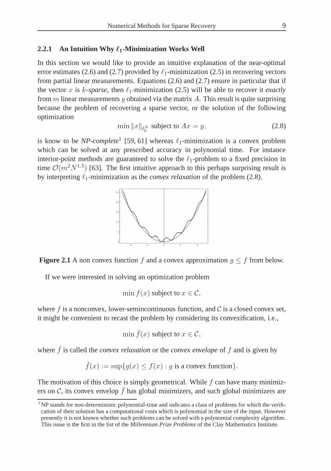
Figure 2.1A non convex functionf and a convex approximationg ≤ f from below.
If we were interested in solving an optimization problem
min f(x) subject tox ∈ C,
wheref is a nonconvex, lower-semincontinuous function, andC is a closed convex set,it might be convenient to recast the problem by considering its convexification, i.e.,
min f(x) subject tox ∈ C,
wheref is called theconvex relaxationor theconvex envelopeof f and is given by
f(x) := supg(x) ≤ f(x) : g is a convex function.
The motivation of this choice is simply geometrical. Whilef can have many minimiz-ers onC, its convex envelopf has global minimizers, and such global minimizers are
1 NP stands for non-deterministic polynomial-time and indicates a class of problems for which the verifi-cation of their solution has a computational costs which is polynomial in the size of the input. Howeverpresently it is not known whether such problems can be solvedwith a polynomial complexity algorithm.This issue is the first in the list of theMillennium Prize Problemsof the Clay Mathematics Institute.
10 M. Fornasier
likely to be in a neighborhood of a global minimizer off , see Figure 2.1. Actually ifC is compact, then the global minima off andf must necessarily coincide. Unfortu-nately, the precise computation off is again a very difficult problem. In the case of
0.2 0.4 0.6 0.8 1
0.2
0.4
0.6
0.8
1
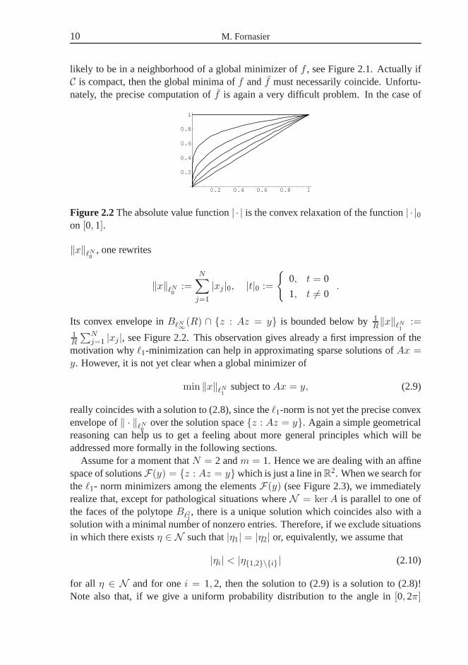
Figure 2.2The absolute value function| · | is the convex relaxation of the function| · |0on [0,1].
‖x‖ℓN0
, one rewrites
‖x‖ℓN0
:=
N∑
j=1
|xj |0, |t|0 :=
0, t = 0
1, t 6= 0.
Its convex envelope inBℓN∞
(R) ∩ z : Az = y is bounded below by1R‖x‖ℓN
1:=
1R
∑Nj=1 |xj|, see Figure 2.2. This observation gives already a first impression of the
motivation whyℓ1-minimization can help in approximating sparse solutions of Ax =y. However, it is not yet clear when a global minimizer of
min ‖x‖ℓN1
subject toAx = y, (2.9)
really coincides with a solution to (2.8), since theℓ1-norm is not yet the precise convexenvelope of‖ · ‖ℓN
0over the solution spacez : Az = y. Again a simple geometrical
reasoning can help us to get a feeling about more general principles which will beaddressed more formally in the following sections.
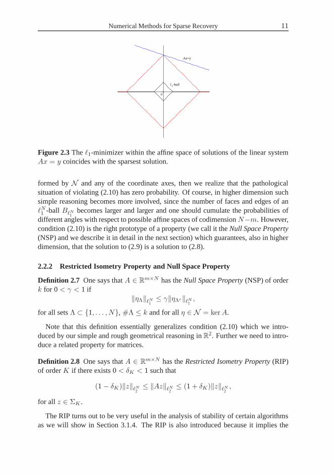
Assume for a moment thatN = 2 andm = 1. Hence we are dealing with an affinespace of solutionsF(y) = z : Az = ywhich is just a line inR2. When we search forthe ℓ1- norm minimizers among the elementsF(y) (see Figure 2.3), we immediatelyrealize that, except for pathological situations whereN = kerA is parallel to one ofthe faces of the polytopeBℓ2
1, there is a unique solution which coincides also with a
solution with a minimal number of nonzero entries. Therefore, if we exclude situationsin which there existsη ∈ N such that|η1| = |η2| or, equivalently, we assume that
|ηi| < |η1,2\i| (2.10)
for all η ∈ N and for onei = 1,2, then the solution to (2.9) is a solution to (2.8)!Note also that, if we give a uniform probability distribution to the angle in[0,2π]
Numerical Methods for Sparse Recovery 11
0
Az=y
l1-ball
Figure 2.3 Theℓ1-minimizer within the affine space of solutions of the linearsystemAx = y coincides with the sparsest solution.
formed byN and any of the coordinate axes, then we realize that the pathologicalsituation of violating (2.10) has zero probability. Of course, in higher dimension suchsimple reasoning becomes more involved, since the number offaces and edges of anℓN1 -ball BℓN
1becomes larger and larger and one should cumulate the probabilities of
different angles with respect to possible affine spaces of codimensionN−m. However,condition (2.10) is the right prototype of a property (we call it the Null Space Property(NSP) and we describe it in detail in the next section) which guarantees, also in higherdimension, that the solution to (2.9) is a solution to (2.8).
2.2.2 Restricted Isometry Property and Null Space Property
Definition 2.7 One says thatA ∈ Rm×N has theNull Space Property(NSP) of order
k for 0< γ < 1 if‖ηΛ‖ℓN
1≤ γ‖ηΛc‖ℓN
1,
for all setsΛ ⊂ 1, . . . , N, #Λ ≤ k and for allη ∈ N = kerA.
Note that this definition essentially generalizes condition (2.10) which we intro-duced by our simple and rough geometrical reasoning inR
2. Further we need to intro-duce a related property for matrices.
Definition 2.8 One says thatA ∈ Rm×N has theRestricted Isometry Property(RIP)
of orderK if there exists 0< δK < 1 such that
(1− δK)‖z‖ℓN2≤ ‖Az‖ℓN
2≤ (1 + δK)‖z‖ℓN
2,
for all z ∈ ΣK .
The RIP turns out to be very useful in the analysis of stability of certain algorithmsas we will show in Section 3.1.4. The RIP is also introduced because it implies the
12 M. Fornasier
Null Space Property, and when dealing with random matrices (see Section 2.2.4) it ismore easily addressed. In fact we have:
Lemma 2.9 Assume thatA ∈ Rm×N has the RIP of orderK = k+h with 0< δK <
1. ThenA has the NSP of orderk and constantγ =√
kh
1+δK1−δK
.
Proof. LetΛ ⊂ 1, . . . , N, #Λ ≤ k. DefineΛ0 = Λ andΛ1,Λ2, . . . ,Λs disjoint setsof indexes of size at mosth, associated to a decreasing rearrangement of the entries ofη ∈ N = ker(A). Then, by using Cauchy-Schwarz inequality, the RIP twice, the factthatAη = 0, and eventually the triangle inequality, we have the following sequence ofinequalities:
‖ηΛ‖ℓN1
≤√k‖ηΛ‖ℓN
2≤
√k‖ηΛ0∪Λ1‖ℓN
2
≤ (1− δK)−1√k‖AηΛ0∪Λ1‖ℓN
2= (1− δK)−1
√k‖AηΛ2∪Λ3∪···∪Λs‖ℓN
2
≤ (1− δK)−1√k
s∑
j=2
‖AηΛj‖ℓN2≤ 1 + δK
1− δK
√k
s∑
j=2
‖ηΛj‖ℓN2. (2.11)
Note now thati ∈ Λj+1 andℓ ∈ Λj imply by construction ofΛ′js by nonincreasing
rearrangement of the entries ofη
|ηi| ≤ |ηℓ|.
By taking the sum overℓ first and than theℓN2 -norm overi we get
|ηi| ≤ h−1‖ηΛj‖ℓN1, and‖ηΛj+1‖ℓN
2≤ h−1/2‖ηΛj‖ℓN
1.
By using the latter estimates in (2.11) we obtain
‖ηΛ‖ℓN1≤ 1 + δK
1− δK
√k
h
s−1∑
j=1
‖ηΛj‖ℓN1≤(
1 + δK1− δK
√k
h
)‖ηΛc‖ℓN
1.
The RIP property does imply the NSP, but the converse is not true. Actually the RIPis significantly more restrictive.
2.2.3 Performances ofℓ1-Minimization as an Optimal Decoder
In this section we address the proofs of the approximation properties (2.6) and (2.7).
Theorem 2.10 Let A ∈ Rm×N satisfy the RIP of order2k with δ2k ≤ δ <
√2−1√2+1
(or simplyA satisfies the NSP of orderk with constantγ = 1+δ1−δ
√12 < 1) , then the
decoder∆ as in(2.5)satisfies(2.6).
Numerical Methods for Sparse Recovery 13
Proof. By Lemma 2.9 we have
‖ηΛ‖ℓN1≤ 1 + δ
1− δ
√12‖ηΛc‖ℓN
1,
for all Λ ⊂ 1, . . . , N, #Λ ≤ k andη ∈ N = kerA. Let x∗ = ∆(Ax), so thatη = x∗ − x ∈ N , and
‖x∗‖ℓN1≤ ‖x‖ℓN
1.
One denotes now withΛ the set of thek-largest entries ofx in absolute value. One has
‖x∗Λ‖ℓN1
+ ‖x∗Λc‖ℓN1≤ ‖xΛ‖ℓN
1+ ‖xΛc‖ℓN
1.
It follows immediately by triangle inequality
‖xΛ‖ℓN1− ‖ηΛ‖ℓN
1+ ‖ηΛc‖ℓN
1− ‖xΛc‖ℓN
1≤ ‖xΛ‖ℓN
1+ ‖xΛc‖ℓN
1.
Hence
‖ηΛc‖ℓN1≤ ‖ηΛ‖ℓN
1+ 2‖xΛc‖ℓN
1≤ 1 + δ
1− δ
√12‖ηΛc‖ℓN
1+ 2σk(x)ℓN
1,
or, equivalently,
‖ηΛc‖ℓN1≤ 2
1− 1+δ1−δ
√12
σk(x)ℓN1. (2.12)
In particular, note that forδ <√
2−1√2+1
we have1+δ1−δ
√12 < 1. Eventually we conclude
the estimates
‖x− x∗‖ℓN1
= ‖ηΛ‖ℓN1
+ ‖ηΛc‖ℓN1
≤(
1 + δ
1− δ
√12
+ 1
)‖ηΛc‖ℓN
1
≤ C1σk(x)ℓN1,
whereC1 :=
2
„1+δ1−δ
q12+1
«
1− 1+δ1−δ
q12
.
Similarly we address the second estimate (2.7).
Theorem 2.11 LetA ∈ Rm×N satisfy the RIP of order3k with δ3k ≤ δ <
√2−1√2+1
, thenthe decoder∆ as in(2.5)satisfies(2.7).
14 M. Fornasier
Proof. Letx∗ = ∆(Ax). As we proceeded in Lemma 2.9, we denoteη = x∗−x ∈ N ,Λ0 = Λ the set of the 2k-largest entries ofη in absolute value, andΛj of size at mostk composed of nonincreasing rearrangement entries ofη. Then
‖ηΛ‖ℓN2≤ 1 + δ
1− δk−
12‖ηΛc‖ℓN
1.
Note now that by Lemma 2.2 and by Lemma 2.9
‖ηΛc‖ℓN2
≤ (2k)−12‖η‖ℓN
1= (2k)−1/2
(‖ηΛ‖ℓN
1+ ‖ηΛc‖ℓN
1
)
≤ (2k)−1/2(C‖ηΛc‖ℓN
1+ ‖ηΛc‖ℓN
1
)
=C + 1√
2k−1/2‖ηΛc‖ℓN
1,
for a suitable constantC > 0. Note that, beingΛ the set of the in absolute value2k-largest entries ofη, one has also
‖ηΛc‖ℓN1≤ ‖η(supp x[2k])c‖ℓN
1≤ ‖η(supp x[k])c‖ℓN
1, (2.13)
wherex[h] is the besth-term approximation tox. The use of this latter estimate,combined with inequality (2.12) finally gives
‖x− x∗‖ℓN2
≤ ‖ηΛ‖ℓN2
+ ‖ηΛc‖ℓN2
≤ C1k−1/2‖ηΛc‖ℓN
1
≤ C2k−1/2σk(x)ℓN
1.
We would like to conclude this section by mentioning a further stability property ofℓ1-minimization as established in [12].
Theorem 2.12 LetA ∈ Rm×N which satisfies the RIP of order4k with δ4k sufficiently
small. Assume further thatAx + e = y wheree is a measurement error. Then thedecoder∆ has the further enhanced stability property:
‖x− ∆(y)‖ℓN2≤ C3
(σk(x)ℓN
2+σk(x)ℓN
1
k1/2+ ‖e‖ℓN
2
). (2.14)
2.2.4 Random Matrices and Optimal RIP
In this section we would like to mention how, for different classes of random matrices,it is possible to show that the RIP property can hold with optimal constants, i.e.,
k ≍ m
logN/m + 1.
at least with high probability. This implies in particular,that such matrices exist, theyare frequent, but they are given to us only with an uncertainty.
Numerical Methods for Sparse Recovery 15
Gaussian and Bernoulli random matrices
Let (Ω,P) be a probability space andX a random variable on(Ω,P). One can de-fine a random matrixA(ω), ω ∈ ΩmN , as the matrix whose entries are independentrealizations ofX . We assume further that‖A(ω)x‖2
ℓN2
has expected value‖x‖2ℓN
2and
P
(∣∣∣‖A(ω)x‖2ℓN
2− ‖x‖2
ℓN2
∣∣∣ ≥ ε‖x‖2ℓN
2
)≤ 2e−mc0(ε), 0< ε < 1. (2.15)
Example 2.13 Here we collect two relevant examples for which the concentrationproperty (2.15) holds:
1. One can choose, for instance, the entries ofA as i.i.d. Gaussian random variables,Aij ∼ N (0, 1
m), andc0(ε) = ε2/4 − ε3/6. This can be shown by using Chernoffinequalities and a comparison of the moments of a Bernoulli random variable withrespect to those of a Gaussian random variable;
2. One can also use matrices where the entries are independent realizations of±1Bernoulli random variables, i.e.,
Aij =
+1/
√m, with probability 1
2
−1/√m, with probability 1
2
.
Then we have the following result, shown, for instance in [3].
Theorem 2.14 Suppose thatm,N and0 < δ < 1 are fixed. IfA(ω), ω ∈ ΩmN is arandom matrix of sizem×N with the concentration property(2.15), then there existconstantsc1, c2 > 0 depending onδ such that the RIP holds forA(ω) with constantδandk ≤ c1
mlog(N/m)+1 with probability exceeding1− 2e−c2m.
An extensive study on RIP properties of different types of matrices, for instancepartial orthogonal matrices or random structured matrices, is provided in [70].
3 Numerical Methods for Compressed Sensing
The previous sections showed thatℓ1-minimization performs very well in recover-ing sparse or approximately sparse vectors from undersampled measurements. In ap-plications it is important to have fast methods for actuallysolving ℓ1-minimizationor at least with similar guarantees of stability. Three suchmethods – the homotopy(LARS) method introduced in [35,67], the iteratively reweighted least squares method(IRLS) [30], and the iterative hard thresholding algorithm[6,7] – will be explained inmore detail below.
16 M. Fornasier
As a first remark, theℓ1-minimization problem
min ‖x‖ℓN1
subject toAx = y (3.16)
is in the real case equivalent to the linear program
min
N∑
j=1
vj subject to v ≥ 0, (A| −A)v = y. (3.17)
The solutionx∗ to (3.16) is obtained from the solutionv∗ of (3.17) viax∗ = (I|−I)v∗,for I the identity matrix. Any linear programming method may therefore be used forsolving (3.16). The simplex method as well as interior pointmethods apply in particu-lar [63], and standard software may be used. (In the complex case, (3.16) is equivalentto a second order cone program (SOCP) and can be solved with interior point methodsas well.) However, such methods and software are of general purpose and one mayexpect that methods specialized to (3.16) outperform such existing standard methods.Moreover, standard software often has the drawback that onehas to provide the fullmatrix rather than fast routines for matrix-vector multiplication which are available forinstance in the case of partial Fourier matrices. In order toobtain the full performanceof such methods one would therefore need to re-implement them, which is a dauntingtask because interior point methods usually require much fine tuning. On the contrarythe three specialized methods described below are rather simple to implement andvery efficient. Many more methods are available nowadays, including greedy meth-ods, such as Orthogonal Matching Pursuit [78] and CoSaMP [77]. However, only thethree methods below are explained in detail because they highlight the fundamentalconcepts which are useful to comprehend also other algorithms.
3.1 Direct and Iterative Methods
3.1.1 The Homotopy Method
The homotopy method – or modified LARS – [34, 35, 65, 67] solves(3.16) and is adirect method, i.e., it solves the problem exactly in a finitenumber of steps.
One considers theℓ1-regularized least squares functionals
Jλ(x) =12‖Ax− y‖2
2 + λ‖x‖ℓN1, x ∈ R
N , λ > 0, (3.18)
and their minimizersxλ. Whenλ = λ is large enough thenxλ = 0, and furthermore,limλ→0xλ = x∗, wherex∗ is the solution to (3.16). The idea of the homotopy methodis to trace the solutionxλ from xλ = 0 to x∗. The crucial observation is that thesolution pathλ 7→ xλ is piecewise linear, and it is enough to trace the endpoints of thelinear pieces.
Numerical Methods for Sparse Recovery 17
The minimizer of (3.18) can be characterized using thesubdifferential[36], whichis defined for a general convex functionF : R
N → R at a pointx ∈ RN by
∂F (x) = v ∈ RN , F (y) − F (x) ≥ 〈v, y − x〉 for all y ∈ R
N.
Clearly,x is a minimizer ofF if and only if 0 ∈ ∂F (x). The subdifferential ofJλ isgiven by
∂Jλ(x) = A∗(Ax− y) + λ∂‖ · ‖ℓN1
(x),
where the subdifferential of theℓ1-norm is given by
∂‖ · ‖ℓN1
(x) = v ∈ RN : vℓ ∈ ∂| · |(xℓ), ℓ = 1, . . . ,N,
with the subdifferential of the absolute value being
∂| · |(z) =
sgn(z), if z 6= 0,
[−1,1] if z = 0.
See also Example 5.1 in Section 5.1.1 where we will repeat these concepts in moregenerality. The inclusion 0∈ ∂Jλ(x) is equivalent to
(A∗(Ax− y))ℓ = λ sgn(xℓ) if xℓ 6= 0, (3.19)
|(A∗(Ax− y))ℓ| ≤ λ if xℓ = 0, (3.20)
for all ℓ = 1, . . . , N .As already mentioned above the homotopy method starts withx(0) = xλ = 0.
By conditions (3.19) and (3.20) the correspondingλ can be chosen asλ = λ(0) =‖A∗y‖∞. In the further stepsj = 1,2, . . . the algorithm computes minimizersx(1), x(2), . . .and maintains an active (support) setΛj. Denote by
c(j) = A∗(y −Ax(j−1))
the current residual vector. The columns of the matrixA are denoted byaℓ, ℓ =1, . . . , N and for a subsetΛ ⊂ 1, . . . , N we letAΛ be the submatrix ofA cor-responding to the columns indexed byΛ.
Step 1: Let
ℓ(1) := arg maxℓ=1,...,N
|(A∗y)ℓ| = arg maxℓ=1,...,N
|c(1)ℓ |.
One assumes here and also in the further steps that the maximum is attained at only oneindexℓ. The case that the maximum is attained simultaneously at twoor more indecesℓ (which almost never happens) requires more complications,which we would like toavoid here. One may refer to [35] for such details.
18 M. Fornasier
Now setΛ1 = ℓ(1). The vectord(1) ∈ RN describing the direction of the solution
(homotopy) path has components
d(1)ℓ(1) = ‖aℓ(1)‖−2
2 sgn((Ay)ℓ(1)), d(1)ℓ = 0, ℓ 6= ℓ(1).
The first linear piece of the solution path then takes the form
x = x(γ) = x(0) + γd(1) = γd(1), γ ∈ [0, γ(1)].
One verifies with the definition ofd(1) that (3.19) is always satisfied forx = x(γ) andλ = λ(γ) = λ(0) − γ, γ ∈ [0, λ(0)]. The next breakpoint is found by determining themaximalγ = γ(1) > 0 for which (3.20) is satisfied, which is
γ(1) = minℓ 6=ℓ(1)
λ(0) − c
(1)ℓ
1− (A∗Ad(1))ℓ,
λ(0) + c(1)ℓ
1 + (A∗Ad(1))ℓ
, (3.21)
where the minimum is taken only over positive arguments. Then x(1) = x(γ(1)) =γ(1)d(1) is the next minimizer ofJλ for λ = λ(1) := λ(0) − γ(1). This λ(1) satis-fiesλ(1) = ‖c(1)‖∞. Let ℓ(2) be the index where the minimum in (3.21) is attained(where we again assume that the minimum is attained only at one index) and putΛ2 = ℓ(1), ℓ(2).
Stepj: Determine the new directiond(j) of the homotopy path by solving
A∗ΛjAΛjd
(j)Λj
= sgn(c(j)Λj
), (3.22)
which is a linear system of equations of size at most|Λj | × |Λj |. Outside the com-
ponents inΛj one setsd(j)ℓ = 0, ℓ /∈ Λj. The next piece of the path is then given
byx(γ) = x(j−1) + γd(j), γ ∈ [0, γ(j)].
The maximalγ such thatx(γ) satisfies (3.20) is
γ(j)+ = min
ℓ/∈Λj
λ(j−1) − c
(j)ℓ
1− (A∗Ad(j))ℓ,λ(j−1) + c
(j)ℓ
1 + (A∗Ad(j))ℓ
. (3.23)
The maximalγ such thatx(γ) satisfies (3.19) is determined as
γ(j)− = min
ℓ∈Λj
−x(j−1)ℓ /d
(j)ℓ . (3.24)
Both in (3.23) and (3.24) the minimum is taken only over positive arguments. Thenext breakpoint is given byx(j+1) = x(γ(j)) with γ(j) = minγ(j)
+ , γ(j)− . If γ(j)
+
determines the minimum then the indexℓ(j)+ /∈ Λj providing the minimum in (3.23) is
added to the active set,Λj+1 = Λj ∪ ℓ(j)+ . If γ(j) = γ(j)− then the indexℓ(j)− ∈ Λj
Numerical Methods for Sparse Recovery 19
is removed from the active set,Λj+1 = Λj \ ℓ(j)− . Further, one updatesλ(j) =
λ(j−1) − γ(j). By constructionλ(j) = ‖c(j)‖∞.
The algorithm stops whenλ(j) = ‖c(j)‖∞ = 0, i.e., when the residual vanishes,and outputsx∗ = x(j). Indeed, this happens after a finite number of steps. In [35] theauthors proved the following result.
Theorem 3.1 If in each step the minimum in(3.23) and (3.24) is attained in onlyone indexℓ, then the homotopy algorithm as described yields the minimizer of theℓ1-minimization problem(3.16).
If the algorithm is stopped earlier at some iterationj then obviously it yields theminimizer ofJλ = Jλ(j) . In particular, obvious stopping rules may also be used tosolve the problems
min ‖x‖ℓN1
subject to‖Ax− y‖ℓm2≤ ǫ (3.25)
and min ‖Ax− y‖ℓm2
subject to‖x‖ℓN1≤ δ. (3.26)
The second of these is called thelasso[76].The LARS (least angle regression) algorithm is a simple modification of the ho-
motopy method, which only adds elements to the active set in each step. Soγ(j)− in
(3.24) is not considered. (Sometimes the homotopy method istherefore also calledmodified LARS.) Clearly, LARS is not guaranteed any more to yield the solution of(3.16). However, it is observed empirically – and can be proven rigorously in certaincases [34] – that often in sparse recovery problems, the homotopy method does neverremove elements from the active set, so that in this case LARSand homotopy performthe same steps. It is a crucial point that if the solution of (3.16) isk-sparse and thehomotopy method never removes elements then the solution isobtained after preciselyk-steps. Furthermore, the most demanding computational part at stepj is then thesolution of thej × j linear system of equations (3.22). In conclusion, the homotopyand LARS methods are very efficient for sparse recovery problems.
3.1.2 Iteratively Reweighted Least Squares
In this section we want to present an iterative algorithm which, under the condition thatA satisfies the NSP, is guaranteed to reconstruct vectors withthe same approximationguarantees (2.6) asℓ1-minimization. Moreover, we will also show that such algorithmhas a guaranteed (local) linear rate of convergence which, with a minimal modification,can be improved to a superlinear rate. We need to make first a brief introduction whichhopefully will shed light on the basic principles of this algorithm and their interplaywith sparse recovery andℓ1-minimization.
20 M. Fornasier
DenoteF(y) = x : Ax = y andN = kerA. Let us start with a few non-rigorousobservations; next we will be more precise. Fort 6= 0 we simply have
|t| =t2
|t| .
Hence, anℓ1-minimization can be recast into a weightedℓ2-minimization, and we mayexpect
arg minx∈F(y)
N∑
j=1
|xj | ≈ arg minx∈F(y)
N∑
j=1
x2j |x∗j |−1,
as soon asx∗ is the wantedℓ1-norm minimizer (see the following Lemma 3.3 fora precise statement). Clearly the advantage of this approximate reformulation is thatminimizing a smooth quadratic function|t|2 is better than addressing the minimizationof the nonsmooth function|t|. However, the obvious drawbacks are that neither wedispose ofx∗ a priori (this is the vector we are interested to compute!) nor we canexpect thatx∗j 6= 0 for all j = 1, . . . , N , since we hope fork-sparse solutions. Hence,
we start assuming that we dispose of a good approximationwnj of |(x∗j )2 + ǫ2n|−1/2 ≈
|x∗j |−1 and we compute
xn+1 = arg minx∈F(y)
N∑
j=1
x2jw
nj , (3.27)
then we up-dateǫn+1 ≤ ǫn, we define
wn+1j = |(xn+1
j )2 + ǫ2n+1|−1/2, (3.28)
and we iterate the process. The hope is that a proper choice ofǫn → 0 will allowus for the computation of anℓ1-minimizer, although such a limit property is far frombeing obvious. The next sections will help us to describe theright mathematical settingwhere such limit is justified.
The relationship betweenℓ1-minimization and reweighted ℓ2-minimization
Let us start with a characterization ofℓ1-minimizers.
Lemma 3.2 An elementx∗ ∈ F(y) has minimalℓ1-norm among all elementsz ∈F(y) if and only if
|∑
x∗j 6=0
sgn(x∗j )ηj | 6∑
x∗j=0
|ηj |, for all η ∈ N . (3.29)
Moreover,x∗ is unique if and only if we have the strict inequality for allη ∈ N whichare not identically zero.
Numerical Methods for Sparse Recovery 21
Proof. If x ∈ F(y) has minimumℓ1-norm, then we have, for anyη ∈ N and anyt ∈ R,
N∑
j=1
|xj + tηj| >
N∑
j=1
|xj |. (3.30)
Fix η ∈ N . If t is sufficiently small thenxj + tηj andxj will have the same signsj := sgn(xj) wheneverxj 6= 0. Hence, (3.30) can be written as
t∑
xj 6=0
sjηj +∑
xj=0
|tηj | > 0.
Choosingt of an appropriate sign, we see that (3.29) is a necessary condition.For the opposite direction, we note that if (3.29) holds thenfor eachη ∈ N , we
have
N∑
j=1
|xj | =∑
xj 6=0
sjxj =∑
xj 6=0
sj(xj + ηj) −∑
xj 6=0
sjηj
6∑
xj 6=0
sj(xj + ηj) +∑
xj=0
|ηj | 6
N∑
j=1
|xj + ηj |, (3.31)
where the first inequality uses (3.29).If x is unique then we have strict inequality in (3.30) and hence subsequently in
(3.29). If we have strict inequality in (3.29) then the subsequent strict inequality in(3.31) implies uniqueness.
Next, consider the minimization in a weightedℓ2(w)-norm. Suppose that the weightw is strictly positivewhich we define to mean thatwj > 0 for all j ∈ 1, . . . ,N. Inthis case,ℓ2(w) is a Hilbert space with the inner product
〈u, v〉w :=
N∑
j=1
wjujvj . (3.32)
Definexw := arg min
z∈F(y)‖z‖ℓN
2 (w). (3.33)
Because the‖·‖ℓN2 (w)-norm is strictly convex, the minimizerxw is necessarily unique;
we leave as an easy exercise thatxw is completely characterized by the orthogonalityconditions
〈xw, η〉w = 0, for all η ∈ N . (3.34)
A fundamental relationship betweenℓ1-minimization and weightedℓ2-minimization,which might seem totally unrelated at first sight, due to the different characterizationof respective minimizers, is now easily shown.
22 M. Fornasier
Lemma 3.3 Assume thatx∗ is anℓ1-minimizer and thatx∗ has no vanishing coordi-nates. Then the (unique) solutionxw of the weighted least squares problem
xw := arg minz∈F(y)
‖z‖ℓN2 (w), w := (w1, . . . , wN ), wherewj := |x∗j |−1,
coincides withx∗.
Proof. Assume thatx∗ is not theℓN2 (w)-minimizer. Then there existsη ∈ N suchthat 0< 〈x∗, η〉w =
∑Nj=1wjηjx
∗j =
∑Nj=1 ηj sgn(x∗j ). However, by Lemma 3.2 and
becausex∗ is anℓ1-minimizer, we have∑N
j=1 ηj sgn(x∗j ) = 0, a contradiction.
An iteratively re-weighted least squares algorithm (IRLS)
Since we do not knowx∗, this observation cannot be used directly. However, it leadsto the following paradigm for findingx∗. We choose a starting weightw0 and solve theweightedℓ2-minimization for this weight. We then use this solution to define a newweightw1 and repeat this process. An Iteratively Re-weighted Least Squares (IRLS)algorithm of this type appeared for the first time in the approximation practice in thePh.D. thesis of Lawson in 1961 [53], in the form of an algorithm for solving uniformapproximation problems, in particular by Chebyshev polynomials, by means of limitsof weightedℓp–norm solutions. This iterative algorithm is now well-known in classicalapproximation theory as Lawson’s algorithm. In [19] it is proved that this algorithmhas in principle a linear convergence rate. In the 1970s extensions of Lawson’s al-gorithm for ℓp-minimization, and in particularℓ1-minimization, were proposed. Insignal analysis, IRLS was proposed as a technique to build algorithms for sparse sig-nal reconstruction in [48]. Perhaps the most comprehensivemathematical analysis ofthe performance of IRLS forℓp-minimization was given in the work of Osborne [66].However, the interplay of NSP,ℓ1-minimization, and a reweighted least squares algo-rithm has been clarified only recently in the work [30]. In thefollowing we describethe essential lines of the analysis of this algorithm, by taking advantage of results andterminology already introduced in previous sections. Our analysis of the algorithm in(3.27) and (3.28) starts from the observation that
|t| = minw>0
12
(wt2 + w−1) ,
the minimum being reached forw = 1|t| . Inspired by this simple relationship, given
a real numberǫ > 0 and a weight vectorw ∈ RN , with wj > 0, j = 1, . . . ,N , we
define
J (z,w, ǫ) :=12
N∑
j=1
z2jwj +
N∑
j=1
(ǫ2wj + w−1j )
, z ∈ R
N . (3.35)
Numerical Methods for Sparse Recovery 23
The algorithm roughly described in (3.27) and (3.28) can be recast as an alternatingmethod for choosing minimizers and weights based on the functionalJ .
To describe this more rigorously, we define forz ∈ RN the nonincreasing rear-
rangementr(z) of the absolute values of the entries ofz. Thusr(z)i is thei-th largestelement of the set|zj |, j = 1, . . . , N, and a vectorv is k-sparse if and only ifr(v)k+1 = 0.
Algorithm 1. We initialize by takingw0 := (1, . . . ,1). We also setǫ0 := 1. Wethen recursively define forn = 0,1, . . . ,
xn+1 := arg minz∈F(y)
J (z,wn, ǫn) = arg minz∈F(y)
‖z‖ℓ2(wn) (3.36)
and
ǫn+1 := min
(ǫn,
r(xn+1)K+1
N
), (3.37)
whereK is a fixed integer that will be described more fully later. We also define
wn+1 := arg minw>0
J (xn+1, w, ǫn+1). (3.38)
We stop the algorithm ifǫn = 0; in this case we definexℓ := xn for ℓ > n.However, in general, the algorithm will generate an infinitesequence(xn)n∈N ofdistinct vectors.
Each step of the algorithm requires the solution of a weighted least squares problem.In matrix form
xn+1 = D−1n A∗(AD−1
n A∗)−1y, (3.39)
whereDn is theN × N diagonal matrix whosej-th diagonal entry iswnj andA∗
denotes the transpose of the matrixA. Oncexn+1 is found, the weightwn+1 is givenby
wn+1j = [(xn+1
j )2 + ǫ2n+1]−1/2, j = 1, . . . ,N. (3.40)
Preliminary results
We first make some observations about the nonincreasing rearrangementr(z) and thej-term approximation errors for vectors inRN . We have the following lemma:
Lemma 3.4 The mapz 7→ r(z) is Lipschitz continuous on(RN , ‖ · ‖ℓN∞
): for anyz, z′ ∈ R
N , we have‖r(z) − r(z′)‖ℓN
∞6 ‖z − z′‖ℓN
∞. (3.41)
Moreover, for anyj, we have
|σj(z)ℓN1− σj(z
′)ℓN1| 6 ‖z − z′‖ℓN
1, (3.42)
24 M. Fornasier
and for anyJ > j, we have
(J − j)r(z)J 6 ‖z − z′‖ℓN1
+ σj(z′)ℓN
1. (3.43)
Proof. For any pair of vectorsz andz′, and anyj ∈ 1, . . . ,N, let Λ be a set ofj−1indices corresponding to thej − 1 largest entries inz′. Then
r(z)j 6 maxi∈Λc
|zi| 6 maxi∈Λc
|z′i| + ‖z − z′‖ℓN∞
= r(z′)j + ‖z − z′‖ℓN∞. (3.44)
We can also reverse the roles ofz andz′. Therefore, we obtain (3.41). To prove (3.42),we approximatez by aj-term best approximationz′[j] ∈ Σj of z′ in ℓN1 . Then
σj(z)ℓN1
6 ‖z − z′[j]‖ℓN1
6 ‖z − z′‖ℓN1
+ σj(z′)ℓN
1,
and the result follows from symmetry.To prove (3.43), it suffices to note that(J − j) r(z)J 6 σj(z)ℓN
1.
Our next result is an approximate reverse triangle inequality for points inF(y). Itsimportance to us lies in its implication that whenever two points z, z′ ∈ F(y) havecloseℓ1-norms and one of them is close to ak-sparse vector, then they necessarily areclose to each other. (Note that it also implies that the othervector must then also beclose to thatk-sparse vector.) This is a geometric property of the null space.
Lemma 3.5 (Inverse triangle inequality) Assume that the NSP holds with orderLand0< γ < 1. Then, for anyz, z′ ∈ F(y), we have
‖z′ − z‖ℓN1
61 + γ
1− γ
(‖z′‖ℓN
1− ‖z‖ℓN
1+ 2σL(z)ℓN
1
). (3.45)
Proof. Let Λ be a set of indices of theL largest entries inz. Then
‖(z′ − z)Λc‖ℓN1
6 ‖z′Λc‖ℓN1
+ ‖zΛc‖ℓN1
= ‖z′‖ℓN1− ‖z′Λ‖ℓN
1+ σL(z)ℓN
1
= ‖z‖ℓN1
+ ‖z′‖ℓN1− ‖z‖ℓN
1− ‖z′Λ‖ℓN
1+ σL(z)ℓN
1
= ‖zΛ‖ℓN1− ‖z′Λ‖ℓN
1+ ‖z′‖ℓN
1− ‖z‖ℓN
1+ 2σL(z)ℓN
1
6 ‖(z′ − z)Λ‖ℓN1
+ ‖z′‖ℓN1− ‖z‖ℓN
1+ 2σL(z)ℓN
1. (3.46)
Using the NSP, this gives
‖(z′−z)Λ‖ℓN1
6 γ‖(z′−z)Λc‖ℓN1
6 γ(‖(z′−z)Λ‖ℓN1
+‖z′‖ℓN1−‖z‖ℓN
1+2σL(z)ℓN
1).
(3.47)In other words,
‖(z′ − z)Λ‖ℓN1
6γ
1− γ(‖z′‖ℓN
1− ‖z‖ℓN
1+ 2σL(z)ℓN
1). (3.48)
Numerical Methods for Sparse Recovery 25
Using this, together with (3.46), we obtain
‖z′−z‖ℓN1
= ‖(z′−z)Λc‖ℓN1
+‖(z′−z)Λ‖ℓN1
61 + γ
1− γ(‖z′‖ℓN
1−‖z‖ℓN
1+2σL(z)ℓN
1),
(3.49)as desired.
By using the previous lemma we obtain the following estimate.
Lemma 3.6 Assume that the NSP holds with orderL and 0 < γ < 1. Suppose thatF(y) contains anL-sparse vector. Then this vector is the uniqueℓ1-minimizer inF(y); denoting it byx∗, we have moreover, for allv ∈ F(y),
‖v − x∗‖ℓN1
6 21 + γ
1− γσL(v)ℓN
1. (3.50)
Proof. We may immediately see thatx∗ is the uniqueℓ1-minimizer, by an applicationof Theorem 2.10. However, we would like to show this statement below, as conse-quence of the inverse triangle inequality in Lemma 3.5. For the time being, we denotetheL-sparse vector inF(y) by xs.Applying (3.45) withz′ = v andz = xs, we find
‖v − xs‖ℓN1
61 + γ
1− γ[‖v‖ℓN
1− ‖xs‖ℓN
1] ;
sincev ∈ F(y) is arbitrary, this implies that‖v‖ℓN1−‖xs‖ℓN
1> 0 for all v ∈ F(y), so
thatxs is anℓ1-norm minimizer inF(y).If x′ were anotherℓ1-minimizer in F(y), then it would follow that‖x′‖ℓN
1=
‖xs‖ℓN1
, and the inequality we just derived would imply‖x′ − xs‖ℓN1
= 0, orx′ = xs.It follows that xs is the uniqueℓ1-minimizer in F(y), which we denote byx∗, asproposed earlier.
Finally, we apply (3.45) withz′ = x∗ andz = v, and we obtain
‖v − x∗‖ 61 + γ
1− γ(‖x∗‖ℓN
1− ‖v‖ℓN
1+ 2σL(v)ℓN
1) 6 2
1 + γ
1− γσL(v)ℓN
1,
where we have used theℓ1-minimization property ofx∗.
Our next set of remarks centers around the functionalJ defined by (3.35). Notethat for eachn = 1,2, . . . , we have
J (xn+1, wn+1, ǫn+1) =N∑
j=1
[(xn+1j )2 + ǫ2n+1]
1/2. (3.51)
We also have the following monotonicity property which holds for alln > 0:
J (xn+1, wn+1, ǫn+1) 6 J (xn+1, wn, ǫn+1) 6 J (xn+1, wn, ǫn) 6 J (xn, wn, ǫn).(3.52)
26 M. Fornasier
Here the first inequality follows from the minimization property that defineswn+1,the second inequality fromǫn+1 6 ǫn, and the last inequality from the minimizationproperty that definesxn+1. For eachn, xn+1 is completely determined bywn; forn = 0, in particular,x1 is determined solely byw0, and independent of the choiceof x0 ∈ F(y). (With the initial weight vector defined byw0 = (1, . . . ,1), x1 is theclassical minimumℓ2-norm element ofF(y).) The inequality (3.52) forn = 0 thusholds for arbitraryx0 ∈ F(y).
Lemma 3.7 For eachn > 1 we have
‖xn‖ℓN1
6 J (x1, w0, ǫ0) =: A (3.53)
andwn
j > A−1, j = 1, . . . ,N. (3.54)
Proof. The bound (3.53) follows from (3.52) and
‖xn‖ℓN1
6
N∑
j=1
[(xnj )2 + ǫ2n]1/2 = J (xn, wn, ǫn).
The bound (3.54) follows from
(wnj )−1 = [(xn
j )2 + ǫ2n]1/2 6 J (xn, wn, ǫn) 6 A,
where the last inequality uses (3.52).
Convergence of the algorithm
In this section, we prove that the algorithm converges. Our starting point is the follow-ing lemma that establishes(xn − xn+1) → 0 for n→ ∞.
Lemma 3.8 Given anyy ∈ Rm, thexn satisfy
∞∑
n=1
‖xn+1 − xn‖2ℓN
26 2A2. (3.55)
whereA is the constant of Lemma3.7. In particular, we have
limn→∞
(xn − xn+1) = 0. (3.56)
Proof. For eachn = 1,2, . . . , we have
2[J (xn, wn, ǫn) − J (xn+1, wn+1, ǫn+1)] > 2[J (xn, wn, ǫn) − J (xn+1, wn, ǫn)]= 〈xn, xn〉wn − 〈xn+1, xn+1〉wn
= 〈xn + xn+1, xn − xn+1〉wn
Numerical Methods for Sparse Recovery 27
= 〈xn − xn+1, xn − xn+1〉wn
=
N∑
j=1
wnj (xn
j − xn+1j )2
> A−1‖xn − xn+1‖2ℓN
2, (3.57)
where the third equality uses the fact that〈xn+1, xn − xn+1〉wn = 0 (observe thatxn+1 − xn ∈ N and invoke (3.34)), and the inequality uses the bound (3.54)on theweights. If we now sum these inequalities overn > 1, we arrive at (3.55).
From the monotonicity ofǫn, we know thatǫ := limn→∞ ǫn exists and is non-negative. The following functional will play an important role in our proof of conver-gence:
fǫ(z) :=
N∑
j=1
(z2j + ǫ2)1/2. (3.58)
Notice that if we knew thatxn converged tox then, in view of (3.51),fǫ(x) wouldbe the limit ofJ (xn, wn, ǫn). Whenǫ > 0 the functionalfǫ is strictly convex andtherefore has a unique minimizer
xε := arg minz∈F(y)
fǫ(z). (3.59)
This minimizer is characterized by the following lemma:
Lemma 3.9 Let ǫ > 0 andz ∈ F(y). Thenz = xǫ if and only if〈z, η〉ew(z,ǫ) = 0 for
all η ∈ N , wherew(z, ǫ)j = [z2j + ǫ2]−1/2.
Proof. For the “only if” part, letz = xǫ andη ∈ N be arbitrary. Consider the analyticfunction
Gǫ(t) := fǫ(z + tη) − fǫ(z).
We haveGǫ(0) = 0, and by the minimization propertyGǫ(t) > 0 for all t ∈ R. Hence,G′
ǫ(0) = 0. A simple calculation reveals that
G′ǫ(0) =
N∑
j=1
ηjzj
[z2j + ǫ2]1/2
= 〈z, η〉ew(z,ǫ),
which gives the desired result.For the “if” part, assume thatz ∈ F(y) and
〈z, η〉ew(z,ǫ) = 0 for all η ∈ N , (3.60)
28 M. Fornasier
wherew(z, ǫ) is defined as above. We shall show thatz is a minimizer offǫ onF(y).Indeed, consider the convex univariate function[u2 + ǫ2]1/2. For any pointu0 we havefrom convexity that
[u2 + ǫ2]1/2 > [u20 + ǫ2]1/2 + [u2
0 + ǫ2]−1/2u0(u− u0), (3.61)
because the right side is the linear function which is tangent to this function atu0. Itfollows that for any pointv ∈ F(y) we have
fǫ(v) > fǫ(z)+
N∑
j=1
[z2j +ǫ2]−1/2zj(vj−zj) = fǫ(z)+〈z, v−z〉w(z,ǫ) = fǫ(z), (3.62)
where we have used the orthogonality condition (3.60) and the fact thatv − z is inN .Sincev is arbitrary, it follows thatz = xε, as claimed.
We now prove the convergence of the algorithm.
Theorem 3.10 LetK (the same index as used in the update rule(3.37)) be chosen sothat A satisfies the Null Space Property of orderK, with γ < 1. Then, for eachy ∈R
m, the output of Algorithm 1 converges to a vectorx, with r(x)K+1 = N limn→∞ ǫnand the following hold:(i) If ǫ = limn→∞ ǫn = 0, thenx isK-sparse; in this case there is therefore a uniqueℓ1-minimizerx∗, andx = x∗; moreover, we have, fork 6 K, and anyz ∈ F(y),
‖z − x‖ℓN1
6 cσk(z)ℓN1, with c :=
2(1 + γ)
1− γ(3.63)
(ii) If ǫ = limn→∞ ǫn > 0, thenx = xǫ;(iii) In this last case, ifγ satisfies the stricter boundγ < 1− 2
K+2 (or, equivalently, if2γ
1−γ < K), then we have, for allz ∈ F(y) and anyk < K − 2γ1−γ , that
‖z − x‖ℓN1
6 cσk(z)ℓN1, with c :=
2(1 + γ)
1− γ
[K − k + 3
2
K − k − 2γ1−γ
](3.64)
As a consequence, this case is excluded ifF(y) contains a vector of sparsityk <K − 2γ
1−γ .
Note that the approximation properties (3.63) and (3.64) are exactly of the same orderas the one (2.6) provided byℓ1-minimization. However, in general,x is not necessarilyanℓ1-minimizer, unless it coincides with a sparse solution.The constantc can be quite reasonable; for instance, ifγ 6 1/2 andk 6 K − 3, thenwe havec 6 9 1+γ
1−γ 6 27.
Numerical Methods for Sparse Recovery 29
Proof. Note that sinceǫn+1 ≤ ǫn, theǫn always converge. We start by considering thecaseǫ := limn→∞ ǫn = 0.
Caseǫ = 0: In this case, we want to prove thatxn converges , and that its limitis anℓ1-minimizer. Suppose thatǫn0
= 0 for somen0. Then by the definition of thealgorithm, we know that the iteration is stopped atn = n0, andxn = xn0 , n > n0.Thereforex = xn0. From the definition ofǫn, it then also follows thatr(xn0)K+1 = 0and sox = xn0 is K-sparse. As noted in Lemma 3.6, if aK-sparse solution existswhenA satisfies the NSP of orderK with γ < 1, then it is the uniqueℓ1-minimizer.Therefore,x equalsx∗, this unique minimizer.
Suppose now thatǫn > 0 for all n. Sinceǫn → 0, there is an increasing sequenceof indices(ni) such thatǫni < ǫni−1 for all i. By the definition (3.37) of(ǫn)n∈N, wemust haver(xni)K+1 < Nǫni−1 for all i. Noting that(xn)n∈N is a bounded sequence,there exists a subsequence(pj)j∈N of (ni)i∈N such that(xpj )j∈N converges to a pointx ∈ F(y). By Lemma 3.4, we know thatr(xpj)K+1 converges tor(x)K+1. Hence weget
r(x)K+1 = limj→∞
r(xpj)K+1 6 limj→∞
Nǫpj−1 = 0, (3.65)
which means that the support-width ofx is at mostK, i.e. x is K-sparse. By thesame token used above, we again have thatx = x∗, the uniqueℓ1-minimizer. Wemust still show thatxn → x∗. Sincexpj → x∗ and ǫpj → 0, (3.51) impliesJ (xpj , wpj , ǫpj ) → ‖x∗‖ℓN
1. By the monotonicity property stated in (3.52), we get
J (xn, wn, ǫn) → ‖x∗‖ℓN1
. Since (3.51) implies
J (xn, wn, ǫn) −Nǫn 6 ‖xn‖ℓN1
6 J (xn, wn, ǫn), (3.66)
we obtain‖xn‖ℓN1
→ ‖x∗‖ℓN1
. Finally, we invoke Lemma 3.5 withz′ = xn, z = x∗,andk = K to get
lim supn→∞
‖xn − x∗‖ℓN1
61 + γ
1− γ
(lim
n→∞‖xn‖ℓN
1− ‖x∗‖ℓN
1
)= 0, (3.67)
which completes the proof thatxn → x∗ in this case.Finally, (3.63) follows from (3.50) of Lemma 3.6 (withL = K), and the observation
thatσn(z) > σn′(z) if n 6 n′.Caseǫ > 0: We shall first show thatxn → xǫ, n → ∞, with xǫ as defined by
(3.59). By Lemma 3.7, we know that(xn)∞n=1 is a bounded sequence inRN and hence
this sequence has accumulation points. Let(xni) be any convergent subsequence of(xn) and letx ∈ F(y) be its limit. We want to show thatx = xǫ.
Sincewnj = [(xn
j )2 + ǫ2n]−1/2 6 ǫ−1, it follows that limi→∞wnij = [(xj)
2 +
ǫ2]−1/2 = w(x, ǫ)j =: wj , j = 1, . . . , N . On the other hand, by invoking Lemma 3.8,we now find thatxni+1 → x, i→ ∞. It then follows from the orthogonality relations(3.34) that for everyη ∈ N , we have
〈x, η〉ew = limi→∞
〈xni+1, η〉wni = 0. (3.68)
30 M. Fornasier
Now the “if” part of Lemma 3.9 implies thatx = xǫ. Hencexǫ is the unique accumu-lation point of(xn)n∈N and therefore its limit. This establishes (ii).
To prove the error estimate (3.64) stated in (iii), we first note that for anyz ∈ F(y),we have
‖xǫ‖ℓN1
6 fǫ(xǫ) 6 fǫ(z) 6 ‖z‖ℓN
1+Nǫ, (3.69)
where the second inequality uses the minimizing property ofxǫ. Hence it follows that‖xǫ‖ℓN
1− ‖z‖ℓN
16 Nǫ. We now invoke Lemma 3.5 to obtain
‖xǫ − z‖ℓN1
61 + γ
1− γ[Nǫ+ 2σk(z)ℓN
1]. (3.70)
From Lemma 3.4 and (3.37), we obtain
Nǫ = limn→∞
Nǫn 6 limn→∞
r(xn)K+1 = r(xǫ)K+1. (3.71)
It follows from (3.43) that
(K + 1− k)Nǫ 6 (K + 1− k)r(xǫ)K+1
6 ‖xǫ − z‖ℓN1
+ σk(z)ℓN1
61 + γ
1− γ[Nǫ+ 2σk(z)ℓN
1] + σk(z)ℓN
1, (3.72)
where the last inequality uses (3.70). Since by assumption on K, we haveK − k >2γ
1−γ , i.e.K + 1− k > 1+γ1−γ , we obtain
Nǫ+ 2σk(z)ℓN1
62(K − k) + 3
(K − k) − 2γ1−γ
σk(z)ℓN1.
Using this back in (3.70), we arrive at (3.64).Finally, notice that ifF(y) contains ak-sparse vector (withk < K − 2γ
1−γ ), then weknow already that this must be the uniqueℓ1-minimizerx∗; it then follows from ourarguments above that we must haveǫ = 0. Indeed, if we hadǫ > 0, then (3.72) wouldhold for z = x∗; sincex∗ is k-sparse,σk(x
∗)ℓN1
= 0, implying ǫ = 0, a contradictionwith the assumptionǫ > 0. This finishes the proof.
Local linear rate of convergence
It is instructive to show a further very interesting result concerning the local rate ofconvergence of this algorithm, which makes heavy use of the NSP as well as the op-timality properties we introduced above. One assumes here that F(y) contains thek-sparse vectorx∗. The algorithm produces the sequencexn, which converges tox∗,as established above. One denotes the (unknown) support of thek-sparse vectorx∗ byΛ.
Numerical Methods for Sparse Recovery 31
We introduce an auxiliary sequence of error vectorsηn ∈ N via ηn := xn −x∗ and
En := ‖ηn‖ℓN1
= ‖x∗ − xn‖ℓN1.
We know thatEn → 0.The following theorem gives a bound on the rate of convergence ofEn to zero.
Theorem 3.11 AssumeA satisfies NSP of orderK with constantγ such that0< γ <1− 2
K+2. Suppose thatk < K − 2γ1−γ , 0 < ρ < 1, and0 < γ < 1− 2
K+2 are suchthat
µ :=γ(1 + γ)
1− ρ
(1 +
1K + 1− k
)< 1.
Assume thatF(y) contains ak-sparse vectorx∗ and letΛ = supp(x∗). Let n0 besuch that
En06 R∗ := ρ min
j∈Λ|x∗j |. (3.73)
Then for alln > n0, we haveEn+1 6 µEn. (3.74)
Consequentlyxn converges tox∗ exponentially.
Proof. We start with the relation (3.34) withw = wn, xw = xn+1 = x∗ + ηn+1, andη = xn+1 − x∗ = ηn+1, which gives
N∑
j=1
(x∗j + ηn+1j )ηn+1
j wnj = 0.
Rearranging the terms and using the fact thatx∗ is supported onΛ, we get
N∑
j=1
|ηn+1j |2wn
j = −∑
j∈Λ
x∗jηn+1j wn
j = −∑
j∈Λ
x∗j[(xn
j )2 + ǫ2n]1/2ηn+1
j . (3.75)
Prove of the theorem is by induction. One assumes that we haveshownEn 6 R∗
already. We then have, for allj ∈ Λ,
|ηnj | 6 ‖ηn‖ℓN
1= En 6 ρ|x∗j | ,
so that|x∗j |
[(xnj )2 + ǫ2n]1/2
6|x∗j ||xn
j |=
|x∗j ||x∗j + ηn
j |6
11− ρ
, (3.76)
and hence (3.75) combined with (3.76) and NSP gives
N∑
j=1
|ηn+1j |2wn
j 61
1− ρ‖ηn+1
Λ ‖ℓN1
6γ
1− ρ‖ηn+1
Λc ‖ℓN1.
32 M. Fornasier
At the same time, the Cauchy-Schwarz inequality combined with the above estimateyields
‖ηn+1Λc ‖2
ℓN1
6
∑
j∈Λc
|ηn+1j |2wn
j
∑
j∈Λc
[(xnj )2 + ǫ2n]1/2
6
N∑
j=1
|ηn+1j |2wn
j
∑
j∈Λc
[(ηnj )2 + ǫ2n]1/2
6γ
1− ρ‖ηn+1
Λc ‖ℓN1
(‖ηn‖ℓN
1+Nǫn
). (3.77)
If ηn+1Λc = 0, thenxn+1
Λc = 0. In this casexn+1 is k-sparse and the algorithm hasstopped by definition; sincexn+1 − x∗ is in the null spaceN , which contains nok-sparse elements other than 0, we have already obtained the solution xn+1 = x∗. Ifηn+1Λc 6= 0, then after canceling the factor‖ηn+1
Λc ‖ℓN1
in (3.77), we get
‖ηn+1Λc ‖ℓN
16
γ
1− ρ
(‖ηn‖ℓN
1+Nǫn
),
and thus
‖ηn+1‖ℓN1
= ‖ηn+1Λ ‖ℓN
1+‖ηn+1
Λc ‖ℓN1
6 (1+γ)‖ηn+1Λc ‖ℓN
16γ(1 + γ)
1− ρ
(‖ηn‖ℓN
1+Nǫn
).
(3.78)Now, we also have by (3.37) and (3.43)
Nǫn 6 r(xn)K+1 61
K + 1− k(‖xn − x∗‖ℓN
1+ σk(x
∗)ℓN1
) =‖ηn‖ℓN
1
K + 1− k, (3.79)
since by assumptionσk(x∗) = 0. This, together with (3.78), yields the desired bound,
En+1 = ‖ηn+1‖ℓN1
6γ(1 + γ)
1− ρ
(1 +
1K + 1− k
)‖ηn‖ℓN
1= µEn.
In particular, sinceµ < 1, we haveEn+1 6 R∗, which completes the induction step.It follows thatEn+1 6 µEn for all n > n0.
A surprising superlinear convergence promotingℓτ -minimization for τ < 1
The linear rate (3.74) can be improved significantly, by a very simple modification ofthe rule of updating the weight:
wn+1j =
((xn+1
j )2 + ǫ2n+1
)− 2−τ2, j = 1, . . . ,N, for any 0< τ < 1.
Numerical Methods for Sparse Recovery 33
This corresponds to the substitution of the functionJ with
Jτ (z,w, ǫ) :=τ
2
N∑
j=1
z2jwj +
N∑
j=1
ǫ2wj +
2− τ
τ
1
wτ
2−τ
j
,
z ∈ RN , w ∈ R
N+ , ǫ ∈ R+.
Surprisingly the rate of local convergence of this modified algorithm is superlinear;the rate is larger for smallerτ , increasing to approach a quadratic regime asτ → 0.More precisely the local errorEn := ‖xn − x∗‖τ
ℓNτ
satisfies
En+1 6 µ(γ, τ)E2−τn , (3.80)
whereµ(γ, τ) < 1 for γ > 0 sufficiently small. The validity of (3.80) is restrictedto xn in a (small) ball centered atx∗. In particular, ifx0 is close enough tox∗ then(3.80) ensures the convergence of the algorithm to thek-sparse solutionx∗. We referthe reader to [30] for more details.
Some open problems
1. In practice this algorithm appears very robust and its convergence is either linearor even superlinear when properly tuned as previously indicated. However, such guar-antees of rate of convergence are valid only in a neighborhood of a solution which ispresently very difficult to estimate. This does not allow us yet to properly estimate thecomplexity of this method.
2. Forτ < 1 the algorithm seems to converge properly whenτ is not too small, butwhen, say,τ < 0.5, then the algorithm tends to fail to reach the region of guaranteedconvergence. It is an open problem to very sharply characterize such phase transitions,and heuristic methods to avoid local minima are also of greatinterest.
3. While error guarantees of the type (2.6) are given, it is open whether (2.7) and(2.14) can hold for this algorithm. In this case one expects that the RIP plays a relevantrole, instead of the NSP, as we show in Section 3.1.4 below.
3.1.3 Extensions to the Minimization of Functionals with Total Variation Terms
In concrete applications, e.g., for image processing, one might be interested in recov-ering at best a digital image provided only partial linear ornonlinear measurements,possibly corrupted by noise. Given the observation that natural and man-made imagescan be characterized by a relatively small number of edges and extensive, relativelyuniform parts, one may want to help the reconstruction by imposing that the interest-ing solution is the one which matches the given data and also has a few discontinuitieslocalized on sets of lower dimension.
In the context ofcompressed sensingas described in the previous sections, we havealready clarified that the minimization ofℓ1-norms occupies a fundamental role for the
34 M. Fornasier
promotion of sparse solutions. This understanding furnishes an important interpreta-tion of total variation minimization, i.e., the minimization of theL1-norm of deriva-tives [72], as a regularization technique for image restoration. The problem can bemodelled as follows; letΩ ⊂ R
d, for d = 1,2 be a bounded open set with Lipschitzboundary, andH = L2(Ω). Foru ∈ L1
loc(Ω)
V (u,Ω) := sup
∫
Ωudivϕ dx : ϕ ∈
[C1
c (Ω)]d, ‖ϕ‖∞ ≤ 1
is the variation ofu, actually in the literature this is called in a popular way the totalvariation of u. Further,u ∈ BV (Ω), the space of bounded variation functions [1,38],if and only if V (u,Ω) < ∞. In this case, we denote|D(u)|(Ω) = V (u,Ω). Ifu ∈ W 1,1(Ω) (the Sobolev space ofL1-functions withL1-distributional derivatives),then|D(u)|(Ω) =
∫Ω |∇u| dx. We consider as in [16,81] the minimization inBV (Ω)
of the functional
J (u) := ‖Ku− g‖2L2(Ω) + 2α |D(u)| (Ω), (3.81)
whereK : L2(Ω) → L2(Ω) is a bounded linear operator,g ∈ L2(Ω) is a datum,andα > 0 is a fixedregularization parameter. Several numerical strategies to effi-ciently perform total variation minimization have been proposed in the literature, seefor instance [15,26,49,68,83]. However, in the following we will discuss only how toadapt an iteratively reweighted least squares algorithm tothis particular situation. Forsimplicity, we would like to work in a discrete setting [32] and we refer to [16,44] formore details in the continuous setting.
Let us fix the main notations. Since we are interested in a discrete setting we definethediscreted-orthotopeΩ = x1
1 < . . . < x1N1 × . . . × xd
1 < . . . < xdNd
⊂ Rd,
d ∈ N and the considered function spaces areH = RN1×N2×...×Nd , whereNi ∈ N for
i = 1, . . . , d. Foru ∈ H we writeu = u(xi)i∈I with
I :=
d∏
k=1
1, . . . ,Nk
andu(xi) = u(x1
i1, . . . , xd
id)
whereik ∈ 1, . . . , Nk. Then we endowH with the Euclidean norm
‖u‖H = ‖u‖2 =
(∑
i∈I|u(xi)|2
)1/2
=
(∑
x∈Ω
|u(x)|2)1/2
.
We define the scalar product ofu, v ∈ H as
〈u, v〉H =∑
i∈Iu(xi)v(xi),
Numerical Methods for Sparse Recovery 35
and the scalar product ofp, q ∈ Hd as
〈p, q〉Hd =∑
i∈I〈p(xi), q(xi)〉Rd ,
with 〈y, z〉Rd =∑d
j=1 yjzj for everyy = (y1, . . . , yd) ∈ Rd andz = (z1, . . . , zd) ∈
Rd. We will consider also other norms, in particular
‖u‖p =
(∑
i∈I|u(xi)|p
)1/p
, 1 ≤ p <∞,
and‖u‖∞ = sup
i∈I|u(xi)|.
We denote the discrete gradient∇u by
(∇u)(xi) = ((∇u)1(xi), . . . , (∇u)d(xi)),
with
(∇u)j(xi) =
u(x1
i1, . . . , xj
ij+1, . . . , xdid
) − u(x1i1, . . . , xj
ij, . . . , xd
id) if ij < Nj
0 if ij = Nj
for all j = 1, . . . , d and for alli = (i1, . . . , id) ∈ I.Letϕ : R → R, we define forω ∈ Hd
ϕ(|ω|)(Ω) =∑
i∈Iϕ(|ω(xi)|) =
∑
x∈Ω
ϕ(|ω(x)|),
where|y| =√y2
1 + . . . + y2d. In particular we define thetotal variationof u by setting
ϕ(s) = s andω = ∇u, i.e.,
|∇u|(Ω) :=∑
i∈I|∇u(xi)| =
∑
x∈Ω
|∇u(x)|.
For an operatorK we denoteK∗ its adjoint. Further we introduce thediscrete diver-gencediv : Hd → H defined, in analogy with the continuous setting, bydiv = −∇∗
(∇∗ is the adjoint of the gradient∇). The discrete divergence operator is explicitlygiven by
(div p)(xi) =
p1(x1i1, . . . , xd
id) − p1(x1
i1−1, . . . , xdid
) if 1 < i1 < N1
p1(x1i1, . . . , xd
id) if i1 = 1
−p1(x1i1−1, . . . , x
did
) if i1 = N1
+ . . .+
pd(x1i1, . . . , xd
id) − pd(x1
i1, . . . , xd
id−1) if 1 < id < Nd
pd(x1i1, . . . , xd
id) if id = 1
−pd(x1i1, . . . , xd
id−1) if id = Nd,
36 M. Fornasier
for everyp = (p1, . . . , pd) ∈ Hd and for alli = (i1, . . . , id) ∈ I. (Note that if weconsidered discrete domainsΩ which are not discreted-orthotopes, then the definitionsof gradient and divergence operators should be adjusted accordingly.) We will use thesymbol 1 to indicate the constant vector with entry values 1 and 1D to indicate thecharacteristic function of the domainD ⊂ Ω. We are interested in the minimization ofthe functional
J (u) := ‖Ku− g‖22 + 2α |∇(u)| (Ω), (3.82)
whereK ∈ L(H) is a linear operator,g ∈ H is a datum, andα > 0 is a fixed constant.In order to guarantee the existence of minimizers for (3.82)we assume that:
(C) J is coercive inH, i.e., there exists a constantC > 0 such thatJ ≤ C :=u ∈ H : J (u) ≤ C is bounded inH.
It is well known that if 1/∈ ker(K) then condition (C) is satisfied, see [81, Proposition3.1], and we will assume this condition in the following.
Similarly to (3.35) for the minimization of theℓ1-norm, we consider the augmentedfunctional
J (u,w) := ‖Ku− g‖22 + α
(∑
x∈Ω
w(x)|∇u(x)|2 +1
w(x)
). (3.83)
We used again the notationJ with the clear understanding that, when applied to onevariable only, it refers to (3.82), otherwise to (3.83). Then, as the IRLS method forcompressed sensing, we consider the following
Algorithm 2. We initialize by takingw0 := 1. We also set 1≥ ε > 0. We thenrecursively define forn = 0,1, . . . ,
un+1 := arg minu∈H
J (u,wn) (3.84)
andwn+1 := arg min
ε≤wi≤1/ε,i∈IJ (un+1, w). (3.85)
Note that, by considering the Euler-Lagrange equations, (3.84) is equivalent to thesolution of the following linear second order partial difference equation
div (wn∇u) − 2αK∗(Ku− g) = 0, (3.86)
which can be solved, e.g., by a preconditioned conjugate gradient method. Note thatε ≤ wn
i≤ 1/ε, i ∈ I and therefore the equation can be recast into a symmetric
Numerical Methods for Sparse Recovery 37
positive definite linear system. Moreover, as perhaps already expected, the solution to(3.85) is explicitly computed by
wn+1 = max
(ε,min
(1
|∇un+1| ,1/ε))
.
For the sake of the analysis of the convergence of this algorithm, let us introduce thefollowing C1 function (i.e., it is continuously differentiable):
ϕε(z) =
12εz2 +
ε
20 ≤ z ≤ ε
z ε ≤ z ≤ 1/ε
ε
2z2 +
12ε
z ≥ 1/ε.
Note thatϕε(z) ≥ |z|,
and|z| = lim
ε→0ϕε(z), pointwise.
We consider the following functional:
Jε(u) := ‖Ku− g‖22 + 2αϕε(|∇(u)|)(Ω), (3.87)
which is clearly approximatingJ from above, i.e.,
Jε(u) ≥ J (u), and limε→0
Jε(u) = J (u), pointwise. (3.88)
Moreover, sinceJε is convex and smooth, by taking the Euler-Lagrange equations, wehave thatuε is a minimizer forJε if and only if
div
(ϕ′
ε(|∇u)||∇u| ∇u
)− 2αK∗(Ku− g) = 0, (3.89)
We have the following result of convergence of the algorithm.
Theorem 3.12 The sequence(un)n∈N has subsequences that converge to a minimizeruε := u∞ of Jε. If the minimizer were unique, then the full sequence would convergeto it.
Proof. Observe that
J (un, wn) − J (un+1, wn+1) =(J (un, wn) − J (un+1, wn)
)︸ ︷︷ ︸
An
+(J (un+1, wn) − J (un+1, wn+1)
)︸ ︷︷ ︸
Bn
≥ 0.
38 M. Fornasier
ThereforeJ (un, wn) is a nonincreasing sequence and moreover it is bounded frombelow, since
infε≤w≤1/ε
(∑
x∈Ω
w(x)|∇u(x)|2 +1
w(x)
)≥ 0.
This implies thatJ (un, wn) converges. Moreover, we can write
Bn =∑
x∈Ω
c(wn(x), |∇un+1(x)|) − c(wn+1(x), |∇un+1(x)|),
wherec(t, z) := tz2 + 1t . By Taylor’s formula, we have
c(wn, z) = c(wn+1, z) +∂c
∂t(wn+1, z)(wn − wn+1) +
12∂2c
∂t2(ξ, z)|wn − wn+1|2,
for ξ ∈ conv(wn, wn+1) (the segment betweenwn andwn+1). By definition ofwn+1,and taking into account thatε ≤ wn+1 ≤ 1
ε , we have
∂c
∂t(wn+1, |∇un+1(x)|)(wn − wn+1) ≥ 0,
and ∂2c∂t2 (t, z) = 2
t3 ≥ 2ε3, for anyt ≤ 1/ε. This implies that
J (un, wn) − J (un+1, wn+1) ≥ Bn ≥ ε3∑
x∈Ω
|wn(x) − wn+1(x)|2,
and sinceJ (un, wn) is convergent, we have
‖wn − wn+1‖2 → 0, (3.90)
for n → ∞. Sinceun+1 is a minimizer ofJ (u,wn) it solves the following system ofvariational equations
0 =∑
x∈Ω
(wn∇un+1(x) · ∇ϕ(x) +
2α
(Kun+1 − g)(x)Kϕ(x)
), (3.91)
for all ϕ ∈ H. Therefore we can write
∑
x∈Ω
(wn+1∇un+1(x) · ∇ϕ(x) +
2α
(Kun+1 − g)(x)Kϕ(x)
)
=∑
x∈Ω
(wn+1 − wn)∇un+1(x) · ∇ϕ(x),
and∣∣∣∣∣∑
x∈Ω
(wn+1∇un+1(x) · ∇ϕ(x) +
2α
(Kun+1 − g)(x)Kϕ(x)
)∣∣∣∣∣
≤ ‖wn+1 − wn‖2‖∇un+1‖2‖∇ϕ‖2.
Numerical Methods for Sparse Recovery 39
By monotonicity of(J (un+1, wn+1))n, and sincewn+1 = ϕ′ε(|∇un+1|)|∇un+1| , we have
J (u1, w0) ≥ J (un+1, wn+1) = Jε(un+1) ≥ J (un+1) ≥ c1|∇u|(Ω) ≥ c2‖∇un+1‖2.
Moreover, sinceJε(un+1) ≥ J (un+1) andJ is coercive, by condition (C), we have
that ‖un+1‖2 and ‖∇un+1‖2 are uniformly bounded with respect ton. Therefore,using (3.90), we can conclude that
∣∣∣∣∣∑
x∈Ω
(wn+1∇un+1(x) · ∇ϕ(x) +
2α
(Kun+1 − g)(x)Kϕ(x)
)∣∣∣∣∣
≤ ‖wn+1 − wn‖2‖∇un+1‖2‖∇ϕ‖2 → 0,
for n → ∞, and there exists a subsequence(u(nk+1))k that converges inH to a func-
tion u∞. Sincewnk+1 = ϕ′ε(|∇unk+1|)|∇unk+1| , and by taking the limit fork → ∞, we obtain
that in fact
div
(ϕ′
ε(|∇u∞|)|∇u∞| ∇u∞
)− 2αK∗(Ku∞ − g) = 0, (3.92)
The latter are the Euler-Lagrange equations (3.89) associated to the functionalJε andthereforeu∞ is a minimizer ofJε.
It is left as a – not simple – exercise to prove the following result. One has tomake use of the monotonicity of the approximation (3.88), ofthe coerciveness ofJ(property (C)), and of the continuity ofJε. See also [25] for more general tools fromso-calledΓ-convergencefor achieving such variational limits.
Proposition 3.13 Let us assume that(εh)h is a sequence of positive numbers mono-tonically converging to zero. The accumulation points of the sequence(uεh
)h of mini-mizers ofJεh
are minimizers ofJ .
Let us note a few differences between Algorithm 1 and Algorithm 2. In Algorithm1 we have been able to establish a rule for up-dating the parameterǫ according to theiterations. This was not done for Algorithm 2, where we considered the limit forε→ 0only at the end. It is an interesting open question how can we simultaneously addressa choice of a decreasing sequence(εn)n during the iterations and show directly theconvergence of the resulting sequence to a minimizer ofJ .
3.1.4 Iterative Hard Thresholding
Let us now return to the sparse recovery problem (2.8) and address a new iterativealgorithm which, under the RIP forA, has stability properties as in (2.14), which arereached in a finite number of iterations. In this section we address the following
40 M. Fornasier
Algorithm 3. We initialize by takingx0 = 0. We iterate
xn+1 = Hk(xn +A∗(y −Axn)), (3.93)
whereHk(x) = x[k], (3.94)
is the operator which returns the bestk-term approximation tox, see (2.3).
Note that ifx∗ is k-sparse andAx∗ = y, thenx∗ is a fixed point of
x∗ = Hk(x∗ +A∗(y −Ax∗)).
This algorithm can be seen as a minimizing method for the functional
J (x) = ‖y −Ax‖2ℓN
2+ 2α‖x‖ℓN
0, (3.95)
for a suitableα = α(k) > 0 or equivalently for the solution of the optimizationproblem
minx
‖y −Ax‖2ℓN
2subject to‖x‖ℓN
0≤ k.
Actually, it was shown in [6] that if‖A‖ < 1 then this algorithm converges to alocal minimizer of (3.95). We would like to analyze this algorithm following [7] inthe caseA satisfies the RIP. We start with a few technical lemmas which shed lighton fundamental properties of RIP matrices and sparse approximations, as establishedin [77].
Lemma 3.14 For all index setsΛ ⊂ 1, . . . ,N and allA for which the RIP holdswith orderk = |Λ|, we have
‖A∗Λy‖ℓN
2≤ (1 + δk)‖y‖ℓN
2, (3.96)
(1− δk)2‖xΛ‖ℓN2≤ ‖A∗
ΛAΛxΛ‖ℓN2≤ (1 + δk)
2‖xΛ‖ℓN2, (3.97)
and‖(I −A∗
ΛAΛ)xΛ‖ℓN2≤ δ2
k‖xΛ‖ℓN2. (3.98)
Furthermore, for two disjoint setsΛ1 andΛ2 and allA for which the RIP holds withorder k = |Λ|, Λ = Λ1 ∪ Λ2,
‖A∗Λ1AΛ2xΛ2‖ℓN
2≤ δ2
k‖xΛ‖ℓN2. (3.99)
Proof. The proof of (3.96)-(3.98) is a simple exercise, and it is left to the reader. For(3.99), just note thatA∗
Λ1AΛ2 is a submatrix ofA∗
Λ1∪Λ2AΛ1∪Λ2 − I, and therefore
‖A∗Λ1AΛ2‖ ≤ ‖I −A∗
Λ1∪Λ2AΛ1∪Λ2‖. One concludes by (3.98).
Numerical Methods for Sparse Recovery 41
Lemma 3.15 Suppose the matrixA satisfies the RIP of orderk with constantδk > 0.Then for all vectorsx, the following bound holds
‖Ax‖ℓN2≤ (1 + δk)
(‖x‖ℓN
2+
‖x‖ℓN1
k1/2
). (3.100)
Proof. In this proof we considerRN as a Banach space endowed with several differentnorms. In particular, the statement of the lemma can be regarded as a result about theoperator norm ofA as a map between two Banach spaces. For a setΛ ⊂ 1,2, . . . ,N,we considerBℓΛ2
the ℓ2-norm unit ball of vectors supported inΛ and we define theconvex set
S = conv
⋃
|Λ|≤k
BℓΛ2
⊂ R
N .
The setS can be considered the unit ball of a norm‖ · ‖S onRN , and the upper bound
of the RIP property a statement about the norm ofA betweenS := (RN , ‖ · ‖S) andℓN2 := (ℓN2 , ‖ · ‖ℓN
2), i.e., (with a slight abuse of notation)
‖A‖S→ℓN2
= maxx∈S
‖Ax‖ℓN2≤ (1 + δk).
Let us define a second convex body,
K =
x : ‖x‖ℓN
2+
‖x‖ℓN1
k1/2≤ 1
⊂ R
N ,
and we consider, analogously (and with the same abuse of notation), the operator norm
‖A‖K→ℓN2
= maxx∈K
‖Ax‖ℓN2.
The content of the lemma is in fact the claim that
‖A‖K→ℓN2≤ ‖A‖S→ℓN
2.
To establish this point it is sufficient to check thatK ⊂ S. To do that we prove thereverse inclusion of the polar sets, i.e.,
S ⊂ K.
We recall here that the polar set ofΩ ⊂ RN is
Ω := y : supx∈Ω
〈x, y〉 ≤ 1.
If Ω is convex thanΩ = Ω. Moreover, the norm associated to a convex bodyΩ canalso be expressed by
‖x‖Ω = supy∈Ω
〈x, y〉.
42 M. Fornasier
In particular, the norm with unit ballS is easily calculated as
‖x‖S = max|Λ|≤k
‖xΛ‖2.
Now, consider a vectorx in the unit ballS and letΛ be the support of thek-bestapproximation ofx. We must have
‖xΛc‖∞ ≤ 1√k,
otherwise|xj | > 1√k
for all j ∈ Λ, but then‖x‖S ≥ ‖xΛ‖2 > 1, a contradiction.Therefore, we can write
x = xΛ + xΛc ∈ BℓN2
+1√kBℓN
∞.
But the set on the right-hand side is preciselyK since
supy∈K
〈x, y〉 = ‖x‖K = ‖x‖ℓN2
+‖x‖ℓN
1
k1/2
= supy∈B
ℓN2
〈x, y〉 + supz∈ 1
k1/2 BℓN∞
〈x, z〉 = supy∈B
ℓN2
+ 1
k1/2 BℓN∞
〈x, y〉.
In summaryS ⊂ K.
Lemma 3.16 For any x we denotex[k] = x − x[k], wherex[k] is the bestk-termapproximation tox. Let
y = Ax+ e = Ax[k] +Ax[k] + e = Ax[k] + e.
If A has the RIP of orderk, then the norm of the errore can be bounded by
‖e‖ℓN2≤ (1 + δk)
(σk(x)ℓN
2+σk(x)ℓN
1√k
)+ ‖e‖ℓN
2. (3.101)
Proof. Decomposex = x[k] + x[k] and e = Ax[k] + e. To compute the norm of theerror term, we simply apply the triangle inequality and Lemma 3.15.
After this collection of technical results, we are able to establish a first convergenceresult.
Theorem 3.17 Let us assume thaty = Ax+ e is a noisy encoding ofx viaA, wherex is k-sparse. IfA has the RIP of order3k and constantδ2
3k <1√32
, then, at iterationn, Algorithm 2 will recover an approximationxn satisfying
‖x− xn‖ℓN2≤ 2−n‖x‖ℓN
2+ 5‖e‖ℓN
2. (3.102)

Numerical Methods for Sparse Recovery 43
Furthermore, after at most
n∗ =
⌈log2
(‖x‖ℓN
2
‖e‖ℓN2
)⌉(3.103)
iterations, the algorithm estimatesx with accuracy
‖x− xn∗‖ℓN2≤ 6‖e‖ℓN
2. (3.104)
Proof. Let us denotezn := xn + A∗(y − Axn), rn = x− xn, andΛn := supp(rn).By triangle inequality we can write
‖x−xn+1‖ℓN2
= ‖(x−xn+1)Λ(n+1)‖ℓN2≤ ‖xΛn+1 − zn
Λn+1‖ℓN2
+ ‖xn+1Λn+1 − zn
Λn+1‖ℓN2.
By definitionxn+1 = Hk(zn) = z
(n)[k] . This implies
‖xn+1Λn+1 − zn
Λn+1‖ℓN2≤ ‖xΛn+1 − zn
Λn+1‖ℓN2,
and‖x− xn+1‖ℓN
2≤ 2‖xΛn+1 − zn
Λn+1‖ℓN2.
We can also write
znΛn+1 = xn
Λn+1 +A∗Λn+1Ar
n +A∗Λn+1e.
We then have
‖x− xn+1‖ℓN2
≤ 2‖xΛn+1 − xnΛn+1 −A∗
Λn+1Arn −A∗
Λn+1e‖ℓN2
≤ 2‖(I −A∗Λn+1AΛn+1)rn‖ℓN
2+ 2‖A∗
Λn+1AΛn\Λn+1rn‖ℓN2
+ 2‖A∗Λn+1e‖ℓN
2.
Note that|Λn| ≤ 2k and that|Λn+1 ∪ Λn| ≤ 3k. By an application of the bounds inLemma 3.14, and by using the fact thatδ2k ≤ δ3k (note that a 2k-sparse vector is also3k-sparse)
‖rn+1‖ℓN2≤ 2δ2
2k‖rnΛn+1‖ℓN
2+ 2δ2
3k‖rnΛn\Λn+1‖ℓN
2+ 2(1 + δ2k)‖e‖ℓN
2
Moreover‖rnΛn+1‖ℓN
2+ ‖rn
Λn\Λn+1‖ℓN2≤
√2‖rn‖ℓN
2. Therefore we have the bound
‖rn+1‖ℓN2≤ 2
√2δ2
3k‖rn‖ℓN2
+ 2(1 + δ3k)‖e‖ℓN2.
By assumptionδ23k <
1√32
and 2√
2δ23k <
12. (Note that here we could simply choose
any valueδ23k <
1√8
and obtain a slightly different estimate!) Then we get the recursion
‖rn+1‖ℓN2≤ 2−1‖rn‖ℓN
2+ 2.17‖e‖ℓN
2,
44 M. Fornasier
which iterated (note thatx0 = 0 and 2.17∑∞
n=0 2−n ≤ 4.34) gives
‖rn+1‖ℓN2≤ 2−n‖x‖ℓN
2+ 4.34‖e‖ℓN
2.
This is precisely the bound we were looking for. The rest of the statements of thetheorem is left as an exercise.
We have also the following result.
Corollary 3.18 Let us assume thaty = Ax+ e is a noisy encoding ofx viaA, wherex is an arbitrary vector. If A has the RIP of order3k and constantδ2
3k <1√32
, then, atiterationn, Algorithm 2 will recover an approximationxn satisfying
‖x− xn‖ℓN2≤ 2−n‖x‖ℓN
2+ 6
(σk(x)ℓN
2+σk(x)ℓN
1√k
+ ‖e‖ℓN2
). (3.105)
Furthermore, after at most
n∗ =
⌈log2
(‖x‖ℓN
2
‖e‖ℓN2
)⌉(3.106)
iterations, the algorithm estimatesx with accuracy
‖x− xn∗‖ℓN2≤ 7
(σk(x)ℓN
2+σk(x)ℓN
1√k
+ ‖e‖ℓN2
). (3.107)
Proof. We first note
‖x− xn‖ℓN2≤ σk(x)ℓN
2+ ‖x[k] − xn‖ℓN
2.
The proof now follows by bounding‖x[k]−xn‖ℓN2
. For this we simply apply Theorem3.17 tox[k] with e instead ofe, and use Lemma 3.16 to bound‖e‖ℓN
2. The rest is left
as an exercise.
A brief discussion
This algorithm has a guaranteed error reduction from the very beginning of the itera-tion, and it is robust to noise, i.e., an estimate of the type (2.14) holds. Moreover, eachiteration costs mainly as much as an application ofA∗A. At first glance this algorithmis greatly superior with respect to IRLS; however, we have tostress that IRLS canconverge superlinearly and a fine analysis of its complexityis widely open.
4 Numerical Methods for Sparse Recovery
In the previous chapters we put most of the emphasis on finite dimensional linear prob-lems (also of relatively small size) where the model matrixA has the RIP or the NSP.
Numerical Methods for Sparse Recovery 45
This setting is suitable for applications in coding/decoding or compressed acquisitionproblems, hence from human-made problems coming from technology; however itdoes not fit many possible applications where we are interested in recovering quanti-ties from partial real-life measurements. In this case we may need to work with largedimensional problems (even infinite dimensional) where themodel linear (or nonlin-ear) operator which defines the measurements has not such nice properties as the RIPand NSP.
Here and later we are concerned with the more general settingand the efficientminimization of functionals of the type:
J (u) := ‖Ku− y‖2Y + 2‖(〈u, ψλ〉)λ∈I‖ℓ1,α(I), (4.108)
whereK : X → Y is a bounded linear operator acting between two separable HilbertspacesX andY , y ∈ Y is a given measurement, andΨ := (ψλ)λ∈I is a prescribedcountable basis forX with associated dualΨ := (ψλ)λ∈I . For 1 ≤ p < ∞, the
sequence norm‖u‖ℓp,α(I) :=(∑
λ∈I |uλ|pαλ
)1/pis the usual norm for weightedp-
summable sequences, with weightα = (αλ)λ∈I ∈ RI+, such thatαλ ≥ α > 0.
Associated to the basis, we are given the synthesis mapF : ℓ2(I) → X defined by
Fu :=∑
λ∈Iuλψλ, u ∈ ℓ2(I). (4.109)
We can re-formulate equivalently the functional in terms ofsequences inℓ2(I) asfollows:
J (u) := Jα(u) = ‖(K F )u − y‖2Y + 2‖u‖ℓ1,α(I). (4.110)
For ease of notation let us writeA := K F . Such functional turns out to be veryuseful in many practical problems, where one cannot observedirectly the quantitiesof most interest; instead their values have to be inferred from their effect on observ-able quantities. When this relationship between the observabley and the interestingquantityu is (approximately) linear the situation can be modeled mathematically bythe equation
y = Ku , (4.111)
If K is a “nice” (e.g., well-conditioned), easily invertible operator, and if the datayare free of noise, then this is a well-known task which can be addressed with standardnumerical analysis methods. Often, however, the mappingK is not invertible or ill-conditioned. Moreover, typically (4.111) is only an idealized version in which noisehas been neglected; a more accurate model is
y = Ku + e , (4.112)
in which the data are corrupted by an (unknown) noisee. In order to deal with thistype of reconstruction problem aregularizationmechanism is required [37]. Regular-ization techniques try, as much as possible, to take advantage of (often vague) prior
46 M. Fornasier
knowledge one may have about the nature ofu, which is embedded into the model.The approach modelled by the functionalJ in (4.108) is indeed tailored to the casewhenu can be represented by asparseexpansion, i.e., whenu can be represented bya series expansion (4.109) with respect to an orthonormal basis (or a frame [27]) thathas only a small number of large coefficients. The previous chapters should convincethe reader that imposing an additionalℓ1-norm term as in (4.109) has indeed the effectof sparsifying possible solutions. Hence, we model the sparsity constraint by a regu-larizing ℓ1−term in the functional to be minimized; of course, we could consider alsoa minimization of the type (3.95), but that has the disadvantage of being nonconvexand not being necessarily robust to noise, when no RIP conditions are imposed on themodel operatorA.
In the following we will not use anymore the bold formu for a sequence inℓ2(I),since here and later we will exclusively work with the spaceℓ2(I).
4.1 Iterative Soft-Thresholding in Hilbert Spaces
Several authors have proposed independently an iterative soft-thresholding algorithmto approximate minimizersu∗ := u∗α of the functional in (4.109), see [35, 39, 74, 75].More precisely,u∗ is the limit of sequencesu(n) defined recursively by
u(n+1) = Sα
[u(n) +A∗y −A∗Au(n)
], (4.113)
starting from an arbitraryu(0), whereSα is the soft-thresholding operation defined bySα(u)λ = Sαλ
(uλ) with
Sτ (x) =
x− τ x > τ
0 |x| ≤ τ
x+ τ x < −τ. (4.114)
This is our starting point and the reference iteration on which we want to work outseveral innovations. Strong convergence of this algorithmwas proved in [28], underthe assumption that‖A‖ < 1 (actually, convergence can be shown also for‖A‖ <
√2
[21]; nevertheless, the condition‖A‖ < 1 is by no means a restriction, since it canalways be met by a suitable rescaling of the functionalJ , in particular ofK, y, andα).Soft-thresholding plays a role in this problem because it leads to the unique minimizerof a functional combiningℓ2 andℓ1−norms, i.e., (see Lemma 4.1)
Sα(a) = arg minu∈ℓ2(I)
(‖u− a‖2 + 2‖u‖1,α
). (4.115)
We will call the iteration (4.113) theiterative soft-thresholding algorithmor thethresh-olded Landweber iteration(ISTA).
Numerical Methods for Sparse Recovery 47
In this section we would like to provide the analysis of the convergence of thisalgorithm. Due to the lack of assumptions such as the RIP or the NSP, the methods weuse come exclusively from convex analysis and we cannot takeadvantage of relativelysimple estimates as we did for the convergence analysis of Algorithm 1 and Algorithm3.
4.1.1 The Surrogate Functional
The first relevant observation is that the algorithm can be recast into an iterated min-imization of a properly augmented functional, which we callthesurrogate functionalof J , and which is defined by
J S(u, a) := ‖Au− y‖2Y + 2‖u‖ℓ1,α(I) + ‖u− a‖2
ℓ2(I) − ‖Au−Aa‖2Y . (4.116)
Assume here and later that‖A‖ < 1. Observe that, in this case, we have
‖u− a‖2ℓ2(I) − ‖Au−Aa‖2
Y ≥ C‖u− a‖2ℓ2(I), (4.117)
for C = (1− ‖A‖2) > 0. Hence
J (u) = J S(u, u) ≤ J S(u, a), (4.118)
andJ S(u, a) − J S(u, u) ≥ C‖u− a‖2
ℓ2(I). (4.119)
In particular,J S is strictly convex with respect tou and it has a unique minimizerwith respect tou oncea is fixed. We have the following technical lemmas.
Lemma 4.1 The soft-thresholding operator is the solution of the following optimiza-tion problem:
Sα(a) = arg minu∈ℓ2(I)
(‖u− a‖2 + 2‖u‖1,α
).
Proof. By componentwise optimization, we can reduce the problem toa scalar prob-lem, i.e., we need to prove that
Sαλ(aλ) = arg min
x(x− aλ)2 + 2αλ|x|,
which is shown by a simple direct computation. Letx∗ be the minimizer. It is clear thatsgn(x∗) sgn(aλ) ≥ 0 otherwise the function is increased. Hence we need to optimize(x−aλ)2+2αλ sgn(aλ)x which has minimum atx = (aλ−sgn(aλ)αλ). If |aλ| > αλ
thanx∗ = x. Otherwisesgn(x) sgn(aλ) < 0 andx cannot be the minimizer, and wehave to choosex∗ = 0.
Lemma 4.2 We can express the optimization ofJ S(u, a) with respect tou explicitlyby
Sα(a+A∗(y −Aa)) = arg minu∈ℓ2(I)
J S(u, a).
48 M. Fornasier
Proof. By developing the norm squares in (4.116) it is a straightforward computationto show
J S(u, a) = ‖u− (a+A∗(y −Aa))‖2ℓ2(I) + 2‖u‖1,α + Φ(a,A, y),
whereΦ(a,A, y) is a function which does not depend onu. The statement followsnow from an application of Lemma 4.1 and by the observation that the addition ofconstants to a functional does not modify its minimizer.
4.1.2 The Algorithm and Preliminary Convergence Properties
By Lemma 4.2 we achieve the following formulation of the algorithm;
Algorithm 4. We initialize by taking anyu(0) ∈ ℓ2(I), for instanceu(0) = 0. Weiterate
u(n+1) = Sα
[u(n) +A∗y −A∗Au(n)
]
= arg minu∈ℓ2(I)
J S(u, u(n)).
Lemma 4.3 The sequence(J (u(n)))n∈N is nonincreasing. Moreover(u(n))n is boundedin ℓ2(I) and
limn→∞
‖u(n+1) − u(n)‖2ℓ2(I) = 0. (4.120)
Proof. Let us consider the estimates, which follow from the optimality of u(n+1),(4.118), and (4.119),
J (u(n)) = J S(u(n), u(n))
≥ J S(u(n+1), u(n))
≥ J S(u(n+1), u(n+1)) = J (u(n+1)),
Hence, the sequenceJ (u(n)) is nonincreasing, and
J (u(0)) ≥ J (u(n)) ≥ 2α‖u(n)‖ℓ1(I) ≥ 2α‖u(n)‖ℓ2(I).
Therefore,(u(n))n is bounded inℓ2(I). By (4.119), we have
J (u(n)) − J (u(n+1)) ≥ C‖u(n) − u(n+1)‖2ℓ2(I).
Numerical Methods for Sparse Recovery 49
SinceJ (u(n)) ≥ 0 is a nonincreasing sequence and is bounded below, it also con-verges, and
limn→∞
‖u(n+1) − u(n)‖2ℓ2(I) = 0.
This lemma already gives strong hints that the algorithm converges. In particular,two successive iterations become closer and closer (4.120), and by the uniform bound-edness of(u(n))n, we know already that there are weakly converging subsequences.However, in order to conclude the convergence of the full sequence to a minimizer ofJ we need more technical work.
4.1.3 Weak Convergence of the Algorithm
As as simple exercise we state the following
Lemma 4.4 The operatorSα is nonexpansive, i.e.,
‖Sα(u) − Sα(a)‖ℓ2(I) ≤ ‖u− a‖ℓ2(I), (4.121)
for all u, a ∈ ℓ2(I).
Proof. Sketch: reason again componentwise and distinguish cases whetheruλ and/oraλ are smaller or larger than the threshold±αλ.
Moreover, we can characterize minimizers ofJ in the following way.
Proposition 4.5 Define
Γ(u) = Sα [u+A∗y −A∗Au] .
Then the set of minimizers ofJ coincides with the setFix(Γ) of fixed points ofΓ. Inparticular, sinceJ is a coercive functional (i.e.,u : J (u) ≤ C is weakly compactfor all C > 0), it has minimizers, and thereforeΓ has fixed points.
Proof. Assume thatu is the minimizer ofJ S(·, a), for a fixed. Let us now observe,first of all, that
J S(u+ h, a) = J S(u, a) + 2〈h, u − a−A∗(y −Aa)〉+
∑
λ∈I2αλ(|uλ + hλ| − |uλ|) + ‖h‖2
ℓ2(I).
50 M. Fornasier
We define nowI0 = λ : uλ = 0 andI1 = I \ I0. Since by Lemma 4.2 we haveu = Sα(a+A∗(y −Aa)), substituting it foru, we then have
J S(u+ h, a) − J S(u, a) = ‖h‖2ℓ2(I) +
∑
λ∈I0
[2αλ|hλ| − 2hλ(a−A∗(y −Aa))λ]
+∑
λ∈I1
[2αλ|uλ + hλ| − 2αλ|uλ| + hλ(−2αλ sgn(uλ))] .
If λ ∈ I0 then|(a−A∗(y−Aa))λ| ≤ αλ, so that 2αλ|hλ|−2hλ(a−A∗(y−Aa))λ ≥ 0.If λ ∈ I1, we distinguish two cases: ifuλ > 0, then
2αλ|uλ + hλ| − 2αλ|uλ| + hλ(−2αλ sgn(uλ)) = 2αλ[|uλ + hλ| − (uλ + hλ)] ≥ 0.
If uλ < 0, then
2αλ|uλ + hλ| − 2αλ|uλ| + hλ(−2αλ sgn(uλ)) = 2αλ[|uλ + hλ| + (uλ + hλ)] ≥ 0.
It followsJ S(u+ h, a) − J S(u, a) ≥ ‖h‖2
ℓ2(I). (4.122)
Let us assume now thatu = Sα [u+A∗y −A∗Au] .
Thenu is the minimizer ofJ S(·, u), and therefore
J S(u+ h, u) ≥ J S(u, u) + ‖h‖2ℓ2(I).
Observing now thatJ (u) = J S(u, u) and thatJ S(u+h, u) = J (u+h)+‖h‖2ℓ2(I)−
‖Ah‖2Y , we conclude thatJ (u + h) ≥ J (u) + ‖Ah‖2
Y for everyh. Henceu isa minimizer ofJ . Vice versa, ifu is a minimizer ofJ , then it is a minimizer ofJ S(·, u), and hence a fixed point ofΓ.
We need now to recall an important and well-known result related to iterations ofnonexpansive maps [64]. We report it without proof; a simplified version of it can bealso found in the Appendix B of [28].
Theorem 4.6 (Opial’s Theorem) Let a mappingΓ from ℓ2(I) to itself satisfy the fol-lowing conditions:
(i) Γ is nonexpansive, i.e.,‖Γ(u) − Γ(a)‖ℓ2(I) ≤ ‖u− a‖ℓ2(I), for all u, a ∈ ℓ2(I);
(ii) Γ is asymptotically regular, i.e.,‖Γn+1(u) − Γn(u)‖ℓ2(I) → 0 for n→ ∞;
(iii) the setFix(Γ) of its fixed points is not empty.
Then, for allu, the sequence(Γn(u))n∈N converges weakly to a fixed point inFix(Γ).
Eventually we have the weak convergence of the algorithm.
Numerical Methods for Sparse Recovery 51
Theorem 4.7 For any initial choiceu(0) ∈ ℓ2(I), Algorithm 4 produces a sequence(u(n))n∈N which converges weakly to a minimizer ofJ .
Proof. It is sufficient to observe that, due to our previous results,Lemma 4.4, Lemma4.3, and Proposition 4.5, and the assumption‖A‖ < 1, the map
Γ(u) = Sα [u+A∗y −A∗Au]
fulfills the requirements of Opial’s Theorem.
4.1.4 Strong Convergence of the Algorithm
In this section we shall prove the convergence of the successive iteratesu(n) not only inthe weak topology, but also in norm. Let us start by introducing some useful notations:
u∗ = w − limnu(n), ξ(n) = u(n) − u∗, h = u∗ +A∗(y −Au∗),
where “w − lim” denotes the symbol for the weak limit. We again split the proof intoseveral intermediate lemmas.
Lemma 4.8 We have‖Aξ(n)‖2
Y → 0,
for n→ ∞.
Proof. Since
ξ(n+1) − ξ(n) = Sα(h+ (I −A∗A)ξ(n)) − Sα(h) − ξ(n),
and for (4.120)‖ξ(n+1) − ξ(n)‖ℓ2(I) = ‖u(n+1) −u(n)‖ℓ2(I) → 0 for n→ ∞, we have
‖Sα(h+ (I −A∗A)ξ(n)) − Sα(h) − ξ(n)‖ℓ2(I) → 0, (4.123)
for n→ ∞, and hence, also
max(0, ‖ξn‖ℓ2(I) − ‖Sα(h+ (I −A∗A)ξ(n)) − Sα(h)‖ℓ2(I)) → 0, (4.124)
for n→ ∞. SinceSα is nonexpansive we have
−‖Sα(h+ (I −A∗A)ξ(n))− Sα(h)‖ℓ2(I) ≥ −‖(I −A∗A)ξ(n)‖ℓ2(I) ≥ −‖ξ(n)‖ℓ2(I);
therefore the “max” in (4.124) can be dropped, and it follows that
0 ≤ ‖ξn‖ℓ2(I) − ‖(I −A∗A)ξ(n)‖ℓ2(I) → 0, (4.125)
for n→ ∞. Because
‖ξn‖ℓ2(I) + ‖(I −A∗A)ξ(n)‖ℓ2(I) ≤ 2‖ξn‖ℓ2(I) = 2‖u(n) − u∗‖ℓ2(I) ≤ C,
52 M. Fornasier
(Remember thatu(n) is uniformly bounded by Lemma 4.3.), we obtain
‖ξn‖2ℓ2(I) − ‖(I −A∗A)ξ(n)‖2
ℓ2(I) → 0,
for n→ ∞ by (4.125). The inequality
‖ξn‖2ℓ2(I) − ‖(I −A∗A)ξ(n)‖2
ℓ2(I) = 2‖Aξ(n)‖2Y − ‖A∗Aξ(n)‖2
ℓ2(I) ≥ ‖Aξ(n)‖2Y ,
then implies the statement.
The previous lemma allows us to derive the following fundamental property.
Lemma 4.9 For h given as above,‖Sα(h + ξ(n)) − Sα(h) − ξ(n)‖ℓ2(I) → 0, forn→ ∞.
Proof. We have
‖Sα(h+ ξ(n)) − Sα(h) − ξ(n)‖ℓ2(I)
≤ ‖Sα(h+ (I −A∗A)ξ(n)) − Sα(h) − ξ(n)‖ℓ2(I)
+ ‖Sα(h+ ξ(n)) − Sα(h+ (I −A∗A)ξ(n))‖ℓ2(I)
≤ ‖Sα(h+ (I −A∗A)ξ(n)) − Sα(h) − ξ(n)‖ℓ2(I) + ‖A∗Aξ(n)‖ℓ2(I).
Both terms tend to 0, the first because of (4.123) and the second because of Lemma4.8.
Lemma 4.10 If for somea ∈ ℓ2(I) and some sequence(vn)n∈N, w − limn vn = 0,
and limn ‖Sα(a+ vn) − Sα(a) − vn‖ℓ2(I) = 0, then‖vn‖ℓ2(I) → 0, for n→ ∞.
Proof. Let us define a finite setI0 ⊂ I such that∑
λ∈I\I0|aλ|2 ≤
(α4
)2, where
α = infλ αλ. Because this is a finite set∑
λ∈I0|vn
λ |2 → 0 for n → ∞, and hencewe can concentrate on
∑λ∈I\I0
|vnλ |2 only. For eachn, we splitI1 = I \ I0 into two
subsets:I1,n = λ ∈ I1 : |vnλ + aλ| < αλ and I1,n = I1 \ I1,n. If λ ∈ I1,n then
Sαλ(aλ + vn
λ) = Sαλ(aλ) = 0 (since|aλ| ≤ α
4 ≤ αλ), so that|Sαλ(aλ + vn
λ) −Sαλ
(aλ) − vnλ | = |vn
λ |. It follows
∑
λ∈I1,n
|vnλ |2 ≤
∑
λ∈I|Sαλ
(aλ + vnλ) − Sαλ
(aλ) − vnλ |2 → 0,
for n → ∞. It remains to prove that∑
λ∈I1,n|vn
λ |2 → 0 asn → ∞. If λ ∈ I1 and
|aλ + vnλ | ≥ αλ, then|vn
λ | ≥ |aλ + vnλ | − |aλ| ≥ αλ − α
4 >α4 ≥ |aλ|, so thataλ + vn
λ
Numerical Methods for Sparse Recovery 53
andvnλ have the same sign. In particular,αλ − α
4 > |aλ| impliesαλ − |aλ| ≥ α4 . It
follows that
|vnλ − Sαλ
(aλ + vnλ) + Sαλ
(aλ)| = |vnλ − Sαλ
(aλ + vnλ)|
= |vnλ − (aλ + vn
λ) + αλ sgn(vnλ)|
≥ αλ − |aλ| ≥α
4.
This implies that
∑
λ∈I1,n
|Sαλ(aλ + vn
λ) − Sαλ(aλ) − vn
λ |2 ≥( α
4
)2|I1,n|.
But,∑
λ∈I1,n|Sαλ
(aλ + vnλ) − Sαλ
(aλ) − vnλ |2 → 0 for n → ∞ and thereforeI1,n
must be empty forn large enough.
The combination of Lemma 4.8 and Lemma 4.9, together with theweak convergenceTheorem 4.7 allows us to have norm convergence.
Theorem 4.11 For any initial choiceu(0) ∈ ℓ2(I), Algorithm 4 produces a sequence(u(n))n∈N which converges strongly to a minimizeru∗ of J .
4.2 Principles of Acceleration
Recently, also the qualitative convergence properties of iterative soft-thresholding havebeen investigated. Note first that the aforementioned condition ‖A‖ < 1 (or even‖A‖ <
√2) does not guarantee contractivity of the iteration operator I − A∗A, since
A∗A may not be boundedly invertible. The insertion ofSα does not improve thesituation sinceSα is nonexpansive, but also noncontractive. Hence, for any minimizeru∗ (which is also a fixed point of (4.113)), the estimate
‖u∗ − u(n+1)‖ℓ2(I) ≤∥∥(I −A∗A)(u∗ − u(n))
∥∥ℓ2(I)
≤ ‖I −A∗A‖‖u∗ − u(n)‖ℓ2(I)
(4.126)does not give rise to a linear error reduction. However, under additional assumptionson the operatorA or on minimizersu∗, linear convergence of (4.113) can be easilyensured. In particular, ifA fulfills the so-calledfinite basis injectivity(FBI) condition(see [10] where this terminology is introduced), i.e., for any finite setΛ ⊂ I, therestrictionAΛ is injective, then (4.113) converges linearly to a minimizer u∗ of J . Thefollowing simple argument shows indeed that the FBI condition implies linear errorreduction as soon as‖A‖ < 1. In that case, we have strong convergence (Theorem4.11) of theu(n) to a finitely supported limit sequenceu∗. We can therefore find afinite index setΛ ⊂ I such that all iteratesu(n) andu∗ are supported inΛ for n
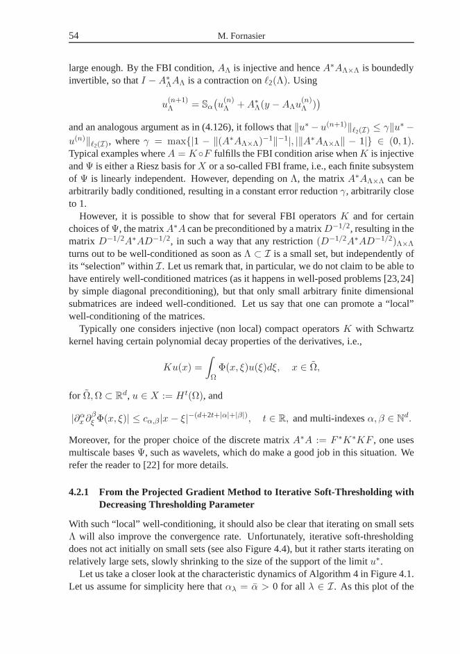
54 M. Fornasier
large enough. By the FBI condition,AΛ is injective and henceA∗AΛ×Λ is boundedlyinvertible, so thatI −A∗
ΛAΛ is a contraction onℓ2(Λ). Using
u(n+1)Λ = Sα
(u
(n)Λ +A∗
Λ(y −AΛu(n)Λ ))
and an analogous argument as in (4.126), it follows that‖u∗ − u(n+1)‖ℓ2(I) ≤ γ‖u∗ −u(n)‖ℓ2(I), whereγ = max|1 − ‖(A∗AΛ×Λ)−1‖−1|, |‖A∗AΛ×Λ‖ − 1| ∈ (0,1).Typical examples whereA = KF fulfills the FBI condition arise whenK is injectiveandΨ is either a Riesz basis forX or a so-called FBI frame, i.e., each finite subsystemof Ψ is linearly independent. However, depending onΛ, the matrixA∗AΛ×Λ can bearbitrarily badly conditioned, resulting in a constant error reductionγ, arbitrarily closeto 1.
However, it is possible to show that for several FBI operators K and for certainchoices ofΨ, the matrixA∗A can be preconditioned by a matrixD−1/2, resulting in thematrixD−1/2A∗AD−1/2, in such a way that any restriction(D−1/2A∗AD−1/2)Λ×Λ
turns out to be well-conditioned as soon asΛ ⊂ I is a small set, but independently ofits “selection” withinI. Let us remark that, in particular, we do not claim to be able tohave entirely well-conditioned matrices (as it happens in well-posed problems [23,24]by simple diagonal preconditioning), but that only small arbitrary finite dimensionalsubmatrices are indeed well-conditioned. Let us say that one can promote a “local”well-conditioning of the matrices.
Typically one considers injective (non local) compact operatorsK with Schwartzkernel having certain polynomial decay properties of the derivatives, i.e.,
Ku(x) =
∫
ΩΦ(x, ξ)u(ξ)dξ, x ∈ Ω,
for Ω,Ω ⊂ Rd, u ∈ X := Ht(Ω), and
|∂αx ∂
βξ Φ(x, ξ)| ≤ cα,β|x− ξ|−(d+2t+|α|+|β|), t ∈ R, and multi-indexesα, β ∈ N
d.
Moreover, for the proper choice of the discrete matrixA∗A := F ∗K∗KF , one usesmultiscale basesΨ, such as wavelets, which do make a good job in this situation.Werefer the reader to [22] for more details.
4.2.1 From the Projected Gradient Method to Iterative Soft-Thresholding withDecreasing Thresholding Parameter
With such “local” well-conditioning, it should also be clear that iterating on small setsΛ will also improve the convergence rate. Unfortunately, iterative soft-thresholdingdoes not act initially on small sets (see also Figure 4.4), but it rather starts iterating onrelatively large sets, slowly shrinking to the size of the support of the limitu∗.
Let us take a closer look at the characteristic dynamics of Algorithm 4 in Figure 4.1.Let us assume for simplicity here thatαλ = α > 0 for all λ ∈ I. As this plot of the
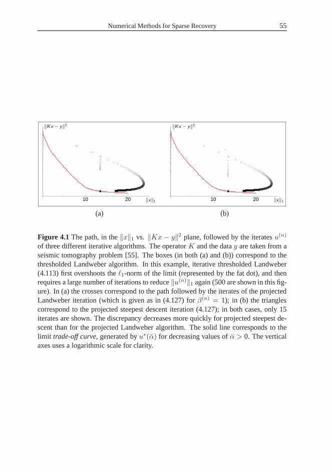
Numerical Methods for Sparse Recovery 55
10 20 10 20
‖Kx − y‖2
‖x‖1
‖Kx − y‖2
‖x‖1
(a) (b)
Figure 4.1 The path, in the‖x‖1 vs. ‖Kx − y‖2 plane, followed by the iteratesu(n)
of three different iterative algorithms. The operatorK and the datay are taken from aseismic tomography problem [55]. The boxes (in both (a) and (b)) correspond to thethresholded Landweber algorithm. In this example, iterative thresholded Landweber(4.113) first overshoots theℓ1-norm of the limit (represented by the fat dot), and thenrequires a large number of iterations to reduce‖u(n)‖1 again (500 are shown in this fig-ure). In (a) the crosses correspond to the path followed by the iterates of the projectedLandweber iteration (which is given as in (4.127) forβ(n) = 1); in (b) the trianglescorrespond to the projected steepest descent iteration (4.127); in both cases, only 15iterates are shown. The discrepancy decreases more quicklyfor projected steepest de-scent than for the projected Landweber algorithm. The solidline corresponds to thelimit trade-off curve, generated byu∗(α) for decreasing values ofα > 0. The verticalaxes uses a logarithmic scale for clarity.
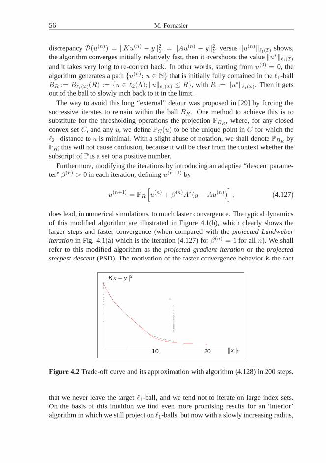
56 M. Fornasier
discrepancyD(u(n)) = ‖Ku(n) − y‖2Y = ‖Au(n) − y‖2
Y versus‖u(n)‖ℓ1(I) shows,the algorithm converges initially relatively fast, then itovershoots the value‖u∗‖ℓ1(I)
and it takes very long to re-correct back. In other words, starting from u(0) = 0, thealgorithm generates a pathu(n); n ∈ N that is initially fully contained in theℓ1-ballBR := Bℓ1(I)(R) := u ∈ ℓ2(Λ); ‖u‖ℓ1(I) ≤ R, with R := ‖u∗‖ℓ1(I). Then it getsout of the ball to slowly inch back to it in the limit.
The way to avoid this long “external” detour was proposed in [29] by forcing thesuccessive iterates to remain within the ballBR. One method to achieve this is tosubstitute for the thresholding operations the projectionPBR
, where, for any closedconvex setC, and anyu, we definePC(u) to be the unique point inC for which theℓ2−distance tou is minimal. With a slight abuse of notation, we shall denotePBR
byPR; this will not cause confusion, because it will be clear fromthe context whether thesubscript ofP is a set or a positive number.
Furthermore, modifying the iterations by introducing an adaptive “descent parame-ter” β(n) > 0 in each iteration, definingu(n+1) by
u(n+1) = PR
[u(n) + β(n)A∗(y −Au(n))
], (4.127)
does lead, in numerical simulations, to much faster convergence. The typical dynamicsof this modified algorithm are illustrated in Figure 4.1(b),which clearly shows thelarger steps and faster convergence (when compared with theprojected Landweberiteration in Fig. 4.1(a) which is the iteration (4.127) forβ(n) = 1 for all n). We shallrefer to this modified algorithm as theprojected gradient iterationor the projectedsteepest descent(PSD). The motivation of the faster convergence behavior isthe fact
10 20
‖Kx − y‖2
‖x‖1
Figure 4.2Trade-off curve and its approximation with algorithm (4.128) in 200 steps.
that we never leave the targetℓ1-ball, and we tend not to iterate on large index sets.On the basis of this intuition we find even more promising results for an ‘interior’algorithm in which we still project onℓ1-balls, but now with a slowly increasing radius,
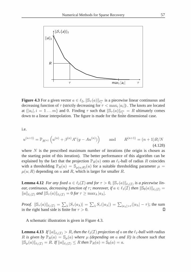
Numerical Methods for Sparse Recovery 57
τ
‖Sτ (a)‖1
‖a‖1
τ
R
maxi |ai |
Figure 4.3For a given vectora ∈ ℓ2, ‖Sτ (a)‖ℓm1
is a piecewise linear continuous anddecreasing function ofτ (strictly decreasing forτ < maxi |ai|) . The knots are locatedat |ai|, i = 1 . . . m and 0. Findingτ such that‖Sτ (a)‖ℓm
1= R ultimately comes
down to a linear interpolation. The figure is made for the finite dimensional case.
i.e.
u(n+1) = PR(n)
(u(n) + β(n)A∗(y −Au(n))
)and R(n+1) = (n+ 1)R/N
(4.128)whereN is the prescribed maximum number of iterations (the origin is chosen asthe starting point of this iteration). The better performance of this algorithm can beexplained by the fact that the projectionPR(u) onto anℓ1-ball of radiusR coincideswith a thresholdingPR(u) = Sµ(u;R)(u) for a suitable thresholding parameterµ =µ(u;R) depending onu andR, which is larger for smallerR.
Lemma 4.12 For any fixeda ∈ ℓ2(I) and forτ > 0, ‖Sτ (a)‖ℓ1(I) is a piecewise lin-ear, continuous, decreasing function ofτ ; moreover, ifa ∈ ℓ1(I) then‖S0(a)‖ℓ1(I) =‖a‖ℓ1(I) and‖Sτ (a)‖ℓ1(I) = 0 for τ ≥ maxλ |aλ|.
Proof. ‖Sτ (a)‖ℓ1(I) =∑
λ |Sτ (aλ)| =∑
λ Sτ (|aλ|) =∑
|aλ|>τ (|aλ| − τ); the sumin the right hand side is finite forτ > 0.
A schematic illustration is given in Figure 4.3.
Lemma 4.13 If ‖a‖ℓ1(I) > R, then theℓ2(I) projection ofa on theℓ1-ball with radiusR is given byPR(a) = Sµ(a) whereµ (depending ona andR) is chosen such that‖Sµ(a)‖ℓ1(I) = R. If ‖a‖ℓ1(I) ≤ R thenPR(a) = S0(a) = a.
58 M. Fornasier
Proof. Suppose‖a‖ℓ1(I) > R. Because, by Lemma 4.12,‖Sµ(a)‖ℓ1(I) is continu-ous inµ and‖Sµ(a)‖ℓ1(I) = 0 for sufficiently largeµ, we can chooseµ such that‖Sµ(a)‖ℓ1(I) = R. (See Figure 4.3.) On the other hand,u∗ = Sµ(a) is the uniqueminimizer of‖u− a‖2
ℓ2(I) + 2µ‖u‖ℓ1(I) (see Lemma 4.1), i.e.,
‖u∗ − a‖2ℓ2(I) + 2µ‖u∗‖ℓ1(I) < ‖u− a‖2
ℓ2(I) + 2µ‖u‖ℓ1(I),
for all u 6= u∗. Since‖u∗‖ℓ1(I) = R, it follows that
for all u ∈ BR, u 6= u∗ : ‖u∗ − a‖2 < ‖u− a‖2
Henceu∗ is closer toa than any otheru inBR. In other words,PR(a) = u∗ = Sµ(a).
This in particular implies that the algorithm (4.128) iterates initially on very smallsets which inflate by growing during the process and approachthe size of the support ofthe target minimizeru∗. Unlike the thresholded Landweber iteration and the projectedsteepest descent [28, 29], unfortunately there is no proof yet of convergence of this‘interior’ algorithm, this being a very interesting open problem.
However, we can provide an algorithm which mimics the behavior of (4.128), i.e., itstarts with large thresholding parametersα(n) and geometrically reduces them duringthe iterations to a target limitα > 0, for which the convergence is guaranteed:
u(n+1) = Sα(n)
[u(n) +A∗y −A∗Au(n)
]. (4.129)
For matricesA for which the restrictionsA∗A|Λ×Λ are uniformly well-conditionedwith respect toΛ of small size, our analysis provides also a prescribed linear rate ofconvergence of the iteration (4.129).
4.2.2 Sample of Analysis of Acceleration Methods
Technical lemmas
We are particularly interested in computing approximations with the smallest possi-ble number of nonzero entries. As a benchmark, we recall thatthe most economicalapproximations of a given vectorv ∈ ℓ2(I) are provided again by thebestk-termapproximationsv[k], defined by discarding inv all but thek ∈ N0 largest coefficientsin absolute value. The error of bestk-term approximation is defined as
σk(v)ℓ2 := ‖v − v[k]‖ℓ2(I). (4.130)
The subspace of allℓ2 vectors with bestk-term approximation rates > 0, i.e.,σk(v)ℓ2 . k−s for some decay rates > 0, is commonly referred to as theweakℓτspaceℓwτ (I), for τ = (s+ 1
2)−1, which, endowed with
|v|ℓwτ (I) := sup
k∈N0
(k + 1)sσk(v)ℓ2, (4.131)
Numerical Methods for Sparse Recovery 59
becomes the quasi-Banach space(ℓwτ (I), | · |ℓwτ (I)). Moreover, for any 0< ǫ ≤ 2− τ ,
we have the continuous embeddingℓτ (I) → ℓwτ (I) → ℓτ+ǫ(I), justifying whyℓwτ (I)is called weakℓτ (I).
When it comes to the concrete computations of good approximations with a smallnumber of active coefficients, one frequently utilizes certain thresholding procedures.Here small entries of a given vector are simply discarded, whereas the large entriesmay be slightly modified. As we have discussed so far, we shallmake use ofsoft-thresholdingthat we have already introduced in (4.114). We recall from Lemma 4.4thatSα is non-expansive for anyα ∈ R
I+,
‖Sα(v) − Sα(w)‖ℓ2(I) ≤ ‖v − w‖ℓ2(I), for all v,w ∈ ℓ2(I). (4.132)
Moreover, for any fixedx ∈ R, the mappingτ 7→ Sτ (x) is Lipschitz continuous and
|Sτ (x) − Sτ ′(x)| ≤ |τ − τ ′|, for all τ, τ ′ ≥ 0. (4.133)
We readily infer the following technical estimate.
Lemma 4.14 Assumev ∈ ℓ2(I), α, β ∈ RI+ such thatα = infλ αλ = infλ βλ = β >
0, and defineΛα(v) :=λ ∈ I : |vλ| > α
. Then
‖Sα(v) − Sβ(v)‖ℓ2(I) ≤(#Λα(v)
)1/2max
λ∈Λα(v)|αλ − βλ|. (4.134)
Proof. It is left as a simple exercise.
Let v ∈ ℓwτ (I), it is well-known [31,§7]
#Λα(v) ≤ C|v|τℓwτ (I)α
−τ , (4.135)
and, forαλ = α for all λ ∈ I, we have
‖v − Sα(v)‖ℓ2(I) ≤ C|v|τ/2ℓwτ (I)α
1−τ/2, (4.136)
where the constants are given byC = C(τ) > 0.In the sequel, we shall also use the following support size estimate.
Lemma 4.15 Let v ∈ ℓwτ (I) andw ∈ ℓ2(I) with ‖v − w‖ℓ2(I) ≤ ǫ. Assumeα =
(αλ)λ∈I ∈ RI+ and infλ αλ = α > 0. Then it holds
# suppSα(w) ≤ #Λα(w) ≤ 4ǫ2
α2 + 4C|v|τℓwτ (I)α
−τ , (4.137)
whereC = C(τ) > 0.
60 M. Fornasier
Proof. We consider two setsI1 = λ ∈ I : |wλ| ≥ α, and|vλ| > α/2, andI2 = λ ∈ I : |wλ| ≥ α, and|vλ| ≤ α/2. Then from (4.135)
#I1 ≤ #λ ∈ I : |vλ| > α/2 ≤ 2τC|v|τℓwτ (I)α
−τ ≤ 4C|v|τℓwτ (I)α
−τ ,
and
(α/2)2(#I2) ≤∑
λ∈I2
|vλ − wλ|2 ≤ ε2.
These estimates imply (4.137).
Decreasing iterative soft-thresholding
For threshold parametersα,α(n) ∈ RI+, whereα(n) ≥ α, i.e.,α(n)
λ ≥ αλ for all λ ∈ Λ,andα = infλ∈I αλ > 0, we consider the iteration
Algorithm 5.
u(0) = 0, u(n+1) = Sα(n)
(u(n) +A∗(y −Au(n))
), n = 0,1, . . . (4.138)
which, forα(n)λ ≥ α
(n+1)λ , we call thedecreasing iterative soft-thresholding algo-
rithm (D-ISTA).
Theorem 4.16 Let ‖A‖ <√
2 and letu := (I − A∗A)u∗ + A∗y ∈ ℓwτ (I) for some
0 < τ < 2. Moreover, letL = L(α) :=4‖u∗‖2
ℓ2(I)
α2 + 4C‖u‖τℓwτ (I)α
−τ , and as-sume that forS∗ := suppu∗ and all finite subsetsΛ ⊂ I with at most#Λ ≤ 2Lelements, the operator(I − A∗A)(S∗∪Λ)×(S∗∪Λ) is contractive onℓ2(S
∗ ∪ Λ), i.e.,‖(I −A∗A)S∗∪Λ×S∗∪Λw‖ℓ2(S∗∪Λ) ≤ γ0‖w‖ℓ2(S∗∪Λ), for all w ∈ ℓ2(S
∗ ∪ Λ), or
‖(I −A∗A)S∗∪Λ×S∗∪Λ‖ ≤ γ0, (4.139)
where0 < γ0 < 1. Then, for anyγ0 < γ < 1, the iteratesu(n) from (4.138)fulfill# suppu(n) ≤ L and they converge tou∗ at a linear rate
‖u∗ − u(n)‖ℓ2(I) ≤ γn‖u∗‖ℓ2(I) =: ǫn (4.140)
whenever theα(n) are chosen according to
αλ ≤ α(n)λ ≤ αλ + (γ − γ0)L
−1/2ǫn, for all λ ∈ Λ. (4.141)
Numerical Methods for Sparse Recovery 61
Proof. We develop the proof by induction. For the initial iterate, we haveu(0) =0, so that# suppu(0) ≤ L and (4.140) is trivially true. Assume as an inductionhypothesis thatS(n) := supp(u(n)) is such that#S(n) ≤ L, and‖u∗ − u(n)‖ℓ2(I) ≤ǫn. Abbreviatingw(n) := u(n) + A∗(y − Au(n)), by ‖A∗A‖ ≤ 2 and the inductionhypothesis, it follows that
‖u−w(n)‖ℓ2(I) =∥∥(I −A∗A)(u∗ − u(n))
∥∥ℓ2(I)
≤ ‖u∗ − u(n)‖ℓ2(I) ≤ ǫn. (4.142)
Hence, using (4.137), we obtain the estimate
#S(n+1) = # supp Sα(n)(w(n)) ≤ Λα(w(n)) ≤ 4ǫ2nα2 +4C|u|τℓw
τ (I)α−τ ≤ L. (4.143)
Since also#S(n) ≤ L by induction hypothesis, the setΛ(n) := S(n) ∪ S(n+1) hasat most 2L elements, so that, by assumption,(I − A∗A)S∪Λ(n)×S∪Λ(n) is contractivewith contraction constantγ0. Using the identities
u∗S∪Λ(n) = Sα(uS∪Λ(n))
= Sα(u∗S∪Λ(n) +A∗
S∪Λ(n)(y −AS∪Λ(n)u∗S∪Λ(n))),
and
u(n+1)S∪Λ(n) = Sα(n)(w
(n)
S∪Λ(n))
= Sα(n)(u(n)
S∪Λ(n) +A∗S∪Λ(n)(y −AS∪Λ(n)u
(n)
S∪Λ(n))),
it follows from (4.132), (4.134), (4.126), andα(n) ≥ α that
‖u∗ − u(n+1)‖ℓ2(I)
= ‖(u∗ − u(n+1))S∪Λ(n)‖ℓ2(S∪Λ(n))
=∥∥Sα(uS∪Λ(n)) − Sα(n)(w
(n)
S∪Λ(n))∥∥
ℓ2(S∪Λ(n))
≤∥∥Sα(uS∪Λ(n)) − Sα(w
(n)
S∪Λ(n))∥∥
ℓ2(S∪Λ(n))
+∥∥Sα(w
(n)
S∪Λ(n)) − Sα(n)(w(n)
S∪Λ(n))∥∥
ℓ2(S∪Λ(n))
≤∥∥(I −A∗A)S∪Λ(n)×S∪Λ(n)(u∗ − u(n))S∪Λ(n)
∥∥ℓ2(S∪Λ(n))
+(#Λα(w(n))
)1/2(max
λ∈Λα(w(n))|αλ − α
(n)λ |)
≤ γ0ǫn +(#Λα(w(n))
)1/2(max
λ∈Λα(w(n))|αλ − α
(n)λ |).
Using (4.143) we obtain‖u−u(n+1)‖ℓ2(I) ≤ γ0ǫn+√L(
maxλ∈Λα(w(n)) |α(n)λ −αλ|
),
and, since theα(n) are chosen according to (4.141), the claim follows.
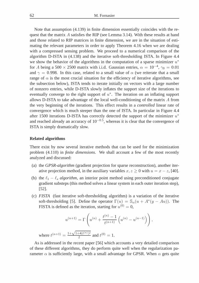
62 M. Fornasier
Note that assumption (4.139) in finite dimension essentially coincides with the re-quest that the matrixA satisfies the RIP (see Lemma 3.14). With these results at handand those related to RIP matrices in finite dimension, we are in the situation of esti-mating the relevant parameters in order to apply Theorem 4.16 when we are dealingwith a compressed sensing problem. We proceed to a numericalcomparison of thealgorithm D-ISTA in (4.138) and the iterative soft-thresholding ISTA. In Figure 4.4we show the behavior of the algorithms in the computation of asparse minimizeru∗
for A being a 500× 2500 matrix with i.i.d. Gaussian entries,α = 10−4, γ0 = 0.01andγ = 0.998. In this case, related to a small value ofα (we reiterate that a smallrange ofα is the most crucial situation for the efficiency of iterativealgorithms, seethe subsection below), ISTA tends to iterate initially on vectors with a large numberof nonzero entries, while D-ISTA slowly inflates the supportsize of the iterations toeventually converge to the right support ofu∗. The iteration on an inflating supportallows D-ISTA to take advantage of the local well-conditioning of the matrixA fromthe very beginning of the iterations. This effect results ina controlled linear rate ofconvergence which is much steeper than the one of ISTA. In particular in Figure 4.4after 1500 iterations D-ISTA has correctly detected the support of the minimizeru∗
and reached already an accuracy of 10−0.5, whereas it is clear that the convergence ofISTA is simply dramatically slow.
Related algorithms
There exist by now several iterative methods that can be usedfor the minimizationproblem (4.110) infinite dimensions. We shall account a few of the most recentlyanalyzed and discussed:
(a) theGPSR-algorithm(gradient projection for sparse reconstruction), anotheriter-ative projection method, in the auxiliary variablesx, z ≥ 0 with u = x− z, [40].
(b) theℓ1 − ℓs algorithm, an interior point method using preconditioned conjugategradient substeps (this method solves a linear system in each outer iteration step),[52].
(c) FISTA (fast iterative soft-thresholding algorithm) is a variation of the iterativesoft-thresholding [5]. Define the operatorΓ(u) = Sα(u + A∗(y − Au)). TheFISTA is defined as the iteration, starting foru(0) = 0,
u(n+1) = Γ
(u(n) +
t(n) − 1
t(n+1)
(u(n) − u(n−1)
)),
wheret(n+1) =1+√
1+4(t(n))2
2 andt(0) = 1.
As is addressed in the recent paper [56] which accounts a verydetailed comparisonof these different algorithms, they do perform quite well when the regularization pa-rameterα is sufficiently large, with a small advantage for GPSR. Whenα gets quite
Numerical Methods for Sparse Recovery 63
0 20 40 60 80 100 120−5
−4
−3
−2
−1
0
1
||un||1
log 10
(||A
un −
y|| 22 )
Dynamics of the algorithms
0 500 1000 1500 2000 2500−3
−2
−1
0
1
2
3Sparse minimizer u* and approximations due to the algorithms
0 200 400 600 800 1000 1200 1400 1600−0.5
0
0.5
1
Number of iterations
log 10
(||u
n − u
* || 2)
Error with respect to the minimizer of J
0 200 400 600 800 1000 1200 1400 16000
0.5
1
1.5
2
2.5
3
3.5
Number of iterations
log 10
(|un | 0)
Dynamics of the support sizes of the approximations to u* due to the algorithms
ISTAD−ISTA
ISTAD−ISTA
ISTAD−ISTA
u*
ISTAD−ISTA
|u*|0
Figure 4.4 We show the behavior of the algorithms ISTA and D-ISTA in the compu-tation of a sparse minimizeru∗ for A being a 500× 2500 matrix with i.i.d. Gaussianentries,α = 10−4, γ0 = 0.01 andγ = 0.998. In the top left figure we present the dy-namics of the algorithms in the plane‖u‖ℓ1 − log(‖Au− y‖2
2). On the bottom left, weshow the absolute error to the precomputed minimizeru∗ with respect to the number ofiterations. On the bottom right we show how the size of the supports of the iterationsgrow with the number of iterations. The figure on the top rightshows the vectoru∗,and the approximations due to the algorithms. In this case D-ISTA detects the rightsupport ofu∗ after 1500 iterations, whereas ISTA keeps dramatically farbehind.
small all the algorithms, except for FISTA, deteriorate significantly their performances.Moreover, local conditioning properties of the linear operatorA seem particularly af-fecting the performances of iterative algorithms.
While these methods are particularly suited for finite dimensional problems, it wouldbe interesting to produce an effective strategy, for any range of the parameterα, fora large class of infinite dimensional problems. In the recentpaper [22] the followingingredients are combined for this scope:
• multiscale preconditioningallows for local well-conditioning of the matrixA andtherefore reproduces at infinite dimension the conditions of best performances foriterative algorithms;
64 M. Fornasier
• adaptivity combined with adecreasing thresholding strategyallow for a con-trolled inflation of the support size of the iterations, promoting the minimal com-putational cost in terms of number of algebraic equations, as well as from thevery beginning of the iteration the exploitation of the local well-conditioning ofthe matrixA.
In [69] the authors propose also an adaptive method similar to [22] where, instead ofthe soft-thresholding, acoarsening function, i.e., a compressed hard-thresholding pro-cedure, is implemented. The emphasis in the latter contribution is on the regularizationproperties of such an adaptive method which does not disposeof a reference energyfunctional (4.108).
5 Large Scale Computing
5.1 Domain Decomposition Methods forℓ1-Minimization
Besides the elegant mathematics needed for the convergenceproof, one of the ma-jor features of Algorithm 4 is its simplicity, also in terms of implementation. Indeedthresholding methods combined with wavelets have been often presented, e.g., in im-age processing, as a possible good alternative to total variation minimization whichrequires instead, as we have already discussed in the previous sections, the solutionof a degenerate partial differential equation. However, aspointed out in the previoussections, in general, iterative soft-thresholding can converge very slowly.
In particular, it is practically not possible to use such algorithm when the dimensionof the problem is really large, unless we provide all the modifications we accountedabove (i.e., preconditioning, decreasing thresholding strategy, adaptivity etc.). Andstill for certain very large scale problems, this might not be enough. For that we needto consider further dimensionality reduction techniques.In this section we introduce asequential domain decomposition method for the linear inverse problem with sparsityconstraints modelled by (4.110). The goal is to join the simplicity of Algorithm 4 witha dimension reduction technique provided by a decomposition which will improve theconvergence and the complexity of the algorithm without increasing the sophisticationof the algorithm.
For simplicity, we start by decomposing the “domain” of the sequencesI into twodisjoint setsI1,I2 so thatI = I1∪I2. The extension to decompositions into multiplesubsetsI = I1 ∪ · · · ∪ IN follows from an analysis similar to the basic caseN = 2.Associated to a decompositionC = I1,I2 we define theextension operatorsEi :ℓ2(Ii) → ℓ2(I), (Eiv)λ = vλ, if λ ∈ Ii, (Eiv)λ = 0, otherwise,i = 1,2. The adjointoperator, which we call therestriction operator, is denoted byRi := E∗
i . With these
Numerical Methods for Sparse Recovery 65
operators we may define the functional,J : ℓ2(I1) × ℓ2(I2) → R, given by
J (u1, u2) := J (E1u1 + E2u2).
For the sequenceui we use the notationuλ,i in order to denote its components. We
want to formulate and analyze the following algorithm: Pickan initial E1u(0)1 +
E2u(0)2 := u(0) ∈ ℓ1(I), for exampleu(0) = 0 and iterate
u(n+1)1 = arg minv1∈ℓ2(I1) J (v1, u
(n)2 )
u(n+1)2 = arg minv2∈ℓ2(I2) J (u
(n+1)1 , v2)
u(n+1) := E1u(n+1)1 + E2u
(n+1)2 .
(5.144)
Let us observe that‖E1u1 + E2u2‖ℓ1(I) = ‖u1‖ℓ1(I1) + ‖u2‖ℓ1(I2), hence
arg minv1∈ℓ2(I1)
J (v1, u(n)2 ) = arg min
v1∈ℓ2(I1)‖(y −AE2u
(n)2 ) −AE1v1‖2
Y + τ‖v1‖ℓ1(I).
A similar formulation holds forarg minv2∈ℓ2(I2) J (u(n+1)1 , v2). This means that the
solution of the local problems onIi is of the samekind as the original problemarg minu∈ℓ2(I) J (u), but the dimension for each has been reduced. Unfortunately
the functionalsJ (u, u(n)2 ) andJ (u
(n+1)1 , v) do not need to have a unique minimizer.
Therefore the formulation as in (5.144) is not in principle well defined. In the follow-ing we will consider a particular choice of the minimizers and in particular we willimplement Algorithm 4 in order to solve each local problem. This choice leads to thefollowing algorithm.
Algorithm 6. Pick an initialE1u(0)1 + E2u
(0)2 := u(0) ∈ ℓ1(I), for example
u(0) = 0, fix L,M ∈ N, and iterate
u(n+1,0)1 = u
(n,L)1
u(n+1,ℓ+1)1 = Sα
(u
(n+1,ℓ)1 +R1A
∗((y −AE2u(n,M)2 ) −AE1u
(n+1,ℓ)1 )
)
ℓ = 0, . . . , L− 1
u(n+1,0)2 = u
(n,M)2
u(n+1,ℓ+1)2 = Sα
(u
(n+1,ℓ)2 +R2A
∗((y −AE1u(n+1,L)1 ) −AE2u
(n+1,ℓ)2 )
)
ℓ = 0, . . . ,M − 1
u(n+1) := E1u(n+1,L)1 +E2u
(n+1,M)2 .
(5.145)
Of course, forL = M = ∞ the previous algorithm realizes a particular instance of(5.144). However, in practice we will never execute an infinite number of inner iter-ations and therefore it is important to analyze the convergence of the algorithm when
66 M. Fornasier
L,M ∈ N are finite.
At this point the question is whether algorithm (5.145) really converges to a mini-mizer of the original functionalJ . This is the scope of the following sections. Onlyfor ease of notation, we assume now that the thresholding parameterα > 0 is a scalar,henceSα(u) acts onu with the same thresholdingSα(uλ) for each vector componentuλ.
5.1.1 Weak Convergence of the Sequential Algorithm
A useful tool in the analysis of non-smooth functionals and their minima is the con-cept of the subdifferential. We shortly introduced it already in the presentation of thehomotopy method in Section 3.1.1. Recall that for a convex functionalF on someBanach spaceV its subdifferential∂F (x) at a pointx ∈ V with F (x) <∞ is definedas the set
∂F (x) = v ∈ V ∗, F (y) − F (x) ≥ v(y − x) for all y ∈ V ,
whereV ∗ denotes the dual space ofV . It is obvious from this definition that 0∈∂F (x) if and only if x is a minimizer ofF .
Example 5.1 Let V = ℓ1(I) andF (x) := ‖x‖ℓ1(I) is theℓ1-norm. We have
∂‖ · ‖ℓ1(I)(x) = ξ ∈ ℓ∞(I) : ξλ ∈ ∂| · |(xλ), λ ∈ I (5.146)
where∂| · |(z) = sgn(z) if z 6= 0 and∂| · |(0) = [−1,1].
By observing that∂(‖A · −y‖2Y )(u) = 2A∗(Au− y) and by an application of [36,
Proposition 5.2] combined with the example above, we obtainthe following charac-terizations of the subdifferentials ofJ andJ S (we recall thatJ S is the surrogatefunctional defined in (4.116)).
Lemma 5.2 i) The subdifferential ofJ at u is given by
∂J (u) = 2A∗(Au− y) + 2α∂‖ · ‖ℓ1(I)(u)
= ξ ∈ ℓ∞(I) : ξλ ∈ [2A∗(Au− y)]λ + 2α∂| · |(uλ).
ii) The subdifferential ofJ S with respect to the sole componentu is given by
∂uJ S(u, a) = −2(a+A∗(y −Aa)) + 2u+ 2α∂‖ · ‖ℓ1(I)(u)
= ξ ∈ ℓ∞(I) : ξλ ∈ [−2(a+A∗(y −Aa))]λ + 2uλ + 2α∂| · |(uλ).
Numerical Methods for Sparse Recovery 67
In light of Lemma 4.2 we can reformulate Algorithm 6 by
u(n+1,0)1 = u
(n,L)1
u(n+1,ℓ+1)1 = arg minu1∈ℓ2(I1) J S(E1u1 + E2u
(n,M)2 , E1u
(n+1,ℓ)1 + E2u
(n,M)2 )
ℓ = 0, . . . , L− 1
u(n+1,0)2 = u
(n,M)2
u(n+1,ℓ+1)2 = arg minu2∈ℓ2(I2) J S(E1u
(n+1,L)1 + E2u2, E1u
(n+1,L)1 + E2u
(n+1,ℓ)2 )
ℓ = 0, . . . ,M − 1
u(n+1) := E1u(n+1,L)1 + E2u
(n+1,M)2 .
(5.147)Before we actually start proving the weak convergence of thealgorithm in (5.147) werecall the following definition [71].
Definition 5.3 Let V be a topological space andA = (An)n∈N a sequence of subsetsof V . The subsetA ⊆ V is called thelimit of the sequenceA, and we writeA =limnAn, if
A = a ∈ V : ∃an ∈ An, a = limnan.
The following observation will be useful to us, see, e.g., [71, Proposition 8.7].
Lemma 5.4 Assume thatΓ is a convex function onRM and (xn)n∈N ⊂ RM a con-
vergent sequence with limitx such thatΓ(xn),Γ(x) < ∞. Then the subdifferentialssatisfy
limn→∞
∂Γ(xn) ⊆ ∂Γ(x).
In other words, the subdifferential∂Γ of a convex function is anouter semicontinuousset-valued function.
Theorem 5.5 (Weak convergence)The algorithm in(5.147)produces a sequence(u(n))n∈N
in ℓ2(I) whose weak accumulation points are minimizers of the functionalJ . In par-ticular, the set of the weak accumulation points is non-empty and ifu(∞) is a weakaccumulation point then
u(∞) = Sα(u(∞) +A∗(g −Au(∞))).
Proof. The proof is partially inspired by the one of Theorem 3.12, where also alter-nating minimizations were considered. Let us first observe that by (4.118)
J (u(n)) = J S(u(n), u(n)) = J S(E1u(n,L)1 + E2u
(n,M)2 , E1u
(n,L)1 + E2u
(n,M)2 )
= J S(E1u(n,L)1 + E2u
(n,M)2 , E1u
(n+1,0)1 + E2u
(n,M)2 ).
68 M. Fornasier
By definition ofu(n+1,1)1 and its minimal properties in (5.147) we have
J S(E1u(n,L)1 + E2u
(n,M)2 , E1u
(n+1,0)1 + E2u
(n,M)2 )
≥ J S(E1u(n+1,1)1 + E2u
(n,M)2 , E1u
(n+1,0)1 + E2u
(n,M)2 ).
Again, an application of (4.118) gives
J S(E1u(n+1,1)1 + E2u
(n,M)2 , E1u
(n+1,0)1 + E2u
(n,M)2 )
≥ J S(E1u(n+1,1)1 + E2u
(n,M)2 , E1u
(n+1,1)1 + E2u
(n,M)2 ).
Concatenating these inequalities we obtain
J (u(n)) ≥ J S(E1u(n+1,1)1 + E2u
(n,M)2 , E1u
(n+1,1)1 + E2u
(n,M)2 ).
In particular, from (4.119) we have
J (u(n)) − J S(E1u(n+1,1)1 + E2u
(n,M)2 , E1u
(n+1,1)1 + E2u
(n,M)2 )
≥ C‖u(n+1,1)1 − u
(n+1,0)1 ‖2
ℓ2(I1).
By induction we obtain
J (u(n)) ≥ J S(E1u(n+1,1)1 + E2u
(n,M)2 , E1u
(n+1,1)1 + E2u
(n,M)2 ) ≥ . . .
≥ J S(E1u(n+1,L)1 + E2u
(n,M)2 , E1u
(n+1,L)1 + E2u
(n,M)2 )
= J (E1u(n+1,L)1 + E2u
(n,M)2 ),
and
J (u(n)) − J (E1u(n+1,L)1 + E2u
(n,M)2 ) ≥ C
L−1∑
ℓ=0
‖u(n+1,ℓ+1)1 − u
(n+1,ℓ)1 ‖2
ℓ2(I1).
By definition ofu(n+1,1)2 and its minimal properties we have
J S(E1u(n+1,L)1 + E2u
(n,M)2 , E1u
(n+1,L)1 + E2u
(n,M)2 )
≥ J S(E1u(n+1,L)1 + E2u
(n+1,1)2 , E1u
(n+1,L)1 + E2u
(n+1,0)2 ).
By similar arguments as above we find
J (u(n)) ≥ J S(E1u(n+1,L)1 +E2u
(n+1,M)2 , E1u
(n+1,L)1 +E2u
(n+1,M)2 ) = J (u(n+1)),
(5.148)
Numerical Methods for Sparse Recovery 69
and
J (u(n)) − J (u(n+1))
≥ C
(L−1∑
ℓ=0
‖u(n+1,ℓ+1)1 − u
(n+1,ℓ)1 ‖2
ℓ2(I1)+
M−1∑
m=0
‖u(n+1,m+1)2 − u
(n+1,m)2 ‖2
ℓ2(I2)
).
(5.149)
From (5.148) we haveJ (u(0)) ≥ J (u(n)) ≥ 2α‖u(n)‖ℓ1(I) ≥ 2α‖u(n)‖ℓ2(I). Thismeans that(u(n))n∈N is uniformly bounded inℓ2(I), hence there exists a weakly con-vergent subsequence(u(nj))j∈N. Let us denoteu(∞) the weak limit of the subse-quence. For simplicity, we rename such subsequence by(u(n))n∈N. Moreover, sincethe sequence(J (u(n)))n∈N is monotonically decreasing and bounded from below by0, it is also convergent. From (5.149) and the latter convergence we deduce
(L−1∑
ℓ=0
‖u(n+1,ℓ+1)1 − u
(n+1,ℓ)1 ‖2
ℓ2(I1)+
M−1∑
m=0
‖u(n+1,m+1)2 − u
(n+1,m)2 ‖2
ℓ2(I2)
)→ 0,
(5.150)for n→ ∞. In particular, by the standard inequality(a2+b2) ≥ 1
2(a+b)2 for a, b > 0and the triangle inequality, we have also
‖u(n) − u(n+1)‖ℓ2(I) → 0, n→ ∞. (5.151)
We would like to show now that
0 ∈ limn→∞
∂J (u(n)) ⊂ ∂J (u(∞)).
To this end, and in light of Lemma 5.2, we reason componentwise. By definition ofu
(n+1,L)1 we have
0 ∈ [−2(u(n+1,L−1)1 +R1A
∗((y −AE2u(n,M)2 ) −AE1u
(n+1,L−1)1 ))]λ
+ 2u(n+1,L)λ,1 + 2α∂| · |(u(n+1,L)
λ,1 ), (5.152)
for λ ∈ I1, and by definition ofu(n+1,M)2 we have
0 ∈ [−2(u(n+1,M−1)2 +R2A
∗((y −AE1u(n+1,L)1 ) −AE2u
(n+1,M−1)2 ))]λ
+ 2u(n+1,M)λ,2 + 2α∂| · |(u(n+1,M)
λ,2 ), (5.153)
for λ ∈ I2. Let us compute∂J (u(n+1))λ,
∂J (u(n+1))λ = [−2A∗(y −AE1u(n+1,L)1 −AE2u
(n+1,M)2 )]λ + 2α∂| · |(u(n+1,K)
λ,i ),(5.154)
70 M. Fornasier
whereλ ∈ Ii andK = L,M for i = 1,2 respectively. We would like to find aξ(n+1)λ ∈ ∂J (u(n+1))λ such thatξ(n+1)
λ → 0 for n→ ∞. By (5.152) we have that forλ ∈ I1
0 = [−2(u(n+1,L−1)1 +R1A
∗((y −AE2u(n,M)2 ) −AE1u
(n+1,L−1)1 ))]λ
+ 2u(n+1,L)λ,1 + 2αξ(n+1)
λ,1 ,
for a ξ(n+1)λ,1 ∈ ∂| · |(u(n+1,L)
λ,1 ), and, by (5.153), forλ ∈ I2
0 = [−2(u(n+1,M−1)2 +R2A
∗((y −AE1u(n+1,L)1 ) −AE2u
(n+1,M−1)2 ))]λ
+ 2u(n+1,M)λ,2 + 2αξ(n+1)
λ,2 ,
for a ξ(n+1)λ,2 ∈ ∂| · |(u(n+1,M)
λ,2 ). Thus by adding zero to (5.154) as represented by theprevious two formulas, we can choose
ξ(n+1)λ = 2(u
(n+1,L)λ,1 − u
(n+1,L−1)λ,1 ) + [R1A
∗AE1(u(n+1,L)1 − u
(n+1,L−1)1 )]λ
+ [R1A∗AE2(u
(n+1,M)2 − u
(n,M)1 )]λ,
if λ ∈ I1 and
ξ(n+1)λ = 2(u
(n+1,M)λ,2 − u
(n+1,M−1)λ,2 ) + [R2A
∗AE1(u(n+1,M)2 − u
(n+1,M−1)1 )]λ,
if λ ∈ I2. For both these choices, from (5.150) and (5.151), and by continuity of A,we haveξ(n+1)
λ → 0 for n→ ∞. Again by continuity ofA, weak convergence ofu(n)
(which implies componentwise convergence), and Lemma 5.4 we obtain
0 ∈ limn→∞
∂J (u(n))λ ⊂ ∂J (u(∞)λ, for all λ ∈ I.
It follows from Lemma 5.2 that 0∈ ∂J (u(∞). By the properties of the subdifferen-tial we have thatu(∞) is a minimizer ofJ . Of course, the reasoning above holds forany weakly convergent subsequence and therefore all weak accumulation points of theoriginal sequence(u(n))n are minimizers ofJ .
Similarly, by taking now the limit forn → ∞ in (5.152) and (5.153), and by using(5.150) we obtain
0 ∈ [−2(R1u(∞)+R1A
∗((y−AE2R2u(∞))−AE1R1u
(∞)))]λ+2u(∞)λ +2α∂|·|(u(∞)
λ ),
for λ ∈ I1 and
0 ∈ [−2(R2u(∞)+R2A
∗((y−AE1R1u(∞)−AE2R2u
(∞))]λ+2u(∞)λ +2α∂|·|(u(∞)
λ ).
Numerical Methods for Sparse Recovery 71
for λ ∈ I2. In other words, we have
0 ∈ ∂uJ S(u(∞), u(∞)).
An application of Lemma 5.2 and Proposition 4.5 imply
u(∞) = Sα(u(∞) +A∗(y −Au(∞))).
Remark 5.6 1. Becauseu(∞) = Sα(u(∞) + A∗(y − Au(∞))), we could infer theminimality of u(∞) by invoking Proposition 4.5. In the previous proof we wantedtopresent an alternative argument based on differential inclusions.
2. Since(u(n))n∈N is bounded and (5.150) holds, also(un,ℓi )n,ℓ are bounded for
i = 1,2.
5.1.2 Strong Convergence of the Sequential Algorithm
In this section we want to show that the convergence of a subsequence(unj )j to anyaccumulation pointu(∞) holds not only in the weak topology, but also in the Hilbertspaceℓ2(I) norm. Let us define
η(n+1) := u(n+1,L)1 − u
(∞)1 , η(n+1/2) := u
(n+1,L−1)1 − u
(∞)1 ,
µ(n+1) := u(n+1,M)2 − u
(∞)2 , µ(n+1/2) := u
(n+1,M−1)2 − u
(∞)2 ,
whereu(∞)i := Riu
(∞). From Theorem 5.5 we also have
u(∞)i = Sα(u
(∞)i +RiA
∗(y −AE1u(∞)1 −AE2u
(∞)2 )︸ ︷︷ ︸
:=hi
), i = 1,2.
Let us also denoteh := E1h1 + E2h2 andξ(n) := E1η(n+1/2) + E2µ
(n+1/2).
For the proof of strong convergence we need the following technical lemmas. Thestrategy of their proofs is similar to that of Lemma 4.8 and Lemma 4.9.
Lemma 5.7 ‖Aξ(n)‖2Y → 0 for n→ ∞.
Proof. Since
η(n+1) − η(n+1/2) = Sα(h1 + (I −R1A∗AE1)η
(n+1/2)
− R1A∗AE2µ
(n)) − Sα(h1) − η(n+1/2),
µ(n+1) − µ(n+1/2) = Sα(h2 + (I −R2A∗AE2)µ
(n+1/2)
− R2A∗AE1η
(n+1)) − Sα(h2) − µ(n+1/2),
72 M. Fornasier
and ‖η(n+1) − η(n+1/2)‖ℓ2(I1) = ‖u(n+1,L)1 − u
(n+1,L−1)1 ‖ℓ2(I1) → 0, ‖µ(n+1) −
µ(n+1/2)‖ℓ2(I1) = ‖u(n+1,M)2 − u
(n+1,M−1)2 ‖ℓ2(I2) → 0 by (5.150), we have
‖Sα(h1 + (I −R1A∗AE1)η
(n+1/2) −R1A∗AE2µ
(n)) − Sα(h1) − η(n+1/2)‖ℓ2(I1)
≥∣∣∣‖Sα(h1 + (I −R1A
∗AE1)η(n+1/2) −R1A
∗AE2µ(n))
−Sα(h1)‖ℓ2(I1) − ‖η(n+1/2)‖ℓ2(I1)
∣∣∣→ 0, (5.155)
and
‖Sα(h2 + (I −R2A∗AE2)µ
(n+1/2) −R2A∗AE1η
(n+1)) − Sα(h2) − µ(n+1/2)‖ℓ2(I2)
≥∣∣∣‖Sα(h2 + (I −R2A
∗AE2)µ(n+1/2) −R2A
∗AE1η(n+1))
−Sα(h2)‖ℓ2(I2) − ‖µ(n+1/2)‖ℓ2(I2)
∣∣∣→ 0. (5.156)
By nonexpansiveness ofSα we have the estimates
‖Sα(h2 + (I −R2A∗AE2)µ
(n+1/2) −R2A∗AE1η
(n+1)) − Sα(h2)‖ℓ2(I2)
≤ ‖(I −R2A∗AE2)µ
(n+1/2) −R2A∗AE1η
(n+1)‖ℓ2(I2)
≤ ‖(I −R2A∗AE2)µ
(n+1/2) −R2A∗AE1η
(n+1/2)‖ℓ2(I2)
+ ‖R2A∗AE1(η
(n+1/2)) − η(n+1))‖ℓ2(I2)︸ ︷︷ ︸:=ε(n)
.
Similarly, we have
‖Sα(h1 + (I −R1A∗AE1)η
(n+1/2) −R1A∗AE2µ
(n)) − Sα(h1)‖ℓ2(I1)
≤ ‖(I −R1A∗AE1)η
(n+1/2) −R1A∗AE2µ
(n)‖ℓ2(I1)
≤ ‖(I −R1A∗AE1)η
(n+1/2) −R1A∗AE2µ
(n+1/2)‖ℓ2(I1)
+ ‖R1A∗AE2(µ
(n+1/2) − µ(n))‖ℓ2(I1)︸ ︷︷ ︸δ(n)
.
Numerical Methods for Sparse Recovery 73
Combining the previous inequalities, we obtain the estimates
‖Sα(h1 + (I −R1A∗AE1)η
(n+1/2) −R1A∗AE2µ
(n) − Sα(h1)‖2ℓ2(I1)
+ ‖Sα(h2 + (I −R2A∗AE2)µ
(n+1/2) −R2A∗AE1η
(n+1) − Sα(h2)‖2ℓ2(I2)
≤ ‖(I −R1A∗AE1)η
(n+1/2) −R1A∗AE2µ
(n)‖2ℓ2(I1)
+ ‖(I −R2A∗AE2)µ
(n+1/2) −R2A∗AE1η
(n+1)‖2ℓ2(I2)
=(‖(I −R1A
∗AE1)η(n+1/2) −R1A
∗AE2µ(n+1/2)‖ℓ2(I1)
+ ‖R1A∗AE2(µ
(n+1/2) − µ(n))‖ℓ2(I1)
)2
+(‖(I −R2A
∗AE2)µ(n+1/2) −R2A
∗AE1η(n+1/2)‖ℓ2(I2)
+ ‖R2A∗AE1(η
(n+1/2)) − η(n+1)‖ℓ2(I2)
)2
≤ ‖(I −A∗A)ξ(n)‖2ℓ2(I) + ((ε(n))2 + (δ(n))2 + C ′(ε(n) + δ(n)))
≤ ‖ξ(n)‖2ℓ2(I) + ((ε(n))2 + (δ(n))2 + C ′(ε(n) + δ(n)))
The constantC ′ > 0 is due to the boundedness ofu(n,ℓ). Certainly, by (5.150), foreveryε > 0 there existsn0 such that forn > n0 we have(ε(n))2 +(δ(n))2 +C ′(ε(n) +δ(n))) ≤ ε. Therefore, if
‖Sα(h1 + (I −R1A∗AE1)η
(n+1/2) −R1A∗AE2µ
(n) − Sα(h1)‖2ℓ2(I1)
+ ‖Sα(h2 + (I −R2A∗AE2)µ
(n+1/2) −R2A∗AE1η
(n+1) − Sα(h2)‖2ℓ2(I2)
≥ ‖ξ(n)‖2ℓ2(I),
then
0 ≤ ‖(I −R1A∗AE1)µ
(n+1/2) −R1A∗AE2µ
(n)‖2ℓ2(I1)
+ ‖(I −R2A∗AE2)µ
(n+1/2) −R2A∗AE1η
(n+1)‖2ℓ2(I) − ‖ξ(n)‖2
ℓ2(I)
≤ (ε(n))2 + (δ(n))2 + C ′(ε(n) + δ(n))) ≤ ε
If, instead, we have
‖Sα(h1 + (I −R1A∗AE1)η
(n+1/2) −R1A∗AE2µ
(n)) − Sα(h1)‖2ℓ2(I1)
+ ‖Sα(h2 + (I −R2A∗AE2)µ
(n+1/2) −R2A∗AE1η
(n+1)) − Sα(h2)‖2ℓ2(I2)
< ‖ξ(n)‖2ℓ2(I),
74 M. Fornasier
then by (5.155) and (5.156)
‖ξ(n)‖2ℓ2(I) −
(‖(I −R1A
∗AE1)µ(n+1/2) −R1A
∗AE2µ(n))‖2
ℓ2(I1)
+ ‖(I −R2A∗AE2)µ
(n+1/2) −R2A∗AE1η
(n+1))‖2ℓ2(I2)
)
≤ ‖ξ(n)‖2ℓ2(I)
− ‖Sα(h1 + (I −R1A∗AE1)η
(n+1/2) −R1A∗AE2µ
(n)) − Sα(h1)‖2ℓ2(I1)
− ‖Sα(h2 + (I −R2A∗AE2)µ
(n+1/2) −R2A∗AE1η
(n+1)) − Sα(h2)‖2ℓ2(I2)
=∣∣∣‖ξ(n)‖2
ℓ2(I)
− ‖Sα(h1 + (I −R1A∗AE1)η
(n+1/2) −R1A∗AE2µ
(n)) − Sα(h1)‖2ℓ2(I1)
− ‖Sα(h2 + (I −R2A∗AE2)µ
(n+1/2) −R2A∗AE1η
(n+1)) − Sα(h2)‖2ℓ2(I2)
∣∣∣
≤∣∣∣‖η(n+1/2)‖2
ℓ2(I1)
− ‖Sα(h1 + (I −R1A∗AE1)η
(n+1/2) −R1A∗AE2µ
(n)) − Sα(h1)‖2ℓ2(I1)
∣∣∣
+∣∣∣‖µ(n+1/2)‖2
ℓ2(I2)
− ‖Sα(h2 + (I −R2A∗AE2)µ
(n+1/2) −R2A∗AE1η
(n+1)) − Sα(h2)‖2ℓ2(I2)
∣∣∣ ≤ ε
for n large enough. This implies
limn→∞
[‖ξ(n)‖2
ℓ2(I) −(‖(I −R1A
∗AE1)µ(n+1/2) −R1A
∗AE2µ(n)‖2
ℓ2(I1)
+ ‖(I −R2A∗AE2)µ
(n+1/2) −R2A∗AE1η
(n+1)‖2ℓ2(I2)
)]= 0.
Observe now that
‖(I −R1A∗AE1)µ
(n+1/2) −R1A∗AE2µ
(n)‖2ℓ2(I1)
+ ‖(I −R2A∗AE2)µ
(n+1/2) −R2A∗AE1η
(n+1)‖2ℓ2(I2)
≤ (‖(I −R1A∗AE1)µ
(n+1/2) −R1A∗AE2µ
(n+1/2)‖ℓ2(I1) + δ(n))2
+ (‖(I −R2A∗AE2)µ
(n+1/2) −R2A∗AE1η
(n+1/2)‖ℓ2(I2) + ε(n))2
≤ ‖(I −A∗A)ξ(n)‖2ℓ2(I) +
((ε(n))2 + (δ(n))2 + 2C ′(ε(n) + δ(n))
),
Numerical Methods for Sparse Recovery 75
for a suitable constantC ′ > 0 as above. Therefore we have
‖ξ(n)‖2ℓ2(I) −
(‖(I −R1A
∗AE1)µ(n+1/2) −R1A
∗AE2µ(n))‖2
ℓ2(I1)
+ ‖(I −R2A∗AE2)µ
(n+1/2) −R2A∗AE1η
(n+1))‖2ℓ2(I2)
)
≥ ‖ξ(n)‖2ℓ2(I) − ‖(I −A∗A)ξ(n)‖2
ℓ2(I) −((ε(n))2 + (δ(n))2 + 2C ′(ε(n) + δ(n))
)
= 2‖Aξ(n)‖2Y − ‖A∗Aξ(n)‖2
ℓ2(I) −((ε(n))2 + (δ(n))2 + 2C ′(ε(n) + δ(n))
)
≥ ‖Aξ(n)‖2Y −
((ε(n))2 + (δ(n))2 + 2C ′(ε(n) + δ(n))
).
This implies‖Aξ(n)‖2Y → 0 for n→ ∞.
Lemma 5.8 For h = E1h1 + E2h2, ‖Sα(h + ξ(n)) − Sα(h) − ξ(n)‖ℓ2(I) → 0, forn→ ∞.
Proof. We have
Sα(h+ ξ(n) −A∗Aξ(n))
= E1
(Sα(h1 + (I −R1A
∗AE1)η(n+1/2) −R1A
∗AE2µ(n+1/2))
)
+ E2
(Sα(h2 + (I −R2A
∗AE2)µ(n+1/2) −R2A
∗AE1η(n+1/2))
)
Therefore, we can write
Sα(h+ ξ(n) −A∗Aξ(n))
= E1
[Sα(h1 + (I −R1A
∗AE1)η(n+1/2) −R1A
∗AE2µ(n))
+ Sα(h1 + (I −R1A∗AE1)η
(n+1/2) −R1A∗AE2µ
(n+1/2))
− Sα(h1 + (I −R1A∗AE1)η
(n+1/2) −R1A∗AE2µ
(n))]
+ E2
[Sα(h2 + (I −R2A
∗AE2)µ(n+1/2) −R2A
∗AE1η(n+1))
+ Sα(h2 + (I −R2A∗AE2)µ
(n+1/2) −R2A∗AE1η
(n+1/2))
− Sα(h2 + (I −R2A∗AE2)µ
(n+1/2) −R2A∗AE1η
(n+1))].
By using the nonexpansiveness ofSα, the boundedness of the operatorsEi, Ri, A∗A,
76 M. Fornasier
and the triangle inequality we obtain,
‖Sα(h+ ξ(n)) − Sα(h) − ξ(n)‖ℓ2(I)
≤ ‖Sα(h+ ξ(n) −A∗Aξ(n)) − Sα(h) − ξ(n)‖ℓ2(I)
+ ‖Sα(h+ ξ(n)) − Sα(h+ ξ(n) −A∗Aξ(n))‖ℓ2(I)
≤‖Sα(h1 + (I −R1A
∗AE1)η(n+1/2) −R1A
∗AE2µ(n)) − Sα(h1) − η(n+1/2)‖ℓ2(I1)︸ ︷︷ ︸
:=A(n)
+ ‖Sα(h2 + (I −R2A∗AE2)µ
(n+1/2) −R2A∗AE1η
(n+1)) − Sα(h2) − µ(n+1/2)‖ℓ2(I2)︸ ︷︷ ︸:=B(n)
+ ‖µ(n+1/2) − µ(n)‖ℓ2(I2) + ‖η(n+1) − η(n+1/2)‖ℓ2(I1)︸ ︷︷ ︸:=C(n)
+ ‖A∗Aξ(n)‖ℓ2(I)︸ ︷︷ ︸:=D(n)
.
The quantitiesA(n), B(n) vanish forn → ∞ because of (5.155) and (5.156). ThequantityC(n) vanishes forn→ ∞ because of (5.150), andD(n) vanishes forn→ ∞thanks to Lemma 5.7.
By combining the previous technical achievements, we can now state the strongconvergence.
Theorem 5.9 (Strong convergence)Algorithm 6 produces a sequence(u(n))n∈N inℓ2(I) whose strong accumulation points are minimizers of the functional J . In par-ticular, the set of strong accumulation points is non-empty.
Proof. Let u(∞) be a weak accumulation point and let(u(nj))j∈N be a subsequenceweakly convergent tou(∞). Let us again denote the latter sequence(u(n))n∈N. Withthe notation used in this section, by Theorem 5.5 and (5.150)we have thatξ(n) =E1η
(n+1/2) + E2µ(n+1/2) weakly converges to zero. By Lemma 5.8 we have
limn→∞
‖Sα(h+ ξ(n)) − Sα(h) − ξ(n)‖ℓ2(I) = 0.
From Lemma 4.10 we conclude thatξ(n) = E1η(n+1/2) + E2µ
(n+1/2) converges tozero strongly. Again by (5.150) we have that(u(n))n∈N converges tou(∞) strongly.
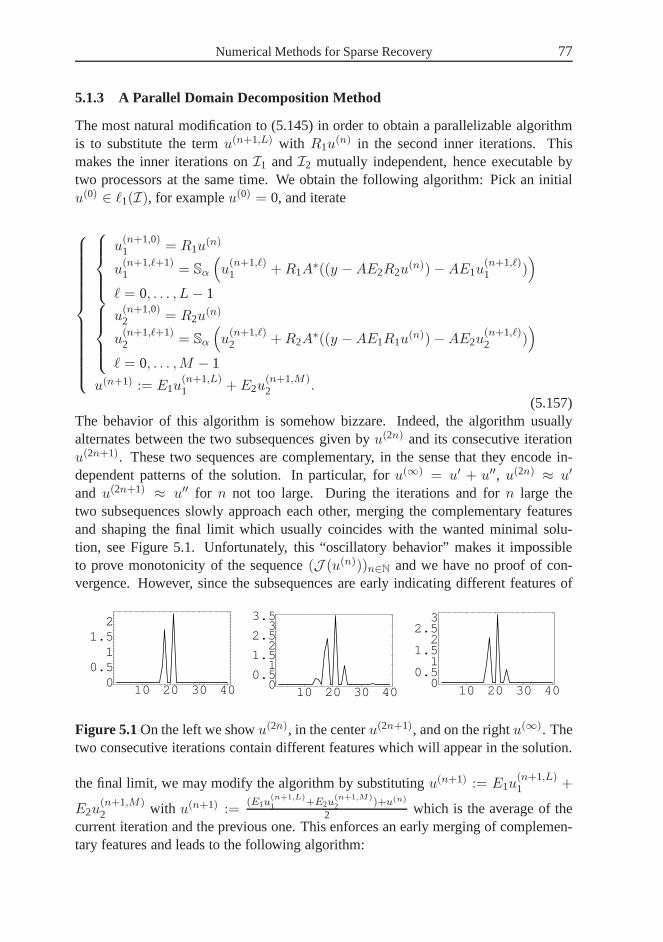
Numerical Methods for Sparse Recovery 77
5.1.3 A Parallel Domain Decomposition Method
The most natural modification to (5.145) in order to obtain a parallelizable algorithmis to substitute the termu(n+1,L) with R1u
(n) in the second inner iterations. Thismakes the inner iterations onI1 andI2 mutually independent, hence executable bytwo processors at the same time. We obtain the following algorithm: Pick an initialu(0) ∈ ℓ1(I), for exampleu(0) = 0, and iterate
u(n+1,0)1 = R1u
(n)
u(n+1,ℓ+1)1 = Sα
(u
(n+1,ℓ)1 +R1A
∗((y −AE2R2u(n)) −AE1u
(n+1,ℓ)1 )
)
ℓ = 0, . . . , L− 1
u(n+1,0)2 = R2u
(n)
u(n+1,ℓ+1)2 = Sα
(u
(n+1,ℓ)2 +R2A
∗((y −AE1R1u(n)) −AE2u
(n+1,ℓ)2 )
)
ℓ = 0, . . . ,M − 1
u(n+1) := E1u(n+1,L)1 + E2u
(n+1,M)2 .
(5.157)The behavior of this algorithm is somehow bizzare. Indeed, the algorithm usuallyalternates between the two subsequences given byu(2n) and its consecutive iterationu(2n+1). These two sequences are complementary, in the sense that they encode in-dependent patterns of the solution. In particular, foru(∞) = u′ + u′′, u(2n) ≈ u′
and u(2n+1) ≈ u′′ for n not too large. During the iterations and forn large thetwo subsequences slowly approach each other, merging the complementary featuresand shaping the final limit which usually coincides with the wanted minimal solu-tion, see Figure 5.1. Unfortunately, this “oscillatory behavior” makes it impossibleto prove monotonicity of the sequence(J (u(n)))n∈N and we have no proof of con-vergence. However, since the subsequences are early indicating different features of
10 20 30 400
0.51
1.52
10 20 30 400
0.51
1.52
2.53
3.5
10 20 30 400
0.51
1.52
2.53
Figure 5.1On the left we showu(2n), in the centeru(2n+1), and on the rightu(∞). Thetwo consecutive iterations contain different features which will appear in the solution.
the final limit, we may modify the algorithm by substitutingu(n+1) := E1u(n+1,L)1 +
E2u(n+1,M)2 with u(n+1) :=
(E1u(n+1,L)1 +E2u
(n+1,M)2 )+u(n)
2 which is the average of thecurrent iteration and the previous one. This enforces an early merging of complemen-tary features and leads to the following algorithm:
78 M. Fornasier
Algorithm 7. Pick an initialu(0) ∈ ℓ1(I), for exampleu(0) = 0, and iterate
u(n+1,0)1 = R1u
(n)
u(n+1,ℓ+1)1 = Sα
(u
(n+1,ℓ)1 +R1A
∗((y −AE2R2u(n)) −AE1u
(n+1,ℓ)1 )
)
ℓ = 0, . . . , L− 1
u(n+1,0)2 = R2u
(n)
u(n+1,ℓ+1)2 = Sα
(u
(n+1,ℓ)2 +R2A
∗((y −AE1R1u(n)) −AE2u
(n+1,ℓ)2 )
)
ℓ = 0, . . . ,M − 1
u(n+1) :=(E1u
(n+1,L)1 +E2u
(n+1,M)2 )+u(n)
2 .(5.158)
The proof of strong convergence of this algorithm is very similar to the one ofAlgorithm 6. For the details, we refer the reader to [42].
5.2 Domain Decomposition Methods for Total Variation Minimization
We would like to continue here our parallel discussion ofℓ1-minimization and totalvariation minimization as we did in Section 3.1.3. In particular, we would like to showthat also for total variation minimization it is possible toformulate domain decompo-sition methods. Several numerical strategies to efficiently perform total variation mini-mization have been proposed in the literature as well [2,14,15,17,21,26,68,81,83]. Inparticular in Section 3.1.3 we mentioned specifically the linearization approach by it-eratively least squares presented in [16,32]. These approaches differ significantly, andthey provide a convincing view of the interest this problem has been able to generateand of its applicative impact. However, because of their iterative-sequential formula-tion, none of the mentioned methods is able to address extremely large problems, suchas 4D imaging (spatial plus temporal dimensions) from functional magnetic-resonancein nuclear medical imaging, astronomical imaging or globalterrestrial seismic tomog-raphy, in real-time, or at least in an acceptable computational time. For such large scalesimulations we need to address methods which allow us to reduce the problem to a fi-nite sequence of sub-problems of a more manageable size, perhaps computable by oneof the methods listed above. We address the interested reader to the broad literatureincluded in [45] for an introduction to domain decomposition methods both for PDEsand convex minimization. This section will make use of more advanced concepts andresults in convex analysis, which we will not introduce, andwe refer the interestedreader to the books [36,50].
Numerical Methods for Sparse Recovery 79
Difficulty of the problem
Due to the nonsmoothness and nonadditivity of the total variation with respect to anonoverlapping domain decomposition (note that the total variation of a function onthe whole domain equals the sum of the total variations on thesubdomains plus thesize of the jumps at the interfaces [45, formula (3.4)]; thisis one of the main dif-ferences to the situation we already encountered withℓ1-minimization), one encoun-ters additional difficulties in showing convergence of suchdecomposition strategies toglobal minimizers. In particular, we stress very clearly that well-known approachesas in [13, 18, 79, 80] are not directly applicable to this problem, because either theyaddress additive problems (as the one ofℓ1-minimization) or smooth convex mini-mizations, which isnot the case of total variation minimization. We emphasize thatthe successful convergence of such alternating algorithmsis far from being obvious fornonsmooth and nonadditive problems, as many counterexamples can be constructed,see for instance [82].
The approach, results, and technical issues
In this section we show how to adapt Algorithm 6 and Algorithm7 to the case ofan overlappingdomain decomposition for total variation minimization. The settingof an overlapping domain decomposition eventually provides us with a frameworkin which one can successfully prove its convergence to minimizers ofJ in (3.82),both in its sequential and parallel forms. Let us stress thatto our knowledge this isthe first method which addresses a domain decomposition strategy for total variationminimization with a formal, theoretical justification of convergence [45,60,84].
The analysis below is performed again for the discrete approximation of the contin-uous functional (3.81), for ease again denotedJ in (3.82). Essentially we approximatefunctionsu by their sampling on a regular grid and their gradientDu by finite differ-ences∇u. For ease of presentation, and in order to avoid unnecessarytechnicalities,we limit our analysis to splitting the problem into two subdomainsΩ1 andΩ2. This isby no means a restriction. The generalization to multiple domains comes quite naturalin our specific setting, see also [45, Remark 5.3]. When dealing with discrete subdo-mainsΩi, for technical reasons, we will require a certain splittingproperty for the totalvariation, i.e.,
|∇u|(Ω) = |∇u|Ω1|(Ω1) + c1(u|(Ω2\Ω1)∪Γ1),
|∇u|(Ω) = |∇u|Ω2|(Ω2) + c2(u|(Ω1\Ω2)∪Γ2), (5.159)
wherec1 andc2 are suitable functions which depend only on the restrictionsu|(Ω2\Ω1)∪Γ1
andu|(Ω1\Ω2)∪Γ2respectively, see (5.166) (symbols and notations are thoseintroduced
in Section 3.1.3). Note that this formula is the discrete analogue of [45, formula (3.4)]in the continuous setting. The simplest examples of discrete domains with such aproperty are discreted-dimensional rectangles (d-orthotopes). For instance, with our
80 M. Fornasier
notations, it is easy to check that ford = 1 and forΩ being a discrete interval, onecomputesc1(u|(Ω2\Ω1)∪Γ1
) = |∇u|(Ω2\Ω1)∪Γ1|((Ω2 \ Ω1) ∪ Γ1), c2(u|(Ω1\Ω2)∪Γ2
) =|∇u|(Ω1\Ω2)∪Γ2
|((Ω1 \ Ω2) ∪ Γ2)); it is straightforward to generalize the computationto d > 1. Hence, for ease of presentation, we will assume to work with d-orthotopedomains, also noting that such decompositions are already sufficient for any practi-cal use in image processing, and stressing that the results can be generalized also tosubdomains with different shapes as long as (5.159) is satisfied.
Additional notations
Additionally to the notations already introduced in Section 3.1.3 for the total variationminimization setting, we consider also the closed convex set
K :=div p : p ∈ Hd, |p(x)|∞ ≤ 1 for all x ∈ Ω
,
where|p(x)|∞ = max|p1(x)|, . . . , |pd(x)|
, and denotePK(u) = arg minv∈K ‖u−
v‖2 theorthogonal projection ontoK.
5.2.1 The Overlapping Domain Decomposition Algorithm
As before we are interested in the minimization of the functional
J (u) := ‖Ku− g‖22 + 2α |∇(u)| (Ω), (5.160)
whereK ∈ L(H) is a linear operator,g ∈ H is a datum, andα > 0 is a fixed constant.We assume that 1/∈ ker(K).
Now, instead of minimizing (5.160) on the whole domain we decomposeΩ into twooverlapping subdomainsΩ1 andΩ2 such thatΩ = Ω1 ∪Ω2, Ω1 ∩Ω2 6= ∅, and (5.159)is fulfilled. For consistency of the definitions of gradient and divergence, we assumethat also the subdomainsΩi are discreted-orthotopes as well asΩ, stressing that thisis by no means a restriction, but only for ease of presentation. Due to this domaindecompositionH is split into two closed subspacesVj = u ∈ H : supp(u) ⊂ Ωj,for j = 1,2. Note thatH = V1 + V2 is not a direct sum ofV1 andV2, but just a linearsum of subspaces. Thus anyu ∈ H has a nonunique representation
u(x) =
u1(x) x ∈ Ω1 \ Ω2
u1(x) + u2(x) x ∈ Ω1 ∩ Ω2
u2(x) x ∈ Ω2 \ Ω1
, ui ∈ Vi, i = 1,2. (5.161)
We denote byΓ1 the interface betweenΩ1 andΩ2\Ω1 and byΓ2 the interface betweenΩ2 andΩ1 \ Ω2 (the interfaces are naturally defined in the discrete setting).
We introduce the trace operator of the restriction to a boundary Γi
Tr |Γi : Vi → RΓi , i = 1,2
Numerical Methods for Sparse Recovery 81
with Tr |Γi vi = vi |Γi , the restriction ofvi on Γi. Note thatRΓi is as usual the setof maps fromΓi to R. The trace operator is clearly a linear and continuous operator.We additionally fix abounded uniform partition of unity(BUPU)χ1, χ2 ⊂ H suchthat
(a) Tr |Γi χi = 0 for i = 1,2,
(b) χ1 + χ2 = 1,
(c) suppχi ⊂ Ωi for i = 1,2,
(d) max‖χ1‖∞, ‖χ2‖∞ = κ <∞.
We would like to solve
arg minu∈H
J (u)
by picking an initialV1 + V2 ∋ u(0)1 + u
(0)2 := u(0) ∈ H, e.g.,u(0)
i = 0, i = 1,2, anditerate
u(n+1)1 ≈ arg min v1∈V1
Tr|Γ1v1=0
J (v1 + u(n)2 )
u(n+1)2 ≈ arg min v2∈V2
Tr|Γ2v2=0
J (u(n+1)1 + v2)
u(n+1) := u(n+1)1 + u
(n+1)2
u(n+1)1 := χ1 · u(n+1)
u(n+1)2 := χ2 · u(n+1).
(5.162)
Note that we are minimizing over functionsvi ∈ Vi for i = 1,2 which vanish on the in-terior boundaries, i.e.,Tr |Γi vi = 0. Moreoveru(n) is the sum of the local minimizers
u(n)1 andu(n)
2 , which are not uniquely determined on the overlapping part.Thereforewe introduced a suitable correction byχ1 andχ2 in order to force the subminimizingsequences(u(n)
1 )n∈N and (u(n)2 )n∈N to keep uniformly bounded. This issue will be
explained in detail below, see Lemma 5.20. From the definition of χi, i = 1,2, it isclear that
u(n+1)1 + u
(n+1)2 = u(n+1) = (χ1 + χ2)u
(n+1) = u(n+1)1 + u
(n+1)2 .
Note that in generalu(n)1 6= u
(n)1 andu(n)
2 6= u(n)2 . In (5.162) we use ”≈” (the ap-
proximation symbol) because in practice we never perform the exact minimization. Inthe following section we discuss how to realize the approximation to the individualsubspace minimizations.
82 M. Fornasier
5.2.2 Local Minimization by Lagrange Multipliers
Let us consider, for example, the subspace minimization onΩ1
arg minv1∈V1
Tr|Γ1v1=0
J (v1 + u2)
= arg minv1∈V1
Tr|Γ1v1=0
‖Kv1 − (g −Ku2)‖22 + 2α |∇(v1 + u2)| (Ω). (5.163)
First of all, observe thatu ∈ H : Tr |Γ1 u = Tr |Γ1 u2, J (u) ≤ C ⊂ J ≤ C,hence the former set is also bounded by assumption (C) and theminimization problem(5.163) has solutions.
It is useful to us to consider again a surrogate functionalJ s1 of J : Assumea, u1 ∈
V1, u2 ∈ V2, and define
J s1 (u1 + u2, a) := J (u1 + u2) + ‖u1 − a‖2
2 − ‖K(u1 − a)‖22. (5.164)
A straightforward computation shows that
J s1 (u1 + u2, a) = ‖u1 − (a+ (K∗(g −Ku2 −Ka)) |Ω1)‖2
2 + 2α |∇(u1 + u2)| (Ω)
+ Φ(a, g, u2),
whereΦ is a function ofa, g, u2 only. Note that now the variableu1 is not anymoreeffected by the action ofK. Consequently, we want to realize an approximate solutionto (5.163) by using the following algorithm: Foru(0)
1 = u(0)1 ∈ V1,
u(ℓ+1)1 = arg min
u1∈V1Tr|Γ1
u1=0
J s1 (u1 + u2, u
(ℓ)1 ), ℓ ≥ 0. (5.165)
Additionally in (5.165) we can restrict the total variationonΩ1 only, since we have
|∇(u1 + u2)| (Ω) = |∇(u1 + u2) |Ω1| (Ω1) + c1(u2|(Ω2\Ω1)∪Γ1). (5.166)
where we used (5.159) and the assumption thatu1 vanishes on the interior boundaryΓ1. Hence (5.165) is equivalent to
arg minu1∈V1
Tr|Γ1u1=0
J s1 (u1 + u2, u
(ℓ)1 )
= arg minu1∈V1
Tr|Γ1u1=0
‖u1 − z1‖22 + 2α |∇(u1 + u2) |Ω1| (Ω1),
wherez1 = u(ℓ)1 + (K∗(g −Ku2 −Ku
(ℓ)1 )) |Ω1. Similarly the same arguments work
for the second subproblem.Before proving the convergence of this algorithm, we first need to clarify how to
practically computeu(ℓ+1)1 for u(ℓ)
1 given. To this end we need to introduce furthernotions and to recall some useful results.
Numerical Methods for Sparse Recovery 83
Generalized Lagrange multipliers for nonsmooth objectivefunctions
We consider the following problem
arg minx∈V
F (x) : Gx = b, (5.167)
whereG : V → V is a linear operator onV . We have the following useful result,which is simply a suitable generalization of the well-knownLagrange multiplier theo-rem.
Theorem 5.10 [50, Theorem 2.1.4, p. 305] LetN = G∗λ : λ ∈ V = Range(G∗).Then,x0 ∈ x ∈ V : Gx = b solves the constrained minimization problem(5.167)if and only if
0 ∈ ∂F (x0) +N.
We want to exploit Theorem 5.10 in order to produce an algorithmic solution toeach iteration step (5.165), which practically stems from the solution of a problem ofthis type
arg minu1∈V1
Tr|Γ1u1=0
‖u1 − z1‖22 + 2α |∇(u1 + u2 |Ω1)| (Ω1).
It is well-known how to solve this problem ifu2 ≡ 0 in Ω1 and the trace condition isnot imposed. For the general case we propose the following solution strategy. In whatfollows all the involved quantities are restricted toΩ1, e.g.,u1 = u1 |Ω1, u2 = u2 |Ω1.
Theorem 5.11 (Oblique thresholding) For u2 ∈ V2 and for z1 ∈ V1 the followingstatements are equivalent:
(i) u∗1 = arg min u1∈V1Tr|Γ1
u1=0‖u1 − z1‖2
2 + 2α |∇(u1 + u2)| (Ω1);
(ii) there existsη ∈ Range(Tr |Γ1)∗ = η ∈ V1 with supp(η) = Γ1 such that0 ∈
u∗1 − (z1 − η) + α∂V1 |∇(· + u2)| (Ω1)(u∗1);
(iii) there existsη ∈ V1 with supp(η) = Γ1 such thatu∗1 = (I −PαK)(z1 +u2− η)−u2 ∈ V1 andTr |Γ1 u
∗1 = 0;
(iv) there existsη ∈ V1 with supp(η) = Γ1 such thatTr |Γ1 η = Tr |Γ1 z1 + Tr |Γ1
PαK(η−(z1+u2)) or equivalentlyη = (Tr |Γ1)∗ Tr |Γ1 (z1 + PαK(η − (z1 + u2))).
We call the solution operation provided by this theorem anoblique thresholding, inanalogy to the terminology forℓ1-minimization (see Lemma 4.1), because it performsa thresholding of the derivatives, i.e., it sets to zero mostof the derivatives ofu =u1 + u2 ≈ z1 onΩ1, providedu2, which is a fixed vector inV2.
84 M. Fornasier
Proof. Let us show the equivalence between (i) and (ii). The problemin (i) can bereformulated as
u∗1 = arg minu1∈V1
F (u1) := ‖u1 − z1‖22 + 2α |∇(u1 + u2)| (Ω1),Tr |Γ1 u1 = 0.
(5.168)Recall thatTr |Γ1: V1 → R
Γ1 is a surjective map with closed range. This meansthat (Tr |Γ1)
∗ is injective and thatRange(Tr |Γ1)∗ = η ∈ V1 with supp(η) = Γ1
is closed. Using Theorem 5.10 the optimality ofu∗1 is equivalent to the existence ofη ∈ Range(Tr |Γ1)
∗ such that
0 ∈ ∂V1F (u∗1) + 2η. (5.169)
Due to the continuity of‖u1 − z1‖22 in V1, we have, by [36, Proposition 5.6], that
∂V1F (u∗1) = 2(u∗1 − z1) + 2α∂V1 |∇(· + u2)| (Ω1)(u∗1). (5.170)
Thus, the optimality ofu∗1 is equivalent to
0 ∈ u∗1 − z1 + η + α∂V1 |∇(· + u2)| (Ω1)(u∗1). (5.171)
This concludes the equivalence of (i) and (ii). Let us show now that (iii) is equivalentto (ii). The condition in (iii) can be rewritten as
ξ∗ = (I − PαK)(z1 + u2 − η), ξ∗ = u∗1 + u2.
Since |∇(·)| ≥ 0 is 1-homogeneous and lower-semicontinuous, by [45, Example4.2.2], the latter is equivalent to
0 ∈ ξ∗ − (z1 + u2 − η) + α∂V1 |∇(·)| (Ω1)(ξ∗),
and equivalent to (ii). Note that in particular we have
∂V1 |∇(·)| (Ω1)(ξ∗) = ∂V1 |∇(· + u2)| (Ω1)(u
∗1),
which is easily shown by a direct computation from the definition of subdifferential.We prove now the equivalence between (iii) and (iv). We have
u∗1 = (I − PαK)(z1 + u2 − η) − u2 ∈ V1,
(for someη ∈ V1 with supp(η) = Γ1,Tr |Γ1 u∗1 = 0),
= z1 − η − PαK(z1 + u2 − η).
By applyingTr |Γ1 to both sides of the latter equality we get
0 = Tr |Γ1 z1 − Tr |Γ1 η − Tr |Γ1 PαK(z1 + u2 − η).
Numerical Methods for Sparse Recovery 85
By observing that−Tr |Γ1 PαK(ξ) = Tr |Γ1 PαK(−ξ), we obtain the fixed pointequation
Tr |Γ1 η = Tr |Γ1 z1 + Tr |Γ1 PαK(η − (z1 + u2)). (5.172)
Conversely, since all the considered quantities in
(I − PαK)(z1 + u2 − η) − u2
are inV1, the whole expression is an element inV1 and henceu∗1 as defined in (iii) isan element inV1 andTr |Γ1 u
∗1 = 0. This shows the equivalence between (iii) and (iv)
and therewith finishes the proof.
We wonder now whether any of the conditions in Theorem 5.11 isindeed practicallysatisfied. In particular, we want to show thatη ∈ V1 as in (iii) or (iv) of the previoustheorem is provided as the limit of the following iterative algorithm: form ≥ 0
η(0) ∈ V1, supp η(0) = Γ1 η(m+1) = (Tr |Γ1)∗ Tr |Γ1
(z1 + PαK(η(m) − (z1 + u2))
).
(5.173)
Proposition 5.12 The following statements are equivalent:
(i) there existsη ∈ V1 such thatη = (Tr |Γ1)∗ Tr |Γ1 (z1 + PαK(η − (z1 + u2)))
(which is in turn the condition (iv) of Theorem 5.11)
(ii) the iteration (5.173) converges to anyη ∈ V1 that satisfies (5.172).
For the proof of this Proposition we need to recall some well-known notions andresults.
Definition 5.13 A nonexpansive mapT : H → H is strongly nonexpansive if for(un − vn)n bounded and‖T (un) − T (vn)‖2 − ‖un − vn‖2 → 0 we have
un − vn − (T (un) − T (vn)) → 0, n→ ∞.
Proposition 5.14 (Corollaries 1.3, 1.4, and 1.5 [11])Let T : H → H be a stronglynonexpansive map. ThenFix T = u ∈ H : T (u) = u 6= ∅ if and only if (T nu)nconverges to a fixed pointu0 ∈ Fix T for any choice ofu ∈ H.
Proof. (Proposition 5.12) Projections onto convex sets are strongly nonexpansive [4,Corollary 4.2.3]. Moreover, the composition of strongly nonexpansive maps is stronglynonexpansive [11, Lemma 2.1]. By an application of Proposition 5.14 we immediatelyhave the result, since any map of the typeT (ξ) = Q(ξ) + ξ0 is strongly nonexpansivewheneverQ is (this is a simple observation from the definition of strongly nonexpan-sive maps). Indeed, we are looking for fixed pointsη satisfyingη = (Tr |Γ1)
∗ Tr |Γ1
(z1 + PαK(η − (z1 + u2))) or, equivalently,ξ satisfying
ξ = (Tr |Γ1)∗ Tr |Γ1 PαK︸ ︷︷ ︸:=Q
(ξ) − ((Tr |Γ1)∗ Tr |Γ1 u2)︸ ︷︷ ︸:=ξ0
,
86 M. Fornasier
whereξ = (Tr |Γ1)∗ Tr |Γ1 (η − (z1 + u2)).
Convergence of the subspace minimization
From the results of the previous section it follows that the iteration (5.165) can beexplicitly computed by
u(ℓ+1)1 = Sα(u
(ℓ)1 +K∗(g −Ku2 −Ku
(ℓ)1 ) + u2 − η(ℓ)) − u2, (5.174)
where, in analogy with the soft-thresholding, we denoteSα := I−PαK, andη(ℓ) ∈ V1
is any solution of the fixed point equation
η = (Tr |Γ1)∗ Tr |Γ1
((u
(ℓ)1 +K∗(g −Ku2 −Ku
(ℓ)1 ))
− PαK(u(ℓ)1 +K∗(g −Ku2 −Ku
(ℓ)1 + u2) − η)
).
The computation ofη(ℓ) can be implemented by the algorithm (5.173).
Proposition 5.15 Assumeu2 ∈ V2 and ‖K‖ < 1. Then the iteration(5.174)con-
verges to a solutionu∗1 ∈ V1 of (5.163)for any initial choice ofu(0)1 ∈ V1.
The proof of this proposition is similar to the one of Theorem4.7 and it is omitted.Let us conclude this section mentioning that all the resultspresented here hold sym-
metrically for the minimization onV2, and that the notations should be just adjustedaccordingly.
5.2.3 Convergence of the Sequential Alternating Subspace Minimization
In this section we want to prove the convergence of the algorithm (5.162) to minimizersof J . In order to do that, we need a characterization of solutionsof the minimizationproblem (3.82) as the one provided in [81, Proposition 4.1] for the continuous set-ting. We specify the arguments in [81, Proposition 4.1] for our discrete setting and wehighlight the significant differences with respect to the continuous one.
Characterization of solutions
We make the following assumptions:
(Aϕ) ϕ : R → R is a convex function, nondecreasing inR+ such that
(i) ϕ(0) = 0.
(ii) There existc > 0 andb ≥ 0 such thatcz − b ≤ ϕ(z) ≤ cz + b, for allz ∈ R
+.
Numerical Methods for Sparse Recovery 87
The particular example we have in mind is simplyϕ(s) = s, but we keep a more gen-eral notation for uniformity with respect to the continuousversion in [81, Proposition4.1]. In this section we are concerned with the following more general minimizationproblem
arg minu∈H
Jϕ(u) := ‖Ku− g‖22 + 2αϕ(|∇u|)(Ω) (5.175)
whereg ∈ H is a datum,α > 0 is a fixed constant (in particular forϕ(s) = s).To characterize the solution of the minimization problem (5.175) we use duality
results from [36]. Therefore we recall the definition of theconjugate (or Legendretransform)of a function (for example see [36, Def. 4.1, p. 17]):
Definition 5.16 Let V andV ∗ be two vector spaces placed in the duality by a bilinearpairing denoted by〈·, ·〉 andφ : V → R be a convex function. Theconjugate function(or Legendre transform)φ∗ : V ∗ → R is defined by
φ∗(u∗) = supu∈V
〈u, u∗〉 − φ(u).
Proposition 5.17 Let ζ, u ∈ H. If the assumption(Aϕ) is fulfilled, thenζ ∈ ∂Jϕ(u)
if and only if there existsM = (M0, M) ∈ H × Hd, |M(x)|2α ≤ c1 ∈ [0,+∞) for all
x ∈ Ω such that
〈M (x), (∇u)(x)〉Rd + 2αϕ(|(∇u)(x)|) + 2αϕ∗1
( |M (x)|2α
)= 0 for all x ∈ Ω,
(5.176)
K∗M0 − div M + ζ = 0 (5.177)
−M0 = 2(Ku− g), (5.178)
whereϕ∗1 is the conjugate function ofϕ1 defined byϕ1(s) = ϕ(|s|), for s ∈ R.
If additionally ϕ is differentiable and|(∇u)(x)| 6= 0 for x ∈ Ω, then we cancomputeM as
M(x) = −2αϕ′(|(∇u)(x)|)|(∇u)(x)| (∇u)(x). (5.179)
Remark 5.18 (i) For ϕ(s) = s the functionϕ1 from Proposition 5.17 turns out tobeϕ1(s) = |s|. Its conjugate functionϕ∗
1 is then given by
ϕ∗1(s
∗) = sups∈R
〈s∗, s〉 − |s| =
0 for |s∗| ≤ 1
∞ else.
Hence condition (5.176) specifies as follows
〈M(x), (∇u)(x)〉Rd + 2α|(∇u)(x)| = 0,
and, directly from the proof of Proposition 5.17 in the Appendix, |M(x)| ≤ 2αfor all x ∈ Ω.
88 M. Fornasier
(ii) We want to highlight a few important differences with respect to the continuouscase. Due to our definition of the gradient and its relationship with the divergenceoperator− div = ∇∗ no boundary conditions are needed. Therefore condition(10) of [81, Proposition 4.1] has no discrete analogue in oursetting. The con-tinuous total variation of a function can be decomposed intoan absolutely con-tinuous part with respect to the Lebesgue measure and a singular part, whereasno singular part appears in the discrete setting. Thereforecondition (6) and (7)of [81, Proposition 4.1] have not a discrete analogue either.
(iii) An interesting consequence of Proposition 5.17 is that the mapSα = (I − PαK)is bounded, i.e.,‖Sα(zk)‖2 → ∞ if and only if ‖zk‖2 → ∞, for k → ∞. In fact,since
Sα(z) = arg minu∈H
‖u− z‖22 + 2α|∇u|(Ω),
from (5.177) and (5.178), we immediately obtain
Sα(z) = z − 12
div M,
andM is uniformly bounded.
Proof. (Proposition 5.17.) It is clear thatζ ∈ ∂Jϕ(u) if and only if
u = arg minv∈H
Jϕ(v) − 〈ζ, v〉H.
Let us consider the following variational problem:
infv∈H
Jϕ(v) − 〈ζ, v〉H = infv∈H
‖Kv − g‖22 + 2αϕ(|∇v|)(Ω) − 〈ζ, v〉H, (P)
(5.180)We denote such an infimum byinf(P) . Now we compute(P∗) the dual of (5.180).LetF : H → R, G : H×Hd → R, G1 : H → R, G2 : Hd → R, such that
F(v) = −〈ζ, v〉HG1(w0) = ‖w0 − g‖2
2
G2(w) = 2αϕ(|w|)(Ω)
G(w) = G1(w0) + G2(w)
with w = (w0, w) ∈ H×Hd. Then the dual problem of (5.180) is given by (cf. [36, p60])
supp∗∈H×Hd
−F∗(M ∗p∗) − G∗(−p∗), (P∗) (5.181)
whereM : H → H×Hd is defined by
M v = (Kv, (∇v)1, . . . , (∇v)d)
Numerical Methods for Sparse Recovery 89
andM ∗ is its adjoint. We denote the supremum in (5.181) bysup(P∗). Using thedefinition of the conjugate function we computeF∗ andG∗. In particular
F∗(M ∗p∗) = supv∈H
〈M ∗p∗, v〉H −F(v) = supv∈H
〈M ∗p∗ + ζ, v〉H
=
0 M ∗p∗ + ζ = 0
∞ otherwise
wherep∗ = (p∗0, p∗) and
G∗(p∗) = supw∈H×Hd
〈p∗, w〉H×Hd − G(w)
= supw=(w0,w)∈H×Hd
〈p∗0, w0〉H + 〈p∗, w〉Hd − G1(w0) − G2(w)
= supw0∈H
〈p∗0, w0〉H − G1(w0) + supw∈Hd
〈p∗, w〉Hd − G2(w)
= G∗1(p∗0) + G∗
2(p∗).
We have that
G∗1(p∗0) =
⟨p∗04
+ g, p∗0
⟩
H,
and (see [36])
G∗2(p∗) = 2αϕ∗
1
( |p∗|2α
)(Ω),
if |p∗(x)|2α ∈ Domϕ∗
1, whereϕ∗1 is the conjugate function ofϕ1 defined by
ϕ1(s) := ϕ(|s|), s ∈ R.
For simplicity we include in the following subsection all the explicit computation ofthese conjugate functions. We can write (5.181) in the following way
supp∗∈K
−⟨−p∗0
4+ g,−p∗0
⟩
H− 2αϕ∗
1
( |p∗|2α
)(Ω)
, (5.182)
where
K =
p∗ ∈ H ×Hd :
|p∗(x)|2α
∈ Domϕ∗1 for all x ∈ Ω,M ∗p∗ + ζ = 0
.
The functionϕ1 also fulfills assumption (Aϕ)(ii) (i.e., there existsc1 > 0, b ≥ 0 suchthat c1z − b ≤ ϕ1(z) ≤ c1z + b, for all z ∈ R
+). The conjugate function ofϕ1 is
90 M. Fornasier
given byϕ∗1(s) = supz∈R〈s, z〉 − ϕ1(z). Using the previous inequalities and that
ϕ1 is even (i.e.,ϕ1(z) = ϕ1(−z) for all z ∈ R) we have
supz∈R
〈s, z〉 − c1|z| + b ≥ supz∈R
〈s, z〉 − ϕ1(z) ≥ supz∈R
〈s, z〉 − c1|z| − b
=
−b if |s| ≤ c1
∞ else.
In particular, one can see thats ∈ Domϕ∗1 if and only if |s| ≤ c1.
FromM ∗p∗ + ζ = 0 we obtain
〈M ∗p∗, ω〉H + 〈ζ, ω〉H = 〈p∗,Mω〉Hd+1 + 〈ζ, ω〉H= 〈p∗0,Kω〉H + 〈p∗,∇ω〉Hd + 〈ζ, ω〉H = 0,
for all ω ∈ H. Then, since〈p∗,∇ω〉Hd = 〈− div p∗, ω〉H (see Section 3.1.3), we have
K∗p∗0 − div p∗ + ζ = 0.
Hence we can writeK in the following way
K =
p∗ = (p∗0, p
∗) ∈ H ×Hd :|p∗(x)|
2α≤ c1 for all x ∈ Ω,K∗p∗0 − div p∗ + ζ = 0
.
We now apply the duality results from [36, Theorem III.4.1],since the functional in(5.180) is convex, continuous with respect toM v in H × Hd, and inf(P) is finite.Theninf(P) = sup(P∗) ∈ R and (5.181) has a solutionM = (M0, M ) ∈ K .
Let us assume thatu is a solution of (5.180) andM is a solution of (5.181). Frominf(P) = sup(P∗) we get
‖Ku−g‖22+2αϕ(|∇u|)(Ω)−〈ζ, u〉H = −
⟨−M0
4+ g,−M0
⟩
H−2αϕ∗
1
( |M |2α
)(Ω)
(5.183)whereM = (M0, M ) ∈ H × Hd, |M(x)|
2α ≤ c1 andK∗M0 − div M + ζ = 0, whichverifies the direct implication of (5.177). In particular
−〈ζ, u〉H = 〈K∗M0, u〉H − 〈div M, u〉H = 〈M0,Ku〉H + 〈M,∇u〉Hd ,
and
‖Ku− g‖22 + 〈M0,Ku〉H + 〈M,∇u〉Hd
+ 2αϕ(|∇u|)(Ω) +
⟨−M0
4+ g,−M0
⟩
H
+ 2αϕ∗1
( |M |2α
)(Ω) = 0. (5.184)
Numerical Methods for Sparse Recovery 91
Let us write (5.184) again in the following form
∑
x∈Ω
|(Ku− g)(x)|2 +∑
x∈Ω
M0(x)(Ku)(x) +∑
x∈Ω
d∑
j=1
M j(x)(∇u)j(x)
+∑
x∈Ω
2αϕ(|(∇u)(x)|)
+∑
x∈Ω
(−M0(x)
4+ g(x)
)(−M0(x)) +
∑
x∈Ω
2αϕ∗1
( |M (x)|2α
)= 0.
(5.185)
Now we have
1. 2αϕ(|(∇u)(x)|)+∑dj=1 M
j(x)(∇u)j(x)+2αϕ∗1
(|M(x)|
2α
)≥ 2αϕ(|(∇u)(x)|)−
∑dj=1 |M j(x)||(∇u)j(x)| + 2αϕ∗
1
(|M(x)|
2α
)≥ 0 by the definition ofϕ∗
1, since
2αϕ∗1
( |M (x)|2α
)= sup
S∈Rd
〈M (x), S〉Rd − 2αϕ(|S|)
= supS=(S1,...,Sd)∈Rd
d∑
j=1
|M j(x)||Sj | − 2αϕ(|S|)
.
2. |(Ku−g)(x)|2+M0(x)(Ku)(x)+(−M0(x)
4 + g(x))(−M0(x))
= (((Ku)(x)−
g(x)))2+M0(x)((Ku)(x)−g(x))+(
M0(x)2
)2=(((Ku)(x) − g(x)) + M0(x)
2
)2≥
0.
Hence condition (5.184) reduces to
2αϕ(|(∇u)(x)|) +
d∑
j=1
M j(x)(∇u)j(x) + 2αϕ∗1
( |M(x)|2α
)= 0, (5.186)
−M0(x) = 2((Ku)(x) − g(x)), (5.187)
for all x ∈ Ω. Conversely, if such anM = (M0, M ) ∈ H×Hd with |M(x)|2α ≤ c1 exists,
which fulfills conditions (5.176)-(5.178), it is clear fromprevious considerations thatequation (5.183) holds. Let us denote the functional on the left-hand side of (5.183)by
P (u) := ‖Ku− g‖22 + 2αϕ(|∇u|)(Ω) − 〈ζ, u〉H,
and the functional on the right-hand side of (5.183) by
P ∗(M) := −⟨−M0
4+ g,−M0
⟩
H− 2αϕ∗
1
( |M |2α
)(Ω).
92 M. Fornasier
We know that the functionalP is the functional of (5.180) andP ∗ is the functionalof (5.181). Henceinf P = inf(P) and supP ∗ = sup(P∗). SinceP is convex,continuous with respect toMu in H ×Hd, andinf(P) is finite we know again from[36, Theorem III.4.1] thatinf(P) = sup(P∗) ∈ R. We assume thatM is no solution of(5.181), i.e.,P ∗(M) < sup(P∗), andu is no solution of (5.180), i.e,P (u) > inf(P).Then we have that
P (u) > inf(P) = sup(P∗) > P ∗(M).
Thus (5.183) is valid if and only ifM is a solution of (5.181) andu is a solution of(5.180) which amounts to saying thatζ ∈ ∂Jϕ(u).
If additionally ϕ is differentiable and|(∇u)(x)| 6= 0 for x ∈ Ω, we show that wecan computeM(x) explicitly. From equation (5.176) (resp. (5.186)) we have
2αϕ∗1
( | − M(x)|2α
)= −〈M (x), (∇u)(x)〉Rd − 2αϕ(|(∇u)(x)|). (5.188)
From the definition of conjugate function we have
2αϕ∗1
( | − M(x)|2α
)= 2α sup
t∈R
⟨ | − M(x)|2α
, t
⟩− ϕ1(t)
= 2α supt≥0
⟨ | − M(x)|2α
, t
⟩− ϕ1(t)
= 2α supt≥0
supS∈Rd
|S|=t
⟨−M(x)
2α, S
⟩
Rd
− ϕ1(|S|)
= supS∈Rd
⟨−M(x), S
⟩Rd − 2αϕ(|S|)
.
(5.189)
Now, if |(∇u)(x)| 6= 0 for x ∈ Ω, then it follows from (5.188) that the supremum isobtained atS = |(∇u)(x)| and we have
∇S(−〈M (x), S〉Rd − 2αϕ(|S|)) = 0,
which implies
M j(x) = −2αϕ′(|(∇u)(x)|)|(∇u)(x)| (∇u)j(x) j = 1, . . . , d,
and verifies (5.179). This finishes the proof.
Computation of conjugate functions. Let us compute the conjugate function ofthe convex functionG1(w0) = ‖w0 − g‖2
2. From Definition 5.16 we have
G∗1(p∗0) = sup
w0∈H〈w0, p
∗0〉H − G1(w0) = sup
w0∈H〈w0, p
∗0〉H − 〈w0 − g,w0 − g〉H.
Numerical Methods for Sparse Recovery 93
We setH(w0) := 〈w0, p∗0〉H − 〈w0 − g,w0 − g〉H. To get the maximum ofH we
compute the Gateaux-differential atw0 of H,
H ′(w0) = p∗0 − 2(w0 − g) = 0
and we set it to zeroH ′(w0) = 0, sinceH ′′(w0) < 0, and we getw0 =p∗02 + g. Thus
we have that
supw0∈H
H(w0) =
⟨p∗04
+ g, p∗0
⟩
H= G∗
1(p∗0).
Now we are going to compute the conjugate function ofG2(w) = 2αϕ(|w|)(Ω).
Associated to our notations we define the spaceH+0 = R
+0
N1×...×Nd . From Definition5.16 we have
G∗2(p∗) = sup
w∈Hd
〈w, p∗〉Hd − 2αϕ(|w|)(Ω)
= supt∈H+
0
supw∈Hd
|w(x)|=t(x)
〈w, p∗〉Hd − 2αϕ(|w|)(Ω)
= supt∈H+
0
〈t, |p∗|〉H − 2αϕ(t)(Ω).
If ϕ were an even function then
supt∈H+
0
〈t, |p∗|〉H − 2αϕ(t)(Ω) = supt∈H
〈t, |p∗|〉H − 2αϕ(t)(Ω)
= 2α supt∈H
⟨t,|p∗|2α
⟩
H− ϕ(t)(Ω)
= 2αϕ∗( |p∗|
2α
)(Ω),
whereϕ∗ is the conjugate function ofϕ.Unfortunatelyϕ is not even in general. To overcome this difficulty we have to
choose a function which is equal toϕ(s) for s ≥ 0 and does not change the supremumfor s < 0. For instance, one can chooseϕ1(s) = ϕ(|s|) for s ∈ R. Then we have
supt∈H+
0
〈t, |p∗|〉H − 2αϕ(t)(Ω) = supt∈H
〈t, |p∗|〉H − 2αϕ1(t)(Ω)
= 2α supt∈H
⟨t,|p∗|2α
⟩
H− ϕ1(t)(Ω)
= 2αϕ∗1
( |p∗|2α
)(Ω),
whereϕ∗1 is the conjugate function ofϕ1. Note that one can also chooseϕ1(s) = ϕ(s)
for s ≥ 0 andϕ1(s) = ∞ for s < 0.
94 M. Fornasier
Convergence properties
We return to the sequential algorithm (5.162). Let us explicitly express the algorithmas follows:
Algorithm 8. Pick an initialV1 + V2 ∋ u(0)1 + u
(0)2 := u(0) ∈ H, for example,
u(0)i = 0, i = 1,2, and iterate
u(n+1,0)1 = u
(n)1
u(n+1,ℓ+1)1 = arg min u1∈V1
Tr|Γ1u1=0
J s1 (u1 + u
(n)2 , u
(n+1,ℓ)1 )
ℓ = 0, . . . , L− 1
u(n+1,0)2 = u
(n)2
u(n+1,m+1)2 = arg min u2∈V2
Tr|Γ2u2=0
J s2 (u
(n+1,L)1 + u2, u
(n+1,m)2 )
m = 0, . . . ,M − 1
u(n+1) := u(n+1,L)1 + u
(n+1,M)2
u(n+1)1 := χ1 · u(n+1)
u(n+1)2 := χ2 · u(n+1).
(5.190)
Note that we do prescribe a finite numberL andM of inner iterations for each sub-space respectively and thatu(n+1) = u
(n+1)1 + u
(n+1)2 , with u(n+1)
i 6= u(n+1)i , i = 1,2,
in general. In this section we want to prove its convergence for any choice ofL andM .
Observe that, fora ∈ Vi and‖K‖ < 1,
‖ui − a‖22 − ‖Kui −Ka‖2
2 ≥ C‖ui − a‖22, (5.191)
for C = (1− ‖K‖2) > 0. Hence
J (u) = J si (u, ui) ≤ J s
i (u, a), (5.192)
andJ s
i (u, a) − J si (u, ui) ≥ C‖ui − a‖2
2. (5.193)
Proposition 5.19 (Convergence properties)Let us assume that‖K‖ < 1. The algo-rithm in (5.190) produces a sequence(u(n))n∈N in H with the following properties:
(i) J (u(n)) > J (u(n+1)) for all n ∈ N (unlessu(n) = u(n+1));
(ii) limn→∞ ‖u(n+1) − u(n)‖2 = 0;
(iii) the sequence(u(n))n∈N has subsequences which converge inH.
Numerical Methods for Sparse Recovery 95
Proof. The proof of this proposition follows the lines of the one of Theorem 5.5, withminor differences, and it is omitted. In particular one can show
(L−1∑
ℓ=0
‖u(n+1,ℓ+1)1 − u
(n+1,ℓ)1 ‖2
2 +
M−1∑
m=0
‖u(n+1,m+1)2 − u
(n+1,m)2 ‖2
2
)→ 0, n→ ∞.
(5.194)This limit property will be crucial in the following.
The use of the partition of unityχ1, χ2 allows us not only to guarantee the bound-
edness of(u(n))n∈N, but also of the sequences(u(n)1 )n∈N and(u
(n)2 )n∈N.
Lemma 5.20 The sequences(u(n)1 )n∈N and(u
(n)2 )n∈N produced by the algorithm(5.190)
are bounded, i.e., there exists a constantC > 0 such that‖u(n)i ‖2 ≤ C for i = 1,2.
Proof. From the boundedness of(u(n))n∈N we have
‖u(n)i ‖2 = ‖χiu
(n)‖2 ≤ κ‖u(n)‖2 ≤ C for i = 1,2.
From Remark 5.18 (iii) we can also show the following auxiliary lemma.
Lemma 5.21 The sequences(η(n,L)1 )n∈N and(η
(n,M)2 )n∈N are bounded.
Proof. From previous considerations we know that
u(n,L)1 = Sα(z
(n,L−1)1 + u
(n−1)2 − η
(n,L)1 ) − u
(n−1)2 ,
u(n,M)2 = Sα(z
(n,M−1)2 + u
(n,L)1 − η
(n,M)2 ) − u
(n,L)1 .
Assume(η(n,L)1 )n were unbounded, then by Remark 5.18 (iii), alsoSα(z
(n,L−1)1 +
u(n−1)2 − η
(n,L)1 ) would be unbounded. Since(u(n)
2 )n and(u(n,L)1 )n are bounded by
Lemma 5.20 and formula (5.194), we have a contradiction. Thus (η(n,L)1 )n has to be
bounded. With the same argument we can show that(η(n,M)2 )n is bounded.
We can eventually show the convergence of the algorithm to minimizers ofJ .
Theorem 5.22 (Convergence to minimizers)Assume‖K‖ < 1. Then accumulationpoints of the sequence(u(n))n∈N produced by algorithm (5.190) are minimizers ofJ .If J has a unique minimizer then the sequence(u(n))n∈N converges to it.
96 M. Fornasier
Proof. Let us denoteu(∞) the limit of a subsequence. For simplicity, we rename sucha subsequence by(u(n))n∈N. From Lemma 5.20 we know that(u(n)
1 )n∈N, (u(n)2 )n∈N
and consequently(u(n,L)1 )n∈N,(u(n,M)
2 )n∈N are bounded. So the limitu(∞) can bewritten as
u(∞) = u(∞)1 + u
(∞)2 = u
(∞)1 + u
(∞)2 (5.195)
whereu(∞)1 is the limit of (u(n,L)
1 )n∈N, u(∞)2 is the limit of (u(n,M)
2 )n∈N, andu(∞)i is
the limit of (u(n)i )n∈N for i = 1,2. Now we show thatu(∞)
2 = u(∞)2 . By using the
triangle inequality, from (5.194) it directly follows that
‖u(n+1,M)2 − u
(n)2 ‖2 → 0, n→ ∞. (5.196)
Moreover, sinceχ2 ∈ V2 is a fixed vector which is independent ofn, we obtain fromProposition 5.19(ii) that
‖χ2(u(n) − u(n+1))‖2 → 0, n→ ∞,
and hence‖u(n)
2 − u(n+1)2 ‖2 → 0, n→ ∞. (5.197)
Putting (5.196) and (5.197) together and noting that
‖u(n+1,M)2 − u
(n)2 ‖2 + ‖u(n)
2 − u(n+1)2 ‖2 ≥ ‖u(n+1,M)
2 − u(n+1)2 ‖2,
we have‖u(n+1,M)
2 − u(n+1)2 ‖2 → 0, n→ ∞, (5.198)
which means that the sequences(u(n,M)2 )n∈N and(u
(n)2 )n∈N have the same limit, i.e.,
u(∞)2 = u
(∞)2 , which we denote byu(∞)
2 . Then from (5.198) and (5.195) it directly
follows thatu(∞)1 = u
(∞)1 .
As in the proof of the oblique thresholding theorem we set
F1(u(n+1,L)1 ) := ‖u(n+1,L)
1 − z(n+1,L)1 ‖2
2 + 2α|∇(u(n+1,L)1 + u
(n)2
∣∣∣Ω1
)|(Ω1),
wherez(n+1,L)1 := u
(n+1,L−1)1 +K∗(g −Ku
(n)2 −Ku
(n+1,L−1)1 )
∣∣∣Ω1
.
The optimality condition foru(n+1,L)1 is
0 ∈ ∂V1F1(u(n+1,L)1 ) + 2η(n+1,L)
1 ,
where
η(n+1,L)1 = (Tr |Γ1)
∗ Tr |Γ1
(z(n+1,L)1 + PαK(η
(n+1,L)1 − z
(n+1,L)1 − u
(n)2 )).
Numerical Methods for Sparse Recovery 97
In order to use the characterization of elements in the subdifferential of |∇u|(Ω),i.e., Proposition 5.17, we have to rewrite the minimizationproblem forF1. Moreprecisely, we define
F1(ξ(n+1,L)1 ) := ‖ξ(n+1,L)
1 − u(n)2
∣∣∣Ω1
− z(n+1,L)1 ‖2
2 + 2α|∇(ξ(n+1,L)1 )|(Ω1),
for ξ(n+1,L)1 ∈ V1 with Tr |Γ1 ξ
(n+1,L)1 = u
(n)2 . Then the optimality condition for
ξ(n+1,L)1 is
0 ∈ ∂F1(ξ(n+1,L)1 ) + 2η(n+1,L)
1 . (5.199)
Note that indeedξ(n+1,L)1 is optimal if and only ifu(n+1,L)
1 = ξ(n+1,L)1 − u
(n)2
∣∣∣Ω1
is
optimal.Analogously we define
F2(ξ(n+1,M)2 ) := ‖ξ(n+1,M)
2 − u(n+1,L)1
∣∣∣Ω2
− z(n+1,M)2 ‖2
2 + 2α|∇(ξ(n+1,M)2 )|(Ω2),
for ξ(n+1,M)2 ∈ V2 with Tr |Γ2 ξ
(n+1,M)2 = u
(n+1,L)1 , and the optimality condition for
ξ(n+1,M)2 is
0 ∈ ∂F2(ξ(n+1,M)2 ) + 2η(n+1,M)
2 , (5.200)
where
η(n+1,M)2 = (Tr |Γ2)
∗ Tr |Γ2
(z(n+1,M)2 + PαK(η
(n+1,M)2 − z
(n+1,M)2 − u
(n+1,L)1 )
).
Let us recall that now we are considering functionals as in Proposition 5.17 withϕ(s) = s, K = I, andΩ = Ωi, i = 1,2. From Proposition 5.17 and Remark
5.18 we get thatξ(n+1,L)1 , and consequentlyu(n+1,L)
1 is optimal, i.e., −2η(n+1,L)1 ∈
∂F1(ξ(n+1,L)1 ), if and only if there exists anM (n+1)
1 = (M(n+1)0,1 , M
(n+1)1 ) ∈ V1 × V d
1
with |M (n+1)1 (x)| ≤ 2α for all x ∈ Ω1 such that
〈M (n+1)1 (x), (∇(u
(n+1,L)1 + u
(n)2 ))(x)〉Rd + 2αϕ(|(∇(u
(n+1,L)1 + u
(n)2 ))(x)|) = 0,
(5.201)
−2(u(n+1,L)1 (x) − z
(n+1,L)1 (x)) − div M
(n+1)1 (x) − 2η(n+1,L)
1 (x) = 0,(5.202)
for all x ∈ Ω1. Analogously we get thatξ(n+1,M)2 , and consequentlyu(n+1,M)
2 is
optimal, i.e., −2η(n+1,M)2 ∈ ∂F2(ξ
(n+1,M)2 ), if and only if there exists anM (n+1)
2 =
98 M. Fornasier
(M(n+1)0,2 , M
(n+1)2 ) ∈ V2 × V d
2 with |M (n+1)2 (x)| ≤ 2α for all x ∈ Ω2 such that
〈M (n+1)2 (x), (∇(u
(n+1,L)1 + u
(n+1,M)2 ))(x)〉Rd
+ 2αϕ(|(∇(u(n+1,L)1 + u
(n+1,M)2 ))(x)|) = 0, (5.203)
−2(u(n+1,M)2 (x) − z
(n+1,M)2 (x)) − div M
(n+1)2 (x)
− 2η(n+1,M)2 (x) = 0, (5.204)
for all x ∈ Ω2. Since(M(n)1 (x))n∈N is bounded for allx ∈ Ω1 and(M
(n)2 (x))n∈N
is bounded for allx ∈ Ω2, there exist convergent subsequences(M(nk)1 (x))k∈N and
(M(nk)2 (x))k∈N. Let us denoteM (∞)
1 (x) andM (∞)2 (x) the respective limits of the
sequences. For simplicity we rename such sequences by
(M(n)1 (x))n∈N and(M
(n)2 (x))n∈N.
Note that, by Lemma 5.21 (or simply from (5.202) and (5.204))the sequences(η
(n,L)1 )n∈N and(η
(n,M)2 )n∈N are also bounded. Hence there exist convergent subse-
quences which we denote, for simplicity, again by(η(n,L)1 )n∈N and(η
(n,M)2 )n∈N with
limits η(∞)i , i = 1,2. By taking the limits forn→ ∞ in (5.201)-(5.204) we obtain for
all x ∈ Ω1
〈M (∞)1 (x),∇(u
(∞)1 + u
(∞)2 )(x)〉Rd + 2αϕ(|∇(u
(∞)1 + u
(∞)2 )(x)|) = 0,
−2(u(∞)1 (x) − z
(∞)1 (x)) − div M
(∞)1 (x) − 2η(∞)
1 (x) = 0,
and for allx ∈ Ω2
〈M (∞)2 (x),∇(u
(∞)1 + u
(∞)2 )(x)〉Rd + 2αϕ(|∇(u
(∞)1 + u
(∞)2 )(x)|) = 0,
−2(u(∞)2 (x) − z
(∞)2 (x)) − div M
(∞)2 (x) − 2η(∞)
2 (x) = 0.
Sincesupp η(∞)1 = Γ1 andsuppη
(∞)2 = Γ2 we have
〈M (∞)1 (x),∇u(∞)(x)〉Rd + 2αϕ(|∇u(∞)(x)|) = 0 for all x ∈ Ω1,
−2K∗((Ku(∞))(x) − g(x)) − div M(∞)1 (x) = 0 for all x ∈ Ω1 \ Γ1,
(5.205)
〈M (∞)2 (x),∇u(∞)(x)〉Rd + 2αϕ(|∇u(∞)(x)|) = 0 for all x ∈ Ω2,
−2K∗((Ku(∞))(x) − g(∞)(x)) − div M(∞)2 (x) = 0 for all x ∈ Ω2 \ Γ2.
(5.206)
Observe now that from Proposition 5.17 we also have that 0∈ J (u(∞)) if and only
if there existsM (∞) = (M(∞)0 , M (∞)) with |M (∞)
0 (x)| ≤ 2α for all x ∈ Ω such that
〈M (∞)(x), (∇(u(∞))(x)〉Rd + 2αϕ(|(∇(u(∞))(x)|) = 0 for all x ∈ Ω
−2K∗((Ku(∞))(x) − g(∞)(x)) − div M (∞)(x) = 0 for all x ∈ Ω.(5.207)
Numerical Methods for Sparse Recovery 99
Note thatM (∞)j (x), j = 1,2, for x ∈ Ω1 ∩ Ω2 satisfies both (5.205) and (5.206).
Hence let us choose
M (∞)(x) =
M
(∞)1 (x) if x ∈ Ω1 \ Γ1
M(∞)2 (x) if x ∈ (Ω2 \ Ω1) ∪ Γ1
.
With this choice ofM (∞) equations (5.205) - (5.207) are valid and henceu(∞) isoptimal inΩ.
Remark 5.23 (i) If ∇u(∞)(x) 6= 0 for x ∈ Ωj, j = 1,2, thenM (∞)j is given as in
equation (5.179) byM (∞)j (x) = −2α
(∇u(∞)|Ωj)(x)
|(∇u(∞)|Ωj)(x)| .
(ii) The boundedness of the sequences(u(n)1 )n∈N and(u
(n)2 )n∈N has been technically
used for showing the existence of an optimal decompositionu(∞) = u(∞)1 +u
(∞)2
in the proof of Theorem 5.22. Their boundedness is guaranteed as in Lemma5.20 by the use of the partition of unityχ1, χ2. Let us emphasize that there
is no way of obtaining the boundedness of the local sequences(u(n,L)1 )n∈N and
(u(n,M)2 )n∈N otherwise. In Figure 5.4 we show that the local sequences canbe-
come unbounded in case we do not modify them by means of the partition ofunity.
(iii) Note that for deriving the optimality condition (5.207) for u(∞) we combined therespective conditions (5.205) and (5.206) foru
(∞)1 andu(∞)
2 . In doing that, westrongly took advantage of the overlapping property of the subdomains, henceavoiding a fine analysis ofη(∞)
1 andη(∞)2 on the interfacesΓ1 andΓ2.
5.2.4 A Parallel Algorithm
The parallel version of the previous algorithm (5.190) reads as follows:
100 M. Fornasier
Algorithm 9. Pick an initialV1 + V2 ∋ u(0)1 + u
(0)2 := u(0) ∈ H, for example,
u(0)i = 0, i = 1,2, and iterate
u(n+1,0)1 = u
(n)1
u(n+1,ℓ+1)1 = arg min u1∈V1
Tr|Γ1u1=0
J s1 (u1 + u
(n)2 , u
(n+1,ℓ)1 )
ℓ = 0, . . . , L− 1
u(n+1,0)2 = u
(n)2
u(n+1,m+1)2 = arg min u2∈V2
Tr|Γ2u2=0
J s2 (u
(n)1 + u2, u
(n+1,m)2 )
m = 0, . . . ,M − 1
u(n+1) :=
“u(n+1,L)1 +u
(n+1,M)2
”+u(n)
2
u(n+1)1 := χ1 · u(n+1)
u(n+1)2 := χ2 · u(n+1).
(5.208)
As for ℓ1-minimization also for this version the parallel algorithmis shown to con-verge in a similar way as its sequential counterpart.
5.2.5 Applications and Numerics
In this section we shall present the application of the sequential algorithm (5.162) forthe minimization ofJ in one and two dimensions. In particular, we show how toimplement the dual method of Chambolle [14] in order to compute the orthogonalprojectionPαK(g) in the oblique thresholding. Furthermore we present numerical ex-amples for imageinpainting, i.e., the recovery of missing parts of images by minimaltotal variation interpolation, and compressed sensing, i.e., the nonadaptive compressedacquisition of images for a classical toy problem inspired by magnetic resonance imag-ing (MRI) [57]. The numerical examples of this section and respective Matlab codescan be found at [85].
Computation of PαK(g)
To solve the subiterations in (5.162), we compute the minimizer by means of obliquethresholding. More precisely, let us denoteu2 = u
(n)2 , u1 = u
(n+1,ℓ+1)1 , andz1 =
u(n+1,ℓ)1 +K∗(g−Ku2 −Ku
(n+1,ℓ)1 ). We shall compute the minimizeru1 of the first
subminimization problem by
u1 = (I − PαK)(z1 + u2 − η) − u2 ∈ V1,
for anη ∈ V1 with suppη = Γ1 which fulfills
Tr |Γ1 (η) = Tr |Γ1 (z1 + PαK(η − z1 − u2)) .
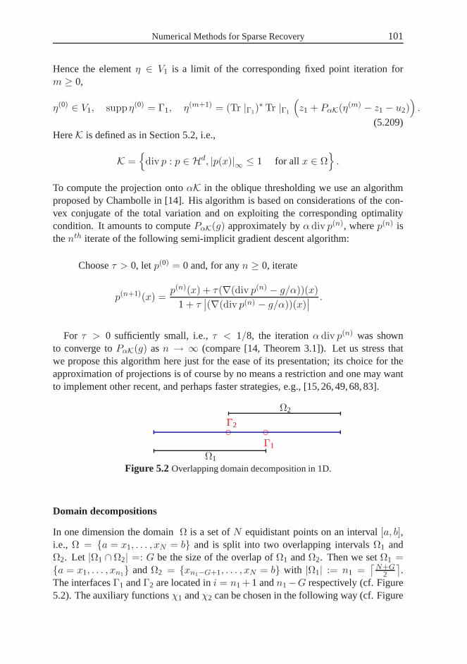
Numerical Methods for Sparse Recovery 101
Hence the elementη ∈ V1 is a limit of the corresponding fixed point iteration form ≥ 0,
η(0) ∈ V1, suppη(0) = Γ1, η(m+1) = (Tr |Γ1)∗ Tr |Γ1
(z1 + PαK(η(m) − z1 − u2)
).
(5.209)HereK is defined as in Section 5.2, i.e.,
K =
div p : p ∈ Hd, |p(x)|∞ ≤ 1 for all x ∈ Ω.
To compute the projection ontoαK in the oblique thresholding we use an algorithmproposed by Chambolle in [14]. His algorithm is based on considerations of the con-vex conjugate of the total variation and on exploiting the corresponding optimalitycondition. It amounts to computePαK(g) approximately byα div p(n), wherep(n) isthenth iterate of the following semi-implicit gradient descent algorithm:
Chooseτ > 0, letp(0) = 0 and, for anyn ≥ 0, iterate
p(n+1)(x) =p(n)(x) + τ(∇(div p(n) − g/α))(x)
1 + τ∣∣(∇(div p(n) − g/α))(x)
∣∣ .
For τ > 0 sufficiently small, i.e.,τ < 1/8, the iterationα div p(n) was shownto converge toPαK(g) asn → ∞ (compare [14, Theorem 3.1]). Let us stress thatwe propose this algorithm here just for the ease of its presentation; its choice for theapproximation of projections is of course by no means a restriction and one may wantto implement other recent, and perhaps faster strategies, e.g., [15,26,49,68,83].
Ω2
Γ2d d
Γ1
Ω1
Figure 5.2Overlapping domain decomposition in 1D.
Domain decompositions
In one dimension the domainΩ is a set ofN equidistant points on an interval[a, b],i.e., Ω = a = x1, . . . , xN = b and is split into two overlapping intervalsΩ1 andΩ2. Let |Ω1 ∩ Ω2| =: G be the size of the overlap ofΩ1 andΩ2. Then we setΩ1 =a = x1, . . . , xn1 andΩ2 = xn1−G+1, . . . , xN = b with |Ω1| := n1 =
⌈N+G
2
⌉.
The interfacesΓ1 andΓ2 are located ini = n1 + 1 andn1−G respectively (cf. Figure5.2). The auxiliary functionsχ1 andχ2 can be chosen in the following way (cf. Figure
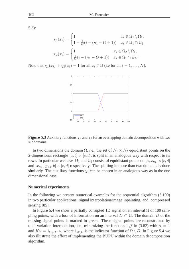
102 M. Fornasier
5.3):
χ1(xi) =
1 xi ∈ Ω1 \ Ω2,
1− 1G(i− (n1 −G+ 1)) xi ∈ Ω1 ∩ Ω2,
χ2(xi) =
1 xi ∈ Ω2 \ Ω1,1G(i− (n1 −G+ 1)) xi ∈ Ω1 ∩ Ω2,
.
Note thatχ1(xi) + χ2(xi) = 1 for all xi ∈ Ω (i.e for all i = 1, . . . ,N ).
10 20 30 40 50 60 70 80 90 100−0.5
0
0.5
1
1.5
2
chi1chi2
Figure 5.3Auxiliary functionsχ1 andχ2 for an overlapping domain decomposition with twosubdomains.
In two dimensions the domainΩ, i.e., the set ofN1 ×N2 equidistant points on the2-dimensional rectangle[a, b] × [c, d], is split in an analogous way with respect to itsrows. In particular we haveΩ1 andΩ2 consist of equidistant points on[a, xn1]× [c, d]and[xn1−G+1, b] × [c, d] respectively. The splitting in more than two domains is donesimilarly. The auxiliary functionsχi can be chosen in an analogous way as in the onedimensional case.
Numerical experiments
In the following we present numerical examples for the sequential algorithm (5.190)in two particular applications: signal interpolation/image inpainting, and compressedsensing [85].
In Figure 5.4 we show a partially corrupted 1D signal on an intervalΩ of 100 sam-pling points, with a loss of information on an intervalD ⊂ Ω. The domainD of themissing signal points is marked in green. These signal points are reconstructed bytotal variation interpolation, i.e., minimizing the functional J in (3.82) withα = 1andKu = 1Ω\D · u, where 1Ω\D is the indicator function ofΩ \D. In Figure 5.4 wealso illustrate the effect of implementing the BUPU within the domain decompositionalgorithm.
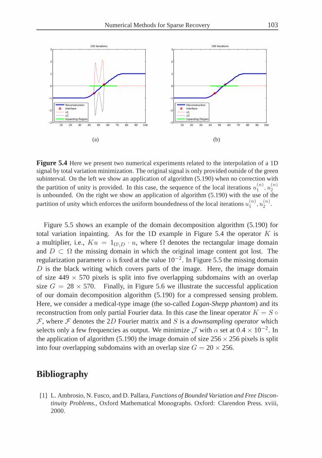
Numerical Methods for Sparse Recovery 103
10 20 30 40 50 60 70 80 90 100−3
−2
−1
0
1
2
3100 iterations
ReconstructionInterfaceu1u2Inpainting Region
(a)
10 20 30 40 50 60 70 80 90 100−3
−2
−1
0
1
2
3100 iterations
ReconstructionInterfaceu1u2Inpainting Region
(b)
Figure 5.4 Here we present two numerical experiments related to the interpolation of a 1Dsignal by total variation minimization. The original signal is only provided outside of the greensubinterval. On the left we show an application of algorithm(5.190) when no correction withthe partition of unity is provided. In this case, the sequence of the local iterationsu(n)
1 , u(n)2
is unbounded. On the right we show an application of algorithm (5.190) with the use of thepartition of unity which enforces the uniform boundedness of the local iterationsu(n)
1 , u(n)2 .
Figure 5.5 shows an example of the domain decomposition algorithm (5.190) fortotal variation inpainting. As for the 1D example in Figure 5.4 the operatorK isa multiplier, i.e.,Ku = 1Ω\D · u, whereΩ denotes the rectangular image domainandD ⊂ Ω the missing domain in which the original image content got lost. Theregularization parameterα is fixed at the value 10−2. In Figure 5.5 the missing domainD is the black writing which covers parts of the image. Here, the image domainof size 449× 570 pixels is split into five overlapping subdomains with an overlapsizeG = 28× 570. Finally, in Figure 5.6 we illustrate the successful applicationof our domain decomposition algorithm (5.190) for a compressed sensing problem.Here, we consider a medical-type image (the so-calledLogan-Shepp phantom) and itsreconstruction from only partial Fourier data. In this casethe linear operatorK = S F , whereF denotes the 2D Fourier matrix andS is adownsampling operatorwhichselects only a few frequencies as output. We minimizeJ with α set at 0.4× 10⁻². Inthe application of algorithm (5.190) the image domain of size 256× 256 pixels is splitinto four overlapping subdomains with an overlap sizeG = 20× 256.
Bibliography
[1] L. Ambrosio, N. Fusco, and D. Pallara,Functions of Bounded Variation and Free Discon-tinuity Problems., Oxford Mathematical Monographs. Oxford: Clarendon Press. xviii,2000.
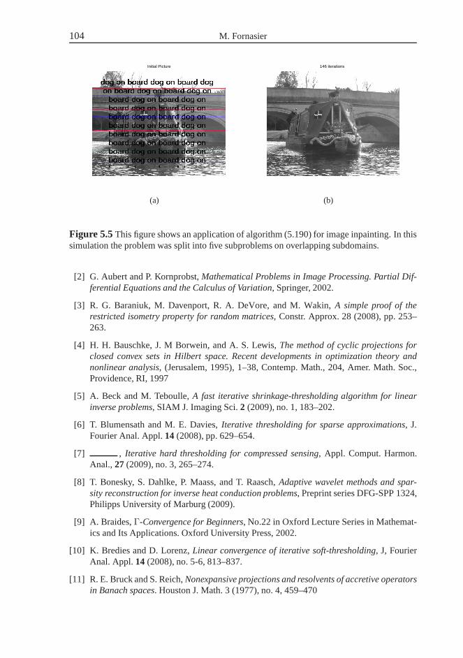
104 M. Fornasier
Initial Picture
(a)
146 iterations
(b)
Figure 5.5This figure shows an application of algorithm (5.190) for image inpainting. In thissimulation the problem was split into five subproblems on overlapping subdomains.
[2] G. Aubert and P. Kornprobst,Mathematical Problems in Image Processing. Partial Dif-ferential Equations and the Calculus of Variation, Springer, 2002.
[3] R. G. Baraniuk, M. Davenport, R. A. DeVore, and M. Wakin,A simple proof of therestricted isometry property for random matrices, Constr. Approx. 28 (2008), pp. 253–263.
[4] H. H. Bauschke, J. M Borwein, and A. S. Lewis,The method of cyclic projections forclosed convex sets in Hilbert space. Recent developments inoptimization theory andnonlinear analysis, (Jerusalem, 1995), 1–38, Contemp. Math., 204, Amer. Math.Soc.,Providence, RI, 1997
[5] A. Beck and M. Teboulle,A fast iterative shrinkage-thresholding algorithm for linearinverse problems, SIAM J. Imaging Sci.2 (2009), no. 1, 183–202.
[6] T. Blumensath and M. E. Davies,Iterative thresholding for sparse approximations, J.Fourier Anal. Appl.14 (2008), pp. 629–654.
[7] , Iterative hard thresholding for compressed sensing, Appl. Comput. Harmon.Anal.,27 (2009), no. 3, 265–274.
[8] T. Bonesky, S. Dahlke, P. Maass, and T. Raasch,Adaptive wavelet methods and spar-sity reconstruction for inverse heat conduction problems, Preprint series DFG-SPP 1324,Philipps University of Marburg (2009).
[9] A. Braides,Γ-Convergence for Beginners, No.22 in Oxford Lecture Series in Mathemat-ics and Its Applications. Oxford University Press, 2002.
[10] K. Bredies and D. Lorenz,Linear convergence of iterative soft-thresholding, J, FourierAnal. Appl.14 (2008), no. 5-6, 813–837.
[11] R. E. Bruck and S. Reich,Nonexpansive projections and resolvents of accretive operatorsin Banach spaces. Houston J. Math. 3 (1977), no. 4, 459–470
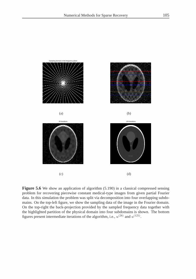
Numerical Methods for Sparse Recovery 105
Sampling domain in the frequency plane
(a) (b)
26 iterations
(c)
126 iterations
(d)
Figure 5.6 We show an application of algorithm (5.190) in a classical compressed sensingproblem for recovering piecewise constant medical-type images from given partial Fourierdata. In this simulation the problem was split via decomposition into four overlapping subdo-mains. On the top-left figure, we show the sampling data of theimage in the Fourier domain.On the top-right the back-projection provided by the sampled frequency data together withthe highlighted partition of the physical domain into four subdomains is shown. The bottomfigures present intermediate iterations of the algorithm, i.e.,u(26) andu(125).
106 M. Fornasier
[12] E. J. Candes, J. Romberg, and T. Tao,Stable signal recovery from incomplete and inac-curate measurements, Comm. Pure Appl. Math. 59 (2006), pp. 1207–1223.
[13] C. Carstensen,Domain decomposition for a non-smooth convex minimalization problemand its application to plasticity, Numerical Linear Algebra with Applications,4 (1998),no. 3, 177–190.
[14] A. Chambolle,An algorithm for total variation minimization and applications. J. Math.Imaging Vision20 (2004), no. 1-2, 89–97.
[15] A. Chambolle, J. Darbon,On total variation minimization and surface evolution usingparametric maximum flows, International Journal of Computer Vision,84 (2009), no. 3,288–307.
[16] A. Chambolle and P.-L. Lions,Image recovery via total variation minimization and re-lated problems., Numer. Math.76 (1997), 167–188.
[17] T. F. Chan, G. H. Golub, and P. Mulet,A nonlinear primal-dual method for totalvariation-based image restoration, SIAM J. Sci. Comput.20 (1999), no. 6, 1964–1977.
[18] T. F. Chan, and T. P. Mathew, Domain decomposition algorithms, Acta Numerica3(1994), pp. 61–143.
[19] A. K. Cline, Rate of convergence of Lawson’s algorithm, Math. Comp.26 (1972), 167–176.
[20] A. Cohen, W. Dahmen, and R. A. DeVore,Compressed sensing and best k-term approx-imation, J. Amer. Math. Soc.22 (2009), 211–231.
[21] P. L. Combettes and V. R. Wajs,Signal recovery by proximal forward-backward splitting,Multiscale Model. Simul.4 (2005), 1168–1200.
[22] S. Dahlke, M. Fornasier, and T. Raasch,Multilevel preconditioning for adaptive sparseoptimization, Preprint 25, DFG-SPP 1324 Preprint Series, 2009
[23] W. Dahmen,Wavelet and multiscale methods for operator equations, Acta Numerica6(1997), 55–228.
[24] W. Dahmen and A. Kunoth,Multilevel preconditioning, Numer. Math63 (1992), 315–344.
[25] G. Dal Maso,An Introduction toΓ-Convergence., Birkhauser, Boston, 1993.
[26] J. Darbon, and M. Sigelle,A fast and exact algorithm for total variation minimization,In LNCS Springer series, 2nd Iberian Conference on Pattern Recognition and ImageAnalysis (IbPria) (2005), 3522(1), 351–359.
[27] I. Daubechies,Ten Lectures on Wavelets, SIAM, 1992.
[28] I. Daubechies, M. Defrise, and C. De Mol,An iterative thresholding algorithm for lin-ear inverse problems with a sparsity constraint, Comm. Pure Appl. Math. 57 (2004),pp. 1413–1457.
[29] I. Daubechies, M. Fornasier, and I. Loris,Accelerated projected gradient methods forlinear inverse problems with sparsity constraints, J. Fourier Anal. Appl.14(2008), no. 5-6, 764–792.
Numerical Methods for Sparse Recovery 107
[30] I. Daubechies, R. A. DeVore, M. Fornasier, and C. S. Gunturk, Iteratively re-weightedleast squares minimization for sparse recovery, Comm. Pure Appl. Math.63 (2010), no.1, 1–38.
[31] R. A. DeVore,Nonlinear approximation, Acta Numerica7 (1998), 51–150.
[32] D. Dobson and C. R. Vogel,Convergence of an iterative method for total variation de-noising, SIAM J. Numer. Anal.34 (1997), no. 5, 1779–1791.
[33] D. L. Donoho,Compressed sensing, IEEE Trans. Inform. Theory52 (2006), 1289–1306.
[34] D. L. Donoho and Y. Tsaig,Fast solution of l1-norm minimization problems when thesolution may be sparse, IEEE Trans. Inform. Theory54 (2008), 4789–4812.
[35] B. Efron, T. Hastie, I. Johnstone, and R. Tibshirani,Least angle regression, Ann. Statist.32 (2004), 407–499.
[36] I. Ekeland and R. Temam,Convex analysis and variational problems, SIAM, 1999.
[37] H. W. Engl, M. Hanke, and A. Neubauer,Regularization of Inverse Problems, Springer-Verlag, 1996.
[38] L. C. Evans and R. F. Gariepy,Measure Theory and Fine Properties of Functions, CRCPress, 1992.
[39] M. Figueiredo and R. D. Nowak,An EM algorithm for wavelet-based image restoration.,IEEE Trans. Image Proc.12 (2003), 906–916.
[40] M. Figueiredo, R. Nowak, and S. J. Wright,Gradient projection for sparse reconstruc-tion: Application to compressed sensing and other inverse problems, IEEE J. SelectedTopics in Signal Process.4 (2007), no. 1, 586–597.
[41] , Sparse reconstruction by separable approximation, IEEE Trans. Signal Proc.57(2009), no. 7, 2479–2493.
[42] M. Fornasier,Domain decomposition methods for linear inverse problems with sparsityconstraints, Inverse Problems23 (2007), 2505–2526.
[43] M. Fornasier, A. Langer and C.-B. Schonlieb,A convergent overlapping domain decom-position method for total variation minimization, preprint 2009.
[44] M. Fornasier and R. March,Restoration of color images by vector valued BV functionsand variational calculus, SIAM J. Appl. Math68 (2007), 437–460.
[45] M. Fornasier and C.-B. Schonlieb,Subspace correction methods for total variation andℓ1-minimization, SIAM J. Numer. Anal.,47 (2009), no. 5, 3397–3428.
[46] A. Y. Garnaev and E. D. Gluskin,On widths of the Euclidean ball, Sov. Math., Dokl.30(1984), 200–204.
[47] E. D. Gluskin,Norms of random matrices and widths of finite-dimensional sets, Math.USSR-Sb.48 (1984), 173–182.
[48] I. F. Gorodnitsky and B. D. Rao,Sparse signal reconstruction from limited data usingFOCUSS: a recursive weighted norm minimization algorithm, IEEE Transactions on Sig-nal Processing45 (1997), 600–616.
108 M. Fornasier
[49] T. Goldstein, S. Osher,The split Bregman method forL1 regularized problems, SIAMJournal on Imaging Sciences,2 (2009), no. 2, 323–343.
[50] J.-B. Hiriart-Urruty and C. Lemarechal,Convex Analysis and Minimization Algorithms I,Vol. 305 of Grundlehren der mathematischen Wissenschaften, Springer-Verlag: Berlin,1996
[51] B. S. Kashin,Diameters of some finite-dimensional sets and classes of smooth functions.,Math. USSR, Izv.11 (1977), 317–333.
[52] S.-J. Kim, K. Koh, M. Lustig, S. Boyd, and D. Gorinevsky,A method for large-scaleℓ1-regularized least squares problems with applications in signal processing and statistics,IEEE Journal Sel. Top. Signal Process.,1 (2007), 606–617.
[53] C. L. Lawson,Contributions to the Theory of Linear Least Maximum Approximation,1961, Ph.D. thesis, University of California, Los Angeles.
[54] G. G. Lorentz, M. v. Golitschek, and Y. Makovoz.Constructive Approximation: Ad-vanced Problems. Springer, Berlin, 1996.
[55] I. Loris, G. Nolet, I. Daubechies, and F. A. Dahlen,Tomographic inversion usingℓ1-normregularization of wavelet coefficients, Geophysical Journal International170 (2007),no. 1, 359–370.
[56] I. Loris, On the performance of algorithms for the minimization of1-penalized function-als, Inverse Problems25 (2009), 035008.
[57] M. Lustig, D. Donoho, and J. M. Pauly,Sparse MRI: The application of compressedsensing for rapid MR imaging, Magnetic Resonance in Medicine58 (2007), no. 6, 1182–1195.
[58] S. Mallat,A Wavelet Tour of Signal Processing: The Sparse Way, Academic Press, 2009.
[59] S. G. Mallat and Z. Zhang,Matching pursuits with time-frequency dictionaries., IEEETrans. Signal Process. 41 (1993), pp. 3397–3415.
[60] J. Muller,Parallel Methods for Nonlinear Imaging Techniques, Master thesis, Universityof Munster, 2008.
[61] B. K. Natarajan,Sparse approximate solutions to linear systems., SIAM J. Comput. 24(1995), pp. 227–234.
[62] Y. Nesterov,Smooth minimization of non-smooth functions. Mathematic Programming,Ser. A,103(2005), 127–152.
[63] Y. Nesterov and A. Nemirovskii,Interior-point polynomial algorithms in convex pro-gramming, SIAM Studies in Applied Mathematics, vol. 13, Society for Industrial andApplied Mathematics (SIAM), Philadelphia, PA, 1994.
[64] Z. Opial,Weak convergence of the sequence of successive approximations for nonexpan-sive mappings, Bull. Amer. Math. Soc.73 (1967), 591–597.
[65] M. Osborne, B. Presnell, and B. Turlach,A new approach to variable selection in leastsquares problems, IMA J. Numer. Anal. 20 (2000), pp. 389–403.
Numerical Methods for Sparse Recovery 109
[66] M. R. Osborne,Finite algorithms in optimization and data analysis, Wiley Series inProbability and Mathematical Statistics: Applied Probability and Statistics, John Wiley& Sons Ltd., Chichester, 1985.
[67] M. Osborne, B. Presnell, and B. Turlach,On the LASSO and its dual, J. Comput. Graph.Statist.9 (2000), 319–337.
[68] S. Osher, M. Burger, D. Goldfarb, J. Xu, and W. Yin,An iterative regularization methodfor total variation-based image restoration, Multiscale Model. Simul.4, no. 2 (2005)460-489.
[69] R. Ramlau, G. Teschke, and M. Zhariy,A compressive Landweber iteration for solvingill-posed inverse problems, Inverse Problems24 (2008), no. 6, 065013.
[70] H. Rauhut,Compressive Sensing and Structured Random Matrices. In Theoretical Foun-dations and Numerical Methods for Sparse Recovery, Radon Series Comp. Appl. Math.deGruyter, 2010.
[71] R.T. Rockafellar and R. J. B. Wets,Variational analysis, Grundlehren der Mathematis-chen Wissenschaften, vol. 317, Springer-Verlag, Berlin, 1998.
[72] L. Rudin, S. Osher, and E. Fatemi,Nonlinear total variation based noise removal algo-rithms., Physica D60 (1992), 259–268.
[73] C.-B. Schonlieb,Total variation minimization with anH−1 constraint, CRM Series 9,Singularities in Nonlinear Evolution Phenomena and Applications proceedings, ScuolaNormale Superiore Pisa 2009, 201–232.
[74] J.-L. Starck, E. J. Candes, and D. L. Donoho,Astronomical image representation bycurvelet transform, Astronomy and Astrophysics298(2003), 785–800.
[75] J.-L. Starck, M. K. Nguyen, and F. Murtagh,Wavelets and curvelets for image deconvo-lution: a combined approach, Signal Proc.83 (2003), 2279–2283.
[76] R. Tibshirani,Regression shrinkage and selection via the lasso, J. Roy. Statist. Soc. Ser.B 58 (1996), 267–288.
[77] J. A. Tropp and D. Needell,CoSaMP: Iterative signal recovery from incomplete andinaccurate samples, Appl. Comput. Harmon. Anal.26 (2008), no. 3, 301–321.
[78] J. A. Tropp,Greed is good: Algorithmic results for sparse approximation, IEEE Trans.Inform. Theory50 (2004), 2231–2242.
[79] X.-C. Tai and P. Tseng,Convergence rate analysis of an asynchronous space decomposi-tion method for convex minimization, Math. Comp.71 (2001), no. 239, 1105–1135.
[80] X.-C. Tai and J. Xu,Global convergence of subspace correction methods for convexoptimization problems, Math. Comp.,71 (2002), no. 237, 105–124.
[81] L. Vese,A study in the BV space of a denoising-deblurring variational problem., Appl.Math. Optim.44 (2001), 131–161.
[82] J. Warga,Minimizing certain convex functions, J. Soc. Indust. Appl. Math.11 (1963),588–593.
110 M. Fornasier
[83] P. Weiss, L. Blanc-Feraud, and G. Aubert,Efficient schemes for total variation mini-mization under constraints in image processing, SIAM J. Sci. Comput.,31 (2009, no. 3,2047–2080.
[84] J. Xu, X.-C. Tai and L.-L. Wang,A two-level domain decomposition method for imagerestoration, UCLA Computational and Applied Mathematics Report 09-92,November2009.
[85] Matlab code and numerical experiments for the domain decompositionmethods presented in this chapter can be downloaded at the web-page:http://homepage.univie.ac.at/carola.schoenlieb/webpage$\_$tvdode/tv$\_$dode$\_$numerics.htm
Author information
Massimo Fornasier, RICAM, Austrian Academy of Sciences, Linz, Austria.E-mail:[email protected]