numerical methods for hyperbolic system of conservation...
TRANSCRIPT
Numerical methods for hyperbolic system of
conservation laws
Praveen ChandrashekarCentre for Applicable Mathematics
Tata Institute of Fundamental ResearchBangalore-560065
http://cpraveen.github.io
August 13, 2019

Contents
1 Conservation law 41.1 Notion of weak solution . . . . . . . . . . . . . . . . . . . . . . . . . . . . . . . . . . . 51.2 Jump conditions . . . . . . . . . . . . . . . . . . . . . . . . . . . . . . . . . . . . . . . 51.3 Entropy condition . . . . . . . . . . . . . . . . . . . . . . . . . . . . . . . . . . . . . . 51.4 Euler equations . . . . . . . . . . . . . . . . . . . . . . . . . . . . . . . . . . . . . . . . 6
1.4.1 Non-conservative form . . . . . . . . . . . . . . . . . . . . . . . . . . . . . . . . 81.4.2 Entropy equation . . . . . . . . . . . . . . . . . . . . . . . . . . . . . . . . . . . 8
1.5 Isothermal/isentropic gas . . . . . . . . . . . . . . . . . . . . . . . . . . . . . . . . . . 91.6 p-system . . . . . . . . . . . . . . . . . . . . . . . . . . . . . . . . . . . . . . . . . . . . 91.7 Linearized Euler equations . . . . . . . . . . . . . . . . . . . . . . . . . . . . . . . . . . 101.8 Shallow water equations . . . . . . . . . . . . . . . . . . . . . . . . . . . . . . . . . . . 101.9 Maxwell’s equations . . . . . . . . . . . . . . . . . . . . . . . . . . . . . . . . . . . . . 10
2 FVM in 1-D 112.1 Basic scheme . . . . . . . . . . . . . . . . . . . . . . . . . . . . . . . . . . . . . . . . . 112.2 Local truncation error . . . . . . . . . . . . . . . . . . . . . . . . . . . . . . . . . . . . 122.3 Implementation of scheme . . . . . . . . . . . . . . . . . . . . . . . . . . . . . . . . . . 13
3 Linear hyperbolic system in 1-D 153.1 Where are the waves ? . . . . . . . . . . . . . . . . . . . . . . . . . . . . . . . . . . . . 153.2 General solution . . . . . . . . . . . . . . . . . . . . . . . . . . . . . . . . . . . . . . . 163.3 Riemann problem . . . . . . . . . . . . . . . . . . . . . . . . . . . . . . . . . . . . . . . 163.4 Upwind scheme . . . . . . . . . . . . . . . . . . . . . . . . . . . . . . . . . . . . . . . . 19
4 Euler equations in 1-D 214.1 Flux Jacobian . . . . . . . . . . . . . . . . . . . . . . . . . . . . . . . . . . . . . . . . . 214.2 Hyperbolicity . . . . . . . . . . . . . . . . . . . . . . . . . . . . . . . . . . . . . . . . . 224.3 Homogeneity property . . . . . . . . . . . . . . . . . . . . . . . . . . . . . . . . . . . . 224.4 Primitive form . . . . . . . . . . . . . . . . . . . . . . . . . . . . . . . . . . . . . . . . 234.5 Entropy equation . . . . . . . . . . . . . . . . . . . . . . . . . . . . . . . . . . . . . . . 244.6 Characteristic form . . . . . . . . . . . . . . . . . . . . . . . . . . . . . . . . . . . . . . 254.7 Jump conditions . . . . . . . . . . . . . . . . . . . . . . . . . . . . . . . . . . . . . . . 25
4.7.1 Contact/shear wave . . . . . . . . . . . . . . . . . . . . . . . . . . . . . . . . . 264.7.2 Shock wave . . . . . . . . . . . . . . . . . . . . . . . . . . . . . . . . . . . . . . 26
4.8 Riemann problem (Shock tube problem) . . . . . . . . . . . . . . . . . . . . . . . . . . 27
5 Lax-Friedrich flux 325.1 Rusanov or local Lax-Friedrich scheme . . . . . . . . . . . . . . . . . . . . . . . . . . . 325.2 Positivity property . . . . . . . . . . . . . . . . . . . . . . . . . . . . . . . . . . . . . . 33
6 Flux Vector Splitting schemes 346.1 Steger-Warming scheme . . . . . . . . . . . . . . . . . . . . . . . . . . . . . . . . . . . 346.2 van Leer splitting . . . . . . . . . . . . . . . . . . . . . . . . . . . . . . . . . . . . . . . 35
6.2.1 van Leer: Mass flux . . . . . . . . . . . . . . . . . . . . . . . . . . . . . . . . . 36
1

CONTENTS 2
6.2.2 van Leer: momentum flux . . . . . . . . . . . . . . . . . . . . . . . . . . . . . . 366.2.3 van Leer: Energy flux . . . . . . . . . . . . . . . . . . . . . . . . . . . . . . . . 366.2.4 van Leer flux . . . . . . . . . . . . . . . . . . . . . . . . . . . . . . . . . . . . . 36
6.3 Liou and Steffen (1993) . . . . . . . . . . . . . . . . . . . . . . . . . . . . . . . . . . . 376.4 Zha-Bilgen flux vector splitting (1993) . . . . . . . . . . . . . . . . . . . . . . . . . . . 37
7 Godunov scheme 40
8 Roe scheme 428.1 Roe scheme: entropy violation . . . . . . . . . . . . . . . . . . . . . . . . . . . . . . . . 448.2 Roe scheme formulae . . . . . . . . . . . . . . . . . . . . . . . . . . . . . . . . . . . . . 448.3 Roe scheme for general system . . . . . . . . . . . . . . . . . . . . . . . . . . . . . . . 45
9 HLL and HLLC Riemann solvers 479.1 HLL Riemann solver . . . . . . . . . . . . . . . . . . . . . . . . . . . . . . . . . . . . . 47
9.1.1 Estimation of wave speeds, entropy condition . . . . . . . . . . . . . . . . . . . 489.1.2 Positivity of intermediate state . . . . . . . . . . . . . . . . . . . . . . . . . . . 49
9.2 HLLC Riemann solver . . . . . . . . . . . . . . . . . . . . . . . . . . . . . . . . . . . . 49
10 FVM in 1-D: high order schemes 5110.0.1 Second order SSPRK . . . . . . . . . . . . . . . . . . . . . . . . . . . . . . . . . 5110.0.2 Third order SSPRK . . . . . . . . . . . . . . . . . . . . . . . . . . . . . . . . . 51
10.1 Estimate of reconstruction slope . . . . . . . . . . . . . . . . . . . . . . . . . . . . . . 5210.2 Local truncation error . . . . . . . . . . . . . . . . . . . . . . . . . . . . . . . . . . . . 52
11 2-D finite volume method 5311.1 First order scheme . . . . . . . . . . . . . . . . . . . . . . . . . . . . . . . . . . . . . . 5311.2 Implementation of scheme . . . . . . . . . . . . . . . . . . . . . . . . . . . . . . . . . . 5411.3 Second order scheme . . . . . . . . . . . . . . . . . . . . . . . . . . . . . . . . . . . . . 5411.4 Higher order scheme . . . . . . . . . . . . . . . . . . . . . . . . . . . . . . . . . . . . . 55
11.4.1 Solution reconstruction . . . . . . . . . . . . . . . . . . . . . . . . . . . . . . . 5611.4.2 Flux quadrature . . . . . . . . . . . . . . . . . . . . . . . . . . . . . . . . . . . 56
12 ENO and WENO schemes 5712.1 1-D grid . . . . . . . . . . . . . . . . . . . . . . . . . . . . . . . . . . . . . . . . . . . . 5712.2 First order finite volume scheme . . . . . . . . . . . . . . . . . . . . . . . . . . . . . . 5712.3 Higher order finite volume scheme . . . . . . . . . . . . . . . . . . . . . . . . . . . . . 5712.4 ENO scheme . . . . . . . . . . . . . . . . . . . . . . . . . . . . . . . . . . . . . . . . . 58
12.4.1 Polynomial reconstruction . . . . . . . . . . . . . . . . . . . . . . . . . . . . . . 5812.4.2 Primitive function . . . . . . . . . . . . . . . . . . . . . . . . . . . . . . . . . . 5912.4.3 Construction of Pj(x) . . . . . . . . . . . . . . . . . . . . . . . . . . . . . . . . 5912.4.4 Newton form of reconstruction . . . . . . . . . . . . . . . . . . . . . . . . . . . 5912.4.5 Smoothness indicator . . . . . . . . . . . . . . . . . . . . . . . . . . . . . . . . 60
12.5 ENO reconstruction . . . . . . . . . . . . . . . . . . . . . . . . . . . . . . . . . . . . . 6012.6 TVB property of ENO reconstruction . . . . . . . . . . . . . . . . . . . . . . . . . . . 6112.7 Sign property of ENO scheme . . . . . . . . . . . . . . . . . . . . . . . . . . . . . . . . 6212.8 WENO scheme . . . . . . . . . . . . . . . . . . . . . . . . . . . . . . . . . . . . . . . . 62
12.8.1 Third order approximation for vLi+ 1
2
: k = 2 . . . . . . . . . . . . . . . . . . . . 62
12.8.2 Fifth order approximation for vLi+ 1
2
: k = 3 . . . . . . . . . . . . . . . . . . . . . 63
12.8.3 Non-linear blending . . . . . . . . . . . . . . . . . . . . . . . . . . . . . . . . . 6412.8.4 WENO-JS scheme . . . . . . . . . . . . . . . . . . . . . . . . . . . . . . . . . . 6412.8.5 Characteristic variable reconstruction . . . . . . . . . . . . . . . . . . . . . . . 66
12.9 Example: error convergence . . . . . . . . . . . . . . . . . . . . . . . . . . . . . . . . . 6612.10Example: Periodic advection of isentropic vortex . . . . . . . . . . . . . . . . . . . . . 67

CONTENTS 3
12.11Finite volume WENO in 2-D . . . . . . . . . . . . . . . . . . . . . . . . . . . . . . . . 6812.12Finite difference WENO scheme . . . . . . . . . . . . . . . . . . . . . . . . . . . . . . . 68
12.12.1 Analysis of WENO-JS scheme . . . . . . . . . . . . . . . . . . . . . . . . . . . . 6912.12.2 WENO-Z scheme . . . . . . . . . . . . . . . . . . . . . . . . . . . . . . . . . . . 70
12.13Central WENO (CWENO) schemes . . . . . . . . . . . . . . . . . . . . . . . . . . . . 70
A Euler test cases 71A.1 1-D: linear advection . . . . . . . . . . . . . . . . . . . . . . . . . . . . . . . . . . . . . 71A.2 1-D: Sod test . . . . . . . . . . . . . . . . . . . . . . . . . . . . . . . . . . . . . . . . . 71A.3 1-D: Sod test with sonic rarefaction . . . . . . . . . . . . . . . . . . . . . . . . . . . . . 71A.4 1-D: Shu-Osher test case . . . . . . . . . . . . . . . . . . . . . . . . . . . . . . . . . . . 71A.5 1-D: 123 problem . . . . . . . . . . . . . . . . . . . . . . . . . . . . . . . . . . . . . . . 72A.6 1-D: Interaction of blast waves . . . . . . . . . . . . . . . . . . . . . . . . . . . . . . . 72A.7 2-D: Isentropic vortex . . . . . . . . . . . . . . . . . . . . . . . . . . . . . . . . . . . . 72A.8 2-D: Shock reflection . . . . . . . . . . . . . . . . . . . . . . . . . . . . . . . . . . . . . 73

Chapter 1
Conservation law
Let us consider a system of coupled equations of the form
∂U
∂t+
d∑j=1
∂
∂xjFj(U) = 0 (1.1)
where U is called the set of conserved variables and Fj are the flux vectors
U =
U1
U2
.
.Up
∈ Uad ⊂ Rp, Fj =
F1j
F2j
.
.Fpj
∈ Rp, 1 ≤ j ≤ d
Here Uad is the set of physically admissible states and depends on the particular problem we aredealing with.
For any spatial domain D ⊂ Rd with outward unit normal vector n = (n1, . . . , nd) to ∂D
d
dt
∫DUdx+
d∑j=1
∫∂D
Fj(U)njdS = 0
The above equations tell us that the total amount of U inside any domain D changes only due to thefluxes across the domain boundary. Due to this property, we say that we have a system of conservationlaws.
Define the flux jacobian
Aj(U) = F ′j(U) =
[∂
∂UkFij(U)
]1≤i,k≤p
∈ Rp×p
Definition 1.1 (Hyperbolicity). The system of conservation laws (1.1) is said to be hyperbolic if forevery U ∈ Uad and for every ω = (ω1, . . . , ωd) ∈ Rd, the matrix
A(U, ω) =d∑j=1
Aj(U)ωj
1. has p real eigenvalues λ1(U, ω) ≤ λ2(U, ω) ≤ . . . ≤ λp(U, ω)
2. and p linearly independent eigenvectors r1(U, ω), . . . , rp(U, ω), i.e.,
A(U, ω)rj(U, ω) = λj(U, ω)rj(U, ω) 1 ≤ j ≤ p
Moreover, if the eigenvalues are all distinct, then it is said to be strictly hyperbolic. In this case,condition (2) is automatically satisfied.
4

CHAPTER 1. CONSERVATION LAW 5
Definition 1.2 (Cauchy problem or Initial Value Problem (IVP)). Find a function U : (x, t) ∈Rd × [0,∞)→ U(x, t) ∈ Uad which is a solution of (1.1) and satisfies the initial condition
U(x, 0) = U0(x) x ∈ Rd
Example 1.3 (Riemann problem (1-D)). This corresponds to the IVP with initial condition
U(x, 0) = U0(x) =
Ul x < 0
Ur x > 0
1.1 Notion of weak solution
The solution of hyperbolic PDE can develop discontinuities even when the initial condition and otherdata are very smooth. We would like to allow discontinuous solutions since they are observed in manyphysical phenomena. The classical notion of solution which requires all derivatives appearing in thePDE to exist is not valid in this case. Instead, let us multiply the conservation law by a smooth testfunction with compact support in space and time∫
R+
∫Rd
(∂tU + ∂jFj(U)) · Φdxdt = 0, Φ ∈ C1c (Rd × R+;Rp)
and do integration by parts to transfer derivatives onto the test function∫R+
∫Rd
(U · ∂tΦ + Fj(U) · ∂jΦ)dxdt+
∫Rd
U(x, 0)Φ(x, 0)dx = 0, ∀Φ ∈ C1c (Rd × R+;Rp)
This equation makes sense even if the function U is not smooth, as long as the integrals exist. If aweak solution is smooth, then it is also a classical solution.
1.2 Jump conditions
Consider a discontinuity in the solution across the surface
x = X(t)
The solution on either side of the discontinuity surface cannot be arbitrary but must satisfy theRankine-Hugoniot jump conditions
JFjnjK = S JUK
whereS = Xjnj
is normal speed of the discontinuity surface. This can be proved starting from the definition ofweak solution. Moreover, a piecewise smooth solution which satisfies the jump condition at points ofdiscontinuity is a weak solution.
1.3 Entropy condition
The price we pay for adopting the notion of weak solutions is that we lose uniqueness. There can bemultiple or an infinite number of solutions that satisfy the definition of weak solution. In order toselect a unique solution among the set of all weak solutions, we need an additional principle, whichis usually called an entropy condition. For physical problems, the laws of thermodynamics must holdand the second law says that the entropy of an isolated system cannot decrease with time. This notioncan be introduced for a general system of conservation laws in the following way.
Assume that we have a strictly convex function Q = Q(U) called the entropy function and associ-ated entropy fluxes Gj such that
Q′(U)F ′j(U) = G′j(U), 1 ≤ j ≤ d

CHAPTER 1. CONSERVATION LAW 6
The set of functions (Q(U), Gj(U)) is called an entropy pair. Multiply the conservation law by Q′(U)
Q′(U)∂tU +Q′(U)∂jFj(U) = 0
∂tQ(U) +Q′(U)F ′j(U)∂jU = 0
∂tQ(U) + ∂jGj(U) = 0
Hence smooth solutions of the conservation law satisfy the additional entropy conservation law. How-ever, we cannot expect that the entropy equation holds for discontinuous solutions, since the entropyjump conditions may not be consistent with the jump conditions of conservation law.
Usually, it happens that hyperbolic equation is a simplification of a more realistic model wherecertain terms of small order have been dropped. An important realistic model involves parabolic terms
∂tU + ∂jFj(U) = ε∆U, ε > 0
Because ε 1 in many physical situations, we might have dropped this term from our model. However,we lose some important information, the entropy condition, when we throw away the Laplacian term.Multiplying throughout by Q′(U)
Q′(U)∂tU +Q′(U)F ′j(U)∂jU = εQ′(U)∂2jU
= ε∂j [Q′(U)∂jU ]− ε[∂jU ]>Q′′(U)∂jU︸ ︷︷ ︸
≥0
As Q(U) is strictly convex, the hessian Q′′(U) is symmetric, positive definite, and we obtain theinequality
∂tQ(U) + ∂jGj(U) ≤ ε∂j [Q′(U)∂jU ]
In the limit of ε→ 0, we obtain the entropy inequality
∂tQ(U) + ∂jGj(U) ≤ 0
We will demand that this inequality must be satisfied in the weak sense. Across a discontinuity movingwith speed S,
JGjnjK ≤ S JQK
must be satisfied.
1.4 Euler equations
The Euler equations model the flow of ideal gas in which there is no frictional effects. In such a fluid,the stress field is isotropic and given by a scalar pressure field p. The equations are mathematicalstatements of conservation laws of mass, momentum and energy. We can derive these equations byconsidering a fixed control volume V and writing down the conservation law. Let
ρ mass density, i.e., mass per unit volume, Kg/m3
v = (v1, v2, v3) velocity vector, m/sp pressure, N/m2
The quantities (ρ, v, p) completely specify the state of the system at any particular time.
Mass conservation The mass inside V changes due to flow of fluid across the boundary of V , whichwe denote by ∂V . Net mass flow out of ∂V happens only due to the normal component of velocity.Hence
d
dt
∫Vρdx = −
∮∂Vρ(v · n)ds = −
∫V∇ · (ρv)dx
where we used Gauss divergence theorem. Since this must hold for every control volume, we deducethe condition
∂ρ
∂t+∇ · (ρv) = 0
or in index notation∂tρ+ ∂j(ρvj) = 0
CHAPTER 1. CONSERVATION LAW 7
Momentum equation This is just Newton’s law applied to fluids. Let f be some external forcefield per unit volume, e.g., gravity, electromagnetic force, etc. Then Newton’s law is
d
dt
∫Vρvdx = −
∮∂V
(ρv)(v · n)ds+
∮∂Vpnds+
∫Vρfdx = −
∫V
(ρv ⊗ v + pI)dx+
∫Vρfdx
and hence we obtain the equation
∂
∂t(ρv) +∇ · (ρv ⊗ v + pI) = ρf
or in index notation∂t(ρvi) + ∂j(ρvivj + pδij) = ρfi, i = 1, 2, 3
Remark 1.4. If gravity is acting in the negative x3 direction, then f = (0, 0,−g) where g = 9.81 m2/sis the acceleration due to gravity.
Energy conservation The first law of thermodynamics says that the total energy of an isolatedsystem is conserved. For a system that interacts with its environment, the total energy changes dueto flow of energy into/out of V and the work done on the system. In an ideal fluid, energy flows onlydue to convection by the flow, i.e., we ignore effects like conduction of heat. Let
E = total energy per unit volume, J/m3
Then the energy conservation law is
d
dt
∫VEdx = −
∮∂VE(v · n)dx−
∮∂Vp(v · n)ds+
∫Vρf · vdx
Using divergence theorem, we obtain
∂E
∂t+∇ · (Ev + pv) = ρf · v
or in index notation∂tE + ∂j [(E + p)vj ] = ρfjvj
The total energy is made up of internal energy, kinetic energy, gravitational energy, etc. Let us assumethat only internal and kinetic energy are relevant in our problem. Then
E = ρe+1
2ρ|v|2
where e = e(ρ, p) is the internal energy per unit mass. For a calorically perfect gas
e = cvT, cv = constant
combined with ideal gas lawp = ρRT
yields
cv =R
γ − 1=⇒ e =
p
(γ − 1)ρ
whereγ =
cpcv> 1
is the ratio of specific heats at constant pressure and constant volume, respectively. For air which ismostly composed of nitrogen, γ = 1.4. The total energy is given by
E =p
γ − 1+
1
2ρ|v|2 =⇒ p = (γ − 1)
[E − 1
2ρ|v|2
]

CHAPTER 1. CONSERVATION LAW 8
Summary of equations All of the conservation laws we have derived have a common structure
∂
∂t(some density) +∇ · (corresponding flux) = source term
We can hence write the Euler equations as
∂tU + ∂jFj(U) = S(U)
where
U =
ρρv1
ρv2
ρv3
E
, F1 =
ρv1
p+ ρv21
ρv1v2
ρv1v3
(E + p)v1
, F2 =
ρv2
ρv2v1
p+ ρv22
ρv2v3
(E + p)v2
, F3 =
ρv3
ρv3v1
ρv3v2
p+ ρv23
(E + p)v3
S =
0ρf1
ρf2
ρf3
ρ(f1v1 + f2v2 + f3v3)
, p = (γ − 1)
[E − 1
2ρ|v|2
]
This is a hyperbolic system for which the matrix A(U, ω) has real eigenvalues
v · ω − a, v · ω, v · ω, v · ω, v · ω + a
where
a =
√γp
ρ
is the speed of sound. Though there are repeated eigenvalues, we can find a full set of eigenvectors.
State space Physically admissible states must have strictly positive values of density and pressure,i.e.,
ρ > 0, p > 0 =⇒ Uad =
U ∈ R5 : U1 > 0, U5 −
1
2U1(U2
2 + U23 + U2
4 ) > 0
This is a convex subset of R5. It is very important that the numerical scheme should yield positivesolutions, since otherwise, the computations will break down.
1.4.1 Non-conservative form
It is some times useful to write the Euler equations in non-conservative form. They are given by
∂ρ
∂t+ v · ∇ρ+ ρ∇ · v = 0
∂v
∂t+ v · ∇v +
1
ρ∇p = 0
∂p
∂t+ v · ∇p+ γp∇ · v = 0
1.4.2 Entropy equation
The thermodynamic entropy can be taken as
s =p
ργ
and using the Euler equations, we can derive the entropy equation
∂s
∂t+ v · ∇s = 0
CHAPTER 1. CONSERVATION LAW 9
This implies that entropy of a fluid element is constant. Using the continuity equation we can rewritethis in conservation form
∂
∂t(ρs) +∇ · (ρsv) = 0
In fact a more general equation holds. Define
Q = ρH(s), Gj = ρvjH(s)
Then∂tQ+ ∂jGj = 0
holds for smooth solutions. Moreover, ifH ′(s) < 0 thenQ(U) is a strictly convex function1. For Navier-Stokes equations with Fourier law of heat conduction, the correct entropy function is H(s) = − ln(s)so that
Q = −ρ ln s, Gj = −ρvj ln s
1.5 Isothermal/isentropic gas
If the gas system behaves in such a way that
p = p(ρ)
then the energy equation is not required and we have just mass and momentum equation
∂ρ
∂t+∇ · (ρv) = 0
∂(ρv)
∂t+∇ · (ρv ⊗ v + p(ρ)I) = 0
If the gas temperature is constant, then ideal gas assumption implies that
p = Cρ =⇒ Isothermal Euler equations
If the gas has constant entropy, then
p = Cργ =⇒ Isentropic Euler equations
for some γ > 1. In both cases, we have a hyperbolic system of equations. For these models, the totalenergy E plays the role of a convex entropy function.
1.6 p-system
Model for one-dimensional isentropic gas dynamics in Lagrangian coordinates
∂v
∂t− ∂u
∂x= 0
∂u
∂t+
∂
∂xp(v) = 0
v = specific volume = 1ρ
u = velocityp = pressure = Cv−γ , γ ≥ 1 “Conserved” variables and flux vector
U =
[vu
], F =
[−up(v)
], Uad = (v, u) ∈ R2 : v > 0
Flux jacobian
A = F ′(U) =
[0 −1
p′(v) 0
]Eigenvalues are real and distinct provided p′(v) < 0
λ1 = −√−p′(v), λ2 =
√−p′(v)
1See Bouchut
CHAPTER 1. CONSERVATION LAW 10
1.7 Linearized Euler equations
In some problems, the flow may be constant with only small perturbations around a constant state(ρ0, v0, p0). In this case, the flow may be treated as isentropic
p = p(ρ, s) = C(s)ργ
and we can ignore the energy equation. Then
ρ = ρ0 + ρ′, v = v0 + v′, p = p(ρ0) + p′ = p0 + (γp0/ρ0)ρ′
where|ρ′| ρ0, |v′| |v0|
Ignoring terms quadratic in the perturbations, the mass and momentum equations take the form
∂ρ′
∂t+ v0 · ∇ρ′ + ρ′∇ · v0 = 0
∂v′
∂t+ v0 · ∇v′ + v′ · ∇v0 +
a20
ρ0∇ρ′ = 0, a0 =
√γp0/ρ0
This is a hyperbolic system.We can also take the linearized pressure equation
∂p′
∂t+ v0 · ∇p′ + γp0∇ · v′ = 0
instead of the density equation.
Sound waves Let us consider the background state to be stationary, v0 = 0. Then
∂v′
∂t+
1
ρ0∇p′ = 0,
∂p′
∂t+ γp0∇ · v′ = 0
Differentiating pressure equation wrt time
∂ttp′ + γp0∇ · ∂tv′ = 0 =⇒ ∂ttp
′ = a20∆p′
The pressure perturbations are governed by the wave equations and the perturbations propagate withspeed a0 which is the sound speed.
1.8 Shallow water equations
1.9 Maxwell’s equations

Chapter 2
FVM in 1-D
The finite volume method is based on the integral form of the conservation laws and gives an approx-imation to the weak solution. Consider a 1-D conservation law system
Ut + F (U)x = 0
with some initial conditionU(x, 0) = U0(x)
We partition the domain into disjoint cells
Ij+ 12
= [xj− 12, xj+ 1
2], ∆x = xj+ 1
2− xj− 1
2, xj =
1
2(xj− 1
2+ xj+ 1
2)
Integrate the conservation law over one cell
d
dt
∫Ij+1
2
U(x, t)dx+ F (xj+ 12, t)− F (xj− 1
2, t) = 0
Define the cell average value
Uj(t) =1
∆x
∫Ij+1
2
U(x, t)dx
We have to make some approximation to estimate the fluxes. Suppose we have some method to dothis
F (xj+ 12, t) ≈ Fj+ 1
2(t) = F (. . . , Uj(t), Uj+1(t), . . .)
and Fj+ 12
is called a numerical flux function. We obtain the semi-discrete finite volume scheme
∆xdUjdt
+ Fj+ 12− Fj− 1
2= 0
2.1 Basic scheme
The numerical solution is defined by the cell averages, which give a piecewise constant approximation.Suppose
Fj+ 12
= F (Uj , Uj+1)
where the numerical flux is constant in the sense that
F (U,U) = F (U) ∀U ∈ Uad
We partition the time axis into intervals ∆t; we will compute the numerical solution at the time levels
tn = n∆t, n = 0, 1, 2, . . .
11

CHAPTER 2. FVM IN 1-D 12
and denote the cell average byUnj ≈ U(x, tn) x ∈ Ij+ 1
2
The superscript denotes the time level and is not a power. The time derivative can be approximatedby a forward difference formula in time, also called forward Euler scheme
dUjdt
(tn) ≈Un+1j − Unj
∆t
Then the fully discrete scheme is
∆xUn+1j − Unj
∆t+ Fn
j+ 12
− Fnj− 1
2
= 0
Since the solution is known at time level n, we put all these quantities on the right hand side to obtainthe finite volume update equation
Un+1j = Unj −
∆t
∆x[Fnj+ 1
2
− Fnj− 1
2
], n = 0, 1, 2, . . .
Given the initial condition
U0j = U0(xj) or U0
j =1
∆x
∫Ij+1
2
U0(x)dx
we repeatedly apply the update equation to generate the solution at future times.
Remark 2.1. How to compute the numerical flux ? This is the key question in the finite volumemethod. The natural thing to try is to perform some interpolation, for example
Fj+ 12
=1
2[Fj + Fj+1]
but this leads to a central difference scheme
∆xdUjdt
+1
2(Fj+1 − Fj−1) = 0
which is unstable for non-linear hyperbolic problems. In the remaining chapters, we will see better waysto approximate the flux. The piece-wise constant solution representation creates a Riemann problemat each cell face. We can solve the Riemann problem exactly or approximately to compute the flux.
2.2 Local truncation error
The local truncation error is useful to make some conclusions on the order of accuracy that can beexpected from the scheme. Let us assume that we have a consistent numerical flux function andalso that it is a smooth function of its two arguments. The local truncation error is obtained bysubstituting a smooth exact solution into the numerical scheme
Th =U(x, t+ ∆t)− U(x, t)
∆t+F (U(x, t), U(x+ ∆x, t))− F (U(x−∆x, t), U(x, t))
∆x
We perform Taylor expansion around (x, t). The first term is
U(x, t+ ∆t)− U(x, t)
∆t= ∂tU(x, t) +O (∆t)
Define shorthand notationU = U(x, t), ∂xU = ∂xU(x, t)

CHAPTER 2. FVM IN 1-D 13
Let us call the two arguments of F (·, ·) are X,Y respectively. Then, differentiating the flux consistencycondition, we get
∂
∂XF (U,U) +
∂
∂YF (U,U) =
∂
∂UF (U)
Now
F (U(x, t), U(x+ ∆x, t)) = F (U,U + ∆x∂xU +O(∆x2
))
= F (U,U) + ∆x∂
∂YF (U,U) · ∂xU +O
(∆x2
)= F (U) + ∆x
∂
∂YF (U,U) · ∂xU +O
(∆x2
)and similarly
F (U(x−∆x, t), U(x, t)) = F (U)−∆x∂
∂XF (U,U) · ∂xU +O
(∆x2
)The flux difference term becomes
F (U(x, t), U(x+ ∆x, t))− F (U(x−∆x, t), U(x, t))
∆x
=
[∂
∂XF (U,U) +
∂
∂YF (U,U)
]∂xU +O (∆x)
=∂
∂UF (U) · ∂xU +O (∆x)
= ∂xF +O (∆x)
Hence the truncation error is
Th = ∂tU + ∂xF +O (∆t) +O (∆x) = O (∆t) +O (∆x)
We get first order accuracy just from a smooth, consistent flux.
2.3 Implementation of scheme
Let us write the scheme in residual form
∆xdUjdt
+Rj = 0, Rj = Fj+ 12− Fj− 1
2
The update equation is
Un+1j = Unj −
∆t
∆xRnj
Note that the flux Fj+ 12
appears in Rj as shown above and also in Rj+1
Rj+1 = Fj+ 32− Fj+ 1
2
but with opposite sign. Since the flux computation can be expensive, we will compute each flux onlyonce and add/subtract it from the two residuals. This requires that we should loop over the faces.The algorithm is given in (1). To implement this method, we need arrays to store the solution andthe residual. Here is a Fortran-type pseudo-code. It uses Neumann boundary conditions at both endsof the domain.

CHAPTER 2. FVM IN 1-D 14
Algorithm 1: First order finite volume scheme
Allocate memory for all variables;Set initial condition;Set time counter t = 0;while t < T do
Compute time step ∆t;Set residual to zero;for each face do
Compute flux;Add flux to left residual;Subtract flux from right residual;
endUpdate solution to next time level;t = t+ ∆t;
end
Listing 2.1: First order FVM
integer : : nvar=3, nx=100 , j
real : : U (nvar , nx ) , R (nvar , nx ) , flux ( nvar ) , t , dt , T=1.0 , &cfl=0.9
call set_initial_condition (U ) ! Set i n i t i a l cond i t i on in Ut = 0.0do while (t < T )
dt = compute_dt (cfl , U ) ! Compute time step us ing CFL cond i t i onR = 0do j=0,nx
if (j == 0) then ! f i r s t f a c ecall num_flux (U ( : , 1 ) , U ( : , 1 ) , flux )R ( : , 1 ) = R ( : , 1 ) − flux ! subt rac t from r i g h t c e l l
else if (j == nx ) then ! l a s t f a c ecall num_flux (U ( : , nx ) , U ( : , nx ) , flux )R ( : , nx ) = R ( : , nx ) + flux ! add to l e f t c e l l
else ! i n t e r i o r f a c e scall num_flux (U ( : , j ) , U ( : , j+1) , flux )R ( : , j ) = R ( : , j ) + flux ! add to l e f t c e l lR ( : , j+1) = R ( : , j+1) − flux ! subt rac t from r i g h t c e l l
endif
enddo
U = U − dt ∗ R
enddo

Chapter 3
Linear hyperbolic system in 1-D
Let us consider a system of m conservation laws
Ut + F (U)x = 0
where the flux is linearF (U) = AU, A ∈ Rm×m constant
We are interested in the IVP
Ut +AUx = 0, U(x, 0) = U0(x)
The system Ut +AUx = 0 is said to be hyperbolic provided
• A has m real eigenvaluesλ1 < λ2 < . . . < λm
• The eigenvectors form a basis for Rm.
It is not necessary that the eigenvalues should be distinct. But we need linearly independent eigen-vectors.
3.1 Where are the waves ?
By definition of eigenvalues and eigenvectors
Ark = λkrk, rk ∈ Rm
We can stack the equations side by side
A[r1, . . . , rm] = [r1, . . . , rm]diag(λ1, λ2, . . . , λm)
Define the matrices
R = [r1, r2, . . . , rm] ∈ Rm×m, Λ = diag(λ1, λ2, . . . , λm) ∈ Rm×m
we getAR = RΛ, A = RΛR−1
The inverse of R exists since its columns are linearly independent and so it has full rank. Now we canmodify the conservation law as
∂U
∂t+RΛR−1∂U
∂x= 0 =⇒ R−1∂U
∂t+ ΛR−1∂U
∂x= 0
Define the characteristic variables by
W = R−1U =⇒ ∂W
∂t+ Λ
∂W
∂x= 0
15

CHAPTER 3. LINEAR HYPERBOLIC SYSTEM IN 1-D 16
These equations become decoupled
∂Wi
∂t+ λi
∂Wi
∂x= 0, i = 1, 2, . . . ,m
We get m linear advection equations !!! This also shows the importance of eigenvalues; they representthe wave speeds !!!
3.2 General solution
The initial condition for W isW (x, 0) = W 0(x) = R−1U0(x)
and the solution is given by
Wi(x, t) = W 0i (x− λit) = [R−1U0(x− λit)]i
Transforming, we get the solution U
U(x, t) = RW (x, t)
=
m∑i=1
Wi(x, t)ri (linear combination of eigenvectors)
=
m∑i=1
W 0i (x− λit)ri
=m∑i=1
[R−1U0(x− λit)]iri
Geometrical interpretation We have m characteristic curves dxdt = λi. Through any point (x, t)
draw all the m characteristic curves until they hit the line t = 0 on which we know the initial condition.The characteristic with slope λi hits the initial line at xi = x − λit and we take the value Wi(xi, 0)from this point. Then we know the p values
W1(x, t) = W1(x1, 0), . . . ,Wp(x, t) = Wp(xp, 0)
and we now convert back to conserved variables by multiplying with R.
3.3 Riemann problem
Consider initial condition
U0(x) =
Ul x < 0
Ur x > 0
Initial condition for W
W 0(x) = R−1U0(x) =
R−1Ul x < 0
R−1Ur x > 0=:
Wl x < 0
Wr x > 0
Solution for Wi, i = 1, 2, . . . ,m
Wi(x, t) = W 0i (x− λit) =
Wl,i x/t < λi
Wr,i x/t > λi
Solution U
U(x, t) =∑i
W 0i (x− λit)ri
=∑
i:x/t<λi
Wl,iri +∑
i:x/t>λi
Wr,iri

CHAPTER 3. LINEAR HYPERBOLIC SYSTEM IN 1-D 17
Since we ordered the eigenvalues, there is an n = n(x/t) such that
λn <x
t< λn+1
and the above solution can also be written as
U(x, t) =
n(x/t)∑i=1
Wr,iri +m∑
i=n(x/t)+1
Wl,iri
We see that the solution of the Riemann problem is self-similar in the sense that it depends only onthe ratio x/t, i.e.,
U(x, t) = UR(x/t)
Example 3.1. System of 3 equations (m = 3)
U(x, t) =
Ul x/t < λ1
U∗1 λ1 < x/t < λ2
U∗2 λ2 < x/t < λ3
Ur x/t > λ3
x
t
λ1 λ2 λ3
U∗0 = Ul
U∗3 = Ur
U∗1 U∗
2
The intermediate states are given by
U∗1 = Wr,1r1 +Wl,2r2 +Wl,3r3
U∗2 = Wr,1r1 +Wr,2r2 +Wl,3r3
Remark 3.2. Show that the the jump in the intermediate states satisfies
U∗i − U∗i−1 = (Wr,i −Wl,i)ri, i = 1, 2, . . . ,m
with the convention that U∗0 = Ul and U∗m = Ur. Hence the initial discontinuity breaks into mdiscontinuity waves which propagate at speeds λi, i = 1, . . . ,m. The i’th wave will appear in thesolution if the corresponding amplitude |Wr,i − Wl,i| > 0. Moreover, across each wave, the jumpcondition
F (U∗i )− F (U∗i−1) = A(U∗i − U∗i−1) = (Wr,i −Wl,i)Ari = (Wr,i −Wl,i)λiri = λi(U∗i − U∗i−1)
is satisfied.

CHAPTER 3. LINEAR HYPERBOLIC SYSTEM IN 1-D 18
Solution on x/t = 0: For future use in finite volume method, we compute the solution along x/t = 0.It is given by
UR(0) =∑i:λi>0
Wl,iri +∑i:λi<0
Wr,iri
and the corresponding flux is
F (UR(0)) = AUR(0) =∑i:λi>0
λiWl,iri +∑i:λi<0
λiWr,iri
This can be re-written asF (UR(0)) =
∑i
λ+i Wl,iri +
∑i
λ−i Wr,iri
where we have defined
λ+ = max(0, λ) =1
2(λ+ |λ|) ≥ 0
λ− = min(0, λ) =1
2(λ− |λ|) ≤ 0
Define diagonal matrixΛ± = diag(λ±1 , . . . , λ
±n )
The above flux can also be written as
F (UR(0)) = RΛ+Wl +RΛ−Wr
= RΛ+R−1Ul +RΛ−R−1Ur
= A+Ul +A−Ur
whereA± = RΛ±R−1
Another formula is obtained using the second definition of λ±;
F (UR(0)) =∑i
λ+i Wl,iri +
∑i
λ−i Wr,iri
=∑i
1
2(λi + |λi|)Wl,iri +
∑i
1
2(λi − |λi|)Wr,iri
=1
2(Fl + Fr)−
1
2
∑i
|λi|(Wr,i −Wl,i)ri
=1
2(Fl + Fr)−
1
2R|Λ|(Wr −Wl)
=1
2(Fl + Fr)−
1
2|A|(Ur − Ul), |A| = R|Λ|R−1
Flux difference form Let s be such that
λs < 0 < λs+1
Then solution on x = 0 is given by
UR(0) = U∗s = Ul +s∑i=1
(U∗i − U∗i−1) = Ur −m∑
i=s+1
(U∗i − U∗i−1)
so that the flux on x = 0 is
F (UR(0)) = AUR(0) = F (Ul) +
s∑i=1
λi(U∗i − U∗i−1) = F (Ur)−
m∑i=s+1
λi(U∗i − U∗i−1)

CHAPTER 3. LINEAR HYPERBOLIC SYSTEM IN 1-D 19
This can also be written as
F (UR(0)) = F (Ul) +m∑i=1
λ−i (U∗i − U∗i−1)︸ ︷︷ ︸(∆F )−
= F (Ur)−m∑i=1
λ+i (U∗i − U∗i−1)︸ ︷︷ ︸
(∆F )+
The flux difference
∆F = Fr − Fl =
m∑i=1
λi(U∗i − U∗i−1) = (∆F )− + (∆F )+
is split into two parts, (∆F )− due to left moving waves and (∆F )+ due to right moving waves.
3.4 Upwind scheme
The system of conservation laws can be transformed to a set of decoupled linear advection equations
∂Wi
∂t+ λi
∂Wi
∂x= 0, 1 ≤ i ≤ n
which represent waves moving with velocity λi. We can try to build a scheme for the system of con-servation laws by applying the upwind scheme to the above advection equations. For the grid point jwe have
Wn+1i,j −Wn
i,j
∆t+ λ+
i
Wni,j −Wn
i,j−1
∆x+ λ−i
Wni,j+1 −Wn
i,j
∆x= 0, i = 1, 2, . . . ,m
or using matrix-vector notation,
Wn+1j −Wn
j
∆t+ Λ+
Wnj −Wn
j−1
∆x+ Λ−
Wnj+1 −Wn
j
∆x= 0
Multiplying by R from the left, we transform back to the conserved variables U , the above schemebecomes
Un+1j − Unj
∆t+A+
Unj − Unj−1
∆x+A−
Unj+1 − Unj∆x
= 0
CIR splitting: We could have obtained this scheme using the CIR splitting technique; separatingthe Jacobian A into positive and negative parts
A = A+ +A−, A± = RΛ±R−1,∂U
∂t+A+∂U
∂x+A−
∂U
∂x= 0
and using backward and forward differencing for the A+ and A− terms respectively,
Un+1j − Unj
∆t+A+
Unj − Unj−1
h+A−
Unj+1 − Unjh
= 0
we obtain exactly the upwind scheme.
Flux splitting scheme: Another way to arrive at this scheme is to start with flux splitting. Theeigenvalue splitting leads to the flux splitting
F = A+U +A−U = F+ + F−
so that conservation law can be written as
∂U
∂t+∂F+
∂x+∂F−
∂x= 0
CHAPTER 3. LINEAR HYPERBOLIC SYSTEM IN 1-D 20
Since∂F+
∂U= A+ ≥ 0,
∂F−
∂U= A− ≤ 0
we use backward and forward differencing for the F+ and F− terms respectively.
Un+1j − Unj
∆t+F+j − F
+j−1
h+F−j+1 − F
−j
h= 0
We can write this as a finite volume scheme
Un+1j − Unj
∆t+
(F+j + F−j+1)− (F+
j−1 + F−j )
h= 0
with the numerical flux
Fj+ 12
= F+j + F−j+1 = A+Uj +A−Uj+1 =
1
2(Fj + Fj+1)− 1
2|A|(Uj+1 − Uj)
We can compare this flux to the upwind flux for linear advection equation; the factor |a| has beenreplaced by the matrix |A|.
Upwind property This scheme upwind property in the following sense: If all eigenvalues arepositive, i.e., all the waves are moving to the right, then
F+j = Fj , F−j+1 = 0 =⇒ Fj+ 1
2= Fj
The flux is entirely determined from the left state Uj which is physically meaningful. Conversely if alleigenvalues are negative, then
F+j = 0, F−j+1 = Fj+1 =⇒ Fj+ 1
2= Fj+1
the flux is now entirely determined from the right state Uj+1.

Chapter 4
Euler equations in 1-D
The Euler equations in 1-D are given by
Ut + F (U)x = 0
where
U =
ρρuE
, F (U) =
ρup+ ρu2
(E + p)u
Here
ρ = density, u = velocity, p = pressure
E = total energy per unit volume = ρe+1
2ρu2
ρe = internal energy per unit volume
e = internal energy per unit mass
The pressure p is related to the internal energy e by the caloric equation of state p = p(ρ, e); for acalorically ideal gas, p = (γ − 1)ρe, so that
p = (γ − 1)
[E − 1
2ρu2
]
4.1 Flux Jacobian
The flux jacobian A ∈ R3×3 is defined as
A(U) := F ′(U) =∂F
∂U
The jacobian can be computed by first expressing the flux vector in terms of the conserved variables.The pressure is given by
p = (γ − 1)
[E − (ρu)2
2ρ
]= (γ − 1)
[U3 −
U22
2U1
]Then the flux can be written as
F (U) =
U2
p(U) + U22 /U1
(U3 + p(U))U2/U1
=
U2
12(3− γ)
U22U1
+ (γ − 1)U3
γ U2U3U1− 1
2(γ − 1)U32
U21
The jacobian components are then given by
Aij =∂Fi∂Uj
, 1 ≤ i, j ≤ 3
21
CHAPTER 4. EULER EQUATIONS IN 1-D 22
and for the Euler equations we obtain
A(U) =
0 1 0
−12(3− γ)
(U2U1
)2(3− γ)U2
U1γ − 1
−γ U2U3
U21
+ (γ − 1)(U2U1
)3γ U3U1− 3
2(γ − 1)(U2U1
)2γ U2U1
Defining the total specific enthalpy H
H = (E + p)/ρ =a2
γ − 1+
1
2u2, a =
√γp
ρ= sound speed
the jacobian matrix can be written as
A(U) =
0 1 012(γ − 3)u2 (3− γ)u γ − 1
u[12(γ − 1)u2 −H] H − (γ − 1)u2 γu
4.2 Hyperbolicity
The flux Jacobian A has eigenvalues
λ1 = u− a, λ2 = u, λ3 = u+ a
The corresponding right eigenvectors are
r1 =
1u− aH − ua
, r2 =
1u
12u
2
, r3 =
1u+ aH + ua
which are linearly independent. Thus the time dependent Euler equations are hyperbolic. The fluxJacobian can be expressed in terms of the eigenvalues and eigenvectors by the following diagonaldecomposition
A(U) = R(U)Λ(U)R−1(U)
where the matrix R has the eigenvectors on its columns
R = [r1, r2, r3] and Λ = diag(λ1, λ2, λ3)
The rows of R−1 are the left eigenvectors of A; the left and right eigenvectors are mutually orthogonal.In fact, since
R−1 =
l1l2l3
=
γ−14
u2
a2+ u
2a −γ−12
ua2− 1
2aγ−12a2
1− γ−12
u2
a2(γ − 1) u
a2−γ−1
a2γ−1
4u2
a2− u
2a −γ−12
ua2
+ 12a
γ−12a2
we have lirj = δij .
4.3 Homogeneity property
If the equation of state p = p(ρ, e) satisfies
p(αρ, e) = αp(ρ, e) for every α > 0
then it is easy to check1 that the flux vector satisfies2
F (αU) = αF (U) for every α > 0
1See [?]2We say that F is homogeneous of degree one.

CHAPTER 4. EULER EQUATIONS IN 1-D 23
Differentiating wrt α
d
dαF (αU) =
d
dα[αF (U)]
F ′(αU)d
dα(αU) =F (U)
A(αU)U =F (U)
and setting α = 1 we getF (U) = F ′(U)U = A(U)U
which is called the homogeneity property. It can also be directly checked by computing theproduct A(U)U . This special property of the Euler equations is used in the Steger-Warming fluxsplitting scheme and in the Beam-Warming scheme.
4.4 Primitive form
The primitive variables areV = [ρ, u, p]>
The transformation between U and V is given by
U1 = ρ ρ = U1
U2 = ρu u = U2/U1
U3 = p/(γ − 1) + ρu2/2 p = (γ − 1)(U3 − U22 /(2U1))
Defining the jacobian M := U ′(V ), the Euler equations can be transformed to the primitive form
∂U
∂V
∂V
∂t+∂F
∂U
∂U
∂V
∂V
∂x= 0
M∂V
∂t+AM
∂V
∂x=
∂V
∂t+ A
∂V
∂x= 0, A = M−1AM
The Jacobian of the transformation is
M =
1 0 0u ρ 0u2
2 ρu 1γ−1
This matrix is invertible since det(M) = ρ/(γ − 1) > 0. The matrix A can be computed as
A =
u ρ 00 u 1
ρ
0 ρa2 u
whose eigenvalues are again u−a, u and u+a. This is obvious since A and A are related by a similaritytransformation. It is easier to compute the eigenvalues/vectors of A since it has a simpler structure.The eigenvectors of A can be obtained as follows.
Ar = λr
M−1AMr = λr
A(Mr) = λ(Mr)
Hence r = Mr is the eigenvector of A corresponding to eigenvalue λ.

CHAPTER 4. EULER EQUATIONS IN 1-D 24
The primitive form can also be derived by manipulating the conservation form in the followingway. The continuity equation gives
∂ρ
∂t+ u
∂ρ
∂x+ ρ
∂u
∂x= 0
which is in the primitive form. The momentum equation can be written as
ρ∂u
∂t+ u
∂ρ
∂t+ u2 ∂ρ
∂x+ 2ρu
∂u
∂x+∂p
∂x= 0
Using the continuity equation to eliminate the time derivative of ρ we have
∂u
∂t+ u
∂u
∂x+
1
ρ
∂p
∂x= 0
Similarly, from the energy equation and eliminating ρt and ut, we obtain
∂p
∂t+ ρa2∂u
∂x+ u
∂p
∂x= 0
Writing the three equations as a system, we have
∂
∂t
ρup
+
u ρ 00 u 1
ρ
0 ρa2 u
∂
∂x
ρup
= 0
which immediately gives us the matrix A.
4.5 Entropy equation
Consider the quantity s = p/ργ . Using the primitive form of the Euler equations, we can show that
∂s
∂t=
1
ργ
(∂p
∂t− a2∂ρ
∂t
)= −u 1
ργ
(∂p
∂x− a2 ∂ρ
∂x
)= −u∂s
∂x
which gives us an additional equation, atleast for smooth solutions
∂s
∂t+ u
∂s
∂x= 0
This equation tells us that the quantity s which is the entropy, is convected along with the fluid; theentropy of a fluid element remains constant. For smooth solutions, the entropy equation implies thatp = const.ργ along a particle path. If the initial condition has constant entropy and if the inflow hassame entropy, then the entropy is constant everywhere inside the domain at future times also.
This is however not always true, e.g. when shocks are present. Using the continuity equation thiscan also be written in conservation form
∂
∂t(ρs) +
∂
∂x(ρsu) = 0
As discussed before, we can only demand an inequality in general
∂
∂t(−ρs) +
∂
∂x(−ρsu) ≤ 0

CHAPTER 4. EULER EQUATIONS IN 1-D 25
4.6 Characteristic form
We can put the Euler equations in the form
∂φ
∂t+ λ
∂φ
∂x= 0
which leads to the characteristic equation
dφ
dt= 0 along
dx
dt= λ
The entropy equation is already in this form, i.e.,
ds
dt= 0 along
dx
dt= u
Combining the primitive form of the momentum and pressure equations, we have(∂p
∂t+ u
∂p
∂x+ ρa2∂u
∂x
)+ a
(ρ∂u
∂t+ ρu
∂u
∂x+∂p
∂x
)= 0
or∂p
∂t+ (u+ a)
∂p
∂x+ ρa
[∂u
∂t+ (u+ a)
∂u
∂x
]= 0
which implies that1
ρa
dp
dt+
du
dt= 0 along
dx
dt= u+ a
Integrating this equation we have∫ (dp
ρa+ du
)= C along
dx
dt= u+ a
If we assume that the entropy is constant in the whole domain, then ρ, a can be written as functionsof pressure so that the first integral can be evaluated to
a
γ − 1+u
2= const., along
dx
dt= u+ a
Similarly we geta
γ − 1− u
2= const., along
dx
dt= u− a
We see that the quantities that are constant along the characteristics are the following Riemanninvariants
R− =a
γ − 1− u
2along
dx
dt= u− a
R0 = s alongdx
dt= u
R+ =a
γ − 1+u
2along
dx
dt= u+ a
4.7 Jump conditions
Let us consider a shock which is perpendicular to the x-axis. The Euler equations have the form
∂tU + ∂xF (U) = 0

CHAPTER 4. EULER EQUATIONS IN 1-D 26
where
U =
ρρuρvρwE
, F =
ρu
p+ ρu2
ρuvρuw
(E + p)u
, E =p
γ − 1+
1
2ρ(u2 + v2 + w2)
The eigenvalues of the flux jacobian are
λ1 = u− a, λ2 = λ3 = λ4 = u, λ5 = u+ a
The characteristic fields associated to λ1, λ5 are genuinely non-linear
λ′1(U)r1 6= 0, λ′5(U)r5 6= 0, ∀ U ∈ Uad
while those associated to λ2, λ3, λ4 are linearly degenerate
λ′i(U)ri = 0, i = 2, 3, 4, ∀ U ∈ Uad
Define the jump operatorJ·K = (·)r − (·)l
Across a discontinuity moving with speed S, the jump condition
JF K = S JUK
must be satisfied.
4.7.1 Contact/shear wave
This is associated with the eigenvalue u and the eigenvectors are linearly degenerate. The eigenvalueis a Riemann invariant and has same value across the wave, ul = ur = u. The contact wave moveswith speed u. Fluid particles do not cross a contact wave. Now we write down the jump conditions.
ρru− ρlu = u(ρr − ρl) X
(pr + ρru2)− (pl + ρlu
2) = u(ρru− ρlu) =⇒ pr = pl
ρruvr − ρluvl = u(ρrvr − ρlvl) X
ρruwr − ρluwl = u(ρrwr − ρlwl) X
(Er + pr)u− (El + pl)u = u(Er − El) X
If ρl 6= ρr then it is a material wave or contact wave. If vl 6= vr and/or wl 6= wr then it is called a shearwave. Any two states with same values of u, p are admissible for a contact/shear wave. (FIGURE)
4.7.2 Shock wave
This is associated with the eigenvalue u − a and/or u + a, which are genuinely non-linear. Let usperform a change of coordinate system in which the shock is stationary. Then the jump conditionsbecome Fr = Fl, i.e.,
ρrur = ρlul
pr + ρru2r = pl + ρlu
2l
ρrurvr = ρlulvl
ρrurwr = ρlulwl
(Er + pr)ur = (El + pl)ul
CHAPTER 4. EULER EQUATIONS IN 1-D 27
Note that ul 6= 0, ur 6= 0 and the y, z momentum jumps show that vl = vr and wr = wl. Thus thetangential velocity components are continuous across a shock and only the normal component has ajump. The conditions can be reduced to
ρrur = ρlul
pr + ρru2r = pl + ρlu
2l
Hr = Hl
Then we can derive relations between the right and left states
ρrρl
=ulur
=(γ + 1)M2
l
2 + (γ − 1)M2l
,prpl
= 1 +2γ
γ + 1(M2
l − 1)
where M is the mach number, M = u/a.
Entropy condition I Now we consider the entropy condition. Let us assume that ul > 0 (andhence ur > 0); then flow is from left to right and l is the pre-shock state and r is the post-shock state.An examination of the entropy condition shows that
(−ρrursr)− (−ρlulsl) < 0 =⇒ sr > sl ⇔ Ml > 1
i.e., the pre-shock flow must be supersonic relative to the shock. Under this condition we can deducethat
ρr > ρl, ur < ul, pr > pl
The density and pressure of a fluid element increases as it crosses a shock wave, and the velocitydecreases. (FIGURE)
Entropy condition II An alternate way to check the entropy condition is by using Lax character-ization; the characteristics must enter the shock curve. For the stationary 1-shock, the Lax conditionis
ul − al > 0 > ur − arThis gives two inequalities
ul > al > 0, ur < ar
The pre-shock state is supersonic and post-shock state is subsonic. From the first inequality and usingmass jump condition
ρlul > ρlal =⇒ ρrur > ρlal
Combining this with second Lax inequality yields
ρlal < ρrur < ρrar =⇒ ρrprρlpl
> 1
We know the ratio of density and pressure in terms of Ml and this tells us that Ml > 1 which againimplies that ρr > ρl, ur < ul and pr > pl.
4.8 Riemann problem (Shock tube problem)
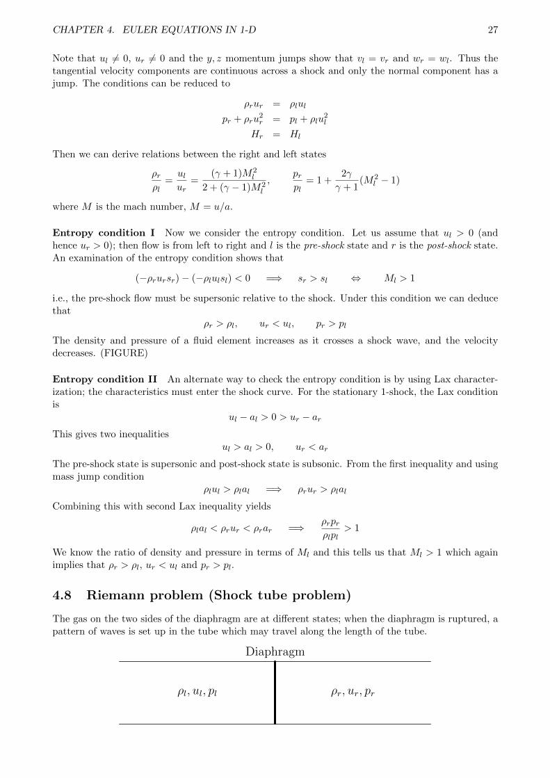
The gas on the two sides of the diaphragm are at different states; when the diaphragm is ruptured, apattern of waves is set up in the tube which may travel along the length of the tube.
Diaphragm
ρl, ul, pl ρr, ur, pr
CHAPTER 4. EULER EQUATIONS IN 1-D 28
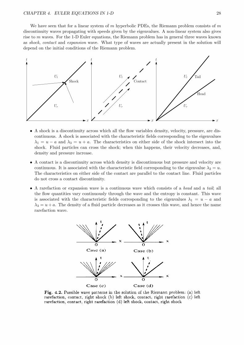
We have seen that for a linear system of m hyperbolic PDEs, the Riemann problem consists of mdiscontinuity waves propagating with speeds given by the eigenvalues. A non-linear system also givesrise to m waves. For the 1-D Euler equations, the Riemann problem has in general three waves knownas shock, contact and expansion wave. What type of waves are actually present in the solution willdepend on the initial conditions of the Riemann problem.
x
t
Shock
Ul
Ur
x
t
Contact
Ul
Ur
x
t
Tail
Head
Ul
Ur
• A shock is a discontinuity across which all the flow variables density, velocity, pressure, are dis-continuous. A shock is associated with the characteristic fields corresponding to the eigenvaluesλ1 = u − a and λ3 = u + a. The characteristics on either side of the shock intersect into theshock. Fluid particles can cross the shock; when this happens, their velocity decreases, and,density and pressure increase.
• A contact is a discontinuity across which density is discontinuous but pressure and velocity arecontinuous. It is associated with the characteristic field corresponding to the eigenvalue λ2 = u.The characteristics on either side of the contact are parallel to the contact line. Fluid particlesdo not cross a contact discontinuity.
• A rarefaction or expansion wave is a continuous wave which consists of a head and a tail; allthe flow quantities vary continuously through the wave and the entropy is constant. This waveis associated with the characteristic fields corresponding to the eigenvalues λ1 = u − a andλ3 = u+ a. The density of a fluid particle decreases as it crosses this wave, and hence the namerarefaction wave.
118 4. The Riemann Problem for the Euler Equations
P(1 - bP) (7 - 1 ) P ’
e = (4.4)
where y is the ratio of specific heats, a constant, and b is the covolume, also a constant. See Sects. 1.2.4 and 1.2.5 of Chap. 1. For the case in which no
Case (a) Case (b)
4 t r t
X
v- \I/I X
0 0
Case (c) Case (d) Fig. 4.2. Possible wave patterns in the solution of the Riemann problem: (a) left rarefaction, contact, right shock (b) left shock, contact, right rarefaction (c) left rarefaction, contact, right rarefaction (d) left shock, contact, right shock
v a c u u m is present the exact solution of the Riemann problem (4.1), (4.2) has three waves, which are associated with the eigenvalues A1 = u - a, A2 = u and A3 = u + a; see Fig. 4.1. Note that the speeds of these waves are not, in general, the characteristics speeds given by the eigenvalues. The three waves separate four constant states, which from left to right are: WL (data on the left hand side), W,L, W,R and WR (data on the right hand side).
The unknown region between the left and right waves, the S t a r Region, is divided by the middle wave into the two subregions S t a r Left (W+L) and S t a r Right (W,R). As seen in Sect. 3.1.3 of Chap. 3, the middle wave is always a contact discontinuity while the left and right (non-linear) waves are either shock or rarefaction waves. Therefore, according to the type of non- linear waves there can be four possible wave patterns, which are shown in Fig. 4.2. There are two possible variations of these, namely when the left or right non-linear wave is a sonic rarefaction wave; these two cases are only of interest when utilising the solution of the Riemann problem in Godunov-type methods. For the purpose of constructing a solution scheme for the Riemann problem it is sufficient t o consider the four patterns of Fig. 4.2.
An analysis based on the eigenstructure of the Euler equations, Sect. 3.1.3 Chap. 3, reveals that both pressure p , and particle velocity u* between the left and right waves are constant, while the density takes on the two constant values p + ~ and p , ~ . Here we present a solution procedure which makes use of the constancy of pressure and particle velocity in the Star Region to derive a
CHAPTER 4. EULER EQUATIONS IN 1-D 29
4.3 Numerical Solution for Pressure 129
2 1.0 -2.0 3 1 .o 0.0 4 1 .o 0.0 5 5.99924 19.5975
4.3.3 Numerical Tests
0.4 1.0 2.0 0.4 1000.0 1.0 0.0 0.01 0.01 1.0 0.0 100.0
460.894 5.99242 -6.19633 46.0950
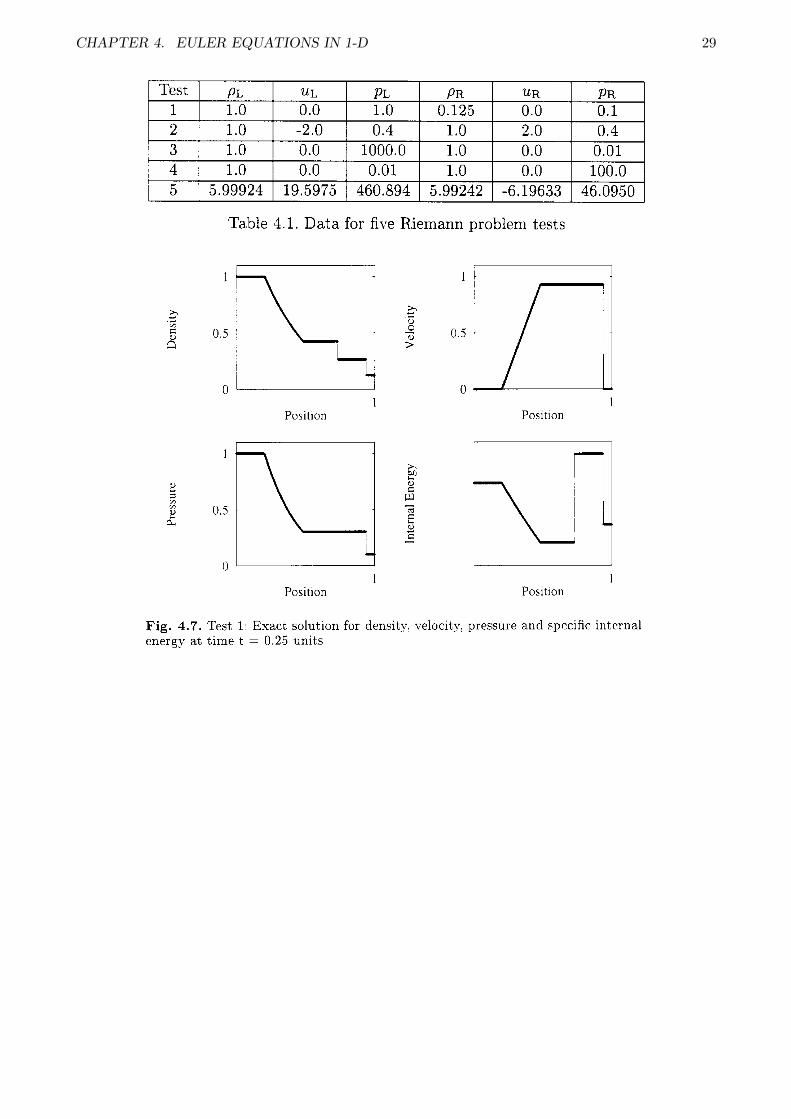
Five Riemann problems are selected to test the performance of the Riemann solver and the influence of the initial guess for pressure. The tests are also used to illustrate some typical wave patterns resulting from the solution of the Riemann problem. Table 4.1 shows the data for all five tests in terms of primitive variables. In all cases the ratio of specific heats is y = 1.4. The source code for the exact Riemann solver, called HE-ElRPEXACT, is part of the library NUMERICA [369]; a listing is given in Sect. 4.9.
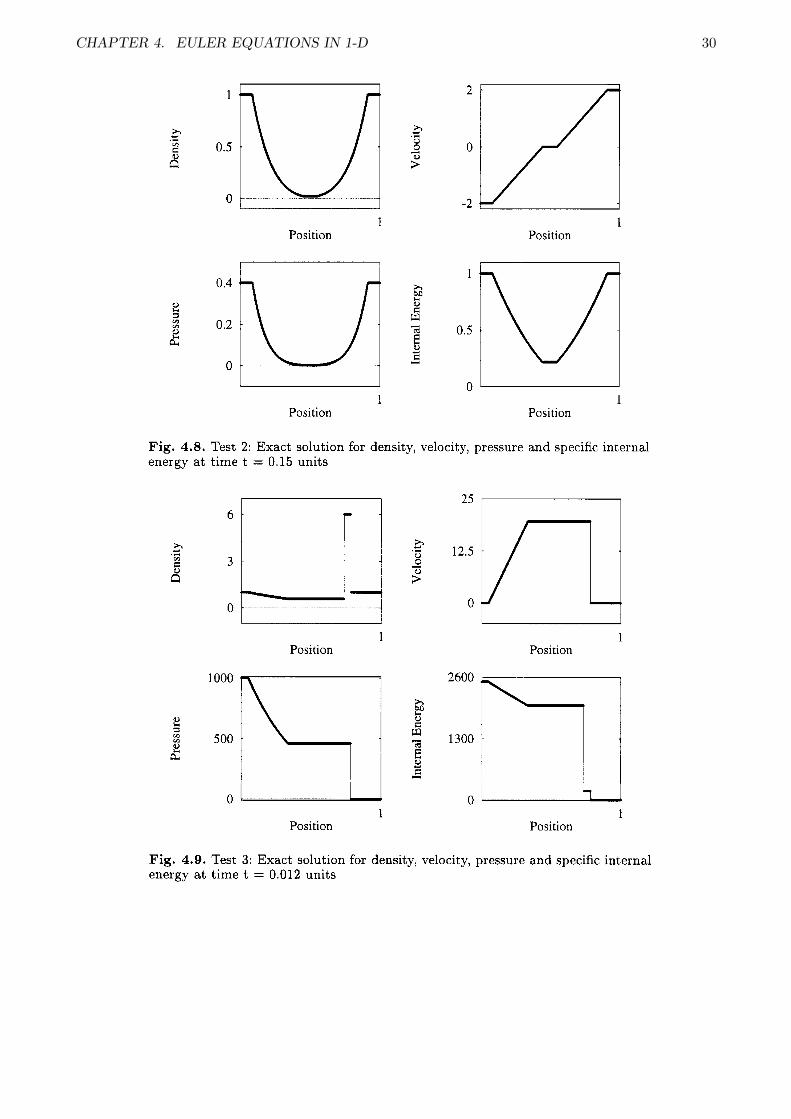
Test 1 is the so called Sod test problem [318]; this is a very mild test and its solution consists of a left rarefaction, a contact and a right shock. Fig. 4.7 shows solution profiles for density, velocity, pressure and specific internal energy across the complete wave structure, at time t = 0.25 units. Test 2, called the 123 problem, has solution consisting of two strong rarefactions and a trivial stationary contact discontinuity; the pressure p , is very small (close to vacuum) and this can lead to difficulties in the iteration scheme to find p , numerically. Fig. 4.8 shows solution profiles. Test 2 is also useful in assessing the performance of numerical methods for low density flows, see Einfeldt et. al. [118]. Test 3 is a very severe test problem, the solution of which contains a left rarefaction, a contact and a right shock; this test is actually the left half of the blast wave problem of Woodward and Colella [413], Fig. 4.9 shows solution profiles. Test 4 is the right half of the Woodward and Colella prob- lem; its solution contains a left shock, a contact discontinuity and a right rarefaction, as shown in Fig. 4.10. Test 5 is made up of the right and left shocks emerging from the solution to tests 3 and 4 respectively; its solution represents the collision of these two strong shocks and consists of a left facing shock (travelling very slowly to the right), a right travelling contact disconti- nuity and a right travelling shock wave. Fig. 4.11 shows solution profiles for Test 5 .
'lkst I pL I UL I P L I PR I UR I PR 1 1 1.0 I 0.0 I 1.0 I 0.125 I 0.0 I 0.1
Table 4.1. Data for five Riemann problem tests
Table 4.2 shows the computed values for pressure in the Star Region by solving the pressure equation f(p) = 0 (equation 4.5) by a Newton-Raphson method. This task is carried out by the subroutine STARPU, which is contained in the FORTRAN 77 program given in Sect. 4.9 of this chapter.
130 4. The Riemann Problem for the Euler Equations
Test 1 2 3 4 5
p, P T R P P V P T S $(PL $- P R ) 0.30313 0.30677(3) 0.55000(5) 0.31527(3) 0.55(5) 0.00189 exact(1) TOL(8) TOL(8) 0.4(9) 460.894 912.449(5) 500.005(4) 464.108(3) 500.005(4) 46.0950 82.9831(5) 50.005(4) 46.4162(3) 50.005(4) 1691.64 2322.65(4) 781.353(5) 1241.21(4) 253.494(6)
Table 4.2 Guess values po for iteration scheme. Next to each guess is the required number of iterations for convergence (in parentheses).
0 1
Position
0 1
Position
0.5 .
0 1
Position
1 Position
Fig. 4.7. Test 1. Exact solution for density, velocity, pressure and specific internal energy a t time t = 0.25 units
The exact. converged. solution for pressure is given in column 2. Columns 3 to 6 give the guess values ~ T R , ppy, p ~ s and the arithmetic mean value of the data. The number in parentheses next to each guess value is the number of iterations required for convergence for a tolerance T O L = l o p 6 . For Test 1. ~ T R and p ~ s are the best guess values for PO. For Test 2 , ~ T R is actually the exact solution (two rarefactions). By excluding Test 2, PTS is the best guess overall. Experience in using hybrid schemes suggests that a combination of two or three approximations is bound t o provide a suitable guess value for po that is both accurate and efficient. In the FORTRAN 77 program provided in Sect. 4.9 of this chapter, the subroutine STARTE contains a hybrid scheme
CHAPTER 4. EULER EQUATIONS IN 1-D 304.3 Numerical Solution for Pressure 131
u .- ; a
e!
e! Le
a
1 Position
1 Position 0,4m 0.2 1 - 0 o . ~ ~
I 0
1 1 Position Position
Fig. 4.8. Test 2: Exact solution for density, velocity, pressure and specific internal energy at time t = 0.15 units
x 4- .- ; a
0 '---1- 1
Position
0 1
Position
1 Position
1300
1 0-
Position
Fig. 4.9. Test 3: Exact solution for density, velocity, pressure and specific internal energy at time t = 0.012 units
4.3 Numerical Solution for Pressure 131
u .- ; a
e!
e! Le
a
1 Position
1 Position 0,4m 0.2 1 - 0 o . ~ ~
I 0
1 1 Position Position
Fig. 4.8. Test 2: Exact solution for density, velocity, pressure and specific internal energy at time t = 0.15 units
x 4- .- ; a
0 '---1- 1
Position
0 1
Position
1 Position
1300
1 0-
Position
Fig. 4.9. Test 3: Exact solution for density, velocity, pressure and specific internal energy at time t = 0.012 units

CHAPTER 4. EULER EQUATIONS IN 1-D 314. The Riemann Problem for the Euler Equations
1 Position
50
10
l o o ! 50 4 10 '
1 Position
-7 - 1
Position
O b 1
Position
Fig. 4.10. Test 4: Exact solution for density, velocity, pressure and specific internal energy at time t = 0.035 units
40
20 x - .C E f r
2000 I I
I Position
1 Position
Fig. 4.11. Test 5: Exact solution for density, velocity, pressure and specific internal energy a t time t = 0.035 units
4. The Riemann Problem for the Euler Equations
1 Position
50
10
l o o ! 50 4 10 '
1 Position
-7 - 1
Position
O b 1
Position
Fig. 4.10. Test 4: Exact solution for density, velocity, pressure and specific internal energy at time t = 0.035 units
40
20 x - .C E f r
2000 I I
I Position
1 Position
Fig. 4.11. Test 5: Exact solution for density, velocity, pressure and specific internal energy a t time t = 0.035 units

Chapter 5
Lax-Friedrich flux
Let us consider a 1-D system of conservation laws
Ut + F (U)x = 0
The central difference schemeUn+1j − Unj
∆t+Fnj+1 − Fnj
2∆x= 0
is unstable for hyperbolic problems. A stable version can be obtained by a small modification
Un+1j − 1
2(Unj−1 + Unj+1)
∆t+Fnj+1 − Fnj
∆x= 0
which can be written in finite volume form with numerical flux
Fj+ 12
=1
2(Fj + Fj+1)− 1
2
∆x
∆t(Uj+1 − Uj)
This has the usual structure
Fj+ 12
=1
2(Fj + Fj+1)− 1
2λ(Uj+1 − Uj), λ =
∆x
∆t= speed
Since the time step must satisfy a CFL condition (show this by Fourier analysis)
∆t = CFL∆x
maxj σ(F ′(Unj )), CFL ≤ 1
where σ is the spectral radius. We see that
λ ≈ maxjσ(F ′(Unj ))
The parameter λ is related to the maximum wave speed in the whole computational domain. Forthis reason, this scheme is also sometimes called global Lax-Friedrich scheme. It is very simple in thesense that we do not need to know anything about the eigenvectors but only need to know the largesteigenvalue. It is a very robust scheme and seldom fails to give an answer, but the results will be verydiffusive.
5.1 Rusanov or local Lax-Friedrich scheme
A simple way to improve the scheme is to use a local estimate of λ so that the flux has the form
Fj+ 12
=1
2(Fj + Fj+1)− 1
2λj+ 1
2(Uj+1 − Uj)
32

CHAPTER 5. LAX-FRIEDRICH FLUX 33
where λj+ 12
is an estimate of the maximum wave speed arising in the Riemann problem at the face
j + 12 . For convex fluxes, a simple choice is
λj+ 12
= maxσ(F ′(Unj )), σ(F ′(Unj+1))
This scheme was proposed by Rusanov [4] and is also called local Lax-Friedrich scheme. For the Eulerequations
λj+ 12
= max|uj |+ aj , |uj+1|+ aj+1
is a good choice.
5.2 Positivity property
Un+1j =
[1− ∆t
2∆x(λj− 1
2+ λj+ 1
2)
]Unj
+λj− 1
2∆t
2∆x
[Uj−1 +
1
λj− 12
Fj−1
]+λj+ 1
2∆t
2∆x
[Uj+1 −
1
λj+ 12
Fj+1
]
=
[1− ∆t
2∆x(λj− 1
2+ λj+ 1
2)
]Unj
+λj− 1
2∆t
2∆xU+j−1 +
λj+ 12∆t
2∆xU−j+1
Theorem 5.1. If U ∈ Uad and λ ≥ |u|+ a then
U± := U ± 1
λF (U) ∈ Uad
Proof. The first component is
ρ± 1
λρu =
1
λρ(λ± u)
≥ 1
λ(|u| ± u+ a)
≥ 1
λa since |u| ± u ≥ 0
> 0
The pressure component is
2
(ρ± 1
λρu
)(E ± 1
λ(E + p)u
)−(ρu± 1
λ(p+ ρu2)
)2
=
Theorem 5.2. The FV scheme with Rusanov flux and λj+ 12
as defined above is positive under the
condition∆t
2∆x(λj− 1
2+ λj+ 1
2) ≤ 1

Chapter 6
Flux Vector Splitting schemes
The main idea is to split the flux F into two parts
F (U) = F+(U) + F−(U)
such that
F+ = due to waves moving to right, positive speed
F− = due to waves moving to left, negative speed
Since eigenvalues determine the wave speeds, we should ensure that
∂F+
∂Uhas positive eigenvalues,
∂F−
∂Uhas negative eigenvalues
Then the numerical flux function is given by
Fi+1/2 = F (Ui, Ui+1) = F+(Ui) + F−(Ui+1)
This is a consistent flux; if Ui = Ui+1 = U
Fi+ 12
= F (U,U) = F+(U) + F−(U) = F (U)
6.1 Steger-Warming scheme
The Steger-Warming flux [6] is based on the homogeneity property of the Euler flux
F (U) = A(U)U, A(U) =∂F
∂U
Split the flux jacobian matrix using eigenvalue splitting
A(U) = A+(U) +A−(U), A±(U) = R(U)Λ±(U)R−1(U)
Then the flux can be split based on eigenvalue splitting
F (U) = A+(U)U +A−(U)U = F+(U) + F−(U) =⇒ F±(U) = A±(U)U
The Steger-Warming flux is given by
Fi+1/2 = F+(Ui) + F−(Ui+1) = A+(Ui)Ui +A−(Ui+1)Ui+1
34

CHAPTER 6. FLUX VECTOR SPLITTING SCHEMES 35
Some properties The flux has the upwind property; e.g., if both Ui, Ui+1 are supersonic to theright, then
A+(Ui) = A(Ui), A−(Ui+1) = 0 =⇒ F (Ui, Ui+1) = A(Ui)Ui = F (Ui)
Moreover, if γ ∈ [1, 5/3]∂F+
∂U≥ 0,
∂F−
∂U≤ 0
It is found to add excessive numerical dissipation and leads to poor resolution of contact waves.Moreover, F± are not differentiable at sonic and stagnation points. Laney recommends smoothingthe eigenvalues
λ±i =1
2
(λi ±
√λ2i + δ2
), i = 1, 2, 3
Implementation A direct implementation can be costly since it involves many matrix-matrix prod-ucts. First express the conserved vector U in terms of the eigenvectors of A
U = α1r1 + α2r2 + α3r3, α1 = α3 =ρ
2γ, α2 = ρ
γ − 1
γ
orU = Rα, α = [α1, α2, α3]>
The split fluxes are given by
F± = A±U = RΛ±R−1(Rα) = RΛ±α = α1λ±1 r1 + α2λ
±2 r2 + α3λ
±3 r3
Remark 6.1. A variant of this flux was proposed by Vijayasundaram [9]
Fi+1/2 = A+(Ui+ 12)Ui +A−(Ui+ 1
2)Ui+1, Ui+ 1
2=
1
2(Ui + Ui+1)
6.2 van Leer splitting
• The Mach number: M = ua tells us about sign of eigenvalues.
• If M > 1: all eigenvalues are positive
M > 1 =⇒ u− a > 0, u > 0, u+ a > 0
and if M < −1, all eigenvalues are negative. We can use the Mach number to determine theupwind direction.
• Euler flux: polynomials in M
F =
ρaMρa2
γ (γM2 + 1)
ρa3M(
12M
2 + 1γ−1
)
• Each component flux of the formF = G(ρ, a)H(M)
Split the flux asF = F+ + F−, F± = G(ρ, a)H±(M)
• Split polynomial H(M) such that we have upwinding and smoothness
1. H(M) = H+(M) +H−(M)
2. H+(M) = 0 for M ≤ −1 ( =⇒ H−(M) = H(M))
3. H+(M) = H(M) for M ≥ 1 ( =⇒ H−(M) = 0)
4. ddMH
+(−1) = 0, ddMH
+(1) = ddMH(1).

CHAPTER 6. FLUX VECTOR SPLITTING SCHEMES 36
6.2.1 van Leer: Mass flux
H(M) = M = M+(M) +M−(M)
• To satisfy all conditions, M± must be quadratic polynomial in M
M+ =
0 M ≤ −1(M+1
2
)2 −1 < M < 1
M M ≥ 1
M− =
M M ≤ −1
−(M−1
2
)2 −1 < M < 1
0 M ≥ 1
6.2.2 van Leer: momentum flux
Split γM2 + 1 using cubic polynomials in M
(γM2 + 1) = (γM2 + 1)+ + (γM2 + 1)−
(γM2 + 1)+ =
0 M ≤ −1(M+1
2
)2[(γ − 1)M + 2] −1 < M < +1
γM2 + 1 M ≥ 1
(γM2 + 1)− =
γM2 + 1 M ≤ −1
−(M−1
2
)2[(γ − 1)M − 2] −1 < M < +1
0 M ≥ 1
6.2.3 van Leer: Energy flux
Split energy flux using quartic polynomials in M
F+3 =
0 M ≤ −1[(γ−1)u+2a]2F+
12(γ+1)(γ−1) −1 < M < 1
F3 M > 1
F−3 =
F3 M ≤ −1[(γ−1)u−2a]2F−
12(γ+1)(γ−1) −1 < M < 1
0 M > 1
6.2.4 van Leer flux
• Final flux formulae
F± = ±1
4ρa(M ± 1)2
1(γ−1)u±2a
γ[(γ−1)u±2a]2
2(γ+1)(γ−1)
• Has upwind property of split flux jacobians
∂F+
∂U≥ 0,
∂F−
∂U≤ 0
• Adds excessive dissipation for contact discontinuity

CHAPTER 6. FLUX VECTOR SPLITTING SCHEMES 37
6.3 Liou and Steffen (1993)
Separate flux into convective and pressure parts
F =
ρup+ ρu2
ρHu
=
ρuρu2
ρHu
+
0p0
= M
ρaρuaρHa
+
0p0
= MFc + Fp
Flux splitting
F± = M±Fc + F±p , F±p =
0p±
0
M± is same as in van Leer scheme. Pressure p = p+ + p−
p+ = p
0 M ≤ −112(1 +M) −1 < M < 1
1 M ≥ 1
, p− = p
1 M ≤ −112(1−M) −1 < M < 1
0 M ≥ 1
Remark: See the papers on AUSM family of schemes.
6.4 Zha-Bilgen flux vector splitting (1993)
F =
ρup+ ρu2
(E + p)u
=
ρuρu2
Eu
+
0ppu
= u
ρρuE
+
0ppu
Flux vector splitting
F± = u±U +
0p±
(pu)±
, u± =1
2(u± |u|)
p± is same as in Liou-Steffen scheme.
(pu)+ = p
0 M ≤ −112(u+ a) −1 < M < 1
u M ≥ 1
, (pu)− = p
u M ≤ −112(u− a) −1 < M < 1
0 M ≥ 1

CHAPTER 6. FLUX VECTOR SPLITTING SCHEMES 38284 8. Flux Vector Splitting Methods
0- 0 0.5 1
Position
0.5
2 B a
I 0
0 0.5 1 Position
1.6 7
0 0 5 1 Position
1.8 1 0 0.5 1
Position
Fig. 8.3. Steger and Warming FVS scheme applied to Test 1, with 20 = 0.3. Numerical (symbol) and exact (line) solutions are compared at time 0.2 units
x I
Y 2 0 5 0
0 0 0 0 5 1 0 0 5 1
Positlon Position
x F 0 5
1 8 0 o s I 0 0 5 I
0
Position
2 a
Positlon
Fig. 8.4. Van Leer FVS scheme applied to Test 1, with 20 = 0.3. Numerical (symbol) and exact (line) solutions are compared at time 0.2 units
284 8. Flux Vector Splitting Methods
0- 0 0.5 1
Position
0.5
2 B a
I 0
0 0.5 1 Position
1.6 7
0 0 5 1 Position
1.8 1 0 0.5 1
Position
Fig. 8.3. Steger and Warming FVS scheme applied to Test 1, with 20 = 0.3. Numerical (symbol) and exact (line) solutions are compared at time 0.2 units
x I
Y 2 0 5 0
0 0 0 0 5 1 0 0 5 1
Positlon Position
x F 0 5
1 8 0 o s I 0 0 5 I
0
Position
2 a
Positlon
Fig. 8.4. Van Leer FVS scheme applied to Test 1, with 20 = 0.3. Numerical (symbol) and exact (line) solutions are compared at time 0.2 units

CHAPTER 6. FLUX VECTOR SPLITTING SCHEMES 398.5 Numerical Results 285
0 0 0.5 1
Position
0 0 0.5 1
Position
1.6
08i? 0
0 0.5 i Position
1.8 - 0 0.5 1
Position
Fig. 8.5. Liou and Steffen scheme applied to Test 1, with 20 = 0.3. Numerical (symbol) and exact (line) solutions are compared at time 0.2 units
0 0.5 1 0 0.5 1 Position Position
0.25 0 ' 5 ~ . f-q I . .-. 0.5 - -
0
0 0 0.5 I 0 0.5 1
Position Position
Fig. 8.6. Steger and Warming FVS scheme applied to Test 2, with 20 = 0.5 . Numerical (symbol) and exact (line) solutions are compared at time 0.15 units

Chapter 7
Godunov scheme
• At any time tn, FV solution is constant in each cell
U(x, tn) = Uni , xi−1/2 < x < xi+1/2
• Riemann problem at every cell interface
• Godunov’s idea
1. Solve Riemann problem for Un at every cell interface exactly
2. Evolve the Riemann solution upto next time level tn+1 = tn + ∆t
3. Average the solution at tn+1 to get cell average values Un+1
• Solution of Riemann problem at xi+1/2
Ui+1/2
(x− xi+1/2
t− tn
)waves moving to left and right
• Waves from successive Riemann problems must not intersect
∆t <h
2Sn
• Sn = maximum wave speed of all Riemann problems
• Average solution at new time level
Un+1i =
1
h
[∫ 12h
0Ui−1/2
(ξ
∆t
)dξ +
∫ 0
− 12hUi+1/2
(ξ
∆t
)dξ
]
• Difficult to implement numerically when expansion waves are present
• CFL condition is more restrictive
• Exact solution of Riemann problem
U(x, t) = Ui+1/2
(x− xi+1/2
t− tn
), xi ≤ x ≤ xi+1, tn ≤ t ≤ tn+1
• Satisfies integral conservation law∫ xi+1/2
xi−1/2
U(x, tn+1)dx =
∫ xi+1/2
xi−1/2
U(x, tn)dx+
∫ ∆t
0F [U(xi−1/2, t)]dt
−∫ ∆t
0F [U(xi+1/2, t)]dt
40

CHAPTER 7. GODUNOV SCHEME 41
But ∫ ∆t
0F [U(xi+1/2, t)]dt =
∫ ∆t
0F [Ui+1/2(0)]dt = F [Ui+1/2(0)]∆t
etc., so that we finally have
Un+1i = Uni −
∆t
h
[F (Ui+1/2(0))− F (Ui−1/2(0))
]• Godunov flux
Fi+1/2 = F (Ui, Ui+1) = F (Ui+1/2(0))
• right moving waves from Ui−1/2 should not reach xi+1/2 and vice versa: CFL condition
∆t <h
Sn
• Accurate but expensive - not used for practical computations
• Recall: Linear system of equations F = AU , A constant matrix
F (Ui+1/2(0)) = A+Ui +A−Ui+1
Here, Godunov scheme is identical to upwind scheme
Chapter 8
Roe scheme
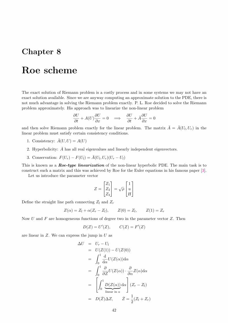
The exact solution of Riemann problem is a costly process and in some systems we may not have anexact solution available. Since we are anyway computing an approximate solution to the PDE, there isnot much advantage in solving the Riemann problem exactly. P. L. Roe decided to solve the Riemannproblem approximately. His approach was to linearize the non-linear problem
∂U
∂t+A(U)
∂U
∂x= 0 =⇒ ∂U
∂t+ A
∂U
∂x= 0
and then solve Riemann problem exactly for the linear problem. The matrix A = A(Ul, Ur) in thelinear problem must satisfy certain consistency conditions.
1. Consistency: A(U,U) = A(U)
2. Hyperbolicity: A has all real eigenvalues and linearly independent eigenvectors.
3. Conservation: F (Ur)− F (Ul) = A(Ul, Ur)(Ur − Ul)
This is known as a Roe-type linearization of the non-linear hyperbolic PDE. The main task is toconstruct such a matrix and this was achieved by Roe for the Euler equations in his famous paper [3].
Let us introduce the parameter vector
Z =
Z1
Z2
Z3
=√ρ
1uH
Define the straight line path connecting Zl and Zr
Z(α) = Zl + α(Zr − Zl), Z(0) = Zl, Z(1) = Zr
Now U and F are homogeneous functions of degree two in the parameter vector Z. Then
D(Z) = U ′(Z), C(Z) = F ′(Z)
are linear in Z. We can express the jump in U as
∆U = Ur − Ul= U(Z(1))− U(Z(0))
=
∫ 1
0
d
dαU(Z(α))dα
=
∫ 1
0
∂
∂ZU(Z(α)) · ∂
∂αZ(α)dα
=
∫ 1
0D(Z(α))︸ ︷︷ ︸linear in α
dα
(Zr − Zl)
= D(Z)∆Z, Z =1
2(Zl + Zr)
42

CHAPTER 8. ROE SCHEME 43
Similarly, we can show for the flux difference
∆F = C(Z)∆Z
The matrices C,D are given by
D(Z) =
2Z1 0 0Z2 Z1 01γZ3
γ−1γ Z2
1γZ1
, C(Z) =
Z2 Z1 0γ−1γ Z3
γ+1γ Z2
γ−1γ Z1
0 Z3 Z2
Hence we have
∆F = A∆U, A = C(Z)D−1(Z)
An explicit computation gives
A =
0 1 0
γ−3γ
(Z2
Z1
)2(3− γ) Z2
Z1γ − 1
γ−12
(Z2
Z1
)3− Z2Z3
Z21
Z3
Z1− (γ − 1)
(Z2
Z1
)2γ Z2
Z1
Define Roe averages
u =Z2
Z1=ul√ρl+ ur√ρr√
ρl+√ρr
, H =Z3
Z1=Hl√ρl+Hr
√ρr√
ρl+√ρr
In terms of these average quantities, the matrix A is
A =
0 1 012(γ − 3)u2 (3− γ)u γ − 1
u[12(γ − 1)u2 − H] H − (γ − 1)u2 γu
Define the average density
ρ =√ρlρr
Define U = conserved vector corresponding to (ρ, u, H). Then
A = A(U)
Hence if we take A = A, all three conditions satisfied. The eigenvalues of A are given by
u− a, u, u+ a
where
a =
√(γ − 1)
[H − 1
2u2
]Let UR(x/t) be the solution of the Riemann problem for the Roe-linearized equation. The flux is givenby F (UR(0)) and we know from linear systems
F (UR(0)) =1
2(Fl + Fr)−
1
2|A(Ul, Ur)|(Ur − Ul)
Moreover, this flux has the upwind property.
Remark 8.1. Show that if the two states Ul, Ur are positive, then the Roe average sound speed a iswell defined.
CHAPTER 8. ROE SCHEME 44
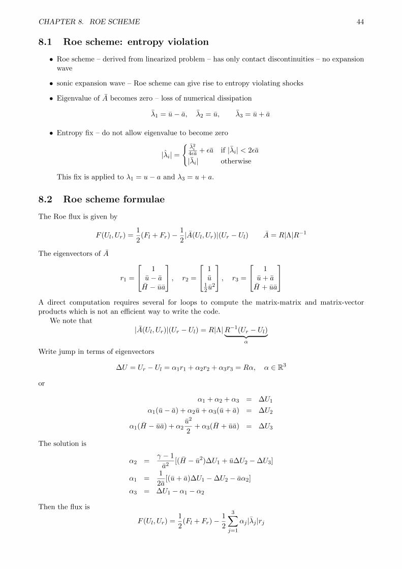
8.1 Roe scheme: entropy violation
• Roe scheme – derived from linearized problem – has only contact discontinuities – no expansionwave
• sonic expansion wave – Roe scheme can give rise to entropy violating shocks
• Eigenvalue of A becomes zero – loss of numerical dissipation
λ1 = u− a, λ2 = u, λ3 = u+ a
• Entropy fix – do not allow eigenvalue to become zero
|λi| =
λ2i4εa + εa if |λi| < 2εa
|λi| otherwise
This fix is applied to λ1 = u− a and λ3 = u+ a.
8.2 Roe scheme formulae
The Roe flux is given by
F (Ul, Ur) =1
2(Fl + Fr)−
1
2|A(Ul, Ur)|(Ur − Ul) A = R|Λ|R−1
The eigenvectors of A
r1 =
1u− aH − ua
, r2 =
1u
12 u
2
, r3 =
1u+ aH + ua
A direct computation requires several for loops to compute the matrix-matrix and matrix-vectorproducts which is not an efficient way to write the code.
We note that|A(Ul, Ur)|(Ur − Ul) = R|Λ|R−1(Ur − Ul)︸ ︷︷ ︸
α
Write jump in terms of eigenvectors
∆U = Ur − Ul = α1r1 + α2r2 + α3r3 = Rα, α ∈ R3
or
α1 + α2 + α3 = ∆U1
α1(u− a) + α2u+ α3(u+ a) = ∆U2
α1(H − ua) + α2u2
2+ α3(H + ua) = ∆U3
The solution is
α2 =γ − 1
a2[(H − u2)∆U1 + u∆U2 −∆U3]
α1 =1
2a[(u+ a)∆U1 −∆U2 − aα2]
α3 = ∆U1 − α1 − α2
Then the flux is
F (Ul, Ur) =1
2(Fl + Fr)−
1
2
3∑j=1
αj |λj |rj
CHAPTER 8. ROE SCHEME 45
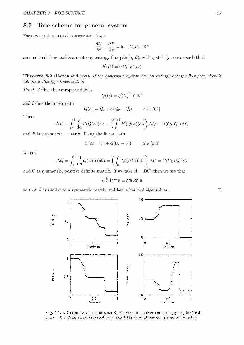
8.3 Roe scheme for general system
For a general system of conservation laws
∂U
∂t+∂F
∂x= 0, U, F ∈ Rn
assume that there exists an entropy-entropy flux pair (η, θ), with η strictly convex such that
θ′(U) = η′(U)F ′(U)
Theorem 8.2 (Harten and Lax). If the hyperbolic system has an entropy-entropy flux pair, then itadmits a Roe-type linearization.
Proof. Define the entropy variablesQ(U) = η′(U)> ∈ Rn
and define the linear pathQ(α) = Ql + α(Qr −Ql), α ∈ [0, 1]
Then
∆F =
∫ 1
0
d
dαF (Q(α))dα =
(∫ 1
0F ′(Q(α))dα
)∆Q = B(Ql, Qr)∆Q
and B is a symmetric matrix. Using the linear path
U(α) = Ul + α(Ur − Ul), α ∈ [0, 1]
we get
∆Q =
∫ 1
0
d
dαQ(U(α))dα =
(∫ 1
0Q′(U(α))dα
)∆U = C(Ul, Ur)∆U
and C is symmetric, positive definite matrix. If we take A = BC, then we see that
C12 AC−
12 = C
12BC
12
so that A is similar to a symmetric matrix and hence has real eigenvalues.11. The Riemann Solver of Roe
I \
L
0 0 0.5 1
Position
i
0 1
0 0.5 I Position
3.8 I
I 0 0.5 I
Position
1.8 ' I 0 0,s 1
Position
Fig. 11.4. Godunov's method with Roe's Riemann solver (no entropy fix) for Test 1, 20 = 0.3. Numerical (symbol) and exact (line) solutions compared at time 0.2
0 0 0.5 1
Position
I I
i. 1 0 I
0 0.5 1 Positlon
O i 0 0 5 1
Position
8 1
1.8 ' 0 0.5 1
Position
Fig. 11.5. Godunov's method with Roe's Riemann solver applied to Test 1, with 20 = 0.3. Numerical (symbol) and exact (line) solutions are compared at time 0.2
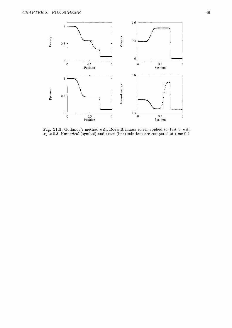
CHAPTER 8. ROE SCHEME 46
11. The Riemann Solver of Roe
I \
L
0 0 0.5 1
Position
i
0 1
0 0.5 I Position
3.8 I
I 0 0.5 I
Position
1.8 ' I 0 0,s 1
Position
Fig. 11.4. Godunov's method with Roe's Riemann solver (no entropy fix) for Test 1, 20 = 0.3. Numerical (symbol) and exact (line) solutions compared at time 0.2
0 0 0.5 1
Position
I I
i. 1 0 I
0 0.5 1 Positlon
O i 0 0 5 1
Position
8 1
1.8 ' 0 0.5 1
Position
Fig. 11.5. Godunov's method with Roe's Riemann solver applied to Test 1, with 20 = 0.3. Numerical (symbol) and exact (line) solutions are compared at time 0.2

Chapter 9
HLL and HLLC Riemann solvers
The Riemann solution for a system gives rise to as many waves as the number of independent variablesin the system. One way to simplify the solution of the Riemann problem is to use a simpler wavemodel where only some waves are included. Clearly, we must include the slowest and fastest wavessince they define the extent of the Riemann solution. We use only simple waves in our model, i.e.,shocks or contact discontinuities.
9.1 HLL Riemann solver
The simplest model is to include only the slowest and fastest waves in the solution [2]. Let us assumethat we have an estimate of these speeds denoted by Sl, Sr with Sl < Sr, and let us consider thesubsonic case
Sl < 0 < Sr
There is one intermediate state which we denote by U∗. (FIGURE) To compute the intermediatestate, let us integrate the conservation law over the space-time region (Sl∆t, Sr∆t)× (0,∆t).∫ ∆t
0
∫ Sr∆t
Sl∆t(Ut + Fx)dxdt = 0
Integrate in t in the first term and x in the second term∫ Sr∆t
Sl∆tU(x,∆t)dx−
∫ Sr∆t
Sl∆tU(x, 0)dx+
∫ ∆t
0[F (Sr∆t, t)− F (Sl∆t, t)]dt = 0
∫ Sr∆t
Sl∆tU∗dx−
∫ 0
Sl∆tUldx−
∫ Sr∆t
0Urdx+
∫ ∆t
0[Fr − Fl]dt = 0
U∗(Sr − Sl)∆t− (0− Sl∆t)Ul − (Sr∆t− 0)Ur + (Fr − Fl)∆t = 0
Canceling ∆t throughout and solving for U∗ yields
U∗ =SrUr − SlUl − (Fr − Fl)
Sr − Sl
What we require for the finite volume scheme is the flux across x = 0 line. Integrate the conservationlaw over the space-time region (Sl∆t, 0)× (0,∆t)∫ ∆t
0
∫ 0
Sl∆t(Ut + Fx)dxdt = 0
∫ 0
Sl∆tU∗dx−
∫ 0
Sl∆tUldx+
∫ ∆t
0[F∗ − Fl]dt = 0
F∗ = Fl + Sl(U∗ − Ul)
47

CHAPTER 9. HLL AND HLLC RIEMANN SOLVERS 48
Alternately, we can integrate over the region (0, Sr∆t)× (0,∆t) to obtain
F∗ = Fr + Sr(U∗ − Ur)
However the two expressions for F∗ yield the same value as can be checked by substituting the expres-sion for U∗
F∗ =SrFl − SlFr + SlSr(Ur − Ul)
Sr − SlNote that F∗ 6= F (U∗) since we have a non-linear conservation law.
Alternate derivation We can write the jump conditions across the two waves Sl, Sr
F∗ − Fl = Sl(U∗ − Ul), Fr − F∗ = Sr(Ur − U∗)
Adding the two equations yields the formula for U∗ and eliminating U∗ from any one of the jumpconditions yields the formula for the flux. This shows that the HLL solver satisfies the jump conditionsacross the two waves.
Numerical flux We have derived the flux for the subsonic case. If 0 < Sl < Sr, then the solutionalong x = 0 is equal to the left state, and conversely if Sl < Sr < 0, then the solution along x = 0 isequal to the right state. Hence, the numerical flux is given by
F (Ul, Ur) =
Fl 0 < Sl < Sr
Fr Sl < Sr < 0
F∗ otherwise
This is a consistent flux and has the upwind property.
9.1.1 Estimation of wave speeds, entropy condition
The only missing information is how to estimate the wave speeds Sl, Sr. We do not know the exactvalues of these speeds Struel , Struer since that would require exact solution of the Riemann problem.Einfeldt et al. suggest the following estimate
Sl = minλ1(Ul), λ1(U), Sr = maxλ1(Ur), λm(U)
where U is the Roe-average state. For the Euler equations, these are given by
Sl = minul − al, u− a, Sr = maxur + ar, u+ a
Theorem 9.1. If the speed estimates satisfy
Sl ≤ Struel , Sr ≥ Struer
i.e., the numerical Riemann fan completely encloses the true Riemann fan, then the entropy conditionis satisfied by the numerical solution.
Remark 9.2. From the above description, we see that the HLL solver can be applied to any system ofconservation laws as long as we can estimate the wave speeds Sl, Sr. No knowledge of the eigenvectorsis required in this solver.
Remark 9.3. If we chooseSl = −λ, Sr = λ
where λ > 0 is the maximum absolute speed in the Riemann problem, then the HLL flux becomes
F∗ =1
2(Fl + Fr)−
1
2λ(Ur − Ul)
which is the Rusanov flux. Thus the Rusanov scheme can be interpreted as an approximate Riemannsolver of HLL-type with Sr = −Sl = λ. However, this scheme is not upwind since the Riemann fan isalways subsonic.

CHAPTER 9. HLL AND HLLC RIEMANN SOLVERS 49
9.1.2 Positivity of intermediate state
9.2 HLLC Riemann solver
The HLL solver does not include the contact wave which is linearly degenerate. Such waves will bedissipated by upwind schemes and they cannot steepen themselves unlike non-linear waves. Henceincluding contact waves in the approximate Riemann solver will enhance the accuracy of solutions. TheHLLC solver [8] uses a wave model with three waves with speeds Sl < S∗ < Sr and two intermediatestates U∗l.U∗r. (FIGURE) The tangential velocity does not change across shocks so that
v∗l = vl, w∗l = wl
v∗r = vr, w∗r = wr
The pressure and normal velocity are continuous across the contact wave
p∗l = p∗r = p∗, u∗l = u∗r = u∗
and the speed of the contact wave coincides with the intermediate velocity S∗ = u∗.The jump conditions across the Sl, Sr waves are
F∗α − Fα = Sα(U∗α − Uα), α = l, r
orF∗α − SαU∗α = Fα − SαUα
or in full ρ∗αu∗
p∗ + ρ∗αu2∗
ρ∗αu∗vαρ∗αu∗wα
(E∗α + p∗)u∗
− Sαρ∗αρ∗αu∗ρ∗αvαρ∗αwαE∗α
=
ραuα
pα + ραu2α
ραuαvαραuαwα
(Eα + pα)uα
− SαραραuαραvαραwαEα
The first jump condition yields
ρ∗α =
(Sα − uαSα − u∗
)ρα (9.1)
With this solution, the third and fourth conditions are satisfied. From the second jump condition
p∗ = pα + ραuα(uα − Sα) + ρ∗αu∗(Sα − u∗)= pα + ραuα(uα − Sα) + ραu∗(Sα − uα) using (9.1)
= pα + ρα(Sα − uα)(u∗ − uα)
We get two estimates of pressure p∗ from the l, r states and equating the two
pl + ρl(Sl − ul)(u∗ − ul) = pr + ρr(Sr − ur)(u∗ − ur)
gives us a formula for u∗
u∗ =ρrur(Sr − ur)− ρlul(Sl − ul)− (pr − pl)
ρr(Sr − ur)− ρl(Sl − ul)
Once u∗ is known, p∗ can be computed using either α = l or α = r. Finally, from the last jumpcondition we obtain
E∗α =1
Sα − u∗[(Sα − uα)Eα + p∗u∗ − pαuα]
This finishes the determination of all the intermediate states and the flux is given by
F (Ul, Ur) =
Fl 0 < Sl
Fr Sr < 0
F∗l = Fl + Sl(U∗l − Ul) Sl < 0 < u∗F∗r = Fr + Sr(U∗r − Ur) u∗ < 0 < Sr

CHAPTER 9. HLL AND HLLC RIEMANN SOLVERS 50
Remark 9.4. To simplify some expressions, we can define
ml = ρl(ul − Sl), mr = ρr(ur − Sr)
Then
u∗ =mrur −mlul − (pr − pl)
mr −ml, p∗ =
mrpl −mlpr +mlmr(ur − ul)mr −ml

Chapter 10
FVM in 1-D: high order schemes
The cell average value is the basic unknown in the finite volume method. If we assume that thesolution is given by piece-wise constant approximation based on cell-averages, then we obtain a firstorder accurate scheme. To obtain higher order accuracy, we can use a more accurate representationof the solution. Let us start with a piece-wise linear approximation in each cell
Ui(x, t) = Ui(t) +1
∆x(x− xi)Si(t), x ∈ Ii+ 1
2
where Si is an approximation to the derivative
1
∆xSi(t) ≈
∂U
∂x(xi, t)
Using this we can evaluate the state at each face
ULi+ 1
2
= Ui +1
2Si, UR
i+ 12
= Ui+1 −1
2Si+1
The semi-discrete finite volume scheme is given by
∆xdUidt
+ Fi+ 12(t)− Fi− 1
2(t) = 0
whereFi+ 1
2(t) = F (UL
i+ 12
(t), URi+ 1
2
(t))
We have a higher order approximation in space and we combine this with a high order time integrationscheme. This is known as method of lines approach.
10.0.1 Second order SSPRK
Stage 1
U (1) = Un − ∆t
∆xR(Un)
Stage 2
Un+1 = U (2) =1
2Un +
1
2
[U (1) − ∆t
∆xR(U (1))
]10.0.2 Third order SSPRK
Stage 1
U (1) = Un − ∆t
∆xR(Un)
Stage 2
U (2) =3
4Un +
1
4
[U (1) − ∆t
∆xR(U (1))
]Stage 3
Un+1 = U (3) =1
3Un +
2
3
[U (2) − ∆t
∆xR(U (2))
]51

CHAPTER 10. FVM IN 1-D: HIGH ORDER SCHEMES 52
10.1 Estimate of reconstruction slope
We have several choices for this based on finite difference formulae
Sbi = Ui − Ui−1, Sfi = Ui+1 − Ui
The reconstructed function must not oscillate and to achieve this, we can choose the smallest of thetwo estimates
Si = minmod(Sbi , Sfi )
where
minmod(a, b) =
smin(|a|, |b|) s = sign(a) = sign(b)
0 otherwise
The total variation of the piece-wise linear reconstruction will not be larger than that of the piece-wiseconstant function. This leads to a very robust method, but it be can rather dissipative at shocks andsmooth extrema.
A small improvement can be made using the central difference estimate
Sci =1
2(Ui+1 − Ui−1)
andSi = minmod(βSbi , S
ci , βS
fi ), β ∈ [1, 2]
where
minmod(a, b, c) =
smin(|a|, |b|, |c|) s = sign(a) = sign(b) = sign(c)
0 otherwise
If β = 1 we obtain the previous scheme. A value of β = 2 is likely to pick the central differenceapproximation and hence gives a more accurate reconstruction, though it might also generate somesmall oscillations.
Remark 10.1. There is huge variety of other schemes to perform the solution reconstruction.
10.2 Local truncation error
Let us study the accuracy in space by substituting a smooth exact solution into the finite volumescheme. If UL
i+ 12
, URi+ 1
2
are obtained from reconstruction using cell averages of the exact solution and
define∆UL
i+ 12
= U(xi+ 12)− UL
i+ 12
, ∆URi+ 1
2
= U(xi+ 12)− UR
i+ 12
Let us assume that the reconstruction is exact for degree k polynomials so that
∆ULi+ 1
2
= O(
∆xk+1), ∆UR
i+ 12
= O(
∆xk+1)
Then
F (ULi+ 1
2
, URi+ 1
2
) = F (U(xi+ 12) + ∆UL
i+ 12
, U(xi+ 12) + ∆UR
i+ 12
)
= F (U(xi+ 12), U(xi+ 1
2)) +
∂
∂UlF (U(xi+ 1
2), U(xi+ 1
2))∆UL
i+ 12
+∂
∂UrF (U(xi+ 1
2), U(xi+ 1
2))∆UR
i+ 12
+O (∆U)2
= F (U(xi+ 12)) +O
(∆xk+1
)+O
(∆x2k+2
)The flux integral term in the scheme has the error
Fi+ 12− Fi− 1
2= F (U(xi+ 1
2))− F (U(xi− 1
2)) +O
(∆xk+1
)

Chapter 11
2-D finite volume method
Consider a 2-D conservation law of the form
Ut + F (U)x +G(U)y = 0
To approximate this by a numerical scheme, we first partition the domain Ω = [xmin, xmax]×[ymin, ymax]by a Cartesian mesh with cells of size ∆x,∆y along the x and y directions respectively. The finitevolume method is however more general and allows the use of non-uniform grids. Let us index thecells by (i, j) and the faces by (i+ 1
2 , j), (i, j + 12), etc., and denote this cell by
Ii,j = [xi− 12, xi+ 1
2]× [yj− 1
2, yj+ 1
2]
and its cell center is (xi, yj). Integrating the conservation law over one cell
d
dt
∫Ii,j
Udxdy+
∫ yj+ 12
∆y
yj− 12
∆y[F (xi+ 1
2, y)− F (xi− 1
2, y)]dy
+
∫ xi+12
∆x
xi− 12
∆x[G(x, yj+ 1
2)−G(x, yj− 1
2)]dx = 0
Define the cell average
Ui,j =1
∆x∆y
∫Ii,j
Udxdy
and the average fluxes
Fi+ 12,j =
1
∆y
∫ yj+ 12
∆y
yj− 12
∆yF (xi+ 1
2, y)dy, Gi,j+ 1
2=
1
∆x
∫ xi+12
∆x
xi− 12
∆xG(x, yj+ 1
2)dx
The semi-discrete takes the form
∆x∆ydUi,jd∆t
+ [Fi+ 12,j − Fi− 1
2,j ]∆y + [Gi,j+ 1
2−Gi,j− 1
2]∆x = 0
We have to still specify how to compute the fluxes which determines the order of accuracy of thescheme.
11.1 First order scheme
Let us consider the solution to be piece-wise constant given by the cell average values. There is a 1-DRiemann problem defined at each point of the vertical faces
Ut + F (U)x = 0, U(x, y, tn) =
Uni,j x < xi+ 1
2
Uni+1,j x > xi+ 12
53

CHAPTER 11. 2-D FINITE VOLUME METHOD 54
from which an approximation to the flux can be obtained.
Fi+ 12,j =
1
∆y
∫ yj+1
2
yj− 1
2
F (Ui,j , Ui+1,j)dy = F (Ui,j , Ui+1,j)
Similarly, at any horizontal face, there is a 1-D Riemann problem
Ut +G(U)y = 0, U(x, y, tn) =
Uni,j y < yj+ 1
2
Uni,j+1 y > yj+ 12
from which an approximation to the flux can be obtained
Gi,j+ 12
= G(Ui,j , Ui,j+1)
We are using 1-D numerical fluxes along x and y directions. Using forward Euler scheme in time, weget the first order finite volume method as
Un+1i,j = Uni,j −
∆t
∆x∆yRni,j
whereRni,j = [Fn
i+ 12,j− Fn
i− 12,j
]∆y + [Gni,j+ 1
2
−Gni,j− 1
2
]∆x
CFL condition A Fourier stability analysis yields the CFL condition
∆t ≤ 1λx∆x +
λy∆y
where λx, λy are maximum wave speeds along the x, y directions in the whole mesh
λx = maxi,j
σ(F ′(Ui,j), λy = maxi,j
σ(G′(Ui,j)
where the maximum is over all the cells in the grid. If ∆x = ∆y = h, λx = λy = λ then
∆t ≤ 1
2
h
λ
and the time step is half the value in 1-D.
Remark 11.1. For Euler equations with velocity components (u, v) and sound speed a, the CFLcondition is given by
∆t ≤ 1
maxi,j
[|ui,j |+ai,j
∆x +|vi,j |+ai,j
∆y
]11.2 Implementation of scheme
11.3 Second order scheme
A second order scheme must have a local truncation error which is O(h2). Another way to characterizea second order scheme is if it is exact for a linear solution. Hence we have to use a piece-wise linearapproximation of the solution inside each cell. The cell average value is a second order approximationto the cell-center value
Ui,j − U(xi, yj) = O(h2)
so we take it as the point value for the purpose of developing the second order scheme.Let us approximate the flux integral by the mid-point rule which is exact for linear functions,
Fi+ 12,j = F (UL
i+ 12,j, UR
i+ 12,j
), Gi,j+ 12
= G(ULi,j+ 1
2
, URi,j+ 1
2
)
CHAPTER 11. 2-D FINITE VOLUME METHOD 55
where ULi+ 1
2,j
etc. are the trace values at the face mid-points obtained by some reconstruction process.
For example
ULi+ 1
2,j
= Ui,j +1
2∆xUi,j , UR
i+ 12,j
= Ui+1,j −1
2∆xUi+1,j
where ∆xUi,j is an estimate of the derivative of U at (xi, yj). The simplest choice is to take
∆xUi,j =1
2[Ui+1,j − Ui−1,j ]
which is second order accurate for smooth functions. But this can lead to oscillations if we are near ashock or steep solution variation. Then some form of non-linear limiter must be used to perform thereconstruction. A simple choice is the minmod reconstruction given by
∆xUi,j = minmod [Ui,j − Ui−1,j , Ui+1,j − Ui,j ]
For scalar problems, this leads to a TVD scheme which eliminates oscillations but the solutions can berather diffused at shocks and smooth extrema since the method becomes first order in those regions.A slightly better version of this scheme is the MC limiter of van Leer given by
∆xUi,j = minmod
[β(Ui,j − Ui−1,j),
1
2(Ui+1,j − Ui−1,j), β(Ui+1,j − Ui,j)
], β ∈ [1, 2]
A larger value of β gives more sharp resolution of shocks, though there may be small oscillations.A similar procedure is used along the y direction. The overall method can be viewed as first
constructing a linear polynomial approximation
Ri,j(x, y) = Ui,j +x− xi
∆x∆xUi,j +
y − yj∆y
∆yUi,j , (x, y) ∈ Ii,j
and using this to get the solution at face mid-points
ULi+ 1
2,j
= Ri,j(xi+ 12, yj), UR
i+ 12,j
= Ri+1,j(xi+ 12, yj)
ULi,j+ 1
2
= Ri,j(xi, yj+ 12), UR
i,j+ 12
= Ri,j+1(xi, yj+ 12)
The high order spatial scheme must be coupled with a high order time integration scheme. For thesecond order scheme, a second or third order SSPRK scheme is a good choice.
Remark 11.2. For second order schemes, it is not necessary to reconstruct conserved variables andwe can use some other set of variables. For Euler equations, the primitive variables are a good choiceas this ensures better control of oscillations. In particular, reconstructing pressure rather than totalenergy can help to ensure positivity of pressure.
11.4 Higher order scheme
To achieve (k + 1)’th order accuracy, i.e., ‖Uexact − Unum‖ = O(∆xk+1
), we must ensure three prop-
erties are satisfied.
1. Reconstruct the solution inside each cell to (k + 1)’th order accuracy. This is satisfied if thereconstruction uses degree k polynomials.
2. Calculate the flux integral using a quadrature rule which is exact for degree k polynomials.
3. Use a (k + 1)’th order accurate time integration scheme.
For second order accuracy (k = 1), we used linear reconstruction and mid-point quadrature, both ofwhich are exact for a linear solution.
CHAPTER 11. 2-D FINITE VOLUME METHOD 56
11.4.1 Solution reconstruction
Our solution is known in terms of cell averages using which we must reconstruct a polynomial insideeach cell.
U(x, y) ≈ Ri,j(x, y), (x, y) ∈ Ii,jWe would like the polynomial Ri,j to have the correct cell average value
1
∆x∆y
∫Ii,j
Ri,j(x, y)dxdy = Ui,j (11.1)
We need more equations to determine the polynomial. E.g., for third order accuracy, we need aquadratic polynomial which has six coefficients. We use an interpolation or least-squares approach tofind the polynomial. For interpolation, we need as many equations as the number of unknowns. Forleast-squares, we use more equations than unknowns. For example, if we use the 3 × 3 cells, we cansolve the following least-squares problem
min∑I∈S
[1
|I|
∫IRi,jdxdy − UI
]2
such that (11.1) is satisfied
whereS = Ii−1,j , Ii+1,j , Ii,j−1, Ii,j+1, Ii−1,j−1, Ii+1,j−1, Ii+1,j+1, Ii−1,j+1
where the constrained minimization is performed wrt the six coefficients in the quadratic polynomial.Of course, we need to implement some form of limiter in case of discontinuous solutions !!!
11.4.2 Flux quadrature
Once the solution is reconstructed in all cells, we can compute the flux integral on cell faces usingsuitable quadrature rule.
Fi+ 12,j =
∑q
F (UL(yq), UR(yq))ωq
where yq are the location of quadrature points on the face, ωq are the quadrature weights, and UL, UR
denote some reconstructions from the left and right cells, respectively.
UL(yq) = Ri,j(xi+ 12, yq), UR(yq) = Ri+1,j(xi+ 1
2, yq)
For third order accuracy, the quadrature must be exact for quadratic polynomials and we could useSimpson rule which has three quadrature points. More efficient methods are based on Gauss-Legendrequadrature; for third order accuracy, 2-point GL quadrature is enough. In generate, the N -point GLquadrature is exact for polynomials of degree upto 2N − 1.

Chapter 12
ENO and WENO schemes
12.1 1-D grid
Given a grid in the domain [a, b]
a = x 12< x 3
2< . . . < xN− 1
2< xN+ 1
2= b
define the cells, cell centers and cell sizes by
Ii = [xi− 12, xi+ 1
2], xi =
1
2(xi− 1
2+ xi+ 1
2), ∆xi = xi+ 1
2− xi− 1
2, i = 1, 2, . . . , N
We denote the maximum cell size by∆x = max
1≤j≤N∆xj
12.2 First order finite volume scheme
For a general conservation law∂u
∂t+∂f
∂x= 0
the semi-discrete finite volume scheme is given by
duidt
+1
∆x[fi+ 1
2− fi− 1
2] = 0
where the numerical flux depends onfi+ 1
2= f(ui, ui+1)
The numerical solution is piecewise constant in each cell, with possible jump at cell interfaces.
12.3 Higher order finite volume scheme
• We know only cell averages, information has been lost in the averaging process.
• Reconstruct solution in each cell by a linear polynomial
pi(x) = ui + (x− xi)si
This preserves cell average value
1
∆x
∫ xi+1
2
xi− 1
2
pi(x)dx = ui
57

CHAPTER 12. ENO AND WENO SCHEMES 58
• How to determine the slope si ?
s−i =ui − ui−1
∆x, s+
i =ui+1 − ui
∆x
Two candidate reconstructions corresponding to above two choices.
• Choose the one with smallest slope (to avoid discontinuities)
si = minmod(s−i , s+i )
where
minmod(a, b) =
smin(|a|, |b|) if s = sign(a) = sign(b)
0 otherwise
• High order in space, semi-discrete scheme
duidt
+1
∆x[fi+ 1
2− fi− 1
2] = 0
wherefi+ 1
2= f(u−
i+ 12
, u+i+ 1
2
)
andu−i+ 1
2
= pi(xi+ 12), u+
i+ 12
= pi+1(xi+ 12)
• Forward Euler time discretization
un+1i = uni −
∆t
∆x[fni+ 1
2
− fni− 1
2
]
• Total variationTV(uh) =
∑i
|ui − ui−1|
• Total variation dimishing property
TV(un+1h ) ≤ TV(unh)
12.4 ENO scheme
• Stencil for reconstruction is chosen adaptively, based on data smoothness
• Extend this idea to higher orders, beyond linear polynomial.
• We need a way to reconstruct solution from cell averages with a high degree polynomial
• This polynomial must be constructed using the smoothest data (stencil)
12.4.1 Polynomial reconstruction
For some smooth function v(x), we are given its cell average values
vi =1
∆xi
∫ xi+1
2
xi− 1
2
v(x)dx
We want to find a polynomial pi(x) of degree at most k − 1 such that it is a k-th order accurateapproximation to v(x), i.e.,
pi(x) = v(x) +O(
∆xk), x ∈ Ii, i = 1, 2, . . . , N
CHAPTER 12. ENO AND WENO SCHEMES 59
We can evaluate this polynomial at the cell boundaries
v+i− 1
2
= pi(xi− 12), v−
i+ 12
= pi(xi+ 12)
which are required to compute the flux in a finite volume method. We want these values to be alsok-th order accurate, i.e.,
v+i− 1
2
= v(xi− 12) +O
(∆xk
), v−
i+ 12
= v(xi+ 12) +O
(∆xk
)12.4.2 Primitive function
Define the primitive function
V (x) =
∫ x
−∞v(ξ)dξ, v(x) =
d
dxV (x)
The lower bound in the above integral can be arbitrarily chosen. Now we know the values of theprimitive function at the cell faces xi+ 1
2since
V (xi+ 12) =
i∑j=−∞
∫ xj+1
2
xj− 1
2
v(ξ)dξ =i∑
j=−∞vj∆xj
Using these known values of V (x), we can construct a polynomial approximation to V (x) of degree atmost k, which we denote by Pi(x), i.e.,
Pi(x) = V (x) +O(
∆xk+1), x ∈ Ii
Then our desired polynomial pi is given by
pi(x) =d
dxPi(x)
12.4.3 Construction of Pj(x)
To construct degree k polynomial, we need k + 1 data points. First note that
V (xi+ 12)− V (xi− 1
2) =
∫ xi+1
2
xi− 1
2
v(x) = vi∆xi
Hence in the construction of Pi(x) we must make use of the values Vi− 12
and Vi+ 12. Let us take the
data at the following k + 1 points
xi−r− 12, . . . , xi+s+ 1
2with r + s+ 1 = k
The polynomial which interpolates this data can be obtained by Lagrange interpolation
Pi(x) =
k∑m=0
V (xi−r+m− 12)
k∏l=0,l 6=m
x− xi−r+l− 12
xi−r+m− 12− xi−r+l− 1
2
12.4.4 Newton form of reconstruction
Define the 0-th divided differenceV [xi− 1
2] := V (xi− 1
2)

CHAPTER 12. ENO AND WENO SCHEMES 60
Then the j-th divided difference, for j ≥ 1 are defined recursively by
V [xi− 12, . . . , xi+j− 1
2︸ ︷︷ ︸j+1 terms
] :=V
j terms︷ ︸︸ ︷[xi+ 1
2, . . . , xi+j− 1
2]−V
j terms︷ ︸︸ ︷[xi− 1
2, . . . , xi+j− 3
2]
xi+j− 12− xi− 1
2
In particular, first divided difference is
V [xi− 12, xi+ 1
2] =
V (xi+ 12)− V (xi− 1
2)
xi+ 12− xi− 1
2
= vi
Let us also define the divided differences of the cell average values by
v[xi] := vi, v[xi, . . . , xi+j ] =v[xi+1, . . . , xi+j ]− v[xi, . . . , xi+j−1]
xi+j − xi
The polynomial Pi interpolating the primitive function V can be written in terms of the Newtondivided differences of V
Pi(x) =k∑j=0
V [xi−r− 12, . . . , xi−r+j− 1
2]
j−1∏m=0
(x− xi−r+m− 12)
Then we obtain pi(x) = P ′i (x) as
pi(x) =k∑j=1
V [xi−r− 12, . . . , xi−r+j− 1
2]
j−1∑m=0
j−1∏l=0,l 6=m
(x− xi−r+l− 12)
Note that only first and higher degree divided differences of V appear in the above expression. Thesecan be written in terms of the divided differences of the cell averages.
12.4.5 Smoothness indicator
How to choose the left shift r and right shift s which determines the stencil for recon-structing the polynomial ? Since we have the freedom to choose the stencil, we would like tochoose it so that the data used in the reconstruction is as smooth as possible. In particular, we wouldlike to avoid choosing data across a shock.
To measure the smoothness of the data, we make use of Newton divided differences. The j-thdivided difference has the property that
V [xi− 12, . . . , xi+j− 1
2] =
V (j)(ξ)
j!, xi− 1
2< ξ < xi+j− 1
2
provided the function V (x) is smooth in this stencil. If V (x) is discontinuous at some point inside thestencil, then it is easy to verify that
V [xi− 12, . . . , xi+j− 1
2] = O
(1
∆xj
)Thus the divided difference is a measurement of the smoothness of the function inside the stencil.
12.5 ENO reconstruction
Our job is to find a stencil of k + 1 consecutive points, which must include xi− 12
and xi+ 12, such that
V (x) is the smoothest in this stencil, compared with other possible stencils.

CHAPTER 12. ENO AND WENO SCHEMES 61
First choose the two point stencil
S2(i) = xi− 12, xi+ 1
2
The linear interpolation on this stencil is
P 1i (x) = V [xi− 1
2] + V [xi− 1
2, xi+ 1
2](x− xi− 1
2)
Next, we have two choices to increase the stencil. If we add the left value xi− 32, then we get
P 2,li (x) = P 1
j (x) + V [xi− 32, xi− 1
2, xi+ 1
2](x− xi− 1
2)(x− xi+ 1
2)
but if we add the right value xi+ 32
we get
P 2,ri (x) = P 1
j (x) + V [xi− 12, xi+ 1
2, xi+ 3
2](x− xi− 1
2)(x− xi+ 1
2)
Among these two quadratic polynomials, we choose the one which has the smallest divided difference.Hence we enhance the stencil as follows
S3(i) =
S2(i) ∪ xi− 3
2, |V [xi− 3
2, xi− 1
2, xi+ 1
2]| < |V [xi− 1
2, xi+ 1
2, xi+ 3
2]|
S2(i) ∪ xi+ 32, otherwise
This procedure is repeated until the stencil contains k + 1 points. Using Sk+1(i) we obtain thepolynomial pi(x) = P ′i (x) which is used to compute
v+i− 1
2
= pi(xi− 12), v−
i+ 12
= pi(xi+ 12)
Finally the flux can be obtained as gi+ 12
= g(v−i+ 1
2
, v+i+ 1
2
) which can be used in a finite volume scheme.
Remark 12.1. Corresponding to each stencil S(i) for primitive function V we have stencil S(i) forconserved variable v. It is enough to build the stencil S(i) to obtain the reconstruction polynomialpi(x).
Remark 12.2. For a uniform grid, it is enough to take undivided differences, which may be useful toavoid roundoff errors.
12.6 TVB property of ENO reconstruction
For a piecewise smooth function V (x), ENO reconstruction starting with the two point stencil S2(i) =xi− 1
2, xi+ 1
2 has following properties:
• The accuracy condition
Pi(x) = V (x) +O(
∆xk+1), x ∈ Ii
is valid for any cell Ii that does not contain a discontinuity. Hence we recover high order accuracyright upto the discontinuity.
• The reconstruction is total variation bounded. That is, there exists a function z(x) satisfying
z(x) = Pi(x) +O(
∆xk+1), x ∈ Ii
for any cell Ii such thatTV (z) ≤ TV (V )
This implies that
TV (pi) ≤ TV (v) +O(
∆xk)

CHAPTER 12. ENO AND WENO SCHEMES 62
12.7 Sign property of ENO scheme
Theorem 12.3 (Fjordholm, Mishra, Tadmor). The ENO reconstruction pi(x) which is a polynomialof degree at most k − 1 satisfies the following sign property
if vi+1 − vi ≥ 0 then v+i+ 1
2
− v−i+ 1
2
≥ 0
if vi+1 − vi ≤ 0 then v+i+ 1
2
− v−i+ 1
2
≤ 0
In particular, if vi = vi+1 then the ENO reconstruction is continuous, i.e., v−i+ 1
2
= v+i+ 1
2
.
12.8 WENO scheme
ENO scheme has some deficiencies.
• The stencil might change due to roundoff errors since we are making a comparison of divideddifferences and choosing the one with the smallest absolute value. The scheme would be non-smooth due to randomly changing stencil from one cell to its neighbour, especially in regionswhere the solution is very smooth or nearly constant.
• Obtaining steady state solutions can be difficult.
• In the stencil selection process, k candidate stencils are considered, covering 2k − 1 cells, butonly one of the stencils is actually used.
• If all the 2k− 1 cells in the potential stencils are used, one could get (2k− 1)-th order accuracyin smooth regions.
12.8.1 Third order approximation for vLi+ 1
2
: k = 2
The candidate stencils are S0 = i, i + 1 and S1 = i − 1, i. (FIGURE) Using S0, find linearpolynomial p0 such that ∫
Ii
p0(x)dx = vi∆x,
∫Ii+1
p0(x)dx = vi+1∆x
If we take p0 of the formp0(x) = vi + (x− xi)s0
then the first condition is already satisfied and we determine s0 from second condition leading to
p0(x) = vi + (x− xi)vi+1 − vi
∆x, v
(0)
i+ 12
= p0(xi+ 12) =
1
2(vi + vi+1) = v(xi+ 1
2) +O
(∆x2
)Similarly using S1, find p1 such that∫
Ii
p1(x)dx = vi∆x,
∫Ii−1
p1(x)dx = vi−1∆x
Hence
p1(x) = vi + (x− xi)vi − vi−1
∆x, v
(1)
i+ 12
= p1(xi+ 12) =
3
2vi −
1
2vi−1 = v(xi+ 1
2) +O
(∆x2
)Using the stencil i − 1, i, i + 1 which is union of stencils S0, S1, construct a quadratic polynomialp(x) such that
1
∆x
∫Ii−1
p(x)dx = vi−1,1
∆x
∫Ii
p(x)dx = vi,1
∆x
∫Ii+1
p(x)dx = vi+1

CHAPTER 12. ENO AND WENO SCHEMES 63
which yields
p(x) = vi + (x− xi)vi+1 − vi−1
2∆x+
[(x− xi)2 − ∆x2
12
]vi−1 − 2vi + vi+1
2∆x2
and
vi+ 12
= p(xi+ 12) = −1
6vi−1 +
5
6vi +
1
3vi+1 = v(xi+ 1
2) +O
(∆x3
)We now try to write the quadratic approximation as a linear combination of the two linear approxi-mations
d0p0(xi+ 12) + d1p1(xi+ 1
2) = p(xi+ 1
2)
−d1
2vi−1 +
d0 + 3d1
2vi +
d0
2vi+1 = −1
6vi−1 +
5
6vi +
1
3vi+1
which has the unique solution
d0 =2
3, d1 =
1
3
12.8.2 Fifth order approximation for vLi+ 1
2
: k = 3
Let us take the candidate stencils as S0 = i, i+ 1, i+ 2, S1 = i− 1, i, i+ 1 and S2 = i− 2, i− 1, iand construct the quadratic polynomial using each stencil. (FIGURE) We evaluate these polynomialsat xi+ 1
2to obtain
v(0)
i+ 12
=1
3vi +
5
6vi+1 −
1
6vi+2 = v(xi+ 1
2) +O
(∆x3
)v
(1)
i+ 12
= −1
6vi−1 +
5
6vi +
1
3vi+1 = v(xi+ 1
2) +O
(∆x3
)v
(2)
i+ 12
=1
3vi−2 −
7
6vi−1 +
11
6vi = v(xi+ 1
2) +O
(∆x3
)Now construct a degree 4 polynomial using i− 2, i− 1, i, i+ 1, i+ 2 = S0 ∪ S1 ∪ S2 and evaluate itat xi+ 1
2
vi+ 12
=1
30vi−2 −
13
60vi−1 +
47
60vi +
9
20vi+1 −
1
20vi+2
We want to choose d0, d1, d2 so that
vi+ 12
= d0v(0)
i+ 12
+ d1v(1)
i+ 12
+ d2v(2)
i+ 12
=d2
3vi−2 −
7d2 + d1
6vi−1 +
2d0 + 5d1 + 11d2
6vi +
2d1 + 5d0
6vi+1 −
d0
6vi+2
The coefficients of vi±2 give
d0 =3
10, d2 =
1
10
We can find d1 from any other coefficient, say vi−1
7d2 + d1
6=
13
60=⇒ d1 =
3
5
We can verify that the above solution matches the coefficients of vi and vi+1 also. Thus we have aunique solution.
CHAPTER 12. ENO AND WENO SCHEMES 64
12.8.3 Non-linear blending
We have seen that each of the small stencils with k cells give an approximation with error O(∆xk
))
v(r)
i+ 12
= pr(xi+ 12) = v(xi+ 1
2) +O
(∆xk
), pr ∈ Pk−1
while the union of all the stencils with 2k − 1 cells gives an approximation of O(∆x2k−1
)vi+ 1
2=∑r
drv(r)
i+ 12
= v(xi+ 12) +O
(∆x2k−1
)The coefficients dr are called linear weights; they are positive and they sum to unity∑
r
dr = 1
We would like to use the high order approximation if the solution in smooth in the larger stencil. Butif there is a shock somewhere in the large stencil, this approximation would not be optimal. In thatcase, it is better to use one of the smaller stencils which does not contain the shock. To achieve thislet us modify the linear weights and write
vi+ 12
=∑r
ωrv(r)
i+ 12
,∑r
ωr = 1
If the solution is smooth in all the stencils then we want ωr ≈ dr so that we get (2k − 1) accuracy.What should be the condition on ωr to achieve this ?∑
r
ωrv(r)
i+ 12
−∑r
drv(r)
i+ 12
=∑r
(ωr − dr)v(r)
i+ 12
−∑r
(ωr − dr)v(xi+ 12)
=∑r
(ωr − dr)(v(r)
i+ 12
− v(xi+ 12))
=∑r
(ωr − dr)O(
∆xk)
= O(
∆x2k−1)
A sufficient condition for the above to hold is
ωr = dr +O(
∆xk−1)
If there is a shock in the r’th stencil, then we want ωr ≈ 0. Due to this requirement, the weights ωrmust depend on the function v which makes the approximation to be non-linear; due to this reasonthe ωr are usually called non-linear weights.
12.8.4 WENO-JS scheme
To measure the smoothness of the polynomials, Jiang and Shu [?] proposed to use a Sobolev normdefined as
βr =
k−1∑l=1
∫ xi+1
2
xi− 1
2
∆x2l−1
(∂lpr(x)
∂xl
)2
dx
and the βr are called smoothness indicators. For third order scheme, the smoothness indicators aregiven by
β0 = (vi+1 − vi)2, β1 = (vi − vi−1)2
while for the fifth order scheme
β0 =13
12(vi − 2vi+1 + vi+2)2 +
1
4(3vi − 4vi+1 + vi+2)2
β1 =13
12(vi−1 − 2vi + vi+1)2 +
1
4(vi−1 − vi+1)2
β2 =13
12(vi−2 − 2vi−1 + vi)
2 +1
4(vi−2 − 4vi−1 + 3vi)
2

CHAPTER 12. ENO AND WENO SCHEMES 65
For smooth solution,
∂lpr(x)
∂xl= O (1) =⇒ βr = O
(∆x2
)+O
(∆x3
)+ . . . = O
(∆x2
)while for discontinuous solution
∂lpr(x)
∂xl= O
(∆x−l
)=⇒ βr = O (1) +O (1) + . . . = O (1)
Jiang and Shu define the non-linear weights as
ωr =αr∑s αs
, αr =dr
(ε+ βr)2, 0 < ε 1
The ε avoids division by zero. Let us consider the fifth order scheme. A Taylor expansion aroundx = xi shows that for smooth solutions
βs = [v′(xi)∆x]2 +O(∆x4
)Solution smooth in all stencils In this case
βs = [v′(xi)∆x]2[1 +O(∆x2
)] =⇒ 1
β2s
=1
[v′(xi)∆x]4[1 +O
(∆x2
)]
and since∑
s ds = 1∑s
αs =∑s
dsβ2s
=1
[v′(xi)∆x]4+O
(∆x−2
)=⇒ 1∑
s αs= [v′(xi)∆x]4[1 +O
(∆x2
)]
Hence
ωr =dr
[v′(xi)∆x]4[1 +O
(∆x2
)]× [v′(xi)∆x]4[1 +O
(∆x2
)] = dr[1 +O
(∆x2
)]
which is sufficient for fifth order accuracy.
Shock in r’th stencil Suppose there is shock in stencil S0 between cell i+ 1 and i+ 2, so that caseβ0 = O (1). Since solution is smooth in S1, S2, then∑
s
αs = O (1) +O(∆x−4
)+O
(∆x−4
)=⇒ 1∑
s αs= O
(∆x4
)[O (1) +O
(∆x4
)] = O
(∆x4
)Hence
ω0 =d0
β20
× 1∑s αs
= O (1)×O(∆x4
)= O
(∆x4
)≈ 0
There is no shock in stencil S2 so that
β2 = O(∆x2
), ω2 =
d2
β22
×O(∆x4
)= O (1)
and similarly, omega1 = O (1). Hence the WENO gives
vi+ 12
= ω0p0(xi+ 12) + ω1p1(xi+ 1
2) + ω2p2(xi+ 1
2) = ω1p1(xi+ 1
2) + ω2p2(xi+ 1
2)
and we get third order accuracy.
Remark 12.4. We can now summarize the WENO algorithm as follows. The third order WENOreconstruction is given by
vLi+ 1
2
= WENO3(vi−1, vi, vi+1)
while the fifth order WENO reconstruction is given by
vLi+ 1
2
= WENO5(vi−2, vi−1, vi, vi+1, vi+2)
Note that the stencil is biased to the left of xi+ 12
in the sense that we have more points on the left of
xi+ 12
than to its right. To compute the values on the right of the face, we can use the same method as
above but pass the correct values; e.g., the fifth order approximation is
vRi+ 1
2
= WENO5(vi+3, vi+2, vi+1, vi, vi−1)

CHAPTER 12. ENO AND WENO SCHEMES 66
12.8.5 Characteristic variable reconstruction
For systems of equations, it is beneficial to apply the reconstruction on characteristic variables ratherthan conserved variables. Locally, characteristic variables are propagated by waves and hence obeysome maximum principle, which is not true for conserved variables. For linear systems, a TVDproperty can be proved if the limiting is applied to characteristic variables. Let U denote the vectorof conserved variables. Compute an average state at the face i+ 1
2 , e.g.,
Ui+ 12
=1
2(Ui + Ui+1)
Compute the matrix of right (Ri+ 12) and left (Li+ 1
2= R−1
i+ 12
) eigenvectors of the flux Jacobian at the
average state and they satisfyRi+ 1
2Li+ 1
2= I
Let us explain how to compute ULi+ 1
2
using the fifth order WENO scheme.
1. Convert conserved to characteristic variables
Wj = W(i+ 1
2)
j = Li+ 12Uj , j ∈ i− 2, i− 1, i, i+ 1, i+ 2, i+ 3
2. Compute WENO reconstruction of each of the characteristic variables1
WLi+ 1
2
= WENO5(Wi−2,Wi−1,Wi,Wi+1,Wi+2)
WRi+ 1
2
= WENO5(Wi+3,Wi+2,Wi+1,Wi,Wi−1)
3. Convert to conserved variables
ULi+ 1
2
= Ri+ 12WLi+ 1
2
, URi+ 1
2
= Ri+ 12WRi+ 1
2
12.9 Example: error convergence
ut + ux = 0, x ∈ (−1,+1)
u(x, 0) = sin(πx)Table 2.2
Accuracy on ut + ux = 0 with u0(x) = sin(πx).
Method N L∞ error L∞ order L1 error L1 order
10 2.98e-2 - 1.60e-2 -
20 1.45e-3 4.36 7.41e-4 4.43
WENO-5 40 4.58e-5 4.99 2.22e-5 5.06
80 1.48e-6 4.95 6.91e-7 5.01
160 4.41e-8 5.07 2.17e-8 4.99
320 1.35e-9 5.03 6.79e-10 5.00
10 4.98e-3 - 3.07e-3 -
20 1.60e-4 4.96 9.92e-5 4.95
CENTRAL-5 40 5.03e-6 4.99 3.14e-6 4.98
80 1.57e-7 5.00 9.90e-8 4.99
160 4.91e-9 5.00 3.11e-9 4.99
320 1.53e-10 5.00 9.73e-11 5.00
Table 2.3
Accuracy on ut + ux = 0 with u0(x) = sin4(πx).
Method N L∞ error L∞ order L1 error L1 order
20 1.08e-1 - 4.91e-2 -
40 8.90e-3 3.60 3.64e-3 3.75
WENO-5 80 1.80e-3 2.31 5.00e-4 2.86
160 1.22e-4 3.88 2.17e-5 4.53
320 4.37e-6 4.80 6.17e-7 5.14
640 9.79e-8 5.48 1.57e-8 5.30
20 5.23e-2 - 3.35e-2 -
40 2.47e-3 4.40 1.52e-3 4.46
CENTRAL-5 80 8.32e-5 4.89 5.09e-5 4.90
160 2.65e-6 4.97 1.60e-6 4.99
320 8.31e-8 5.00 4.99e-8 5.00
640 2.60e-9 5.00 1.56e-9 5.00
In Table 2.2, we show the errors of the fifth order WENO scheme given by the weights (2.58)-(2.59) with the
smooth indicator (2.63), at time t = 1 for the initial condition u0(x) = sin(πx), and compare them with the
errors of the linear 5th order upstream central scheme (referred to as CENTRAL-5 in the following tables).
We can see that fifth order WENO gives the expected order of accuracy starting at about 40 grid points.
In Table 2.3, we show errors for the initial condition u0(x) = sin4(πx). The order of accuracy for the
fifth order WENO settles down later than in the previous example. Notice that this is the example for which
ENO schemes lose their accuracy [63], [67].
We emphasize again that the high order conservative finite difference ENO and WENO schemes of third
or higher order accuracy can only be applied to a uniform grid or a smoothly varying grid, i.e. a grid such
25
N = number of cells, error measured at time t = 1
1We do not show the superscript.
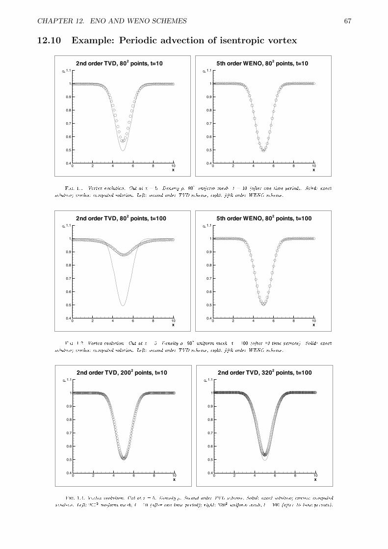
CHAPTER 12. ENO AND WENO SCHEMES 67
12.10 Example: Periodic advection of isentropic vortex
x
ρ
0 2 4 6 8 100.4
0.5
0.6
0.7
0.8
0.9
1
1.12nd order TVD, 802 points, t=10
x
ρ
0 2 4 6 8 100.4
0.5
0.6
0.7
0.8
0.9
1
1.15th order WENO, 802 points, t=10
x
ρ
0 2 4 6 8 100.4
0.5
0.6
0.7
0.8
0.9
1
1.12nd order TVD, 802 points, t=100
x
ρ
0 2 4 6 8 100.4
0.5
0.6
0.7
0.8
0.9
1
1.15th order WENO, 802 points, t=100
x
ρ
0 2 4 6 8 100.4
0.5
0.6
0.7
0.8
0.9
1
1.12nd order TVD, 2002 points, t=10
x
ρ
0 2 4 6 8 100.4
0.5
0.6
0.7
0.8
0.9
1
1.12nd order TVD, 3202 points, t=100
CHAPTER 12. ENO AND WENO SCHEMES 68
12.11 Finite volume WENO in 2-D
12.12 Finite difference WENO scheme
In the finite volume scheme, we reconstruct the solution at the cell face using the cell averages and useany numerical flux function. In the finite difference approach, we assume that we have the solutionat the grid points and we aim to approximate the derivative of the flux at the grid points. This isachieved by reconstructing the flux rather than the solution. The semi-discrete form of the finitedifference scheme is
dvidt
+1
h[fi+ 1
2− fi− 1
2] = 0
The scheme has order of accuracy p if
1
h[fi+ 1
2− fi− 1
2] =
∂f
∂x(xi) +O (hp)
If we had a function F (x) such that
f(x) =1
h
∫ x+h/2
x−h/2F (ξ)dξ
Then∂f
∂x(xi) =
F (xi+ 12)− F (xi− 1
2)
hand we can take
fi+ 12
= F (xi+ 12)
The point value of the flux is
fi = f(xi) =1
h
∫ xi+1
2
xi− 1
2
F (ξ)dξ
is the cell average value of the unknown function F (x) on the i’th cell and this value is known to us.We can apply the WENO idea to construct an approximation to F (xi+ 1
2). However, to obtain a stable
scheme, we must ensure some form of upwinding or correct domain of dependence of the stencil. Forthis purpose let us split the flux into two parts
f = f+ + f−
where∂f−
∂u< 0,
∂f+
∂u> 0
The simplest splitting is given by Lax-Friedrich splitting
f− =1
2[f(u)− λu], f+ =
1
2[f(u) + λu]
whereλ = max
u|f ′(u)|
with the maximum being taken over the range of values of u in our grid or locally at each face. Thesplit fluxes f±
i+ 12
are computed using a WENO scheme. Since f+ represents waves moving with positive
speed, we will use a stencil which is biased towards the left of xi+ 12
to compute this flux, and similarly,
for f−i+ 1
2
we use a stencil which is biased towards the right of xi+ 12. Then the flux will be computed as
fi+ 12
= f+i+ 1
2
+ f−i+ 1
2
Using the fifth order WENO scheme, we can compute the split fluxes as
f+i+ 1
2
= WENO5(f+i−2, f
+i−1, f
+i , f
+i+1, f
+i+2)
f−i+ 1
2
= WENO5(f−i+3, f−i+2, f
−i+1, f
−i , f
−i−1)

CHAPTER 12. ENO AND WENO SCHEMES 69
12.12.1 Analysis of WENO-JS scheme
In this section, we drop the superscript ±. Recall that we have three approximations f ri± 1
2
coming
from quadratic polynomials which are third order accurate
f ri± 1
2
= F (xi± 12) +Ar∆x
3 +O(∆x4
)Their combination with linear weights is fifth order accurate∑
r
drfri± 1
2
= F (xi± 12) +B∆x5 +O
(∆x6
)WENO scheme combines these three values in a non-linear way
fi± 12
=∑r
ω±r fri± 1
2
A Taylor expansion of the smoothness indicators yields
β0 = (f ′i)2∆x2 +
(13
12(f ′′i )2 − 2
3f ′if′′′i
)∆x4 +
(13
6f ′′i f
′′′i −
1
2f ′if′′′′i
)∆x5 +O
(∆x6
)β1 = (f ′i)
2∆x2 +
(13
12(f ′′i )2 +
2
3f ′if′′′i
)∆x4 +O
(∆x6
)β2 = (f ′i)
2∆x2 +
(13
12(f ′′i )2 − 2
3f ′if′′′i
)∆x4 −
(13
6f ′′i f
′′′i −
1
2f ′if′′′′i
)∆x5 +O
(∆x6
)Add and subtract the linear weights
fi± 12
=∑r
drfri± 1
2
+∑r
(ω±r − dr)f ri± 12
=[F (xi± 1
2) +B∆x5 +O
(∆x6
)]+∑r
(ω±r − dr)f ri± 12
since the linear weights are chosen to give fifth order accuracy. The second term is∑r
(ω±r − dr)f ri± 12
=∑r
(ω±r − dr)(F (xi± 1
2) +Ar∆x
3 +O(∆x4
))= F (xi± 1
2)∑r
(ω±r − dr)︸ ︷︷ ︸=0
+∆x3∑r
Ar(ω±r − dr) +
∑r
(ω±r − dr)O(∆x4
)
The first term is zero since the weights sum to unity. The finite difference approximation is
fi+ 12− fi− 1
2
∆x=
F (xi+ 12)− F (xi− 1
2)
∆x+O
(∆x5
)+
∑r(ω
+r − dr)f ri+ 1
2
−∑
r(ω−r − dr)f ri− 1
2
∆x
= f ′(xi) +O(∆x5
)+ ∆x2
∑r
Ar(ω+r − ω−r )
+∑r
(ω+r − dr)O
(∆x3
)−∑r
(ω−r − dr)O(∆x3
)In case of smooth function, the WENO-JS weights satisfy
ω±r = dr +O(∆x2
)then the last two terms are of O
(∆x5
).Using Taylor expansions we can show that
∆x2∑r
Ar(ω+r − ω−r ) = O
(∆x5
)and hence we get fifth order accuracy

CHAPTER 12. ENO AND WENO SCHEMES 70
12.12.2 WENO-Z scheme
The discussion of the WENO-JS scheme shows that the conclusions are not valid if v′(xi) = 0, i.e., wehave a local extremum at x = xi. Let us assume this is the case but also that f ′′i 6= 0. Then
β0 = β2 =13
12[f ′′i ∆x2]2[1 +O (∆x)], β1 =
13
12[f ′′i ∆x2]2[1 +O
(∆x2
)]
This leads toω0 = d0 +O (∆x) , ω2 = d2 +O (∆x)
so that
∆x2∑r
Ar(ω+r − ω−r ) = ∆x2
∑r
Ar(ω+r − dr + dr − ω−r ) = ∆x2O (∆x) = O
(∆x3
)and we get only third order accuracy.
A modification of the non-linear weights was proposed in [1] to take care of such extrema. Define
τ = |β0 − β2|
If solution is smooth in all stencils then
τ =13
3|f ′′i f ′′′i |∆x5 +O
(∆x6
)Define smoothness indicators as
βzr =βr + ε
βr + τ + ε, 0 < ε 1
Then the nonlinear weights are given by
ωr =αr∑s αs
, αs =dsβzs
= ds
(1 +
τ
βs + ε
)The WENO-Z scheme yields fifth order accuracy even at smooth extrema.
12.13 Central WENO (CWENO) schemes
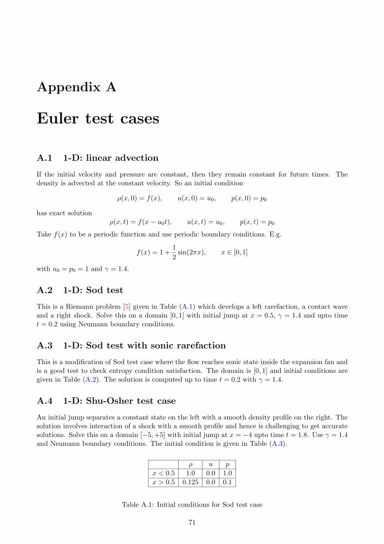
Appendix A
Euler test cases
A.1 1-D: linear advection
If the initial velocity and pressure are constant, then they remain constant for future times. Thedensity is advected at the constant velocity. So an initial condition
ρ(x, 0) = f(x), u(x, 0) = u0, p(x, 0) = p0
has exact solutionρ(x, t) = f(x− u0t), u(x, t) = u0, p(x, t) = p0
Take f(x) to be a periodic function and use periodic boundary conditions. E.g.
f(x) = 1 +1
2sin(2πx), x ∈ [0, 1]
with u0 = p0 = 1 and γ = 1.4.
A.2 1-D: Sod test
This is a Riemann problem [5] given in Table (A.1) which develops a left rarefaction, a contact waveand a right shock. Solve this on a domain [0, 1] with initial jump at x = 0.5, γ = 1.4 and upto timet = 0.2 using Neumann boundary conditions.
A.3 1-D: Sod test with sonic rarefaction
This is a modification of Sod test case where the flow reaches sonic state inside the expansion fan andis a good test to check entropy condition satisfaction. The domain is [0, 1] and initial conditions aregiven in Table (A.2). The solution is computed up to time t = 0.2 with γ = 1.4.
A.4 1-D: Shu-Osher test case
An initial jump separates a constant state on the left with a smooth density profile on the right. Thesolution involves interaction of a shock with a smooth profile and hence is challenging to get accuratesolutions. Solve this on a domain [−5,+5] with initial jump at x = −4 upto time t = 1.8. Use γ = 1.4and Neumann boundary conditions. The initial condition is given in Table (A.3).
ρ u p
x < 0.5 1.0 0.0 1.0
x > 0.5 0.125 0.0 0.1
Table A.1: Initial conditions for Sod test case
71

APPENDIX A. EULER TEST CASES 72
ρ u p
x < 0.3 1.0 0.75 1.0
x > 0.3 0.125 0.0 0.1
Table A.2: Initial conditions for modified Sod test case with sonic rarefaction
ρ u p
x < −4 3.857143 2.699369 10.33333
x > −4 1.0 + 0.2 sin(5x) 0.0 1.0
Table A.3: Initial conditions for Shu-Osher test case
A.5 1-D: 123 problem
The initial condition is given by [7]
(ρ, u, p) =
(1.0, −2.0, 0.4) x < 0.5
(1.0, +2.0, 0.4) x > 0.5
The computational domain is [0, 1] and the final time is t = 0.15. The density becomes very small inthe middle of the domain and can be challenging test in terms of maintaining positive density.
A.6 1-D: Interaction of blast waves
The problems involves interaction of two shock waves and the initial condition is given by [10]
(ρ, u, p) =
(1.0, 0.0, 1000.0) x < 0.1
(1.0, 0.0, 0.01) 0.1 < x < 0.9
(1.0, 0.0, 100.0) x > 0.9
The domain can be taken as [0, 1] and the computations performed upto the time t = 0.038. Solidwall boundary conditions are used on both end points of the domain.
A.7 2-D: Isentropic vortex
The flow consists of a vortex that moves with a constant speed [11]. The initial condition is given by
ρ =
[1− (γ − 1)β2
8γπ2exp(1− r2)
]1/(γ−1)
u = M cosα− β
2πexp(1
2(1− r2))(y − y0)
v = M sinα+β
2πexp(1
2(1− r2))(x− x0)
p = ργ
wherer2 = (x− x0)2 + (y − y0)2
Here (x0, y0) is the center of the vortex. The vortex moves at an angle α to the x axis at a constantspeed of M . The flow has constant entropy everywhere and for all times.
Take a domain of [−5,+5]× [−5,+5] with these parameters
(x0, y0) = (0, 0), β = 5, M = 0.5, α = π/4
Use periodic boundary conditions and run up to a time of t = 10√
2/M ; the vortex would have comeback to its initial position. Note that for high order methods, it is better to use a larger domain sincethe exponential functions may not have decayed at the boundary.

APPENDIX A. EULER TEST CASES 73
A.8 2-D: Shock reflection
This problem consist of a shock which hits the bottom wall and gets reflected and the flow eventuallyreaches a steady state. The domain is [0, 4]× [0, 1] and the initial condition can be taken as
ρ = 1, (u, v) = (2.9, 0.0), p = 1/γ
with γ = 1.4. The flow enters the domain from the left and top sides. The conditions at the left sideare same as the above initial conditions while the conditions on the top are
ρ = 1.69997, (u, v) = (2.61934,−0.50632), p = 1.52819
The botton side is a solid wall and we can use Neumann conditions on the right side.

Bibliography
[1] R. Borges, M. Carmona, B. Costa, and W. S. Don, An improved weighted essentiallynon-oscillatory scheme for hyperbolic conservation laws, Journal of Computational Physics, 227(2008), pp. 3191–3211.
[2] A. Harten, P. D. Lax, and B. van Leer, On Upstream Differencing and Godunov-TypeSchemes for Hyperbolic Conservation Laws, SIAM Review, 25 (1983), pp. 35–61.
[3] P. L. Roe, Approximate Riemann solvers, parameter vectors, and difference schemes, Journal ofComputational Physics, 43 (1981), pp. 357–372.
[4] V. Rusanov, The calculation of the interaction of non-stationary shock waves and obstacles,USSR Computational Mathematics and Mathematical Physics, 1 (1962), pp. 304–320.
[5] G. A. Sod, A survey of several finite difference methods for systems of nonlinear hyperbolicconservation laws, Journal of Computational Physics, 27 (1978), pp. 1–31.
[6] J. L. Steger and R. Warming, Flux vector splitting of the inviscid gasdynamic equations withapplication to finite-difference methods, Journal of Computational Physics, 40 (1981), pp. 263–293.
[7] E. F. Toro, Riemann Solvers and Numerical Methods for Fluid Dynamics, Springer BerlinHeidelberg, Berlin, Heidelberg, 2009.
[8] E. F. Toro, M. Spruce, and W. Speares, Restoration of the contact surface in the HLL-Riemann solver, Shock Waves, 4 (1994), pp. 25–34.
[9] G. Vijayasundaram, Transonic flow simulations using an upstream centered scheme of Godunovin finite elements, Journal of Computational Physics, 63 (1986), pp. 416–433.
[10] P. Woodward and P. Colella, The numerical simulation of two-dimensional fluid flow withstrong shocks, Journal of Computational Physics, 54 (1984), pp. 115–173.
[11] H. Yee, N. Sandham, and M. Djomehri, Low-Dissipative High-Order Shock-Capturing Meth-ods Using Characteristic-Based Filters, Journal of Computational Physics, 150 (1999), pp. 199–238.
74