Numerical Methods and Volatility Models

for Valuing Cliquet Options

H.A. Windcliff∗, P.A. Forsyth†, and K.R. Vetzal‡

Revised: February 14, 2006First Version: September 13, 2004

Abstract

Several numerical issues for valuing cliquet options using PDE methods are investigated.The use of a running sum of returns formulation is compared to an average return formulation.Methods for grid construction, interpolation of jump conditions, and application of boundaryconditions are compared. The effect of various volatility modelling assumptions on the valueof cliquet options is also studied. Numerical results are reported for jump diffusion models,calibrated volatility surface models, and uncertain volatility models.

Keywords: Cliquet options, jump diffusion, interpolation, boundary conditions, volatility mod-els

AMS Classification: 65M12, 65M60, 91B28

Acknowledgment: This work was supported by the Natural Sciences and Engineering Re-search Council of Canada, RBC Financial Group, and a subcontract with Cornell University,Theory & Simulation Science & Engineering Center, under contract 39221 from TG InformationNetwork Co. Ltd.

1 Introduction

Cliquet options are financial derivative contracts which provide a guaranteed minimum annualreturn in exchange for capping the maximum return earned each year over the life of the contract.Recent turmoil in financial markets has led to a demand for products that reduce downside riskwhile still offering upside potential.1 For example, pension plans have been looking at attachingguarantees to their products that are linked to equity returns. Some plans, such as those described∗Equity Trading Lab, Morgan Stanley, 1585 Broadway Ave, 9th Floor, New York, NY 10036, (e-mail:

Heath.Windcliff@morganstanley.com).†School of Computer Science, University of Waterloo, 200 University Ave West, Waterloo ON, Canada N2L 3G1

(e-mail: paforsyt@elora.uwaterloo.ca).‡Centre for Advanced Studies in Finance, University of Waterloo, 200 University Ave West, Waterloo ON, Canada

N2L 3G1 (e-mail: kvetzal@watarts.uwaterloo.ca).1See “Selling Pessimism”, The Economist, March 8, 2003, for related discussion.

1

by Walliser (2003), limit the upside returns in order to reduce the costs associated with providingthe guarantee. These products are essentially cliquet contracts.

Wilmott (2002) illustrated that cliquet options are sensitive to the model assumed for the un-derlying asset dynamics. In this paper we will explore a variety of modelling alternatives, including:

• a (finite activity) jump diffusion model (Merton, 1976);

• a state-dependent volatility surface (i.e. a model in which a local volatility function is cali-brated to observed market prices of traded options, as described, for example, in Colemanet al. (1999)); and

• a nonlinear uncertain volatility model (Avellaneda et al., 1995; Lyons, 1995).2

We find that even if a time-dependent and state-dependent local volatility model is calibratedto prices of plain vanilla options generated from a jump diffusion model with constant parameters,there is no guarantee that the values of cliquet options calculated using the volatility surface willbe close to cliquet values obtained using the jump diffusion model. This result is consistent withother studies, see e.g. Hirsa et al. (2003); Schoutens et al. (2004), which have demonstrated that amodel calibrated to vanilla options does not necessarily price exotics correctly.

However, some practitioners are aware that simply using the local volatility surface calibratedto vanillas does not correctly capture the dynamics of the skew. Practitioners often attempt tomake up for the known deficiencies of a calibrated local volatility surface by forcing the surface tobe homogeneous of degree zero in price and strike. In addition, the surface is often rolled forwardin time. It appears that previous studies have not taken into account these typical corrections.

Assuming that the true market process is a jump diffusion, we show that these two commoncorrections can result in much less error for the price of a cliquet option (at the initial value of theunderlying asset). This provides some justification for common industry practice. However, theerror is small only when the underlying is at the initial price. Consequently, the deltas computedusing the local volatility surface are considerably in error.

Cliquets are discretely observed path-dependent contracts. As such, they can be convenientlyvalued by solving a set of one dimensional PDEs embedded in a higher dimensional space. Theseone dimensional PDEs exchange information through no-arbitrage jump conditions on observationdates. Wilmott (1998) has recommended this approach as a general framework and it has success-fully been used to implement models for Parisian options (Vetzal and Forsyth, 1999), Asian options(Zvan et al., 1999), shout options (Windcliff et al., 2001), volatility swaps and options (Windcliff,Forsyth, and Vetzal, Windcliff et al.), and many others.

An important focus of this paper is to develop effective numerical methods for valuing cliquetoptions for all of the above models. Assuming we have effective methods for solving each onedimensional problem, there are still difficulties in solving the full cliquet problem. In particular,we will:

• show how the use of scaled grids for each one dimensional problem dramatically improves theconvergence;

2Note that this was suggested by Wilmott (2002), who observed that the volatility risk for cliquet options istypically underestimated.

2

• investigate the effects of interpolation methods used to enforce the jump conditions arisingfrom the state variable updating rules;

• show how to specify the boundary conditions at large and small values of the asset price; and

• look at the effects of using a finite computational domain on the data needed to enforce thejump conditions.

We will also compare the performances of a formulation that utilizes a running sum of returns withone that uses the running average of returns.

We emphasize that although the numerical techniques illustrated in this paper will be studiedin conjunction with cliquet options, many of these methods also apply to other path-dependentoptions. For example, the interpolation and grid construction techniques described in this papercan also be used to dramatically improve the performance of algorithms for valuing discretelyobserved floating strike lookback options.

2 Formulation for Jump Diffusion and Uncertain Volatility Mod-els

Let S represent the price of the underlying asset. The potential paths followed by S can be modelledby a stochastic differential equation given by

dS

S= (ξ − λκ)dt+ σdz + (η − 1)dq, (2.1)

where ξ is the drift rate, dq is an independent Poisson process with mean arrival time λ (i.e. dq = 1with probability λdt and dq = 0 with probability 1−λdt), (η−1) is an impulse function producinga jump from S to Sη, κ is the expected value of (η − 1), σ is the volatility (of the continuous partof the process), and dz is the increment of a standard Gauss-Wiener process.

Let V (S, t) be the value of a European-style contract that depends on the underlying asset valueS and time t. Following standard arguments (see, e.g. Merton, 1976; Wilmott, 1998; Andersen andAndreasen, 2000), the following backward partial integro differential equation (PIDE) for the valueof V (S, τ) is obtained

Vτ =σ(Γ, S, t)2S2

2VSS + (r − λκ)SVS − rV +

(λ

∫ ∞0

V (Sη)g(η)dη − λV), (2.2)

where τ = T − t, T is the maturity date of the contract, Γ = VSS , r is the risk free rate of interest,and g(η) is the probability density function of the jump amplitude η. In this paper, we will followMerton (1976) and assume that η is lognormally distributed with mean µ and standard deviationγ, so that κ = exp(µ+ γ2/2)− 1. Specifically

g(η) =e

(− (log(η)−µ)2

2γ2

)√

2πγη. (2.3)

3

In equation (2.2) we have allowed the volatility to be a function of Γ = VSS , as well as theunderlying asset price, S, and time, t. In an uncertain volatility model (Avellaneda et al., 1995;Lyons, 1995), it is assumed that

σmin ≤ σ ≤ σmax (2.4)

but is otherwise uncertain. The worst case value for an investor with a long position in the optionis determined from the solution to equation (2.2) with σ(Γ) given by

σ(Γ)2 =

σ2

max if Γ < 0σ2

min if Γ > 0. (2.5)

Conversely, the best case value for an investor with a long position is determined from the solutionto equation (2.2) with σ(Γ) given by

σ(Γ)2 =

σ2

max if Γ > 0σ2

min if Γ < 0. (2.6)

The worst case value for an investor with a short position (a negative payoff) in the option is givenby the negative of the solution to equations (2.2) and (2.6). Consequently, as discussed in Forsythand Vetzal (2001), the worst-best case long values can be thought of as corresponding to the bid-askprices for the option if buyers and sellers value it assuming worst case scenarios from their ownperspectives.

3 Local Volatility Models

In this section, we postulate a synthetic market where the price process is a jump diffusion withconstant parameters, as in equation (2.1). We then take the point of view of a practitioner whoattempts to fit observed vanilla option prices using a local volatility model. We first develop someanalytic results which provide some insight into the form of the fitted local volatility model. Then,we generate two local volatility surfaces which will be used in the subsequent numerical tests.

3.1 Overview

It is common practice to fit a local volatility model to vanilla option prices, and then use this localvolatility surface to price exotic options. In this section, we will determine some properties of alocal volatility model (no jumps) which has been calibrated to prices in a synthetic market wherethe price process is a constant volatility jump diffusion model.

Suppose that the asset in the synthetic market follows

dS

S= (ξ − λκ)dt+ σJdz + (η − 1)dq, (3.1)

where we assume that for simplicity that σJ = const., and that the jump size distribution g(η) isindependent of (S, t), and given by equation (2.3).

4

If we assume the process (3.1), then the value of an option V given by (2.2) can be written inthe form

Vτ =σ2JS

2

2VSS + rSVS − rV + λ

∫ ∞0

([V (Sη)− V (S)]− (η − 1)SVS

)g(η) dη. (3.2)

Now, suppose the real world process follows the jump diffusion (3.1), but a practitioner assumesthat stock prices evolve according to

dS

S= νdt+ σL(S, t)dz, (3.3)

where ν is the drift term and σL is the local volatility. Let W be the price of an option obtainedassuming process (3.3). W satisfies

Wτ =σL(S, t)2S2

2WSS + rSWS − rW. (3.4)

Typically, the local volatility is determined by calibration to a set of vanilla option prices forfixed (S, t), with varying strikes and maturities (K,T ). Let V (S, t;K,T ) be the price of a vanillacall valued under process (3.1). The price can be regarded as a function of (S, t) with (K,T ) fixedor as a function of (K,T ) with (S, t) fixed. Using the latter perspective, we will let S = S∗, t = t∗ toemphasize that we regard (S∗, t∗) as fixed. Andersen and Andreasen (2000) show that the forwardPIDE for a European call option is

VT =σ2JK

2

2VKK − rKVK

+ λ

∫ ∞0

[ηV (S∗, t∗;K/η, T )− ηV (S∗, t∗;K,T ) + (η − 1)KVK

]g(η)dη. (3.5)

The boundary conditions for equation (3.5) are

V (S∗, t∗; 0, T ) = S∗

V (S∗, t∗;K →∞, T ) = 0V (S∗, t∗;K, t∗) = max(S∗ −K, 0). (3.6)

Let W (S∗, t∗;K,T ) be the price of a European call obtained assuming process (3.3). As shownin Dupire (1994), the forward PDE for W satisfies

WT =σL(K,T )2K2

2WKK − rKWK . (3.7)

We will first consider the solution of the forward equation (3.7) on the finite domain Ωf =[Kmin,Kmax]. We will assume as well that S∗ ∈ Ωf . We will also consider expiry times T boundedaway from t∗, i.e. T ∈ [Tmin, Tmax], Tmin > t∗. After carrying out an analysis in the finite domainΩf × [Tmin, Tmax], we will take limits as Tmin → t∗, Kmin → 0, and Kmax →∞.

The calibration problem can then be stated as follows. Given V (S∗, t∗;K,T ) satisfying initialconditions (3.6) in 0 ≤ K ≤ ∞, t∗ ≤ T ≤ Tmax, determine σL(S∗, t∗;K,T ) such that W = V in

5

Ωf×[Tmin, Tmax]. In other words, determine the local volatility function such that the market pricesfor vanilla calls V are matched by the calibrated prices W at a specific (S∗, t∗), for all strikes andmaturities in Ωf × [Tmin, Tmax]. Note that we have emphasized that the solution to the calibrationproblem σL = σL(S∗, t∗;K,T ) is in general valid only for a specific (S∗, t∗).

For future reference, at this point we gather together some conditions on the solutions for V,W :

Conditions 3.1 (Conditions on V ) We assume the following conditions for V , the solution toequation (3.5) in the domain 0 ≤ K ≤ ∞, t∗ ≤ T ≤ Tmax:

• Initial conditions (T = t) and boundary conditions are given by equation (3.6).

• σ2J > 0 in equation (3.5).

• V has bounded and continuous derivatives of up to first order in T and second order in K inΩf × [Tmin, Tmax] (i.e. V is C1,2).

• VKK > 0 in Ωf × [Tmin, Tmax].

Conditions 3.2 (Conditions on W ) We assume the following conditions for W , the solution toequation (3.7) in the domain Ωf × [Tmin, Tmax]:

• Given a solution V to equation (3.5), initial conditions and boundary conditions for W are

W (S∗, t∗;K,Tmin) = V (S∗, t∗;K,Tmin)W (S∗, t∗;Kmax, T ) = V (S∗, t∗;Kmax, T )W (S∗, t∗;Kmin, T ) = V (S∗, t∗;Kmin, T ). (3.8)

• σ2L > 0 in Ωf × [Tmin, Tmax].

• W has bounded and continuous derivatives of up to first order in T and second order in K(i.e. W is C1,2).

Remark 3.1 Clearly, as T → t∗, then the initial condition (3.6) implies that VKK = 0 for K 6= S.However, for any Tmin > t∗, VKK > 0 in Ωf × [Tmin, Tmax].

Let E = W − V and subtract equation (3.5) from equation (3.7) to obtain

LE = f(S∗, t∗;K,T )

f(S∗, t∗;K,T ) = −(σ2J − σ2

L

2

)K2VKK

− λ∫ ∞

0

(ηV (S∗, t∗;K/η, T )− ηV (S∗, t∗;K,T ) + (η − 1)KVK

)g(η)dη, (3.9)

where

LE ≡ ET −[σ2LK

2

2EKK − rKEK

]. (3.10)

6

From equation (3.8) we have

E(K,T ) = 0, K ∈ ∂Ωf , T ∈ [Tmin, Tmax],E(K,Tmin) = 0, K ∈ Ωf . (3.11)

Consequently, the calibration problem may be restated as: find σL(S∗, t∗;K,T ) such that E = 0 inΩf × [Tmin, Tmax].

If σ2L > 0 in equation (3.10), then the Green’s function (Roach, 1982; Garroni and Menaldi,

1992) of L is the solution to

LG = δ(K −K ′)δ(T − T ′)G(K,T ) = 0, K ∈ ∂Ωf

G(K,Tmin) = 0, K ∈ Ωf . (3.12)

The solution to equation (3.9) can then be written as

E(K,T ) =∫

Ωf

∫ T

Tmin

G(K,T,K ′, T ′)f(S∗, t∗;K ′, T ′) dT ′ dK ′. (3.13)

Detailed conditions for the existence of a Green’s function for non-self adjoint operators of thetype (3.10) are given in Garroni and Menaldi (1992). Briefly, if the PDE is non-degenerate, andhas bounded coefficients, then existence of the Green’s function can be proven. Note that since wehave restricted the domain to Ωf , these conditions are satisfied. (As a point of interest, reference(Garroni and Menaldi, 1992) also discusses the existence of Green’s functions for PIDEs of the type(2.2). It appears to us that the work in Garroni and Menaldi (1992) deserves to be better known.)

Lemma 3.1 (Condition on f(S∗, t∗;K,T )) If f(S∗, t∗;K,T ) is a continuous function and σ2L >

0, then E(K,T ) ≡ 0 in Ωf × [Tmin, Tmax] if and only if f(S∗, t∗;K,T ) ≡ 0 in Ωf × [Tmin, Tmax].

Proof . If f(S∗, t∗;K,T ) = 0 in Ωf×[Tmin, Tmax], then from equation (3.13) we have immediatelythat E = 0 in Ωf × [Tmin, Tmax]. Conversely if E = 0, then from equation (3.9) we have thatf(S∗, t∗;K,T ) = 0 in Ωf × [Tmin, Tmax].

Proposition 3.1 (Existence of σL) Given a solution V to equation (3.5) for 0 ≤ K ≤ ∞, t∗ ≤T ≤ Tmax such that Condition (3.1) holds, then there exists a unique, positive, and bounded localvolatility function σL such that the solution W of equation (3.7) yields the same prices (V = W )for given (S∗, t∗) in the domain Ωf × [Tmin, Tmax].

Proof . From Condition (3.1) we have that V is C1,2 and hence f(S∗, t∗;K,T ) is a con-tinuous function. Since VKK > 0, a Taylor series argument shows that ηV (S∗, t∗;K/η, T ) −ηV (S∗, t∗;K, η) + (η − 1)KVK ≥ 0 (η ≥ 0), and we have that σL given by

σL(S∗, t∗;K,T )2 = σ2J

+λ∫∞

0

(ηV (S∗, t∗;K/η, T )− ηV (S∗, t∗;K,T ) + (η − 1)KVK

)g(η)dη

K2VKK2

(3.14)

7

is positive if σ2J > 0, and bounded. Thus a solution W to equation (3.7) exists with σL given

by equation (3.14). Hence W satisfies Condition (3.2), and E = W − V satisfies equation (3.9)in Ωf × [Tmin, Tmax]. Equation (3.9) implies that if σL is given by equation (3.14) then f = 0 inΩf × [Tmin, Tmax], and so from Lemma 3.1, V = W in Ωf × [Tmin, Tmax]. Lemma 3.1 also showsthat V −W = 0 if and only if f ≡ 0 in Ωf × [Tmin, Tmax], and thus σL given by equation (3.14) isunique.

Remark 3.2 (Homogeneity of V ) As noted by Merton (1973), if the underlying stock returndistribution is independent of S, call/put option values are homogeneous of degree one in S and K,e.g. if σ2

J = const. and g(η) is independent of S, then the solution to equation (3.5) with initialcondition V (S∗, t∗;K,T = t∗) = max(S∗ −K, 0) is such that

V (ρS∗, t∗; ρK, T ) = ρV (S∗, t∗;K,T ). (3.15)

Remark 3.3 (Bounded σL) Note that Proposition 3.1 requires that VKK > 0. For vanilla optionswith convex payoffs, the solution to equation (3.5) is such that VKK > 0 in Ωf×[Tmin, Tmax]. Clearly,the usual call payoffs have VKK = 0 away from the strike at T = t∗, and for T > t∗, VKK → 0 asK → 0,∞. For short term options the denominator of

λ∫∞

0

(ηV (S∗, t∗;K/η, T )− ηV (S∗, t∗;K,T ) + (η − 1)KVK

)g(η)dη

K2VKK2

(3.16)

will tend to zero faster than the numerator (which is a non-local term) as K → 0,∞. Hence thelocal volatility will become unbounded as Kmin → 0, and Kmax →∞, T → t∗. This means that wecannot expect to solve the calibration problem over the entire domain t∗ ≤ T ≤ Tmax, 0 ≤ K ≤ ∞,but only over a subset of this domain.

Now, if we calibrate σL(S∗, t∗;K,T ) to the prices of vanilla options for fixed (S∗, t∗) at variousvalues of (K,T ), then we can re-label K = S, T = t to obtain σL(S∗, t∗;S, t). However, we haveonly matched the prices at a fixed value of (S∗, t∗). There is no guarantee that the calibrated σLfound using equation (3.4) will match the values of exotic options derived from a jump diffusionmodel using equation (3.2), especially for path-dependent options such as cliquets. For relateddiscussion, see Hirsa et al. (2003); Schoutens et al. (2004).

Lemma 3.2 (Homogeneity of σL) For vanilla options, denote the value of the option as a func-tion of (K,T ) for fixed (S∗, t∗) by V (S∗, t∗;K,T ). Also, denote the local volatility function byσL(S∗, t∗;K,T ). If

σJ(ρS∗, t∗; ρK, T ) = σJ(S∗, t∗;K,T )V (ρS∗, t∗; ρK, T ) = ρV (S∗, t∗;K,T ) , (3.17)

then σL(ρS∗, t∗, ρK, T ) = σL(S∗, t∗,K, T ).

Proof . This follows directly from substituting the conditions (3.17) into equation (3.14).

8

Remark 3.4 (Significance of Lemma 3.2.) In particular, if σJ = const. in equation (3.2), thenthe local volatility function σL(S∗, t∗;S, t) = σL(ρS∗, t∗; ρS, t). If S∗ = K, then σL(K, t∗;S, t) =σL(K∗, t∗;K∗(S/K), t) is “sticky delta”, i.e. a function only of S/K for vanilla options.

Remark 3.5 (Jump size η concentrated near unity) Suppose that g(η) ∼ δ(η − 1), i.e. thejump size distribution is concentrated near η = 1, then

V (K/η) = V (K) +K

ηVK(K)(1− η) +

VKK(K)K2

2(1− η)2

η2+O[(1− η)3]

' V (K) +K

ηVK(K)(1− η) +

VKK(K)K2

2(1− η)2, (3.18)

so that∫ ∞0

(ηV (S∗, t∗;K/η, T )− ηV (S∗, t∗;K,T ) + (η − 1)KVK

)g(η) dη ' VKKK

2

2

∫ ∞0

(1− η)2 g(η) dη.

(3.19)Substituting equation (3.19) into equation (3.14) gives

σ2L ' σ2

J + λ

∫ ∞0

(1− η)2 g(η) dη. (3.20)

This result is simply a formal statement of the well-known concept that small jumps are indistin-guishable from diffusion (Cont and Tankov, 2004). In this unusual situation, we can expect thatσL calibrated from vanilla prices can be used to value exotics with little error (in this special case,σL has no dependence on (S∗, t∗)).

3.2 Volatility Surface Based on the Analytic Expression

In order to provide a realistic volatility surface for our numerical tests, we will assume that thesynthetic market process is given by equation (3.1), with the data in Table 1. We define the currenttime t∗ = 0 in this and subsequent sections. For future reference, this table also shows the constantBlack-Scholes implied volatilities which match the prices of at-the-money vanilla call options withmaturities of T = .25 and T = 5. The parameters in Table 1 are similar those reported by Andersenand Andreasen (2000), which were obtained by calibration to S&P 500 index option data.

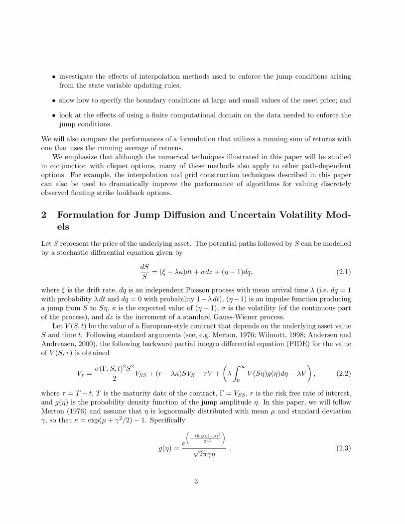
We will construct a deterministic local volatility surface (with no jumps) which is consistentwith the observed market prices (from our synthetic market). We use the expression for the localvolatility surface given by equation (3.14). The exact analytical solution for European optionsunder a Merton jump diffusion model (Merton, 1976) is used to compute the prices and derivativesin equation (3.14). The non-trivial integral in equation (3.14) was computed by converting theintegral to a convolution form and then using an FFT. We could also, of course, use the method inDupire (1994).

Even with an analytical solution, the local volatility becomes unbounded as T → t∗ = 0 forK 6= S∗, and for finite T , with K → 0,∞ (recall Remark 3.3). In particular, the numericalcomputation becomes very ill-posed for T < one month, and for K > 1.5 S∗ and K < .5 S∗ (the

9

Parameter ValueS∗ 100σJ .20r .05λ .10µ -.90γ .45σBS , T = 0.25 .2359σBS , T = 5.0 .3167

Table 1: Parameters for the jump diffusion model, with price process given in equation (3.1). Thejump size distribution is given in equation (2.3). Also shown is σBS, the constant volatility that,if used in a Black-Scholes model with no jumps, reproduces the jump diffusion model price of anat-the-money vanilla call with the specified maturity (T = .25 , 5 ).

initial asset price S∗ = 100). We set a maximum value for the local volatility of 3.0, to avoidproblems with unbounded values from equation (3.14).

We generate a dense grid of σ(S, t) for S ∈ [50, 150], and t ∈ [1/12, 5.0] with S spacing of 1.00and t spacing of 1 month. Any other data needed is obtained by linear interpolation, for values of(S, t) within the grid. For values outside the grid, we use the nearest grid value.

This grid of σ(S, t) values would have to be considered as a very good estimate of the volatilitysurface which matches the synthetic market prices (in practice, we would not have data for farout of the money options with short maturities). The resulting local volatility surface is shown inFigure 1.

Table 2 shows the synthetic market prices of the vanilla calls, at various strikes and times,compared with the prices obtained using the volatility surface shown in Figure 1, computed usingequation (3.14). The fit is quite good, considering that the actual surface which matches all theprices would become unbounded as T → 0, and for K S∗ or K S∗. Recall that we limit themaximum value of σ ≤ 3.0, and we have used a constant surface for t ≤ month.

3.3 Volatility Surface Obtained by Calibration

Of course, in general we would not know the precise representation of the real world process. Amore realistic example of fitting a local volatility surface would be the algorithm in Coleman et al.(1999). To summarize, this method uses a set of specified knot locations, and then attempts todetermine the best L2 fit to the data using a spline interpolant.

Synthetic market prices were generated for vanilla puts and calls at strikes 70, 80, 90, 100, 110, 120, 130,at monthly intervals from [0, 1.0] and yearly intervals from [1.0, 5.0]. These prices were computedusing the exact European prices under a Merton jump diffusion model, with the data in Table 1.In order to avoid unbounded values of the local volatility (i.e. Remark 3.3), as well as improve thefit to the data, the maximum value of the local volatility was constrained to be σ = 1.0.

The knot locations of the spline representation of the local volatility surface were specified to beat S = 70, 100, 130 and at times t = 0.0, 0.5, 1.0, 3.0, 5.0, giving a total of fifteen parameters.Since the number of knot locations for the spline is relatively small, this has the effect of regularizing

10

0.2

0.4

0.6

0.8

1

sigma

01

23

45

Time80100

120

Asset Price

Figure 1: This volatility surface was obtained by using equation (3.14) with the exact analyticalsolution for a European option under a Merton jump diffusion (parameters are given in Table 1).The plot is truncated at a maximum value of σ = 1.0. The actual surface used had a maximumvalue of σ = 3.0.

the surface, as described in Coleman et al. (1999). The resulting volatility surface is shown inFigure 2.

Table 3 shows the error between the prices computed using the surface in Figure 2 and theEuropean call prices. Note that in this case, there is more error for T ≤ 1 and S∗ = 100 comparedto the surface used in Table 2.

4 Cliquet Contracts

4.1 Contract Description

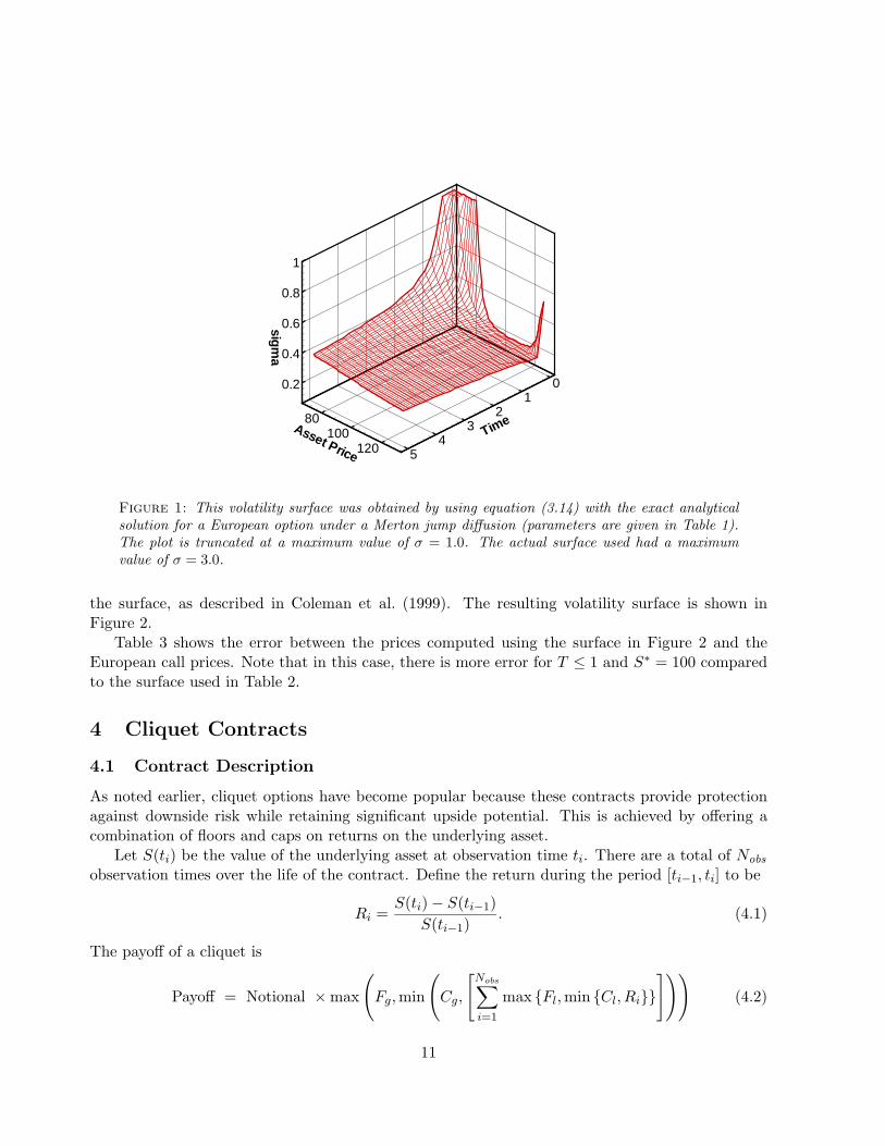
As noted earlier, cliquet options have become popular because these contracts provide protectionagainst downside risk while retaining significant upside potential. This is achieved by offering acombination of floors and caps on returns on the underlying asset.

Let S(ti) be the value of the underlying asset at observation time ti. There are a total of Nobs

observation times over the life of the contract. Define the return during the period [ti−1, ti] to be

Ri =S(ti)− S(ti−1)

S(ti−1). (4.1)

The payoff of a cliquet is

Payoff = Notional ×max

(Fg,min

(Cg,

[Nobs∑i=1

max Fl,min Cl, Ri

]))(4.2)

11

K = 90 K = 100 K = 110Expiry time Vol. Surf. Synthetic Vol. Surf. Synthetic Vol. Surf. Synthetic

1/12 10.67 10.80 2.77 2.75 0.20 0.181/6 11.64 11.71 4.14 4.15 0.79 0.771/4 12.56 12.62 5.30 5.32 1.50 1.491/2 15.18 15.18 8.26 8.27 3.77 3.771 19.69 19.59 13.09 13.07 8.12 8.122 26.83 26.72 20.85 20.78 15.78 15.743 32.67 32.53 27.18 27.07 22.33 22.234 37.64 37.47 32.59 32.43 28.01 27.875 41.99 41.79 37.31 37.12 33.03 32.84

Table 2: Comparison of vanilla call synthetic market prices (jump diffusion model) and the volatil-ity surface model computed using equation (3.14). Input parameters for the jump diffusion modelare given in Table 1. The local volatility surface is shown in Figure 1. The computed prices areaccurate to the number of digits shown.

where Cl, Fl are local caps and floors placed on the individual returns, and Cg, Fg are a global capand floor respectively.

Note that a modification to equation (4.2) is

Payoff = Notional×max

(Fg, R+ min

(0,

[Nobs∑i=1

max Fl,min 0, Ri

]))(4.3)

where R is a specified nominal return. If Fl < 0, then equation (4.3) is the payoff of a reversecliquet. Such contracts give the holder a higher nominal return R in exchange for bearing somedownside market risk.

Since we are solving the PIDE (2.2) backwards in time from the maturity date to the valuationdate, we need to maintain additional state variables as one would in a dynamic programmingcontext. There are two obvious approaches that we now discuss and compare.

4.2 Formulation

4.2.1 Running Sum Formulation

In this case, we introduce two new state variables: P , corresponding to the asset price at theprevious observation, and Z which is defined below. The value of the option is then given byV = V (S, t;P,Z). Assume that tk < t < tk+1. Let

Z(tk < t < tk+1) =k∑i=1

max (Fl,min (Cl, Ri)) , (4.4)

where Z(t < t1) ≡ 0. Consequently, the payoff (4.2) at t = T becomes

Payoff = Notional ×max (Fg,min (Cg, Z)) . (4.5)

12

0.2

0.4

0.6

0.8

1

sigma

01

23

45

Time80100

120

Asset Price

Figure 2: This volatility surface was obtained by using a least squares fit (Coleman et al., 1999)to the exact European call and put prices (under a Merton jump diffusion). The Merton modelparameters are given in Table 1. The actual surface used had a maximum value of σ = 1.0.

Similarly, let P (tk < t < tk+1) = S(tk) denote the value of the asset at the most recent observation.If t−k , t

+k are the times the instant before and after the kth observation, then, following Wilmott

(1998), no-arbitrage considerations lead to the following jump conditions:

R =S − P−

P−

R∗ = max (Fl,min (Cl, R))Z+ = Z− +R∗

P+ = S

V (S, t−;P−, Z−) = V (S, t+;P+, Z+), (4.6)

where P+ = P (t+k ), P− = P (t−k ), Z+ = Z(t+k ), and Z− = Z(t−k ).

4.2.2 Average Formulation

It was demonstrated by Zvan et al. (1999) that the use of the arithmetic average for the additionalstate variable was superior to a running sum formulation in terms of numerical performance forAsian options. Consequently, we will also investigate an alternative formulation which uses average(capped and floored) returns. Again the value of the option is given by V = V (S, t;P,Z) where Pis the previous asset price as defined in the running sum context. However, in this case the state

13

K = 90 K = 100 K = 110Expiry time Vol. Surf. Synthetic Vol. Surf. Synthetic Vol. Surf. Synthetic

1/12 10.81 10.80 3.01 2.75 0.21 0.181/6 11.91 11.71 4.43 4.15 0.82 0.771/4 12.92 12.62 5.60 5.32 1.55 1.491/2 15.49 15.18 8.45 8.27 3.78 3.771 19.69 19.59 13.11 13.07 8.04 8.122 26.82 26.72 20.89 20.78 15.81 15.743 32.64 32.53 27.21 27.07 22.34 22.234 37.57 37.47 32.57 32.43 27.96 27.875 41.91 41.79 37.28 37.12 32.94 32.84

Table 3: Comparison of vanilla call synthetic market prices (jump diffusion model) and the cali-brated volatility surface model (using a low order spline fit (Coleman et al., 1999)). Input parametersfor the jump diffusion model are given in Table 1. The calibrated local volatility surface is shownin Figure 2. The computed prices are accurate to the number of digits shown.

variable Z is defined as

Zavg(tk < t < tk+1) =1k

k∑i=1

max (Fl,min (Cl, Ri)) , (4.7)

where Zavg(t < t1) ≡ 0. In this case payoff (4.2) becomes

Payoff = Notional ×max (Fg,min (Cg, Nobs × Zavg)) . (4.8)

When using the average formulation the jump conditions are given by

R =S − P−

P−

R∗ = max (Fl,min (Cl, R))

Z+avg = Z−avg +

(R∗ − Z−avg)k

P+ = S

V (S, t−;P−, Z−avg) = V (S, t+;P+, Z+avg). (4.9)

An advantage of the average formulation is that the possible range of values of Z = Zavg islimited to min(0, Fl) ≤ Z ≤ Cl, independent of Nobs . In the case of the running sum formulation,the Z values are bounded by min(0, Nobs×Fl) ≤ Z ≤ Nobs×Cl, so that the grid is dependent on thenumber of observations. Notice that we are interested in the solution V (S∗, t = 0;P = S∗, Z = 0),where S∗ is the current value of the underlying asset. As we solve backwards in time, the solutionfor some of the large Z values cannot affect the solution at V (S∗, t = 0;P = S∗, Z = 0) in therunning sum formulation. Consequently, some of the nodes in the Z-direction are wasted unlessthe grid is dynamically reconstructed after each observation.

14

5 Numerical Solution

5.1 Discretization

Note that the PIDE (2.2) is independent of the new state variables (P,Z). Consequently, we candiscretize the state variables as

P1, . . . , Pj , . . . , Pjmax and Z1, . . . , Zk, . . . , Zkmax.

For each discrete value of (Pj , Zk), we can solve the one dimensional PIDE (2.2) at times betweenthe observation dates. To move the solution across an observation date, we use the jump conditions(4.6) or (4.9). Notice that the jump conditions (4.6) and (4.9) are undefined if P = 0. Therefore,it is important to discretize P so that P1 > 0. Note that for geometric Brownian motion withlognormally distributed jumps, a stock price of S = 0 is unattainable in finite time.

For fixed (Pj , Zk), each one-dimensional PDE (2.2) is a function of (S, t) only. Our numericalexperiments utilize Crank-Nicolson timestepping with the modification suggested by Rannacher(1984). Other details of the discretization can be found in Pooley et al. (2003). In particular, weemploy the iterative method described in that paper for the nonlinear uncertain volatility models.In situations where a jump diffusion model was used, the discrete algebraic equations are solvedusing a fixed point iteration combined with an FFT evaluation of the integral term in the PIDE(2.2). This is described in detail in d’Halluin et al. (2005, 2004). The tolerances for all iterativemethods (within each timestep) were set to guarantee that the error in the solution of the discretizedequations did not affect the first six significant digits of the solution.

5.2 Similarity Reduction

As discussed by Forsyth et al. (2002), it is generally necessary to carry out an interpolation operationto approximate the jump conditions at observation dates. Denote the possible dependence of σ onP in equation (2.2) by σ = σ(S, t;P ) (dropping possible dependence on Γ). This interpolation canbe avoided if we assume that

σ(S, t;P ) = σ(ρS, t; ρP ). (5.1)

If equation (5.1) holds, the payoff is given by either (4.5) or (4.8), and the jump conditions aregiven by either (4.6) or (4.9), then from equation (2.2) we have that V is homogeneous of degreezero in (S, P ):

V (S, t;P,Z) = V (ρS, t; ρP,Z) . (5.2)

Setting ρ = P ∗/P gives

V (S, t;P,Z) = V

(S

P× P ∗, t;P ∗, Z

), (5.3)

which implies that we need only solve for one reference value P = P ∗. This effectively reduces thedimensionality of the problem from three to two. As long as the node S = P ∗ is in the S grid,no interpolation is required (in the S direction) to satisfy the jump conditions (4.6) or (4.9). Inthe following, we will refer to assumption (5.1), which then implies equation (5.3), as the similarityreduction.

The assumption (5.1) seems somewhat peculiar, but has a modelling rationale which we willdiscuss in a later section.

15

Asset Price

Pre

viou

sA

sset

Pri

ce

0 100 200 300 400 500 6000

100

200

Figure 3: Repeated grid, constructed using the same asset price S grid for each discrete setting ofthe variable P (the asset price at the preceding observation time).

5.3 Mesh Construction

With regard to the mesh for the Z variable, there are no particularly noteworthy issues. Wesimply use a uniformly spaced grid. However, some issues arise in the construction of the Pgrid (for cases where no similarity reduction is available). Suppose that we use an S grid withSg = S1, . . . , Si, . . . , Simax and a P grid, Pg = P1, . . . , Pj , . . . , Pjmax, with Pg = Sg (i.e. aCartesian product S×P grid, with the same node spacing in the S and P directions). In this case,no interpolation in the S or P directions is required during the application of the state variableupdating rule

P+ = S. (5.4)

A illustration of a set of grids constructed in this fashion is shown in Figure 3. We refer to thisgrid as a repeated grid in the following. We emphasize that a major advantage of a repeated grid,for pricing cliquet options, is that no interpolation error is introduced in the (S, P ) plane at eachobservation date.

In Windcliff et al. (2001), it is shown that this type of grid results in poor convergence for shoutoptions. Normally, we choose a fine node spacing near the initial asset price S = S∗, since this isthe region of most interest. However, since the nodes P = S for all values of S are required duringthe application of the jump condition (5.4), these values may have poor accuracy in areas wherethe S node spacing is large. It is therefore desirable to have a fine node spacing in the S directionfor all nodes near the diagonal of the (S, P ) grid.

Suppose we have a prototype S grid constructed with a fine node spacing near S = S∗. Denotethis set of nodes by Sg = S1, . . . , Si, . . . , Simax. We also assume that the grid has been constructedso that the point S∗ is contained in the discretization. In other words, there is an index i∗ suchthat Si∗ = S∗ and Si∗ ∈ Sg. Let Sjg = Sj1. . . . , S

ji , . . . , S

jimax represent the S nodes corresponding

to the discrete value Pj . The following algorithm is used to construct Sjg , with Pj ∈ Sjg :

16

Asset Price

Pre

viou

sA

sset

Pri

ce

0 100 200 300 400 500 6000

100

200

Figure 4: Scaled grid, constructed using algorithm (5.5).

Scaled Grid Construction

Set Pj = Sj ; j = 1, . . . , imax; Sj ∈ SgSet jmax = imax

For j = 1, . . . , jmax

Sji = SiPj/S∗ i = 1, . . . , imax

EndFor

(5.5)

Since there is an i∗ such that Si∗ = S∗, Sji∗ = Pj . In other words, for each line of constant Pj , thereis a node on the diagonal Sji = Pj , as depicted in Figure 4.

5.4 Interpolation

If Sjg is constructed using algorithm (5.5), then interpolation is required to satisfy the state variableupdating rule (5.4). An obvious method is to linearly interpolate along the S axis and then alongthe P axis, which we refer to as xy interpolation in the following. If we omit the dependence of Von the variables Z and t for brevity, then xy interpolation is defined as:

V (S, P ) = V S(Plow ) +V S(Phigh)− V S(Plow )

Phigh − Plow(P − Plow )

V S(P ) = V (Slow , P ) +V (Shigh , P )− V (Slow , P )

Shigh − Slow(S − Slow )

Slow ≤ S ≤ Shigh

Plow ≤ P ≤ Phigh . (5.6)

In Windcliff et al. (2001) it is argued that diagonal interpolation (along the diagonal of the gridshown in Figure 4) is more suited to capturing the non-smooth payoff of a shout option. Diagonal

17

S

P

70 80 90 100 110 120 13090

100

110

120

Interpolation Point

(a) xy interpolation.

S

P

70 80 90 100 110 120 13090

100

110

120

Interpolation Point

P=S

(b) Diagonal interpolation along P = S.

Figure 5: Different interpolation strategies.

interpolation is defined as

V (S, P = S) = V (S = Plow , Plow ) +V (Phigh , Phigh)− V (Plow , Plow )

Phigh − Plow(S − Plow )

Plow ≤ S ≤ Phigh . (5.7)

Unlike xy interpolation, this method is exact if a similarity reduction is valid. These two approaches(xy and diagonal) are illustrated in Figure 5.

5.5 Boundary Conditions

As previously discussed, away from observation dates, we need to solve a set of one dimensionalPIDEs of the form (2.2) for each discrete value of (P,Z). Consequently, boundary conditions mustbe specified. Normally, a finite computational domain [Smin, Smax] is specified for a one dimensionalBlack-Scholes equation. Usually, Smax is selected to be a large value, and the boundary conditionVSS = 0 is specified at S = Smax as suggested by a variety of authors, including Tavella and Randall(2000) and Wilmott (1998). The reason for this is that many contracts (including cliquets) areasymptotically linear as S →∞. For a discussion of the stability issues surrounding this boundarycondition, see Windcliff et al. (2004). In the following, we will specify VSS = 0 at S = Smax.

Since the PDE degenerates to an ODE at S = 0, which is easily implemented numerically,usually Smin = 0. However, as noted in Section 5.1, the return Ri = (S(ti) − S(ti−1))/S(ti−1)becomes undefined when S(ti−1) = P = 0. Since the jump conditions require that P+ = S, havinga node at S = 0 causes difficulty. Consequently, we should view the solution to the cliquet valuationproblem as being embedded in the computational domain Smin ≤ (S, P ) ≤ Smax, with Smin > 0,and Smax <∞. We seek the solution in the limit as Smin → 0 and Smax →∞. From the nature ofthe cliquet payoff, it is reasonable to impose the boundary condition VSS = 0 at S = Smin as well.Under normal market parameters, setting VSS = 0 at the lower boundary results in a first orderhyperbolic equation with outgoing characteristic, which contrasts with the more delicate situationstudied in Windcliff et al. (2004) at S = Smax. In our numerical tests, we will select a value of Smin

on a coarse grid, and then reduce Smin as the grid is refined, so as to ensure the correct limitingbehavior.

18

5.6 Effect of Finite Computational Domain on the Jump Conditions

If the scaled one dimensional grids are constructed as shown in Figure 4, then there will be situationswhere Sji > Pjmax or Sji < Pjmin . In these cases, our computational domain does not have sufficientdata to allow interpolation of the state variable updating rule P+ = S. If this happens, we assumethat this data can be approximated by assuming that the similarity reduction (5.3) is locally valid.From equation (5.3), this means that

V (Sji , t;P = Sji , Z) ' V (Pjmax , t;Pjmax , Z); Sji > Pjmax

' V (Pjmin , t;Pjmin , Z); Sji < Pjmin . (5.8)

We will refer to (5.8) as a similarity extrapolant. In situations where there is a similarityreduction, this extrapolation scheme is exact. Using a local volatility surface would invalidate theuse of the similarity reduction. However, typically the volatility function is assumed to be constantoutside of some range of asset values near the current asset price. Consider the boundary forlarge asset values. Since the state variable updating rules only query values of S near S = Pjmax ,the effect of far-field errors introduced by the approximation of constant volatility can be madearbitrarily small, as demonstrated by Kangro and Nicolaides (2000).

5.7 Properties of the Discrete Equations

Suppose we solve a full three dimensional cliquet problem, with variables (S, P, Z). Consider thespecial case where a similarity reduction (Section 5.2) is valid. In this case, it seems natural torequire that our grid construction/discretization method is discretely homogeneous of degree zeroin (S, P ), and that there should be no interpolation error incurred in the (S, P ) plane after applyingthe jump conditions. A grid construction/discretization method satisfying these properties shouldalso be useful when solving problems where a similarity reduction is not valid.

Let

Unijk = U(Sji , Pj , Zk, τn) (5.9)

be the discrete solution to the cliquet pricing problem. Note that we have allowed the grid Sjg todepend on Pj . Let Unjk be the vector of discrete solution values for grid Sjg , i.e.

(Unjk)i = Unijk . (5.10)

Since equation (2.2) contains no derivatives w.r.t. (P,Z), then, given Unij , we can solve for Un+1ij

for each (jk) independently. If a fully implicit (θ = 1) or Crank-Nicolson (θ = 1/2) timesteppingmethod is used, and equation (2.2) is discretized as in d’Halluin et al. (2005, 2004), then we havethat

(I + θMj)Un+1jk = (I − (1− θ)Mj)Unjk , (5.11)

where Mj = M(Sji , Pj) is the matrix form of the discretization operator (for a given grid Sjg).Note that since equation (2.2) is independent of Z, then Mj has no k dependence.

We first gather some conditions which are required for a similarity reduction (Section 5.2) tobe valid.

19

Conditions 5.1 (Conditions for a Similarity Reduction) The following conditions are requiredin order to use the similarity reduction method described in Section 5.2.

• The payoff of the cliquet is homogeneous of degree zero in (S, P ), i.e. for any scalar λ > 0

V (λS, λP, Z, τ = 0) = V (S, P, Z, τ = 0) . (5.12)

• The discrete form of the PIDE operator (2.2) is homogeneous of degree zero in (S, P ), i.e.for any scalar λ > 0

M(λSji , λPj) = M(Sji , Pj) (5.13)

• The jump conditions are given as in (4.6) and (4.9).

Remark 5.1 (Homogeneity Property of the Discrete Operator) Property (5.13) holds if ei-ther σ = const. in equation (2.2), or σ satisfies condition (5.1); and, in addition, boundary con-ditions VSS = 0 are imposed at S = Smin, Smax, and the discretization method in d’Halluin et al.(2005, 2004) is used.

We also gather some conditions on the grid construction, discretization and jump conditionenforcement that we wish to impose.

Conditions 5.2 (Grid Construction/Discretization Properties) We assume that the grid isconstructed with the following conditions

• The mesh is constructed using the scaled grids as described in Algorithm 5.5.

• Diagonal interpolation (5.7) is used where required to enforce the jump conditions. The sim-ilarity extrapolant (5.8) is used if missing data is required.

• The boundary condition VSS = 0 is imposed for each grid at S = Sjmin, S = Sjmax.

We can now state an interesting property of grid construction and discretization methods whichsatisfy Conditions 5.2.

Property 5.1 (Grid Construction/Discretization Property) Provided that the similarity re-duction Conditions 5.1 are satisfied, and the grid is constructed satisfying Conditions 5.2 then

Unijk = Unij∗k ; ∀i, j, k, n , (5.14)

where j∗ denotes the index such that Pj∗ = S∗. Equation (5.14) then implies that

U(λSji , λPj , Zk, τn) = U(Sji , Pj , Zk, τ

n)

λ =PlPj

, (5.15)

which can be interpreted as a discrete homogeneity property. In addition, there is no interpolationerror introduced in the (S, P ) planes upon applying jump conditions (4.6) or (4.9).

20

Proof . Suppose that the scaled grid for Sji is constructed as in Algorithm 5.5. Since the payoffis homogeneous of degree zero in (S, P ) (condition (5.12)), then at timestep n = 0, we have

U0ijk = U(Sji , Pj , Zk, τ = 0)

= U(PjS∗Si,

PjS∗

S∗, Zk, τ = 0)

= U(Si, S∗, Zk, τ = 0)= U0

ij∗k , (5.16)

Suppose that at timestep n, we have that

Unijk = Unij∗k . (5.17)

From condition (5.13) we have that

Mj = M

(PjS∗Si

,PjS

∗

S∗

)= M(Si, S∗)= Mj∗ , (5.18)

It then follows from equation (5.11), using equations (5.17) and (5.18) that

Un+1jk = (I + θMj)−1(I − (1− θ)Mj)Unjk

= (I + θMj∗)−1(I − (1− θ)Mj∗)Unj∗k= Un+1

j∗k . (5.19)

Consequently, since U0jk = U0

j∗k, then Unjk = Unj∗k for all steps between applications of the jumpconditions.

Let (Un+1jk )− = (Un+1

j∗k )− be the discrete solution the instant before application of the jumpconditions (going backwards in time), and (Un+1

jk )+ be the solution the instant after application ofthe jump conditions (backwards in time). If the jump conditions (4.6) or (4.9) are specified, and ifdiagonal interpolation (5.7) is used, along with the similarity extrapolant (5.8), then it is easy tosee that

(Un+1jk )+ = (Un+1

j∗k )+ , (5.20)

hence properties (5.14) and (5.15) hold after application of the jump conditions. Note that thejump conditions (4.6) or (4.9) require evaluation of (noting equation (5.15))

(U(Sji , Sji , Z, τ

n+1)− = (U(S∗, S∗, Z, τn+1)− (5.21)

hence from equation (5.7), there is no interpolation error in the (S, P ) plane with diagonal inter-polation.

21

Remark 5.2 (Significance of Property 5.1) If the Conditions 5.1 for a similarity reductionare rigorously satisfied, and the grid is constructed satisfying Conditions 5.2, then the solutionvector is discretely homogeneous of degree zero in (S, P ), as in equation (5.15). Furthermore,application of the jump conditions does not generate any interpolation error in the (S, P ) plane.In this case, we need only solve for a single value of P = S∗ in each (S, P ) plane, i.e. there is noneed to solve a full three dimensional problem. However, in cases where the similarity reductionis not valid, we expect that a grid satisfying Conditions 5.2 will still be desirable. For example,if σ = σ(S, t), then in general a similarity reduction cannot be used. However, any interpolationerror introduced by the diagonal interpolant (on the grid satisfying Conditions 5.2) will be a result ofdeviations from a constant volatility, which we expect to be small in regions where the local volatilityfunction is smooth.

6 Numerical Tests: Methods

6.1 Comparison of Running Sum and Average Formulations

As a first test we compare the convergence of the running sum and average formulations as thegrid size is refined and number of timesteps is increased. Details of the contract used in these testsare provided in Table 4. Note that the contract is the same as that studied in Wilmott (2002).For these tests we use a constant volatility model without jumps. Input parameters are presentedTable 5.

The results of the convergence tests are shown in Table 6. Since σJ = const., we can use thesimilarity reduction to reduce this to a two dimensional PDE. A series of tests was carried outwhere at each refinement level new nodes were inserted between each pair of nodes in the coarsergrid, a new node was added between 0 and Smin from the previous grid, and the timestep size wasreduced by a factor of two. Contrary to the results found by Zvan et al. (1999) for Asian options,the running sum formulation seems to be converging faster than the average formulation. In allsubsequent tests, we will use the running sum formulation.

Note that we use second order methods to discretize each one dimensional PIDE as described ind’Halluin et al. (2005, 2004). The jump conditions are also imposed using linear interpolation in theZ direction, which would also have quadratic error for smooth solutions (assuming a finite numberof observations). However, application of the jump conditions (4.9) results in a non-smoothness

Parameter ValueObservation times 1.0, 2.0, 3.0, 4.0, 5.0T 5.0Notional 1.0Cl 0.08Fl 0.0Cg ∞Fg 0.16

Table 4: Cliquet contract details.

22

Parameter ValueS∗ 100σJ 0.20r 0.03λ 0.0

Table 5: Parameters for the constant volatility case without jumps.

Nodes Timesteps Value Change RatioRunning Sum Formulation

31× 13 40 0.17446731262× 25 80 0.174230223 .00023709124× 49 160 0.174099404 .00013082 1.8248× 97 320 0.174066778 .00003262 4.0496× 193 640 0.174060717 .00000606 5.4

Average Formulation31× 13 40 0.17480739062× 25 80 0.174368430 .00043896124× 49 160 0.174207223 .00016121 2.7248× 97 320 0.174110595 .00009663 1.7496× 193 640 0.174089486 .00002111 4.6

Table 6: Value of a cliquet option using the running sum and average formulations. Contractdetails are provided in Table 4. Parameters are given in Table 5. Nodes refers to the number ofnodes in the S and Z directions respectively. A similarity reduction is used, so no grid is needed inthe P direction. At each refinement level, new nodes are inserted between each pair of grid nodeson the coarser grid, a new node is added between S = 0 and the first coarser grid node, and thetimestep size is halved. Change refers to the change in numerical value from one level of refinementto the next. Ratio refers to the ratio of changes between successive refinements. An asymptoticratio of four indicates quadratic convergence.

of the solution in the Z direction, due to the local caps and floors. This non-smoothness can beexpected to cause the convergence rate to be somewhat erratic. We can see in Table 6 that theratio of changes departs somewhat from the ideal asymptotic value of four which would be observedfor exact quadratic convergence.

6.2 Effect of Grid and Interpolation

Using the local volatility surface shown in Figure 1, obtained using equation (3.14), and the contractoutlined in Table 4, a series of convergence tests was carried out. These are shown in Table 7. Inthis case no similarity reduction is possible since the volatility surface is a general function of Sand t and does not satisfy equation (5.1). As before, a series of refined grids was constructed whereon each refinement the timestep size was halved, new nodes were inserted between each coarse gridnode, and a new node was inserted in the S grid in (0, Smin).

The results in Table 7 indicate that using a Cartesian product grid (Repeated Grid) that uses

23

the same node spacing in the (S, P ) directions results in very poor convergence even though thereis no interpolation error in the (S, P ) directions when applying the jump conditions. Clearly, theuse of the scaled grid/discretization method satisfying Conditions 5.2 is very effective. Hence, wewill use these methods in the following.

Nodes Timesteps Scaled Grids Scaled Grids Repeated(diagonal interpolation) (xy interpolation) Grid

35× 35× 13 40 .167847 .169728 .14823070× 70× 25 80 .167229 .167837 .159672

140× 140× 49 160 .167046 .167211 .164720

Table 7: Value of a cliquet option with a volatility surface (Figure 1 and equation (3.14)). Contractdetails are provided in Table 4. Nodes refers to the number of nodes in the S, P , and Z directionsrespectively. Scaled grids refers to the S-grid construction method (5.5), shown in Figure 4, andsatisfying Conditions 5.2. Diagonal interpolation refers to interpolation method (5.7), shown inFigure 5(b), whereas xy interpolation refers to the interpolation method (5.6), shown in Figure 5(a).Repeated grid refers to a Cartesian product grid with the same node spacing in the S and P directions(Figure 3).

6.3 Effect of Boundary at S = Smax

Table 8 shows the effect of choosing different values of Smax. The results were obtained using thevolatility surface in Figure 1, with grids/discretization satisfying Conditions 5.2. The initial coarsegrid with 35× 35× 13 nodes used Sjmax = 18× Pj . The initial grid with 31× 31× 13 nodes usedSjmax = 4 × Pj . As we can see, there is no effect on the solution (to six figures) of imposing theboundary condition VSS = 0 at these values of Smax. Note that this is because we use both scaledgrids (as shown in Figure 4), and the similarity extrapolant (5.8) where necessary to impose jumpconditions. In the following, we use Sjmax = 18× Pj .

Nodes Timesteps Scaled Grids Nodes Timesteps Scaled Grids35× 35× 13 40 .167847 31× 31× 13 40 .16784770× 70× 25 80 .167229 62× 62× 25 40 .167229

140× 140× 49 160 .167046 124× 124× 25 160 .167046

Table 8: Value of a cliquet option with a volatility surface (Figure 1 and equation (3.14)). Con-tract details are provided in Table 4. Nodes refers to the number of nodes in the S, P , and Zdirections respectively. Scaled grids refers to the S-grid construction method (5.5), shown in Fig-ure 4. Diagonal interpolation refers to interpolation method (5.7), shown in Figure 5(b). The basegrid 35× 35× 13 used Sjmax = 18× Pj. The reduced base grid 31× 31× 13 used Sjmax = 4× Pj.

24

7 Numerical Tests: Modelling Assumptions

7.1 Volatility Surface Based on Analytic Expression

There is increasing evidence that jump processes provide reasonable explanations of volatility smilesand skews. If the real stock price process is a jump diffusion, then the common approach of fittinga volatility surface to vanilla option prices can, as we will demonstrate, result in a significant errorwhen pricing exotic options such as cliquet contracts. However, as we shall see, it is standardpractice in industry to use various methods to correct for these deficiencies. These corrections doappear to reduce the pricing errors dramatically, but only near S = S∗, the initial asset price.

We assume that the synthetic market dynamics are given by the parameters in Table 1 andthe contract details are contained in Table 4. We use the local volatility surface constructed usingequation (3.14), as described in Section 3.2. The surface is shown in Figure 1.

The resulting value of a cliquet option is given in Table 9. At each refinement level, new nodesare inserted between each two coarse grid nodes, and the timestep is halved. As we increase therefinement level, the solution will converge to the correct value. The column “Vol. Surf.” of thistable provides corresponding results if we value this same option without using a jump diffusionmodel but instead using a volatility surface which was fit to our synthetic vanilla market data(arising from a jump model). Note that these are quite different from the correct values, at leastin our synthetic market. This is also illustrated in Figure 6.

Refinement Jump Diffusion Vol. Surf. Vol. Surf. Vol. Surf. Const. Vol. Const. Vol.Level Const. Vol. (Fig 1) Sim. Red. Sim. Red. σ = .2359 σ = .3167

Rebased t

0 .177303 .167847 .170017 .178142 .163874 .1602531 .177515 .167229 .169491 .177942 .163415 .1595332 .177540 .167046 .169358 .177909 .163259 .159339

Table 9: Value of a cliquet option under jump diffusion with constant volatility (parameters aregiven in Table 1) and various other volatility models. The volatility surface is computed using themethod described in Section 3.2, using equation (3.14), ans shown in Figure 1. Contract detailsare provided in Table 4. Volatility surface shown in Figure 1, computed using equation (3.14).Vol. Surf. refers to a volatility surface model with no jumps. Vol. Surf. Sim. Red. refers to theassumption of equation (5.1), and no jumps. Vol. Surf. Sim. Red. Rebased t refers to assumption(7.5), and no jumps. Const. Vol. models have no jumps (values of σ are provided in Table 1). Ateach refinement level, new nodes are inserted between each coarse grid node, and the timestep ishalved.

Figure 6 compares the true synthetic market price (t∗ = 0) compared with the local volatilityapproach. This Figure shows the value of V (S, P = S∗, Z = 0, t = 0). Note that the minimumvalue of this contract, independent of the underlying model and initial asset price, is about .1246,so that the error, relative to this minimum value, is quite large near the current price S∗ = 100.

However, practitioners are well aware of the problems with using a calibrated local volatilitysurface to price exotics. If we calibrate a local volatility surface at t = t∗ with S∗ = P , andsubsequently assume that equation (5.1) holds, then a modelling decision has been made to assumethat the volatility surface is a function of S/P . We can think of this as assuming that the observed

25

Asset Price

Opt

ion

Val

ue

50 75 100 125 150

0.125

0.15

0.175

0.2 Jump Diffusion

VolatilitySurface

Minimum Value

Figure 6: Cliquet option value. Comparison of jump diffusion model with constant volatility(parameters are given in Table 1) with a volatility surface (Figure 1). The surface is computedusing the method described in Section 3.2.

volatility skew will always be “centered” in some sense around the current asset level. This can bejustified on the basis of Lemma 3.2 in Section 3. If we calibrate a local volatility model (assumingprocess (3.3)) to prices generated where the process actually follows (3.1), then in the case ofσJ = const., Lemma 3.2 states

σL(ρS∗, t∗; ρS, t) = σL(S∗, t∗;S, t), (7.1)

where σL is the local volatility, determined by calibration as described in Section 3. If we let S∗ = Pin equation (7.1), then

σL(ρP, t∗; ρS, t) = σL(P, t∗;S, t)

= σL

(S∗, t∗;

S

P× S∗, t

). (7.2)

Therefore, if σ(S, t;P ) = σL(P, t∗;S, t), then equation (5.1) holds.Another common assumption made by practitioners is to rebase the time for the evaluation

of the volatility surface in order to fix the forward starting volatility skew dynamics. To explain,if we calibrate the surface initially at time t∗, then we will typically observe a heavy skew in theimplied volatilities of short dated options maturing near t∗. For longer dated options, expiring atti t∗, the volatility surface is much flatter. When hedging cliquet positions, we may want to takestatic positions in market traded options at observation dates in order to reduce model risk. If were-calibrate the volatility surface at time ti, usually we will find that the new surface now has aheavy skew for options maturing close to ti, which are now short dated options. If tk−1 ≤ t ≤ tk,where tk are observation dates, then it can be postulated that

σ(S, t;P ) = σL(P, tk−1;S, t− tk−1). (7.3)

26

In our case since σJ = const., then

σL(P, tk−1;S, t− tk−1) = σL(P, t∗;S, t− tk−1). (7.4)

Combining assumptions (5.1), (7.1), and (7.4) together gives

σ(S, t;P ) = σ(ρS, t; ρP )= σL(ρP, t∗; ρS, t− tk−1)

= σL

(S∗, t∗;

S

P× S∗, t− tk−1

)(7.5)

where σL is the volatility surface calibrated to prices at tk−1, and we have assumed that thecalibration is carried out at stock price S∗ = P at time tk−1. Again, these modelling assumptionsare often used by practitioners to mitigate the skew of the volatility surface and its flattening out,as one looks farther ahead in time.

Values for the cliquet option under assumption (7.1) or (7.5) are also given in Table 9 (columnsheaded “Vol. Surf. Sim. Red.” and “Vol. Surf. Sim. Red. Rebased t”). In the latter case, theagreement between the volatility surface and the true synthetic market price is excellent. Note thateither of the assumptions (7.1) or (7.5) allow us to use the similarity reduction method describedin Section 5.2.

Finally, we also value this cliquet contract using constant volatility models (no jumps). Theresulting values are poor approximations (see Table 9). The volatility values are obtained bycalibration to a single at-the-money call (priced in our synthetic jump diffusion market) at twodifferent maturities.

Although Table 9 suggests that the common practitioner adjustments to compensate for thedeficiencies of a calibrated local volatility surface perform very well, this is a bit misleading. Figure7 gives a plot of a comparison of the synthetic market price, and the prices which result fromthe local volatility with the additional assumptions (7.1) and (7.5). We can see that, under thesimilarity reduction, rebased time approximation (assumption (7.5)), the price agreement is onlygood near S = S∗, and deviates substantially as we move away from S∗ = 100.

This problem can be seen more clearly by plotting the option delta. Figure 8 shows the optiondelta for the case of the jump diffusion model and the volatility surface model constructed usingequation (3.14), and shown in Figure 1. We use the similarity reduction and rebased time assump-tion (7.5). Even though the values for the cliquet option are comparable close to S∗ = 100 (seeFigure 7), the deltas are significantly different.3

7.2 Volatility Surface Obtained by Calibration

In Table 10, we show the cliquet prices computed using the surface in Figure 2. We remind thereader that this surface was computed using the method in Section 3.3, which calibrates to vanillaprices using a least squares fit to a spline representation of the surface (Coleman et al., 1999).

Once again we see that the fitted local volatility surface cliquet prices are considerably in error,compared to the exact synthetic market price. However, the use of the rebased time and forced

3Note that in the context of a jump diffusion model, the hedging portfolio should include additional options tominimize the jump risk (Andersen and Andreasen, 2000).

27

Asset Price

Opt

ion

Val

ue

50 75 100 125 150

0.125

0.15

0.175

0.2 Jump Diffusion

Volatility SurfaceSimilarity Reduction

Asset PriceO

ptio

nV

alue

50 75 100 125 150

0.125

0.15

0.175

0.2

Jump Diffusion

Volatility SurfaceSimilarity ReductionRebasedTime

Figure 7: Cliquet option value. Comparison of the jump diffusion model with constant volatility(parameters are given in Table 1) and the volatility surface approximation. Left panel: volatilitysurface with a similarity reduction (equations (7.1). Right panel: volatility surface with a similarityreduction, rebased time (equations (7.1) and (7.5)). The volatility surface is computed using themethod described in Section 3.2, using equation (3.14). The surface is shown in Figure 1.

Asset Price

Del

ta

50 75 100 125 1500

0.0002

0.0004

0.0006

0.0008

0.001

Jump Diffusion

Volatility SurfaceSimilarity ReductionRebased Time

Figure 8: Cliquet option delta. Comparison of jump diffusion model with constant volatility(parameters are given in Table 1) with a calibrated volatility surface with a similarity reduction(equations (7.1) and (7.5)). The volatility surface is computed with the method described in Section3.2, and using equation (3.14). The surface is shown in Figure 1.

28

homogenization of the volatility surface (as in equation (7.5)) considerably reduces the error. Theerror is, naturally, not as small as is obtained using the expression (3.14), as shown in Table 9.

Refinement Jump Diffusion Vol. Surf. Vol. Surf. Vol. Surf.Level Const. Vol. (Fig 2) Sim. Red. Sim. Red.

Rebased t

0 .177303 .169180 .172563 .1812261 .177515 .168433 .171966 .1808022 .177540 .168193 .171866 .180569

Table 10: Value of a cliquet option under jump diffusion with constant volatility (parameters aregiven in Table 1) and various other volatility models. The volatility surface was computed using aspline fit to the European prices (Coleman et al., 1999), as described in Section 3.3. The surfaceis shown in Figure 2. Contract details are provided in Table 4. Vol. Surf. refers to a volatilitysurface model with no jumps. Vol. Surf. Sim. Red. refers to the assumption of equation (5.1), andno jumps. Vol. Surf. Sim. Red. Rebased t refers to assumption (7.5), and no jumps. Const. Vol.models have no jumps (values of σ are provided in Table 1). At each refinement level, new nodesare inserted between each coarse grid node, and the timestep is halved. Compare with Table 9.

Figure 9 verifies that the use of the calibrated local volatility model (Figure 2), with the ad-ditional assumptions (7.1) and (7.5), yields good agreement with the synthetic market price nearS = S∗, but poor agreement elsewhere.

7.3 Uncertain Volatility

As pointed out by Wilmott (2002), valuing cliquets with extreme values of constant volatility doesnot really capture the risk of mis-specification of volatility. Wilmott suggests using an uncertainvolatility model to quantify the effect of volatility risk. Table 11 provides the best-worst case pricesof a cliquet option in an uncertain volatility model, where σmin and σmax are taken from Table 1.Table 11 reveals a large spread between the two cases.

Refinement Worst Case Best CaseLevel Long Long

0 .150548 .1756571 .149929 .1751832 .149745 .175049

Table 11: Value of a cliquet option using an uncertain volatility model (no jumps) with r = .05 ,σmin = .2359 , and σmax = .3167 . Contract details are provided in Table 4.

Figure 10(a) shows the jump diffusion price and the best-worst case uncertain volatility prices.Surprisingly, the uncertain volatility best case value is quite close to the jump diffusion value, butwe suspect that this is will not be true in general. Note that the best case price is not always abovethe jump diffusion price. This is because the best case price is guaranteed to be above the constantvolatility price only for pure diffusion models. This is illustrated in Figure 10(b).

29

Asset Price

Opt

ion

Val

ue

50 75 100 125 150

0.125

0.15

0.175

0.2 Jump Diffusion

VolatilitySurface

Asset PriceO

ptio

nV

alue

50 75 100 125 150

0.125

0.15

0.175

0.2

Jump Diffusion

Volatility SurfaceSimilarity ReductionRebasedTime

Figure 9: Cliquet option value. Comparison of jump diffusion model with constant volatility(parameters are given in Table 1). The volatility surface is computed using the spline fit proceduredescribed in Coleman et al. (1999). Left panel: pure volatility surface. Right panel: volatility surfacewith a similarity reduction, rebased time (equations (7.1) and (7.5)). Compare with Figure 7. Notethat the local volatility in this case was obtained using the method in Section 3.3, and the surfaceis given in Figure 2.

Asset Price

Opt

ion

Val

ue

50 75 100 125 150

0.125

0.15

0.175

0.2Jump Diffusion

Uncertain VolatilityBest Case

Uncertain VolatilityWorst Case

(a) Cliquet option value. Comparison ofjump diffusion model (constant volatility,parameters in Table 1) with an uncertainvolatility model, σmin = .2359 , σmax =.3167 .

Asset Price

Opt

ion

Val

ue

50 75 100 125 150

0.125

0.15

0.175

0.2

Uncertain VolatilityBest Case

Uncertain VolatilityWorst Case

σ = .2369

σ = .3167

(b) Cliquet option value. Comparisonof constant volatility model (no jumps)with an uncertain volatility model, σmin =.2359 , σmax = .3167 .

Figure 10: Uncertain volatility examples.

30

Asset Price

Opt

ion

Val

ue

50 75 100 125 1500.15

0.16

0.17

0.18

0.19

0.2

0.21

0.22

0.23

0.24

0.25

0.26

0.27

Jump Diffusion

Volatility SurfaceSimilarity ReductionRebasedTime

(a) Volatility surface computed usingequation (3.14) as shown in Figure 1.

Asset PriceO

ptio

nV

alue

50 75 100 125 1500.15

0.16

0.17

0.18

0.19

0.2

0.21

0.22

0.23

0.24

0.25

0.26

0.27

Jump Diffusion

Volatility SurfaceSimilarity ReductionRebasedTime

(b) Volatility surface computed using themethod in Coleman et al. (1999), as shownin Figure 2.

Figure 11: Reverse cliquet option value (S∗ = 100 , t = 0 ). Comparison of jump diffusionmodel with constant volatility (parameters are given in Table 1), with a volatility surface, similarityreduction model, rebased time, as in equation (7.5). Contract details are provided in Table 12.

7.4 Reverse Cliquet Example

As a final example, we consider a reverse cliquet, with the payoff given in equation (4.3). Thecontract details are given in Table 12.

Parameter ValueS∗ 100Observation times 1.0, 2.0, 3.0, 4.0, 5.0T 5.0Notional 1R .50Fl -.15Fg .10

Table 12: Reverse cliquet contract details.

Figure 11 compares the jump diffusion results for the reverse cliquet, and the volatility surfacesshown in Figure 1 and Figure 2, with the similarity reduction and rebased time modifications (7.5).As with the regular cliquet, there is good agreement between the synthetic market price and thelocal volatility model, as long as S ∼ S∗. However, there are significant differences in the shapeof the two curves. This indicates that the deltas computed with the volatility surface will be quitedifferent from the deltas computed with the jump diffusion model.

31

8 Conclusions

Recent turmoil in financial markets has heightened investor awareness of the effect of volatilityon portfolios. Cliquet options have become popular insurance against market volatility for largepension plans as well as retail investors. It is therefore of interest to have effective techniques forvaluing and hedging these instruments.

The discretely observed cliquet valuation problem reduces to solving a set of one dimensionalPDEs embedded in a two or three dimensional space. These one dimensional problems exchangeinformation through jump conditions at each sampling date. With respect to numerical issues, ourmain results are:

• Unlike the case for discretely observed Asian options, the running sum formulation seemssuperior to the running average return formulation.

• The type of grid used and interpolation method employed for enforcement of the jump con-ditions at observation dates has a very large impact on the convergence of the solution. Inparticular, we recommend using a special scaling method for constructing each one dimen-sional grid, coupled with diagonal interpolation, and an extrapolation method for determiningmissing data at the extremes of the grid.

From a practical point of view, we also observe that cliquet options are sensitive to the volatilitymodel assumed. If constant volatilities are used, the value of the cliquet option is insensitive to anextreme range of volatilities. On the other hand, if an uncertain volatility model is used, there isa large spread between best and worst case values.

Recently, jump diffusion models have been touted as better models of market dynamics thanthe commonly used volatility surface model. If we assume a synthetic market which is driven by ajump diffusion process, and then calibrate a volatility surface model (no jumps) to vanilla optionprices generated in the synthetic market, there is a large discrepancy between the value obtainedfor a cliquet option using the calibrated volatility surface compared to the true value found usingthe jump diffusion model.

The limitations of volatility surfaces for modelling forward start type options are well known.Practitioners attempt to correct for these problems by

• forcing the local volatility function to homogeneous of degree zero in current price and priceat last reset; and

• rolling the local volatility surface forward, i.e. using only the small time part of the surface,to avoid the flattening of the skew.

If the usual local volatility is modified by these two corrections, the price of the cliquet at theinitial asset price is in very close agreement with the synthetic market price. However, if we moveaway from the initial asset price, the agreement deteriorates. The deltas from the corrected localvolatility approach are quite different from the synthetic market deltas.

This result suggests that use of calibrated volatility surface models for cliquet options shouldbe viewed with suspicion. If the corrected local volatility function is used, the prices are reasonablyaccurate, but only at a single point. An uncertain volatility model, as suggested in Wilmott (2002),

32

which generates a large spread between best and worst cases, at least signals to the hedger the realvolatility risk involved in writing these options.

References

Andersen, L. and J. Andreasen (2000). Jump-diffusion processes: Volatility smile fitting andnumerical methods for option pricing. Review of Derivatives Research 4, 231–262.

Avellaneda, M., A. Levy, and A. Paras (1995). Pricing and hedging derivative securities in marketswith uncertain volatilities. Applied Mathematical Finance 2, 73–88.

Coleman, T. F., Y. Li, and A. Verma (1999). Reconstructing the unknown local volatility function.Journal of Computational Finance 2, 77–102.

Cont, R. and P. Tankov (2004). Financial Modelling with Jump Processes. Chapman & Hall/CRC.

d’Halluin, Y., P. Forsyth, and G. Labahn (2004). A penalty method for American options withjump diffusion processes. Numerische Mathematik 97, 321–352.

d’Halluin, Y., P. A. Forsyth, and K. R. Vetzal (2005). Robust numerical methods for contingentclaims under jump diffusion processes. IMA Journal of Numerical Analysis 25, 87–112.

Dupire, B. (1994). Pricing with a smile. Risk 7 (January), 18–20.

Forsyth, P. A. and K. R. Vetzal (2001). Implicit solution of uncertain volatility/transaction costoption pricing models with discretely observed barriers. Applied Numerical Mathematics 36,427–445.

Forsyth, P. A., K. R. Vetzal, and R. Zvan (2002). Convergence of lattice and PDE methods forvaluing path dependent options using interpolation. Review of Derivatives Research 5, 273–314.

Garroni, M. G. and J. L. Menaldi (1992). Green Functions for Second Order Parabolic Integro-differential Problems. Number 275 in Pitman Research Notes in Mathematics. Longman Scientificand Technical, Harlow, Essex, UK.

Hirsa, A., G. Courtadon, and D. B. Madan (2003). The effect of model risk on the valuation ofbarrier options. The Journal of Risk Finance 4, 47–55.

Kangro, R. and R. Nicolaides (2000). Far field boundary conditions for Black-Scholes equations.SIAM Journal on Numerical Analysis 38, 1357–1368.

Lyons, T. (1995). Uncertain volatility and the risk free synthesis of derivatives. Applied Mathemat-ical Finance 2, 117–133.

Merton, R. C. (1973). Theory of rational option pricing. Bell Journal of Economics and Manage-ment Science 4, 141–183.

Merton, R. C. (1976). Option pricing when underlying stock returns are discontinuous. Journal ofFinancial Economics 3, 125–144.

33

Pooley, D. M., P. A. Forsyth, and K. R. Vetzal (2003). Numerical convergence properties of optionpricing PDEs with uncertain volatility. IMA Journal of Numerical Analysis 23, 241–267.

Rannacher, R. (1984). Finite element solution of diffusion problems with irregular data. NumerischeMathematik 43, 309–327.

Roach, G. E. (1982). Green’s Functions. Cambridge University Press.

Schoutens, W., E. Simons, and J. Tistaert (2004). A perfect calibration: Now what? WilmottMagazine March, 66–78.

Tavella, D. and C. Randall (2000). Pricing Financial Instruments: The Finite Difference Method.Wiley.

Vetzal, K. R. and P. A. Forsyth (1999). Discrete Parisian and delayed barrier options: A generalnumerical approach. Advances in Futures and Options Research 10, 1–16.

Walliser, J. (2003). Retirement guarantees in mandatory defined contribution systems. In O. S.Mitchell and K. Smetters (Eds.), The Pension Challenge: Risk Transfers and Retirement IncomeSecurity, Chapter 11, pp. 238–250. Oxford University Press.

Wilmott, P. (1998). Derivatives: The Theory and Practice of Financial Engineering. Wiley.

Wilmott, P. (2002). Cliquet options and volatility models. Wilmott Magazine December, 78–83.

Windcliff, H., P. A. Forsyth, and K. R. Vetzal. Pricing methods and hedging strategies for volatilityderivatives. Journal of Banking and Finance, forthcoming.

Windcliff, H., P. A. Forsyth, and K. R. Vetzal (2001). Shout options: A framework for pricingcontracts which can be modified by the investor. Journal of Computational and Applied Mathe-matics 134, 213–241.

Windcliff, H., P. A. Forsyth, and K. R. Vetzal (2004). Analysis of the stability of the linear boundarycondition for the Black-Scholes equation. Journal of Computational Finance 8 (Fall), 65–92.

Zvan, R., P. A. Forsyth, and K. R. Vetzal (1999). Discrete Asian barrier options. Journal ofComputational Finance 3 (Fall), 41–67.

34