numerical method for darcy flow derived using discrete exterior calculus

NUMERICAL METHOD FOR DARCY FLOWDERIVED USING DISCRETE EXTERIOR CALCULUS

ANIL N. HIRANI, KALYANA B. NAKSHATRALA, AND JEHANZEB H. CHAUDHRY

Abstract. We derive a numerical method for Darcy flow, hence also forPoisson’s equation in first order form, based on discrete exterior calculus(DEC). Exterior calculus is a generalization of vector calculus to smoothmanifolds and DEC is its discretization on simplicial complexes such astriangle and tetrahedral meshes. We start by rewriting the governingequations of Darcy flow using the language of exterior calculus. Thisyields a formulation in terms of flux differential form and pressure. Thenumerical method is then derived by using the framework provided byDEC for discretizing differential forms and operators that act on forms.We also develop a discretization for spatially dependent Hodge star thatvaries with the permeability of the medium. This also allows us toaddress discontinuous permeability. The matrix representation for ourdiscrete non-homogeneous Hodge star is diagonal, with positive diagonalentries. The resulting linear system of equations for flux and pressureare saddle type, with a diagonal matrix as the top left block. Ourmethod requires the use of meshes in which each simplex contains itscircumcenter. The performance of the proposed numerical method isillustrated on many standard test problems. These include patch tests intwo and three dimensions, comparison with analytically known solutionin two dimensions, layered medium with alternating permeability values,and a test with a change in permeability along the flow direction. Ashort introduction to the relevant parts of smooth and discrete exteriorcalculus is included in this paper. We also include a discussion of theboundary condition in terms of exterior calculus.

1. Introduction

We have discretized the equations of Darcy flow and obtained a numer-ical method on staggered mesh pairs with fluxes and pressures being theprimary variables. The numerical method was obtained by using discreteexterior calculus (DEC) [22, 23, 28]. Exterior calculus generalizes vectorcalculus to higher dimensions and to smooth manifolds [1] and DEC is itsdiscretization. This discretization yields numerical methods for solving par-tial differential equations (PDEs) on simplicial complexes, such as triangle,

Date: October 18, 2008, Version 1.5264.2000 Mathematics Subject Classification. Primary 65N30, 76S05; Secondary 53-04, 55-

04.Key words and phrases. discrete exterior calculus; mixed method; finite element

method; finite volume method; Darcy flow; Poisson’s equation.

1

2 A. N. HIRANI, K. B. NAKSHATRALA, AND J. H. CHAUDHRY

tetrahedral or higher dimensional simplicial meshes. A recent implemen-tation of DEC is described in [7]. DEC is related to many discretizationsof exterior calculus that have been popular in or are currently being pur-sued in numerical analysis. Others include finite element exterior calculus[4], mimetic and compatible discretizations of PDEs [10, 30], and the covol-ume method [40]. See [3] for a collection of recent papers in these fields.Those parts of exterior calculus and DEC that are relevant to this paper aresummarized in Section 2.

The equations of Darcy flow model the flow of a viscous incompressiblefluid in a porous medium. The equations consist of Darcy’s law (which ex-presses force balance), the continuity equation, and the boundary condition.The first two form a very simple pair of equations, being Poisson’s equationin first order form. In this case Darcy flow can be rewritten as Poisson’sequation with pressure as the unknown. In applications however, it is oftenthe velocity field or flux that is of primary interest and there is a loss ofsmoothness and accuracy in going from pressure to velocity. In first orderform (i.e., when Darcy law and the continuity equations are not combinedinto a single equation) Darcy flow equations can be discretized using mixedfinite element or volume methods.

In mixed methods, velocity (or flux) along with pressure are taken to bethe primary variables and this can yield more accurate results comparedto the pressure-only formulation. Mixed formulations require careful choiceof spaces for velocity and pressure since not all combinations yield stablemethods. For example, the use of continuous piecewise linear representationfor both velocity and pressure results in an unstable method [16, 18]. Anexample of such unstable behavior is shown in Figure 1. Many fixes for suchinstability are presented in the literature. For example, one can use Raviart-Thomas (RT) elements [43], Nedelec elements [39], Brezzi-Douglas-Marini(BDM) elements [17], or a variety of other finite element spaces summa-rized in [19]. Many of these spaces that have yielded stable discretizationsof Darcy flow and other problems have been unified under the umbrella offinite element exterior calculus [4]. Stabilized mixed finite elements methodshave also been developed for Darcy flow [9, 29, 35, 37, 38]. Finite volume[2] and covolume methods [20, 21, 40] are yet another approach for solvingthe equations of Darcy flow. A monotone, locally conservative finite vol-ume scheme for diffusion equation is described in [33] and a mimetic finitedifference scheme is in [32].

The primary variables in our method are area or volume flux (dependingon whether the problem is 2D or 3D), and pressure. The fluxes are placedon edges in triangle meshes or triangles in tetrahedral meshes. This leads topressures being placed at circumcenters of top dimensional simplices. Thusthe pressure can be considered constant in each simplex. Our method isrelated to the methods for diffusion described in [42] and to the covolumemethod applied to Darcy flow in [20, 21] but our emphasis is on the rela-tionships between the numerical method and exterior calculus. In addition

DARCY FLOW USING DISCRETE EXTERIOR CALCULUS 3

0 0.2 0.4 0.6 0.8 10

0.1

0.2

0.3

0.4

0.5

0.6

0.7

0.8

0.9

1

Figure 1. Mixed finite element method can be used to solve Darcyflow and it is well-known that care is needed in selecting the under-lying finite element spaces. For example, equal order interpolationfor both velocity and pressure is unstable. Here we show resultsfor such a choice using piecewise linear finite elements. The correctsolution is the constant vector field (1, 0). The fix for such unsta-ble behavior is well-known in the finite elements literature [16, 18].In this paper we provide a related but different numerical methodbased on discrete exterior calculus.

we treat discontinuous permeability explicitly. The treatment of flux andpressure in our method is similar to that for Navier-Stokes equations in [25],which is also based on DEC. The presentation in this paper depends onwell-centered meshes [44, 45, 46] although a weaker requirement on meshesmay be sufficient as in covolume methods [40, 41].

Our results: Our discretization space is similar to the lowest order Raviart-Thomas elements. However, the linear system matrix resulting from our dis-cretization is a saddle type matrix [8] with a diagonal matrix as the top leftblock. Our method enforces mass balance locally and globally and passesseveral standard numerical tests. In 2D we show that the method passespatch test involving constant velocity and linear pressure. We also compareour numerical solution with an analytical solution for a more general sourceterm. We develop a diagonal discretization of spatially dependent Hodgestar that depends on the permeability. This is used for the case of layeredmedium with alternating permeabilities, and for a discontinuous mediumwhere we use different pairs of permeability under constant velocity condi-tions. We also show that our method passes patch tests even in the 3D case.These numerical results are in Section 6 and the advantages of a DEC based


approach are discussed in Section 7. A discussion of boundary conditions interms of exterior calculus is in Sections 3 and 6.1.

2. Review of Discrete Exterior Calculus (DEC)

In this section we briefly outline the relevant parts of smooth and discreteexterior calculus. We discuss only the operators that are relevant for Darcyflow. For more details on DEC see [22, 23, 28] and for details on exteriorcalculus see [1, 5]. In Sections 4 and 5 we describe our method for solvingequations of Darcy flow so that it can be implemented without knowledgeof DEC or exterior calculus. Thus, a reader unfamiliar with some of theterms used in this section should still be able to follow and implement themethod. One useful characteristic of exterior calculus is that all objects andoperators can be expressed in coordinate independent fashion. This aspecthowever is harder to explain in a few paragraphs. Instead, we give someexamples using coordinates to describe the operators and objects of exteriorcalculus.

2.1. Smooth exterior calculus. As mentioned earlier, exterior calculusgeneralizes vector calculus to smooth manifolds [1, 5] and it consists ofoperators on smooth general tensor fields defined on manifolds. A tensorfield evaluated at a point is a multilinear function on the tangent space,mapping vector and covector arguments to R (the set of real numbers).Other ranges besides R are possible but not relevant here. Vector fields,symmetric tensor fields such as metrics and antisymmetric tensor fields areall examples of tensors. Antisymmetric tensors have been singled out inexterior calculus and are called differential forms. A differential k-form whenevaluated at a point is an antisymmetric multilinear map on the tangentspace that takes k vector arguments and produces a real number. It is anobject that can be integrated on a k-dimensional space. In exterior calculus,it only makes sense to integrate differential k-forms on a k-manifold.

Let M be an n-dimensional orientable Riemannian manifold (a manifoldwith an inner product on the tangent space at each point), TM the tangentbundle (disjoint union of the tangent spaces at all points of M), X(M) thespace of smooth vector fields and Ωk(M) the space of differential k-formson M .

Then exterior derivative is a map dk : Ωk(M) → Ωk+1(M) (sometimeswritten without the subscript) that raises the degree of a form, and thewedge product is a map or binary operator ∧ : Ωk(M)×Ωl(M)→ Ωk+l(M)that combines differential forms. The most important property of d is thatdk+1 dk = 0. These two operators are enough to describe a basis fordifferential forms on M . Taking M = R3 (the standard three dimensionalEuclidean space), with standard metric and coordinates x, y and z, a basisfor Ω1(R3), the space of 1-forms is (dx, dy, dz) and a basis for Ω2(R3) is(dx ∧ dy, dx ∧ dz, dy ∧ dz). Let f be a scalar valued function on R3 (i.e., a


0-form). Then its exterior derivative d f equals its differential df and is

d f =∂f

∂xdx+

∂f

∂ydy +

∂f

∂zdz .

For a 1-form α = α1dx+α2dy+α3dz, where αi are scalar valued functions,its exterior derivative is

dα =(∂α2

∂x− ∂α1

∂y

)dx∧dy+

(∂α3

∂x− ∂α1

∂z

)dx∧dz+

(∂α3

∂y− ∂α2

∂z

)dy∧dz .

The Hodge star is an isomorphism, ∗ : Ωk(M) → Ωn−k(M). For R3 withstandard metric, the Hodge star satisfies the following properties:

∗ 1 = dx ∧ dy ∧ dz ;∗ dx = dy ∧ dz, ∗ dy = −dx ∧ dz, ∗ dz = dx ∧ dy ;

∗(dy ∧ dz) = dx, ∗(dx ∧ dz) = −dy, ∗(dx ∧ dy) = dz ;

∗(dx ∧ dy ∧ dz) = 1 .

For R2 the equivalent properties are

∗ 1 = dx ∧ dy ;∗ dx = dy, ∗ dy = −dx ;

∗(dx ∧ dy) = 1 .

An important property of Hodge star is that for a k-form α,

(2.1) ∗ ∗α = (−1)k(n−k)α .

Another operator relevant for Darcy flow is flat, which is a map [ :X(M) → Ω1(M) that identifies vector fields and 1-forms via the metric.Consider R3 with the standard inner product, and standard orthonormalbasis. Then for a vector field V with components V1, V2 and V3, we haveV [ = V1dx+V2dy+V3dz. If the inner product is not the standard one or thebasis is not orthonormal then the relationship between a vector field and itsflat in coordinates is more complicated. In R3, for a scalar function f andvector field V , some important relationships involving flat operator are:

(2.2) (∇f)[ = d f, (curl V )[ = ∗ dV [, div V = ∗ d ∗V [ .

Thus div, grad and curl can be defined in terms of exterior calculus opera-tors. Note that the operators d and ∧ are metric independent and so theycan be defined on a manifold without having to define a Riemannian met-ric. On the other hand, the operators ∗ and [ do require a metric for theirdefinition.

2.2. Primal and dual mesh. Discretizing exterior calculus involves decid-ing what should replace the smooth manifolds, differential forms and othertensor fields and operators that act on these. Recall that a simplicial com-plex K in RN is a collection of simplices in RN such that every face ofa simplex of K is in K and such that the intersection of any 2 simplices


of K is a face of each of them. The dimension n of the complex is thehighest dimension of its simplices. Thus n ≤ N where N is the dimensionof the embedding space. In DEC, the oriented Riemannian manifolds Mof smooth exterior calculus is replaced by an oriented manifold simplicialcomplex K as described in [28]. Briefly, these are simplicial complexes inwhich the neighborhood of every interior point is homeomorphic to (“lookslike”) an open subset of Rn and in which each simplex of dimension k, for0 ≤ k ≤ n − 1, is a face of some n-simplex. Thus a triangle with an edgesticking out from one vertex would not be admissible and neither would atriangle mesh surface with a fin like triangle sticking out from an edge. Inaddition all the n-simplices must have the same orientation. See [28] fordetails. An oriented manifold simplicial complex will be also called a primalmesh.

In addition to the primal mesh K a staggered cell complex ?K associ-ated with K and referred to as the dual mesh also plays a role in DEC. Anexample of a primal mesh, with some pieces of the dual mesh highlightedis shown in Figure 2. Usually the dual mesh is not explicitly stored. Whatare needed instead are lengths, areas or volumes of pieces of the dual mesh,the specific needed quantities depending on the application. The primalmesh is a simplicial complex, i.e., a triangle or tetrahedral (or higher dimen-sional) mesh such as are used in finite volume or finite element methods.One special requirement is that the circumcenter of each simplex be in theinterior of the simplex. Such a mesh is called well-centered and in 2D allits triangles are acute angled. While this is restrictive, there now exist twoclasses of algorithms that can produce such meshes in many cases. Oneclass is represented by [45] in which a planar triangle mesh can be obtainedstarting from a given mesh, using an optimization approach. In [46], theauthors extend the method to higher dimensions and give examples of sim-ple well-centered tetrahedral meshes and in [44] some simple 3D shapes aretriangulated using well-centered tetrahedra. Most of the meshes used in thispaper are a result of the work in [44, 45, 46]. Another class of algorithmsproduces a planar well-centered mesh starting with the description of theboundary [26, 34, 49]. The well-centeredness restriction on meshes can beremoved, possibly at the cost of acquiring off diagonal terms in the discreteHodge star [7], or a discrete Hodge star matrix with different conditioning.For Darcy flow in particular, it may be possible to weaken the conditions onthe meshes, but we do not pursue these topics in this paper.

In what follows, σk will be a primal k-simplex, a k-dimensional simplex inthe primal mesh. The corresponding dual (n−k)-cell, an (n−k)-dimensionalcell in the dual mesh will be denoted by ? σk. We will use cc(σk) to meanthe circumcenter of σk, the unique point equidistant from all vertices of σk.The notation σ ≺ τ will mean that simplex σ is a face of simplex τ andτ σ will mean that τ contains σ as one of its faces.

To find the dual cell ? σk of the primal simplex σk proceed as follows.Start from the circumcenter cc(σk). Traverse in straight lines, one by one,


Figure 2. A simplicial complex is subdivided using circumcentricsubdivision and the dual cells are constructed from the subdivision.The new edges introduced by the subdivision are shown dotted.The dual cells shown are colored red. Figure taken from [28].

to the circumcenters cc(σk+1) of all σk+1 σk and from those to the nextdimension and so on all the way to the top dimension. Each path of thesetraversals yields a simplex of dimension n−k. The union of all such simplicesis the dual cell ? σk of simplex σk. For example, in Figure 2, the dual of aninternal edge is obtained by starting from its middle and traversing to thecircumcenters of the two triangles containing it. The resulting two edgestogether form the dual of the edge. Note that it need not be a straight lineif the two adjacent triangles do not lie in the same affine space. See [28] formore examples of primal-dual pairs.

The primal and dual meshes of DEC are oriented. The primal mesh isoriented consistently at the top level. For example, either all the trianglesin a triangle mesh must be oriented clockwise, or all of them must be ori-ented counter-clockwise. Similarly, all the tetrahedra in a tetrahedral meshmust be right-handed, or all must be left-handed. The lower dimensionalsimplices can be oriented arbitrarily, for example, using the dictionary orderof the vertex numbers. The orientation of the dual cells is implied by theorientation of the corresponding primal simplices and of the top level primalsimplices. For details see [28]. For triangle meshes, a vector along the primaledge followed by one along the dual edge should define the same orientationas that of the triangles. For tetrahedral meshes the orientation of a facefollowed by a vector along the dual edge should form the same handednessas that of the tetrahedron.

2.3. Chains and boundary operator. Let K be a finite simplicial com-plex. Recall from algebraic topology [36] that a k-chain on K is a functionfrom the set of oriented k-simplices of K to the set of integers Z. A k-chainc has the property that that c(σ) = −c(−σ), where −σ is σ with the op-posite orientation. Chains are added by adding their values. The space ofk-chains is a group and is denoted Ck(K). The group structure will not


be important to us except for the fact that it will allow us to talk abouthomomorphisms – maps between groups that preserve the group structure.For a k-simplex σk we will use σk or σ to denote the simplex as well as thechain that takes the value 1 on the simplex and 0 on all other k-simplicesin K. Such a chain is called an elementary k-chain.

The boundary operator ∂k : Ck(K)→ Ck−1(K) is defined as a homomor-phism (that is, ∂k(a + b) = ∂ka + ∂kb) by defining it on oriented simplices[v0, . . . vk]. It is defined by

∂k[v0 . . . vk] =k∑i=0

(−1)i[v0, . . . , vi, . . . , vk]

the hat indicating the missing vertex. For example if [v0, v1, v2] is a tri-angle in R2, oriented counterclockwise, then the boundary of the corre-sponding elementary 2-chain is the sum of the 3 elementary 1-chains [v1, v2],−[v0, v2](= [v2, v0]) and [v0, v1].

2.4. Cochains as discrete forms. As is usual in most discretizations ofexterior calculus, in DEC discrete differential k-forms are defined to be ele-ments of Hom

(Ck(K),R

). This is the space of real-valued homomorphisms

on the space of k-chains. This space is called the space of k-cochains or dis-crete differential k-forms. Thus given k-chains a and b and a k-cochain α, wehave α(a+ b) = α(a) +α(b) in which each term is a real number. The spaceof primal k-cochains on a simplicial complex K will be denoted by Ck(K; R)and the dual k-cochains on the dual cell complex ?K by Ck(?K; R). We willshorten these notations to Ck(K) and Ck(?K). Discrete forms are createdfrom (piecewise) smooth forms with the de Rham map R : Ωk(K)→ Ck(K)or R : Ωk(K) → Ck(?K) depending on the context [24]. For a smoothform α, we will denote the evaluation of the cochain R(α) on a chain c as⟨R(α), c

⟩and define it as

∫c α. Thus given a smooth k-form α the de Rham

map converts it into the k-cochain∫α with the slot for integration domain

left empty. This cochain∫α is ready to be applied to a k-chain c to pro-

duce a number∫c α. Note that we are implicitly assuming that the smooth

quantities are defined on the simplicial mesh that is the discretization ofthe smooth manifold. For planar and spatial domains we consider in theexamples in this paper, this condition is trivially true. For more generaldomains, like surfaces embedded in R3 this restriction can be removed, butwork on such generalizations, especially how it affects numerical solutionsof PDEs is still in early stages. For some related ideas see [27, 47].

The cochain spaces Ck(K) and Ck(?K) defined above are groups, but inaddition they are also vector spaces. If there are Nk simplices of dimensionk in K then the vector space dimension dim

(Ck(K)

)is Nk. Similarly, if

there are Nk cells of dimension k in ?K then dim(Ck(?K)

)is Nk. Note

that dim(Ck(K)

)= dim

(Cn−k(?K)

)since k-simplices of K are in one-to-

one correspondence with (n−k)-cells of ?K. To define a basis for Ck(K) as


a vector space, the k-simplices are first ordered in some way. For examplein PyDEC [7], the k-simplices are ordered in dictionary order based on thevertex names of the simplex. In a triangle [v0, v1, v2], the dictionary orderfor edges is [v0, v1], [v0, v2] and [v1, v2]. We would typically refer to theseedges as σ1

0, σ11 and σ1

2, respectively. If σ0, . . . , σNkis an ordered list of the

k-simplices of K then we can define a basis(σ∗0, . . . , σ

∗Nk

)for Ck(K) where⟨

σ∗i , σj⟩

= δij , the Kronecker delta. That is, σ∗i is the k-cochain that is 1 onthe elementary k-chain of σi and 0 on the other elementary k-chains in K.In computations we represent elements of Ck(K) and Ck(?K) as vectors ofappropriate dimensions in these bases.

2.5. Discrete exterior derivative and Hodge star. We now give def-initions of discrete exterior derivative and discrete Hodge star. These aregiven here without explanation as to why these are good choices for the dis-crete operators. Such an explanation can be found in [22, 28]. The discreteexterior derivative on the primal cochains will also be denoted as d (or dkif the degree of the source space is to be specified) and is defined using theboundary operator in such a way that Stokes theorem is true by definition.For the exterior derivative on the dual cochains we will use the notation d∗

(or d∗k). For a k-cochain αk and (p+ 1)-chain ck+1, define

(2.3)⟨dk αk, ck+1

⟩:=⟨αk, ∂k+1c

k+1⟩.

In the basis for Ck(K) described in Section 2.4, the matrix representationof dk, denoted Dk, is an Nk+1 by Nk matrix with entries 0, 1 or −1. Anal-ogous bases for Ck(?K) using the dual cells yield matrix form of the dualdiscrete exterior derivative operator. The matrices of the primal and dualexterior derivative are related. In fact the matrix form of d∗k is ±DT

n−k−1where the sign depends on n and k. For Darcy flow the only relevant pairsof primal and dual exterior derivatives are d∗0 and dn−1 and the matrix formfor d∗0 is (−1)nDT

n−1.The discrete Hodge star can be thought of as an operator that “transfers

information” between the primal and dual meshes. Given a k-simplex σ anda primal k-cochain α, the discrete Hodge star of α (denoted ∗α) is a dualdiscrete (n− k)-cochain defined by its value on the dual cell ? σ by

(2.4)1|? σ|

⟨∗α, ? σ

⟩:=

1|σ|⟨α, σ

⟩.

Here |σ| is the measure of σ and |? σ| is the measure of the circumcentric dualcell corresponding to σ, with measure of a 0-dimensional object being 1. See[22, 28] for details. We will sometimes use ∗k to denote the Hodge star withCk(K) as its domain. Using the bases for Ck(K) and Cn−k(?K) mentionedabove, the matrix Mk for ∗k is a diagonal Nk by Nk matrix and for a well-centered mesh the diagonal entries are all positive. It is helpful to use ∗−1

kto denote the inverse map although the inverse notation is usually not usedfor smooth Hodge star. To simulate the Hodge star property (2.1) on the


discrete side we will always use

(2.5) (−1)k(n−k) ∗−1k ,

whenever the inverse discrete Hodge star map is used.The various primal and dual cochain complexes in 2 dimensions are related

via the discrete exterior derivative and discrete Hodge star operators in themanner shown in the following diagram:

(2.6)

C0(K) d0−−−−→ C1(K) d1−−−−→ C2(K)y∗0 y∗1 y∗2C2(?K)

d∗1←−−−− C1(?K)d∗0←−−−− C0(?K)

The corresponding diagram for 3 dimensions is:

(2.7)

C0(K) d0−−−−→ C1(K) d1−−−−→ C2(K) d2−−−−→ C3(K)y∗0 y∗1 y∗2 y∗3C3(?K)

d∗2←−−−− C2(?K)d∗1←−−−− C1(?K)

d∗0←−−−− C0(?K)

2.6. Interpolation of cochains. To go from cochains to piecewise smoothforms on a simplicial complex K a well-known map is the Whitney map[11, 13, 48] denoted W . This map can be thought of as a way to interpolatenumbers defined on edges, triangles and tetrahedra. Thus it goes in directionopposite of the one for the de Rham map which is a discretization map. Fora complex K consisting of a triangle [v0, v1, v2] and its faces, the Whitneymap for 1-cochains is defined by extending by linearity, the following to allof C1(K)

(2.8) W([vi, vj ]∗

):= µi dµj − µj dµi ,

for i 6= j and i, j ∈ 0, 1, 2. Here µi is the barycentric basis functioncorresponding to vi, i.e. the affine function that is 1 on vi and 0 at othervertices. Recall that the 1-cochain [vi, vj ]∗ is 1 on the elementary 1-chain ofthe edge [vi, vj ] and 0 at all other elementary 1-chains. For a tetrahedron[v0, v1, v2, v3] there are Whitney maps as above for interpolating the edgevalues and in addition there are Whitney maps for interpolating the trianglevalues, and these are defined by extension from

(2.9) W([vi, vj , vk]∗

):= 2

(µi dµj ∧ dµk − µj dµi ∧ dµk + µk dµi ∧ dµj

).

The piecewise smooth forms (smooth in each simplex) constructed usingthe Whitney map are also known as a Whitney forms. Whitney forms canbe used to build a low order finite element exterior calculus [12, 13] and incomputational electromagnetism the Whitney 1-form and 2-form are alsoknown as edge and face elements respectively [14]. Finite element exteriorcalculus has now been generalized to general polynomial differential forms[4]. We use the Whitney maps only for interpolating the differential formsso we can plot the corresponding vector field for visualization. The vector


field corresponding to the Whitney 1-form in equation (2.8) is obtained byapplying a sharp operator to get

µi ∇µj − µj ∇µi .

The vector field corresponding to the Whitey 2-form in equation (2.9) is

2(µi ∇µj ×∇µk − µj ∇µi ×∇µk + µk ∇µi ×∇µj

).

3. Governing Equations

We first present the governing equations of Darcy flow in the standardvector calculus notation, and then rewrite them using differential forms andvector fields (that is, in exterior calculus notation). This latter form is thendiscretized on a simplicial complex and its dual, which yields a numericalmethod for Darcy flow.

Let Ω ⊂ Rn be a bounded open domain, Ω its closure and ∂Ω := Ω\Ω itsboundary, which is assumed to be piecewise smooth. In this paper n (whichrepresents spatial dimensions) can be 2 or 3. Let v : Ω→ Rn be the Darcyvelocity [35] (units m2/(m s) = m/s for n = 2 or m3/(m2 s) = m/s for n = 3)and let p : Ω → R be the pressure. The governing equations of Darcy flowcan be written as

v +k

µ∇p =

k

µρg in Ω ,(3.1)

div v = φ in Ω ,(3.2)

v · n = ψ on ∂Ω ,(3.3)

where k > 0 is the coefficient of permeability of the medium (units m2 forn = 3), µ > 0 is the coefficient of (dynamic) viscosity of the fluid (unitskg/(m s)), ρ > 0 is the density of the fluid, g is the acceleration due toexternally applied body force (i.e., ρg is the body force density), φ : Ω→ Ris the prescribed divergence of velocity, ψ : ∂Ω→ R is the prescribed normalcomponent of the velocity across the boundary, and n is the unit outwardnormal vector to ∂Ω. For consistency

∫Ω φdΩ =

∫∂Ω ψ dΓ.

Equation (3.1) is Darcy’s law, equation (3.2) is the continuity equationand equation (3.3) is the boundary condition. In the above equations, per-meability k is assumed to be a scalar constant. In Section 5 we will relax thisconstraint and allow k to be a scalar valued function of space. The furthergeneralization needed for modeling anisotropic permeability requires k to bea tensor, which is not addressed in this paper. To simplify the treatment, inthe rest of this paper we will assume that there is no external force actingon the system, i.e., g = 0.

The first step in the DEC formulation is to rewrite the governing equations(3.1) – (3.3) in exterior calculus notation. As above, we first assume thatthe permeability k is a scalar constant. We first apply the flat operatorto both sides of equation (3.1), use equation (2.2) for divergence, and then


apply Hodge star to both sides of equation (3.2) to obtain (assuming g = 0)

v[ +k

µd0 p = 0 in Ω ,(3.4)

dn−1(∗ v[) = φω in Ω ,(3.5)

∗ v[ = ψγ on ∂Ω .(3.6)

Here ω = ∗ 1 is a volume n-form in Ω and γ is the volume (n − 1)-form onthe boundary ∂Ω and it is defined by requiring

(3.7) γ(X1, . . . , Xn−1) = ω(n,X1, . . . , Xn−1) ,

for all vector fields X1, . . . , Xn−1 on the boundary ∂Ω. Note that in goingfrom equation (3.3) to (3.6) we have used the fact that (v · n)γ = ∗ v[. Foran explanation of why this is true see [1, page 506]. The definition (3.7) ofγ has implications on how the orientations affect the sign of the quantityψγ and this is explained using a concrete example in Section 6. The otherquantities in the equations above are as in (3.1) – (3.3). Note that φ and ψmust satisfy ∫

Ωφω =

∫∂Ωψγ ,

by Stokes’ theorem, which is analogous to the consistency condition statedearlier.

Next we define a differential form which is the volumetric (or volume) fluxin 3D (units m3/(m2 s) = m/s) or area flux in 2D (units m2/(m s) = m/s).This quantity will be denoted as f , which is an (n− 1)-form, defined by

f := ∗(v[) .

This is appropriate because as mentioned above, (v · n)γ = ∗ v[. ApplyingHodge star to both sides of equation (3.4) and replacing ∗ v[ by f everywherewe get the governing equations in terms of the flux and pressure, which canbe written as

f +k

µ(∗ d0 p) = 0 in Ω ,(3.8)

dn−1 f = φω in Ω ,(3.9)

f = ψγ on ∂Ω .(3.10)

Given k, µ, φ, ψ and the boundary condition (3.10), the problem state-ment is to solve equations (3.8) and (3.9) for the flux f and pressure p.Equations (3.8)–(3.10) are the ones that we will discretize first in Section 4using the discrete operators defined in Section 2.4. An equivalent form forequation (3.8) obtained by applying Hodge star to both sides of (3.8) is

(3.11) ∗ f + (−1)n−1 k

µd0 p = 0 in Ω ,


and we will also discretize this equation to get an alternative formulation.Here the (−1)n−1 sign has come from the double application of Hodge starusing equation (2.1).

4. Discretization of Equations

Let K be a simplicial complex that approximates Ω and ?K the circum-centric dual of K as defined in Section 2.2. Let L be the approximation ofthe boundary ∂Ω so that L consists of the (n − 1)-dimensional boundaryfaces of K. The differential forms f , k, φω and ψγ in equations (3.8)- (3.10)are discretized as cochains and the operators d and ∗ are replaced by theirdiscrete counterparts described in Section 2.5.

An important point to note when discretizing is the appropriate placementof the cochains. In particular we will place the discrete flux f on the (n −1)-dimensional primal simplices – edges in triangle mesh and triangles intetrahedral mesh. Thus f ∈ Cn−1(K). From equation (3.8) this implies thatthe discrete version of ∗d0 p must also be placed on these primal simplicessince k/µ is a scalar here. Thus ∗ d0 p ∈ Cn−1(K) from which it follows thatd0 p is a dual cochain and d0 p ∈ Cn−(n−1)(?K), that is d0 p ∈ C1(?K) is adual 1-cochain placed on the dual edges. This finally leads to the conclusionthat discrete pressure is a dual 0-cochain, that is, p ∈ C0(?K) and thusthe pressure must be placed at the circumcenters of the top dimensionalsimplices.

Since k is a dual 0-cochain we must use the discrete operator d∗0 to replacethe exterior derivative in equation (3.8). Referring to the diagrams (2.6)and (2.7) it is clear that the discrete Hodge that should be used to replace∗ in equation (3.8) is (−1)n−1 ∗−1

n−1, the (−1)n−1 sign coming from expres-sion (2.5). Finally, since f ∈ Cn−1(K) clearly the discrete exterior derivativedn−1 will replace the smooth dn−1 when discretizing equation (3.9).

Thus the discretized equations corresponding to equations (3.8)-(3.10) arethe very similar looking

f +k

µ

((−1)n−1 ∗−1

n−1 d∗0 p)

= 0 in K ,(4.1)

dn−1 f = φω in K ,(4.2)

f = ψγ on L ,(4.3)

where the unknowns and data are the cochains f ∈ Cn−1(K), p ∈ C0(?K),φω ∈ Cn(K) and ψγ ∈ Cn−1(K) where the last one is carried by L. Thematrix representation of equations (4.1) and (4.2) adjusted for the boundarycondition (4.3) is the linear system to be solved which is described next.

Let f be the vector representing the cochain f in the basis(σ∗0, . . . , σ

∗Nn−1

)for Cn−1(K) described in Section 2.4. Recall that σ∗i is the (n− 1)-cochainthat is 0 on σi, the (n − 1) dimensional simplex number i. As mentioned


in Section 2.4 the simplices are ordered, for example, in dictionary order[7]. Similarly, let k, φω and ψγ be the vectors corresponding to the otherquantities appearing in equations (4.1)-(4.3).

To obtain the linear system to solve we first write equations (4.1) and (4.2)in block matrix form using the matrix form of the operators and objects.This yields

(4.4)

I (k/µ)(−1)(n−1)M−1n−1[d∗0]

Dn−1 0

fp

=

0

φω

,where I is an Nn−1×Nn−1 identity matrix, 0 is an Nn×Nn zero matrix and[d∗0] is the matrix form of d0. Then using the fact that [d∗0] = (−1)nDT

n−1

we get

(4.5)

I −(k/µ)M−1n−1D

Tn−1

Dn−1 0

fp

=

0

φω

.Assuming that the domain has only one connected component, the pres-

sure is unique only up to a constant. Hence, pressure at a single pointmust be fixed to an arbitrary value to get a unique solution. To impose theboundary conditions the right hand side of equation (4.5) is adjusted for theknown boundary fluxes. Such an adjustment is also done for the assumedpressure at one point. This is a standard procedure and it is described herebriefly for completeness. The adjustments are done by taking the linearcombination of the columns of the linear system matrix in (4.5) correspond-ing to the known f and k. The coefficients in the linear combination are theknown f and k values. The result is subtracted from the right hand side.These columns and corresponding rows are then deleted from the matricesin equation (4.5).

Equation (4.5) can be written in a simpler standard saddle point form[8] by starting from equation (3.11) instead of (3.8). This is equivalent tomultiplying the first block row of (4.5) by −(µ/k)Mn−1 and the resultingsystem is

(4.6)

−(µ/k)Mn−1 DTn−1

Dn−1 0

fp

=

0

φω

.To take into account the boundary conditions (4.3) and the assumed pressureat a point, the adjustments described above are applied to equation (4.6).The matrix on the left hand side of (4.6) is a saddle type matrix of the form[

A BT

B 0

].

Even after the boundary fluxes and assumed pressure are taken into accountthe form of the matrix stays the same, using sub-matrices of A and B.Here the matrix A is a diagonal matrix with nonzero diagonal entries since


A = (−µ/k)Mn−1 and Mn−1 is the diagonal discrete Hodge matrix. Onedifference between our method and Raviart-Thomas finite elements is thatin the latter case A is not a diagonal matrix.

The system obtained by adjusting equations (4.5) or (4.6) for boundaryconditions and assumed pressure at a point can be solved for the remainingpressures and the unknown fluxes by using any of the standard techniquesfor saddle type matrices [8]. For the results in this paper we used the Schurcomplement reduction method [8]. In our case it is particularly simple sincethe A matrix can be explicitly inverted trivially.

4.1. Flux visualization. Once the flux has been determined, we visual-ize it by using Whitney interpolation as described in Section 2.6 to get asmooth (n− 1)-form inside each n-simplex. We then obtain the correspond-ing velocity vector fields sampled at barycenters. The sampling could bedone at any location or locations in the interior of the n-simplices, not justat the barycenter. Given a flux value, we can determine the velocity as fol-lows. The flux f is related to the velocity by f = ∗(v[) which implies that∗ f = ∗ ∗

(v[)

= (−1)n−1v[.Consider first n = 2 and let the value of the Whitney interpolated flux

1-form at a sampling point be a dx+ b dy where a and b are some constants.Then

v[ = −(∗ f) = −∗(a dx+ b dy) = b dx− a dy ,which implies that for standard metric in R2, the velocity v at that point isthe vector (b,−a). For n = 3 if the value of the Whitney interpolated flux2-form at a sampling point inside a tetrahedron is f = a dy ∧ dz + b dz ∧dx+ c dx ∧ dy then the associated velocity is given by

v[ = ∗ f = ∗(a dy ∧ dz + b dz ∧ dx+ c dx ∧ dy) = a dx+ b dy + c dz ,

which implies that for standard metric in R3, the velocity v is the vector(a, b, c).

5. Heterogeneous Permeability and Hodge Star

In many physical problems the Hodge star (which is an operator depend-ing on the metric) appears as a material dependent operator. For examplewhen Maxwell’s equations are written in terms of differential forms, the elec-tric permittivity and the magnetic permeability are both Hodge stars [15].The permittivity Hodge star relates the electric field 1-form to the electricinduction 2-form and the permeability Hodge star relates the magnetic fluxdensity 2-form to the magnetic field 1-form.

In this section we rewrite the flux form of Darcy’s law (equation (3.8)) ina form that permits its discretization when the permeability is a spatiallydependent scalar quantity. The scalar permeability value is discretized asconstant in each n-simplex. From these scalar values of the permeability,a spatially dependent discrete Hodge star operator is constructed. Thisinvolves combining the scalar permeabilities across an (n − 1)-simplex in a


weighted average that is suggested by DEC and described in this section.The resulting matrix for this heterogeneous Hodge star is still a diagonalmatrix.

We start with the equations (3.8) – (3.10) with the exception that theterm (k/µ)(∗d p) is replaced by (1/µ)(∗k d p). Thus Darcy law (3.8) nowbecomes

(5.1) f +1µ

(∗k d p

)= 0 in Ω ,

where the Hodge star operator ∗k is the spatially dependent Hodge star thatdepends on the permeability of the medium. The continuity equation andboundary condition stay the same as equations (3.9) and (3.10). This het-erogeneous Hodge star is discretized as a diagonal matrix where the diagonalentry corresponding to an (n− 1)-simplex σn−1 in the matrix (Mk

n−1)−1 is

(5.2)|σn−1||? σn−1|

k+ |? σn−1 ∩ σn+| + k− |? σn−1 ∩ σn−||? σn−1|

.

Here σn+ and σn− are the two simplices that contain σn−1, and k+ and k− arethe permeabilities in these n-simplices. The dual edge ? σn−1 points fromσ− into σ+. The expression |? σn−1∩σn+| stands for the length of the portionof dual edge ? σn−1 that lies in σn+ etc. For k+ = k− = k expression (5.2)reduces to

k|σn−1||? σn−1|

,

which is the corresponding diagonal entry of M−1n−1, thus yielding the usual

discretization of the homogeneous Hodge star scaled by k.The ratio on the right in expression (5.2) can be interpreted as a weighted

average of permeabilities. Note that it is not a simple arithmetic or geomet-ric mean of the permeabilities. The weights are the same as the ones thatwere used for averaging piecewise constant vector fields along a shared facein [28]. In [28] it was shown that these are the unique weights that yield adiscrete divergence theorem. See [28, Figure 5.4, Section 5.5 and Section 6.1]for more details.

6. Numerical Results

We illustrate the performance of the proposed DEC based numericalmethod for Darcy flow using many standard test problems. In all the fig-ures here that show a velocity vector field, the flux f has been visualizedas the corresponding vector field. As described in Section 4.1 the velocityvector field v is obtained from f by using the relationship v[ = (−1)n−1 ∗ f .The velocity vector field is sampled at barycenters of top dimensional sim-plices and displayed as arrows based at barycenters. The pressure in mostfigures is displayed by plotting it against the x coordinate of the circum-center which is where the pressures are defined. The only exceptions arethe pressure plots in Figure 6 in which the pressure is displayed by coloring


the triangle with a single color based on pressure value at the circumcenter.Figures 4, 5, 6, 10 and 11 were constructed from data generated by a Pythonimplementation of our numerical method that used the PyDEC software [7];and Figures 7, 8 and 9, were generated by a MATLAB implementation ofour numerical method.

6.1. Patch tests in 2D. The first results shown in Figure 4 are for patchtests [31]. It is desirable that for simple meshes a numerical method forDarcy flow should reproduce constant velocity and linear pressure exactlyup to machine precision. The boundary condition in these tests is derivedfrom a constant horizontal velocity (1, 0). Thus, for example, in the squaredomain v · n = ψ = −1 on the left edge, ψ = 1 on the right edge, and 0 onthe top and bottom edges of the square. Keeping in mind the orientationsand the definition of γ, when the discretized equations (4.1)-(4.3) are used,f = 1 on the left and right edges and 0 on the top and bottom edges of thesquare.

We now explain the sign of f in more detail. Suppose the bottom left andtop left corner vertices of the square domain in Figure 4 are labeled v0 andv1 and the edge between them is oriented from v0 to v1. We will use thename σ for this oriented edge [v0, v1] and denote the vector from v0 to v1 by~σ. Assume also that the square, and hence the triangle to which σ belongs,is oriented counterclockwise. We use the same name f for the 1-cochainf of equations (4.1)-(4.3) and the 1-form f of equations (3.8)-(3.10), butto be more precise the cochain f should be referred to as R(f) where R isthe de Rham map of Section 2.4. The following calculation explains why⟨R(f), σ

⟩= +1 in this setting.

〈R(f), σ〉 =∫σψγ =

∫σ(v · n)γ = (v · n)

∫σγ

= (−1)∫σγ = −γ(~σ) = −ω(n, ~σ) = +1 .

Here the third equality follows from the fact that v · n is constant alongσ, the fifth equality is true because σ is a straight line, and ω(n, ~σ) = −1because the length of σ is 1 and the basis

(n, ~σ

)for the plane is oriented

clockwise, which is opposite of the orientation of the square. If σ had beenoriented from v1 to v0 instead, the value of

⟨R(f), σ

⟩would have been −1

instead.In this test, we are also given that φ = 0, so that div v = 0 (equivalently,

d f = 0) in the domain. The parameters k and µ are 1, and g = 0 so there isno external forcing. This example is constructed by starting with pressurep = −x+ c for some constant c. Then it follows that v = (1, 0) everywhereand div v = 0 as given. The numerical method is given the φ and ψ and thepressure and flux is computed using the method. Although such patch testsdo not guarantee that a method is high quality [6], it is a convenient way to


find problems with methods, as shown in Figure 1. If a method fails such asimple test, it is probably unsuitable for the problem.

The relative errors for the nonzero pressures are less than 3 × 10−16 forthe square and less than 7× 10−16 for the hexagon shown in Figure 4. Thusfor these simple meshes the relative error is close to machine precision. Thesame test is repeated for a larger mesh of a square domain in Figure 5 forwhich the relative error in pressure is less than 9× 10−12.

6.2. Known solution with nonzero source term. In the next test wecompare the solution computed using our method with an analytically knownsolution. Again the parameters k and µ are 1 and g = 0. The solution isconstructed by starting with pressure p = cos(πx) cos(πy) from which anexpression for v is derived. From v one computes the divergence to derivethat the source/sink term is φ = 2π2 cos(πx) cos(πy). The boundary dataψ is constructed from the analytically computed v. The numerical methodis given φ and ψ and used to compute v and k in the domain from that.Figure 6 shows a comparison of the computed pressure and velocity withthe analytical solution.

6.3. Discontinuous permeability. One of the new results of our approachis a Hodge star that allows the discretization of the equations in the caseof spatially varying scalar permeability. The permeability is taken to beconstant in each n-simplex. The resulting heterogeneous diagonal Hodgestar matrix was defined in Section 5. An important aspect of any numericalmethod for Darcy flow is how well it can address discontinuities in perme-ability. Our heterogeneous discrete Hodge star allows us to test this aspectof our method. Figure 7 shows the results of a patch test with discontinuouspermeability in two adjoining domains. The domain is a rectangle in whichthe triangles in the left half are given a permeability of k1 and those in theright half are given a permeability of k2. The fluid flows in from the leftand exits from the right. The pressure should be a piecewise linear functionwhose slope depends on the permeability and the velocity in the domainshould be constant. This is demonstrated in the results from our method.

6.4. Layered medium. Another common test in the Darcy flow literatureis when the discontinuities in the permeability vary across the flow ratherthan along it. Such a medium is typically called a layered medium in whichthe various layers are given different permeabilities. In our layered mediumcomputation we perform two tests. In one the permeabilities alternate be-tween 1 and 5 and in another they alternate between 1 and 10. The fluidcomes into the domain from the left and exits from the right as in our patchtests. The velocity should be horizontal and constant in a layer. It shouldbe larger in the low permeability layers as computed by our method andshown in Figure 8. The correct pressure profile should be a linear functionof x and this is seen in Figure 9.


6.5. Patch tests in 3D. Many numerical formulations perform well in2D, but their natural extensions to 3D do not perform well. For example,the famous Raviart-Thomas element passes patch test in 2D. However, it iswell-known that this element does not pass patch in 3D for distorted meshes[38], and hence is not suitable for three-dimensional numerical simulationson unstructured meshes.

Herein we show that the proposed formulation performs well even in 3D.To illustrate this we considered two different computational domains, whichare shown in Figures 10 and 11. The first domain is a polyhedron with 16tetrahedra and the second domain is a cube with 244 tetrahedra. In bothcases the circumcenter of each tetrahedron is in its interior. In addition,all the triangles in the cube mesh are also acute angled (this is an exampleof a completely well-centered mesh [46]). Note that the elements in thesemeshes are distorted. The analytical solution is constant velocity along xdirection, and pressure linearly varying along x direction. The obtainednumerical results are plotted in Figures 10 and 11 which shows that thenumerical method performed well. For example, the latter figure shows thatthe relative error in pressure is less than 2× 10−13.

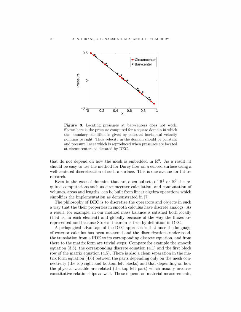
6.6. Circumcenter versus barycenter. One of the main focuses of thispaper is on structure preserving numerical methods, generated by a system-atic application of DEC. The proposed method has both local and globalmass balance properties. In addition, we show that the proposed methodcan also exactly represent linear variation of pressure within a domain. Wealso highlight the need for careful choice of locations for the pressure to getbetter numerical solutions. DEC naturally provides the locations of pres-sure that conserve local and global mass balance, and also exactly representlinear variation of pressure. In DEC, for each element, pressure is locatedat circumcenter. The fact that each (n − 1)-simplex and its circumcentricdual edge are orthogonal is important here. One common choice used inthe literature as location points for pressure are barycenters. In Figure 3we show that choice of barycenter cannot exactly represent linear variationof pressure (along with local and global mass balance) whereas location ofpressure at circumcenter can. This also illustrates how a geometrical view ofPDEs can provide good insights into developing novel structure preservingnumerical methods.

7. Conclusions and Future Work

Our goal in this paper has been to introduce a numerical method for Darcyflow derived using discrete exterior calculus (DEC). We have shown that thisapproach results in a unified derivation of methods for both two- and three-dimensions. We have also demonstrated the numerical performance of thesemethods. For example, the method is shown to pass several patch and otherstandard test problems in both two and three dimensions. Our DEC basedapproach is intrinsic, in the sense that it involves quantities and operations


0 0.2 0.4 0.6 0.8 1−0.5

0

0.5

X

Pre

ssur

e

CircumcenterBarycenter

Figure 3. Locating pressures at barycenters does not work.Shown here is the pressure computed for a square domain in whichthe boundary condition is given by constant horizontal velocitypointing to right. Thus velocity in the domain should be constantand pressure linear which is reproduced when pressures are locatedat circumcenters as dictated by DEC.

that do not depend on how the mesh is embedded in R3. As a result, itshould be easy to use the method for Darcy flow on a curved surface using awell-centered discretization of such a surface. This is one avenue for futureresearch.

Even in the case of domains that are open subsets of R2 or R3 the re-quired computations such as circumcenter calculation, and computation ofvolumes, areas and lengths, can be built from linear algebra operations whichsimplifies the implementation as demonstrated in [7].

The philosophy of DEC is to discretize the operators and objects in sucha way that the their properties in smooth calculus have discrete analogs. Asa result, for example, in our method mass balance is satisfied both locally(that is, in each element) and globally because of the way the fluxes arerepresented and because Stokes’ theorem is true by definition in DEC.

A pedagogical advantage of the DEC approach is that once the languageof exterior calculus has been mastered and the discretizations understood,the translation from a PDE to its corresponding discrete equation, and fromthere to the matrix form are trivial steps. Compare for example the smoothequation (3.8), the corresponding discrete equation (4.1) and the first blockrow of the matrix equation (4.5). There is also a clean separation in the ma-trix form equation (4.6) between the parts depending only on the mesh con-nectivity (the top right and bottom left blocks) and that depending on howthe physical variable are related (the top left part) which usually involvesconstitutive relationships as well. These depend on material measurements,


and hence the inaccuracies of measurement of material properties does notcorrupt that part of the matrix that is topological. In this aspect our methodshares this good property of some mixed finite element method formulations.

In addition to applying DEC to Darcy flow, in this paper we have alsodeveloped a discretization of Hodge star for non-homogeneous medium. Weused this in examples in which the permeability varies across the mesh, eitheralong the flow or transversal to the flow. This discretization of a spatiallyvarying Hodge star should be useful in other PDEs as well.

There are many avenues for future research even within Darcy flow. Flowon curved surfaces has already been mentioned before. Another direction forfurther work is the proper DEC discretization of anisotropic permeability.It is also possible to remove the requirement of using well-centered trian-gulations and this needs to be explored further too. Finally the numericalanalysis of convergence and stability properties remains to be done.

Acknowledgments

The research of ANH and JHC was supported by the National ScienceFoundation with an NSF CAREER Award (Grant No. DMS-0645604).The research of KBN was supported in part by the Department of En-ergy through a SciDAC-2 project (Grant No. DOE DE-FC02-07ER64323).ANH would like to thank his student Evan VanderZee for help in creatingmany of the well-centered meshes in this paper. The authors would like tothank Prof. Albert Valocchi and Prof. Arif Masud for valuable discussions.The opinions expressed in this paper are those of the authors and do notnecessarily reflect that of the sponsors.

References

[1] Abraham, R., Marsden, J. E., and Ratiu, T. Manifolds, TensorAnalysis, and Applications, second ed. Springer–Verlag, New York,1988.

[2] Achdou, Y., Bernardi, C., and Coquela, F. A priori and a pos-teriori analysis of finite volume discretizations of Darcy’s equations.Numerische Mathematik 96 (2003), 17–42.

[3] Arnold, D. N., Bochev, P. B., Lehoucq, R. B., Nicolaides,R. A., and Shashkov, M., Eds. Compatible Spatial Discretizations,vol. 142 of The IMA Volumes in Mathematics and its Applications.Springer New York, 2006. doi:10.1007/0-387-38034-5.

[4] Arnold, D. N., Falk, R. S., and Winther, R. Finite element exte-rior calculus, homological techniques, and applications. In Acta Numer-ica, A. Iserles, Ed., vol. 15. Cambridge University Press, 2006, pp. 1–155. URL http://www.ima.umn.edu/~arnold/papers/acta.pdf.

[5] Arnold, V. I. Mathematical Methods of Classical Mechanics, sec-ond ed. Springer–Verlag, New York, 1989. Translated from the Russianby K. Vogtmann and A. Weinstein.

http://dx.doi.org/10.1007/0-387-38034-5

http://www.ima.umn.edu/~arnold/papers/acta.pdf


[6] Babuska, I., and Narasimhan, R. The Babuska-Brezzi condi-tion and the patch test: an example. Computer Methods in Ap-plied Mechanics and Engineering 140, 1-2 (January 1997), 183–199.doi:10.1016/S0045-7825(96)01058-4.

[7] Bell, N., and Hirani, A. N. PyDEC: Algorithms and software forDiscrete Exterior Calculus. In preparation., 2008.

[8] Benzi, M., Golub, G. H., and Liesen, J. Numerical solution ofsaddle point problems. Acta Numerica 14 (2005), 1–137.

[9] Bochev, P., and Dohrmann, C. A computational study of sta-bilized, low-order C0 finite element approximations of Darcy equa-tions. Computational Mechanics 38, 4-5 (2006), 323–333. doi:10.1007/s00466-006-0036-y.

[10] Bochev, P. B., and Hyman, J. M. Principles of mimetic dis-cretizations of differential operators. In Compatible Spatial Discretiza-tions, D. N. Arnold, P. B. Bochev, R. B. Lehoucq, R. A. Nicolaides,and M. Shashkov, Eds., vol. 142 of The IMA Volumes in Mathemat-ics and its Applications. Springer, Berlin, 2006, pp. 89–119. doi:10.1007/0-387-38034-5.

[11] Bossavit, A. Mixed finite elements and the complex of Whitney forms.In The Mathematics of Finite Elements and Applications VI, J. White-man, Ed. Academic Press, 1988, pp. 137–144.

[12] Bossavit, A. A rationale for “edge elements” in 3-D fields computa-tions. IEEE Trans. Mag. 24, 1 (January 1988), 74–79.

[13] Bossavit, A. Whitney forms : A class of finite elements for three-dimensional computations in electromagnetism. IEE Proceedings 135,Part A, 8 (November 1988), 493–500.

[14] Bossavit, A. Computational Electromagnetism : Variational Formu-lations, Complementarity, Edge Elements. Academic Press, 1998.

[15] Bossavit, A. On the geometry of electromagnetism (4): Maxwell’shouse. Journal of the Japan Society of Applied Electromagnetics 6, 4(1998), 318–326.

[16] Braess, D. Finite Elements: Theory, Fast Solvers, and Applicationsin Solid Mechanics, third ed. Cambridge University Press, Cambridge,2007. Translated from the 1992 German edition by Larry L. Schumaker.

[17] Brezzi, F., Douglas, J., and Marini, L. D. Two families of mixedfinite elements for second order elliptic problems. Numerische Mathe-matik 47, 2 (June 1985), 217–235. doi:10.1007/BF01389710.

[18] Brezzi, F., and Fortin, M. Mixed and hybrid finite element methods,volume 15 of Springer series in computational mathematics. Springer-Verlag, New York, 1991.

[19] Chen, Z. Finite Element Methods and Their Applications. ScientificComputation. Springer, 2005.

[20] Chou, S., and Vassilevski, P. A general mixed covolume frameworkfor constructing conservative schemes for elliptic problems. Mathemat-ics of Computation 68, 227 (1999), 991–1011.

http://dx.doi.org/10.1016/S0045-7825(96)01058-4

http://dx.doi.org/10.1007/s00466-006-0036-y

http://dx.doi.org/10.1007/s00466-006-0036-y

http://dx.doi.org/10.1007/0-387-38034-5

http://dx.doi.org/10.1007/0-387-38034-5

http://dx.doi.org/10.1007/BF01389710


[21] Chou, S.-H., Kwak, D. Y., and Vassilevski, P. S. Mixed covolumemethods for elliptic problems on triangular grids. SIAM Journal onNumerical Analysis 35, 5 (1998), 1850–1861. URL http://www.jstor.org/stable/2587277.

[22] Desbrun, M., Hirani, A. N., Leok, M., and Marsden, J. E. Dis-crete exterior calculus. arXiv:math.DG/0508341 (August 2005). URLhttp://arxiv.org/pdf/math.DG/0508341.

[23] Desbrun, M., Kanso, E., and Tong, Y. Discrete differential formsfor computational modeling. In Discrete Differential Geometry, A. I.Bobenko, J. M. Sullivan, P. Schroder, and G. M. Ziegler, Eds., vol. 38of Oberwolfach Seminars. Birkhauser Basel, 2008, pp. 287–324. doi:10.1007/978-3-7643-8621-4_16.

[24] Dodziuk, J. Finite-difference approach to the Hodge theory of har-monic forms. Amer. J. Math. 98, 1 (1976), 79–104.

[25] Elcott, S., Tong, Y., Kanso, E., Schroder, P., and Desbrun,M. Stable, circulation-preserving, simplicial fluids. ACM Transac-tions on Graphics 26, 1 (2007), 4. doi:http://doi.acm.org/10.1145/1189762.1189766.

[26] Erten, H., and Ungor, A. Computing acute and non-obtuse trian-gulations. In Proceedings of the 19th Canadian Conference on Compu-tational Geometry (CCCG2007) (August 20–22 2007).

[27] Hildebrandt, K., Polthier, K., and Wardetzky, M. On theconvergence of metric and geometric properties of polyhedral surfaces.Geometriae Dedicata 123, 1 (December 2006), 89–112. doi:10.1007/s10711-006-9109-5.

[28] Hirani, A. N. Discrete Exterior Calculus. PhD thesis, CaliforniaInstitute of Technology, May 2003. URL http://resolver.caltech.edu/CaltechETD:etd-05202003-095403.

[29] Hughes, T. J. R., Masud, A., and Wan, J. A stabilized mixeddiscontinuous Galerkin method for Darcy flow. Computer Methods inApplied Mechanics and Engineering 195 (2006), 3347–3381.

[30] Hyman, J. M., and Shashkov, M. Natural discretizations for thedivergence, gradient, and curl on logically rectangular grids. Comput.Math. Appl. 33, 4 (1997), 81–104.

[31] Irons, B., and Loikkanen, M. An engineers’ defence of the patchtest. International Journal for Numerical Methods in Engineering 19,9 (1983), 1391–1401. doi:10.1002/nme.1620190908.

[32] Lipnikov, K., Shashkov, M., and Svyatskiy, D. The mimetic fi-nite difference discretization of diffusion problem on unstructured poly-hedral meshes. Journal of Computational Physics 211, 2 (January2006), 473–491. doi:10.1016/j.jcp.2005.05.028.

[33] Lipnikov, K., Shashkov, M., Svyatskiy, D., and Vassilevski, Y.Monotone finite volume schemes for diffusion equations on unstructuredtriangular and shape-regular polygonal meshes. Journal of Computa-tional Physics 227, 1 (492–512 2007). doi:10.1016/j.jcp.2007.08.

http://www.jstor.org/stable/2587277


http://arxiv.org/pdf/math.DG/0508341

http://dx.doi.org/10.1007/978-3-7643-8621-4_16

http://dx.doi.org/10.1007/978-3-7643-8621-4_16

http://dx.doi.org/http://doi.acm.org/10.1145/1189762.1189766

http://dx.doi.org/http://doi.acm.org/10.1145/1189762.1189766

http://dx.doi.org/10.1007/s10711-006-9109-5

http://dx.doi.org/10.1007/s10711-006-9109-5

http://resolver.caltech.edu/CaltechETD:etd-05202003-095403

http://resolver.caltech.edu/CaltechETD:etd-05202003-095403

http://dx.doi.org/10.1002/nme.1620190908

http://dx.doi.org/10.1016/j.jcp.2005.05.028



008.[34] Maehara, H. Acute triangulations of polygons. European Journal of

Combinatorics 23, 1 (2002), 45–55.[35] Masud, A., and Hughes, T. J. R. A stabilized mixed finite element

method for Darcy flow. Computer Methods Applied Mechanics andEngineering 191 (2002), 4341–4370. doi:10.1016/S0045-7825(02)00371-7.

[36] Munkres, J. R. Elements of Algebraic Topology. Addison–WesleyPublishing Company, Menlo Park, 1984.

[37] Nakshatrala, K. B., Masud, A., and Hjelmstad, K. D. Onfinite element formulations for nearly incompressible linear elasticity.Computational Mechanics 41 (2008), 547–561.

[38] Nakshatrala, K. B., Turner, D. Z., Hjelmstad, K. D., andMasud, A. A mixed stabilized finite element formulation for Darcyflow based on a multiscale decomposition of the solution. ComputerMethods in Applied Mechanics and Engineering 195 (2006), 4036–4049.

[39] Nedelec, J. C. Mixed finite elements in R3. Numerische Mathematik35, 3 (1980), 315–341. doi:10.1007/BF01396415.

[40] Nicolaides, R. A. Direct discretization of planar div-curl problems.SIAM Journal on Numerical Analysis 29, 1 (1992), 32–56. URL http://www.jstor.org/stable/2158074.

[41] Nicolaides, R. A., and Wu, X. Covolume solutions of three-dimensional div-curl equations. SIAM Journal on Numerical Analysis34, 6 (1997), 2195–2203.

[42] Perot, J., and Subramanian, V. Discrete calculus methods fordiffusion. Journal of Computational Physics 224, 1 (2007), 59–81. doi:10.1016/j.jcp.2006.12.022.

[43] Raviart, P.-A., and Thomas, J. M. A mixed finite element methodfor 2nd order elliptic problems. In Mathematical aspects of finite elementmethods (Proc. Conf., Consiglio Naz. delle Ricerche (C.N.R.), Rome,1975), Lecture Notes in Math., Vol. 606. Springer, Berlin, 1977, pp. 292–315.

[44] Vanderzee, E., Hirani, A. N., and Guoy, D. Triangulation ofsimple 3d shapes with well-centered tetrahedra. Tech. Rep. UIUCDCS-R-2008-2970, Department of Computer Science, University of Illinoisat Urbana-Champaign, 2008. Also available as a preprint at arXiv asarXiv:0806.2332v1 [cs.CG]. URL http://arxiv.org/abs/0806.2332.

[45] Vanderzee, E., Hirani, A. N., Guoy, D., and Ramos, E. Well-centered planar triangulation – An iterative approach. In Proceedingsof 16th International Meshing Roundtable (Seattle, Washington, Octo-ber 14–17 2007), M. L. Brewer and D. Marcum, Eds., Springer Berlin,pp. 121–138. doi:10.1007/978-3-540-75103-8.

[46] Vanderzee, E., Hirani, A. N., Guoy, D., and Ramos, E.



http://dx.doi.org/10.1016/S0045-7825(02)00371-7

http://dx.doi.org/10.1016/S0045-7825(02)00371-7

http://dx.doi.org/10.1007/BF01396415





http://arxiv.org/abs/0806.2332

http://dx.doi.org/10.1007/978-3-540-75103-8


Well-centered triangulation. Tech. Rep. UIUCDCS-R-2008-2936, De-partment of Computer Science, University of Illinois at Urbana-Champaign, February 2008. Also available as a preprint at arXiv asarXiv:0802.2108v1 [cs.CG]. URL http://arxiv.org/abs/0802.2108.

[47] Wardetzky, M. Convergence of the cotangent formula: Anoverview. In Discrete Differential Geometry, A. I. Bobenko, J. M.Sullivan, P. Schroder, and G. M. Ziegler, Eds., vol. 38 of Oberwol-fach Seminars. Birkhauser Basel, 2008, pp. 275–286. doi:10.1007/978-3-7643-8621-4_15.

[48] Whitney, H. Geometric Integration Theory. Princeton UniversityPress, Princeton, N. J., 1957.

[49] Yuan, L. Acute triangulations of polygons. Discrete and Computa-tional Geometry 34, 4 (2005), 697–706.

Correspondence to: Professor Anil N. Hirani, Department of ComputerScience, University of Illinois at Urbana-Champaign, 201 N. Goodwin Ave.,Urbana, IL 61801.

E-mail address: [email protected]

URL: http://www.cs.uiuc.edu/hirani

Dr. Kalyana Babu Nakshatrala, Department of Civil and EnvironmentalEngineering, 2524 Hydrosystems Laboratory, University of Illinois at Urbana-Champaign, Urbana, IL 61801.


Jehanzeb H. Chaudhry, Department of Computer Science, University ofIllinois at Urbana-Champaign, 201 N. Goodwin Ave., Urbana, IL 61801.


http://arxiv.org/abs/0802.2108

http://dx.doi.org/10.1007/978-3-7643-8621-4_15

http://dx.doi.org/10.1007/978-3-7643-8621-4_15

mailto:[email protected]

http://www.cs.uiuc.edu/hirani


0 0.2 0.4 0.6 0.8 1 1.20

0.1

0.2

0.3

0.4

0.5

0.6

0.7

0.8

0.9

1

0 0.2 0.4 0.6 0.8 10

0.1

0.2

0.3

0.4

0.5

0.6

0.7

0.8

0.9

x

Pre

ssur

e

DECAnalytical

−1 −0.5 0 0.5 1

−0.8

−0.6

−0.4

−0.2

0

0.2

0.4

0.6

0.8

−0.6 −0.4 −0.2 0 0.2 0.4 0.60

0.1

0.2

0.3

0.4

0.5

0.6

0.7

0.8

0.9

1

x

Pre

ssur

e

DECAnalytical

Figure 4. Results from patch tests. The boundary conditions areobtained from a velocity of 1 in positive x direction. Thus, for thesquare domain, in equation (3.3), ψ = −1 on left edge, 1 on rightedge, and 0 on top and bottom edges. For both the square andhexagon domains it is also given is that φ = 0 in (3.2), constantsk = 1, µ = 1 and external body force acceleration g = 0 in (3.1).The pressure should be linear as shown in the right figures. Theleft figures show that the velocity is constant, as expected. Thevelocity displayed is interpolated from the flux through each edge,using Whitney 1-form and sampled and converted to a vector.


0 0.2 0.4 0.6 0.8 10

0.1

0.2

0.3

0.4

0.5

0.6

0.7

0.8

0.9

1

Figure 5. Patch test with larger mesh and with the same bound-ary conditions, parameters and other data as the square in Fig-ure 4.


0 0.2 0.4 0.6 0.8 10

0.1

0.2

0.3

0.4

0.5

0.6

0.7

0.8

0.9

1

X

Y

−1

−0.8

−0.6

−0.4

−0.2

0

0.2

0.4

0.6

0.8

1

0 0.2 0.4 0.6 0.8 10

0.1

0.2

0.3

0.4

0.5

0.6

0.7

0.8

0.9

1

0 0.2 0.4 0.6 0.8 10

0.1

0.2

0.3

0.4

0.5

0.6

0.7

0.8

0.9

1

X

Y

−0.8

−0.6

−0.4

−0.2

0

0.2

0.4

0.6

0.8

1

0 0.2 0.4 0.6 0.8 10

0.1

0.2

0.3

0.4

0.5

0.6

0.7

0.8

0.9

1

Figure 6. Comparison of analytically known solution with a solu-tion computed using the method developed here. The top left fig-ure shows the pressure part of the analytical solution to the Darcylaw problem with k = 1, µ = 1, g = 0, and φ = 2π2 cos(πx) cos(πy).This implies p = cos(πx) cos(πy) which is shown overlaid on themesh. In the left bottom figure we show the pressure computedwith the numerical method proposed here. Each triangle is coloredby the pressure at its circumcenter. The top right figure shows theanalytically computed vector field, and the numerically computedvector field is shown in the right bottom figure, which is obtainedfrom the flux by interpolation of 1-forms.


0 0.2 0.4 0.6 0.8 1

−0.1

0

0.1

0.2

0.3

0.4

0.5

0.6

0 0.1 0.2 0.3 0.4 0.5 0.6 0.7 0.8 0.9 10

0.1

0.2

0.3

0.4

0.5

0.6

0.7

0.8

0.9

1

X

Pre

ssur

e

k1 = 1, k

2 = 1

k1 = 1, k

2 = 10

k1 = 1, k

2 = 2

k1 = 1, k

2 = 100

Figure 7. In this test the left and right halves of the mesh aregiven different permeabilities, k1 on the left and k2 on right. Thusthe permeability jumps across the middle vertical edge at x = 0.5.The values that we use for (k1, k2) are (1, 1), (1, 2), (1, 10) and(1, 100). The boundary condition is derived from velocity (1, 0) asin Figure 4. The top figure shows the computed velocity interpo-lated from flux for k1 = 1 and k2 = 10. All other value pairs alsoresult in a constant velocity solution as expected. The pressureis piecewise linear with a jump at the discontinuity at x = 0.5 asshown in the bottom figure.


0 0.2 0.4 0.6 0.8 10

0.2

0.4

0.6

0.8

1

0 0.2 0.4 0.6 0.8 10

0.2

0.4

0.6

0.8

1

Figure 8. Layered medium with 2 different permeability patterns.The domain has 5 layers with alternating permeability. In the topfigure the permeability k, from bottom layer to top is 5, 10, 5, 10and 5. In the bottom figure the permeability k is 1, 10, 1, 10 and1. The computed flux is visualized as a vector field.


0 0.2 0.4 0.6 0.8 1−0.8

−0.6

−0.4

−0.2

0

0.2

0.4

0.6

X

Pre

ssur

e

0 0.2 0.4 0.6 0.8 1−0.8

−0.6

−0.4

−0.2

0

0.2

0.4

0.6

X

Pre

ssur

e

Figure 9. Pressure for the layered medium show in Figure 8. Thepressure is linear as expected. The top and bottom figures corre-spond to the top and bottom figures in Figure 8.


!1 !0.5 0 0.5 1!1

!0.5

0

0.5

1

x

Pre

ssu

re

DEC

Analytical

Figure 10. Patch test in 3D. The mesh shown has 16 tetrahedra,each of which is well-centered. Each triangle in the mesh is alsowell-centered. The fluid velocity on the boundary is from negativex to positive x direction, with no y or z components. The fluxes (2-cochains) across the internal faces are computed using our methodand interpolated using the Whitney map. This is then sampledat the circumcenters, converted into a vector field and plotted asarrows.


0

0.5

1

0

0.5

10

0.2

0.4

0.6

0.8

1

xy

z

0 0.2 0.4 0.6 0.8 1−0.8

−0.7

−0.6

−0.5

−0.4

−0.3

−0.2

−0.1

0

0.1

0.2

0.3

x

Pre

ssur

e

DECAnalytical

0 0.2 0.4 0.6 0.8 1−2

−1.5

−1

−0.5

0

0.5

1

1.5x 10

−13

x

Rel

ativ

e E

rror

in P

ress

ure

Figure 11. Patch test on a cube. The mesh used for this cube has244 tetrahedra, each of which is well-centered. Each triangle in themesh is also well-centered. For clarity, the tetrahedra in the cubehave not been shown. The fluid velocity on the boundary is fromnegative x to positive x direction, with no y or z components. Thefluxes (2-cochains) across the internal faces are computed usingour method and interpolated using the Whitney map. This is thensampled at the circumcenters, converted into a vector field andplotted as arrows. In the relative error plot for pressure, the datawith 0 exact pressure has been removed.

numerical method for darcy flow derived using discrete exterior calculus

Documents