numerical mathematics -...
TRANSCRIPT
Numerical Mathematics
Alfio QuarteroniRiccardo SaccoFausto Saleri
Springer

Texts in Applied Mathematicsm37
SpringerNew YorkBerlinHeidelbergBarcelonaHong KongLondonMilanParisSingaporeTokyo
EditorsJ.E. Marsden
L. SirovichM. Golubitsky
W. Jäger
AdvisorsG. Iooss
P. HolmesD. Barkley
M. DellnitzP. Newton


Alfio QuarteroniMMRiccardo SaccoFausto Saleri
123
Numerical Mathematics
With 134 Illustrations

Alfio QuarteroniDepartment of MathematicsEcole PolytechniqueMFederale de Lausanne CH-1015 [email protected]
Riccardo SaccoDipartimento di MatematicaPolitecnico di MilanoPiazza Leonardo da Vinci 3220133 [email protected]
Fausto SaleriDipartimento di Matematica,M“F. Enriques”Università degli Studi diMMilanoVia Saldini 5020133 [email protected]
Series Editors
J.E. Marsden Control and Dynamical Systems, 107–81California Institute of TechnologyPasadena, CA 91125USA
M. GolubitskyDepartment of MathematicsUniversity of HoustonHouston, TX 77204-3476USA
L. SirovichDivision of Applied MathematicsBrown University Providence, RI 02912USA
W. JagerDepartment of Applied MathematicsUniversit at HeidelbergIm Neuenheimer Feld 29469120 Heidelberg Germany
Library of Congress Cataloging-in-Publication DataQuarteroni, Alfio.
Numerical mathematics/Alfio Quarteroni, Riccardo Sacco, Fausto Saleri.p.Mcm. — (Texts in applied mathematics; 37)
Includes bibliographical references and index.ISBN 0-387-98959-5 (alk. paper)1. Numerical analysis.MI. Sacco, Riccardo.MII. Saleri, Fausto.MIII. Title.MIV. Series.
I. Title.MMII. Series.QA297.Q83M2000519.4—dc21 99-059414
© 2000 Springer-Verlag New York, Inc.All rights reserved. This work may not be translated or copied in whole or in part withoutthe written permission of the publisher (Springer-Verlag New York, Inc., 175 Fifth Avenue,New York, NY 10010, USA), except for brief excerpts in connection with reviews or scholarlyanalysis. Use in connection with any form of information storage and retrieval, electronicadaptation, computer software, or by similar or dissimilar methodology now known or heraf-ter developed is forbidden.The use of general descriptive names, trade names, trademarks, etc., in this publication, evenif the former are not especially identified, is not to be taken as a sign that such names, asunderstood by the Trade Marks and Merchandise Marks Act, may accordingly be used freelyby anyone.
ISBN 0-387-98959-5nSpringer-VerlagnNew YorknBerlinnHeidelbergMSPIN 10747955
Mathematics Subject Classification (1991): 15-01, 34-01, 35-01, 65-01

Preface
Numerical mathematics is the branch of mathematics that proposes, de-velops, analyzes and applies methods from scientific computing to severalfields including analysis, linear algebra, geometry, approximation theory,functional equations, optimization and di!erential equations. Other disci-plines such as physics, the natural and biological sciences, engineering, andeconomics and the financial sciences frequently give rise to problems thatneed scientific computing for their solutions.
As such, numerical mathematics is the crossroad of several disciplines ofgreat relevance in modern applied sciences, and can become a crucial toolfor their qualitative and quantitative analysis. This role is also emphasizedby the continual development of computers and algorithms, which make itpossible nowadays, using scientific computing, to tackle problems of sucha large size that real-life phenomena can be simulated providing accurateresponses at a!ordable computational cost.
The corresponding spread of numerical software represents an enrichmentfor the scientific community. However, the user has to make the correctchoice of the method (or the algorithm) which best suits the problem athand. As a matter of fact, no black-box methods or algorithms exist thatcan e!ectively and accurately solve all kinds of problems.
One of the purposes of this book is to provide the mathematical foun-dations of numerical methods, to analyze their basic theoretical proper-ties (stability, accuracy, computational complexity), and demonstrate theirperformances on examples and counterexamples which outline their pros
viii Preface
and cons. This is done using the MATLAB! 1 software environment. Thischoice satisfies the two fundamental needs of user-friendliness and wide-spread di!usion, making it available on virtually every computer.
Every chapter is supplied with examples, exercises and applications ofthe discussed theory to the solution of real-life problems. The reader isthus in the ideal condition for acquiring the theoretical knowledge that isrequired to make the right choice among the numerical methodologies andmake use of the related computer programs.
This book is primarily addressed to undergraduate students, with partic-ular focus on the degree courses in Engineering, Mathematics, Physics andComputer Science. The attention which is paid to the applications and therelated development of software makes it valuable also for graduate stu-dents, researchers and users of scientific computing in the most widespreadprofessional fields.
The content of the volume is organized into four parts and 13 chapters.Part I comprises two chapters in which we review basic linear algebra and
introduce the general concepts of consistency, stability and convergence ofa numerical method as well as the basic elements of computer arithmetic.
Part II is on numerical linear algebra, and is devoted to the solution oflinear systems (Chapters 3 and 4) and eigenvalues and eigenvectors com-putation (Chapter 5).
We continue with Part III where we face several issues about functionsand their approximation. Specifically, we are interested in the solution ofnonlinear equations (Chapter 6), solution of nonlinear systems and opti-mization problems (Chapter 7), polynomial approximation (Chapter 8) andnumerical integration (Chapter 9).
Part IV, which is the more demanding as a mathematical background, isconcerned with approximation, integration and transforms based on orthog-onal polynomials (Chapter 10), solution of initial value problems (Chap-ter 11), boundary value problems (Chapter 12) and initial-boundary valueproblems for parabolic and hyperbolic equations (Chapter 13).
Part I provides the indispensable background. Each of the remainingParts has a size and a content that make it well suited for a semestercourse.
A guideline index to the use of the numerous MATLAB Programs de-veloped in the book is reported at the end of the volume. These programsare also available at the web site address:
http://www1.mate.polimi.it/ calnum/programs.htmlFor the reader’s ease, any code is accompanied by a brief description of
its input/output parameters.We express our thanks to the sta! at Springer-Verlag New York for their
expert guidance and assistance with editorial aspects, as well as to Dr.
1MATLAB is a registered trademark of The MathWorks, Inc.

Preface ix
Martin Peters from Springer-Verlag Heidelberg and Dr. Francesca Bonadeifrom Springer-Italia for their advice and friendly collaboration all alongthis project.
We gratefully thank Professors L. Gastaldi and A. Valli for their usefulcomments on Chapters 12 and 13.
We also wish to express our gratitude to our families for their forbearanceand understanding, and dedicate this book to them.
Lausanne, Switzerland Alfio QuarteroniMilan, Italy Riccardo SaccoMilan, Italy Fausto SaleriJanuary 2000

Contents
Series Preface v
Preface vii
PART I: Getting Started
1. Foundations of Matrix Analysis 11.1 Vector Spaces . . . . . . . . . . . . . . . . . . . . . . . . . 11.2 Matrices . . . . . . . . . . . . . . . . . . . . . . . . . . . . 31.3 Operations with Matrices . . . . . . . . . . . . . . . . . . . 5
1.3.1 Inverse of a Matrix . . . . . . . . . . . . . . . . . . 61.3.2 Matrices and Linear Mappings . . . . . . . . . . . 71.3.3 Operations with Block-Partitioned Matrices . . . . 7
1.4 Trace and Determinant of a Matrix . . . . . . . . . . . . . 81.5 Rank and Kernel of a Matrix . . . . . . . . . . . . . . . . 91.6 Special Matrices . . . . . . . . . . . . . . . . . . . . . . . . 10
1.6.1 Block Diagonal Matrices . . . . . . . . . . . . . . . 101.6.2 Trapezoidal and Triangular Matrices . . . . . . . . 111.6.3 Banded Matrices . . . . . . . . . . . . . . . . . . . 11
1.7 Eigenvalues and Eigenvectors . . . . . . . . . . . . . . . . 121.8 Similarity Transformations . . . . . . . . . . . . . . . . . . 141.9 The Singular Value Decomposition (SVD) . . . . . . . . . 161.10 Scalar Product and Norms in Vector Spaces . . . . . . . . 171.11 Matrix Norms . . . . . . . . . . . . . . . . . . . . . . . . . 21

xii Contents
1.11.1 Relation Between Norms and theSpectral Radius of a Matrix . . . . . . . . . . . . . 25
1.11.2 Sequences and Series of Matrices . . . . . . . . . . 261.12 Positive Definite, Diagonally Dominant and M-Matrices . 271.13 Exercises . . . . . . . . . . . . . . . . . . . . . . . . . . . . 30
2. Principles of Numerical Mathematics 332.1 Well-Posedness and Condition Number of a Problem . . . 332.2 Stability of Numerical Methods . . . . . . . . . . . . . . . 37
2.2.1 Relations Between Stability and Convergence . . . 402.3 A priori and a posteriori Analysis . . . . . . . . . . . . . . 412.4 Sources of Error in Computational Models . . . . . . . . . 432.5 Machine Representation of Numbers . . . . . . . . . . . . 45
2.5.1 The Positional System . . . . . . . . . . . . . . . . 452.5.2 The Floating-Point Number System . . . . . . . . 462.5.3 Distribution of Floating-Point Numbers . . . . . . 492.5.4 IEC/IEEE Arithmetic . . . . . . . . . . . . . . . . 492.5.5 Rounding of a Real Number in Its
Machine Representation . . . . . . . . . . . . . . . 502.5.6 Machine Floating-Point Operations . . . . . . . . . 52
2.6 Exercises . . . . . . . . . . . . . . . . . . . . . . . . . . . . 54
PART II: Numerical Linear Algebra
3. Direct Methods for the Solution of Linear Systems 573.1 Stability Analysis of Linear Systems . . . . . . . . . . . . 58
3.1.1 The Condition Number of a Matrix . . . . . . . . 583.1.2 Forward a priori Analysis . . . . . . . . . . . . . . 603.1.3 Backward a priori Analysis . . . . . . . . . . . . . 633.1.4 A posteriori Analysis . . . . . . . . . . . . . . . . . 64
3.2 Solution of Triangular Systems . . . . . . . . . . . . . . . 653.2.1 Implementation of Substitution Methods . . . . . 653.2.2 Rounding Error Analysis . . . . . . . . . . . . . . 673.2.3 Inverse of a Triangular Matrix . . . . . . . . . . . 67
3.3 The Gaussian Elimination Method (GEM) andLU Factorization . . . . . . . . . . . . . . . . . . . . . . . 683.3.1 GEM as a Factorization Method . . . . . . . . . . 723.3.2 The E!ect of Rounding Errors . . . . . . . . . . . 763.3.3 Implementation of LU Factorization . . . . . . . . 773.3.4 Compact Forms of Factorization . . . . . . . . . . 78
3.4 Other Types of Factorization . . . . . . . . . . . . . . . . . 793.4.1 LDMT Factorization . . . . . . . . . . . . . . . . . 793.4.2 Symmetric and Positive Definite Matrices:
The Cholesky Factorization . . . . . . . . . . . . . 803.4.3 Rectangular Matrices: The QR Factorization . . . 82
Contents xiii
3.5 Pivoting . . . . . . . . . . . . . . . . . . . . . . . . . . . . 853.6 Computing the Inverse of a Matrix . . . . . . . . . . . . . 893.7 Banded Systems . . . . . . . . . . . . . . . . . . . . . . . . 90
3.7.1 Tridiagonal Matrices . . . . . . . . . . . . . . . . . 913.7.2 Implementation Issues . . . . . . . . . . . . . . . . 92
3.8 Block Systems . . . . . . . . . . . . . . . . . . . . . . . . . 933.8.1 Block LU Factorization . . . . . . . . . . . . . . . 943.8.2 Inverse of a Block-Partitioned Matrix . . . . . . . 953.8.3 Block Tridiagonal Systems . . . . . . . . . . . . . . 95
3.9 Sparse Matrices . . . . . . . . . . . . . . . . . . . . . . . . 973.9.1 The Cuthill-McKee Algorithm . . . . . . . . . . . 983.9.2 Decomposition into Substructures . . . . . . . . . 1003.9.3 Nested Dissection . . . . . . . . . . . . . . . . . . . 103
3.10 Accuracy of the Solution Achieved Using GEM . . . . . . 1033.11 An Approximate Computation of K(A) . . . . . . . . . . . 1063.12 Improving the Accuracy of GEM . . . . . . . . . . . . . . 109
3.12.1 Scaling . . . . . . . . . . . . . . . . . . . . . . . . 1103.12.2 Iterative Refinement . . . . . . . . . . . . . . . . . 111
3.13 Undetermined Systems . . . . . . . . . . . . . . . . . . . . 1123.14 Applications . . . . . . . . . . . . . . . . . . . . . . . . . . 115
3.14.1 Nodal Analysis of a Structured Frame . . . . . . . 1153.14.2 Regularization of a Triangular Grid . . . . . . . . 118
3.15 Exercises . . . . . . . . . . . . . . . . . . . . . . . . . . . . 121
4. Iterative Methods for Solving Linear Systems 1234.1 On the Convergence of Iterative Methods . . . . . . . . . . 1234.2 Linear Iterative Methods . . . . . . . . . . . . . . . . . . . 126
4.2.1 Jacobi, Gauss-Seidel and Relaxation Methods . . . 1274.2.2 Convergence Results for Jacobi and
Gauss-Seidel Methods . . . . . . . . . . . . . . . . 1294.2.3 Convergence Results for the Relaxation Method . 1314.2.4 A priori Forward Analysis . . . . . . . . . . . . . . 1324.2.5 Block Matrices . . . . . . . . . . . . . . . . . . . . 1334.2.6 Symmetric Form of the Gauss-Seidel and
SOR Methods . . . . . . . . . . . . . . . . . . . . . 1334.2.7 Implementation Issues . . . . . . . . . . . . . . . . 135
4.3 Stationary and Nonstationary Iterative Methods . . . . . . 1364.3.1 Convergence Analysis of the Richardson Method . 1374.3.2 Preconditioning Matrices . . . . . . . . . . . . . . 1394.3.3 The Gradient Method . . . . . . . . . . . . . . . . 1464.3.4 The Conjugate Gradient Method . . . . . . . . . . 1504.3.5 The Preconditioned Conjugate Gradient Method . 1564.3.6 The Alternating-Direction Method . . . . . . . . . 158
4.4 Methods Based on Krylov Subspace Iterations . . . . . . . 1594.4.1 The Arnoldi Method for Linear Systems . . . . . . 162

xiv Contents
4.4.2 The GMRES Method . . . . . . . . . . . . . . . . 1654.4.3 The Lanczos Method for Symmetric Systems . . . 167
4.5 The Lanczos Method for Unsymmetric Systems . . . . . . 1684.6 Stopping Criteria . . . . . . . . . . . . . . . . . . . . . . . 171
4.6.1 A Stopping Test Based on the Increment . . . . . 1724.6.2 A Stopping Test Based on the Residual . . . . . . 174
4.7 Applications . . . . . . . . . . . . . . . . . . . . . . . . . . 1744.7.1 Analysis of an Electric Network . . . . . . . . . . . 1744.7.2 Finite Di!erence Analysis of Beam Bending . . . . 177
4.8 Exercises . . . . . . . . . . . . . . . . . . . . . . . . . . . . 179
5. Approximation of Eigenvalues and Eigenvectors 1835.1 Geometrical Location of the Eigenvalues . . . . . . . . . . 1835.2 Stability and Conditioning Analysis . . . . . . . . . . . . . 186
5.2.1 A priori Estimates . . . . . . . . . . . . . . . . . . 1865.2.2 A posteriori Estimates . . . . . . . . . . . . . . . . 190
5.3 The Power Method . . . . . . . . . . . . . . . . . . . . . . 1925.3.1 Approximation of the Eigenvalue of
Largest Module . . . . . . . . . . . . . . . . . . . . 1925.3.2 Inverse Iteration . . . . . . . . . . . . . . . . . . . 1955.3.3 Implementation Issues . . . . . . . . . . . . . . . . 196
5.4 The QR Iteration . . . . . . . . . . . . . . . . . . . . . . . 2005.5 The Basic QR Iteration . . . . . . . . . . . . . . . . . . . . 2015.6 The QR Method for Matrices in Hessenberg Form . . . . . 203
5.6.1 Householder and Givens Transformation Matrices 2045.6.2 Reducing a Matrix in Hessenberg Form . . . . . . 2075.6.3 QR Factorization of a Matrix in Hessenberg Form 2095.6.4 The Basic QR Iteration Starting from
Upper Hessenberg Form . . . . . . . . . . . . . . . 2105.6.5 Implementation of Transformation Matrices . . . . 212
5.7 The QR Iteration with Shifting Techniques . . . . . . . . . 2155.7.1 The QR Method with Single Shift . . . . . . . . . 2155.7.2 The QR Method with Double Shift . . . . . . . . . 218
5.8 Computing the Eigenvectors and the SVD of a Matrix . . 2215.8.1 The Hessenberg Inverse Iteration . . . . . . . . . . 2215.8.2 Computing the Eigenvectors from the
Schur Form of a Matrix . . . . . . . . . . . . . . . 2215.8.3 Approximate Computation of the SVD of a Matrix 222
5.9 The Generalized Eigenvalue Problem . . . . . . . . . . . . 2245.9.1 Computing the Generalized Real Schur Form . . . 2255.9.2 Generalized Real Schur Form of
Symmetric-Definite Pencils . . . . . . . . . . . . . 2265.10 Methods for Eigenvalues of Symmetric Matrices . . . . . . 227
5.10.1 The Jacobi Method . . . . . . . . . . . . . . . . . 2275.10.2 The Method of Sturm Sequences . . . . . . . . . . 230
Contents xv
5.11 The Lanczos Method . . . . . . . . . . . . . . . . . . . . . 2335.12 Applications . . . . . . . . . . . . . . . . . . . . . . . . . . 235
5.12.1 Analysis of the Buckling of a Beam . . . . . . . . . 2365.12.2 Free Dynamic Vibration of a Bridge . . . . . . . . 238
5.13 Exercises . . . . . . . . . . . . . . . . . . . . . . . . . . . . 240
PART III: Around Functions and Functionals
6. Rootfinding for Nonlinear Equations 2456.1 Conditioning of a Nonlinear Equation . . . . . . . . . . . . 2466.2 A Geometric Approach to Rootfinding . . . . . . . . . . . 248
6.2.1 The Bisection Method . . . . . . . . . . . . . . . . 2486.2.2 The Methods of Chord, Secant and Regula Falsi
and Newton’s Method . . . . . . . . . . . . . . . . 2516.2.3 The Dekker-Brent Method . . . . . . . . . . . . . 256
6.3 Fixed-Point Iterations for Nonlinear Equations . . . . . . . 2576.3.1 Convergence Results for
Some Fixed-Point Methods . . . . . . . . . . . . . 2606.4 Zeros of Algebraic Equations . . . . . . . . . . . . . . . . . 261
6.4.1 The Horner Method and Deflation . . . . . . . . . 2626.4.2 The Newton-Horner Method . . . . . . . . . . . . 2636.4.3 The Muller Method . . . . . . . . . . . . . . . . . 267
6.5 Stopping Criteria . . . . . . . . . . . . . . . . . . . . . . . 2696.6 Post-Processing Techniques for Iterative Methods . . . . . 272
6.6.1 Aitken’s Acceleration . . . . . . . . . . . . . . . . 2726.6.2 Techniques for Multiple Roots . . . . . . . . . . . 275
6.7 Applications . . . . . . . . . . . . . . . . . . . . . . . . . . 2766.7.1 Analysis of the State Equation for a Real Gas . . 2766.7.2 Analysis of a Nonlinear Electrical Circuit . . . . . 277
6.8 Exercises . . . . . . . . . . . . . . . . . . . . . . . . . . . . 279
7. Nonlinear Systems and Numerical Optimization 2817.1 Solution of Systems of Nonlinear Equations . . . . . . . . 282
7.1.1 Newton’s Method and Its Variants . . . . . . . . . 2837.1.2 Modified Newton’s Methods . . . . . . . . . . . . . 2847.1.3 Quasi-Newton Methods . . . . . . . . . . . . . . . 2887.1.4 Secant-Like Methods . . . . . . . . . . . . . . . . . 2887.1.5 Fixed-Point Methods . . . . . . . . . . . . . . . . . 290
7.2 Unconstrained Optimization . . . . . . . . . . . . . . . . . 2947.2.1 Direct Search Methods . . . . . . . . . . . . . . . . 2957.2.2 Descent Methods . . . . . . . . . . . . . . . . . . . 3007.2.3 Line Search Techniques . . . . . . . . . . . . . . . 3027.2.4 Descent Methods for Quadratic Functions . . . . . 3047.2.5 Newton-Like Methods for Function Minimization . 3077.2.6 Quasi-Newton Methods . . . . . . . . . . . . . . . 308

xvi Contents
7.2.7 Secant-Like Methods . . . . . . . . . . . . . . . . . 3097.3 Constrained Optimization . . . . . . . . . . . . . . . . . . 311
7.3.1 Kuhn-Tucker Necessary Conditions forNonlinear Programming . . . . . . . . . . . . . . . 313
7.3.2 The Penalty Method . . . . . . . . . . . . . . . . . 3157.3.3 The Method of Lagrange Multipliers . . . . . . . . 317
7.4 Applications . . . . . . . . . . . . . . . . . . . . . . . . . . 3197.4.1 Solution of a Nonlinear System Arising from
Semiconductor Device Simulation . . . . . . . . . . 3207.4.2 Nonlinear Regularization of a Discretization Grid . 323
7.5 Exercises . . . . . . . . . . . . . . . . . . . . . . . . . . . . 325
8. Polynomial Interpolation 3278.1 Polynomial Interpolation . . . . . . . . . . . . . . . . . . . 328
8.1.1 The Interpolation Error . . . . . . . . . . . . . . . 3298.1.2 Drawbacks of Polynomial Interpolation on Equally
Spaced Nodes and Runge’s Counterexample . . . . 3308.1.3 Stability of Polynomial Interpolation . . . . . . . . 332
8.2 Newton Form of the Interpolating Polynomial . . . . . . . 3338.2.1 Some Properties of Newton Divided Di!erences . . 3358.2.2 The Interpolation Error Using Divided Di!erences 337
8.3 Piecewise Lagrange Interpolation . . . . . . . . . . . . . . 3388.4 Hermite-Birko! Interpolation . . . . . . . . . . . . . . . . 3418.5 Extension to the Two-Dimensional Case . . . . . . . . . . 343
8.5.1 Polynomial Interpolation . . . . . . . . . . . . . . 3438.5.2 Piecewise Polynomial Interpolation . . . . . . . . . 344
8.6 Approximation by Splines . . . . . . . . . . . . . . . . . . 3488.6.1 Interpolatory Cubic Splines . . . . . . . . . . . . . 3498.6.2 B-Splines . . . . . . . . . . . . . . . . . . . . . . . 353
8.7 Splines in Parametric Form . . . . . . . . . . . . . . . . . 3578.7.1 Bezier Curves and Parametric B-Splines . . . . . . 359
8.8 Applications . . . . . . . . . . . . . . . . . . . . . . . . . . 3628.8.1 Finite Element Analysis of a Clamped Beam . . . 3638.8.2 Geometric Reconstruction Based on
Computer Tomographies . . . . . . . . . . . . . . . 3668.9 Exercises . . . . . . . . . . . . . . . . . . . . . . . . . . . . 368
9. Numerical Integration 3719.1 Quadrature Formulae . . . . . . . . . . . . . . . . . . . . . 3719.2 Interpolatory Quadratures . . . . . . . . . . . . . . . . . . 373
9.2.1 The Midpoint or Rectangle Formula . . . . . . . . 3739.2.2 The Trapezoidal Formula . . . . . . . . . . . . . . 3759.2.3 The Cavalieri-Simpson Formula . . . . . . . . . . . 377
9.3 Newton-Cotes Formulae . . . . . . . . . . . . . . . . . . . 3789.4 Composite Newton-Cotes Formulae . . . . . . . . . . . . . 383

Contents xvii
9.5 Hermite Quadrature Formulae . . . . . . . . . . . . . . . . 3869.6 Richardson Extrapolation . . . . . . . . . . . . . . . . . . 387
9.6.1 Romberg Integration . . . . . . . . . . . . . . . . . 3899.7 Automatic Integration . . . . . . . . . . . . . . . . . . . . 391
9.7.1 Non Adaptive Integration Algorithms . . . . . . . 3929.7.2 Adaptive Integration Algorithms . . . . . . . . . . 394
9.8 Singular Integrals . . . . . . . . . . . . . . . . . . . . . . . 3989.8.1 Integrals of Functions with Finite
Jump Discontinuities . . . . . . . . . . . . . . . . . 3989.8.2 Integrals of Infinite Functions . . . . . . . . . . . . 3989.8.3 Integrals over Unbounded Intervals . . . . . . . . . 401
9.9 Multidimensional Numerical Integration . . . . . . . . . . 4029.9.1 The Method of Reduction Formula . . . . . . . . . 4039.9.2 Two-Dimensional Composite Quadratures . . . . . 4049.9.3 Monte Carlo Methods for
Numerical Integration . . . . . . . . . . . . . . . . 4079.10 Applications . . . . . . . . . . . . . . . . . . . . . . . . . . 408
9.10.1 Computation of an Ellipsoid Surface . . . . . . . . 4089.10.2 Computation of the Wind Action on a
Sailboat Mast . . . . . . . . . . . . . . . . . . . . . 4109.11 Exercises . . . . . . . . . . . . . . . . . . . . . . . . . . . . 412
PART IV: Transforms, Di!erentiationand Problem Discretization
10. Orthogonal Polynomials in Approximation Theory 41510.1 Approximation of Functions by Generalized Fourier Series 415
10.1.1 The Chebyshev Polynomials . . . . . . . . . . . . . 41710.1.2 The Legendre Polynomials . . . . . . . . . . . . . 419
10.2 Gaussian Integration and Interpolation . . . . . . . . . . . 41910.3 Chebyshev Integration and Interpolation . . . . . . . . . . 42410.4 Legendre Integration and Interpolation . . . . . . . . . . . 42610.5 Gaussian Integration over Unbounded Intervals . . . . . . 42810.6 Programs for the Implementation of Gaussian Quadratures 42910.7 Approximation of a Function in the Least-Squares Sense . 431
10.7.1 Discrete Least-Squares Approximation . . . . . . . 43110.8 The Polynomial of Best Approximation . . . . . . . . . . . 43310.9 Fourier Trigonometric Polynomials . . . . . . . . . . . . . 435
10.9.1 The Gibbs Phenomenon . . . . . . . . . . . . . . . 43910.9.2 The Fast Fourier Transform . . . . . . . . . . . . . 440
10.10 Approximation of Function Derivatives . . . . . . . . . . . 44210.10.1 Classical Finite Di!erence Methods . . . . . . . . . 44210.10.2 Compact Finite Di!erences . . . . . . . . . . . . . 44410.10.3 Pseudo-Spectral Derivative . . . . . . . . . . . . . 448
10.11 Transforms and Their Applications . . . . . . . . . . . . . 450

xviii Contents
10.11.1 The Fourier Transform . . . . . . . . . . . . . . . . 45010.11.2 (Physical) Linear Systems and Fourier Transform . 45310.11.3 The Laplace Transform . . . . . . . . . . . . . . . 45510.11.4 The Z-Transform . . . . . . . . . . . . . . . . . . . 457
10.12 The Wavelet Transform . . . . . . . . . . . . . . . . . . . . 45810.12.1 The Continuous Wavelet Transform . . . . . . . . 45810.12.2 Discrete and Orthonormal Wavelets . . . . . . . . 461
10.13 Applications . . . . . . . . . . . . . . . . . . . . . . . . . . 46310.13.1 Numerical Computation of Blackbody Radiation . 46310.13.2 Numerical Solution of Schrodinger Equation . . . . 464
10.14 Exercises . . . . . . . . . . . . . . . . . . . . . . . . . . . . 467
11. Numerical Solution of Ordinary Di!erential Equations 46911.1 The Cauchy Problem . . . . . . . . . . . . . . . . . . . . . 46911.2 One-Step Numerical Methods . . . . . . . . . . . . . . . . 47211.3 Analysis of One-Step Methods . . . . . . . . . . . . . . . . 473
11.3.1 The Zero-Stability . . . . . . . . . . . . . . . . . . 47511.3.2 Convergence Analysis . . . . . . . . . . . . . . . . 47711.3.3 The Absolute Stability . . . . . . . . . . . . . . . . 479
11.4 Di!erence Equations . . . . . . . . . . . . . . . . . . . . . 48211.5 Multistep Methods . . . . . . . . . . . . . . . . . . . . . . 487
11.5.1 Adams Methods . . . . . . . . . . . . . . . . . . . 49011.5.2 BDF Methods . . . . . . . . . . . . . . . . . . . . 492
11.6 Analysis of Multistep Methods . . . . . . . . . . . . . . . . 49211.6.1 Consistency . . . . . . . . . . . . . . . . . . . . . . 49311.6.2 The Root Conditions . . . . . . . . . . . . . . . . . 49411.6.3 Stability and Convergence Analysis for
Multistep Methods . . . . . . . . . . . . . . . . . . 49511.6.4 Absolute Stability of Multistep Methods . . . . . . 499
11.7 Predictor-Corrector Methods . . . . . . . . . . . . . . . . . 50211.8 Runge-Kutta Methods . . . . . . . . . . . . . . . . . . . . 508
11.8.1 Derivation of an Explicit RK Method . . . . . . . 51111.8.2 Stepsize Adaptivity for RK Methods . . . . . . . . 51211.8.3 Implicit RK Methods . . . . . . . . . . . . . . . . 51411.8.4 Regions of Absolute Stability for RK Methods . . 516
11.9 Systems of ODEs . . . . . . . . . . . . . . . . . . . . . . . 51711.10 Sti! Problems . . . . . . . . . . . . . . . . . . . . . . . . . 51911.11 Applications . . . . . . . . . . . . . . . . . . . . . . . . . . 521
11.11.1 Analysis of the Motion of a Frictionless Pendulum 52211.11.2 Compliance of Arterial Walls . . . . . . . . . . . . 523
11.12 Exercises . . . . . . . . . . . . . . . . . . . . . . . . . . . . 527
12. Two-Point Boundary Value Problems 53112.1 A Model Problem . . . . . . . . . . . . . . . . . . . . . . . 53112.2 Finite Di!erence Approximation . . . . . . . . . . . . . . . 533

Contents xix
12.2.1 Stability Analysis by the Energy Method . . . . . 53412.2.2 Convergence Analysis . . . . . . . . . . . . . . . . 53812.2.3 Finite Di!erences for Two-Point Boundary
Value Problems with Variable Coe"cients . . . . . 54012.3 The Spectral Collocation Method . . . . . . . . . . . . . . 54212.4 The Galerkin Method . . . . . . . . . . . . . . . . . . . . . 544
12.4.1 Integral Formulation of Boundary-Value Problems 54412.4.2 A Quick Introduction to Distributions . . . . . . . 54612.4.3 Formulation and Properties of the
Galerkin Method . . . . . . . . . . . . . . . . . . . 54712.4.4 Analysis of the Galerkin Method . . . . . . . . . . 54812.4.5 The Finite Element Method . . . . . . . . . . . . . 55012.4.6 Implementation Issues . . . . . . . . . . . . . . . . 55612.4.7 Spectral Methods . . . . . . . . . . . . . . . . . . . 559
12.5 Advection-Di!usion Equations . . . . . . . . . . . . . . . . 56012.5.1 Galerkin Finite Element Approximation . . . . . . 56112.5.2 The Relationship Between Finite Elements and
Finite Di!erences; the Numerical Viscosity . . . . 56312.5.3 Stabilized Finite Element Methods . . . . . . . . . 567
12.6 A Quick Glance to the Two-Dimensional Case . . . . . . . 57212.7 Applications . . . . . . . . . . . . . . . . . . . . . . . . . . 575
12.7.1 Lubrication of a Slider . . . . . . . . . . . . . . . . 57512.7.2 Vertical Distribution of Spore
Concentration over Wide Regions . . . . . . . . . . 57612.8 Exercises . . . . . . . . . . . . . . . . . . . . . . . . . . . . 578
13. Parabolic and Hyperbolic Initial BoundaryValue Problems 58113.1 The Heat Equation . . . . . . . . . . . . . . . . . . . . . . 58113.2 Finite Di!erence Approximation of the Heat Equation . . 58413.3 Finite Element Approximation of the Heat Equation . . . 586
13.3.1 Stability Analysis of the !-Method . . . . . . . . . 58813.4 Space-Time Finite Element Methods for the
Heat Equation . . . . . . . . . . . . . . . . . . . . . . . . . 59313.5 Hyperbolic Equations: A Scalar Transport Problem . . . . 59713.6 Systems of Linear Hyperbolic Equations . . . . . . . . . . 599
13.6.1 The Wave Equation . . . . . . . . . . . . . . . . . 60113.7 The Finite Di!erence Method for Hyperbolic Equations . . 602
13.7.1 Discretization of the Scalar Equation . . . . . . . . 60213.8 Analysis of Finite Di!erence Methods . . . . . . . . . . . . 605
13.8.1 Consistency . . . . . . . . . . . . . . . . . . . . . . 60513.8.2 Stability . . . . . . . . . . . . . . . . . . . . . . . . 60513.8.3 The CFL Condition . . . . . . . . . . . . . . . . . 60613.8.4 Von Neumann Stability Analysis . . . . . . . . . . 608
13.9 Dissipation and Dispersion . . . . . . . . . . . . . . . . . . 611

xx Contents
13.9.1 Equivalent Equations . . . . . . . . . . . . . . . . 61413.10 Finite Element Approximation of Hyperbolic Equations . . 618
13.10.1 Space Discretization with Continuous andDiscontinuous Finite Elements . . . . . . . . . . . 618
13.10.2 Time Discretization . . . . . . . . . . . . . . . . . 62013.11 Applications . . . . . . . . . . . . . . . . . . . . . . . . . . 623
13.11.1 Heat Conduction in a Bar . . . . . . . . . . . . . . 62313.11.2 A Hyperbolic Model for Blood Flow
Interaction with Arterial Walls . . . . . . . . . . . 62313.12 Exercises . . . . . . . . . . . . . . . . . . . . . . . . . . . . 625
References 627
Index of MATLAB Programs 643
Index 647

1Foundations of Matrix Analysis
In this chapter we recall the basic elements of linear algebra which will beemployed in the remainder of the text. For most of the proofs as well asfor the details, the reader is referred to [Bra75], [Nob69], [Hal58]. Furtherresults on eigenvalues can be found in [Hou75] and [Wil65].
1.1 Vector Spaces
Definition 1.1 A vector space over the numeric field K (K = R or K = C)is a nonempty set V , whose elements are called vectors and in which twooperations are defined, called addition and scalar multiplication, that enjoythe following properties:
1. addition is commutative and associative;
2. there exists an element 0 ! V (the zero vector or null vector) suchthat v + 0 = v for each v ! V ;
3. 0 · v = 0, 1 · v = v, where 0 and 1 are respectively the zero and theunity of K;
4. for each element v ! V there exists its opposite, "v, in V such thatv + ("v) = 0;

2 1. Foundations of Matrix Analysis
5. the following distributive properties hold
#" ! K, #v,w ! V, "(v + w) = "v + "w,
#",# ! K, #v ! V, ("+ #)v = "v + #v;
6. the following associative property holds
#",# ! K, #v ! V, ("#)v = "(#v).
!
Example 1.1 Remarkable instances of vector spaces are:- V = Rn (respectively V = Cn): the set of the n-tuples of real (respectively
complex) numbers, n ! 1;- V = Pn: the set of polynomials pn(x) =
!nk=0 akx
k with real (or complex)coe!cients ak having degree less than or equal to n, n ! 0;
- V = Cp([a, b]): the set of real (or complex)-valued functions which are con-tinuous on [a, b] up to their p-th derivative, 0 " p <#. •
Definition 1.2 We say that a nonempty part W of V is a vector subspaceof V i! W is a vector space over K. !
Example 1.2 The vector space Pn is a vector subspace of C!(R), which is thespace of infinite continuously di"erentiable functions on the real line. A trivialsubspace of any vector space is the one containing only the zero vector. •
In particular, the set W of the linear combinations of a system of p vectorsof V , {v1, . . . ,vp}, is a vector subspace of V , called the generated subspaceor span of the vector system, and is denoted by
W = span {v1, . . . ,vp}
= {v = "1v1 + . . . + "pvp with "i ! K, i = 1, . . . , p} .
The system {v1, . . . ,vp} is called a system of generators for W .If W1, . . . ,Wm are vector subspaces of V , then the set
S = {w : w = v1 + . . . + vm with vi !Wi, i = 1, . . . ,m}
is also a vector subspace of V . We say that S is the direct sum of thesubspaces Wi if any element s ! S admits a unique representation of theform s = v1 + . . . + vm with vi !Wi and i = 1, . . . ,m. In such a case, weshall write S = W1 $ . . .$Wm.

1.2 Matrices 3
Definition 1.3 A system of vectors {v1, . . . ,vm} of a vector space V iscalled linearly independent if the relation
"1v1 + "2v2 + . . . + "mvm = 0
with "1,"2, . . . ,"m ! K implies that "1 = "2 = . . . = "m = 0. Otherwise,the system will be called linearly dependent. !
We call a basis of V any system of linearly independent generators of V .If {u1, . . . ,un} is a basis of V , the expression v = v1u1 + . . . + vnun iscalled the decomposition of v with respect to the basis and the scalarsv1, . . . , vn ! K are the components of v with respect to the given basis.Moreover, the following property holds.
Property 1.1 Let V be a vector space which admits a basis of n vectors.Then every system of linearly independent vectors of V has at most n el-ements and any other basis of V has n elements. The number n is calledthe dimension of V and we write dim(V ) = n.If, instead, for any n there always exist n linearly independent vectors ofV , the vector space is called infinite dimensional.
Example 1.3 For any integer p the space Cp([a, b]) is infinite dimensional. Thespaces Rn and Cn have dimension equal to n. The usual basis for Rn is the set ofunit vectors {e1, . . . , en} where (ei)j = !ij for i, j = 1, . . . n, where !ij denotesthe Kronecker symbol equal to 0 if i $= j and 1 if i = j. This choice is of coursenot the only one that is possible (see Exercise 2). •
1.2 Matrices
Let m and n be two positive integers. We call a matrix having m rows andn columns, or a matrix m % n, or a matrix (m,n), with elements in K, aset of mn scalars aij ! K, with i = 1, . . . ,m and j = 1, . . . n, representedin the following rectangular array
A =
"
###$
a11 a12 . . . a1na21 a22 . . . a2n...
......
am1 am2 . . . amn
%
&&&'. (1.1)
When K = R or K = C we shall respectively write A ! Rm!n or A !Cm!n, to explicitly outline the numerical fields which the elements of Abelong to. Capital letters will be used to denote the matrices, while thelower case letters corresponding to those upper case letters will denote thematrix entries.
4 1. Foundations of Matrix Analysis
We shall abbreviate (1.1) as A = (aij) with i = 1, . . . ,m and j = 1, . . . n.The index i is called row index, while j is the column index. The set(ai1, ai2, . . . , ain) is called the i-th row of A; likewise, (a1j , a2j , . . . , amj)is the j-th column of A.
If n = m the matrix is called squared or having order n and the set ofthe entries (a11, a22, . . . , ann) is called its main diagonal.
A matrix having one row or one column is called a row vector or columnvector respectively. Unless otherwise specified, we shall always assume thata vector is a column vector. In the case n = m = 1, the matrix will simplydenote a scalar of K.Sometimes it turns out to be useful to distinguish within a matrix the setmade up by specified rows and columns. This prompts us to introduce thefollowing definition.
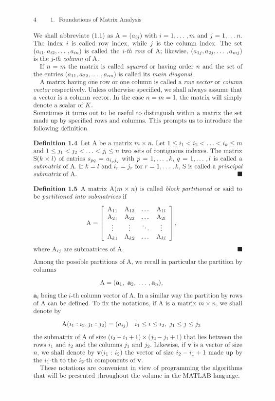
Definition 1.4 Let A be a matrix m% n. Let 1 & i1 < i2 < . . . < ik & mand 1 & j1 < j2 < . . . < jl & n two sets of contiguous indexes. The matrixS(k % l) of entries spq = aipjq with p = 1, . . . , k, q = 1, . . . , l is called asubmatrix of A. If k = l and ir = jr for r = 1, . . . , k, S is called a principalsubmatrix of A. !
Definition 1.5 A matrix A(m % n) is called block partitioned or said tobe partitioned into submatrices if
A =
"
###$
A11 A12 . . . A1lA21 A22 . . . A2l...
.... . .
...Ak1 Ak2 . . . Akl
%
&&&',
where Aij are submatrices of A. !
Among the possible partitions of A, we recall in particular the partition bycolumns
A = (a1, a2, . . . ,an),
ai being the i-th column vector of A. In a similar way the partition by rowsof A can be defined. To fix the notations, if A is a matrix m% n, we shalldenote by
A(i1 : i2, j1 : j2) = (aij) i1 & i & i2, j1 & j & j2
the submatrix of A of size (i2" i1 + 1)% (j2" j1 + 1) that lies between therows i1 and i2 and the columns j1 and j2. Likewise, if v is a vector of sizen, we shall denote by v(i1 : i2) the vector of size i2 " i1 + 1 made up bythe i1-th to the i2-th components of v.
These notations are convenient in view of programming the algorithmsthat will be presented throughout the volume in the MATLAB language.

1.3 Operations with Matrices 5
1.3 Operations with Matrices
Let A = (aij) and B = (bij) be two matrices m % n over K. We say thatA is equal to B, if aij = bij for i = 1, . . . ,m, j = 1, . . . , n. Moreover, wedefine the following operations:
- matrix sum: the matrix sum is the matrix A+B = (aij+bij). The neutralelement in a matrix sum is the null matrix, still denoted by 0 andmade up only by null entries;
- matrix multiplication by a scalar: the multiplication of A by $ ! K, is amatrix $A = ($aij);
- matrix product: the product of two matrices A and B of sizes (m, p)and (p, n) respectively, is a matrix C(m,n) whose entries are cij =p(
k=1
aikbkj , for i = 1, . . . ,m, j = 1, . . . , n.
The matrix product is associative and distributive with respect to the ma-trix sum, but it is not in general commutative. The square matrices forwhich the property AB = BA holds, will be called commutative.
In the case of square matrices, the neutral element in the matrix productis a square matrix of order n called the unit matrix of order n or, morefrequently, the identity matrix given by In = (%ij). The identity matrixis, by definition, the only matrix n % n such that AIn = InA = A for allsquare matrices A. In the following we shall omit the subscript n unless itis strictly necessary. The identity matrix is a special instance of a diagonalmatrix of order n, that is, a square matrix of the type D = (dii%ij). We willuse in the following the notation D = diag(d11, d22, . . . , dnn).Finally, if A is a square matrix of order n and p is an integer, we define Ap
as the product of A with itself iterated p times. We let A0 = I.
Let us now address the so-called elementary row operations that can beperformed on a matrix. They consist of:
- multiplying the i-th row of a matrix by a scalar "; this operation isequivalent to pre-multiplying A by the matrix D = diag(1, . . . , 1,",1, . . . , 1), where " occupies the i-th position;
- exchanging the i-th and j-th rows of a matrix; this can be done by pre-multiplying A by the matrix P(i,j) of elements
p(i,j)rs =
)***+
***,
1 if r = s = 1, . . . , i" 1, i + 1, . . . , j " 1, j + 1, . . . n,
1 if r = j, s = i or r = i, s = j,
0 otherwise,
(1.2)

6 1. Foundations of Matrix Analysis
where Ir denotes the identity matrix of order r = j " i " 1 if j >i (henceforth, matrices with size equal to zero will correspond tothe empty set). Matrices like (1.2) are called elementary permutationmatrices. The product of elementary permutation matrices is calleda permutation matrix, and it performs the row exchanges associatedwith each elementary permutation matrix. In practice, a permutationmatrix is a reordering by rows of the identity matrix;
- adding " times the j-th row of a matrix to its i-th row. This operationcan also be performed by pre-multiplying A by the matrix I + N(i,j)
! ,where N(i,j)
! is a matrix having null entries except the one in positioni, j whose value is ".
1.3.1 Inverse of a MatrixDefinition 1.6 A square matrix A of order n is called invertible (or regularor nonsingular) if there exists a square matrix B of order n such thatA B = B A = I. B is called the inverse matrix of A and is denoted by A"1.A matrix which is not invertible is called singular. !
If A is invertible its inverse is also invertible, with (A"1)"1 = A. Moreover,if A and B are two invertible matrices of order n, their product AB is alsoinvertible, with (A B)"1 = B"1A"1. The following property holds.
Property 1.2 A square matrix is invertible i! its column vectors are lin-early independent.
Definition 1.7 We call the transpose of a matrix A! Rm!n the matrixn%m, denoted by AT , that is obtained by exchanging the rows of A withthe columns of A. !
Clearly, (AT )T = A, (A + B)T = AT + BT , (AB)T = BTAT and ("A)T ="AT #" ! R. If A is invertible, then also (AT )"1 = (A"1)T = A"T .
Definition 1.8 Let A ! Cm!n; the matrix B = AH ! Cn!m is called theconjugate transpose (or adjoint) of A if bij = aji, where aji is the complexconjugate of aji. !
In analogy with the case of the real matrices, it turns out that (A+B)H =AH + BH , (AB)H = BHAH and ("A)H = "AH #" ! C.
Definition 1.9 A matrix A ! Rn!n is called symmetric if A = AT , whileit is antisymmetric if A = "AT . Finally, it is called orthogonal if ATA =AAT = I, that is A"1 = AT . !
Permutation matrices are orthogonal and the same is true for their prod-ucts.
1.3 Operations with Matrices 7
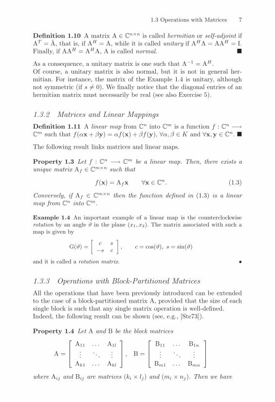
Definition 1.10 A matrix A ! Cn!n is called hermitian or self-adjoint ifAT = A, that is, if AH = A, while it is called unitary if AHA = AAH = I.Finally, if AAH = AHA, A is called normal. !
As a consequence, a unitary matrix is one such that A"1 = AH .Of course, a unitary matrix is also normal, but it is not in general her-mitian. For instance, the matrix of the Example 1.4 is unitary, althoughnot symmetric (if s '= 0). We finally notice that the diagonal entries of anhermitian matrix must necessarily be real (see also Exercise 5).
1.3.2 Matrices and Linear MappingsDefinition 1.11 A linear map from Cn into Cm is a function f : Cn "(Cm such that f("x + #y) = "f(x) + #f(y), #",# ! K and #x,y ! Cn. !
The following result links matrices and linear maps.
Property 1.3 Let f : Cn "( Cm be a linear map. Then, there exists aunique matrix Af ! Cm!n such that
f(x) = Afx #x ! Cn. (1.3)
Conversely, if Af ! Cm!n then the function defined in (1.3) is a linearmap from Cn into Cm.
Example 1.4 An important example of a linear map is the counterclockwiserotation by an angle " in the plane (x1, x2). The matrix associated with such amap is given by
G(") =-
c s%s c
., c = cos("), s = sin(")
and it is called a rotation matrix. •
1.3.3 Operations with Block-Partitioned MatricesAll the operations that have been previously introduced can be extendedto the case of a block-partitioned matrix A, provided that the size of eachsingle block is such that any single matrix operation is well-defined.Indeed, the following result can be shown (see, e.g., [Ste73]).
Property 1.4 Let A and B be the block matrices
A =
"
#$A11 . . . A1l...
. . ....
Ak1 . . . Akl
%
&' , B =
"
#$B11 . . . B1n...
. . ....
Bm1 . . . Bmn
%
&'
where Aij and Bij are matrices (ki % lj) and (mi % nj). Then we have

8 1. Foundations of Matrix Analysis
1.
$A =
"
#$$A11 . . . $A1l
.... . .
...$Ak1 . . . $Akl
%
&' , $ ! C; AT =
"
#$AT
11 . . . ATk1
.... . .
...AT
1l . . . ATkl
%
&' ;
2. if k = m, l = n, mi = ki and nj = lj, then
A + B =
"
#$A11 + B11 . . . A1l + B1l
.... . .
...Ak1 + Bk1 . . . Akl + Bkl
%
&' ;
3. if l = m, li = mi and ki = ni, then, letting Cij =m(
s=1
AisBsj,
AB =
"
#$C11 . . . C1l...
. . ....
Ck1 . . . Ckl
%
&' .
1.4 Trace and Determinant of a Matrix
Let us consider a square matrix A of order n. The trace of a matrix is the
sum of the diagonal entries of A, that is tr(A) =n(
i=1
aii.
We call the determinant of A the scalar defined through the following for-mula
det(A) =(
!#P
sign(!)a1"1a2"2 . . . an"n ,
where P =/! = (&1, . . . ,&n)T
0is the set of the n! vectors that are ob-
tained by permuting the index vector i = (1, . . . , n)T and sign(!) equal to1 (respectively, "1) if an even (respectively, odd) number of exchanges isneeded to obtain ! from i.The following properties hold
det(A) = det(AT ), det(AB) = det(A)det(B), det(A"1) = 1/det(A),
det(AH) = det(A), det("A) = "ndet(A), #" ! K.
Moreover, if two rows or columns of a matrix coincide, the determinantvanishes, while exchanging two rows (or two columns) produces a change

1.5 Rank and Kernel of a Matrix 9
of sign in the determinant. Of course, the determinant of a diagonal matrixis the product of the diagonal entries.
Denoting by Aij the matrix of order n " 1 obtained from A by elimi-nating the i-th row and the j-th column, we call the complementary minorassociated with the entry aij the determinant of the matrix Aij . We callthe k-th principal (dominating) minor of A, dk, the determinant of theprincipal submatrix of order k, Ak = A(1 : k, 1 : k). If we denote by#ij = ("1)i+jdet(Aij) the cofactor of the entry aij , the actual computa-tion of the determinant of A can be performed using the following recursiverelation
det(A) =
)***+
***,
a11 if n = 1,
n(
j=1
#ijaij , for n > 1,(1.4)
which is known as the Laplace rule. If A is a square invertible matrix oforder n, then
A"1 =1
det(A)C
where C is the matrix having entries #ji, i, j = 1, . . . , n.As a consequence, a square matrix is invertible i! its determinant is non-vanishing. In the case of nonsingular diagonal matrices the inverse is stilla diagonal matrix having entries given by the reciprocals of the diagonalentries of the matrix.
Every orthogonal matrix is invertible, its inverse is given by AT , moreoverdet(A) = ±1.
1.5 Rank and Kernel of a Matrix
Let A be a rectangular matrix m % n. We call the determinant of orderq (with q ) 1) extracted from matrix A, the determinant of any squarematrix of order q obtained from A by eliminating m " q rows and n " qcolumns.
Definition 1.12 The rank of A (denoted by rank(A)) is the maximumorder of the nonvanishing determinants extracted from A. A matrix hascomplete or full rank if rank(A) = min(m,n). !
Notice that the rank of A represents the maximum number of linearlyindependent column vectors of A that is, the dimension of the range of A,defined as
range(A) = {y ! Rm : y = Ax for x ! Rn} . (1.5)

10 1. Foundations of Matrix Analysis
Rigorously speaking, one should distinguish between the column rank of Aand the row rank of A, the latter being the maximum number of linearlyindependent row vectors of A. Nevertheless, it can be shown that the rowrank and column rank do actually coincide.
The kernel of A is defined as the subspace
ker(A) = {x ! Rn : Ax = 0} .
The following relations hold
1. rank(A) = rank(AT ) (if A ! Cm!n, rank(A) = rank(AH))
2. rank(A) + dim(ker(A)) = n.
In general, dim(ker(A)) '= dim(ker(AT )). If A is a nonsingular square ma-trix, then rank(A) = n and dim(ker(A)) = 0.
Example 1.5 Let
A =-
1 1 01 %1 1
..
Then, rank(A) = 2, dim(ker(A)) = 1 and dim(ker(AT )) = 0. •
We finally notice that for a matrix A ! Cn!n the following properties areequivalent:
1. A is nonsingular;
2. det(A) '= 0;
3. ker(A) = {0};
4. rank(A) = n;
5. A has linearly independent rows and columns.
1.6 Special Matrices
1.6.1 Block Diagonal MatricesThese are matrices of the form D = diag(D1, . . . ,Dn), where Di are squarematrices with i = 1, . . . , n. Clearly, each single diagonal block can be ofdi!erent size. We shall say that a block diagonal matrix has size n if nis the number of its diagonal blocks. The determinant of a block diagonalmatrix is given by the product of the determinants of the single diagonalblocks.
1.6 Special Matrices 11
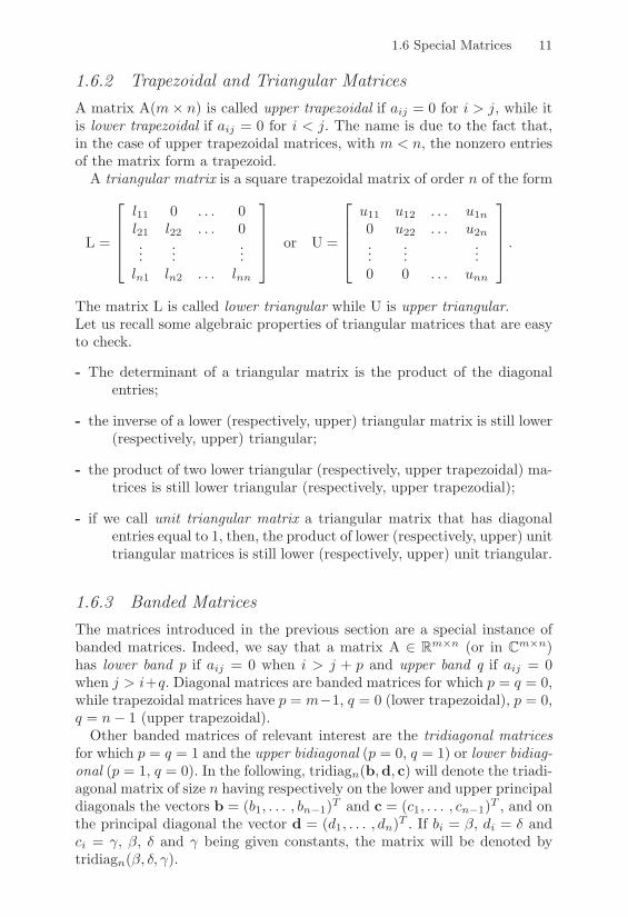
1.6.2 Trapezoidal and Triangular MatricesA matrix A(m% n) is called upper trapezoidal if aij = 0 for i > j, while itis lower trapezoidal if aij = 0 for i < j. The name is due to the fact that,in the case of upper trapezoidal matrices, with m < n, the nonzero entriesof the matrix form a trapezoid.
A triangular matrix is a square trapezoidal matrix of order n of the form
L =
"
###$
l11 0 . . . 0l21 l22 . . . 0...
......
ln1 ln2 . . . lnn
%
&&&'or U =
"
###$
u11 u12 . . . u1n0 u22 . . . u2n...
......
0 0 . . . unn
%
&&&'.
The matrix L is called lower triangular while U is upper triangular.Let us recall some algebraic properties of triangular matrices that are easyto check.
- The determinant of a triangular matrix is the product of the diagonalentries;
- the inverse of a lower (respectively, upper) triangular matrix is still lower(respectively, upper) triangular;
- the product of two lower triangular (respectively, upper trapezoidal) ma-trices is still lower triangular (respectively, upper trapezodial);
- if we call unit triangular matrix a triangular matrix that has diagonalentries equal to 1, then, the product of lower (respectively, upper) unittriangular matrices is still lower (respectively, upper) unit triangular.
1.6.3 Banded MatricesThe matrices introduced in the previous section are a special instance ofbanded matrices. Indeed, we say that a matrix A ! Rm!n (or in Cm!n)has lower band p if aij = 0 when i > j + p and upper band q if aij = 0when j > i+q. Diagonal matrices are banded matrices for which p = q = 0,while trapezoidal matrices have p = m"1, q = 0 (lower trapezoidal), p = 0,q = n" 1 (upper trapezoidal).
Other banded matrices of relevant interest are the tridiagonal matricesfor which p = q = 1 and the upper bidiagonal (p = 0, q = 1) or lower bidiag-onal (p = 1, q = 0). In the following, tridiagn(b,d, c) will denote the triadi-agonal matrix of size n having respectively on the lower and upper principaldiagonals the vectors b = (b1, . . . , bn"1)T and c = (c1, . . . , cn"1)T , and onthe principal diagonal the vector d = (d1, . . . , dn)T . If bi = #, di = % andci = ', #, % and ' being given constants, the matrix will be denoted bytridiagn(#, %, ').

12 1. Foundations of Matrix Analysis
We also mention the so-called lower Hessenberg matrices (p = m " 1,q = 1) and upper Hessenberg matrices (p = 1, q = n " 1) that have thefollowing structure
H =
"
####$
h11 h12 0h21 h22
. . ....
. . . hm"1nhm1 . . . . . . hmn
%
&&&&'or H =
"
####$
h11 h12 . . . h1nh21 h22 h2n
. . . . . ....
0 hmn"1 hmn
%
&&&&'.
Matrices of similar shape can obviously be set up in the block-like format.
1.7 Eigenvalues and Eigenvectors
Let A be a square matrix of order n with real or complex entries; the number$ ! C is called an eigenvalue of A if there exists a nonnull vector x ! Cn
such that Ax = $x. The vector x is the eigenvector associated with theeigenvalue $ and the set of the eigenvalues of A is called the spectrum of A,denoted by ((A). We say that x and y are respectively a right eigenvectorand a left eigenvector of A, associated with the eigenvalue $, if
Ax = $x, yHA = $yH .
The eigenvalue $ corresponding to the eigenvector x can be determined bycomputing the Rayleigh quotient $ = xHAx/(xHx). The number $ is thesolution of the characteristic equation
pA($) = det(A" $I) = 0,
where pA($) is the characteristic polynomial. Since this latter is a polyno-mial of degree n with respect to $, there certainly exist n eigenvalues of Anot necessarily distinct. The following properties can be proved
det(A) =n1
i=1
$i, tr(A) =n(
i=1
$i, (1.6)
and since det(AT "$I) = det((A"$I)T ) = det(A"$I) one concludes that((A) = ((AT ) and, in an analogous way, that ((AH) = ((A).
From the first relation in (1.6) it can be concluded that a matrix issingular i! it has at least one null eigenvalue, since pA(0) = det(A) =$n
i=1$i.Secondly, if A has real entries, pA($) turns out to be a real-coe"cient
polynomial so that complex eigenvalues of A shall necessarily occur in com-plex conjugate pairs.

1.7 Eigenvalues and Eigenvectors 13
Finally, due to the Cayley-Hamilton Theorem if pA($) is the charac-teristic polynomial of A, then pA(A) = 0, where pA(A) denotes a matrixpolynomial (for the proof see, e.g., [Axe94], p. 51).
The maximum module of the eigenvalues of A is called the spectral radiusof A and is denoted by
)(A) = max##$(A)
|$|. (1.7)
Characterizing the eigenvalues of a matrix as the roots of a polynomialimplies in particular that $ is an eigenvalue of A ! Cn!n i! $ is an eigen-value of AH . An immediate consequence is that )(A) = )(AH). Moreover,#A ! Cn!n, #" ! C, )("A) = |"|)(A), and )(Ak) = [)(A)]k #k ! N.
Finally, assume that A is a block triangular matrix
A =
"
###$
A11 A12 . . . A1k0 A22 . . . A2k...
. . ....
0 . . . 0 Akk
%
&&&'.
As pA($) = pA11($)pA22
($) · · · pAkk($), the spectrum of A is given by the
union of the spectra of each single diagonal block. As a consequence, if Ais triangular, the eigenvalues of A are its diagonal entries.
For each eigenvalue $ of a matrix A the set of the eigenvectors associatedwith $, together with the null vector, identifies a subspace of Cn which iscalled the eigenspace associated with $ and corresponds by definition toker(A-$I). The dimension of the eigenspace is
dim [ker(A" $I)] = n" rank(A" $I),
and is called geometric multiplicity of the eigenvalue $. It can never begreater than the algebraic multiplicity of $, which is the multiplicity of$ as a root of the characteristic polynomial. Eigenvalues having geometricmultiplicity strictly less than the algebraic one are called defective. A matrixhaving at least one defective eigenvalue is called defective.
The eigenspace associated with an eigenvalue of a matrix A is invariantwith respect to A in the sense of the following definition.
Definition 1.13 A subspace S in Cn is called invariant with respect to asquare matrix A if AS * S, where AS is the transformed of S through A.!

14 1. Foundations of Matrix Analysis
1.8 Similarity Transformations
Definition 1.14 Let C be a square nonsingular matrix having the sameorder as the matrix A. We say that the matrices A and C"1AC are similar,and the transformation from A to C"1AC is called a similarity transfor-mation. Moreover, we say that the two matrices are unitarily similar if Cis unitary. !Two similar matrices share the same spectrum and the same characteris-tic polynomial. Indeed, it is easy to check that if ($,x) is an eigenvalue-eigenvector pair of A, ($,C"1x) is the same for the matrix C"1AC since
(C"1AC)C"1x = C"1Ax = $C"1x.
We notice in particular that the product matrices AB and BA, with A !Cn!m and B ! Cm!n, are not similar but satisfy the following property(see [Hac94], p.18, Theorem 2.4.6)
((AB)\ {0} = ((BA)\ {0}
that is, AB and BA share the same spectrum apart from null eigenvaluesso that )(AB) = )(BA).
The use of similarity transformations aims at reducing the complexityof the problem of evaluating the eigenvalues of a matrix. Indeed, if a givenmatrix could be transformed into a similar matrix in diagonal or triangularform, the computation of the eigenvalues would be immediate. The mainresult in this direction is the following theorem (for the proof, see [Dem97],Theorem 4.2).
Property 1.5 (Schur decomposition) Given A! Cn!n, there exists Uunitary such that
U"1AU = UHAU =
"
###$
$1 b12 . . . b1n0 $2 b2n...
. . ....
0 . . . 0 $n
%
&&&'= T,
where $i are the eigenvalues of A.
It thus turns out that every matrix A is unitarily similar to an uppertriangular matrix. The matrices T and U are not necessarily unique [Hac94].The Schur decomposition theorem gives rise to several important results;among them, we recall:
1. every hermitian matrix is unitarily similar to a diagonal real ma-trix, that is, when A is hermitian every Schur decomposition of A isdiagonal. In such an event, since
U"1AU = % = diag($1, . . . ,$n),

1.8 Similarity Transformations 15
it turns out that AU = U%, that is, Aui = $iui for i = 1, . . . , n sothat the column vectors of U are the eigenvectors of A. Moreover,since the eigenvectors are orthogonal two by two, it turns out thatan hermitian matrix has a system of orthonormal eigenvectors thatgenerates the whole space Cn. Finally, it can be shown that a matrixA of order n is similar to a diagonal matrix D i! the eigenvectors ofA form a basis for Cn [Axe94];
2. a matrix A ! Cn!n is normal i! it is unitarily similar to a diagonalmatrix. As a consequence, a normal matrix A ! Cn!n admits thefollowing spectral decomposition: A = U%UH =
!ni=1 $iuiuH
i beingU unitary and % diagonal [SS90];
3. let A and B be two normal and commutative matrices; then, thegeneric eigenvalue µi of A+B is given by the sum $i + *i, where$i and *i are the eigenvalues of A and B associated with the sameeigenvector.
There are, of course, nonsymmetric matrices that are similar to diagonalmatrices, but these are not unitarily similar (see, e.g., Exercise 7).
The Schur decomposition can be improved as follows (for the proof see,e.g., [Str80], [God66]).
Property 1.6 (Canonical Jordan Form) Let A be any square matrix.Then, there exists a nonsingular matrix X which transforms A into a blockdiagonal matrix J such that
X"1AX = J = diag (Jk1($1), Jk2($2), . . . , Jkl($l)) ,
which is called canonical Jordan form, $j being the eigenvalues of A andJk($) ! Ck!k a Jordan block of the form J1($) = $ if k = 1 and
Jk($) =
"
#######$
$ 1 0 . . . 0
0 $ 1 · · ·...
.... . . . . . 1 0
.... . . $ 1
0 . . . . . . 0 $
%
&&&&&&&'
, for k > 1.
If an eigenvalue is defective, the size of the corresponding Jordan blockis greater than one. Therefore, the canonical Jordan form tells us that amatrix can be diagonalized by a similarity transformation i! it is nonde-fective. For this reason, the nondefective matrices are called diagonalizable.In particular, normal matrices are diagonalizable.

16 1. Foundations of Matrix Analysis
Partitioning X by columns, X = (x1, . . . ,xn), it can be seen that theki vectors associated with the Jordan block Jki($i) satisfy the followingrecursive relation
Axl = $ixl, l =i"1(
j=1
mj + 1,
Axj = $ixj + xj"1, j = l + 1, . . . , l " 1 + ki, if ki '= 1.
(1.8)
The vectors xi are called principal vectors or generalized eigenvectors of A.
Example 1.6 Let us consider the following matrix
A =
"
######$
7/4 3/4 %1/4 %1/4 %1/4 1/40 2 0 0 0 0
%1/2 %1/2 5/2 1/2 %1/2 1/2%1/2 %1/2 %1/2 5/2 1/2 1/2%1/4 %1/4 %1/4 %1/4 11/4 1/4%3/2 %1/2 %1/2 1/2 1/2 7/2
%
&&&&&&'.
The Jordan canonical form of A and its associated matrix X are given by
J =
"
######$
2 1 0 0 0 00 2 0 0 0 00 0 3 1 0 00 0 0 3 1 00 0 0 0 3 00 0 0 0 0 2
%
&&&&&&', X =
"
######$
1 0 0 0 0 10 1 0 0 0 10 0 1 0 0 10 0 0 1 0 10 0 0 0 1 11 1 1 1 1 1
%
&&&&&&'.
Notice that two di"erent Jordan blocks are related to the same eigenvalue (# =2). It is easy to check property (1.8). Consider, for example, the Jordan blockassociated with the eigenvalue #2 = 3; we have
Ax3 = [0 0 3 0 0 3]T = 3 [0 0 1 0 0 1]T = #2x3,Ax4 = [0 0 1 3 0 4]T = 3 [0 0 0 1 0 1]T + [0 0 1 0 0 1]T = #2x4 + x3,Ax5 = [0 0 0 1 3 4]T = 3 [0 0 0 0 1 1]T + [0 0 0 1 0 1]T = #2x5 + x4.
•
1.9 The Singular Value Decomposition (SVD)
Any matrix can be reduced in diagonal form by a suitable pre and post-multiplication by unitary matrices. Precisely, the following result holds.
Property 1.7 Let A! Cm!n. There exist two unitary matrices U! Cm!m
and V! Cn!n such that
UHAV = & = diag((1, . . . ,(p) ! Cm!n with p = min(m,n) (1.9)
and (1 ) . . . ) (p ) 0. Formula (1.9) is called Singular Value Decompo-sition or (SVD) of A and the numbers (i (or (i(A)) are called singularvalues of A.

1.10 Scalar Product and Norms in Vector Spaces 17
If A is a real-valued matrix, U and V will also be real-valued and in (1.9)UT must be written instead of UH . The following characterization of thesingular values holds
(i(A) =2$i(AHA), i = 1, . . . , n. (1.10)
Indeed, from (1.9) it follows that A = U&VH , AH = V&UH so that, U andV being unitary, AHA = V&2VH , that is, $i(AHA) = $i(&2) = ((i(A))2.Since AAH and AHA are hermitian matrices, the columns of U, called theleft singular vectors of A, turn out to be the eigenvectors of AAH (seeSection 1.8) and, therefore, they are not uniquely defined. The same holdsfor the columns of V, which are the right singular vectors of A.
Relation (1.10) implies that if A ! Cn!n is hermitian with eigenvalues givenby $1, $2, . . . ,$n, then the singular values of A coincide with the modulesof the eigenvalues of A. Indeed because AAH = A2, (i =
3$2i = |$i| for
i = 1, . . . , n. As far as the rank is concerned, if
(1 ) . . . ) (r > (r+1 = . . . = (p = 0,
then the rank of A is r, the kernel of A is the span of the column vectorsof V, {vr+1, . . . ,vn}, and the range of A is the span of the column vectorsof U, {u1, . . . ,ur}.
Definition 1.15 Suppose that A! Cm!n has rank equal to r and that itadmits a SVD of the type UHAV = &. The matrix A† = V&†UH is calledthe Moore-Penrose pseudo-inverse matrix, being
&† = diag4
1(1
, . . . ,1(r
, 0, . . . , 05. (1.11)
!
The matrix A† is also called the generalized inverse of A (see Exercise 13).Indeed, if rank(A) = n < m, then A† = (ATA)"1AT , while if n = m =rank(A), A† = A"1. For further properties of A†, see also Exercise 12.
1.10 Scalar Product and Norms in Vector Spaces
Very often, to quantify errors or measure distances one needs to computethe magnitude of a vector or a matrix. For that purpose we introduce inthis section the concept of a vector norm and, in the following one, of amatrix norm. We refer the reader to [Ste73], [SS90] and [Axe94] for theproofs of the properties that are reported hereafter.
18 1. Foundations of Matrix Analysis
Definition 1.16 A scalar product on a vector space V defined over Kis any map (·, ·) acting from V % V into K which enjoys the followingproperties:
1. it is linear with respect to the vectors of V, that is
('x + $z,y) = '(x,y) + $(z,y), #x, z ! V, #',$ ! K;
2. it is hermitian, that is, (y,x) = (x,y), #x,y ! V ;
3. it is positive definite, that is, (x,x) > 0, #x '= 0 (in other words,(x,x) ) 0, and (x,x) = 0 if and only if x = 0).
!
In the case V = Cn (or Rn), an example is provided by the classical Eu-clidean scalar product given by
(x,y) = yHx =n(
i=1
xiyi,
where z denotes the complex conjugate of z.
Moreover, for any given square matrix A of order n and for any x, y! Cn
the following relation holds
(Ax,y) = (x,AHy). (1.12)
In particular, since for any matrix Q ! Cn!n, (Qx,Qy) = (x,QHQy), onegets
Property 1.8 Unitary matrices preserve the Euclidean scalar product, thatis, (Qx,Qy) = (x,y) for any unitary matrix Q and for any pair of vectorsx and y.
Definition 1.17 Let V be a vector space over K. We say that the map+ · + from V into R is a norm on V if the following axioms are satisfied:
1. (i) +v+ ) 0 #v ! V and (ii) +v+ = 0 if and only if v = 0;
2. +"v+ = |"|+v+ #" ! K, #v ! V (homogeneity property);
3. +v + w+ & +v++ +w+ #v,w ! V (triangular inequality),
where |"| denotes the absolute value of " if K = R, the module of " ifK = C. !

1.10 Scalar Product and Norms in Vector Spaces 19
The pair (V, + · +) is called a normed space. We shall distinguish amongnorms by a suitable subscript at the margin of the double bar symbol. Inthe case the map | · | from V into R enjoys only the properties 1(i), 2 and3 we shall call such a map a seminorm. Finally, we shall call a unit vectorany vector of V having unit norm.An example of a normed space is Rn, equipped for instance by the p-norm(or Holder norm); this latter is defined for a vector x of components {xi}as
+x+p =
6n(
i=1
|xi|p71/p
, for 1 & p <,. (1.13)
Notice that the limit as p goes to infinity of +x+p exists, is finite, and equalsthe maximum module of the components of x. Such a limit defines in turna norm, called the infinity norm (or maximum norm), given by
+x+$ = max1%i%n
|xi|.
When p = 2, from (1.13) the standard definition of Euclidean norm isrecovered
+x+2 = (x,x)1/2 =
6n(
i=1
|xi|271/2
=8xTx
91/2,
for which the following property holds.
Property 1.9 (Cauchy-Schwarz inequality) For any pair x,y ! Rn,
|(x,y)| = |xTy| & +x+2 +y+2, (1.14)
where strict equality holds i! y = "x for some " ! R.
We recall that the scalar product in Rn can be related to the p-normsintroduced over Rn in (1.13) by the Holder inequality
|(x,y)| & +x+p+y+q, with1p
+1q
= 1.
In the case where V is a finite-dimensional space the following propertyholds (for a sketch of the proof, see Exercise 14).
Property 1.10 Any vector norm +·+ defined on V is a continuous functionof its argument, namely, #+ > 0, -C > 0 such that if +x " :x+ & + then| +x+ " +:x+ | & C+, for any x, :x ! V .
New norms can be easily built using the following result.

20 1. Foundations of Matrix Analysis
Property 1.11 Let + · + be a norm of Rn and A ! Rn!n be a matrix withn linearly independent columns. Then, the function + · +A2 acting from Rn
into R defined as
+x+A2 = +Ax+ #x ! Rn,
is a norm of Rn.
Two vectors x, y in V are said to be orthogonal if (x,y) = 0. This statementhas an immediate geometric interpretation when V = R2 since in such acase
(x,y) = +x+2+y+2 cos(,),
where , is the angle between the vectors x and y. As a consequence, if(x,y) = 0 then , is a right angle and the two vectors are orthogonal in thegeometric sense.
Definition 1.18 Two norms + · +p and + · +q on V are equivalent if thereexist two positive constants cpq and Cpq such that
cpq+x+q & +x+p & Cpq+x+q #x ! V.
!
In a finite-dimensional normed space all norms are equivalent. In particular,if V = Rn it can be shown that for the p-norms, with p = 1, 2, and ,, theconstants cpq and Cpq take the value reported in Table 1.1.
cpq q = 1 q = 2 q = ,p = 1 1 1 1p = 2 n"1/2 1 1p = , n"1 n"1/2 1
Cpq q = 1 q = 2 q = ,p = 1 1 n1/2 np = 2 1 1 n1/2
p = , 1 1 1
TABLE 1.1. Equivalence constants for the main norms of Rn
In this book we shall often deal with sequences of vectors and with theirconvergence. For this purpose, we recall that a sequence of vectors
/x(k)0
in a vector space V having finite dimension n, converges to a vector x, andwe write lim
k&$x(k) = x if
limk&$
x(k)i = xi, i = 1, . . . , n (1.15)
where x(k)i and xi are the components of the corresponding vectors with
respect to a basis of V . If V = Rn, due to the uniqueness of the limit of a

1.11 Matrix Norms 21
sequence of real numbers, (1.15) implies also the uniqueness of the limit, ifexisting, of a sequence of vectors.We further notice that in a finite-dimensional space all the norms are topo-logically equivalent in the sense of convergence, namely, given a sequenceof vectors x(k),
|||x(k)|||( 0 . +x(k)+ ( 0 if k (,,
where ||| · ||| and + · + are any two vector norms. As a consequence, we canestablish the following link between norms and limits.
Property 1.12 Let + · + be a norm in a space finite dimensional space V .Then
limk&$
x(k) = x . limk&$
+x" x(k)+ = 0,
where x ! V and/x(k)0 is a sequence of elements of V .
1.11 Matrix Norms
Definition 1.19 A matrix norm is a mapping + ·+ : Rm!n ( R such that:
1. +A+ ) 0 #A ! Rm!n and +A+ = 0 if and only if A = 0;
2. +"A+ = |"|+A+ #" ! R, #A ! Rm!n (homogeneity);
3. +A + B+ & +A++ +B+ #A,B ! Rm!n (triangular inequality).
!
Unless otherwise specified we shall employ the same symbol + ·+, to denotematrix norms and vector norms.
We can better characterize the matrix norms by introducing the conceptsof compatible norm and norm induced by a vector norm.
Definition 1.20 We say that a matrix norm +·+ is compatible or consistentwith a vector norm + · + if
+Ax+ & +A+ +x+, #x ! Rn. (1.16)
More generally, given three norms, all denoted by + · +, albeit defined onRm, Rn and Rm!n, respectively, we say that they are consistent if #x ! Rn,Ax = y ! Rm, A ! Rm!n, we have that +y+ & +A+ +x+. !
In order to single out matrix norms of practical interest, the followingproperty is in general required

22 1. Foundations of Matrix Analysis
Definition 1.21 We say that a matrix norm + · + is sub-multiplicative if#A ! Rn!m, #B ! Rm!q
+AB+ & +A+ +B+. (1.17)
!
This property is not satisfied by any matrix norm. For example (taken from[GL89]), the norm +A+! = max |aij | for i = 1, . . . , n, j = 1, . . . ,m doesnot satisfy (1.17) if applied to the matrices
A = B =-
1 11 1
.,
since 2 = +AB+! > +A+!+B+! = 1.Notice that, given a certain sub-multiplicative matrix norm + · +!, therealways exists a consistent vector norm. For instance, given any fixed vectory '= 0 in Cn, it su"ces to define the consistent vector norm as
+x+ = +xyH+! x ! Cn.
As a consequence, in the case of sub-multiplicative matrix norms it is nolonger necessary to explicitly specify the vector norm with respect to thematrix norm is consistent.
Example 1.7 The norm
&A&F =
;<<=n(
i,j=1
|aij |2 = tr(AAH) (1.18)
is a matrix norm called the Frobenius norm (or Euclidean norm in Cn2) and is
compatible with the Euclidean vector norm & · &2. Indeed,
&Ax&22 =n(
i=1
>>>>>
n(
j=1
aijxj
>>>>>
2
"n(
i=1
6n(
j=1
|aij |2n(
j=1
|xj |27
= &A&2F &x&22.
Notice that for such a norm &In&F ='n. •
In view of the definition of a natural norm, we recall the following theorem.
Theorem 1.1 Let +·+ be a vector norm. The function
+A+ = supx '=0
+Ax++x+ (1.19)
is a matrix norm called induced matrix norm or natural matrix norm.

1.11 Matrix Norms 23
Proof. We start by noticing that (1.19) is equivalent to
&A& = sup"x"=1
&Ax&. (1.20)
Indeed, one can define for any x $= 0 the unit vector u = x/&x&, so that (1.19)becomes
&A& = sup"u"=1
&Au& = &Aw& with &w& = 1.
This being taken as given, let us check that (1.19) (or, equivalently, (1.20)) isactually a norm, making direct use of Definition 1.19.
1. If &Ax& ! 0, then it follows that &A& = sup"x"=1
&Ax& ! 0. Moreover
&A& = supx#=0
&Ax&&x& = 0( &Ax& = 0 )x $= 0
and Ax = 0 )x $= 0 if and only if A=0; therefore &A& = 0 ( A = 0.2. Given a scalar $,
&$A& = sup"x"=1
&$Ax& = |$| sup"x"=1
&Ax& = |$| &A&.
3. Finally, triangular inequality holds. Indeed, by definition of supremum, ifx $= 0 then
&Ax&&x& " &A& * &Ax& " &A&&x&,
so that, taking x with unit norm, one gets
&(A + B)x& " &Ax&+ &Bx& " &A&+ &B&,
from which it follows that &A + B& = sup"x"=1
&(A + B)x& " &A&+ &B&.
!
Relevant instances of induced matrix norms are the so-called p-norms de-fined as
+A+p = supx'=0
+Ax+p+x+p
The 1-norm and the infinity norm are easily computable since
+A+1 = maxj=1,... ,n
m(
i=1
|aij |, +A+$ = maxi=1,... ,m
n(
j=1
|aij |
and they are called the column sum norm and the row sum norm, respec-tively.
Moreover, we have +A+1 = +AT +$ and, if A is self-adjoint or real sym-metric, +A+1 = +A+$.
A special discussion is deserved by the 2-norm or spectral norm for whichthe following theorem holds.
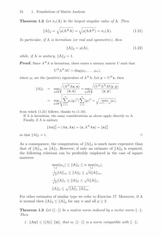
24 1. Foundations of Matrix Analysis
Theorem 1.2 Let (1(A) be the largest singular value of A. Then
+A+2 =2)(AHA) =
2)(AAH) = (1(A). (1.21)
In particular, if A is hermitian (or real and symmetric), then
+A+2 = )(A), (1.22)
while, if A is unitary, +A+2 = 1.
Proof. Since AHA is hermitian, there exists a unitary matrix U such that
UHAHAU = diag(µ1, . . . , µn),
where µi are the (positive) eigenvalues of AHA. Let y = UHx, then
&A&2 = supx#=0
?(AHAx,x)
(x,x)= sup
y #=0
?(UHAHAUy,y)
(y,y)
= supy #=0
;<<=n(
i=1
µi|yi|2/n(
i=1
|yi|2 =2
maxi=1,... ,n
|µi|,
from which (1.21) follows, thanks to (1.10).If A is hermitian, the same considerations as above apply directly to A.Finally, if A is unitary
&Ax&22 = (Ax,Ax) = (x,AHAx) = &x&22
so that &A&2 = 1. !
As a consequence, the computation of +A+2 is much more expensive thanthat of +A+$ or +A+1. However, if only an estimate of +A+2 is required,the following relations can be profitably employed in the case of squarematrices
maxi,j
|aij | & +A+2 & n maxi,j
|aij |,1(n+A+$ & +A+2 &
/n+A+$,
1(n+A+1 & +A+2 &
/n+A+1,
+A+2 &3+A+1 +A+$.
For other estimates of similar type we refer to Exercise 17. Moreover, if Ais normal then +A+2 & +A+p for any n and all p ) 2.
Theorem 1.3 Let ||| · ||| be a matrix norm induced by a vector norm + · +.Then
1. +Ax+ & |||A||| +x+, that is, ||| · ||| is a norm compatible with + · +;

1.11 Matrix Norms 25
2. |||I||| = 1;
3. |||AB||| & |||A||| |||B|||, that is, ||| · ||| is sub-multiplicative.
Proof. Part 1 of the theorem is already contained in the proof of Theorem 1.1,while part 2 follows from the fact that |||I||| = sup
x#=0&Ix&/&x& = 1. Part 3 is simple
to check. !
Notice that the p-norms are sub-multiplicative. Moreover, we remark thatthe sub-multiplicativity property by itself would only allow us to concludethat |||I||| ) 1. Indeed, |||I||| = |||I · I||| & |||I|||2.
1.11.1 Relation between Norms and the Spectral Radius of aMatrix
We next recall some results that relate the spectral radius of a matrix tomatrix norms and that will be widely employed in Chapter 4.
Theorem 1.4 Let + · + be a consistent matrix norm; then
)(A) & +A+ #A ! Cn!n.
Proof. Let # be an eigenvalue of A and v $= 0 an associated eigenvector. As aconsequence, since & · & is consistent, we have
|#| &v& = &#v& = &Av& " &A& &v&
so that |#| " &A&. !
More precisely, the following property holds (see for the proof [IK66], p.12, Theorem 3).
Property 1.13 Let A ! Cn!n and + > 0. Then, there exists a consistentmatrix norm + · +A,% (depending on +) such that
+A+A,% & )(A) + +.
As a result, having fixed an arbitrarily small tolerance, there always existsa matrix norm which is arbitrarily close to the spectral radius of A, namely
)(A) = inf)·)+A+, (1.23)
the infimum being taken on the set of all the consistent norms.For the sake of clarity, we notice that the spectral radius is a sub-
multiplicative seminorm, since it is not true that )(A) = 0 i! A = 0.As an example, any triangular matrix with null diagonal entries clearly hasspectral radius equal to zero. Moreover, we have the following result.

26 1. Foundations of Matrix Analysis
Property 1.14 Let A be a square matrix and let +·+ be a consistent norm.Then
limm&$
+Am+1/m = )(A).
1.11.2 Sequences and Series of MatricesA sequence of matrices
/A(k)0 ! Rn!n is said to converge to a matrix
A ! Rn!n if
limk&$
+A(k) "A+ = 0.
The choice of the norm does not influence the result since in Rn!n all normsare equivalent. In particular, when studying the convergence of iterativemethods for solving linear systems (see Chapter 4), one is interested in theso-called convergent matrices for which
limk&$
Ak = 0,
0 being the null matrix. The following theorem holds.
Theorem 1.5 Let A be a square matrix; then
limk&$
Ak = 0 . )(A) < 1. (1.24)
Moreover, the geometric series$(
k=0
Ak is convergent i! )(A) < 1. In such a
case$(
k=0
Ak = (I"A)"1. (1.25)
As a result, if )(A) < 1 the matrix I " A is invertible and the followinginequalities hold
11 + +A+ & +(I"A)"1+ & 1
1" +A+ (1.26)
where + · + is an induced matrix norm such that +A+ < 1.
Proof. Let us prove (1.24). Let %(A) < 1, then +& > 0 such that %(A) < 1 % &and thus, thanks to Property 1.13, there exists a consistent matrix norm & ·& suchthat &A& " %(A) + & < 1. From the fact that &Ak& " &A&k < 1 and from thedefinition of convergence it turns out that as k , # the sequence
/Ak
0tends
to zero. Conversely, assume that limk$!
Ak = 0 and let # denote an eigenvalue of
A. Then, Akx = #kx, being x( $=0) an eigenvector associated with #, so that

1.12 Positive Definite, Diagonally Dominant and M-matrices 27
limk$!
#k = 0. As a consequence, |#| < 1 and because this is true for a genericeigenvalue one gets %(A) < 1 as desired. Relation (1.25) can be obtained notingfirst that the eigenvalues of I%A are given by 1 % #(A), #(A) being the genericeigenvalue of A. On the other hand, since %(A) < 1, we deduce that I%A isnonsingular. Then, from the identity
(I%A)(I + A + . . . + An) = (I%An+1)
and taking the limit for n tending to infinity the thesis follows since
(I%A)!(
k=0
Ak = I.
Finally, thanks to Theorem 1.3, the equality &I& = 1 holds, so that
1 = &I& " &I%A& &(I%A)%1& " (1 + &A&) &(I%A)%1&,
giving the first inequality in (1.26). As for the second part, noting that I =I%A+A and multiplying both sides on the right by (I%A)%1, one gets (I%A)%1 =I + A(I%A)%1. Passing to the norms, we obtain
&(I%A)%1& " 1 + &A& &(I%A)%1&,
and thus the second inequality, since &A& < 1. !
Remark 1.1 The assumption that there exists an induced matrix normsuch that +A+ < 1 is justified by Property 1.13, recalling that A is conver-gent and, therefore, )(A) < 1. !
Notice that (1.25) suggests an algorithm to approximate the inverse of amatrix by a truncated series expansion.
1.12 Positive Definite, Diagonally Dominant andM-matrices
Definition 1.22 A matrix A ! Cn!n is positive definite in Cn if the num-ber (Ax,x) is real and positive #x ! Cn, x '= 0. A matrix A ! Rn!n ispositive definite in Rn if (Ax,x) > 0 #x ! Rn, x '= 0. If the strict in-equality is substituted by the weak one ()) the matrix is called positivesemidefinite. !
Example 1.8 Matrices that are positive definite in Rn are not necessarily sym-metric. An instance is provided by matrices of the form
A =-
2 $%2% $ 2
.(1.27)

28 1. Foundations of Matrix Analysis
for $ $= %1. Indeed, for any non null vector x = (x1, x2)T in R2
(Ax,x) = 2(x21 + x2
2 % x1x2) > 0.
Notice that A is not positive definite in C2. Indeed, if we take a complex vectorx we find out that the number (Ax,x) is not real-valued in general. •
Definition 1.23 Let A ! Rn!n. The matrices
AS =12(A + AT ), ASS =
12(A"AT )
are respectively called the symmetric part and the skew-symmetric partof A. Obviously, A = AS + ASS . If A ! Cn!n, the definitions modify asfollows: AS = 1
2 (A + AH) and ASS = 12 (A"AH). !
The following property holds
Property 1.15 A real matrix A of order n is positive definite i! its sym-metric part AS is positive definite.
Indeed, it su"ces to notice that, due to (1.12) and the definition of ASS ,xTASSx = 0 #x ! Rn. For instance, the matrix in (1.27) has a positivedefinite symmetric part, since
AS =12(A + AT ) =
-2 "1"1 2
..
This holds more generally (for the proof see [Axe94]).
Property 1.16 Let A ! Cn!n (respectively, A ! Rn!n); if (Ax,x) is real-valued #x ! Cn, then A is hermitian (respectively, symmetric).
An immediate consequence of the above results is that matrices that arepositive definite in Cn do satisfy the following characterizing property.
Property 1.17 A square matrix A of order n is positive definite in Cn
i! it is hermitian and has positive eigenvalues. Thus, a positive definitematrix is nonsingular.
In the case of positive definite real matrices in Rn, results more specificthan those presented so far hold only if the matrix is also symmetric (this isthe reason why many textbooks deal only with symmetric positive definitematrices). In particular
Property 1.18 Let A ! Rn!n be symmetric. Then, A is positive definitei! one of the following properties is satisfied:
1. (Ax,x) > 0 #x '= 0 with x! Rn;
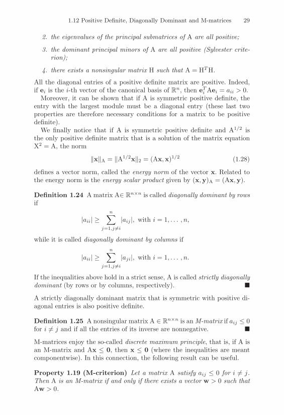
1.12 Positive Definite, Diagonally Dominant and M-matrices 29
2. the eigenvalues of the principal submatrices of A are all positive;
3. the dominant principal minors of A are all positive (Sylvester crite-rion);
4. there exists a nonsingular matrix H such that A = HTH.
All the diagonal entries of a positive definite matrix are positive. Indeed,if ei is the i-th vector of the canonical basis of Rn, then eTi Aei = aii > 0.
Moreover, it can be shown that if A is symmetric positive definite, theentry with the largest module must be a diagonal entry (these last twoproperties are therefore necessary conditions for a matrix to be positivedefinite).
We finally notice that if A is symmetric positive definite and A1/2 isthe only positive definite matrix that is a solution of the matrix equationX2 = A, the norm
+x+A = +A1/2x+2 = (Ax,x)1/2 (1.28)
defines a vector norm, called the energy norm of the vector x. Related tothe energy norm is the energy scalar product given by (x,y)A = (Ax,y).
Definition 1.24 A matrix A! Rn!n is called diagonally dominant by rowsif
|aii| )n(
j=1,j '=i
|aij |, with i = 1, . . . , n,
while it is called diagonally dominant by columns if
|aii| )n(
j=1,j '=i
|aji|, with i = 1, . . . , n.
If the inequalities above hold in a strict sense, A is called strictly diagonallydominant (by rows or by columns, respectively). !
A strictly diagonally dominant matrix that is symmetric with positive di-agonal entries is also positive definite.
Definition 1.25 A nonsingular matrix A ! Rn!n is an M-matrix if aij & 0for i '= j and if all the entries of its inverse are nonnegative. !
M-matrices enjoy the so-called discrete maximum principle, that is, if A isan M-matrix and Ax & 0, then x & 0 (where the inequalities are meantcomponentwise). In this connection, the following result can be useful.
Property 1.19 (M-criterion) Let a matrix A satisfy aij & 0 for i '= j.Then A is an M-matrix if and only if there exists a vector w > 0 such thatAw > 0.
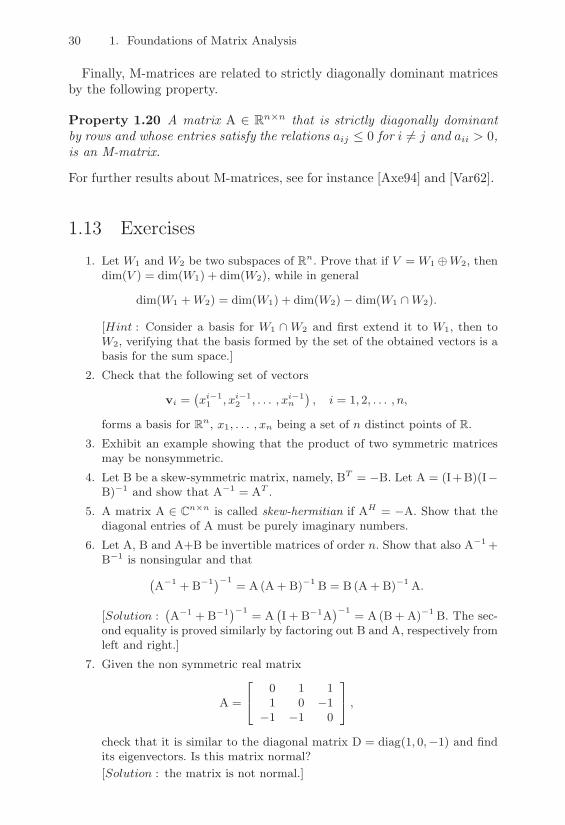
30 1. Foundations of Matrix Analysis
Finally, M-matrices are related to strictly diagonally dominant matricesby the following property.
Property 1.20 A matrix A ! Rn!n that is strictly diagonally dominantby rows and whose entries satisfy the relations aij & 0 for i '= j and aii > 0,is an M-matrix.
For further results about M-matrices, see for instance [Axe94] and [Var62].
1.13 Exercises1. Let W1 and W2 be two subspaces of Rn. Prove that if V = W1 -W2, then
dim(V ) = dim(W1) + dim(W2), while in general
dim(W1 + W2) = dim(W1) + dim(W2)% dim(W1 .W2).
[Hint : Consider a basis for W1 .W2 and first extend it to W1, then toW2, verifying that the basis formed by the set of the obtained vectors is abasis for the sum space.]
2. Check that the following set of vectors
vi =8xi%1
1 , xi%12 , . . . , xi%1
n
9, i = 1, 2, . . . , n,
forms a basis for Rn, x1, . . . , xn being a set of n distinct points of R.
3. Exhibit an example showing that the product of two symmetric matricesmay be nonsymmetric.
4. Let B be a skew-symmetric matrix, namely, BT = %B. Let A = (I+B)(I%B)%1 and show that A%1 = AT .
5. A matrix A / Cn&n is called skew-hermitian if AH = %A. Show that thediagonal entries of A must be purely imaginary numbers.
6. Let A, B and A+B be invertible matrices of order n. Show that also A%1 +B%1 is nonsingular and that
8A%1 + B%19%1 = A(A + B)%1 B = B(A + B)%1 A.
[Solution :8A%1 + B%19%1 = A
8I + B%1A
9%1 = A(B + A)%1 B. The sec-ond equality is proved similarly by factoring out B and A, respectively fromleft and right.]
7. Given the non symmetric real matrix
A =
"
$0 1 11 0 %1
%1 %1 0
%
' ,
check that it is similar to the diagonal matrix D = diag(1, 0,%1) and findits eigenvectors. Is this matrix normal?[Solution : the matrix is not normal.]

1.13 Exercises 31
8. Let A be a square matrix of order n. Check that if P (A) =n(
k=0
ckAk and
#(A) are the eigenvalues of A, then the eigenvalues of P (A) are given by#(P (A)) = P (#(A)). In particular, prove that %(A2) = [%(A)]2.
9. Prove that a matrix of order n having n distinct eigenvalues cannot bedefective. Moreover, prove that a normal matrix cannot be defective.
10. Commutativity of matrix product. Show that if A and B are square matri-ces that share the same set of eigenvectors, then AB = BA. Prove, by acounterexample, that the converse is false.
11. Let A be a normal matrix whose eigenvalues are #1, . . . ,#n. Show that thesingular values of A are |#1|, . . . , |#n|.
12. Let A / Cm&n with rank(A) = n. Show that A† = (ATA)%1AT enjoys thefollowing properties
(1)A†A = In; (2)A†AA† = A†, AA†A = A; (3) if m = n, A† = A%1.
13. Show that the Moore-Penrose pseudo-inverse matrix A† is the only matrixthat minimizes the functional
minX'Cn!m
&AX% Im&F,
where & · &F is the Frobenius norm.
14. Prove Property 1.10.[Solution : For any x, :x / V show that | &x&%&:x& | " &x% :x&. Assumingthat dim(V ) = n and expanding the vector w = x % :x on a basis of V,show that &w& " C&w&!, from which the thesis follows by imposing inthe first obtained inequality that &w&! " &.]
15. Prove Property 1.11 in the case A / Rn&m with m linearly independentcolumns.[Hint : First show that & · &A fulfills all the properties characterizing anorm: positiveness (A has linearly independent columns, thus if x $= 0, thenAx $= 0, which proves the thesis), homogeneity and triangular inequality.]
16. Show that for a rectangular matrix A / Rm&n
&A&2F = '21 + . . . + '2
p,
where p is the minimum between m and n, 'i are the singular values of Aand & · &F is the Frobenius norm.
17. Assuming p, q = 1, 2,#, F , recover the following table of equivalence con-stants cpq such that )A / Rn&n, &A&p " cpq&A&q.
cpq q = 1 q = 2 q =# q = Fp = 1 1
'n n
'n
p = 2'n 1
'n 1
p = # n'n 1
'n
p = F'n
'n
'n 1

32 1. Foundations of Matrix Analysis
18. A matrix norm for which &A& = & |A| & is called absolute norm, havingdenoted by |A| the matrix of the absolute values of the entries of A. Provethat & · &1, & · &! and & · &F are absolute norms, while & · &2 is not. Showthat for this latter
1'n&A&2 " & |A| &2 "
'n&A&2.

2Principles of Numerical Mathematics
The basic concepts of consistency, stability and convergence of a numericalmethod will be introduced in a very general context in the first part ofthe chapter: they provide the common framework for the analysis of anymethod considered henceforth. The second part of the chapter deals withthe computer finite representation of real numbers and the analysis of errorpropagation in machine operations.
2.1 Well-posedness and Condition Number of aProblem
Consider the following problem: find x such that
F (x, d) = 0 (2.1)
where d is the set of data which the solution depends on and F is thefunctional relation between x and d. According to the kind of problemthat is represented in (2.1), the variables x and d may be real numbers,vectors or functions. Typically, (2.1) is called a direct problem if F and dare given and x is the unknown, inverse problem if F and x are knownand d is the unknown, identification problem when x and d are given whilethe functional relation F is the unknown (these latter problems will not becovered in this volume).
Problem (2.1) is well posed if it admits a unique solution x which dependswith continuity on the data. We shall use the terms well posed and stable in

34 2. Principles of Numerical Mathematics
an interchanging manner and we shall deal henceforth only with well-posedproblems.
A problem which does not enjoy the property above is called ill posed orunstable and before undertaking its numerical solution it has to be regular-ized, that is, it must be suitably transformed into a well-posed problem (see,for instance [Mor84]). Indeed, it is not appropriate to pretend the numericalmethod can cure the pathologies of an intrinsically ill-posed problem.
Example 2.1 A simple instance of an ill-posed problem is finding the numberof real roots of a polynomial. For example, the polynomial p(x) = x4 % x2(2a %1) + a(a% 1) exhibits a discontinuous variation of the number of real roots as acontinuously varies in the real field. We have, indeed, 4 real roots if a ! 1, 2 ifa / [0, 1) while no real roots exist if a < 0. •
Continuous dependence on the data means that small perturbations onthe data d yield “small” changes in the solution x. Precisely, denoting by %dan admissible perturbation on the data and by %x the consequent changein the solution, in such a way that
F (x + %x, d + %d) = 0, (2.2)
then
#- > 0, -K(-, d) : +%d+ < - 0 +%x+ & K(-, d)+%d+. (2.3)
The norms used for the data and for the solution may not coincide, when-ever d and x represent variables of di!erent kinds.With the aim of making this analysis more quantitative, we introduce thefollowing definition.
Definition 2.1 For problem (2.1) we define the relative condition numberto be
K(d) = sup&d#D
+%x+/+x++%d+/+d+ , (2.4)
where D is a neighborhood of the origin and denotes the set of admissibleperturbations on the data for which the perturbed problem (2.2) still makessense. Whenever d = 0 or x = 0, it is necessary to introduce the absolutecondition number, given by
Kabs(d) = sup&d#D
+%x++%d+ . (2.5)
!
Problem (2.1) is called ill-conditioned if K(d) is “big” for any admissibledatum d (the precise meaning of “small” and “big” is going to changedepending on the considered problem).

2.1 Well-posedness and Condition Number of a Problem 35
The property of a problem of being well-conditioned is independent ofthe numerical method that is being used to solve it. In fact, it is possibleto generate stable as well as unstable numerical schemes for solving well-conditioned problems. The concept of stability for an algorithm or for anumerical method is analogous to that used for problem (2.1) and will bemade precise in the next section.
Remark 2.1 (Ill-posed problems) Even in the case in which the condi-tion number does not exist (formally, it is infinite), it is not necessarily truethat the problem is ill-posed. In fact there exist well posed problems (forinstance, the search of multiple roots of algebraic equations, see Example2.2) for which the condition number is infinite, but such that they can bereformulated in equivalent problems (that is, having the same solutions)with a finite condition number. !
If problem (2.1) admits a unique solution, then there necessarily exists amapping G, that we call resolvent, between the sets of the data and of thesolutions, such that
x = G(d), that is F (G(d), d) = 0. (2.6)
According to this definition, (2.2) yields x + %x = G(d + %d). Assumingthat G is di!erentiable in d and denoting formally by G*(d) its derivativewith respect to d (if G : Rn ( Rm, G*(d) will be the Jacobian matrix ofG evaluated at the vector d), a Taylor’s expansion of G truncated at firstorder ensures that
G(d + %d)"G(d) = G*(d)%d + o(+%d+) for %d( 0,
where + · + is a suitable norm for %d and o(·) is the classical infinitesimalsymbol denoting an infinitesimal term of higher order with respect to itsargument. Neglecting the infinitesimal of higher order with respect to +%d+,from (2.4) and (2.5) we respectively deduce that
K(d) 1 +G*(d)+ +d++G(d)+ , Kabs(d) 1 +G*(d)+, (2.7)
the symbol + ·+ denoting the matrix norm associated with the vector norm(defined in (1.19)). The estimates in (2.7) are of great practical usefulnessin the analysis of problems in the form (2.6), as shown in the forthcomingexamples.
Example 2.2 (Algebraic equations of second degree) The solutions to thealgebraic equation x2 % 2px + 1 = 0, with p ! 1, are x± = p ±
3p2 % 1. In this
case, F (x, p) = x2%2px+1, the datum d is the coe!cient p, while x is the vectorof components {x+, x%}. As for the condition number, we notice that (2.6) holds

36 2. Principles of Numerical Mathematics
by taking G : R , R2, G(p) = {x+, x%}. Letting G±(p) = x±, it follows thatG(
±(p) = 1 ± p/3
p2 % 1. Using (2.7) with & · & = & · &2 we get
K(p) 0 |p|3p2 % 1
, p > 1. (2.8)
From (2.8) it turns out that in the case of separated roots (say, if p !'
2)problem F (x, p) = 0 is well conditioned. The behavior dramatically changes inthe case of multiple roots, that is when p = 1. First of all, one notices that thefunction G±(p) = p±
3p2 % 1 is no longer di"erentiable for p = 1, which makes
(2.8) meaningless. On the other hand, equation (2.8) shows that, for p close to1, the problem at hand is ill conditioned. However, the problem is not ill posed.Indeed, following Remark 2.1, it is possible to reformulate it in an equivalentmanner as F (x, t) = x2 % ((1 + t2)/t)x + 1 = 0, with t = p +
3p2 % 1, whose
roots x% = t and x+ = 1/t coincide for t = 1. The change of parameter thusremoves the singularity that is present in the former representation of the rootsas functions of p. The two roots x% = x%(t) and x+ = x+(t) are now indeedregular functions of t in the neighborhood of t = 1 and evaluating the conditionnumber by (2.7) yields K(t) 0 1 for any value of t. The transformed problem isthus well conditioned. •
Example 2.3 (Systems of linear equations) Consider the linear system Ax= b, where x and b are two vectors in Rn, while A is the matrix (n1 n) of thereal coe!cients of the system. Suppose that A is nonsingular; in such a case xis the unknown solution x, while the data d are the right-hand side b and thematrix A, that is, d = {bi, aij , 1 " i, j " n}.
Suppose now that we perturb only the right-hand side b. We have d = b,x = G(b) = A%1b so that, G((b) = A%1, and (2.7) yields
K(d) 0 &A%1& &b&&A%1b& =
&Ax&&x& &A
%1& " &A& &A%1& = K(A), (2.9)
where K(A) is the condition number of matrix A (see Section 3.1.1) and the useof a consistent matrix norm is understood. Therefore, if A is well conditioned,solving the linear system Ax=b is a stable problem with respect to perturbationsof the right-hand side b. Stability with respect to perturbations on the entries ofA will be analyzed in Section 3.10. •
Example 2.4 (Nonlinear equations) Let f : R , R be a function of classC1 and consider the nonlinear equation
F (x, d) = f(x) = ((x)% d = 0,
where ( : R , R is a suitable function and d / R a datum (possibly equalto zero). The problem is well defined only if ( is invertible in a neighborhoodof d: in such a case, indeed, x = (%1(d) and the resolvent is G = (%1. Since((%1)((d) = [(((x)]%1, the first relation in (2.7) yields, for d $= 0,
K(d) 0 |d||x| |[(
((x)]%1|, (2.10)

2.2 Stability of Numerical Methods 37
while if d = 0 or x = 0 we have
Kabs(d) 0 |[(((x)]%1|. (2.11)
The problem is thus ill posed if x is a multiple root of ((x)%d; it is ill conditionedwhen (((x) is “small”, well conditioned when (((x) is “large”. We shall furtheraddress this subject in Section 6.1. •
In view of (2.8), the quantity +G*(d)+ is an approximation of Kabs(d) andis sometimes called first order absolute condition number. This latter rep-resents the limit of the Lipschitz constant of G (see Section 11.1) as theperturbation on the data tends to zero.Such a number does not always provide a sound estimate of the conditionnumber Kabs(d). This happens, for instance, when G* vanishes at a pointwhilst G is non null in a neighborhood of the same point. For example,take x = G(d) = cos(d)" 1 for d ! ("&/2,&/2); we have G*(0) = 0, whileKabs(0) = 2/&.
2.2 Stability of Numerical Methods
We shall henceforth suppose the problem (2.1) to be well posed. A numer-ical method for the approximate solution of (2.1) will consist, in general,of a sequence of approximate problems
Fn(xn, dn) = 0 n ) 1 (2.12)
depending on a certain parameter n (to be defined case by case). Theunderstood expectation is that xn ( x as n ( ,, i.e. that the numericalsolution converges to the exact solution. For that, it is necessary that dn (d and that Fn “approximates” F , as n ( ,. Precisely, if the datum d ofproblem (2.1) is admissible for Fn, we say that (2.12) is consistent if
Fn(x, d) = Fn(x, d)" F (x, d) ( 0 for n(, (2.13)
where x is the solution to problem (2.1) corresponding to the datum d.The meaning of this definition will be made precise in the next chapters
for any single class of considered problems.A method is said to be strongly consistent if Fn(x, d) = 0 for any value
of n and not only for n(,.In some cases (e.g., when iterative methods are used) problem (2.12)
could take the following form
Fn(xn, xn"1, . . . , xn"q, dn) = 0 n ) q (2.14)
where x0, x1, . . . , xq"1 are given. In such a case, the property of strongconsistency becomes Fn(x, x, . . . , x, d) = 0 for all n ) q.
38 2. Principles of Numerical Mathematics
Example 2.5 Let us consider the following iterative method (known as New-ton’s method and discussed in Section 6.2.2) for approximating a simple root $of a function f : R , R,
given x0, xn = xn%1 %f(xn%1)f ((xn%1)
, n ! 1. (2.15)
The method (2.15) can be written in the form (2.14) by setting Fn(xn, xn%1, f) =xn % xn%1 + f(xn%1)/f ((xn%1) and is strongly consistent since Fn($,$, f) = 0for all n ! 1.
Consider now the following numerical method (known as the composite mid-point rule discussed in Section 9.2) for approximating x =
@ b
af(t) dt,
xn = Hn(
k=1
f
4tk + tk+1
2
5, n ! 1
where H = (b % a)/n and tk = a + (k % 1)H, k = 1, . . . , (n + 1). This methodis consistent; it is also strongly consistent provided thet f is a piecewise linearpolynomial.
More generally, all numerical methods obtained from the mathematical prob-lem by truncation of limit operations (such as integrals, derivatives, series, . . . )are not strongly consistent. •
Recalling what has been previously stated about problem (2.1), in orderfor the numerical method to be well posed (or stable) we require that for anyfixed n, there exists a unique solution xn corresponding to the datum dn,that the computation of xn as a function of dn is unique and, furthermore,that xn depends continuously on the data, i.e.
#- > 0, -Kn(-, dn) : +%dn+ < - 0 +%xn+ & Kn(-, dn)+%dn+. (2.16)
As done in (2.4), we introduce for each problem in the sequence (2.12) thequantities
Kn(dn) = sup&dn#Dn
+%xn+/+xn++%dn+/+dn+
, Kabs,n(dn) = sup&dn#Dn
+%xn++%dn+
, (2.17)
and then define
Knum(dn) = limk&$
supn+k
Kn(dn), Knumabs (dn) = lim
k&$supn+k
Kabs,n(dn).
We call Knum(dn) the relative asymptotic condition number of the numer-ical method (2.12) and Knum
abs (dn) absolute asymptotic condition number,corresponding to the datum dn.The numerical method is said to be well conditioned if Knum is “small”for any admissible datum dn, ill conditioned otherwise. As in (2.6), let us
2.2 Stability of Numerical Methods 39
consider the case where, for each n, the functional relation (2.1) defines amapping Gn between the sets of the numerical data and the solutions
xn = Gn(dn), that is Fn(Gn(dn), dn) = 0. (2.18)
Assuming that Gn is di!erentiable, we can obtain from (2.17)
Kn(dn) 1 +G*n(dn)+ +dn+
+Gn(dn)+ , Kabs,n(dn) 1 +G*n(dn)+. (2.19)
Example 2.6 (Sum and subtraction) The function f : R2 , R, f(a, b) =a + b, is a linear mapping whose gradient is the vector f ((a, b) = (1, 1)T . Usingthe vector norm & · &1 defined in (1.13) yields K(a, b) 0 (|a|+ |b|)/(|a+ b|), fromwhich it follows that summing two numbers of the same sign is a well conditionedoperation, being K(a, b) 0 1. On the other hand, subtracting two numbers almostequal is ill conditioned, since |a+ b|2 |a|+ |b|. This fact, already pointed out inExample 2.2, leads to the cancellation of significant digits whenever numbers canbe represented using only a finite number of digits (as in floating-point arithmetic,see Section 2.5). •
Example 2.7 Consider again the problem of computing the roots of a polyno-mial of second degree analyzed in Example 2.2. When p > 1 (separated roots),such a problem is well conditioned. However, we generate an unstable algorithmif we evaluate the root x% by the formula x% = p %
3p2 % 1. This formula is
indeed subject to errors due to numerical cancellation of significant digits (seeSection 2.4) that are introduced by the finite arithmetic of the computer. A pos-sible remedy to this trouble consists of computing x+ = p +
3p2 % 1 at first,
then x% = 1/x+. Alternatively, one can solve F (x, p) = x2 % 2px + 1 = 0 usingNewton’s method (proposed in Example 2.5)
xn = xn%1 % (x2n%1 % 2pxn%1 + 1)/(2xn%1 % 2p) = fn(p), n ! 1, x0 given.
Applying (2.19) for p > 1 yields Kn(p) 0 |p|/|xn % p|. To compute Knum(p)we notice that, in the case when the algorithm converges, the solution xn wouldconverge to one of the roots x+ or x%; therefore, |xn % p| ,
3p2 % 1 and thus
Kn(p) , Knum(p) 0 |p|/3
p2 % 1, in perfect agreement with the value (2.8) ofthe condition number of the exact problem.
We can conclude that Newton’s method for the search of simple roots of asecond order algebraic equation is ill conditioned if |p| is very close to 1, while itis well conditioned in the other cases. •
The final goal of numerical approximation is, of course, to build, throughnumerical problems of the type (2.12), solutions xn that “get closer” to thesolution of problem (2.1) as much as n gets larger. This concept is madeprecise in the next definition.
Definition 2.2 The numerical method (2.12) is convergent i!
#+ > 0 -n0(+), -%(n0, +) > 0 :
#n > n0(+), #+%dn+ < %(n0, +) 0 +x(d)" xn(d + %dn)+ & +,(2.20)

40 2. Principles of Numerical Mathematics
where d is an admissible datum for the problem (2.1), x(d) is the corre-sponding solution and xn(d+ %dn) is the solution of the numerical problem(2.12) with datum d + %dn. !
To verify the implication (2.20) it su"ces to check that under the sameassumptions
+x(d + %dn)" xn(d + %dn)+ & +
2. (2.21)
Indeed, thanks to (2.3) we have
+x(d)" xn(d + %dn)+ & +x(d)" x(d + %dn)+
++x(d + %dn)" xn(d + %dn)+ & K(%(n0, +), d)+%dn++ %2 .
Choosing %dn such that K(%(n0, +), d)+%dn+ < %2 , one obtains (2.20).
Measures of the convergence of xn to x are given by the absolute erroror the relative error, respectively defined as
E(xn) = |x" xn|, Erel(xn) =|x" xn|
|x| , (ifx '= 0). (2.22)
In the cases where x and xn are matrix or vector quantities, in additionto the definitions in (2.22) (where the absolute values are substituted bysuitable norms) it is sometimes useful to introduce the error by componentdefined as
Ecrel(xn) = max
i,j
|(x" xn)ij ||xij |
. (2.23)
2.2.1 Relations between Stability and ConvergenceThe concepts of stability and convergence are strongly connected.First of all, if problem (2.1) is well posed, a necessary condition in orderfor the numerical problem (2.12) to be convergent is that it is stable.
Let us thus assume that the method is convergent, and prove that it isstable by finding a bound for +%xn+. We have
+%xn+ = +xn(d + %dn)" xn(d)+ & +xn(d)" x(d)+
+ +x(d)" x(d + %dn)++ +x(d + %dn)" xn(d + %dn)+
& K(%(n0, +), d)+%dn++ +,
(2.24)
having used (2.3) and (2.21) twice. From (2.24) we can conclude that, for nsu"ciently large, +%xn+/+%dn+ can be bounded by a constant of the order

2.3 A priori and a posteriori Analysis 41
of K(%(n0, +), d), so that the method is stable. Thus, we are interested instable numerical methods since only these can be convergent.
The stability of a numerical method becomes a su"cient condition forthe numerical problem (2.12) to converge if this latter is also consistentwith problem (2.1). Indeed, under these assumptions we have
+x(d + %dn)" xn(d + %dn)+ & +x(d + %dn)" x(d)+
+ +x(d)" xn(d)++ +xn(d)" xn(d + %dn)+.
Thanks to (2.3), the first term at right-hand side can be bounded by +%dn+(up to a multiplicative constant independent of %dn). A similar bound holdsfor the third term, due to the stability property (2.16). Finally, concerningthe remaining term, if Fn is di!erentiable with respect to the variable x,an expansion in a Taylor series gives
Fn(x(d), d)" Fn(xn(d), d) =.Fn
.x|(x,d)(x(d)" xn(d)),
for a suitable x “between” x(d) and xn(d). Assuming also that .Fn/.x isinvertible, we get
x(d)" xn(d) =4.Fn
.x
5"1
|(x,d)[Fn(x(d), d)" Fn(xn(d), d)]. (2.25)
On the other hand, replacing Fn(xn(d), d) with F (x(d), d) (since both termsare equal to zero) and passing to the norms, we find
+x(d)" xn(d)+ &
AAAAA
4.Fn
.x
5"1
|(x,d)
AAAAA +Fn(x(d), d)" F (x(d), d)+.
Thanks to (2.13) we can thus conclude that +x(d)"xn(d)+ ( 0 for n(,.The result that has just been proved, although stated in qualitative terms,is a milestone in numerical analysis, known as equivalence theorem (orLax-Richtmyer theorem): “for a consistent numerical method, stability isequivalent to convergence”. A rigorous proof of this theorem is available in[Dah56] for the case of linear Cauchy problems, or in [Lax65] and in [RM67]for linear well-posed initial value problems.
2.3 A priori and a posteriori Analysis
The stability analysis of a numerical method can be carried out followingdi!erent strategies:
1. forward analysis, which provides a bound to the variations +%xn+ onthe solution due to both perturbations in the data and to errors thatare intrinsic to the numerical method;

42 2. Principles of Numerical Mathematics
2. backward analysis, which aims at estimating the perturbations thatshould be “impressed” to the data of a given problem in order toobtain the results actually computed under the assumption of workingin exact arithmetic. Equivalently, given a certain computed solution:xn, backward analysis looks for the perturbations %dn on the datasuch that Fn(:xn, dn + %dn) = 0. Notice that, when performing suchan estimate, no account at all is taken into the way :xn has beenobtained (that is, which method has been employed to generate it).
Forward and backward analyses are two di!erent instances of the socalled a priori analysis. This latter can be applied to investigate not onlythe stability of a numerical method, but also its convergence. In this caseit is referred to as a priori error analysis, which can again be performedusing either a forward or a backward technique.
A priori error analysis is distincted from the so called a posteriori erroranalysis, which aims at producing an estimate of the error on the groundsof quantities that are actually computed by a specific numerical method.Typically, denoting by :xn the computed numerical solution, approximationto the solution x of problem (2.1), the a posteriori error analysis aims atevaluating the error x" :xn as a function of the residual rn = F (:xn, d) bymeans of constants that are called stability factors (see [EEHJ96]).
Example 2.8 For the sake of illustration, consider the problem of finding thezeros $1, . . . ,$n of a polynomial pn(x) =
!nk=0 akx
k of degree n.Denoting by pn(x) =
!nk=0 akx
k a perturbed polynomial whose zeros are $i,forward analysis aims at estimating the error between two corresponding zeros$i and $i, in terms of the variations on the coe!cients ak % ak, k = 0, 1, . . . , n.
On the other hand, let {$i} be the approximate zeros of pn (computed some-how). Backward analysis provides an estimate of the perturbations !ak whichshould be impressed to the coe!cients so that
!nk=0(ak + !ak)$k
i = 0, for a fixed$i. The goal of a posteriori error analysis would rather be to provide an estimateof the error $i % $i as a function of the residual value pn($i).
This analysis will be carried out in Section 6.1. •
Example 2.9 Consider the linear system Ax=b, where A/ Rn&n is a nonsin-gular matrix.
For the perturbed system Ax = b, forward analysis provides an estimate ofthe error x% x in terms of A% A and b% b, while backward analysis estimatesthe perturbations !A = (!aij) and !b = (!bi) which should be impressed to theentries of A and b in order to get (A + !A):xn = b+ !b, :xn being the solution ofthe linear system (computed somehow). Finally, a posteriori error analysis looksfor an estimate of the error x% :xn as a function of the residual rn = b%A:xn.
We will develop this analysis in Section 3.1. •
It is important to point out the role played by the a posteriori analysis indevising strategies for adaptive error control. These strategies, by suitablychanging the discretization parameters (for instance, the spacing between

2.4 Sources of Error in Computational Models 43
nodes in the numerical integration of a function or a di!erential equation),employ the a posteriori analysis in order to ensure that the error does notexceed a fixed tolerance.
A numerical method that makes use of an adaptive error control is calledadaptive numerical method. In practice, a method of this kind applies in thecomputational process the idea of feedback, by activating on the grounds ofa computed solution a convergence test which ensures the control of errorwithin a fixed tolerance. In case the convergence test fails, a suitable strat-egy for modifying the discretization parameters is automatically adoptedin order to enhance the accuracy of the solution to be newly computed,and the overall procedure is iterated until the convergence check is passed.
2.4 Sources of Error in Computational Models
Whenever the numerical problem (2.12) is an approximation to the math-ematical problem (2.1) and this latter is in turn a model of a physicalproblem (which will be shortly denoted by PP), we shall say that (2.12) isa computational model for PP.
In this process the global error, denoted by e, is expressed by the dif-ference between the actually computed solution, :xn, and the physical so-lution, xph, of which x provides a model. The global error e can thus beinterpreted as being the sum of the error em of the mathematical model,given by x"xph, and the error ec of the computational model, :xn"x, thatis e = em + ec (see Figure 2.1).
PP : xph
F (x, d) = 0
Fn(xn, dn) = 0
em
:xn
e
ea
ec
en
FIGURE 2.1. Errors in computational models
The error em will in turn take into account the error of the mathematicalmodel in strict sense (that is, the extent at which the functional equation(2.1) does realistically describe the problem PP) and the error on the data(that is, how much accurately does d provide a measure of the real physical
44 2. Principles of Numerical Mathematics
data). In the same way, ec turns out to be the combination of the numericaldiscretization error en = xn " x, the error ea introduced by the numericalalgorithm and the roundo! error introduced by the computer during theactual solution of problem (2.12) (see Section 2.5).
In general, we can thus outline the following sources of error:
1. errors due to the model, that can be controlled by a proper choice ofthe mathematical model;
2. errors in the data, that can be reduced by enhancing the accuracy inthe measurement of the data themselves;
3. truncation errors, arising from having replaced in the numerical modellimits by operations that involve a finite number of steps;
4. rounding errors.
The errors at the items 3. and 4. give rise to the computational error. Anumerical method will thus be convergent if this error can be made arbi-trarily small by increasing the computational e!ort. Of course, convergenceis the primary, albeit not unique, goal of a numerical method, the othersbeing accuracy, reliability and e"ciency.
Accuracy means that the errors are small with respect to a fixed tol-erance. It is usually quantified by the order of infinitesimal of the erroren with respect to the discretization characteristic parameter (for instancethe largest grid spacing between the discretization nodes). By the way, wenotice that machine precision does not limit, on theoretical grounds, theaccuracy.
Reliability means it is likely that the global error can be guaranteed to bebelow a certain tolerance. Of course, a numerical model can be consideredto be reliable only if suitably tested, that is, successfully applied to severaltest cases.
E"ciency means that the computational complexity that is needed tocontrol the error (that is, the amount of operations and the size of thememory required) is as small as possible.
Having encountered the term algorithm several times in this section, wecannot refrain from providing an intuitive description of it. By algorithmwe mean a directive that indicates, through elementary operations, all thepassages that are needed to solve a specific problem. An algorithm can inturn contain sub-algorithms and must have the feature of terminating aftera finite number of elementary operations. As a consequence, the executorof the algorithm (machine or human being) must find within the algorithmitself all the instructions to completely solve the problem at hand (providedthat the necessary resources for its execution are available).
For instance, the statement that a polynomial of second degree surelyadmits two roots in the complex plane does not characterize an algorithm,

2.5 Machine Representation of Numbers 45
whereas the formula yielding the roots is an algorithm (provided that thesub-algorithms needed to correctly execute all the operations have beendefined in turn).
Finally, the complexity of an algorithm is a measure of its executingtime. Calculating the complexity of an algorithm is therefore a part of theanalysis of the e"ciency of a numerical method. Since several algorithms,with di!erent complexities, can be employed to solve the same problem P ,it is useful to introduce the concept of complexity of a problem, this lattermeaning the complexity of the algorithm that has minimum complexityamong those solving P . The complexity of a problem is typically measuredby a parameter directly associated with P . For instance, in the case ofthe product of two square matrices, the computational complexity can beexpressed as a function of a power of the matrix size n (see, [Str69]).
2.5 Machine Representation of Numbers
Any machine operation is a!ected by rounding errors or roundo!. They aredue to the fact that on a computer only a finite subset of the set of realnumbers can be represented. In this section, after recalling the positionalnotation of real numbers, we introduce their machine representation.
2.5.1 The Positional SystemLet a base # ! N be fixed with # ) 2, and let x be a real number witha finite number of digits xk with 0 & xk < # for k = "m, . . . , n. Thenotation (conventionally adopted)
x' = ("1)s [xnxn"1 . . . x1x0.x"1x"2 . . . x"m] , xn '= 0 (2.26)
is called the positional representation of x with respect to the base #. Thepoint between x0 and x"1 is called decimal point if the base is 10, binarypoint if the base is 2, while s depends on the sign of x (s = 0 if x is positive,1 if negative). Relation (2.26) actually means
x' = ("1)s6
n(
k="m
xk#k
7
.
Example 2.10 The conventional writing x10 = 425.33 denotes the number x =4 · 102 + 2 · 10 + 5 + 3 · 10%1 + 3 · 10%2, while x6 = 425.33 would denote thereal number x = 4 · 62 + 2 · 6 + 5 + 3 · 6%1 + 3 · 6%2. A rational number can ofcourse have a finite number of digits in a base and an infinite number of digits inanother base. For example, the fraction 1/3 has infinite digits in base 10, beingx10 = 0.3, while it has only one digit in base 3, being x3 = 0.1. •

46 2. Principles of Numerical Mathematics
Any real number can be approximated by numbers having a finite repre-sentation. Indeed, having fixed the base #, the following property holds
#+ > 0, #x' ! R, -y' ! R such that |y' " x' | < +,
where y' has finite positional representation.In fact, given the positive number x' = xnxn"1 . . . x0.x"1 . . . x"m . . . witha number of digits, finite or infinite, for any r ) 1 one can build twonumbers
x(l)' =
r"1(
k=0
xn"k#n"k, x(u)
' = x(l)' + #n"r+1,
having r digits, such that x(l)' < x' < x(u)
' and x(u)' " x(l)
' = #n"r+1. Ifr is chosen in such a way that #n"r+1 < /, then taking y' equal to x(l)
'
or x(u)' yields the desired inequality. This result legitimates the computer
representation of real numbers (and thus by a finite number of digits).
Although theoretically speaking all the bases are equivalent, in the com-putational practice three are the bases generally employed: base 2 or binary,base 10 or decimal (the most natural) and base 16 or hexadecimal. Almostall modern computers use base 2, apart from a few which traditionallyemploy base 16. In what follows, we will assume that # is an even integer.
In the binary representation, digits reduce to the two symbols 0 and 1,called bits (binary digits), while in the hexadecimal case the symbols usedfor the representation of the digits are 0,1,...,9,A,B,C,D,E,F. Clearly,the smaller the adopted base, the longer the string of characters needed torepresent the same number.
To simplify notations, we shall write x instead of x' , leaving the base #understood.
2.5.2 The Floating-point Number SystemAssume a given computer has N memory positions in which to store anynumber. The most natural way to make use of these positions in the rep-resentation of a real number x di!erent from zero is to fix one of them forits sign, N " k " 1 for the integer digits and k for the digits beyond thepoint, in such a way that
x = ("1)s · [aN"2aN"3 . . . ak . ak"1 . . . a0] (2.27)
s being equal to 1 or 0. Notice that one memory position is equivalent toone bit storage only when # = 2. The set of numbers of this kind is calledfixed-point system. Equation (2.27) stands for
x = ("1)s · #"kN"2(
j=0
aj#j (2.28)

2.5 Machine Representation of Numbers 47
and therefore this representation amounts to fixing a scaling factor for allthe representable numbers.The use of fixed point strongly limits the value of the minimum and maxi-mum numbers that can be represented on the computer, unless a very largenumber N of memory positions is employed. This drawback can be easilyovercome if the scaling in (2.28) is allowed to be varying. In such a case,given a non vanishing real number x, its floating-point representation isgiven by
x = ("1)s · (0.a1a2 . . . at) · #e = ("1)s ·m · #e"t (2.29)
where t ! N is the number of allowed significant digits ai (with 0 & ai &# " 1), m = a1a2 . . . at an integer number called mantissa such that 0 &m & #t"1 and e an integer number called exponent. Clearly, the exponentcan vary within a finite interval of admissible values: we let L & e & U(typically L < 0 and U > 0). The N memory positions are now distributedamong the sign (one position), the significant digits (t positions) and thedigits for the exponent (the remaining N " t " 1 positions). The numberzero has a separate representation.
Typically, on the computer there are two formats available for the floating-point number representation: single and double precision. In the case of bi-nary representation, these formats correspond in the standard version tothe representation with N = 32 bits (single precision)
1s
8 bits
e23 bits
m
and with N = 64 bits (double precision)
1s
11 bits
e52 bits
m
Let us denote by
F(#, t, L, U) = {0} 2B
x ! R : x = ("1)s#et(
i=1
ai#"i
C
the set of floating-point numbers with t significant digits, base # ) 2, 0 &ai & # " 1, and range (L,U) with L & e & U .
In order to enforce uniqueness in a number representation, it is typi-cally assumed that a1 '= 0 and m ) #t"1. In such an event a1 is calledthe principal significant digit, while at is the last significant digit and therepresentation of x is called normalized. The mantissa m is now varyingbetween #t"1 and #t " 1.For instance, in the case # = 10, t = 4, L = "1 and U = 4, withoutthe assumption that a1 '= 0, the number 1 would admit the followingrepresentations
0.1000 · 101, 0.0100 · 102, 0.0010 · 103, 0.0001 · 104.

48 2. Principles of Numerical Mathematics
To always have uniqueness in the representation, it is assumed that alsothe number zero has its own sign (typically s = 0 is assumed).It can be immediately noticed that if x ! F(#, t, L, U) then also "x !F(#, t, L, U). Moreover, the following lower and upper bounds hold for theabsolute value of x
xmin = #L"1 & |x| & #U (1" #"t) = xmax. (2.30)
The cardinality of F(#, t, L, U) (henceforth shortly denoted by F) is
card F = 2(# " 1)#t"1(U " L + 1) + 1.
From (2.30) it turns out that it is not possible to represent any number(apart from zero) whose absolute value is less than xmin. This latter limi-tation can be overcome by completing F by the set FD of the floating-pointde-normalized numbers obtained by removing the assumption that a1 isnon null, only for the numbers that are referred to the minimum exponentL. In such a way the uniqueness in the representation is not lost and it ispossible to generate numbers that have mantissa between 1 and #t"1 " 1and belong to the interval ("#L"1,#L"1). The smallest number in this sethas absolute value equal to #L"t.
Example 2.11 The positive numbers in the set F(2, 3,%1, 2) are
(0.111) · 22 =72, (0.110) · 22 = 3, (0.101) · 22 =
52, (0.100) · 22 = 2,
(0.111) · 2 =74, (0.110) · 2 =
32, (0.101) · 2 =
54, (0.100) · 2 = 1,
(0.111) =78, (0.110) =
34, (0.101) =
58, (0.100) =
12,
(0.111) · 2%1 =716
, (0.110) · 2%1 =38, (0.101) · 2%1 =
516
, (0.100) · 2%1 =14.
They are included between xmin = )L%1 = 2%2 = 1/4 and xmax = )U (1%)%t) =22(1%2%3) = 7/2. As a whole, we have ()%1))t%1(U %L+1) = (2%1)23%1(2+1 + 1) = 16 strictly positive numbers. Their opposites must be added to them,as well as the number zero. We notice that when ) = 2, the first significant digitin the normalized representation is necessarily equal to 1 and thus it may not bestored in the computer (in such an event, we call it hidden bit).
When considering also the positive de-normalized numbers, we should completethe above set by adding the following numbers
(.011)2 · 2%1 =316
, (.010)2 · 2%1 =18, (.001)2 · 2%1 =
116
.
According to what previously stated, the smallest de-normalized number is )L%t =2%1%3 = 1/16. •

2.5 Machine Representation of Numbers 49
2.5.3 Distribution of Floating-point NumbersThe floating-point numbers are not equally spaced along the real line, butthey get dense close to the smallest representable number. It can be checkedthat the spacing between a number x ! F and its next nearest y ! F, whereboth x and y are assumed to be non null, is at least #"1/M |x| and at most/M |x|, being /M = #1"t the machine epsilon. This latter represents thedistance between the number 1 and the nearest floating-point number, andtherefore it is the smallest number of F such that 1 + /M > 1.Having instead fixed an interval of the form [#e,#e+1], the numbers of F
that belong to such an interval are equally spaced and have distance equalto #e"t. Decreasing (or increasing) by one the exponent gives rise to adecrement (or increment) of a factor # of the distance between consecutivenumbers.
Unlike the absolute distance, the relative distance between two consecu-tive numbers has a periodic behavior which depends only on the mantissam. Indeed, denoting by ("1)sm(x)#e"t one of the two numbers, the dis-tance #x from the successive one is equal to ("1)s#e"t, which implies thatthe relative distance is
#x
x=
("1)s#e"t
("1)sm(x)#e"t=
1m(x)
. (2.31)
Within the interval [#e,#e+1], the ratio in (2.31) is decreasing as x increasessince in the normalized representation the mantissa varies from #t"1 to #t"1 (not included). However, as soon as x = #e+1, the relative distance getsback to the value #"t+1 and starts decreasing on the successive intervals,as shown in Figure 2.2. This oscillatory phenomenon is called wobblingprecision and the greater the base #, the more pronounced the e!ect. Thisis another reason why small bases are preferably employed in computers.
2.5.4 IEC/IEEE ArithmeticThe possibility of building sets of floating-point numbers that di!er in base,number of significant digits and range of the exponent has prompted in thepast the development, for almost any computer, of a particular system F. Inorder to avoid this proliferation of numerical systems, a standard has beenfixed that is nowadays almost universally accepted. This standard was de-veloped in 1985 by the Institute of Electrical and Electronics Engineers(shortly, IEEE) and was approved in 1989 by the International Electroni-cal Commission (IEC) as the international standard IEC559 and it is nowknown by this name (IEC is an organization analogue to the InternationalStandardization Organization (ISO) in the field of electronics). The stan-dard IEC559 endorses two formats for the floating-point numbers: a basicformat, made by the system F(2, 24,"125, 128) for the single precision,and by F(2, 53,"1021, 1024) for the double precision, both including the

50 2. Principles of Numerical Mathematics
2-126
2-125
2-124
2-123
2
2
-24
-23
FIGURE 2.2. Variation of relative distance for the set of numbersF(2, 24,%125, 128) IEC/IEEE in single precision
de-normalized numbers, and an extended format, for which only the mainlimitations are fixed (see Table 2.1).
single double single doubleN ) 43 bits ) 79 bits t ) 32 ) 64L & "1021 & 16381 U ) 1024 ) 16384
TABLE 2.1. Lower or upper limits in the standard IEC559 for the extendedformat of floating-point numbers
Almost all the computers nowadays satisfy the requirements above. Wesummarize in Table 2.2 the special codings that are used in IEC559 todeal with the values ±0, ±, and with the so-called non numbers (shortly,NaN , that is not a number), which correspond for instance to 0/0 or toother exceptional operations.
value exponent mantissa±0 L" 1 0±, U + 1 0NaN U + 1 '= 0
TABLE 2.2. IEC559 codings of some exceptional values
2.5.5 Rounding of a Real Number in its MachineRepresentation
The fact that on any computer only a subset F(#, t, L, U) of R is actuallyavailable poses several practical problems, first of all the representation in F
2.5 Machine Representation of Numbers 51
of any given real number. To this concern, notice that, even if x and y weretwo numbers in F, the result of an operation on them does not necessarilybelong to F. Therefore, we must define an arithmetic also on F.
The simplest approach to solve the first problem consists of roundingx ! R in such a way that the rounded number belongs to F. Among allthe possible rounding operations, let us consider the following one. Givenx ! R in the normalized positional notation (2.29) let us substitute x byits representant fl(x) in F, defined as
fl(x) = ("1)s(0. a1a2 . . .Dat) · #e, at =E
at if at+1 < #/2at + 1 if at+1 ) #/2. (2.32)
The mapping fl : R ( F is the most commonly used and is called rounding(in the chopping one would take more trivially Dat = at). Clearly, fl(x) = xif x ! F and moreover fl(x) & fl(y) if x & y #x, y ! R (monotonicityproperty).
Remark 2.2 (Overflow and underflow) Everything written so far holdsonly for the numbers that in (2.29) have exponent e within the range of F.If, indeed, x ! (",,"xmax) 2 (xmax,,) the value fl(x) is not defined,while if x ! ("xmin, xmin) the operation of rounding is defined anyway(even in absence of de-normalized numbers). In the first case, if x is theresult of an operation on numbers of F, we speak about overflow, in thesecond case about underflow (or graceful underflow if de-normalized num-bers are accounted for). The overflow is handled by the system through aninterrupt of the executing program. !
Apart from exceptional situations, we can easily quantify the error, ab-solute and relative, that is made by substituting fl(x) for x. The followingresult can be shown (see for instance [Hig96], Theorem 2.2).
Property 2.1 If x ! R is such that xmin & |x| & xmax, then
fl(x) = x(1 + %) with |%| & u (2.33)
where
u =12#1"t =
12/M (2.34)
is the so-called roundo! unit (or machine precision).
As a consequence of (2.33), the following bound holds for the relative error
Erel(x) =|x" fl(x)|
|x| & u, (2.35)
while, for the absolute error, one gets
E(x) = |x" fl(x)| & #e"t|(a1 . . . at.at+1 . . . )" (a1 . . . at)|.

52 2. Principles of Numerical Mathematics
From (2.32), it follows that
|(a1 . . . at.at+1 . . . )" (a1 . . . at)| & #"1 #
2,
from which
E(x) & 12#"t+e.
Remark 2.3 In the MATLAB environment it is possible to know imme-diately the value of /M , which is given by the system variable eps. !
2.5.6 Machine Floating-point OperationsAs previously stated, it is necessary to define on the set of machine numbersan arithmetic which is analogous, as far as possible, to the arithmetic in R.Thus, given any arithmetic operation 3 : R % R ( R on two operands inR (the symbol 3 may denote sum, subtraction, multiplication or division),we shall denote by 3 the corresponding machine operation
3 : R% R ( F, x 3 y = fl(fl(x) 3 fl(y)).
From the properties of floating-point numbers one could expect that for theoperations on two operands, whenever well defined, the following propertyholds: #x, y ! F, -% ! R such that
x 3 y = (x 3 y)(1 + %) with |%| & u. (2.36)
In order for (2.36) to be satisfied when 3 is the operator of subtraction, itwill require an additional assumption on the structure of the numbers in F,that is the presence of the so-called round digit (which is addressed at theend of this section). In particular, when 3 is the sum operator, it followsthat for all x, y ! F (see Exercise 11)
|x + y " (x + y)||x + y| & u(1 + u)
|x| + |y||x + y| + u, (2.37)
so that the relative error associated with every machine operation will besmall, unless x+ y is not small by itself. An aside comment is deserved bythe case of the sum of two numbers close in module, but opposite in sign.In fact, in such a case x+y can be quite small, this generating the so-calledcancellation errors (as evidenced in Example 2.6).
It is important to notice that, together with properties of standard arith-metic that are preserved when passing to floating-point arithmetic (like, forinstance, the commutativity of the sum of two addends, or the product of
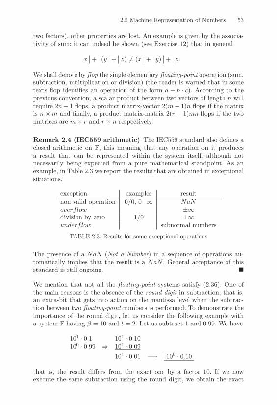
2.5 Machine Representation of Numbers 53
two factors), other properties are lost. An example is given by the associa-tivity of sum: it can indeed be shown (see Exercise 12) that in general
x + (y + z) '= (x + y) + z.
We shall denote by flop the single elementary floating-point operation (sum,subtraction, multiplication or division) (the reader is warned that in sometexts flop identifies an operation of the form a + b · c). According to theprevious convention, a scalar product between two vectors of length n willrequire 2n" 1 flops, a product matrix-vector 2(m" 1)n flops if the matrixis n %m and finally, a product matrix-matrix 2(r " 1)mn flops if the twomatrices are m% r and r % n respectively.
Remark 2.4 (IEC559 arithmetic) The IEC559 standard also defines aclosed arithmetic on F, this meaning that any operation on it producesa result that can be represented within the system itself, although notnecessarily being expected from a pure mathematical standpoint. As anexample, in Table 2.3 we report the results that are obtained in exceptionalsituations.
exception examples resultnon valid operation 0/0, 0 ·, NaNoverflow ±,division by zero 1/0 ±,underflow subnormal numbers
TABLE 2.3. Results for some exceptional operations
The presence of a NaN (Not a Number) in a sequence of operations au-tomatically implies that the result is a NaN . General acceptance of thisstandard is still ongoing. !
We mention that not all the floating-point systems satisfy (2.36). One ofthe main reasons is the absence of the round digit in subtraction, that is,an extra-bit that gets into action on the mantissa level when the subtrac-tion between two floating-point numbers is performed. To demonstrate theimportance of the round digit, let us consider the following example witha system F having # = 10 and t = 2. Let us subtract 1 and 0.99. We have
101 · 0.1 101 · 0.10100 · 0.99 0 101 · 0.09
101 · 0.01 "( 100 · 0.10
that is, the result di!ers from the exact one by a factor 10. If we nowexecute the same subtraction using the round digit, we obtain the exact
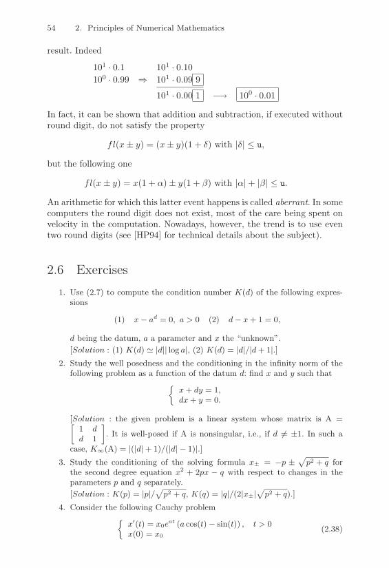
54 2. Principles of Numerical Mathematics
result. Indeed
101 · 0.1 101 · 0.10100 · 0.99 0 101 · 0.09 9
101 · 0.00 1 "( 100 · 0.01
In fact, it can be shown that addition and subtraction, if executed withoutround digit, do not satisfy the property
fl(x± y) = (x± y)(1 + %) with |%| & u,
but the following one
fl(x± y) = x(1 + ") ± y(1 + #) with |"| + |#| & u.
An arithmetic for which this latter event happens is called aberrant. In somecomputers the round digit does not exist, most of the care being spent onvelocity in the computation. Nowadays, however, the trend is to use eventwo round digits (see [HP94] for technical details about the subject).
2.6 Exercises1. Use (2.7) to compute the condition number K(d) of the following expres-
sions
(1) x% ad = 0, a > 0 (2) d% x + 1 = 0,
d being the datum, a a parameter and x the “unknown”.[Solution : (1) K(d) 0 |d|| log a|, (2) K(d) = |d|/|d + 1|.]
2. Study the well posedness and the conditioning in the infinity norm of thefollowing problem as a function of the datum d: find x and y such that
Ex + dy = 1,dx + y = 0.
[Solution : the given problem is a linear system whose matrix is A =-1 dd 1
.. It is well-posed if A is nonsingular, i.e., if d $= ±1. In such a
case, K!(A) = |(|d| + 1)/(|d|% 1)|.]3. Study the conditioning of the solving formula x± = %p ±
3p2 + q for
the second degree equation x2 + 2px % q with respect to changes in theparameters p and q separately.[Solution : K(p) = |p|/
3p2 + q, K(q) = |q|/(2|x±|
3p2 + q).]
4. Consider the following Cauchy problemE
x((t) = x0eat (a cos(t)% sin(t)) , t > 0
x(0) = x0(2.38)

2.6 Exercises 55
whose solution is x(t) = x0eat cos(t) (a is a given real number). Study the
conditioning of (2.38) with respect to the choice of the initial datum andcheck that on unbounded intervals it is well conditioned if a < 0, while itis ill conditioned if a > 0.[Hint : consider the definition of Kabs(a).]
5. Let :x $= 0 be an approximation of a non null quantity x. Find the relationbetween the relative error * = |x% :x|/|x| and E = |x% :x|/|:x|.
6. Find a stable formula for evaluating the square root of a complex number.7. Determine all the elements of the set F = (10, 6,%9, 9), in both normalized
and de-normalized cases.8. Consider the set of the de-normalized numbers FD and study the behavior
of the absolute distance and of the relative distance between two of thesenumbers. Does the wobbling precision e"ect arise again?[Hint : for these numbers, uniformity in the relative density is lost. As aconsequence, the absolute distance remains constant (equal to )L%t), whilethe relative one rapidly grows as x tends to zero.]
9. What is the value of 00 in IEEE arithmetic?[Solution : ideally, the outcome should be NaN . In practice, IEEE systemsrecover the value 1. A motivation of this result can be found in [Gol91].]
10. Show that, due to cancellation errors, the following sequence
I0 = log65, Ik + 5Ik%1 =
1k, k = 1, 2, . . . , n, (2.39)
is not well suited to finite arithmetic computations of the integral In =@ 10
xn
x + 5dx when n is su!ciently large, although it works in infinite arith-
metic.[Hint : consider the initial perturbed datum I0 = I0 + µ0 and study thepropagation of the error µ0 within (2.39).]
11. Prove (2.37).[Solution : notice that
|x + y % (x + y)||x + y| "
|x + y % (fl(x) + fl(y))||x + y| +
|fl(x)% x + fl(y)% y||x + y| .
Then, use (2.36) and (2.35).]12. Given x, y, z / F with x + y, y + z, x + y + z that fall into the range of F,
show that
|(x + y) + z % (x + y + z)| " C1 0 (2|x + y| + |z|)u
|x + (y + z)% (x + y + z)| " C2 0 (|x| + 2|y + z|)u.
13. Which among the following approximations of +,
+ = 44
1% 13
+15% 1
7+
19% . . .
5,
+ = 64
0.5 +(0.5)3
2 · 3 +3(0.5)5
2 · 4 · 5 +3 · 5(0.5)7
2 · 4 · 6 · 7 + . . .
5 (2.40)
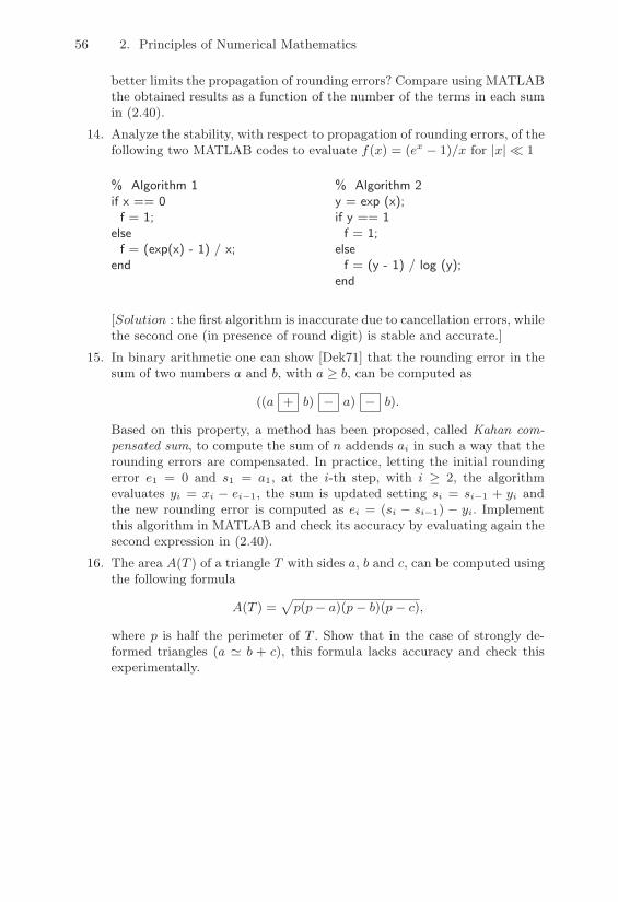
56 2. Principles of Numerical Mathematics
better limits the propagation of rounding errors? Compare using MATLABthe obtained results as a function of the number of the terms in each sumin (2.40).
14. Analyze the stability, with respect to propagation of rounding errors, of thefollowing two MATLAB codes to evaluate f(x) = (ex % 1)/x for |x|2 1
% Algorithm 1if x == 0f = 1;
elsef = (exp(x) - 1) / x;
end
% Algorithm 2y = exp (x);if y == 1f = 1;
elsef = (y - 1) / log (y);
end
[Solution : the first algorithm is inaccurate due to cancellation errors, whilethe second one (in presence of round digit) is stable and accurate.]
15. In binary arithmetic one can show [Dek71] that the rounding error in thesum of two numbers a and b, with a ! b, can be computed as
((a + b) % a) % b).
Based on this property, a method has been proposed, called Kahan com-pensated sum, to compute the sum of n addends ai in such a way that therounding errors are compensated. In practice, letting the initial roundingerror e1 = 0 and s1 = a1, at the i-th step, with i ! 2, the algorithmevaluates yi = xi % ei%1, the sum is updated setting si = si%1 + yi andthe new rounding error is computed as ei = (si % si%1) % yi. Implementthis algorithm in MATLAB and check its accuracy by evaluating again thesecond expression in (2.40).
16. The area A(T ) of a triangle T with sides a, b and c, can be computed usingthe following formula
A(T ) =3
p(p% a)(p% b)(p% c),
where p is half the perimeter of T . Show that in the case of strongly de-formed triangles (a 0 b + c), this formula lacks accuracy and check thisexperimentally.

3Direct Methods for the Solution ofLinear Systems
A system of m linear equations in n unknowns consists of a set of algebraicrelations of the form
n(
j=1
aijxj = bi, i = 1, . . . ,m (3.1)
where xj are the unknowns, aij are the coe"cients of the system and biare the components of the right hand side. System (3.1) can be more con-veniently written in matrix form as
Ax = b, (3.2)
where we have denoted by A = (aij) ! Cm!n the coe"cient matrix, byb=(bi) ! Cm the right side vector and by x=(xi) ! Cn the unknownvector, respectively. We call a solution of (3.2) any n-tuple of values xi
which satisfies (3.1).In this chapter we shall be mainly dealing with real-valued square systems
of order n, that is, systems of the form (3.2) with A ! Rn!n and b ! Rn.In such cases existence and uniqueness of the solution of (3.2) are ensuredif one of the following (equivalent) hypotheses holds:
1. A is invertible;
2. rank(A)=n;
3. the homogeneous system Ax=0 admits only the null solution.

58 3. Direct Methods for the Solution of Linear Systems
The solution of system (3.2) is formally provided by Cramer’s rule
xj =#j
det(A), j = 1, . . . , n, (3.3)
where #j is the determinant of the matrix obtained by substituting thej-th column of A with the right hand side b. This formula is, however,of little practical use. Indeed, if the determinants are evaluated by therecursive relation (1.4), the computational e!ort of Cramer’s rule is of theorder of (n + 1)! flops and therefore turns out to be unacceptable even forsmall dimensions of A (for instance, a computer able to perform 109 flopsper second would take 9.6 · 1047 years to solve a linear system of only 50equations).For this reason, numerical methods that are alternatives to Cramer’s rulehave been developed. They are called direct methods if they yield the so-lution of the system in a finite number of steps, iterative if they require(theoretically) an infinite number of steps. Iterative methods will be ad-dressed in the next chapter. We notice from now on that the choice betweena direct and an iterative method does not depend only on the theoretical ef-ficiency of the scheme, but also on the particular type of matrix, on memorystorage requirements and, finally, on the architecture of the computer.
3.1 Stability Analysis of Linear Systems
Solving a linear system by a numerical method invariably leads to theintroduction of rounding errors. Only using stable numerical methods cankeep away the propagation of such errors from polluting the accuracy of thesolution. In this section two aspects of stability analysis will be addressed.
Firstly, we will analyze the sensitivity of the solution of (3.2) to changesin the data A and b (forward a priori analysis). Secondly, assuming thatan approximate solution :x of (3.2) is available, we shall quantify the per-turbations on the data A and b in order for :x to be the exact solutionof a perturbed system (backward a priori analysis). The size of these per-turbations will in turn allow us to measure the accuracy of the computedsolution :x by the use of a posteriori analysis.
3.1.1 The Condition Number of a MatrixThe condition number of a matrix A ! Cn!n is defined as
K(A) = +A+ +A"1+, (3.4)
where + · + is an induced matrix norm. In general K(A) depends on thechoice of the norm; this will be made clear by introducing a subscript

3.1 Stability Analysis of Linear Systems 59
into the notation, for instance, K$(A) = +A+$ +A"1+$. More generally,Kp(A) will denote the condition number of A in the p-norm. Remarkableinstances are p = 1, p = 2 and p = , (we refer to Exercise 1 for therelations among K1(A), K2(A) and K$(A)).
As already noticed in Example 2.3, an increase in the condition numberproduces a higher sensitivity of the solution of the linear system to changesin the data. Let us start by noticing that K(A) ) 1 since
1 = +AA"1+ & +A+ +A"1+ = K(A).
Moreover, K(A"1) = K(A) and #" ! C with " '= 0, K("A) = K(A).Finally, if A is orthogonal, K2(A) = 1 since +A+2 =
3)(ATA) =
3)(I) = 1
and A"1 = AT . The condition number of a singular matrix is set equal toinfinity.
For p = 2, K2(A) can be characterized as follows. Starting from (1.21),it can be proved that
K2(A) = +A+2 +A"1+2 =(1(A)(n(A)
where (1(A) and (n(A) are the maximum and minimum singular values ofA (see Property 1.7). As a consequence, in the case of symmetric positivedefinite matrices we have
K2(A) =$max
$min= )(A))(A"1) (3.5)
where $max and $min are the maximum and minimum eigenvalues of A.To check (3.5), notice that
+A+2 =2)(ATA) =
3)(A2) =
3$2max = $max.
Moreover, since $(A"1) = 1/$(A), one gets +A"1+2 = 1/$min from which(3.5) follows. For that reason, K2(A) is called spectral condition number.
Remark 3.1 Define the relative distance of A ! Cn!n from the set ofsingular matrices with respect to the p-norm by
distp(A) = minE+%A+p+A+p
: A + %A is singularF.
It can then be shown that ([Kah66], [Gas83])
distp(A) =1
Kp(A). (3.6)
Equation (3.6) suggests that a matrix A with a high condition numbercan behave like a singular matrix of the form A+%A. In other words, null

60 3. Direct Methods for the Solution of Linear Systems
perturbations in the right hand side do not necessarily yield non vanishingchanges in the solution since, if A+%A is singular, the homogeneous system(A + %A)z = 0 does no longer admit only the null solution. From (3.6) italso follows that if A+%A is nonsingular then
+%A+p+A+p < 1. (3.7)
!
Relation (3.6) seems to suggest that a natural candidate for measuringthe ill-conditioning of a matrix is its determinant, since from (3.3) one isprompted to conclude that small determinants mean nearly-singular matri-ces. However this conclusion is wrong, as there exist examples of matriceswith small (respectively, high) determinants and small (respectively, high)condition numbers (see Exercise 2).
3.1.2 Forward a priori AnalysisIn this section we introduce a measure of the sensitivity of the system tochanges in the data. These changes will be interpreted in Section 3.10 asbeing the e!ects of rounding errors induced by the numerical method usedto solve the system. For a more comprehensive analysis of the subject werefer to [Dat95], [GL89], [Ste73] and [Var62].
Due to rounding errors, a numerical method for solving (3.2) does notprovide the exact solution but only an approximate one, which satisfies aperturbed system. In other words, a numerical method yields an (exact)solution x + "x of the perturbed system
(A + %A)(x + %x) = b + "b. (3.8)
The next result provides an estimate of "x in terms of %A and "b.
Theorem 3.1 Let A ! Rn!n be a nonsingular matrix and %A ! Rn!n besuch that (3.7) is satisfied for a matrix norm + · +. Then, if x! Rn is thesolution of Ax=b with b ! Rn (b '= 0) and "x ! Rn satisfies (3.8) for"b ! Rn,
+"x++x+ & K(A)
1"K(A)+%A+/+A+
4+"b++b+ +
+%A++A+
5. (3.9)
Proof. From (3.7) it follows that the matrix A%1!A has norm less than 1. Then,due to Theorem 1.5, I + A%1!A is invertible and from (1.26) it follows that
&(I + A%1!A)%1& " 11% &A%1!A& "
11% &A%1& &!A& . (3.10)
On the other hand, solving for "x in (3.8) and recalling that Ax = b, one gets
"x = (I + A%1!A)%1A%1("b% !Ax),

3.1 Stability Analysis of Linear Systems 61
from which, passing to the norms and using (3.10), it follows that
&"x& " &A%1&1% &A%1& &!A& (&"b&+ &!A& &x&) .
Finally, dividing both sides by &x& (which is nonzero since b $= 0 and A isnonsingular) and noticing that &x& ! &b&/&A&, the result follows. !
Well-conditioning alone is not enough to yield an accurate solution of thelinear system. It is indeed crucial, as pointed out in Chapter 2, to resort tostable algorithms. Conversely, ill-conditioning does not necessarily excludethat for particular choices of the right side b the overall conditioning of thesystem is good (see Exercise 4).A particular case of Theorem 3.1 is the following.
Theorem 3.2 Assume that the conditions of Theorem 3.1 hold and let%A = 0. Then
1K(A)
+"b++b+ & +"x+
+x+ & K(A)+"b++b+ . (3.11)
Proof. We will prove only the first inequality since the second one directlyfollows from (3.9). Relation "x = A%1"b yields &"b& " &A& &"x&. Multiplyingboth sides by &x& and recalling that &x& " &A%1& &b& it follows that &x& &"b& "K(A)&b& &"x&, which is the desired inequality. !
In order to employ the inequalities (3.10) and (3.11) in the analysis ofpropagation of rounding errors in the case of direct methods, +%A+ and+"b+ should be bounded in terms of the dimension of the system and ofthe characteristics of the floating-point arithmetic that is being used.
It is indeed reasonable to expect that the perturbations induced by amethod for solving a linear system are such that +%A+ & '+A+ and +"b+ &'+b+, ' being a positive number that depends on the roundo! unit u (forexample, we shall assume henceforth that ' = #1"t, where # is the baseand t is the number of digits of the mantissa of the floating-point systemF). In such a case (3.9) can be completed by the following theorem.
Theorem 3.3 Assume that +%A+ & '+A+, +"b+ & '+b+ with ' ! R+ and%A ! Rn!n, "b ! Rn. Then, if 'K(A) < 1 the following inequalities hold
+x + "x++x+ & 1 + 'K(A)
1" 'K(A), (3.12)
+"x++x+ & 2'
1" 'K(A)K(A). (3.13)

62 3. Direct Methods for the Solution of Linear Systems
Proof. From (3.8) it follows that (I + A%1!A)(x+ "x) = x+ A%1"b. Moreover,since ,K(A) < 1 and &!A& " ,&A& it turns out that I + A%1!A is nonsingular.Taking the inverse of such a matrix and passing to the norms we get &x+ "x& "&(I + A%1!A)%1&
8&x&+ ,&A%1& &b&
9. From Theorem 1.5 it then follows that
&x + "x& " 11% &A%1!A&
8&x&+ ,&A%1& &b&
9,
which implies (3.12), since &A%1!A& " ,K(A) and &b& " &A& &x&.Let us prove (3.13). Subtracting (3.2) from (3.8) it follows that
A"x = %!A(x + "x) + "b.
Inverting A and passing to the norms, the following inequality is obtained
&"x& " &A%1!A& &x + "x&+ &A%1& &"b&
" ,K(A)&x + "x&+ ,&A%1& &b&.(3.14)
Dividing both sides by &x& and using the triangular inequality &x+"x& " &"x&+&x&, we finally get (3.13). !
Remarkable instances of perturbations %A and "b are those for which|%A| & '|A| and |"b| & '|b| with ' ) 0. Hereafter, the absolute valuenotation B = |A| denotes the matrix n % n having entries bij = |aij | withi, j = 1, . . . , n and the inequality C & D, with C,D ! Rm!n has thefollowing meaning
cij & dij for i = 1, . . . ,m, j = 1, . . . , n.
If + · +$ is considered, from (3.14) it follows that
+"x+$+x+$
& '+ |A"1| |A| |x| + |A"1| |b| +$(1" '+ |A"1| |A| +$)+x+$
& 2'1" '+ |A"1| |A| +$
+ |A"1| |A| +$.
(3.15)
Estimate (3.15) is generally too pessimistic; however, the following compo-nentwise error estimates of "x can be derived from (3.15)
|%xi| & '|rT(i)| |A| |x + "x|, i = 1, . . . , n if "b = 0,
|%xi||xi|
& '|rT(i)| |b||rT(i)b|
, i = 1, . . . , n if %A = 0,(3.16)
being rT(i) the row vector eTi A"1. Estimates (3.16) are more stringent than(3.15), as can be seen in Example 3.1. The first inequality in (3.16) can beused when the perturbed solution x+"x is known, being henceforth x+"xthe solution computed by a numerical method.
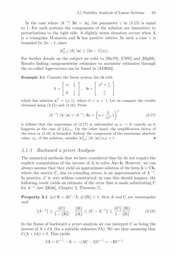
3.1 Stability Analysis of Linear Systems 63
In the case where |A"1| |b| = |x|, the parameter ' in (3.15) is equalto 1. For such systems the components of the solution are insensitive toperturbations to the right side. A slightly worse situation occurs when Ais a triangular M-matrix and b has positive entries. In such a case ' isbounded by 2n" 1, since
|rT(i)| |A| |x| & (2n" 1)|xi|.
For further details on the subject we refer to [Ske79], [CI95] and [Hig89].Results linking componentwise estimates to normwise estimates throughthe so-called hypernorms can be found in [ADR92].
Example 3.1 Consider the linear system Ax=b with
A =
"
$$ 1
!
0 1!
%
' , b =
"
$$2 + 1
!
1!
%
'
which has solution xT = ($, 1), where 0 < $ < 1. Let us compare the resultsobtained using (3.15) and (3.16). From
|A%1| |A| |x| = |A%1| |b| =4$ +
2$2 , 1
5T
(3.17)
it follows that the supremum of (3.17) is unbounded as $ , 0, exactly as ithappens in the case of &A&!. On the other hand, the amplification factor ofthe error in (3.16) is bounded. Indeed, the component of the maximum absolutevalue, x2, of the solution, satisfies |rT(2)| |A| |x|/|x2| = 1. •
3.1.3 Backward a priori AnalysisThe numerical methods that we have considered thus far do not require theexplicit computation of the inverse of A to solve Ax=b. However, we canalways assume that they yield an approximate solution of the form :x = Cb,where the matrix C, due to rounding errors, is an approximation of A"1.In practice, C is very seldom constructed; in case this should happen, thefollowing result yields an estimate of the error that is made substituting Cfor A"1 (see [IK66], Chapter 2, Theorem 7).
Property 3.1 Let R = AC" I; if +R+ < 1, then A and C are nonsingularand
+A"1+ & +C+1" +R+ ,
+R++A+ & +C"A"1+ & +C+ +R+
1" +R+ . (3.18)
In the frame of backward a priori analysis we can interpret C as being theinverse of A + %A (for a suitable unknown %A). We are thus assuming thatC(A + %A) = I. This yields
%A = C"1 "A = "(AC" I)C"1 = "RC"1

64 3. Direct Methods for the Solution of Linear Systems
and, as a consequence, if +R+ < 1 it turns out that
+%A+ & +R+ +A+1" +R+ , (3.19)
having used the first inequality in (3.18), where A is assumed to be anapproximation of the inverse of C (notice that the roles of C and A can beinterchanged).
3.1.4 A posteriori AnalysisHaving approximated the inverse of A by a matrix C turns into having anapproximation of the solution of the linear system (3.2). Let us denote byy a known approximate solution. The aim of the a posteriori analysis is torelate the (unknown) error e = y " x to quantities that can be computedusing y and C.
The starting point of the analysis relies on the fact that the residualvector r = b " Ay is in general nonzero, since y is just an approximationto the unknown exact solution. The residual can be related to the errorthrough Property 3.1 as follows. We have e = A"1(Ay" b) = "A"1r andthus, if +R+ < 1 then
+e+ & +r+ +C+1" +R+ . (3.20)
Notice that the estimate does not necessarily require y to coincide withthe solution :x = Cb of the backward a priori analysis. One could thereforethink of computing C only for the purpose of using the estimate (3.20) (forinstance, in the case where (3.2) is solved through the Gauss eliminationmethod, one can compute C a posteriori using the LU factorization of A,see Sections 3.3 and 3.3.1).
We conclude by noticing that if "b is interpreted in (3.11) as being theresidual of the computed solution y = x + %x, it also follows that
+e++x+ & K(A)
+r++b+ . (3.21)
The estimate (3.21) is not used in practice since the computed residualis a!ected by rounding errors. A more significant estimate (in the + · +$norm) is obtained letting :r = fl(b " Ay) and assuming that :r = r + "rwith |"r| & 'n+1(|A| |y|+ |b|), where 'n+1 = (n+ 1)u/(1" (n+ 1)u) > 0,from which we have
+e+$+y+$
& + |A"1|(|:r| + 'n+1(|A||y| + |b|))+$+y+$
.
Formulae like this last one are implemented in the library for linear algebraLAPACK (see [ABB+92]).

3.2 Solution of Triangular Systems 65
3.2 Solution of Triangular Systems
Consider the nonsingular 3%3 lower triangular system"
$l11 0 0l21 l22 0l31 l32 l33
%
'
"
$x1x2x3
%
' =
"
$b1b2b3
%
' .
Since the matrix is nonsingular, its diagonal entries lii, i = 1, 2, 3, arenon vanishing, hence we can solve sequentially for the unknown valuesxi, i = 1, 2, 3 as follows
x1 = b1/l11,x2 = (b2 " l21x1)/l22,x3 = (b3 " l31x1 " l32x2)/l33.
This algorithm can be extended to systems n % n and is called forwardsubstitution. In the case of a system Lx=b, with L being a nonsingularlower triangular matrix of order n (n ) 2), the method takes the form
x1 =b1l11
,
xi =1lii
G
Hbi "i"1(
j=1
lijxj
I
J , i = 2, . . . , n.(3.22)
The number of multiplications and divisions to execute the algorithm isequal to n(n+1)/2, while the number of sums and subtractions is n(n"1)/2.The global operation count for (3.22) is thus n2 flops.
Similar conclusions can be drawn for a linear system Ux=b, where Uis a nonsingular upper triangular matrix of order n (n ) 2). In this casethe algorithm is called backward substitution and in the general case canbe written as
xn =bnunn
,
xi =1uii
G
Hbi "n(
j=i+1
uijxj
I
J , i = n" 1, . . . , 1.(3.23)
Its computational cost is still n2 flops.
3.2.1 Implementation of Substitution MethodsEach i-th step of algorithm (3.22) requires performing the scalar productbetween the row vector L(i, 1 : i " 1) (this notation denoting the vectorextracted from matrix L taking the elements of the i-th row from the first

66 3. Direct Methods for the Solution of Linear Systems
to the (i-1)-th column) and the column vector x(1 : i " 1). The access tomatrix L is thus by row; for that reason, the forward substitution algorithm,when implemented in the form above, is called row-oriented.
Its coding is reported in Program 1 (the Program mat square that iscalled by forward row merely checks that L is a square matrix).
Program 1 - forward row : Forward substitution: row-oriented version
function [x]=forward row(L,b)[n]=mat square(L); x(1) = b(1)/L(1,1);for i = 2:n, x (i) = (b(i)-L(i,1:i-1)*(x(1:i-1))’)/L(i,i); endx=x’;
To obtain a column-oriented version of the same algorithm, we take ad-vantage of the fact that i-th component of the vector x, once computed,can be conveniently eliminated from the system.
An implementation of such a procedure, where the solution x is over-written on the right vector b, is reported in Program 2.Program 2 - forward col : Forward substitution: column-oriented version
function [b]=forward col(L,b)[n]=mat square(L);for j=1:n-1,
b(j)= b(j)/L(j,j); b(j+1:n)=b(j+1:n)-b(j)*L(j+1:n,j);end; b(n) = b(n)/L(n,n);
Implementing the same algorithm by a row-oriented rather than a column-oriented approach, might dramatically change its performance (but of course,not the solution). The choice of the form of implementation must thereforebe subordinated to the specific hardware that is used.
Similar considerations hold for the backward substitution method, pre-sented in (3.23) in its row-oriented version.In Program 3 only the column-oriented version of the algorithm is coded.As usual, the vector x is overwritten on b.Program 3 - backward col : Backward substitution: column-oriented ver-sion
function [b]=backward col(U,b)[n]=mat square(U);for j = n:-1:2,
b(j)=b(j)/U(j,j); b(1:j-1)=b(1:j-1)-b(j)*U(1:j-1,j);end; b(1) = b(1)/U(1,1);
When large triangular systems must be solved, only the triangular portionof the matrix should be stored leading to considerable saving of memoryresources.
3.2 Solution of Triangular Systems 67
3.2.2 Rounding Error AnalysisThe analysis developed so far has not accounted for the presence of round-ing errors. When including these, the forward and backward substitutionalgorithms no longer yield the exact solutions to the systems Lx=b andUy=b, but rather provide approximate solutions :x that can be regardedas being exact solutions to the perturbed systems
(L + %L):x = b, (U + %U):x = b,
where %L = (%lij) and %U = (%uij) are perturbation matrices. In orderto apply the estimates (3.9) carried out in Section 3.1.2, we must provideestimates of the perturbation matrices, %L and %U, as a function of theentries of L and U, of their size and of the characteristics of the floating-point arithmetic. For this purpose, it can be shown that
|%T| & nu1" nu
|T|, (3.24)
where T is equal to L or U, u = 12#
1"t is the roundo! unit defined in (2.34).Clearly, if nu < 1 from (3.24) it turns out that, using a Taylor expansion,|%T| & nu|T| + O(u2). Moreover, from (3.24) and (3.9) it follows that, ifnuK(T) < 1, then
+x" :x++x+ & nuK(T)
1" nuK(T)= nuK(T) + O(u2) (3.25)
for the norms + · +1, + · +$ and the Frobenius norm. If u is su"cientlysmall (as typically happens), the perturbations introduced by the roundingerrors in the solution of a triangular system can thus be neglected. Asa consequence, the accuracy of the solution computed by the forward orbackward substitution algorithm is generally very high.
These results can be improved by introducing some additional assump-tions on the entries of L or U. In particular, if the entries of U are suchthat |uii| ) |uij | for any j > i, then
|xi " :xi| & 2n"i+1 nu1" nu
maxj+i
|:xj |, 1 & i & n.
The same result holds if T=L, provided that |lii| ) |lij | for any j < i, or ifL and U are diagonally dominant. The previous estimates will be employedin Sections 3.3.1 and 3.4.2.
For the proofs of the results reported so far, see [FM67], [Hig89] and[Hig88].
3.2.3 Inverse of a Triangular MatrixThe algorithm (3.23) can be employed to explicitly compute the inverseof an upper triangular matrix. Indeed, given an upper triangular matrix

68 3. Direct Methods for the Solution of Linear Systems
U, the column vectors vi of the inverse V=(v1, . . . ,vn) of U satisfy thefollowing linear systems
Uvi = ei, i = 1, . . . , n (3.26)
where {ei} is the canonical basis of Rn (defined in Example 1.3). Solvingfor vi thus requires the application of algorithm (3.23) n times to (3.26).
This procedure is quite ine"cient since at least half the entries of theinverse of U are null. Let us take advantage of this as follows. Denote byv*k = (v*1k, . . . , v
*kk)
T the vector of size k such that
U(k)v*k = lk k = 1, . . . , n (3.27)
where U(k) is the principal submatrix of U of order k and lk the vector ofRk having null entries, except the first one which is equal to 1. Systems(3.27) are upper triangular, but have order k and can be again solved usingthe method (3.23). We end up with the following inversion algorithm forupper triangular matrices: for k = n, n" 1, . . . , 1 compute
v*kk = u"1kk ,
v*ik = "u"1ii
k(
j=i+1
uijv*jk, for i = k " 1, k " 2, . . . , 1. (3.28)
At the end of this procedure the vectors v*k furnish the non vanishing entries
of the columns of U"1. The algorithm requires about n3/3 + (3/4)n2 flops.Once again, due to rounding errors, the algorithm (3.28) no longer yieldsthe exact solution, but an approximation of it. The error that is introducedcan be estimated using the backward a priori analysis carried out in Section3.1.3.
A similar procedure can be constructed from (3.22) to compute the in-verse of a lower triangular system.
3.3 The Gaussian Elimination Method (GEM) andLU Factorization
The Gaussian elimination method aims at reducing the system Ax=b to anequivalent system (that is, having the same solution) of the form Ux=:b,where U is an upper triangular matrix and :b is an updated right sidevector. This latter system can then be solved by the backward substitutionmethod. Let us denote the original system by A(1)x = b(1). During thereduction procedure we basically employ the property which states thatreplacing one of the equations by the di!erence between this equation andanother one multiplied by a non null constant yields an equivalent system(i.e., one with the same solution).

3.3 The Gaussian Elimination Method (GEM) and LU Factorization 69
Thus, consider a nonsingular matrix A ! Rn!n, and suppose that thediagonal entry a11 is non vanishing. Introducing the multipliers
mi1 =a(1)i1
a(1)11
, i = 2, 3, . . . , n,
where a(1)ij denote the elements of A(1), it is possible to eliminate the un-
known x1 from the rows other than the first one by simply subtractingfrom row i, with i = 2, . . . , n, the first row multiplied by mi1 and doingthe same on the right side. If we now define
a(2)ij = a(1)
ij "mi1a(1)1j , i, j = 2, . . . , n,
b(2)i = b(1)i "mi1b(1)1 , i = 2, . . . , n,
where b(1)i denote the components of b(1), we get a new system of the form
"
####$
a(1)11 a(1)
12 . . . a(1)1n
0 a(2)22 . . . a(2)
2n...
......
0 a(2)n2 . . . a(2)
nn
%
&&&&'
"
###$
x1x2...xn
%
&&&'=
"
####$
b(1)1
b(2)2...
b(2)n
%
&&&&',
which we denote by A(2)x = b(2), that is equivalent to the starting one.Similarly, we can transform the system in such a way that the unknownx2 is eliminated from rows 3, . . . , n. In general, we end up with the finitesequence of systems
A(k)x = b(k), 1 & k & n, (3.29)
where, for k ) 2, matrix A(k) takes the following form
A(k) =
"
#########$
a(1)11 a(1)
12 . . . . . . . . . a(1)1n
0 a(2)22 a(2)
2n...
. . ....
0 . . . 0 a(k)kk . . . a(k)
kn...
......
...0 . . . 0 a(k)
nk . . . a(k)nn
%
&&&&&&&&&'
,

70 3. Direct Methods for the Solution of Linear Systems
having assumed that a(i)ii '= 0 for i = 1, . . . , k" 1. It is clear that for k = n
we obtain the upper triangular system A(n)x = b(n)
"
#######$
a(1)11 a(1)
12 . . . . . . a(1)1n
0 a(2)22 a(2)
2n...
. . ....
0. . .
...0 a(n)
nn
%
&&&&&&&'
"
######$
x1x2......xn
%
&&&&&&'=
"
#######$
b(1)1
b(2)2......
b(n)n
%
&&&&&&&'
.
Consistently with the notations that have been previously introduced, wedenote by U the upper triangular matrix A(n). The entries a(k)
kk are calledpivots and must obviously be non null for k = 1, . . . , n" 1.
In order to highlight the formulae which transform the k-th system intothe k + 1-th one, for k = 1, . . . , n" 1 we assume that a(k)
kk '= 0 and definethe multiplier
mik =a(k)ik
a(k)kk
, i = k + 1, . . . , n. (3.30)
Then we let
a(k+1)ij = a(k)
ij "mika(k)kj , i, j = k + 1, . . . , n
b(k+1)i = b(k)
i "mikb(k)k , i = k + 1, . . . , n.
(3.31)
Example 3.2 Let us use GEM to solve the following system
(A(1)x = b(1))
)***+
***,
x1 + 12x2 + 1
3x3 = 116
12x1 + 1
3x2 + 14x3 = 13
12
13x1 + 1
4x2 + 15x3 = 47
60
,
which admits the solution x=(1, 1, 1)T . At the first step we compute the mul-tipliers m21 = 1/2 and m31 = 1/3, and subtract from the second and thirdequation of the system the first row multiplied by m21 and m31, respectively. Weobtain the equivalent system
(A(2)x = b(2))
)***+
***,
x1 + 12x2 + 1
3x3 = 116
0 + 112x2 + 1
12x3 = 16
0 + 112x2 + 4
45x3 = 31180
.
If we now subtract the second row multiplied by m32 = 1 from the third one, weend up with the upper triangular system
(A(3)x = b(3))
)***+
***,
x1 + 12x2 + 1
3x3 = 116
0 + 112x2 + 1
12x3 = 16
0 + 0 + 1180x3 = 1
180
,
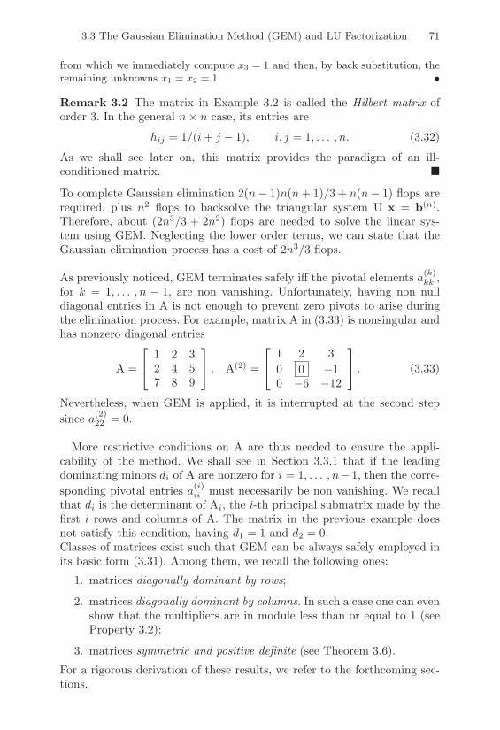
3.3 The Gaussian Elimination Method (GEM) and LU Factorization 71
from which we immediately compute x3 = 1 and then, by back substitution, theremaining unknowns x1 = x2 = 1. •
Remark 3.2 The matrix in Example 3.2 is called the Hilbert matrix oforder 3. In the general n% n case, its entries are
hij = 1/(i + j " 1), i, j = 1, . . . , n. (3.32)
As we shall see later on, this matrix provides the paradigm of an ill-conditioned matrix. !To complete Gaussian elimination 2(n" 1)n(n + 1)/3 + n(n" 1) flops arerequired, plus n2 flops to backsolve the triangular system U x = b(n).Therefore, about (2n3/3 + 2n2) flops are needed to solve the linear sys-tem using GEM. Neglecting the lower order terms, we can state that theGaussian elimination process has a cost of 2n3/3 flops.
As previously noticed, GEM terminates safely i! the pivotal elements a(k)kk ,
for k = 1, . . . , n " 1, are non vanishing. Unfortunately, having non nulldiagonal entries in A is not enough to prevent zero pivots to arise duringthe elimination process. For example, matrix A in (3.33) is nonsingular andhas nonzero diagonal entries
A =
"
$1 2 32 4 57 8 9
%
' , A(2) =
"
$1 2 30 0 "10 "6 "12
%
' . (3.33)
Nevertheless, when GEM is applied, it is interrupted at the second stepsince a(2)
22 = 0.
More restrictive conditions on A are thus needed to ensure the appli-cability of the method. We shall see in Section 3.3.1 that if the leadingdominating minors di of A are nonzero for i = 1, . . . , n" 1, then the corre-sponding pivotal entries a(i)
ii must necessarily be non vanishing. We recallthat di is the determinant of Ai, the i-th principal submatrix made by thefirst i rows and columns of A. The matrix in the previous example doesnot satisfy this condition, having d1 = 1 and d2 = 0.Classes of matrices exist such that GEM can be always safely employed inits basic form (3.31). Among them, we recall the following ones:
1. matrices diagonally dominant by rows;
2. matrices diagonally dominant by columns. In such a case one can evenshow that the multipliers are in module less than or equal to 1 (seeProperty 3.2);
3. matrices symmetric and positive definite (see Theorem 3.6).
For a rigorous derivation of these results, we refer to the forthcoming sec-tions.

72 3. Direct Methods for the Solution of Linear Systems
3.3.1 GEM as a Factorization MethodIn this section we show how GEM is equivalent to performing a factorizationof the matrix A into the product of two matrices, A=LU, with U=A(n).Since L and U depend only on A and not on the right hand side, the samefactorization can be reused when solving several linear systems having thesame matrix A but di!erent right hand side b, with a considerable reductionof the operation count (indeed, the main computational e!ort, about 2n3/3flops, is spent in the elimination procedure).
Let us go back to Example 3.2 concerning the Hilbert matrix H3. Inpractice, to pass from A(1)=H3 to the matrix A(2) at the second step, wehave multiplied the system by the matrix
M1 =
"
###$
1 0 0
" 12 1 0
" 13 0 1
%
&&&'=
"
###$
1 0 0
"m21 1 0
"m31 0 1
%
&&&'.
Indeed,
M1A = M1A(1) =
"
###$
1 12
13
0 112
112
0 112
445
%
&&&'= A(2).
Similarly, to perform the second (and last) step of GEM, we must multiplyA(2) by the matrix
M2 =
"
###$
1 0 0
0 1 0
0 "1 1
%
&&&'=
"
###$
1 0 0
0 1 0
0 "m32 1
%
&&&',
where A(3) = M2A(2). Therefore
M2M1A = A(3) = U. (3.34)
On the other hand, matrices M1 and M2 are lower triangular, their productis still lower triangular, as is their inverse; thus, from (3.34) one gets
A = (M2M1)"1U = LU,
which is the desired factorization of A.This identity can be generalized as follows. Setting
mk = (0, . . . , 0,mk+1,k, . . . ,mn,k)T ! Rn

3.3 The Gaussian Elimination Method (GEM) and LU Factorization 73
and defining
Mk =
"
########$
1 . . . 0 0 . . . 0...
. . ....
......
0 1 0 00 "mk+1,k 1 0...
......
.... . .
...0 . . . "mn,k 0 . . . 1
%
&&&&&&&&'
= In "mkeTk
as the k-th Gaussian transformation matrix, one finds out that
(Mk)ip = %ip " (mkeTk )ip = %ip "mik%kp, i, p = 1, . . . , n.
On the other hand, from (3.31) we have that
a(k+1)ij = a(k)
ij "mik%kka(k)kj =
n(
p=1
(%ip "mik%kp)a(k)pj , i, j = k + 1, . . . , n,
or, equivalently,
A(k+1) = MkA(k). (3.35)
As a consequence, at the end of the elimination process the matrices Mk,with k = 1, . . . , n" 1, and the matrix U have been generated such that
Mn"1Mn"2 . . .M1A = U.
The matrices Mk are unit lower triangular with inverse given by
M"1k = 2In "Mk = In + mkeTk , (3.36)
where (mieTi )(mjeTj ) are equal to the null matrix if i '= j. As a consequence
A = M"11 M"1
2 . . .M"1n"1U
= (In + m1eT1 )(In + m2eT2 ) . . . (In + mn"1eTn"1)U
=
6
In +n"1(
i=1
mieTi
7
U
=
"
#############$
1 0 . . . . . . 0
m21 1...
... m32. . .
...
......
. . . 0
mn1 mn2 . . . mn,n"1 1
%
&&&&&&&&&&&&&'
U.
(3.37)

74 3. Direct Methods for the Solution of Linear Systems
Defining L = (Mn"1Mn"2 . . .M1)"1 = M"11 . . .M"1
n"1, it follows that
A = LU.
We notice that, due to (3.37), the subdiagonal entries of L are the multi-pliers mik produced by GEM, while the diagonal entries are equal to one.
Once the matrices L and U have been computed, solving the linear systemconsists only of solving successively the two triangular systems
Ly = b
Ux = y.
The computational cost of the factorization process is obviously the sameas that required by GEM.
The following result establishes a link between the leading dominantminors of a matrix and its LU factorization induced by GEM.
Theorem 3.4 Let A ! Rn!n. The LU factorization of A with lii = 1 fori = 1, . . . , n exists and is unique i! the principal submatrices Ai of A oforder i = 1, . . . , n" 1 are nonsingular.
Proof. The existence of the LU factorization can be proved following the stepsof the GEM. Here we prefer to pursue an alternative approach, which allows forproving at the same time both existence and uniqueness and that will be usedagain in later sections.
Let us assume that the leading minors Ai of A are nonsingular for i = 1, . . . , n%1 and prove, by induction on i, that under this hypothesis the LU factorizationof A(= An) with lii = 1 for i = 1, . . . , n, exists and is unique.
The property is obviously true if i = 1. Assume therefore that there exists anunique LU factorization of Ai%1 of the form Ai%1 = L(i%1)U(i%1) with l(i%1)
kk = 1for k = 1, . . . , i % 1, and show that there exists an unique factorization also forAi. We partition Ai by block matrices as
Ai =
"
$Ai%1 c
dT aii
%
'
and look for a factorization of Ai of the form
Ai = L(i)U(i) =
"
$L(i%1) 0
lT 1
%
'
"
$U(i%1) u
0T uii
%
' , (3.38)
having also partitioned by blocks the factors L(i) and U(i). Computing the prod-uct of these two factors and equating by blocks the elements of Ai, it turns outthat the vectors l and u are the solutions to the linear systems L(i%1)u = c,lTU(i%1) = dT .
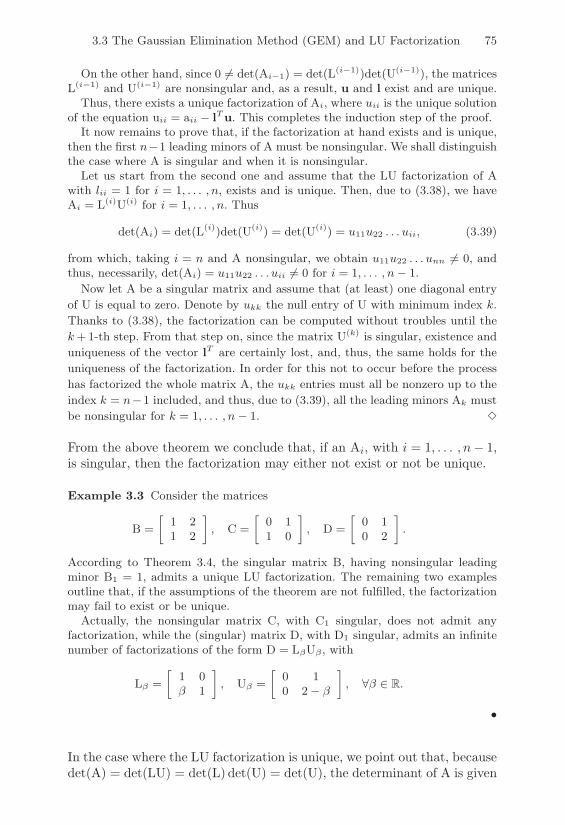
3.3 The Gaussian Elimination Method (GEM) and LU Factorization 75
On the other hand, since 0 $= det(Ai%1) = det(L(i%1))det(U(i%1)), the matricesL(i%1) and U(i%1) are nonsingular and, as a result, u and l exist and are unique.
Thus, there exists a unique factorization of Ai, where uii is the unique solutionof the equation uii = aii % lTu. This completes the induction step of the proof.
It now remains to prove that, if the factorization at hand exists and is unique,then the first n%1 leading minors of A must be nonsingular. We shall distinguishthe case where A is singular and when it is nonsingular.
Let us start from the second one and assume that the LU factorization of Awith lii = 1 for i = 1, . . . , n, exists and is unique. Then, due to (3.38), we haveAi = L(i)U(i) for i = 1, . . . , n. Thus
det(Ai) = det(L(i))det(U(i)) = det(U(i)) = u11u22 . . . uii, (3.39)
from which, taking i = n and A nonsingular, we obtain u11u22 . . . unn $= 0, andthus, necessarily, det(Ai) = u11u22 . . . uii $= 0 for i = 1, . . . , n% 1.
Now let A be a singular matrix and assume that (at least) one diagonal entryof U is equal to zero. Denote by ukk the null entry of U with minimum index k.Thanks to (3.38), the factorization can be computed without troubles until thek+ 1-th step. From that step on, since the matrix U(k) is singular, existence anduniqueness of the vector lT are certainly lost, and, thus, the same holds for theuniqueness of the factorization. In order for this not to occur before the processhas factorized the whole matrix A, the ukk entries must all be nonzero up to theindex k = n%1 included, and thus, due to (3.39), all the leading minors Ak mustbe nonsingular for k = 1, . . . , n% 1. !
From the above theorem we conclude that, if an Ai, with i = 1, . . . , n" 1,is singular, then the factorization may either not exist or not be unique.
Example 3.3 Consider the matrices
B =-
1 21 2
., C =
-0 11 0
., D =
-0 10 2
..
According to Theorem 3.4, the singular matrix B, having nonsingular leadingminor B1 = 1, admits a unique LU factorization. The remaining two examplesoutline that, if the assumptions of the theorem are not fulfilled, the factorizationmay fail to exist or be unique.
Actually, the nonsingular matrix C, with C1 singular, does not admit anyfactorization, while the (singular) matrix D, with D1 singular, admits an infinitenumber of factorizations of the form D = L"U" , with
L" =-
1 0) 1
., U" =
-0 10 2% )
., )) / R.
•
In the case where the LU factorization is unique, we point out that, becausedet(A) = det(LU) = det(L) det(U) = det(U), the determinant of A is given

76 3. Direct Methods for the Solution of Linear Systems
by
det(A) = u11 · · ·unn.
Let us now recall the following property (referring for its proof to [GL89]or [Hig96]).
Property 3.2 If A is a matrix diagonally dominant by rows or by columns,then the LU factorization of A exists. In particular, if A is diagonally dom-inant by columns, then |lij | & 1 #i, j.
In the proof of Theorem 3.4 we exploited the fact the the diagonal entriesof L are equal to 1. In a similar manner, we could have fixed to 1 thediagonal entries of the upper triangular matrix U, obtaining a variant ofGEM that will be considered in Section 3.3.4.
The freedom in setting up either the diagonal entries of L or those of U,implies that several LU factorizations exist which can be obtained one fromthe other by multiplication with a suitable diagonal matrix (see Section3.4.1).
3.3.2 The E!ect of Rounding ErrorsIf rounding errors are taken into account, the factorization process inducedby GEM yields two matrices, :L and :U, such that :L:U = A+ %A, %A being aperturbation matrix. The size of such a perturbation can be estimated by
|%A| & nu1" nu
|:L| |:U|, (3.40)
where u is the roundo! unit (for the proof of this result we refer to [Hig89]).From (3.40) it is seen that the presence of small pivotal entries can makethe right side of the inequality virtually unbounded, with a consequent lossof control on the size of the perturbation matrix %A. The interest is thusin finding out estimates like (3.40) of the form
|%A| & g(u)|A|,
where g(u) is a suitable function of u. For instance, assuming that :L and:U have nonnegative entries, then since |:L| |:U| = |:L:U| one gets
|:L| |:U| = |:L:U| = |A + %A| & |A| + |%A| & |A| + nu1" nu
|:L| |:U|, (3.41)
from which the desired bound is achieved by taking g(u) = nu/(1" 2nu).The technique of pivoting, examined in Section 3.5, keeps the size of the
pivotal entries under control and makes it possible to obtain estimates like(3.41) for any matrix.

3.3 The Gaussian Elimination Method (GEM) and LU Factorization 77
3.3.3 Implementation of LU FactorizationSince L is a lower triangular matrix with diagonal entries equal to 1 and Uis upper triangular, it is possible (and convenient) to store the LU factor-ization directly in the same memory area that is occupied by the matrix A.More precisely, U is stored in the upper triangular part of A (including thediagonal), whilst L occupies the lower triangular portion of A (the diagonalentries of L are not stored since they are implicitly assumed to be 1).
A coding of the algorithm is reported in Program 4. The output matrixA contains the overwritten LU factorization.Program 4 - lu kji : LU factorization of matrix A. kji version
function [A] = lu kji (A)[n,n]=size(A);for k=1:n-1
A(k+1:n,k)=A(k+1:n,k)/A(k,k);for j=k+1:n, for i=k+1:n
A(i,j)=A(i,j)-A(i,k)*A(k,j);end, end
end
This implementation of the factorization algorithm is commonly referredto as the kji version, due to the order in which the cycles are executed.In a more appropriate notation, it is called the SAXPY " kji version,due to the fact that the basic operation of the algorithm, which consists ofmultiplying a scalar A by a vector X, summing another vector Y and thenstoring the result, is usually called SAXPY (i.e. Scalar A X P lus Y ).
The factorization can of course be executed by following a di!erent order.In general, the forms in which the cycle on index i precedes the cycle onj are called row-oriented, whilst the others are called column-oriented. Asusual, this terminology refers to the fact that the matrix is accessed byrows or by columns.
An example of LU factorization, jki version and column-oriented, is givenin Program 5. This version is commonly called GAXPY " jki, since thebasic operation (a product matrix-vector), is called GAXPY which standsfor Generalized sAXPY (see for further details [DGK84]). In the GAXPYoperation the scalar A of the SAXPY operation is replaced by a matrix.Program 5 - lu jki : LU factorization of matrix A. jki version
function [A] = lu jki (A)[n,n]=size(A);for j=1:n
for k=1:j-1, for i=k+1:nA(i,j)=A(i,j)-A(i,k)*A(k,j);
end, endfor i=j+1:n, A(i,j)=A(i,j)/A(j,j); end
end
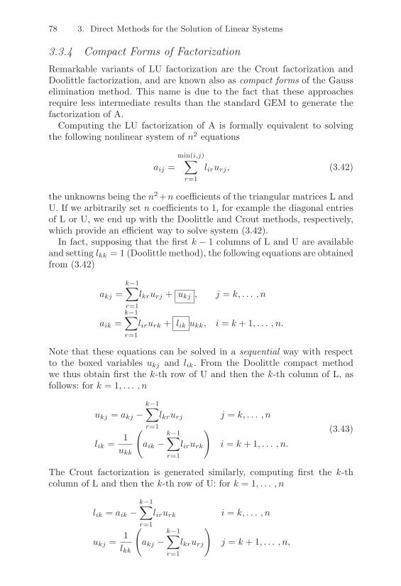
78 3. Direct Methods for the Solution of Linear Systems
3.3.4 Compact Forms of FactorizationRemarkable variants of LU factorization are the Crout factorization andDoolittle factorization, and are known also as compact forms of the Gausselimination method. This name is due to the fact that these approachesrequire less intermediate results than the standard GEM to generate thefactorization of A.
Computing the LU factorization of A is formally equivalent to solvingthe following nonlinear system of n2 equations
aij =min(i,j)(
r=1
lirurj , (3.42)
the unknowns being the n2 +n coe"cients of the triangular matrices L andU. If we arbitrarily set n coe"cients to 1, for example the diagonal entriesof L or U, we end up with the Doolittle and Crout methods, respectively,which provide an e"cient way to solve system (3.42).
In fact, supposing that the first k " 1 columns of L and U are availableand setting lkk = 1 (Doolittle method), the following equations are obtainedfrom (3.42)
akj =k"1(
r=1
lkrurj + ukj , j = k, . . . , n
aik =k"1(
r=1
lirurk + lik ukk, i = k + 1, . . . , n.
Note that these equations can be solved in a sequential way with respectto the boxed variables ukj and lik. From the Doolittle compact methodwe thus obtain first the k-th row of U and then the k-th column of L, asfollows: for k = 1, . . . , n
ukj = akj "k"1(
r=1
lkrurj j = k, . . . , n
lik =1
ukk
6
aik "k"1(
r=1
lirurk
7
i = k + 1, . . . , n.(3.43)
The Crout factorization is generated similarly, computing first the k-thcolumn of L and then the k-th row of U: for k = 1, . . . , n
lik = aik "k"1(
r=1
lirurk i = k, . . . , n
ukj =1lkk
6
akj "k"1(
r=1
lkrurj
7
j = k + 1, . . . , n,

3.4 Other Types of Factorization 79
where we set ukk = 1. Recalling the notations introduced above, the Doolit-tle factorization is nothing but the ijk version of GEM.
We provide in Program 6 the implementation of the Doolittle scheme.Notice that now the main computation is a dot product, so this scheme isalso known as the DOT " ijk version of GEM.Program 6 - lu ijk : LU factorization of the matrix A: ijk version
function [A] = lu ijk (A)[n,n]=size(A);for i=1:n
for j=2:iA(i,j-1)=A(i,j-1)/A(j-1,j-1);for k=1:j-1, A(i,j)=A(i,j)-A(i,k)*A(k,j); end
endfor j=i+1:n
for k=1:i-1, A(i,j)=A(i,j)-A(i,k)*A(k,j); endend
end
3.4 Other Types of Factorization
We now address factorizations suitable for symmetric and rectangular ma-trices.
3.4.1 LDMT FactorizationIt is possible to devise other types of factorizations of A removing thehypothesis that the elements of L are equal to one. Specifically, we willaddress some variants where the factorization of A is of the form
A = LDMT .
where L, MT and D are lower triangular, upper triangular and diagonalmatrices, respectively.
After the construction of this factorization, the resolution of the systemcan be carried out solving first the lower triangular system Ly=b, then thediagonal one Dz=y, and finally the upper triangular system MTx=z, witha cost of n2 + n flops. In the symmetric case, we obtain M = L and theLDLT factorization can be computed with half the cost (see Section 3.4.2).
The LDLT factorization enjoys a property analogous to the one in The-orem 3.4 for the LU factorization. In particular, the following result holds.
Theorem 3.5 If all the principal minors of a matrix A! Rn!n are nonzerothen there exist a unique diagonal matrix D, a unique unit lower triangu-lar matrix L and a unique unit upper triangular matrix MT , such thatA = LDMT .
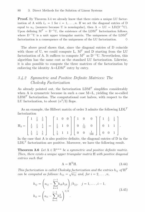
80 3. Direct Methods for the Solution of Linear Systems
Proof. By Theorem 3.4 we already know that there exists a unique LU factor-ization of A with lii = 1 for i = 1, . . . , n. If we set the diagonal entries of Dequal to uii (nonzero because U is nonsingular), then A = LU = LD(D%1U).Upon defining MT = D%1U, the existence of the LDMT factorization follows,where D%1U is a unit upper triangular matrix. The uniqueness of the LDMT
factorization is a consequence of the uniqueness of the LU factorization. !
The above proof shows that, since the diagonal entries of D coincidewith those of U, we could compute L, MT and D starting from the LUfactorization of A. It su"ces to compute MT as D"1U. Nevertheless, thisalgorithm has the same cost as the standard LU factorization. Likewise,it is also possible to compute the three matrices of the factorization byenforcing the identity A=LDMT entry by entry.
3.4.2 Symmetric and Positive Definite Matrices: TheCholesky Factorization
As already pointed out, the factorization LDMT simplifies considerablywhen A is symmetric because in such a case M=L, yielding the so-calledLDMT factorization. The computational cost halves, with respect to theLU factorization, to about (n3/3) flops.
As an example, the Hilbert matrix of order 3 admits the following LDLT
factorization
H3 =
"
###$
1 12
13
12
13
14
13
14
15
%
&&&'=
"
###$
1 0 0
12 1 0
13 1 1
%
&&&'
"
###$
1 0 0
0 112 0
0 0 1180
%
&&&'
"
###$
1 12
13
0 1 1
0 0 1
%
&&&'.
In the case that A is also positive definite, the diagonal entries of D in theLDLT factorization are positive. Moreover, we have the following result.
Theorem 3.6 Let A ! Rn!n be a symmetric and positive definite matrix.Then, there exists a unique upper triangular matrix H with positive diagonalentries such that
A = HTH. (3.44)
This factorization is called Cholesky factorization and the entries hij of HT
can be computed as follows: h11 =/a11 and, for i = 2, . . . , n,
hij =
6
aij "j"1(
k=1
hikhjk
7
/hjj , j = 1, . . . , i" 1,
hii =
6
aii "i"1(
k=1
h2ik
71/2
.
(3.45)

3.4 Other Types of Factorization 81
Proof. Let us prove the theorem proceeding by induction on the size i of thematrix (as done in Theorem 3.4), recalling that if Ai / Ri&i is symmetric positivedefinite, then all its principal submatrices enjoy the same property.
For i = 1 the result is obviously true. Thus, suppose that it holds for i% 1 andprove that it also holds for i. There exists an upper triangular matrix Hi%1 suchthat Ai%1 = HT
i%1Hi%1. Let us partition Ai as
Ai =-
Ai%1 vvT $
.,
with $ / R+, vT / Ri%1 and look for a factorization of Ai of the form
Ai = HTi Hi =
-HT
i%1 0hT )
. -Hi%1 h0T )
..
Enforcing the equality with the entries of Ai yields the equations HTi%1h = v
and hTh + )2 = $. The vector h is thus uniquely determined, since HTi%1 is
nonsingular. As for ), due to the properties of determinants
0 < det(Ai) = det(HTi ) det(Hi) = )2(det(Hi%1))2,
we can conclude that it must be a real number. As a result, ) ='$% hTh is
the desired diagonal entry and this concludes the inductive argument.Let us now prove formulae (3.45). The fact that h11 =
'a11 is an immediate
consequence of the induction argument for i = 1. In the case of a generic i,relations (3.45)1 are the forward substitution formulae for the solution of thelinear system HT
i%1h = v = (a1i, a2i, . . . , ai%1,i)T , while formulae (3.45)2 statethat ) =
'$% hTh, where $ = aii. !
The algorithm which implements (3.45) requires about (n3/3) flops and itturns out to be stable with respect to the propagation of rounding errors.It can indeed be shown that the upper triangular matrix H is such thatHT H = A + %A, where %A is a pertubation matrix such that +%A+2 &8n(n + 1)u+A+2, when the rounding errors are considered and assumingthat 2n(n + 1)u & 1" (n + 1)u (see [Wil68]).
Also, for the Cholesky factorization it is possible to overwrite the matrixHT in the lower triangular portion of A, without any further memory stor-age. By doing so, both A and the factorization are preserved, noting thatA is stored in the upper triangular section since it is symmetric and thatits diagonal entries can be computed as a11 = h2
11, aii = h2ii +
!i"1k=1 h
2ik,
i = 2, . . . , n.An example of implementation of the Cholesky factorization is coded inProgram 7.Program 7 - chol2 : Cholesky factorization
function [A] = chol2 (A)[n,n]=size(A);

82 3. Direct Methods for the Solution of Linear Systems
for k=1:n-1A(k,k)=sqrt(A(k,k)); A(k+1:n,k)=A(k+1:n,k)/A(k,k);for j=k+1:n, A(j:n,j)=A(j:n,j)-A(j:n,k)*A(j,k); end
endA(n,n)=sqrt(A(n,n));
3.4.3 Rectangular Matrices: The QR FactorizationDefinition 3.1 A matrix A ! Rm!n, with m ) n, admits a QR fac-torization if there exist an orthogonal matrix Q ! Rm!m and an uppertrapezoidal matrix R ! Rm!n with null rows from the n + 1-th one on,such that
A = QR. (3.46)
!
This factorization can be constructed either using suitable transformationmatrices (Givens or Householder matrices, see Section 5.6.1) or using theGram-Schmidt orthogonalization algorithm discussed below.
It is also possible to generate a reduced version of the QR factorization(3.46), as stated in the following result.
Property 3.3 Let A ! Rm!n be a matrix of rank n for which a QR fac-torization is known. Then there exists a unique factorization of A of theform
A = DQDR (3.47)
where DQ and DR are submatrices of Q and R given respectively by
DQ = Q(1 : m, 1 : n), DR = R(1 : n, 1 : n). (3.48)
Moreover, DQ has orthonormal vector columns and DR is upper triangularand coincides with the Cholesky factor H of the symmetric positive definitematrix ATA, that is, ATA = DRT DR.
If A has rank n (i.e., full rank), then the column vectors of Q form anorthonormal basis for the vector space range(A) (defined in (1.5)). As aconsequence, constructing the QR factorization can also be interpreted asa procedure for generating an orthonormal basis for a given set of vectors.If A has rank r < n, the QR factorization does not necessarily yield anorthonormal basis for range(A). However, one can obtain a factorization ofthe form
QTAP =-
R11 R120 0
.,

3.4 Other Types of Factorization 83
n
Am =
m" n
Q
R0
n n
n
m" n
FIGURE 3.1. The reduced factorization. The matrices of the QR factorizationare drawn in dashed lines
where Q is orthogonal, P is a permutation matrix and R11 is a nonsingularupper triangular matrix of order r.
In general, when using the QR factorization, we shall always refer to itsreduced form (3.47) as it finds a remarkable application in the solution ofoverdetermined systems (see Section 3.13).
The matrix factors Q and R in (3.47) can be computed using the Gram-Schmidt orthogonalization. Starting from a set of linearly independent vec-tors, x1, . . . ,xn, this algorithm generates a new set of mutually orthogonalvectors, q1, . . . ,qn, given by
q1 = x1,
qk+1 = xk+1 "k(
i=1
(qi,xk+1)(qi,qi)
qi, k = 1, . . . , n" 1.(3.49)
Denoting by a1, . . . ,an the column vectors of A, we set q1 = a1/+a1+2and, for k = 1, . . . , n" 1, compute the column vectors of Q as
qk+1 = qk+1/+qk+1+2,
where
qk+1 = ak+1 "k(
j=1
(qj ,ak+1)qj .
Next, imposing that A=QR and exploiting the fact that Q is orthogonal(that is, Q"1 = QT ), the entries of R can easily be computed. The overallcomputational cost of the algorithm is of the order of mn2 flops.
It is also worth noting that if A has full rank, the matrix ATA is sym-metric and positive definite (see Section 1.9) and thus it admits a uniqueCholesky factorization of the form HTH. On the other hand, since the or-thogonality of Q implies
HTH = ATA = RT QT QR = RT R,

84 3. Direct Methods for the Solution of Linear Systems
we conclude that R is actually the Cholesky factor H of ATA. Thus, thediagonal entries of R are all nonzero only if A has full rank.The Gram-Schmidt method is of little practical use since the generatedvectors lose their linear independence due to rounding errors. Indeed, infloating-point arithmetic the algorithm produces very small values of +qk+1+2and rkk with a consequent numerical instability and loss of orthogonalityfor matrix Q (see Example 3.4).
These drawbacks suggest employing a more stable version, known asmodified Gram-Schmidt method. At the beginning of the k + 1-th step, theprojections of the vector ak+1 along the vectors q1, . . . , qk are progressivelysubtracted from ak+1. On the resulting vector, the orthogonalization stepis then carried out. In practice, after computing (q1,ak+1)q1 at the k+1-thstep, this vector is immediately subtracted from ak+1. As an example, onelets
a(1)k+1 = ak+1 " (q1,ak+1)q1.
This new vector a(1)k+1 is projected along the direction of q2 and the obtained
projection is subtracted from a(1)k+1, yielding
a(2)k+1 = a(1)
k+1 " (q2,a(1)k+1)q2
and so on, until a(k)k+1 is computed.
It can be checked that a(k)k+1 coincides with the corresponding vector qk+1
in the standard Gram-Schmidt process, since, due to the orthogonality ofvectors q1, q2, . . . , qk,
a(k)k+1 = ak+1 " (q1,ak+1)q1 " (q2,ak+1 " (q1,ak+1)q1) q2 + . . .
= ak+1 "k(
j=1
(qj ,ak+1)qj .
Program 8 implements the modified Gram-Schmidt method. Notice thatit is not possible to overwrite the computed QR factorization on the ma-trix A. In general, the matrix DR is overwritten on A, whilst DQ is storedseparately. The computational cost of the modified Gram-Schmidt methodhas the order of 2mn2 flops.
Program 8 - mod grams : Modified Gram-Schmidt method
function [Q,R] = mod grams(A)[m,n]=size(A);Q=zeros(m,n); Q(1:m,1) = A(1:m,1); R=zeros(n); R(1,1)=1;for k = 1:nR(k,k) = norm (A(1:m,k)); Q(1:m,k) = A(1:m,k)/R(k,k);

3.5 Pivoting 85
for j=k+1:nR (k,j) = Q (1:m,k)’ * A(1:m,j);A (1:m,j) = A (1:m,j) - Q(1:m,k)*R(k,j);
endend
Example 3.4 Let us consider the Hilbert matrix H4 of order 4 (see (3.32)). Thematrix Q, generated by the standard Gram-Schmidt algorithm, is orthogonal upto the order of 10%10, being
I% QT Q = 10%10
"
##$
0.0000 %0.0000 0.0001 %0.0041%0.0000 0 0.0004 %0.0099
0.0001 0.0004 0 %0.4785%0.0041 %0.0099 %0.4785 0
%
&&'
and &I % QT Q&! = 4.9247 · 10%11. Using the modified Gram-Schmidt method,we would obtain
I% QT Q = 10%12
"
##$
0.0001 %0.0005 0.0069 %0.2853%0.0005 0 %0.0023 0.0213
0.0069 %0.0023 0.0002 %0.0103%0.2853 0.0213 %0.0103 0
%
&&'
and this time &I% QT Q&! = 3.1686 · 10%13.An improved result can be obtained using, instead of Program 8, the intrinsic
function QR of MATLAB. This function can be properly employed to generateboth the factorization (3.46) as well as its reduced version (3.47). •
3.5 Pivoting
As previously pointed out, the GEM process breaks down as soon as a zeropivotal entry is computed. In such an event, one needs to resort to the so-called pivoting technique, which amounts to exchanging rows (or columns)of the system in such a way that non vanishing pivots are obtained.
Example 3.5 Let us go back to matrix (3.33) for which GEM furnishes at thesecond step a zero pivotal element. By simply exchanging the second row withthe third one, we can execute one step further of the elimination method, findinga nonzero pivot. The generated system is equivalent to the original one and itcan be noticed that it is already in upper triangular form. Indeed
A(2) =
"
$1 2 30 %6 %120 0 %1
%
' = U,
while the transformation matrices are given by
M(1) =
"
$1 0 0%2 1 0%7 0 1
%
' , M(2) =
"
$1 0 00 1 00 0 1
%
' .
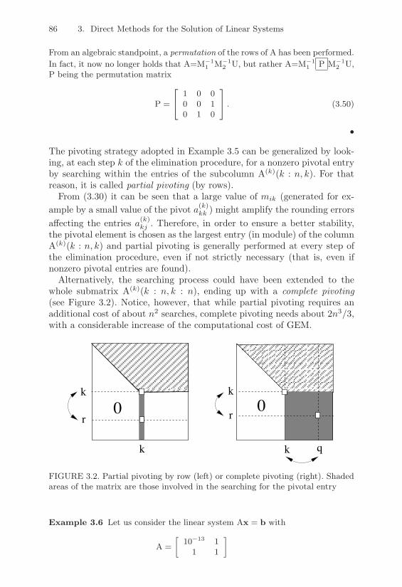
86 3. Direct Methods for the Solution of Linear Systems
From an algebraic standpoint, a permutation of the rows of A has been performed.In fact, it now no longer holds that A=M%1
1 M%12 U, but rather A=M%1
1 P M%12 U,
P being the permutation matrix
P =
"
$1 0 00 0 10 1 0
%
' . (3.50)
•
The pivoting strategy adopted in Example 3.5 can be generalized by look-ing, at each step k of the elimination procedure, for a nonzero pivotal entryby searching within the entries of the subcolumn A(k)(k : n, k). For thatreason, it is called partial pivoting (by rows).
From (3.30) it can be seen that a large value of mik (generated for ex-ample by a small value of the pivot a(k)
kk ) might amplify the rounding errorsa!ecting the entries a(k)
kj . Therefore, in order to ensure a better stability,the pivotal element is chosen as the largest entry (in module) of the columnA(k)(k : n, k) and partial pivoting is generally performed at every step ofthe elimination procedure, even if not strictly necessary (that is, even ifnonzero pivotal entries are found).
Alternatively, the searching process could have been extended to thewhole submatrix A(k)(k : n, k : n), ending up with a complete pivoting(see Figure 3.2). Notice, however, that while partial pivoting requires anadditional cost of about n2 searches, complete pivoting needs about 2n3/3,with a considerable increase of the computational cost of GEM.
0r
k
r
k q
k
k
0
FIGURE 3.2. Partial pivoting by row (left) or complete pivoting (right). Shadedareas of the matrix are those involved in the searching for the pivotal entry
Example 3.6 Let us consider the linear system Ax = b with
A =-
10%13 11 1
.

3.5 Pivoting 87
and where b is chosen in such a way that x = (1, 1)T is the exact solution.Suppose we use base 2 and 16 significant digits. GEM without pivoting wouldgive xMEG = (0.99920072216264, 1)T , while GEM plus partial pivoting furnishesthe exact solution up to the 16th digit. •
Let us analyze how partial pivoting a!ects the LU factorization inducedby GEM. At the first step of GEM with partial pivoting, after findingout the entry ar1 of maximum module in the first column, the elementarypermutation matrix P1 which exchanges the first row with the r-th row isconstructed (if r = 1, P1 is the identity matrix). Next, the first Gaussiantransformation matrix M1 is generated and we set A(2) = M1P1A(1). Asimilar approach is now taken on A(2), searching for a new permutationmatrix P2 and a new matrix M2 such that
A(3) = M2P2A(2) = M2P2M1P1A(1).
Executing all the elimination steps, the resulting upper triangular matrixU is now given by
U = A(n) = Mn"1Pn"1 . . .M1P1A(1). (3.51)
Letting M = Mn"1Pn"1 . . .M1P1 and P = Pn"1 . . .P1, we obtain thatU=MA and, thus, U = (MP"1)PA. It can easily be checked that the matrixL = PM"1 is unit lower triangular, so that the LU factorization reads
PA = LU. (3.52)
One should not be worried by the presence of the inverse of M, since M"1 =P"1
1 M"11 . . .P"1
n"1M"1n"1 and P"1
i = PTi while M"1
i = 2In "Mi.Once L, U and P are available, solving the initial linear system amounts
to solving the triangular systems Ly = Pb and Ux = y. Notice that theentries of the matrix L coincide with the multipliers computed by LU fac-torization, without pivoting, when applied to the matrix PA.If complete pivoting is performed, at the first step of the process, once theelement aqr of largest module in submatrix A(1 : n, 1 : n) has been found,we must exchange the first row and column with the q-th row and ther-th column. This generates the matrix P1A(1)Q1, where P1 and Q1 arepermutation matrices by rows and by columns, respectively.
As a consequence, the action of matrix M1 is now such that A(2) =M1P1A(1)Q1. Repeating the process, at the last step, instead of (3.51) weobtain
U = A(n) = Mn"1Pn"1 . . .M1P1A(1)Q1 . . .Qn"1.
In the case of complete pivoting the LU factorization becomes
PAQ = LU,

88 3. Direct Methods for the Solution of Linear Systems
where Q = Q1 . . .Qn"1 is a permutation matrix accounting for all permu-tations that have been operated. By construction, matrix L is still lowertriangular, with module entries less than or equal to 1. As happens inpartial pivoting, the entries of L are the multipliers produced by the LUfactorization process without pivoting, when applied to the matrix PAQ.
Program 9 is an implementation of the LU factorization with completepivoting. For an e"cient computer implementation of the LU factorizationwith partial pivoting, we refer to the MATLAB intrinsic function lu.
Program 9 - LUpivtot : LU factorization with complete pivoting
function [L,U,P,Q] = LUpivtot(A,n)P=eye(n); Q=P; Minv=P;for k=1:n-1[Pk,Qk]=pivot(A,k,n); A=Pk*A*Qk;[Mk,Mkinv]=MGauss(A,k,n);A=Mk*A; P=Pk*P; Q=Q*Qk;Minv=Minv*Pk*Mkinv;
endU=triu(A); L=P*Minv;
function [Mk,Mkinv]=MGauss(A,k,n)Mk=eye(n);for i=k+1:n, Mk(i,k)=-A(i,k)/A(k,k); endMkinv=2*eye(n)-Mk;
function [Pk,Qk]=pivot(A,k,n)[y,i]=max(abs(A(k:n,k:n))); [piv,jpiv]=max(y);ipiv=i(jpiv); jpiv=jpiv+k-1; ipiv=ipiv+k-1;Pk=eye(n); Pk(ipiv,ipiv)=0; Pk(k,k)=0; Pk(k,ipiv)=1; Pk(ipiv,k)=1;Qk=eye(n); Qk(jpiv,jpiv)=0; Qk(k,k)=0; Qk(k,jpiv)=1; Qk(jpiv,k)=1;
Remark 3.3 The presence of large pivotal entries is not in itself su"cientto guarantee accurate solutions, as demonstrated by the following example(taken from [JM92]). For the linear system Ax = b
"
$"4000 2000 2000
2000 0.78125 02000 0 0
%
'
"
$x1x2x3
%
' =
"
$400
1.38161.9273
%
'
at the first step the pivotal entry coincides with the diagonal entry "4000itself. However, executing GEM on such a matrix yields the solution
:x = [0.00096365, "0.698496, 0.90042329]T
whose first component drastically di!ers from that of the exact solutionx = [1.9273, "0.698496, 0.9004233]T . The cause of this behaviour should
3.6 Computing the Inverse of a Matrix 89
be ascribed to the wide variations among the system coe"cients. Such casescan be remedied by a suitable scaling of the matrix (see Section 3.12.1). !
Remark 3.4 (Pivoting for symmetric matrices) As already noticed,pivoting is not strictly necessary if A is symmetric and positive definite.A separate comment is deserved when A is symmetric but not positivedefinite, since pivoting could destroy the symmetry of the matrix. Thiscan be avoided by employing a complete pivoting of the form PAPT , eventhough this pivoting can only turn out into a reordering of the diagonalentries of A. As a consequence, the presence on the diagonal of A of smallentries might inhibit the advantages of the pivoting. To deal with matricesof this kind, special algorithms are needed (like the Parlett-Reid method[PR70] or the Aasen method [Aas71]) for whose description we refer to[GL89], and to [JM92] for the case of sparse matrices. !
3.6 Computing the Inverse of a Matrix
The explicit computation of the inverse of a matrix can be carried out usingthe LU factorization as follows. Denoting by X the inverse of a nonsingularmatrix A! Rn!n, the column vectors of X are the solutions to the linearsystems Axi = ei, for i = 1, . . . , n.
Supposing that PA=LU, where P is the partial pivoting permutationmatrix, we must solve 2n triangular systems of the form
Lyi = Pei, Uxi = yi i = 1, . . . , n,
i.e., a succession of linear systems having the same coe"cient matrix butdi!erent right hand sides. The computation of the inverse of a matrix is acostly procedure which can sometimes be even less stable than MEG (see[Hig88]).
An alternative approach for computing the inverse of A is provided bythe Faddev or Leverrier formula, which, letting B0=I, recursively computes
"k =1k
tr(ABk"1), Bk = "ABk"1 + "kI, k = 1, 2, . . . , n.
Since Bn = 0, if "n '= 0 we get
A"1 =1"n
Bn"1,
and the computational cost of the method for a full matrix is equal to(n" 1)n3 flops (for further details see [FF63], [Bar89]).

90 3. Direct Methods for the Solution of Linear Systems
3.7 Banded Systems
Discretization methods for boundary value problems often lead to solvinglinear systems with matrices having banded, block or sparse forms. Ex-ploiting the structure of the matrix allows for a dramatic reduction in thecomputational costs of the factorization and of the substitution algorithms.In the present and forthcoming sections, we shall address special variantsof MEG or LU factorization that are properly devised for dealing with ma-trices of this kind. For the proofs and a more comprehensive treatment, werefer to [GL89] and [Hig88] for banded or block matrices, while we refer to[JM92], [GL81] and [Saa96] for sparse matrices and the techniques for theirstorage.
The main result for banded matrices is the following.
Property 3.4 Let A! Rn!n. Suppose that there exists a LU factorizationof A. If A has upper bandwidth q and lower bandwidth p, then L has lowerbandwidth p and U has upper bandwidth q.
In particular, notice that the same memory area used for A is enough toalso store its LU factorization. Consider, indeed, that a matrix A havingupper bandwidth q and lower bandwidth p is usually stored in a matrix B(p + q + 1)% n, assuming that
bi"j+q+1,j = aij
for all the indices i, j that fall into the band of the matrix. For instance, inthe case of the tridiagonal matrix A=tridiag5("1, 2,"1) (where q = p = 1),the compact storage reads
B =
"
$0 "1 "1 "1 "12 2 2 2 2"1 "1 "1 "1 0
%
' .
The same format can be used for storing the factorization LU of A. It isclear that this storage format can be quite inconvenient in the case whereonly a few bands of the matrix are large. In the limit, if only one columnand one row were full, we would have p = q = n and thus B would be afull matrix with a lot of zero entries.
Finally, we notice that the inverse of a banded matrix is generally full(as happens for the matrix A considered above).

3.7 Banded Systems 91
3.7.1 Tridiagonal MatricesConsider the particular case of a linear system with nonsingular tridiagonalmatrix A given by
A =
"
#####$
a1 c1 0b2 a2
. . .. . . cn"1
0 bn an
%
&&&&&'.
In such an event, the matrices L and U of the LU factorization of A arebidiagonal matrices of the form
L =
"
####$
1 0#2 1
. . . . . .0 #n 1
%
&&&&'U =
"
#####$
"1 c1 0"2
. . .
. . . cn"1
0 "n
%
&&&&&'.
The coe"cients "i and #i can easily be computed by the following relations
"1 = a1, #i =bi"i"1
, "i = ai " #ici"1, i = 2, . . . , n. (3.53)
This is known as the Thomas algorithm and can be regarded as a particularinstance of the Doolittle factorization, without pivoting. When one is notinterested in storing the coe"cients of the original matrix, the entries "i
and #i can be overwritten on A.The Thomas algorithm can also be extended to solve the whole tridi-
agonal system Ax = f . This amounts to solving two bidiagonal systemsLy = f and Ux = y, for which the following formulae hold
(Ly = f) y1 = f1, yi = fi " #iyi"1, i = 2, . . . , n, (3.54)
(Ux = y) xn =yn"n
, xi = (yi " cixi+1) /"i, i = n" 1, . . . , 1. (3.55)
The algorithm requires only 8n " 7 flops: precisely, 3(n " 1) flops for thefactorization (3.53) and 5n" 4 flops for the substitution procedure (3.54)-(3.55).
As for the stability of the method, if A is a nonsingular tridiagonal matrixand :L and :U are the factors actually computed, then
|%A| & (4u + 3u2 + u3)|:L| |:U|,

92 3. Direct Methods for the Solution of Linear Systems
where %A is implicitly defined by the relation A + %A = :L:U while u is theroundo! unit. In particular, if A is also symmetric and positive definite orit is an M-matrix, we have
|%A| & 4u + 3u2 + u3
1" u|A|,
which implies the stability of the factorization procedure in such cases. Asimilar result holds even if A is diagonally dominant.
3.7.2 Implementation IssuesAn implementation of the LU factorization for banded matrices is shownin Program 10.
Program 10 - lu band : LU factorization for a banded matrix
function [A] = lu band (A,p,q)[n,n]=size(A);for k = 1:n-1for i = k+1:min(k+p,n), A(i,k)=A(i,k)/A(k,k); endfor j = k+1:min(k+q,n)for i = k+1:min(k+p,n), A(i,j)=A(i,j)-A(i,k)*A(k,j); endendend
In the case where n 4 p and n 4 q, this algorithm approximately takes2npq flops, with a considerable saving with respect to the case in which Ais a full matrix.
Similarly, ad hoc versions of the substitution methods can be devised(see Programs 11 and 12). Their costs are, respectively, of the order of 2npflops and 2nq flops, always assuming that n4 p and n4 q.
Program 11 - forw band : Forward substitution for a banded matrix L
function [b] = forw band (L, p, b)[n,n]=size(L);for j = 1:n
for i=j+1:min(j+p,n); b(i) = b(i) - L(i,j)*b(j); endend
Program 12 - back band : Backward substitution for a banded matrix U
function [b] = back band (U, q, b)[n,n]=size(U);for j=n:-1:1
b (j) = b (j) / U (j,j);for i = max(1,j-q):j-1, b(i)=b(i)-U(i,j)*b(j); end
end
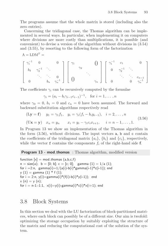
3.8 Block Systems 93
The programs assume that the whole matrix is stored (including also thezero entries).
Concerning the tridiagonal case, the Thomas algorithm can be imple-mented in several ways. In particular, when implementing it on computerswhere divisions are more costly than multiplications, it is possible (andconvenient) to devise a version of the algorithm without divisions in (3.54)and (3.55), by resorting to the following form of the factorizationA = LDMT =
"
####$
,%11 0 0
b2 ,%12
. . .. . .
. . . 00 bn ,%1
n
%
&&&&'
"
####$
,1 0,2
. . .
0 ,n
%
&&&&'
"
####$
,%11 c1 0
0 ,%12
. . .. . .
. . . cn%1
0 0 ,%1n
%
&&&&'
The coe"cients 'i can be recursively computed by the formulae
'i = (ai " bi'i"1ci"1)"1, for i = 1, . . . , n
where '0 = 0, b1 = 0 and cn = 0 have been assumed. The forward andbackward substitution algorithms respectively read
(Ly = f) y1 = '1f1, yi = 'i(fi " biyi"1), i = 2, . . . , n
(Ux = y) xn = yn xi = yi " 'icixi+1, i = n" 1, . . . , 1.(3.56)
In Program 13 we show an implementation of the Thomas algorithm inthe form (3.56), without divisions. The input vectors a, b and c containthe coe"cients of the tridiagonal matrix {ai}, {bi} and {ci}, respectively,while the vector f contains the components fi of the right-hand side f.
Program 13 - mod thomas : Thomas algorithm, modified version
function [x] = mod thomas (a,b,c,f)n = size(a); b = [0; b]; c = [c; 0]; gamma (1) = 1/a (1);for i =2:n, gamma(i)=1/(a(i)-b(i)*gamma(i-1)*c(i-1)); endy (1) = gamma (1) * f (1);for i = 2:n, y(i)=gamma(i)*(f(i)-b(i)*y(i-1)); endx (n) = y (n);for i = n-1:-1:1, x(i)=y(i)-gamma(i)*c(i)*x(i+1); end
3.8 Block Systems
In this section we deal with the LU factorization of block-partitioned matri-ces, where each block can possibly be of a di!erent size. Our aim is twofold:optimizing the storage occupation by suitably exploiting the structure ofthe matrix and reducing the computational cost of the solution of the sys-tem.

94 3. Direct Methods for the Solution of Linear Systems
3.8.1 Block LU FactorizationLet A! Rn!n be the following block partitioned matrix
A =-
A11 A12A21 A22
.,
where A11 ! Rr!r is a nonsingular square matrix whose factorizationL11D1R11 is known, while A22 ! R(n"r)!(n"r). In such a case it is possibleto factorize A using only the LU factorization of the block A11. Indeed, itis true that
-A11 A12A21 A22
.=
-L11 0L21 In"r
. -D1 00 #2
. -R11 R120 In"r
.,
where
L21 = A21R"111 D"1
1 , R12 = D"11 L"1
11 A12,
#2 = A22 " L21D1R12.
If necessary, the reduction procedure can be repeated on the matrix #2,thus obtaining a block-version of the LU factorization.
If A11 were a scalar, the above approach would reduce by one the size ofthe factorization of a given matrix. Applying iteratively this method yieldsan alternative way of performing the Gauss elimination.
We also notice that the proof of Theorem 3.4 can be extended to thecase of block matrices, obtaining the following result.
Theorem 3.7 Let A ! Rn!n be partitioned in m % m blocks Aij withi, j = 1, . . . ,m. A admits a unique LU block factorization (with L havingunit diagonal entries) i! the m " 1 dominant principal block minors of Aare nonzero.
Since the block factorization is an equivalent formulation of the standardLU factorization of A, the stability analysis carried out for the latter holdsfor its block-version as well. Improved results concerning the e"cient usein block algorithms of fast forms of matrix-matrix product are dealt within [Hig88]. In the forthcoming section we focus solely on block-tridiagonalmatrices.
3.8.2 Inverse of a Block-partitioned MatrixThe inverse of a block matrix can be constructed using the LU factorizationintroduced in the previous section. A remarkable application is when A isa block matrix of the form
A = C + UBV,

3.8 Block Systems 95
where C is a block matrix that is “easy” to invert (for instance, when Cis given by the diagonal blocks of A), while U, B and V take into accountthe connections between the diagonal blocks. In such an event A can beinverted by using the Sherman-Morrison or Woodbury formula
A"1 = (C + UBV)"1 = C"1 " C"1U8I + BVC"1U
9"1 BVC"1, (3.57)
having assumed that C and I + BVC"1U are two nonsingular matrices.This formula has several practical and theoretical applications, and is par-ticularly e!ective if connections between blocks are of modest relevance.
3.8.3 Block Tridiagonal SystemsConsider block tridiagonal systems of the form
Anx =
"
#####$
A11 A12 0A21 A22
. . .. . . . . . An"1,n
0 An,n"1 Ann
%
&&&&&'
"
####$
x1......
xn
%
&&&&'=
"
####$
b1......
bn
%
&&&&', (3.58)
where Aij are matrices of order ni%nj and xi and bi are column vectors ofsize ni, for i, j = 1, . . . , n. We assume that the diagonal blocks are squared,although not necessarily of the same size. For k = 1, . . . , n, set
Ak =
"
####$
In1 0L1 In2
. . . . . .0 Lk"1 Ink
%
&&&&'
"
#####$
U1 A12 0U2
. . .
. . . Ak"1,k
0 Uk
%
&&&&&'.
Equating for k = n the matrix above with the corresponding blocks of An,it turns out that U1 = A11, while the remaining blocks can be obtainedsolving sequentially, for i = 2, . . . , n, the systems Li"1Ui"1 = Ai,i"1 forthe columns of L and computing Ui = Aii " Li"1Ai"1,i.This procedure is well defined only if all the matrices Ui are nonsingular,which is the case if, for instance, the matrices A1, . . . ,An are nonsingular.As an alternative, one could resort to factorization methods for bandedmatrices, even if this requires the storage of a large number of zero entries(unless a suitable reordering of the rows of the matrix is performed).
A remarkable instance is when the matrix is block tridiagonal and sym-metric, with symmetric and positive definite blocks. In such a case (3.58)

96 3. Direct Methods for the Solution of Linear Systems
takes the form"
#####$
A11 AT21 0
A21 A22. . .
. . . . . . ATn,n"1
0 An,n"1 Ann
%
&&&&&'
"
####$
x1......
xn
%
&&&&'=
"
####$
b1......
bn
%
&&&&'.
Here we consider an extension to the block case of the Thomas algorithm,which aims at transforming A into a block bidiagonal matrix. To this pur-pose, we first have to eliminate the block corresponding to matrix A21.Assume that the Cholesky factorization of A11 is available and denote byH11 the Cholesky factor. If we multiply the first row of the block systemby H"T
11 , we find
H11x1 + H"T11 AT
21x2 = H"T11 b1.
Letting H21 = H"T11 AT
21 and c1 = H11b1, it follows that A21 = HT21H11 and
thus the first two rows of the system are
H11x1 + H21x2 = c1,
HT21H11x1 + A22x2 + AT
32x3 = b2.
As a consequence, multiplying the first row by HT21 and subtracting it from
the second one, the unknown x1 is eliminated and the following equivalentequation is obtained
A(1)22 x2 + AT
32x3 = b2 "H21c1,
with A(1)22 = A22"HT
21H21. At this point, the factorization of A(1)22 is carried
out and the unknown x3 is eliminated from the third row of the system,and the same is repeated for the remaining rows of the system. At the endof the procedure, which requires solving (n" 1)
!n"1j=1 nj linear systems to
compute the matrices Hi+1,i, i = 1, . . . , n"1, we end up with the followingblock bidiagonal system
"
#####$
H11 H21 0H22
. . .
. . . Hn,n"1
0 Hnn
%
&&&&&'
"
####$
x1......
xn
%
&&&&'=
"
####$
c1......
cn
%
&&&&'
which can be solved with a (block) back substitution method. If all blockshave the same size p, then the number of multiplications required by thealgorithm is about (7/6)(n"1)p3 flops (assuming both p and n very large).
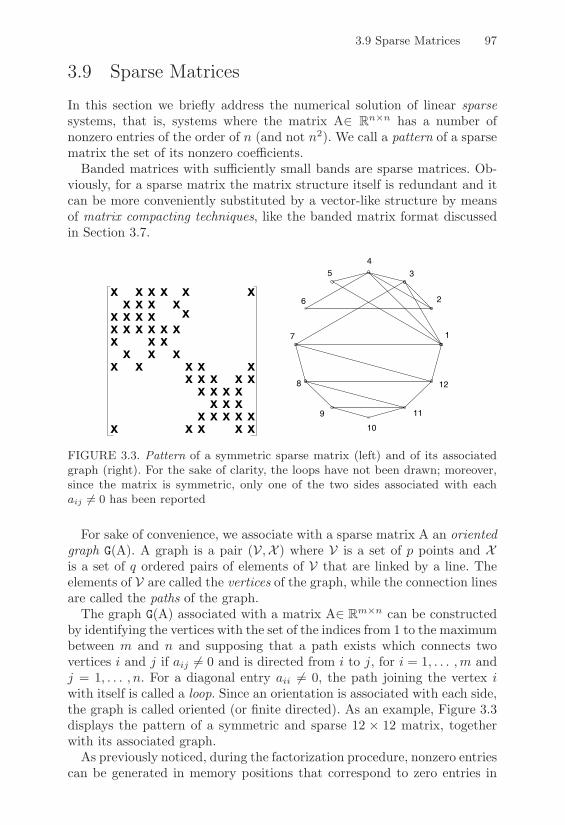
3.9 Sparse Matrices 97
3.9 Sparse Matrices
In this section we briefly address the numerical solution of linear sparsesystems, that is, systems where the matrix A! Rn!n has a number ofnonzero entries of the order of n (and not n2). We call a pattern of a sparsematrix the set of its nonzero coe"cients.
Banded matrices with su"ciently small bands are sparse matrices. Ob-viously, for a sparse matrix the matrix structure itself is redundant and itcan be more conveniently substituted by a vector-like structure by meansof matrix compacting techniques, like the banded matrix format discussedin Section 3.7.
x xx x x xx x x
x x x xx x
x x xx xx x x x
x x x
x
xx xxxx
xxxx
x x x x
x xx xx
x x xxx
xx
1
2
34
5
6
7
8
9
10
11
12
FIGURE 3.3. Pattern of a symmetric sparse matrix (left) and of its associatedgraph (right). For the sake of clarity, the loops have not been drawn; moreover,since the matrix is symmetric, only one of the two sides associated with eachaij $= 0 has been reported
For sake of convenience, we associate with a sparse matrix A an orientedgraph G(A). A graph is a pair (V,X ) where V is a set of p points and Xis a set of q ordered pairs of elements of V that are linked by a line. Theelements of V are called the vertices of the graph, while the connection linesare called the paths of the graph.
The graph G(A) associated with a matrix A! Rm!n can be constructedby identifying the vertices with the set of the indices from 1 to the maximumbetween m and n and supposing that a path exists which connects twovertices i and j if aij '= 0 and is directed from i to j, for i = 1, . . . ,m andj = 1, . . . , n. For a diagonal entry aii '= 0, the path joining the vertex iwith itself is called a loop. Since an orientation is associated with each side,the graph is called oriented (or finite directed). As an example, Figure 3.3displays the pattern of a symmetric and sparse 12 % 12 matrix, togetherwith its associated graph.
As previously noticed, during the factorization procedure, nonzero entriescan be generated in memory positions that correspond to zero entries in
98 3. Direct Methods for the Solution of Linear Systems
the starting matrix. This action is referred to as fill-in. Figure 3.4 shows thee!ect of fill-in on the sparse matrix whose pattern is shown in Figure 3.3.Since use of pivoting in the factorization process makes things even morecomplicated, we shall only consider the case of symmetric positive definitematrices for which pivoting is not necessary.
A first remarkable result concerns the amount of fill-in. Let mi(A) =i " min {j < i : aij '= 0} and denote by E(A) the convex hull of A, givenby
E(A) = {(i, j) : 0 < i" j & mi(A)} . (3.59)
For a symmetric positive definite matrix,
E(A) = E(H + HT ) (3.60)
where H is the Cholesky factor, so that fill-in is confined within the convexhull of A (see Figure 3.4). Moreover, if we denote by lk(A) the number ofactive rows at the k-th step of the factorization (i.e., the number of rowsof A with i > k and aik '= 0), the computational cost of the factorizationprocess is
12
n(
k=1
lk(A) (lk(A) + 3) flops, (3.61)
having accounted for all the nonzero entries of the convex hull. Confinementof fill-in within E(A) ensures that the LU factorization of A can be storedwithout extra memory areas simply by storing all the entries of E(A) (in-cluding the null elements). However, such a procedure might still be highlyine"cient due to the large number of zero entries in the hull (see Exercise11).
On the other hand, from (3.60) one gets that the reduction in the convexhull reflects a reduction of fill-in, and in turn, due to (3.61), of the numberof operations needed to perform the factorization. For this reason severalstrategies for reordering the graph of the matrix have been devised. Amongthem, we recall the Cuthill-McKee method, which will be addressed in thenext section.
An alternative consists of decomposing the matrix into sparse subma-trices, with the aim of reducing the original problem to the solution ofsubproblems of reduced size, where matrices can be stored in full format.This approach leads to submatrix decomposition methods which will beaddressed in Section 3.9.2.
3.9.1 The Cuthill-McKee AlgorithmThe Cuthill-McKee algorithm is a simple and e!ective method for reorder-ing the system variables.

3.9 Sparse Matrices 99
xxx x
x xx x
x x xxx
x
xx x
xx
xxxx
xx
xx xx
x x
xx
x xx x x xx x x
x x x xx x
x x
x
xx xx x x x
x x xxx x
xxx
xxxx
x x x x
x xx xx
x x xxx
xx
FIGURE 3.4. The shaded regions in the left figure show the areas of the matrixthat can be a"ected by fill-in, for the matrix considered in Figure 3.3. Solidlines denote the boundary of E(A). The right figure displays the factors thathave been actually computed. Black dots denote the elements of A that wereoriginarily equal to zero
The first step of the algorithm consists of associating with each vertex ofthe graph the number of its connections with neighboring vertices, calledthe degree of the vertex. Next, the following steps are taken:
1. a vertex with a low number of connections is chosen as the first vertexof the graph;
2. the vertices connected to it are progressively re-labeled starting fromthose having lower degrees;
3. the procedure is repeated starting from the vertices connected to thesecond vertex in the updated list. The nodes already re-labeled areignored. Then, a third new vertex is considered, and so on, until allthe vertices have been explored.
The usual way to improve the e"ciency of the algorithm is based on theso-called reverse form of the Cuthill-McKee method. This consists of ex-ecuting the Cuthill-McKee algorithm described above where, at the end,the i-th vertex is moved into the n " i + 1-th position of the list, n beingthe number of nodes in the graph. Figure 3.5 reports, for comparison, thegraphs obtained using the direct and reverse Cuthill-McKee reordering inthe case of the matrix pattern represented in Figure 3.3, while in Figure3.6 the factors L and U are compared. Notice the absence of fill-in whenthe reverse Cuthill-McKee method is used.
Remark 3.5 For an e"cient solution of linear systems with sparse ma-trices, we mention the public domain libraries SPARSKIT [Saa90], UMF-PACK [DD95] and the MATLAB sparfun package. !

100 3. Direct Methods for the Solution of Linear Systems
1 (3)
2 (4)
3 (2)4 (5)
5 (6)
6 (1)
7 (12)
8 (8)
9 (10)
10 (9)
11 (11)
12 (7)
1 (10)
2 (9)
3 (11)4 (8)
5 (12)
6 (7)
7 (6)
8 (5)
9 (3)
10 (4)11 (2)
12 (1)
FIGURE 3.5. Reordered graphs using the direct (left) and reverse (right)Cuthill-McKee algorithm. The label of each vertex, before reordering is per-formed, is reported in braces
x xx x x xx x
x xx x
x xx x
x
x x xx x
xx x
xxx
xx
x
xx
x
xxx
xxx
x xx x
x x xx
x xx
xx
x
xx x xx x
x xx x
xx xx x
x xxx x
xxx
x
xx
xx
x
xx
x
xx
x
x xxx
xx
x x x xx x x
x xx
xxx
FIGURE 3.6. Factors L and U after the direct (left) and reverse (right)Cuthill-McKee reordering. In the second case, fill-in is absent
3.9.2 Decomposition into SubstructuresThese methods have been developed in the framework of numerical ap-proximation of partial di!erential equations. Their basic strategy consistsof splitting the solution of the original linear system into subsystems ofsmaller size which are almost independent from each other and can beeasily interpreted as a reordering technique.
We describe the methods on a special example, referring for a morecomprehensive presentation to [BSG96]. Consider the linear system Ax=b,where A is a symmetric positive definite matrix whose pattern is shown inFigure 3.3. To help develop an intuitive understanding of the method, wedraw the graph of A in the form as in Figure 3.7.

3.9 Sparse Matrices 101
We then partition the graph of A into the two subgraphs (or substruc-tures) identified in the figure and denote by xk, k = 1, 2, the vectors of theunknowns relative to the nodes that belong to the interior of the k-th sub-structure. We also denote by x3 the vector of the unknowns that lie alongthe interface between the two substructures. Referring to the decomposi-tion in Figure 3.7, we have x1 = (2, 3, 4, 6)T , x2 = (8, 9, 10, 11, 12)T
and x3 = (1, 5, 7)T .As a result of the decomposition of the unknowns, matrix A will be
partitioned in blocks, so that the linear system can be written in the form
substructure II
6
7
3
2
4
5 1
12
8 9
11 10
substructure I
FIGURE 3.7. Decomposition into two substructures
"
$A11 0 A130 A22 A23AT
13 AT23 A33
%
'
"
$x1x2x3
%
' =
"
$b1b2b3
%
' ,
having reordered the unknowns and partitioned accordingly the right handside of the system. Suppose that A33 is decomposed into two parts, A*
33and A**
33, which represent the contributions to A33 of each substructure.Similarly, let the right hand side b3 be decomposed as b*
3+b**3 . The original
linear system is now equivalent to the following pair-
A11 A13AT
13 A*33
. -x1x3
.=
-b1b*
3 + #3
.,
-A22 A23AT
23 A**33
. -x2x3
.=
-b2b**
3 " #3
.
having denoted by #3 a vector that takes into account the coupling betweenthe substructures. A typical way of proceeding in decomposition techniquesconsists of eliminating #3 to end up with independent systems, one for each

102 3. Direct Methods for the Solution of Linear Systems
substructure. Let us apply this strategy to the example at hand. The linearsystem for the first substructure is
-A11 A13AT
13 A*33
. -x1x3
.=
-b1b*
3 + #3
.. (3.62)
Let us now factorize A11 as HT11H11 and proceed with the reduction method
already described in Section 3.8.3 for block tridiagonal matrices. We obtainthe system
-H11 H210 A*
33 "H21HT21
. -x1x3
.=
-c1b*
3 + #3 "H21c1
.
where H21 = H"T11 A13 and c1 = H"T
11 b1. The second equation of this systemyields #3 explicitly as
#3 =8A*
33 "HT21H21
9x3 " b*
3 + HT21c1.
Substituting this equation into the system for the second substructure, oneends up with a system only in the unknowns x2 and x3
-A22 A23AT
23 A***33
. -x2x3
.=
-b2b***
3
., (3.63)
where A***33 = A33 " HT
21H21 and b***3 = b3 " HT
21c1. Once (3.63) has beensolved, it will be possible, by backsubstitution into (3.62), to compute alsox1.
The technique described above can be easily extended to the case ofseveral substructures and its e"ciency will increase the more the substruc-tures are mutually independent. It reproduces in nuce the so-called frontalmethod (introduced by Irons [Iro70]), which is quite popular in the solutionof finite element systems (for an implementation, we refer to the UMF-PACK library [DD95]).
Remark 3.6 (The Schur complement) An approach that is dual tothe above method consists of reducing the starting system to a systemacting only on the interface unknowns x3, passing through the assemblingof the Schur complement of matrix A, defined in the 3%3 case at hand as
S = A33 "AT13A
"111 A13 "AT
23A"122 A23.
The original problem is thus equivalent to the system
Sx3 = b3 "AT13A
"111 b1 "AT
23A"122 b2.
This system is full (even if the matrices Aij were sparse) and can be solvedusing either a direct or an iterative method, provided that a suitable pre-conditioner is available. Once x3 has been computed, one can get x1 and

3.10 Accuracy of the Solution Achieved Using GEM 103
x2 by solving two systems of reduced size, whose matrices are A11 and A22,respectively.
We also notice that if the block matrix A is symmetric and positivedefinite, then the linear system on the Schur complement S is no moreill-conditioned than the original system on A, since
K2(S) & K2(A)
(for a proof, see Lemma 3.12, [Axe94]. See also [CM94] and [QV99]). !
3.9.3 Nested DissectionThis is a renumbering technique quite similar to substructuring. In practice,it consists of repeating the decomposition process several times at eachsubstructure level, until the size of each single block is made su"cientlysmall. In Figure 3.8 a possible nested dissection is shown in the case of thematrix considered in the previous section. Once the subdivision procedurehas been completed, the vertices are renumbered starting with the nodesbelonging to the latest substructuring level and moving progressively up tothe first level. In the example at hand, the new node ordering is 11, 9, 7,6, 12, 8, 4, 2, 1, 5, 3.
This procedure is particularly e!ective if the problem has a large size andthe substructures have few connections between them or exhibit a repetitivepattern [Geo73].
3.10 Accuracy of the Solution Achieved UsingGEM
Let us analyze the e!ects of rounding errors on the accuracy of the solutionyielded by GEM. Suppose that A and b are a matrix and a vector offloating-point numbers. Denoting by :L and :U, respectively, the matricesof the LU factorization induced by GEM and computed in floating-pointarithmetic, the solution :x yielded by GEM can be regarded as being thesolution (in exact arithmetic) of the perturbed system (A + %A):x = b,where %A is a perturbation matrix such that
|%A| & nuK3|A| + 5|:L||:U|
L+ O(u2), (3.64)
where u is the roundo! unit and the matrix absolute value notation hasbeen used (see [GL89], Section 3.4.6). As a consequence, the entries of %Awill be small in size if the entries of :L and :U are small. Using partialpivoting allows for bounding below 1 the module of the entries of :L in sucha way that, passing to the infinity norm and noting that +:L+$ & n, the

104 3. Direct Methods for the Solution of Linear Systems
1
A
2
1
A
A
2
1
2
B
A
6
5
4 3
C
A
4 AC
34C
B
6B
56
53
FIGURE 3.8. Two steps of nested dissection. Graph partitioning (left) and matrixreordering (right)
estimate (3.64) becomes
+%A+$ & nuK3+A+$ + 5n+:U+$
L+ O(u2). (3.65)
The bound for +%A+$ in (3.65) is of practical use only if it is possible toprovide an estimate for +:U+$. With this aim, backward analysis can becarried out introducing the so-called growth factor
)n =maxi,j,k
|:a(k)ij |
maxi,j
|aij |. (3.66)
Taking advantage of the fact that |:uij | & )nmaxi,j
|aij |, the following result
due to Wilkinson can be drawn from (3.65),
+%A+$ & 8un3)n+A+$ + O(u2). (3.67)
The growth factor can be bounded by 2n"1 and, although in most of thecases it is of the order of 10, there exist matrices for which the inequality in(3.67) becomes an equality (see, for instance, Exercise 5). For some specialclasses of matrices, a sharp bound for )n can be found:
3.10 Accuracy of the Solution Achieved Using GEM 105
1. for banded matrices with upper and lower bands equal to p, )n &22p"1 " (p " 1)2p"2. As a consequence, in the tridiagonal case onegets )n & 2;
2. for Hessenberg matrices, )n & n;
3. for symmetric positive definite matrices, )n = 1;
4. for matrices strictly diagonally dominant by columns, )n & 2.
To achieve better stability when using GEM for arbitrary matrices, re-sorting to complete pivoting would seem to be mandatory, since it ensuresthat )n & n1/2 8
2 · 31/2 · . . . · n1/(n"1)91/2. Indeed, this growth is slowerthan 2n"1 as n increases.
However, apart from very special instances, GEM with only partial piv-oting exhibits acceptable growth factors. This make it the most commonlyemployed method in the computational practice.
Example 3.7 Consider the linear system (3.2) with
A =-
& 11 0
., b =
-1 + &
1
., (3.68)
which admits the exact solution x=1 for any value of &. The matrix is well-conditioned, having K!(A) = (1 + &)2. Attempting to solve the system for & =10%15 by the LU factorization with 16 significant digits, and using the Programs5, 2 and 3, yields the solution :x = [0.8881784197001253, 1.000000000000000]T ,with an error greater than 11% on the first component. Some insight into thecauses of the inaccuracy of the computed solution can be drawn from (3.64).Indeed this latter does not provide a uniformly small bound for all the entries ofmatrix !A, rather
|!A| "-
3.55 · 10%30 1.33 · 10%15
1.33 · 10%15 2.22
..
Notice that the entries of the corresponding matrices :L and :U are quite large inmodule. Conversely, resorting to GEM with partial or complete pivoting yieldsthe exact solution of the system (see Exercise 6). •
Let us now address the role of the condition number in the error analysisfor GEM. GEM yields a solution :x that is typically characterized by havinga small residual :r = b" A:x (see [GL89]). This feature, however, does notensure that the error x" :x is small when K(A) 4 1 (see Example 3.8). Infact, if %b in (3.11) is regarded as being the residual, then
+x" :x++x+ & K(A)+:r+ 1
+A++x+ & K(A)+:r++b+ .
This result will be applied to devise methods, based on the a posteriorianalysis, for improving the accuracy of the solution of GEM (see Section3.12).

106 3. Direct Methods for the Solution of Linear Systems
Example 3.8 Consider the linear system Ax = b with
A =-
1 1.00011.0001 1
., b =
-11
.,
which admits the solution x = (0.499975 . . . , 0.499975 . . . )T . Assuming as an ap-proximate solution the vector :x = (%4.499775, 5.5002249)T , one finds the residual:r 0 (%0.001, 0)T , which is small although :x is quite di"erent from the exact so-lution. The reason for this is due to the ill-conditioning of matrix A. Indeed inthis case K!(A) = 20001. •
An estimate of the number of exact significant digits of a numericalsolution of a linear system can be given as follows. From (3.13), letting' = u and assuming that uK$(A) & 1/2 we get
+"x+$+x+$
& 2uK$(A)1" uK$(A)
& 4uK$(A).
As a consequence
+:x" x+$+x+$
1 uK$(A). (3.69)
Assuming that u 1 #"t and K$(A) 1 #m, one gets that the solution :xcomputed by GEM will have at least t"m exact digits, t being the numberof digits available for the mantissa. In other words, the ill-conditioning of asystem depends both on the capability of the floating-point arithmetic thatis being used and on the accuracy that is required in the solution.
3.11 An Approximate Computation of K(A)
Suppose that the linear system (3.2) has been solved by a factorizationmethod. To determine the accuracy of the computed solution, the analy-sis carried out in Section 3.10 can be used if an estimate of the conditionnumber K(A) of A, which we denote by :K(A), is available. Indeed, al-though evaluating +A+ can be an easy task if a suitable norm is chosen(for instance, + · +1 or + · +$), it is by no means reasonable (or compu-tationally convenient) to compute A"1 if the only purpose is to evaluate+A"1+. For this reason, we describe in this section a procedure (proposedin [CMSW79]) that approximates +A"1+ with a computational cost of theorder of n2 flops.
The basic idea of the algorithm is as follows: #d ! Rn with d '= 0, thanksto the definition of matrix norm, +A"1+ ) +y+/+d+ = '(d) with Ay = d.Thus, we look for d in such a way that '(d) is as large as possible andassume the obtained value as an estimate of +A"1+.
For the method to be e!ective, the selection of d is crucial. To explainhow to do this, we start by assuming that the QR factorization of A has

3.11 An Approximate Computation of K(A) 107
been computed and that K2(A) is to be approximated. In such an event,since K2(A) = K2(R) due to Property 1.8, it su"ces to estimate +R"1+2instead of +A"1+2. Considerations related to the SVD of R induce approx-imating +R"1+2 by the following algorithm:
compute the vectors x and y, solutions to the systems
RTx = d, Ry = x, (3.70)
then estimate +R"1+2 by the ratio '2 = +y+2/+x+2. The vector d appearingin (3.70) should be determined in such a way that '2 is as close as possibleto the value actually attained by +R"1+2. It can be shown that, except invery special cases, '2 provides for any choice of d a reasonable (althoughnot very accurate) estimate of +R"1+2 (see Exercise 15). As a consequence,a proper selection of d can encourage this natural trend.
Before going on, it is worth noting that computing K2(R) is not an easymatter even if an estimate of +R"1+2 is available. Indeed, it would remainto compute +R+2 =
3)(RTR). To overcome this di"culty, we consider
henceforth K1(R) instead of K2(R) since +R+1 is easily computable. Then,heuristics allows us to assume that the ratio '1 = +y+1/+x+1 is an estimateof +R"1+1, exactly as '2 is an estimate of +R"1+2.
Let us now deal with the choice of d. Since RTx = d, the generic compo-nent xk of x can be formally related to x1, . . . , xk"1 through the formulaeof forward substitution as
r11x0 = d1,
rkkxk = dk " (r1kx1 + . . . + rk"1,kxk"1), k ) 1.(3.71)
Assume that the components of d are of the form dk = ±!k, where !kare random numbers and set arbitrarily d1 = !1. Then, x1 = !1/r11 iscompletely determined, while x2 = (d2" r12x1)/r22 depends on the sign ofd2. We set the sign of d2 as the opposite of r12x1 in such a way to make+x(1 : 2)+1 = |x1| + |x2|, for a fixed x1, the largest possible. Once x2 isknown, we compute x3 following the same criterion, and so on, until xn.
This approach sets the sign of each component of d and yields a vectorx with a presumably large + · +1. However, it can fail since it is based onthe idea (which is in general not true) that maximizing +x+1 can be doneby selecting at each step k in (3.71) the component xk which guaranteesthe maximum increase of +x(1 : k " 1)+1 (without accounting for the factthat all the components are related).
Therefore, we need to modify the method by including a sort of “look-ahead” strategy, which accounts for the way of choosing dk a!ects all latervalues xi, with i > k, still to be computed. Concerning this point, we noticethat for a generic row i of the system it is always possible to compute at

108 3. Direct Methods for the Solution of Linear Systems
step k the vector p(k"1) with components
p(k"1)i = 0 i = 1, . . . , k " 1,
p(k"1)i = r1ix1 + . . . + rk"1,ixk"1 i = k, . . . , n.
Thus xk = (±!k " p(k"1)k )/rkk. We denote the two possible values of xk by
x+k and x"
k . The choice between them is now taken not only accounting forwhich of the two most increases +x(1 : k)+1, but also evaluating the increaseof +p(k)+1. This second contribution accounts for the e!ect of the choice ofdk on the components that are still to be computed. We can include bothcriteria in a unique test. Denoting by
p(k)+i = 0, p(k)"
i = 0, i = 1, . . . , k,
p(k)+i = p(k"1)
i + rkix+k , p(k)"
i = p(k"1)i + rkix
"k , i = k + 1, . . . , n,
the components of the vectors p(k)+ and p(k)" respectively, we set eachk-th step dk = +!k or dk = "!k according to whether |rkkx+
k | + +p(k)++1is greater or less than |rkkx"
k | + +p(k)"+1.Under this choice d is completely determined and the same holds for x.
Now, solving the system Ry = x, we are warranted that +y+1/+x+1 is a reli-able approximation to +R"1+1, so that we can set :K1(A) = +R+1+y+1/+x+1.
In practice the PA=LU factorization introduced in Section 3.5 is usuallyavailable. Based on the previous considerations and on some heuristics, ananalogous procedure to that shown above can be conveniently employedto approximate +A"1+1. Precisely, instead of systems (3.70), we must nowsolve
(LU)Tx = d, LUy = x.
We set +y+1/+x+1 as the approximation of +A"1+1 and, consequently, wedefine :K1(A). The strategy for selecting d can be the same as before;indeed, solving (LU)Tx = d amounts to solving
UT z = d, LTx = z, (3.72)
and thus, since UT is lower triangular, we can proceed as in the previouscase. A remarkable di!erence concerns the computation of x. Indeed, whilethe matrix RT in the second system of (3.70) has the same condition numberas R, the second system in (3.72) has a matrix LT which could be even moreill-conditioned than UT . If this were the case, solving for x could lead toan inaccurate outcome, thus making the whole process useless.
Fortunately, resorting to partial pivoting prevents this circumstance fromoccurring, ensuring that any ill-condition in A is reflected in a correspond-ing ill-condition in U. Moreover, picking !k randomly between 1/2 and 1

3.12 Improving the Accuracy of GEM 109
guarantees accurate results even in the special cases where L turns out tobe ill-conditioned.
The algorithm presented below is implemented in the LINPACK library[BDMS79] and in the MATLAB function rcond. This function, in orderto avoid rounding errors, returns as output parameter the reciprocal of:K1(A). A more accurate estimator, described in [Hig88], is implemented inthe MATLAB function condest.
Program 14 implements the approximate evaluation of K1 for a matrixA of generic form. The input parameters are the size n of the matrix A, thematrix A, the factors L, U of its PA=LU factorization and the vector thetacontaining the random numbers !k, for k = 1, . . . , n.
Program 14 - cond est : Algorithm for the approximation of K1(A)
function [k1] = cond est(n,A,L,U,theta)for i=1:n, p(i)=0; endfor k=1:nzplus=(theta(k)-p(k))/U(k,k); zminu=(-theta(k)-p(k))/U(k,k);splus=abs(theta(k)-p(k)); sminu=abs(-theta(k)-p(k));for i=(k+1):nsplus=splus+abs(p(i)+U(k,i)*zplus);sminu=sminu+abs(p(i)+U(k,i)*zminu);
endif splus >= sminu, z(k)=zplus; else, z(k)=zminu; endfor i=(k+1):n, p(i)=p(i)+U(k,i)*z(k); end
endz = z’; x = backward col(L’,z);w = forward col(L,x); y = backward col(U,w);k1=norm(A,1)*norm(y,1)/norm(x,1);
Example 3.9 Let us consider the Hilbert matrix H4. Its condition numberK1(H4), computed using the MATLAB function invhilb which returns the exactinverse of H4, is 2.8375 · 104. Running Program 14 with theta=(1, 1, 1, 1)T givesthe reasonable estimate :K1(H4) = 2.1523 · 104 (which is the same as the outputof rcond), while the function condest returns the exact result. •
3.12 Improving the Accuracy of GEM
As previously noted if the matrix of the system is ill-conditioned, the so-lution generated by GEM could be inaccurate even though its residual issmall. In this section, we mention two techniques for improving the accu-racy of the solution computed by GEM.

110 3. Direct Methods for the Solution of Linear Systems
3.12.1 ScalingIf the entries of A vary greatly in size, it is likely that during the eliminationprocess large entries are summed to small entries, with a consequent onsetof rounding errors. A remedy consists of performing a scaling of the matrixA before the elimination is carried out.
Example 3.10 Consider again the matrix A of Remark 3.3. Multiplying it onthe right and on the left with matrix D=diag(0.0005, 1, 1), we obtain the scaledmatrix
A = DAD =
"
$%0.0001 1 1
1 0.78125 01 0 0
%
' .
Applying GEM to the scaled system Ax = Db = (0.2, 1.3816, 1.9273)T , we getthe correct solution x = Dx. •
Row scaling of A amounts to finding a diagonal nonsingular matrix D1such that the diagonal entries of D1A are of the same size. The linearsystem Ax = b transforms into
D1Ax = D1b.
When both rows and columns of A are to be scaled, the scaled version of(3.2) becomes
(D1AD2)y = D1b with y = D"12 x,
having also assumed that D2 is invertible. Matrix D1 scales the equationswhile D2 scales the unknowns. Notice that, to prevent rounding errors, thescaling matrices are chosen in the form
D1 = diag(#r1 , . . . ,#rn), D2 = diag(#c1 , . . . ,#cn),
where # is the base of the used floating-point arithmetic and the exponentsr1, . . . , rn, c1, . . . , cn must be determined. It can be shown that
+D"12 (:x" x)+$+D"1
2 x+$1 uK$(D1AD2).
Therefore, scaling will be e!ective if K$(D1AD2) is much less than K$(A).Finding convenient matrices D1 and D2 is not in general an easy matter.
A strategy consists, for instance, of picking up D1 and D2 in such a waythat +D1AD2+$ and +D1AD2+1 belong to the interval [1/#, 1], where # isthe base of the used floating-point arithmetic (see [McK62] for a detailedanalysis in the case of the Crout factorization).
3.12 Improving the Accuracy of GEM 111
Remark 3.7 (The Skeel condition number) The Skeel condition num-ber, defined as cond(A) = + |A"1| |A| +$, is the supremum over the setx! Rn, with x '= 0, of the numbers
cond(A,x) =+ |A"1| |A| |x| +$
+x+$.
Unlike what happens for K(A), cond(A,x) is invariant with respect to ascaling by rows of A, that is, to transformations of A of the form DA, whereD is a nonsingular diagonal matrix. As a consequence, cond(A) provides asound indication of the ill-conditioning of a matrix, irrespectively of anypossible row diagonal scaling. !
3.12.2 Iterative RefinementIterative refinement is a technique for improving the accuracy of a solutionyielded by a direct method. Suppose that the linear system (3.2) has beensolved by means of LU factorization (with partial or complete pivoting),and denote by x(0) the computed solution. Having fixed an error tolerance,toll, the iterative refinement performs as follows: for i = 0, 1, . . . , untilconvergence:
1. compute the residual r(i) = b"Ax(i);
2. solve the linear system Az = r(i) using the LU factorization of A;
3. update the solution setting x(i+1) = x(i) + z;
4. if +z+/+x(i+1)+ < toll, then terminate the process returning the solu-tion x(i+1). Otherwise, the algorithm restarts at step 1.
In absence of rounding errors, the process would stop at the first step,yielding the exact solution. The convergence properties of the methodcan be improved by computing the residual r(i) in double precision, whilecomputing the other quantities in single precision. We call this proceduremixed-precision iterative refinement (shortly, MPR), as compared to fixed-precision iterative refinement (FPR).
It can be shown that, if + |A"1| |:L| |:U| +$ is su"ciently small, then ateach step i of the algorithm, the relative error +x"x(i)+$/+x+$ is reducedby a factor ), which is given by
) 1 2 n cond(A,x)u (FPR),
) 1 u (MPR),
where ) is independent of the condition number of A in the case of MPR.Slow convergence of FPR is a clear indication of the ill-conditioning of the

112 3. Direct Methods for the Solution of Linear Systems
matrix, as it can be shown that, if p is the number of iterations for themethod to converge, then K$(A) 1 #t(1"1/p).
Even if performed in fixed precision, iterative refinement is worth usingsince it improves the overall stability of any direct method for solving thesystem. We refer to [Ric81], [Ske80], [JW77] [Ste73], [Wil63] and [CMSW79]for an overview of this subject.
3.13 Undetermined Systems
We have seen that the solution of the linear system Ax=b exists and isunique if n = m and A is nonsingular. In this section we give a meaningto the solution of a linear system both in the overdetermined case, wherem > n, and in the underdetermined case, corresponding to m < n. Wenotice that an underdetermined system generally has no solution unlessthe right side b is an element of range(A).For a detailed presentation, we refer to [LH74], [GL89] and [Bjo88].
Given A! Rm!n with m ) n, b! Rm, we say that x, ! Rn is a solutionof the linear system Ax=b in the least-squares sense if
'(x,) = +Ax, " b+22 & minx#Rn
+Ax" b+22 = minx#Rn
'(x). (3.73)
The problem thus consists of minimizing the Euclidean norm of the resid-ual. The solution of (3.73) can be found by imposing the condition that thegradient of the function ' in (3.73) must be equal to zero at x,. From
'(x) = (Ax" b)T (Ax" b) = xTATAx" 2xTATb + bTb,
we find that
5'(x,) = 2ATAx, " 2ATb = 0,
from which it follows that x, must be the solution of the square system
ATAx, = ATb (3.74)
known as the system of normal equations. The system is nonsingular ifA has full rank and in such a case the least-squares solution exists andis unique. We notice that B = ATA is a symmetric and positive definitematrix. Thus, in order to solve the normal equations, one could first com-pute the Cholesky factorization B = HTH and then solve the two systemsHTy = ATb and Hx, = y. However, due to roundo! errors, the com-putation of ATA may be a!ected by a loss of significant digits, with aconsequent loss of positive definiteness or nonsingularity of the matrix, ashappens in the following example (implemented in MATLAB) where for a

3.13 Undetermined Systems 113
matrix A with full rank, the corresponding matrix fl(ATA) turns out tobe singular
A =
"
$1 12"27 00 2"27
%
' , f l(ATA) =-
1 11 1
..
Therefore, in the case of ill-conditioned matrices it is more convenient toutilize the QR factorization introduced in Section 3.4.3. Indeed, the follow-ing result holds.
Theorem 3.8 Let A ! Rm!n, with m ) n, be a full rank matrix. Thenthe unique solution of (3.73) is given by
x, = R"1QTb (3.75)
where R ! Rn!n and Q ! Rm!n are the matrices defined in (3.48) startingfrom the QR factorization of A. Moreover, the minimum of ' is given by
'(x,) =m(
i=n+1
[(QTb)i]2.
Proof. The QR factorization of A exists and is unique since A has full rank.Thus, there exist two matrices, Q/ Rm&m and R/ Rm&n such that A=QR, whereQ is orthogonal. Since orthogonal matrices preserve the Euclidean scalar product(see Property 1.8), it follows that
&Ax% b&22 = &Rx%QTb&22.
Recalling that R is upper trapezoidal, we have
&Rx%QTb&22 = &Rx% QTb&22 +m(
i=n+1
[(QTb)i]2,
so that the minimum is achieved when x = x). !
For more details about the analysis of the computational cost the algo-rithm (which depends on the actual implementation of the QR factoriza-tion), as well as for results about its stability, we refer the reader to thetexts quoted at the beginning of the section.
If A does not have full rank, the solution techniques above fail, since inthis case if x, is a solution to (3.73), the vector x, + z, with z ! ker(A), isa solution too. We must therefore introduce a further constraint to enforcethe uniqueness of the solution. Typically, one requires that x, has minimalEuclidean norm, so that the least-squares problem can be formulated as
find x, ! Rn with minimal Euclidean norm such that
+Ax, " b+22 & minx#Rn
+Ax" b+22.(3.76)

114 3. Direct Methods for the Solution of Linear Systems
This problem is consistent with (3.73) if A has full rank, since in this case(3.73) has a unique solution which necessarily must have minimal Euclideannorm.
The tool for solving (3.76) is the singular value decomposition (or SVD,see Section 1.9), for which the following theorem holds.
Theorem 3.9 Let A ! Rm!n with SVD given by A = U&VT . Then theunique solution to (3.76) is
x, = A†b (3.77)
where A† is the pseudo-inverse of A introduced in Definition 1.15.
Proof. Using the SVD of A, problem (3.76) is equivalent to finding w = VTxsuch that w has minimal Euclidean norm and
&#w %UTb&22 " &#y %UTb&22, )y / Rn.
If r is the number of nonzero singular values 'i of A, then
&#w %UTb&22 =r(
i=1
K'iwi % (UTb)i
L2+
m(
i=r+1
K(UTb)i
L2,
which is minimum if wi = (UTb)i/'i for i = 1, . . . , r. Moreover, it is clear thatamong the vectors w of Rn having the first r components fixed, the one withminimal Euclidean norm has the remaining n % r components equal to zero.Thus the solution vector is w) = #†UTb, that is, x) = V#†UTb = A†b, where#† is the diagonal matrix defined in (1.11). !
As for the stability of problem (3.76), we point out that if the matrixA does not have full rank, the solution x, is not necessarily a continuousfunction of the data, so that small changes on these latter might producelarge variations in x,. An example of this is shown below.
Example 3.11 Consider the system Ax = b with
A =
"
$1 00 00 0
%
' , b =
"
$123
%
' , rank(A) = 1.
Using the MATLAB function svd we can compute the SVD of A. Then computingthe pseudo-inverse, one finds the solution vector x) = (1, 0)T . If we perturb thenull entry a22, with the value 10%12, the perturbed matrix has (full) rank 2and the solution (which is unique in the sense of (3.73)) is now given by :x) =81, 2 · 10129T . •
We refer the reader to Section 5.8.3 for the approximate computation ofthe SVD of a matrix.
3.14 Applications 115
In the case of underdetermined systems, for which m < n, if A has fullrank the QR factorization can still be used. In particular, when appliedto the transpose matrix AT , the method yields the solution of minimaleuclidean norm. If, instead, the matrix has not full rank, one must resortto SVD.
Remark 3.8 If m = n (square system), both SVD and QR factorizationcan be used to solve the linear system Ax=b, as alternatives to GEM.Even though these algorithms require a number of flops far superior toGEM (SVD, for instance, requires 12n3 flops), they turn out to be moreaccurate when the system is ill-conditioned and nearly singular. !
Example 3.12 Compute the solution to the linear system H15x=b, where H15
is the Hilbert matrix of order 15 (see (3.32)) and the right side is chosen insuch a way that the exact solution is the unit vector x = 1. Using GEM withpartial pivoting yields a solution a"ected by a relative error larger than 100%. Asolution of much better quality is obtained by passing through the computationof the pseudo-inverse, where the entries in # that are less than 10%13 are setequal to zero. •
3.14 Applications
In this section we present two problems, suggested by structural mechan-ics and grid generation in finite element analysis, whose solutions requiresolving large linear systems.
3.14.1 Nodal Analysis of a Structured FrameLet us consider a structured frame which is made by rectilinear beams con-nected among them through hinges (referred to as the nodes) and suitablyconstrained to the ground. External loads are assumed to be applied atthe nodes of the frame and for any beam in the frame the internal actionsamount to a unique force of constant strength and directed as the beamitself. If the normal stress acting on the beam is a traction we assumethat it has positive sign, otherwise the action has negative sign. Structuredframes are frequently employed as covering structures for large size publicbuildings like exhibition stands, railway stations or airport halls.
To determine the internal actions in the frame, that are the unknownsof the mathematical problem, a nodal analysis is used (see [Zie77]): theequilibrium with respect to translation is imposed at every node of theframe yielding a sparse and large-size linear system. The resulting matrixhas a sparsity pattern which depends on the numbering of the unknownsand that can strongly a!ect the computational e!ort of the LU factorization

116 3. Direct Methods for the Solution of Linear Systems
due to fill-in. We will show that the fill-in can be dramatically reduced bya suitable reordering of the unknowns.
The structure shown in Figure 3.9 is arc-shaped and is symmetric withrespect to the origin. The radii r and R of the inner and outer circles areequal to 1 and 2, respectively. An external vertical load of unit size directeddownwards is applied at (0, 1) while the frame is constrained to groundthrough a hinge at ("(r + R), 0) and a bogie at (r + R, 0). To generatethe structure we have partitioned the half unit circle in n( uniform slices,resulting in a total number of n = 2(n( + 1) nodes and a matrix size ofm = 2n. The structure in Figure 3.9 has n( = 7 and the unknowns arenumbered following a counterclockwise labeling of the beams starting fromthe node at (1, 0).
We have represented the structure along with the internal actions com-puted by solving the nodal equilibrium equations where the width of thebeams is proportional to the strength of the computed action. Black isused to identify tractions whereas gray is associated with compressions. Asexpected the maximum traction stress is attained at the node where theexternal load is applied.
!2 !1.5 !1 !0.5 0 0.5 1 1.5 2
!0.5
0
0.5
1
1.5
2
2.5
FIGURE 3.9. A structured frame loaded at the point (0, 1)
We show in Figure 3.10 the sparsity pattern of matrix A (left) and thatof the L-factor of its LU factorization with partial pivoting (right) in thecase n( = 40 which corresponds to a size of 164 % 164. Notice the largefill-in e!ect arising in the lower part of L which results in an increase ofthe nonzero entries from 645 (before the factorization) to 1946 (after thefactorization).

3.14 Applications 117
0 20 40 60 80 100 120 140 160
0
20
40
60
80
100
120
140
160
nz = 6450 20 40 60 80 100 120 140 160
0
20
40
60
80
100
120
140
160
nz = 1946
FIGURE 3.10. Sparsity pattern of matrix A (left) and of the L-factor of the LUfactorization with partial pivoting (right) in the case n# = 40
In view of the solution of the linear system by a direct method, theincrease of the nonzero entries demands for a suitable reordering of theunknowns. For this purpose we use the MATLAB function symrcm whichimplements the symmetric reverse Cuthill-McKee algorithm described inSection 3.9.1. The sparsity pattern, after reordering, is shown in Figure 3.11(left) while the L-factor of the LU factorization of the reordered matrixis shown in Figure 3.11 (right). The results indicate that the reorderingprocedure has “scattered” the sparsity pattern throughout the matrix witha relatively modest increase of the nonzero entries from 645 to 1040.
0 20 40 60 80 100 120 140 160
0
20
40
60
80
100
120
140
160
nz = 6450 20 40 60 80 100 120 140 160
0
20
40
60
80
100
120
140
160
nz = 1040
FIGURE 3.11. Sparsity pattern of matrix A (left) after a reordering with the sym-metric reverse Cuthill-McKee algorithm and the L-factor of the LU factorizationof the reordered matrix with partial pivoting (right) in the case n# = 40
The e!ectiveness of the symmetric reverse Cuthill-McKee reordering pro-cedure is demonstrated in Figure 3.12 which shows the number of nonzeroentries nz in the L-factor of A as a function of the size m of the matrix(represented on the x-axis). In the reordered case (solid line) a linear in-

118 3. Direct Methods for the Solution of Linear Systems
crease of nz with m can be clearly appreciated at the expense of a dramaticfill-in growing with m if no reordering is performed (dashed line).
0 100 200 300 400 500 600 700 800 900 10000
1
2
3
4
5
6x 10
4
FIGURE 3.12. Number of nonzero entries in the L-factor of A as a function ofthe size m of the matrix, with (solid line) and without (dashed line) reordering
3.14.2 Regularization of a Triangular GridThe numerical solution of a problem in a two-dimensional domain D ofpolygonal form, for instance by finite element or finite di!erence methods,very often requires that D be decomposed in smaller subdomains, usuallyof triangular form (see for instance Section 9.9.2).
Suppose that D =M
T#Th
T , where Th is the considered triangulation (also
called computational grid) and h is a positive parameter which characterizesthe triangulation. Typically, h denotes the maximum length of the triangleedges. We shall also assume that two triangles of the grid, T1 and T2, haveeither null intersection or share a vertex or a side.The geometrical properties of the computational grid can heavily a!ect thequality of the approximate numerical solution. It is therefore convenient todevise a su"ciently regular triangulation, such that, for any T ! Th, theratio between the maximum length of the sides of T (the diameter of T )and the diameter of the circle inscribed within T (the sphericity of T ) isbounded by a constant independent of T . This latter requirement can besatisfied employing a regularization procedure, applied to an existing grid.We refer to [Ver96] for further details on this subject.Let us assume that Th contains NT triangles and N vertices, of which Nb,lying on the boundary .D of D, are kept fixed and having coordinatesx()D)i = (x()D)
i , y()D)i ). We denote by Nh the set of grid nodes, excluding
the boundary nodes, and for each node xi = (xi, yi)T ! Nh, let Pi and Zi
respectively be the set of triangles T ! Th sharing xi (called the patch of

3.14 Applications 119
T
k
x i
x j
x
FIGURE 3.13. An example of a decomposition into triangles of a polygonal do-main D (left), and the e"ect of the barycentric regularization on a patch oftriangles (right). The newly generated grid is plotted in dashed line
xi) and the set of nodes of Pi except node xi itself (see Figure 3.13, right).We let ni = dim(Zi).
The regularization procedure consists of moving the generic node xi toa new position which is determined by the center of gravity of the polygongenerated by joining the nodes of Zi, and for that reason it is called abarycentric regularization. The e!ect of such a procedure is to force all thetriangles that belong to the interior of the domain to assume a shape thatis as regular as possible (in the limit, each triangle should be equilateral).In practice, we let
xi =
G
H(
xj#Zi
xj
I
J /ni, #xi ! Nh, xi = x()D)i if xi ! .D.
Two systems must then be solved, one for the x-components {xi} and theother for the y-components {yi}. Denoting by zi the generic unknown, thei-th row of the system, in the case of internal nodes, reads
nizi "(
zj#Zi
zj = 0, #i ! Nh, (3.78)
while for the boundary nodes the identities zi = z()D)i hold. Equations
(3.78) yield a system of the form Az = b, where A is a symmetric and pos-itive definite matrix of order N"Nb which can be shown to be an M-matrix(see Section 1.12). This property ensures that the new grid coordinates sat-isfy minimum and maximum discrete principles, that is, they take a valuewhich is between the minimum and the maximum values attained on theboundary.Let us apply the regularization technique to the triangulation of the unitsquare in Figure 3.14, which is a!ected by a severe non uniformity of thetriangle size. The grid consists of NT = 112 triangles and N = 73 vertices,

120 3. Direct Methods for the Solution of Linear Systems
0 0.2 0.4 0.6 0.8 10
0.1
0.2
0.3
0.4
0.5
0.6
0.7
0.8
0.9
1
0 0.2 0.4 0.6 0.8 10
0.1
0.2
0.3
0.4
0.5
0.6
0.7
0.8
0.9
1
FIGURE 3.14. Triangulation before (left) and after (right) the regularization
of which Nb = 32 are on the boundary. The size of each of the two linearsystems (3.78) is thus equal to 41 and their solution is carried out by theLU factorization of matrix A in its original form (1) and using its sparseformat (2), obtained using the Cuthill-McKee inverse reordering algorithmdescribed in Section 3.9.1.In Figure 3.15 the sparsity patterns of A are displayed, without and withreordering; the integer nz = 237 denotes the number of nonzero entriesin the matrix. Notice that in the second case there is a decrease in thebandwidth of the matrix, to which corresponds a large reduction in theoperation count from 61623 to 5552. The final configuration of the grid isdisplayed in Figure 3.14 (right), which clearly shows the e!ectiveness of theregularization procedure.
0 5 10 15 20 25 30 35 40
0
5
10
15
20
25
30
35
40
nz = 2370 5 10 15 20 25 30 35 40
0
5
10
15
20
25
30
35
40
nz = 237
FIGURE 3.15. Sparsity patterns of matrix A without and with reordering (leftand right, respectively)

3.15 Exercises 121
3.15 Exercises1. For any square matrix A/ Rn&n, prove the following relations
1nK2(A) " K1(A) " nK2(A),
1nK!(A) " K2(A) " nK!(A),
1n2K1(A) " K!(A) " n2K1(A).
They allow us to conclude that if a matrix is ill-conditioned in a certainnorm it remains so even in another norm, up to a factor depending on n.
2. Check that the matrix B / Rn&n: bii = 1, bij = %1 if i < j, bij = 0 ifi > j, has determinant equal to 1, yet K!(B) is large (equal to n2n%1).
3. Prove that K(AB) " K(A)K(B), for any two square nonsingular matricesA,B/ Rn&n.
4. Given the matrix A / R2&2, a11 = a22 = 1, a12 = ,, a21 = 0, check thatfor , ! 0, K!(A) = K1(A) = (1 + ,)2. Next, consider the linear systemAx = b where b is such that x = (1% ,, 1)T is the solution. Find a boundfor &"x&!/&x&! in terms of &"b&!/&b&! when "b = (!1, !2)T . Is theproblem well- or ill-conditioned?
5. Consider the matrix A / Rn&n, with entries aij = 1 if i = j or j = n,aij = %1 if i > j, zero otherwise. Show that A admits an LU factorization,with |lij | " 1 and unn = 2n%1.
6. Consider matrix (3.68) in Example 3.7. Prove that the matrices :L and :Uhave entries very large in module. Check that using GEM with completepivoting yields the exact solution.
7. Devise a variant of GEM that transforms a nonsingular matrix A / Rn&n
directly into a diagonal matrix D. This process is commonly known as theGauss-Jordan method. Find the Gauss-Jordan transformation matrices Gi,i = 1, . . . , n, such that Gn . . .G1A = D.
8. Let A be a sparse matrix of order n. Prove that the computational cost ofthe LU factorization of A is given by (3.61). Prove also that it is alwaysless than
12
n(
k=1
mk(A) (mk(A) + 3) .
9. Prove that, if A is a symmetric and positive definite matrix, solving thelinear system Ax = b amounts to computing x=
!ni=1(ci/#i)vi, where #i
are the eigenvalues of A and vi are the corresponding eigenvectors.
10. (From [JM92]). Consider the following linear system-
1001 10001000 1001
. -x1
x2
.=
-b1b2
..
Using Exercise 9, explain why, when b = (2001, 2001)T , a small change"b = (1, 0)T produces large variations in the solution, while, conversely,
122 3. Direct Methods for the Solution of Linear Systems
when b = (1, %1)T , a small variation !x = (0.001, 0)T in the solutioninduces a large change in b.[Hint : expand the right hand side on the basis of the eigenvectors of thematrix.]
11. Characterize the fill-in for a matrix A / Rn&n having nonzero entries onlyon the main diagonal and on the first column and last row. Propose apermutation that minimizes the fill-in.[Hint : it su!ces to exchange the first row and the first column with thelast row and the last column, respectively.]
12. Consider the linear system Hnx = b, where Hn is the Hilbert matrix oforder n. Estimate, as a function of n, the maximum number of significantdigits that are expected when solving the system by GEM.
13. Given the vectors
v1 = [1, 1, 1, %1]T , v2 = [2, %1, %1, 1]T
v3 = [0, 3, 3, %3]T , v4 = [%1, 2, 2, 1]T
generate an orthonormal system using the Gram-Schmidt algorithm, ineither its standard and modified versions, and compare the obtained results.What is the dimension of the space generated by the given vectors?
14. Prove that if A=QR then
1nK1(A) " K1(R) " nK1(A),
while K2(A) = K2(R).
15. Let A / Rn&n be a nonsingular matrix. Determine the conditions underwhich the ratio &y&2/&x&2, with x and y as in (3.70), approximates &A%1&2.[Solution : let U#VT be the singular value decomposition of A. Denoteby ui, vi the column vectors of U and V, respectively, and expand thevector d in (3.70) on the basis spanned by {vi}. Then d =
!ni=1 divi and,
from (3.70), x =!n
i=1(di/'i)ui, y =!n
i=1(di/'2i )vi, having denoted the
singular values of A by '1, . . . ,'n.The ratio
&y&2/&x&2 =
Nn(
i=1
(di/'2i )
2/n(
i=1
(di/'i)2O1/2
is about equal to '%1n = &A%1&2 if: (i) y has a relevant component in the
direction of vn (i.e., if dn is not excessively small), and (ii) the ratio dn/'n
is not negligible with respect to the ratios di/'i for i = 1, . . . , n% 1. Thislast circumstance certainly occurs if A is ill-conditioned in the & · &2-normsince 'n 2 '1.]
4Iterative Methods for Solving LinearSystems
Iterative methods formally yield the solution x of a linear system after aninfinite number of steps. At each step they require the computation of theresidual of the system. In the case of a full matrix, their computationalcost is therefore of the order of n2 operations for each iteration, to becompared with an overall cost of the order of 2
3n3 operations needed by
direct methods. Iterative methods can therefore become competitive withdirect methods provided the number of iterations that are required to con-verge (within a prescribed tolerance) is either independent of n or scalessublinearly with respect to n.
In the case of large sparse matrices, as discussed in Section 3.9, directmethods may be unconvenient due to the dramatic fill-in, although ex-tremely e"cient direct solvers can be devised on sparse matrices featuringspecial structures like, for example, those encountered in the approximationof partial di!erential equations (see Chapters 12 and 13).
Finally, we notice that, when A is ill-conditioned, a combined use of directand iterative methods is made possible by preconditioning techniques thatwill be addressed in Section 4.3.2.
4.1 On the Convergence of Iterative Methods
The basic idea of iterative methods is to construct a sequence of vectorsx(k) that enjoy the property of convergence
x = limk&$
x(k), (4.1)

124 4. Iterative Methods for Solving Linear Systems
where x is the solution to (3.2). In practice, the iterative process is stoppedat the minimum value of n such that +x(n) " x+ < +, where + is a fixedtolerance and + · + is any convenient vector norm. However, since the exactsolution is obviously not available, it is necessary to introduce suitablestopping criteria to monitor the convergence of the iteration (see Section4.6).
To start with, we consider iterative methods of the form
x(0) given, x(k+1) = Bx(k) + f , k ) 0, (4.2)
having denoted by B an n % n square matrix called the iteration matrixand by f a vector that is obtained from the right hand side b.
Definition 4.1 An iterative method of the form (4.2) is said to be consis-tent with (3.2) if f and B are such that x = Bx + f . Equivalently,
f = (I" B)A"1b.
!
Having denoted by
e(k) = x(k) " x (4.3)
the error at the k-th step of the iteration, the condition for convergence(4.1) amounts to requiring that lim
k&$e(k) = 0 for any choice of the initial
datum x(0) (often called the initial guess).Consistency alone does not su"ce to ensure the convergence of the iter-
ative method (4.2), as shown in the following example.
Example 4.1 To solve the linear system 2Ix = b, consider the iterative method
x(k+1) = %x(k) + b,
which is obviously consistent. This scheme is not convergent for any choice ofthe initial guess. If, for instance, x(0) = 0, the method generates the sequencex(2k) = 0, x(2k+1) = b, k = 0, 1, . . . .
On the other hand, if x(0) = 12b the method is convergent. •
Theorem 4.1 Let (4.2) be a consistent method. Then, the sequence of vec-tors
/x(k)0 converges to the solution of (3.2) for any choice of x(0) i!
)(B) < 1.
Proof. From (4.3) and the consistency assumption, the recursive relation e(k+1) =Be(k) is obtained. Therefore,
e(k) = Bke(0), )k = 0, 1, . . . (4.4)

4.1 On the Convergence of Iterative Methods 125
Thus, thanks to Theorem 1.5, it follows that limk$!
Bke(0) = 0 for any e(0) i"%(B) < 1.
Conversely, suppose that %(B) > 1, then there exists at least one eigenvalue#(B) with module greater than 1. Let e(0) be an eigenvector associated with #;then Be(0) = #e(0) and, therefore, e(k) = #ke(0). As a consequence, e(k) cannottend to 0 as k ,#, since |#| > 1. !
From (1.23) and Theorem 1.5 it follows that a su"cient condition for con-vergence to hold is that +B+ < 1, for any matrix norm. It is reasonableto expect that the convergence is faster when )(B) is smaller so that anestimate of )(B) might provide a sound indication of the convergence ofthe algorithm. Other remarkable quantities in convergence analysis are con-tained in the following definition.
Definition 4.2 Let B be the iteration matrix. We call:
1. +Bm+ the convergence factor after m steps of the iteration;
2. +Bm+1/m the average convergence factor after m steps;
3. Rm(B) = " 1m log +Bm+ the average convergence rate after m steps.
!
These quantities are too expensive to compute since they require evaluatingBm. Therefore, it is usually preferred to estimate the asymptotic conver-gence rate, which is defined as
R(B) = limk&$
Rk(B) = " log )(B) (4.5)
where Property 1.13 has been accounted for. In particular, if B were sym-metric, we would have
Rm(B) = " 1m
log +Bm+2 = " log )(B).
In the case of nonsymmetric matrices, )(B) sometimes provides an overop-timistic estimate of +Bm+1/m (see [Axe94], Section 5.1). Indeed, although)(B) < 1, the convergence to zero of the sequence +Bm+ might be non-monotone (see Exercise 1). We finally notice that, due to (4.5), )(B) isthe asymptotic convergence factor. Criteria for estimating the quantitiesdefined so far will be addressed in Section 4.6.
Remark 4.1 The iterations introduced in (4.2) are a special instance ofiterative methods of the form
x(0) = f0(A,b),
x(n+1) = fn+1(x(n),x(n"1), . . . ,x(n"m),A,b), for n ) m,

126 4. Iterative Methods for Solving Linear Systems
where fi and x(m), . . . ,x(1) are given functions and vectors, respectively.The number of steps which the current iteration depends on is called theorder of the method. If the functions fi are independent of the step index i,the method is called stationary, otherwise it is nonstationary. Finally, if fidepends linearly on x(0), . . . ,x(m), the method is called linear, otherwiseit is nonlinear.
In the light of these definitions, the methods considered so far are there-fore stationary linear iterative methods of first order. In Section 4.3, exam-ples of nonstationary linear methods will be provided. !
4.2 Linear Iterative Methods
A general technique to devise consistent linear iterative methods is basedon an additive splitting of the matrix A of the form A=P"N, where Pand N are two suitable matrices and P is nonsingular. For reasons thatwill be clear in the later sections, P is called preconditioning matrix orpreconditioner.
Precisely, given x(0), one can compute x(k) for k ) 1, solving the systems
Px(k+1) = Nx(k) + b, k ) 0. (4.6)
The iteration matrix of method (4.6) is B = P"1N, while f = P"1b. Alter-natively, (4.6) can be written in the form
x(k+1) = x(k) + P"1r(k), (4.7)
where
r(k) = b"Ax(k) (4.8)
denotes the residual vector at step k. Relation (4.7) outlines the fact thata linear system, with coe"cient matrix P, must be solved to update thesolution at step k+1. Thus P, besides being nonsingular, ought to be easilyinvertible, in order to keep the overall computational cost low. (Notice that,if P were equal to A and N=0, method (4.7) would converge in one iteration,but at the same cost of a direct method).
Let us mention two results that ensure convergence of the iteration (4.7),provided suitable conditions on the splitting of A are fulfilled (for theirproof, we refer to [Hac94]).
Property 4.1 Let A = P" N, with A and P symmetric and positive def-inite. If the matrix 2P " A is positive definite, then the iterative methoddefined in (4.7) is convergent for any choice of the initial datum x(0) and
)(B) = +B+A = +B+P < 1.

4.2 Linear Iterative Methods 127
Moreover, the convergence of the iteration is monotone with respect to thenorms + · +P and + · +A (i.e., +e(k+1)+P < +e(k)+P and +e(k+1)+A < +e(k)+Ak = 0, 1, . . . ).
Property 4.2 Let A = P " N with A symmetric and positive definite. Ifthe matrix P+PT "A is positive definite, then P is invertible, the iterativemethod defined in (4.7) is monotonically convergent with respect to norm+ · +A and )(B) & +B+A < 1.
4.2.1 Jacobi, Gauss-Seidel and Relaxation MethodsIn this section we consider some classical linear iterative methods.
If the diagonal entries of A are nonzero, we can single out in each equationthe corresponding unknown, obtaining the equivalent linear system
xi =1aii
"
#$bi "n(
j=1j '=i
aijxj
%
&' , i = 1, . . . , n. (4.9)
In the Jacobi method, once an arbitrarily initial guess x0 has been chosen,x(k+1) is computed by the formulae
x(k+1)i =
1aii
"
#$bi "n(
j=1j '=i
aijx(k)j
%
&' , i = 1, . . . , n. (4.10)
This amounts to performing the following splitting for A
P = D, N = D"A = E + F,
where D is the diagonal matrix of the diagonal entries of A, E is the lowertriangular matrix of entries eij = "aij if i > j, eij = 0 if i & j, and F isthe upper triangular matrix of entries fij = "aij if j > i, fij = 0 if j & i.As a consequence, A=D-(E+F).
The iteration matrix of the Jacobi method is thus given by
BJ = D"1(E + F) = I"D"1A. (4.11)
A generalization of the Jacobi method is the over-relaxation method(or JOR), in which, having introduced a relaxation parameter 0, (4.10) isreplaced by
x(k+1)i =
0
aii
"
#$bi "n(
j=1j '=i
aijx(k)j
%
&' + (1" 0)x(k)i , i = 1, . . . , n.

128 4. Iterative Methods for Solving Linear Systems
The corresponding iteration matrix is
BJ! = 0BJ + (1" 0)I. (4.12)
In the form (4.7), the JOR method corresponds to
x(k+1) = x(k) + 0D"1r(k).
This method is consistent for any 0 '= 0 and for 0 = 1 it coincides withthe Jacobi method.
The Gauss-Seidel method di!ers from the Jacobi method in the fact thatat the k+ 1-th step the available values of x(k+1)
i are being used to updatethe solution, so that, instead of (4.10), one has
x(k+1)i =
1aii
"
$bi "i"1(
j=1
aijx(k+1)j "
n(
j=i+1
aijx(k)j
%
' , i = 1, . . . , n. (4.13)
This method amounts to performing the following splitting for A
P = D" E, N = F,
and the associated iteration matrix is
BGS = (D" E)"1F. (4.14)
Starting from Gauss-Seidel method, in analogy to what was done forJacobi iterations, we introduce the successive over-relaxation method (orSOR method)
x(k+1)i =
0
aii
"
$bi "i"1(
j=1
aijx(k+1)j "
n(
j=i+1
aijx(k)j
%
' + (1" 0)x(k)i , (4.15)
for i = 1, . . . , n. The method (4.15) can be written in vector form as
(I" 0D"1E)x(k+1) = [(1" 0)I + 0D"1F]x(k) + 0D"1b (4.16)
from which the iteration matrix is
B(0) = (I" 0D"1E)"1[(1" 0)I + 0D"1F]. (4.17)
Multiplying by D both sides of (4.16) and recalling that A = D" (E + F)yields the following form (4.7) of the SOR method
x(k+1) = x(k) +4
10
D" E5"1
r(k).
It is consistent for any 0 '= 0 and for 0 = 1 it coincides with Gauss-Seidelmethod. In particular, if 0 ! (0, 1) the method is called under-relaxation,while if 0 > 1 it is called over-relaxation.

4.2 Linear Iterative Methods 129
4.2.2 Convergence Results for Jacobi and Gauss-SeidelMethods
There exist special classes of matrices for which it is possible to state apriori some convergence results for the methods examined in the previoussection. The first result in this direction is the following.
Theorem 4.2 If A is a strictly diagonally dominant matrix by rows, theJacobi and Gauss-Seidel methods are convergent.
Proof. Let us prove the part of the theorem concerning the Jacobi method, whilefor the Gauss-Seidel method we refer to [Axe94]. Since A is strictly diagonallydominant by rows, |aii| >
!nj=1 |aij | for j $= i and i = 1, . . . , n. As a consequence,
&BJ&! = maxi=1,... ,n
n(
j=1,j #=i
|aij |/|aii| < 1, so that the Jacobi method is convergent.
!
Theorem 4.3 If A and 2D"A are symmetric and positive definite matri-ces, then the Jacobi method is convergent and )(BJ) = +BJ+A = +BJ+D.
Proof. The theorem follows from Property 4.1 taking P=D. !
In the case of the JOR method, the assumption on 2D"A can be removed,yielding the following result.
Theorem 4.4 If A if symmetric positive definite, then the JOR method isconvergent if 0 < 0 < 2/)(D"1A).
Proof. The result immediately follows from (4.12) and noting that A has realpositive eigenvalues. !
Concerning the Gauss-Seidel method, the following result holds.
Theorem 4.5 If A is symmetric positive definite, the Gauss-Seidel methodis monotonically convergent with respect to the norm + · +A.
Proof. We can apply Property 4.2 to the matrix P=D%E, upon checking thatP + PT %A is positive definite. Indeed
P + PT %A = 2D% E% F%A = D,
having observed that (D % E)T = D % F. We conclude by noticing that D ispositive definite, since it is the diagonal of A. !
Finally, if A is positive definite and tridiagonal, it can be shown that alsothe Jacobi method is convergent and
)(BGS) = )2(BJ). (4.18)

130 4. Iterative Methods for Solving Linear Systems
In this case, the Gauss-Seidel method is more rapidly convergent than theJacobi method. Relation (4.18) holds even if A enjoys the following A-property.
Definition 4.3 A consistently ordered matrix M ! Rn!n (that is, a matrixsuch that "D"1E+""1D"1F, for " '= 0, has eigenvalues that do not dependon ", where M=D-E-F, D = diag(m11, . . . ,mnn), E and F are strictly lowerand upper triangular matrices, respectively) enjoys the A-property if it canbe partitioned in the 2% 2 block form
M =-
D1 M12
M21 D2
.,
where D1 and D2 are diagonal matrices. !
When dealing with general matrices, no a priori conclusions on the conver-gence properties of the Jacobi and Gauss-Seidel methods can be drawn, asshown in Example 4.2.
Example 4.2 Consider the 31 3 linear systems of the form Aix = bi, where bi
is always taken in such a way that the solution of the system is the unit vector,and the matrices Ai are
A1 =
"
$3 0 47 4 2
%1 1 2
%
' , A2 =
"
$%3 3 %6%4 7 %8
5 7 %9
%
' ,
A3 =
"
$4 1 12 %9 00 %8 %6
%
' , A4 =
"
$7 6 94 5 %4
%7 %3 8
%
' .
It can be checked that the Jacobi method does fail to converge for A1 (%(BJ) =1.33), while the Gauss-Seidel scheme is convergent. Conversely, in the case ofA2, the Jacobi method is convergent, while the Gauss-Seidel method fails toconverge (%(BGS) = 1.1). In the remaining two cases, the Jacobi method is moreslowly convergent than the Gauss-Seidel method for matrix A3 (%(BJ) = 0.44against %(BGS) = 0.018), and the converse is true for A4 (%(BJ) = 0.64 while%(BGS) = 0.77). •
We conclude the section with the following result.
Theorem 4.6 If the Jacobi method is convergent, then the JOR methodconverges if 0 < 0 & 1.
Proof. From (4.12) we obtain that the eigenvalues of BJ! are
µk = -#k + 1% -, k = 1, . . . , n,

4.2 Linear Iterative Methods 131
where #k are the eigenvalues of BJ . Then, recalling the Euler formula for therepresentation of a complex number, we let #k = rke
i#k and get
|µk|2 = -2r2k + 2-rk cos(.k)(1% -) + (1% -)2 " (-rk + 1% -)2,
which is less than 1 if 0 < - " 1. !
4.2.3 Convergence Results for the Relaxation MethodThe following result provides a necessary condition on 0 in order the SORmethod to be convergent.
Theorem 4.7 For any 0 ! R we have )(B(0)) ) |0 " 1|; therefore, theSOR method fails to converge if 0 & 0 or 0 ) 2.
Proof. If {#i} denote the eigenvalues of the SOR iteration matrix, then>>>>>
n1
i=1
#i
>>>>> =>>det
P(1% -)I + -D%1F
Q>> = |1% -|n.
Therefore, at least one eigenvalue #i must exist such that |#i| ! |1%-| and thus,in order for convergence to hold, we must have |1% -| < 1, that is 0 < - < 2. !
Assuming that A is symmetric and positive definite, the condition 0 < 0 <2, besides being necessary, becomes also su"cient for convergence. Indeedthe following result holds (for the proof, see [Hac94]).
Property 4.3 (Ostrowski) If A is symmetric and positive definite, thenthe SOR method is convergent i! 0 < 0 < 2. Moreover, its convergence ismonotone with respect to + · +A.
Finally, if A is strictly diagonally dominant by rows, the SOR methodconverges if 0 < 0 & 1.
The results above show that the SOR method is more or less rapidlyconvergent, depending on the choice of the relaxation parameter 0. Thequestion of how to determine the value 0opt for which the convergence rateis the highest possible can be given a satisfactory answer only in specialcases (see, for instance, [Axe94], [You71], [Var62] or [Wac66]). Here we limitourselves to quoting the following result (whose proof is in [Axe94]).
Property 4.4 If the matrix A enjoys the A-property and if BJ has realeigenvalues, then the SOR method converges for any choice of x(0) i!)(BJ) < 1 and 0 < 0 < 2. Moreover,
0opt =2
1 +3
1" )(BJ)2(4.19)

132 4. Iterative Methods for Solving Linear Systems
and the corresponding asymptotic convergence factor is
)(B(0opt)) =1"
31" )(BJ)2
1 +3
1" )(BJ)2.
4.2.4 A priori Forward AnalysisIn the previous analysis we have neglected the rounding errors. However, asshown in the following example (taken from [HW76]), they can dramaticallya!ect the convergence rate of the iterative method.
Example 4.3 Let A be a lower bidiagonal matrix of order 100 with entriesaii = 1.5 and ai,i%1 = 1, and let b / R100 be the right-side with bi = 2.5. Theexact solution of the system Ax = b has components xi = 1 % (%2/3)i. TheSOR method with - = 1.5 should be convergent, working in exact arithmetic,since %(B(1.5)) = 0.5 (far below one). However, running Program 16 with x(0) =fl(x)+*M , which is extremely close to the exact value, the sequence x(k) divergesand after 100 iterations the algorithm yields a solution with &x(100)&! = 1013.The flaw is due to rounding error propagation and must not be ascribed to apossible ill-conditioning of the matrix since K!(A) 0 5. •
To account for rounding errors, let us denote by :x(k) the solution (in finitearithmetic) generated by an iterative method of the form (4.6) after k steps.Due to rounding errors, :x(k) can be regarded as the exact solution to theproblem
P:x(k+1) = N:x(k) + b" $k, (4.20)
with
$k = %Pk+1:x(k+1) " gk.
The matrix %Pk+1 accounts for the rounding errors in the solution of (4.6),while the vector gk includes the errors made in the evaluation of :Nx(k) +b.From (4.20), we obtain
:x(k+1) = Bk+1x(0) +k(
j=0
BjP"1(b" $k"j)
and for the absolute error :e(k+1) = x" :x(k+1)
:e(k+1) = Bk+1e(0) +k(
j=0
BjP"1$k"j .
The first term represents the error that is made by the iterative methodin exact arithmetic; if the method is convergent, this error is negligible forsu"ciently large values of k. The second term refers instead to roundingerror propagation; its analysis is quite technical and is carried out, forinstance, in [Hig88] in the case of Jacobi, Gauss-Seidel and SOR methods.

4.2 Linear Iterative Methods 133
4.2.5 Block MatricesThe methods of the previous sections are also referred to as point (or line)iterative methods, since they act on single entries of matrix A. It is possibleto devise block versions of the algorithms, provided that D denotes the blockdiagonal matrix whose entries are the m%m diagonal blocks of matrix A(see Section 1.6).
The block Jacobi method is obtained taking again P=D and N=D-A. Themethod is well-defined only if the diagonal blocks of D are nonsingular. IfA is decomposed in p% p square blocks, the block Jacobi method is
Aiix(k+1)i = bi "
p(
j=1j '=i
Aijx(k)j , i = 1, . . . , p,
having also decomposed the solution vector and the right side in blocks ofsize p, denoted by xi and bi, respectively. As a result, at each step, the blockJacobi method requires solving p linear systems of matrices Aii. Theorem4.3 is still valid, provided that D is substituted by the corresponding blockdiagonal matrix.
In a similar manner, the block Gauss-Seidel and block SOR methods canbe introduced.
4.2.6 Symmetric Form of the Gauss-Seidel and SOR MethodsEven if A is a symmetric matrix, the Gauss-Seidel and SOR methods gen-erate iteration matrices that are not necessarily symmetric. For that, weintroduce in this section a technique that allows for symmetrizing theseschemes. The final aim is to provide an approach for generating symmetricpreconditioners (see Section 4.3.2).
Firstly, let us remark that an analogue of the Gauss-Seidel method canbe constructed, by simply exchanging E with F. The following iterationcan thus be defined, called the backward Gauss-Seidel method
(D" F)x(k+1) = Ex(k) + b
with iteration matrix given by BGSb = (D" F)"1E.The symmetric Gauss-Seidel method is obtained by combining an itera-tion of Gauss-Seidel method with an iteration of backward Gauss-Seidelmethod. Precisely, the k-th iteration of the symmetric Gauss-Seidel methodis
(D" E)x(k+1/2) = Fx(k) + b, (D" F)x(k+1) = Ex(k+1/2) + b.

134 4. Iterative Methods for Solving Linear Systems
Eliminating x(k+1/2), the following scheme is obtained
x(k+1) = BSGSx(k) + bSGS ,
BSGS = (D" F)"1E(D" E)"1F,
bSGS = (D" F)"1[E(D" E)"1 + I]b.
(4.21)
The preconditioning matrix associated with (4.21) is
PSGS = (D" E)D"1(D" F).
The following result can be proved (see [Hac94]).
Property 4.5 If A is a symmetric positive definite matrix, the symmet-ric Gauss-Seidel method is convergent, and, moreover, BSGS is symmetricpositive definite.
In a similar manner, defining the backward SOR method
(D" 0F)x(k+1) = [0E + (1" 0)D]x(k) + 0b,
and combining it with a step of SOR method, the following symmetric SORmethod or SSOR, is obtained
x(k+1) = Bs(0)x(k) + b*
where
Bs(0) = (D" 0F)"1(0E + (1" 0)D)(D" 0E)"1(0F + (1" 0)D),
b* = 0(2" 0)(D" 0F)"1D(D" 0E)"1b.
The preconditioning matrix of this scheme is
PSSOR(0) =4
10
D" E5
0
2" 0D"14
10
D" F5. (4.22)
If A is symmetric and positive definite, the SSOR method is convergent if0 < 0 < 2 (see [Hac94] for the proof). Typically, the SSOR method with anoptimal choice of the relaxation parameter converges more slowly than thecorresponding SOR method. However, the value of )(Bs(0)) is less sensitiveto a choice of 0 around the optimal value (in this respect, see the behaviorof the spectral radii of the two iteration matrices in Figure 4.1). For thisreason, the optimal value of 0 that is chosen in the case of SSOR methodis usually the same used for the SOR method (for further details, we referto [You71]).

4.2 Linear Iterative Methods 135
0 0.5 1 1.5 20
0.1
0.2
0.3
0.4
0.5
0.6
0.7
0.8
0.9
1
!
"
SSOR
SOR
FIGURE 4.1. Spectral radius of the iteration matrix of SOR and SSOR methods,as a function of the relaxation parameter - for the matrix tridiag10(%1, 2,%1)
4.2.7 Implementation IssuesWe provide the programs implementing the Jacobi and Gauss-Seidel meth-ods in their point form and with relaxation.
In Program 15 the JOR method is implemented (the Jacobi method isobtained as a special case setting omega = 1). The stopping test monitorsthe Euclidean norm of the residual at each iteration, normalized to thevalue of the initial residual.Notice that each component x(i) of the solution vector can be computedindependently; this method can thus be easily parallelized.
Program 15 - JOR : JOR method
function [x, iter]= jor ( a, b, x0, nmax, toll, omega)[n,n]=size(a);iter = 0; r = b - a * x0; r0 = norm(r); err = norm (r); x = x0;while err > toll & iter < nmaxiter = iter + 1;for i=1:ns = 0;for j = 1:i-1, s = s + a (i,j) * x (j); endfor j = i+1:n, s = s + a (i,j) * x (j); endx (i) = omega * ( b(i) - s) / a(i,i) + (1 - omega) * x(i);
endr = b - a * x; err = norm (r) / r0;end
Program 16 implements the SOR method. Taking omega=1 yields theGauss-Seidel method.

136 4. Iterative Methods for Solving Linear Systems
Unlike the Jacobi method, this scheme is fully sequential. However, it canbe e"ciently implemented without storing the solution of the previous step,with a saving of memory storage.
Program 16 - SOR : SOR method
function [x, iter]= sor ( a, b, x0, nmax, toll, omega)[n,n]=size(a);iter = 0; r = b - a * x0; r0 = norm (r); err = norm (r); xold = x0;while err > toll & iter < nmaxiter = iter + 1;for i=1:ns = 0;for j = 1:i-1, s = s + a (i,j) * x (j); endfor j = i+1:ns = s + a (i,j) * xold (j);
endx (i) = omega * ( b(i) - s) / a(i,i) + (1 - omega) * xold (i);
endx = x’; xold = x; r = b - a * x; err = norm (r) / r0;end
4.3 Stationary and Nonstationary IterativeMethods
Denote by
RP = I" P"1A
the iteration matrix associated with (4.7). Proceeding as in the case ofrelaxation methods, (4.7) can be generalized introducing a relaxation (oracceleration) parameter ". This leads to the following stationary Richard-son method
x(k+1) = x(k) + "P"1r(k), k ) 0. (4.23)
More generally, allowing " to depend on the iteration index, the nonsta-tionary Richardson method or semi-iterative method given by
x(k+1) = x(k) + "kP"1r(k), k ) 0. (4.24)
The iteration matrix at the k-th step for these methods (depending on k)is
R("k) = I" "kP"1A,

4.3 Stationary and Nonstationary Iterative Methods 137
with "k = " in the stationary case. If P=I, the methods will be callednonpreconditioned. The Jacobi and Gauss-Seidel methods can be regardedas stationary Richardson methods with " = 1, P = D and P = D " E,respectively.
We can rewrite (4.24) (and, thus, also (4.23)) in a form of greater inter-est for computation. Letting z(k) = P"1r(k) (the so-called preconditionedresidual), we get x(k+1) = x(k) + "kz(k) and r(k+1) = b " Ax(k+1) =r(k)""kAz(k). To summarize, a nonstationary Richardson method requiresat each k + 1-th step the following operations:
solve the linear system Pz(k) = r(k);
compute the acceleration parameter "k;
update the solution x(k+1) = x(k) + "kz(k);
update the residual r(k+1) = r(k) " "kAz(k).
(4.25)
4.3.1 Convergence Analysis of the Richardson MethodLet us first consider the stationary Richardson methods for which "k = "for k ) 0. The following convergence result holds.
Theorem 4.8 For any nonsingular matrix P, the stationary Richardsonmethod (4.23) is convergent i!
2Re$i"|$i|2
> 1 #i = 1, . . . , n, (4.26)
where $i ! C are the eigenvalues of P"1A.
Proof. Let us apply Theorem 4.1 to the iteration matrix R! = I%$P%1A. Thecondition |1% $#i| < 1 for i = 1, . . . , n yields the inequality
(1% $Re#i)2 + $2(Im#i)2 < 1
from which (4.26) immediately follows. !
Let us notice that, if the sign of the real parts of the eigenvalues of P"1Ais not constant, the stationary Richardson method cannot converge.
More specific results can be obtained provided that suitable assumptionsare made on the spectrum of P"1A.
Theorem 4.9 Assume that P is a nonsingular matrix and that P"1A haspositive real eigenvalues, ordered in such a way that $1 ) $2 ) . . . )$n > 0. Then, the stationary Richardson method (4.23) is convergent i!0 < " < 2/$1. Moreover, letting
"opt =2
$1 + $n(4.27)

138 4. Iterative Methods for Solving Linear Systems
the spectral radius of the iteration matrix R! is minimum if " = "opt, with
)opt = min!
[)(R!)] =$1 " $n$1 + $n
. (4.28)
Proof. The eigenvalues of R! are given by #i(R!) = 1 % $#i, so that (4.23) isconvergent i" |#i(R!)| < 1 for i = 1, . . . , n, that is, if 0 < $ < 2/#1. It follows(see Figure 4.2) that %(R!) is minimum when 1 % $#n = $#1 % 1, that is, for$ = 2/(#1 + #n), which furnishes the desired value for $opt. By substitution, thedesired value of %opt is obtained. !
1$n
1$1
"opt2$1
) = 1|1" "$1|
|1" "$n|
)opt
|1" "$k|
"
FIGURE 4.2. Spectral radius of R! as a function of the eigenvalues of P%1A
If P"1A is symmetric positive definite, it can be shown that the convergenceof the Richardson method is monotone with respect to either +·+2 and +·+A.In such a case, using (4.28), we can also relate )opt to K2(P"1A) as follows
)opt =K2(P"1A)" 1K2(P"1A) + 1
, "opt =2+A"1P+2
K2(P"1A) + 1. (4.29)
The choice of a suitable preconditioner P is, therefore, of paramount im-portance for improving the convergence of a Richardson method. Of course,such a choice should also account for the need of keeping the computationale!ort as low as possible. In Section 4.3.2, some preconditioners of commonuse in practice will be described.
Corollary 4.1 Let A be a symmetric positive definite matrix. Then, thenon preconditioned stationary Richardson method is convergent and
+e(k+1)+A & )(R!)+e(k)+A, k ) 0. (4.30)

4.3 Stationary and Nonstationary Iterative Methods 139
The same result holds for the preconditioned Richardson method, providedthat the matrices P, A and P"1A are symmetric positive definite.
Proof. The convergence is a consequence of Theorem 4.8. Moreover, we noticethat
&e(k+1)&A = &R!e(k)&A = &A1/2R!e(k)&2 " &A1/2R!A%1/2&2&A1/2e(k)&2.
The matrix R! is symmetric positive definite and is similar to A1/2R!A%1/2.Therefore,
&A1/2R!A%1/2&2 = %(R!).
The result (4.30) follows by noting that &A1/2e(k)&2 = &e(k)&A. A similar proofcan be carried out in the preconditioned case, provided we replace A with P%1A.!
Finally, the inequality (4.30) holds even if only P and A are symmetricpositive definite (for the proof, see [QV94], Chapter 2).
4.3.2 Preconditioning MatricesAll the methods introduced in the previous sections can be cast in the form(4.2), so that they can be regarded as being methods for solving the system
(I" B)x = f = P"1b.
On the other hand, since B=P"1N, system (3.2) can be equivalently refor-mulated as
P"1Ax = P"1b. (4.31)
The latter is the preconditioned system, being P the preconditioning matrixor left preconditioner. Right and centered preconditioners can be introducedas well, if system (3.2) is transformed, respectively, as
AP"1y = b, y = Px,
or
P"1L AP"1
R y = P"1L b, y = PRx.
There are point preconditioners or block preconditioners, depending onwhether they are applied to the single entries of A or to the blocks ofa partition of A. The iterative methods considered so far correspond tofixed-point iterations on a left-preconditioned system. As stressed by (4.25),computing the inverse of P is not mandatory; actually, the role of P is to“preconditioning” the residual r(k) through the solution of the additionalsystem Pz(k) = r(k).

140 4. Iterative Methods for Solving Linear Systems
Since the preconditioner acts on the spectral radius of the iteration ma-trix, it would be useful to pick up, for a given linear system, an optimalpreconditioner, i.e., a preconditioner which is able to make the number ofiterations required for convergence independent of the size of the system.Notice that the choice P=A is optimal but, trivially, “ine"cient”; somealternatives of greater computational interest will be examined below.
There is a lack of general theoretical results that allow to devise optimalpreconditioners. However, an established “rule of thumb” is that P is agood preconditioner for A if P"1A is near to being a normal matrix and ifits eigenvalues are clustered within a su"ciently small region of the com-plex field. The choice of a preconditioner must also be guided by practicalconsiderations, noticeably, its computational cost and its memory require-ments.
Preconditioners can be divided into two main categories: algebraic andfunctional preconditioners, the di!erence being that the algebraic precon-ditioners are independent of the problem that originated the system tobe solved, and are actually constructed via algebraic procedure, while thefunctional preconditioners take advantage of the knowledge of the problemand are constructed as a function of it. In addition to the preconditionersalready introduced in Section 4.2.6, we give a description of other algebraicpreconditioners of common use.
1. Diagonal preconditioners: choosing P as the diagonal of A is generallye!ective if A is symmetric positive definite. A usual choice in the nonsymmetric case is to set
pii =
G
Hn(
j=1
a2ij
I
J1/2
.
Block diagonal preconditioners can be constructed in a similar man-ner. We remark that devising an optimal diagonal preconditioner isfar from being trivial, as previously noticed in Section 3.12.1 whendealing with the scaling of a matrix.
2. Incomplete LU factorization (shortly ILU) and Incomplete Choleskyfactorization (shortly IC).An incomplete factorization of A is a process that computes P =LinUin, where Lin is a lower triangular matrix and Uin is an uppertriangular matrix. These matrices are approximations of the exactmatrices L, U of the LU factorization of A and are chosen in such away that the residual matrix R = A"LinUin satisfies some prescribedrequirements, such as having zero entries in specified locations.For a given matrix M, the L-part (U-part) of M will mean henceforththe lower (upper) triangular part of M. Moreover, we assume that thefactorization process can be carried out without resorting to pivoting.

4.3 Stationary and Nonstationary Iterative Methods 141
The basic approach to incomplete factorization, consists of requiringthe approximate factors Lin and Uin to have the same sparsity pat-tern as the L-part and U-part of A, respectively. A general algorithmfor constructing an incomplete factorization is to perform Gauss elim-ination as follows: at each step k, compute mik = a(k)
ik /a(k)kk only if
aik '= 0 for i = k + 1, . . . , n. Then, compute for j = k + 1, . . . , na(k+1)ij only if aij '= 0. This algorithm is implemented in Program 17
where the matrices Lin and Uin are progressively overwritten ontothe L-part and U-part of A.
Program 17 - basicILU : Incomplete LU factorization
function [a] = basicILU(a)[n,n]=size(a);for k=1:n-1, for i=k+1:n,
if a(i,k) ˜= 0a(i,k) = a(i,k) / a(k,k);for j=k+1:nif a(i,j) ˜= 0a(i,j) = a(i,j) -a(i,k)*a(k,j);
endend
endend, end
We notice that having Lin and Uin with the same patterns as theL and U-parts of A, respectively, does not necessarily imply that Rhas the same sparsity pattern as A, but guarantees that rij = 0 ifaij '= 0, as is shown in Figure 4.3.
The resulting incomplete factorization is known as ILU(0), where “0”means that no fill-in has been introduced in the factorization process.An alternative strategy might be to fix the structure of Lin and Uin
irrespectively of that of A, in such a way that some computationalcriteria are satisfied (for example, that the incomplete factors havethe simplest possible structure).
The accuracy of the ILU(0) factorization can obviously be improvedby allowing some fill-in to arise, and thus, by accepting nonzero entriesin the factorization whereas A has elements equal to zero. To thispurpose, it is convenient to introduce a function, which we call fill-in level, that is associated with each entry of A and that is beingmodified during the factorization process. If the fill-in level of an

142 4. Iterative Methods for Solving Linear Systems
0 1 2 3 4 5 6 7 8 9 10 11
0
1
2
3
4
5
6
7
8
9
10
11
FIGURE 4.3. The sparsity pattern of the original matrix A is represented by thesquares, while the pattern of R = A%LinUin, computed by Program 17, is drawnby the bullets
element is greater than an admissible value p ! N, the correspondingentry in Uin or Lin is set equal to zero.
Let us explain how this procedure works, assuming that the matri-ces Lin and Uin are progressively overwritten to A (as happens inProgram 4). The fill-in level of an entry a(k)
ij is denoted by levij ,where the dependence on k is understood, and it should provide areasonable estimate of the size of the entry during the factorizationprocess. Actually, we are assuming that if levij = q then |aij | 1 %q
with % ! (0, 1), so that q is greater when |a(k)ij | is smaller.
At the starting step of the procedure, the level of the nonzero entriesof A and of the diagonal entries is set equal to 0, while the level ofthe null entries is set equal to infinity. For any row i = 2, . . . , n, thefollowing operations are performed: if levik & p, k = 1, . . . , i" 1, theentry mik of Lin and the entries a(k+1)
ij of Uin, j = i + 1, . . . , n, areupdated. Moreover, if a(k+1)
ij '= 0 the value levij is updated as beingthe minimum between the available value of levij and levik+levkj+1.The reason of this choice is that |a(k+1)
ij | = |a(k)ij "mika
(k)kj | 1 |%levij "
%levik+levkj+1|, so that one can assume that the size of |a(k+1)ij | is the
maximum between %levij and %levik+levkj+1.
The above factorization process is called ILU(p) and turns out to beextremely e"cient (with p small) provided that it is coupled with asuitable matrix reordering (see Section 3.9).
Program 18 implements the ILU(p) factorization; it returns in out-put the approximate matrices Lin and Uin (overwritten to the inputmatrix a), with the diagonal entries of Lin equal to 1, and the ma-

4.3 Stationary and Nonstationary Iterative Methods 143
trix lev containing the fill-in level of each entry at the end of thefactorization.
Program 18 - ilup : ILU(p) factorization
function [a,lev] = ilup (a,p)[n,n]=size(a);for i=1:n, for j=1:n
if (a(i,j) ˜= 0) | (i==j)lev(i,j)=0;
elselev(i,j)=Inf;
endend, endfor i=2:n,for k=1:i-1if lev(i,k) <= pa(i,k)=a(i,k)/a(k,k);for j=k+1:na(i,j)=a(i,j)-a(i,k)*a(k,j);if a(i,j) ˜= 0lev(i,j)=min(lev(i,j),lev(i,k)+lev(k,j)+1);
endend
endendfor j=1:n, if lev(i,j) > p, a(i,j) = 0; end, end
end
Example 4.4 Consider the matrix A / R46&46 associated with the finitedi"erence approximation of the Laplace operator $· = $2·
$x2 + $2·$y2 (see
Section 12.6). This matrix can be generated with the following MATLABcommands: G=numgrid(’B’,10); A=delsq(G) and corresponds to the dis-cretization of the di"erential operator on a domain having the shape of theexterior of a butterfly and included in the square [%1, 1]2 (see Section 12.6).The number of nonzero entries of A is 174. Figure 4.4 shows the pattern ofmatrix A (drawn by the bullets) and the entries in the pattern added bythe ILU(1) and ILU(2) factorizations due to fill-in (denoted by the squaresand the triangles, respectively). Notice that these entries are all containedwithin the envelope of A since no pivoting has been performed. •
The ILU(p) process can be carried out without knowing the actualvalues of the entries of A, but only working on their fill-in levels.Therefore, we can distinguish between a symbolic factorization (thegeneration of the levels) and an actual factorization (the computationof the entries of ILU(p) starting from the informations contained in

144 4. Iterative Methods for Solving Linear Systems
0 5 10 15 20 25 30 35 40 45
0
5
10
15
20
25
30
35
40
45
FIGURE 4.4. Pattern of the matrix A in Example 4.4 (bullets); entries added bythe ILU(1) and ILU(2) factorizations (squares and triangles, respectively)
the level function). The scheme is thus particularly e!ective whenseveral linear systems must be solved, with matrices having the samestructure but di!erent entries.On the other hand, for certain classes of matrices, the fill-in leveldoes not always provide a sound indication of the actual size attainedby the entries. In such cases, it is better to monitor the size of theentries of R by neglecting each time the entries that are too small.For instance, one can drop out the entries a(k+1)
ij such that
|a(k+1)ij | & c|a(k+1)
ii a(k+1)jj |1/2, i, j = 1, . . . , n,
with 0 < c < 1 (see [Axe94]).
In the strategies considered so far, the entries of the matrix that aredropped out can no longer be recovered in the incomplete factoriza-tion process. Some remedies exist for this drawback: for instance, atthe end of each k-th step of the factorization, one can sum, row byrow, the discarded entries to the diagonal entries of Uin. By doingso, an incomplete factorization known as MILU (Modified ILU) isobtained, which enjoys the property of being exact with respect tothe constant vectors, i.e., such that R1T = 0T (see [Axe94] for otherformulations). In the practice, this simple trick provides, for a wideclass of matrices, a better preconditioner than obtained with the ILUmethod. In the case of symmetric positive definite matrices one canresort to the Modified Incomplete Cholesky Factorization (MICh).We conclude by mentioning the ILUT factorization, which collects thefeatures of ILU(p) and MILU. This factorization can also include par-tial pivoting by columns with a slight increase of the computational

4.3 Stationary and Nonstationary Iterative Methods 145
cost. For an e"cient implementation of incomplete factorizations, werefer to the MATLAB function luinc in the toolbox sparfun.
The existence of the ILU factorization is not guaranteed for all non-singular matrices (see for an example [Elm86]) and the process stopsif zero pivotal entries arise. Existence theorems can be proved if A isan M-matrix [MdV77] or diagonally dominant [Man80]. It is worthnoting that sometimes the ILU factorization turns out to be morestable than the complete LU factorization [GM83].
3. Polynomial preconditioners: the preconditioning matrix is defined as
P"1 = p(A),
where p is a polynomial in A, usually of low degree.A remarkable example is given by Neumann polynomial precondi-tioners. Letting A = D" C, we have A = (I" CD"1)D, from which
A"1 = D"1(I" CD"1)"1 = D"1(I + CD"1 + (CD"1)2 + . . . ).
A preconditioner can then be obtained by truncating the series aboveat a certain power p. This method is actually e!ective only if )(CD"1)< 1, which is the necessary condition in order the series to be con-vergent.
4. Least-squares preconditioners: A"1 is approximated by a least-squarespolynomial ps(A) (see Section 3.13). Since the aim is to make ma-trix I " P"1A as close as possible to the null matrix, the least-squares approximant ps(A) is chosen in such a way that the function1(x) = 1"ps(x)x is minimized. This preconditioning technique workse!ectively only if A is symmetric and positive definite.
For further results on preconditioners, see [dV89] and [Axe94].
Example 4.5 Consider the matrix A/ R324&324 associated with the finite di"er-ence approximation of the Laplace operator on the square [%1, 1]2. This matrixcan be generated with the following MATLAB commands: G=numgrid(’N’,20);A=delsq(G). The condition number of the matrix is K2(A) = 211.3. In Table4.1 we show the values of K2(P%1A) computed using the ILU(p) and Neumannpreconditioners, with p = 0, 1, 2, 3. In the last case D is the diagonal part of A. •
Remark 4.2 Let A and P be real symmetric matrices of order n, with Ppositive definite. The eigenvalues of the preconditioned matrix P"1A aresolutions of the algebraic equation
Ax = $Px, (4.32)

146 4. Iterative Methods for Solving Linear Systems
p ILU(p) Neumann0 22.3 211.31 12 36.912 8.6 48.553 5.6 18.7
TABLE 4.1. Spectral condition numbers of the preconditioned matrix A of Ex-ample 4.5 as a function of p
where x is an eigenvector associated with the eigenvalue $. Equation (4.32)is an example of generalized eigenvalue problem (see Section 5.9 for a thor-ough discussion) and the eigenvalue $ can be computed through the fol-lowing generalized Rayleigh quotient
$ =(Ax,x)(Px,x)
.
Applying the Courant-Fisher Theorem (see Section 5.11) yields
$min(A)$max(P)
& $ & $max(A)$min(P)
. (4.33)
Relation (4.33) provides a lower and upper bound for the eigenvalues of thepreconditioned matrix as a function of the extremal eigenvalues of A andP, and therefore it can be profitably used to estimate the condition numberof P"1A. !
4.3.3 The Gradient MethodThe expression of the optimal parameter that has been provided in Theo-rem 4.9 is of limited usefulness in practical computations, since it requiresthe knowledge of the extremal eigenvalues of the matrix P"1A. In the spe-cial case of symmetric and positive definite matrices, however, the optimalacceleration parameter can be dynamically computed at each step k asfollows.
We first notice that, for such matrices, solving system (3.2) is equivalentto finding the minimizer x ! Rn of the quadratic form
'(y) =12yTAy " yTb,
which is called the energy of system (3.2). Indeed, the gradient of ' is givenby
5'(y) =12(AT + A)y " b = Ay " b. (4.34)
As a consequence, if 5'(x) = 0 then x is a solution of the original system.Conversely, if x is a solution, then
'(y) = '(x + (y " x)) = '(x) +12(y " x)TA(y " x), #y ! Rn
4.3 Stationary and Nonstationary Iterative Methods 147
and thus, '(y) > '(x) if y '= x, i.e. x is a minimizer of the functional '.Notice that the previous relation is equivalent to
12+y " x+2A = '(y)" '(x) (4.35)
where + · +A is the A-norm or energy norm, defined in (1.28).The problem is thus to determine the minimizer x of ' starting from a
point x(0) ! Rn and, consequently, to select suitable directions along whichmoving to get as close as possible to the solution x. The optimal direction,that joins the starting point x(0) to the solution point x, is obviously un-known a priori. Therefore, we must take a step from x(0) along anotherdirection d(0), and then fix along this latter a new point x(1) from whichto iterate the process until convergence.
Thus, at the generic step k, x(k+1) is computed as
x(k+1) = x(k) + "kd(k), (4.36)
where "k is the value which fixes the length of the step along d(k). The mostnatural idea is to take the descent direction of maximum slope 5'(x(k)),which yields the gradient method or steepest descent method.
On the other hand, due to (4.34), 5'(x(k)) = Ax(k)"b = "r(k), so thatthe direction of the gradient of ' coincides with that of residual and canbe immediately computed using the current iterate. This shows that thegradient method, as well as the Richardson method, moves at each step kalong the direction d(k) = r(k).
To compute the parameter "k let us write explicitly '(x(k+1)) as a func-tion of a parameter "
'(x(k+1)) =12(x(k) + "r(k))TA(x(k) + "r(k))" (x(k) + "r(k))Tb.
Di!erentiating with respect to " and setting it equal to zero, yields thedesired value of "k
"k =r(k)T r(k)
r(k)TAr(k)(4.37)
which depends only on the residual at the k-th step. For this reason, thenonstationary Richardson method employing (4.37) to evaluate the acceler-ation parameter, is also called the gradient method with dynamic parameter(shortly, gradient method), to distinguish it from the stationary Richardsonmethod (4.23) or gradient method with constant parameter, where "k = "is a constant for any k ) 0.
Summarizing, the gradient method can be described as follows:

148 4. Iterative Methods for Solving Linear Systems
given x(0) ! Rn, for k = 0, 1, . . . until convergence, compute
r(k) = b"Ax(k)
"k =r(k)T r(k)
r(k)TAr(k)
x(k+1) = x(k) + "kr(k).
Theorem 4.10 Let A be a symmetric and positive definite matrix; thenthe gradient method is convergent for any choice of the initial datum x(0)
and
+e(k+1)+A &K2(A)" 1K2(A) + 1
+e(k)+A, k = 0, 1, . . . , (4.38)
where + · +A is the energy norm defined in (1.28).
Proof. Let x(k) be the solution generated by the gradient method at the k-thstep. Then, let x(k+1)
R be the vector generated by taking one step of the nonpreconditioned Richardson method with optimal parameter starting from x(k),i.e., x(k+1)
R = x(k) + $optr(k).Due to Corollary 4.1 and (4.28), we have
&e(k+1)R &A "
K2(A)% 1K2(A) + 1
&e(k)&A,
where e(k+1)R = x(k+1)
R %x. Moreover, from (4.35) we have that the vector x(k+1),generated by the gradient method, is the one that minimizes the A-norm ofthe error among all vectors of the form x(k) + .r(k), with . / R. Therefore,&e(k+1)&A " &e(k+1)
R &A which is the desired result. !
We notice that the line through x(k) and x(k+1) is tangent at the pointx(k+1) to the ellipsoidal level surface
/x ! Rn : '(x) = '(x(k+1))
0(see
also Figure 4.5).
Relation (4.38) shows that convergence of the gradient method can bequite slow if K2(A) = $1/$n is large. A simple geometric interpretation ofthis result can be given in the case n = 2. Suppose that A=diag($1, $2),with 0 < $2 & $1 and b = (b1, b2)T .
In such a case, the curves corresponding to '(x1, x2) = c, as c variesin R+, form a sequence of concentric ellipses whose semi-axes have lengthinversely proportional to the values $1 and $2. If $1 = $2, the ellipsesdegenerate into circles and the direction of the gradient crosses the centerdirectly, in such a way that the gradient method converges in one iteration.Conversely, if $1 4 $2, the ellipses become strongly eccentric and themethod converges quite slowly, as shown in Figure 4.5, moving along a“zig-zag” trajectory.
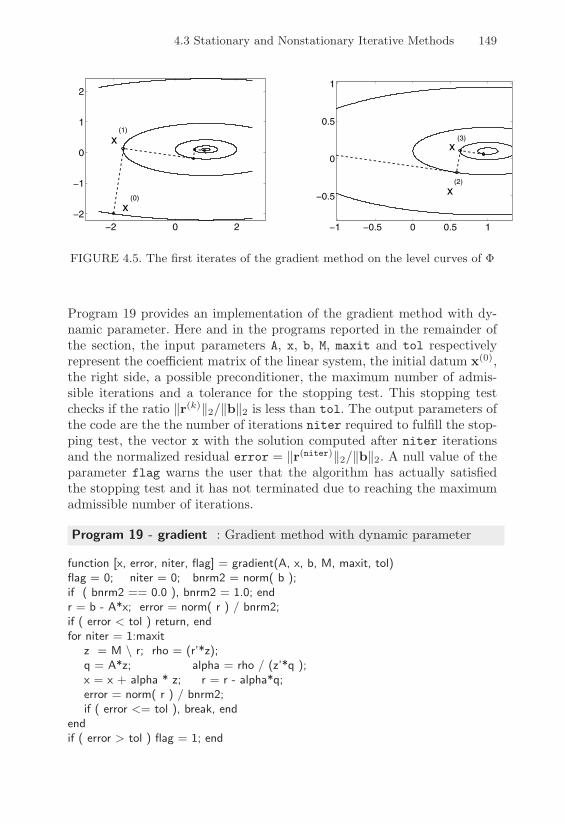
4.3 Stationary and Nonstationary Iterative Methods 149
!2 0 2!2
!1
0
1
2
x(0)
x(1)
!1 !0.5 0 0.5 1
!0.5
0
0.5
1
x(2)
x(3)
FIGURE 4.5. The first iterates of the gradient method on the level curves of %
Program 19 provides an implementation of the gradient method with dy-namic parameter. Here and in the programs reported in the remainder ofthe section, the input parameters A, x, b, M, maxit and tol respectivelyrepresent the coe"cient matrix of the linear system, the initial datum x(0),the right side, a possible preconditioner, the maximum number of admis-sible iterations and a tolerance for the stopping test. This stopping testchecks if the ratio +r(k)+2/+b+2 is less than tol. The output parameters ofthe code are the the number of iterations niter required to fulfill the stop-ping test, the vector x with the solution computed after niter iterationsand the normalized residual error = +r(niter)+2/+b+2. A null value of theparameter flag warns the user that the algorithm has actually satisfiedthe stopping test and it has not terminated due to reaching the maximumadmissible number of iterations.
Program 19 - gradient : Gradient method with dynamic parameter
function [x, error, niter, flag] = gradient(A, x, b, M, maxit, tol)flag = 0; niter = 0; bnrm2 = norm( b );if ( bnrm2 == 0.0 ), bnrm2 = 1.0; endr = b - A*x; error = norm( r ) / bnrm2;if ( error < tol ) return, endfor niter = 1:maxit
z = M \ r; rho = (r’*z);q = A*z; alpha = rho / (z’*q );x = x + alpha * z; r = r - alpha*q;error = norm( r ) / bnrm2;if ( error <= tol ), break, end
endif ( error > tol ) flag = 1; end
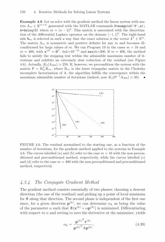
150 4. Iterative Methods for Solving Linear Systems
Example 4.6 Let us solve with the gradient method the linear system with ma-trix Am / Rm&m generated with the MATLAB commands G=numgrid(’S’,n);A=delsq(G) where m = (n % 2)2. This matrix is associated with the discretiza-tion of the di"erential Laplace operator on the domain [%1, 1]2. The right-handside bm is selected in such a way that the exact solution is the vector 1T / Rm.The matrix Am is symmetric and positive definite for any m and becomes ill-conditioned for large values of m. We run Program 19 in the cases m = 16 andm = 400, with x(0) = 0T , tol=10%10 and maxit=200. If m = 400, the methodfails to satisfy the stopping test within the admissible maximum number of it-erations and exhibits an extremely slow reduction of the residual (see Figure4.6). Actually, K2(A400) 0 258. If, however, we precondition the system with thematrix P = RT
inRin, where Rin is the lower triangular matrix in the Choleskyincomplete factorization of A, the algorithm fulfills the convergence within themaximum admissible number of iterations (indeed, now K2(P%1A400) 0 38). •
0 50 100 150 200 25010
!14
10!12
10!10
10!8
10!6
10!4
10!2
100
(a)(b)
(c)
(d)
FIGURE 4.6. The residual normalized to the starting one, as a function of thenumber of iterations, for the gradient method applied to the systems in Example4.6. The curves labelled (a) and (b) refer to the case m = 16 with the non precon-ditioned and preconditioned method, respectively, while the curves labelled (c)and (d) refer to the case m = 400 with the non preconditioned and preconditionedmethod, respectively
4.3.4 The Conjugate Gradient MethodThe gradient method consists essentially of two phases: choosing a descentdirection (the one of the residual) and picking up a point of local minimumfor ' along that direction. The second phase is independent of the first onesince, for a given direction p(k), we can determine "k as being the valueof the parameter " such that '(x(k) +"p(k)) is minimized. Di!erentiatingwith respect to " and setting to zero the derivative at the minimizer, yields
"k =p(k)T r(k)
p(k)TAp(k), (4.39)

4.3 Stationary and Nonstationary Iterative Methods 151
instead of (4.37). The question is how to determine p(k). A di!erent ap-proach than the one which led to identify p(k) with r(k) is suggested by thefollowing definition.
Definition 4.4 A direction x(k) is said to be optimal with respect to adirection p '= 0 if
'(x(k)) & '(x(k) + $p), #$ ! R. (4.40)
If x(k) is optimal with respect to any direction in a vector space V, we saythat x(k) is optimal with respect to V. !
From the definition of optimality, it turns out that p must be orthogonalto the residual r(k). Indeed, from (4.40) we conclude that ' admits a localminimum along p for $ = 0, and thus the partial derivative of ' withrespect to $ must vanish at $ = 0. Since
.'
.$(x(k) + $p) = pT (Ax(k) " b) + $pTAp,
we therefore have
.'
.$(x(k))|#=0 = 0 i! pT (r(k)) = 0,
that is, p 6 r(k). Notice that the iterate x(k+1) of the gradient methodis optimal with respect to r(k) since, due to the choice of "k, we haver(k+1) 6 r(k), but this property no longer holds for the successive iteratex(k+2) (see Exercise 12). It is then natural to ask whether there exist descentdirections that maintain the optimality of iterates. Let
x(k+1) = x(k) + q,
and assume that x(k) is optimal with respect to a direction p (thus, r(k) 6p). Let us impose that x(k+1) is still optimal with respect to p, that is,r(k+1) 6 p. We obtain
0 = pT r(k+1) = pT (r(k) "Aq) = "pTAq.
The conclusion is that, in order to preserve optimality between succes-sive iterates, the descent directions must be mutually A-orthogonal or A-conjugate, i.e.
pTAq = 0.
A method employing A-conjugate descent directions is called conjugate.The next step is how to generate automatically a sequence of conjugate

152 4. Iterative Methods for Solving Linear Systems
directions. This can be done as follows. Let p(0) = r(0) and search for thedirections of the form
p(k+1) = r(k+1) " #kp(k), k = 0, 1, . . . (4.41)
where #k ! R must be determined in such a way that
(Ap(j))Tp(k+1) = 0, j = 0, 1, . . . , k. (4.42)
Requiring that (4.42) is satisfied for j = k, we get from (4.41)
#k =(Ap(k))T r(k+1)
(Ap(k))Tp(k) , k = 0, 1, . . .
We must now verify that (4.42) holds also for j = 0, 1, . . . , k"1. To do this,let us proceed by induction on k. Due to the choice of #0, relation (4.42)holds for k = 0; let us thus assume that the directions p(0), . . . ,p(k"1) aremutually A-orthogonal and, without losing generality, that
(p(j))T r(k) = 0, j = 0, 1, . . . , k " 1, k ) 1. (4.43)
Then, from (4.41) it follows that
(Ap(j))Tp(k+1) = (Ap(j))T r(k+1), j = 0, 1, . . . , k " 1.
Moreover, due to (4.43) and by the assumption of of A-orthogonality weget
(p(j))T r(k+1) = (p(j))T r(k) " "k(p(j))TAp(k) = 0, j = 0, . . . , k " 1(4.44)
i.e., we conclude that r(k+1) is orthogonal to every vector of the space Vk =span(p(0), . . . ,p(k"1)). Since p(0) = r(0), from (4.41) it follows that Vk isalso equal to span(r(0), . . . , r(k"1)). Then, (4.41) implies that Ap(j) ! Vj+1and thus, due to (4.44)
(Ap(j))T r(k+1) = 0, j = 0, 1, . . . , k " 1.
As a consequence, (4.42) holds for j = 0, . . . , k.
The conjugate gradient method (CG) is the method obtained by choosingthe descent directions p(k) given by (4.41) and the acceleration parameter"k as in (4.39). As a consequence, setting r(0) = b"Ax(0) and p(0) = r(0),the k-th iteration of the conjugate gradient method takes the following

4.3 Stationary and Nonstationary Iterative Methods 153
0 0.2 0.4 0.6 0.8 1 1.2 1.4 1.6 1.8
!0.2
0
0.2
0.4
0.6
0.8
1
1.2
1.4
CG
G
FIGURE 4.7. Descent directions for the conjugate gradient method (denoted byCG, dashed line) and the gradient method (denoted by G, solid line). Notice thatthe CG method reaches the solution after two iterations
form
"k =p(k)T r(k)
p(k)TAp(k)
x(k+1) = x(k) + "kp(k)
r(k+1) = r(k) " "kAp(k)
#k =(Ap(k))T r(k+1)
(Ap(k))Tp(k)
p(k+1) = r(k+1) " #kp(k).
It can also be shown (see Exercise 13) that the two parameters "k and #kmay be alternatively expressed as
"k =+r(k)+22
p(k)TAp(k), #k =
+r(k+1)+22+r(k)+22
. (4.45)
We finally notice that, eliminating the descent directions from r(k+1) =r(k) " "kAp(k), the following recursive three-terms relation is obtained forthe residuals (see Exercise 14)
Ar(k) = " 1"k
r(k+1) +4
1"k" #k"1
"k"1
5r(k) +
#k"k"1
r(k"1). (4.46)
As for the convergence of the CG method, we have the following results.
Theorem 4.11 Let A be a symmetric and positive definite matrix. Anymethod which employs conjugate directions to solve (3.2) terminates afterat most n steps, yielding the exact solution.

154 4. Iterative Methods for Solving Linear Systems
Proof. The directions p(0),p(1), . . . ,p(n%1) form an A-orthogonal basis in Rn.Moreover, since x(k) is optimal with respect to all the directions p(j), j =0, . . . , k%1, it follows that r(k) is orthogonal to the space Sk%1 = span(p(0),p(1),
. . . ,p(k%1)). As a consequence, r(n) 3 Sn%1 = Rn and thus r(n) = 0 whichimplies x(n) = x. !
Theorem 4.12 Let A be a symmetric and positive definite matrix andlet $1, $n be its maximum and minimum eigenvalues, respectively. Theconjugate gradient method for solving (3.2) converges after at most n steps.Moreover, the error e(k) at the k-th iteration (with k < n) is orthogonal top(j), for j = 0, . . . , k " 1 and
+e(k)+A &2ck
1 + c2k+e(0)+A, with c =
3K2(A)" 1
3K2(A) + 1
. (4.47)
Proof. The convergence of the CG method in n steps is a consequence of The-orem 4.11.
Let us prove the error estimate, assuming for simplicity that x(0) = 0. Noticefirst that, for fixed k
x(k+1) =k(
j=0
,jAjb,
for suitable ,j / R. Moreover, by construction, x(k+1) is the vector which min-imizes the A-norm of the error at step k + 1, among all vectors of the formz =
!kj=0 !jAjb = pk(A)b, where pk(/) =
!kj=0 !j/
j is a polynomial of degreek and pk(A) denotes the corresponding matrix polynomial. As a consequence
&e(k+1)&2A " (x% z)TA(x% z) = xT qk+1(A)Aqk+1(A)x, (4.48)
where qk+1(/) = 1 % pk(/)/ / P0,1k+1, being P
0,1k+1 = {q / Pk+1 : q(0) = 1} and
qk+1(A) the associated matrix polynomial. From (4.48) we get
&e(k+1)&2A = minqk+1'P
0,1k+1
xT qk+1(A)Aqk+1(A)x. (4.49)
Since A is symmetric positive definite, there exists an orthogonal matrix Qsuch that A = Q&QT with & = diag(#1, . . . ,#n). Noticing that qk+1(A) =Qqk+1(&)QT , we get from (4.49)
&e(k+1)&2A = minqk+1'P
0,1k+1
xTQqk+1(&)QTQ&QTQqk+1(&)QTx
= minqk+1'P
0,1k+1
xTQqk+1(&)&qk+1(&)QTx
= minqk+1'P
0,1k+1
yTdiag(qk+1(#i)#iqk+1(#i))y
= minqk+1'P
0,1k+1
n(
i=1
y2i #i(qk+1(#i))2

4.3 Stationary and Nonstationary Iterative Methods 155
having set y = Qx. Thus, we can conclude that
&e(k+1)&2A "N
minqk+1'P
0,1k+1
max%i'&(A)
(qk+1(#i))2O
n(
i=1
y2i #i.
Recalling thatn(
i=1
y2i #i = &e(0)&2A, we have
&e(k+1)&A&e(0)&A
" minqk+1'P
0,1k+1
max%i'&(A)
|qk+1(#i)|.
Let us now recall the following property
Property 4.6 The problem of minimizing max%n*z*%1
|q(z)| over the space
P0,1k+1([#n,#1]) admits a unique solution, given by the polynomial
pk+1(/) = Tk+1
4#1 + #n % 2/
#1 % #n
5/Ck+1, / / [#n,#1],
where Ck+1 = Tk+1(%1+%n%1%%n
) and Tk+1 is the Chebyshev polynomial of degree k+1(see Section 10.10). The value of the minimum is 1/Ck+1.
Using this property we get
&e(k+1)&A&e(0)&A
" 1
Tk+1
4#1 + #n
#1 % #n
5
from which the thesis follows since in the case of a symmetric positive definitematrix
1Ck+1
=2ck+1
1 + c2(k+1) .
!
The generic k-th iteration of the conjugate gradient method is well definedonly if the descent direction p(k) is non null. Besides, if p(k) = 0, then theiterate x(k) must necessarily coincide with the solution x of the system.Moreover, irrespectively of the choice of the parameters #k, one can show(see [Axe94], p. 463) that the sequence x(k) generated by the CG methodis such that either x(k) '= x, p(k) '= 0, "k '= 0 for any k, or there must existan integer m such that x(m) = x, where x(k) '= x, p(k) '= 0 and "k '= 0 fork = 0, 1, . . . ,m" 1.
The particular choice made for #k in (4.45) ensures that m & n. In ab-sence of rounding errors, the CG method can thus be regarded as being adirect method, since it terminates after a finite number of steps. However,for matrices of large size, it is usually employed as an iterative scheme,

156 4. Iterative Methods for Solving Linear Systems
where the iterations are stopped when the error gets below a fixed toler-ance. In this respect, the dependence of the error reduction factor on thecondition number of the matrix is more favorable than for the gradientmethod. We also notice that estimate (4.47) is often overly pessimistic anddoes not account for the fact that in this method, unlike what happens forthe gradient method, the convergence is influenced by the whole spectrumof A, and not only by its extremal eigenvalues.
Remark 4.3 (E!ect of rounding errors) The termination property ofthe CG method is rigorously valid only in exact arithmetic. The cumulatingrounding errors prevent the descent directions from being A-conjugate andcan even generate null denominators in the computation of coe"cients "k
and #k. This latter phenomenon, known as breakdown, can be avoided byintroducing suitable stabilization procedures; in such an event, we speakabout stabilized gradient methods.
Despite the use of these strategies, it may happen that the CG methodfails to converge (in finite arithmetic) after n iterations. In such a case,the only reasonable possibility is to restart the iterative process, takingas residual the last computed one. By so doing, the cyclic CG method orCG method with restart is obtained, for which, however, the convergenceproperties of the original CG method are no longer valid. !
4.3.5 The Preconditioned Conjugate Gradient MethodIf P is a symmetric and positive definite preconditioning matrix, the pre-conditioned conjugate gradient method (PCG) consists of applying the CGmethod to the preconditioned system
P"1/2AP"1/2y = P"1/2b, with y = P1/2x.
In practice, the method is implemented without explicitly requiring thecomputation of P1/2 or P"1/2. After some algebra, the following scheme isobtained:given x(0) and setting r(0) = b " Ax(0), z(0) = P"1r(0) e p(0) = z(0), thek-th iteration reads

4.3 Stationary and Nonstationary Iterative Methods 157
"k =p(k)T r(k)
p(k)TAp(k)
x(k+1) = x(k) + "kp(k)
r(k+1) = r(k) " "kAp(k)
Pz(k+1) = r(k+1)
#k =(Ap(k))T z(k+1)
(Ap(k))Tp(k)
p(k+1) = z(k+1) " #kp(k).
The computational cost is increased with respect to the CG method, asone needs to solve at each step the linear system Pz(k+1) = r(k+1). For thissystem the symmetric preconditioners examined in Section 4.3.2 can beused. The error estimate is the same as for the nonpreconditioned method,provided to replace the matrix A by P"1A.
In Program 20 an implementation of the PCG method is reported. Fora description of the input/output parameters, see Program 19.
Program 20 - conjgrad : Preconditioned conjugate gradient method
function [x, error, niter, flag] = conjgrad(A, x, b, P, maxit, tol)flag = 0; niter = 0; bnrm2 = norm( b );if ( bnrm2 == 0.0 ), bnrm2 = 1.0; endr = b - A*x; error = norm( r ) / bnrm2;if ( error < tol ) return, endfor niter = 1:maxit
z = P \ r; rho = (r’*z);if niter > 1
beta = rho / rho1; p = z + beta*p;else
p = z;endq = A*p; alpha = rho / (p’*q );x = x + alpha * p; r = r - alpha*q;error = norm( r ) / bnrm2;if ( error <= tol ), break, endrho1 = rho;
endif ( error > tol ) flag = 1; end

158 4. Iterative Methods for Solving Linear Systems
Example 4.7 Let us consider again the linear system of Example 4.6. The CGmethod has been run with the same input data as in the previous example. Itconverges in 3 iterations for m = 16 and in 45 iterations for m = 400. Using thesame preconditioner as in Example 4.6, the number of iterations decreases from45 to 26, in the case m = 400. •
0 5 10 15 20 25 30 35 40 4510
!14
10!12
10!10
10!8
10!6
10!4
10!2
100
FIGURE 4.8. Behavior of the residual, normalized to the right-hand side, as afunction of the number of iterations for the conjugate gradient method appliedto the systems of Example 4.6 in the case m = 400. The curve in dashed linerefers to the non preconditioned method, while the curve in solid line refers tothe preconditioned one
4.3.6 The Alternating-Direction MethodAssume that A = A1+A2, with A1 and A2 symmetric and positive definite.The alternating direction method (ADI), as introduced by Peaceman andRachford [PJ55], is an iterative scheme for (3.2) which consists of solvingthe following systems #k ) 0
(I + "1A1)x(k+1/2) = (I" "1A2)x(k) + "1b,
(I + "2A2)x(k+1) = (I" "2A1)x(k+1/2) + "2b(4.50)
where "1 and "2 are two real parameters. The ADI method can be cast inthe form (4.2) setting
B = (I + "2A2)"1(I" "2A1)(I + "1A1)"1(I" "1A2),
f =P"1(I" "2A1)(I + "1A1)"1 + "2I
Qb.
Both B and f depend on "1 and "2. The following estimate holds
)(B) & maxi=1,... ,n
>>>>>1" "2$
(1)i
1 + "1$(1)i
>>>>> maxi=1,... ,n
>>>>>1" "1$
(2)i
1 + "2$(2)i
>>>>> ,

4.4 Methods Based on Krylov Subspace Iterations 159
where $(i)1 and $(i)
2 , for i = 1, . . . , n, are the eigenvalues of A1 and A2,respectively. The method converges if )(B) < 1, which is always verified if"1 = "2 = " > 0. Moreover (see [Axe94]) if ' & $(j)
i & % #i = 1, . . . , n,#j = 1, 2, for suitable ' and % then the ADI method converges with thechoice "1 = "2 = 1/
/%', provided that '/% tends to 0 as the size of A
grows. In such an event the corresponding spectral radius satisfies
)(B) &6
1"3'/%
1 +3'/%
72
.
4.4 Methods Based on Krylov Subspace Iterations
In this section we introduce iterative methods based on Krylov subspaceiterations. For the proofs and further analysis, we refer to [Saa96], [Axe94]and [Hac94].
Consider the Richardson method (4.24) with P=I; the residual at thek-th step can be related to the initial residual as
r(k) =k"11
j=0
(I" "jA)r(0) (4.51)
so that r(k) = pk(A)r(0), where pk(A) is a polynomial in A of degree k. Ifwe introduce the space
Km(A;v) = span/v,Av, . . . ,Am"1v
0, (4.52)
it immediately appears from (4.51) that r(k) ! Kk+1(A; r(0)). The spacedefined in (4.52) is called the Krylov subspace of order m. It is a subspaceof the set spanned by all the vectors u ! Rn that can be written as u =pm"1(A)v, where pm"1 is a polynomial in A of degree & m" 1.
In an analogous manner as for (4.51), it is seen that the iterate x(k) ofthe Richardson method is given by
x(k) = x(0) +k"1(
j=0
"jr(j)
so that x(k) belongs to the following space
Wk =Rv = x(0) + y, y ! Kk(A; r(0))
S. (4.53)
Notice also that!k"1
j=0 "jr(j) is a polynomial in A of degree less than k"1.In the non preconditioned Richardson method we are thus looking for an

160 4. Iterative Methods for Solving Linear Systems
approximate solution to x in the space Wk. More generally, we can thinkof devising methods that search for approximate solutions of the form
x(k) = x(0) + qk"1(A)r(0), (4.54)
where qk"1 is a polynomial selected in such a way that x(k) be, in a sensethat must be made precise, the best approximation of x in Wk. A methodthat looks for a solution of the form (4.54) with Wk defined as in (4.53) iscalled a Krylov method.
A first question concerning Krylov subspace iterations is whether thedimension of Km(A;v) increases as the order m grows. A partial answer isprovided by the following result.
Property 4.7 Let A ! Rn!n and v ! Rn. The Krylov subspace Km(A;v)has dimension equal to m i! the degree of v with respect to A, denoted bydegA(v), is not less than m, where the degree of v is defined as the minimumdegree of a monic non null polynomial p in A, for which p(A)v = 0.
The dimension of Km(A;v) is thus equal to the minimum between m andthe degree of v with respect to A and, as a consequence, the dimensionof the Krylov subspaces is certainly a nondecreasing function of m. Noticethat the degree of v cannot be greater than n due to the Cayley-HamiltonTheorem (see Section 1.7).
Example 4.8 Consider the matrix A = tridiag4(%1, 2,%1). The vector v =(1, 1, 1, 1)T has degree 2 with respect to A since p2(A)v = 0 with p2(A) = I4 %3A+A2, while there is no monic polynomial p1 of degree 1 for which p1(A)v = 0.As a consequence, all Krylov subspaces from K2(A;v) on, have dimension equalto 2. The vector w = (1, 1,%1, 1)T has, instead, degree 4 with respect to A. •
For a fixed m, it is possible to compute an orthonormal basis for Km(A;v)using the so-called Arnoldi algorithm.
Setting v1 = v/+v+2, this method generates an orthonormal basis {vi}for Km(A;v1) using the Gram-Schmidt procedure (see Section 3.4.3). Fork = 1, . . . ,m, the Arnoldi algorithm computes
hik = vTi Avk, i = 1, 2, . . . , k,
wk = Avk "k(
i=1
hikvi, hk+1,k = +wk+2.(4.55)
If wk = 0 the process terminates and in such a case we say that a breakdownof the algorithm has occurred; otherwise, we set vk+1 = wk/+wk+2 and thealgorithm restarts, incrementing k by 1.

4.4 Methods Based on Krylov Subspace Iterations 161
It can be shown that if the method terminates at the step m then thevectors v1, . . . ,vm form a basis for Km(A;v). In such a case, if we denoteby Vm ! Rn!m the matrix whose columns are the vectors vi, we have
VTmAVm = Hm, VT
m+1AVm = :Hm, (4.56)
where :Hm ! R(m+1)!m is the upper Hessenberg matrix whose entries hij
are given by (4.55) and Hm ! Rm!m is the restriction of :Hm to the first mrows and m columns.
The algorithm terminates at an intermediate step k < m i! degA(v1) =k. As for the stability of the procedure, all the considerations valid for theGram-Schmidt method hold. For more e"cient and stable computationalvariants of (4.55), we refer to [Saa96].
The functions arnoldi alg and GSarnoldi, invoked by Program 21, pro-vide an implementation of the Arnoldi algorithm. In output, the columnsof V contain the vectors of the generated basis, while the matrix H storesthe coe"cients hik computed by the algorithm. If m steps are carried out,V = Vm and H(1 : m, 1 : m) = Hm.
Program 21 - arnoldi alg : The Arnoldi algorithm
function [V,H]=arnoldi alg(A,v,m)v=v/norm(v,2); V=[v1]; H=[]; k=0;while k <= m-1
[k,V,H] = GSarnoldi(A,m,k,V,H);end
function [k,V,H]=GSarnoldi(A,m,k,V,H)k=k+1; H=[H,V(:,1:k)’*A*V(:,k)];s=0; for i=1:k, s=s+H(i,k)*V(:,i); endw=A*V(:,k)-s; H(k+1,k)=norm(w,2);if ( H(k+1,k) <= eps ) & ( k < m )
V=[V,w/H(k+1,k)];else
k=m+1;end
Having introduced an algorithm for generating the basis for a Krylov sub-space of any order, we can now solve the linear system (3.2) by a Krylovmethod. As already noticed, for all of these methods the iterate x(k) isalways of the form (4.54) and, for a given r(0), the vector x(k) is selected asbeing the unique element in Wk which satisfies a criterion of minimal dis-tance from x. Thus, the feature distinguishing two di!erent Krylov methodsis the criterion for selecting x(k).
The most natural idea consists of searching for x(k) ! Wk as the vectorwhich minimizes the Euclidean norm of the error. This approach, how-

162 4. Iterative Methods for Solving Linear Systems
ever, does not work in practice since x(k) would depend on the (unknown)solution x.
Two alternative strategies can be pursued:
1. compute x(k) ! Wk enforcing that the residual r(k) is orthogonal toany vector in Kk(A; r(0)), i.e., we look for x(k) !Wk such that
vT (b"Ax(k)) = 0 #v ! Kk(A; r(0)); (4.57)
2. compute x(k) ! Wk minimizing the Euclidean norm of the residual+r(k)+2, i.e.
+b"Ax(k)+2 = minv#Wk
+b"Av+2. (4.58)
Satisfying (4.57) leads to the Arnoldi method for linear systems (morecommonly known as FOM, full orthogonalization method), while satisfying(4.58) yields the GMRES (generalized minimum residual) method.
In the two forthcoming sections we shall assume that k steps of theArnoldi algorithm have been carried out, in such a way that an orthonormalbasis for Kk(A; r(0)) has been generated and stored into the column vectorsof the matrix Vk with v1 = r(0)/+r(0)+2. In such a case the new iterate x(k)
can always be written as
x(k) = x(0) + Vkz(k), (4.59)
where z(k) must be selected according to a fixed criterion.
4.4.1 The Arnoldi Method for Linear SystemsLet us enforce that r(k) be orthogonal to Kk(A; r(0)) by requiring that(4.57) holds for all the basis vectors vi, i.e.
VTk r(k) = 0. (4.60)
Since r(k) = b"Ax(k) with x(k) of the form (4.59), relation (4.60) becomes
VTk (b"Ax(0))"VT
k AVkz(k) = VTk r(0) "VT
k AVkz(k) = 0. (4.61)
Due to the orthonormality of the basis and the choice of v1, VTk r(0) =
+r(0)+2e1, e1 being the first unit vector of Rm. Recalling (4.56), from (4.61)it turns out that z(k) is the solution to the linear system
Hkz(k) = +r(0)+2e1. (4.62)
Once z(k) is known, we can compute x(k) from (4.59). Since Hk is an upperHessenberg matrix, the linear system in (4.62) can be easily solved, forinstance, resorting to the LU factorization of Hk.

4.4 Methods Based on Krylov Subspace Iterations 163
We notice that the method, if working in exact arithmetic, cannot executemore than n steps and that it terminates after m < n steps only if abreakdown in the Arnoldi algorithm occurs. As for the convergence of themethod, the following result holds.
Theorem 4.13 In exact arithmetic the Arnoldi method yields the solutionof (3.2) after at most n iterations.
Proof. If the method terminates at the n-th iteration, then it must necessarilybe x(n) = x since Kn(A; r(0)) = Rn. Conversely, if a breakdown occurs after miterations, for a suitable m < n, then x(m) = x. Indeed, inverting the first relationin (4.56), we get
x(m) = x(0) + Vmz(m) = x(0) + VmH%1m VT
mr(0) = A%1b.
!
In its naive form, FOM does not require an explicit computation of thesolution or the residual, unless a breakdown occurs. Therefore, monitoringits convergence (by computing, for instance, the residual at each step) mightbe computationally expensive. The residual, however, is available withoutexplicitly requiring to compute the solution since at the k-th step we have
+b"Ax(k)+2 = hk+1,k|eTk zk|
and, as a consequence, one can decide to stop the method if
hk+1,k|eTk zk|/+r(0)+2 & + (4.63)
+ > 0 being a fixed tolerance.
The most relevant consequence of Theorem 4.13 is that FOM can beregarded as a direct method, since it yields the exact solution after a finitenumber of steps. However, this fails to hold when working in floating pointarithmetic due to the cumulating rounding errors. Moreover, if we alsoaccount for the high computational e!ort, which, for a number of m stepsand a sparse matrix of order n with nz nonzero entries, is of the order of2(nz + mn) flops, and the large memory occupation needed to store thematrix Vm, we conclude that the Arnoldi method cannot be used in thepractice, except for small values of m.
Several remedies to this drawback are available, one of which consistingof preconditioning the system (using, for instance, one of the precondition-ers proposed in Section 4.3.2). Alternatively, we can also introduce somemodified versions of the Arnoldi method following two approaches:
1. no more than m consecutive steps of FOM are taken, m being a smallfixed number (usually, m 1 10). If the method fails to converge, we set
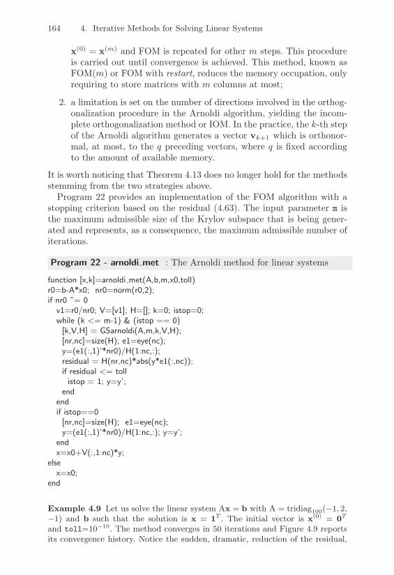
164 4. Iterative Methods for Solving Linear Systems
x(0) = x(m) and FOM is repeated for other m steps. This procedureis carried out until convergence is achieved. This method, known asFOM(m) or FOM with restart, reduces the memory occupation, onlyrequiring to store matrices with m columns at most;
2. a limitation is set on the number of directions involved in the orthog-onalization procedure in the Arnoldi algorithm, yielding the incom-plete orthogonalization method or IOM. In the practice, the k-th stepof the Arnoldi algorithm generates a vector vk+1 which is orthonor-mal, at most, to the q preceding vectors, where q is fixed accordingto the amount of available memory.
It is worth noticing that Theorem 4.13 does no longer hold for the methodsstemming from the two strategies above.
Program 22 provides an implementation of the FOM algorithm with astopping criterion based on the residual (4.63). The input parameter m isthe maximum admissible size of the Krylov subspace that is being gener-ated and represents, as a consequence, the maximum admissible number ofiterations.
Program 22 - arnoldi met : The Arnoldi method for linear systems
function [x,k]=arnoldi met(A,b,m,x0,toll)r0=b-A*x0; nr0=norm(r0,2);if nr0 ˜= 0
v1=r0/nr0; V=[v1]; H=[]; k=0; istop=0;while (k <= m-1) & (istop == 0)[k,V,H] = GSarnoldi(A,m,k,V,H);[nr,nc]=size(H); e1=eye(nc);y=(e1(:,1)’*nr0)/H(1:nc,:);residual = H(nr,nc)*abs(y*e1(:,nc));if residual <= tollistop = 1; y=y’;
endendif istop==0[nr,nc]=size(H); e1=eye(nc);y=(e1(:,1)’*nr0)/H(1:nc,:); y=y’;
endx=x0+V(:,1:nc)*y;
elsex=x0;
end
Example 4.9 Let us solve the linear system Ax = b with A = tridiag100(%1, 2,%1) and b such that the solution is x = 1T . The initial vector is x(0) = 0T
and toll=10%10. The method converges in 50 iterations and Figure 4.9 reportsits convergence history. Notice the sudden, dramatic, reduction of the residual,

4.4 Methods Based on Krylov Subspace Iterations 165
which is a typical warning that the last generated subspace Wk is su!ciently richto contain the exact solution of the system. •
0 10 20 30 40 50 6010
!16
10!14
10!12
10!10
10!8
10!6
10!4
10!2
100
102
FIGURE 4.9. The behavior of the residual as a function of the number of itera-tions for the Arnoldi method applied to the linear system in Example 4.9
4.4.2 The GMRES MethodThis method is characterized by selecting x(k) in such a way to minimizethe Euclidean norm of the residual at each k-th step. Recalling (4.59) wehave
r(k) = r(0) "AVkz(k), (4.64)
but, since r(0) = v1+r(0)+2 and (4.56) holds, relation (4.64) becomes
r(k) = Vk+1(+r(0)+2e1 " :Hkz(k)), (4.65)
where e1 is the first unit vector of Rk+1. Therefore, in the GMRES methodthe solution at step k can be computed through (4.59) as
z(k) chosen in such a way to minimize + +r(0)+2e1 " :Hkz(k)+2 (4.66)
(the matrix Vk+1 appearing in (4.65) does not change the value of + · +2since it is orthogonal). Having to solve at each step a least-squares problemof size k, the GMRES method will be the more e!ective the smaller isthe number of iterations. Exactly as for the Arnoldi method, the GMRESmethod terminates at most after n iterations, yielding the exact solution.Premature stops are due to a breakdown in the orthonormalization Arnoldialgorithm. More precisely, we have the following result.
Property 4.8 A breakdown occurs for the GMRES method at a step m(with m < n) i! the computed solution x(m) coincides with the exact solu-tion to the system.

166 4. Iterative Methods for Solving Linear Systems
A basic implementation of the GMRES method is provided in Program 23.This latter requires in input the maximum admissible size m for the Krylovsubspace and the tolerance toll on the Euclidean norm of the residualnormalized to the initial residual. This implementation of the method com-putes the solution x(k) at each step in order to evaluate the residual, witha consequent increase of the computational e!ort.
Program 23 - GMRES : The GMRES method for linear systems
function [x,k]=gmres(A,b,m,toll,x0)r0=b-A*x0; nr0=norm(r0,2);if nr0 ˜= 0v1=r0/nr0; V=[v1]; H=[]; k=0; residual=1;while k <= m-1 & residual > toll,[k,V,H] = GSarnoldi(A,m,k,V,H);[nr,nc]=size(H); y=(H’*H) \ (H’*nr0*[1;zeros(nr-1,1)]);x=x0+V(:,1:nc)*y; residual = norm(b-A*x,2)/nr0;
endelsex=x0;
end
To improve the e"ciency of the GMRES algorithm it is necessary to devisea stopping criterion which does not require the explicit evaluation of theresidual at each step. This is possible, provided that the linear system withupper Hessenberg matrix :Hk is appropriately solved.
In practice, :Hk is transformed into an upper triangular matrix Rk !R(k+1)!k with rk+1,k = 0 such that QT
k Rk = :Hk, where Qk is a matrixobtained as the product of k Givens rotations (see Section 5.6.3). Then,since Qk is orthogonal, it can be seen that minimizing ++r(0)+2e1":Hkz(k)+2is equivalent to minimize +fk " Rkz(k)+2, with fk = Qk+r(0)+2e1. It canalso be shown that the k + 1-th component of fk is, in absolute value, theEuclidean norm of the residual at the k-th step.
As FOM, the GMRES method entails a high computational e!ort anda large amount of memory, unless convergence occurs after few iterations.For this reason, two variants of the algorithm are available, one namedGMRES(m) and based on the restart after m steps, the other named Quasi-GMRES or QGMRES and based on stopping the Arnoldi orthogonalizationprocess. It is worth noting that these two methods do not enjoy Property4.8.
Remark 4.4 (Projection methods) Denoting by Yk and Lk two genericm-dimensional subspaces of Rn, we call projection method a process whichgenerates an approximate solution x(k) at step k, enforcing that x(k) ! Yk
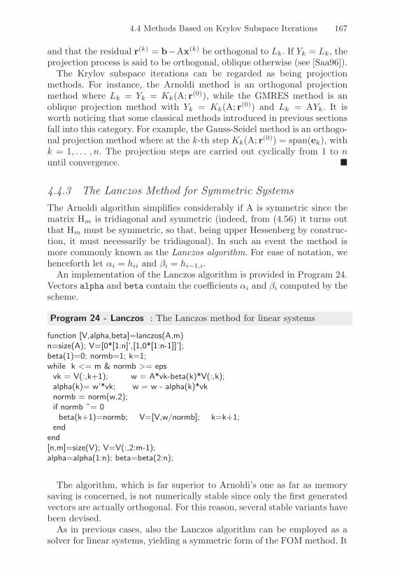
4.4 Methods Based on Krylov Subspace Iterations 167
and that the residual r(k) = b"Ax(k) be orthogonal to Lk. If Yk = Lk, theprojection process is said to be orthogonal, oblique otherwise (see [Saa96]).
The Krylov subspace iterations can be regarded as being projectionmethods. For instance, the Arnoldi method is an orthogonal projectionmethod where Lk = Yk = Kk(A; r(0)), while the GMRES method is anoblique projection method with Yk = Kk(A; r(0)) and Lk = AYk. It isworth noticing that some classical methods introduced in previous sectionsfall into this category. For example, the Gauss-Seidel method is an orthogo-nal projection method where at the k-th step Kk(A; r(0)) = span(ek), withk = 1, . . . , n. The projection steps are carried out cyclically from 1 to nuntil convergence. !
4.4.3 The Lanczos Method for Symmetric SystemsThe Arnoldi algorithm simplifies considerably if A is symmetric since thematrix Hm is tridiagonal and symmetric (indeed, from (4.56) it turns outthat Hm must be symmetric, so that, being upper Hessenberg by construc-tion, it must necessarily be tridiagonal). In such an event the method ismore commonly known as the Lanczos algorithm. For ease of notation, wehenceforth let "i = hii and #i = hi"1,i.
An implementation of the Lanczos algorithm is provided in Program 24.Vectors alpha and beta contain the coe"cients "i and #i computed by thescheme.
Program 24 - Lanczos : The Lanczos method for linear systems
function [V,alpha,beta]=lanczos(A,m)n=size(A); V=[0*[1:n]’,[1,0*[1:n-1]]’];beta(1)=0; normb=1; k=1;while k <= m & normb >= epsvk = V(:,k+1); w = A*vk-beta(k)*V(:,k);alpha(k)= w’*vk; w = w - alpha(k)*vknormb = norm(w,2);if normb ˜= 0beta(k+1)=normb; V=[V,w/normb]; k=k+1;
endend[n,m]=size(V); V=V(:,2:m-1);alpha=alpha(1:n); beta=beta(2:n);
The algorithm, which is far superior to Arnoldi’s one as far as memorysaving is concerned, is not numerically stable since only the first generatedvectors are actually orthogonal. For this reason, several stable variants havebeen devised.
As in previous cases, also the Lanczos algorithm can be employed as asolver for linear systems, yielding a symmetric form of the FOM method. It
168 4. Iterative Methods for Solving Linear Systems
can be shown that r(k) = 'kvk+1, for a suitable 'k (analogously to (4.63))so that the residuals are all mutually orthogonal.
Remark 4.5 (The conjugate gradient method) If A is symmetric andpositive definite, starting from the Lanczos method for linear systems it ispossible to derive the conjugate gradient method already introduced in Sec-tion 4.3.4 (see [Saa96]). The conjugate gradient method is a variant of theLanczos method where the orthonormalization process remains incomplete.
As a matter of fact, the A-conjugate directions of the CG method canbe characterized as follows. If we carry out at the generic k-th step theLU factorization Hk = LkUk, with Lk (Uk) lower (upper) bidiagonal, theiterate x(k) of the Lanczos method for systems reads
x(k) = x(0) + PkL"1k +r(0)+2e1,
with Pk = VkU"1k . The column vectors of Pk are mutually A-conjugate.
Indeed, PTk APk is symmetric and bidiagonal since
PTk APk = U"T
k HkU"1k = U"T
k Lk,
so that it must necessarily be diagonal. As a result, pTj Api = 0 if i '= j,
having denoted by pi the i-th column vector of matrix Pk. !
As happens for the FOM method, also the GMRES method simplifiesif A is symmetric. The resulting scheme is called conjugate residuals orCR method since it enjoys the property that the residuals are mutuallyA-conjugate. Variants of this method are the generalized conjugate resid-uals method (GCR) and the method commonly known as ORTHOMIN(obtained by truncation of the orthonormalization process as done for theIOM method).
4.5 The Lanczos Method for Unsymmetric Systems
The Lanczos orthogonalization process can be extended to deal with un-symmetric matrices through a bi-orthogonalization procedure as follows.Two bases, {vi}mi=1 and {zi}mi=1, are generated for the subspaces Km(A;v1)and Km(AT ; z1), respectively, with zT1 v1 = 1, such that
zTi vj = %ij , i, j = 1, . . . ,m. (4.67)
Two sets of vectors satisfying (4.67) are said to be bi-orthogonal and canbe obtained through the following algorithm: setting #1 = '1 = 0 and z0 =v0 = 0T , at the generic k-th step, with k = 1, . . . ,m, we set "k = zTk Avk,then we compute
vk+1 = Avk " "kvk " #kvk"1, zk+1 = AT zk " "kzk " 'kzk"1.

4.5 The Lanczos Method for Unsymmetric Systems 169
If 'k+1 =2|zTk+1vk+1| = 0 the algorithm is stopped, otherwise we set
#k+1 = zTk+1vk+1/'k+1 and generate two new vectors in the basis as
vk+1 = vk+1/'k+1, zk+1 = zk+1/#k+1.
If the process terminates after m steps, denoting by Vm and Zm the ma-trices whose columns are the vectors of the basis that has been generated,we have
ZTmAVm = Tm,
Tm being the following tridiagonal matrix
Tm =
"
#####$
"1 #2 0'2 "2
. . .. . . . . . #m
0 'm "m
%
&&&&&'.
As in the symmetric case, the bi-orthogonalization Lanczos algorithm canbe utilized to solve the linear system (3.2). For this purpose, for m fixed,once the bases {vi}mi=1 and {zi}mi=1 have been constructed, it su"ces to set
x(m) = x(0) + Vmy(m),
where y(m) is the solution to the linear system Tmy(m) = +r(0)+2e1. Itis also possible to introduce a stopping criterion based on the residual,without computing it explicitly, since
+r(m)+2 = |'m+1eTmym| +vm+1+2.
An implementation of the Lanczos method for unsymmetric systems isgiven in Program 25. If a breakdown of the algorithm occurs, i.e., if 'k+1 =0, the method stops returning in output a negative value of the variableniter which denotes the number of iterations necessary to reduce the initialresidual by a factor toll.

170 4. Iterative Methods for Solving Linear Systems
Program 25 - Lanczosnosym : The Lanczos method for unsymmetricsystemsfunction [xk,nres,niter]=lanczosnosym(A,b,x0,m,toll)r0=b-A*x0; nres0=norm(r0,2);if nres0 ˜= 0V=r0/nres0; Z=V; gamma(1)=0; beta(1)=0; k=1; nres=1;while k <= m & nres > toll
vk=V(:,k); zk=Z(:,k);if k==1, vk1=0*vk; zk1=0*zk;else, vk1=V(:,k-1); zk1=Z(:,k-1); endalpha(k)=zk’*A*vk;tildev=A*vk-alpha(k)*vk-beta(k)*vk1;tildez=A’*zk-alpha(k)*zk-gamma(k)*zk1;gamma(k+1)=sqrt(abs(tildez’*tildev));if gamma(k+1) == 0, k=m+2;elsebeta(k+1)=tildez’*tildev/gamma(k+1);Z=[Z,tildez/beta(k+1)];V=[V,tildev/gamma(k+1)];
endif k˜=m+2if k==1Tk = alpha;
elseTk=diag(alpha)+diag(beta(2:k),1)+diag(gamma(2:k),-1);
endyk=Tk \ (nres0*[1,0*[1:k-1]]’);xk=x0+V(:,1:k)*yk;nres=abs(gamma(k+1)*[0*[1:k-1],1]*yk)*norm(V(:,k+1),2)/nres0;k=k+1;
endendelsex=x0;
endif k==m+2, niter=-k; else, niter=k-1; end
Example 4.10 Let us solve the linear system with matrix A = tridiag100(%0.5, 2,%1) and right-side b selected in such a way that the exact solution is x = 1T .Using Program 25 with toll= 10%13 and a randomly generated x0, the algorithmconverges in 59 iterations. Figure 4.10 shows the convergence history reportingthe graph of &r(k)&2/&r(0)&2 as a function of the number of iterations. •
We conclude recalling that some variants of the unsymmetric Lanczosmethod have been devised, that are characterized by a reduced compu-tational cost. We refer the interested reader to the bibliography below for a

4.6 Stopping Criteria 171
0 10 20 30 40 50 6010
!14
10!12
10!10
10!8
10!6
10!4
10!2
100
FIGURE 4.10. Graph of the residual normalized to the initial residual as a func-tion of the number of iterations for the Lanczos method applied to the system inExample 4.10
complete description of the algorithms and to the programs included in theMATLAB version of the public domain library templates for their e"cientimplementation [BBC+94].
1. The bi-conjugate gradient method (BiCG): it can be derived by theunsymmetric Lanczos method in the same way as the conjugate gra-dient method is obtained from the FOM method [Fle75];
2. the Quasi-Minimal Residual method (QMR): it is analogous to theGMRES method, the only di!erence being the fact that the Arnoldiorthonormalization process is replaced by the Lanczos bi-orthogona-lization;
3. the conjugate gradient squared method (CGS): the matrix-vector prod-ucts involving the transposed matrix AT are removed. A variant ofthis method, known as BiCGStab, is characterized by a more reg-ular convergence than provided by the CGS method (see [Son89],[vdV92]).
4.6 Stopping Criteria
In this section we address the problem of how to estimate the error intro-duced by an iterative method and the number kmin of iterations needed toreduce the initial error by a factor +.In practice, kmin can be obtained by estimating the convergence rate of(4.2), i.e. the rate at which +e(k)+ ( 0 as k tends to infinity. From (4.4),we get
+e(k)++e(0)+
& +Bk+,

172 4. Iterative Methods for Solving Linear Systems
so that +Bk+ is an estimate of the reducing factor of the norm of the errorafter k steps. Typically, the iterative process is continued until +e(k)+ hasreduced with respect to +e(0)+ by a certain factor + < 1, that is
+e(k)+ & ++e(0)+. (4.68)
If we assume that )(B) < 1, then Property 1.13 implies that there existsa suitable matrix norm + · + such that +B+ < 1. As a consequence, +Bk+tends to zero as k tends to infinity, so that (4.68) can be satisfied for asu"ciently large k such that +Bk+ & + holds. However, since +Bk+ < 1, theprevious inequality amounts to requiring that
k ) log(+)/4
1k
log +Bk+5
= " log(+)/Rk(B), (4.69)
where Rk(B) is the average convergence rate introduced in Definition 4.2.From a practical standpoint, (4.69) is useless, being nonlinear in k; if, how-ever, the asymptotic convergence rate is adopted, instead of the averageone, the following estimate for kmin is obtained
kmin 1 " log(+)/R(B). (4.70)
This latter estimate is usually rather optimistic, as confirmed by Example4.11.
Example 4.11 For the matrix A3 of Example 4.2, in the case of Jacobi method,letting & = 10%5, condition (4.69) is satisfied with kmin = 16, while (4.70) yieldskmin = 15, with a good agreement between the two estimates. Instead, on thematrix A4 of Example 4.2, we find that (4.69) is satisfied with kmin = 30, while(4.70) yields kmin = 26. •
4.6.1 A Stopping Test Based on the IncrementFrom the recursive error relation e(k+1) = Be(k), we get
+e(k+1)+ & +B++e(k)+. (4.71)
Using the triangular inequality we get
+e(k+1)+ & +B+(+e(k+1)++ +x(k+1) " x(k)+),
from which it follows that
+x" x(k+1)+ & +B+1" +B++x
(k+1) " x(k)+. (4.72)
In particular, taking k = 0 in (4.72) and applying recursively (4.71) we alsoget
+x" x(k+1)+ & +B+k+1
1" +B++x(1) " x(0)+,

4.6 Stopping Criteria 173
which can be used to estimate the number of iterations necessary to fulfillthe condition +e(k+1)+ & +, for a given tolerance +.
In the practice, +B+ can be estimated as follows: since
x(k+1) " x(k) = "(x" x(k+1)) + (x" x(k)) = B(x(k) " x(k"1)),
a lower bound of +B+ is provided by c = %k+1/%k, where %j+1 = +x(j+1) "x(j)+, with j = k " 1, k. Replacing +B+ by c, the right-hand side of (4.72)suggests using the following indicator for +e(k+1)+
/(k+1) =%2k+1
%k " %k+1. (4.73)
Due to the kind of approximation of +B+ that has been used, the reader iswarned that /(k+1) should not be regarded as an upper bound for +e(k+1)+.However, often /(k+1) provides a reasonable indication about the true errorbehavior, as we can see in the following example.
Example 4.12 Consider the linear system Ax=b with
A =
"
$4 1 12 %9 00 %8 %6
%
' , b =
"
$6
%7%14
%
' ,
which admits the unit vector as exact solution. Let us apply the Jacobi methodand estimate the error at each step by using (4.73). Figure 4.11 shows an ac-ceptable agreement between the behavior of the error &e(k+1)&! and that of itsestimate *(k+1). •
0 5 10 15 20 2510
!8
10!7
10!6
10!5
10!4
10!3
10!2
10!1
100
101
FIGURE 4.11. Absolute error (in solid line) versus the error estimated by (4.73)(dashed line). The number of iterations is indicated on the x-axis
174 4. Iterative Methods for Solving Linear Systems
4.6.2 A Stopping Test Based on the ResidualA di!erent stopping criterion consists of continuing the iteration until+r(k)+ & +, + being a fixed tolerance. Note that
+x" x(k)+ = +A"1b" x(k)+ = +A"1r(k)+ & +A"1+ +.
Considering instead a normalized residual, i.e. stopping the iteration assoon as +r(k)+/+b+ & +, we obtain the following control on the relativeerror
+x" x(k)++x+ & +A"1+ +r(k)+
+x+ & K(A)++r(k)++b+ & +K(A).
In the case of preconditioned methods, the residual is replaced by the pre-conditioned residual, so that the previous criterion becomes
+P"1r(k)++P"1r(0)+
& +,
where P is the preconditioning matrix.
4.7 Applications
In this section we consider two examples arising in electrical network anal-ysis and structural mechanics which lead to the solution of large sparselinear systems.
4.7.1 Analysis of an Electric NetworkWe consider a purely resistive electric network (shown in Figure 4.12, left)which consists of a connection of n stages S (Figure 4.12, right) throughthe series resistances R. The circuit is completed by the driving currentgenerator I0 and the load resistance RL. As an example, a purely resistivenetwork is a model of a signal attenuator for low-frequency applicationswhere capacitive and inductive e!ects can be neglected. The connectingpoints between the electrical components will be referred to henceforth asnodes and are progressively labeled as drawn in the figure. For n ) 1, thetotal number of nodes is 4n. Each node is associated with a value of theelectric potential Vi, i = 0, . . . , 4n, which are the unknowns of the problem.
The nodal analysis method is employed to solve the problem. Precisely,the Kirchho! current law is written at any node of the network leadingto the linear system YV = I, where V ! RN+1 is the vector of nodalpotentials, I ! RN+1 is the load vector and the entries of the matrix Y !
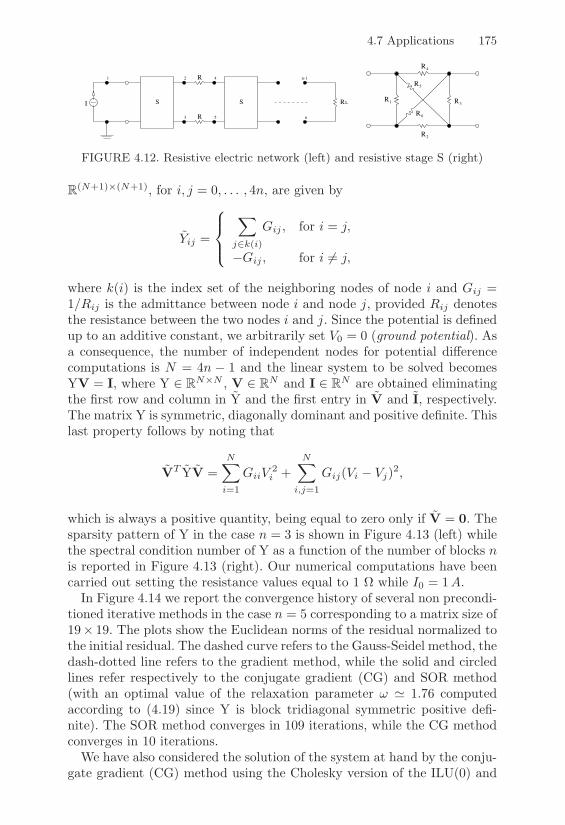
4.7 Applications 175
R
I S S
R
RL
2 41
3 5 n
n-1
6
R
RR
R
R
R
1
2
3
4
5
FIGURE 4.12. Resistive electric network (left) and resistive stage S (right)
R(N+1)!(N+1), for i, j = 0, . . . , 4n, are given by
Yij =
)*+
*,
(
j#k(i)
Gij , for i = j,
"Gij , for i '= j,
where k(i) is the index set of the neighboring nodes of node i and Gij =1/Rij is the admittance between node i and node j, provided Rij denotesthe resistance between the two nodes i and j. Since the potential is definedup to an additive constant, we arbitrarily set V0 = 0 (ground potential). Asa consequence, the number of independent nodes for potential di!erencecomputations is N = 4n " 1 and the linear system to be solved becomesYV = I, where Y ! RN!N , V ! RN and I ! RN are obtained eliminatingthe first row and column in Y and the first entry in V and I, respectively.The matrix Y is symmetric, diagonally dominant and positive definite. Thislast property follows by noting that
VT YV =N(
i=1
GiiV2i +
N(
i,j=1
Gij(Vi " Vj)2,
which is always a positive quantity, being equal to zero only if V = 0. Thesparsity pattern of Y in the case n = 3 is shown in Figure 4.13 (left) whilethe spectral condition number of Y as a function of the number of blocks nis reported in Figure 4.13 (right). Our numerical computations have beencarried out setting the resistance values equal to 1 ( while I0 = 1A.
In Figure 4.14 we report the convergence history of several non precondi-tioned iterative methods in the case n = 5 corresponding to a matrix size of19% 19. The plots show the Euclidean norms of the residual normalized tothe initial residual. The dashed curve refers to the Gauss-Seidel method, thedash-dotted line refers to the gradient method, while the solid and circledlines refer respectively to the conjugate gradient (CG) and SOR method(with an optimal value of the relaxation parameter 0 1 1.76 computedaccording to (4.19) since Y is block tridiagonal symmetric positive defi-nite). The SOR method converges in 109 iterations, while the CG methodconverges in 10 iterations.
We have also considered the solution of the system at hand by the conju-gate gradient (CG) method using the Cholesky version of the ILU(0) and

176 4. Iterative Methods for Solving Linear Systems
0 2 4 6 8 10 12
0
2
4
6
8
10
120 5 10 15 20 25 30 35 40 45 50
100
101
102
103
104
105
FIGURE 4.13. Sparsity pattern of Y for n = 3 (left) and spectral conditionnumber of Y as a function of n (right)
0 50 100 150 200 25010
!16
10!14
10!12
10!10
10!8
10!6
10!4
10!2
100
102
FIGURE 4.14. Convergence history of several non preconditioned iterative meth-ods
MILU(0) preconditioners, where drop tolerances equal to + = 10"2, 10"3
have been chosen for the MILU(0) preconditioner (see Section 4.3.2). Cal-culations with both preconditioners have been done using the MATLABfunctions cholinc and michol. Table 4.2 shows the convergence iterationsof the method for n = 5, 10, 20, 40, 80, 160 and for the considered values of+. We report in the second column the number of nonzero entries in theCholesky factor of matrix Y, in the third column the number of iterationsfor the CG method without preconditioning to converge, while the columnsICh(0) and MICh(0) with + = 10"2 and + = 10"3 show the same infor-mation for the CG method using the incomplete Cholesky and modifiedincomplete Cholesky preconditioners, respectively.The entries in the table are the number of iterations to converge and thenumber in the brackets are the nonzero entries of the L-factor of the cor-responding preconditioners. Notice the decrease of the iterations as + de-creases, as expected. Notice also the increase of the number of iterationswith respect to the increase of the size of the problem.
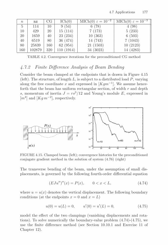
4.7 Applications 177
n nz CG ICh(0) MICh(0) + = 10"2 MICh(0) + = 10"3
5 114 10 9 (54) 6 (78) 4 (98)10 429 20 15 (114) 7 (173) 5 (233)20 1659 40 23 (234) 10 (363) 6 (503)40 6519 80 36 (474) 14 (743) 7 (1043)80 25839 160 62 (954) 21 (1503) 10 (2123)160 102879 320 110 (1914) 34 (3023) 14 (4283)
TABLE 4.2. Convergence iterations for the preconditioned CG method
4.7.2 Finite Di!erence Analysis of Beam BendingConsider the beam clamped at the endpoints that is drawn in Figure 4.15(left). The structure, of length L, is subject to a distributed load P , varyingalong the free coordinate x and expressed in [Kgm"1]. We assume hence-forth that the beam has uniform rectangular section, of width r and depths, momentum of inertia J = rs3/12 and Young’s module E, expressed in[m4] and [Kgm"2], respectively.
P(x)
u(x)
x
0 20 40 60 80 100 12010
!20
10!15
10!10
10!5
100
105
n=10 n=60 n=110
FIGURE 4.15. Clamped beam (left); convergence histories for the preconditionedconjugate gradient method in the solution of system (4.76) (right)
The transverse bending of the beam, under the assumption of small dis-placements, is governed by the following fourth-order di!erential equation
(EJu**)**(x) = P (x), 0 < x < L, (4.74)
where u = u(x) denotes the vertical displacement. The following boundaryconditions (at the endpoints x = 0 and x = L)
u(0) = u(L) = 0, u*(0) = u*(L) = 0, (4.75)
model the e!ect of the two clampings (vanishing displacements and rota-tions). To solve numerically the boundary-value problem (4.74)-(4.75), weuse the finite di!erence method (see Section 10.10.1 and Exercise 11 ofChapter 12).

178 4. Iterative Methods for Solving Linear Systems
With this aim, let us introduce the discretization nodes xj = jh, withh = L/Nh and j = 0, . . . , Nh, and substitute at each node xj the fourth-order derivative with an approximation through centered finite di!erences.Letting f(x) = P (x)/(EJ), fj = f(xj) and denoting by -j the (approx-imate) nodal displacement of the beam at node xj , the finite di!erencediscretization of (4.74)-(4.75) is
B-j"2 " 4-j"1 + 6-j " 4-j+1 + -j+2 = h4fj , #j = 2, . . . , Nh " 2,
-0 = -1 = -Nh"1 = -Nh = 0.(4.76)
The null displacement boundary conditions in (4.76) that have been im-posed at the first and the last two nodes of the grid, require that Nh ) 4.Notice that a fourth-order scheme has been used to approximate the fourth-order derivative, while, for sake of simplicity, a first-order approximationhas been employed to deal with the boundary conditions (see Section10.10.1).
The Nh " 3 discrete equations (4.76) yield a linear system of the formAx = b where the unknown vector x ! RNh"3 and the load vectorb ! RNh"3 are given respectively by x = (-2, -3, . . . , -Nh"2)T and b =(f2, f3, . . . , fNh"2)T , while the coe"cient matrix A ! R(Nh"3)!(Nh"3) ispentadiagonal and symmetric, given by A = pentadiagNh"3(1,"4, 6,"4, 1).
The matrix A is symmetric and positive definite. Therefore, to solvesystem Ax = b, the SSOR preconditioned conjugated gradient method (seeSection 4.21) and the Cholesky factorization method have been employed.In the remainder of the section, the two methods are identified by thesymbols (CG) and (CH).
The convergence histories of CG are reported in Figure 4.15 (right),where the sequences +r(k)+2/+b(k)+2, for the values n = 10, 60, 110, areplotted, r(k) = b " Ax(k) being the residual at the k-th step. The resultshave been obtained using Program 20, with toll=10"15 and 0 = 1.8 in(4.22). The initial vector x(0) has been set equal to the null vector.As a comment to the graphs, it is worth noting that CG has required 7, 33and 64 iterations to converge, respectively, with a maximum absolute errorof 5 ·10"15 with respect to the solution produced by CH. This latter has anoverall computational cost of 136, 1286 and 2436 flops respectively, to becompared with the corresponding 3117, 149424 and 541647 flops of methodCG. As for the performances of the SSOR preconditioner, we remark thatthe spectral condition number of matrix A is equal to 192, 3.8 · 105 and4.5 · 106, respectively, while the corresponding values in the preconditionedcase are 65, 1.2 · 104 and 1.3 · 105.

4.8 Exercises 179
4.8 Exercises1. The spectral radius of the matrix
B =-
a 40 a
.
is %(B) = a. Check that if 0 < a < 1, then %(B) < 1, while &Bm&1/m2 canbe greater than 1.
2. Let A / Rn&n be a strictly diagonally dominant matrix by rows. Showthat the Gauss-Seidel method for the solution of the linear system (3.2) isconvergent.
3. Check that the matrix A = tridiag(%1,$,%1), with $ / R, has eigenvaluesgiven by
#j = $% 2 cos(j.), j = 1, . . . , n
where . = +/(n + 1) and the corresponding eigenvectors are
qj = [sin(j.), sin(2j.), . . . , sin(nj.)]T .
Under which conditions on $ is the matrix positive definite?[Solution : $ ! 2.]
4. Consider the pentadiagonal matrix A = pentadiagn(%1,%1, 10,%1,%1).Assume n = 10 and A = M + N + D, with D = diag(8, . . . , 8) / R10&10,M = pentadiag10(%1,%1, 1, 0, 0) and N = MT . To solve Ax = b, analyzethe convergence of the following iterative methods
(a) (M + D)x(k+1) = %Nx(k) + b,
(b) Dx(k+1) = %(M + N)x(k) + b,
(c) (M + N)x(k+1) = %Dx(k) + b.
[Solution : denoting respectively by %a, %b and %c the spectral radii of theiteration matrices of the three methods, we have %a = 0.1450, %b = 0.5and %c = 12.2870 which implies convergence for methods (a) and (b) anddivergence for method (c).]
5. For the solution of the linear system Ax = b with
A =-
1 22 3
., b =
-35
.,
consider the following iterative method
x(k+1) = B(.)x(k) + g(.), k ! 0, with x(0) given,
where . is a real parameter and
B(.) =14
-2.2 + 2. + 1 %2.2 + 2. + 1%2.2 + 2. + 1 2.2 + 2. + 1
., g(.) =
- 12 % .12 % .
..

180 4. Iterative Methods for Solving Linear Systems
Check that the method is consistent ) . / R. Then, determine the valuesof . for which the method is convergent and compute the optimal valueof . (i.e., the value of the parameter for which the convergence rate ismaximum).[Solution : the method is convergent i" %1 < . < 1/2 and the convergencerate is maximum if . = (1%
'3)/2.]
6. To solve the following block linear system-
A1 BB A2
. -xy
.=
-b1
b2
.,
consider the two methods
(1) A1x(k+1) + By(k) = b1, Bx(k) + A2y(k+1) = b2;
(2) A1x(k+1) + By(k) = b1, Bx(k+1) + A2y(k+1) = b2.
Find su!cient conditions in order for the two schemes to be convergent forany choice of the initial data x(0), y(0).[Solution : method (1) is a decoupled system in the unknowns x(k+1) andy(k+1). Assuming that A1 and A2 are invertible, method (1) converges if%(A%1
1 B) < 1 and %(A%12 B) < 1. In the case of method (2) we have a coupled
system to solve at each step in the unknowns x(k+1) and y(k+1). Solvingformally the first equation with respect to x(k+1) (which requires A1 to beinvertible) and substituting into the second one we see that method (2) isconvergent if %(A%1
2 BA%11 B) < 1 (again A2 must be invertible).]
7. Consider the linear system Ax = b with
A =
"
####$
62 24 1 8 1523 50 7 14 164 6 58 20 2210 12 19 66 311 18 25 2 54
%
&&&&', b =
"
####$
110110110110110
%
&&&&'.
(1) Check if the Jacobi and Gauss-Seidel methods can be applied to solvethe system. (2) Check if the stationary Richardson method with optimalparameter can be applied with P = I and P = D, where D is the diagonalpart of A, and compute the corresponding values of $opt and %opt.[Solution : (1): matrix A is neither diagonally dominant nor symmetricpositive definite, so that we must compute the spectral radii of the itera-tion matrices of the Jacobi and Gauss-Seidel methods to verify if they areconvergent. It turns out that %J = 0.9280 and %GS = 0.3066 which impliesconvergence for both methods. (2): in the case P = I all the eigenvaluesof A are positive so that the Richardson method can be applied yielding$opt = 0.015 and %opt = 0.6452. If P = D the method is still applicableand $opt = 0.8510, %opt = 0.6407.]
8. Consider the linear system Ax = b with
A =
"
##$
5 7 6 57 10 8 76 8 10 95 7 9 10
%
&&' , b =
"
##$
23323331
%
&&' .

4.8 Exercises 181
Analyze the convergence properties of the Jacobi and Gauss-Seidel methodsapplied to the system above in their point and block forms (for a 212 blockpartition of A).[Solution : both methods are convergent, the block form being the fasterone. Moreover, %2(BJ) = %(BGS).]
9. To solve the linear system Ax = b, consider the iterative method (4.6),with P = D + -F and N = %)F% E, - and ) being real numbers. Checkthat the method is consistent only if ) = 1 % -. In such a case, expressthe eigenvalues of the iteration matrix as a function of - and determine forwhich values of - the method is convergent, as well as the value of -opt,assuming that A = tridiag10(%1, 2,%1).[Hint : Take advantage of the result in Exercise 3.]
10. Let A / Rn&n be such that A = (1+-)P%(N+-P), with P%1N nonsingularand with real eigenvalues 1 > #1 ! #2 ! . . . ! #n. Find the values of - / R
for which the following iterative method
(1 + -)Px(k+1) = (N + -P)x(k) + b, k ! 0,
converges )x(0) to the solution of the linear system (3.2). Determine alsothe value of - for which the convergence rate is maximum.[Solution : - > %(1 + #n)/2; -opt = %(#1 + #n)/2.]
11. Consider the linear system
Ax = b with A =-
3 22 6
., b =
-2
%8
..
Write the associated functional %(x) and give a graphical interpretation ofthe solution of the linear system. Perform some iterations of the gradientmethod, after proving convergence for it.
12. Check that in the gradient method x(k+2) is not an optimal direction withrespect to r(k).
13. Show that the coe!cients $k and )k in the conjugate gradient method canbe written in the alternative form (4.45).[Solution: notice Ap(k) = (r(k) % r(k+1))/$k and thus (Ap(k))T r(k+1) =%&r(k+1)&22/$k. Moreover, $k(Ap(k))Tp(k) = %&r(k)&22.]
14. Prove the three-terms recursive relation (4.46) for the residual in the con-jugate gradient method.[Solution: subtract from both sides of Ap(k) = (r(k)%r(k+1))/$k the quan-tity )k%1/$kr(k) and recall that Ap(k) = Ar(k) % )k%1Ap(k%1). Then, ex-pressing the residual r(k) as a function of r(k%1) one immediately gets thedesired relation.]
5Approximation of Eigenvalues andEigenvectors
In this chapter we deal with approximations of the eigenvalues and eigen-vectors of a matrix A ! Cn!n. Two main classes of numerical methodsexist to this purpose, partial methods, which compute the extremal eigen-values of A (that is, those having maximum and minimum module), orglobal methods, which approximate the whole spectrum of A.It is worth noting that methods which are introduced to solve the matrixeigenvalue problem are not necessarily suitable for calculating the matrixeigenvectors. For example, the power method (a partial method, see Section5.3) provides an approximation to a particular eigenvalue/eigenvector pair.
The QR method (a global method, see Section 5.5) instead computes thereal Schur form of A, a canonical form that displays all the eigenvalues ofA but not its eigenvectors. These eigenvectors can be computed, startingfrom the real Schur form of A, with an extra amount of work, as describedin Section 5.8.2.
Finally, some ad hoc methods for dealing e!ectively with the special casewhere A is a symmetric (n% n) matrix are considered in Section 5.10.
5.1 Geometrical Location of the Eigenvalues
Since the eigenvalues of A are the roots of the characteristic polynomialpA($) (see Section 1.7), iterative methods must be used for their approxi-mation when n ) 5. Knowledge of eigenvalue location in the complex planecan thus be helpful in accelerating the convergence of the process.

184 5. Approximation of Eigenvalues and Eigenvectors
A first estimate is provided by Theorem 1.4,
|$| & +A+, #$ ! ((A), (5.1)
for any consistent matrix norm + · +. Inequality (5.1), which is often quiterough, states that all the eigenvalues of A are contained in a circle of radiusR)A) = +A+ centered at the origin of the Gauss plane.Another result is obtained by extending the Decomposition Property 1.23to complex-valued matrices.
Theorem 5.1 If A ! Cn!n, let
H =8A + AH
9/2 and iS =
8A"AH
9/2
be the hermitian and skew-hermitian parts of A, respectively, i being theimaginary unit. For any $ ! ((A)
$min(H) & Re($) & $max(H), $min(S) & Im($) & $max(S). (5.2)
Proof. From the definition of H and S it follows that A = H + iS. Let u / Cn,&u&2 = 1, be the eigenvector associated with the eigenvalue #; the Rayleighquotient (introduced in Section 1.7) reads
# = uHAu = uHHu + iuHSu. (5.3)
Notice that both H and S are hermitian matrices, whilst iS is skew-hermitian.Matrices H and S are thus unitarily similar to a real diagonal matrix (see Section1.7), and therefore their eigenvalues are real. In such a case, (5.3) yields
Re(#) = uHHu, Im(#) = uHSu,
from which (5.2) follows. !
An a priori bound for the eigenvalues of A is given by the following result.
Theorem 5.2 (of the Gershgorin circles) Let A ! Cn!n. Then
((A) 7 SR =nT
i=1
Ri, Ri = {z ! C : |z " aii| &n(
j=1j '=i
|aij |}. (5.4)
The sets Ri are called Gershgorin circles.
Proof. Let us decompose A as A = D + E, where D is the diagonal part ofA, whilst eii = 0 for i = 1, . . . , n. For # / '(A) (with # $= aii, i = 1, . . . , n),let us introduce the matrix B% = A % #I = (D % #I) + E. Since B% is singular,there exists a non-null vector x / Cn such that B%x = 0. This means that((D% #I) + E)x = 0, that is, passing to the & · &! norm,
x = %(D% #I)%1Ex, &x&! " &(D% #I)%1E&!&x&!,
5.1 Geometrical Location of the Eigenvalues 185
and thus
1 " &(D% #I)%1E&! =n(
j=1
|ekj ||akk % #| =
n(
j=1j #=k
|akj ||akk % #| (5.5)
for a certain k, 1 " k " n. Inequality (5.5) implies # / Rk and thus (5.4). !
The bounds (5.4) ensure that any eigenvalue of A lies within the unionof the circles Ri. Moreover, since A and AT share the same spectrum,Theorem 5.2 also holds in the form
((A) 7 SC =nT
j=1
Cj , Cj = {z ! C : |z " ajj | &n(
i=1i '=j
|aij |}. (5.6)
The circles Ri in the complex plane are called row circles, and Cj columncircles. The immediate consequence of (5.4) and (5.6) is the following.
Property 5.1 (First Gershgorin theorem) For a given matrix A !Cn!n,
#$ ! ((A), $ ! SRU
SC . (5.7)
The following two location theorems can also be proved (see [Atk89], pp.588-590 and [Hou75], pp. 66-67).
Property 5.2 (Second Gershgorin theorem) Let
S1 =mT
i=1
Ri, S2 =nT
i=m+1
Ri.
If S18S2 = 9, then S1 contains exactly m eigenvalues of A, each one beingaccounted for with its algebraic multiplicity, while the remaining eigenvaluesare contained in S2.
Remark 5.1 Properties 5.1 and 5.2 do not exclude the possibility thatthere exist circles containing no eigenvalues, as happens for the matrix inExercise 1. !
Definition 5.1 A matrix A ! Cn!n is called reducible if there exists apermutation matrix P such that
PAPT =
NB11 B12
0 B22
O
,
where B11 and B22 are square matrices; A is irreducible if it is not reducible.!

186 5. Approximation of Eigenvalues and Eigenvectors
To check if a matrix is reducible, the oriented graph of the matrix can beconveniently employed. Recall from Section 3.9 that the oriented graph of areal matrix A is obtained by joining n points (called vertices of the graph)P1, . . . , Pn through a line oriented from Pi to Pj if the correspondingmatrix entry aij '= 0. An oriented graph is strongly connected if for anypair of distinct vertices Pi and Pj there exists an oriented path from Pi toPj . The following result holds (see [Var62] for the proof).
Property 5.3 A matrix A ! Rn!n is irreducible i! its oriented graph isstrongly connected.
Property 5.4 (Third Gershgorin theorem) Let A ! Cn!n be an irre-ducible matrix. An eigenvalue $ ! ((A) cannot lie on the boundary of SRunless it belongs to the boundary of every circle Ri, for i = 1, . . . , n.
Example 5.1 Let us consider the matrix
A =
"
##$
10 2 3
%1 2 %1
0 1 3
%
&&'
whose spectrum is (to four significant figures) '(A) = {9.687, 2.656±i0.693}. Thefollowing values of the norm of A: &A&1 = 11, &A&2 = 10.72, &A&! = 15 and&A&F = 11.36 can be used in the estimate (5.1). Estimate (5.2) provides instead1.96 " Re(#(A)) " 10.34, %2.34 " Im(#(A)) " 2.34, while the row and columncircles are given respectively by R1 = {|z| : |z%10| " 5}, R2 = {|z| : |z%2| " 2},R3 = {|z| : |z % 3| " 1} and C1 = {|z| : |z % 10| " 1}, C2 = {|z| : |z % 2| " 3},C3 = {|z| : |z % 3| " 4}.In Figure 5.1, for i = 1, 2, 3 the Ri and Ci circles and the intersection SR . SC(shaded areas) are drawn. In agreement with Property 5.2, we notice that aneigenvalue is contained in C1, which is disjoint from C2 and C3, while the remainingeigenvalues, thanks to Property 5.1, lie within the set R2 4 {C3 .R1}. •
5.2 Stability and Conditioning Analysis
In this section we introduce some a priori and a posteriori estimates thatare relevant in the stability analysis of the matrix eigenvalue and eigenvec-tor problem. The presentation follows the guidelines that have been tracedin Chapter 2.
5.2.1 A priori EstimatesAssume that A ! Cn!n is a diagonalizable matrix and denote by X =(x1, . . . ,xn) ! Cn!n the matrix of its right eigenvectors, where xk ! Cn
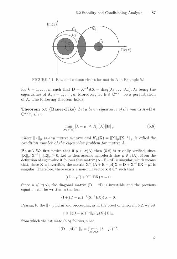
5.2 Stability and Conditioning Analysis 187
2 Re(z)3 10
C3
C2
C1R3R2
R1
Im(z)
FIGURE 5.1. Row and column circles for matrix A in Example 5.1
for k = 1, . . . , n, such that D = X"1AX = diag($1, . . . ,$n), $i being theeigenvalues of A, i = 1, . . . , n. Moreover, let E ! Cn!n be a perturbationof A. The following theorem holds.
Theorem 5.3 (Bauer-Fike) Let µ be an eigenvalue of the matrix A+E !Cn!n; then
min##$(A)
|$" µ| & Kp(X)+E+p (5.8)
where + · +p is any matrix p-norm and Kp(X) = +X+p+X"1+p is called thecondition number of the eigenvalue problem for matrix A.
Proof. We first notice that if µ / '(A) then (5.8) is trivially verified, since&X&p&X%1&p&E&p ! 0. Let us thus assume henceforth that µ $/ '(A). From thedefinition of eigenvalue it follows that matrix (A+E%µI) is singular, which meansthat, since X is invertible, the matrix X%1(A + E % µI)X = D + X%1EX % µI issingular. Therefore, there exists a non-null vector x / Cn such that
8(D% µI) + X%1EX
9x = 0.
Since µ $/ '(A), the diagonal matrix (D % µI) is invertible and the previousequation can be written in the form
8I + (D% µI)%1(X%1EX)
9x = 0.
Passing to the & · &p norm and proceeding as in the proof of Theorem 5.2, we get
1 " &(D% µI)%1&pKp(X)&E&p,
from which the estimate (5.8) follows, since
&(D% µI)%1&p = ( min%'&(A)
|#% µ|)%1.
!

188 5. Approximation of Eigenvalues and Eigenvectors
If A is a normal matrix, from the Schur decomposition theorem (see Section1.8) it follows that the similarity transformation matrix X is unitary so thatKp(X) = 1. This implies that
#µ ! ((A + E), min##$(A)
|$" µ| & +E+p, (5.9)
hence the eigenvalue problem is well-conditioned with respect to the abso-lute error. This, however, does not prevent the matrix eigenvalue problemfrom being a!ected by significant relative errors, especially when A has awidely spread spectrum.
Example 5.2 Let us consider, for 1 " n " 10, the calculation of the eigenvaluesof the Hilbert matrix Hn / Rn&n (see Example 3.2, Chapter 3). It is symmetric(thus, in particular, normal) and exhibits, for n ! 4, a very large conditionnumber. Let En / Rn&n be a matrix having constant entries equal to 0 = 10%3.We show in Table 5.1 the results of the computation of the minimum in (5.9),taking p = 2 (that is, &En&2 = n0). Notice how the absolute error is decreasing,since the eigenvalue of minimum module tends to zero, whilst the relative erroris increasing as the size n of the matrix increases, due to the higher sensitivity of“small” eigenvalues with respect to rounding errors. •
n Abs. Err. Rel. Err. +En+2 K2(Hn) K2(Hn + En)1 1 · 10"3 1 · 10"3 1 · 10"3 1 · 10"3 12 1.677 · 10"4 1.446 · 10"3 2 · 10"3 19.28 19.264 5.080 · 10"7 2.207 · 10"3 4 · 10"3 1.551 · 104 1.547 · 104
8 1.156 · 10"12 3.496 · 10"3 8 · 10"3 1.526 · 1010 1.515 · 1010
10 1.355 · 10"15 4.078 · 10"3 1 · 10"2 1.603 · 1013 1.589 · 1013
TABLE 5.1. Relative and absolute errors in the calculation of the eigenvalues ofthe Hilbert matrix (using the MATLAB intrinsic function eig). “Abs. Err.” and“Rel. Err.” denote respectively the absolute and relative errors (with respect to#)
The Bauer-Fike theorem states that the matrix eigenvalue problem is well-conditioned if A is a normal matrix. Failure to fulfil this property, however,does not necessarily imply that A must exhibit a “strong” numerical sen-sitivity to the computation of every one of its eigenvalues. In this respect,the following result holds, which can be regarded as an a priori estimate ofthe conditioning of the calculation of a particular eigenvalue of a matrix.
Theorem 5.4 Let A ! Cn!n be a diagonalizable matrix; let $, x and ybe a simple eigenvalue of A and its associated right and left eigenvectors,respectively, with +x+2 = +y+2 = 1. Moreover, for + > 0, let A(+) =A+ +E, with E ! Cn!n such that +E+2 = 1. Denoting by $(+) and x(+) the

5.2 Stability and Conditioning Analysis 189
eigenvalue and the corresponding eigenvector of A(+), such that $(0) = $and x(0) = x,
>>>>.$
.+(0)
>>>> &1
|yHx| . (5.10)
Proof. Let us first prove that yHx $= 0. Setting Y = (y1, . . . ,yn) = (XH)%1,with yk / Cn for k = 1, . . . , n, it follows that yH
k A = #kyHk , i.e., the rows
of X%1 = YH are left eigenvectors of A. Then, since YHX = I, yHi xj = !ij
for i, j = 1, . . . , n, !ij being the Kronecker symbol. This result is equivalent tosaying that the eigenvectors {x} of A and the eigenvectors {y} of AH form abi-orthogonal set (see (4.67)).
Let us now prove (5.10). Since the roots of the characteristic equation arecontinuous functions of the coe!cients of the characteristic polynomial associatedwith A(&), it follows that the eigenvalues of A(&) are continuous functions of &(see, for instance, [Hen74], p. 281). Therefore, in a neighborhood of & = 0,
(A + &E)x(&) = #(&)x(&).
Di"erentiating the previous equation with respect to & and setting & = 0 yields
A1x1&
(0) + Ex =1#1&
(0)x + #1x1&
(0),
from which, left-multiplying both sides by yH and recalling that yH is a lefteigenvector of A,
1#1&
(0) =yHExyHx
.
Using the Cauchy-Schwarz inequality gives the desired estimate (5.10). !
Notice that |yHx| = | cos(!#)|, where !# is the angle between the eigenvec-tors yH and x (both having unit Euclidean norm). Therefore, if these twovectors are almost orthogonal the computation of the eigenvalue $ turnsout to be ill-conditioned. The quantity
2($) =1
|yHx| =1
| cos(!#)| (5.11)
can thus be taken as the condition number of the eigenvalue $. Obviously,2($) ) 1; when A is a normal matrix, since it is unitarily similar to adiagonal matrix, the left and right eigenvectors y and x coincide, yielding2($) = 1/+x+22 = 1.
Inequality (5.10) can be roughly interpreted as stating that perturbationsof the order of %+ in the entries of matrix A induce changes of the order of%$ = %+/| cos(!#)| in the eigenvalue $. If normal matrices are considered,the calculation of $ is a well-conditioned problem; the case of a generic non-symmetric matrix A can be conveniently dealt with using methods basedon similarity transformations, as will be seen in later sections.
190 5. Approximation of Eigenvalues and Eigenvectors
It is interesting to check that the conditioning of the matrix eigenvalueproblem remains unchanged if the transformation matrices are unitary. Tothis end, let U ! Cn!n be a unitary matrix and let DA = UHAU. Also let$j be an eigenvalue of A and denote by 2j the condition number (5.11).Moreover, let D2j be the condition number of $j when it is regarded as aneigenvalue of DA. Finally, let {xk}, {yk} be the right and left eigenvectors ofA respectively. Clearly, {UHxk}, {UHyk} are the right and left eigenvectorsof DA. Thus, for any j = 1, . . . , n,
D2j =>>yH
j UUHxj
>>"1= 2j ,
from which it follows that the stability of the computation of $j is nota!ected by performing similarity transformations using unitary matrices.It can also be checked that unitary transformation matrices do not changethe Euclidean length and the angles between vectors in Cn. Moreover, thefollowing a priori estimate holds (see [GL89], p. 317)
fl8X"1AX
9= X"1AX + E, with +E+2 1 uK2(X)+A+2 (5.12)
where fl(M) is the machine representation of matrix M and u is the roundo!unit (see Section 2.5). From (5.12) it follows that using nonunitary trans-formation matrices in the eigenvalue computation can lead to an unstableprocess with respect to rounding errors.We conclude this section with a stability result for the approximation ofthe eigenvector associated with a simple eigenvalue. Under the same as-sumptions of Theorem 5.4, the following result holds (see for the proof,[Atk89], Problem 6, pp. 649-650).
Property 5.5 The eigenvectors xk and xk(+) of the matrices A and A(+) =A + +E, with +xk(+)+2 = +xk+2 = 1 for k = 1, . . . , n, satisfy
+xk(+)" xk+2 &+
minj '=k |$k " $j |+E+2 + O(+2), #k = 1, . . . , n.
Analogous to (5.11), the quantity
2(xk) =1
minj '=k |$k " $j |
can be regarded as being the condition number of the eigenvector xk. Com-puting xk might be an ill-conditioned operation if some eigenvalues $j are“very close” to the eigenvalue $k associated with xk.
5.2.2 A posteriori EstimatesThe a priori estimates examined in the previous section characterize thestability properties of the matrix eigenvalue and eigenvector problem. From

5.2 Stability and Conditioning Analysis 191
the implementation standpoint, it is also important to dispose of a pos-teriori estimates that allow for a run-time control of the quality of theapproximation that is being constructed. Since the methods that will beconsidered later are iterative processes, the results of this section can beusefully employed to devise reliable stopping criteria for these latter.
Theorem 5.5 Let A ! Cn!n be an hermitian matrix and let (:$, :x) bethe computed approximations of an eigenvalue/eigenvector pair ($,x) ofA. Defining the residual as
:r = A:x" :$:x, :x '= 0,
it then follows that
min#i#$(A)
|:$" $i| &+:r+2+:x+2
. (5.13)
Proof. Since A is hermitian, it admits a system of orthonormal eigenvectors {uk}
which can be taken as a basis of Cn. In particular, :x =n(
i=1
$iui with $i = uHi :x,
and thus :r =n(
i=1
$i(#i % :#)ui. As a consequence
4&:r&2&:x&2
52
=n(
i=1
)i(#i % :#)2, with )i = |$k|2/(n(
j=1
|$j |2). (5.14)
Sincen(
i=1
)i = 1, the inequality (5.13) immediately follows from (5.14). !
The estimate (5.13) ensures that a small absolute error corresponds to asmall relative residual in the computation of the eigenvalue of the matrixA which is closest to :$.Let us now consider the following a posteriori estimate for the eigenvector:x (for the proof, see [IK66], pp. 142-143).
Property 5.6 Under the same assumptions of Theorem 5.5, suppose that|$i " :$| & +:r+2 for i = 1, . . . ,m and that |$i " :$| ) % > 0 for i =m + 1, . . . , n. Then
d(:x,Um) & +:r+2%
(5.15)
where d(:x,Um) is the Euclidean distance between :x and the space Um gen-erated by the eigenvectors ui, i = 1, . . . ,m associated with the eigenvalues$i of A.
192 5. Approximation of Eigenvalues and Eigenvectors
Notice that the a posteriori estimate (5.15) ensures that a small absoluteerror corresponds to a small residual in the approximation of the eigenvec-tor associated with the eigenvalue of A that is closest to :$, provided thatthe eigenvalues of A are well-separated (that is, if % is su"ciently large).In the general case of a nonhermitian matrix A, an a posteriori estimatecan be given for the eigenvalue :$ only when the matrix of the eigenvectorsof A is available. We have the following result (for the proof, we refer to[IK66], p. 146).
Property 5.7 Let A ! Cn!n be a diagonalizable matrix, with matrix ofeigenvectors X = [x1, . . . ,xn]. If, for some + > 0,
+:r+2 & ++:x+2,
thenmin
#i#$(A)|:$" $i| & ++X"1+2+X+2.
This estimate is of little practical use, since it requires the knowledge of allthe eigenvectors of A. Examples of a posteriori estimates that can actuallybe implemented in a numerical algorithm will be provided in Sections 5.3.1and 5.3.2.
5.3 The Power Method
The power method is very good at approximating the extremal eigenvaluesof the matrix, that is, the eigenvalues having largest and smallest module,denoted by $1 and $n respectively, as well as their associated eigenvectors.
Solving such a problem is of great interest in several real-life applications(geosysmic, machine and structural vibrations, electric network analysis,quantum mechanics, . . . ) where the computation of $n (and its associatedeigenvector xn) arises in the determination of the proper frequency (andthe corresponding fundamental mode) of a given physical system. We shallcome back to this point in Section 5.12.
Having approximations of $1 and $n can also be useful in the analysis ofnumerical methods. For instance, if A is symmetric and positive definite,one can compute the optimal value of the acceleration parameter of theRichardson method and estimate its error reducing factor (see Chapter4), as well as perform the stability analysis of discretization methods forsystems of ordinary di!erential equations (see Chapter 11).
5.3.1 Approximation of the Eigenvalue of Largest ModuleLet A ! Cn!n be a diagonalizable matrix and let X ! Cn!n be the matrix ofits eigenvectors xi, for i = 1, . . . , n. Let us also suppose that the eigenvalues

5.3 The Power Method 193
of A are ordered as
|$1| > |$2| ) |$3| . . . ) |$n|, (5.16)
where $1 has algebraic multiplicity equal to 1. Under these assumptions,$1 is called the dominant eigenvalue of matrix A.Given an arbitrary initial vector q(0) ! Cn of unit Euclidean norm, considerfor k = 1, 2, . . . the following iteration based on the computation of powersof matrices, commonly known as the power method:
z(k) = Aq(k"1)
q(k) = z(k)/+z(k)+23(k) = (q(k))HAq(k).
(5.17)
Let us analyze the convergence properties of method (5.17). By inductionon k one can check that
q(k) =Akq(0)
+Akq(0)+2, k ) 1. (5.18)
This relation explains the role played by the powers of A in the method.Because A is diagonalizable, its eigenvectors xi form a basis of Cn; it isthus possible to represent q(0) as
q(0) =n(
i=1
"ixi, "i ! C, i = 1, . . . , n. (5.19)
Moreover, since Axi = $ixi, we have
Akq(0) = "1$k1
6
x1 +n(
i=2
"i
"1
4$i$1
5k
xi
7
, k = 1, 2, . . . (5.20)
Since |$i/$1| < 1 for i = 2, . . . , n, as k increases the vector Akq(0) (andthus also q(k), due to (5.18)), tends to assume an increasingly significantcomponent in the direction of the eigenvector x1, while its components inthe other directions xj decrease. Using (5.18) and (5.20), we get
q(k) ="1$k1(x1 + y(k))+"1$k1(x1 + y(k))+2
= µkx1 + y(k)
+x1 + y(k)+2,
where µk is the sign of "1$k1 and y(k) denotes a vector that vanishes ask (,.
As k (,, the vector q(k) thus aligns itself along the direction of eigen-vector x1, and the following error estimate holds at each step k.

194 5. Approximation of Eigenvalues and Eigenvectors
Theorem 5.6 Let A ! Cn!n be a diagonalizable matrix whose eigenvaluessatisfy (5.16). Assuming that "1 '= 0, there exists a constant C > 0 suchthat
+q(k) " x1+2 & C
>>>>$2
$1
>>>>k
, k ) 1, (5.21)
where
q(k) =q(k)+Akq(0)+2
"1$k1= x1 +
n(
i=2
"i
"1
4$i$1
5k
xi, k = 1, 2, . . . (5.22)
Proof. Since A is diagonalizable, without losing generality, we can pick up thenonsingular matrix X in such a way that its columns have unit Euclidean length,that is &xi&2 = 1 for i = 1, . . . , n. From (5.20) it thus follows that
&x1 +n(
i=2
N$i
$1
4#i
#1
5k
xi
O
% x1&2 = &n(
i=2
$i
$1
4#i
#1
5k
xi&2
"6
n(
i=2
-$i
$1
.2 -#i
#1
.2k71/2
">>>>#2
#1
>>>>k
6n(
i=2
-$i
$1
.271/2
,
that is (5.21) with C =
6n(
i=2
($i/$1)271/2
. !
Estimate (5.21) expresses the convergence of the sequence q(k) towards x1.Therefore the sequence of Rayleigh quotients
((q(k))HAq(k))/+q(k)+22 =Kq(k)
LHAq(k) = 3(k)
will converge to $1. As a consequence, limk&$ 3(k) = $1, and the conver-gence will be faster when the ratio |$2/$1| is smaller.
If the matrix A is real and symmetric it can be proved, always assumingthat "1 '= 0, that (see [GL89], pp. 406-407)
|$1 " 3(k)| & |$1 " $n| tan2(!0)>>>>$2
$1
>>>>2k
, (5.23)
where cos(!0) = |xT1 q(0)| '= 0. Inequality (5.23) outlines that the conver-
gence of the sequence 3(k) to $1 is quadratic with respect to the ratio |$2/$1|(we refer to Section 5.3.3 for numerical results).We conclude the section by providing a stopping criterion for the iteration(5.17). For this purpose, let us introduce the residual at step k
r(k) = Aq(k) " 3(k)q(k), k ) 1,
and, for + > 0, the matrix +E(k) = "r(k) Pq(k)QH ! Cn!n with +E(k)+2 = 1.
Since
+E(k)q(k) = "r(k), k ) 1, (5.24)
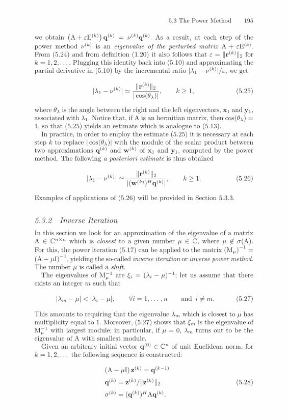
5.3 The Power Method 195
we obtain8A + +E(k)9q(k) = 3(k)q(k). As a result, at each step of the
power method 3(k) is an eigenvalue of the perturbed matrix A + +E(k).From (5.24) and from definition (1.20) it also follows that + = +r(k)+2 fork = 1, 2, . . . . Plugging this identity back into (5.10) and approximating thepartial derivative in (5.10) by the incremental ratio |$1 " 3(k)|/+, we get
|$1 " 3(k)| 1 +r(k)+2| cos(!#)| , k ) 1, (5.25)
where !# is the angle between the right and the left eigenvectors, x1 and y1,associated with $1. Notice that, if A is an hermitian matrix, then cos(!#) =1, so that (5.25) yields an estimate which is analogue to (5.13).
In practice, in order to employ the estimate (5.25) it is necessary at eachstep k to replace | cos(!#)| with the module of the scalar product betweentwo approximations q(k) and w(k) of x1 and y1, computed by the powermethod. The following a posteriori estimate is thus obtained
|$1 " 3(k)| 1 +r(k)+2|(w(k))Hq(k)|
, k ) 1. (5.26)
Examples of applications of (5.26) will be provided in Section 5.3.3.
5.3.2 Inverse IterationIn this section we look for an approximation of the eigenvalue of a matrixA ! Cn!n which is closest to a given number µ ! C, where µ '! ((A).For this, the power iteration (5.17) can be applied to the matrix (Mµ)"1 =(A" µI)"1, yielding the so-called inverse iteration or inverse power method.The number µ is called a shift.
The eigenvalues of M"1µ are *i = ($i " µ)"1; let us assume that there
exists an integer m such that
|$m " µ| < |$i " µ|, #i = 1, . . . , n and i '= m. (5.27)
This amounts to requiring that the eigenvalue $m which is closest to µ hasmultiplicity equal to 1. Moreover, (5.27) shows that *m is the eigenvalue ofM"1
µ with largest module; in particular, if µ = 0, $m turns out to be theeigenvalue of A with smallest module.
Given an arbitrary initial vector q(0) ! Cn of unit Euclidean norm, fork = 1, 2, . . . the following sequence is constructed:
(A" µI) z(k) = q(k"1)
q(k) = z(k)/+z(k)+2((k) = (q(k))HAq(k).
(5.28)

196 5. Approximation of Eigenvalues and Eigenvectors
Notice that the eigenvectors of Mµ are the same as those of A since Mµ =X (%" µIn)X"1, where % = diag($1, . . . ,$n). For this reason, the Rayleighquotient in (5.28) is computed directly on the matrix A (and not on M"1
µ ).The main di!erence with respect to (5.17) is that at each step k a linearsystem with coe"cient matrix Mµ = A" µI must be solved. For numericalconvenience, the LU factorization of Mµ is computed once for all at k = 1,so that at each step only two triangular systems are to be solved, with acost of the order of n2 flops.
Although being more computationally expensive than the power method(5.17), the inverse iteration has the advantage that it can converge to anydesired eigenvalue of A (namely, the one closest to the shift µ). Inverse iter-ation is thus ideally suited for refining an initial estimate µ of an eigenvalueof A, which can be obtained, for instance, by applying the localization tech-niques introduced in Section 5.1. Inverse iteration can be also e!ectivelyemployed to compute the eigenvector associated with a given (approximate)eigenvalue, as described in Section 5.8.1.
In view of the convergence analysis of the iteration (5.28) we assume thatA is diagonalizable, so that q(0) can be represented in the form (5.19).Proceeding in the same way as in the power method, we let
q(k) = xm +n(
i=1,i '=m
"i
"m
4*i*m
5k
xi,
where xi are the eigenvectors of M"1µ (and thus also of A), while "i are as
in (5.19). As a consequence, recalling the definition of *i and using (5.27),we get
limk&$
q(k) = xm, limk&$
((k) = $m.
Convergence will be faster when µ is closer to $m. Under the same assump-tions made for proving (5.26), the following a posteriori estimate can beobtained for the approximation error on $m
|$m " ((k)| 1 +:r(k)+2|(:w(k))Hq(k)|
, k ) 1, (5.29)
where :r(k) = Aq(k) " ((k)q(k) and :w(k) is the k-th iterate of the inversepower method to approximate the left eigenvector associated with $m.
5.3.3 Implementation IssuesThe convergence analysis of Section 5.3.1 shows that the e!ectiveness ofthe power method strongly depends on the dominant eigenvalues beingwell-separated (that is, |$2|/|$1|: 1). Let us now analyze the behavior ofiteration (5.17) when two dominant eigenvalues of equal module exist (thatis, |$2| = |$1|). Three cases must be distinguished:

5.3 The Power Method 197
1. $2 = $1: the two dominant eigenvalues are coincident. The methodis still convergent, since for k su"ciently large (5.20) yields
Akq(0) 1 $k1 ("1x1 + "2x2)
which is an eigenvector of A. For k ( ,, the sequence q(k) (aftera suitable redefinition) converges to a vector lying in the subspacespanned by the eigenvectors x1 and x2, while the sequence 3(k) stillconverges to $1.
2. $2 = "$1: the two dominant eigenvalues are opposite. In this casethe eigenvalue of largest module can be approximated by applying thepower method to the matrix A2. Indeed, for i = 1, . . . , n, $i(A2) =[$i(A)]2, so that $2
1 = $22 and the analysis falls into the previous case,
where the matrix is now A2.
3. $2 = $1: the two dominant eigenvalues are complex conjugate. Here,undamped oscillations arise in the sequence of vectors q(k) and thepower method is not convergent (see [Wil65], Chapter 9, Section 12).
As for the computer implementation of (5.17), it is worth noting that nor-malizing the vector q(k) to 1 keeps away from overflow (when |$1| > 1) orunderflow (when |$1| < 1) in (5.20). We also point out that the requirement"1 '= 0 (which is a priori impossible to fulfil when no information aboutthe eigenvector x1 is available) is not essential for the actual convergenceof the algorithm.
Indeed, although it can be proved that, working in exact arithmetic, thesequence (5.17) converges to the pair ($2,x2) if "1 = 0 (see Exercise 10),the arising of (unavoidable) rounding errors ensures that in practice thevector q(k) contains a non-null component also in the direction of x1. Thisallows for the eigenvalue $1 to “show-up” and the power method to quicklyconverge to it.An implementation of the power method is given in Program 26. Hereand in the following algorithm, the convergence check is based on the aposteriori estimate (5.26).
Here and in the remainder of the chapter, the input data z0, toll andnmax are the initial vector, the tolerance for the stopping test and themaximum admissible number of iterations, respectively. In output, the vec-tors nu1 and err contain the sequences {3(k)} and {+r(k)+2/| cos(!#)|} (see(5.26)), whilst x1 and niter are the approximation of the eigenvector x1and the number of iterations taken by the algorithm to converge, respec-tively.
Program 26 - powerm : Power method
function [nu1,x1,niter,err]=powerm(A,z0,toll,nmax)

198 5. Approximation of Eigenvalues and Eigenvectors
q=z0/norm(z0); q2=q; err=[]; nu1=[]; res=toll+1; niter=0; z=A*q;while (res >= toll & niter <= nmax)q=z/norm(z); z=A*q; lam=q’*z; x1=q;z2=q2’*A; q2=z2/norm(z2); q2=q2’;y1=q2; costheta=abs(y1’*x1);if (costheta >= 5e-2),niter=niter+1; res=norm(z-lam*q)/costheta;err=[err; res]; nu1=[nu1; lam];
elsedisp(’ Multiple eigenvalue ’); break;
endend
A coding of the inverse power method is provided in Program 27. Theinput parameter mu is the initial approximation of the eigenvalue. In output,the vectors sigma and err contain the sequences {((k)} and
/+:r(k)+2/|(:w(k))H
q(k)|0
(see (5.29)). The LU factorization (with partial pivoting) of the ma-trix Mµ is carried out using the MATLAB intrinsic function lu.
Program 27 - invpower : Inverse power method
function [sigma,x,niter,err]=invpower(A,z0,mu,toll,nmax)n=max(size(A)); M=A-mu*eye(n); [L,U,P]=lu(M);q=z0/norm(z0); q2=q’; err=[]; sigma=[]; res=toll+1; niter=0;while (res >= toll & niter <= nmax)niter=niter+1; b=P*q; y=L\b; z=U\y;q=z/norm(z); z=A*q; lam=q’*z;b=q2’; y=U’\b; w=L’\y;q2=(P’*w)’; q2=q2/norm(q2); costheta=abs(q2*q);if (costheta >= 5e-2),
res=norm(z-lam*q)/costheta; err=[err; res]; sigma=[sigma; lam];else,
disp(’ Multiple eigenvalue ’); break;endx=q;end
Example 5.3 The matrix A in (5.30)
A =
"
##$
15 %2 2
1 10 %3
%2 1 0
%
&&' , V =
"
##$
%0.944 0.393 %0.088
%0.312 0.919 0.309
0.112 0.013 0.947
%
&&' (5.30)
has the following eigenvalues (to five significant figures): #1 = 14.103, #2 = 10.385and #3 = 0.512, while the corresponding eigenvectors are the vector columns ofmatrix V.

5.3 The Power Method 199
0 10 20 30 40 50 60 70 8010
!12
10!10
10!8
10!6
10!4
10!2
100
0 6 12 1810
!14
10!12
10!10
10!8
10!6
10!4
10!2
100
(S)
(NS)
FIGURE 5.2. Comparison between the a posteriori error estimate and the actualabsolute error for matrix A in (5.30) (left); convergence curves for the powermethod applied to matrix A in (5.31) in its symmetric (S) and nonsymmetric(NS) forms (right)
To approximate the pair (#1,x1), we have run the Program 26 with initial datumz(0) = (1, 1, 1)T . After 71 iterations of the power method the absolute errors are|#1 % 2(71)| = 7.91 · 10%11 and &x1 % x(71)
1 &! = 1.42 · 10%11.In a second run, we have used z(0) = x2 + x3 (notice that with this choice
$1 = 0). After 215 iterations the absolute errors are |#1 % 2(215)| = 4.26 · 10%14
and &x1 % x(215)1 &! = 1.38 · 10%14.
Figure 5.2 (left) shows the reliability of the a posteriori estimate (5.26). Thesequences |#1 % 2(k)| (solid line) and the corresponding a posteriori estimates(5.26) (dashed line) are plotted as a function of the number of iterations (inabscissae). Notice the excellent agreement between the two curves.
The symmetric matrix A in (5.31)
A =
"
##$
1 3 4
3 1 2
4 2 1
%
&&' , T =
"
##$
8 1 6
3 5 7
4 9 2
%
&&' (5.31)
has the following spectrum: #1 = 7.047, #2 = %3.1879 and #3 = %0.8868 (to fivesignificant figures).It is interesting to compare the behaviour of the power method when computing#1 for the symmetric matrix A and for its similar matrix M = T%1AT, where Tis the nonsingular (and nonorthogonal) matrix in (5.31).Running Program 26 with z(0) = (1, 1, 1)T , the power method converges to theeigenvalue #1 in 18 and 30 iterations, for matrices A and M, respectively. Thesequence of absolute errors |#1 % 2(k)| is plotted in Figure 5.2 (right) where (S)and (NS) refer to the computations on A and M, respectively. Notice the rapiderror reduction in the symmetric case, according to the quadratic convergenceproperties of the power method (see Section 5.3.1).We finally employ the inverse power method (5.28) to compute the eigenvalueof smallest module #3 = 0.512 of matrix A in (5.30). Running Program 27 withq(0) = (1, 1, 1)T /
'3, the method converges in 9 iterations, with absolute errors
|#3 % '(9)| = 1.194 · 10%12 and &x3 % x(9)3 &! = 4.59 · 10%13. •

200 5. Approximation of Eigenvalues and Eigenvectors
5.4 The QR Iteration
In this section we present some iterative techniques for simultaneously ap-proximating all the eigenvalues of a given matrix A. The basic idea consistsof reducing A, by means of suitable similarity transformations, into a formfor which the calculation of the eigenvalues is easier than on the startingmatrix.
The problem would be satisfactorily solved if the unitary matrix U of theSchur decomposition theorem 1.5, such that T = UHAU, T being uppertriangular and with tii = $i(A) for i = 1, . . . , n, could be determined in adirect way, that is, with a finite number of operations. Unfortunately, it isa consequence of Abel’s theorem that, for n ) 5, the matrix U cannot becomputed in an elementary way (see Exercise 8). Thus, our problem canbe solved only resorting to iterative techniques.The reference algorithm in this context is the QR iteration method, that ishere examined only in the case of real matrices. (For some remarks on theextension of the algorithms to the complex case, see [GL89], Section 5.2.10and [Dem97], Section 4.2.1).
Let A ! Rn!n; given an orthogonal matrix Q(0) ! Rn!n and lettingT(0) = (Q(0))TAQ(0), for k = 1, 2, . . . , until convergence, the QR iterationconsists of:
determine Q(k),R(k) such that
Q(k)R(k) = T(k"1) (QR factorization);
then, let
T(k) = R(k)Q(k).
(5.32)
At each step k ) 1, the first phase of the iteration is the factorization ofthe matrix T(k"1) into the product of an orthogonal matrix Q(k) with anupper triangular matrix R(k) (see Section 5.6.3). The second phase is asimple matrix product. Notice that
T(k) = R(k)Q(k) = (Q(k))T (Q(k)R(k))Q(k) = (Q(k))TT(k"1)Q(k)
= (Q(0)Q(1) . . .Q(k))TA(Q(0)Q(1) . . .Q(k)), k ) 0,(5.33)
i.e., every matrix T(k) is orthogonally similar to A. This is particularlyrelevant for the stability of the method, since, as shown in Section 5.2, theconditioning of the matrix eigenvalue problem for T(k) is not worse than itis for A (see also [GL89], p. 360).
A basic implementation of the QR iteration (5.32), assuming Q(0) = In,is examined in Section 5.5, while a more computationally e"cient version,starting from T(0) in upper Hessenberg form, is described in detail in Sec-tion 5.6.

5.5 The Basic QR Iteration 201
If A has real eigenvalues, distinct in module, it will be seen in Section 5.5that the limit of T(k) is an upper triangular matrix (with the eigenvalues ofA on the main diagonal). However, if A has complex eigenvalues the limitof T(k) cannot be an upper triangular matrix T. Indeed if it were T wouldnecessarily have real eigenvalues, although it is similar to A.
Failure to converge to a triangular matrix may also happen in moregeneral situations, as addressed in Example 5.9.
For this, it is necessary to introduce variants of the QR iteration (5.32),based on deflation and shift techniques (see Section 5.7 and, for a moredetailed discussion of the subject, [GL89], Chapter 7, [Dat95], Chapter 8and [Dem97], Chapter 4).These techniques allow for T(k) to converge to an upper quasi-triangularmatrix, known as the real Schur decomposition of A, for which the followingresult holds (for the proof we refer to [GL89], pp. 341-342).
Property 5.8 Given a matrix A ! Rn!n, there exists an orthogonal ma-trix Q ! Rn!n such that
QTAQ =
"
######$
R11 R12 . . . R1m
0 R22 . . . R2m
......
. . ....
0 0 . . . Rmm
%
&&&&&&', (5.34)
where each block Rii is either a real number or a matrix of order 2 havingcomplex conjugate eigenvalues, and
Q = limk&$
VQ(0)Q(1) · · ·Q(k)
W(5.35)
Q(k) being the orthogonal matrix generated by the k-th factorization step ofthe QR iteration (5.32).
The QR iteration can be also employed to compute all the eigenvectorsof a given matrix. For this purpose, we describe in Section 5.8 two possi-ble approaches, one based on the coupling between (5.32) and the inverseiteration (5.28), the other working on the real Schur form (5.34).
5.5 The Basic QR Iteration
In the basic version of the QR method, one sets Q(0) = In in such a waythat T(0) = A. At each step k ) 1 the QR factorization of the matrix T(k"1)

202 5. Approximation of Eigenvalues and Eigenvectors
can be carried out using the modified Gram-Schmidt procedure introducedin Section 3.4.3, with a cost of the order of 2n3 flops (for a full matrix A).The following convergence result holds (for the proof, see [GL89], Theorem7.3.1, or [Wil65], pp. 517-519).
Property 5.9 (Convergence of QR method) Let A ! Rn!n be a ma-trix such that
|$1| > |$2| > . . . > |$n|.
Then
limk&+$
T(k) =
"
######$
$1 t12 . . . t1n
0 $2 t23 . . .
......
. . ....
0 0 . . . $n
%
&&&&&&'. (5.36)
As for the convergence rate, we have
|t(k)i,i"1| = O
6>>>>$i$i"1
>>>>k7
, i = 2, . . . , n, for k ( +,. (5.37)
Under the additional assumption that A is symmetric, the sequence {T(k)}tends to a diagonal matrix.
If the eigenvalues of A, although being distinct, are not well-separated, itfollows from (5.37) that the convergence of T(k) towards a triangular matrixcan be quite slow. With the aim of accelerating it, one can resort to theso-called shift technique, which will be addressed in Section 5.7.
Remark 5.2 It is always possible to reduce the matrix A into a triangularform by means of an iterative algorithm employing nonorthogonal similaritytransformations. In such a case, the so-called LR iteration (known also asRutishauser method, [Rut58]) can be used, from which the QR method hasactually been derived (see also [Fra61], [Wil65]). The LR iteration is basedon the factorization of the matrix A into the product of two matrices Land R, respectively unit lower triangular and upper triangular, and on the(nonorthogonal) similarity transformation
L"1AL = L"1(LR)L = RL.
The rare use of the LR method in practical computations is due to the lossof accuracy that can arise in the LR factorization because of the increasein module of the upper diagonal entries of R. This aspect, together withthe details of the implementation of the algorithm and some comparisonswith the QR method, is examined in [Wil65], Chapter 8. !

5.6 The QR Method for Matrices in Hessenberg Form 203
Example 5.4 We apply the QR method to the symmetric matrix A/ R4&4 suchthat aii = 4, for i = 1, . . . , 4, and aij = 4 + i% j for i < j " 4, whose eigenvaluesare (to three significant figures) #1 = 11.09, #2 = 3.41, #3 = 0.90 and #4 = 0.59.After 20 iterations, we get
T(20) =
"
######$
11.09 6.44 · 10%10 %3.62 · 10%15 9.49 · 10%15
6.47 · 10%10 3.41 1.43 · 10%11 4.60 · 10%16
1.74 · 10%21 1.43 · 10%11 0.90 1.16 · 10%4
2.32 · 10%25 2.68 · 10%15 1.16 · 10%4 0.58
%
&&&&&&'.
Notice the “almost-diagonal” structure of the matrix T(20) and, at the sametime, the e"ect of rounding errors which slightly alter its expected symmetry.Good agreement can also be found between the under-diagonal entries and theestimate (5.37). •
A computer implementation of the basic QR iteration is given in Program28. The QR factorization is executed using the modified Gram-Schmidtmethod (Program 8). The input parameter niter denotes the maximumadmissible number of iterations, while the output parameters T, Q and Rare the matrices T, Q and R in (5.32) after niter iterations of the QRprocedure.
Program 28 - basicqr : Basic QR iteration
function [T,Q,R]=basicqr(A,niter)T=A;for i=1:niter,
[Q,R]=mod grams(T);T=R*Q;
end
5.6 The QR Method for Matrices in HessenbergForm
The naive implementation of the QR method discussed in the previoussection requires (for a full matrix) a computational e!ort of the order ofn3 flops per iteration. In this section we illustrate a variant for the QRiteration, known as Hessenberg-QR iteration, with a greatly reduced com-putational cost. The idea consists of starting the iteration from a matrixT(0) in upper Hessenberg form, that is, t(0)ij = 0 for i > j +1. Indeed, it canbe checked that with this choice the computation of T(k) in (5.32) requiresonly an order of n2 flops per iteration.

204 5. Approximation of Eigenvalues and Eigenvectors
To achieve maximum e"ciency and stability of the algorithm, suitabletransformation matrices are employed. Precisely, the preliminary reduc-tion of matrix A into upper Hessenberg form is realized with Householdermatrices, whilst the QR factorization of T(k) is carried out using Givensmatrices, instead of the modified Gram-Schmidt procedure introduced inSection 3.4.3.We briefly describe Householder and Givens matrices in the next section,referring to Section 5.6.5 for their implementation. The algorithm and ex-amples of computations of the real Schur form of A starting from its upperHessenberg form are then discussed in Section 5.6.4.
5.6.1 Householder and Givens Transformation MatricesFor any vector v ! Rn, let us introduce the orthogonal and symmetricmatrix
P = I" 2vvT /+v+22. (5.38)
Given a vector x ! Rn, the vector y = Px is the reflection of x with respectto the hyperplane & = span{v}- formed by the set of the vectors that areorthogonal to v (see Figure 5.3, left). Matrix P and the vector v are calledthe Householder reflection matrix and the Householder vector, respectively.
v
x
y&
y
xi
x!
xk
FIGURE 5.3. Reflection across the hyperplane orthogonal to v (left); rotation byan angle . in the plane (xi, xk) (right)
Householder matrices can be used to set to zero a block of components ofa given vector x ! Rn. If, in particular, one would like to set to zero all thecomponents of x, except the m-th one, the Householder vector ought to bechosen as
v = x ± +x+2em, (5.39)

5.6 The QR Method for Matrices in Hessenberg Form 205
em being the m-th unit vector of Rn. The matrix P computed by (5.38)depends on the vector x itself, and it can be checked that
Px =
"
$0, 0, . . . ,±+x+2X YZ [m
, 0, . . . , 0
%
'T
. (5.40)
Example 5.5 Let x = [1, 1, 1, 1]T and m = 3; then
v =
"
#####$
1
1
3
1
%
&&&&&', P =
16
"
#####$
5 %1 %3 %1
%1 5 %3 %1
%3 %3 %3 %3
%1 %1 %3 5
%
&&&&&', Px =
"
#####$
0
0
%2
0
%
&&&&&'.
•
If, for some k ) 1, the first k components of x must remain unaltered,while the components from k + 2 on are to be set to zero, the Householdermatrix P = P(k) takes the following form
P(k) =
"
$Ik 0
0 Rn"k
%
' , Rn"k = In"k " 2w(k)(w(k))T
+w(k)+22. (5.41)
As usual, Ik is the identity matrix of order k, while Rn"k is the elementaryHouseholder matrix of order n"k associated with the reflection across thehyperplane orthogonal to the vector w(k) ! Rn"k. According to (5.39), theHouseholder vector is given by
w(k) = x(n"k) ± +x(n"k)+2e(n"k)1 , (5.42)
where x(n"k) ! Rn"k is the vector formed by the last n " k componentsof x and e(n"k)
1 is the first unit vector of the canonical basis of Rn"k. Wenotice that P(k) is a function of x through w(k). The criterion for fixingthe sign in the definition of w(k) will be discussed in Section 5.6.5.
The components of the transformed vector y = P(k) x read)**+
**,
yj = xj j = 1, · · · , k,
yj = 0 j = k + 2, · · · , n,
yk+1 = ±+x(n"k)+2.
The Householder matrices will be employed in Section 5.6.2 to carry out thereduction of a given matrix A to a matrix H(0) in upper Hessenberg form.This is the first step for an e"cient implementation of the QR iteration(5.32) with T(0) = H(0) (see Section 5.6).

206 5. Approximation of Eigenvalues and Eigenvectors
Example 5.6 Let x=[1, 2, 3, 4, 5]T and k = 1 (this means that we want to set tozero the components xj , with j = 3, 4, 5). The matrix P(1) and the transformedvector y=P(1) x are given by
P(1) =
"
########$
1 0 0 0 0
0 0.2722 0.4082 0.5443 0.6804
0 0.4082 0.7710 %0.3053 %0.3816
0 0.5443 %0.3053 0.5929 %0.5089
0 0.6804 %0.3816 %0.5089 0.3639
%
&&&&&&&&'
, y =
"
########$
1
7.3485
0
0
0
%
&&&&&&&&'
.
•
The Givens elementary matrices are orthogonal rotation matrices that al-low for setting to zero in a selective way the entries of a vector or matrix.For a given pair of indices i and k, and a given angle !, these matrices aredefined as
G(i, k, !) = In "Y (5.43)
where Y! Rn!n is a null matrix except for the following entries: yii =ykk = 1" cos(!), yik = " sin(!) = "yki. A Givens matrix is of the form
i k
G(i, k, .) =
"
#################$
1 01
. . .cos(.) sin(.)
. . .% sin(.) cos(.)
. . .1
0 1
%
&&&&&&&&&&&&&&&&&'
.
i
k
For a given vector x ! Rn, the product y = (G(i, k, !))T x is equivalent torotating x counterclockwise by an angle ! in the coordinate plane (xi, xk)(see Figure 5.3, right). After letting c = cos !, s = sin !, it follows that
yj =
)**+
**,
xj j '= i, k,
cxi " sxk j = i,
sxi + cxk j = k.
(5.44)

5.6 The QR Method for Matrices in Hessenberg Form 207
Let "ik =3x2i + x2
k and notice that if c and s satisfy c = xi/"ik, s ="xk/"ik (in such a case, ! = arctan("xk/xi)), we get yk = 0, yi = "ik
and yj = xj for j '= i, k. Similarly, if c = xk/"ik, s = xi/"ik (that is,! = arctan(xi/xk)), then yi = 0, yk = "ik and yj = xj for j '= i, k.The Givens rotation matrices will be employed in Section 5.6.3 to carryout the QR factorization step in the algorithm (5.32) and in Section 5.10.1where the Jacobi method for symmetric matrices is considered.
Remark 5.3 (Householder deflation for power iterations) The ele-mentary Householder tranformations can be conveniently employed to com-pute the first (largest or smallest) eigenvalues of a given matrix A ! Rn!n.Assume that the eigenvalues of A are ordered as in (5.16) and supposethat the eigenvalue/eigenvector pair ($1,x1) has been computed using thepower method. Then the matrix A can be transformed into the followingblock form (see for the proof [Dat95], Theorem 8.5.4, p. 418)
A1 = HAH =
6$1 bT
0 A2
7
where b ! Rn"1, H is the Householder matrix such that Hx1 = "x1 forsome " ! R, the matrix A2 ! R(n"1)!(n"1) and the eigenvalues of A2 arethe same as those of A except for $1. The matrix H can be computed using(5.38) with v = x1 ± +x1+2e1.
The deflation procedure consists of computing the second dominant (sub-dominant) eigenvalue of A by applying the power method to A2 providedthat |$2| '= |$3|. Once $2 is available, the corresponding eigenvector x2can be computed by applying the inverse power iteration to the matrix Ataking µ = $2 (see Section 5.3.2) and proceeding in the same manner withthe remaining eigenvalue/eigenvector pairs. An example of deflation willbe presented in Section 5.12.2. !
5.6.2 Reducing a Matrix in Hessenberg FormA given matrix A! Rn!n can be transformed by similarity transforma-tions into upper Hessenberg form with a cost of the order of n3 flops. Thealgorithm takes n " 2 steps and the similarity transformation Q can becomputed as the product of Householder matrices P(1) · · ·P(n"2). For this,the reduction procedure is commonly known as the Householder method.
Precisely, the k-th step consists of a similarity transformation of A throughthe Householder matrix P(k) which aims at setting to zero the elements inpositions k + 2, . . . , n of the k-th column of A, for k = 1, . . . , (n" 2) (see

208 5. Approximation of Eigenvalues and Eigenvectors
Section 5.6.1). For example, in the case n = 4 the reduction process yields"
#####$
• • • •
• • • •
• • • •
• • • •
%
&&&&&'
"&P(1)
"
#####$
• • • •
• • • •
0 • • •
0 • • •
%
&&&&&'
"&P(2)
"
#####$
• • • •
• • • •
0 • • •
0 0 • •
%
&&&&&',
having denoted by • the entries of the matrices that are a priori non zero.Given A(0) = A, the method generates a sequence of matrices A(k) thatare orthogonally similar to A
A(k) = PT(k)A
(k"1)P(k) = (P(k) · · ·P(1))TA(P(k) · · ·P(1))
= QT(k)AQ(k), k ) 1.
(5.45)
For any k ) 1 the matrix P(k) is given by (5.41), where x is substitutedby the k-th column vector in matrix A(k"1). From the definition (5.41) itis easy to check that the operation PT
(k) A(k"1) leaves the first k rows ofA(k"1) unchanged, whilst PT
(k) A(k"1) P(k) = A(k) does the same on thefirst k columns. After n" 2 steps of the Householder reduction, we obtaina matrix H = A(n"2) in upper Hessenberg form.
Remark 5.4 (The symmetric case) If A is symmetric, the transforma-tion (5.45) maintains such a property. Indeed
(A(k))T = (QT(k)AQ(k))T = A(k), #k ) 1,
so that H must be tridiagonal. Its eigenvalues can be e"ciently computedusing the method of Sturm sequences with a cost of the order of n flops, aswill be addressed in Section 5.10.2. !
A coding of the Householder reduction method is provided in Program29. To compute the Householder vector, Program 32 is employed. In output,the two matrices H and Q, respectively in Hessenberg form and orthogonal,are such that H = QTAQ.
Program 29 - houshess : Hessenberg-Householder method
function [H,Q]=houshess(A)n=max(size(A)); Q=eye(n); H=A;for k=1:(n-2),
[v,beta]=vhouse(H(k+1:n,k)); I=eye(k); N=zeros(k,n-k);m=length(v); R=eye(m)-beta*v*v’; H(k+1:n,k:n)=R*H(k+1:n,k:n);H(1:n,k+1:n)=H(1:n,k+1:n)*R; P=[I, N; N’, R]; Q=Q*P;
end

5.6 The QR Method for Matrices in Hessenberg Form 209
The algorithm coded in Program 29 requires a cost of 10n3/3 flops andis well-conditioned with respect to rounding errors. Indeed, the followingestimate holds (see [Wil65], p. 351)
:H = QT (A + E)Q, +E+F & cn2u+A+F (5.46)
where :H is the Hessenberg matrix computed by Program 29, Q is an or-thogonal matrix, c is a constant, u is the roundo! unit and + · +F is theFrobenius norm (see (1.18)).
Example 5.7 Consider the reduction in upper Hessenberg form of the Hilbertmatrix H4 / R4&4. Since H4 is symmetric, its Hessenberg form should be atriadigonal symmetric matrix. Program 29 yields the following results
Q =
"
#####$
1.00 0 0 0
0 0.77 %0.61 0.20
0 0.51 0.40 %0.76
0 0.38 0.69 0.61
%
&&&&&', H =
"
#####$
1.00 0.65 0 0
0.65 0.65 0.06 0
0 0.06 0.02 0.001
0 0 0.001 0.0003
%
&&&&&'.
The accuracy of the transformation procedure (5.45) can be measured by com-puting the & · &F norm of the di"erence between H and QTH4Q. This yields&H%QTH4Q&F = 3.38 · 10%17, which confirms the stability estimate (5.46). •
5.6.3 QR Factorization of a Matrix in Hessenberg FormIn this section we explain how to e"ciently implement the generic step ofthe QR iteration, starting from a matrix T(0) = H(0) in upper Hessenbergform.
For any k ) 1, the first phase consists of computing the QR factorizationof H(k"1) by means of n" 1 Givens rotations
KQ(k)
LTH(k"1) =
KG(k)
n"1
LT. . .
KG(k)
1
LTH(k"1) = R(k), (5.47)
where, for any j = 1, . . . , n" 1, G(k)j = G(j, j + 1, !j)(k) is, for any k ) 1,
the j-th Givens rotation matrix (5.43) in which !j is chosen accordingto (5.44) in such a way that the entry of indices (j + 1, j) of the matrixKG(k)
j
LT· · ·
KG(k)
1
LTH(k"1) is set equal to zero. The product (5.47) requires
a computational cost of the order of 3n2 flops.The next step consists of completing the orthogonal similarity transfor-
mation
H(k) = R(k)Q(k) = R(k)KG(k)
1 . . .G(k)n"1
L. (5.48)
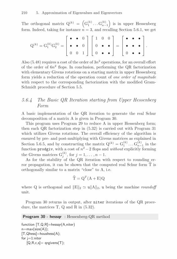
210 5. Approximation of Eigenvalues and Eigenvectors
The orthogonal matrix Q(k) =KG(k)
1 . . .G(k)n"1
Lis in upper Hessenberg
form. Indeed, taking for instance n = 3, and recalling Section 5.6.1, we get
Q(k) = G(k)1 G(k)
2 =
"
##$
• • 0
• • 0
0 0 1
%
&&'
"
##$
1 0 0
0 • •
0 • •
%
&&' =
"
##$
• • •
• • •
0 • •
%
&&' .
Also (5.48) requires a cost of the order of 3n2 operations, for an overall e!ortof the order of 6n2 flops. In conclusion, performing the QR factorizationwith elementary Givens rotations on a starting matrix in upper Hessenbergform yields a reduction of the operation count of one order of magnitudewith respect to the corresponding factorization with the modified Gram-Schmidt procedure of Section 5.5.
5.6.4 The Basic QR Iteration starting from Upper HessenbergForm
A basic implementation of the QR iteration to generate the real Schurdecomposition of a matrix A is given in Program 30.
This program uses Program 29 to reduce A in upper Hessenberg form;then each QR factorization step in (5.32) is carried out with Program 31which utilizes Givens rotations. The overall e"ciency of the algorithm isensured by pre- and post-multiplying with Givens matrices as explained inSection 5.6.5, and by constructing the matrix Q(k) = G(k)
1 . . .G(k)n"1 in the
function prodgiv, with a cost of n2"2 flops and without explicitly formingthe Givens matrices G(k)
j , for j = 1, . . . , n" 1.As for the stability of the QR iteration with respect to rounding er-
ror propagation, it can be shown that the computed real Schur form :T isorthogonally similar to a matrix “close” to A, i.e.
:T = QT (A + E)Q
where Q is orthogonal and +E+2 1 u+A+2, u being the machine roundo!unit.
Program 30 returns in output, after niter iterations of the QR proce-dure, the matrices T, Q and R in (5.32).
Program 30 - hessqr : Hessenberg-QR method
function [T,Q,R]=hessqr(A,niter)n=max(size(A));[T,Qhess]=houshess(A);for j=1:niter
[Q,R,c,s]= qrgivens(T);

5.6 The QR Method for Matrices in Hessenberg Form 211
T=R;for k=1:n-1,
T=gacol(T,c(k),s(k),1,k+1,k,k+1);end
end
Program 31 - givensqr : QR factorization with Givens rotations
function [Q,R,c,s]= qrgivens(H)[m,n]=size(H);for k=1:n-1
[c(k),s(k)]=givcos(H(k,k),H(k+1,k));H=garow(H,c(k),s(k),k,k+1,k,n);
endR=H; Q=prodgiv(c,s,n);
function Q=prodgiv(c,s,n)n1=n-1; n2=n-2;Q=eye(n); Q(n1,n1)=c(n1); Q(n,n)=c(n1);Q(n1,n)=s(n1); Q(n,n1)=-s(n1);for k=n2:-1:1,
k1=k+1; Q(k,k)=c(k); Q(k1,k)=-s(k);q=Q(k1,k1:n); Q(k,k1:n)=s(k)*q;Q(k1,k1:n)=c(k)*q;
end
Example 5.8 Consider the matrix A (already in Hessenberg form)
A =
"
########$
3 17 %37 18 %40
1 0 0 0 0
0 1 0 0 0
0 0 1 0 0
0 0 0 1 0
%
&&&&&&&&'
.
To compute its eigenvalues, given by %4, ±i, 2 and 5, we apply the QR methodand we compute the matrix T(40) after 40 iterations of Program 30. Notice thatthe algorithm converges to the real Schur decomposition of A (5.34), with threeblocks Rii of order 1 (i = 1, 2, 3) and with the block R44 = T(40)(4 : 5, 4 : 5)having eigenvalues equal to ±i
T(40) =
"
########$
4.9997 18.9739 %34.2570 32.8760 %28.4604
0 %3.9997 6.7693 %6.4968 5.6216
0 0 2 %1.4557 1.1562
0 0 0 0.3129 %0.8709
0 0 0 1.2607 %0.3129
%
&&&&&&&&'
.

212 5. Approximation of Eigenvalues and Eigenvectors
•
Example 5.9 Let us now employ the QR method to generate the Schur realdecomposition of the matrix A below, after reducing it to upper Hessenberg form
A =
"
########$
17 24 1 8 15
23 5 7 14 16
4 6 13 20 22
10 12 19 21 3
11 18 25 2 9
%
&&&&&&&&'
.
The eigenvalues of A are real and given (to four significant figures) by #1 =65, #2,3 = ±21.28 and #4,5 = ±13.13. After 40 iterations of Program 30, thecomputed matrix reads
T(40) =
"
########$
65 0 0 0 0
0 14.6701 14.2435 4.4848 %3.4375
0 16.6735 %14.6701 %1.2159 2.0416
0 0 0 %13.0293 %0.7643
0 0 0 %3.3173 13.0293
%
&&&&&&&&'
.
It is not upper triangular, but block upper triangular, with a diagonal blockR11 = 65 and the two blocks
R22 =
N14.6701 14.2435
16.6735 %14.6701
O
, R33 =
N%13.0293 %0.7643
%3.3173 13.0293
O
,
having spectrums given by '(R22) = #2,3 and '(R33) = #4,5 respectively.It is important to recognize that matrix T(40) is not the real Schur decomposi-
tion of A, but only a “cheating” version of it. In fact, in order for the QR methodto converge to the real Schur decomposition of A, it is mandatory to resort tothe shift techniques introduced in Section 5.7. •
5.6.5 Implementation of Transformation MatricesIn the definition (5.42) it is convenient to choose the minus sign, obtainingw(k) = x(n"k)"+x(n"k)+2e(n"k)
1 , in such a way that the vector Rn"kx(n"k)
is a positive multiple of e(n"k)1 . If xk+1 is positive, in order to avoid nu-
merical cancellations, the computation can be rationalized as follows
w(k)1 =
x2k+1 " +x(n"k)+22
xk+1 + +x(n"k)+2=
"n(
j=k+2
x2j
xk+1 + +x(n"k)+2.
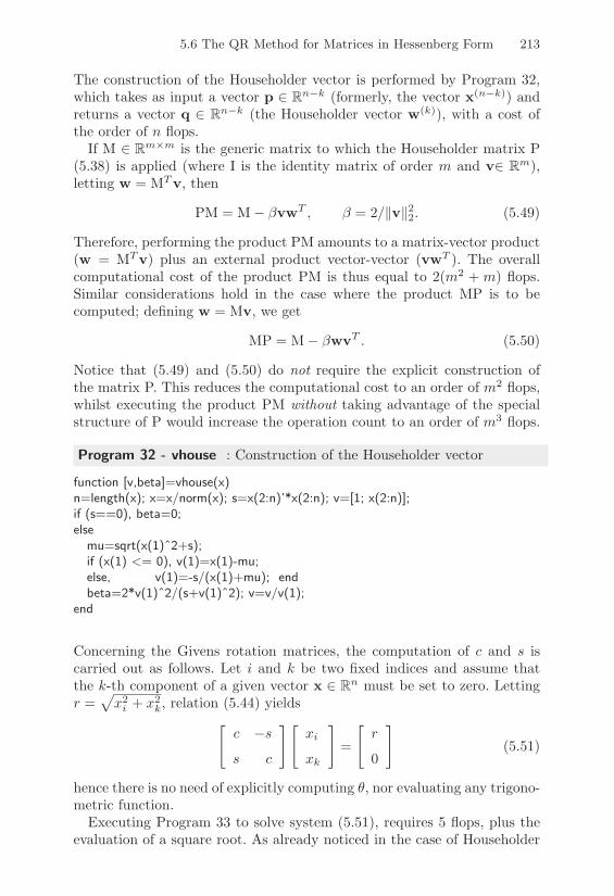
5.6 The QR Method for Matrices in Hessenberg Form 213
The construction of the Householder vector is performed by Program 32,which takes as input a vector p ! Rn"k (formerly, the vector x(n"k)) andreturns a vector q ! Rn"k (the Householder vector w(k)), with a cost ofthe order of n flops.
If M ! Rm!m is the generic matrix to which the Householder matrix P(5.38) is applied (where I is the identity matrix of order m and v! Rm),letting w = MTv, then
PM = M" #vwT , # = 2/+v+22. (5.49)
Therefore, performing the product PM amounts to a matrix-vector product(w = MTv) plus an external product vector-vector (vwT ). The overallcomputational cost of the product PM is thus equal to 2(m2 + m) flops.Similar considerations hold in the case where the product MP is to becomputed; defining w = Mv, we get
MP = M" #wvT . (5.50)
Notice that (5.49) and (5.50) do not require the explicit construction ofthe matrix P. This reduces the computational cost to an order of m2 flops,whilst executing the product PM without taking advantage of the specialstructure of P would increase the operation count to an order of m3 flops.
Program 32 - vhouse : Construction of the Householder vector
function [v,beta]=vhouse(x)n=length(x); x=x/norm(x); s=x(2:n)’*x(2:n); v=[1; x(2:n)];if (s==0), beta=0;else
mu=sqrt(x(1)ˆ2+s);if (x(1) <= 0), v(1)=x(1)-mu;else, v(1)=-s/(x(1)+mu); endbeta=2*v(1)ˆ2/(s+v(1)ˆ2); v=v/v(1);
end
Concerning the Givens rotation matrices, the computation of c and s iscarried out as follows. Let i and k be two fixed indices and assume thatthe k-th component of a given vector x ! Rn must be set to zero. Lettingr =
3x2i + x2
k, relation (5.44) yieldsN
c "s
s c
O Nxi
xk
O
=
Nr
0
O
(5.51)
hence there is no need of explicitly computing !, nor evaluating any trigono-metric function.
Executing Program 33 to solve system (5.51), requires 5 flops, plus theevaluation of a square root. As already noticed in the case of Householder

214 5. Approximation of Eigenvalues and Eigenvectors
matrices, even for Givens rotations we don’t have to explicitly compute thematrix G(i, k, !) to perform its product with a given matrix M! Rm!m.For that purpose Programs 34 and 35 are used, both at the cost of 6mflops. Looking at the structure (5.43) of matrix G(i, k, !), it is clear thatthe first algorithm only modifies rows i and k of M, whilst the second oneonly changes columns i and k of M.We conclude by noticing that the computation of the Householder vectorv and of the Givens sine and cosine (c, s), are well-conditioned operationswith respect to rounding errors (see [GL89], pp. 212-217 and the referencestherein).
The solution of system (5.51) is implemented in Program 33. The inputparameters are the vector components xi and xk, whilst the output dataare the Givens cosine and sine c and s.
Program 33 - givcos : Computation of Givens cosine and sine
function [c,s]=givcos(xi, xk)if (xk==0), c=1; s=0; else,
if abs(xk) > abs(xi)t=-xi/xk; s=1/sqrt(1+tˆ2); c=s*t;
elset=-xk/xi; c=1/sqrt(1+tˆ2); s=c*t;
endend
Programs 34 and 35 compute G(i, k, !)TM and MG(i, k, !) respectively.The input parameters c and s are the Givens cosine and sine. In Program34, the indices i and k identify the rows of the matrix M that are beinga!ected by the update M ; G(i, k, !)TM, while j1 and j2 are the indicesof the columns involved in the computation. Similarly, in Program 35 iand k identify the columns e!ected by the update M ; MG(i, k, !), whilej1 and j2 are the indices of the rows involved in the computation.
Program 34 - garow : Product G(i, k, !)TM
function [M]=garow(M,c,s,i,k,j1,j2)for j=j1:j2
t1=M(i,j);t2=M(k,j);M(i,j)=c*t1-s*t2;M(k,j)=s*t1+c*t2;
end
Program 35 - gacol : Product MG(i, k, !)
function [M]=gacol(M,c,s,j1,j2,i,k)for j=j1:j2
t1=M(j,i);
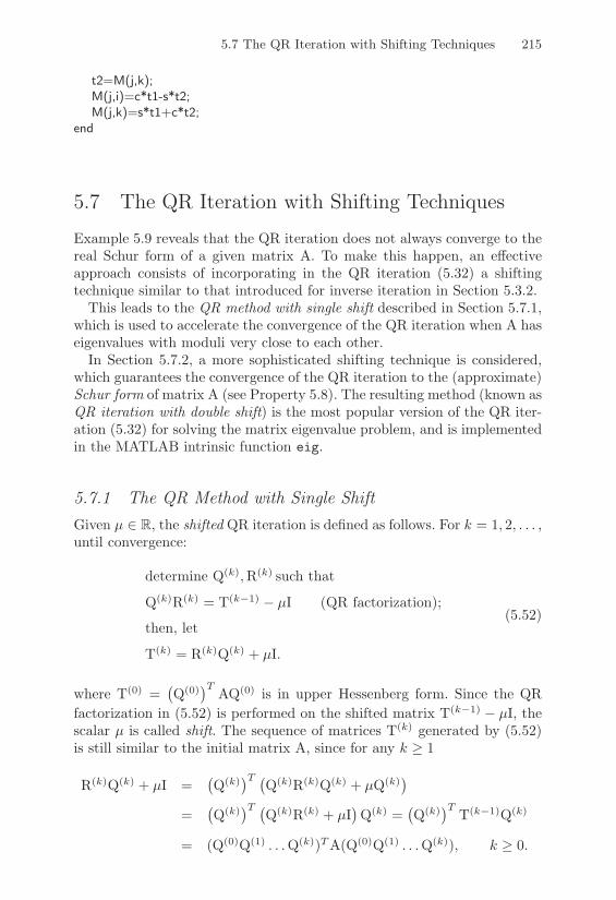
5.7 The QR Iteration with Shifting Techniques 215
t2=M(j,k);M(j,i)=c*t1-s*t2;M(j,k)=s*t1+c*t2;
end
5.7 The QR Iteration with Shifting Techniques
Example 5.9 reveals that the QR iteration does not always converge to thereal Schur form of a given matrix A. To make this happen, an e!ectiveapproach consists of incorporating in the QR iteration (5.32) a shiftingtechnique similar to that introduced for inverse iteration in Section 5.3.2.
This leads to the QR method with single shift described in Section 5.7.1,which is used to accelerate the convergence of the QR iteration when A haseigenvalues with moduli very close to each other.
In Section 5.7.2, a more sophisticated shifting technique is considered,which guarantees the convergence of the QR iteration to the (approximate)Schur form of matrix A (see Property 5.8). The resulting method (known asQR iteration with double shift) is the most popular version of the QR iter-ation (5.32) for solving the matrix eigenvalue problem, and is implementedin the MATLAB intrinsic function eig.
5.7.1 The QR Method with Single ShiftGiven µ ! R, the shifted QR iteration is defined as follows. For k = 1, 2, . . . ,until convergence:
determine Q(k),R(k) such that
Q(k)R(k) = T(k"1) " µI (QR factorization);
then, let
T(k) = R(k)Q(k) + µI.
(5.52)
where T(0) =8Q(0)9T AQ(0) is in upper Hessenberg form. Since the QR
factorization in (5.52) is performed on the shifted matrix T(k"1) " µI, thescalar µ is called shift. The sequence of matrices T(k) generated by (5.52)is still similar to the initial matrix A, since for any k ) 1
R(k)Q(k) + µI =8Q(k)9T 8
Q(k)R(k)Q(k) + µQ(k)9
=8Q(k)9T 8
Q(k)R(k) + µI9Q(k) =
8Q(k)9T T(k"1)Q(k)
= (Q(0)Q(1) . . .Q(k))TA(Q(0)Q(1) . . .Q(k)), k ) 0.

216 5. Approximation of Eigenvalues and Eigenvectors
Assume µ is fixed and that the eigenvalues of A are ordered in such a waythat
|$1 " µ| ) |$2 " µ| ) . . . ) |$n " µ|.Then it can be shown that, for 1 < j & n, the subdiagonal entry t(k)
j,j"1tends to zero with a rate that is proportional to the ratio
|($j " µ)/($j"1 " µ)|k.
This extends the convergence result (5.37) to the shifted QR method (see[GL89], Sections 7.5.2 and 7.3).
The result above suggests that if µ is chosen in such a way that
|$n " µ| < |$i " µ|, i = 1, . . . , n" 1,
then the matrix entry t(k)n,n"1 in the iteration (5.52) tends rapidly to zero
as k increases. (In the limit, if µ were equal to an eigenvalue of T(k), thatis of A, then t(k)
n,n"1 = 0 and t(k)n,n = µ). In practice one takes
µ = t(k)n,n, (5.53)
yielding the so called QR iteration with single shift. Correspondingly, theconvergence to zero of the sequence
Rt(k)n,n"1
Sis quadratic in the sense that
if |t(k)n,n"1|/+T(0)+2 = -k < 1, for some k ) 0, then |t(k+1)
n,n"1|/+T(0)+2 = O(-2k)
(see [Dem97], pp. 161-163 and [GL89], pp. 354-355).This can be profitably taken into account when programming the QR
iteration with single shift by monitoring the size of the subdiagonal entry|t(k)n,n"1|. In practice, t(k)
n,n"1 is set equal to zero if
|t(k)n,n"1| & +(|t(k)
n"1,n"1| + |t(k)n,n|), k ) 0, (5.54)
for a prescribed +, in general of the order of the roundo! unit. (This con-vergence test is adopted in the library EISPACK). If A is an Hessenbergmatrix, when for a certain k a(k)
n,n"1 is set to zero, t(k)n,n provides the desired
approximation of $n. Then the QR iteration with shift can continue on thematrix T(k)(1 : n " 1, 1 : n " 1), and so on. This is a deflation algorithm(for another example see Remark 5.3).
Example 5.10 We consider again the matrix A as in Example 5.9. Program 36,with toll equal to the roundo! unit, converges in 14 iterations to the followingapproximate real Schur form of A, which displays the correct eigenvalues of matrixA on its diagonal (to six significant figures)
T(40) =
"
########$
65 0 0 0 0
0 %21.2768 2.5888 %0.0445 %4.2959
0 0 %13.1263 %4.0294 %13.079
0 0 0 21.2768 %2.6197
0 0 0 0 13.1263
%
&&&&&&&&'
.

5.7 The QR Iteration with Shifting Techniques 217
We also report in Table 5.2 the convergence rate p(k) of the sequenceRt(k)n,n%1
S
(n = 5) computed as
p(k) = 1 +1
log(0k)log
|t(k)n,n%1|
|t(k%1)n,n%1|
, k ! 1.
The results show good agreement with the expected quadratic rate.
k |t(k)n,n"1|/+T(0)+2 p(k)
0 0.138651 1.5401 · 10"2 2.11222 1.2213 · 10"4 2.15913 1.8268 · 10"8 1.97754 8.9036 · 10"16 1.9449
TABLE 5.2. Convergence rate of the sequenceRt(k)n,n%1
Sin the QR iteration with
single shift
•
The coding of the QR iteration with single shift (5.52) is given in Pro-gram 36. The code utilizes Program 29 to reduce the matrix A in upperHessenberg form and Program 31 to perform the QR factorization step.The input parameters toll and itmax are the tolerance + in (5.54) andthe maximum admissible number of iterations, respectively. In output, theprogram returns the (approximate) real Schur form of A and the numberof iterations needed for its computation.
Program 36 - qrshift : QR iteration with single shift
function [T,iter]=qrshift(A,toll,itmax)n=max(size(A)); iter=0; [T,Q]=houshess(A);for k=n:-1:2I=eye(k);while abs(T(k,k-1)) > toll*(abs(T(k,k))+abs(T(k-1,k-1)))
iter=iter+1;if (iter > itmax),
returnendmu=T(k,k); [Q,R,c,s]=qrgivens(T(1:k,1:k)-mu*I);T(1:k,1:k)=R*Q+mu*I;
endT(k,k-1)=0;
end

218 5. Approximation of Eigenvalues and Eigenvectors
5.7.2 The QR Method with Double ShiftThe single-shift QR iteration (5.52) with the choice (5.53) for µ is e!ectiveif the eigenvalues of A are real, but not necessarily when complex conjugateeigenvalues are present, as happens in the following example.
Example 5.11 The matrix A / R4&4 (reported below to five significant figures)
A =
"
#####$
1.5726 %0.6392 3.7696 %1.3143
0.2166 %0.0420 0.4006 %1.2054
0.0226 0.3592 0.2045 %0.1411
%0.1814 1.1146 %3.2330 1.2648
%
&&&&&'
has eigenvalues {±i, 1, 2}, i being the imaginary unit. Running Program 36 withtoll equal to the roundo! unit yields after 100 iterations
T(101) =
"
#####$
2 1.1999 0.5148 4.9004
0 %0.0001 %0.8575 0.7182
0 1.1662 0.0001 %0.8186
0 0 0 1
%
&&&&&'.
The obtained matrix is the real Schur form of A, where the 212 block T(101)(2:3,2:3) has complex conjugate eigenvalues ±i. These eigenvalues cannot be computedby the algorithm (5.52)-(5.53) since µ is real. •
The problem with this example is that working with real matrices neces-sarily yields a real shift, whereas a complex one would be needed. The QRiteration with double shift is set up to account for complex eigenvalues andallows for removing the 2%2 diagonal blocks of the real Schur form of A.
Precisely, suppose that the QR iteration with single shift (5.52) detectsat some step k a 2%2 diagonal block R(k)
kk that cannot be reduced intoupper triangular form. Since the iteration is converging to the real Schurform of the matrix A the two eigenvalues of R(k)
kk are complex conjugateand will be denoted by $(k) and $(k). The double shift strategy consists of
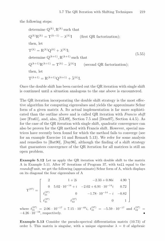
5.7 The QR Iteration with Shifting Techniques 219
the following steps:
determine Q(k),R(k) such that
Q(k)R(k) = T(k"1) " $(k)I (first QR factorization);
then, let
T(k) = R(k)Q(k) + $(k)I;
determine Q(k+1),R(k+1) such that
Q(k+1)R(k+1) = T(k) " $(k)I (second QR factorization);
then, let
T(k+1) = R(k+1)Q(k+1) + $(k)I.
(5.55)
Once the double shift has been carried out the QR iteration with single shiftis continued until a situation analogous to the one above is encountered.
The QR iteration incorporating the double shift strategy is the most e!ec-tive algorithm for computing eigenvalues and yields the approximate Schurform of a given matrix A. Its actual implementation is far more sophisti-cated than the outline above and is called QR iteration with Francis shift(see [Fra61], and, also, [GL89], Section 7.5 and [Dem97], Section 4.4.5). Asfor the case of the QR iteration with single shift, quadratic convergence canalso be proven for the QR method with Francis shift. However, special ma-trices have recently been found for which the method fails to converge (seefor an example Exercise 14 and Remark 5.13). We refer for some analysisand remedies to [Bat90], [Day96], although the finding of a shift strategythat guarantees convergence of the QR iteration for all matrices is still anopen problem.
Example 5.12 Let us apply the QR iteration with double shift to the matrixA in Example 5.11. After 97 iterations of Program 37, with toll equal to theroundo! unit, we get the following (approximate) Schur form of A, which displayson its diagonal the four eigenvalues of A
T(97) =
"
#####$
2 1 + 2i %2.33 + 0.86i 4.90
0 5.02 · 10%14 + i %2.02 + 6.91 · 10%14i 0.72
t(97)31 0 %1.78 · 10%14 % i %0.82
t(97)41 t(97)42 0 1
%
&&&&&'
where t(97)31 = 2.06 · 10%17 + 7.15 · 10%49i, t(97)41 = %5.59 · 10%17 and t(97)42 =%4.26 · 10%18, respectively. •
Example 5.13 Consider the pseudo-spectral di"erentiation matrix (10.73) oforder 5. This matrix is singular, with a unique eigenvalue # = 0 of algebraic

220 5. Approximation of Eigenvalues and Eigenvectors
multiplicity equal to 5 (see [CHQZ88], p. 44). In this case the QR method withdouble shift provides an inaccurate approximation of the spectrum of the ma-trix. Indeed, using Program 37, with toll=eps, the method converges after 59iterations to an upper triangular matrix with diagonal entries given by 0.0020,0.0006± 0.0019i and %0.0017± 0.0012i, respectively. Using the MATLAB intrin-sic function eig yields instead the eigenvalues %0.0024, %0.0007 ± 0.0023i and0.0019 ± 0.0014i. •
A basic implementation of the QR iteration with double shift is providedin Program 37. The input/output parameters are the same as those ofProgram 36. The output matrix T is the approximate Schur form of matrixA.
Program 37 - qr2shift : QR iteration with double shift
function [T,iter]=qr2shift(A,toll,itmax)n=max(size(A)); iter=0; [T,Q]=houshess(A);for k=n:-1:2I=eye(k);while abs(T(k,k-1)) > toll*(abs(T(k,k))+abs(T(k-1,k-1)))
iter=iter+1; if (iter > itmax), return, endmu=T(k,k); [Q,R,c,s]=qrgivens(T(1:k,1:k)-mu*I);T(1:k,1:k)=R*Q+mu*I;if (k > 2),
Tdiag2=abs(T(k-1,k-1))+abs(T(k-2,k-2));if abs(T(k-1,k-2)) ¡= toll*Tdiag2;
[lambda]=eig(T(k-1:k,k-1:k));[Q,R,c,s]=qrgivens(T(1:k,1:k)-lambda(1)*I);T(1:k,1:k)=R*Q+lambda(1)*I;[Q,R,c,s]=qrgivens(T(1:k,1:k)-lambda(2)*I);T(1:k,1:k)=R*Q+lambda(2)*I;
endend
end, T(k,k-1)=0;endI=eye(2);while (abs(T(2,1)) > toll*(abs(T(2,2))+abs(T(1,1)))) & (iter <= itmax)
iter=iter+1; mu=T(2,2);[Q,R,c,s]=qrgivens(T(1:2,1:2)-mu*I); T(1:2,1:2)=R*Q+mu*I;
end

5.8 Computing the Eigenvectors and the SVD of a Matrix 221
5.8 Computing the Eigenvectors and the SVD of aMatrix
The power and inverse iterations described in Section 5.3.2 can be usedto compute a selected number of eigenvalue/eigenvector pairs. If all theeigenvalues and eigenvectors of a matrix are needed, the QR iteration can beprofitably employed to compute the eigenvectors as shown in Sections 5.8.1and 5.8.2. In Section 5.8.3 we deal with the computation of the singularvalue decomposition (SVD) of a given matrix.
5.8.1 The Hessenberg Inverse IterationFor any approximate eigenvalue $ computed by the QR iteration as de-scribed in Section 5.7.2, the inverse iteration (5.28) can be applied to thematrix H = QTAQ in Hessenberg form, yielding an approximate eigenvec-tor q. Then, the eigenvector x associated with $ is computed as x = Qq.Clearly, one can take advantage of the structure of the Hessenberg matrixfor an e"cient solution of the linear system at each step of (5.28). Typi-cally, only one iteration is required to produce an adequate approximationof the desired eigenvector x (see [GL89], Section 7.6.1 and [PW79] for moredetails).
5.8.2 Computing the Eigenvectors from the Schur Form of aMatrix
Suppose that the (approximate) Schur form QHAQ=T of a given matrixA! Rn!n has been computed by the QR iteration with double shift, Qbeing a unitary matrix and T being upper triangular.
Then, if Ax=$x, we have QHAQQHx= QH $x, i.e., letting y=QHx, Ty=$y holds. Therefore y is an eigenvector of T, so that to compute theeigenvectors of A we can work directly on the Schur form T.
Assume for simplicity that $ = tkk ! C is a simple eigenvalue of A. Thenthe upper triangular matrix T can be decomposed as
T =
"
##$
T11 v T13
0 $ wT
0 0 T33
%
&&' ,
where T11 ! C(k"1)!(k"1) and T33 ! C(n"k)!(n"k) are upper triangularmatrices, v! Ck"1, w! Cn"k and $ '! ((T11) 2 ((T33).

222 5. Approximation of Eigenvalues and Eigenvectors
Thus, letting y =8yTk"1, y,y
Tn"k
9, with yk"1 ! Ck"1, y ! C and yn"k !
Cn"k, the matrix eigenvector problem (T - $I) y=0 can be written as)**+
**,
(T11 " $Ik"1)yk"1+ vy+ T13yn"k = 0
wTyn"k = 0
(T33 " $In"k)yn"k = 0.
(5.56)
Since $ is simple, both matrices T11 " $Ik"1 and T33 " $In"k are nonsin-gular, so that the third equation in (5.56) yields yn"k = 0 and the firstequation becomes
(T11 " $Ik"1)yk"1 = "vy.
Setting arbitrarily y = 1 and solving the triangular system above for yk"1yields (formally)
y =
G
\\H
"(T11 " $Ik"1)"1v
1
0
I
]]J .
The desired eigenvector x can then be computed as x=Qy.An e"cient implementation of the above procedure is carried out in the
intrinsic MATLAB function eig. Invoking this function with the format [V,D]= eig(A) yields the matrix V whose columns are the right eigenvectorsof A and the diagonal matrix D contains its eigenvalues. Further details canbe found in the strvec subroutine in the LAPACK library, while for thecomputation of eigenvectors in the case where A is symmetric, we refer to[GL89], Chapter 8 and [Dem97], Section 5.3.
5.8.3 Approximate Computation of the SVD of a MatrixIn this section we describe the Golub-Kahan-Reinsch algorithm for thecomputation of the SVD of a matrix A ! Rm!n with m ) n (see [GL89],Section 5.4). The method consists of two phases, a direct one and an iter-ative one.
In the first phase A is transformed into an upper trapezoidal matrix ofthe form
UTAV =4
B0
5, (5.57)
where U and V are two orthogonal matrices and B ! Rn!n is upper bidi-agonal. The matrices U and V are generated using n + m" 3 Householdermatrices U1, . . . ,Um"1,V1, . . . ,Vn"2 as follows.

5.8 Computing the Eigenvectors and the SVD of a Matrix 223
The algorithm initially generates U1 in such a way that the matrix A(1) =U1A has a(1)
i1 = 0 if i > 1. Then, V1 is determined so that A(2) = A(1)V1
has a(2)1j = 0 for j > 2, preserving at the same time the null entries of the
previous step. The procedure is repeated starting from A(2), and taking U2
such that A(3) = U2A(2) has a(3)i2 = 0 for i > 2 and V2 in such a way that
A(4) = A(3)V2 has a(4)2j = 0 for j > 3, yet preserving the null entries already
generated. For example, in the case m = 5, n = 4 the first two steps of thereduction process yield
A(1) = U1A =
"
#######$
• • • •
0 • • •
0 • • •
0 • • •
0 • • •
%
&&&&&&&'
"( A(2) = A(1)V1 =
"
#######$
• • 0 0
0 • • •
0 • • •
0 • • •
0 • • •
%
&&&&&&&'
,
having denoted by • the entries of the matrices that in principle are di!erentthan zero. After at most m" 1 steps, we find (5.57) with
U = U1U2 . . .Um"1, V = V1V2 . . .Vn"2.
In the second phase, the obtained matrix B is reduced into a diagonalmatrix & using the QR iteration. Precisely, a sequence of upper bidiagonalmatrices B(k) are constructed such that, as k ( ,, their o!-diagonalentries tend to zero quadratically and the diagonal entries tend to thesingular values (i of A. In the limit, the process generates two orthogonalmatrices W and Z such that
WTBZ = & = diag((1, . . . ,(n).
The SVD of A is then given by
UTAV =4&0
5,
with U = Udiag(W, Im"n) and V = VZ.The computational cost of this procedure is 2m2n + 4mn2 + 9
2n3 flops,
which reduces to 2mn2" 23n
3 flops if only the singular values are computed.In this case, recalling what was stated in Section 3.13 about ATA, themethod described in the present section is preferable to computing directlythe eigenvalues of ATA and then taking their square roots.
As for the stability of this procedure, it can be shown that the computed(i turn out to be the singular values of the matrix A + %A with
+%A+2 & Cmnu+A+2,

224 5. Approximation of Eigenvalues and Eigenvectors
Cmn being a constant dependent on n, m and the roundo! unit u. For otherapproaches to the computation of the SVD of a matrix, see [Dat95] and[GL89].
5.9 The Generalized Eigenvalue Problem
Let A,B ! Cn!n be two given matrices; for any z ! C, we call A " zB amatrix pencil and denote it by (A,B). The set ((A,B) of the eigenvalues of(A,B) is defined as
((A,B) = {µ ! C : det(A" µB) = 0} .
The generalized matrix eigenvalue problem can be formulated as: find $ !((A,B) and a nonnull vector x ! Cn such that
Ax = $Bx. (5.58)
The pair ($,x) satisfying (5.58) is an eigenvalue/eigenvector pair of thepencil (A,B). Note that by setting B=In in (5.58) we recover the standardmatrix eigenvalue problem considered thus far.
Problems like (5.58) arise frequently in engineering applications, e.g.,in the study of vibrations of structures (buildings, aircrafts and bridges)or in the mode analysis for waveguides (see [Inm94] and [Bos93]). Anotherexample is the computation of the extremal eigenvalues of a preconditionedmatrix P"1A (in which case B = P in (5.58)) when solving a linear systemwith an iterative method (see Remark 4.2).
Let us introduce some definitions. We say that the pencil (A,B) is regularif det(A-zB) is not identically zero, otherwise the pencil is singular. When(A,B) is regular, p(z) = det(A" zB) is the characteristic polynomial of thepencil; denoting by k the degree of p, the eigenvalues of (A,B) are definedas:
1. the roots of p(z) = 0, if k = n;
2. , if k < n (with multiplicity equal to n" k).
Example 5.14 (Taken from [Par80], [Saa92] and [GL89])
A =-%1 0
0 1
., B =
-0 11 0
.p(z) = z2 + 1 =* '(A,B) = ±i
A =-%1 0
0 0
., B =
-0 00 1
.p(z) = z =* '(A,B) = {0, #}
A =-
1 20 0
., B =
-1 00 0
.p(z) = 0 =* '(A,B) = C.
The first pair of matrices shows that symmetric pencils, unlike symmetric ma-trices, may exhibit complex conjugate eigenvalues. The second pair is a regularpencil displaying an eigenvalue equal to infinity, while the third pair is an exampleof singular pencil. •

5.9 The Generalized Eigenvalue Problem 225
5.9.1 Computing the Generalized Real Schur FormThe definitions and examples above imply that the pencil (A,B) has n finiteeigenvalues i! B is nonsingular.
In such a case, a possible approach to the solution of problem (5.58) isto transform it into the equivalent eigenvalue problem Cx = $x, where thematrix C is the solution of the system BC = A, then apply the QR iterationto C. For actually computing the matrix C, one can use Gauss eliminationwith pivoting or the techniques shown in Section 3.6. This procedure canyield inaccurate results if B is ill-conditioned, since computing C is a!ectedby rounding errors of the order of u +A+2+B"1+2 (see [GL89], p. 376).
A more attractive approach is based on the following result, which gen-eralizes the Schur decomposition theorem 1.5 to the case of regular pencilsto (for a proof, see [Dat95], p. 497).
Property 5.10 (Generalized Schur decomposition) Let (A,B) be aregular pencil. Then, there exist two unitary matrices U and Z such thatUHAZ = T, UHBZ = S, where T and S are upper triangular. For i =1, . . . , n the eigenvalues of (A,B) are given by
$i = tii/sii, if sii '= 0,
$i = ,, if tii '= 0, sii = 0.
Exactly as in the matrix eigenvalue problem, the generalized Schur formcannot be explicitly computed, so the counterpart of the real Schur form(5.34) has to be computed. Assuming that the matrices A and B are real, itcan be shown that there exist two orthogonal matrices U and Z such thatT = UTAZ is upper quasi-triangular and S = UTBZ is upper triangular.This decomposition is known as the generalized real Schur decompositionof a pair (A,B) and can be computed by a suitably modified version of theQR algorithm, known as QZ iteration, which consists of the following steps(for a more detailed description, see [GL89], Section 7.7, [Dat95], Section9.3):
1. reduce A and B into upper Hessenberg form and upper triangularform, respectively, i.e., find two orthogonal matrices Q and Z suchthat A = QTAZ is upper Hessenberg and B = QTBZ is upper trian-gular;
2. the QR iteration is applied to the matrix AB"1 to reduce it to realSchur form.
To save computational resources, the QZ algorithm overwrites the matricesA and B on their upper Hessenberg and triangular forms and requires 30n3
flops; an additional cost of 36n3 operations is required if Q and Z are

226 5. Approximation of Eigenvalues and Eigenvectors
also needed. The method is implemented in the LAPACK library in thesubroutine sgges and can be invoked in the MATLAB environment withthe command eig(A,B).
5.9.2 Generalized Real Schur Form of Symmetric-DefinitePencils
A remarkable situation occurs when both A and B are symmetric, and oneof them, say B, is also positive definite. In such a case, the pair (A,B) formsa symmetric-definite pencil for which the following result holds.
Theorem 5.7 The symmetric-definite pencil (A,B) has real eigenvaluesand linearly independent eigenvectors. Moreover, the matrices A and B canbe simultaneously diagonalized. Precisely, there exists a nonsingular matrixX ! Rn!n such that
XTAX = % = diag($1,$2, . . . ,$n), XTBX = In,
where for i = 1, . . . , n, $i are the eigenvalues of the pencil (A,B).
Proof. Since B is symmetric positive definite, it admits a unique Cholesky fac-torization B = HTH, where H is upper triangular (see Section 3.4.2). From (5.58)we deduce that Cz = #z with C = H%TAH%1, z = Hx, where (#,x) is aneigenvalue/eigenvector pair of (A,B).
The matrix C is symmetric; therefore, its eigenvalues are real and a set oforthonormal eigenvectors (y1, . . . ,yn) = Y exists. As a consequence, letting X =H%1Y allows for simultaneously diagonalizing both A and B since
XTAX = YTH%TAH%1Y = YTCY = & = diag(#1, . . . ,#n),
XTBX = YTH%TBH%1Y = YTY = In.
!
The following QR-Cholesky algorithm computes the eigenvalues $i andthe corresponding eigenvectors xi of a symmetric-definite pencil (A,B), fori = 1, . . . , n (see for more details [GL89], Section 8.7, [Dat95], Section 9.5):
1. compute the Cholesky factorization B = HTH;
2. compute C = H"TAH"1;
3. for i = 1, . . . , n, compute the eigenvalues $i and eigenvectors zi of thesymmetric matrix C using the QR iteration. Then construct from theset {zi} an orthonormal set of eigenvectors {yi} (using, for instance,the modified Gram-Schmidt procedure of Section 3.4.3);
4. for i = 1, . . . , n, compute the eigenvectors xi of the pencil (A,B) bysolving the systems Hxi = yi.
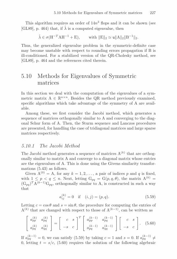
5.10 Methods for Eigenvalues of Symmetric matrices 227
This algorithm requires an order of 14n3 flops and it can be shown (see[GL89], p. 464) that, if $ is a computed eigenvalue, then
$ ! ((H"TAH"1 + E), with +E+2 1 u+A+2+B"1+2.
Thus, the generalized eigenvalue problem in the symmetric-definite casemay become unstable with respect to rounding errors propagation if B isill-conditioned. For a stabilized version of the QR-Cholesky method, see[GL89], p. 464 and the references cited therein.
5.10 Methods for Eigenvalues of Symmetricmatrices
In this section we deal with the computation of the eigenvalues of a sym-metric matrix A ! Rn!n. Besides the QR method previously examined,specific algorithms which take advantage of the symmetry of A are avail-able.
Among these, we first consider the Jacobi method, which generates asequence of matrices orthogonally similar to A and converging to the diag-onal Schur form of A. Then, the Sturm sequence and Lanczos proceduresare presented, for handling the case of tridiagonal matrices and large sparsematrices respectively.
5.10.1 The Jacobi MethodThe Jacobi method generates a sequence of matrices A(k) that are orthog-onally similar to matrix A and converge to a diagonal matrix whose entriesare the eigenvalues of A. This is done using the Givens similarity transfor-mations (5.43) as follows.
Given A(0) = A, for any k = 1, 2, . . . , a pair of indices p and q is fixed,with 1 & p < q & n. Next, letting Gpq = G(p, q, !), the matrix A(k) =(Gpq)TA(k"1)Gpq, orthogonally similar to A, is constructed in such a waythat
a(k)ij = 0 if (i, j) = (p, q). (5.59)
Letting c = cos ! and s = sin !, the procedure for computing the entries ofA(k) that are changed with respect to those of A(k"1), can be written as
"
$a(k)pp a(k)
pq
a(k)pq a(k)
%
' =
Nc s
"s c
OT"
$a(k"1)pp a(k"1)
pq
a(k"1)pq a(k"1)
%
'N
c s
"s c
O
. (5.60)
If a(k"1)pq = 0, we can satisfy (5.59) by taking c = 1 and s = 0. If a(k"1)
pq '=0, letting t = s/c, (5.60) requires the solution of the following algebraic

228 5. Approximation of Eigenvalues and Eigenvectors
equation
t2 + 2-t" 1 = 0, - =a(k"1)qq " a(k"1)
pp
2a(k"1)pq
. (5.61)
The root t = 1/(- +3
1 + -2) is chosen in (5.61) if - ) 0, otherwise wetake t = "1/("- +
31 + -2); next, we let
c =1/
1 + t2, s = ct. (5.62)
To examine the rate at which the o!-diagonal entries of A(k) tend to zero,it is convenient to introduce, for any matrix M ! Rn!n, the nonnegativequantity
)(M) =
G
\Hn(
i,j=1i '=j
m2ij
I
]J
1/2
=
6
+M+2F "n(
i=1
m2ii
71/2
. (5.63)
The Jacobi method ensures that )(A(k)) & )(A(k"1)) for any k ) 1.Indeed, the computation of (5.63) for matrix A(k) yields
()(A(k)))2 = ()(A(k"1)))2 " 2Ka(k"1)pq
L2& ()(A(k"1)))2. (5.64)
The estimate (5.64) suggests that, at each step k, the optimal choice of theindices p and q is that corresponding to the entry in A(k"1) such that
|a(k"1)pq | = max
i '=j|a(k"1)
ij |.
The computational cost of this strategy is of the order of n2 flops for thesearch of the maximum module entry, while the updating step A(k) =(Gpq)TA(k"1)Gpq requires only a cost of the order of n flops, as alreadynoticed in Section 5.6.5. It is thus convenient to resort to the so called rowcyclic Jacobi method, in which the choice of the indices p and q is done bya row-sweeping of the matrix A(k) according to the following algorithm: forany k = 1, 2, . . . and for any i-th row of A(k) (i = 1, . . . , n " 1), we setp = i and q = (i+1), . . . , n. Each complete sweep requires N = n(n"1)/2Jacobi transformations. Assuming that |$i " $j | ) % for i '= j, it can beshown that the cyclic Jacobi method converges quadratically, that is (see[Wil65], [Wil62])
)(A(k+N)) & 1%/
2()(A(k)))2, k = 1, 2, . . .
For further details of the algorithm, we refer to [GL89], Section 8.4.

5.10 Methods for Eigenvalues of Symmetric matrices 229
Example 5.15 Let us apply the cyclic Jacobi method to the Hilbert matrix H4,whose eigenvalues read (to five significant figures) #1 = 1.5002, #2 = 1.6914·10%1,#3 = 6.7383 · 10%3 and #4 = 9.6702 · 10%5. Running Program 40 with toll =10%15, the method converges in 3 sweeps to a matrix whose diagonal entriescoincide with the eigenvalues of H4 unless 4.4409 · 10%16. As for the o"-diagonalentries, the values attained by '(H(k)
4 ) are reported in Table 5.3. •
Sweep )(H(k)4 ) Sweep )(H(k)
4 ) Sweep )(H(k)4 )
1 5.262 · 10"2 2 3.824 · 10"5 3 5.313 · 10"16
TABLE 5.3. Convergence of the cyclic Jacobi algorithm
Formulae (5.63) and (5.62) are implemented in Programs 38 and 39.
Program 38 - psinorm : Evaluation of )(A)
function [psi]=psinorm(A)n=max(size(A)); psi=0;for i=1:(n-1), for j=(i+1):n, psi=psi+A(i,j)ˆ2+A(j,i)ˆ2; end; end; psi=sqrt(psi);
Program 39 - symschur : Evaluation of c and s
function [c,s]=symschur(A,p,q)if (A(p,q)==0), c=1; s=0; else,eta=(A(q,q)-A(p,p))/(2*A(p,q));if (eta >= 0), t=1/(eta+sqrt(1+etaˆ2));else, t=-1/(-eta+sqrt(1+etaˆ2)); end; c=1/sqrt(1+tˆ2); s=c*t;end
A coding of the cyclic Jacobi method is implemented in Program 40.This program gets as input parameters the symmetric matrix A ! Rn!n
and a tolerance toll. The program returns a matrix D = GTAG, G be-ing orthogonal, such that )(D) & toll+A+F , the value of )(D) and thenumber of sweeps to achieve convergence.
Program 40 - cycjacobi : Cyclic Jacobi method for symmetric matrices
function [D,sweep,psi]=cycjacobi(A,toll)n=max(size(A)); D=A; psiD=norm(A,’fro’);epsi=toll*psiD; psiD=psinorm(D); [psi]=psiD; sweep=0;while (psiD > epsi), sweep=sweep+1;for p=1:(n-1), for q=(p+1):n[c,s]=symschur(D,p,q); [D]=gacol(D,c,s,1,n,p,q); [D]=garow(D,c,s,p,q,1,n);end; end; psiD=psinorm(D); psi=[psi; psiD];end

230 5. Approximation of Eigenvalues and Eigenvectors
5.10.2 The Method of Sturm SequencesIn this section we deal with the calculation of the eigenvalues of a real,tridiagonal and symmetric matrix T. Typical instances of such a problemarise when applying the Householder transformation to a given symmetricmatrix A (see Section 5.6.2) or when solving boundary value problems inone spatial dimension (see for an example Section 5.12.1).
We analyze the method of Sturm sequences, or Givens method, introducedin [Giv54]. For i = 1, . . . , n, we denote by di the diagonal entries of T and bybi, i = 1, . . . , n"1, the elements of the upper and lower subdiagonals of T.We shall assume that bi '= 0 for any i. Otherwise, indeed, the computationreduces to problems of less complexity.
Letting Ti be the principal minor of order i of matrix T and p0(x) = 1,we define for i = 1, . . . , n the following sequence of polynomials pi(x) =det(Ti " xIi)
p1(x) = d1 " x
pi(x) = (di " x)pi"1(x)" b2i"1pi"2(x), i = 2, . . . , n.(5.65)
It can be checked that pn is the characteristic polynomial of T; the com-putational cost of its evaluation at point x is of the order of 2n flops. Thesequence (5.65) is called the Sturm sequence owing to the following result,for whose proof we refer to [Wil65], Chapter 2, Section 47 and Chapter 5,Section 37.
Property 5.11 (of Sturm sequence) For i = 2, . . . , n the eigenvaluesof Ti"1 strictly separate those of Ti, that is
$i(Ti) < $i"1(Ti"1) < $i"1(Ti) < . . . < $2(Ti) < $1(Ti"1) < $1(Ti).
Moreover, letting for any real number µ
Sµ = {p0(µ), p1(µ), . . . , pn(µ)},
the number s(µ) of sign changes in Sµ yields the number of eigenvalues of Tthat are strictly less than µ, with the convention that pi(µ) has opposite signto pi"1(µ) if pi(µ) = 0 (two consecutive elements in the sequence cannotvanish at the same value of µ).
Example 5.16 Let T be the tridiagonal part of the Hilbert matrix H4 / R4&4,having entries hij = 1/(i + j % 1). The eigenvalues of T are (to five significantfigures) #1 = 1.2813, #2 = 0.4205, #3 = %0.1417 and #4 = 0.1161. Taking µ = 0,Program 41 computes the following Sturm sequence
S0 = {p0(0), p1(0), p2(0), p3(0), p4(0)} = {1, 1, 0.0833,%0.0458,%0.0089}
from which, applying Property 5.11, one concludes that matrix T has one eigen-value less than 0. In the case of matrix T = tridiag4(%1, 2,%1), with eigenvalues
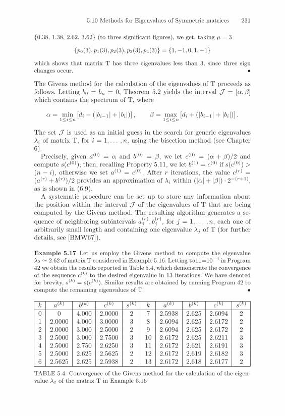
5.10 Methods for Eigenvalues of Symmetric matrices 231
{0.38, 1.38, 2.62, 3.62} (to three significant figures), we get, taking µ = 3
{p0(3), p1(3), p2(3), p3(3), p4(3)} = {1,%1, 0, 1,%1}
which shows that matrix T has three eigenvalues less than 3, since three signchanges occur. •
The Givens method for the calculation of the eigenvalues of T proceeds asfollows. Letting b0 = bn = 0, Theorem 5.2 yields the interval J = [",#]which contains the spectrum of T, where
" = min1%i%n
[di " (|bi"1| + |bi|)] , # = max1%i%n
[di + (|bi"1| + |bi|)] .
The set J is used as an initial guess in the search for generic eigenvalues$i of matrix T, for i = 1, . . . , n, using the bisection method (see Chapter6).
Precisely, given a(0) = " and b(0) = #, we let c(0) = (" + #)/2 andcompute s(c(0)); then, recalling Property 5.11, we let b(1) = c(0) if s(c(0)) >(n " i), otherwise we set a(1) = c(0). After r iterations, the value c(r) =(a(r) + b(r))/2 provides an approximation of $i within (|"| + |#|) · 2"(r+1),as is shown in (6.9).
A systematic procedure can be set up to store any information aboutthe position within the interval J of the eigenvalues of T that are beingcomputed by the Givens method. The resulting algorithm generates a se-quence of neighboring subintervals a(r)
j , b(r)j , for j = 1, . . . , n, each one ofarbitrarily small length and containing one eigenvalue $j of T (for furtherdetails, see [BMW67]).
Example 5.17 Let us employ the Givens method to compute the eigenvalue#2 0 2.62 of matrix T considered in Example 5.16. Letting toll=10%4 in Program42 we obtain the results reported in Table 5.4, which demonstrate the convergenceof the sequence c(k) to the desired eigenvalue in 13 iterations. We have denotedfor brevity, s(k) = s(c(k)). Similar results are obtained by running Program 42 tocompute the remaining eigenvalues of T. •
k a(k) b(k) c(k) s(k) k a(k) b(k) c(k) s(k)
0 0 4.000 2.0000 2 7 2.5938 2.625 2.6094 21 2.0000 4.000 3.0000 3 8 2.6094 2.625 2.6172 22 2.0000 3.000 2.5000 2 9 2.6094 2.625 2.6172 23 2.5000 3.000 2.7500 3 10 2.6172 2.625 2.6211 34 2.5000 2.750 2.6250 3 11 2.6172 2.621 2.6191 35 2.5000 2.625 2.5625 2 12 2.6172 2.619 2.6182 36 2.5625 2.625 2.5938 2 13 2.6172 2.618 2.6177 2
TABLE 5.4. Convergence of the Givens method for the calculation of the eigen-value #2 of the matrix T in Example 5.16

232 5. Approximation of Eigenvalues and Eigenvectors
An implementation of the polynomial evaluation (5.65) is given in Pro-gram 41. This program receives in input the vectors dd and bb containingthe main and the upper diagonals of T. The output values pi(x) are stored,for i = 0, . . . , n, in the vector p.
Program 41 - sturm : Sturm sequence evaluation
function [p]=sturm(dd,bb,x)n=length(dd); p(1)=1; p(2)=d(1)-x;for i=2:n, p(i+1)=(dd(i)-x)*p(i)-bb(i-1)ˆ2*p(i-1); end
A basic implementation of the Givens method is provided in Program42. In input, ind is the pointer to the searched eigenvalue, while the otherparameters are similar to those in Program 41. In output the values ofthe elements of sequences a(k), b(k) and c(k) are returned, together withthe required number of iterations niter and the sequence of sign changess(c(k)).
Program 42 - givsturm : Givens method using the Sturm sequence
function [ak,bk,ck,nch,niter]=givsturm(dd,bb,ind,toll)[a, b]=bound(dd,bb); dist=abs(b-a); s=abs(b)+abs(a);n=length(d); niter=0; nch=[];while (dist > (toll*s)),
niter=niter+1; c=(b+a)/2;ak(niter)=a; bk(niter)=b; ck(niter)=c;nch(niter)=chcksign(dd,bb,c);if (nch(niter) > (n-ind)), b=c;else, a=c; end; dist=abs(b-a); s=abs(b)+abs(a);
end
Program 43 - chcksign : Sign changes in the Sturm sequence
function nch=chcksign(dd,bb,x)[p]=sturm(dd,bb,x); n=length(dd); nch=0; s=0;for i=2:(n+1),
if ((p(i)*p(i-1)) <= 0), nch=nch+1; endif (p(i)==0), s=s+1; end
endnch=nch-s;
Program 44 - bound : Calculation of the interval J = [",#]
function [alfa,beta]=bound(dd,bb)n=length(dd); alfa=dd(1)-abs(bb(1)); temp=dd(n)-abs(bb(n-1));if (temp < alfa), alfa=temp; end;for i=2:(n-1),
temp=dd(i)-abs(bb(i-1))-abs(bb(i));

5.11 The Lanczos Method 233
if (temp < alfa), alfa=temp; end;endbeta=dd(1)+abs(bb(1)); temp=dd(n)+abs(bb(n-1));if (temp > beta), beta=temp; end;for i=2:(n-1),
temp=dd(i)+abs(bb(i-1))+abs(bb(i));if (temp > beta), beta=temp; end;
end
5.11 The Lanczos Method
Let A ! Rn!n be a symmetric sparse matrix, whose (real) eigenvalues areordered as
$1 ) $2 ) . . . ) $n"1 ) $n. (5.66)
When n is very large, the Lanczos method [Lan50] described in Section4.4.3 can be applied to approximate the extremal eigenvalues $n and $1. Itgenerates a sequence of tridiagonal matrices Hm whose extremal eigenvaluesrapidly converge to the extremal eigenvalues of A.
To estimate the convergence of the tridiagonalization process, we intro-duce the Rayleigh quotient r(x) = (xTAx)/(xTx) associated with a nonnullvector x ! Rn. The following result, known as Courant-Fisher Theorem,holds (for the proof see [GL89], p. 394)
$1(A) = maxx#Rn
x'=0
r(x), $n(A) = minx#Rn
x'=0
r(x).
Its application to the matrix Hm = VTmAVm, yields
$1(Hm) = maxx#Rn
x'=0
(Vmx)TA(Vmx)xTx
= max$x$2=1
r(Hmx) & $1(A)
$m(Hm) = minx#Rn
x'=0
(Vmx)TA(Vmx)xTx
= min$x$2=1
r(Hmx) ) $n(A).(5.67)
At each step of the Lanczos method, the estimates (5.67) provide a lowerand upper bound for the extremal eigenvalues of A. The convergence of thesequences {$1(Hm)} and {$m(Hm)} to $1 and $n, respectively, is governedby the following property, for whose proof we refer to [GL89], pp. 475-477.
Property 5.12 Let A ! Rn!n be a symmetric matrix with eigenvaluesordered as in (5.66) and let u1, . . . ,un be the corresponding orthonormaleigenvectors. If -1, . . . , -m denote the eigenvalues of Hm, with -1 ) -2 ). . . ) -m, then
$1 ) -1 ) $1 "($1 " $n)(tan41)2
(Tm"1(1 + 2)1))2,

234 5. Approximation of Eigenvalues and Eigenvectors
where cos41 = |(q(1))Tu1|, )1 = ($1 " $2)/($2 " $n) and Tm"1(x) is theChebyshev polynomial of degree m" 1 (see Section 10.1.1).
A similar result holds of course for the convergence estimate of the eigen-values -m to $n
$n & -m & $n +($1 " $n)(tan4n)2
(Tm"1(1 + 2)n))2,
where )n = ($n"1 " $n)/($1 " $n"1) and cos4n = |(q(n))Tun|.
A naive implementation of the Lanczos algorithm can be a!ected by nu-merical instability due to propagation of rounding errors. In particular, theLanczos vectors will not verify the mutual orthogonality relation, makingthe extremal properties (5.67) false. This requires careful programming ofthe Lanczos iteration by incorporating suitable reorthogonalization proce-dures as described in [GL89], Sections 9.2.3-9.2.4.
Despite this limitation, the Lanczos method has two relevant features:it preserves the sparsity pattern of the matrix (unlike Householder tridiag-onalization), and such a property makes it quite attractive when dealingwith large size matrices; furthermore, it converges to the extremal eigen-values of A much more rapidly than the power method does (see [Kan66],[GL89], p. 477).
The Lanczos method can be generalized to compute the extremal eigen-values of an unsymmetric matrix along the same lines as in Section 4.5in the case of the solution of a linear system. Details on the practical im-plementation of the algorithm and a theoretical convergence analysis canbe found in [LS96] and [Jia95], while some documentation of the latestsoftware can be found in NETLIB/scalapack/readme.arpack (see also theMATLAB command eigs).
An implementation of the Lanczos algorithm is provided in Program 45.The input parameter m is the size of the Krylov subspace in the tridiago-nalization procedure, while toll is a tolerance monitoring the size of theincrement of the computed eigenvalues between two successive iterations.The output vectors lmin, lmax and deltaeig contain the sequences of theapproximate extremal eigenvalues and of their increments between succes-sive iterations. Program 42 is invoked for computing the eigenvalues of thetridiagonal matrix Hm.
Program 45 - eiglancz : Extremal eigenvalues of a symmetric matrix
function [lmin,lmax,deltaeig,k]=eiglancz(A,m,toll)n=size(A); V=[0*[1:n]’,[1,0*[1:n-1]]’];beta(1)=0; normb=1; k=1; deltaeig(1)=1;while k <= m & normb >= eps & deltaeig(k) < toll

5.12 Applications 235
vk = V(:,k+1); w = A*vk-beta(k)*V(:,k);alpha(k)= w’*vk; w = w - alpha(k)*vk;normb = norm(w,2); beta(k+1)=normb;if normb ˜= 0V=[V,w/normb];if k==1lmin(1)=alpha; lmax(1)=alpha;k=k+1; deltaeig(k)=1;
elsed=alpha; b=beta(2:length(beta)-1);[ak,bk,ck,nch,niter]=givsturm(d,b,1,toll);lmax(k)=(ak(niter)+bk(niter))/2;[ak,bk,ck,nch,niter]=givsturm(d,b,k,toll);lmin(k)=(ak(niter)+bk(niter))/2;deltaeig(k+1)=max(abs(lmin(k)-lmin(k-1)),abs(lmax(k)-lmax(k-1)));k=k+1;
endelsedisp(’Breakdown’);d=alpha; b=beta(2:length(beta)-1);[ak,bk,ck,nch,niter]=givsturm(d,b,1,toll);lmax(k)=(ak(niter)+bk(niter))/2;[ak,bk,ck,nch,niter]=givsturm(d,b,k,toll);lmin(k)=(ak(niter)+bk(niter))/2;deltaeig(k+1)=max(abs(lmin(k)-lmin(k-1)),abs(lmax(k)-lmax(k-1)));k=k+1;
endendk=k-1;return
Example 5.18 Consider the eigenvalue problem for the matrix A/ Rn&n withn = 100, having diagonal entries equal to 2 and o"-diagonal entries equal to -1on the upper and lower tenth diagonal. Program 45, with m=100 and toll=eps,takes 10 iterations to approximate the extremal eigenvalues of A with an absoluteerror of the order of the machine precision. •
5.12 Applications
A classical problem in engineering is to determine the proper or naturalfrequencies of a system (mechanical, structural or electric). Typically, thisleads to solving a matrix eigenvalue problem. Two examples coming fromstructural applications are presented in the forthcoming sections where thebuckling problem of a beam and the study of the free vibrations of a bridgeare considered.

236 5. Approximation of Eigenvalues and Eigenvectors
5.12.1 Analysis of the Buckling of a BeamConsider the homogeneous and thin beam of length L shown in Figure5.4. The beam is simply supported at the end and is subject to a normalcompression load P at x = L. Denote by y(x) the vertical displacementof the beam; the structure constraints demand that y(0) = y(L) = 0. Let
y
LP
x
FIGURE 5.4. A simply supported beam subject to a normal compression load
us consider the problem of the buckling of the beam. This amounts todetermining the critical load Pcr, i.e. the smallest value of P such that anequilibrium configuration of the beam exists which is di!erent from beingrectilinear. Reaching the condition of critical load is a warning of structureinstability, so that it is quite important to determine its value accurately.
The explicit computation of the critical load can be worked out underthe assumption of small displacements, writing the equilibrium equationfor the structure in its deformed configuration (drawn in dashed line inFigure 5.4)
B"E (J(x)y*(x))* = Me(x), 0 < x < L
y(0) = y(L) = 0,(5.68)
where E is the constant Young’s modulus of the beam and Me(x) = Py(x)is the momentum of the load P with respect to a generic point of the beamof abscissa x. In (5.68) we are assuming that the momentum of inertiaJ can be varying along the beam, which indeed happens if the beam hasnonuniform cross-section.
Equation (5.68) expresses the equilibrium between the external momen-tum Me and the internal momentum Mi = "E(Jy*)* which tends to restorethe rectilinear equilibrium configuration of the beam. If the stabilizing re-action Mi prevails on the unstabilizing action Me, the equilibrium of theinitial rectilinear configuration is stable. The critical situation (buckling ofthe beam) clearly arises when Mi = Me.Assume that J is constant and let "2 = P/(EJ); solving the boundary valueproblem (5.68), we get the equation C sin"L = 0, which admits nontrivial
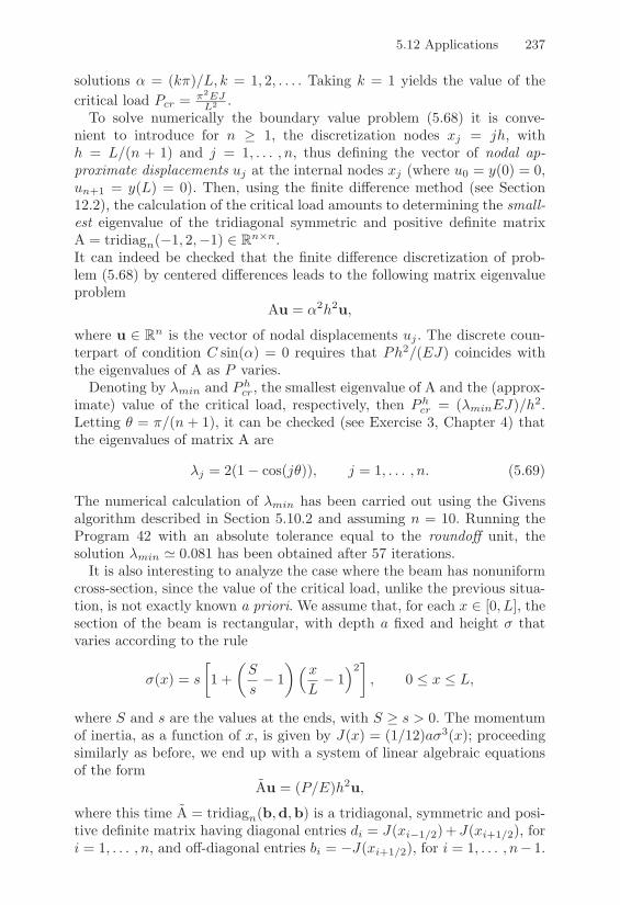
5.12 Applications 237
solutions " = (k&)/L, k = 1, 2, . . . . Taking k = 1 yields the value of thecritical load Pcr = "2EJ
L2 .To solve numerically the boundary value problem (5.68) it is conve-
nient to introduce for n ) 1, the discretization nodes xj = jh, withh = L/(n + 1) and j = 1, . . . , n, thus defining the vector of nodal ap-proximate displacements uj at the internal nodes xj (where u0 = y(0) = 0,un+1 = y(L) = 0). Then, using the finite di!erence method (see Section12.2), the calculation of the critical load amounts to determining the small-est eigenvalue of the tridiagonal symmetric and positive definite matrixA = tridiagn("1, 2,"1) ! Rn!n.It can indeed be checked that the finite di!erence discretization of prob-lem (5.68) by centered di!erences leads to the following matrix eigenvalueproblem
Au = "2h2u,
where u ! Rn is the vector of nodal displacements uj . The discrete coun-terpart of condition C sin(") = 0 requires that Ph2/(EJ) coincides withthe eigenvalues of A as P varies.
Denoting by $min and Phcr, the smallest eigenvalue of A and the (approx-
imate) value of the critical load, respectively, then Phcr = ($minEJ)/h2.
Letting ! = &/(n + 1), it can be checked (see Exercise 3, Chapter 4) thatthe eigenvalues of matrix A are
$j = 2(1" cos(j!)), j = 1, . . . , n. (5.69)
The numerical calculation of $min has been carried out using the Givensalgorithm described in Section 5.10.2 and assuming n = 10. Running theProgram 42 with an absolute tolerance equal to the roundo! unit, thesolution $min 1 0.081 has been obtained after 57 iterations.
It is also interesting to analyze the case where the beam has nonuniformcross-section, since the value of the critical load, unlike the previous situa-tion, is not exactly known a priori. We assume that, for each x ! [0, L], thesection of the beam is rectangular, with depth a fixed and height ( thatvaries according to the rule
((x) = s
-1 +
4S
s" 1
5K x
L" 1
L2., 0 & x & L,
where S and s are the values at the ends, with S ) s > 0. The momentumof inertia, as a function of x, is given by J(x) = (1/12)a(3(x); proceedingsimilarly as before, we end up with a system of linear algebraic equationsof the form
Au = (P/E)h2u,
where this time A = tridiagn(b,d,b) is a tridiagonal, symmetric and posi-tive definite matrix having diagonal entries di = J(xi"1/2)+J(xi+1/2), fori = 1, . . . , n, and o!-diagonal entries bi = "J(xi+1/2), for i = 1, . . . , n" 1.

238 5. Approximation of Eigenvalues and Eigenvectors
Assume the following values of the parameters: a = 0.4 [m], s = a, S =0.5 [m] and L = 10 [m]. To ensure a correct dimensional comparison, wehave multiplied by J = a4/12 the smallest eigenvalue of the matrix A in theuniform case (corresponding to S = s = a), obtaining $min = 1.7283 ·10"4.Running Program 42, with n = 10, yields in the nonuniform case the value$min = 2.243 · 10"4. This result confirms that the critical load increasesfor a beam having a wider section at x = 0, that is, the structure entersthe instability regime for higher values of the load than in the uniformcross-section case.
5.12.2 Free Dynamic Vibration of a BridgeWe are concerned with the analysis of the free response of a bridge whoseschematic structure is shown in Figure 5.5. The number of the nodes ofthe structure is equal to 2n while the number of the beams is 5n. Eachhorizontal and vertical beam has a mass equal to m while the diagonalbeams have mass equal to m
/2. The sti!ness of each beam is represented
by the spring constant 2. The nodes labeled by “0” and “2n + 1” areconstrained to ground.
2n + 1
n + 2 2n" 2 2n" 1n + 3n + 1 2n
0
1 2 3 n" 2 n" 1 n
FIGURE 5.5. Schematic structure of a bridge
Denoting by x and y the vectors of the 2n nodal horizontal and verticaldisplacements the free response of the bridge can be studied by solving thegeneralized eigenvalue problems
Mx = $Kx, My = $Ky, (5.70)
where M = mdiag2n(",b,", ',b, '), where " = 3 +/
2, b = (#, . . . ,#)T !Rn"2 with # = 3/2 +
/2 and ' = 1 +
/2,
K = 2
4K11 K12K12 K11
5
for a positive constant 2 and where K12 = tridiagn("1,"1,"1), K11 =tridiagn("1,d,"1) with d = (4, 5, . . . , 5, 4)T ! Rn. The diagonal matrixM is the mass matrix while the symmetric and positive definite matrix Kis the sti!ness matrix.

5.12 Applications 239
0 10 20 30 40 50 60 70 80 90 1000
10
20
30
40
50
60
70
80
90
100
FIGURE 5.6. Iterations number of the Lanczos method and of the inverse powermethod versus the size 2n of matrix C. The solid and the dash-dotted curvesrefer to the inverse power method (for #2n and #2n%1 respectively), while thedashed and the dotted curves refer to the Lanczos method (still for #2n and#2n%1, respectively)
For k = 1, . . . , 2n we denote by ($k, zk) any eigenvalue/eigenvector pairof (5.70) and call 0k =
/$k the natural frequencies and zk the modes of
vibration of the bridge. The study of the free vibrations is of primary im-portance in the design of a structure like a bridge or a multi-story building.Indeed, if the excitation frequency of an external force (vehicles, wind or,even worse, an earthquake) coincides with one of the natural frequencies ofthe structure then a condition of resonance occurs and, as a result, largeoscillations may dangerously arise.
Let us now deal with the numerical solution of the matrix eigenvalueproblem (5.70). For this purpose we introduce the change of variable z =M1/2x (or z = M1/2y) so that each generalized eigenvalue problem in (5.70)can be conveniently reformulated as
Cz = $z
where $ = 1/$ and the matrix C = M"1/2KM"1/2 is symmetric positivedefinite. This property allows us to use the Lanczos method described inSection 5.11 and also ensures quadratic convergence of the power iterations(see Section 5.11).
We approximate the first two subdominant eigenvalues $2n and $2n"1of the matrix C (i.e., its smallest and second smallest eigenvalues) in thecase m = 2 = 1 using the deflation procedure considered in Remark 5.3.The inverse power iteration and the Lanczos method are compared in thecomputation of $2n and $2n"1 in Figure 5.6.
The results show the superiority of the Lanczos method over the inverseiterations only when the matrix C is of small size. This is to be ascribedto the fact that, as n grows, the progressive influence of the rounding er-
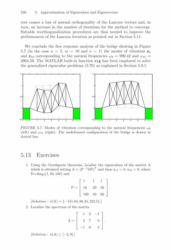
240 5. Approximation of Eigenvalues and Eigenvectors
rors causes a loss of mutual orthogonality of the Lanczos vectors and, inturn, an increase in the number of iterations for the method to converge.Suitable reorthogonalization procedures are thus needed to improve theperformances of the Lanczos iteration as pointed out in Section 5.11.
We conclude the free response analysis of the bridge showing in Figure5.7 (in the case n = 5, m = 10 and 2 = 1) the modes of vibration z8and z10 corresponding to the natural frequencies 08 = 990.42 and 010 =2904.59. The MATLAB built-in function eig has been employed to solvethe generalized eigenvalue problems (5.70) as explained in Section 5.9.1.
!1 0 1 2 3 4 5 6 7!0.5
0
0.5
1
1.5
!1 0 1 2 3 4 5 6 7!0.5
0
0.5
1
1.5
FIGURE 5.7. Modes of vibration corresponding to the natural frequencies -8
(left) and -10 (right). The undeformed configuration of the bridge is drawn indotted line
5.13 Exercises1. Using the Gershgorin theorems, localize the eigenvalues of the matrix A
which is obtained setting A = (P%1DP)T and then a13 = 0, a23 = 0, whereD=diag3(1, 50, 100) and
P =
"
##$
1 1 1
10 20 30
100 50 60
%
&&' .
[Solution : '(A) = {%151.84, 80.34, 222.5}.]2. Localize the spectrum of the matrix
A =
"
##$
1 2 %1
2 7 0
%1 0 5
%
&&' .
[Solution : '(A) 5 [%2, 9].]
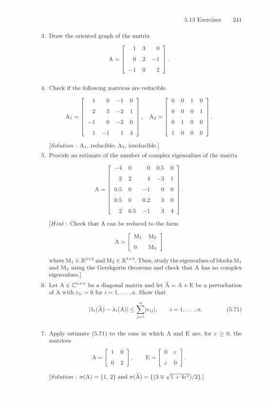
5.13 Exercises 241
3. Draw the oriented graph of the matrix
A =
"
##$
1 3 0
0 2 %1
%1 0 2
%
&&' .
4. Check if the following matrices are reducible.
A1 =
"
#####$
1 0 %1 0
2 3 %2 1
%1 0 %2 0
1 %1 1 4
%
&&&&&', A2 =
"
#####$
0 0 1 0
0 0 0 1
0 1 0 0
1 0 0 0
%
&&&&&'.
[Solution : A1, reducible; A2, irreducible.]
5. Provide an estimate of the number of complex eigenvalues of the matrix
A =
"
########$
%4 0 0 0.5 0
2 2 4 %3 1
0.5 0 %1 0 0
0.5 0 0.2 3 0
2 0.5 %1 3 4
%
&&&&&&&&'
.
[Hint : Check that A can be reduced to the form
A =
NM1 M2
0 M3
O
where M1 / R2&2 and M2 / R3&3. Then, study the eigenvalues of blocks M1
and M2 using the Gershgorin theorems and check that A has no complexeigenvalues.]
6. Let A / Cn&n be a diagonal matrix and let DA = A + E be a perturbationof A with eii = 0 for i = 1, . . . , n. Show that
|#i(DA)% #i(A)| "n(
j=1
|eij |, i = 1, . . . , n. (5.71)
7. Apply estimate (5.71) to the case in which A and E are, for & ! 0, thematrices
A =
N1 0
0 2
O
, E =
N0 &
& 0
O
.
[Solution : '(A) = {1, 2} and '(DA) = {(36'
1 + 4&2)/2}.]

242 5. Approximation of Eigenvalues and Eigenvectors
8. Check that finding the zeros of a polynomial of degree " n with real coef-ficients
pn(x) =n(
k=0
akxk = a0 + a1x + ... + anx
n, an $= 0, ak / R, k = 0, . . . n
is equivalent to determining the spectrum of the Frobenius matrix C /Rn&n associated with pn (known as the companion matrix)
C =
"
#####$
%(an%1/an) %(an%2/an) . . . %(a1/an) %(a0/an)1 0 . . . 0 00 1 . . . 0 0...
.... . .
......
0 0 . . . 1 0
%
&&&&&'.(5.72)
An important consequence of the result above is that, due to Abel’s theo-rem, there exist in general no direct methods for computing the eigenvaluesof a given matrix, for n ! 5.
9. Show that if matrix A / Cn&n admits eigenvalue/eigenvector pairs (#,x),then the matrix UHAU, with U unitary, admits eigenvalue/eigenvectorpairs
8#,UHx
9. (Similarity transformation using an orthogonal matrix).
10. Suppose that all the assumptions needed to apply the power method aresatisfied except for the requirement $1 $= 0 (see Section 5.3.1). Show thatin such a case the sequence (5.17) converges to the eigenvalue/eigenvectorpair (#2,x2). Then, study experimentally the behaviour of the method,computing the pair (#1,x1) for the matrix
A =
"
##$
1 %1 2
%2 0 5
6 %3 6
%
&&' .
For this, use Program 26, taking q(0) = 1T /'
3 and q(0) = w(0)/&w(0)&2,respectively, where w(0) = (1/3)x2 % (2/3)x3.[Solution : #1 = 5, #2 = 3, #3 = %1 and x1 = [5, 16, 18]T , x2 = [1, 6, 4]T ,x3 = [5, 16, 18]T .]
11. Show that the companion matrix associated with the polynomial pn(x) =xn + anx
n%1 + . . . + a1, can be written in the alternative form (5.72)
A =
"
######$
0 a1 0%1 0 a2
. . .. . .
. . .%1 0 an%1
0 %1 an
%
&&&&&&'.
12. (From [FF63]) Suppose that a real matrix A / Rn&n has two maximummodule complex eigenvalues given by #1 = %ei# and #2 = %e%i#, with

5.13 Exercises 243
. $= 0. Assume, moreover, that the remaining eigenvalues have modulesless than %. The power method can then be modified as follows:let q(0) be a real vector and q(k) be the vector provided by the powermethod without normalization. Then, set xk = q(k)
n0 for some n0, with1 " n0 " n. Prove that
%2 =xkxk+2 % x2
k+1
xk%1xk+1 % x2k
+ O4
%&k
5,
cos(.) =%xk%1 + r%1xk+1
2xk+ O
4
%&k
5.
[Hint : first, show that
xk = C(%k cos(k. + $)) + O4
%&k
5,
where $ depends on the components of the initial vector along the direc-tions of the eigenvectors associated with #1 and #2.]
13. Apply the modified power method of Exercise 12 to the matrix
A =
"
$1 % 1
414
1 0 00 1 0
%
' ,
and compare the obtained results with those yielded by the standard powermethod.
14. (Taken from [Dem97]). Apply the QR iteration with double shift to com-pute the eigenvalues of the matrix
A =
"
$0 0 11 0 00 1 0
%
' .
Run Program 37 setting toll=eps, itmax=100 and comment about theform of the obtained matrix T(iter) after iter iterations of the algorithm.[Solution : the eigenvalues of A are the solution of #3 % 1 = 0, i.e.,'(A) =
/1,%1/2 ±
'3/2i
0. After iter=100 iterations, Program 37 yields
the matrix
T(100) =
"
$0 0 %11 0 00 %1 0
%
' ,
which means that the QR iteration leaves A unchanged (except for signchanges that are non relevant for eigenvalues computation). This is a simplebut glaring example of matrix for which the QR method with double shiftfails to converge.]

6Rootfinding for Nonlinear Equations
This chapter deals with the numerical approximation of the zeros of a real-valued function of one variable, that is
given f : I = (a, b) 7 R ( R, find " ! C such that f(") = 0. (6.1)
The analysis of problem (6.1) in the case of systems of nonlinear equationswill be addressed in Chapter 7.
Methods for the numerical approximation of a zero of f are usually iter-ative. The aim is to generate a sequence of values x(k) such that
limk&$
x(k) = ".
The convergence of the iteration is characterized by the following definition.
Definition 6.1 A sequence/x(k)0 generated by a numerical method is
said to converge to " with order p ) 1 if
-C > 0 :|x(k+1) " "||x(k) " "|p
& C, #k ) k0, (6.2)
where k0 ) 0 is a suitable integer. In such a case, the method is said to beof order p. Notice that if p is equal to 1, in order for x(k) to converge to" it is necessary that C < 1 in (6.2). In such an event, the constant C iscalled the convergence factor of the method. !
Unlike the case of linear systems, convergence of iterative methods forrootfinding of nonlinear equations depends in general on the choice of the

246 6. Rootfinding for Nonlinear Equations
initial datum x(0). This allows for establishing only local convergence re-sults, that is, holding for any x(0) which belongs to a suitable neighborhoodof the root ". Methods for which convergence to " holds for any choice ofx(0) in the interval I, are said to be globally convergent to ".
6.1 Conditioning of a Nonlinear Equation
Consider the nonlinear equation f(x) = 1(x) " d = 0 and assume that fis a continuously di!erentiable function. Let us analyze the sensitivity offinding the roots of f with respect to changes in the datum d.
The problem is well posed only if the function 1 is invertible. In such acase, indeed, one gets " = 1"1(d) from which, using the notation of Chapter2, the resolvent G is 1"1. On the other hand, (1"1)*(d) = 1/1*("), so thatformula (2.7) for the approximate condition number (relative and absolute)yields
K(d) 1 |d||"||f *(")| , Kabs(d) 1
1|f *(")| . (6.3)
The problem is thus ill-conditioned when f *(") is “small” and well-condi-tioned if f *(") is “large”.
The analysis which leads to (6.3) can be generalized to the case in which" is a root of f with multiplicity m > 1 as follows. Expanding 1 in a Taylorseries around " up to the m-th order term, we get
d + %d = 1("+ %") = 1(") +m(
k=1
1(k)(")k!
(%")k + o((%")m).
Since 1(k)(") = 0 for k = 1, . . . ,m" 1, we obtain
%d = f (m)(")(%")m/m!
so that an approximation to the absolute condition number is
Kabs(d) 1>>>>
m!%df (m)(")
>>>>1/m 1
|%d| . (6.4)
Notice that (6.3) is the special case of (6.4) where m = 1. From this it alsofollows that, even if %d is su"ciently small to make |m!%d/f (m)(")| < 1,Kabs(d) could nevertheless be a large number. We therefore conclude thatthe problem of rootfinding of a nonlinear equation is well-conditioned if "is a simple root and |f *(")| is definitely di!erent from zero, ill-conditionedotherwise.
Let us now consider the following problem, which is closely connectedwith the previous analysis. Assume d = 0 and let " be a simple root of f ;
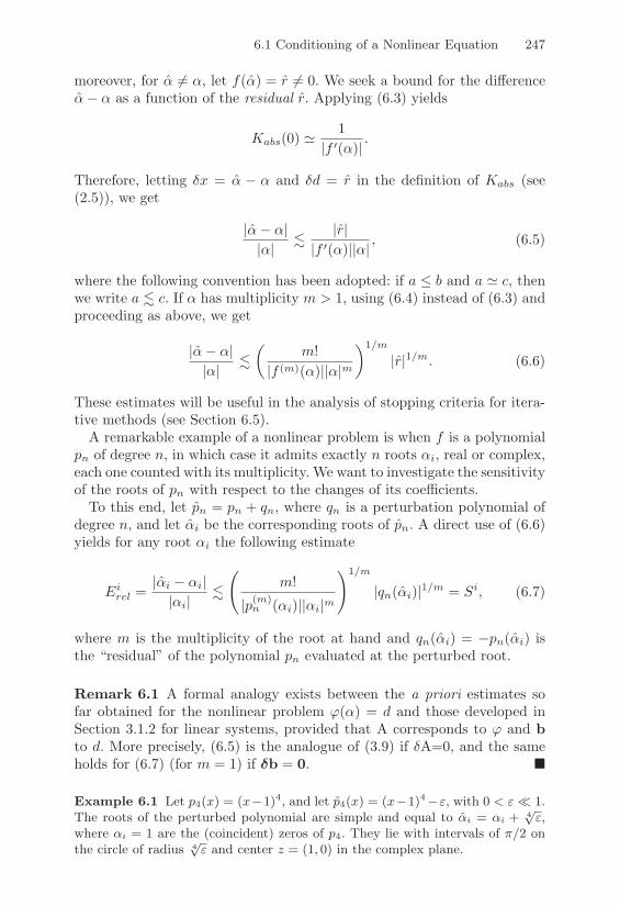
6.1 Conditioning of a Nonlinear Equation 247
moreover, for " '= ", let f(") = r '= 0. We seek a bound for the di!erence"" " as a function of the residual r. Applying (6.3) yields
Kabs(0) 1 1|f *(")| .
Therefore, letting %x = " " " and %d = r in the definition of Kabs (see(2.5)), we get
|"" "||"| " |r|
|f *(")||"| , (6.5)
where the following convention has been adopted: if a & b and a 1 c, thenwe write a " c. If " has multiplicity m > 1, using (6.4) instead of (6.3) andproceeding as above, we get
|"" "||"| "
4m!
|f (m)(")||"|m
51/m
|r|1/m. (6.6)
These estimates will be useful in the analysis of stopping criteria for itera-tive methods (see Section 6.5).
A remarkable example of a nonlinear problem is when f is a polynomialpn of degree n, in which case it admits exactly n roots "i, real or complex,each one counted with its multiplicity. We want to investigate the sensitivityof the roots of pn with respect to the changes of its coe"cients.
To this end, let pn = pn + qn, where qn is a perturbation polynomial ofdegree n, and let "i be the corresponding roots of pn. A direct use of (6.6)yields for any root "i the following estimate
Eirel =
|"i " "i||"i|
"6
m!
|p(m)n ("i)||"i|m
71/m
|qn("i)|1/m = Si, (6.7)
where m is the multiplicity of the root at hand and qn("i) = "pn("i) isthe “residual” of the polynomial pn evaluated at the perturbed root.
Remark 6.1 A formal analogy exists between the a priori estimates sofar obtained for the nonlinear problem 1(") = d and those developed inSection 3.1.2 for linear systems, provided that A corresponds to 1 and bto d. More precisely, (6.5) is the analogue of (3.9) if %A=0, and the sameholds for (6.7) (for m = 1) if "b = 0. !
Example 6.1 Let p4(x) = (x%1)4, and let p4(x) = (x%1)4%&, with 0 < &2 1.The roots of the perturbed polynomial are simple and equal to $i = $i + 4
'&,
where $i = 1 are the (coincident) zeros of p4. They lie with intervals of +/2 onthe circle of radius 4
'& and center z = (1, 0) in the complex plane.

248 6. Rootfinding for Nonlinear Equations
The problem is stable (that is lim'$0 $i = 1), but is ill-conditioned since
|$i % $i||$i|
= 4'&, i = 1, . . . 4,
For example, if & = 10%4 the relative change is 10%1. Notice that the right-sideof (6.7) is just 4
'&, so that, in this case, (6.7) becomes an equality. •
Example 6.2 (Wilkinson). Consider the following polynomial
p10(x) = (10k=1(x + k) = x10 + 55x9 + . . . + 10!.
Let p10 = p10 + &x9, with & = 2%23 0 1.2 · 10%7. Let us study the conditioning offinding the roots of p10. Using (6.7) with m = 1, we report for i = 1, . . . , 10 inTable 6.1 the relative errors Ei
rel and the corresponding estimates Si.These results show that the problem is ill-conditioned, since the maximum
relative error for the root $8 = %8 is three orders of magnitude larger thanthe corresponding absolute perturbation. Moreover, excellent agreement can beobserved between the a priori estimate and the actual relative error. •
i Eirel Si i Ei
rel Si
1 3.039 · 10"13 3.285 · 10"13 6 6.956 · 10"5 6.956 · 10"5
2 7.562 · 10"10 7.568 · 10"10 7 1.589 · 10"4 1.588 · 10"4
3 7.758 · 10"8 7.759 · 10"8 8 1.984 · 10"4 1.987 · 10"4
4 1.808 · 10"6 1.808 · 10"6 9 1.273 · 10"4 1.271 · 10"4
5 1.616 · 10"5 1.616 · 10"5 10 3.283 · 10"5 3.286 · 10"5
TABLE 6.1. Relative error and estimated error using (6.7) for the Wilkinsonpolynomial of degree 10
6.2 A Geometric Approach to Rootfinding
In this section we introduce the following methods for finding roots: thebisection method, the chord method, the secant method, the false position(or Regula Falsi) method and Newton’s method. The order of the presen-tation reflects the growing complexity of the algorithms. In the case of thebisection method, indeed, the only information that is being used is the signof the function f at the end points of any bisection (sub)interval, whilstthe remaining algorithms also take into account the values of the functionand/or its derivative.
6.2.1 The Bisection MethodThe bisection method is based on the following property.

6.2 A Geometric Approach to Rootfinding 249
Property 6.1 (theorem of zeros for continuous functions) Given acontinuous function f : [a, b] ( R, such that f(a)f(b) < 0, then - " ! (a, b)such that f(") = 0.
Starting from I0 = [a, b], the bisection method generates a sequence ofsubintervals Ik = [a(k), b(k)], k ) 0, with Ik * Ik"1, k ) 1, and enjoys theproperty that f(a(k))f(b(k)) < 0. Precisely, we set a(0) = a, b(0) = b andx(0) = (a(0) + b(0))/2; then, for k ) 0:
set a(k+1) = a(k), b(k+1) = x(k) if f(x(k))f(a(k)) < 0;
set a(k+1) = x(k), b(k+1) = b(k) if f(x(k))f(b(k)) < 0;
finally, set x(k+1) = (a(k+1) + b(k+1))/2.
x(1)x
y
f(x)
a b
!
I1
I0
x(0)
0 5 10 15 20 25 3010
!12
10!10
10!8
10!6
10!4
10!2
100
FIGURE 6.1. The bisection method. The first two steps (left); convergence historyfor the Example 6.3 (right). The number of iterations and the absolute error asa function of k are reported on the x- and y-axis, respectively
The bisection iteration terminates at the m-th step for which |x(m)""| &|Im| & +, where + is a fixed tolerance and |Im| is the length of Im. As forthe speed of convergence of the bisection method, notice that |I0| = b" a,while
|Ik| = |I0|/2k = (b" a)/2k, k ) 0. (6.8)
Denoting by e(k) = x(k) " " the absolute error at step k, from (6.8) itfollows that |e(k)| & (b" a)/2k, k ) 0, which implies limk&$ |e(k)| = 0.
The bisection method is therefore globally convergent. Moreover, to get|x(m) " "| & + we must take
m ) log2(b" a)" log2(+) =log((b" a)/+)
log(2)1 log((b" a)/+)
0.6931. (6.9)
In particular, to gain a significant figure in the accuracy of the approxi-mation of the root (that is, to have |x(k) " "| = |x(j) " "|/10), one needs

250 6. Rootfinding for Nonlinear Equations
k"j = log2(10) 1 3.32 bisections. This singles out the bisection method asan algorithm of certain, but slow, convergence. We must also point out thatthe bisection method does not generally guarantee a monotone reductionof the absolute error between two successive iterations, that is, we cannotensure a priori that
|e(k+1)| &Mk|e(k)|, for any k ) 0, (6.10)
with Mk < 1. For this purpose, consider the situation depicted in Figure6.1 (left), where clearly |e(1)| > |e(0)|. Failure to satisfy (6.10) does notallow for qualifying the bisection method as a method of order 1, in thesense of Definition 6.1.
Example 6.3 Let us check the convergence properties of the bisection methodin the approximation of the root $ 0 0.9062 of the Legendre polynomial of degree5
L5(x) =x8(63x4 % 70x2 + 15),
whose roots lie within the interval (%1, 1) (see Section 10.1.2). Program 46 hasbeen run taking a = 0.6, b = 1 (whence, L5(a) · L5(b) < 0), nmax = 100,toll = 10%10 and has reached convergence in 32 iterations, this agrees withthe theoretical estimate (6.9) (indeed, m ! 31.8974). The convergence history isreported in Figure 6.1 (right) and shows an (average) reduction of the error by afactor of two, with an oscillating behavior of the sequence {x(k)}. •
The slow reduction of the error suggests employing the bisection methodas an “approaching” technique to the root. Indeed, taking few bisectionsteps, a reasonable approximation to " is obtained, starting from which ahigher order method can be successfully used for a rapid convergence tothe solution within the fixed tolerance. An example of such a procedurewill be addressed in Section 6.7.1.
The bisection algorithm is implemented in Program 46. The input pa-rameters, here and in the remainder of this chapter, have the followingmeaning: a and b denote the end points of the search interval, fun is thevariable containing the expression of the function f , toll is a fixed toler-ance and nmax is the maximum admissible number of steps for the iterativeprocess.
In the output vectors xvect, xdif and fx the sequences {x(k)}, {|x(k+1)"x(k)|} and {f(x(k))}, for k ) 0, are respectively stored, while nit denotesthe number of iterations needed to satisfy the stopping criteria. In the caseof the bisection method, the code returns as soon as the half-length of thesearch interval is less than toll.
Program 46 - bisect : Bisection method
function [xvect,xdif,fx,nit]=bisect(a,b,toll,nmax,fun)err=toll+1; nit=0; xvect=[]; fx=[]; xdif=[];while (nit < nmax & err > toll)
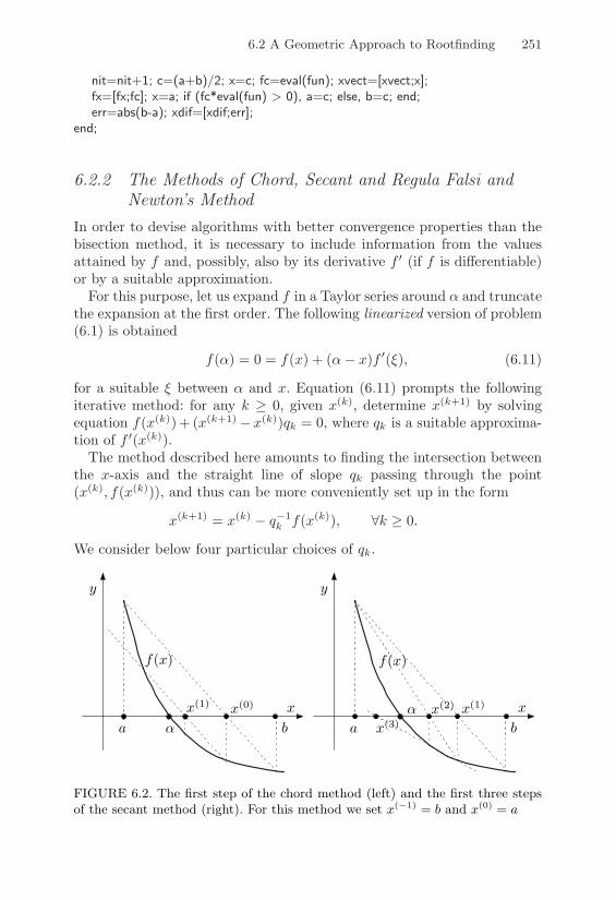
6.2 A Geometric Approach to Rootfinding 251
nit=nit+1; c=(a+b)/2; x=c; fc=eval(fun); xvect=[xvect;x];fx=[fx;fc]; x=a; if (fc*eval(fun) > 0), a=c; else, b=c; end;err=abs(b-a); xdif=[xdif;err];
end;
6.2.2 The Methods of Chord, Secant and Regula Falsi andNewton’s Method
In order to devise algorithms with better convergence properties than thebisection method, it is necessary to include information from the valuesattained by f and, possibly, also by its derivative f * (if f is di!erentiable)or by a suitable approximation.
For this purpose, let us expand f in a Taylor series around " and truncatethe expansion at the first order. The following linearized version of problem(6.1) is obtained
f(") = 0 = f(x) + ("" x)f *(*), (6.11)
for a suitable * between " and x. Equation (6.11) prompts the followingiterative method: for any k ) 0, given x(k), determine x(k+1) by solvingequation f(x(k))+ (x(k+1)"x(k))qk = 0, where qk is a suitable approxima-tion of f *(x(k)).
The method described here amounts to finding the intersection betweenthe x-axis and the straight line of slope qk passing through the point(x(k), f(x(k))), and thus can be more conveniently set up in the form
x(k+1) = x(k) " q"1k f(x(k)), #k ) 0.
We consider below four particular choices of qk.
f(x)
x(1)
y
ba
f(x)
x(0) x
y
ba
x(1) xx(2)"" x(3)
FIGURE 6.2. The first step of the chord method (left) and the first three stepsof the secant method (right). For this method we set x(%1) = b and x(0) = a
252 6. Rootfinding for Nonlinear Equations
The chord method. We let
qk = q =f(b)" f(a)
b" a, #k ) 0
from which, given an initial value x(0), the following recursive relation isobtained
x(k+1) = x(k) " b" a
f(b)" f(a)f(x(k)), k ) 0. (6.12)
In Section 6.3.1, we shall see that the sequence {x(k)} generated by (6.12)converges to the root " with order of convergence p = 1.
The secant method. We let
qk =f(x(k))" f(x(k"1))
x(k) " x(k"1) , #k ) 0 (6.13)
from which, giving two initial values x("1) and x(0), we obtain the followingrelation
x(k+1) = x(k) " x(k) " x(k"1)
f(x(k))" f(x(k"1))f(x(k)), k ) 0. (6.14)
If compared with the chord method, the iterative process (6.14) requiresan extra initial point x("1) and the corresponding function value f(x("1)),as well as, for any k, computing the incremental ratio (6.13). The benefitdue to the increase in the computational cost is the higher speed of con-vergence of the secant method, as stated in the following property whichcan be regarded as a first example of the local convergence theorem (for theproof see [IK66], pp. 99-101).
Property 6.2 Let f ! C2(J ), J being a suitable neighborhood of the root" and assume that f **(") '= 0. Then, if the initial data x("1) and x(0) arechosen in J su"ciently close to ", the sequence (6.14) converges to " withorder p = (1 +
/5)/2 1 1.63.
The Regula Falsi (or false position) method. This is a variant ofthe secant method in which, instead of selecting the secant line throughthe values (x(k), f(x(k)) and (x(k"1), f(x(k"1)), we take the one through(x(k), f(x(k)) and (x(k%), f(x(k%)), k* being the maximum index less than ksuch that f(x(k%)) · f(x(k)) < 0. Precisely, once two values x("1) and x(0)
have been found such that f(x("1)) · f(x(0)) < 0, we let
x(k+1) = x(k) " x(k) " x(k%)
f(x(k))" f(x(k%))f(x(k)), k ) 0. (6.15)

6.2 A Geometric Approach to Rootfinding 253
Having fixed an absolute tolerance +, the iteration (6.15) terminates at them-th step such that |f(x(m))| < +. Notice that the sequence of indices k*
is nondecreasing; therefore, in order to find at step k the new value of k*,it is not necessary to sweep all the sequence back, but it su"ces to stop atthe value of k* that has been determined at the previous step. We show inFigure 6.3 (left) the first two steps of (6.15) in the special case in whichx(k%) coincides with x("1) for any k ) 0.
The Regula Falsi method, though of the same complexity as the secantmethod, has linear convergence order (see, for example, [RR78], pp. 339-340). However, unlike the secant method, the iterates generated by (6.15)are all contained within the starting interval [x("1), x(0)].
In Figure 6.3 (right), the first two iterations of both the secant and RegulaFalsi methods are shown, starting from the same initial data x("1) and x(0).Notice that the iterate x(1) computed by the secant method coincides withthat computed by the Regula Falsi method, while the value x(2) computedby the former method (and denoted in the figure by x(2)
Sec) falls outside thesearching interval [x("1), x(0)].
In this respect, the Regula Falsi method, as well as the bisection method,can be regarded as a globally convergent method.
f(x)y
f(x)
x("1) x(0)
x
x(1)x(2)
y
x(0)
x
x("1) x(1)
x(2)
x(2)Sec
FIGURE 6.3. The first two steps of the Regula Falsi method for two di"erentfunctions
Newton’s method.Assuming that f ! C1(I) and that f *(") '= 0 (i.e., " is a simple root of f),if we let
qk = f *(x(k)), #k ) 0
and assign the initial value x(0), we obtain the so called Newton’s method
x(k+1) = x(k) " f(x(k))f *(x(k))
, k ) 0. (6.16)

254 6. Rootfinding for Nonlinear Equations
x(2)
a b
x
f(x)
y
x(1)
x(0)
0 5 10 15 20 25 30 35
10!15
10!10
10!5
100
(1)
(2)
(3)
(4)
FIGURE 6.4. The first two steps of Newton’s method (left); convergence historiesin Example 6.4 for the chord method (1), bisection method (2), secant method(3) and Newton’s method (4) (right). The number of iterations and the absoluteerror as a function of k are shown on the x-axis and y-axis, respectively
At the k-th iteration, Newton’s method requires the two functional evalu-ations f(x(k)) and f *(x(k)). The increasing computational cost with respectto the methods previously considered is more than compensated for by ahigher order of convergence, Newton’s method being of order 2 (see Section6.3.1).
Example 6.4 Let us compare the methods introduced so far for the approxima-tion of the root $ 0 0.5149 of the function f(x) = cos2(2x) % x2 in the interval(0, 1.5). The tolerance & on the absolute error has been taken equal to 10%10 andthe convergence histories are drawn in Figure 6.4 (right). For all methods, theinitial guess x(0) has been set equal to 0.75. For the secant method we chosex(%1) = 0.
The analysis of the results singles out the slow convergence of the chordmethod. The error curve for the Regula Falsi method is similar to that of se-cant method, thus it was not reported in Figure 6.4.
It is interesting to compare the performances of Newton’s and secant methods(both having order p > 1), in terms of their computational e"ort. It can indeedbe proven that it is more convenient to employ the secant method whenever thenumber of floating point operations to evaluate f ( are about twice those neededfor evaluating f (see [Atk89], pp. 71-73). In the example at hand, Newton’smethod converges to $ in 6 iterations, instead of 7, but the secant method takes94 flops instead of 177 flops required by Newton’s method. •
The chord, secant, Regula Falsi and Newton’s methods are implementedin Programs 47, 48, 49 and 50, respectively. Here and in the rest of thechapter, x0 and xm1 denote the initial data x(0) and x("1). In the case ofthe Regula Falsi method the stopping test checks is |f(x(k))| < toll, whilefor the other methods the test is |x(k+1) " x(k)| < toll. The string dfuncontains the expression of f * to be used in the Newton method.

6.2 A Geometric Approach to Rootfinding 255
Program 47 - chord : The chord method
function [xvect,xdif,fx,nit]=chord(a,b,x0,nmax,toll,fun)x=a; fa=eval(fun); x=b; fb=eval(fun); r=(fb-fa)/(b-a);err=toll+1; nit=0; xvect=x0; x=x0; fx=eval(fun); xdif=[];while (nit < nmax & err > toll),
nit=nit+1; x=xvect(nit); xn=x-fx(nit)/r; err=abs(xn-x);xdif=[xdif; err]; x=xn; xvect=[xvect;x]; fx=[fx;eval(fun)];
end;
Program 48 - secant : The secant method
function [xvect,xdif,fx,nit]=secant(xm1,x0,nmax,toll,fun)x=xm1; fxm1=eval(fun); xvect=[x]; fx=[fxm1]; x=x0; fx0=eval(fun);xvect=[xvect;x]; fx=[fx;fx0]; err=toll+1; nit=0; xdif=[];while (nit < nmax & err > toll),
nit=nit+1; x=x0-fx0*(x0-xm1)/(fx0-fxm1); xvect=[xvect;x];fnew=eval(fun); fx=[fx;fnew]; err=abs(x0-x); xdif=[xdif;err];xm1=x0; fxm1=fx0; x0=x; fx0=fnew;
end;
Program 49 - regfalsi : The Regula Falsi method
function [xvect,xdif,fx,nit]=regfalsi(xm1,x0,toll,nmax,fun)nit=0; x=xm1; f=eval(fun); fx=[f]; x=x0; f=eval(fun); fx=[fx, f];xvect=[xm1,x0]; xdif=[]; f=toll+1; kprime=1;while (nit < nmax & (abs(f) > toll),
nit=nit+1; dim=length(xvect);x=xvect(dim); fxk=eval(fun); xk=x; i=dim;while (i >= kprime), i=i-1; x=xvect(i); fxkpr=eval(fun);
if ((fxkpr*fxk) < 0), xkpr=x; kprime=i; break; end;end;x=xk-fxk*(xk-xkpr)/(fxk-fxkpr); xvect=[xvect, x]; f=eval(fun);fx=[fx, f]; err=abs(x-xkpr); xdif=[xdif, err];
end;
Program 50 - newton : Newton’s method
function [xvect,xdif,fx,nit]=newton(x0,nmax,toll,fun,dfun)err=toll+1; nit=0; xvect=x0; x=x0; fx=eval(fun); xdif=[];while (nit < nmax & err > toll),
nit=nit+1; x=xvect(nit); dfx=eval(dfun);if (dfx == 0), err=toll*1.e-10;
disp(’ Stop for vanishing dfun ’);else,
xn=x-fx(nit)/dfx; err=abs(xn-x); xdif=[xdif; err];x=xn; xvect=[xvect;x]; fx=[fx;eval(fun)];
256 6. Rootfinding for Nonlinear Equations
end;end;
6.2.3 The Dekker-Brent MethodThe Dekker-Brent method combines the bisection and secant methods, pro-viding a synthesis of the advantages of both. This algorithm carries out aniteration in which three abscissas a, b and c are present at each stage. Nor-mally, b is the latest iterate and closest approximation to the zero, a isthe previous iterate and c is the previous or an older iterate so that f(b)and f(c) have opposite signs. At all times b and c bracket the zero and|f(b)| & |f(c)|.
Once an interval [a, b] containing at least one root " of the functiony = f(x) is found with f(a)f(b) < 0, the algorithm generates a sequence ofvalues a, b and c such that " always lies between b and c and, at convergence,the half-length |c " b|/2 is less than a fixed tolerance. If the function f issu"ciently smooth around the desired root, then the order of convergenceof the algorithm is more than linear (see [Dek69], [Bre73] Chapter 4 and[Atk89], pp. 91-93).
In the following we describe the main lines of the algorithm as imple-mented in the MATLAB function fzero. Throughout the parameter d willbe a correction to the point b since it is best to arrange formulae so thatthey express the desired quantity as a small correction to a good approx-imation. For example, if the new value of b were computed as (b + c)/2(bisection step) a numerical cancellation might occur, while computing bas b + (c" b)/2 gives a more stable formula.Denote by + a suitable tolerance (usually the machine precision) and letc = b; then, the Dekker-Brent method proceeds as follows:
First, check if f(b) = 0. Should this be the case, the algorithm terminatesand returns b as the approximate zero of f . Otherwise, the following stepsare executed:
1. if f(b)f(c) > 0, set c = a, d = b" a and e = d.
2. If |f(c)| < |f(b)|, perform the exchanges a = b, b = c and c = a.
3. Set % = 2+max {|b|, 1} and m = (c" b)/2. If |m| & % or f(b) = 0 thenthe algorithm terminates and returns b as the approximate zero of f .
4. Choose bisection or interpolation.
(a) If |e| < % or |f(a)| & |f(b)| then a bisection step is taken, i.e., setd = m and e = m; otherwise, the interpolation step is executed.
(b) if a = c execute linear interpolation, i.e., compute the zero of thestraight line passing through the points (b, f(b)) and (c, f(c)) as
6.3 Fixed-point Iterations for Nonlinear Equations 257
a correction %b to the point b. This amounts to taking a step ofthe secant method on the interval having b and c as end points.If a '= c execute inverse quadratic interpolation, i.e., constructthe second-degree polynomial with respect to y, that interpo-lates at the points (f(a), a), (f(b), b) and (f(c), c) and its valueat y = 0 is computed as a correction %b to the point b. Noticethat at this stage the values f(a), f(b) and f(c) are di!erent onefrom the others, being |f(a)| > |f(b)|, f(b)f(c) < 0 and a '= c.Then the algorithm checks whether the point b + %b can be ac-cepted. This is a rather technical issue but essentially it amountsto ascertaining if the point is inside the current interval and nottoo close to the end points. This guarantees that the length ofthe interval decreases by a large factor when the function is wellbehaved. If the point is accepted then e = d and d = %b, i.e.,the interpolation is actually carried out, else a bisection step isexecuted by setting d = m and e = m.
5. The algorithm now updates the current iterate. Set a = b and if|d| > % then b = b + d else b = b + %sign(m) and go back to step 1.
Example 6.5 Let us consider the finding of roots of the function f considered inExample 6.4, taking & equal to the roundo! unit. The MATLAB function fzerohas been employed. It automatically determines the values a and b, starting froma given initial guess / provided by the user. Starting from / = 1.5, the algorithmfinds the values a = 0.3 and b = 2.1; convergence is achieved in 5 iterations andthe sequences of the values a, b, c and f(b) are reported in Table 6.2.
Notice that the tabulated values refer to the state of the algorithm before step3., and thus, in particular, after possible exchanges between a and b. •
k a b c f(b)0 2.1 0.3 2.1 0.59121 0.3 0.5235 0.3 "2.39 · 10"2
2 0.5235 0.5148 0.5235 3.11 · 10"4
3 0.5148 0.5149 0.5148 "8.8 · 10"7
4 0.5149 0.5149 0.5148 "3.07 · 10"11
TABLE 6.2. Solution of the equation cos2(2x) % x2 = 0 using the Dekker-Brentalgorithm. The integer k denotes the current iteration
6.3 Fixed-point Iterations for Nonlinear Equations
In this section a completely general framework for finding the roots of anonlinear function is provided. The method is based on the fact that, for agiven f : [a, b] ( R, it is always possible to transform the problem f(x) = 0

258 6. Rootfinding for Nonlinear Equations
into an equivalent problem x " 4(x) = 0, where the auxiliary function4 : [a, b] ( R has to be chosen in such a way that 4(") = " wheneverf(") = 0. Approximating the zeros of a function has thus become theproblem of finding the fixed points of the mapping 4, which is done by thefollowing iterative algorithm:given x(0), let
x(k+1) = 4(x(k)), k ) 0. (6.17)
We say that (6.17) is a fixed-point iteration and 4 is its associated iterationfunction. Sometimes, (6.17) is also referred to as Picard iteration or func-tional iteration for the solution of f(x) = 0. Notice that by constructionthe methods of the form (6.17) are strongly consistent in the sense of thedefinition given in Section 2.2.
The choice of 4 is not unique. For instance, any function of the form4(x) = x+ F (f(x)), where F is a continuous function such that F (0) = 0,is an admissible iteration function.The next two results provide su"cient conditions in order for the fixed-point method (6.17) to converge to the root " of problem (6.1). Theseconditions are stated precisely in the following theorem.
Theorem 6.1 (convergence of fixed-point iterations) Consider the se-quence x(k+1) = 4(x(k)), for k ) 0, being x(0) given. Assume that:
1. 4 : [a, b]( [a, b];
2. 4 ! C1([a, b]);
3. -K < 1 : |4*(x)| & K #x ! [a, b].
Then, 4 has a unique fixed point " in [a, b] and the sequence {x(k)} con-verges to " for any choice of x(0) ! [a, b]. Moreover, we have
limk&$
x(k+1) " "x(k) " "
= 4*("). (6.18)
Proof. The assumption 1. and the continuity of 3 ensure that the iterationfunction 3 has at least one fixed point in [a, b]. Assumption 3. states that 3 isa contraction mapping and ensures the uniqueness of the fixed point. Indeed,suppose that there exist two distinct values $1, $2 / [a, b] such that 3($1) = $1
and 3($2) = $2. Expanding 3 in a Taylor series around $1 and truncating it atfirst order, it follows that
|$2 % $1| = |3($2)% 3($1)| = |3((0)($2 % $1)| " K|$2 % $1| < |$2 % $1|,
for 0 / ($1,$2), from which it must necessarily be that $2 = $1.The convergence analysis for the sequence {x(k)} is again based on a Taylor
series expansion. Indeed, for any k ! 0 there exists a value 0(k) between $ andx(k) such that
x(k+1) % $ = 3(x(k))% 3($) = 3((0(k))(x(k) % $) (6.19)
6.3 Fixed-point Iterations for Nonlinear Equations 259
from which |x(k+1) % $| " K|x(k) % $| " Kk+1|x(0) % $| , 0 for k , #. Thus,x(k) converges to $ and (6.19) implies that
limk$!
x(k+1) % $
x(k) % $= lim
k$!3((0(k)) = 3(($),
that is (6.18). !
The quantity |4*(")| is called the asymptotic convergence factor and, inanalogy with the case of iterative methods for linear systems, the asymp-totic convergence rate can be defined as
R = " log1
|4*(")| . (6.20)
Theorem 6.1 ensures convergence of the sequence {x(k)} to the root " forany choice of the initial value x(0) ! [a, b]. As such, it represents an exampleof a global convergence result.
In practice, however, it is often quite di"cult to determine a priori thewidth of the interval [a, b]; in such a case the following convergence resultcan be useful (see for the proof, [OR70]).
Property 6.3 (Ostrowski theorem) Let " be a fixed point of a func-tion 4, which is continuous and di!erentiable in a neighborhood J of ". If|4*(")| < 1 then there exists % > 0 such that the sequence {x(k)} convergesto ", for any x(0) such that |x(0) " "| < %.
Remark 6.2 If |4*(")| > 1 it follows from (6.19) that if x(n) is su"cientlyclose to ", so that |4*(x(n))| > 1, then |" " x(n+1)| > |" " x(n)|, thusno convergence is possible. In the case |4*(")| = 1 no general conclusioncan be stated since both convergence and nonconvergence may be possible,depending on the problem at hand. !
Example 6.6 Let 3(x) = x% x3, which admits $ = 0 as fixed point. Although3(($) = 1, if x(0) / [%1, 1] then x(k) / (%1, 1) for k ! 1 and it converges (veryslowly) to $ (if x(0) = ±1, we even have x(k) = $ for any k ! 1). Starting fromx(0) = 1/2 the absolute error after 2000 iterations is 0.0158. Let now 3(x) = x+x3
having also $ = 0 as fixed point. Again, 3(($) = 1 but in this case the sequencex(k) diverges for any choice x(0) $= 0. •
We say that a fixed-point method has order p (p non necessarily being aninteger) if the sequence that is generated by the method converges to thefixed point " with order p according to Definition 6.1.
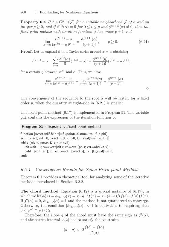
260 6. Rootfinding for Nonlinear Equations
Property 6.4 If 4 ! Cp+1(J ) for a suitable neighborhood J of " and aninteger p ) 0, and if 4(i)(") = 0 for 0 & i & p and 4(p+1)(") '= 0, then thefixed-point method with iteration function 4 has order p + 1 and
limk&$
x(k+1) " "(x(k) " ")p+1 =
4(p+1)(")(p + 1)!
, p ) 0. (6.21)
Proof. Let us expand 3 in a Taylor series around x = $ obtaining
x(k+1) % $ =p(
i=0
3(i)($)i!
(x(k) % $)i +3(p+1)(0)(p + 1)!
(x(k) % $)p+1,
for a certain 0 between x(k) and $. Thus, we have
limk$!
x(k+1) % $
(x(k) % $)p+1 = limk$!
3(p+1)(0)(p + 1)!
=3(p+1)($)(p + 1)!
.
!
The convergence of the sequence to the root " will be faster, for a fixedorder p, when the quantity at right-side in (6.21) is smaller.
The fixed-point method (6.17) is implemented in Program 51. The variablephi contains the expression of the iteration function 4.
Program 51 - fixpoint : Fixed-point method
function [xvect,xdif,fx,nit]=fixpoint(x0,nmax,toll,fun,phi)err=toll+1; nit=0; xvect=x0; x=x0; fx=eval(fun); xdif=[];while (nit < nmax & err > toll),
nit=nit+1; x=xvect(nit); xn=eval(phi); err=abs(xn-x);xdif=[xdif; err]; x=xn; xvect=[xvect;x]; fx=[fx;eval(fun)];
end;
6.3.1 Convergence Results for Some Fixed-point MethodsTheorem 6.1 provides a theoretical tool for analyzing some of the iterativemethods introduced in Section 6.2.2.
The chord method. Equation (6.12) is a special instance of (6.17), inwhich we let 4(x) = 4chord(x) = x"q"1f(x) = x"(b"a)/(f(b)"f(a))f(x).If f *(") = 0, 4*chord(") = 1 and the method is not guaranteed to converge.Otherwise, the condition |4*chord(")| < 1 is equivalent to requiring that0 < q"1f *(") < 2.
Therefore, the slope q of the chord must have the same sign as f *("),and the search interval [a, b] has to satisfy the constraint
(b" a) < 2f(b)" f(a)
f *(").

6.4 Zeros of Algebraic Equations 261
The chord method converges in one iteration if f is a straight line, otherwiseit converges linearly, apart the (lucky) case when f *(") = (f(b)"f(a))/(b"a), for which 4*chord(") = 0.
Newton’s method. Equation (6.16) can be cast in the general framework(6.17) letting
4Newt(x) = x" f(x)f *(x)
.
Assuming f *(") '= 0 (that is, " is a simple root)
4*Newt(") = 0, 4**Newt(") =f **(")f *(")
.
If the root " has multiplicity m > 1, then the method (6.16) is no longersecond-order convergent. Indeed we have (see Exercise 2)
4*Newt(") = 1" 1m. (6.22)
If the value of m is known a priori, then the quadratic convergence ofNewton’s method can be recovered by resorting to the so-called modifiedNewton’s method
x(k+1) = x(k) "mf(x(k))f *(x(k))
, k ) 0. (6.23)
To check the convergence order of the iteration (6.23), see Exercise 2.
6.4 Zeros of Algebraic Equations
In this section we address the special case in which f is a polynomial ofdegree n ) 0, i.e., a function of the form
pn(x) =n(
k=0
akxk, (6.24)
where ak ! R are given coe"cients.The above representation of pn is not the only one possible. Actually,
one can also write
pn(x) = an(x" "1)m1 ...(x" "k)mk ,k(
l=1
ml = n
where "i and mi denote the i-th root of pn and its multiplicity, respectively.Other representations are available as well, see Section 6.4.1.
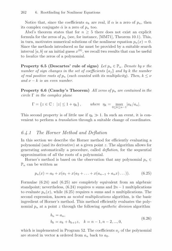
262 6. Rootfinding for Nonlinear Equations
Notice that, since the coe"cients ak are real, if " is a zero of pn, thenits complex conjugate " is a zero of pn too.
Abel’s theorem states that for n ) 5 there does not exist an explicitformula for the zeros of pn (see, for instance, [MM71], Theorem 10.1). This,in turn, motivates numerical solutions of the nonlinear equation pn(x) = 0.Since the methods introduced so far must be provided by a suitable searchinterval [a, b] or an initial guess x(0), we recall two results that can be usefulto localize the zeros of a polynomial.
Property 6.5 (Descartes’ rule of signs) Let pn ! Pn. Denote by 3 thenumber of sign changes in the set of coe"cients {aj} and by k the numberof real positive roots of pn (each counted with its multiplicity). Then, k & 3and 3 " k is an even number.
Property 6.6 (Cauchy’s Theorem) All zeros of pn are contained in thecircle * in the complex plane
* = {z ! C : |z| & 1 + -k} , where -k = max0%k%n"1
|ak/an|.
This second property is of little use if -k 4 1. In such an event, it is con-venient to perform a translation through a suitable change of coordinates.
6.4.1 The Horner Method and DeflationIn this section we describe the Horner method for e"ciently evaluating apolynomial (and its derivative) at a given point z. The algorithm allows forgenerating automatically a procedure, called deflation, for the sequentialapproximation of all the roots of a polynomial.
Horner’s method is based on the observation that any polynomial pn !Pn can be written as
pn(x) = a0 + x(a1 + x(a2 + . . . + x(an"1 + anx) . . . )). (6.25)
Formulae (6.24) and (6.25) are completely equivalent from an algebraicstandpoint; nevertheless, (6.24) requires n sums and 2n" 1 multiplicationsto evaluate pn(x), while (6.25) requires n sums and n multiplications. Thesecond expression, known as nested multiplications algorithm, is the basicingredient of Horner’s method. This method e"ciently evaluates the poly-nomial pn at a point z through the following synthetic division algorithm
bn = an,
bk = ak + bk+1z, k = n" 1, n" 2, ..., 0,(6.26)
which is implemented in Program 52. The coe"cients aj of the polynomialare stored in vector a ordered from an back to a0.
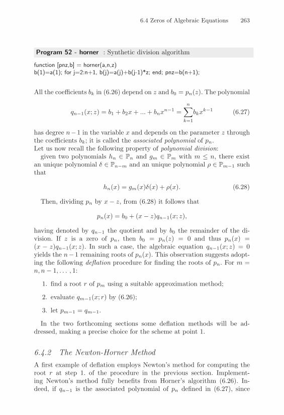
6.4 Zeros of Algebraic Equations 263
Program 52 - horner : Synthetic division algorithm
function [pnz,b] = horner(a,n,z)b(1)=a(1); for j=2:n+1, b(j)=a(j)+b(j-1)*z; end; pnz=b(n+1);
All the coe"cients bk in (6.26) depend on z and b0 = pn(z). The polynomial
qn"1(x; z) = b1 + b2x + ... + bnxn"1 =
n(
k=1
bkxk"1 (6.27)
has degree n"1 in the variable x and depends on the parameter z throughthe coe"cients bk; it is called the associated polynomial of pn.Let us now recall the following property of polynomial division:
given two polynomials hn ! Pn and gm ! Pm with m & n, there existan unique polynomial % ! Pn"m and an unique polynomial ) ! Pm"1 suchthat
hn(x) = gm(x)%(x) + )(x). (6.28)
Then, dividing pn by x" z, from (6.28) it follows that
pn(x) = b0 + (x" z)qn"1(x; z),
having denoted by qn"1 the quotient and by b0 the remainder of the di-vision. If z is a zero of pn, then b0 = pn(z) = 0 and thus pn(x) =(x " z)qn"1(x; z). In such a case, the algebraic equation qn"1(x; z) = 0yields the n" 1 remaining roots of pn(x). This observation suggests adopt-ing the following deflation procedure for finding the roots of pn. For m =n, n" 1, . . . , 1:
1. find a root r of pm using a suitable approximation method;
2. evaluate qm"1(x; r) by (6.26);
3. let pm"1 = qm"1.
In the two forthcoming sections some deflation methods will be ad-dressed, making a precise choice for the scheme at point 1.
6.4.2 The Newton-Horner MethodA first example of deflation employs Newton’s method for computing theroot r at step 1. of the procedure in the previous section. Implement-ing Newton’s method fully benefits from Horner’s algorithm (6.26). In-deed, if qn"1 is the associated polynomial of pn defined in (6.27), since

264 6. Rootfinding for Nonlinear Equations
p*n(x) = qn"1(x; z) + (x" z)q*n"1(x; z) then p*n(z) = qn"1(z; z). Thanks tothis identity, the Newton-Horner method for the approximation of a root(real or complex) rj of pn (j = 1, . . . , n) takes the following form:given an initial estimate r(0)
j of the root, solve for any k ) 0
r(k+1)j = r(k)
j "pn(r(k)
j )
p*n(r(k)j )
= r(k)j "
pn(r(k)j )
qn"1(r(k)j ; r(k)
j ). (6.29)
Once convergence has been achieved for the iteration (6.29), polynomialdeflation is performed, this deflation being helped by the fact that pn(x) =(x " rj)pn"1(x). Then, the approximation of a root of pn"1(x) is carriedout until all the roots of pn have been computed.
Denoting by nk = n" k the degree of the polynomial that is obtained ateach step of the deflation process, for k = 0, . . . , n" 1, the computationalcost of each Newton-Horner iteration (6.29) is equal to 4nk. If rj ! C, itis necessary to work in complex arithmetic and take r(0)
j ! C; otherwise,indeed, the Newton-Horner method (6.29) would yield a sequence {r(k)
j } ofreal numbers.
The deflation procedure might be a!ected by rounding error propagationand, as a consequence, can lead to inaccurate results. For the sake of stabil-ity, it is therefore convenient to approximate first the root r1 of minimummodule, which is the most sensitive to ill-conditioning of the problem (seeExample 2.7, Chapter 2) and then to continue with the successive rootsr2, . . . , until the root of maximum module is computed. To localize r1, thetechniques described in Section 5.1 or the method of Sturm sequences canbe used (see [IK66], p. 126).A further increase in accuracy can be obtained, once an approximation Drjof the root rj is available, by going back to the original polynomial pn andgenerating through the Newton-Horner method (6.29) a new approximationto rj , taking as initial guess r(0)
j = Drj . This combination of deflation andsuccessive correction of the root is called the Newton-Horner method withrefinement.
Example 6.7 Let us examine the performance of the Newton-Horner method intwo cases: in the first one, the polynomial admits real roots, while in the secondone there are two pairs of complex conjugate roots. To single out the importanceof refinement, we have implemented (6.29) both switching it on and o" (methodsNwtRef and Nwt, respectively). The approximate roots obtained using method Nwtare denoted by rj , while sj are those computed by method NwtRef. As for thenumerical experiments, the computations have been done in complex arithmetic,with x(0) = 0+ i 0, i being the imaginary unit, nmax = 100 and toll = 10%5. Thetolerance for the stopping test in the refinement cycle has been set to 10%3toll.
1) p5(x) = x5 + x4 % 9x3 % x2 + 20x% 12 = (x% 1)2(x% 2)(x + 2)(x + 3).
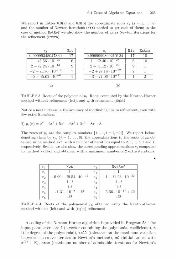
6.4 Zeros of Algebraic Equations 265
We report in Tables 6.3(a) and 6.3(b) the approximate roots rj (j = 1, . . . , 5)and the number of Newton iterations (Nit) needed to get each of them; in thecase of method NwtRef we also show the number of extra Newton iterations forthe refinement (Extra).
rj Nit0.99999348047830 171" i3.56 · 10"25 62" i2.24 · 10"13 9"2" i1.70 · 10"10 7"3 + i5.62 · 10"6 1
(a)
sj Nit Extra0.9999999899210124 17 10
1" i2.40 · 10"28 6 102 + i1.12 · 10"22 9 1"2 + i8.18 · 10"22 7 1"3" i7.06 · 10"21 1 2
(b)
TABLE 6.3. Roots of the polynomial p5. Roots computed by the Newton-Hornermethod without refinement (left), and with refinement (right)
Notice a neat increase in the accuracy of rootfinding due to refinement, even withfew extra iterations.
2) p6(x) = x6 % 2x5 + 5x4 % 6x3 + 2x2 + 8x% 8.
The zeros of p6 are the complex numbers {1,%1, 1 ± i,±2i}. We report below,denoting them by rj , (j = 1, . . . , 6), the approximations to the roots of p6 ob-tained using method Nwt, with a number of iterations equal to 2, 1, 1, 7, 7 and 1,respectively. Beside, we also show the corresponding approximations sj computedby method NwtRef and obtained with a maximum number of 2 extra iterations.
•
rj Nwt sj NwtRefr1 1 s1 1r2 "0.99" i9.54 · 10"17 s2 "1 + i1.23 · 10"32
r3 1+i s3 1+ir4 1-i s4 1-ir5 -1.31 · 10"8 + i2 s5 "5.66 · 10"17 + i2r6 -i2 s6 -i2
TABLE 6.4. Roots of the polynomial p6 obtained using the Newton-Hornermethod without (left) and with (right) refinement
A coding of the Newton-Horner algorithm is provided in Program 53. Theinput parameters are A (a vector containing the polynomial coe"cients), n(the degree of the polynomial), toll (tolerance on the maximum variationbetween successive iterates in Newton’s method), x0 (initial value, withx(0) ! R), nmax (maximum number of admissible iterations for Newton’s

266 6. Rootfinding for Nonlinear Equations
method) and iref (if iref = 1, then the refinement procedure is activated).For dealing with the general case of complex roots, the initial datum isautomatically converted into the complex number z = x(0) + ix(0), wherei =
/"1.
The program returns as output the variables xn (a vector containing thesequence of iterates for each zero of pn(x)), iter (a vector containing thenumber of iterations needed to approximate each root), itrefin (a vectorcontaining the Newton iterations required to refine each estimate of thecomputed root) and root (vector containing the computed roots).
Program 53 - newthorn : Newton-Horner method with refinement
function [xn,iter,root,itrefin]=newthorn(A,n,toll,x0,nmax,iref)apoly=A;for i=1:n, it=1; xn(it,i)=x0+sqrt(-1)*x0; err=toll+1; Ndeg=n-i+1;if (Ndeg == 1), it=it+1; xn(it,i)=-A(2)/A(1);else
while (it < nmax & err > toll),[px,B]=horner(A,Ndeg,xn(it,i));[pdx,C]=horner(B,Ndeg-1,xn(it,i));it=it+1; if (pdx ˜=0), xn(it,i)=xn(it-1,i)-px/pdx;err=max(abs(xn(it,i)-xn(it-1,i)),abs(px));else,
disp(’ Stop due to a vanishing p’’ ’);err=0; xn(it,i)=xn(it-1,i);
endend
endA=B;if (iref==1), alfa=xn(it,i); itr=1; err=toll+1;
while ((err > toll*1e-3) & (itr < nmax))[px,B]=horner(apoly,n,alfa);[pdx,C]=horner(B,n-1,alfa); itr=itr+1;if (pdx˜=0)
alfa2=alfa-px/pdx;err=max(abs(alfa2-alfa),abs(px)); alfa=alfa2;
else,disp(’ Stop due to a vanishing p’’ ’); err=0;
endend; itrefin(i)=itr-1; xn(it,i)=alfa;
enditer(i)=it-1; root(i)=xn(it,i); x0=root(i);
end

6.4 Zeros of Algebraic Equations 267
6.4.3 The Muller MethodA second example of deflation employs Muller’s method for finding anapproximation to the root r at step 1. of the procedure described in Section6.4.1 (see [Mul56]). Unlike Newton’s or secant methods, Muller’s method isable to compute complex zeros of a given function f , even starting from areal initial datum; moreover, its order of convergence is almost quadratic.
The action of Muller’s method is drawn in Figure 6.5. The scheme ex-tends the secant method, substituting the linear polynomial introduced in(6.13) with a second-degree polynomial as follows. Given three distinctvalues x(0), x(1) and x(2), the new point x(3) is determined by settingp2(x(3)) = 0, where p2 ! P2 is the unique polynomial that interpolatesf at the points x(i), i = 0, 1, 2, that is, p2(x(i)) = f(x(i)) for i = 0, 1, 2.Therefore,
x(3)
f
p2
x(0)x(1) x(2)
FIGURE 6.5. The first step of Muller’s method
p2(x) = f(x(2)) + (x% x(2))f [x(2), x(1)] + (x% x(2))(x% x(1))f [x(2), x(1), x(0)]
where
f [*, -] =f(-)" f(*)
- " * , f [*, -, 5 ] =f [-, 5 ]" f [*, -]
5 " *
are the divided di!erences of order 1 and 2 associated with the points *, -and 5 (see Section 8.2.1). Noticing that x"x(1) = (x"x(2))+(x(2)"x(1)),we get
p2(x) = f(x(2)) + w(x" x(2)) + f [x(2), x(1), x(0)](x" x(2))2
having defined
w = f [x(2), x(1)] + (x(2) " x(1))f [x(2), x(1), x(0)]
= f [x(2), x(1)] + f [x(2), x(0)]" f [x(0), x(1)].
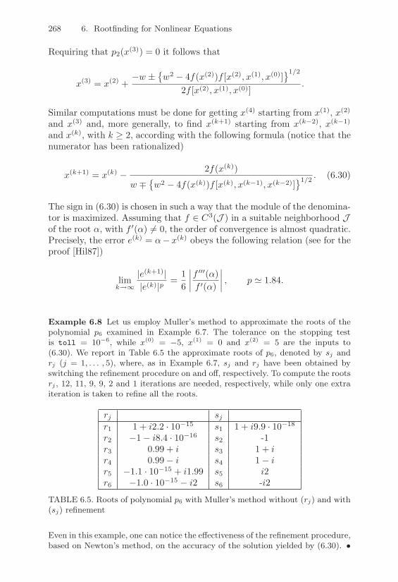
268 6. Rootfinding for Nonlinear Equations
Requiring that p2(x(3)) = 0 it follows that
x(3) = x(2) +"w ±
/w2 " 4f(x(2))f [x(2), x(1), x(0)]
01/2
2f [x(2), x(1), x(0)].
Similar computations must be done for getting x(4) starting from x(1), x(2)
and x(3) and, more generally, to find x(k+1) starting from x(k"2), x(k"1)
and x(k), with k ) 2, according with the following formula (notice that thenumerator has been rationalized)
x(k+1) = x(k) " 2f(x(k))
w </w2 " 4f(x(k))f [x(k), x(k"1), x(k"2)]
01/2 . (6.30)
The sign in (6.30) is chosen in such a way that the module of the denomina-tor is maximized. Assuming that f ! C3(J ) in a suitable neighborhood Jof the root ", with f *(") '= 0, the order of convergence is almost quadratic.Precisely, the error e(k) = "" x(k) obeys the following relation (see for theproof [Hil87])
limk&$
|e(k+1)||e(k)|p
=16
>>>>f ***(")f *(")
>>>> , p 1 1.84.
Example 6.8 Let us employ Muller’s method to approximate the roots of thepolynomial p6 examined in Example 6.7. The tolerance on the stopping testis toll = 10%6, while x(0) = %5, x(1) = 0 and x(2) = 5 are the inputs to(6.30). We report in Table 6.5 the approximate roots of p6, denoted by sj andrj (j = 1, . . . , 5), where, as in Example 6.7, sj and rj have been obtained byswitching the refinement procedure on and o", respectively. To compute the rootsrj , 12, 11, 9, 9, 2 and 1 iterations are needed, respectively, while only one extraiteration is taken to refine all the roots.
rj sjr1 1 + i2.2 · 10"15 s1 1 + i9.9 · 10"18
r2 "1" i8.4 · 10"16 s2 -1r3 0.99 + i s3 1 + ir4 0.99" i s4 1" ir5 "1.1 · 10"15 + i1.99 s5 i2r6 "1.0 · 10"15 " i2 s6 -i2
TABLE 6.5. Roots of polynomial p6 with Muller’s method without (rj) and with(sj) refinement
Even in this example, one can notice the e"ectiveness of the refinement procedure,based on Newton’s method, on the accuracy of the solution yielded by (6.30). •

6.5 Stopping Criteria 269
The Muller method is implemented in Program 54, in the special casewhere f is a polynomial of degree n. The deflation process also includes arefinement phase; the evaluation of f(x(k"2)), f(x(k"1)) and f(x(k)), withk ) 2, is carried out using Program 52. The input/output parameters areanalogous to those described in Program 53.
Program 54 - mulldefl : Muller’s method with refinement
function [xn,iter,root,itrefin]=mulldefl(A,n,toll,x0,x1,x2,nmax,iref)apoly=A;for i=1:nxn(1,i)=x0; xn(2,i)=x1; xn(3,i)=x2; it=0; err=toll+1; k=2; Ndeg=n-i+1;if (Ndeg == 1), it=it+1; k=0; xn(it,i)=-A(2)/A(1);elsewhile ((err > toll) & (it < nmax)),k=k+1; it=it+1; [f0,B]=horner(A,Ndeg,xn(k-2,i));[f1,B]=horner(A,Ndeg,xn(k-1,i)); [f2,B]=horner(A,Ndeg,xn(k,i));f01=(f1-f0)/(xn(k-1,i)-xn(k-2,i)); f12=(f2-f1)/(xn(k,i)-xn(k-1,i));f012=(f12-f01)/(xn(k,i)-xn(k-2,i)); w=f12+(xn(k,i)-xn(k-1,i))*f012;arg=wˆ2-4*f2*f012; d1=w-sqrt(arg); d2=w+sqrt(arg); den=max(d1,d2);if (den˜=0); xn(k+1,i)=xn(k,i)-(2*f2)/den;err=abs(xn(k+1,i)-xn(k,i));
elsedisp(’ Vanishing denominator ’); return; end;
end; end; radix=xn(k+1,i);if (iref==1),alfa=radix; itr=1; err=toll+1;while ((err > toll*1e-3) & (itr < nmax)),[px,B]=horner(apoly,n,alfa); [pdx,C]=horner(B,n-1,alfa);if (pdx == 0), disp(’ Vanishing derivative ’); err=0; end;itr=itr+1; if (pdx˜=0), alfa2=alfa-px/pdx;err=abs(alfa2-alfa); alfa=alfa2; end;end; itrefin(i)=itr-1; xn(k+1,i)=alfa; radix=alfa;
enditer(i)=it; root(i)=radix; [px,B]=horner(A,Ndeg-1,xn(k+1,i)); A=B;end
6.5 Stopping Criteria
Suppose that {x(k)} is a sequence converging to a zero " of the functionf . In this section we provide some stopping criteria for terminating theiterative process that approximates ". Analogous to Section 4.6, wherethe case of iterative methods for linear systems has been examined, thereare two possible criteria: a stopping test based on the residual and on theincrement. Below, + is a fixed tolerance on the approximate calculation of

270 6. Rootfinding for Nonlinear Equations
" and e(k) = ""x(k) denotes the absolute error. We shall moreover assumethat f is continuously di!erentiable in a suitable neighborhood of the root.
1. Control of the residual: the iterative process terminates at the firststep k such that |f(x(k))| < +.
Situations can arise where the test turns out to be either too restrictive orexcessively optimistic (see Figure 6.6). Applying the estimate (6.6) to thecase at hand yields
|e(k)||"| "
4m!
|f (m)(")||"|m
51/m
|f(x(k))|1/m.
In particular, in the case of simple roots, the error is bound to the residualby the factor 1/|f *(")| so that the following conclusions can be drawn:
1. if |f *(")| 1 1, then |e(k)| 1 +; therefore, the test provides a satisfac-tory indication of the error;
2. if |f *(")|: 1, the test is not reliable since |e(k)| could be quite largewith respect to +;
3. if, finally, |f *(")|4 1, we get |e(k)|: + and the test is too restrictive.
We refer to Figure 6.6 for an illustration of the last two cases.
f(x)
x(k)" "
f(x)
x(k)
FIGURE 6.6. Two situations where the stopping test based on the residualis either too restrictive (when |e(k)| 2 |f(x(k))|, left) or too optimistic (when|e(k)|7 |f(x(k))|, right)
The conclusions that we have drawn agree with those in Example 2.4.Indeed, when f *(") 1 0, the condition number of the problem f(x) = 0 isvery high and, as a consequence, the residual does not provide a significantindication of the error.
2. Control of the increment: the iterative process terminates as soon as|x(k+1) " x(k)| < +.
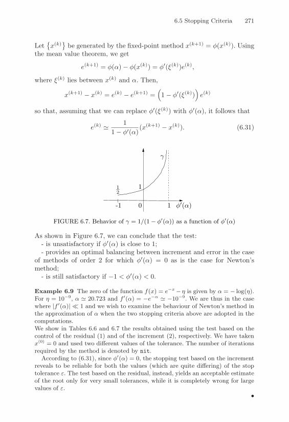
6.5 Stopping Criteria 271
Let/x(k)0 be generated by the fixed-point method x(k+1) = 4(x(k)). Using
the mean value theorem, we get
e(k+1) = 4(")" 4(x(k)) = 4*(*(k))e(k),
where *(k) lies between x(k) and ". Then,
x(k+1) " x(k) = e(k) " e(k+1) =K1" 4*(*(k))
Le(k)
so that, assuming that we can replace 4*(*(k)) with 4*("), it follows that
e(k) 1 11" 4*(")
(x(k+1) " x(k)). (6.31)
-1 1 4*(")0
112
'
FIGURE 6.7. Behavior of , = 1/(1% 3(($)) as a function of 3(($)
As shown in Figure 6.7, we can conclude that the test:- is unsatisfactory if 4*(") is close to 1;- provides an optimal balancing between increment and error in the case
of methods of order 2 for which 4*(") = 0 as is the case for Newton’smethod;
- is still satisfactory if "1 < 4*(") < 0.
Example 6.9 The zero of the function f(x) = e%x% 0 is given by $ = % log(0).For 0 = 10%9, $ 0 20.723 and f (($) = %e%! 0 %10%9. We are thus in the casewhere |f (($)|2 1 and we wish to examine the behaviour of Newton’s method inthe approximation of $ when the two stopping criteria above are adopted in thecomputations.We show in Tables 6.6 and 6.7 the results obtained using the test based on thecontrol of the residual (1) and of the increment (2), respectively. We have takenx(0) = 0 and used two di"erent values of the tolerance. The number of iterationsrequired by the method is denoted by nit.
According to (6.31), since 3(($) = 0, the stopping test based on the incrementreveals to be reliable for both the values (which are quite di"ering) of the stoptolerance &. The test based on the residual, instead, yields an acceptable estimateof the root only for very small tolerances, while it is completely wrong for largevalues of &.
•
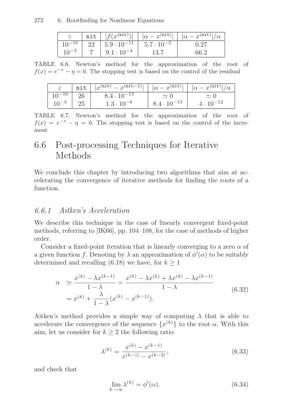
272 6. Rootfinding for Nonlinear Equations
+ nit |f(x(nit))| |"" x(nit)| |"" x(nit)|/"10"10 22 5.9 · 10"11 5.7 · 10"2 0.2710"3 7 9.1 · 10"4 13.7 66.2
TABLE 6.6. Newton’s method for the approximation of the root off(x) = e%x % 0 = 0. The stopping test is based on the control of the residual
+ nit |x(nit) " x(nit"1)| |"" x(nit)| |"" x(nit)|/"10"10 26 8.4 · 10"13 1 0 1 010"3 25 1.3 · 10"6 8.4 · 10"13 4 · 10"12
TABLE 6.7. Newton’s method for the approximation of the root off(x) = e%x % 0 = 0. The stopping test is based on the control of the incre-ment
6.6 Post-processing Techniques for IterativeMethods
We conclude this chapter by introducing two algorithms that aim at ac-celerating the convergence of iterative methods for finding the roots of afunction.
6.6.1 Aitken’s AccelerationWe describe this technique in the case of linearly convergent fixed-pointmethods, referring to [IK66], pp. 104–108, for the case of methods of higherorder.
Consider a fixed-point iteration that is linearly converging to a zero " ofa given function f . Denoting by $ an approximation of 4*(") to be suitablydetermined and recalling (6.18) we have, for k ) 1
" 1 x(k) " $x(k"1)
1" $ =x(k) " $x(k) + $x(k) " $x(k"1)
1" $
= x(k) +$
1" $ (x(k) " x(k"1)).(6.32)
Aitken’s method provides a simple way of computing $ that is able toaccelerate the convergence of the sequence {x(k)} to the root ". With thisaim, let us consider for k ) 2 the following ratio
$(k) =x(k) " x(k"1)
x(k"1) " x(k"2) , (6.33)
and check that
limk&$
$(k) = 4*("). (6.34)

6.6 Post-processing Techniques for Iterative Methods 273
Indeed, for k su"ciently large
x(k+2) " " 1 4*(")(x(k+1) " ")
and thus, elaborating (6.33), we get
limk&$
$(k) = limk&$
x(k) " x(k"1)
x(k"1) " x(k"2) = limk&$
(x(k) " ")" (x(k"1) " ")(x(k"1) " ")" (x(k"2) " ")
= limk&$
x(k) " "x(k"1) " "
" 1
1" x(k"2) " "x(k"1) " "
=4*(")" 1
1" 14*(")
= 4*(")
which is (6.34). Substituting in (6.32) $ with its approximation $(k) givenby (6.33), yields the updated estimate of "
" 1 x(k) +$(k)
1" $(k) (x(k) " x(k"1)) (6.35)
which, rigorously speaking, is significant only for a su"ciently large k.However, assuming that (6.35) holds for any k ) 2, we denote by :x(k) thenew approximation of " that is obtained by plugging (6.33) back into (6.35)
:x(k) = x(k) " (x(k) " x(k"1))2
(x(k) " x(k"1))" (x(k"1) " x(k"2)), k ) 2. (6.36)
This relation is known as Aitken’s extrapolation formula.Letting, for k ) 2,
=x(k) = x(k) " x(k"1), =2x(k) = =(=x(k)) = =x(k+1) "=x(k),
formula (6.36) can be written as
:x(k) = x(k) " (=x(k))2
=2x(k"1) , k ) 2. (6.37)
Form (6.37) explains the reason why method (6.36) is more commonlyknown as Aitken’s =2 method.For the convergence analysis of Aitken’s method, it is useful to write (6.36)as a fixed-point method in the form (6.17), by introducing the iterationfunction
4.(x) =x4(4(x))" 42(x)4(4(x))" 24(x) + x
. (6.38)
This function is indeterminate at x = " since 4(") = "; however, byapplying L’Hospital’s rule one can easily check that limx&! 4.(x) = "

274 6. Rootfinding for Nonlinear Equations
under the assumption that 4 is di!erentiable at " and 4*(") '= 1. Thus, 4.is consistent and has a continuos extension at ", the same being also trueif " is a multiple root of f . Moreover, it can be shown that the fixed pointsof (6.38) coincide with those of 4 even in the case where " is a multipleroot of f (see [IK66], pp. 104-106).
From (6.38) we conclude that Aitken’s method can be applied to a fixed-point method x = 4(x) of arbitrary order. Actually, the following conver-gence result holds.
Property 6.7 (convergence of Aitken’s method) Let x(k+1) = 4(x(k))be a fixed-point iteration of order p ) 1 for the approximation of a simplezero " of a function f . If p = 1, Aitken’s method converges to " with order2, while if p ) 2 the convergence order is 2p " 1. In particular, if p = 1,Aitken’s method is convergent even if the fixed-point method is not. If "has multiplicity m ) 2 and the method x(k+1) = 4(x(k)) is first-order con-vergent, then Aitken’s method converges linearly, with convergence factorC = 1" 1/m.
Example 6.10 Consider the computation of the simple zero $ = 1 for the func-tion f(x) = (x% 1)ex. For this, we use three fixed-point methods whose iterationfunctions are, respectively, 30(x) = log(xex), 31(x) = (ex + x)/(ex + 1) and32(x) = (x2 % x + 1)/x (for x $= 0). Notice that, since |3(
0(1)| = 2, the corre-sponding fixed-point method is not convergent, while in the other two cases themethods have order 1 and 2, respectively.
Let us check the performance of Aitken’s method, running Program 55 withx(0) = 2, toll = 10%10 and working in complex arithmetic. Notice that in the caseof 30 this produces complex numbers if x(k) happens to be negative. Accordingto Property 6.7, Aitken’s method applied to the iteration function 30 convergesin 8 steps to the value x(8) = 1.000002 + i 0.000002. In the other two cases, themethod of order 1 converges to $ in 18 iterations, to be compared with the 4iterations required by Aitken’s method, while in the case of the iteration function32 convergence holds in 7 iterations against 5 iterations required by Aitken’smethod. •
Aitken’s method is implemented in Program 55. The input/output pa-rameters are the same as those of previous programs in this chapter.
Program 55 - aitken : Aitken’s extrapolation
function [xvect,xdif,fx,nit]=aitken(x0,nmax,toll,phi,fun)nit=0; xvect=[x0]; x=x0; fxn=eval(fun);fx=[fxn]; xdif=[]; err=toll+1;while err >= toll & nit <= nmaxnit=nit+1; xv=xvect(nit); x=xv; phix=eval(phi);x=phix; phixx=eval(phi); den=phixx-2*phix+xv;if den == 0, err=toll*1.e-01;else, xn=(xv*phixx-phixˆ2)/den; xvect=[xvect; xn];
xdif=[xdif; abs(xn-xv)]; x=xn; fxn=abs(eval(fun));

6.6 Post-processing Techniques for Iterative Methods 275
fx=[fx; fxn]; err=fxn;end
end
6.6.2 Techniques for Multiple RootsAs previously noticed in deriving Aitken’s acceleration, taking the incre-mental ratios of successive iterates $(k) in (6.33) provides a way to estimatethe asymptotic convergence factor 4*(").
This information can be employed also to estimate the multiplicity of theroot of a nonlinear equation and, as a consequence, it provides a tool formodifying Newton’s method in order to recover its quadratic convergence(see (6.23)). Indeed, define the sequence m(k) through the relation $(k) =1" 1/m(k), and recalling (6.22), it follows that m(k) tends to m as k (,.If the multiplicity m is known a priori, it is clearly convenient to use themodified Newton method (6.23). In other cases, the following adaptive New-ton algorithm can be used
x(k+1) = x(k) "m(k) f(x(k))f *(x(k))
, k ) 2, (6.39)
where we have set
m(k) =1
1" $(k) =x(k"1) " x(k"2)
2x(k"1) " x(k) " x(k"2) . (6.40)
Example 6.11 Let us check the performances of Newton’s method in its threeversions proposed so far (standard (6.16), modified (6.23) and adaptive (6.39)),to approximate the multiple zero $ = 1 of the function f(x) = (x2 % 1)p log x(for p ! 1 and x > 0). The desired root has multiplicity m = p + 1. The valuesp = 2, 4, 6 have been considered and x(0) = 0.8, toll=10%10 have always beentaken in numerical computations.
The obtained results are summarized in Table 6.8, where for each methodthe number of iterations nit required to converge are reported. In the case ofthe adaptive method, beside the value of nit we have also shown in braces theestimate m(nit) of the multiplicity m that is yielded by Program 56. •
m standard adaptive modified3 51 13 (2.9860) 45 90 16 (4.9143) 57 127 18 (6.7792) 5
TABLE 6.8. Solution of problem (x2%1)p log x = 0 in the interval [0.5, 1.5], withp = 2, 4, 6

276 6. Rootfinding for Nonlinear Equations
In Example 6.11, the adaptive Newton method converges more rapidlythan the standard method, but less rapidly than the modified Newtonmethod. It must be noticed, however, that the adaptive method yields asa useful by-product a good estimate of the multiplicity of the root, whichcan be profitably employed in a deflation procedure for the approximationof the roots of a polynomial.
The algorithm 6.39, with the adaptive estimate (6.40) of the multiplicityof the root, is implemented in Program 56. To avoid the onset of numericalinstabilities, the updating of m(k) is performed only when the variation be-tween two consecutive iterates is su"ciently diminished. The input/outputparameters are the same as those of previous programs in this chapter.
Program 56 - adptnewt : Adaptive Newton’s method
function [xvect,xdif,fx,nit,m] = adptnewt(x0,nmax,toll,fun,dfun)xvect=x0; nit=0; r=[1]; err=toll+1; m=[1]; xdif=[];while (nit < nmax) & (err > toll)
nit=nit+1; x=xvect(nit); fx(nit)=eval(fun); f1x=eval(dfun);if (f1x == 0), disp(’ Stop due to vanishing derivative ’); return; end;x=x-m(nit)*fx(nit)/f1x; xvect=[xvect;x]; fx=[fx;eval(fun)];rd=err; err=abs(xvect(nit+1)-xvect(nit)); xdif=[xdif;err];ra=err/rd; r=[r;ra]; di!=abs(r(nit+1)-r(nit));if (di! < 1.e-3) & (r(nit+1) > 1.e-2),
m(nit+1)=max(m(nit),1/abs(1-r(nit+1)));else, m(nit+1)=m(nit); end
end
6.7 Applications
We apply iterative methods for nonlinear equations considered so far in thesolution of two problems arising in the study of the thermal properties ofgases and electronics, respectively.
6.7.1 Analysis of the State Equation for a Real GasFor a mole of a perfect gas, the state equation Pv = RT establishes a re-lation between the pressure P of the gas (in Pascals [Pa]), the specific vol-ume v (in cubic meters per kilogram [m3Kg"1]) and its temperature T (inKelvin [K]), R being the universal gas constant, expressed in [JKg"1K"1](joules per kilogram per Kelvin).
For a real gas, the deviation from the state equation of perfect gases isdue to van der Waals and takes into account the intermolecular interactionand the space occupied by molecules of finite size (see [Sla63]).

6.7 Applications 277
Denoting by " and # the gas constants according to the van der Waalsmodel, in order to determine the specific volume v of the gas, once P andT are known, we must solve the nonlinear equation
f(v) = (P + "/v2)(v " #)"RT = 0. (6.41)
With this aim, let us consider Newton’s method (6.16) in the case of carbondioxide (CO2), at the pressure of P = 10[atm] (equal to 1013250[Pa]) andat the temperature of T = 300[K]. In such a case, " = 188.33[Pam6Kg"2]and # = 9.77 · 10"4[m3Kg"1]; as a comparison, the solution computed byassuming that the gas is perfect is v 1 0.056[m3Kg"1].
We report in Table 6.9 the results obtained by running Program 50 fordi!erent choices of the initial guess v(0). We have denoted by Nit the num-ber of iterations needed by Newton’s method to converge to the root v, off(v) = 0 using an absolute tolerance equal to the roundo! unit.
v(0) Nit v(0) Nit v(0) Nit v(0) Nit
10"4 47 10"2 7 10"3 21 10"1 5
TABLE 6.9. Convergence of Newton’s method to the root of equation (6.41)
The computed approximation of v, is vNit 1 0.0535. To analyze the causesof the strong dependence of Nit on the value of v(0), let us examine thederivative f *(v) = P " "v"2 + 2"#v"3. For v > 0, f *(v) = 0 at vM 11.99 ·10"3[m3Kg"1] (relative maximum) and at vm 1 1.25 ·10"2[m3Kg"1](relative minimum), as can be seen in the graph of Figure 6.8 (left).A choice of v(0) in the interval (0, vm) (with v(0) '= vM ) thus necessarilyleads to a slow convergence of Newton’s method, as demonstrated in Figure6.8 (right), where, in solid circled line, the sequence {|v(k+1) " v(k)|} isshown, for k ) 0.
A possible remedy consists of resorting to a polyalgorithmic approach,based on the sequential use of the bisection method and Newton’s method(see Section 6.2.1). Running the bisection-Newton’s method with the end-points of the search interval equal to a = 10"4[m3Kg"1] and b = 0.1[m3Kg"1]and an absolute tolerance of 10"3[m3Kg"1], yields an overall convergenceof the algorithm to the root v, in 11 iterations, with an accuracy of theorder of the roundo! unit. The plot of the sequence {|v(k+1) " v(k)|}, fork ) 0, is shown in solid and starred lines in Figure 6.8 (right).
6.7.2 Analysis of a Nonlinear Electrical CircuitLet us consider the electrical circuit in Figure 6.9 (left), where v and jdenote respectively the voltage drop across the device D (called a tunnelingdiode) and the current flowing through D, while R and E are a resistor anda voltage generator of given values.

278 6. Rootfinding for Nonlinear Equations
0 0.02 0.04 0.06 0.08 0.1!6
!4
!2
0
2
4
6x 10
4
0 10 20 30 40 5010
!18
10!16
10!14
10!12
10!10
10!8
10!6
10!4
10!2
100
FIGURE 6.8. Graph of the function f in (6.41) (left); increments |v(k+1) % v(k)|computed by the Newton’s method (circled curve) and bisection-Newton’smethod (starred curve)
The circuit is commonly employed as a biasing circuit for electronic de-vices working at high frequency (see [Col66]). In such applications the pa-rameters R and E are designed in such a way that v attains a value internalto the interval for which g*(v) < 0, where g is the function which describesthe bound between current and voltage for D and is drawn in Figure 6.9(right). Explicitly, g = "(ev/' " 1)"µv(v" '), for suitable constants ", #,' and µ.
_+
j
E
RD v
0 0.1 0.2 0.3 0.4 0.5!4
!2
0
2
4
6
8
10
12x 10
!5
g(v)
FIGURE 6.9. Tunneling diode circuit (left) and working point computation(right)
Our aim is to determine the working point of the circuit at hand, thatis, the values attained by v and j for given parameters R and E. For that,we write Kirchho!’s law for the voltages across the loop, obtaining thefollowing nonlinear equation
f(v) = v
41R
+ µ'
5" µv2 + "(ev/' " 1)" E
R= 0. (6.42)
From a graphical standpoint, finding out the working point of the circuitamounts to determining the intersection between the function g and the

6.8 Exercises 279
straight line of equation j = (E " v)/R, as shown in Figure 6.9 (right).Assume the following (real-life) values for the parameters of the problem:E/R = 1.2·10"4 [A], " = 10"12 [A], #"1 = 40 [V "1], µ = 10"3 [AV "2] and' = 0.4 [V ]. The solution of (6.42), which is also unique for the consideredvalues of the parameters, is v, 1 0.3 [V ].
To approximate v,, we compare the main iterative methods introducedin this chapter. We have taken v(0) = 0 [V ] for Newton’s method, * = 0for the Dekker-Brent algorithm (for the meaning of *, see Example 6.5),while for all the other schemes the search interval has been taken equal to[0, 0.5]. The stopping tolerance toll has been set to 10"10. The obtainedresults are reported in Table 6.10 where nit and f (nit) denote respectivelythe number of iterations needed by the method to converge and the valueof f at the computed solution.
Notice the extremely slow convergence of the Regula Falsi method, dueto the fact that the value v(k%) always coincides with the right end-pointv = 0.5 and the function f around v, has derivative very close to zero. Ananalogous interpretation holds for the chord method.
Method nit f (nit) Method nit f (nit)
bisection 33 "1.12 · 10"15 Dekker-Brent 11 1.09 · 10"14
Regula Falsi 225 "9.77 · 10"11 secant 11 2.7 · 10"20
chord 186 "9.80 · 10"14 Newton’s 8 "1.35 · 10"20
TABLE 6.10. Convergence of the methods for the approximation of the root ofequation (6.42)
6.8 Exercises1. Derive geometrically the sequence of the first iterates computed by bisec-
tion, Regula Falsi, secant and Newton’s methods in the approximation ofthe zero of the function f(x) = x2 % 2 in the interval [1, 3].
2. Let f be a continuous function that is m-times di"erentiable (m ! 1), suchthat f($) = . . . = f (m%1)($) = 0 and f (m)($) $= 0. Prove (6.22) and checkthat the modified Newton method (6.23) has order of convergence equal to2.[Hint: let f(x) = (x% $)mh(x), h being a function such that h($) $= 0].
3. Let f(x) = cos2(2x) % x2 be the function in the interval 0 " x " 1.5examined in Example 6.4. Having fixed a tolerance & = 10%10 on the abso-lute error, determine experimentally the subintervals for which Newton’smethod is convergent to the zero $ 0 0.5149.[Solution: for 0 < x(0) " 0.02, 0.94 " x(0) " 1.13 and 1.476 " x(0) " 1.5,the method converges to the solution %$. For any other value of x(0) in[0, 1.5], the method converges to $].
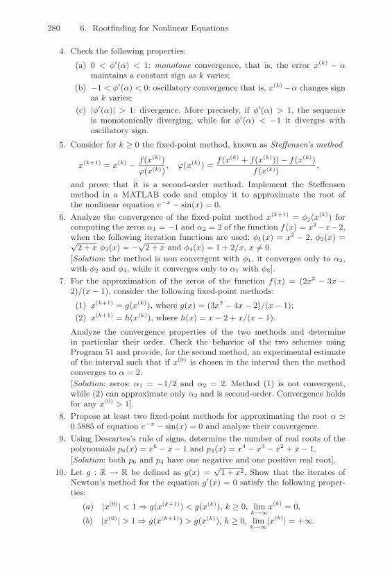
280 6. Rootfinding for Nonlinear Equations
4. Check the following properties:
(a) 0 < 3(($) < 1: monotone convergence, that is, the error x(k) % $maintains a constant sign as k varies;
(b) %1 < 3(($) < 0: oscillatory convergence that is, x(k)%$ changes signas k varies;
(c) |3(($)| > 1: divergence. More precisely, if 3(($) > 1, the sequenceis monotonically diverging, while for 3(($) < %1 it diverges withoscillatory sign.
5. Consider for k ! 0 the fixed-point method, known as Ste!ensen’s method
x(k+1) = x(k) % f(x(k))((x(k))
, ((x(k)) =f(x(k) + f(x(k)))% f(x(k))
f(x(k)),
and prove that it is a second-order method. Implement the Ste"ensenmethod in a MATLAB code and employ it to approximate the root ofthe nonlinear equation e%x % sin(x) = 0.
6. Analyze the convergence of the fixed-point method x(k+1) = 3j(x(k)) forcomputing the zeros $1 = %1 and $2 = 2 of the function f(x) = x2%x%2,when the following iteration functions are used: 31(x) = x2 % 2, 32(x) ='
2 + x 33(x) = %'
2 + x and 34(x) = 1 + 2/x, x $= 0.[Solution: the method is non convergent with 31, it converges only to $2,with 32 and 34, while it converges only to $1 with 33].
7. For the approximation of the zeros of the function f(x) = (2x2 % 3x %2)/(x% 1), consider the following fixed-point methods:
(1) x(k+1) = g(x(k)), where g(x) = (3x2 % 4x% 2)/(x% 1);(2) x(k+1) = h(x(k)), where h(x) = x% 2 + x/(x% 1).
Analyze the convergence properties of the two methods and determinein particular their order. Check the behavior of the two schemes usingProgram 51 and provide, for the second method, an experimental estimateof the interval such that if x(0) is chosen in the interval then the methodconverges to $ = 2.[Solution: zeros: $1 = %1/2 and $2 = 2. Method (1) is not convergent,while (2) can approximate only $2 and is second-order. Convergence holdsfor any x(0) > 1].
8. Propose at least two fixed-point methods for approximating the root $ 00.5885 of equation e%x % sin(x) = 0 and analyze their convergence.
9. Using Descartes’s rule of signs, determine the number of real roots of thepolynomials p6(x) = x6 % x% 1 and p4(x) = x4 % x3 % x2 + x% 1.[Solution: both p6 and p4 have one negative and one positive real root].
10. Let g : R , R be defined as g(x) ='
1 + x2. Show that the iterates ofNewton’s method for the equation g((x) = 0 satisfy the following proper-ties:
(a) |x(0)| < 1 * g(x(k+1)) < g(x(k)), k ! 0, limk$!
x(k) = 0,
(b) |x(0)| > 1 * g(x(k+1)) > g(x(k)), k ! 0, limk$!
|x(k)| = +#.

7Nonlinear Systems and NumericalOptimization
In this chapter we address the numerical solution of systems of nonlinearequations and the minimization of a function of several variables.
The first problem generalizes to the n-dimensional case the search forthe zeros of a function, which was considered in Chapter 6, and can beformulated as follows: given F : Rn ( Rn,
find x, ! Rn such that F(x,) = 0. (7.1)
Problem (7.1) will be solved by extending to several dimensions some ofthe schemes that have been proposed in Chapter 6.The basic formulation of the second problem reads: given f : Rn ( R,called an objective function,
minimize f(x) in Rn, (7.2)
and is called an unconstrained optimization problem.A typical example consists of determining the optimal allocation of n
resources, x1, x2, . . . , xn, in competition with each other and ruled by aspecific law. Generally, such resources are not unlimited; this circumstance,from a mathematical standpoint, amounts to requiring that the minimizerof the objective function lies within a subset ( * Rn, and, possibly, thatsome equality or inequality constraints must be satisfied.
When these constraints exist the optimization problem is called con-strained and can be formulated as follows: given the objective function f ,
minimize f(x) in ( * Rn. (7.3)

282 7. Nonlinear Systems and Numerical Optimization
Remarkable instances of (7.3) are those in which ( is characterized by con-ditions like h(x) = 0 (equality constraints) or h(x) & 0 (inequality con-straints), where h : Rn ( Rm, with m & n, is a given function, called costfunction, and the condition h(x) & 0 means hi(x) & 0, for i = 1, . . . ,m.
If the function h is continuous and ( is connected, problem (7.3) isusually referred to as a nonlinear programming problem. Notable examplesin this area are:
convex programming if f is a convex function and h has convex compo-nents (see (7.21));
linear programming if f and h are linear;
quadratic programming if f is quadratic and h is linear.
Problems (7.1) and (7.2) are strictly related to one another. Indeed, if wedenote by Fi the components of F, then a point x,, a solution of (7.1),is a minimizer of the function f(x) =
!ni=1 F
2i (x). Conversely, assuming
that f is di!erentiable and setting the partial derivatives of f equal tozero at a point x, at which f is minimum leads to a system of nonlinearequations. Thus, any system of nonlinear equations can be associated witha suitable minimization problem, and vice versa. We shall take advantageof this observation when devising e"cient numerical methods.
7.1 Solution of Systems of Nonlinear Equations
Before considering problem (7.1), let us set some notation which will beused throughout the chapter.
For k ) 0, we denote by Ck(D) the set of k-continuously di!erentiablefunctions from D to Rn, where D 7 Rn is a set that will be made precisefrom time to time. We shall always assume that F ! C1(D), i.e., F : Rn (Rn is a continuously di!erentiable function on D.
We denote also by JF(x) the Jacobian matrix associated with F andevaluated at the point x = (x1, . . . , xn)T of Rn, defined as
(JF(x))ij =4.Fi
.xj
5(x), i, j = 1, . . . , n.
Given any vector norm + ·+, we shall henceforth denote the sphere of radiusR with center x, by
B(x,;R) = {y ! Rn : +y " x,+ < R} .

7.1 Solution of Systems of Nonlinear Equations 283
7.1.1 Newton’s Method and Its VariantsAn immediate extension to the vector case of Newton’s method (6.16) forscalar equations can be formulated as follows:
given x(0) ! Rn, for k = 0, 1, . . . , until convergence:
solve JF(x(k))"x(k) = "F(x(k));
set x(k+1) = x(k) + "x(k).(7.4)
Thus, at each step k the solution of a linear system with matrix JF(x(k))is required.
Example 7.1 Consider the nonlinear system)+
,ex
21+x2
2 % 1 = 0,
ex21%x2
2 % 1 = 0,
which admits the unique solution x) = 0. In this case, F(x) = (ex21+x2
2 %1, ex
21%x2
2 % 1). Running Program 57, leads to convergence in 15 iterations to thepair (0.61 · 10%5, 0.61 · 10%5)T , starting from the initial datum x(0) = (0.1, 0.1)T ,thus demonstrating a fairly rapid convergence rate. The results, however, dra-matically change as the choice of the initial guess is varied. For instance, pickingup x(0) = (10, 10)T , 220 iterations are needed to obtain a solution comparable tothe previous one, while, starting from x(0) = (20, 20)T , Newton’s method fails toconverge. •
The previous example points out the high sensitivity of Newton’s methodon the choice of the initial datum x(0), as confirmed by the following localconvergence result.
Theorem 7.1 Let F : Rn ( Rn be a C1 function in a convex open setD of Rn that contains x,. Suppose that J"1
F (x,) exists and that there existpositive constants R, C and L, such that +J"1
F (x,)+ & C and
+JF(x)" JF(y)+ & L+x" y+ #x,y ! B(x,;R),
having denoted by the same symbol + · + two consistent vector and matrixnorms. Then, there exists r > 0 such that, for any x(0) ! B(x,; r), thesequence (7.4) is uniquely defined and converges to x, with
+x(k+1) " x,+ & CL+x(k) " x,+2. (7.5)
Proof. Proceeding by induction on k, let us check (7.5) and, moreover, thatx(k+1) / B(x); r), where r = min(R, 1/(2CL)). First, we prove that for anyx(0) / B(x); r), the inverse matrix J%1
F (x(0)) exists. Indeed
&J%1F (x))[JF(x(0))% JF(x))]& " &J%1
F (x))& &JF(x(0))% JF(x))& " CLr " 12,

284 7. Nonlinear Systems and Numerical Optimization
and thus, thanks to Theorem 1.5, we can conclude that J%1F (x(0)) exists, since
&J%1F (x(0))& " &J%1
F (x))&1% &J%1
F (x))[JF(x(0))% JF(x))]&" 2&J%1
F (x))& " 2C.
As a consequence, x(1) is well defined and
x(1) % x) = x(0) % x) % J%1F (x(0))[F(x(0))% F(x))].
Factoring out J%1F (x(0)) on the right hand side and passing to the norms, we get
&x(1) % x)& " &J%1F (x(0))& &F(x))% F(x(0))% JF(x(0))[x) % x(0)]&
" 2CL2&x) % x(0)&2
where the remainder of Taylor’s series of F has been used. The previous relationproves (7.5) in the case k = 0; moreover, since x(0) / B(x); r), we have &x) %x(0)& " 1/(2CL), from which &x(1) % x)& " 1
2&x) % x(0)&.
This ensures that x(1) / B(x); r).By a similar proof, one can check that, should (7.5) be true for a certain k,
then the same inequality would follow also for k + 1 in place of k. This provesthe theorem. !
Theorem 7.1 thus confirms that Newton’s method is quadratically conver-gent only if x(0) is su"ciently close to the solution x, and if the Jacobianmatrix is nonsingular. Moreover, it is worth noting that the computationale!ort needed to solve the linear system (7.4) can be excessively high as ngets large. Also, JF(x(k)) could be ill-conditioned, which makes it quite di"-cult to obtain an accurate solution. For these reasons, several modificationsto Newton’s method have been proposed, which will be briefly consideredin the later sections, referring to the specialized literature for further details(see [OR70], [DS83], [Erh97], [BS90] and the references therein).
7.1.2 Modified Newton’s MethodsSeveral modifications of Newton’s method have been proposed in orderto reduce its cost when the computed solution is su"ciently close to x,.Further variants, that are globally convergent, will be introduced for thesolution of the minimization problem (7.2).
1. Cyclic updating of the Jacobian matrixAn e"cient alternative to method (7.4) consists of keeping the Jacobian
matrix (more precisely, its factorization) unchanged for a certain number,say p ) 2, of steps. Generally, a deterioration of convergence rate is accom-panied by a gain in computational e"ciency.
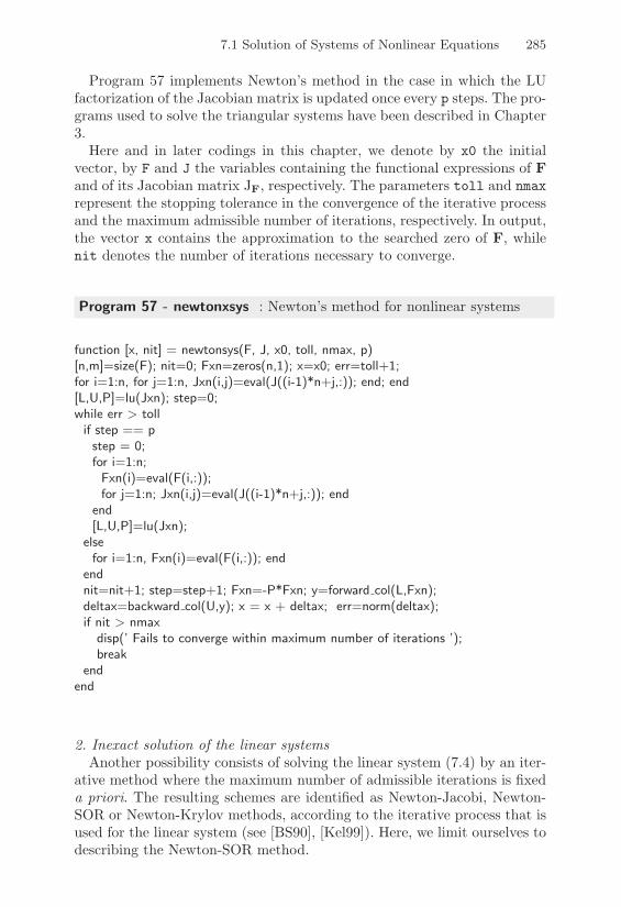
7.1 Solution of Systems of Nonlinear Equations 285
Program 57 implements Newton’s method in the case in which the LUfactorization of the Jacobian matrix is updated once every p steps. The pro-grams used to solve the triangular systems have been described in Chapter3.
Here and in later codings in this chapter, we denote by x0 the initialvector, by F and J the variables containing the functional expressions of Fand of its Jacobian matrix JF, respectively. The parameters toll and nmaxrepresent the stopping tolerance in the convergence of the iterative processand the maximum admissible number of iterations, respectively. In output,the vector x contains the approximation to the searched zero of F, whilenit denotes the number of iterations necessary to converge.
Program 57 - newtonxsys : Newton’s method for nonlinear systems
function [x, nit] = newtonsys(F, J, x0, toll, nmax, p)[n,m]=size(F); nit=0; Fxn=zeros(n,1); x=x0; err=toll+1;for i=1:n, for j=1:n, Jxn(i,j)=eval(J((i-1)*n+j,:)); end; end[L,U,P]=lu(Jxn); step=0;while err > tollif step == pstep = 0;for i=1:n;Fxn(i)=eval(F(i,:));for j=1:n; Jxn(i,j)=eval(J((i-1)*n+j,:)); end
end[L,U,P]=lu(Jxn);
elsefor i=1:n, Fxn(i)=eval(F(i,:)); end
endnit=nit+1; step=step+1; Fxn=-P*Fxn; y=forward col(L,Fxn);deltax=backward col(U,y); x = x + deltax; err=norm(deltax);if nit > nmax
disp(’ Fails to converge within maximum number of iterations ’);break
endend
2. Inexact solution of the linear systemsAnother possibility consists of solving the linear system (7.4) by an iter-
ative method where the maximum number of admissible iterations is fixeda priori. The resulting schemes are identified as Newton-Jacobi, Newton-SOR or Newton-Krylov methods, according to the iterative process that isused for the linear system (see [BS90], [Kel99]). Here, we limit ourselves todescribing the Newton-SOR method.

286 7. Nonlinear Systems and Numerical Optimization
In analogy with what was done in Section 4.2.1, let us decompose theJacobian matrix at step k as
JF(x(k)) = Dk " Ek " Fk (7.6)
where Dk = D(x(k)), "Ek = "E(x(k)) and "Fk = "F(x(k)), the diagonalpart and the lower and upper triangular portions of the matrix JF(x(k)),respectively. We suppose also that Dk is nonsingular. The SOR method forsolving the linear system in (7.4) is organized as follows: setting "x(k)
0 = 0,solve
"x(k)r = Mk"x
(k)r"1 " 0k(Dk " 0kEk)"1F(x(k)), r = 1, 2, . . . , (7.7)
where Mk is the iteration matrix of SOR method
Mk = [Dk " 0kEk]"1 [(1" 0k)Dk + 0kFk] ,
and 0k is a positive relaxation parameter whose optimal value can rarelybe determined a priori. Assume that only r = m steps of the method arecarried out. Recalling that "x(k)
r = x(k)r " x(k) and still denoting by x(k+1)
the approximate solution computed after m steps, we find that this lattercan be written as (see Exercise 1)
x(k+1) = x(k) " 0k
8Mm"1
k + · · · + I9(Dk " 0kEk)
"1 F(x(k)). (7.8)
This method is thus a composite iteration, in which at each step k, startingfrom x(k), m steps of the SOR method are carried out to solve approxi-mately system (7.4).
The integer m, as well as 0k, can depend on the iteration index k; thesimplest choice amounts to performing, at each Newton’s step, only oneiteration of the SOR method, thus obtaining for r = 1 from (7.7) the one-step Newton-SOR method
x(k+1) = x(k) " 0k (Dk " 0kEk)"1 F(x(k)).
In a similar way, the preconditioned Newton-Richardson method with ma-trix Pk, if truncated at the m-th iteration, is
x(k+1) = x(k) "PI + Mk + . . . + Mm"1
k
QP"1k F(x(k)),
where Pk is the preconditioner of JF and
Mk = P"1k Nk, Nk = Pk " JF(x(k)).
For an e"cient implementation of these techniques we refer to the MAT-LAB software package developed in [Kel99].
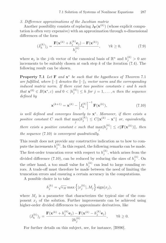
7.1 Solution of Systems of Nonlinear Equations 287
3. Di!erence approximations of the Jacobian matrixAnother possibility consists of replacing JF(x(k)) (whose explicit compu-
tation is often very expensive) with an approximation through n-dimensionaldi!erences of the form
(J(k)h )j =
F(x(k) + h(k)j ej)" F(x(k))
h(k)j
, #k ) 0, (7.9)
where ej is the j-th vector of the canonical basis of Rn and h(k)j > 0 are
increments to be suitably chosen at each step k of the iteration (7.4). Thefollowing result can be shown.
Property 7.1 Let F and x, be such that the hypotheses of Theorem 7.1are fulfilled, where + ·+ denotes the + ·+1 vector norm and the correspondinginduced matrix norm. If there exist two positive constants + and h suchthat x(0) ! B(x,, +) and 0 < |h(k)
j | & h for j = 1, . . . , n then the sequencedefined by
x(k+1) = x(k) "VJ(k)h
W"1F(x(k)), (7.10)
is well defined and converges linearly to x,. Moreover, if there exists apositive constant C such that max
j|h(k)
j | & C+x(k) " x,+ or, equivalently,
there exists a positive constant c such that maxj
|h(k)j | & c+F(x(k))+, then
the sequence (7.10) is convergent quadratically.
This result does not provide any constructive indication as to how to com-pute the increments h(k)
j . In this regard, the following remarks can be made.The first-order truncation error with respect to h(k)
j , which arises from thedivided di!erence (7.10), can be reduced by reducing the sizes of h(k)
j . Onthe other hand, a too small value for h(k)
j can lead to large rounding er-rors. A trade-o! must therefore be made between the need of limiting thetruncation errors and ensuring a certain accuracy in the computations.
A possible choice is to take
h(k)j =
//M max
R|x(k)
j |,Mj
Ssign(xj),
where Mj is a parameter that characterizes the typical size of the com-ponent xj of the solution. Further improvements can be achieved usinghigher-order divided di!erences to approximate derivatives, like
(J(k)h )j =
F(x(k) + h(k)j ej)" F(x(k) " h(k)
j ej)
2h(k)j
, #k ) 0.
For further details on this subject, see, for instance, [BS90].

288 7. Nonlinear Systems and Numerical Optimization
7.1.3 Quasi-Newton MethodsBy this term, we denote all those schemes in which globally convergentmethods are coupled with Newton-like methods that are only locally con-vergent, but with an order greater than one.In a quasi-Newton method, given a continuously di!erentiable functionF : Rn ( Rn, and an initial value x(0) ! Rn, at each step k one has toaccomplish the following operations:
1. compute F(x(k));
2. choose JF(x(k)) as being either the exact JF(x(k)) or an approxima-tion of it;
3. solve the linear system JF(x(k))"x(k) = "F(x(k));
4. set x(k+1) = x(k) + "k"x(k), where "k are suitable damping parame-ters.
Step 4. is thus the characterizing element of this family of methods. It willbe addressed in Section 7.2.6, where a criterion for selecting the “direction”"x(k) will be provided.
7.1.4 Secant-like MethodsThese methods are constructed starting from the secant method introducedin Section 6.2 for scalar functions. Precisely, given two vectors x(0) and x(1),at the generic step k ) 1 we solve the linear system
Qk%x(k+1) = "F(x(k)) (7.11)
and we set x(k+1) = x(k) + %x(k+1). Qk is an n% n matrix such that
Qk%x(k) = F(x(k))" F(x(k"1)) = b(k), k ) 1,
and is obtained by a formal generalization of (6.13). However, the algebraicrelation above does not su"ce to uniquely determine Qk. For this purposewe require Qk for k ) n to be a solution to the following set of n systems
Qk
Kx(k) " x(k"j)
L= F(x(k))" F(x(k"j)), j = 1, . . . , n. (7.12)
If the vectors x(k"j), . . . , x(k) are linearly independent, system (7.12) allowsfor calculating all the unknown coe"cients {(Qk)lm, l,m = 1, . . . , n} ofQk. Unfortunately, in practice the above vectors tend to become linearlydependent and the resulting scheme is unstable, not to mention the needfor storing all the previous n iterates.
For these reasons, an alternative approach is pursued which aims at pre-serving the information already provided by the method at step k. Precisely,

7.1 Solution of Systems of Nonlinear Equations 289
Qk is looked for in such a way that the di!erence between the followinglinear approximants to F(x(k"1)) and F(x(k)), respectively
F(x(k)) + Qk(x" x(k)), F(x(k"1)) + Qk"1(x" x(k"1)),
is minimized jointly with the constraint that Qk satisfies system (7.12).Using (7.12) with j = 1, the di!erence between the two approximants isfound to be
dk = (Qk "Qk"1)Kx" x(k"1)
L. (7.13)
Let us decompose the vector x" x(k"1) as
x" x(k"1) = ""x(k) + s,
where " ! R and sT "x(k) = 0. Therefore, (7.13) becomes
dk = " (Qk "Qk"1) "x(k) + (Qk "Qk"1) s.
Only the second term in the relation above can be minimized since the firstone is independent of Qk, being
(Qk "Qk"1)"x(k) = b(k) "Qk"1"x(k).
The problem has thus become: find the matrix Qk such that (Qk "Qk"1) sis minimized #s orthogonal to "x(k) with the constraint that (7.12) holds.It can be shown that such a matrix exists and can be recursively computedas follows
Qk = Qk"1 +(b(k) "Qk"1"x(k))"x(k)T
"x(k)T "x(k). (7.14)
The method (7.11), with the choice (7.14) of matrix Qk is known as theBroyden method. To initialize (7.14), we set Q0 equal to the matrix JF(x(0))or to any approximation of it, for instance, the one yielded by (7.9). As forthe convergence of Broyden’s method, the following result holds.
Property 7.2 If the assumptions of Theorem 7.1 are satisfied and thereexist two positive constants + and ' such that
+x(0) " x,+ & +, +Q0 " JF(x,)+ & ',
then the sequence of vectors x(k) generated by Broyden’s method is welldefined and converges superlinearly to x,, that is
+x(k) " x,+ & ck+x(k"1) " x,+ (7.15)
where the constants ck are such that limk&$
ck = 0.

290 7. Nonlinear Systems and Numerical Optimization
Under further assumptions, it is also possible to prove that the sequenceQk converges to JF(x,), a property that does not necessarily hold for theabove method as demonstrated in Example 7.3.
There exist several variants to Broyden’s method which aim at reducingits computational cost, but are usually less stable (see [DS83], Chapter 8).
Program 58 implements Broyden’s method (7.11)-(7.14). We have denotedby Q the initial approximation Q0 in (7.14).
Program 58 - broyden : Broyden’s method for nonlinear systems
function [x,it]=broyden(x,Q,nmax,toll,f)[n,m]=size(f); it=0; err=1;fk=zeros(n,1); fk1=fk;for i=1:n, fk(i)=eval(f(i,:)); endwhile it < nmax & err > tolls=-Q \ fk; x=s+x; err=norm(s,inf);if err > tollfor i=1:n, fk1(i)=eval(f(i,:)); endQ=Q+1/(s’*s)*fk1*s’
endit=it+1; fk=fk1;
end
Example 7.2 Let us solve using Broyden’s method the nonlinear system of Ex-ample 7.1. The method converges in 35 iterations to the value (0.7 · 10%8, 0.7 ·10%8)T compared with the 26 iterations required by Newton’s method startingfrom the same initial guess (x(0) = (0.1, 0.1)T ). The matrix Q0 has been set equalto the Jacobian matrix evaluated at x(0). Figure 7.1 shows the behavior of theEuclidean norm of the error for both methods. •
Example 7.3 Suppose we wish to solve using the Broyden method the nonlinearsystem F(x) = (x1+x2%3;x2
1+x22%9)T = 0. This system admits the two solutions
(0, 3)T and (3, 0)T . Broyden’s method converges in 8 iterations to the solution(0, 3)T starting from x(0) = (2, 4)T . However, the sequence of Qk, stored in thevariable Q of Program 58, does not converge to the Jacobian matrix, since
limk$!
Q(k) =-
1 11.5 1.75
.$= JF[(0, 3)T ] =
-1 10 6
..
•
7.1.5 Fixed-point MethodsWe conclude the analysis of methods for solving systems of nonlinear equa-tions by extending to n-dimensions the fixed-point techniques introducedin the scalar case. For this, we reformulate problem (7.1) as
given G : Rn ( Rn, find x, ! Rn such that G(x,) = x, (7.16)

7.1 Solution of Systems of Nonlinear Equations 291
0 5 10 15 20 25 30 35 4010
!9
10!8
10!7
10!6
10!5
10!4
10!3
10!2
10!1
FIGURE 7.1. Euclidean norm of the error for the Newton method (solid line)and the Broyden method (dashed line) in the case of the nonlinear system ofExample 7.1
where G is related to F through the following property: if x, is a fixedpoint of G, then F(x,) = 0.Analogously to what was done in Section 6.3, we introduce iterative meth-ods for the solution of (7.16) of the form:
given x(0) ! Rn, for k = 0, 1, . . . until convergence, find
x(k+1) = G(x(k)). (7.17)
In order to analyze the convergence of the fixed-point iteration (7.17) thefollowing definition will be useful.
Definition 7.1 A mapping G : D * Rn ( Rn is contractive on a setD0 * D if there exists a constant " < 1 such that +G(x) " G(y)+ &"+x" y+ for all x, y in D0 where + · + is a suitable vector norm. !
The existence and uniqueness of a fixed point for G is ensured by thefollowing theorem.
Theorem 7.2 (contraction-mapping theorem) Suppose that G : D *Rn ( Rn is contractive on a closed set D0 * D and that G(x) * D0 forall x ! D0. Then G has a unique fixed point in D0.
Proof. Let us first prove the uniqueness of the fixed point. For this, assume thatthere exist two distinct fixed points, x), y). Then
&x) % y)& = &G(x))%G(y))& " $&x) % y)&
from which (1% $)&x) % y)& " 0. Since (1% $) > 0, it must necessarily be that&x) % y)& = 0, i.e., x) = y).
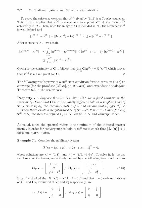
292 7. Nonlinear Systems and Numerical Optimization
To prove the existence we show that x(k) given by (7.17) is a Cauchy sequence.This in turn implies that x(k) is convergent to a point x()) / D0. Take x(0)
arbitrarily in D0. Then, since the image of G is included in D0, the sequence x(k)
is well defined and
&x(k+1) % x(k)& = &G(x(k))%G(x(k%1))& " $&x(k) % x(k%1)&.
After p steps, p ! 1, we obtain
&x(k+p) % x(k)& "p(
i=1
&x(k+i) % x(k+i%1)& "8$p%1 + . . . + 1
9&x(k+1) % x(k)&
" $k
1% $&x(1) % x(0)&.
Owing to the continuity of G it follows that limk$!
G(x(k)) = G(x())) which proves
that x()) is a fixed point for G. !
The following result provides a su"cient condition for the iteration (7.17) toconverge (for the proof see [OR70], pp. 299-301), and extends the analogousTheorem 6.3 in the scalar case.
Property 7.3 Suppose that G : D * Rn ( Rn has a fixed point x, in theinterior of D and that G is continuously di!erentiable in a neighborhood ofx,. Denote by JG the Jacobian matrix of G and assume that )(JG(x(,))) <1. Then there exists a neighborhood S of x, such that S * D and, for anyx(0) ! S, the iterates defined by (7.17) all lie in D and converge to x,.
As usual, since the spectral radius is the infimum of the induced matrixnorms, in order for convergence to hold it su"ces to check that +JG(x)+ < 1for some matrix norm.
Example 7.4 Consider the nonlinear system
F(x) =8x2
1 + x22 % 1, 2x1 + x2 % 1
9T = 0,
whose solutions are x)1 = (0, 1)T and x)
2 = (4/5,%3/5)T . To solve it, let us usetwo fixed-point schemes, respectively defined by the following iteration functions
G1(x) =
"
$1% x2
231% x2
1
%
' , G2(x) =
"
$1% x2
2%
31% x2
1
%
' . (7.18)
It can be checked that Gi(x)i ) = x)
i for i = 1, 2 and that the Jacobian matricesof G1 and G2, evaluated at x)
1 and x)2 respectively, are
JG1(x)1) =
"
$0 % 1
2
0 0
%
' , JG2(x)2) =
"
$0 % 1
2
43 0
%
' .

7.1 Solution of Systems of Nonlinear Equations 293
The spectral radii are %(JG1(x)1)) = 0 and %(JG2(x
)2)) =
32/3 0 0.817 < 1 so
that both methods are convergent in a suitable neighborhood of their respectivefixed points.
Running Program 59, with a tolerance of 10%10 on the maximum absolutedi"erence between two successive iterates, the first scheme converges to x)
1 in 9iterations, starting from x(0) = (%0.9, 0.9)T , while the second one converges tox)
2 in 115 iterations, starting from x(0) = (0.9, 0.9)T . The dramatic change inthe convergence behavior of the two methods can be explained in view of thedi"erence between the spectral radii of the corresponding iteration matrices. •
Remark 7.1 Newton’s method can be regarded as a fixed-point methodwith iteration function
GN (x) = x" J"1F (x)F(x). (7.19)
If we denote by r(k) = F(x(k)) the residual at step k, from (7.19) it turnsout that Newton’s method can be alternatively formulated as
KI" JGN (x(k))
LKx(k+1) " x(k)
L= "r(k).
This equation allows us to interpret Newton’s method as a preconditionedstationary Richardson method. This prompts introducing a parameter "k
in order to accelerate the convergence of the iterationKI" JGN (x(k))
LKx(k+1) " x(k)
L= ""kr(k).
The problem of how to select "k will be addressed in Section 7.2.6. !
An implementation of the fixed-point method (7.17) is provided in Pro-gram 59. We have denoted by dim the size of the nonlinear system andby Phi the variables containing the functional expressions of the iterationfunction G. In output, the vector alpha contains the approximation of thesought zero of F and the vector res contains the sequence of the maximumnorms of the residuals of F(x(k)).
Program 59 - fixposys : Fixed-point method for nonlinear systems
function [alpha, res, nit]=fixposys(dim, x0, nmax, toll, Phi, F)x = x0; alpha=[x’]; res = 0;for k=1:dim,
r=abs(eval(F(k,:))); if (r > res), res = r; endend;nit = 0; residual(1)=res;while ((nit <= nmax) & (res >= toll)),
nit = nit + 1;for k = 1:dim, xnew(k) = eval(Phi(k,:)); endx = xnew; res = 0; alpha=[alpha;x]; x=x’;for k = 1:dim,
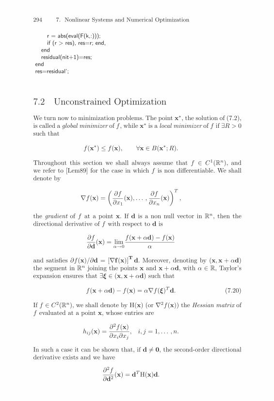
294 7. Nonlinear Systems and Numerical Optimization
r = abs(eval(F(k,:)));if (r > res), res=r; end,
endresidual(nit+1)=res;
endres=residual’;
7.2 Unconstrained Optimization
We turn now to minimization problems. The point x,, the solution of (7.2),is called a global minimizer of f , while x, is a local minimizer of f if -R > 0such that
f(x,) & f(x), #x ! B(x,;R).
Throughout this section we shall always assume that f ! C1(Rn), andwe refer to [Lem89] for the case in which f is non di!erentiable. We shalldenote by
5f(x) =4.f
.x1(x), . . . ,
.f
.xn(x)
5T
,
the gradient of f at a point x. If d is a non null vector in Rn, then thedirectional derivative of f with respect to d is
.f
.d(x) = lim
!&0
f(x + "d)" f(x)"
and satisfies .f(x)/.d = [5f(x)]T d. Moreover, denoting by (x,x + "d)the segment in Rn joining the points x and x + "d, with " ! R, Taylor’sexpansion ensures that -% ! (x,x + "d) such that
f(x + "d)" f(x) = "5f(%)Td. (7.20)
If f ! C2(Rn), we shall denote by H(x) (or 52f(x)) the Hessian matrix off evaluated at a point x, whose entries are
hij(x) =.2f(x).xi.xj
, i, j = 1, . . . , n.
In such a case it can be shown that, if d '= 0, the second-order directionalderivative exists and we have
.2f
.d2 (x) = dTH(x)d.

7.2 Unconstrained Optimization 295
For a suitable % ! (x,x + d) we also have
f(x + d)" f(x) = 5f(x)Td +12dTH(%)d.
Existence and uniqueness of solutions for (7.2) are not guaranteed in Rn.Nevertheless, the following optimality conditions can be proved.
Property 7.4 Let x, ! Rn be a local minimizer of f and assume thatf ! C1(B(x,;R)) for a suitable R > 0. Then 5f(x,) = 0. Moreover,if f ! C2(B(x,;R)) then H(x,) is positive semidefinite. Conversely, ifx, ! B(x,;R) and H(x,) is positive definite, then x, is a local minimizerof f in B(x,;R).
A point x, such that 5f(x,) = 0, is said to be a critical point for f . Thiscondition is necessary for optimality to hold. However, this condition alsobecomes su"cient if f is a convex function on Rn, i.e., such that #x,y ! Rn
and for any " ! [0, 1]
f ["x + (1" ")y] & "f(x) + (1" ")f(y). (7.21)
For further and more general existence results, see [Ber82].
7.2.1 Direct Search MethodsIn this section we deal with direct methods for solving problem (7.2), whichonly require f to be continuous. In later sections, we shall introduce theso-called descent methods, which also involve values of the derivatives of fand have, in general, better convergence properties.
Direct methods are employed when f is not di!erentiable or if the com-putation of its derivatives is a nontrivial task. They can also be used toprovide an approximate solution to employ as an initial guess for a descentmethod. For further details, we refer to [Wal75] and [Wol78].
The Hooke and Jeeves Method
Assume we are searching for the minimizer of f starting from a given initialpoint x(0) and requiring that the error on the residual is less than a certainfixed tolerance /. The Hooke and Jeeves method computes a new point x(1)
using the values of f at suitable points along the orthogonal coordinatedirections around x(0). The method consists of two steps: an explorationstep and an advancing step.
The exploration step starts by evaluating f(x(0) +h1e1), where e1 is thefirst vector of the canonical basis of Rn and h1 is a positive real number tobe suitably chosen.
If f(x(0) + h1e1) < f(x(0)), then a success is recorded and the startingpoint is moved in x(0) +h1e1, from which an analogous check is carried outat point x(0) + h1e1 + h2e2 with h2 ! R+.

296 7. Nonlinear Systems and Numerical Optimization
If, instead, f(x(0) + h1e1) ) f(x(0)), then a failure is recorded and asimilar check is performed at x(0) " h1e1. If a success is registered, themethod explores, as previously, the behavior of f in the direction e2 startingfrom this new point, while, in case of a failure, the method passes directlyto examining direction e2, keeping x(0) as starting point for the explorationstep.
To achieve a certain accuracy, the step lengths hi must be selected insuch a way that the quantities
|f(x(0) ± hjej)" f(x(0)|, j = 1, . . . , n (7.22)
have comparable sizes.The exploration step terminates as soon as all the n Cartesian directions
have been examined. Therefore, the method generates a new point, y(0),after at most 2n+1 functional evaluations. Only two possibilities may arise:
1. y(0) = x(0). In such a case, if maxi=1,... ,n
hi & / the method terminates
and yields the approximate solution x(0). Otherwise, the step lengthshi are halved and another exploration step is performed starting fromx(0);
2. y(0) '= x(0). If maxi=1,... ,n
|hi| < /, then the method terminates yielding
y(0) as an approximate solution, otherwise the advancing step starts.The advancing step consists of moving further from y(0) along thedirection y(0) " x(0) (which is the direction that recorded the maxi-mum decrease of f during the exploration step), rather then simplysetting y(0) as a new starting point x(1).
This new starting point is instead set equal to 2y(0)"x(0). From thispoint a new series of exploration moves is started. If this explorationleads to a point y(1) such that f(y(1)) < f(y(0) " x(0)), then a newstarting point for the next exploration step has been found, otherwisethe initial guess for further explorations is set equal to y(1) = y(0) "x(0).
The method is now ready to restart from the point x(1) just com-puted.
Program 60 provides an implementation of the Hooke and Jeeves method.The input parameters are the size n of the problem, the vector h of theinitial steps along the Cartesian directions, the variable f containing thefunctional expression of f in terms of the components x(1), . . . , x(n), theinitial point x0 and the stopping tolerance toll equal to /. In output, thecode returns the approximate minimizer of f , x, the value minf attained byf at x and the number of iterations needed to compute x up to the desiredaccuracy. The exploration step is performed by Program 61.
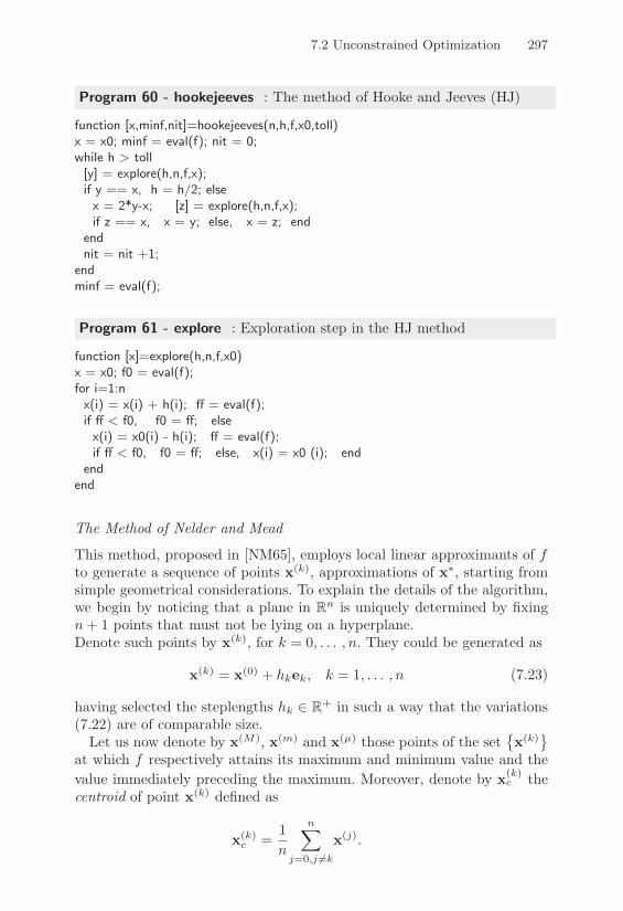
7.2 Unconstrained Optimization 297
Program 60 - hookejeeves : The method of Hooke and Jeeves (HJ)
function [x,minf,nit]=hookejeeves(n,h,f,x0,toll)x = x0; minf = eval(f); nit = 0;while h > toll[y] = explore(h,n,f,x);if y == x, h = h/2; elsex = 2*y-x; [z] = explore(h,n,f,x);if z == x, x = y; else, x = z; end
endnit = nit +1;
endminf = eval(f);
Program 61 - explore : Exploration step in the HJ method
function [x]=explore(h,n,f,x0)x = x0; f0 = eval(f);for i=1:nx(i) = x(i) + h(i); ! = eval(f);if ! < f0, f0 = !; elsex(i) = x0(i) - h(i); ! = eval(f);if ! < f0, f0 = !; else, x(i) = x0 (i); end
endend
The Method of Nelder and Mead
This method, proposed in [NM65], employs local linear approximants of fto generate a sequence of points x(k), approximations of x,, starting fromsimple geometrical considerations. To explain the details of the algorithm,we begin by noticing that a plane in Rn is uniquely determined by fixingn + 1 points that must not be lying on a hyperplane.Denote such points by x(k), for k = 0, . . . , n. They could be generated as
x(k) = x(0) + hkek, k = 1, . . . , n (7.23)
having selected the steplengths hk ! R+ in such a way that the variations(7.22) are of comparable size.
Let us now denote by x(M), x(m) and x(µ) those points of the set/x(k)0
at which f respectively attains its maximum and minimum value and thevalue immediately preceding the maximum. Moreover, denote by x(k)
c thecentroid of point x(k) defined as
x(k)c =
1n
n(
j=0,j '=k
x(j).
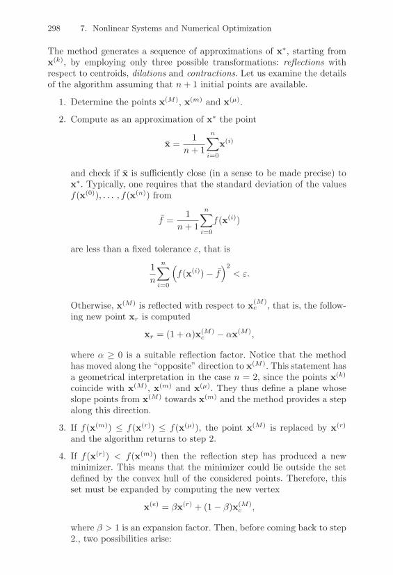
298 7. Nonlinear Systems and Numerical Optimization
The method generates a sequence of approximations of x,, starting fromx(k), by employing only three possible transformations: reflections withrespect to centroids, dilations and contractions. Let us examine the detailsof the algorithm assuming that n + 1 initial points are available.
1. Determine the points x(M), x(m) and x(µ).
2. Compute as an approximation of x, the point
x =1
n + 1
n(
i=0
x(i)
and check if x is su"ciently close (in a sense to be made precise) tox,. Typically, one requires that the standard deviation of the valuesf(x(0)), . . . , f(x(n)) from
f =1
n + 1
n(
i=0
f(x(i))
are less than a fixed tolerance +, that is
1n
n(
i=0
Kf(x(i))" f
L2< +.
Otherwise, x(M) is reflected with respect to x(M)c , that is, the follow-
ing new point xr is computed
xr = (1 + ")x(M)c " "x(M),
where " ) 0 is a suitable reflection factor. Notice that the methodhas moved along the “opposite” direction to x(M). This statement hasa geometrical interpretation in the case n = 2, since the points x(k)
coincide with x(M), x(m) and x(µ). They thus define a plane whoseslope points from x(M) towards x(m) and the method provides a stepalong this direction.
3. If f(x(m)) & f(x(r)) & f(x(µ)), the point x(M) is replaced by x(r)
and the algorithm returns to step 2.
4. If f(x(r)) < f(x(m)) then the reflection step has produced a newminimizer. This means that the minimizer could lie outside the setdefined by the convex hull of the considered points. Therefore, thisset must be expanded by computing the new vertex
x(e) = #x(r) + (1" #)x(M)c ,
where # > 1 is an expansion factor. Then, before coming back to step2., two possibilities arise:

7.2 Unconstrained Optimization 299
4a. if f(x(e)) < f(x(m)) then x(M) is replaced by x(e);4b. f(x(e)) ) f(x(m)) then x(M) is replaced by x(r) since f(x(r)) <
f(x(m)).
5. If f(x(r)) > f(x(µ)) then the minimizer probably lies within a subsetof the convex hull of points
/x(k)0 and, therefore, two di!erent ap-
proaches can be pursued to contract this set. If f(x(r)) < f(x(M)),the contraction generates a new point of the form
x(co) = 'x(r) + (1" ')x(M)c , ' ! (0, 1),
otherwise,
x(co) = 'x(M) + (1" ')x(M)c , ' ! (0, 1),
Finally, before returning to step 2., if f(x(co)) < f(x(M)) and f(x(co)) <f(x(r)), the point x(M) is replaced by x(co), while if f(x(co)) ) f(x(M))or if f(x(co)) > f(x(r)), then n new points x(k) are generated, withk = 1, . . . , n, by halving the distances between the original pointsand x(0).
As far as the choice of the parameters ", # and ' is concerned, the followingvalues are empirically suggested in [NM65]: " = 1, # = 2 and ' = 1/2. Theresulting scheme is known as the Simplex method (that must not be con-fused with a method sharing the same name used in linear programming),since the set of the points x(k), together with their convex combinations,form a simplex in Rn.
The convergence rate of the method is strongly a!ected by the orientationof the starting simplex. To address this concern, in absence of informationabout the behavior of f , the initial choice (7.23) turns out to be satisfactoryin most cases.
We finally mention that the Simplex method is the basic ingredient ofthe MATLAB function fmins for function minimization in n dimensions.
Example 7.5 Let us compare the performances of the Simplex method with theHooke and Jeeves method, in the minimization of the Rosembrock function
f(x) = 100(x2 % x21)
2 + (1% x1)2. (7.24)
This function has a minimizer at (1, 1)T and represents a severe benchmark fortesting numerical methods in minimization problems. The starting point for bothmethods is set equal to x(0) = (%1.2, 1)T , while the step sizes are taken equalto h1 = 0.6 and h2 = 0.5, in such a way that (7.23) is satisfied. The stoppingtolerance on the residual is set equal to 10%4. For the implementation of Simplexmethod, we have used the MATLAB function fmins.
Figure 7.2 shows the iterates computed by the Hooke and Jeeves method (ofwhich one in every ten iterates have been reported, for the sake of clarity) and by

300 7. Nonlinear Systems and Numerical Optimization
!1.5 !1 !0.5 0 0.5 1 1.50
0.2
0.4
0.6
0.8
1
1.2
1.4
1.6
1.8
2
FIGURE 7.2. Convergence histories of the Hooke and Jeeves method(crossed-line) and the Simplex method (circled-line). The level curves of the min-imized function (7.24) are reported in dashed line
the Simplex method, superposed to the level curves of the Rosembrock function.The graph demonstrates the di!culty of this benchmark: actually, the functionis like a curved, narrow valley, which attains its minimum along the parabola ofequation x2
1 % x2 = 0.The Simplex method converges in only 165 iterations, while 935 are needed for
the Hooke and Jeeves method to converge. The former scheme yields a solutionequal to (0.999987, 0.999978)T , while the latter gives the vector (0.9655, 0.9322)T .•
7.2.2 Descent MethodsIn this section we introduce iterative methods that are more sophisticatedthan those examined in Section 7.2.1. They can be formulated as follows:
given an initial vector x(0) ! Rn, compute for k ) 0 until convergence
x(k+1) = x(k) + "kd(k), (7.25)
where d(k) is a suitably chosen direction and "k is a positive parameter(called stepsize) that measures the step along the direction d(k). This di-rection d(k) is a descent direction if
d(k)T5f(x(k)) < 0 if 5f(x(k)) '= 0,
d(k) = 0 if 5f(x(k)) = 0.(7.26)
A descent method is a method like (7.25), in which the vectors d(k) aredescent directions.
Property (7.20) ensures that there exists "k > 0, su"ciently small, suchthat
f(x(k) + "kd(k)) < f(x(k)), (7.27)
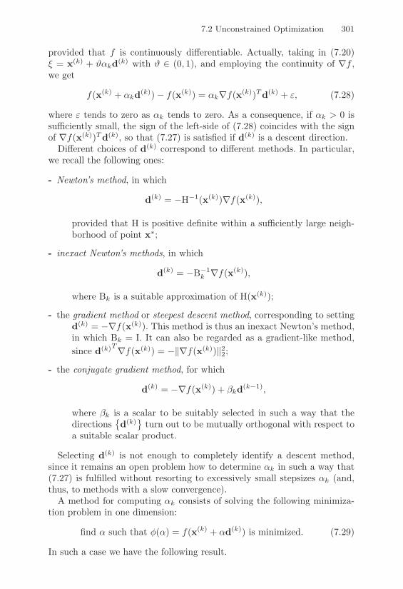
7.2 Unconstrained Optimization 301
provided that f is continuously di!erentiable. Actually, taking in (7.20)* = x(k) + ,"kd(k) with , ! (0, 1), and employing the continuity of 5f ,we get
f(x(k) + "kd(k))" f(x(k)) = "k5f(x(k))Td(k) + +, (7.28)
where + tends to zero as "k tends to zero. As a consequence, if "k > 0 issu"ciently small, the sign of the left-side of (7.28) coincides with the signof 5f(x(k))Td(k), so that (7.27) is satisfied if d(k) is a descent direction.
Di!erent choices of d(k) correspond to di!erent methods. In particular,we recall the following ones:
- Newton’s method, in which
d(k) = "H"1(x(k))5f(x(k)),
provided that H is positive definite within a su"ciently large neigh-borhood of point x,;
- inexact Newton’s methods, in which
d(k) = "B"1k 5f(x(k)),
where Bk is a suitable approximation of H(x(k));
- the gradient method or steepest descent method, corresponding to settingd(k) = "5f(x(k)). This method is thus an inexact Newton’s method,in which Bk = I. It can also be regarded as a gradient-like method,since d(k)T5f(x(k)) = "+5f(x(k))+22;
- the conjugate gradient method, for which
d(k) = "5f(x(k)) + #kd(k"1),
where #k is a scalar to be suitably selected in such a way that thedirections
/d(k)0 turn out to be mutually orthogonal with respect to
a suitable scalar product.
Selecting d(k) is not enough to completely identify a descent method,since it remains an open problem how to determine "k in such a way that(7.27) is fulfilled without resorting to excessively small stepsizes "k (and,thus, to methods with a slow convergence).
A method for computing "k consists of solving the following minimiza-tion problem in one dimension:
find " such that 4(") = f(x(k) + "d(k)) is minimized. (7.29)
In such a case we have the following result.

302 7. Nonlinear Systems and Numerical Optimization
Theorem 7.3 Consider the descent method (7.25). If at the generic stepk, the parameter "k is set equal to the exact solution of (7.29), then thefollowing orthogonality property holds
5f(x(k+1))Td(k) = 0.
Proof. Let $k be a solution to (7.29). Then, the first derivative of 3, given by
3(($) =n(
i=1
1f1xi
(x(k) + $kd(k))11$
(x(k)i + $d(k)
i ) = 8f(x(k) + $kd(k))Td(k),
vanishes at $ = $k. The thesis then follows, recalling the definition of x(k+1). !
Unfortunately, except for in special cases (which are nevetherless quiterelevant, see Section 7.2.4), providing an exact solution of (7.29) is not fea-sible, since this is a nonlinear problem. One possible strategy consists ofapproximating f along the straight line x(k) + "d(k) through an interpo-lating polynomial and then minimizing this polynomial (see the quadraticinterpolation Powell methods and cubic interpolation Davidon methods in[Wal75]).
Generally speaking, a process that leads to an approximate solution to(7.29) is said to be a line search technique and is addressed in the nextsection.
7.2.3 Line Search TechniquesThe methods that we are going to deal with in this section, are iterativetechniques that terminate as soon as some accuracy stopping criterion on"k is satisfied. We shall assume that (7.26) holds.
Practical experience reveals that it is not necessary to solve accuratelyfor (7.29) in order to devise e"cient methods, rather, it is crucial to enforcesome limitation on the step lengths (and, thus, on the admissible values for"k). Actually, without introducing any limitation, a reasonable request on"k would seem be that the new iterate x(k+1) satisfies the inequality
f(x(k+1)) < f(x(k)), (7.30)
where x(k) and d(k) have been fixed. For this purpose, the procedure basedon starting from a (su"ciently large) value of the step length "k and halvethis value until (7.30) is fulfilled, can yield completely wrong results (see,[DS83]).
More stringent criteria than (7.30) should be adopted in the choice ofpossible values for "k. To this end, we notice that two kinds of di"cultiesarise with the above examples: a slow descent rate of the sequence and theuse of small stepsizes.
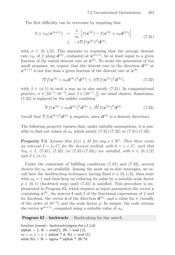
7.2 Unconstrained Optimization 303
The first di"culty can be overcome by requiring that
0 ) vM (x(k+1)) =1"k
Vf(x(k))" f(x(k) + "kd(k))
W
) "(5f(x(k))Td(k),(7.31)
with ( ! (0, 1/2). This amounts to requiring that the average descentrate vM of f along d(k), evaluated at x(k+1), be at least equal to a givenfraction of the initial descent rate at x(k). To avoid the generation of toosmall stepsizes, we require that the descent rate in the direction d(k) atx(k+1) is not less than a given fraction of the descent rate at x(k)
|5f(x(k) + "kd(k))Td(k)| & #|5f(x(k))Td(k)|, (7.32)
with # ! ((, 1) in such a way as to also satisfy (7.31). In computationalpractice, ( ! [10"5, 10"1] and # ! [10"1, 1
2 ] are usual choices. Sometimes,(7.32) is replaced by the milder condition
5f(x(k) + "kd(k))Td(k) ) #5f(x(k))Td(k) (7.33)
(recall that 5f(x(k))Td(k) is negative, since d(k) is a descent direction).
The following property ensures that, under suitable assumptions, it is pos-sible to find out values of "k which satisfy (7.31)-(7.32) or (7.31)-(7.33).
Property 7.5 Assume that f(x) ) M for any x ! Rn. Then there existsan interval I = [c, C] for the descent method, with 0 < c < C, such that#"k ! I, (7.31), (7.32) (or (7.31)-(7.33)) are satisfied, with ( ! (0, 1/2)and # ! ((, 1).
Under the constraint of fulfilling conditions (7.31) and (7.32), severalchoices for "k are available. Among the most up-to-date strategies, we re-call here the backtracking techniques: having fixed ( ! (0, 1/2), then startwith "k = 1 and then keep on reducing its value by a suitable scale factor) ! (0, 1) (backtrack step) until (7.31) is satisfied. This procedure is im-plemented in Program 62, which requires as input parameters the vector xcontaining x(k), the macros f and J of the functional expressions of f andits Jacobian, the vector d of the direction d(k), and a value for ( (usuallyof the order of 10"4) and the scale factor ). In output, the code returnsthe vector x(k+1), computed using a suitable value of "k.
Program 62 - backtrackr : Backtraking for line search
function [xnew]= backtrackr(sigma,rho,x,f,J,d)alphak = 1; fk = eval(f); Jfk = eval (J);xx = x; x = x + alphak * d; fk1 = eval (f);while fk1 > fk + sigma * alphak * Jfk’*d

304 7. Nonlinear Systems and Numerical Optimization
alphak = alphak*rho;x = xx + alphak*d;fk1 = eval(f);
end
Other commonly used strategies are those developed by Armijo and Gold-stein (see [Arm66], [GP67]). Both use ( ! (0, 1/2). In the Armijo formula,one takes "k = #mk ", where # ! (0, 1), " > 0 and mk is the first non-negative integer such that (7.31) is satisfied. In the Goldstein formula, theparameter "k is determined in such a way that
( & f(x(k) + "kd(k))" f(x(k))"k5f(x(k))Td(k) & 1" (. (7.34)
A procedure for computing "k that satisfies (7.34) is provided in [Ber82],Chapter 1. Of course, one can even choose "k = " for any k, which isclearly convenient when evaluating f is a costly task.
In any case, a good choice of the value " is mandatory. In this respect,one can proceed as follows. For a given value ", the second degree poly-nomial $2 along the direction d(k) is constructed, subject to the followinginterpolation constraints
$2(x(k)) = f(x(k)),
$2(x(k) + "d(k)) = f(x(k) + "d(k)),
$*2(x(k)) = 5f(x(k))Td(k).
Next, the value " is computed such that $2 is minimized, then, we let" = ".
7.2.4 Descent Methods for Quadratic FunctionsA case of remarkable interest, where the parameter "k can be exactly com-puted, is the problem of minimizing the quadratic function
f(x) =12xTAx" bTx, (7.35)
where A! Rn!n is a symmetric and positive definite matrix and b ! Rn.In such a case, as already seen in Section 4.3.3, a necessary condition forx, to be a minimizer for f is that x, is the solution of the linear system(3.2). Actually, it can be checked that if f is a quadratic function
5f(x) = Ax" b = "r, H(x) = A.
As a consequence, all gradient-like iterative methods developed in Section4.3.3 for linear systems, can be extended tout-court to solve minimizationproblems.

7.2 Unconstrained Optimization 305
In particular, having fixed a descent direction d(k), we can determinethe optimal value of the acceleration parameter "k that appears in (7.25),in such a way as to find the point where the function f , restricted to thedirection d(k), is minimized. Setting to zero the directional derivative, weget
dd"k
f(x(k) + "kd(k)) = "d(k)T r(k) + "kd(k)TAd(k) = 0
from which the following expression for "k is obtained
"k =d(k)T r(k)
d(k)TAd(k). (7.36)
The error introduced by the iterative process (7.25) at the k-th step is
+x(k+1) " x,+2A =8x(k+1) " x,9T A
8x(k+1) " x,9
= +x(k) " x,+2A + 2"kd(k)TA8x(k) " x,9 + "2
kd(k)TAd(k).
(7.37)
On the other hand +x(k) " x,+2A = r(k)TA"1r(k), so that from (7.37) itfollows that
+x(k+1) " x,+2A = )k+x(k) " x,+2A (7.38)
having denoted by )k = 1" (k, with
(k = (d(k)T r(k))2/4K
d(k)LT
Ad(k)Kr(k)
LTA"1r(k)
5.
Since A is symmetric and positive definite, (k is always positive. Moreover,it can be directly checked that )k is strictly less than 1, except when d(k)
is orthogonal to r(k), in which case )k = 1.The choice d(k) = r(k), which leads to the steepest descent method, pre-
vents this last circumstance from arising. In such a case, from (7.38) weget
+x(k+1) " x,+A &$max " $min
$max + $min+x(k) " x,+A (7.39)
having employed the following result.
Lemma 7.1 (Kantorovich inequality) Let A ! Rn!n be a symmetricpositive definite matrix whose eigenvalues with largest and smallest moduleare given by $max and $min, respectively. Then, #y ! Rn, y '= 0,
(yTy)2
(yTAy)(yTA"1y)) 4$max$min
($max + $min)2.
306 7. Nonlinear Systems and Numerical Optimization
It follows from (7.39) that, if A is ill-conditioned, the error reducing factorfor the steepest descent method is close to 1, yielding a slow convergence tothe minimizer x,. As done in Chapter 4, this drawback can be overcomeby introducing directions d(k) that are mutually A-conjugate, i.e.
d(k)TAd(m) = 0 if k '= m.
The corresponding methods enjoy the following finite termination property.
Property 7.6 A method for computing the minimizer x, of the quadraticfunction (7.35) which employs A-conjugate directions terminates after atmost n steps if the acceleration parameter "k is selected as in (7.36). More-over, for any k, x(k+1) is the minimizer of f over the subspace generatedby the vectors x(0),d(0), . . . ,d(k) and
r(k+1)Td(m) = 0 #m & k.
The A-conjugate directions can be determined by following the proce-dure described in Section 4.3.4. Letting d(0) = r(0), the conjugate gradientmethod for function minimization is
d(k+1) = r(k) + #kd(k),
#k = "r(k+1)TAd(k)
d(k)TAd(k)=
r(k+1)T r(k+1)
r(k)T r(k),
x(k+1) = x(k) + "kd(k).
It satisfies the following error estimate
+x(k) " x,+A & 2
63K2(A)" 1
3K2(A) + 1
7k
+x(0) " x,+A,
which can be improved by lowering the condition number of A, i.e., resort-ing to the preconditioning techniques that have been dealt with in Section4.3.2.
Remark 7.2 (The nonquadratic case) The conjugate gradient methodcan be extended to the case in which f is a non quadratic function. However,in such an event, the acceleration parameter "k cannot be exactly deter-mined a priori, but requires the solution of a local minimization problem.Moreover, the parameters #k can no longer be uniquely found. Among themost reliable formulae, we recall the one due to Fletcher-Reeves,
#1 = 0, #k =+5f(x(k))+22+5f(x(k"1))+22
, for k > 1

7.2 Unconstrained Optimization 307
and the one due to Polak-Ribiere
#1 = 0, #k =5f(x(k))T (5f(x(k))"5f(x(k"1)))
+5f(x(k"1))+22, for k > 1.
!
7.2.5 Newton-like Methods for Function MinimizationAn alternative is provided by Newton’s method, which di!ers from its ver-sion for nonlinear systems in that now it is no longer applied to f , but toits gradient.
Using the notation of Section 7.2.2, Newton’s method for function mini-mization amounts to computing, for k = 0, 1, . . . , until convergence
d(k) = "H"1k 5f(x(k)),
x(k+1) = x(k) + d(k),
(7.40)
where x(0) ! Rn is a given initial vector and having set Hk = H(x(k)). Themethod can be derived by truncating Taylor’s expansion of f(x(k)) at thesecond-order
f(x(k) + p) 1 f(x(k)) +5f(x(k))Tp +12pTHkp. (7.41)
Selecting p in (7.41) in such a way that the new vector x(k+1) = x(k) + psatisfies 5f(xk+1) = 0, we end up with method (7.40), which thus con-verges in one step if f is quadratic.
In the general case, a result analogous to Theorem 7.1 also holds for func-tion minimization. Method (7.40) is therefore locally quadratically conver-gent to the minimizer x,. However, it is not convenient to use Newton’smethod from the beginning of the computation, unless x(0) is su"cientlyclose to x,. Otherwise, indeed, Hk could not be invertible and the direc-tions d(k) could fail to be descent directions. Moreover, if Hk is not positivedefinite, nothing prevents the scheme (7.40) from converging to a saddlepoint or a maximizer, which are points where 5f is equal to zero. All thesedrawbacks, together with the high computational cost (recall that a linearsystem with matrix Hk must be solved at each iteration), prompt suit-ably modifying method (7.40), which leads to the so-called quasi-Newtonmethods.
A first modification, which applies to the case where Hk is not posi-tive definite, yields the so-called Newton’s method with shift. The idea isto prevent Newton’s method from converging to non-minimizers of f , byapplying the scheme to a new Hessian matrix Hk = Hk + µkIn, where, as

308 7. Nonlinear Systems and Numerical Optimization
usual, In denotes the identity matrix of order n and µk is selected in sucha way that Hk is positive definite. The problem is to determine the shiftµk with a reduced e!ort. This can be done, for instance, by applying theGershgorin theorem to the matrix Hk (see Section 5.1). For further detailson the subject, see [DS83] and [GMW81].
7.2.6 Quasi-Newton MethodsAt the generic k-th iteration, a quasi-Newton method for function mini-mization performs the following steps:
1. compute the Hessian matrix Hk, or a suitable approximation Bk;
2. find a descent direction d(k) (not necessarily coinciding with the di-rection provided by Newton’s method), using Hk or Bk;
3. compute the acceleration parameter "k;
4. update the solution, setting x(k+1) = x(k) + "kd(k), according to aglobal convergence criterion.
In the particular case where d(k) = "H"1k 5f(x(k)), the resulting scheme is
called the damped Newton’s method. To compute Hk or Bk, one can resortto either Newton’s method or secant-like methods, which will be consideredin Section 7.2.7.
The criteria for selecting the parameter "k, that have been discussed inSection 7.2.3, can now be usefully employed to devise globally convergentmethods. Property 7.5 ensures that there exist values of "k satisfying (7.31),(7.33) or (7.31), (7.32).
Let us then assume that a sequence of iterates x(k), generated by adescent method for a given x(0), converge to a vector x,. This vector willnot be, in general, a critical point for f . The following result gives someconditions on the directions d(k) which ensure that the limit x, of thesequence is also a critical point of f .
Property 7.7 (Convergence) Let f : Rn ( R be a continuously di!er-entiable function, and assume that there exists L > 0 such that
+5f(x)"5f(y)+2 & L+x" y+2.
Then, if/x(k)0 is a sequence generated by a gradient-like method which
fulfills (7.31) and (7.33), then, one (and only one) of the following eventscan occur:
1. 5f(x(k)) = 0 for some k;
2. limk&$
f(x(k)) = ",;

7.2 Unconstrained Optimization 309
3. limk&$
5f(x(k))Td(k)
+d(k)+2= 0.
Thus, unless the pathological cases where the directions d(k) become toolarge or too small with respect to 5f(x(k)) or, even, are orthogonal to5f(x(k)), any limit of the sequence
/x(k)0 is a critical point of f .
The convergence result for the sequence x(k) can also be extended to thesequence f(x(k)). Indeed, the following result holds.
Property 7.8 Let/x(k)0 be a convergent sequence generated by a gradient-
like method, i.e., such that any limit of the sequence is also a critical pointof f . If the sequence
/x(k)0 is bounded, then 5f(x(k)) tends to zero as
k (,.
For the proofs of the above results, see [Wol69] and [Wol71].
7.2.7 Secant-like methodsIn quasi-Newton methods the Hessian matrix H is replaced by a suitableapproximation. Precisely, the generic iterate is
x(k+1) = x(k) " B"1k 5f(x(k)) = x(k) + s(k).
Assume that f : Rn ( R is of class C2 on an open convex set D * Rn.In such a case, H is symmetric and, as a consequence, approximants Bk
of H ought to be symmetric. Moreover, if Bk were symmetric at a pointx(k), we would also like the next approximant Bk+1 to be symmetric atx(k+1) = x(k) + s(k).To generate Bk+1 starting from Bk, consider the Taylor expansion
5f(x(k)) = 5f(x(k+1)) + Bk+1(x(k) " x(k+1)),
from which we get
Bk+1s(k) = y(k), with y(k) = 5f(x(k+1))"5f(x(k)).
Using again a series expansion of B, we end up with the following first-orderapproximation of H
Bk+1 = Bk +(y(k) " Bks(k))cT
cT s(k) , (7.42)
where c ! Rn and having assumed that cT s(k) '= 0. We notice that takingc = s(k) yields Broyden’s method, already discussed in Section 7.1.4 in thecase of systems of nonlinear equations.
Since (7.42) does not guarantee that Bk+1 is symmetric, it must besuitably modified. A way for constructing a symmetric approximant Bk+1

310 7. Nonlinear Systems and Numerical Optimization
consists of choosing c = y(k) " Bks(k) in (7.42), assuming that (y(k) "Bks(k))T s(k) '= 0. By so doing, the following symmetric first-order approx-imation is obtained
Bk+1 = Bk +(y(k) " Bks(k))(y(k) " Bks(k))T
(y(k) " Bks(k))T s(k) . (7.43)
From a computational standpoint, disposing of an approximation for His not completely satisfactory, since the inverse of the approximation ofH appears in the iterative methods that we are dealing with. Using theSherman-Morrison formula (3.57), with Ck = B"1
k , yields the followingrecursive formula for the computation of the inverse
Ck+1 = Ck +(s(k) " Cky(k))(s(k) " Cky(k))T
(s(k) " Cky(k))Ty(k) , k = 0, 1, . . . (7.44)
having assumed that y(k) = Bs(k), where B is a symmetric nonsingularmatrix, and that (s(k) " Cky(k))Ty(k) '= 0.
An algorithm that employs the approximations (7.43) or (7.44), is po-tentially unstable when (s(k) " Cky(k))Ty(k) 1 0, due to rounding errors.For this reason, it is convenient to set up the previous scheme in a morestable form. To this end, instead of (7.42), we introduce the approximation
B(1)k+1 = Bk +
(y(k) " Bks(k))cT
cT s(k) ,
then, we define B(2)k+1 as being the symmetric part
B(2)k+1 =
B(1)k+1 + (B(1)
k+1)T
2.
The procedure can be iterated as follows
B(2j+1)k+1 = B(2j)
k+1 +(y(k) " B(2j)
k+1s(k))cT
cT s,
B(2j+2)k+1 =
B(2j+1)k+1 + (B(2j+1)
k+1 )T
2
(7.45)
with k = 0, 1, . . . and having set B(0)k+1 = Bk. It can be shown that the limit
as j tends to infinity of (7.45) is
limj&$
B(j) = Bk+1 = Bk +(y(k) " Bks(k))cT + c(y(k) " Bks(k))T
cT s(k)
" (y(k) " Bks(k))T s(k)
(cT s(k))2ccT ,
(7.46)

7.3 Constrained Optimization 311
having assumed that cT s(k) '= 0. If c = s(k), the method employing (7.46)is known as the symmetric Powell-Broyden method. Denoting by BSPB
the corresponding matrix Bk+1, it can be shown that BSPB is the uniquesolution to the problem:
find B such that +B" B+F is minimized,
where Bs(k) = y(k) and + · +F is the Frobenius norm.As for the error made approximating H(x(k+1)) with BSPB , it can be provedthat
+BSPB "H(x(k+1))+F & +Bk "H(x(k))+F + 3L+s(k)+,
where it is assumed that H is Lipschitz continuous, with Lipschitz constantL, and that the iterates x(k+1) and x(k) belong to D.
To deal with the particular case in which the Hessian matrix is not onlysymmetric but also positive definite, we refer to [DS83], Section 9.2.
7.3 Constrained Optimization
The simplest case of constrained optimization can be formulated as follows.Given f : Rn ( R,
minimize f(x), with x ! ( * Rn. (7.47)
More precisely, the point x, is said to be a global minimizer in ( if itsatisfies (7.47), while it is a local minimizer if -R > 0 such that
f(x,) & f(x), #x ! B(x,;R) * (.
Existence of solutions to problem (7.47) is, for instance, ensured by theWeierstrass theorem, in the case in which f is continuous and ( is a closedand bounded set. Under the assumption that ( is a convex set, the followingoptimality conditions hold.
Property 7.9 Let ( * Rn be a convex set, x, ! ( and f ! C1(B(x,;R)),for a suitable R > 0. Then:
1. if x, is a local minimizer of f then
5f(x,)T (x" x,) ) 0, #x ! (; (7.48)
2. moreover, if f is convex on ( (see (7.21)) and (7.48) is satisfied, thenx, is a global minimizer of f .
312 7. Nonlinear Systems and Numerical Optimization
We recall that f : ( ( R is a strongly convex function if -) > 0 suchthat
f ["x + (1" ")y] & "f(x) + (1" ")f(y)" "(1" "))+x" y+22, (7.49)
#x,y ! ( and #" ! [0, 1]. The following result holds.
Property 7.10 Let ( * Rn be a closed and convex set and f be a stronglyconvex function in (. Then there exists a unique local minimizer x, ! (.
Throughout this section, we refer to [Avr76], [Ber82], [CCP70], [Lue73] and[Man69], for the proofs of the quoted results and further details.
A remarkable instance of (7.47) is the following problem: given f : Rn ( R,
minimize f(x), under the constraint that h(x) = 0, (7.50)
where h : Rn ( Rm, with m & n, is a given function of componentsh1, . . . , hm. The analogues of critical points in problem (7.50) are calledthe regular points.
Definition 7.2 A point x, ! Rn, such that h(x,) = 0, is said to beregular if the column vectors of the Jacobian matrix Jh(x,) are linearlyindependent, having assumed that hi ! C1(B(x,;R)), for a suitable R > 0and i = 1, . . . ,m. !
Our aim now is to convert problem (7.50) into an unconstrained minimiza-tion problem of the form (7.2), to which the methods introduced in Section7.2 can be applied.
For this purpose, we introduce the Lagrangian function L : Rn+m ( R
L(x,&) = f(x) + &Th(x),
where the vector & is called the Lagrange multiplier. Moreover, let us de-note by JL the Jacobian matrix associated with L, but where the partialderivatives are only taken with respect to the variables x1, . . . , xn. The linkbetween (7.2) and (7.50) is then expressed by the following result.
Property 7.11 Let x, be a local minimizer for (7.50) and suppose that,for a suitable R > 0, f, hi ! C1(B(x,;R)), for i = 1, . . . ,m. Then thereexists a unique vector &, ! Rm such that JL(x,,&,) = 0.
Conversely, assume that x, ! Rn satisfies h(x,) = 0 and that, for asuitable R > 0 and i = 1, . . . ,m, f, hi ! C2(B(x,;R)). Let HL be thematrix of entries .2L/.xi.xj for i, j = 1, . . . , n. If there exists a vector&, ! Rm such that JL(x,,&,) = 0 and
zTHL(x,,&,)z > 0 #z '= 0, with 5h(x,)T z = 0,
then x, is a strict local minimizer of (7.50).

7.3 Constrained Optimization 313
The last class of problems that we are going to deal with includes the casewhere inequality constraints are also present, i.e.: given f : Rn ( R,
minimize f(x), under the constraint that h(x) = 0 and g(x) & 0,(7.51)
where h : Rn ( Rm, with m & n, and g : Rn ( Rr are two given functions.It is understood that g(x) & 0 means gi(x) & 0 for i = 1, . . . , r. Inequalityconstraints give rise to some extra formal complication with respect to thecase previously examined, but do not prevent converting the solution of(7.51) into the minimization of a suitable Lagrangian function.
In particular, Definition 7.2 becomes
Definition 7.3 Assume that hi, gj ! C1(B(x,;R)) for a suitable R >0 with i = 1, . . . ,m and j = 1, . . . , r, and denote by J (x,) the set ofindices j such that gj(x,) = 0. A point x, ! Rn such that h(x,) = 0 andg(x,) & 0 is said to be regular if the column vectors of the Jacobian matrixJh(x,) together with the vectors 5gj(x,), j ! J (x,) form a set of linearlyindependent vectors. !
Finally, an analogue of Property 7.11 holds, provided that the followingLagrangian function is used
M(x,&,µ) = f(x) + &Th(x) + µTg(x)
instead of L and that further assumptions on the constraints are made.For the sake of simplicity, we report in this case only the following nec-
essary condition for optimality of problem (7.51) to hold.
Property 7.12 Let x, be a regular local minimizer for (7.51) and supposethat, for a suitable R > 0, f, hi, gj ! C1(B(x,;R)) with i = 1, . . . ,m,j = 1, . . . , r. Then, there exist only two vectors &, ! Rm and µ, ! Rr,such that JM(x,,&,,µ,) = 0 with µ,
j ) 0 and µ,jgj(x,) = 0 #j = 1, . . . , r.
7.3.1 Kuhn-Tucker Necessary Conditions for NonlinearProgramming
In this section we recall some results, known as Kuhn-Tucker conditions[KT51], that ensure in general the existence of a local solution for the non-linear programming problem. Under suitable assumptions they also guar-antee the existence of a global solution. Throughout this section we supposethat a minimization problem can always be reformulated as a maximizationone.

314 7. Nonlinear Systems and Numerical Optimization
Let us consider the general nonlinear programming problem:
given f : Rn ( R,
maximize f(x), subject to
gi(x) & bi i = 1, . . . , l,
gi(x) ) bi i = l + 1, . . . , k,
gi(x) = bi i = k + 1, . . . ,m,
x ) 0.
(7.52)
A vector x that satisfies the constraints above is called a feasible solution of(7.52) and the set of the feasible solutions is called the feasible region. Weassume henceforth that f, gi ! C1(Rn), i = 1, . . . ,m, and define the setsI= = {i : gi(x,) = bi}, I '= = {i : gi(x,) '= bi}, J= = {i : x,
i = 0}, J> ={i : x,
i > 0}, having denoted by x, a local maximizer of f . We associatewith (7.52) the following Lagrangian
L(x,&) = f(x) +m(
i=1
$i [bi " gi(x)]"m+n(
i=m+1
$ixi"m.
The following result can be proved.
Property 7.13 (Kuhn-Tucker conditions I and II) If f has a con-strained local maximum at the point x = x,, it is necessary that a vector&, ! Rm+n exists such that (first Kuhn-Tucker condition)
5xL(x,,&,) & 0,
where strict equality holds for every component i ! J>. Moreover (secondKuhn-Tucker condition)
(5xL(x,,&,))T x, = 0.
The other two necessary Kuhn-Tucker conditions are as follows.
Property 7.14 Under the same hypothesis as in Property 7.13, the thirdKuhn-Tucker condition requires that:
5"L(x,,&,) ) 0 i = 1, . . . , l,
5"L(x,,&,) & 0 i = l + 1, . . . , k,
5"L(x,,&,) = 0 i = k + 1, . . . ,m.
Moreover (fourth Kuhn-Tucker condition)
(5"L(x,,&,))T x, = 0.

7.3 Constrained Optimization 315
It is worth noticing that the Kuhn-Tucker conditions hold provided thatthe vector &, exists. To ensure this, it is necessary to introduce a furthergeometric condition that is known as constraint qualification (see [Wal75],p. 48).
We conclude this section by the following fundamental theorem whichestablishes when the Kuhn-Tucker conditions become also su"cient for theexistence of a global maximizer for f .
Property 7.15 Assume that the function f in (7.52) is a concave func-tion (i.e., "f is convex) in the feasible region. Suppose also that the point(x,,&,) satisfies all the Kuhn-Tucker necessary conditions and that thefunctions gi for which $,i > 0 are convex while those for which $,i < 0 areconcave. Then f(x,) is the constrained global maximizer of f for problem(7.52).
7.3.2 The Penalty MethodThe basic idea of this method is to eliminate, partly or completely, theconstraints in order to transform the constrained problem into an uncon-strained one. This new problem is characterized by the presence of a pa-rameter that yields a measure of the accuracy at which the constraint isactually imposed.
Let us consider the constrained problem (7.50), assuming we are search-ing for the solution x, only in ( * Rn. Suppose that such a problem admitsat least one solution in ( and write it in the following penalized form
minimize L!(x) for x ! (, (7.53)
whereL!(x) = f(x) +
12"+h(x)+22.
The function L! : Rn ( R is called the penalized Lagrangian, and " iscalled the penalty parameter. It is clear that if the constraint was exactlysatisfied then minimizing f would be equivalent to minimizing L!.The penalty method is an iterative technique for solving (7.53).
For k = 0, 1, . . . , until convergence, one must solve the sequence of prob-lems
minimize L!k(x) with x ! (, (7.54)
where {"k} is an increasing monotonically sequence of positive penaltyparameters, such that "k (, as k (,. As a consequence, after choosing"k, at each step of the penalty process we have to solve a minimizationproblem with respect to the variable x, leading to a sequence of values x,
k,solutions to (7.54). By doing so, the objective function L!k(x) tends toinfinity, unless h(x) is equal to zero.

316 7. Nonlinear Systems and Numerical Optimization
The minimization problems can then be solved by one of the methodsintroduced in Section 7.2. The following property ensures the convergenceof the penalty method in the form (7.53).
Property 7.16 Assume that f : Rn ( R and h : Rn ( Rm, with m & n,are continuous functions on a closed set ( * Rn and suppose that thesequence of penalty parameters "k > 0 is monotonically divergent. Finally,let x,
k be the global minimizer of problem (7.54) at step k. Then, takingthe limit as k ( ,, the sequence x,
k converges to x,, which is a globalminimizer of f in ( and satisfies the constraint h(x,) = 0.
Regarding the selection of the parameters "k, it can be shown that largevalues of "k make the minimization problem in (7.54) ill-conditioned, thusmaking its solution quite prohibitive unless the initial guess is particularlyclose to x,. On the other hand, the sequence "k must not grow too slowly,since this would negatively a!ect the overall convergence of the method.
A choice that is commonly made in practice is to pick up a not too largevalue of "0 and then set "k = #"k"1 for k > 0, where # is an integernumber between 4 and 10 (see [Ber82]). Finally, the starting point for thenumerical method used to solve the minimization problem (7.54) can beset equal to the last computed iterate.
The penalty method is implemented in Program 63. This requires asinput parameters the functions f, h, an initial value alpha0 for the penaltyparameter and the number beta.
Program 63 - lagrpen : Penalty method
function [x,vinc,nit]=lagrpen(x0,alpha0,beta,f,h,toll)x = x0; [r,c]=size(h); vinc = 0;for i=1:r, vinc = max(vinc,eval(h(i,1:c))); endnorm2h=[’(’,h(1,1:c),’)ˆ2’];for i=2:r, norm2h=[norm2h,’+(’,h(i,1:c),’)ˆ2’]; endalpha = alpha0; options(1)=0; options(2)=toll*0.1; nit = 0;while vinc > tollg=[f,’+0.5*’,num2str(alpha,16),’*’,norm2h];[x]=fmins(g,x,options);vinc=0; nit = nit + 1;for i=1:r, vinc = max(vinc,eval(h(i,1:c))); endalpha=alpha*beta;
end
Example 7.6 Let us employ the penalty method to compute the minimizer off(x) = 100(x2 % x2
1)2 + (1 % x1)2 under the constraint h(x) = (x1 + 0.5)2 +(x2 + 0.5)2 % 0.25 = 0. The crosses in Figure 7.3 denote the sequence of iteratescomputed by Program 63 starting from x(0) = (1, 1)T and choosing $0 = 0.1, ) =6. The method converges in 12 iterations to the value x = (%0.2463,%0.0691)T ,satisfying the constraint up to a tolerance of 10%4. •

7.3 Constrained Optimization 317
!2 !1.5 !1 !0.5 0 0.5 1 1.5 2!2
!1.5
!1
!0.5
0
0.5
1
1.5
2
FIGURE 7.3. Convergence history of the penalty method in Example 7.6
7.3.3 The Method of Lagrange MultipliersA variant of the penalty method makes use of (instead of L!(x) in (7.53))the augmented Lagrangian function G! : Rm % Rn ( R given by
G!(x,&) = f(x) + &Th(x) +12"+h(x)+22, (7.55)
where & ! Rm is a Lagrange multiplier. Clearly, if x, is a solution to prob-lem (7.50), then it will also be a solution to (7.55), but with the advantage,with respect to (7.53), of disposing of the further degree of freedom &. Thepenalty method applied to (7.55) reads: for k = 0, 1, . . . , until convergence,solve the sequence of problems
minimize G!k(x,&k) for x ! (, (7.56)
where {&k} is a bounded sequence of unknown vectors in Rn, and theparameters "k are defined as above (notice that if &k were zero, then wewould recover method (7.54)).
Property 7.16 also holds for method (7.56), provided that the multipliersare assumed to be bounded. Notice that the existence of the minimizerof (7.56) is not guaranteed, even in the case where f has a unique globalminimizer (see Example 7.7). This circumstance can be overcome by addingfurther non quadratic terms to the augmented Lagrangian function (e.g.,of the form +h+p2, with p large).
318 7. Nonlinear Systems and Numerical Optimization
Example 7.7 Let us find the minimizer of f(x) = %x4 under the constraintx = 0. Such problem clearly admits the solution x) = 0. If, instead, one considersthe augmented Lagrangian function
L!k(x,#k) = %x4 + #kx +12$kx
2,
one finds that it no longer admits a minimum at x = 0, though vanishing there,for any $k di"erent from zero. •
As far as the choice of the multipliers is concerned, the sequence of vectors&k is typically assigned by the following formula
&k+1 = &k + "kh(x(k)),
where &0 is a given value while the sequence of "k can be set a priori ormodified during run-time.
As for the convergence properties of the method of Lagrange multipliers,the following local result holds.
Property 7.17 Assume that x, is a regular strict local minimizer of (7.50)and that:
1. f, hi ! C2(B(x,;R)) with i = 1, . . . ,m and for a suitable R > 0;
2. the pair (x,,&,) satisfies zTHG0(x,,&,)z > 0, #z '= 0 such thatJh(x,)T z = 0;
3. -" > 0 such that HG"(x,,&,) > 0.
Then, there exist three positive scalars %, ' and M such that, for any pair(&,") ! V =
/(&,") ! Rm+1 : +&" &,+2 < %", " ) "
0, the problem
minimize G!(x,&), with x ! B(x,; '),
admits a unique solution x(&,"), di!erentiable with respect to its argu-ments. Moreover, #(&,") ! V
+x(&,")" x,+2 &M+&" &,+2.
Under further assumptions (see [Ber82], Proposition 2.7), it can be provedthat the Lagrange multipliers method converges. Moreover, if "k (,, ask (,, then
limk&$
+&k+1 " &,+2+&k " &,+2
= 0.
and the convergence of the method is more than linear. In the case wherethe sequence "k has an upper bound, the method converges linearly.

7.4 Applications 319
Finally, we notice that, unlike the penalty method, it is no longer nec-essary that the sequence of "k tends to infinity. This, in turn, limits theill-conditioning of problem (7.56) as "k is growing. Another advantage con-cerns the convergence rate of the method, which turns out to be indepen-dent of the growth rate of the penalty parameter, in the case of the Lagrangemultipliers technique. This of course implies a considerable reduction of thecomputational cost.
The method of Lagrange multipliers is implemented in Program 64. Com-pared with Program 63, this further requires in input the initial valuelambda0 of the multiplier.
Program 64 - lagrmult : Method of Lagrange multipliers
function [x,vinc,nit]=lagrmult(x0,lambda0,alpha0,beta,f,h,toll)x = x0; [r,c]=size(h); vinc = 0; lambda = lambda0;for i=1:r, vinc = max(vinc,eval(h(i,1:c))); endnorm2h=[’(’,h(1,1:c),’)ˆ2’];for i=2:r, norm2h=[norm2h,’+(’,h(i,1:c),’)ˆ2’]; endalpha = alpha0; options(1)=0; options(2)=toll*0.1; nit = 0;while vinc > tolllh=[’(’,h(1,1:c),’)*’,num2str(lambda(1))];for i=2:r, lh=[lh,’+(’,h(i,1:c),’)*’,num2str(lambda(i))];endg=[f,’+0.5*’,num2str(alpha,16),’*’,norm2h,’+’,lh];[x]=fmins(g,x,options);vinc=0; nit = nit + 1;for i=1:r, vinc = max(vinc,eval(h(i,1:c))); endalpha=alpha*beta;for i=1:r, lambda(i)=lambda(i)+alpha*eval(h(i,1:c)); end
end
Example 7.8 We use the method of Lagrange multipliers to solve the prob-lem presented in Example 7.6. Set & = 10 and leave the remaining parametersunchanged. The method converges in 6 iterations and the crosses in Figure 7.4show the iterates computed by Program 64. The constraint is here satisfied upto machine precision. •
7.4 Applications
The two applications of this section are concerned with nonlinear systemsarising in the simulation of the electric potential in a semiconductor deviceand in the triangulation of a two-dimensional polygon.

320 7. Nonlinear Systems and Numerical Optimization
!1 !0.5 0 0.5 1
!1
!0.5
0
0.5
1
FIGURE 7.4. Convergence history for the method of Lagrange multipliers inExample 7.8
7.4.1 Solution of a Nonlinear System Arising fromSemiconductor Device Simulation
Let us consider the nonlinear system in the unknown u ! Rn
F(u) = Au + '(u)" b = 0, (7.57)
where A = ($/h)2tridiagn("1, 2"1), for h = 1/(n+1), 'i(u) = 2K sinh(ui)for i = 1, . . . , n, where $ and K are two positive constants and b ! Rn isa given vector. Problem (7.57) arises in the numerical simulation of semi-conductor devices in microelectronics, where u and b represent electricpotential and doping profile, respectively.
In Figure 7.5 (left) we show schematically the particular device consid-ered in the numerical example, a p " n junction diode of unit normalizedlength, subject to an external bias =V = Vb"Va, together with the dopingprofile of the device, normalized to 1 (right). Notice that bi = b(xi), fori = 1, . . . , n, where xi = ih. The mathematical model of the problem athand comprises a nonlinear Poisson equation for the electric potential andtwo continuity equations of advection-di!usion type, as those addressed inChapter 12, for the current densities. For the complete derivation of themodel and its analysis see, for instance, [Mar86] and [Jer96].Solving system (7.57) corresponds to finding the minimizer in Rn of thefunction f : Rn ( R defined as
f(u) =12uTAu + 2
n(
i=1
cosh(ui))" bTu. (7.58)
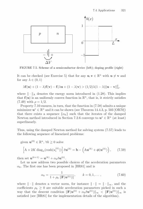
7.4 Applications 321
+
p n
!V
"
0 Lx
b(x)
"1
1
FIGURE 7.5. Scheme of a semiconductor device (left); doping profile (right)
It can be checked (see Exercise 5) that for any u,v ! Rn with u '= v andfor any $ ! (0, 1)
$f(u) + (1" $)f(v)" f($u + (1" $)v) > (1/2)$(1" $)+u" v+2A,
where + · +A denotes the energy norm introduced in (1.28). This impliesthat f(u) is an uniformly convex function in Rn, that is, it strictly satisfies(7.49) with ) = 1/2.
Property 7.10 ensures, in turn, that the function in (7.58) admits a uniqueminimizer u, ! Rn and it can be shown (see Theorem 14.4.3, p. 503 [OR70])that there exists a sequence {"k} such that the iterates of the dampedNewton method introduced in Section 7.2.6 converge to u, ! Rn (at least)superlinearly.
Thus, using the damped Newton method for solving system (7.57) leads tothe following sequence of linearized problems:
given u(0) ! Rn, #k ) 0 solveVA + 2K diagn(cosh(u(k)
i ))W%u(k) = b"
KAu(k) + '(u(k))
L, (7.59)
then set u(k+1) = u(k) + "k%u(k).Let us now address two possible choices of the acceleration parameters
"k. The first one has been proposed in [BR81] and is
"k =1
1 + )k +F(u(k))+, k = 0, 1, . . . , (7.60)
where + · + denotes a vector norm, for instance + · + = + · +$, and thecoe"cients )k ) 0 are suitable acceleration parameters picked in such away that the descent condition +F(u(k) + "k%u(k))+$ < +F(u(k))+$ issatisfied (see [BR81] for the implementation details of the algorithm).

322 7. Nonlinear Systems and Numerical Optimization
We notice that, as +F(u(k))+$ ( 0, (7.60) yields "k ( 1, thus recov-ering the full (quadratic) convergence of Newton’s method. Otherwise, astypically happens in the first iterations, +F(u(k))+$ 4 1 and "k is quiteclose to zero, with a strong reduction of the Newton variation (damping).As an alternative to (7.60), the sequence {"k} can be generated using thesimpler formula, suggested in [Sel84], Chapter 7
"k = 2"i(i"1)/2, k = 0, 1, . . . , (7.61)
where i is the first integer in the interval [1, Itmax] such that the descentcondition above is satisfied, Itmax being the maximum admissible numberof damping cycles for any Newton’s iteration (fixed equal to 10 in thenumerical experiments).As a comparison, both damped and standard Newton’s methods have beenimplemented, the former one with both choices (7.60) and (7.61) for thecoe"cients "k. In the case of Newton’s method, we have set in (7.59) "k = 1for any k ) 0.
The numerical examples have been performed with n = 49, bi = "1 fori & n/2 and the remaining values bi equal to 1. Moreover, we have taken$2 = 1.67 · 10"4, K = 6.77 · 10"6 and fixed the first n/2 components of theinitial vector u(0) equal to Va and the remaining ones equal to Vb, whereVa = 0 and Vb = 10.
The tolerance on the maximum change between two successive iterates,which monitors the convergence of damped Newton’s method (7.59), hasbeen set equal to 10"4.
100
101
102
10!6
10!4
10!2
100
102
104
(1)
(2)
(3)
0 2 4 6 8 100
0.1
0.2
0.3
0.4
0.5
0.6
0.7
0.8
0.9
1
FIGURE 7.6. Absolute error (left) and damping parameters $k (right). The errorcurve for standard Newton’s method is denoted by (1), while (2) and (3) refer todamped Newton’s method with the choices (7.61) and (7.60) for the coe!cients$k, respectively
Figure 7.6 (left) shows the log-scale absolute error for the three algorithmsas functions of the iteration number. Notice the rapid convergence of the

7.4 Applications 323
damped Newton’s method (8 and 10 iterations in the case of (7.60) and(7.61), respectively), compared with the extremely slow convergence of thestandard Newton’s method (192 iterations). Moreover, it is interesting toanalyze in Figure 7.6 (right) the plot of the sequences of parameters "k asfunctions of the iteration number.
The starred and the circled curves refer to the choices (7.60) and (7.61)for the coe"cients "k, respectively. As previously observed, the "k’s startfrom very small values, to converge quickly to 1 as the damped Newtonmethod (7.59) enters the attraction region of the minimizer x,.
7.4.2 Nonlinear Regularization of a Discretization GridIn this section we go back to the problem of regularizing a discretizationgrid that has been introduced in Section 3.14.2. There, we considered thetechnique of barycentric regularization, which leads to solving a linear sys-tem, typically of large size and featuring a sparse coe"cient matrix.
In this section we address two alternative techniques, denoted as reg-ularization by edges and by areas. The main di!erence with respect tothe method described in Section 3.14.2 lies in the fact that these new ap-proaches lead to systems of nonlinear equations.
Using the notation of Section 3.14.2, for each pair of nodes xj , xk ! Zi,denote by ljk the edge on the boundary .Pi of Pi which connects themand by xjk the midpoint of ljk, while for each triangle T ! Pi we denoteby xb,T the centroid of T . Moreover, let ni = dim(Zi) and denote for anygeometric entity (side or triangle) by | · | its measure in R1 or R2.
In the case of regularization by edges, we let
xi =
G
H(
ljk#)Pi
xjk|ljk|
I
J /|.Pi|, #xi ! Nh, (7.62)
while in the case of regularization by areas, we let
xi =
6(
T#Pi
xb,T |T |7
/|Pi|, #xi ! Nh. (7.63)
In both the regularization procedures we assume that xi = x()D)i if xi !
.D, that is, the nodes lying on the boundary of the domain D are fixed. Let-ting n = N"Nb be the number of internal nodes, relation (7.62) amounts tosolving the following two systems of nonlinear equations for the coordinates

324 7. Nonlinear Systems and Numerical Optimization
{xi} and {yi} of the internal nodes, with i = 1, . . . , n
xi "12
G
H(
ljk#)Pi
(xj + xk)|ljk|
I
J /(
ljk#)Pi
|ljk| = 0,
yi "12
G
H(
ljk#)Pi
(yj + yk)|ljk|
I
J /(
ljk#)Pi
|ljk| = 0.
(7.64)
Similarly, (7.63) leads to the following nonlinear systems, for i = 1, . . . , n
xi "13
6(
T#Pi
(x1,T + x2,T + x3,T )|T |7
/(
T#Pi
|T | = 0,
yi "13
6(
T#Pi
(y1,T + y2,T + y3,T )|T |7
/(
T#Pi
|T | = 0,(7.65)
where xs,T = (xs,T , ys,T ), for s = 1, 2, 3, are the coordinates of the verticesof each triangle T ! Pi. Notice that the nonlinearity of systems (7.64) and(7.65) is due to the presence of terms |ljk| and |T |.
Both systems (7.64) and (7.65) can be cast in the form (7.1), denoting,as usual, by fi the i-th nonlinear equation of the system, for i = 1, . . . , n.The complex functional dependence of fi on the unknowns makes it pro-hibitive to use Newton’s method (7.4), which would require the explicitcomputation of the Jacobian matrix JF.
A convenient alternative is provided by the nonlinear Gauss-Seidel method(see [OR70], Chapter 7), which generalizes the corresponding method pro-posed in Chapter 4 for linear systems and can be formulated as follows.
Denote by zi, for i = 1, . . . , n, either of the unknown xi or yi. Given theinitial vector z(0) = (z(0)
1 , . . . , z(0)n )T , for k = 0, 1, . . . until convergence,
solve
fi(z(k+1)1 , . . . , z(k+1)
i"1 , *, z(k)i+1, . . . , z
(k)n ) = 0, i = 1, . . . , n, (7.66)
then, set z(k+1)i = *. Thus, the nonlinear Gauss-Seidel method converts
problem (7.1) into the successive solution of n scalar nonlinear equations.In the case of system (7.64), each of these equations is linear in the unknownz(k+1)i (since * does not explicitly appear in the bracketed term at the right
side of (7.64)). This allows for its exact solution in one step.In the case of system (7.65), the equation (7.66) is genuinely nonlinear
with respect to *, and is solved taking one step of a fixed-point iteration.The nonlinear Gauss-Seidel (7.66) has been implemented in MATLAB
to solve systems (7.64) and (7.65) in the case of the initial triangulationshown in Figure 7.7 (left). Such a triangulation covers the external regionof a two dimensional wing section of type NACA 2316. The grid containsNT = 534 triangles and n = 198 internal nodes.
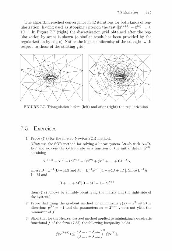
7.5 Exercises 325
The algorithm reached convergence in 42 iterations for both kinds of reg-ularization, having used as stopping criterion the test +z(k+1) " z(k)+$ &10"4. In Figure 7.7 (right) the discretization grid obtained after the reg-ularization by areas is shown (a similar result has been provided by theregularization by edges). Notice the higher uniformity of the triangles withrespect to those of the starting grid.
FIGURE 7.7. Triangulation before (left) and after (right) the regularization
7.5 Exercises1. Prove (7.8) for the m-step Newton-SOR method.
[Hint: use the SOR method for solving a linear system Ax=b with A=D-E-F and express the k-th iterate as a function of the initial datum x(0),obtaining
x(k+1) = x(0) + (Mk+1 % I)x(0) + (Mk + . . . + I)B%1b,
where B= -%1(D%-E) and M = B%1-%1 [(1% -)D + -F ]. Since B%1A =I%M and
(I + . . . + Mk)(I%M) = I%Mk+1
then (7.8) follows by suitably identifying the matrix and the right-side ofthe system.]
2. Prove that using the gradient method for minimizing f(x) = x2 with thedirections p(k) = %1 and the parameters $k = 2%k+1, does not yield theminimizer of f .
3. Show that for the steepest descent method applied to minimizing a quadraticfunctional f of the form (7.35) the following inequality holds
f(x(k+1)) "4#max % #min
#max + #min
52
f(x(k)),

326 7. Nonlinear Systems and Numerical Optimization
where #max,#min are the eigenvalues of maximum and minimum module,respectively, of the matrix A that appears in (7.35).[Hint: proceed as done for (7.38).]
4. Check that the parameters $k of Exercise 2 do not fulfill the conditions(7.31) and (7.32).
5. Consider the function f : Rn , R introduced in (7.58) and check that it isuniformly convex on Rn, that is
#f(u) + (1% #)f(v)% f(#u + (1% #)v) > (1/2)#(1% #)&u% v&2A
for any u, v / Rn with u $= v and 0 < # < 1.[Hint: notice that cosh(·) is a convex function.]
6. To solve the nonlinear system)***+
***,
% 181
cosx1 +19x2
2 +13
sinx3 = x1
13
sinx1 +13
cosx3 = x2
%19
cosx1 +13x2 +
16
sinx3 = x3,
use the fixed-point iteration x(n+1) = '(x(n)), where x = (x1, x2, x3)T and'(x) is the left-hand side of the system. Analyze the convergence of theiteration to compute the fixed point ( = (0, 1/3, 0)T .[Solution: the fixed-point method is convergent since &'(()&! = 1/2.]
7. Using Program 50 implementing Newton’s method, determine the globalmaximizer of the function
f(x) = e%x22 % 1
4cos(2x)
and analyze the performance of the method (input data: xv=1; toll=1e-6;nmax=500). Solve the same problem using the following fixed-point iteration
x(k+1) = g(xk) with g(x) = sin(2x)
"
$ ex22 (x sin(2x) + 2 cos(2x))% 22 (x sin(2x) + 2 cos(2x))
%
' .
Analyze the performance of this second scheme, both theoretically andexperimentally, and compare the results obtained using the two methods.[Solution: the function f has a global maximum at x = 0. This point isa double zero for f (. Thus, Newton’s method is only linearly convergent.Conversely, the proposed fixed-point method is third-order convergent.]

8Polynomial Interpolation
This chapter is addressed to the approximation of a function which is knownthrough its nodal values.
Precisely, given m+1 pairs (xi, yi), the problem consists of finding a func-tion ' = '(x) such that '(xi) = yi for i = 0, . . . ,m, yi being some givenvalues, and say that ' interpolates {yi} at the nodes {xi}. We speak aboutpolynomial interpolation if ' is an algebraic polynomial, trigonometric ap-proximation if ' is a trigonometric polynomial or piecewise polynomialinterpolation (or spline interpolation) if ' is only locally a polynomial.
The numbers yi may represent the values attained at the nodes xi by afunction f that is known in closed form, as well as experimental data. In theformer case, the approximation process aims at replacing f with a simplerfunction to deal with, in particular in view of its numerical integrationor derivation. In the latter case, the primary goal of approximation is toprovide a compact representation of the available data, whose number isoften quite large.
Polynomial interpolation is addressed in Sections 8.1 and 8.2, while piece-wise polynomial interpolation is introduced in Sections 8.3, 8.4 and 8.5. Fi-nally, univariate and parametric splines are addressed in Sections 8.6 and8.7. Interpolation processes based on trigonometric or algebraic orthogonalpolynomials will be considered in Chapter 10.

328 8. Polynomial Interpolation
8.1 Polynomial Interpolation
Let us consider n + 1 pairs (xi, yi). The problem is to find a polynomial$m ! Pm, called an interpolating polynomial, such that
$m(xi) = amxmi + . . . + a1xi + a0 = yi i = 0, . . . , n. (8.1)
The points xi are called interpolation nodes. If n '= m the problem is overor under-determined and will be addressed in Section 10.7.1. If n = m, thefollowing result holds.
Theorem 8.1 Given n+1 distinct points x0, . . . , xn and n+1 correspond-ing values y0, . . . , yn, there exists a unique polynomial $n ! Pn such that$n(xi) = yi for i = 0, . . . , n.
Proof. To prove existence, let us use a constructive approach, providing anexpression for (n. Denoting by {li}ni=0 a basis for Pn, then (n admits a repre-sentation on such a basis of the form (n(x) =
!ni=0 bili(x) with the property
that
(n(xi) =n(
j=0
bj lj(xi) = yi, i = 0, . . . , n. (8.2)
If we define
li / Pn : li(x) =n1
j=0j &=i
x% xj
xi % xji = 0, . . . , n, (8.3)
then li(xj) = !ij and we immediately get from (8.2) that bi = yi.The polynomials {li, i = 0, . . . , n} form a basis for Pn (see Exercise 1). As a con-sequence, the interpolating polynomial exists and has the following form (calledLagrange form)
(n(x) =n(
i=0
yili(x). (8.4)
To prove uniqueness, suppose that another interpolating polynomial 'm of de-gree m " n exists, such that 'm(xi) = yi for i = 0, ..., n. Then, the di"erencepolynomial (n%'m vanishes at n+1 distinct points xi and thus coincides withthe null polynomial. Therefore, 'm = (n.
An alternative approach to prove existence and uniqueness of (n is providedin Exercise 2. !
It can be checked that (see Exercise 3)
$n(x) =n(
i=0
0n+1(x)(x" xi)0*
n+1(xi)yi (8.5)

8.1 Polynomial Interpolation 329
where 0n+1 is the nodal polynomial of degree n + 1 defined as
0n+1(x) =n1
i=0
(x" xi). (8.6)
Formula (8.4) is called the Lagrange form of the interpolating polynomial,while the polynomials li(x) are the characteristic polynomials. In Figure8.1 we show the characteristic polynomials l2(x), l3(x) and l4(x), in thecase of degree n = 6, on the interval [-1,1] where equally spaced nodes aretaken, including the end points.
!1 !0.5 0 0.5 1!1.5
!1
!0.5
0
0.5
1
1.5
ll l2 3 4
FIGURE 8.1. Lagrange characteristic polynomials
Notice that |li(x)| can be greater than 1 within the interpolation interval.If yi = f(xi) for i = 0, . . . , n, f being a given function, the interpolating
polynomial $n(x) will be denoted by $nf(x).
8.1.1 The Interpolation ErrorIn this section we estimate the interpolation error that is made when re-placing a given function f with its interpolating polynomial $nf at thenodes x0, x1, . . . , xn (for further results, we refer the reader to [Wen66],[Dav63]).
Theorem 8.2 Let x0, x1, . . . , xn be n+1 distinct nodes and let x be a pointbelonging to the domain of a given function f . Assume that f ! Cn+1(Ix),where Ix is the smallest interval containing the nodes x0, x1, . . . , xn and x.Then the interpolation error at the point x is given by
En(x) = f(x)"$nf(x) =f (n+1)(*)(n + 1)!
0n+1(x), (8.7)
where * ! Ix and 0n+1 is the nodal polynomial of degree n + 1.

330 8. Polynomial Interpolation
Proof. The result is obviously true if x coincides with any of the interpola-tion nodes. Otherwise, define, for any t / Ix, the function G(t) = En(t) %-n+1(t)En(x)/-n+1(x). Since f / C(n+1)(Ix) and -n+1 is a polynomial, thenG / C(n+1)(Ix) and it has n + 2 distinct zeros in Ix, since
G(xi) = En(xi)% -n+1(xi)En(x)/-n+1(x) = 0, i = 0, . . . , n
G(x) = En(x)% -n+1(x)En(x)/-n+1(x) = 0.
Then, thanks to the mean value theorem, G( has n + 1 distinct zeros and, byrecursion, G(j) admits n + 2 % j distinct zeros. As a consequence, G(n+1) has aunique zero, which we denote by /. On the other hand, since E(n+1)
n (t) = f (n+1)(t)and -(n+1)
n+1 (x) = (n + 1)! we get
G(n+1)(t) = f (n+1)(t)% (n + 1)!-n+1(x)
En(x),
which, evaluated at t = /, gives the desired expression for En(x). !
8.1.2 Drawbacks of Polynomial Interpolation on EquallySpaced Nodes and Runge’s Counterexample
In this section we analyze the behavior of the interpolation error (8.7) asn tends to infinity. For this purpose, for any function f ! C0([a, b]), defineits maximum norm
+f+$ = maxx#[a,b]
|f(x)|. (8.8)
Then, let us introduce a lower triangular matrix X of infinite size, called theinterpolation matrix on [a, b], whose entries xij , for i, j = 0, 1, . . . , representpoints of [a, b], with the assumption that on each row the entries are alldistinct.
Thus, for any n ) 0, the n + 1-th row of X contains n + 1 distinctvalues that we can identify as nodes, so that, for a given function f , wecan uniquely define an interpolating polynomial $nf of degree n at thosenodes (any polynomial $nf depends on X, as well as on f).
Having fixed f and an interpolation matrix X, let us define the interpo-lation error
En,$(X) = +f "$nf+$, n = 0, 1, . . . (8.9)
Next, denote by p,n ! Pn the best approximation polynomial, for which
E,n = +f " p,n+$ & +f " qn+$ #qn ! Pn.
The following comparison result holds (for the proof, see [Riv74]).

8.1 Polynomial Interpolation 331
Property 8.1 Let f ! C0([a, b]) and X be an interpolation matrix on [a, b].Then
En,$(X) & E,n (1 + %n(X)) , n = 0, 1, . . . (8.10)
where %n(X) denotes the Lebesgue constant of X, defined as
%n(X) =
AAAAAA
n(
j=0
|l(n)j |
AAAAAA$
, (8.11)
and where l(n)j ! Pn is the j-th characteristic polynomial associated with
the n + 1-th row of X, that is, satisfying l(n)j (xnk) = %jk, j, k = 0, 1, . . .
Since E,n does not depend on X, all the information concerning the e!ects
of X on En,$(X) must be looked for in %n(X). Although there exists aninterpolation matrix X, such that %n(X) is minimized, it is not in general asimple task to determine its entries explicitly. We shall see in Section 10.3,that the zeros of the Chebyshev polynomials provide on the interval ["1, 1]an interpolation matrix with a very small value of the Lebesgue constant.
On the other hand, for any possible choice of X, there exists a constantC > 0 such that (see [Erd61])
%n(X) >2&
log(n + 1)" C, n = 0, 1, . . .
This property shows that %n(X) (, as n(,. This fact has importantconsequences: in particular, it can be proved (see [Fab14]) that, given aninterpolation matrix X on an interval [a, b], there always exists a continuousfunction f in [a, b], such that $nf does not converge uniformly (that is, inthe maximum norm) to f . Thus, polynomial interpolation does not allow forapproximating any continuous function, as demonstrated by the followingexample.
Example 8.1 (Runge’s counterexample) Suppose we approximate the fol-lowing function
f(x) =1
1 + x2 , %5 " x " 5 (8.12)
using Lagrange interpolation on equally spaced nodes. It can be checked thatsome points x exist within the interpolation interval such that
limn$!
|f(x)%(nf(x)| $= 0.
In particular, Lagrange interpolation diverges for |x| > 3.63 . . . . This phenomenonis particularly evident in the neighborhood of the end points of the interpolationinterval, as shown in Figure 8.2, and is due to the choice of equally spaced nodes.We shall see in Chapter 10 that resorting to suitably chosen nodes will allow foruniform convergence of the interpolating polynomial to the function f to hold. •

332 8. Polynomial Interpolation
!5 !4 !3 !2 !1 0 1 2 3 4 5!0.5
0
0.5
1
1.5
2
FIGURE 8.2. Lagrange interpolation on equally spaced nodes for the functionf(x) = 1/(1 + x2): the interpolating polynomials (5f and (10f are shown indotted and dashed line, respectively
8.1.3 Stability of Polynomial Interpolation
Let us consider a set of function valuesR
Df(xi)S
which is a perturbationof the data f(xi) relative to the nodes xi, with i = 0, . . . , n, in an interval[a, b]. The perturbation may be due, for instance, to the e!ect of roundingerrors, or may be caused by an error in the experimental measure of thedata.
Denoting by $nDf the interpolating polynomial on the set of values Df(xi),
we have
+$nf "$nDf+$ = max
a%x%b
>>>>>>
n(
j=0
(f(xj)" Df(xj))lj(x)
>>>>>>& %n(X) max
i=0,...,n|f(xi)" Df(xi)|.
As a consequence, small changes on the data give rise to small changeson the interpolating polynomial only if the Lebesgue constant is small.This constant plays the role of the condition number for the interpolationproblem.
As previously noticed, %n grows as n(, and in particular, in the caseof Lagrange interpolation on equally spaced nodes, it can be proved that(see [Nat65])
%n(X) 1 2n+1
en log n
where e 1 2.7183 is the naeperian number. This shows that, for n large,this form of interpolation can become unstable. Notice also that so far wehave completely neglected the errors generated by the interpolation processin constructing $nf . However, it can be shown that the e!ect of such errorsis generally negligible (see [Atk89]).
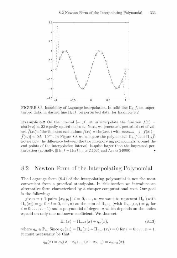
8.2 Newton Form of the Interpolating Polynomial 333
!1 !0.5 0 0.5 1!1.5
!1
!0.5
0
0.5
1
1.5
2
2.5
FIGURE 8.3. Instability of Lagrange interpolation. In solid line (21f , on unper-turbed data, in dashed line (21 Df , on perturbed data, for Example 8.2
Example 8.2 On the interval [%1, 1] let us interpolate the function f(x) =sin(2+x) at 22 equally spaced nodes xi. Next, we generate a perturbed set of val-ues Df(xi) of the function evaluations f(xi) = sin(2+xi) with maxi=0,...,21 |f(xi)%Df(xi)| 0 9.5 · 10%4. In Figure 8.3 we compare the polynomials (21f and (21 Df :notice how the di"erence between the two interpolating polynomials, around theend points of the interpolation interval, is quite larger than the impressed per-turbation (actually, &(21f %(21 Df&! 0 2.1635 and &21 0 24000). •
8.2 Newton Form of the Interpolating Polynomial
The Lagrange form (8.4) of the interpolating polynomial is not the mostconvenient from a practical standpoint. In this section we introduce analternative form characterized by a cheaper computational cost. Our goalis the following:
given n + 1 pairs {xi, yi}, i = 0, . . . , n, we want to represent $n (with$n(xi) = yi for i = 0, . . . , n) as the sum of $n"1 (with $n"1(xi) = yi fori = 0, . . . , n"1) and a polynomial of degree n which depends on the nodesxi and on only one unknown coe"cient. We thus set
$n(x) = $n"1(x) + qn(x), (8.13)
where qn ! Pn. Since qn(xi) = $n(xi)"$n"1(xi) = 0 for i = 0, . . . , n" 1,it must necessarily be that
qn(x) = an(x" x0) . . . (x" xn"1) = an0n(x).
334 8. Polynomial Interpolation
To determine the unknown coe"cient an, suppose that yi = f(xi), i =0, . . . , n, where f is a suitable function, not necessarily known in explicitform. Since $nf(xn) = f(xn), from (8.13) it follows that
an =f(xn)"$n"1f(xn)
0n(xn). (8.14)
The coe"cient an is called n-th the Newton divided di!erence and is gen-erally denoted by
an = f [x0, x1, . . . , xn] (8.15)
for n ) 1. As a consequence, (8.13) becomes
$nf(x) = $n"1f(x) + 0n(x)f [x0, x1, . . . , xn]. (8.16)
If we let y0 = f(x0) = f [x0] and 00 = 1, by recursion on n we can obtainfrom (8.16) the following formula
$nf(x) =n(
k=0
0k(x)f [x0, . . . , xk]. (8.17)
Uniqueness of the interpolating polynomial ensures that the above expres-sion yields the same interpolating polynomial generated by the Lagrangeform. Form (8.17) is commonly known as the Newton divided di!erenceformula for the interpolating polynomial.
Program 65 provides an implementation of Newton’s formula. The inputvectors x and y contain the interpolation nodes and the corresponding func-tional evaluations of f , respectively, while vector z contains the abscissaewhere the polynomial $nf is to be evaluated. This polynomial is stored inthe output vector f.
Program 65 - interpol : Lagrange polynomial using Newton’s formula
function [f] = interpol (x,y,z)[m n] = size(y);for j = 1:ma (:,1) = y (j,:)’;for i = 2:na (i:n,i) = ( a(i:n,i-1)-a(i-1,i-1) )./(x(i:n)-x(i-1))’;
endf(j,:) = a(n,n).*(z-x(n-1)) + a(n-1,n-1);for i = 2:n-1f(j,:) = f(j,:).*(z-x(n-i))+a(n-i,n-i);
endend
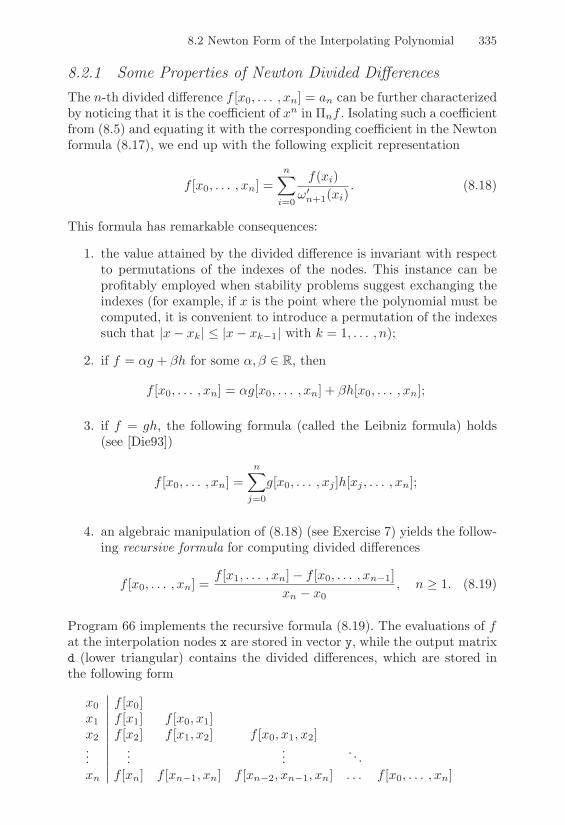
8.2 Newton Form of the Interpolating Polynomial 335
8.2.1 Some Properties of Newton Divided Di!erencesThe n-th divided di!erence f [x0, . . . , xn] = an can be further characterizedby noticing that it is the coe"cient of xn in $nf . Isolating such a coe"cientfrom (8.5) and equating it with the corresponding coe"cient in the Newtonformula (8.17), we end up with the following explicit representation
f [x0, . . . , xn] =n(
i=0
f(xi)0*n+1(xi)
. (8.18)
This formula has remarkable consequences:
1. the value attained by the divided di!erence is invariant with respectto permutations of the indexes of the nodes. This instance can beprofitably employed when stability problems suggest exchanging theindexes (for example, if x is the point where the polynomial must becomputed, it is convenient to introduce a permutation of the indexessuch that |x" xk| & |x" xk"1| with k = 1, . . . , n);
2. if f = "g + #h for some ",# ! R, then
f [x0, . . . , xn] = "g[x0, . . . , xn] + #h[x0, . . . , xn];
3. if f = gh, the following formula (called the Leibniz formula) holds(see [Die93])
f [x0, . . . , xn] =n(
j=0
g[x0, . . . , xj ]h[xj , . . . , xn];
4. an algebraic manipulation of (8.18) (see Exercise 7) yields the follow-ing recursive formula for computing divided di!erences
f [x0, . . . , xn] =f [x1, . . . , xn]" f [x0, . . . , xn"1]
xn " x0, n ) 1. (8.19)
Program 66 implements the recursive formula (8.19). The evaluations of fat the interpolation nodes x are stored in vector y, while the output matrixd (lower triangular) contains the divided di!erences, which are stored inthe following form
x0 f [x0]x1 f [x1] f [x0, x1]x2 f [x2] f [x1, x2] f [x0, x1, x2]...
......
. . .xn f [xn] f [xn"1, xn] f [xn"2, xn"1, xn] . . . f [x0, . . . , xn]
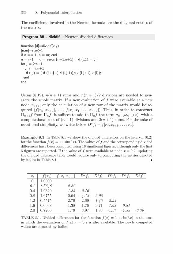
336 8. Polynomial Interpolation
The coe"cients involved in the Newton formula are the diagonal entries ofthe matrix.
Program 66 - dividif : Newton divided di!erences
function [d]=dividif(x,y)[n,m]=size(y);if n == 1, n = m; endn = n-1; d = zeros (n+1,n+1); d (:,1) = y’;for j = 2:n+1for i = j:n+1d (i,j) = ( d (i-1,j-1)-d (i,j-1))/(x (i-j+1)-x (i));
endend
Using (8.19), n(n + 1) sums and n(n + 1)/2 divisions are needed to gen-erate the whole matrix. If a new evaluation of f were available at a newnode xn+1, only the calculation of a new row of the matrix would be re-quired (f [xn, xn+1], . . . , f [x0, x1, . . . , xn+1]). Thus, in order to construct$n+1f from $nf , it su"ces to add to $nf the term an+10n+1(x), with acomputational cost of (n + 1) divisions and 2(n + 1) sums. For the sake ofnotational simplicity, we write below Drfi = f [xi, xi+1, . . . , xr].
Example 8.3 In Table 8.1 we show the divided di"erences on the interval (0,2)for the function f(x) = 1+sin(3x). The values of f and the corresponding divideddi"erences have been computed using 16 significant figures, although only the first5 figures are reported. If the value of f were available at node x = 0.2, updatingthe divided di"erence table would require only to computing the entries denotedby italics in Table 8.1. •
xi f(xi) f [xi, xi"1] D2fi D3fi D4fi D5fi D6fi0 1.0000
0.2 1.5646 2.820.4 1.9320 1.83 -2.460.8 1.6755 -0.64 -4.13 -2.081.2 0.5575 -2.79 -2.69 1.43 2.931.6 0.0038 -1.38 1.76 3.71 1.62 -0.812.0 0.7206 1.79 3.97 1.83 -1.17 -1.55 -0.36
TABLE 8.1. Divided di"erences for the function f(x) = 1 + sin(3x) in the casein which the evaluation of f at x = 0.2 is also available. The newly computedvalues are denoted by italics

8.2 Newton Form of the Interpolating Polynomial 337
Notice that f [x0, . . . , xn] = 0 for any f ! Pn"1. This property, how-ever, is not always verified numerically, since the computation of divideddi!erences might be highly a!ected by rounding errors.
Example 8.4 Consider again the divided di"erences for the function f(x) =1 + sin(3x) on the interval (0, 0.0002). The function behaves like 1 + 3x in asu!ciently small neighbourhood of 0, so that we expect to find smaller numbers asthe order of divided di"erences increases. However, the results obtained runningProgram 66, and shown in Table 8.2 in exponential notation up to the first 4significant figures (although 16 digits have been employed in the calculations),exhibit a substantially di"erent pattern. The small rounding errors introduced inthe computation of divided di"erences of low order have dramatically propagatedon the higher order divided di"erences. •
xi f(xi) f [xi, xi%1] D2fi D3fi D4fi D5fi0 1.0000
4.0e-5 1.0001 3.0008.0e-5 1.0002 3.000 -5.39e-41.2e-4 1.0004 3.000 -1.08e-3 -4.501.6e-4 1.0005 3.000 -1.62e-3 -4.49 1.80e+12.0e-4 1.0006 3.000 -2.15e-3 -4.49 -7.23 %1.2e + 5
TABLE 8.2. Divided di"erences for the function f(x) = 1+sin(3x) on the interval(0,0.0002). Notice the completely wrong value in the last column (it should beapproximately equal to 0), due to the propagation of rounding errors throughoutthe algorithm
8.2.2 The Interpolation Error Using Divided Di!erencesConsider the nodes x0, . . . , xn and let $nf be the interpolating polynomialof f on such nodes. Now let x be a node distinct from the previous ones;letting xn+1 = x, we denote by $n+1f the interpolating polynomial of fat the nodes xk, k = 0, . . . , n + 1. Using the Newton divided di!erencesformula, we get
$n+1f(t) = $nf(t) + (t" x0) . . . (t" xn)f [x0, . . . , xn, t].
Since $n+1f(x) = f(x), we obtain the following formula for the interpola-tion error at t = x
En(x) = f(x)"$nf(x) = $n+1f(x)"$nf(x)
= (x" x0) . . . (x" xn)f [x0, . . . , xn, x]
= 0n+1(x)f [x0, . . . , xn, x].
(8.20)

338 8. Polynomial Interpolation
Assuming f ! C(n+1)(Ix) and comparing (8.20) with (8.7), yields
f [x0, . . . , xn, x] =f (n+1)(*)(n + 1)!
(8.21)
for a suitable * ! Ix. Since (8.21) resembles the remainder of the Tay-lor series expansion of f , the Newton formula (8.17) for the interpolatingpolynomial is often regarded as being a truncated expansion around x0provided that |xn " x0| is not too big.
8.3 Piecewise Lagrange Interpolation
In Section 8.1.1 we have outlined the fact that, for equally spaced inter-polating nodes, uniform convergence of $nf to f is not guaranteed asn(,. On the other hand, using equally spaced nodes is clearly computa-tionally convenient and, moreover, Lagrange interpolation of low degree issu"ciently accurate, provided su"ciently small interpolation intervals areconsidered.
Therefore, it is natural to introduce a partition Th of [a, b] into K subin-tervals Ij = [xj , xj+1] of length hj , with h = max0%j%K"1 hj , such that[a, b] = 2K"1
j=0 Ij and then to employ Lagrange interpolation on each Ij
using n + 1 equally spaced nodesRx(i)j , 0 & i & n
Swith a small n.
For k ) 1, we introduce on Th the piecewise polynomial space
Xkh =
/v ! C0([a, b]) : v|Ij ! Pk(Ij)#Ij ! Th
0(8.22)
which is the space of the continuous functions over [a, b] whose restric-tions on each Ij are polynomials of degree & k. Then, for any continuousfunction f in [a, b], the piecewise interpolation polynomial $k
hf coincideson each Ij with the interpolating polynomial of f|Ij at the n + 1 nodesRx(i)j , 0 & i & n
S. As a consequence, if f ! Ck+1([a, b]), using (8.7) within
each interval we obtain the following error estimate
+f "$khf+$ & Chk+1 +f (k+1)+$. (8.23)
Note that a small interpolation error can be obtained even for low k pro-vided that h is su"ciently “small”.
Example 8.5 Let us go back to the function of Runge’s counterexample. Now,piecewise polynomials of degree k = 1 and k = 2 are employed. We check ex-perimentally for the behavior of the error as h decreases. In Table 8.3 we showthe absolute errors measured in the maximum norm over the interval [%5, 5] andthe corresponding estimates of the convergence order p with respect to h. Exceptwhen using an excessively small number of subintervals, the results confirm thetheoretical estimate (8.23), that is p = k + 1. •

8.3 Piecewise Lagrange Interpolation 339
h +f "$h1+$ p +f "$h
2+$ p5 0.4153 0.08352.5 0.1787 1.216 0.0971 -0.2171.25 0.0631 1.501 0.0477 1.0240.625 0.0535 0.237 0.0082 2.5370.3125 0.0206 1.374 0.0010 3.0380.15625 0.0058 1.819 1.3828e-04 2.8560.078125 0.0015 1.954 1.7715e-05 2.964
TABLE 8.3. Interpolation error for Lagrange piecewise interpolation of degreek = 1 and k = 2, in the case of Runge’s function (8.12); p denotes the trend ofthe exponent of h. Notice that, as h, 0, p, k + 1, as predicted by (8.23)
Besides estimate (8.23), convergence results in integral norms exist (see[QV94], [EEHJ96]). For this purpose, we introduce the following space
L2(a, b) =
)+
,f : (a, b) ( R,
b^
a
|f(x)|2dx < +,
_`
a , (8.24)
with
+f+L2(a,b) =
G
Hb^
a
|f(x)|2dx
I
J
1/2
. (8.25)
Formula (8.25) defines a norm for L2(a, b). (We recall that norms and semi-norms of functions can be defined in a manner similar to what was done inDefinition 1.17 in the case of vectors). We warn the reader that the integralof the function |f |2 in (8.24) has to be intended in the Lebesgue sense (see,e.g., [Rud83]). In particular, f needs not be continuous everywhere.
Theorem 8.3 Let 0 & m & k + 1, with k ) 1 and assume that f (m) !L2(a, b) for 0 & m & k + 1; then there exists a positive constant C, inde-pendent of h, such that
+(f "$khf)(m)+L2(a,b) & Chk+1"m+f (k+1)+L2(a,b). (8.26)
In particular, for k = 1, and m = 0 or m = 1, we obtain
+f "$1hf+L2(a,b) & C1h2+f **+L2(a,b),
+(f "$1hf)*+L2(a,b) & C2h+f **+L2(a,b),
(8.27)
for two suitable positive constants C1 and C2.
Proof. We only prove (8.27) and refer to [QV94], Chapter 3 for the proof of(8.26) in the general case.

340 8. Polynomial Interpolation
Define e = f % (1hf . Since e(xj) = 0 for all j = 0, . . . ,K, Rolle’s theorem
infers the existence of /j / (xj , xj+1), for j = 0, . . . ,K % 1 such that e((/j) = 0.Since (1
hf is a linear function on each Ij , for x / Ij we obtain
e((x) =^ x
(j
e(((s)ds =^ x
(j
f (((s)ds,
whence
|e((x)| "^ xj+1
xj
|f (((s)|ds, for x / [xj , xj+1]. (8.28)
We recall the Cauchy-Schwarz inequality>>>>
^ "
!
u(x)v(x)dx>>>> "
4^ "
!
u2(x)dx51/2 4^ "
!
v2(x)dx51/2
(8.29)
which holds if u, v / L2($,)). If we apply this inequality to (8.28) we obtain
|e((x)| "
G
\H
xj+1^
xj
12dx
I
]J
1/2 G
\H
xj+1^
xj
|f (((s)|2ds
I
]J
1/2
" h1/2
G
\H
xj+1^
xj
|f (((s)|2ds
I
]J
1/2
.
(8.30)
To find a bound for |e(x)|, we notice that
e(x) =^ x
xj
e((s)ds,
so that, applying (8.30), we get
|e(x)| "^ xj+1
xj
|e((s)|ds " h3/2
6^ xj+1
xj
|f (((s)|2ds71/2
. (8.31)
Thenxj+1^
xj
|e((x)|2dx " h2
xj+1^
xj
|f (((s)|2ds and
xj+1^
xj
|e(x)|2dx " h4
xj+1^
xj
|f (((s)|2ds,
from which, summing over the index j from 0 to K % 1 and taking the squareroot of both sides, we obtain
4^ b
a
|e((x)|2dx51/2
" h
4^ b
a
|f (((x)|2dx51/2
,
and 4^ b
a
|e(x)|2dx51/2
" h24^ b
a
|f (((x)|2dx51/2
,
which is the desired estimate (8.27), with C1 = C2 = 1. !

8.4 Hermite-Birko" Interpolation 341
8.4 Hermite-Birko" Interpolation
Lagrange polynomial interpolation can be generalized to the case in whichalso the values of the derivatives of a function f are available at some (orall) of the nodes xi.
Let us then suppose that (xi, f (k)(xi)) are given data, with i = 0, . . . , n,k = 0, . . . ,mi and mi ! N. Letting N =
!ni=0(mi + 1), it can be proved
(see [Dav63]) that, if the nodes {xi} are distinct, there exists a uniquepolynomial HN"1 ! PN"1, called the Hermite interpolation polynomial,such that
H(k)N"1(xi) = y(k)
i , i = 0, . . . , n k = 0, . . . ,mi,
of the form
HN"1(x) =n(
i=0
mi(
k=0
y(k)i Lik(x) (8.32)
where y(k)i = f (k)(xi), i = 0, . . . , n, k = 0, . . . ,mi.
The functions Lik ! PN"1 are called the Hermite characteristic polynomialsand are defined through the relations
dp
dxp(Lik)(xj) =
B1 if i = j and k = p,
0 otherwise.
Defining the polynomials
lij(x) =(x" xi)j
j!
n1
k=0k &=i
4x" xk
xi " xk
5mk+1
, i = 0, . . . , n, j = 0, . . . ,mi,
and letting Limi(x) = limi(x) for i = 0, . . . , n, we have the following recur-sive formula for the polynomials Lij
Lij(x) = lij(x)"mi(
k=j+1
l(k)ij (xi)Lik(x) j = mi " 1,mi " 2, . . . , 0.
As for the interpolation error, the following estimate holds
f(x)"HN"1(x) =f (N)(*)
N !(N (x) #x ! R
where * ! I(x;x0, . . . , xn) and (N is the polynomial of degree N definedby
(N (x) = (x" x0)m0+1(x" x1)m1+1 . . . (x" xn)mn+1. (8.33)
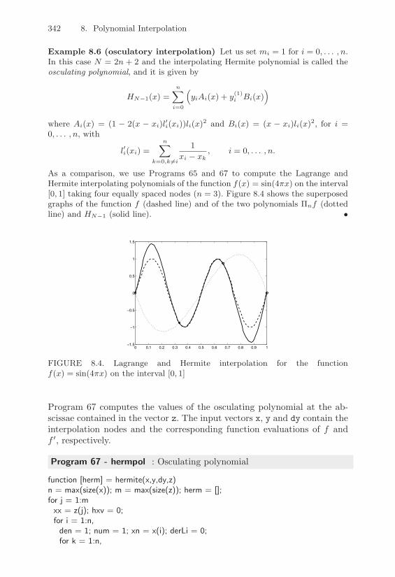
342 8. Polynomial Interpolation
Example 8.6 (osculatory interpolation) Let us set mi = 1 for i = 0, . . . , n.In this case N = 2n + 2 and the interpolating Hermite polynomial is called theosculating polynomial, and it is given by
HN%1(x) =n(
i=0
KyiAi(x) + y(1)
i Bi(x)L
where Ai(x) = (1 % 2(x % xi)l(i(xi))li(x)2 and Bi(x) = (x % xi)li(x)2, for i =0, . . . , n, with
l(i(xi) =n(
k=0,k #=i
1xi % xk
, i = 0, . . . , n.
As a comparison, we use Programs 65 and 67 to compute the Lagrange andHermite interpolating polynomials of the function f(x) = sin(4+x) on the interval[0, 1] taking four equally spaced nodes (n = 3). Figure 8.4 shows the superposedgraphs of the function f (dashed line) and of the two polynomials (nf (dottedline) and HN%1 (solid line). •
0 0.1 0.2 0.3 0.4 0.5 0.6 0.7 0.8 0.9 1!1.5
!1
!0.5
0
0.5
1
1.5
FIGURE 8.4. Lagrange and Hermite interpolation for the functionf(x) = sin(4+x) on the interval [0, 1]
Program 67 computes the values of the osculating polynomial at the ab-scissae contained in the vector z. The input vectors x, y and dy contain theinterpolation nodes and the corresponding function evaluations of f andf *, respectively.
Program 67 - hermpol : Osculating polynomial
function [herm] = hermite(x,y,dy,z)n = max(size(x)); m = max(size(z)); herm = [];for j = 1:mxx = z(j); hxv = 0;for i = 1:n,den = 1; num = 1; xn = x(i); derLi = 0;for k = 1:n,

8.5 Extension to the Two-Dimensional Case 343
if k ˜= i, num = num*(xx-x(k)); arg = xn-x(k);den = den*arg; derLi = derLi+1/arg;
endendLix2 = (num/den)ˆ2; p = (1-2*(xx-xn)*derLi)*Lix2;q = (xx-xn)*Lix2; hxv = hxv+(y(i)*p+dy(i)*q);endherm = [herm, hxv];
end
8.5 Extension to the Two-Dimensional Case
In this section we briefly address the extension of the previous concepts tothe two-dimensional case, referring to [SL89], [CHQZ88], [QV94] for moredetails. We denote by ( a bounded domain in R2 and by x = (x, y) thecoordinate vector of a point in (.
8.5.1 Polynomial InterpolationA particularly simple situation occurs when ( = [a, b] % [c, d], i.e., theinterpolation domain ( is the tensor product of two intervals. In such acase, introducing the nodes a = x0 < x1 < . . . < xn = b and c = y0 <y1 < . . . < ym = d, the interpolating polynomial $n,mf can be written as$n,mf(x, y) =
!ni=0
!mj=0 "ij li(x)lj(y), where li ! Pn, i = 0, . . . , n, and
lj ! Pm, j = 0, . . . ,m, are the characteristic one-dimensional Lagrangepolynomials with respect to the x and y variables respectively, and where"ij = f(xi, yj).
The drawbacks of one-dimensional Lagrange interpolation are inheritedby the two-dimensional case, as confirmed by the example in Figure 8.5.
Remark 8.1 (The general case) If ( is not a rectangular domain or ifthe interpolation nodes are not uniformly distributed over a Cartesian grid,the interpolation problem is di"cult to solve, and, generally speaking, it ispreferable to resort to a least-squares solution (see Section 10.7). We alsopoint out that in d dimensions (with d ) 2) the problem of finding aninterpolating polynomial of degree n with respect to each space variable onn + 1 distinct nodes might be ill-posed.
Consider, for example, a polynomial of degree 1 with respect to x and yof the form p(x, y) = a3xy+a2x+a1y+a0 to interpolate a function f at thenodes ("1, 0), (0,"1), (1, 0) and (0, 1). Although the nodes are distinct, theproblem (which is nonlinear) does not in general admit a unique solution;actually, imposing the interpolation constraints, we end up with a systemthat is satisfied by any value of the coe"cient a3. !

344 8. Polynomial Interpolation
!5
0
5
!5
0
5!0.1
0
0.1
0.2
0.3
0.4
0.5
!5
0
5
!5
0
5!2
0
2
4
6
8
FIGURE 8.5. Runge’s counterexample extended to the two-dimensional case:interpolating polynomial on a 61 6 nodes grid (left) and on a 111 11 nodes grid(right). Notice the change in the vertical scale between the two plots
8.5.2 Piecewise Polynomial InterpolationIn the multidimensional case, the higher flexibility of piecewise interpola-tion allows for easy handling of domains of complex shape. Let us supposethat ( is a polygon in R2. Then, ( can be partitioned into K nonover-lapping triangles (or elements) T , which define the so called triangulationof the domain which will be denoted by Th. Clearly, ( =
MT#Th
T . Suppose
that the maximum length of the edges of the triangles is less than a positivenumber h. As shown in Figure 8.6 (left), not any arbitrary triangulation isallowed. Precisely, the admissible ones are those for which any pair of nondisjoint triangles may have a vertex or an edge in common.
T
T2
1
2
TT
21
T1T2
T1 T
1
0 1
FT
:T:x
:y y
x
aT1 T
aT3
aT2
FIGURE 8.6. The left side picture shows admissible (above) and non admissible(below) triangulations while the right side picture shows the a!ne map from thereference triangle T to the generic element T / Th
Any element T ! Th, of area equal to |T |, is the image through the a"nemap x = FT (x) = BT x + bT of the reference triangle :T , of vertices (0,0),
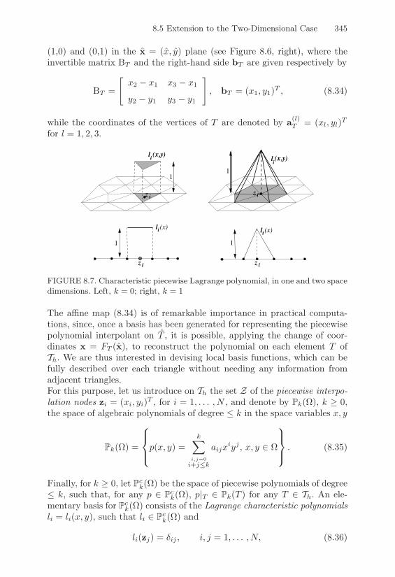
8.5 Extension to the Two-Dimensional Case 345
(1,0) and (0,1) in the x = (x, y) plane (see Figure 8.6, right), where theinvertible matrix BT and the right-hand side bT are given respectively by
BT =
Nx2 " x1 x3 " x1
y2 " y1 y3 " y1
O
, bT = (x1, y1)T , (8.34)
while the coordinates of the vertices of T are denoted by a(l)T = (xl, yl)T
for l = 1, 2, 3.
(x)
l (x,y)i
iz
z
1
i
li
1
z
iz
i
1
li(x,y)
1
li (x)
FIGURE 8.7. Characteristic piecewise Lagrange polynomial, in one and two spacedimensions. Left, k = 0; right, k = 1
The a"ne map (8.34) is of remarkable importance in practical computa-tions, since, once a basis has been generated for representing the piecewisepolynomial interpolant on T , it is possible, applying the change of coor-dinates x = FT (x), to reconstruct the polynomial on each element T ofTh. We are thus interested in devising local basis functions, which can befully described over each triangle without needing any information fromadjacent triangles.For this purpose, let us introduce on Th the set Z of the piecewise interpo-lation nodes zi = (xi, yi)T , for i = 1, . . . , N , and denote by Pk((), k ) 0,the space of algebraic polynomials of degree & k in the space variables x, y
Pk(() =
)*+
*,p(x, y) =
k(
i,j=0i+j%k
aijxiyj , x, y ! (
_*
*a. (8.35)
Finally, for k ) 0, let Pck(() be the space of piecewise polynomials of degree
& k, such that, for any p ! Pck((), p|T ! Pk(T ) for any T ! Th. An ele-
mentary basis for Pck(() consists of the Lagrange characteristic polynomials
li = li(x, y), such that li ! Pck(() and
li(zj) = %ij , i, j = 1, . . . , N, (8.36)
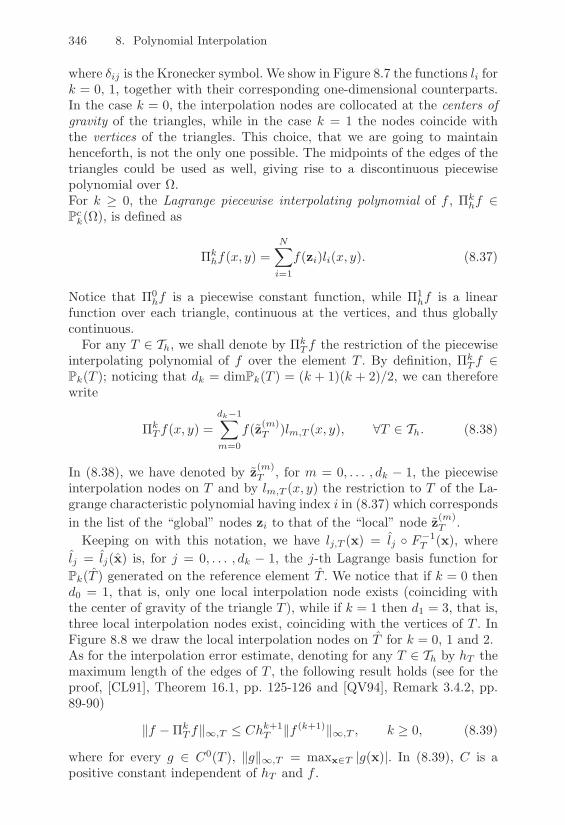
346 8. Polynomial Interpolation
where %ij is the Kronecker symbol. We show in Figure 8.7 the functions li fork = 0, 1, together with their corresponding one-dimensional counterparts.In the case k = 0, the interpolation nodes are collocated at the centers ofgravity of the triangles, while in the case k = 1 the nodes coincide withthe vertices of the triangles. This choice, that we are going to maintainhenceforth, is not the only one possible. The midpoints of the edges of thetriangles could be used as well, giving rise to a discontinuous piecewisepolynomial over (.For k ) 0, the Lagrange piecewise interpolating polynomial of f , $k
hf !Pck((), is defined as
$khf(x, y) =
N(
i=1
f(zi)li(x, y). (8.37)
Notice that $0hf is a piecewise constant function, while $1
hf is a linearfunction over each triangle, continuous at the vertices, and thus globallycontinuous.
For any T ! Th, we shall denote by $kT f the restriction of the piecewise
interpolating polynomial of f over the element T . By definition, $kT f !
Pk(T ); noticing that dk = dimPk(T ) = (k + 1)(k + 2)/2, we can thereforewrite
$kT f(x, y) =
dk"1(
m=0
f(z(m)T )lm,T (x, y), #T ! Th. (8.38)
In (8.38), we have denoted by z(m)T , for m = 0, . . . , dk " 1, the piecewise
interpolation nodes on T and by lm,T (x, y) the restriction to T of the La-grange characteristic polynomial having index i in (8.37) which correspondsin the list of the “global” nodes zi to that of the “local” node z(m)
T .Keeping on with this notation, we have lj,T (x) = lj 3 F"1
T (x), wherelj = lj(x) is, for j = 0, . . . , dk " 1, the j-th Lagrange basis function forPk(T ) generated on the reference element T . We notice that if k = 0 thend0 = 1, that is, only one local interpolation node exists (coinciding withthe center of gravity of the triangle T ), while if k = 1 then d1 = 3, that is,three local interpolation nodes exist, coinciding with the vertices of T . InFigure 8.8 we draw the local interpolation nodes on T for k = 0, 1 and 2.As for the interpolation error estimate, denoting for any T ! Th by hT themaximum length of the edges of T , the following result holds (see for theproof, [CL91], Theorem 16.1, pp. 125-126 and [QV94], Remark 3.4.2, pp.89-90)
+f "$kT f+$,T & Chk+1
T +f (k+1)+$,T , k ) 0, (8.39)
where for every g ! C0(T ), +g+$,T = maxx#T |g(x)|. In (8.39), C is apositive constant independent of hT and f .

8.5 Extension to the Two-Dimensional Case 347
FIGURE 8.8. Local interpolation nodes on T ; left, k = 0, center k = 1, right,k = 2
Let us assume that the triangulation Th is regular, i.e., there exists apositive constant ( such that
maxT#Th
hT
)T& (,
where #T ! Th, )T is the diameter of the inscribed circle to T , Then, itis possible to derive from (8.39) the following interpolation error estimateover the whole domain (
+f "$khf+$," & Chk+1+f (k+1)+$,", k ) 0, #f ! Ck+1(().
(8.40)
The theory of piecewise interpolation is a basic tool of the finite elementmethod, a computational technique that is widely used in the numericalapproximation of partial di!erential equations (see Chapter 12 for the one-dimensional case and [QV94] for a complete presentation of the method).
Example 8.7 We compare the convergence of the piecewise polynomial interpo-lation of degree 0, 1 and 2, on the function f(x, y) = e%(x2+y2) on ) = (%1, 1)2.We show in Table 8.4 the error Ek = &f %(k
hf&!,!, for k = 0, 1, 2, and the orderof convergence pk as a function of the mesh size h = 2/N for N = 2, . . . , 32.Clearly, linear convergence is observed for interpolation of degree 0 while theorder of convergence is quadratic with respect to h for interpolation of degree 1and cubic for interpolation of degree 2. •
h E0 p0 E1 p1 E2 p21 0.4384 0.2387 0.01612 0.2931 0.5809 0.1037 1.2028 1.6678 · 10"3 3.263914 0.1579 0.8924 0.0298 1.7990 2.8151 · 10"4 2.566718 0.0795 0.9900 0.0077 1.9524 3.5165 · 10"5 3.001116 0.0399 0.9946 0.0019 2.0189 4.555 · 10"6 2.9486
TABLE 8.4. Convergence rates and orders for piecewise interpolations of degree0, 1 and 2
348 8. Polynomial Interpolation
8.6 Approximation by Splines
In this section we address the matter of approximating a given function us-ing splines, which allow for a piecewise interpolation with a global smooth-ness.
Definition 8.1 Let x0, . . . , xn, be n + 1 distinct nodes of [a, b], with a =x0 < x1 < . . . < xn = b. The function sk(x) on the interval [a,b] is a splineof degree k relative to the nodes xj if
sk|[xj ,xj+1] ! Pk, j = 0, 1, . . . , n" 1 (8.41)
sk ! Ck"1[a, b]. (8.42)
!
Denoting by Sk the space of splines sk on [a, b] relative to n + 1 distinctnodes, then dimSk = n+k. Obviously, any polynomial of degree k on [a, b]is a spline; however, in the practice a spline is represented by a di!erentpolynomial on each subinterval and for this reason there could be a discon-tinuity in its k-th derivative at the internal nodes x1, . . . , xn"1. The nodesfor which this actually happens are called active nodes.
It is simple to check that conditions (8.41) and (8.42) do not su"ce tocharacterize a spline of degree k. Indeed, the restriction sk,j = sk|[xj ,xj+1]can be represented as
sk,j(x) =k(
i=0
sij(x" xj)i, if x ! [xj , xj+1] (8.43)
so that (k + 1)n coe"cients sij must be determined. On the other hand,from (8.42) it follows that
s(m)k,j"1(xj) = s(m)
k,j (xj), j = 1, . . . , n" 1, m = 0, ..., k " 1
which amounts to setting k(n " 1) conditions. As a consequence, the re-maining degrees of freedom are (k + 1)n" k(n" 1) = k + n.Even if the spline were interpolatory, that is, such that sk(xj) = fj forj = 0, . . . , n, where f0, . . . , fn are given values, there would still be k " 1unsaturated degrees of freedom. For this reason further constraints areusually imposed, which lead to:
1. periodic splines, if
s(m)k (a) = s(m)
k (b), m = 0, 1, . . . , k " 1; (8.44)

8.6 Approximation by Splines 349
2. natural splines, if for k = 2l " 1, with l ) 2
s(l+j)k (a) = s(l+j)
k (b) = 0, j = 0, 1, . . . , l " 2. (8.45)
From (8.43) it turns out that a spline can be conveniently represented usingk+n spline basis functions, such that (8.42) is automatically satisfied. Thesimplest choice, which consists of employing a suitably enriched monomialbasis (see Exercise 10), is not satisfactory from the numerical standpoint,since it is ill-conditioned. In Sections 8.6.1 and 8.6.2 possible examples ofspline basis functions will be provided: cardinal splines for the specific casek = 3 and B-splines for a generic k.
8.6.1 Interpolatory Cubic SplinesInterpolatory cubic splines are particularly significant since: i. they arethe splines of minimum degree that yield C2 approximations; ii. they aresu"ciently smooth in the presence of small curvatures.
Let us thus consider, in [a, b], n + 1 ordered nodes a = x0 < x1 < . . . <xn = b and the corresponding evaluations fi, i = 0, . . . , n. Our aim is toprovide an e"cient procedure for constructing the cubic spline interpolatingthose values. Since the spline is of degree 3, its second-order derivative mustbe continuous. Let us introduce the following notation
fi = s3(xi), mi = s*3(xi), Mi = s**3(xi), i = 0, . . . , n.
Since s3,i"1 ! P3, s**3,i"1 is linear and
s**3,i"1(x) = Mi"1xi " x
hi+ Mi
x" xi"1
hifor x ! [xi"1, xi] (8.46)
where hi = xi " xi"1. Integrating (8.46) twice we get
s3,i"1(x) = Mi"1(xi " x)3
6hi+ Mi
(x" xi"1)3
6hi+ Ci"1(x" xi"1) + DCi"1,
and the constants Ci"1 and DCi"1 are determined by imposing the end pointvalues s3(xi"1) = fi"1 and s3(xi) = fi. This yields, for i = 1, . . . , n" 1
DCi"1 = fi"1 "Mi"1h2i
6, Ci"1 =
fi " fi"1
hi" hi
6(Mi "Mi"1).
Let us now enforce the continuity of the first derivatives at xi; we get
s*3(x"i ) =
hi
6Mi"1 +
hi
3Mi +
fi " fi"1
hi
= "hi+1
3Mi "
hi+1
6Mi+1 +
fi+1 " fihi+1
= s*3(x+i ),

350 8. Polynomial Interpolation
where s*3(x±i ) = lim
t&0s*3(xi ± t). This leads to the following linear system
(called M-continuity system)
µiMi"1 + 2Mi + $iMi+1 = di i = 1, . . . , n" 1 (8.47)
where we have set
µi =hi
hi + hi+1, $i =
hi+1
hi + hi+1,
di =6
hi + hi+1
4fi+1 " fihi+1
" fi " fi"1
hi
5, i = 1, . . . , n" 1.
System (8.47) has n + 1 unknowns and n " 1 equations; thus, 2(= k " 1)conditions are still lacking. In general, these conditions can be of the form
2M0 + $0M1 = d0, µnMn"1 + 2Mn = dn,
with 0 & $0, µn & 1 and d0, dn given values. For instance, in order toobtain the natural splines (satisfying s**3(a) = s**3(b) = 0), we must set theabove coe"cients equal to zero. A popular choice sets $0 = µn = 1 andd0 = d1, dn = dn"1, which corresponds to prolongating the spline outsidethe end points of the interval [a, b] and treating a and b as internal points.This strategy produces a spline with a “smooth” behavior. In general, theresulting linear system is tridiagonal of the form
"
#######$
2 $0 0 . . . 0
µ1 2 $1...
0. . . . . . . . . 0
... µn"1 2 $n"10 . . . 0 µn 2
%
&&&&&&&'
"
#####$
M0M1...Mn"1Mn
%
&&&&&'=
"
#####$
d0d1...dn"1dn
%
&&&&&'(8.48)
and it can be e"ciently solved using the Thomas algorithm (3.53).A closure condition for system (8.48), which can be useful when the
derivatives f *(a) and f *(b) are not available, consists of enforcing the con-tinuity of s***3 (x) at x1 and xn"1. Since the nodes x1 and xn"1 do notactually contribute in constructing the cubic spline, it is called a not-a-knot spline, with “active” knots {x0, x2, . . . , xn"2, xn} and interpolating fat all the nodes {x0, x1, x2, . . . , xn"2, xn"1, xn}.
Remark 8.2 (Specific software) Several packages exist for dealing withinterpolating splines. In the case of cubic splines, we mention the commandspline, which uses the not-a-knot condition introduced above, or, in gen-eral, the spline toolbox of MATLAB [dB90] and the library FITPACK[Die87a], [Die87b]. !
8.6 Approximation by Splines 351
A completely di!erent approach for generating s3 consists of providinga basis {1i} for the space S3 of cubic splines, whose dimension is equal ton+3. We consider here the case in which the n+3 basis functions 1i haveglobal support in the interval [a, b], referring to Section 8.6.2 for the caseof a basis with local support.
Functions 1i, for i, j = 0, . . . , n, are defined through the following inter-polation constraints
1i(xj) = %ij , 1*i(x0) = 1*
i(xn) = 0,
and two suitable splines must be added, 1n+1 and 1n+2. For instance, ifthe spline must satisfy some assigned conditions on the derivative at theend points, we ask that
1n+1(xj) = 0, j = 0, ..., n 1*n+1(x0) = 1, 1*
n+1(xn) = 0,
1n+2(xj) = 0, j = 0, ..., n 1*n+2(x0) = 0, 1*
n+2(xn) = 1.
By doing so, the spline takes the form
s3(x) =n(
i=0
fi1i(x) + f *01n+1(x) + f *
n1n+2(x),
where f *0 and f *
n are two given values. The resulting basis {1i, i = 0, ..., n + 2}is called a cardinal spline basis and is frequently employed in the numericalsolution of di!erential or integral equations. Figure 8.9 shows a generic car-dinal spline, which is computed over a virtually unbounded interval wherethe interpolation nodes xj are the integers. The spline changes sign in anyadjacent intervals [xj"1, xj ] and [xj , xj+1] and rapidly decays to zero.
Restricting ourselves to the positive axis, it can be shown (see [SL89])that the extremant of the function on the interval [xj , xj+1] is equal tothe extremant on the interval [xj+1, xj+2] multiplied by a decaying factor$ ! (0, 1). In such a way, possible errors arising over an interval are rapidlydamped on the next one, thus ensuring the stability of the algorithm.
Let us summarize the main properties of interpolating cubic splines, re-ferring to [Sch81] and [dB83] for the proofs and more general results.
Property 8.2 Let f ! C2([a, b]), and let s3 be the natural cubic splineinterpolating f . Then
b^
a
[s**3(x)]2dx &b^
a
[f **(x)]2dx, (8.49)
where equality holds if and only if f = s3.
The above result is known as the minimum norm property and has themeaning of the minimum energy principle in mechanics. Property (8.49)

352 8. Polynomial Interpolation
!4 !3 !2 !1 0 1 2 3 4 5!0.2
0
0.2
0.4
0.6
0.8
FIGURE 8.9. Cardinal spline
still holds if conditions on the first derivative of the spline at the end pointsare assigned instead of natural conditions (in such a case, the spline is calledconstrained, see Exercise 11).
The cubic interpolating spline sf of a function f ! C2([a, b]), withs*f (a) = f *(a) and s*f (b) = f *(b), also satisfies the following property
b^
a
[f **(x)" s**f (x)]2dx &b^
a
[f **(x)" s**(x)]2dx, #s ! S3.
As far as the error estimate is concerned, the following result holds.
Property 8.3 Let f ! C4([a, b]) and fix a partition of [a, b] into subinter-vals of width hi such that h = maxi hi and # = h/mini hi. Let s3 be thecubic spline interpolating f . Then
+f (r) " s(r)3 +$ & Crh
4"r+f (4)+$, r = 0, 1, 2, 3, (8.50)
with C0 = 5/384, C1 = 1/24, C2 = 3/8 and C3 = (# + #"1)/2.
As a consequence, spline s3 and its first and second order derivativesuniformly converge to f and to its derivatives, as h tends to zero. The thirdorder derivative converges as well, provided that # is uniformly bounded.
Example 8.8 Figure 8.10 shows the cubic spline approximating the function inthe Runge’s example, and its first, second and third order derivatives, on a gridof 11 equally spaced nodes, while in Table 8.5 the error &s3 % f&! is reported asa function of h together with the computed order of convergence p. The resultsclearly demonstrate that p tends to 4 (the theoretical order) as h tends to zero.•

8.6 Approximation by Splines 353
h 1 0.5 0.25 0.125 0.0625+s3 " f+$ 0.022 0.0032 2.7741e-4 1.5983e-5 9.6343e-7p – 2.7881 3.5197 4.1175 4.0522
TABLE 8.5. Experimental interpolation error for Runge’s function using cubicsplines
!5 !4 !3 !2 !1 0 1 2 3 4 50
0.1
0.2
0.3
0.4
0.5
0.6
0.7
0.8
0.9
1
(a)
!5 !4 !3 !2 !1 0 1 2 3 4 5!0.8
!0.6
!0.4
!0.2
0
0.2
0.4
0.6
0.8
(b)
!5 !4 !3 !2 !1 0 1 2 3 4 5!2
!1.5
!1
!0.5
0
0.5
1
(c)
!5 !4 !3 !2 !1 0 1 2 3 4 5!5
!4
!3
!2
!1
0
1
2
3
4
5
(d)
FIGURE 8.10. Interpolating spline (a) and its first (b), second (c) and third (d)order derivatives (in solid line) for the function of Runge’s example (in dashedline)
8.6.2 B-splinesLet us go back to splines of a generic degree k, and consider the B-spline(or bell-spline) basis, referring to divided di!erences introduced in Section8.2.1.
Definition 8.2 The normalized B-spline Bi,k+1 of degree k relative to thedistinct nodes xi, . . . , xi+k+1 is defined as
Bi,k+1(x) = (xi+k+1 " xi)g[xi, . . . , xi+k+1], (8.51)
where
g(t) = (t" x)k+ =
B(t" x)k if x & t,
0 otherwise.(8.52)

354 8. Polynomial Interpolation
!
Substituting (8.18) into (8.51) yields the following explicit representation
Bi,k+1(x) = (xi+k+1 " xi)k+1(
j=0
(xj+i " x)k+k+11
l=0l '=j
(xi+j " xi+l)
. (8.53)
From (8.53) it turns out that the active nodes of Bi,k+1(x) are xi, . . . , xi+k+1and that Bi,k+1(x) is non null only within the interval [xi, xi+k+1].
Actually, it can be proved that it is the unique non null spline of min-imum support relative to nodes xi, . . . , xi+k+1 [Sch67]. It can also beshown that Bi,k+1(x) ) 0 [dB83] and |B(l)
i,k+1(xi)| = |B(l)i,k+1(xi+k+1)| for
l = 0, . . . , k"1 [Sch81]. B-splines admit the following recursive formulation([dB72], [Cox72])
Bi,1(x) =
B1 if x ! [xi, xi+1],
0 otherwise,
Bi,k+1(x) =x" xi
xi+k " xiBi,k(x) +
xi+k+1 " x
xi+k+1 " xi+1Bi+1,k(x), k ) 1,
(8.54)
which is usually preferred to (8.53) when evaluating a B-spline at a givenpoint.
Remark 8.3 It is possible to define B-splines even in the case of partiallycoincident nodes, by suitably extending the definition of divided di!erences.This leads to a new recursive form of Newton divided di!erences given by(see for further details [Die93])
f [x0, . . . , xn] =
)**+
**,
f [x1, . . . , xn]" f [x0, . . . , xn"1]xn " x0
if x0 < x1 < . . . < xn
f (n+1)(x0)(n + 1)!
if x0 = x1 = . . . = xn.
Assuming that m (with 1 < m < k+2) of the k+2 nodes xi, . . . , xi+k+1are coincident and equal to $, then (8.46) will contain a linear combinationof the functions ($ " x)k+1"j
+ , for j = 1, . . . ,m. As a consequence, theB-spline can have continuous derivatives at $ only up to order k "m and,therefore, it is discontinuous if m = k + 1. It can be checked [Die93] that,if xi"1 < xi = . . . = xi+k < xi+k+1, then
Bi,k+1(x) =
)*+
*,
4xi+k+1 " x
xi+k+1 " xi
5k
if x ! [xi, xi+k+1],
0 otherwise,

8.6 Approximation by Splines 355
while for xi < xi+1 = . . . = xi+k+1 < xi+k+2
Bi,k+1(x) =
)*+
*,
4x" xi
xi+k+1 " xi
5k
if x ! [xi, xi+k+1],
0 otherwise.
Combining these formulae with the recursive relation (8.54) allows for con-structing B-splines with coincident nodes. !
Example 8.9 Let us examine the special case of cubic B-splines on equallyspaced nodes xi+1 = xi + h for i = 0, ..., n% 1. Equation (8.53) becomes
6h3Bi,4(x) =)**********+
**********,
(x% xi)3, if x / [xi, xi+1],
h3 + 3h2(x% xi+1) + 3h(x% xi+1)2 % 3(x% xi+1)3, if x / [xi+1, xi+2],
h3 + 3h2(xi+3 % x) + 3h(xi+3 % x)2 % 3(xi+3 % x)3, if x / [xi+2, xi+3],
(xi+4 % x)3, if x / [xi+3, xi+4],
0 otherwise.
In Figure 8.11 the graph of Bi,4 is shown in the case of distinct nodes and ofpartially coincident nodes. •
!2 !1 0 1 20
0.1
0.2
0.3
0.4
0.5
0.6
0.7
0.8
0.9
1
FIGURE 8.11. B-spline with distinct nodes (in solid line) and with three coin-cident nodes at the origin (in dashed line). Notice the discontinuity of the firstderivative
Given n + 1 distinct nodes xj , j = 0, . . . , n, n " k linearly independentB-splines of degree k can be constructed, though 2k degrees of freedom are

356 8. Polynomial Interpolation
still available to generate a basis for Sk. One way of proceeding consists ofintroducing 2k fictitious nodes
x"k & x"k+1 & . . . & x"1 & x0 = a,
b = xn & xn+1 & . . . & xn+k
(8.55)
which the B-splines Bi,k+1, with i = "k, . . . ,"1 and i = n" k, . . . , n" 1,are associated with. By doing so, any spline sk ! Sk can be uniquely writtenas
sk(x) =n"1(
i="k
ciBi,k+1(x). (8.56)
The real numbers ci are the B-spline coe"cients of sk. Nodes (8.55) areusually chosen as coincident or periodic.
1. Coincident: this choice is suitable for enforcing the values attainedby a spline at the end points of its definition interval. In such a case,indeed, thanks to Remark 8.3 about B-splines with coincident nodes,we get
sk(a) = c"k, sk(b) = cn"1. (8.57)
2. Periodic, that is
x"i = xn"i " b + a, xi+n = xi + b" a, i = 1, . . . , k.
This choice is useful if the periodicity conditions (8.44) have to beimposed.
Remark 8.4 (Inserting nodes) Using B-splines instead of cardinal spli-nes is advantageous when handling, with a reduced computational e!ort, agiven configuration of nodes for which a spline sk is known. In particular,assume that the coe"cients ci of sk (in form (8.56)) are available over thenodes x"k, x"k+1, . . . , xn+k, and that we wish to add to these a new nodeDx.
The spline Dsk ! Sk, defined over the new set of nodes, admits the follow-ing representation with respect to a new B-spline basis
RBi,k+1
S
Dsk(x) =n"1(
i="k
di DBi,k+1(x).
The new coe"cients di can be computed starting from the known coe"-cients ci using the following algorithm [Boe80]:

8.7 Splines in Parametric Form 357
let Dx ! [xj , xj+1); then, construct a new set of nodes {yi} such that
yi = xi for i = "k, . . . , j, yj+1 = Dx,
yi = xi"1 for i = j + 2, . . . , n + k + 1;
define
0i =
)***+
***,
1 for i = "k, . . . , j " k,
yj+1 " yiyi+k+1 " yi
for i = j " k + 1, . . . , j,
0 for i = j + 1, . . . , n;
compute
di = 0ici + (1" 0i)ci i = "k, ..., n" 1.
This algorithm has good stability properties and can be generalized to thecase where more than one node is inserted at the same time (see [Die93]).!
8.7 Splines in Parametric Form
Using interpolating splines presents the following two drawbacks:
1. the resulting approximation is of good quality only if the functionf does not exhibit large derivatives (in particular, we require that|f *(x)| < 1 for every x). Otherwise, oscillating behaviors may arisein the spline, as demonstrated by the example considered in Figure8.12 which shows, in solid line, the cubic interpolating spline over thefollowing set of data (from [SL89])
xi 8.125 8.4 9 9.845 9.6 9.959 10.166 10.2fi 0.0774 0.099 0.28 0.6 0.708 1.3 1.8 2.177
2. sk depends on the choice of the coordinate system. In fact, performinga clockwise rotation of 36 degrees of the coordinate system in theabove example, would lead to the spline without spurious oscillationsreported in the boxed frame in Figure 8.12.
All the interpolation procedures considered so far depend on the cho-sen Cartesian reference system, which is a negative feature if thespline is used for a graphical representation of a given figure (for in-stance, an ellipse). Indeed, we would like such a representation tobe independent of the reference system, that is, to have a geometricinvariance property.

358 8. Polynomial Interpolation
8 8.5 9 9.5 10 10.50
0.5
1
1.5
2
2.5
6 7 8 9 10!5.2
!5
!4.8
!4.6
!4.4
!4.2
FIGURE 8.12. Geometric noninvariance for an interpolating cubic spline s3: theset of data for s3 in the boxed frame is the same as in the main figure, rotatedby 36 degrees. The rotation diminishes the slope of the interpolated curve andeliminates any oscillation from s3. Notice that resorting to a parametric spline(dashed line) removes the oscillations in s3 without any rotation of the referencesystem
A solution is provided by parametric splines, in which any component of thecurve, written in parametric form, is approximated by a spline function.Consider a plane curve in parametric form P(t) = (x(t), y(t)), with t ![0, T ], then take the set of the points in the plane of coordinates Pi =(xi, yi), for i = 0, . . . , n, and introduce a partition onto [0, T ]: 0 = t0 <t1 < . . . < tn = T .
Using the two sets of values {ti, xi} and {ti, yi} as interpolation data,we obtain the two splines sk,x and sk,y, with respect to the independentvariable t, that interpolate x(t) and y(t), respectively. The parametric curveSk(t) = (sk,x(t), sk,y(t)) is called the parametric spline. Obviously, di!erentparameterizations of the interval [0, T ] yield di!erent splines (see Figure8.13).
A reasonable choice of the parameterization makes use of the length ofeach segment Pi"1Pi,
li =3
(xi " xi"1)2 + (yi " yi"1)2, i = 1, . . . , n.
Setting t0 = 0 and ti =!i
k=1 lk for i = 1, . . . , n, every ti represents thecumulative length of the piecewise line that joins the points from P0 toPi. This function is called the cumulative length spline and approximatessatisfactorily even those curves with large curvature. Moreover, it can alsobe proved (see [SL89]) that it is geometrically invariant.
Program 68 implements the construction of cumulative parametric cu-bic splines in two dimensions (it can be easily generalized to the three-
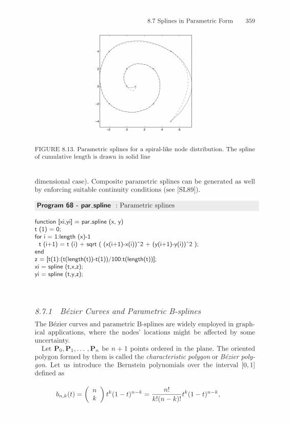
8.7 Splines in Parametric Form 359
!2 0 2 4 6
!4
!2
0
2
4
FIGURE 8.13. Parametric splines for a spiral-like node distribution. The splineof cumulative length is drawn in solid line
dimensional case). Composite parametric splines can be generated as wellby enforcing suitable continuity conditions (see [SL89]).
Program 68 - par spline : Parametric splines
function [xi,yi] = par spline (x, y)t (1) = 0;for i = 1:length (x)-1t (i+1) = t (i) + sqrt ( (x(i+1)-x(i))ˆ2 + (y(i+1)-y(i))ˆ2 );
endz = [t(1):(t(length(t))-t(1))/100:t(length(t))];xi = spline (t,x,z);yi = spline (t,y,z);
8.7.1 Bezier Curves and Parametric B-splinesThe Bezier curves and parametric B-splines are widely employed in graph-ical applications, where the nodes’ locations might be a!ected by someuncertainty.
Let P0,P1, . . . ,Pn be n + 1 points ordered in the plane. The orientedpolygon formed by them is called the characteristic polygon or Bezier poly-gon. Let us introduce the Bernstein polynomials over the interval [0, 1]defined as
bn,k(t) =4
nk
5tk(1" t)n"k =
n!k!(n" k)!
tk(1" t)n"k,

360 8. Polynomial Interpolation
for n = 0, 1, . . . and k = 0, . . . , n. They can be obtained by the followingrecursive formulaB
bn,0(t) = (1" t)n
bn,k(t) = (1" t)bn"1,k(t) + tbn"1,k"1(t), k = 1, . . . , n, t ! [0, 1].
It is easily seen that bn,k ! Pn, for k = 0, . . . , n. Also, {bn,k, k = 0, . . . , n}provides a basis for Pn. The Bezier curve is defined as follows
Bn(P0,P1, . . . ,Pn, t) =n(
k=0
Pkbn,k(t), 0 & t & 1. (8.58)
This expression can be regarded as a weighted average of the points Pk,with weights bn,k(t).
The Bezier curves can also be obtained by a pure geometric approachstarting from the characteristic polygon. Indeed, for any fixed t ! [0, 1],we define Pi,1(t) = (1 " t)Pi + tPi+1 for i = 0, . . . , n " 1 and, for tfixed, the piecewise line that joins the new nodes Pi,1(t) forms a polygonof n " 1 edges. We can now repeat the procedure by generating the newvertices Pi,2(t) (i = 0, . . . , n" 2), and terminating as soon as the polygoncomprises only the vertices P0,n"1(t) and P1,n"1(t). It can be shown that
P0,n(t) = (1" t)P0,n"1(t) + tP1,n"1(t) = Bn(P0,P1, . . . ,Pn, t),
that is, P0,n(t) is equal to the value of the Bezier curve Bn at the pointscorresponding to the fixed value of t. Repeating the process for several val-ues of the parameter t yields the construction of the curve in the consideredregion of the plane.
2 4 6 8 10 12 14 16!4
!2
0
2
4
6
8
FIGURE 8.14. Computation of the value of B3 relative to the points (0,0), (4,7),(14,7), (17,0) for t = 0.5, using the graphical method described in the text
Notice that, for a given node configuration, several curves can be con-structed according to the ordering of points Pi. Moreover, the Bezier curve
8.7 Splines in Parametric Form 361
Bn(P0,P1, . . . ,Pn, t) coincides with Bn(Pn,Pn"1, . . . ,P0, t), apart fromthe orientation.
Program 69 computes bn,k at the point x for x ! [0, 1].
Program 69 - bernstein : Bernstein polynomials
function [bnk]=bernstein (n,k,x)if k == 0,
C = 1;else,
C = prod ([1:n])/( prod([1:k])*prod([1:n-k]));endbnk = C * xˆk * (1-x)ˆ(n-k);
Program 70 plots the Bezier curve relative to the set of points (x, y).
Program 70 - bezier : Bezier curves
function [bezx,bezy] = bezier (x, y, n)i = 0; k = 0;for t = 0:0.01:1,
i = i + 1; bnk = bernstein (n,k,t); ber(i) = bnk;endbezx = ber * x (1); bezy = ber * y (1);for k = 1:n
i = 0;for t = 0:0.01:1
i = i + 1; bnk = bernstein (n,k,t); ber(i) = bnk;end
bezx = bezx + ber * x (k+1); bezy = bezy + ber * y (k+1);endplot(bezx,bezy)
In practice, the Bezier curves are rarely used since they do not provide asu"ciently accurate approximation to the characteristic polygon. For thisreason, in the 70’s the parametric B-splines were introduced, and they areused in (8.58) instead of the Bernstein polynomials. Parametric B-splinesare widely employed in packages for computer graphics since they enjoythe following properties:
1. perturbing a single vertex of the characteristic polygon yields a localperturbation of the curve only around the vertex itself;
2. the parametric B-spline better approximates the control polygon thanthe corresponding Bezier curve does, and it is always contained withinthe convex hull of the polygon.

362 8. Polynomial Interpolation
In Figure 8.15 a comparison is made between Bezier curves and para-metric B-splines for the approximation of a given characteristic polygon.
FIGURE 8.15. Comparison of a Bezier curve (left) and a parametric B-spline(right). The vertices of the characteristic polygon are denoted by 1
We conclude this section by noticing that parametric cubic B-splinesallow for obtaining locally straight lines by aligning four consecutive ver-tices (see Figure 8.16) and that a parametric B-spline can be constrainedat a specific point of the characteristic polygon by simply making threeconsecutive points of the polygon coincide with the desired point.
FIGURE 8.16. Some parametric B-splines as functions of the number and posi-tions of the vertices of the characteristic polygon. Notice in the last figure (right)the localization e"ects due to moving a single vertex
8.8 Applications
In this section we consider two problems arising from the solution of fourth-order di!erential equations and from the reconstruction of images in axialtomographies.
8.8 Applications 363
8.8.1 Finite Element Analysis of a Clamped BeamLet us employ piecewise Hermite polynomials (see Section 8.4) for the nu-merical approximation of the transversal bending of a clamped beam. Thisproblem was already considered in Section 4.7.2 where centered finite dif-ferences were used.
The mathematical model is the fourth-order boundary value problem(4.74), here presented in the following general formulation
B("(x)u**(x))** = f(x), 0 < x < L
u(0) = u(L) = 0, u*(0) = u*(L) = 0.(8.59)
In the particular case of (4.74) we have " = EJ and f = P ; we assumehenceforth that " is a positive and bounded function over (0,L) and thatf ! L2(0,L).
We multiply (8.59) by a su"ciently smooth arbitrary function v, then,we integrate by parts twice, to obtain
L
0
"u**v**dx" ["u***v]L0 + ["u**v*]L0 =L
0
fvdx.
Problem (8.59) is then replaced by the following problem in integral form
findu ! V such thatL
0
"u**v**dx =L
0
fvdx, #v ! V, (8.60)
where
V =Rv : v(k) ! L2(0,L), k = 0, 1, 2, v(k)(0) = v(k)(L) = 0, k = 0, 1
S.
Problem (8.60) admits a unique solution, which represents the deformedconfiguration that minimizes the total potential energy of the beam overthe space V (see, for instance, [Red86], p. 156)
J(u) =L
0
412"(u**)2 " fu
5dx.
In view of the numerical solution of problem (8.60), we introduce a partitionTh of [0,L] into K subintervals Tk = [xk"1, xk], (k = 1, . . . ,K) of uniformlength h = L/K, with xk = kh, and the finite dimensional space
Vh =/vh ! C1([0,L]), vh|T ! P3(T )
#T ! Th, v(k)h (0) = v(k)
h (L) = 0, k = 0, 1S.
(8.61)

364 8. Polynomial Interpolation
Let us equip Vh with a basis. For this purpose, we associate with eachinternal node xi (i = 1, . . . ,K " 1) a support (i = Ti 2 Ti+1 and twofunctions 1i, 6i defined as follows: for any k, 1i|Tk ! P3(Tk), 6i|Tk ! P3(Tk)and for any j = 0, . . . ,K,
)+
,
1i(xj) = %ij , 1*i(xj) = 0,
6i(xj) = 0, 6*i(xj) = %ij .
(8.62)
Notice that the above functions belong to Vh and define a basis
Bh = {1i, 6i, i = 1, . . . ,K " 1}. (8.63)
These basis functions can be brought back to the reference interval T =[0, 1] for 0 & x & 1, by the a"ne maps x = hx + xk"1 between T and Tk,for k = 1, . . . ,K.
Therefore, let us introduce on the interval T the basis functions 1(0)0
and 1(1)0 , associated with the node x = 0, and 1(0)
1 and 1(1)1 , associated
with node x = 1. Each of these is of the form 1 = a0 + a1x + a2x2 +a3x3; in particular, the functions with superscript “0” must satisfy thefirst two conditions in (8.62), while those with superscript “1” must fulfillthe remaining two conditions. Solving the (4%4) associated system, we get
1(0)0 (x) = 1" 3x2 + 2x3, 1(1)
0 (x) = x" 2x2 + x3,
1(0)1 (x) = 3x2 " 2x3, 1(1)
1 (x) = "x2 + x3.(8.64)
The graphs of the functions (8.64) are drawn in Figure 8.17 (left), where(0), (1), (2) and (3) denote 1(0)
0 , 1(0)1 , 1(1)
0 and 1(1)1 , respectively.
The function uh ! Vh can be written as
uh(x) =K"1(
i=1
ui1i(x) +K"1(
i=1
u(1)i 6i(x). (8.65)
The coe"cients and the degrees of freedom of uh have the following mean-ing: ui = uh(xi), u
(1)i (xi) = u*
h(xi) for i = 1, . . . ,K " 1. Notice that (8.65)is a special instance of (8.32), having set mi = 1.
The discretization of problem (8.60) reads
finduh ! Vh such thatL
0
"u**hv
**hdx =
L
0
fvhdx, #vh ! Bh. (8.66)
This is called the Galerkin finite element approximation of the di!erentialproblem (8.59). We refer to Chapter 12, Sections 12.4 and 12.4.5, for amore comprehensive discussion and analysis of the method.

8.8 Applications 365
0 0.2 0.4 0.6 0.8 1!0.2
0
0.2
0.4
0.6
0.8
1
(0) (1)
(2)
(3)
0 20 40 60 80 100 120 140 16010
!20
10!15
10!10
10!5
100
105
No Prec.Prec.
FIGURE 8.17. Canonical Hermite basis on the reference interval 0 " x " 1 (left);convergence histories for the conjugate gradient method in the solution of system(8.69) (right). On the x-axis the number of iterations k is shown, while the y-axisrepresents the quantity &r(k)&2/&b1&2, where r is the residual of system (8.69)
Using the representation (8.65) we end up with the following system inthe 2K " 2 unknowns u1, u2, . . . , uK"1, u
(1)1 , u(1)
2 , . . . u(1)K"1
)******+
******,
K"1(
j=1
)+
,uj
L
0
"1**j1
**i dx + u(1)
j
L
0
"6**j 1
**i dx
_`
a =L
0
f1idx,
K"1(
j=1
)+
,uj
L
0
"1**j6
**i dx + u(1)
j
L
0
"6**j 6
**i dx
_`
a =L
0
f6idx,
(8.67)
for i = 1, . . . ,K"1. Assuming, for the sake of simplicity, that the beam hasunit length L, that " and f are two constants and computing the integralsin (8.67), the final system reads in matrix form
BAu + Bp = b1
BTu + Cp = 0,(8.68)
where the vectors u,p ! RK"1 contain the nodal unknowns ui and u(1)i ,
b1 ! RK"1 is the vector of components equal to h4f/", while
A = tridiagK"1("12, 24,"12),
B = tridiagK"1("6, 0, 6),
C = tridiagK"1(2, 8, 2).
System (8.68) has size equal to 2(K " 1); eliminating the unknown p fromthe second equation, we get the reduced system (of size K " 1)
8A" BC"1BT
9u = b1. (8.69)
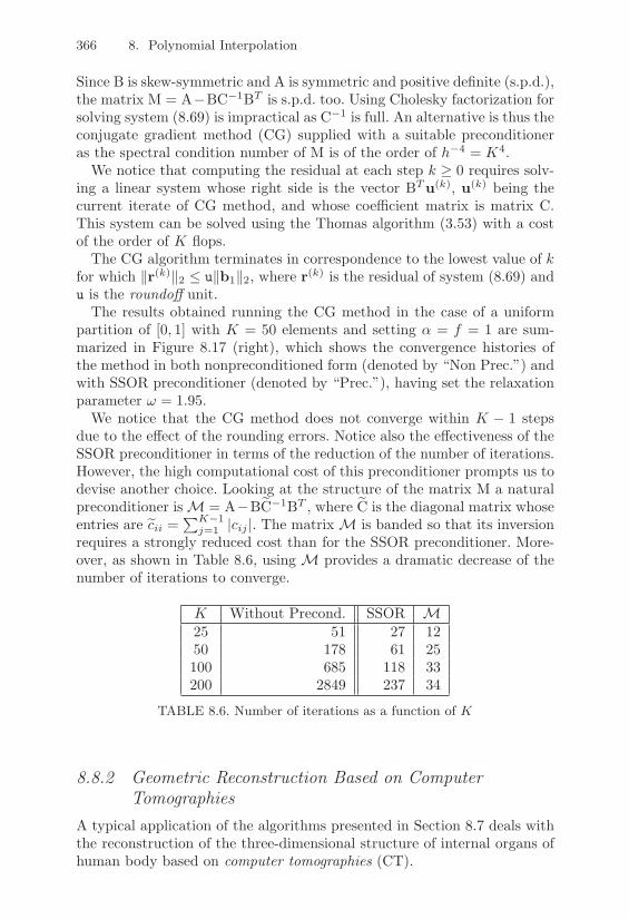
366 8. Polynomial Interpolation
Since B is skew-symmetric and A is symmetric and positive definite (s.p.d.),the matrix M = A"BC"1BT is s.p.d. too. Using Cholesky factorization forsolving system (8.69) is impractical as C"1 is full. An alternative is thus theconjugate gradient method (CG) supplied with a suitable preconditioneras the spectral condition number of M is of the order of h"4 = K4.
We notice that computing the residual at each step k ) 0 requires solv-ing a linear system whose right side is the vector BTu(k), u(k) being thecurrent iterate of CG method, and whose coe"cient matrix is matrix C.This system can be solved using the Thomas algorithm (3.53) with a costof the order of K flops.
The CG algorithm terminates in correspondence to the lowest value of kfor which +r(k)+2 & u+b1+2, where r(k) is the residual of system (8.69) andu is the roundo! unit.
The results obtained running the CG method in the case of a uniformpartition of [0, 1] with K = 50 elements and setting " = f = 1 are sum-marized in Figure 8.17 (right), which shows the convergence histories ofthe method in both nonpreconditioned form (denoted by “Non Prec.”) andwith SSOR preconditioner (denoted by “Prec.”), having set the relaxationparameter 0 = 1.95.
We notice that the CG method does not converge within K " 1 stepsdue to the e!ect of the rounding errors. Notice also the e!ectiveness of theSSOR preconditioner in terms of the reduction of the number of iterations.However, the high computational cost of this preconditioner prompts us todevise another choice. Looking at the structure of the matrix M a naturalpreconditioner is M = A"BDC"1BT , where DC is the diagonal matrix whoseentries are Dcii =
!K"1j=1 |cij |. The matrix M is banded so that its inversion
requires a strongly reduced cost than for the SSOR preconditioner. More-over, as shown in Table 8.6, using M provides a dramatic decrease of thenumber of iterations to converge.
K Without Precond. SSOR M25 51 27 1250 178 61 25100 685 118 33200 2849 237 34
TABLE 8.6. Number of iterations as a function of K
8.8.2 Geometric Reconstruction Based on ComputerTomographies
A typical application of the algorithms presented in Section 8.7 deals withthe reconstruction of the three-dimensional structure of internal organs ofhuman body based on computer tomographies (CT).

8.8 Applications 367
FIGURE 8.18. Cross-section of a blood vessel (left) and an associated character-istic polygon using 16 points Pi (right)
The CT usually provides a sequence of images which represent the sectionsof an organ at several horizontal planes; as a convention, we say that theCT produces sections of the x, y plane in correspondance of several values ofz. The result is analogous to what we would get by sectioning the organ atdi!erent values of z and taking the picture of the corresponding sections.Obviously, the great advantage in using the CT is that the organ underinvestigation can be visualized without being hidden by the neighboringones, as happens in other kinds of medical images, e.g., angiographies.
The image that is obtained for each section is coded into a matrix ofpixels (abbreviation of pictures elements) in the x, y plane; a certain valueis associated with each pixel expressing the level of grey of the image atthat point. This level is determined by the density of X rays which arecollected by a detector after passing through the human body. In practice,the information contained in a CT at a given value of z is expressed by aset of points (xi, yi) which identify the boundary of the organ at z.
To improve the diagnostics it is often useful to reconstruct the three-dimensional structure of the organ under examination starting from thesections provided by the CT. With this aim, it is necessary to convert theinformation coded by pixels into a parametric representation which can beexpressed by suitable functions interpolating the image at some significantpoints on its boundary. This reconstruction can be carried out by using themethods described in Section 8.7 as shown in Figure 8.19.A set of curves like those shown in Figure 8.19 can be suitably stacked toprovide an overall three-dimensional view of the organ under examination.
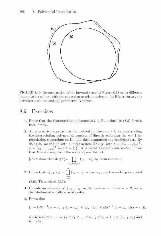
368 8. Polynomial Interpolation
(a)
(b)
(c)
FIGURE 8.19. Reconstruction of the internal vessel of Figure 8.18 using di"erentinterpolating splines with the same characteristic polygon: (a) Bezier curves, (b)parametric splines and (c) parametric B-splines
8.9 Exercises1. Prove that the characteristic polynomials li / Pn defined in (8.3) form a
basis for Pn.
2. An alternative approach to the method in Theorem 8.1, for constructingthe interpolating polynomial, consists of directly enforcing the n + 1 in-terpolation constraints on (n and then computing the coe!cients ai. Bydoing so, we end up with a linear system Xa= y, with a = (a0, . . . , an)T ,y = (y0, . . . , yn)T and X = [xj
i ]. X is called Vandermonde matrix. Provethat X is nonsingular if the nodes xi are distinct.
[Hint: show that det(X)=1
0*j<i*n
(xi % xj) by recursion on n.]
3. Prove that -(n+1(xi) =
n1
j=0j &=i
(xi % xj) where -n+1 is the nodal polynomial
(8.6). Then, check (8.5).
4. Provide an estimate of &-n+1&!, in the cases n = 1 and n = 2, for adistribution of equally spaced nodes.
5. Prove that
(n% 1)!hn%1|(x% xn%1)(x% xn)| " |-n+1(x)| " n!hn%1|(x% xn%1)(x% xn)|,
where n is even, %1 = x0 < x1 < . . . < xn%1 < xn = 1, x / (xn%1, xn) andh = 2/n.

8.9 Exercises 369
[Hint : let N = n/2 and show first that
-n+1(x) = (x + Nh)(x + (N % 1)h) . . . (x + h)x
(x% h) . . . (x% (N % 1)h)(x%Nh).(8.70)
Then, take x = rh with N % 1 < r < N .]
6. Under the assumptions of Exercise 5, show that |-n+1| is maximum ifx / (xn%1, xn) (notice that |-n+1| is an even function).[Hint : use (8.70) to prove that |-n+1(x + h)/-n+1(x)| > 1 for any x /(0, xn%1) with x not coinciding with any interpolation node.]
7. Prove the recursive relation (8.19) for Newton divided di"erences.
8. Determine an interpolating polynomial Hf / Pn such that
(Hf)(k)(x0) = f (k)(x0), k = 0, . . . , n,
and check that
Hf(x) =n(
j=0
f (j)(x0)j!
(x% x0)j ,
that is, the Hermite interpolating polynomial on one node coincides withthe Taylor polynomial.
9. Given the following set of data/f0 = f(%1) = 1, f1 = f ((%1) = 1, f2 = f ((1) = 2, f3 = f(2) = 1
0,
prove that the Hermite-Birko" interpolating polynomial H3 does not existfor them.[Solution : letting H3(x) = a3x
3 + a2x2 + a1x + a0, one must check that
the matrix of the linear system H3(xi) = fi for i = 0, . . . , 3 is singular.]
10. Check that any sk / Sk[a, b] admits a representation of the form
sk(x) =k(
i=0
bixi +
g(
i=1
ci(x% xi)k+,
that is, 1, x, x2, . . . , xk, (x% x1)k+, . . . , (x% xg)k+ form a basis for Sk[a, b].
11. Prove Property 8.2 and check its validity even in the case where the splines satisfies conditions of the form s((a) = f ((a), s((b) = f ((b).[Hint: start from
b^
a
Pf (((x)% s(((x)
Qs(((x)dx =
n(
i=1
xi^
xi"1
Pf (((x)% s(((x)
Qs((dx
and integrate by parts twice.]

370 8. Polynomial Interpolation
12. Let f(x) = cos(x) = 1 % x2
2! + x4
4! %x6
6! + . . . ; then, consider the followingrational approximation
r(x) =a0 + a2x
2 + a4x4
1 + b2x2 , (8.71)
called the Pade approximation. Determine the coe!cients of r in such away that
f(x)% r(x) = ,8x8 + ,10x
10 + . . .
[Solution: a0 = 1, a2 = %7/15, a4 = 1/40, b2 = 1/30.]
13. Assume that the function f of the previous exercise is known at a set of nequally spaced points xi / (%+/2,+/2) with i = 0, . . . , n. Repeat Exercise12, determining, by using MATLAB, the coe!cients of r in such a waythat the quantity
!ni=0 |f(xi) % r(xi)|2 is minimized. Consider the cases
n = 5 and n = 10.

9Numerical Integration
In this chapter we present the most commonly used methods for numer-ical integration. We will mainly consider one-dimensional integrals overbounded intervals, although in Sections 9.8 and 9.9 an extension of the tech-niques to integration over unbounded intervals (or integration of functionswith singularities) and to the multidimensional case will be considered.
9.1 Quadrature Formulae
Let f be a real integrable function over the interval [a, b]. Computing ex-plicitly the definite integral I(f) =
@ ba f(x)dx may be di"cult or even
impossible. Any explicit formula that is suitable for providing an approxi-mation of I(f) is said to be a quadrature formula or numerical integrationformula.
An example can be obtained by replacing f with an approximation fn,depending on the integer n ) 0, then computing I(fn) instead of I(f).Letting In(f) = I(fn), we have
In(f) =b^
a
fn(x)dx, n ) 0. (9.1)
The dependence on the end points a, b is always understood, so we writeIn(f) instead of In(f ; a, b).
372 9. Numerical Integration
If f ! C0([a, b]), the quadrature error En(f) = I(f)" In(f) satisfies
|En(f)| &b^
a
|f(x)" fn(x)|dx & (b" a)+f " fn+$.
Therefore, if for some n, +f " fn+$ < +, then |En(f)| & +(b" a).The approximant fn must be easily integrable, which is the case if, for
example, fn ! Pn. In this respect, a natural approach consists of usingfn = $nf , the interpolating Lagrange polynomial of f over a set of n + 1distinct nodes {xi}, with i = 0, . . . , n. By doing so, from (9.1) it followsthat
In(f) =n(
i=0
f(xi)b^
a
li(x)dx, (9.2)
where li is the characteristic Lagrange polynomial of degree n associatedwith node xi (see Section 8.1). We notice that (9.2) is a special instance ofthe following quadrature formula
In(f) =n(
i=0
"if(xi), (9.3)
where the coe"cients "i of the linear combination are given by@ ba li(x)dx.
Formula (9.3) is a weighted sum of the values of f at the points xi, fori = 0, . . . , n. These points are said to be the nodes of the quadratureformula, while the numbers "i ! R are its coe"cients or weights. Bothweights and nodes depend in general on n; again, for notational simplicity,this dependence is always understood.Formula (9.2), called the Lagrange quadrature formula, can be generalizedto the case where also the values of the derivative of f are available. Thisleads to the Hermite quadrature formula (see Section 9.5)
In(f) =1(
k=0
n(
i=0
"ikf(k)(xi) (9.4)
where the weights are now denoted by "ik.Both (9.2) and (9.4) are interpolatory quadrature formulae, since the
function f has been replaced by its interpolating polynomial (Lagrangeand Hermite polynomials, respectively). We define the degree of exactnessof a quadrature formula as the maximum integer r ) 0 for which
In(f) = I(f), #f ! Pr.
Any interpolatory quadrature formula that makes use of n + 1 distinctnodes has degree of exactness equal to at least n. Indeed, if f ! Pn, then
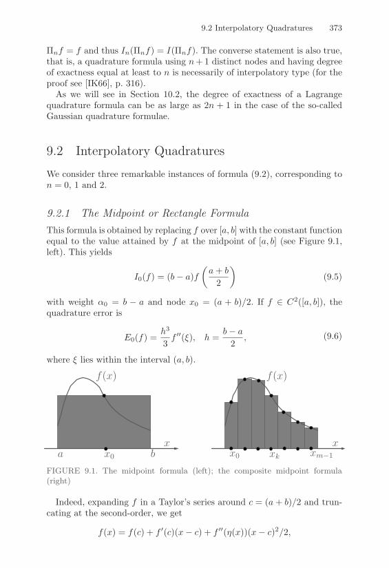
9.2 Interpolatory Quadratures 373
$nf = f and thus In($nf) = I($nf). The converse statement is also true,that is, a quadrature formula using n+ 1 distinct nodes and having degreeof exactness equal at least to n is necessarily of interpolatory type (for theproof see [IK66], p. 316).
As we will see in Section 10.2, the degree of exactness of a Lagrangequadrature formula can be as large as 2n + 1 in the case of the so-calledGaussian quadrature formulae.
9.2 Interpolatory Quadratures
We consider three remarkable instances of formula (9.2), corresponding ton = 0, 1 and 2.
9.2.1 The Midpoint or Rectangle FormulaThis formula is obtained by replacing f over [a, b] with the constant functionequal to the value attained by f at the midpoint of [a, b] (see Figure 9.1,left). This yields
I0(f) = (b" a)f4a + b
2
5(9.5)
with weight "0 = b " a and node x0 = (a + b)/2. If f ! C2([a, b]), thequadrature error is
E0(f) =h3
3f **(*), h =
b" a
2, (9.6)
where * lies within the interval (a, b).
ba
f(x)
x0
x
f(x)
xm!1xk
xx0
FIGURE 9.1. The midpoint formula (left); the composite midpoint formula(right)
Indeed, expanding f in a Taylor’s series around c = (a + b)/2 and trun-cating at the second-order, we get
f(x) = f(c) + f *(c)(x" c) + f **(-(x))(x" c)2/2,

374 9. Numerical Integration
from which, integrating on (a, b) and using the mean-value theorem, (9.6)follows. From this, it turns out that (9.5) is exact for constant and a"nefunctions (since in both cases f **(*) = 0 for any * ! (a, b)), so that themidpoint rule has degree of exactness equal to 1.It is worth noting that if the width of the integration interval [a, b] isnot su"ciently small, the quadrature error (9.6) can be quite large. Thisdrawback is common to all the numerical integration formulae that willbe described in the three forthcoming sections and can be overcome byresorting to their composite counterparts as discussed in Section 9.4.
Suppose now that we approximate the integral I(f) by replacing f over[a, b] with its composite interpolating polynomial of degree zero, constructedon m subintervals of width H = (b " a)/m, for m ) 1 (see Figure 9.1,right). Introducing the quadrature nodes xk = a + (2k + 1)H/2, for k =0, . . . ,m" 1, we get the composite midpoint formula
I0,m(f) = Hm"1(
k=0
f(xk), m ) 1. (9.7)
The quadrature error E0,m(f) = I(f)" I0,m(f) is given by
E0,m(f) =b" a
24H2f **(*), H =
b" a
m(9.8)
provided that f ! C2([a, b]) and where * ! (a, b). From (9.8) we concludethat (9.7) has degree of exactness equal to 1; (9.8) can be proved by recalling(9.6) and using the additivity of integrals. Indeed, for k = 0, . . . ,m"1 and*k ! (a + kH, a + (k + 1)H),
E0,m(f) =m"1(
k=0
f **(*k)(H/2)3/3 =m"1(
k=0
f **(*k)H2
24b" a
m=
b" a
24H2f **(*).
The last equality is a consequence of the following theorem, that is appliedletting u = f ** and %j = 1 for j = 0, . . . ,m" 1.
Theorem 9.1 (discrete mean-value theorem) Let u ! C0([a, b]) andlet xj be s+1 points in [a, b] and %j be s+1 constants, all having the samesign. Then there exists - ! [a, b] such that
s(
j=0
%ju(xj) = u(-)s(
j=0
%j . (9.9)
Proof. Let um = minx'[a,b] u(x) = u(x) and uM = maxx'[a,b] u(x) = u(¯x),where x and ¯x are two points in (a, b). Then
um
s(
j=0
!j "s(
j=0
!ju(xj) " uM
s(
j=0
!j . (9.10)
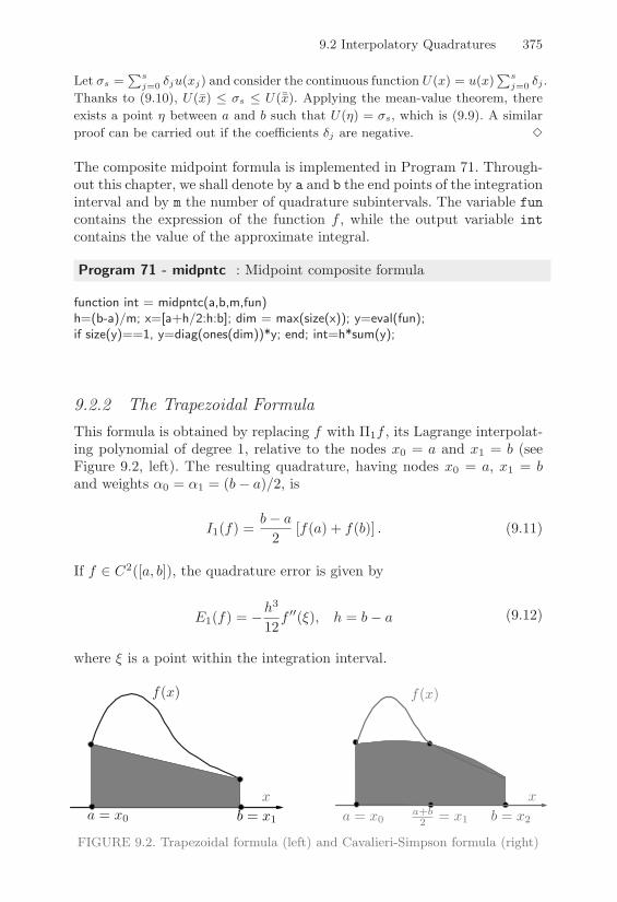
9.2 Interpolatory Quadratures 375
Let 's =!s
j=0 !ju(xj) and consider the continuous function U(x) = u(x)!s
j=0 !j .Thanks to (9.10), U(x) " 's " U(¯x). Applying the mean-value theorem, thereexists a point 0 between a and b such that U(0) = 's, which is (9.9). A similarproof can be carried out if the coe!cients !j are negative. !
The composite midpoint formula is implemented in Program 71. Through-out this chapter, we shall denote by a and b the end points of the integrationinterval and by m the number of quadrature subintervals. The variable funcontains the expression of the function f , while the output variable intcontains the value of the approximate integral.
Program 71 - midpntc : Midpoint composite formula
function int = midpntc(a,b,m,fun)h=(b-a)/m; x=[a+h/2:h:b]; dim = max(size(x)); y=eval(fun);if size(y)==1, y=diag(ones(dim))*y; end; int=h*sum(y);
9.2.2 The Trapezoidal FormulaThis formula is obtained by replacing f with $1f , its Lagrange interpolat-ing polynomial of degree 1, relative to the nodes x0 = a and x1 = b (seeFigure 9.2, left). The resulting quadrature, having nodes x0 = a, x1 = band weights "0 = "1 = (b" a)/2, is
I1(f) =b" a
2[f(a) + f(b)] . (9.11)
If f ! C2([a, b]), the quadrature error is given by
E1(f) = "h3
12f **(*), h = b" a (9.12)
where * is a point within the integration interval.
f(x)
a = x0 b = x1
x
b = x2a+b2 = x1
x
f(x)
a = x0
FIGURE 9.2. Trapezoidal formula (left) and Cavalieri-Simpson formula (right)

376 9. Numerical Integration
Indeed, from the expression of the interpolation error (8.7) one gets
E1(f) =b^
a
(f(x)"$1f(x))dx = "12
b^
a
f **(*(x))(x" a)(b" x)dx.
Since 02(x) = (x" a)(x" b) < 0 in (a, b), the mean-value theorem yields
E1(f) = (1/2)f **(*)b^
a
02(x)dx = "f **(*)(b" a)3/12,
for some * ! (a, b), which is (9.12). The trapezoidal quadrature thereforehas degree of exactness equal to 1, as is the case with the midpoint rule.
To obtain the composite trapezoidal formula, we proceed as in the casewhere n = 0, by replacing f over [a, b] with its composite Lagrange polyno-mial of degree 1 on m subintervals, with m ) 1. Introduce the quadraturenodes xk = a + kH, for k = 0, . . . ,m and H = (b" a)/m, getting
I1,m(f) =H
2
m"1(
k=0
(f(xk) + f(xk+1)) , m ) 1. (9.13)
Each term in (9.13) is counted twice, except the first and the last one, sothat the formula can be written as
I1,m(f) = H
-12f(x0) + f(x1) + . . . + f(xm"1) +
12f(xm)
.. (9.14)
As was done for (9.8), it can be shown that the quadrature error associatedwith (9.14) is
E1,m(f) = "b" a
12H2f **(*),
provided that f ! C2([a, b]), where * ! (a, b). The degree of exactness isagain equal to 1.
The composite trapezoidal rule is implemented in Program 72.
Program 72 - trapezc : Composite trapezoidal formula
function int = trapezc(a,b,m,fun)h=(b-a)/m; x=[a:h:b]; dim = max(size(x)); y=eval(fun);if size(y)==1, y=diag(ones(dim))*y; end;int=h*(0.5*y(1)+sum(y(2:m))+0.5*y(m+1));

9.2 Interpolatory Quadratures 377
9.2.3 The Cavalieri-Simpson FormulaThe Cavalieri-Simpson formula can be obtained by replacing f over [a, b]with its interpolating polynomial of degree 2 at the nodes x0 = a, x1 =(a + b)/2 and x2 = b (see Figure 9.2, right). The weights are given by"0 = "2 = (b" a)/6 and "1 = 4(b" a)/6, and the resulting formula reads
I2(f) =b" a
6
-f(a) + 4f
4a + b
2
5+ f(b)
.. (9.15)
It can be shown that the quadrature error is
E2(f) = "h5
90f (4)(*), h =
b" a
2(9.16)
provided that f ! C4([a, b]), and where * lies within (a, b). From (9.16) itturns out that (9.15) has degree of exactness equal to 3.
Replacing f with its composite polynomial of degree 2 over [a, b] yieldsthe composite formula corresponding to (9.15). Introducing the quadraturenodes xk = a + kH/2, for k = 0, . . . , 2m and letting H = (b" a)/m, withm ) 1 gives
I2,m =H
6
N
f(x0) + 2m"1(
r=1
f(x2r) + 4m"1(
s=0
f(x2s+1) + f(x2m)
O
. (9.17)
The quadrature error associated with (9.17) is
E2,m(f) = "b" a
180(H/2)4f (4)(*),
provided that f ! C4([a, b]) and where * ! (a, b); the degree of exactnessof the formula is 3.The composite Cavalieri-Simpson quadrature is implemented in Program73.
Program 73 - simpsonc : Composite Cavalieri-Simpson formula
function int = simpsonc(a,b,m,fun)h=(b-a)/m; x=[a:h/2:b]; dim = max(size(x)); y=eval(fun);if size(y)==1, y=diag(ones(dim))*y; end;int=(h/6)*(y(1)+2*sum(y(3:2:2*m-1))+4*sum(y(2:2:2*m))+y(2*m+1));
Example 9.1 Let us employ the midpoint, trapezoidal and Cavalieri-Simpsoncomposite formulae to compute the integral
2)^
0
xe%x cos(2x)dx =P3(e%2) % 1)% 10+e%2)
Q
250 %0.122122. (9.18)

378 9. Numerical Integration
Table 9.1 shows in even columns the behavior of the absolute value of the er-ror when halving H (thus, doubling m), while in odd columns the ratio Rm =|Em|/|E2m| between two consecutive errors is given. As predicted by the previoustheoretical analysis, Rm tends to 4 for the midpoint and trapezoidal rules andto 16 for the Cavalieri-Simpson formula. •
m |E0,m| Rm |E1,m| Rm |E2,m| Rm
1 0.9751 1.589e-01 7.030e-012 1.037 0.9406 0.5670 0.2804 0.5021 1.4004 0.1221 8.489 0.2348 2.415 3.139 · 10"3 159.968 2.980 · 10"2 4.097 5.635 · 10"2 4.167 1.085 · 10"3 2.89216 6.748 · 10"3 4.417 1.327 · 10"2 4.245 7.381 · 10"5 14.70432 1.639 · 10"3 4.118 3.263 · 10"3 4.068 4.682 · 10"6 15.76564 4.066 · 10"4 4.030 8.123 · 10"4 4.017 2.936 · 10"7 15.946128 1.014 · 10"4 4.008 2.028 · 10"4 4.004 1.836 · 10"8 15.987256 2.535 · 10"5 4.002 5.070 · 10"5 4.001 1.148 · 10"9 15.997
TABLE 9.1. Absolute error for midpoint, trapezoidal and Cavalieri-Simpson com-posite formulae in the approximate evaluation of integral (9.18)
9.3 Newton-Cotes Formulae
These formulae are based on Lagrange interpolation with equally spacednodes in [a, b]. For a fixed n ) 0, let us denote the quadrature nodesby xk = x0 + kh, k = 0, . . . , n. The midpoint, trapezoidal and Simpsonformulae are special instances of the Newton-Cotes formulae, taking n = 0,n = 1 and n = 2 respectively. In the general case, we define:
- closed formulae, those where x0 = a, xn = b and h =b" a
n(n ) 1);
- open formulae, those where x0 = a+h, xn = b"h and h =b" a
n + 2(n ) 0).
A significant property of the Newton-Cotes formulae is that the quadra-ture weights "i depend explicitly only on n and h, but not on the integrationinterval [a, b]. To check this property in the case of closed formulae, let usintroduce the change of variable x = )(t) = x0 + th. Noting that )(0) = a,)(n) = b and xk = a + kh, we get
x" xk
xi " xk=
a + th" (a + kh)a + ih" (a + kh)
=t" k
i" k.
Therefore, if n ) 1
li(x) =n1
k=0,k '=i
t" k
i" k= 1i(t), 0 & i & n.
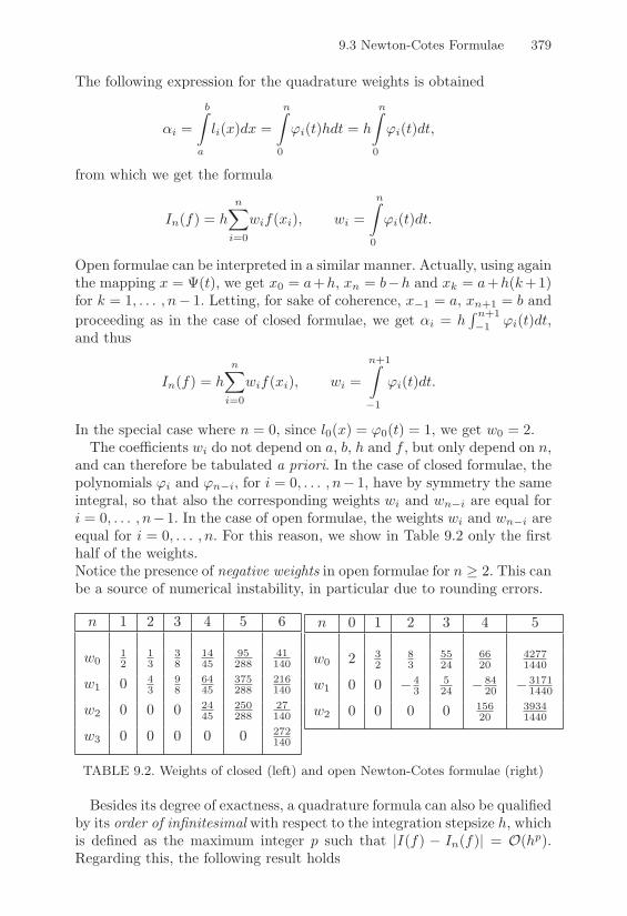
9.3 Newton-Cotes Formulae 379
The following expression for the quadrature weights is obtained
"i =b^
a
li(x)dx =n
0
1i(t)hdt = h
n
0
1i(t)dt,
from which we get the formula
In(f) = hn(
i=0
wif(xi), wi =n
0
1i(t)dt.
Open formulae can be interpreted in a similar manner. Actually, using againthe mapping x = )(t), we get x0 = a+h, xn = b"h and xk = a+h(k+1)for k = 1, . . . , n" 1. Letting, for sake of coherence, x"1 = a, xn+1 = b andproceeding as in the case of closed formulae, we get "i = h
@ n+1"1 1i(t)dt,
and thus
In(f) = hn(
i=0
wif(xi), wi =n+1^
"1
1i(t)dt.
In the special case where n = 0, since l0(x) = 10(t) = 1, we get w0 = 2.The coe"cients wi do not depend on a, b, h and f , but only depend on n,
and can therefore be tabulated a priori. In the case of closed formulae, thepolynomials 1i and 1n"i, for i = 0, . . . , n" 1, have by symmetry the sameintegral, so that also the corresponding weights wi and wn"i are equal fori = 0, . . . , n"1. In the case of open formulae, the weights wi and wn"i areequal for i = 0, . . . , n. For this reason, we show in Table 9.2 only the firsthalf of the weights.Notice the presence of negative weights in open formulae for n ) 2. This canbe a source of numerical instability, in particular due to rounding errors.
n 1 2 3 4 5 6
w012
13
38
1445
95288
41140
w1 0 43
98
6445
375288
216140
w2 0 0 0 2445
250288
27140
w3 0 0 0 0 0 272140
n 0 1 2 3 4 5
w0 2 32
83
5524
6620
42771440
w1 0 0 " 43
524 " 84
20 " 31711440
w2 0 0 0 0 15620
39341440
TABLE 9.2. Weights of closed (left) and open Newton-Cotes formulae (right)
Besides its degree of exactness, a quadrature formula can also be qualifiedby its order of infinitesimal with respect to the integration stepsize h, whichis defined as the maximum integer p such that |I(f) " In(f)| = O(hp).Regarding this, the following result holds

380 9. Numerical Integration
Theorem 9.2 For any Newton-Cotes formula corresponding to an evenvalue of n, the following error characterization holds
En(f) =Mn
(n + 2)!hn+3f (n+2)(*), (9.19)
provided f ! Cn+2([a, b]), where * ! (a, b) and
Mn =
)******+
******,
n
0
t &n+1(t)dt < 0 for closed formulae,
n+1^
"1
t &n+1(t)dt > 0 for open formulae,
having defined &n+1(t) =bn
i=0(t " i). From (9.19), it turns out that thedegree of exactness is equal to n+ 1 and the order of infinitesimal is n+ 3.
Similarly, for odd values of n, the following error characterization holds
En(f) =Kn
(n + 1)!hn+2f (n+1)(-), (9.20)
provided f ! Cn+1([a, b]), where - ! (a, b) and
Kn =
)******+
******,
n
0
&n+1(t)dt < 0 for closed formulae,
n+1^
"1
&n+1(t)dt > 0 for open formulae.
The degree of exactness is thus equal to n and the order of infinitesimal isn + 2.
Proof. We give a proof in the particular case of closed formulae with n even,referring to [IK66], pp. 308-314, for a complete demonstration of the theorem.
Thanks to (8.20), we have
En(f) = I(f)% In(f) =b^
a
f [x0, . . . , xn, x]-n+1(x)dx. (9.21)
Set W (x) =@ x
a-n+1(t)dt. Clearly, W (a) = 0; moreover, -n+1(t) is an odd func-
tion with respect to the midpoint (a + b)/2 so that W (b) = 0. Integrating by

9.3 Newton-Cotes Formulae 381
parts (9.21) we get
En(f) =b^
a
f [x0, . . . , xn, x]W ((x)dx = %b^
a
ddx
f [x0, . . . , xn, x]W (x)dx
= %b^
a
f (n+2)(/(x))(n + 2)!
W (x)dx.
In deriving the formula above we have used the following identity (see Exercise4)
ddx
f [x0, . . . , xn, x] = f [x0, . . . , xn, x, x]. (9.22)
Since W (x) > 0 for a < x < b (see [IK66], p. 309), using the mean-value theoremwe obtain
En(f) = %f (n+2)(/)(n + 2)!
b^
a
W (x)dx = %f (n+2)(/)(n + 2)!
b^
a
x^
a
-n+1(t) dt dx (9.23)
where / lies within (a, b). Exchanging the order of integration, letting s = x0+4h,for 0 " 4 " n, and recalling that a = x0, b = xn, yields
b^
a
W (x)dx =b^
a
b^
s
(s% x0) . . . (s% xn)dxds
=xn^
x0
(s% x0) . . . (s% xn%1)(s% xn)(xn % s)ds
= %hn+3
n^
0
4(4 % 1) . . . (4 % n + 1)(4 % n)2d4.
Finally, letting t = n% 4 and combining this result with (9.23), we get (9.19). !
Relations (9.19) and (9.20) are a priori estimates for the quadrature error(see Chapter 2, Section 2.3). Their use in generating a posteriori estimatesof the error in the frame of adaptive algorithms will be examined in Section9.7.
In the case of closed Newton-Cotes formulae, we show in Table 9.3, for1 & n & 6, the degree of exactness (that we denote henceforth by rn) andthe absolute value of the constant Mn = Mn/(n + 2)! (if n is even) orKn = Kn/(n + 1)! (if n is odd).
Example 9.2 The purpose of this example is to assess the importance of theregularity assumption on f for the error estimates (9.19) and (9.20). Considerthe closed Newton-Cotes formulae, for 1 " n " 6, to approximate the integral@ 10 x5/2dx = 2/7 0 0.2857. Since f is only C2([0, 1]), we do not expect a substan-
tial increase of the accuracy as n gets larger. Actually, this is confirmed by Table9.4, where the results obtained by running Program 74 are reported.
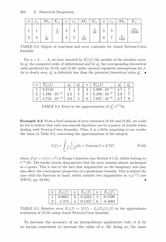
382 9. Numerical Integration
n rn Mn Kn n rn Mn Kn n rn Mn Kn
1 1 112 3 3 3
80 5 5 27512096
2 3 190 4 5 8
945 6 7 91400
TABLE 9.3. Degree of exactness and error constants for closed Newton-Cotesformulae
For n = 1, . . . , 6, we have denoted by Ecn(f) the module of the absolute error,
by qcn the computed order of infinitesimal and by qsn the corresponding theoreticalvalue predicted by (9.19) and (9.20) under optimal regularity assumptions for f .As is clearly seen, qcn is definitely less than the potential theoretical value qsn. •
n Ecn(f) qcn qsn n Ec
n(f) qcn qsn1 0.2143 3 3 4 5.009 · 10"5 4.7 72 1.196 · 10"3 3.2 5 5 3.189 · 10"5 2.6 73 5.753 · 10"4 3.8 5 6 7.857 · 10"6 3.7 9
TABLE 9.4. Error in the approximation of@ 10 x5/2dx
Example 9.3 From a brief analysis of error estimates (9.19) and (9.20), we couldbe led to believe that only non-smooth functions can be a source of trouble whendealing with Newton-Cotes formulae. Thus, it is a little surprising to see resultslike those in Table 9.5, concerning the approximation of the integral
I(f) =5^
%5
11 + x2 dx = 2arctan 5 0 2.747, (9.24)
where f(x) = 1/(1+x2) is Runge’s function (see Section 8.1.2), which belongs toC!(R). The results clearly demonstrate that the error remains almost unchangedas n grows. This is due to the fact that singularities on the imaginary axis mayalso a"ect the convergence properties of a quadrature formula. This is indeed thecase with the function at hand, which exhibits two singularities at ±
'%1 (see
[DR75], pp. 64-66). •
n En(f) n En(f) n En(f)1 0.8601 3 0.2422 5 0.15992 -1.474 4 0.1357 6 -0.4091
TABLE 9.5. Relative error En(f) = [I(f) % In(f)]/In(f) in the approximateevaluation of (9.24) using closed Newton-Cotes formulae
To increase the accuracy of an interpolatory quadrature rule, it is byno means convenient to increase the value of n. By doing so, the same

9.4 Composite Newton-Cotes Formulae 383
drawbacks of Lagrange interpolation on equally spaced nodes would arise.For example, the weights of the closed Newton-Cotes formula with n = 8do not have the same sign (see Table 9.6 and recall that wi = wn"i fori = 0, . . . , n" 1).
n w0 w1 w2 w3 w4 rn Mn
8 395614175
2355214175 " 3712
141754198414175 "18160
141759 2368
467775
TABLE 9.6. Weights of the closed Newton-Cotes formula with 9 nodes
This can give rise to numerical instabilities, due to rounding errors (seeChapter 2), and makes this formula useless in the practice, as happens forall the Newton-Cotes formulae using more than 8 nodes. As an alternative,one can resort to composite formulae, whose error analysis is addressed inSection 9.4, or to Gaussian formulae, which will be dealt with in Chapter10 and which yield maximum degree of exactness with a non equally spacednodes distribution.
The closed Newton-Cotes formulae, for 1 & n & 6, are implemented inProgram 74.
Program 74 - newtcot : Closed Newton-Cotes formulae
function int = newtcot(a,b,n,fun)h=(b-a)/n; n2=fix(n/2);if n > 6, disp(’maximum value of n equal to 6 ’); return; enda03=1/3; a08=1/8; a45=1/45; a288=1/288; a140=1/140;alpha=[0.5 0 0 0; ...
a03 4*a03 0 0; ...3*a08 9*a08 0 0; ...14*a45 64*a45 24*a45 0; ...95*a288 375*a288 250*a288 0; ...41*a140 216*a140 27*a140 272*a140];
x=a; y(1)=eval(fun);for j=2:n+1, x=x+h; y(j)=eval(f); end; int=0;for j=1:n2+1, int=int+y(j)*alpha(n,j); end;for j=n2+2:n+1, int=int+y(j)*alpha(n,n-j+2); end; int=int*h;
9.4 Composite Newton-Cotes Formulae
The examples of Section 9.2 have already pointed out that compositeNewton-Cotes formulae can be constructed by replacing f with its com-posite Lagrange interpolating polynomial, introduced in Section 8.1.

384 9. Numerical Integration
The general procedure consists of partitioning the integration interval[a, b] into m subintervals Tj = [yj , yj+1] such that yj = a+ jH, where H =(b " a)/m for j = 0, . . . ,m. Then, over each subinterval, an interpolatoryformula with nodes {x(j)
k , 0 & k & n} and weights {"(j)k , 0 & k & n} is
used. Since
I(f) =b^
a
f(x)dx =m"1(
j=0
^
Tj
f(x)dx,
a composite interpolatory quadrature formula is obtained by replacing I(f)with
In,m(f) =m"1(
j=0
n(
k=0
"(j)k f(x(j)
k ). (9.25)
The quadrature error is defined as En,m(f) = I(f)"In,m(f). In particular,over each subinterval Tj one can resort to a Newton-Cotes formula withn+ 1 equally spaced nodes: in such a case, the weights "(j)
k = hwk are stillindependent of Tj .
Using the same notation as in Theorem 9.2, the following convergenceresult holds for composite formulae.
Theorem 9.3 Let a composite Newton-Cotes formula, with n even, beused. If f ! Cn+2([a, b]), then
En,m(f) =b" a
(n + 2)!Mn
(n + 2)n+3Hn+2f (n+2)(*) (9.26)
where * ! (a, b). Therefore, the quadrature error is an infinitesimal in Hof order n + 2 and the formula has degree of exactness equal to n + 1.
For a composite Newton-Cotes formula, with n odd, if f ! Cn+1([a, b])
En,m(f) =b" a
(n + 1)!Kn
nn+2Hn+1f (n+1)(-) (9.27)
where - ! (a, b). Thus, the quadrature error is an infinitesimal in H oforder n + 1 and the formula has degree of exactness equal to n.
Proof. We only consider the case where n is even. Using (9.19), and noticingthat Mn does not depend on the integration interval, we get
En,m(f) =m%1(
j=0
PI(f)|Tj % In(f)|Tj
Q=
Mn
(n + 2)!
m%1(
j=0
hn+3j f (n+2)(/j),
where, for j = 0, . . . , (m% 1), hj = |Tj |/(n+ 2) = (b% a)/(m(n+ 2)); this time,/j is a suitable point of Tj . Since (b% a)/m = H, we obtain
En,m(f) =Mn
(n + 2)!b% a
m(n + 2)n+3Hn+2
m%1(
j=0
f (n+2)(/j),

9.4 Composite Newton-Cotes Formulae 385
from which, applying Theorem 9.1 with u(x) = f (n+2)(x) and !j = 1 for j =0, . . . ,m% 1, (9.26) immediately follows. A similar procedure can be followed toprove (9.27). !
We notice that, for n fixed, En,m(f) ( 0 as m ( , (i.e., as H ( 0).This ensures the convergence of the numerical integral to the exact valueI(f). We notice also that the degree of exactness of composite formulaecoincides with that of simple formulae, whereas its order of infinitesimal(with respect to H) is reduced by 1 with respect to the order of infinitesimal(in h) of simple formulae.In practical computations, it is convenient to resort to a local interpolationof low degree (typically n & 2, as done in Section 9.2), this leads to com-posite quadrature rules with positive weights, with a minimization of therounding errors.
Example 9.4 For the same integral (9.24) considered in Example 9.3, we showin Table 9.7 the behavior of the absolute error as a function of the number ofsubintervals m, in the case of the composite midpoint, trapezoidal and Cavalieri-Simpson formulae. Convergence of In,m(f) to I(f) as m increases can be clearlyobserved. Moreover, we notice that E0,m(f) 0 E1,m(f)/2 for m ! 32 (see Exer-cise 1).
m |E0,m| |E1,m| |E2,m|1 7.253 2.362 4.042 1.367 2.445 9.65 · 10"2
8 3.90 · 10"2 3.77 · 10"2 1.35 · 10"2
32 1.20 · 10"4 2.40 · 10"4 4.55 · 10"8
128 7.52 · 10"6 1.50 · 10"5 1.63 · 10"10
512 4.70 · 10"7 9.40 · 10"7 6.36 · 10"13
TABLE 9.7. Absolute error for composite quadratures in the computation of(9.24)
•
Convergence of In,m(f) to I(f) can be established under less stringentregularity assumptions on f than those required by Theorem 9.3. In thisregard, the following result holds (see for the proof [IK66], pp. 341-343).
Property 9.1 Let f ! C0([a, b]) and assume that the weights "(j)k in (9.25)
are nonnegative. Then
limm&$
In,m(f) =^ b
af(x)dx, #n ) 0.
Moreover >>>>>
^ b
af(x)dx" In,m(f)
>>>>> & 2(b" a)((f ;H),

386 9. Numerical Integration
where
((f ;H) = sup{|f(x)" f(y)|, x, y ! [a, b], x '= y, |x" y| & H}
is the module of continuity of function f .
9.5 Hermite Quadrature Formulae
Thus far we have considered quadrature formulae based on Lagrange inter-polation (simple or composite). More accurate formulae can be devised byresorting to Hermite interpolation (see Section 8.4).
Suppose that 2(n+1) values f(xk), f *(xk) are available at n+1 distinctpoints x0, . . . , xn, then the Hermite interpolating polynomial of f is givenby
H2n+1f(x) =n(
i=0
f(xi)Li(x) +n(
i=0
f *(xi)Mi(x), (9.28)
where the polynomials Lk,Mk ! P2n+1 are defined, for k = 0, . . . , n, as
Lk(x) =-1"
0**n+1(xk)0*n+1(xk)
(x" xk).l2k(x), Mk(x) = (x" xk)l2k(x).
Integrating (9.28) over [a, b], we get the quadrature formula of type (9.4)
In(f) =n(
k=0
"kf(xk) +n(
k=0
#kf*(xk) (9.29)
where
"k = I(Lk), #k = I(Mk), k = 0, . . . , n.
Formula (9.29) has degree of exactness equal to 2n + 1. Taking n = 1, theso-called corrected trapezoidal formula is obtained
Icorr1 (f) =b" a
2[f(a) + f(b)] +
(b" a)2
12[f *(a)" f *(b)] (9.30)
with weights "0 = "1 = (b"a)/2, #0 = (b"a)2/12 and #1 = "#0. Assumingf ! C4([a, b]), the quadrature error associated with (9.30) is
Ecorr1 (f) =
h5
720f (4)(*), h = b" a (9.31)
with * ! (a, b). Notice the increase of accuracy from O(h3) to O(h5) withrespect to the corresponding expression (9.12) (of the same order as the

9.6 Richardson Extrapolation 387
Cavalieri-Simpson formula (9.15)). The composite formula can be generatedin a similar manner
Icorr1,m (f) =b" a
m
E12
[f(x0) + f(xm)]
+f(x1) + . . . + f(xm"1)} +(b" a)2
12[f *(a)" f *(b)] ,
(9.32)
where the assumption that f ! C1([a, b]) gives rise to the cancellation ofthe first derivatives at the nodes xk, with k = 1, . . . ,m" 1.
Example 9.5 Let us check experimentally the error estimate (9.31) in the simple(m = 1) and composite (m > 1) cases, running Program 75 for the approximatecomputation of integral (9.18). Table 9.8 reports the behavior of the module ofthe absolute error as H is halved (that is, m is doubled) and the ratio Rm betweentwo consecutive errors. This ratio, as happens in the case of Cavalieri-Simpsonformula, tends to 16, demonstrating that formula (9.32) has order of infinitesimalequal to 4. Comparing Table 9.8 with the corresponding Table 9.1, we can alsonotice that |Ecorr
1,m (f)| 0 4|E2,m(f)| (see Exercise 9). •
m Ecorr1,m (f) Rm m Ecorr
1,m (f) Rm m Ecorr1,m (f) Rm
1 3.4813 8 4.4 · 10"3 6.1 64 1.1 · 10"6 15.9572 1.398 2.4 16 2.9 · 10"4 14.9 128 7.3 · 10"8 15.9904 2.72 · 10"2 51.4 32 1.8 · 10"5 15.8 256 4.5 · 10"9 15.997
TABLE 9.8. Absolute error for the corrected trapezoidal formula in the compu-tation of I(f) =
@ 2)
0 xe%x cos(2x)dx
The corrected composite trapezoidal quadrature is implemented in Pro-gram 75, where dfun contains the expression of the derivative of f .
Program 75 - trapmodc : Composite corrected trapezoidal formula
function int = trapmodc(a,b,m,fun,dfun)h=(b-a)/m; x=[a:h:b]; y=eval(fun);f1a=feval(dfun,a); f1b=feval(dfun,b);int=h*(0.5*y(1)+sum(y(2:m))+0.5*y(m+1))+(hˆ2/12)*(f1a-f1b);
9.6 Richardson Extrapolation
The Richardson extrapolation method is a procedure which combines severalapproximations of a certain quantity "0 in a smart way to yield a moreaccurate approximation of "0. More precisely, assume that a method isavailable to approximate "0 by a quantity A(h) that is computable for any

388 9. Numerical Integration
value of the parameter h '= 0. Moreover, assume that, for a suitable k ) 0,A(h) can be expanded as follows
A(h) = "0 + "1h + . . . + "khk + Rk+1(h), (9.33)
where |Rk+1(h)| & Ck+1hk+1. The constants Ck+1 and the coe"cients "i,for i = 0, . . . , k, are independent of h. Henceforth, "0 = limh&0 A(h).
Writing (9.33) with %h instead of h, for 0 < % < 1 (typically, % = 1/2),we get
A(%h) = "0 + "1(%h) + . . . + "k(%h)k + Rk+1(%h).
Subtracting (9.33) multiplied by % from this expression then yields
B(h) =A(%h)" %A(h)
1" % = "0 + D"2h2 + . . . + D"kh
k + DRk+1(h),
having defined, for k ) 2, D"i = "i(%i " %)/(1 " %), for i = 2, . . . , k andDRk+1(h) = [Rk+1(%h)" %Rk+1(h)] /(1" %).Notice that D"i '= 0 i! "i '= 0. In particular, if "1 '= 0, then A(h) is a first-order approximation of "0, while B(h) is at least second-order accurate.More generally, if A(h) is an approximation of "0 of order p, then thequantity B(h) = [A(%h)" %pA(h)] /(1 " %p) approximates "0 up to orderp + 1 (at least).Proceeding by induction, the following Richardson extrapolation algorithmis generated: setting n ) 0, h > 0 and % ! (0, 1), we construct the sequences
Am,0 = A(%mh), m = 0, . . . , n,
Am,q+1 =Am,q " %q+1Am"1,q
1" %q+1 , q = 0, . . . , n" 1,
m = q + 1, . . . , n,
(9.34)
which can be represented by the diagram below
A0,0>
A1,0 ( A1,1> >
A2,0 ( A2,1 ( A2,2> > >
A3,0 ( A3,1 ( A3,2 ( A3,3> > > >
.... . . . . . . . . . . .> > > >
An,0 ( An,1 ( An,2 ( An,3 . . . ( An,n
where the arrows indicate the way the terms which have been alreadycomputed contribute to the construction of the “new” ones.
The following result can be proved (see [Com95], Proposition 4.1).

9.6 Richardson Extrapolation 389
Property 9.2 For n ) 0 and % ! (0, 1)
Am,n = "0 + O((%mh)n+1), m = 0, . . . , n. (9.35)
In particular, for the terms in the first column (n = 0) the convergencerate to "0 is O((%mh)), while for those of the last one it is O((%mh)n+1),i.e., n times higher.
Example 9.6 Richardson extrapolation has been employed to approximate atx = 0 the derivative of the function f(x) = xe%x cos(2x), introduced in Ex-ample 9.1. For this purpose, algorithm (9.34) has been executed with A(h) =[f(x + h)% f(x)] /h, ! = 0.5, n = 5 and h = 0.1. Table 9.9 reports the sequenceof absolute errors Em,k = |$0 % Am,k|. The results demonstrate that the errordecays as predicted by (9.35). •
Em,0 Em,1 Em,2 Em,3 Em,4 Em,50.113 – – – – –
5.3 · 10"2 6.1 · 10"3 – – – –2.6 · 10"2 1.7 · 10"3 2.2 · 10"4 – – –1.3 · 10"2 4.5 · 10"4 2.8 · 10"5 5.5 · 10"7 – –6.3 · 10"3 1.1 · 10"4 3.5 · 10"6 3.1 · 10"8 3.0 · 10"9 –3.1 · 10"3 2.9 · 10"5 4.5 · 10"7 1.9 · 10"9 9.9 · 10"11 4.9 · 10"12
TABLE 9.9. Errors in the Richardson extrapolation for the approximate evalua-tion of f ((0) where f(x) = xe%x cos(2x)
9.6.1 Romberg IntegrationThe Romberg integration method is an application of Richardson extrap-olation to the composite trapezoidal rule. The following result, known asthe Euler-MacLaurin formula, will be useful (for its proof see, e.g., [Ral65],pp. 131-133, and [DR75], pp. 106-111).
Property 9.3 Let f ! C2k+2([a, b]), for k ) 0, and let us approximate"0 =
@ ba f(x)dx by the composite trapezoidal rule (9.14). Letting hm =
(b" a)/m for m ) 1,
I1,m(f) = "0 +k(
i=1
B2i
(2i)!h2im
Kf (2i"1)(b)" f (2i"1)(a)
L
+B2k+2
(2k + 2)!h2k+2m (b" a)f (2k+2)(-),
(9.36)
where - ! (a, b) and B2j = ("1)j"1
N+$(
n=1
2/(2n&)2jO
(2j)!, for j ) 1, are
the Bernoulli numbers.

390 9. Numerical Integration
Equation (9.36) is a special case of (9.33) where h = h2m and A(h) =
I1,m(f); notice that only even powers of the parameter h appear in theexpansion.
The Richardson extrapolation algorithm (9.34) applied to (9.36) gives
Am,0 = A(%mh), m = 0, . . . , n,
Am,q+1 =Am,q " %2(q+1)Am"1,q
1" %2(q+1) , q = 0, . . . , n" 1,
m = q + 1, . . . , n.
(9.37)
Setting h = b" a and % = 1/2 into (9.37) and denoting by T (hs) = I1,s(f)the composite trapezoidal formula (9.14) over s = 2m subintervals of widthhs = (b" a)/2m, for m ) 0, the algorithm (9.37) becomes
Am,0 = T ((b" a)/2m), m = 0, . . . , n,
Am,q+1 =4q+1Am,q "Am"1,q
4q+1 " 1, q = 0, . . . , n" 1,
m = q + 1, . . . , n.
This is the Romberg numerical integration algorithm. Recalling (9.35), thefollowing convergence result holds for Romberg integration
Am,n =b^
a
f(x)dx + O(h2(n+1)s ), n ) 0.
Example 9.7 Table 9.10 shows the results obtained by running Program 76 tocompute the quantity $0 in the two cases $(1)
0 =@ )
0 ex cos(x)dx = %(e) + 1)/2and $(2)
0 =@ 10
'xdx = 2/3.
The maximum size n has been set equal to 9. In the second and third columnswe show the modules of the absolute errors E(r)
k = |$(r)0 %A(r)
k+1,k+1|, for r = 1, 2and k = 0, . . . , 6.
The convergence to zero is much faster for E(1)k than for E(2)
k . Indeed, the firstintegrand function is infinitely di"erentiable whereas the second is only continu-ous. •
k E(1)k E(2)
k k E(1)k E(2)
k
0 22.71 0.1670 4 8.923 · 10"7 1.074 · 10"3
1 0.4775 2.860 · 10"2 5 6.850 · 10"11 3.790 · 10"4
2 5.926 · 10"2 8.910 · 10"3 6 5.330 · 10"14 1.340 · 10"4
3 7.410 · 10"5 3.060 · 10"3 7 0 4.734 · 10"5
TABLE 9.10. Romberg integration for the approximate evaluation of@ )
0 ex cos(x)dx (error E(1)k ) and
@ 10
'xdx (error E(2)
k )
The Romberg algorithm is implemented in Program 76.
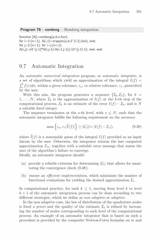
9.7 Automatic Integration 391
Program 76 - romberg : Romberg integration
function [A]=romberg(a,b,n,fun);for i=1:(n+1), A(i,1)=trapezc(a,b,2ˆ(i-1),fun); end;for j=2:(n+1), for i=j:(n+1),A(i,j)=(4ˆ(j-1)*A(i,j-1)-A(i-1,j-1))/(4ˆ(j-1)-1); end; end;
9.7 Automatic Integration
An automatic numerical integration program, or automatic integrator, isa set of algorithms which yield an approximation of the integral I(f) =@ ba f(x)dx, within a given tolerance, +a, or relative tolerance, +r, prescribed
by the user.With this aim, the program generates a sequence {Ik, Ek}, for k =
1, . . . , N , where Ik is the approximation of I(f) at the k-th step of thecomputational process, Ek is an estimate of the error I(f) " Ik, and is Na suitable fixed integer.
The sequence terminates at the s-th level, with s & N , such that theautomatic integrator fulfills the following requirement on the accuracy
maxR+a, +r|DI(f)|
S) |Es|(1 |I(f)" Is|), (9.38)
where DI(f) is a reasonable guess of the integral I(f) provided as an inputdatum by the user. Otherwise, the integrator returns the last computedapproximation IN , together with a suitable error message that warns theuser of the algorithm’s failure to converge.Ideally, an automatic integrator should:
(a) provide a reliable criterion for determining |Es| that allows for moni-toring the convergence check (9.38);
(b) ensure an e"cient implementation, which minimizes the number offunctional evaluations for yielding the desired approximation Is.
In computational practice, for each k ) 1, moving from level k to levelk + 1 of the automatic integration process can be done according to twodi!erent strategies, which we define as non adaptive or adaptive.
In the non adaptive case, the law of distribution of the quadrature nodesis fixed a priori and the quality of the estimate Ik is refined by increas-ing the number of nodes corresponding to each level of the computationalprocess. An example of an automatic integrator that is based on such aprocedure is provided by the composite Newton-Cotes formulae on m and

392 9. Numerical Integration
2m subintervals, respectively, at levels k and k+ 1, as described in Section9.7.1.
In the adaptive case, the positions of the nodes is not set a priori, but ateach level k of the process they depend on the information that has beenstored during the previous k" 1 levels. An adaptive automatic integrationalgorithm is performed by partitioning the interval [a, b] into successivesubdivisions which are characterized by a nonuniform density of the nodes,this density being typically higher in a neighborhood of strong gradientsor singularities of f . An example of an adaptive integrator based on theCavalieri-Simpson formula is described in Section 9.7.2.
9.7.1 Non Adaptive Integration AlgorithmsIn this section, we employ the composite Newton-Cotes formulae. Our aimis to devise a criterion for estimating the absolute error |I(f) " Ik| byusing Richardson extrapolation. From (9.26) and (9.27) it turns out that,for m ) 1 and n ) 0, In,m(f) has order of infinitesimal equal to Hn+p,with p = 2 for n even and p = 1 for n odd, where m, n and H = (b" a)/mare the number of partitions of [a, b], the number of quadrature nodes overeach subinterval and the constant length of each subinterval, respectively.By doubling the value of m (i.e., halving the stepsize H) and proceedingby extrapolation, we get
I(f)" In,2m(f) 1 12n+p
[I(f)" In,m(f)] . (9.39)
The use of the symbol 1 instead of = is due to the fact that the point *or -, where the derivative in (9.26) and (9.27) must be evaluated, changeswhen passing from m to 2m subintervals. Solving (9.39) with respect toI(f) yields the following absolute error estimate for In,2m(f)
I(f)" In,2m(f) 1 In,2m(f)" In,m(f)2n+p " 1
. (9.40)
If the composite Simpson rule is considered (i.e., n = 2), (9.40) predicts areduction of the absolute error by a factor of 15 when passing from m to 2msubintervals. Notice also that only 2m"1 extra functional evaluations areneeded to compute the new approximation I1,2m(f) starting from I1,m(f).Relation (9.40) is an instance of an a posteriori error estimate (see Chapter2, Section 2.3). It is based on the combined use of an a priori estimate (inthis case, (9.26) or (9.27)) and of two evaluations of the quantity to be ap-proximated (the integral I(f)) for two di!erent values of the discretizationparameter (that is, H = (b" a)/m).

9.7 Automatic Integration 393
Example 9.8 Let us employ the a posteriori estimate (9.40) in the case of thecomposite Simpson formula (n = p = 2), for the approximation of the integral
)^
0
(ex/2 + cos 4x)dx = 2(e) % 1) 0 7.621,
where we require the absolute error to be less than 10%4. For k = 0, 1, . . . , sethk = (b%a)/2k and denote by I2,m(k)(f) the integral of f which is computed usingthe composite Simpson formula on a grid of size hk with m(k) = 2k intervals. Wecan thus assume as a conservative estimate of the quadrature error the followingquantity
|Ek| = |I(f)% I2,m(k)(f)| 0 110
|I2,2m(k)(f)% I2,m(k)(f)| = |Ek|, k ! 1.
(9.41)
Table 9.11 shows the sequence of the estimated errors |Ek| and of the correspond-ing absolute errors |Ek| that have been actually made by the numerical integrationprocess. Notice that, when convergence has been achieved, the error estimatedby (9.41) is definitely higher than the actual error, due to the conservative choiceabove. •
k |Ek| |Ek| k |Ek| |Ek|0 3.156 2 0.10 4.52 · 10"5
1 0.42 1.047 3 5.8 · 10"6 2 · 10"9
TABLE 9.11. Non adaptive automatic Simpson rule for the approximation of@ )
0 (ex/2 + cos 4x)dx
An alternative approach for fulfilling the constraints (a) and (b) con-sists of employing a nested sequence of special Gaussian quadratures Ik(f)(see Chapter 10), having increasing degree of exactness for k = 1, . . . , N .These formulae are constructed in such a way that, denoting by Snk ={x1, . . . , xnk} the set of quadrature nodes relative to quadrature Ik(f),Snk * Snk+1 for any k = 1, . . . , N " 1. As a result, for k ) 1, the formulaat the k + 1-th level employs all the nodes of the formula at level k andthis makes nested formulae quite e!ective for computer implementation.
As an example, we recall the Gauss-Kronrod formulae with 10, 21, 43and 87 points, that are available in [PdKUK83] (in this case, N = 4). TheGauss-Kronrod formulae have degree of exactness rnk (optimal) equal to2nk"1, where nk is the number of nodes for each formula, with n1 = 10 andnk+1 = 2nk+1 for k = 1, 2, 3. The criterion for devising an error estimate isbased on comparing the results given by two successive formulae Ink(f) andInk+1(f) with k = 1, 2, 3, and then terminating the computational processat the level k such that (see also [DR75], p. 321)
|Ik+1 " Ik| & max {+a, +r|Ik+1|} .

394 9. Numerical Integration
9.7.2 Adaptive Integration AlgorithmsThe goal of an adaptive integrator is to yield an approximation of I(f)within a fixed tolerance + by a non uniform distribution of the integrationstepsize along the interval [a, b]. An optimal algorithm is able to adaptautomatically the choice of the steplength according to the behavior of theintegrand function, by increasing the density of the quadrature nodes wherethe function exhibits stronger variations.
In view of describing the method, it is convenient to restrict our attentionto a generic subinterval [",#] 7 [a, b]. Recalling the error estimates for theNewton-Cotes formulae, it turns out that the evaluation of the derivativesof f , up to a certain order, is needed to set a stepsize h such that a fixedaccuracy is ensured, say +(#"")/(b"a). This procedure, which is unfeasiblein practical computations, is carried out by an automatic integrator asfollows. We consider throughout this section the Cavalieri-Simpson formula(9.15), although the method can be extended to other quadrature rules.
Set If (",#) =@ '! f(x)dx, h = h0 = (# " ")/2 and
Sf (",#) = (h0/3) [f(") + 4f("+ h0) + f(#)] .
From (9.16) we get
If (",#)" Sf (",#) = "h50
90f (4)(*), (9.42)
where * is a point in (",#). To estimate the error If (",#) " Sf (",#)without using explicitly the function f (4) we employ again the Cavalieri-Simpson formula over the union of the two subintervals [", ("+ #)/2] and[("+ #)/2,#], obtaining, for h = h0/2 = (# " ")/4
If (",#)" Sf,2(",#) = " (h0/2)5
90
Kf (4)(*) + f (4)(-)
L,
where * ! (", (" + #)/2), - ! ((" + #)/2,#) and Sf,2(",#) = Sf (", (" +#)/2) + Sf (("+ #)/2,#).
Let us now make the assumption that f (4)(*) 1 f (4)(-) (which is true,in general, only if the function f (4) does not vary “too much” on [",#]).Then,
If (",#)" Sf,2(",#) 1 " 116
h50
90f (4)(*), (9.43)
with a reduction of the error by a factor 16 with respect to (9.42), corre-sponding to the choice of a steplength of doubled size. Comparing (9.42)and (9.43), we get the estimate
h50
90f (4)(*) 1 16
15Ef (",#),

9.7 Automatic Integration 395
where Ef (",#) = Sf (",#)" Sf,2(",#). Then, from (9.43), we have
|If (",#)" Sf,2(",#)| 1 |Ef (",#)|15
. (9.44)
We have thus obtained a formula that allows for easily computing the errormade by using composite Cavalieri-Simpson numerical integration on thegeneric interval [",#]. Relation (9.44), as well as (9.40), is another instanceof an a posteriori error estimate. It combines the use of an a priori es-timate (in this case, (9.16)) and of two evaluations of the quantity to beapproximated (the integral I(f)) for two di!erent values of the discretiza-tion parameter h.
In the practice, it might be convenient to assume a more conservativeerror estimate, precisely
|If (",#)" Sf,2(",#)| 1 |Ef (",#)|/10.
Moreover, to ensure a global accuracy on [a, b] equal to the fixed tolerance+, it will su"ce to enforce that the error Ef (",#) satisfies on each singlesubinterval [",#] 7 [a, b] the following constraint
|Ef (",#)|10
& +# " "b" a
. (9.45)
The adaptive automatic integration algorithm can be described as follows.Denote by:
1. A: the active integration interval, i.e., the interval where the integralis being computed;
2. S: the integration interval already examined, for which the error test(9.45) has been successfully passed;
3. N : the integration interval yet to be examined.
At the beginning of the integration process we have N = [a, b], A = Nand S = 9, while the situation at the generic step of the algorithm isdepicted in Figure 9.3. Set JS(f) 1
@ !a f(x)dx, with JS(f) = 0 at the
beginning of the process; if the algorithm successfully terminates, JS(f)yields the desired approximation of I(f). We also denote by J(!,')(f) theapproximate integral of f over the “active” interval [",#]. This intervalis drawn in bold in Figure 9.3. At each step of the adaptive integrationmethod the following decisions are taken:
1. if the local error test (9.45) is passed, then:
(i) JS(f) is increased by J(!,')(f), that is, JS(f) ; JS(f)+J(!,')(f);(ii) we let S ; S 2 A, A = N (corresponding to the path (I) in
Figure 9.3), # = b.

396 9. Numerical Integration
a
"*
b
b
b
" #S A N
(I)Sa
a
" A
"S A N
(II)
FIGURE 9.3. Distribution of the integration intervals at the generic step of theadaptive algorithm and updating of the integration grid
2. If the local error test (9.45) fails, then:
(j) A is halved, and the new active interval is set to A = [","*] with"* = ("+ #)/2 (corresponding to the path (II) in Figure 9.3);
(jj) we let N ; N 2 ["*,#], # ; "*;(jjj) a new error estimate is provided.
In order to prevent the algorithm from generating too small stepsizes, itis convenient to monitor the width of A and warn the user, in case ofan excessive reduction of the steplength, about the presence of a possiblesingularity in the integrand function (see Section 9.8).
Example 9.9 Let us employ Cavalieri-Simpson adaptive integration for com-puting the integral
I(f) =4^
%3
tan%1(10x)dx
= 4tan%1(40) + 3tan%1(%30)% (1/20) log(16/9) 0 1.54201193.
Running Program 77 with tol = 10%4 and hmin = 10%3 yields an approximationof the integral with an absolute error of 2.104 · 10%5. The algorithm performs77 functional evaluations, corresponding to partitioning the interval [a, b] into38 nonuniform subintervals. We notice that the corresponding composite formulawith uniform stepsize would have required 128 subintervals with an absolute errorof 2.413 · 10%5.
In Figure 9.4 (left) we show, together with the plot of the integrand function,the distribution of the quadrature nodes as a function of x, while on the rightthe integration step density (piecewise constant) $h(x) is shown, defined as theinverse of the step size h over each active interval A. Notice the high value attainedby $h at x = 0, where the derivative of the integrand function is maximum. •
The adaptive algorithm described above is implemented in Program 77.Among the input parameters, hmin is the minimum admissible value ofthe integration steplength. In output the program returns the approximate

9.7 Automatic Integration 397
!3 !2 !1 0 1 2 3 4!2
!1.5
!1
!0.5
0
0.5
1
1.5
2
!3 !2 !1 0 1 2 3 40
10
20
30
40
50
60
70
80
FIGURE 9.4. Distribution of quadrature nodes (left); density of the integrationstepsize in the approximation of the integral of Example 9.9 (right)
value of the integral integ, the total number of functional evaluations nfvand the set of integration points xfv.
Program 77 - simpadpt : Adaptive Cavalieri-Simpson formula
function [integ,xfv,nfv]=simpadpt(a,b,tol,fun,hmin);integ=0; level=0; i=1; alfa(i)=a; beta(i)=b;step=(beta(i)-alfa(i))/4; nfv=0;for k=1:5, x=a+(k-1)*step; f(i,k)=eval(fun); nfv=nfv+1; endwhile (i > 0),S=0; S2=0; h=(beta(i)-alfa(i))/2; S=(h/3)*(f(i,1)+4*f(i,3)+f(i,5));h=h/2; S2=(h/3)*(f(i,1)+4*f(i,2)+f(i,3));S2=S2+(h/3)*(f(i,3)+4*f(i,4)+f(i,5));tolrv=tol*(beta(i)-alfa(i))/(b-a); errrv=abs(S-S2)/10;if (errrv > tolrv)i=i+1; alfa(i)=alfa(i-1); beta(i)=(alfa(i-1)+beta(i-1))/2;f(i,1)=f(i-1,1);f(i,3)=f(i-1,2);f(i,5)=f(i-1,3);len=abs(beta(i)-alfa(i));if (len >= hmin),if (len <= 11*hmin)disp(’ Steplength close to hmin ’),str=sprintf(’The approximate integral is %12.7e’,integ);disp(str),end;step=len/4; x=alfa(i)+step; f(i,2)=eval(fun);nfv=nfv+1; x=beta(i)-step; f(i,4)=eval(fun); nfv=nfv+1;else, xfv=xfv’; disp(’ Too small steplength ’)str=sprintf(’The approximate integral is %12.7e’,integ);disp(str), return
end, elseinteg=integ+S2; level=level+1; if (level==1),for k=1:5, xfv(k)=alfa(i)+(k-1)*h; end; ist=5;else, for k=1:4, xfv(ist+k)=alfa(i)+k*h; end; ist=ist+4; end;if (beta(i)==b), xfv=xfv’;str=sprintf(’The approximate integral is %12.7e’,integ);disp(str), return, end; i=i-1; alfa(i)=beta(i+1);f(i,1)=f(i+1,5); f(i,3)=f(i,4); step=abs(beta(i)-alfa(i))/4;x=alfa(i)+step; f(i,2)=eval(fun); nfv=nfv+1; x=beta(i)-step;f(i,4)=eval(fun); nfv=nfv+1;

398 9. Numerical Integration
endend
9.8 Singular Integrals
In this section we extend our analysis to deal with singular integrals, arisingwhen f has finite jumps or is even infinite at some point. Besides, wewill consider the case of integrals of bounded functions over unboundedintervals. We briefly address the most relevant numerical techniques forproperly handling these integrals.
9.8.1 Integrals of Functions with Finite Jump DiscontinuitiesLet c be a known point within [a, b] and assume that f is a continuous andbounded function in [a, c) and (c, b], with finite jump f(c+)" f(c"). Since
I(f) =^ b
af(x)dx =
^ c
af(x)dx +
^ b
cf(x)dx, (9.46)
any integration formula of the previous sections can be used on [a, c"] and[c+, b] to furnish an approximation of I(f). We proceed similarly if f admitsa finite number of jump discontinuities within [a, b].
When the position of the discontinuity points of f is not known a priori,a preliminary analysis of the graph of the function should be carried out.Alternatively, one can resort to an adaptive integrator that is able to detectthe presence of discontinuities when the integration steplength falls belowa given tolerance (see Section 9.7.2).
9.8.2 Integrals of Infinite FunctionsLet us deal with the case in which limx&a+ f(x) = ,; similar consider-ations hold when f is infinite as x ( b", while the case of a point ofsingularity c internal to the interval [a, b] can be recast to one of the pre-vious two cases owing to (9.46). Assume that the integrand function is ofthe form
f(x) =4(x)
(x" a)µ, 0 & µ < 1,
where 4 is a function whose absolute value is bounded by M . Then
|I(f)| &M limt&a+
b^
t
1(x" a)µ
dx = M(b" a)1"µ
1" µ.

9.8 Singular Integrals 399
Suppose we wish to approximate I(f) up to a fixed tolerance %. For this, letus describe the following two methods (for further details, see also [IK66],Section 7.6, and [DR75], Section 2.12 and Appendix 1).
Method 1. For any + such that 0 < + < (b " a), we write the singularintegral as I(f) = I1 + I2, where
I1 =a+%^
a
4(x)(x" a)µ
dx, I2 =b^
a+%
4(x)(x" a)µ
dx.
The computation of I2 is not troublesome. After replacing 4 by its p-thorder Taylor’s expansion around x = a, we obtain
4(x) = 'p(x) +(x" a)p+1
(p + 1)!4(p+1)(*(x)), p ) 0 (9.47)
where 'p(x) =!p
k=0 4(k)(a)(x" a)k/k!. Then
I1 = +1"µp(
k=0
+k4(k)(a)k!(k + 1" µ)
+1
(p + 1)!
a+%^
a
(x" a)p+1"µ4(p+1)(*(x))dx.
Replacing I1 by the finite sum, the corresponding error E1 can be boundedas
|E1| &+p+2"µ
(p + 1)!(p + 2" µ)max
a%x%a+%|4(p+1)(x)|, p ) 0. (9.48)
For fixed p, the right side of (9.48) is an increasing function of +. On theother hand, taking + < 1 and assuming that the successive derivatives of 4do not grow too much as p increases, the same function is decreasing as pgrows.
Let us next approximate I2 using a composite Newton-Cotes formulawith m subintervals and n quadrature nodes for each subinterval, n beingan even integer. Recalling (9.26) and aiming at equidistributing the error% between I1 and I2, it turns out that
|E2| &M(n+2)(+)b" a" +(n + 2)!
|Mn|nn+3
4b" a" +
m
5n+2
= %/2, (9.49)
whereM(n+2)(+) = max
a+%%x%b
>>>>dn+2
dxn+2
44(x)
(x" a)µ
5>>>> .
The value of the constant M(n+2)(+) grows rapidly as + tends to zero; asa consequence, (9.49) might require such a large number of subintervalsm% = m(+) to make the method at hand of little practical use.
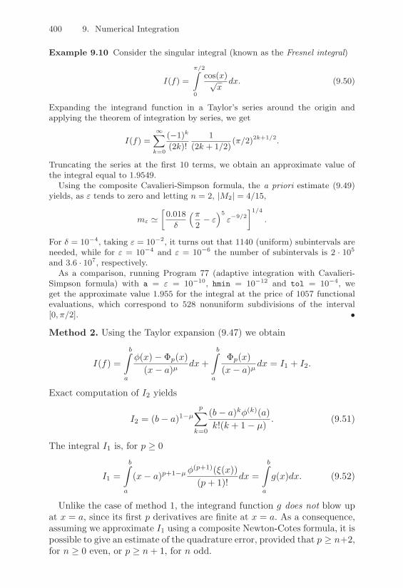
400 9. Numerical Integration
Example 9.10 Consider the singular integral (known as the Fresnel integral)
I(f) =
)/2^
0
cos(x)'x
dx. (9.50)
Expanding the integrand function in a Taylor’s series around the origin andapplying the theorem of integration by series, we get
I(f) =!(
k=0
(%1)k
(2k)!1
(2k + 1/2)(+/2)2k+1/2.
Truncating the series at the first 10 terms, we obtain an approximate value ofthe integral equal to 1.9549.
Using the composite Cavalieri-Simpson formula, the a priori estimate (9.49)yields, as & tends to zero and letting n = 2, |M2| = 4/15,
m' 0-0.018
!
K+2% &
L5&%9/2
.1/4
.
For ! = 10%4, taking & = 10%2, it turns out that 1140 (uniform) subintervals areneeded, while for & = 10%4 and & = 10%6 the number of subintervals is 2 · 105
and 3.6 · 107, respectively.As a comparison, running Program 77 (adaptive integration with Cavalieri-
Simpson formula) with a = & = 10%10, hmin = 10%12 and tol = 10%4, weget the approximate value 1.955 for the integral at the price of 1057 functionalevaluations, which correspond to 528 nonuniform subdivisions of the interval[0,+/2]. •
Method 2. Using the Taylor expansion (9.47) we obtain
I(f) =b^
a
4(x)" 'p(x)(x" a)µ
dx +b^
a
'p(x)(x" a)µ
dx = I1 + I2.
Exact computation of I2 yields
I2 = (b" a)1"µp(
k=0
(b" a)k4(k)(a)k!(k + 1" µ)
. (9.51)
The integral I1 is, for p ) 0
I1 =b^
a
(x" a)p+1"µ4(p+1)(*(x))(p + 1)!
dx =b^
a
g(x)dx. (9.52)
Unlike the case of method 1, the integrand function g does not blow upat x = a, since its first p derivatives are finite at x = a. As a consequence,assuming we approximate I1 using a composite Newton-Cotes formula, it ispossible to give an estimate of the quadrature error, provided that p ) n+2,for n ) 0 even, or p ) n + 1, for n odd.

9.8 Singular Integrals 401
Example 9.11 Consider again the singular Fresnel integral (9.50), and assumewe use the composite Cavalieri-Simpson formula for approximating I1. We willtake p = 4 in (9.51) and (9.52). Computing I2 yields the value (+/2)1/2(2 %(1/5)(+/2)2 + (1/108)(+/2)4) 0 1.9588. Applying the error estimate (9.26) withn = 2 shows that only 2 subdivisions of [0,+/2] su!ce for approximating I1 upto an error ! = 10%4, obtaining the value I1 0 %0.0173. As a whole, method 2returns for (9.50) the approximate value 1.9415. •
9.8.3 Integrals over Unbounded IntervalsLet f ! C0([a,+,)); should it exist and be finite, the following limit
limt&+$
t^
a
f(x)dx
is taken as being the value of the singular integral
I(f) =^ $
af(x)dx = lim
t&+$
t^
a
f(x)dx. (9.53)
An analogous definition holds if f is continuous over (",, b], while for afunction f : R ( R, integrable over any bounded interval, we let
^ $
"$f(x)dx =
^ c
"$f(x)dx +
^ +$
cf(x)dx (9.54)
if c is any real number and the two singular integrals on the right hand sideof (9.54) are convergent. This definition is correct since the value of I(f)does not depend on the choice of c.A su"cient condition for f to be integrable over [a,+,) is that
-) > 0, such that limx&+$
x1++f(x) = 0,
that is, we require f to be infinitesimal of order > 1 with respect to 1/xas x(,. For the numerical approximation of (9.53) up to a tolerance %,we consider the following methods, referring for further details to [DR75],Chapter 3.
Method 1. To compute (9.53), we can split I(f) as I(f) = I1 + I2, whereI1 =
@ ca f(x)dx and I2 =
@ $c f(x)dx.
The end-point c, which can be taken arbitrarily, is chosen in such a waythat the contribution of I2 is negligible. Precisely, taking advantage of theasymptotic behavior of f , c is selected to guarantee that I2 equals a fractionof the fixed tolerance, say, I2 = %/2.
Then, I1 will be computed up to an absolute error equal to %/2. Thisensures that the global error in the computation of I1 + I2 is below thetolerance %.

402 9. Numerical Integration
Example 9.12 Compute up to an error ! = 10%3 the integral
I(f) =!
0
cos2(x)e%xdx = 3/5.
For any given c > 0, we have I2 =!
c
cos2(x)e%xdx "^ !
c
e%xdx = e%c; re-
quiring that e%c = !/2, one gets c 0 7.6. Then, assuming we use the compos-ite trapezoidal formula for approximating I1, thanks to (9.27) with n = 1 andM = max0*x*c |f (((x)| 0 1.04, we obtain m !
8Mc3/(6!)
91/2 = 277.Program 72 returns the value I1 0 0.599905, instead of the exact value I1 =
3/5% e%c(cos2(c)% (sin(2c) + 2 cos(2c))/5) 0 0.599842, with an absolute error ofabout 6.27 · 10%5. The global numerical outcome is thus I1 + I2 0 0.600405, withan absolute error with respect to I(f) equal to 4.05 · 10%4. •
Method 2. For any real number c, we let I(f) = I1 + I2, as for method 1,then we introduce the change of variable x = 1/t in order to transform I2into an integral over the bounded interval [0, 1/c]
I2 =
1/c^
0
f(t)t"2dt =
1/c^
0
g(t)dt. (9.55)
If g(t) is not singular at t = 0, (9.55) can be treated by any quadratureformula introduced in this chapter. Otherwise, one can resort to the inte-gration methods considered in Section 9.8.2.
Method 3. Gaussian interpolatory formulae are used, where the integra-tion nodes are the zeros of Laguerre and Hermite orthogonal polynomials(see Section 10.5).
9.9 Multidimensional Numerical Integration
Let ( be a bounded domain in R2 with a su"ciently smooth boundary. Weconsider the problem of approximating the integral I(f) =
@" f(x, y)dxdy,
where f is a continuous function in (. For this purpose, in Sections 9.9.1and 9.9.2 we address two methods.
The first method applies when ( is a normal domain with respect to acoordinate axis. It is based on the reduction formula for double integralsand consists of using one-dimensional quadratures along both coordinatedirection. The second method, which applies when ( is a polygon, consistsof employing composite quadratures of low degree on a triangular decom-position of the domain (. Section 9.9.3 briefly addresses the Monte Carlo

9.9 Multidimensional Numerical Integration 403
method, which is particularly well-suited to integration in several dimen-sions.
9.9.1 The Method of Reduction FormulaLet ( be a normal domain with respect to the x axis, as drawn in Figure9.5, and assume for the sake of simplicity that 42(x) > 41(x), #x ! [a, b].
FIGURE 9.5. Normal domain with respect to x axis
The reduction formula for double integrals gives (with obvious choice ofnotation)
I(f) =b^
a
,2(x)^
,1(x)
f(x, y)dydx =b^
a
Ff (x)dx. (9.56)
The integral I(Ff ) =@ ba Ff (x)dx can be approximated by a composite
quadrature rule using Mx subintervals {Jk, k = 1, . . . ,Mx}, of width H =(b " a)/Mx, and in each subinterval n(k)
x + 1 nodes {xki , i = 0, . . . , n(k)
x }.Thus, in the x direction we can write
Icnx(f) =
Mx(
k=1
n(k)x(
i=0
"ki Ff (xk
i ),
where the coe"cients "ki are the quadrature weights on each subinterval Jk.
For each node xki , the approximate evaluation of the integral Ff (xk
i ) is thencarried out by a composite quadrature using My subintervals {Jm, m =1, . . . ,My}, of width hk
i = (42(xki ) " 41(xk
i ))/My and in each subintervaln(m)y + 1 nodes {yi,kj,m, j = 0, . . . , n(m)
y }.In the particular case Mx = My = M , n(k)
x = n(m)y = 0, for k,m =
1, . . . ,M , the resulting quadrature formula is the midpoint reduction for-mula
Ic0,0(f) = HM(
k=1
hk0
M(
m=1
f(xk0 , y
0,k0,m),

404 9. Numerical Integration
where H = (b " a)/M , xk0 = a + (k " 1/2)H for k = 1, . . . ,M and
y0,k0,m = 41(xk
0) + (m" 1/2)hk0 for m = 1, . . . ,M . With a similar procedure
the trapezoidal reduction formula can be constructed along the coordinatedirections (in that case, n(k)
x = n(m)y = 1, for k,m = 1, . . . ,M).
The e"ciency of the approach can obviously be increased by employingthe adaptive method described in Section 9.7.2 to suitably allocate thequadrature nodes xk
i and yi,kj,m according to the variations of f over thedomain (. The use of the reduction formulae above becomes less and lessconvenient as the dimension d of the domain ( * Rd gets larger, due tothe large increase in the computational e!ort. Indeed, if any simple integralrequires N functional evaluations, the overall cost would be equal to Nd.
The midpoint and trapezoidal reduction formulae for approximating theintegral (9.56) are implemented in Programs 78 and 79. For the sake ofsimplicity, we set Mx = My = M . The variables phi1 and phi2 containthe expressions of the functions 41 and 42 which delimitate the integrationdomain.
Program 78 - redmidpt : Midpoint reduction formula
function inte=redmidpt(a,b,phi1,phi2,m,fun)H=(b-a)/m; xx=[a+H/2:H:b]; dim=max(size(xx));for i=1:dim, x=xx(i); d=eval(phi2); c=eval(phi1); h=(d-c)/m;y=[c+h/2:h:d]; w=eval(fun); psi(i)=h*sum(w(1:m)); end;inte=H*sum(psi(1:m));
Program 79 - redtrap : Trapezoidal reduction formula
function inte=redtrap(a,b,phi1,phi2,m,fun)H=(b-a)/m; xx=[a:H:b]; dim=max(size(xx));for i=1:dim, x=xx(i); d=eval(phi2); c=eval(phi1); h=(d-c)/m;y=[c:h:d]; w=eval(fun); psi(i)=h*(0.5*w(1)+sum(w(2:m))+0.5*w(m+1));end; inte=H*(0.5*psi(1)+sum(psi(2:m))+0.5*psi(m+1));
9.9.2 Two-Dimensional Composite QuadraturesIn this section we extend to the two-dimensional case the composite inter-polatory quadratures that have been considered in Section 9.4. We assumethat ( is a convex polygon on which we introduce a triangulation Th of NT
triangles or elements, such that ( =M
T#Th
T , where the parameter h > 0 is
the maximum edge-length in Th (see Section 8.5.2).Exactly as happens in the one-dimensional case, interpolatory compositequadrature rules on triangles can be devised by replacing
@" f(x, y)dxdy
with@"$
khf(x, y)dxdy, where, for k ) 0, $k
hf is the composite interpolat-ing polynomial of f on the triangulation Th introduced in Section 8.5.2.

9.9 Multidimensional Numerical Integration 405
For an e"cient evaluation of this last integral, we employ the property ofadditivity which, combined with (8.38), leads to the following interpolatorycomposite rule
Ick(f) =^
"
$khf(x, y)dxdy =
(
T#Th
^
T
$kT f(x, y)dxdy =
(
T#Th
ITk (f)
=(
T#Th
dk"1(
j=0
f(zTj )^
T
lTj (x, y)dxdy =(
T#Th
dk"1(
j=0
"Tj f(zTj ).
(9.57)
The coe"cients "(j)T and the points z(j)
T are called the local weights andnodes of the quadrature formula (9.57), respectively.
The weights "(j)T can be computed on the reference triangle T of vertices
(0, 0), (1, 0) and (0, 1), as follows
"(j)T =
^
T
lj,T (x, y)dxdy = 2|T |^
T
lj(x, y)dxdy, j = 0, . . . , dk " 1,
where |T | is the area of T . If k = 0, we get "(0)T = |T |, while if k = 1 we
have "(j)T = |T |/3, for j = 0, 1, 2.
Denoting respectively by a(j)T and aT =
!3j=1(a
(j)T )/3, for j = 1, 2, 3, the
vertices and the center of gravity of the triangle T ! Th, the followingformulae are obtained.
Composite midpoint formula
Ic0(f) =(
T#Th
|T |f(aT ). (9.58)
Composite trapezoidal formula
Ic1(f) =13
(
T#Th
|T |3(
j=1
f(a(j)T ). (9.59)
In view of the analysis of the quadrature error Eck(f) = I(f) " Ick(f), we
introduce the following definition.
Definition 9.1 The quadrature formula (9.57) has degree of exactnessequal to n, with n ) 0, if I
:Tk (p) =
@:T pdxdy for any p ! Pn( :T ), where
Pn( :T ) is defined in (8.35). !
The following result can be proved (see [IK66], pp. 361–362).

406 9. Numerical Integration
Property 9.4 Assume that the quadrature rule (9.57) has degree of exact-ness on ( equal to n, with n ) 0, and that its weights are all nonnegative.Then, there exists a positive constant Kn, independent of h, such that
|Eck(f)| & Knh
n+1|(|Mn+1,
for any function f ! Cn+1((), where Mn+1 is the maximum value of themodules of the derivatives of order n + 1 of f and |(| is the area of (.
The composite formulae (9.58) and (9.59) both have degrees of exactnessequal to 1; then, due to Property 9.4, their order of infinitesimal withrespect to h is equal to 2.An alternative family of quadrature rules on triangles is provided by the so-called symmetric formulae. These are Gaussian formulae with n nodes andhigh degree of exactness, and exhibit the feature that the quadrature nodesoccupy symmetric positions with respect to all corners of the referencetriangle :T or, as happens for Gauss-Radau formulae, with respect to thestraight line :y = :x.Considering the generic triangle T ! Th and denoting by aT
(j), j = 1, 2, 3,the midpoints of the edges of T , two examples of symmetric formulae,having degree of exactness equal to 2 and 3, respectively, are the following
I3(f) =|T |3
3(
j=1
f(aT(j)), n = 3,
I7(f) =|T |60
G
H33(
i=1
f(a(i)T ) + 8
3(
j=1
f(aT(j)) + 27f(aT )
I
J , n = 7.
For a description and analysis of symmetric formulae for triangles, see[Dun85], while we refer to [Kea86] and [Dun86] for their extension to tetra-hedra and cubes.
The composite quadrature rules (9.58) and (9.59) are implemented inPrograms 80 and 81 for the approximate evaluation of the integral of f(x, y)over a single triangle T ! Th. To compute the integral over ( it su"cesto sum the result provided by the program over each triangle of Th. Thecoordinates of the vertices of the triangle T are stored in the arrays xv andyv.
Program 80 - midptr2d : Midpoint rule on a triangle
function inte=midptr2d(xv,yv,fun)y12=yv(1)-yv(2); y23=yv(2)-yv(3); y31=yv(3)-yv(1);areat=0.5*abs(xv(1)*y23+xv(2)*y31+xv(3)*y12);x=sum(xv)/3; y=sum(yv)/3; inte=areat*eval(fun);
Program 81 - traptr2d : Trapezoidal rule on a triangle

9.9 Multidimensional Numerical Integration 407
function inte=traptr2d(xv,yv,fun)y12=yv(1)-yv(2); y23=yv(2)-yv(3); y31=yv(3)-yv(1);areat=0.5*abs(xv(1)*y23+xv(2)*y31+xv(3)*y12); inte=0;for i=1:3, x=xv(i); y=yv(i); inte=inte+eval(fun); end;inte=inte*areat/3;
9.9.3 Monte Carlo Methods for Numerical IntegrationNumerical integration methods based on Monte Carlo techniques are a validtool for approximating multidimensional integrals when the space dimen-sion of Rn gets large. These methods di!er from the approaches consideredthus far, since the choice of quadrature nodes is done statistically accord-ing to the values attained by random variables having a known probabilitydistribution.
The basic idea of the method is to interpret the integral as a statisticmean value
^
"
f(x)dx = |(|^
Rn
|(|"17"(x)f(x)dx = |(|µ(f),
where x = (x1, x2, . . . , xn)T and |(| denotes the n-dimensional volume of(, 7"(x) is the characteristic function of the set (, equal to 1 for x ! ( andto 0 elsewhere, while µ(f) is the mean value of the function f(X), whereX is a random variable with uniform probability density |(|"17" over Rn.
We recall that the random variable X ! Rn (or, more properly, randomvector) is an n-tuple of real numbers X1(8), . . . , Xn(8) assigned to everyoutcome 8 of a random experiment (see [Pap87], Chapter 4).
Having fixed a vector x ! Rn, the probability P{X & x} of the randomevent {X1 & x1, . . . , Xn & xn} is given by
P{X & x} =^ x1
"$. . .
^ xn
"$f(X1, . . . , Xn)dX1 . . . dXn
where f(X) = f(X1, . . . , Xn) is the probability density of the random vari-able X ! Rn, such that
f(X1, . . . , Xn) ) 0,^
Rn
f(X1, . . . , Xn)dX = 1.
The numerical computation of the mean value µ(f) is carried out by takingN independent samples x1, . . . ,xN ! Rn with probability density |(|"17"and evaluating their average
fN =1N
N(
i=1
f(xi) = IN (f). (9.60)
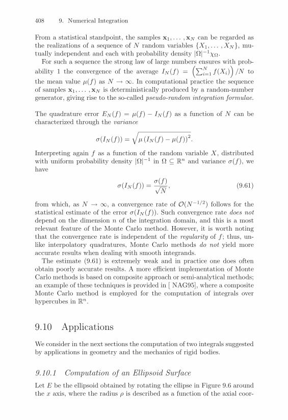
408 9. Numerical Integration
From a statistical standpoint, the samples x1, . . . ,xN can be regarded asthe realizations of a sequence of N random variables {X1, . . . , XN}, mu-tually independent and each with probability density |(|"17".
For such a sequence the strong law of large numbers ensures with prob-ability 1 the convergence of the average IN (f) =
K!Ni=1 f(Xi)
L/N to
the mean value µ(f) as N ( ,. In computational practice the sequenceof samples x1, . . . ,xN is deterministically produced by a random-numbergenerator, giving rise to the so-called pseudo-random integration formulae.
The quadrature error EN (f) = µ(f) " IN (f) as a function of N can becharacterized through the variance
((IN (f)) =2µ (IN (f)" µ(f))2.
Interpreting again f as a function of the random variable X, distributedwith uniform probability density |(|"1 in ( 7 Rn and variance ((f), wehave
((IN (f)) =((f)/N
, (9.61)
from which, as N ( ,, a convergence rate of O(N"1/2) follows for thestatistical estimate of the error ((IN (f)). Such convergence rate does notdepend on the dimension n of the integration domain, and this is a mostrelevant feature of the Monte Carlo method. However, it is worth notingthat the convergence rate is independent of the regularity of f ; thus, un-like interpolatory quadratures, Monte Carlo methods do not yield moreaccurate results when dealing with smooth integrands.
The estimate (9.61) is extremely weak and in practice one does oftenobtain poorly accurate results. A more e"cient implementation of MonteCarlo methods is based on composite approach or semi-analytical methods;an example of these techniques is provided in [ NAG95], where a compositeMonte Carlo method is employed for the computation of integrals overhypercubes in Rn.
9.10 Applications
We consider in the next sections the computation of two integrals suggestedby applications in geometry and the mechanics of rigid bodies.
9.10.1 Computation of an Ellipsoid SurfaceLet E be the ellipsoid obtained by rotating the ellipse in Figure 9.6 aroundthe x axis, where the radius ) is described as a function of the axial coor-

9.10 Applications 409
x )"
1/#- 1/#
(
x
E
FIGURE 9.6. Section of the ellipsoid
dinate by the equation
)2(x) = "2(1" #2x2), " 1#& x & 1
#,
" and # being given constants, assigned in such a way that "2#2 < 1.We set the following values for the parameters: "2 = (3 " 2
/2)/100 and
#2 = 100. Letting K2 = #23
1" "2#2, f(x) =/
1"K2x2 and ! =cos"1(K/#), the computation of the surface of E requires evaluating theintegral
I(f) = 4&"
1/'^
0
f(x)dx =2&"K
[(&/2" !) + sin(2!)/2] . (9.62)
Notice that f *(1/#) = "100; this prompts us to use a numerical adaptiveformula able to provide a nonuniform distribution of quadrature nodes,with a possible refinement of these nodes around x = 1/#.Table 9.12 summarizes the results obtained using the composite midpoint,trapezoidal and Cavalieri-Simpson rules (respectively denoted by (MP),(TR) and (CS)), which are compared with Romberg integration (RO) andwith the adaptive Cavalieri-Simpson quadrature introduced in Section 9.7.2and denoted by (AD).
In the table, m is the number of subintervals, while Err and flops denotethe absolute quadrature error and the number of floating-point operationsrequired by each algorithm, respectively. In the case of the AD method,we have run Program 77 taking hmin=10"5 and tol=10"8, while for theRomberg method we have used Program 76 with n=9.The results demonstrate the advantage of using the composite adaptiveCavalieri-Simpson formula, both in terms of computational e"ciency andaccuracy, as can be seen in the plots in Figure 9.7 which allow to checkthe successful working of the adaptivity procedure. In Figure 9.7 (left),we show, together with the graph of f , the nonuniform distribution ofthe quadrature nodes on the x axis, while in Figure 9.7 (right) we plotthe logarithmic graph of the integration step density (piecewise constant)#h(x), defined as the inverse of the value of the stepsize h on each activeinterval A (see Section 9.7.2).

410 9. Numerical Integration
Notice the high value of #h at x = 1/#, where the derivative of theintegrand function is maximum.
(PM) (TR) (CS) (RO) (AD)m 4000 5600 250 50Err 3.24e" 10 3.30e" 10 2.98e" 10 3.58e" 11 3.18e" 10flops 20007 29013 2519 5772 3540
TABLE 9.12. Methods for approximating I(f) = 4+$@ 1/"
0
'1%K2x2dx, with
$2 = (3% 2'
2)/100, ) = 10 and K2 =3
)2(1% $2)2)
0 0.02 0.04 0.06 0.08 0.1!0.2
0
0.2
0.4
0.6
0.8
1
0 0.02 0.04 0.06 0.08 0.110
2
103
104
105
FIGURE 9.7. Distribution of quadrature nodes (left); integration stepsize densityin the approximation of integral (9.62) (right)
9.10.2 Computation of the Wind Action on a Sailboat MastLet us consider the sailboat schematically drawn in Figure 9.8 (left) andsubject to the action of the wind force. The mast, of length L, is denoted bythe straight line AB, while one of the two shrouds (strings for the side sti!-ening of the mast) is represented by the straight line BO. Any infinitesimalelement of the sail transmits to the corresponding element of length dx ofthe mast a force of magnitude equal to f(x)dx. The change of f along withthe height x, measured from the point A (basis of the mast), is expressedby the following law
f(x) ="x
x + #e"-x,
where ", # and ' are given constants.

9.10 Applications 411
The resultant R of the force f is defined as
R =L
0
f(x)dx ? I(f), (9.63)
and is applied at a point at distance equal to b (to be determined) fromthe basis of the mast.
dx
winddirection
mast
shroud
TA
O
dx
B
fL
AO
V
B
T
M
H
b
R
FIGURE 9.8. Schematic representation of a sailboat (left); forces acting on themast (right)
Computing R and the distance b, given by b = I(xf)/I(f), is crucial for thestructural design of the mast and shroud sections. Indeed, once the valuesof R and b are known, it is possible to analyze the hyperstatic structuremast-shroud (using for instance the method of forces), thus allowing for thecomputation of the reactions V , H and M at the basis of the mast and thetraction T that is transmitted by the shroud, and are drawn in Figure 9.8(right). Then, the internal actions in the structure can be found, as well asthe maximum stresses arising in the mast AB and in the shroud BO, fromwhich, assuming that the safety verifications are satisfied, one can finallydesign the geometrical parameters of the sections of AB and BO.For the approximate computation of R we have considered the compos-ite midpoint, trapezoidal and Cavalieri-Simpson rules, denoted henceforthby (MP), (TR) and (CS), and, for a comparison, the adaptive Cavalieri-Simpson quadrature formula introduced in Section 9.7.2 and denoted by(AD). Since a closed-form expression for the integral (9.63) is not available,the composite rules have been applied taking mk = 2k uniform partitionsof [0, L], with k = 0, . . . , 15.
We have assumed in the numerical experiments " = 50, # = 5/3 and' = 1/4 and we have run Program 77 taking tol=10"4 and hmin=10"3.The sequence of integrals computed using the composite formulae has beenstopped at k = 12 (corresponding to mk = 212 = 4096) since the remaining

412 9. Numerical Integration
0 20 40 60 80 100 12010
!9
10!8
10!7
10!6
10!5
10!4
10!3
10!2
10!1
100
(TR)
(PM)
(CS)
(AD)
FIGURE 9.9. Relative errors in the approximate computation of the integral@ L
0 ($xe%*x)/(x + ))dx
elements, in the case of formula CS, di!er among them only up to the lastsignificant figure. Therefore, we have assumed as the exact value of I(f)the outcome I(CS)
12 = 100.0613683179612 provided by formula CS.We report in Figure 9.9 the logarithmic plots of the relative error |I(CS)
12 "Ik|/I12, for k = 0, . . . , 7, Ik being the generic element of the sequence forthe three considered formulae. As a comparison, we also display the graphof the relative error in the case of formula AD, applied on a number of(nonuniform) partitions equivalent to that of the composite rules.Notice how, for the same number of partitions, formula AD is more accu-rate, with a relative error of 2.06 · 10"7 obtained using 37 (nonuniform)partitions of [0, L]. Methods PM and TR achieve a comparable accuracyemploying 2048 and 4096 uniform subintervals, respectively, while formulaCS requires about 64 partitions. The e!ectiveness of the adaptivity pro-cedure is demonstrated by the plots in Figure 9.10, which show, togetherwith the graph of f , the distribution of the quadrature nodes (left) and thefunction #h(x) (right) that expresses the (piecewise constant) density ofthe integration stepsize h, defined as the inverse of the value of h over eachactive interval A (see Section 9.7.2).
Notice also the high value of #h at x = 0, where the derivatives of f aremaximum.
9.11 Exercises1. Let E0(f) and E1(f) be the quadrature errors in (9.6) and (9.12). Prove
that |E1(f)| 0 2|E0(f)|.
2. Check that the error estimates for the midpoint, trapezoidal and Cavalieri-Simpson formulae, given respectively by (9.6), (9.12) and (9.16), are specialinstances of (9.19) or (9.20). In particular, show that M0 = 2/3, K1 =

9.11 Exercises 413
0 2 4 6 8 10!5
0
5
10
15
20
0 2 4 6 8 100
5
10
15
20
25
30
FIGURE 9.10. Distribution of quadrature nodes (left); integration step densityin the approximation of the integral
@ L
0 ($xe%*x)/(x + ))dx (right)
%1/6 and M2 = %4/15 and determine, using the definition, the degree ofexactness r of each formula.[Hint: find r such that In(xk) =
@ b
axkdx, for k = 0, . . . , r, and In(xj) $=@ b
axjdx, for j > r.]
3. Let In(f) =!n
k=0 $kf(xk) be a Lagrange quadrature formula on n + 1nodes. Compute the degree of exactness r of the formulae:
(a) I2(f) = (2/3)[2f(%1/2)% f(0) + 2f(1/2)],
(b) I4(f) = (1/4)[f(%1) + 3f(%1/3) + 3f(1/3) + f(1)].
Which is the order of infinitesimal p for (a) and (b)?[Solution: r = 3 and p = 5 for both I2(f) and I4(f).]
4. Compute df [x0, . . . , xn, x]/dx by checking (9.22).[Hint: proceed by computing directly the derivative at x as an incrementalratio, in the case where only one node x0 exists, then upgrade progressivelythe order of the divided di"erence.]
5. Let Iw(f) =@ 10 w(x)f(x)dx with w(x) =
'x, and consider the quadrature
formula Q(f) = af(x1). Find a and x1 in such a way that Q has maximumdegree of exactness r.[Solution: a = 2/3, x1 = 3/5 and r = 1.]
6. Let us consider the quadrature formula Q(f) = $1f(0) +$2f(1) +$3f((0)
for the approximation of I(f) =@ 10 f(x)dx, where f / C1([0, 1]). Determine
the coe!cients $j , for j = 1, 2, 3 in such a way that Q has degree ofexactness r = 2.[Solution: $1 = 2/3, $2 = 1/3 and $3 = 1/6.]
7. Apply the midpoint, trapezoidal and Cavalieri-Simpson composite rules toapproximate the integral ^ 1
%1|x|exdx,
and discuss their convergence as a function of the size H of the subintervals.

414 9. Numerical Integration
8. Consider the integral I(f) =@ 10 exdx and estimate the minimum number m
of subintervals that is needed for computing I(f) up to an absolute error" 5 · 10%4 using the composite trapezoidal (TR) and Cavalieri-Simpson(CS) rules. Evaluate in both cases the absolute error Err that is actuallymade.[Solution: for TR, we have m = 17 and Err = 4.95 · 10%4, while for CS,m = 2 and Err = 3.70 · 10%5.]
9. Consider the corrected trapezoidal formula (9.30) and check that |Ecorr1 (f)| 0
4|E2(f)|, where Ecorr1 (f) and E2(f) are defined in (9.31) and (9.16), re-
spectively.
10. Compute, with an error less than 10%4, the following integrals:
(a)@ !0 sin(x)/(1 + x4)dx;
(b)@ !0 e%x(1 + x)%5dx;
(c)@ !%! cos(x)e%x2
dx.
11. Use the reduction midpoint and trapezoidal formulae for computing thedouble integral I(f) =
@!
y(1 + xy)
dxdy over the domain ) = (0, 1)2. Run
Programs 78 and 79 with M = 2i, for i = 0, . . . , 10 and plot in log-scalethe absolute error in the two cases as a function of M . Which method isthe most accurate? How many functional evaluations are needed to get an(absolute) accuracy of the order of 10%6?[Solution: the exact integral is I(f) = log(4)% 1, and almost 2002 = 40000functional evaluations are needed.]

10Orthogonal Polynomials inApproximation Theory
Trigonometric polynomials, as well as other orthogonal polynomials likeLegendre’s and Chebyshev’s, are widely employed in approximation theory.
This chapter addresses the most relevant properties of orthogonal poly-nomials, and introduces the transforms associated with them, in particularthe discrete Fourier transform and the FFT, but also the Zeta and Wavelettransforms.
Application to interpolation, least-squares approximation, numerical dif-ferentiation and Gaussian integration are addressed.
10.1 Approximation of Functions by GeneralizedFourier Series
Let w = w(x) be a weight function on the interval ("1, 1), i.e., a nonneg-ative integrable function in ("1, 1). Let us denote by {pk, k = 0, 1, . . . } asystem of algebraic polynomials, with pk of degree equal to k for each k,mutually orthogonal on the interval ("1, 1) with respect to w. This meansthat
1^
"1
pk(x)pm(x)w(x)dx = 0 if k '= m.
416 10. Orthogonal Polynomials in Approximation Theory
Set (f, g)w =@ 1"1 f(x)g(x)w(x)dx and +f+w = (f, f)1/2w ; (·, ·)w and + · +w
are respectively the scalar product and the norm for the function space
L2w = L2
w("1, 1) =Ef : ("1, 1) ( R,
^ 1
"1f2(x)w(x)dx <,
F. (10.1)
For any function f ! L2w the series
Sf =+$(
k=0
:fkpk, with :fk =(f, pk)w+pk+2w
,
is called the generalized Fourier series of f , and :fk is the k-th Fouriercoe"cient. As is well-known, Sf converges in average (or in the sense ofL2w) to f . This means that, letting for any integer n
fn(x) =n(
k=0
:fkpk(x) (10.2)
(fn ! Pn is the truncation of order n of the generalized Fourier series off), the following convergence result holds
limn&+$
+f " fn+w = 0.
Thanks to Parseval’s equality, we have
+f+2w =+$(
k=0
:f2k+pk+2w
and, for any n, +f"fn+2w =!+$
k=n+1:f2k+pk+2w is the square of the remainder
of the generalized Fourier series.The polynomial fn ! Pn satisfies the following minimization property
+f " fn+w = minq#Pn
+f " q+w. (10.3)
Indeed, since f " fn =!+$
k=n+1:fkpk, the property of orthogonality of
polynomials {pk} implies (f " fn, q)w = 0 #q ! Pn. Then, the Cauchy-Schwarz inequality (8.29) yields
+f " fn+2w = (f " fn, f " fn)w = (f " fn, f " q)w + (f " fn, q " fn)w
= (f " fn, f " q)w & +f " fn+w+f " q+w, #q ! Pn,
and (10.3) follows since q is arbitrary in Pn. In such a case, we say that fnis the orthogonal projection of f over Pn in the sense of L2
w. It is thereforeinteresting to compute the coe"cients :fk of fn. As will be seen in later

10.1 Approximation of Functions by Generalized Fourier Series 417
sections, this is usually done by suitably approximating the integrals thatappear in the definition of :fk. By doing so, one gets the so-called discretecoe"cients fk of f , and, as a consequence, the new polynomial
f,n(x) =
n(
k=0
fkpk(x) (10.4)
which is called the discrete truncation of order n of the Fourier series of f .Typically,
fk =(f, pk)n+pk+2n
, (10.5)
where, for any pair of continuous functions f and g, (f, g)n is the approxi-mation of the scalar product (f, g)w and +g+n =
3(g, g)n is the seminorm
associated with (·, ·)w. In a manner analogous to what was done for fn, itcan be checked that
+f " f,n+n = min
q#Pn
+f " q+n (10.6)
and we say that f,n is the approximation to f in Pn in the least-squares
sense (the reason for using this name will be made clear later on).We conclude this section by recalling that, for any family of monic orthog-
onal polynomials {pk}, the following recursive three-term formula holds (forthe proof, see for instance [Gau96])
Bpk+1(x) = (x" "k)pk(x)" #kpk"1(x) k ) 0,
p"1(x) = 0, p0(x) = 1,(10.7)
where
"k =(xpk, pk)w(pk, pk)w
, #k+1 =(pk+1, pk+1)w
(pk, pk)w, k ) 0. (10.8)
Since p"1 = 0, the coe"cient #0 is arbitrary and is chosen according tothe particular family of orthogonal polynomials at hand. The recursivethree-term relation is generally quite stable and can thus be convenientlyemployed in the numerical computation of orthogonal polynomials, as willbe seen in Section 10.6.In the forthcoming sections we introduce two relevant families of orthogonalpolynomials.
10.1.1 The Chebyshev PolynomialsConsider the Chebyshev weight function w(x) = (1"x2)"1/2 on the interval("1, 1), and, according to (10.1), introduce the space of square-integrable

418 10. Orthogonal Polynomials in Approximation Theory
functions with respect to the weight w
L2w("1, 1) =
Ef : ("1, 1) ( R :
^ 1
"1f2(x)(1" x2)"1/2dx <,
F.
A scalar product and a norm for this space are defined as
(f, g)w =1^
"1
f(x)g(x)(1" x2)"1/2dx,
+f+w =
)+
,
1^
"1
f2(x)(1" x2)"1/2dx
_`
a
1/2
.
(10.9)
The Chebyshev polynomials are defined as follows
Tk(x) = cos k!, ! = arccosx, k = 0, 1, 2, . . . (10.10)
They can be recursively generated by the following formula (a consequenceof (10.7), see [DR75], pp. 25-26)
)+
,
Tk+1(x) = 2xTk(x)" Tk"1(x) k = 1, 2, . . .
T0(x) = 1, T1(x) = x.(10.11)
In particular, for any k ) 0, we notice that Tk ! Pk, i.e., Tk(x) is an alge-braic polynomial of degree k with respect to x. Using well-known trigono-metric relations, we have
(Tk, Tn)w = 0 if k '= n, (Tn, Tn)w =
Bc0 = & if n = 0,
cn = &/2 if n '= 0,
which expresses the orthogonality of the Chebyshev polynomials with re-spect to the scalar product (·, ·)w. Therefore, the Chebyshev series of afunction f ! L2
w takes the form
Cf =$(
k=0
:fkTk, with :fk =1ck
1^
"1
f(x)Tk(x)(1" x2)"1/2dx.
Notice that +Tn+$ = 1 for every n and the following minimax propertyholds
+21"nTn+$ & minp#P1
n
+p+$,
where P1n = {p(x) =
!nk=0 akx
k, an = 1} denotes the subset of polynomialsof degree n with leading coe"cient equal to 1.

10.2 Gaussian Integration and Interpolation 419
10.1.2 The Legendre PolynomialsThe Legendre polynomials are orthogonal polynomials over the interval("1, 1) with respect to the weight function w(x) = 1. For these polynomials,L2w is the usual L2("1, 1) space introduced in (8.25), while (·, ·)w and + ·+w
coincide with the scalar product and norm in L2("1, 1), respectively givenby
(f, g) =1^
"1
f(x)g(x) dx, +f+L2("1,1) =
G
H1^
"1
f2(x) dx
I
J
12
.
The Legendre polynomials are defined as
Lk(x) =12k
[k/2](
l=0
("1)l4
kl
5 42k " 2l
k
5xk"2l k = 0, 1, . . . (10.12)
where [k/2] is the integer part of k/2, or, recursively, through the three-term relation
)*+
*,
Lk+1(x) =2k + 1k + 1
xLk(x)" k
k + 1Lk"1(x) k = 1, 2 . . .
L0(x) = 1, L1(x) = x.
For every k = 0, 1 . . . , Lk ! Pk and (Lk, Lm) = %km(k + 1/2)"1 for k,m =0, 1, 2, . . . . For any function f ! L2("1, 1), its Legendre series takes thefollowing form
Lf =$(
k=0
:fkLk, with :fk =4k +
12
5"1 1^
"1
f(x)Lk(x)dx.
Remark 10.1 (The Jacobi polynomials) The polynomials previouslyintroduced belong to the wider family of Jacobi polynomials {J!'
k , k =0, . . . , n}, that are orthogonal with respect to the weight w(x) = (1 "x)!(1 + x)' , for ",# > "1. Indeed, setting " = # = 0 we recover theLegendre polynomials, while choosing " = # = "1/2 gives the Chebyshevpolynomials. !
10.2 Gaussian Integration and Interpolation
Orthogonal polynomials play a crucial role in devising quadrature formulaewith maximal degrees of exactness. Let x0, . . . , xn be n + 1 given distinctpoints in the interval ["1, 1]. For the approximation of the weighted integral
420 10. Orthogonal Polynomials in Approximation Theory
Iw(f) =@ 1"1 f(x)w(x)dx, being f ! C0(["1, 1]), we consider quadrature
rules of the type
In,w(f) =n(
i=0
"if(xi) (10.13)
where "i are coe"cients to be suitably determined. Obviously, both nodesand weights depend on n, however this dependence will be understood.Denoting by
En,w(f) = Iw(f)" In,w(f)
the error between the exact integral and its approximation (10.13), ifEn,w(p) = 0 for any p ! Pr (for a suitable r ) 0) we shall say that for-mula (10.13) has degree of exactness r with respect to the weight w. Thisdefinition generalizes the one given for ordinary integration with weightw = 1.
Clearly, we can get a degree of exactness equal to (at least) n taking
In,w(f) =1^
"1
$nf(x)w(x)dx
where $nf ! Pn is the Lagrange interpolating polynomial of the functionf at the nodes {xi, i = 0, . . . , n}, given by (8.4). Therefore, (10.13) hasdegree of exactness at least equal to n taking
"i =1^
"1
li(x)w(x)dx, i = 0, . . . , n, (10.14)
where li ! Pn is the i-th characteristic Lagrange polynomial such thatli(xj) = %ij , for i, j = 0, . . . , n.
The question that arises is whether suitable choices of the nodes existsuch that the degree of exactness is greater than n, say, equal to r = n+mfor some m > 0. The answer to this question is furnished by the followingtheorem, due to Jacobi [Jac26].
Theorem 10.1 For a given m > 0, the quadrature formula (10.13) hasdegree of exactness n+m i! it is of interpolatory type and the nodal poly-nomial 0n+1 (8.6) associated with the nodes {xi} is such that
1^
"1
0n+1(x)p(x)w(x)dx = 0, #p ! Pm"1. (10.15)
Proof. Let us prove that these conditions are su!cient. If f / Pn+m thenthere exist a quotient +m%1 / Pm%1 and a remainder qn / Pn, such that f =
10.2 Gaussian Integration and Interpolation 421
-n+1+m%1 + qn. Since the degree of exactness of an interpolatory formula withn + 1 nodes is equal to n (at least), we get
n(
i=0
$iqn(xi) =1^
%1
qn(x)w(x)dx =1^
%1
f(x)w(x)dx%1^
%1
-n+1(x)+m%1(x)w(x)dx.
As a consequence of (10.15), the last integral is null, thus
1^
%1
f(x)w(x)dx =n(
i=0
$iqn(xi) =n(
i=0
$if(xi).
Since f is arbitrary, we conclude that En,w(f) = 0 for any f / Pn+m. Provingthat the conditions are also necessary is an exercise left to the reader. !
Corollary 10.1 The maximum degree of exactness of the quadrature for-mula (10.13) is 2n + 1.
Proof. If this would not be true, one could take m ! n + 2 in the previoustheorem. This, in turn, would allow us to choose p = -n+1 in (10.15) and cometo the conclusion that -n+1 is identically zero, which is absurd. !
Setting m = n + 1 (the maximum admissible value), from (10.15) we getthat the nodal polynomial 0n+1 satisfies the relation
1^
"1
0n+1(x)p(x)w(x)dx = 0, #p ! Pn.
Since 0n+1 is a polynomial of degree n + 1 orthogonal to all the polyno-mials of lower degree, we conclude that 0n+1 is the only monic polynomialmultiple of pn+1 (recall that {pk} is the system of orthogonal polynomialsintroduced in Section 10.1). In particular, its roots {xj} coincide with thoseof pn+1, that is
pn+1(xj) = 0, j = 0, . . . , n. (10.16)
The abscissae {xj} are the Gauss nodes associated with the weight func-tion w(x). We can thus conclude that the quadrature formula (10.13) withcoe"cients and nodes given by (10.14) and (10.16), respectively, has degreeof exactness 2n + 1, the maximum value that can be achieved using inter-polatory quadrature formulae with n + 1 nodes, and is called the Gaussquadrature formula.
Its weights are all positive and the nodes are internal to the interval("1, 1) (see, for instance, [CHQZ88], p. 56). However, it is often useful toalso include the end points of the interval among the quadrature nodes. By

422 10. Orthogonal Polynomials in Approximation Theory
doing so, the Gauss formula with the highest degree of exactness is the onethat employs as nodes the n + 1 roots of the polynomial
0n+1(x) = pn+1(x) + apn(x) + bpn"1(x), (10.17)
where the constants a and b are selected in such a way that 0n+1("1) =0n+1(1) = 0.
Denoting these roots by x0 = "1, x1, . . . , xn = 1, the coe"cients {"i, i =0, . . . , n} can then be obtained from the usual formulae (10.14), that is
"i =1^
"1
li(x)w(x)dx, i = 0, . . . , n,
where li ! Pn is the i-th characteristic Lagrange polynomial such thatli(xj) = %ij , for i, j = 0, . . . , n. The quadrature formula
IGLn,w(f) =
n(
i=0
"if(xi) (10.18)
is called the Gauss-Lobatto formula with n + 1 nodes, and has degree ofexactness 2n " 1. Indeed, for any f ! P2n"1, there exist a polynomial&n"2 ! Pn"2 and a remainder qn ! Pn such that f = 0n+1&n"2 + qn.
The quadrature formula (10.18) has degree of exactness at least equal ton (being interpolatory with n + 1 distinct nodes), thus we get
n(
j=0
"jqn(xj) =1^
"1
qn(x)w(x)dx =1^
"1
f(x)w(x)dx"1^
"1
0n+1(x)&n"2(x)w(x)dx.
From (10.17) we conclude that 0n+1 is orthogonal to all the polynomialsof degree & n" 2, so that the last integral is null. Moreover, since f(xj) =qn(xj) for j = 0, . . . , n, we conclude that
1^
"1
f(x)w(x)dx =n(
i=0
"if(xi), #f ! P2n"1.
Denoting by $GLn,wf the polynomial of degree n that interpolates f at the
nodes {xj , j = 0, . . . , n}, we get
$GLn,wf(x) =
n(
i=0
f(xi)li(x) (10.19)
and thus IGLn,w(f) =
@ 1"1$
GLn,wf(x)w(x)dx.
10.2 Gaussian Integration and Interpolation 423
Remark 10.2 In the special case where the Gauss-Lobatto quadrature isconsidered with respect to the Jacobi weight w(x) = (1 " x)!(1 " x)' ,with ",# > "1, the internal nodes x1, . . . , xn"1 can be identified as theroots of the polynomial (J (!,')
n )*, that is, the extremants of the n-th Jacobipolynomial J (!,')
n (see [CHQZ88], pp. 57-58). !
The following convergence result holds for Gaussian integration (see [Atk89],Chapter 5)
limn&+$
>>>>>>
1^
"1
f(x)w(x)dx"n(
j=0
"jf(xj)
>>>>>>= 0, #f ! C0(["1, 1]).
A similar result also holds for Gauss-Lobatto integration. If the integrandfunction is not only continuous, but also di!erentiable up to the orderp ) 1, we shall see that Gaussian integration converges with an order ofinfinitesimal with respect to 1/n that is larger when p is greater. In theforthcoming sections, the previous results will be specified in the cases ofthe Chebyshev and Legendre polynomials.
Remark 10.3 (Integration over an arbitrary interval) A quadratureformula with nodes *j and coe"cients #j , j = 0, . . . , n over the interval["1, 1] can be mapped on any interval [a, b]. Indeed, let 1 : ["1, 1] ( [a, b]be the a"ne map x = 1(*) = a+b
2 * + b"a2 . Then
b^
a
f(x)dx =a + b
2
1^
"1
(f 3 1)(*)d*.
Therefore, we can employ on the interval [a, b] the quadrature formula withnodes xj = 1(*j) and weights "j = a+b
2 #j . Notice that this formula main-tains on the interval [a, b] the same degree of exactness of the generatingformula over ["1, 1]. Indeed, assuming that
1^
"1
p(*)d* =n(
j=0
p(*j)#j
for any polynomial p of degree r over ["1, 1] (for a suitable integer r), forany polynomial q of the same degree on [a, b] we get
n(
j=0
q(xj)"j =a + b
2
n(
j=0
(q 3 1)(*j)#j =a + b
2
1^
"1
(q 3 1)(*)d* =b^
a
q(x)dx,
having recalled that (q 3 1)(*) is a polynomial of degree r on ["1, 1]. !
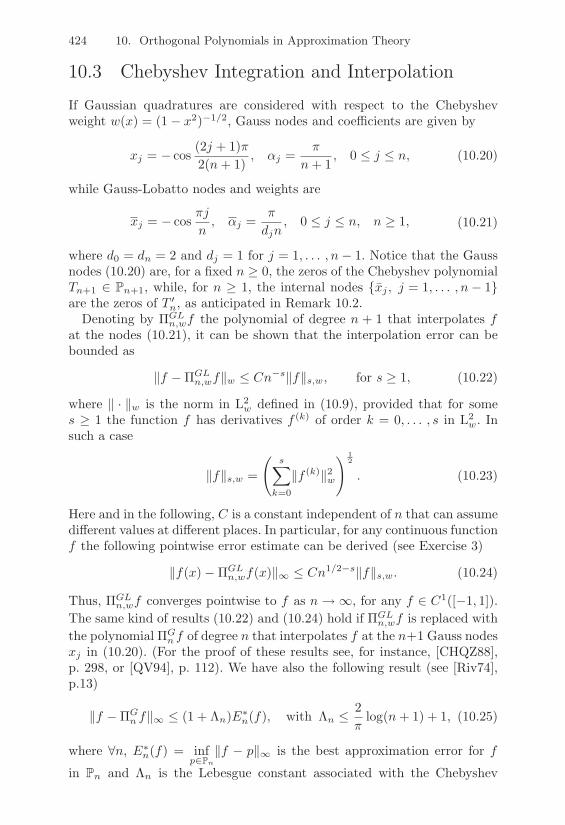
424 10. Orthogonal Polynomials in Approximation Theory
10.3 Chebyshev Integration and Interpolation
If Gaussian quadratures are considered with respect to the Chebyshevweight w(x) = (1" x2)"1/2, Gauss nodes and coe"cients are given by
xj = " cos(2j + 1)&2(n + 1)
, "j =&
n + 1, 0 & j & n, (10.20)
while Gauss-Lobatto nodes and weights are
xj = " cos&j
n, "j =
&
djn, 0 & j & n, n ) 1, (10.21)
where d0 = dn = 2 and dj = 1 for j = 1, . . . , n" 1. Notice that the Gaussnodes (10.20) are, for a fixed n ) 0, the zeros of the Chebyshev polynomialTn+1 ! Pn+1, while, for n ) 1, the internal nodes {xj , j = 1, . . . , n" 1}are the zeros of T *
n, as anticipated in Remark 10.2.Denoting by $GL
n,wf the polynomial of degree n + 1 that interpolates fat the nodes (10.21), it can be shown that the interpolation error can bebounded as
+f "$GLn,wf+w & Cn"s+f+s,w, for s ) 1, (10.22)
where + · +w is the norm in L2w defined in (10.9), provided that for some
s ) 1 the function f has derivatives f (k) of order k = 0, . . . , s in L2w. In
such a case
+f+s,w =
6s(
k=0
+f (k)+2w
7 12
. (10.23)
Here and in the following, C is a constant independent of n that can assumedi!erent values at di!erent places. In particular, for any continuous functionf the following pointwise error estimate can be derived (see Exercise 3)
+f(x)"$GLn,wf(x)+$ & Cn1/2"s+f+s,w. (10.24)
Thus, $GLn,wf converges pointwise to f as n(,, for any f ! C1(["1, 1]).
The same kind of results (10.22) and (10.24) hold if $GLn,wf is replaced with
the polynomial $Gn f of degree n that interpolates f at the n+1 Gauss nodes
xj in (10.20). (For the proof of these results see, for instance, [CHQZ88],p. 298, or [QV94], p. 112). We have also the following result (see [Riv74],p.13)
+f "$Gn f+$ & (1 + %n)E,
n(f), with %n &2&
log(n + 1) + 1, (10.25)
where #n, E,n(f) = inf
p#Pn
+f " p+$ is the best approximation error for f
in Pn and %n is the Lebesgue constant associated with the Chebyshev

10.3 Chebyshev Integration and Interpolation 425
nodes (10.20). As far as the numerical integration error is concerned, letus consider, for instance, the Gauss-Lobatto quadrature rule (10.18) withnodes and weights given in (10.21). First of all, notice that
1^
"1
f(x)(1" x2)"1/2dx = limn&$
IGLn,w(f)
for any function f whose left integral is finite (see [Sze67], p. 342). If,moreover, +f+s,w is finite for some s ) 1, we have
>>>>>>
1^
"1
f(x)(1" x2)"1/2dx" IGLn,w(f)
>>>>>>& Cn"s+f+s,w. (10.26)
This result follows from the more general one
|(f, vn)w " (f, vn)n| & Cn"s+f+s,w+vn+w, #vn ! Pn, (10.27)
where the so-called discrete scalar product has been introduced
(f, g)n =n(
j=0
"jf(xj)g(xj) = IGLn,w(fg). (10.28)
Actually, (10.26) follows from (10.27) setting vn ? 1 and noticing that
+vn+w =K@ 1
"1(1" x2)"1/2dxL1/2
=/&. Thanks to (10.26) we can thus
conclude that the (Chebyshev) Gauss-Lobatto formula has degree of ex-actness 2n " 1 and order of accuracy (with respect to n"1) equal to s,provided that +f+s,w <,. Therefore, the order of accuracy is only limitedby the regularity threshold s of the integrand function. Completely similarconsiderations can be drawn for (Chebyshev) Gauss formulae with n + 1nodes.Let us finally determine the coe"cients fk, k = 0, . . . , n, of the interpolat-ing polynomial $GL
n,wf at the n + 1 Gauss-Lobatto nodes in the expansionwith respect to the Chebyshev polynomials (10.10)
$GLn,wf(x) =
n(
k=0
fkTk(x). (10.29)
Notice that $GLn,wf coincides with the discrete truncation of the Chebyshev
series f,n defined in (10.4). Enforcing the equality $GL
n,wf(xj) = f(xj), j =0, . . . , n, we find
f(xj) =n(
k=0
cos4kj&
n
5fk, j = 0, . . . , n. (10.30)

426 10. Orthogonal Polynomials in Approximation Theory
Recalling the exactness of the Gauss-Lobatto quadrature, it can be checkedthat (see Exercise 2)
fk =2
ndk
n(
j=0
1dj
cos4kj&
n
5f(xj), k = 0, . . . , n. (10.31)
Relation (10.31) yields the discrete coe"cients {fk, k = 0, . . . , n} in termsof the nodal values {f(xj), j = 0, . . . , n}. For this reason it is calledthe Chebyshev discrete transform (CDT) and, thanks to its trigonomet-ric structure, it can be e"ciently computed using the FFT algorithm (FastFourier transform) with a number of floating-point operations of the orderof n log2 n (see Section 10.9.2). Of course, (10.30) is the inverse of the CDT,and can be computed using the FFT.
10.4 Legendre Integration and Interpolation
As previously noticed, the Legendre weight is w(x) ? 1. For n ) 0, theGauss nodes and the related coe"cients are given by
xj zeros of Ln+1(x), "j =2
(1" x2j )[L*
n+1(xj)]2, j = 0, . . . , n, (10.32)
while the Gauss-Lobatto ones are, for n ) 1
x0 = "1, xn = 1, xj zeros of L*n(x), j = 1, . . . , n" 1 (10.33)
"j =2
n(n + 1)1
[Ln(xj)]2, j = 0, . . . , n (10.34)
where Ln is the n-th Legendre polynomial defined in (10.12). It can bechecked that, for a suitable constant C independent of n,
2n(n + 1)
& "j &C
n, #j = 0, . . . , n
(see [BM92], p. 76). Then, letting $GLn f be the polynomial of degree n that
interpolates f at the n+1 nodes xj given by (10.33), it can be proved thatit fulfills the same error estimates as those reported in (10.22) and (10.24)in the case of the corresponding Chebyshev polynomial.
Of course, the norm + ·+w must here be replaced by the norm + ·+L2("1,1),while +f+s,w becomes
+f+s =
6s(
k=0
+f (k)+2L2("1,1)
7 12
. (10.35)

10.4 Legendre Integration and Interpolation 427
The same kinds of results are ensured if $GLn f is replaced by the polynomial
of degree n that interpolates f at the n + 1 nodes xj given by (10.32).Referring to the discrete scalar product defined in (10.28), but taking
now the nodes and coe"cients given by (10.33) and (10.34), we see that(·, ·)n is an approximation of the usual scalar product (·, ·) of L2("1, 1).Actually, the equivalent relation to (10.27) now reads
|(f, vn)" (f, vn)n| & Cn"s+f+s+vn+L2("1,1), #vn ! Pn (10.36)
and holds for any s ) 1 such that +f+s <,. In particular, setting vn ? 1,we get +vn+ =
/2, and from (10.36) it follows that
>>>>>>
1^
"1
f(x)dx" IGLn (f)
>>>>>>& Cn"s+f+s (10.37)
which demonstrates a convergence of the Gauss-Legendre-Lobatto quadra-ture formula to the exact integral of f with order of accuracy s with respectto n"1 provided that +f+s < ,. A similar result holds for the Gauss-Legendre quadrature formulae.
Example 10.1 Consider the approximate evaluation of the integral of f(x) =|x|!+ 3
5 over [%1, 1] for $ = 0, 1, 2. Notice that f has “piecewise” derivatives upto order s = s($) = $ + 1 in L2(%1, 1). Figure 10.1 shows the behavior of theerror as a function of n for the Gauss-Legendre quadrature formula. Accordingto (10.37), the convergence rate of the formula increases by one when $ increasesby one. •
100
101
102
103
10!10
10!8
10!6
10!4
10!2
100
102
FIGURE 10.1. The quadrature error in logarithmic scale as a function of n in thecase of a function with the first s derivatives in L2(%1, 1) for s = 1 (solid line),s = 2 (dashed line), s = 3 (dotted line)

428 10. Orthogonal Polynomials in Approximation Theory
The interpolating polynomial at the nodes (10.33) is given by
$GLn f(x) =
n(
k=0
fkLk(x). (10.38)
Notice that also in this case $GLn f coincides with the discrete truncation
of the Legendre series f,n defined in (10.4). Proceeding as in the previous
section, we get
f(xj) =n(
k=0
fkLk(xj), j = 0, . . . , n, (10.39)
and also
fk =
)****+
****,
2k + 1n(n + 1)
n(
j=0
Lk(xj)1
L2n(xj)
f(xj), k = 0, . . . , n" 1,
1n + 1
n(
j=0
1Ln(xj)
f(xj), k = n
(10.40)
(see Exercise 6). Formulae (10.40) and (10.39) provide, respectively, thediscrete Legendre transform (DLT) and its inverse.
10.5 Gaussian Integration over UnboundedIntervals
We consider integration on both half and on the whole of real axis. In bothcases we use interpolatory Gaussian formulae whose nodes are the zeros ofLaguerre and Hermite orthogonal polynomials, respectively.
The Laguerre polynomials. These are algebraic polynomials, orthogonalon the interval [0,+,) with respect to the weight function w(x) = e"x.They are defined by
Ln(x) = exdn
dxn(e"xxn), n ) 0,
and satisfy the following three-term recursive relationB
Ln+1(x) = (2n + 1" x)Ln(x)" n2Ln"1(x) n ) 0,
L"1 = 0, L0 = 1.
For any function f , define 1(x) = f(x)ex. Then, I(f) =@ $0 f(x)dx =@ $
0 e"x1(x)dx, so that it su"ces to apply to this last integral the Gauss-Laguerre quadratures, to get, for n ) 1 and f ! C2n([0,+,))
I(f) =n(
k=1
"k1(xk) +(n!)2
(2n)!1(2n)(*), 0 < * < +,, (10.41)

10.6 Programs for the Implementation of Gaussian Quadratures 429
where the nodes xk, for k = 1, . . . , n, are the zeros of Ln and the weightsare "k = (n!)2xk/[Ln+1(xk)]2. From (10.41), one concludes that Gauss-Laguerre formulae are exact for functions f of the type 1e"x, where 1 !P2n"1. In a generalized sense, we can then state that they have optimaldegrees of exactness equal to 2n" 1.
Example 10.2 Using a Gauss-Laguerre quadrature formula with n = 12 to com-pute the integral in Example 9.12 we obtain the value 0.5997 with an absoluteerror with respect to exact integration equal to 2.96 · 10%4. For the sake of com-parison, the composite trapezoidal formula would require 277 nodes to obtain thesame accuracy. •
The Hermite polynomials. These are orthogonal polynomials on thereal line with respect to the weight function w(x) = e"x2
. They are definedby
Hn(x) = ("1)nex2 dn
dxn(e"x2
), n ) 0.
Hermite polynomials can be recursively generated asB
Hn+1(x) = 2xHn(x)" 2nHn"1(x) n ) 0,
H"1 = 0, H0 = 1.
As in the previous case, letting 1(x) = f(x)ex2, we have I(f) =
@ $"$ f(x)dx =
@ $"$ e"x2
1(x)dx. Applying to this last integral the Gauss-Hermite quadra-tures we obtain, for n ) 1 and f ! C2n(R)
I(f) =$
"$
e"x21(x)dx =
n(
k=1
"k1(xk) +(n!)
/&
2n(2n)!1(2n)(*), * ! R,
(10.42)
where the nodes xk, for k = 1, . . . , n, are the zeros of Hn and the weightsare "k = 2n+1n!
/&/[Hn+1(xk)]2. As for Gauss-Laguerre quadratures, the
Gauss-Hermite rules also are exact for functions f of the form 1e"x2, where
1 ! P2n"1; therefore, they have optimal degrees of exactness equal to 2n"1.More details on the subject can be found in [DR75], pp. 173-174.
10.6 Programs for the Implementation of GaussianQuadratures
Programs 82, 83 and 84 compute the coe"cients {"k} and {#k}, introducedin (10.8), in the cases of the Legendre, Laguerre and Hermite polynomials.These programs are then called by Program 85 for the computation of nodes

430 10. Orthogonal Polynomials in Approximation Theory
and weights (10.32), in the case of the Gauss-Legendre formulae, and byPrograms 86, 87 for computing nodes and weights in the Gauss-Laguerreand Gauss-Hermite quadrature rules (10.41) and (10.42). All the codingsreported in this section are excerpts from the library ORTHPOL [Gau94].
Program 82 - coeflege : Coe"cients of Legendre polynomials
function [a, b] = coeflege(n)if (n <= 1), disp(’ n must be > 1 ’); return; endfor k=1:n, a(k)=0; b(k)=0; end; b(1)=2;for k=2:n, b(k)=1/(4-1/(k-1)ˆ2); end
Program 83 - coeflagu : Coe"cients of Laguerre polynomials
function [a, b] = coeflagu(n)if (n <= 1), disp(’ n must be > 1 ’); return; enda=zeros(n,1); b=zeros(n,1); a(1)=1; b(1)=1;for k=2:n, a(k)=2*(k-1)+1; b(k)=(k-1)ˆ2; end
Program 84 - coefherm : Coe"cients of Hermite polynomials
function [a, b] = coefherm(n)if (n <= 1), disp(’ n must be > 1 ’); return; enda=zeros(n,1); b=zeros(n,1); b(1)=sqrt(4.*atan(1.));for k=2:n, b(k)=0.5*(k-1); end
Program 85 - zplege : Coe"cients of Gauss-Legendre formulae
function [x,w]=zplege(n)if (n <= 1), disp(’ n must be > 1 ’); return; end[a,b]=coeflege(n);JacM=diag(a)+diag(sqrt(b(2:n)),1)+diag(sqrt(b(2:n)),-1);[w,x]=eig(JacM); x=diag(x); scal=2; w=w(1,:)’.ˆ2*scal;[x,ind]=sort(x); w=w(ind);
Program 86 - zplagu : Coe"cients of Gauss-Laguerre formulae
function [x,w]=zplagu(n)if (n <= 1), disp(’ n must be > 1 ’); return; end[a,b]=coeflagu(n);JacM=diag(a)+diag(sqrt(b(2:n)),1)+diag(sqrt(b(2:n)),-1);[w,x]=eig(JacM); x=diag(x); w=w(1,:)’.ˆ2;
Program 87 - zpherm : Coe"cients of Gauss-Hermite formulae
function [x,w]=zpherm(n)if (n <= 1), disp(’ n must be > 1 ’); return; end
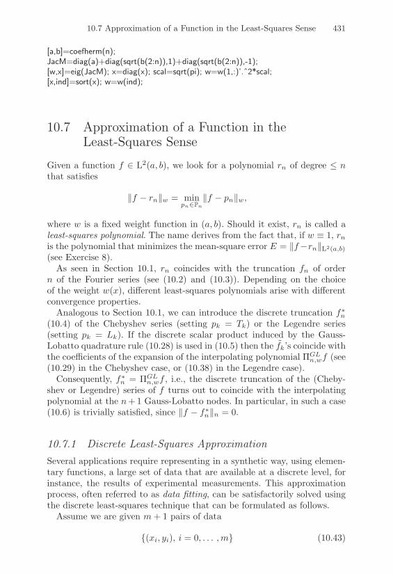
10.7 Approximation of a Function in the Least-Squares Sense 431
[a,b]=coefherm(n);JacM=diag(a)+diag(sqrt(b(2:n)),1)+diag(sqrt(b(2:n)),-1);[w,x]=eig(JacM); x=diag(x); scal=sqrt(pi); w=w(1,:)’.ˆ2*scal;[x,ind]=sort(x); w=w(ind);
10.7 Approximation of a Function in theLeast-Squares Sense
Given a function f ! L2(a, b), we look for a polynomial rn of degree & nthat satisfies
+f " rn+w = minpn#Pn
+f " pn+w,
where w is a fixed weight function in (a, b). Should it exist, rn is called aleast-squares polynomial. The name derives from the fact that, if w ? 1, rnis the polynomial that minimizes the mean-square error E = +f"rn+L2(a,b)(see Exercise 8).
As seen in Section 10.1, rn coincides with the truncation fn of ordern of the Fourier series (see (10.2) and (10.3)). Depending on the choiceof the weight w(x), di!erent least-squares polynomials arise with di!erentconvergence properties.
Analogous to Section 10.1, we can introduce the discrete truncation f,n
(10.4) of the Chebyshev series (setting pk = Tk) or the Legendre series(setting pk = Lk). If the discrete scalar product induced by the Gauss-Lobatto quadrature rule (10.28) is used in (10.5) then the fk’s coincide withthe coe"cients of the expansion of the interpolating polynomial $GL
n,wf (see(10.29) in the Chebyshev case, or (10.38) in the Legendre case).
Consequently, f,n = $GL
n,wf , i.e., the discrete truncation of the (Cheby-shev or Legendre) series of f turns out to coincide with the interpolatingpolynomial at the n+ 1 Gauss-Lobatto nodes. In particular, in such a case(10.6) is trivially satisfied, since +f " f,
n+n = 0.
10.7.1 Discrete Least-Squares ApproximationSeveral applications require representing in a synthetic way, using elemen-tary functions, a large set of data that are available at a discrete level, forinstance, the results of experimental measurements. This approximationprocess, often referred to as data fitting, can be satisfactorily solved usingthe discrete least-squares technique that can be formulated as follows.
Assume we are given m + 1 pairs of data
{(xi, yi), i = 0, . . . ,m} (10.43)
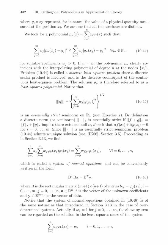
432 10. Orthogonal Polynomials in Approximation Theory
where yi may represent, for instance, the value of a physical quantity mea-sured at the position xi. We assume that all the abscissae are distinct.
We look for a polynomial pn(x) =n(
i=0
ai1i(x) such that
m(
j=0
wj |pn(xj)" yj |2 &m(
j=0
wj |qn(xj)" yj |2 #qn ! Pn, (10.44)
for suitable coe"cients wj > 0. If n = m the polynomial pn clearly co-incides with the interpolating polynomial of degree n at the nodes {xi}.Problem (10.44) is called a discrete least-squares problem since a discretescalar product is involved, and is the discrete counterpart of the contin-uous least-squares problem. The solution pn is therefore referred to as aleast-squares polynomial. Notice that
|||q||| =
)+
,
m(
j=0
wj [q(xj)]2
_`
a
1/2
(10.45)
is an essentially strict seminorm on Pn (see, Exercise 7). By definitiona discrete norm (or seminorm) + · +, is essentially strict if +f + g+, =+f+, + +g+, implies there exist nonnull ", # such that "f(xi)+#g(xi) = 0for i = 0, . . . ,m. Since ||| · ||| is an essentially strict seminorm, problem(10.44) admits a unique solution (see, [IK66], Section 3.5). Proceeding asin Section 3.13, we find
n(
k=0
ak
m(
j=0
wj1k(xj)1i(xj) =m(
j=0
wjyj1i(xj), #i = 0, . . . , n,
which is called a system of normal equations, and can be convenientlywritten in the form
BTBa = BTy, (10.46)
where B is the rectangular matrix (m+1)%(n+1) of entries bij = 1j(xi), i =0, . . . ,m, j = 0, . . . , n, a ! Rn+1 is the vector of the unknown coe"cientsand y ! Rm+1 is the vector of data.
Notice that the system of normal equations obtained in (10.46) is ofthe same nature as that introduced in Section 3.13 in the case of over-determined systems. Actually, if wj = 1 for j = 0, . . . ,m, the above systemcan be regarded as the solution in the least-squares sense of the system
n(
k=0
ak1k(xi) = yi, i = 0, 1, . . . ,m,

10.8 The Polynomial of Best Approximation 433
which would not admit a solution in the classical sense, since the number ofrows is greater than the number of columns. In the case n = 1, the solutionto (10.44) is a linear function, called linear regression for the data fittingof (10.43). The associated system of normal equations is
1(
k=0
m(
j=0
wj1i(xj)1k(xj)ak =m(
j=0
wj1i(xj)yj , i = 0, 1.
Setting (f, g)m =m(
j=0
f(xj)g(xj) the previous system becomes
B(10,10)ma0 + (11,10)ma1 = (y,10)m,
(10,11)ma0 + (11,11)ma1 = (y,11)m,
where y(x) is a function that takes the value yi at the nodes xi, i =0, . . . ,m. After some algebra, we get this explicit form for the coe"cients
a0 =(y,10)m(11,11)m " (y,11)m(11,10)m
(11,11)m(10,10)m " (10,11)2m,
a1 =(y,11)m(10,10)m " (y,10)m(11,10)m
(11,11)m(10,10)m " (10,11)2m.
Example 10.3 As already seen in Example 8.2, small changes in the data cangive rise to large variations on the interpolating polynomial of a given functionf . This doesn’t happen for the least-squares polynomial where m is much largerthan n. As an example, consider the function f(x) = sin(2+x) in [%1, 1] andevaluate it at the 22 equally spaced nodes xi = 2i/21, i = 0, . . . , 21, settingfi = f(xi). Then, suppose to add to the data fi a random perturbation of theorder of 10%3 and denote by p5 and p5 the least-squares polynomials of degree5 approximating the data fi and fi, respectively. The maximum norm of thedi"erence p5 % p5 over [%1, 1] is of the order of 10%3, i.e., it is of the same orderas the perturbation on the data. For comparison, the same di"erence in the caseof Lagrange interpolation is about equal to 2 as can be seen in Figure 10.2. •
10.8 The Polynomial of Best Approximation
Consider a function f ! C0([a, b]). A polynomial p,n ! Pn is said to be thepolynomial of best approximation of f if it satisfies
+f " p,n+$ = minpn#Pn
+f " pn+$, #pn ! Pn (10.47)
where +g+$ = maxa%x%b |g(x)|. This problem is referred to as a minimaxapproximation, as we are looking for the minimum error measured in themaximum norm.

434 10. Orthogonal Polynomials in Approximation Theory
!1 !0.5 0 0.5 1!2
!1.5
!1
!0.5
0
0.5
1
1.5
2
FIGURE 10.2. The perturbed data (circles), the associated least-squares polyno-mial of degree 5 (solid line) and the Lagrange interpolating polynomial (dashedline)
Property 10.1 (Chebyshev equioscillation theorem) For any n ) 0,the polynomial of best approximation p,n of f exists and is unique. More-over, in [a, b] there exist n + 2 points x0 < x1 < . . . < xn+1 such that
f(xj)" p,n(xj) = (("1)jE,n(f), j = 0, . . . , n + 1
with ( = 1 or ( = "1 depending on f and n, and E,n(f) = +f " p,n+$.
(For the proof, see [Dav63], Chapter 7). As a consequence, there exist n+1points x0 < x1 < . . . < xn, with xk < xk < xk+1 for k = 0, . . . , n, to bedetermined in [a, b] such that
p,n(xj) = f(xj), j = 0, 1, . . . , n,
so that the best approximation polynomial is a polynomial of degree n thatinterpolates f at n + 1 unknown nodes.
The following result yields an estimate of E,n(f) without explicitly com-
puting p,n (we refer for the proof to [Atk89], Chapter 4).
Property 10.2 (de la Vallee-Poussin theorem) Let n ) 0 and let x0 <x1 < . . . < xn+1 be n + 2 points in [a, b]. If there exists a polynomial qn ofdegree & n such that
f(xj)" qn(xj) = ("1)jej j = 0, 1, . . . , n + 1
where all ej have the same sign and are non null, then
min0%j%n+1
|ej | & E,n(f).
We can now relate E,n(f) with the interpolation error. Indeed,
+f "$nf+$ & +f " p,n+$ + +p,n "$nf+$.

10.9 Fourier Trigonometric Polynomials 435
On the other hand, using the Lagrange representation of p,n we get
+p,n "$nf+$ = +n(
i=0
(p,n(xi)" f(xi))li+$ & +p,n " f+$+n(
i=0
|li|+$,
from which it follows
+f "$nf+$ & (1 + %n)E,n(f),
where %n is the Lebesgue constant (8.11) associated with the nodes {xi}.Thanks to (10.25) we can conclude that the Lagrange interpolating poly-nomial on the Chebyshev nodes is a good approximation of p,n. The aboveresults yield a characterization of the best approximation polynomial, butdo not provide a constructive way for generating it. However, starting fromthe Chebyshev equioscillation theorem, it is possible to devise an algorithm,called the Remes algorithm, that is able to construct an arbitrarily goodapproximation of the polynomial p,n (see [Atk89], Section 4.7).
10.9 Fourier Trigonometric Polynomials
Let us apply the theory developed in the previous sections to a particularfamily of orthogonal polynomials which are no longer algebraic polynomialsbut rather trigonometric. The Fourier polynomials on (0, 2&) are definedas
1k(x) = eikx, k = 0,±1,±2, . . .
where i is the imaginary unit. These are complex-valued periodic functionswith period equal to 2&. We shall use the notation L2(0, 2&) to denote thecomplex-valued functions that are square integrable over (0, 2&). Therefore
L2(0, 2&) =Ef : (0, 2&) ( C such that
^ 2"
0|f(x)|2dx <,
F
with scalar product and norm defined respectively by
(f, g) =@ 2"0 f(x)g(x)dx, +f+L2(0,2") =
3(f, f).
If f ! L2(0, 2&), its Fourier series is
Ff =$(
k="$
:fk1k, with :fk =12&
2"^
0
f(x)e"ikxdx =12&
(f,1k). (10.48)
If f is complex-valued we set f(x) = "(x) + i#(x) for x ! [0, 2&], where"(x) is the real part of f and #(x) is the imaginary one. Recalling that

436 10. Orthogonal Polynomials in Approximation Theory
e"ikx = cos(kx)" i sin(kx) and letting
ak =12&
2"^
0
["(x) cos(kx) + #(x) sin(kx)] dx
bk =12&
2"^
0
[""(x) sin(kx) + #(x) cos(kx)] dx,
the Fourier coe"cients of the function f can be written as:fk = ak + ibk #k = 0,±1,±2, . . . . (10.49)
We shall assume henceforth that f is a real-valued function; in such a case:f"k = :fk for any k.
Let N be an even positive integer. Analogously to what was done inSection 10.1, we call the truncation of order N of the Fourier series thefunction
f,N (x) =
N2 "1(
k="N2
:fkeikx.
The use of capital N instead of small n is to conform with the notation usu-ally adopted in the analysis of discrete Fourier series (see [Bri74], [Wal91]).To simplify the notations we also introduce an index shift so that
f,N (x) =
N"1(
k=0
:fkei(k"N2 )x,
where now
:fk =12&
2"^
0
f(x)e"i(k"N/2)xdx =12&
(f, D1k), k = 0, . . . , N " 1 (10.50)
and D1k = e"i(k"N/2)x. Denoting by
SN = span{D1k, 0 & k & N " 1},
if f ! L2(0, 2&) its truncation of order N satisfies the following optimalapproximation property in the least-squares sense
+f " f,N+L2(0,2") = min
g#SN
+f " g+L2(0,2").
Set h = 2&/N and xj = jh, for j = 0, . . . , N " 1, and introduce thefollowing discrete scalar product
(f, g)N = hN"1(
j=0
f(xj)g(xj). (10.51)

10.9 Fourier Trigonometric Polynomials 437
Replacing (f, D1k) in (10.50) with (f, D1k)N , we get the discrete Fouriercoe"cients of the function f
Dfk =1N
N"1(
j=0
f(xj)e"ikjheij" =1N
N"1(
j=0
f(xj)W(k"N
2 )jN (10.52)
for k = 0, . . . , N " 1, where
WN = exp4"i2&
N
5
is the principal root of order N of unity. According to (10.4), the trigono-metric polynomial
$FNf(x) =
N"1(
k=0
Dfkei(k"N2 )x (10.53)
is called the discrete Fourier series of order N of f .
Lemma 10.1 The following property holds
(1l,1j)N = hN"1(
k=0
e"ik(l"j)h = 2&%jl, 0 & l, j & N " 1, (10.54)
where %jl is the Kronecker symbol.
Proof. For l = j the result is immediate. Thus, assume l $= j; we have that
N%1(
k=0
e%ik(l%j)h =1%
Ke%i(l%j)h
LN
1% e%i(l%j)h = 0.
Indeed, the numerator is 1 % (cos(2+(l % j))% i sin(2+(l % j))) = 1 % 1 = 0,while the denominator cannot vanish. Actually, it vanishes i" (j % l)h = 2+, i.e.,j % l = N , which is impossible. !
Thanks to Lemma 10.1, the trigonometric polynomial $FNf is the Fourier
interpolate of f at the nodes xj , that is
$FNf(xj) = f(xj), j = 0, 1, . . . , N " 1.
Indeed, using (10.52) and (10.54) in (10.53) it follows that
$FNf(xj) =
N"1(
k=0
Dfkeikjhe"ijhN2 =
N"1(
l=0
f(xl)
N1N
N"1(
k=0
e"ik(l"j)h
O
= f(xj).

438 10. Orthogonal Polynomials in Approximation Theory
Therefore, looking at the first and last equality, we get
f(xj) =N"1(
k=0
Dfkeik(j"N2 )h =
N"1(
k=0
DfkW"(j"N
2 )kN , j = 0, . . . , N " 1. (10.55)
The mapping {f(xj)} ( { Dfk} described by (10.52) is called the DiscreteFourier Transform (DFT), while the mapping (10.55) from { Dfk} to {f(xj)}is called the inverse transform (IDFT). Both DFT and IDFT can be writtenin matrix form as { Dfk} = T{f(xj)} and {f(xj)} = C{ Dfk} where T !CN!N , C denotes the inverse of T and
Tkj =1N
W(k"N
2 )jN , k, j = 0, . . . , N " 1,
Cjk = W"(j"N
2 )kN , j, k = 0, . . . , N " 1.
A naive implementation of the matrix-vector computation in the DFT andIDFT would require N2 operations. Using the FFT (Fast Fourier Trans-form) algorithm only O(N log2 N) flops are needed, provided that N is apower of 2, as will be explained in Section 10.9.2.
The function $FNf ! SN introduced in (10.53) is the solution of the
minimization problem +f " $FNf+N & +f " g+N for any g ! SN , where
+ · +N = (·, ·)1/2N is a discrete norm for SN . In the case where f is periodicwith all its derivatives up to order s (s ) 1), an error estimate analogousto that for Chebyshev and Legendre interpolation holds
+f "$FNf+L2(0,2") & CN"s+f+s
and alsomax
0%x%2"|f(x)"$F
Nf(x)| & CN1/2"s+f+s.
In a similar manner, we also have
|(f, vN )" (f, vN )N | & CN"s+f+s+vN+
for any vN ! SN , and in particular, setting vN = 1 we have the followingerror for the quadrature formula (10.51)
>>>>>>
2"^
0
f(x)dx" hN"1(
j=0
f(xj)
>>>>>>& CN"s+f+s
(see for the proof [CHQZ88], Chapter 2).
Notice that hN"1(
j=0
f(xj) is nothing else than the composite trapezoidal
rule for approximating the integral@ 2"0 f(x)dx. Therefore, such a formula

10.9 Fourier Trigonometric Polynomials 439
turns out to be extremely accurate when dealing with periodic and smoothintegrands.
Programs 88 and 89 provide an implementation of the DFT and IDFT. Theinput parameter f is a string containing the function f to be transformedwhile fc is a vector of size N containing the values Dfk.
Program 88 - dft : Discrete Fourier transform
function fc = dft(N,f)h = 2*pi/N; x=[0:h:2*pi*(1-1/N)]; fx = eval(f); wn = exp(-i*h);for k=0:N-1,
s = 0;for j=0:N-1
s = s + fx(j+1)*wnˆ((k-N/2)*j);endfc (k+1) = s/N;
end
Program 89 - idft : Inverse discrete Fourier transform
function fv = idft(N,fc)h = 2*pi/N; wn = exp(-i*h);for k=0:N-1
s = 0;for j=0:N-1
s = s + fc(j+1)*wnˆ(-k*(j-N/2));endfv (k+1) = s;
end
10.9.1 The Gibbs PhenomenonConsider the discontinuous function f(x) = x/& for x ! [0,&] and equal tox/&"2 for x ! (&, 2&], and compute its DFT using Program 88. The inter-polate $F
Nf is shown in Figure 10.3 (above) for N = 8, 16, 32. Notice thespurious oscillations around the point of discontinuity of f whose maximumamplitude, however, tends to a finite limit. The arising of these oscillationsis known as Gibbs phenomenon and is typical of functions with isolatedjump discontinuities; it a!ects the behavior of the truncated Fourier seriesnot only in the neighborhood of the discontinuity but also over the entireinterval, as can be clearly seen in the figure. The convergence rate of thetruncated series for functions with jump discontinuities is linear in N"1 atevery given non-singular point of the interval of definition of the function(see [CHQZ88], Section 2.1.4).

440 10. Orthogonal Polynomials in Approximation Theory
0 1 2 3 4 5 6
!1
!0.5
0
0.5
1
0 1 2 3 4 5 6!1
!0.5
0
0.5
1
FIGURE 10.3. Above: Fourier interpolate of the sawtooth function (thick solidline) for N = 8 (dash-dotted line), 16 (dashed line) and 32 (thin solid line).Below: the same informations are plotted in the case of the Lanczos smoothing
Since the Gibbs phenomenon is related to the slow decay of the Fouriercoe"cients of a discontinuous function, smoothing procedures can be prof-itably employed to attenuate the higher-order Fourier coe"cients. This canbe done by multiplying each coe"cient Dfk by a factor (k such that (k is adecreasing function of k. An example is provided by the Lanczos smoothing
(k =sin(2(k "N/2)(&/N))
2(k "N/2)(&/N), k = 0, . . . , N " 1. (10.56)
The e!ect of applying the Lanczos smoothing to the computation of theDFT of the above function f is represented in Figure 10.3 (below), whichshows that the oscillations have almost completely disappeared.
For a deeper analysis of this subject we refer to [CHQZ88], Chapter 2.
10.9.2 The Fast Fourier TransformAs pointed out in the previous section, computing the discrete Fouriertransform (DFT) or its inverse (IDFT) as a matrix-vector product, wouldrequire N2 operations. In this section we illustrate the basic steps of theCooley-Tukey algorithm [CT65], commonly known as Fast Fourier Trans-form (FFT). The computation of a DFT of order N is split into DFTs oforder p0, . . . , pm, where {pi} are the prime factors of N . If N is a power of2, the computational cost has the order of N log2 N flops.
A recursive algorithm to compute the DFT when N is a power of 2is described in the following. Let f = (fi)T , i = 0, . . . , N " 1 and set
p(x) = 1N
N"1(
j=0
fjxj . Then, computing the DFT of the vector f amounts to

10.9 Fourier Trigonometric Polynomials 441
evaluating p(W k"N2
N ) for k = 0, . . . , N"1. Let us introduce the polynomials
pe(x) =1N
Vf0 + f2x + . . . + fN"2x
N2 "1
W,
po(x) =1N
Vf1 + f3x + . . . + fN"1x
N2 "1
W.
Notice thatp(x) = pe(x2) + xpo(x2)
from which it follows that the computation of the DFT of f can be carriedout by evaluating the polynomials pe and po at the points W
2(k"N2 )
N , k =0, . . . , N " 1. Since
W2(k"N
2 )N = W 2k"N
N = exp4"i 2&k
N/2
5exp(i2&) = W k
N/2,
it turns out that we must evaluate pe and po at the principal roots of unityof order N/2. In this manner the DFT of order N is rewritten in termsof two DFTs of order N/2; of course, we can recursively apply again thisprocedure to po and pe. The process is terminated when the degree of thelast generated polynomials is equal to one.
In Program 90 we propose a simple implementation of the FFT recursivealgorithm. The input parameters are the vector f containing the NN valuesfk, where NN is a power of 2.
Program 90 - !trec : FFT algorithm in the recursive version
function [!tv]=!trec(f,NN)N = length(f); w = exp(-2*pi*sqrt(-1)/N);if N == 2!tv = f(1)+w.ˆ[-NN/2:NN-1-NN/2]*f(2);
elsea1 = f(1:2:N); b1 = f(2:2:N);a2 = !trec(a1,NN); b2 = !trec(b1,NN);for k=-NN/2:NN-1-NN/2!tv(k+1+NN/2) = a2(k+1+NN/2) + b2(k+1+NN/2)*wˆk;
endend
Remark 10.4 A FFT procedure can also be set up when N is not a powerof 2. The simplest approach consists of adding some zero samples to theoriginal sequence {fi} in such a way to obtain a total number of N = 2pvalues. This technique, however, does not necessarily yield the correct re-sult. Therefore, an e!ective alternative is based on partitioning the Fouriermatrix C into subblocks of smaller size. Practical FFT implementationscan handle both strategies (see, for instance, the fft package available inMATLAB). !

442 10. Orthogonal Polynomials in Approximation Theory
10.10 Approximation of Function Derivatives
A problem which is often encountered in numerical analysis is the ap-proximation of the derivative of a function f(x) on a given interval [a, b].A natural approach to it consists of introducing in [a, b] n + 1 nodes{xk, k = 0, . . . , n}, with x0 = a, xn = b and xk+1 = xk+h, k = 0, . . . , n"1where h = (b" a)/n. Then, we approximate f *(xi) using the nodal valuesf(xk) as
hm(
k="m
"kui"k =m%(
k="m%
#kf(xi"k), (10.57)
where {"k}, {#k} ! R are m+m* + 1 coe"cients to be determined and uk
is the desired approximation to f *(xk).A non negligible issue in the choice of scheme (10.57) is the computa-
tional e"ciency. Regarding this concern, it is worth noting that, if m '= 0,determining the values {ui} requires the solution of a linear system.
The set of nodes which are involved in constructing the derivative of f ata certain node, is called a stencil. The band of the matrix associated withsystem (10.57) increases as the stencil gets larger.
10.10.1 Classical Finite Di!erence MethodsThe simplest way to generate a formula like (10.57) consists of resorting tothe definition of the derivative. If f *(xi) exists, then
f *(xi) = limh&0+
f(xi + h)" f(xi)h
. (10.58)
Replacing the limit with the incremental ratio, with h finite, yields theapproximation
uFDi =
f(xi+1)" f(xi)h
, 0 & i & n" 1. (10.59)
Relation (10.59) is a special instance of (10.57) setting m = 0, "0 = 1,m* = 1, #"1 = 1, #0 = "1, #1 = 0.The right side of (10.59) is called the forward finite di!erence and theapproximation that is being used corresponds to replacing f *(xi) withthe slope of the straight line passing through the points (xi, f(xi)) and(xi+1, f(xi+1)), as shown in Figure 10.4.
To estimate the error that is made, it su"ces to expand f in Taylor’sseries, obtaining
f(xi+1) = f(xi) + hf *(xi) +h2
2f **(*i) with *i ! (xi, xi+1).

10.10 Approximation of Function Derivatives 443
We assume henceforth that f has the required regularity, so that
f *(xi)" uFDi = "h
2f **(*i). (10.60)
f(xi)
f(xi!1)f(xi+1)
xi!1 xi xi+1
FIGURE 10.4. Finite di"erence approximation of f ((xi): backward (solid line),forward (pointed line) and centred (dashed line)
Obviously, instead of (10.58) we could employ a centred incrementalratio, obtaining the following approximation
uCDi =
f(xi+1)" f(xi"1)2h
, 1 & i & n" 1. (10.61)
Scheme (10.61) is a special instance of (10.57) setting m = 0, "0 = 1,m* = 1, #"1 = 1/2, #0 = 0, #1 = "1/2.
The right side of (10.61) is called the centred finite di!erence and geometri-cally amounts to replacing f *(xi) with the slope of the straight line passingthrough the points (xi"1, f(xi"1)) and (xi+1, f(xi+1)) (see Figure 10.4).Resorting again to Taylor’s series, we get
f *(xi)" uCDi = "h2
6f ***(*i). (10.62)
Formula (10.61) thus provides a second-order approximation to f *(xi) withrespect to h.
Finally, with a similar procedure, we can derive a backward finite di!er-ence scheme, where
uBDi =
f(xi)" f(xi"1)h
, 1 & i & n, (10.63)

444 10. Orthogonal Polynomials in Approximation Theory
which is a!ected by the following error
f *(xi)" uBDi =
h
2f **(*i). (10.64)
The values of the parameters in (10.57) are m = 0, "0 = 1, m* = 1 and#"1 = 0, #0 = 1, #1 = "1.
Higher-order schemes, as well as finite di!erence approximations of higher-order derivatives of f , can be constructed using Taylor’s expansions ofhigher order. A remarkable example is the approximation of f **; if f !C4([a, b]) we easily get
f **(xi) =f(xi+1)" 2f(xi) + f(xi"1)
h2
"h2
24
Kf (4)(xi + !ih) + f (4)(xi " 0ih)
L, 0 < !i,0i < 1.
The following centred finite di!erence scheme can thus be derived
u**i =
f(xi+1)" 2f(xi) + f(xi"1)h2 , 1 & i & n" 1 (10.65)
which is a!ected by the error
f **(xi)" u**i = "h2
24
Kf (4)(xi + !ih) + f (4)(xi " 0ih)
L. (10.66)
Formula (10.65) provides a second-order approximation to f **(xi) with re-spect to h.
10.10.2 Compact Finite Di!erencesMore accurate approximations are provided by using the following formula(which we call compact di!erences)
"ui"1 + ui + "ui+1 =#
2h(fi+1 " fi"1) +
'
4h(fi+2 " fi"2) (10.67)
for i = 2, . . . , n" 1. We have set, for brevity, fi = f(xi).The coe"cients ", # and ' are to be determined in such a way that the
relations (10.67) yield values ui that approximate f *(xi) up to the highestorder with respect to h. For this purpose, the coe"cients are selected insuch a way as to minimize the consistency error (see Section 2.2)
(i(h) = "f (1)i"1 + f (1)
i " "f (1)i+1
"4#
2h(fi+1 " fi"1) +
'
4h(fi+2 " fi"2)
5 (10.68)

10.10 Approximation of Function Derivatives 445
which comes from “forcing” f to satisfy the numerical scheme (10.67). Forbrevity, we set f (k)
i = f (k)(xi), k = 1, 2, . . . .Precisely, assuming that f ! C5([a, b]) and expanding it in a Taylor’s
series around xi, we find
fi±1 = fi ± hf (1)i + h2
2 f (2)i ± h3
6 f (3)i + h4
24 f(4)i ± h5
120f(5)i + O(h6),
f (1)i±1 = f (1)
i ± hf (2)i + h2
2 f (3)i ± h3
6 f (4)i + h4
24 f(5)i + O(h5).
Substituting into (10.68) we get
(i(h) = (2"+ 1)f (1)i + "
h2
2f (3)i + "
h4
12f (5)i " (# + ')f (1)
i
"h2
2
4#
6+
2'3
5f (3)i " h4
60
4#
2+ 8'
5f (5)i + O(h6).
Second-order methods are obtained by equating to zero the coe"cient off (1)i , i.e., if 2"+1 = #+ ', while we obtain schemes of order 4 by equating
to zero also the coe"cient of f (3)i , yielding 6" = #+4' and finally, methods
of order 6 are obtained by setting to zero also the coe"cient of f (5)i , i.e.,
10" = # + 16'.The linear system formed by these last three equations has a nonsingularmatrix. Thus, there exists a unique scheme of order 6 that corresponds tothe following choice of the parameters
" = 1/3, # = 14/9, ' = 1/9, (10.69)
while there exist infinitely many methods of second and fourth order.Among these infinite methods, a popular scheme has coe"cients " = 1/4,# = 3/2 and ' = 0. Schemes of higher order can be generated at theexpense of furtherly expanding the computational stencil.
Traditional finite di!erence schemes correspond to setting " = 0 andallow for computing explicitly the approximant of the first derivative of fat a node, in contrast with compact schemes which are required in any caseto solve a linear system of the form Au = Bf (where the notation has theobvious meaning).To make the system solvable, it is necessary to provide values to the vari-ables ui with i < 0 and i > n. A particularly favorable instance is thatwhere f is a periodic function of period b " a, in which case ui+n = ui
for any i ! Z. In the nonperiodic case, system (10.67) must be suppliedby suitable relations at the nodes near the boundary of the approximationinterval. For example, the first derivative at x0 can be computed using therelation
u0 + "u1 =1h
(Af1 + Bf2 + Cf3 + Df4),
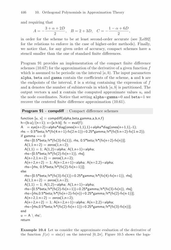
446 10. Orthogonal Polynomials in Approximation Theory
and requiring that
A = "3 + "+ 2D2
, B = 2 + 3D, C = "1" "+ 6D2
,
in order for the scheme to be at least second-order accurate (see [Lel92]for the relations to enforce in the case of higher-order methods). Finally,we notice that, for any given order of accuracy, compact schemes have astencil smaller than the one of standard finite di!erences.
Program 91 provides an implementation of the compact finite di!erenceschemes (10.67) for the approximation of the derivative of a given function fwhich is assumed to be periodic on the interval [a, b). The input parametersalpha, beta and gamma contain the coe"cients of the scheme, a and b arethe endpoints of the interval, f is a string containing the expression of fand n denotes the number of subintervals in which [a, b] is partitioned. Theoutput vectors u and x contain the computed approximate values ui andthe node coordinates. Notice that setting alpha=gamma=0 and beta=1 werecover the centered finite di!erence approximation (10.61).
Program 91 - compdi! : Compact di!erence schemes
function [u, x] = compdi!(alpha,beta,gamma,a,b,n,f)h=(b-a)/(n+1); x=[a:h:b]; fx = eval(f);A = eye(n+2)+alpha*diag(ones(n+1,1),1)+alpha*diag(ones(n+1,1),-1);rhs = 0.5*beta/h*(fx(4:n+1)-fx(2:n-1))+0.25*gamma/h*(fx(5:n+2)-fx(1:n-2));if gamma == 0
rhs=[0.5*beta/h*(fx(3)-fx(1)), rhs, 0.5*beta/h*(fx(n+2)-fx(n))];A(1,1:n+2) = zeros(1,n+2);A(1,1) = 1; A(1,2)=alpha; A(1,n+1)=alpha;rhs=[0.5*beta/h*(fx(2)-fx(n+1)), rhs];A(n+2,1:n+2) = zeros(1,n+2);A(n+2,n+2) = 1; A(n+2,n+1)=alpha; A(n+2,2)=alpha;rhs=[rhs, 0.5*beta/h*(fx(2)-fx(n+1))];
elserhs=[0.5*beta/h*(fx(3)-fx(1))+0.25*gamma/h*(fx(4)-fx(n+1)), rhs];A(1,1:n+2) = zeros(1,n+2);A(1,1) = 1; A(1,2)=alpha; A(1,n+1)=alpha;rhs=[0.5*beta/h*(fx(2)-fx(n+1))+0.25*gamma/h*(fx(3)-fx(n)), rhs];rhs=[rhs,0.5*beta/h*(fx(n+2)-fx(n))+0.25*gamma/h*(fx(2)-fx(n-1))];A(n+2,1:n+2) = zeros(1,n+2);A(n+2,n+2) = 1; A(n+2,n+1)=alpha; A(n+2,2)=alpha;rhs=[rhs,0.5*beta/h*(fx(2)-fx(n+1))+0.25*gamma/h*(fx(3)-fx(n))];
endu = A \ rhs’;return
Example 10.4 Let us consider the approximate evaluation of the derivative ofthe function f(x) = sin(x) on the interval [0, 2+]. Figure 10.5 shows the loga-

10.10 Approximation of Function Derivatives 447
rithm of the maximum nodal errors for the second-order centered finite di"er-ence scheme (10.61) and of the fourth and sixth-order compact di"erence schemesintroduced above, as a function of p = log(n). •
4 8 16 32 6410
!10
10!8
10!6
10!4
10!2
100
FIGURE 10.5. Maximum nodal errors for the second-order centred finite di"er-ence scheme (solid line) and for the fourth (dashed line) and sixth-order (dottedline) compact di"erence schemes as functions of p = log(n)
Another nice feature of compact schemes is that they maximize the rangeof well-resolved waves as we are going to explain. Assume that f is a realand periodic function on [0, 2&], that is, f(0) = f(2&). Using the samenotation as in Section 10.9, we let N be an even positive integer and seth = 2&/N . Then replace f by its truncated Fourier series
f,N (x) =
N/2"1(
k="N/2
:fkeikx.
Since the function f is real-valued, :fk = :f"k for k = 1, . . . , N/2 and:f0 = :f0. For sake of convenience, introduce the normalized wave numberwk = kh = 2&k/N and perform a scaling of the coordinates setting s = x/h.As a consequence, we get
f,N (x(s)) =
N/2"1(
k="N/2
:fkeiksh =N/2"1(
k="N/2
:fkeiwks. (10.70)
Taking the first derivative of (10.70) with respect to s yields a functionwhose Fourier coe"cients are :f *
k = iwk:fk. We can thus estimate the ap-
proximation error on (f,N )* by comparing the exact coe"cients :f *
k with thecorresponding ones obtained by an approximate derivative, in particular,by comparing the exact wave number wk with the approximate one, saywk,app.
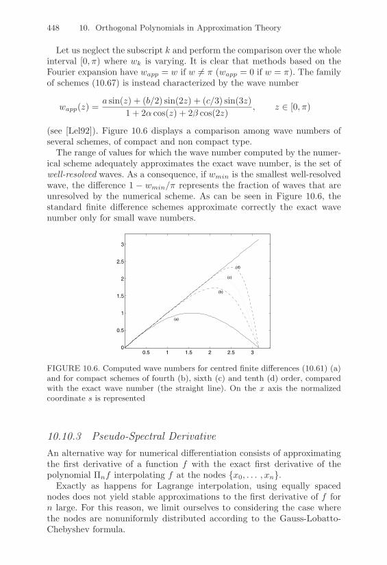
448 10. Orthogonal Polynomials in Approximation Theory
Let us neglect the subscript k and perform the comparison over the wholeinterval [0,&) where wk is varying. It is clear that methods based on theFourier expansion have wapp = w if w '= & (wapp = 0 if w = &). The familyof schemes (10.67) is instead characterized by the wave number
wapp(z) =a sin(z) + (b/2) sin(2z) + (c/3) sin(3z)
1 + 2" cos(z) + 2# cos(2z), z ! [0,&)
(see [Lel92]). Figure 10.6 displays a comparison among wave numbers ofseveral schemes, of compact and non compact type.
The range of values for which the wave number computed by the numer-ical scheme adequately approximates the exact wave number, is the set ofwell-resolved waves. As a consequence, if wmin is the smallest well-resolvedwave, the di!erence 1 " wmin/& represents the fraction of waves that areunresolved by the numerical scheme. As can be seen in Figure 10.6, thestandard finite di!erence schemes approximate correctly the exact wavenumber only for small wave numbers.
0.5 1 1.5 2 2.5 30
0.5
1
1.5
2
2.5
3
(a)
(b)
(c)
(d)
FIGURE 10.6. Computed wave numbers for centred finite di"erences (10.61) (a)and for compact schemes of fourth (b), sixth (c) and tenth (d) order, comparedwith the exact wave number (the straight line). On the x axis the normalizedcoordinate s is represented
10.10.3 Pseudo-Spectral DerivativeAn alternative way for numerical di!erentiation consists of approximatingthe first derivative of a function f with the exact first derivative of thepolynomial $nf interpolating f at the nodes {x0, . . . , xn}.
Exactly as happens for Lagrange interpolation, using equally spacednodes does not yield stable approximations to the first derivative of f forn large. For this reason, we limit ourselves to considering the case wherethe nodes are nonuniformly distributed according to the Gauss-Lobatto-Chebyshev formula.

10.10 Approximation of Function Derivatives 449
For simplicity, assume that I = [a, b] = ["1, 1] and for n ) 1, take inI the Gauss-Lobatto-Chebyshev nodes as in (10.21). Then, consider theLagrange interpolating polynomial $GL
n,wf , introduced in Section 10.3. Wedefine the pseudo-spectral derivative of f ! C0(I) to be the derivative ofthe polynomial $GL
n,wf
Dnf = ($GLn,wf)* ! Pn"1(I).
The error made in replacing f * with Dnf is of exponential type, that is, itonly depends on the smoothness of the function f . More precisely, thereexists a constant C > 0 independent of n such that
+f * "Dnf+w & Cn1"m+f+m,w, (10.71)
for any m ) 2 such that the norm +f+m,w, introduced in (10.23), is finite.Recalling (10.19) and using (10.27) yields
(Dnf)(xi) =n(
j=0
f(xj)l*j(xi), i = 0, . . . , n, (10.72)
so that the pseudo-spectral derivative at the interpolation nodes can becomputed knowing only the nodal values of f and of l*j . These values canbe computed once for all and stored in a matrix D ! R(n+1)!(n+1): Dij =l*j(xi) for i, j = 0, ..., n, called a pseudo-spectral di!erentiation matrix.
Relation (10.72) can thus be cast in matrix form as f * = Df , lettingf = [f(xi)] and f * = [(Dnf)(xi)] for i = 0, ..., n.The entries of D have the following explicit form (see [CHQZ88], p. 69)
Dlj =
)**********+
**********,
dldj
("1)l+j
xl " xj, l '= j,
"xj
2(1" x2j ), 1 & l = j & n" 1,
"2n2 + 16
, l = j = 0,
2n2 + 16
, l = j = n,
(10.73)
where the coe"cients dl have been defined in Section 10.3 (see also Example5.13 concerning the approximation of the multiple eigenvalue $ = 0 of D).To compute the pseudo-spectral derivative of a function f over the genericinterval [a, b], we only have to resort to the change of variables consideredin Remark 10.3.
The second-order pseudo-spectral derivative can be computed as theproduct of the matrix D and the vector f *, that is, f ** = Df *, or by di-rectly applying matrix D2 to the vector f .

450 10. Orthogonal Polynomials in Approximation Theory
10.11 Transforms and Their Applications
In this section we provide a short introduction to the most relevant integraltransforms and discuss their basic analytical and numerical properties.
10.11.1 The Fourier TransformDefinition 10.1 Let L1(R) denote the space of real or complex functionsdefined on the real line such that
$
"$
|f(t)| dt < +,.
For any f ! L1(R) its Fourier transform is a complex-valued functionF = F [f ] defined as
F (3) =$
"$
f(t)e"i2".t dt.
!
Should the independent variable t denote time, then 3 would have themeaning of frequency. Thus, the Fourier transform is a mapping that to afunction of time (typically, real-valued) associates a complex-valued func-tion of frequency.The following result provides the conditions under which an inversion for-mula exists that allows us to recover the function f from its Fourier trans-form F (for the proof see [Rud83], p. 199).
Property 10.3 (inversion theorem) Let f be a given function in L1(R),F ! L1(R) be its Fourier transform and g be the function defined by
g(t) =$
"$
F (3)ei2".t d3, t ! R. (10.74)
Then g ! C0(R), with lim|x|&$ g(x) = 0, and f(t) = g(t) almost every-where in R (i.e., for any t unless possibly a set of zero measure).
The integral at right hand side of (10.74) is to be meant in the Cauchyprincipal value sense, i.e., we let
$
"$
F (3)ei2".t d3 = lima&$
a^
"a
F (3)ei2".t d3

10.11 Transforms and Their Applications 451
and we call it the inverse Fourier transform or inversion formula of theFourier transform. This mapping that associates to the complex functionF the generating function f will be denoted by F"1[F ], i.e., F = F [f ] i!f = F"1[F ].Let us briefly summarize the main properties of the Fourier transform andits inverse.
1. F and F"1 are linear operators, i.e.
F ["f + #g] = "F [f ] + #F [g], #",# ! C,
F"1["F + #G] = "F"1[F ] + #F"1[G], #",# ! C;(10.75)
2. scaling: if " is any nonzero real number and f! is the function f!(t) =f("t), then
F [f!] =1|"|F
1"
where F 1"(3) = F (3/");
3. duality: let f(t) be a given function and F (3) be its Fourier trans-form. Then the function g(t) = F ("t) has a Fourier transform givenby f(3). Thus, once an associated function-transform pair is found,another dual pair is automatically generated. An application of thisproperty is provided by the pair r(t)-F [r] in Example 10.5;
4. parity: if f(t) is a real even function then F (3) is real and even, whileif f(t) is a real and odd function then F (3) is imaginary and odd.This property allows one to work only with nonnegative frequencies;
5. convolution and product: for any given functions f, g ! L1(R), wehave
F [f @ g] = F [f ]F [g], F [fg] = F @G, (10.76)
where the convolution integral of two functions 4 and 6 is given by
(4 @ 6)(t) =$
"$
4(5)6(t" 5) d5. (10.77)
Example 10.5 We provide two examples of the computation of the Fouriertransforms of functions that are typically encountered in signal processing.Let us first consider the square wave (or rectangular) function r(t) defined as
r(t) =
BA if % T
2 " t " T2 ,
0 otherwise,

452 10. Orthogonal Polynomials in Approximation Theory
where T and A are two given positive numbers. Its Fourier transform F [r] is thefunction
F (2) =
T/2^
%T/2
Ae%i2)+t dt = ATsin(+2T )
+2T, 2 / R
where AT is the area of the rectangular function.Let us consider the sawtooth function
s(t) =
)+
,
2AtT
if % T2 " t " T
2 ,
0 otherwise,
whose DFT is shown in Figure 10.3 and whose Fourier transform F [s] is thefunction
F (2) = iAT+2T
-cos(+2T )% sin(+2T )
+2T
., 2 / R
and is purely imaginary since s is an odd real function. Notice also that thefunctions r and s have a finite support whereas their transforms have an infinitesupport (see Figure 10.7). In signal theory this corresponds to saying that thetransform has an infinite bandwidth. •
!10 !8 !6 !4 !2 0 2 4 6 8 10!0.4
!0.2
0
0.2
0.4
0.6
0.8
1
, !10 !8 !6 !4 !2 0 2 4 6 8 10!0.5
!0.4
!0.3
!0.2
!0.1
0
0.1
0.2
0.3
0.4
0.5
FIGURE 10.7. Fourier transforms of the rectangular (left) and the sawtooth(right) functions
Example 10.6 The Fourier transform of a sinusoidal function is of paramountinterest in signal and communication systems. To start with, consider the constantfunction f(t) = A for a given A / R. Since it has an infinite time duration itsFourier transform F [A] is the function
F (2) = lima$!
a^
%a
Ae%i2)+t dt = A lima$!
sin(2+2a)+2
,
where the integral above is again the Cauchy principal value of the correspondingintegral over (%#,#). It can be proved that the limit exists and is unique in thesense of distributions (see Section 12.4) yielding
F (2) = A!(2), (10.78)
10.11 Transforms and Their Applications 453
where ! is the so-called Dirac mass, i.e., a distribution that satisfies^ !
%!!(/)3(/) d/ = 3(0) (10.79)
for any function 3 continuous at the origin. From (10.78) we see that the trans-form of a function with infinite time duration has a finite bandwidth.
Let us now consider the computation of the Fourier transform of the functionf(t) = A cos(2+20t) where 20 is a fixed frequency. Recalling Euler’s formula
cos(.) =ei# + e%i#
2, . / R,
and applying (10.78) twice we get
F [A cos(2+20t)] =A2!(2 % 20) +
A2!(2 + 20),
which shows that the spectrum of a sinusoidal function with frequency 20 iscentred around ±20 (notice that the transform is even and real since the sameholds for the function f(t)). •
It is worth noting that in real-life there do not exist functions (i.e. signals)with infinite duration or bandwidth. Actually, if f(t) is a function whosevalue may be considered as “negligible” outside of some interval (ta, tb),then we can assume that the e!ective duration of f is the length #t =tb " ta. In a similar manner, if F (3) is the Fourier transform of f andit happens that F (3) may be considered as “negligible” outside of someinterval (3a, 3b), then the e!ective bandwidth of f is #3 = 3b"3a. Referringto Figure 10.7, we clearly see that the e!ective bandwidth of the rectangularfunction can be taken as ("10, 10).
10.11.2 (Physical) Linear Systems and Fourier TransformMathematically speaking, a physical linear system (LS) can be regardedas a linear operator S that enjoys the linearity property (10.75). Denotingby i(t) and u(t) an admissible input function for S and its correspondingoutput function respectively, the LS can be represented as u(t) = S(i(t))or S : i ( u. A special category of LS are the so-called shift invariant (ortime-invariant) linear systems (ILS) which satisfy the property
S(i(t" t0)) = u(t" t0), #t0 ! R
and for any admissible input function i.Let S be an ILS system and let f and g be two admissible input functions
for S with w = S(g). An immediate consequence of the linearity and shift-invariance is that
S((f @ g)(t)) = (f @ S(g))(t) = (f @ w)(t) (10.80)

454 10. Orthogonal Polynomials in Approximation Theory
where @ is the convolution operator defined in (10.77).Assume we take as input function the impulse function %(t) introduced in
the previous section and denote by h(t) = S(%(t)) the corresponding outputthrough S (usually referred to as the system impulse response function).Property (10.79) implies that for any function 4, (4 @ %)(t) = 4(t), so that,recalling (10.80) and taking 4(t) = i(t) we have
u(t) = S(i(t)) = S(i @ %)(t) = (i @ S(%))(t) = (i @ h)(t).
Thus, S can be completely described through its impulse response function.Equivalently, we can pass to the frequency domain by means of the firstrelation in (10.76) obtaining
U(3) = I(3)H(3), (10.81)
where I, U and H are the Fourier transforms of i(t), u(t) and h(t), respec-tively; H is the so-called system transfer function.
Relation (10.81) plays a central role in the analysis of linear time-invariantsystems as it is simpler to deal with the system transfer function than withthe corresponding impulse response function, as demonstrated in the fol-lowing example.
Example 10.7 (ideal low-pass filter) An ideal low-pass filter is an ILS char-acterized by the transfer function
H(2) =E
1, if |2| " 20/2,0, otherwise.
Using the duality property, the impulse response function F%1[H] is
h(t) = 20sin(+20t)
+20t.
Given an input signal i(t) with Fourier transform I(2), the corresponding outputu(t) has a spectrum given by (10.81)
I(2)H(2) =E
I(2), if |2| " 20/2,0 otherwise.
The e"ect of the filter is to cut o" the input frequencies that lie outside thewindow |2| " 20/2. •
The input/output functions i(t) and u(t) usually denote signals andthe linear system described by H(3) is typically a communication system.Therefore, as pointed out at the end of Section 10.11.1, we are legitimatedin assuming that both i(t) and u(t) have a finite e!ective duration. In

10.11 Transforms and Their Applications 455
particular, referring to i(t) we suppose i(t) = 0 if t '! [0, T0). Then, thecomputation of the Fourier transform of i(t) yields
I(3) =T0^
0
i(t)e"i2".t dt.
Letting #t = T0/n for n ) 1 and approximating the integral above by thecomposite trapezoidal formula (9.14), we get
I(3) = #tn"1(
k=0
i(k#t)e"i2".k!t.
It can be proved (see, e.g., [Pap62]) that I(3)/#t is the Fourier transformof the so-called sampled signal
is(t) =$(
k="$i(k#t)%(t" k#t),
where %(t " k#t) is the Dirac mass at k#t. Then, using the convolutionand the duality properties of the Fourier transform, we get
I(3) =$(
j="$I
43 " j
#t
5, (10.82)
which amounts to replacing I(3) by its periodic repetition with period1/#t. Let J!t = [" 1
2!t ,1
2!t ]; then, it su"ces to compute (10.82) for 3 !J!t. This can be done numerically by introducing a uniform discretizationof J!t with frequency step 30 = 1/(m#t) for m ) 1. By doing so, thecomputation of I(3) requires evaluating the following m+1 discrete Fouriertransforms (DFT)
I(j30) = #tn"1(
k=0
i(k#t)e"i2"j.0k!t, j = "m2 , . . . ,
m2 .
For an e"cient computation of each DFT in the formula above it is crucialto use the FFT algorithm described in Section 10.9.2.
10.11.3 The Laplace TransformThe Laplace transform can be employed to solve ordinary di!erential equa-tions with constant coe"cients as well as partial di!erential equations.
Definition 10.2 Let f ! L1loc([0,,)) i.e., f ! L1([0, T ]) for any T > 0.
Let s = ( + i0 be a complex variable. The Laplace integral of f is defined
456 10. Orthogonal Polynomials in Approximation Theory
as
$
0
f(t)e"st dt = limT&$
T
0
f(t)e"st dt.
If this integral exists for some s, it turns out to be a function of s; then,the Laplace transform L[f ] of f is the function
L(s) =$
0
f(t)e"st dt.
!
The following relation between Laplace and Fourier transforms holds
L(s) = F (e"$tf(t)),
where f(t) = f(t) if t ) 0 while f(t) = 0 if t < 0.
Example 10.8 The Laplace transform of the unit step function f(t) = 1 if t > 0,f(t) = 0 otherwise, is given by
L(s) =!
0
e%st dt =1s.
We notice that the Laplace integral exists if ' > 0. •
In Example 10.8 the convergence region of the Laplace integral is the half-plane {Re(s) > 0} of the complex field. This property is quite general, asstated by the following result.
Property 10.4 If the Laplace transform exists for s = s then it existsfor all s with Re(s) > Re(s). Moreover, let E be the set of the real partsof s such that the Laplace integral exists and denote by $ the infimum ofE. If $ happens to be finite, the Laplace integral exists in the half-planeRe(s) > $. If $ = ", then it exists for all s ! C; $ is called the abscissaof convergence.
We recall that the Laplace transform enjoys properties completely analo-gous to those of the Fourier transform. The inverse Laplace transform isdenoted formally as L"1 and is such that
f(t) = L"1[L(s)].
10.11 Transforms and Their Applications 457
Example 10.9 Let us consider the ordinary di"erential equation y((t)+ay(t) =g(t) with y(0) = y0. Multiplying by est, integrating between 0 and# and passingto the Laplace transform, yields
sY (s)% y0 + aY (s) = G(s). (10.83)
Should G(s) be easily computable, (10.83) would furnish Y (s) and then, by ap-plying the inverse Laplace transform, the generating function y(t). For instance,if g(t) is the unit step function, we obtain
y(t) = L%1E
1a
-1s% 1
s + a
.+
y0
s + a
F=
1a(1% e%at) + y0e
%at.
•
For an extensive presentation and analysis of the Laplace transform see,e.g., [Tit37]. In the next section we describe a discrete version of the Laplacetransform, known as the Z-transform.
10.11.4 The Z-TransformDefinition 10.3 Let f be a given function, defined for any t ) 0, and#t > 0 be a given time step. The function
Z(z) =$(
n=0
f(n#t)z"n, z ! C (10.84)
is called the Z-transform of the sequence {f(n#t)} and is denoted byZ[f(n#t)]. !
The parameter #t is the sampling time step of the sequence of samplesf(n#t). The infinite sum (10.84) converges if
|z| > R = lim supn&$
n3|f(n#t)|.
It is possible to deduce the Z-transform from the Laplace transform asfollows. Denoting by f0(t) the piecewise constant function such that f0(t) =f(n#t) for t ! (n#t, (n + 1)#t), the Laplace transform L[f0] of f0 is thefunction
L(s) =$
0
f0(t)e"st dt =$(
n=0
(n+1)!t^
n!t
e"stf(n#t) dt
=$(
n=0
f(n#t)e"ns!t " e"(n+1)s!t
s=
41" e"s!t
s
5 $(
n=0
f(n#t)e"ns!t.
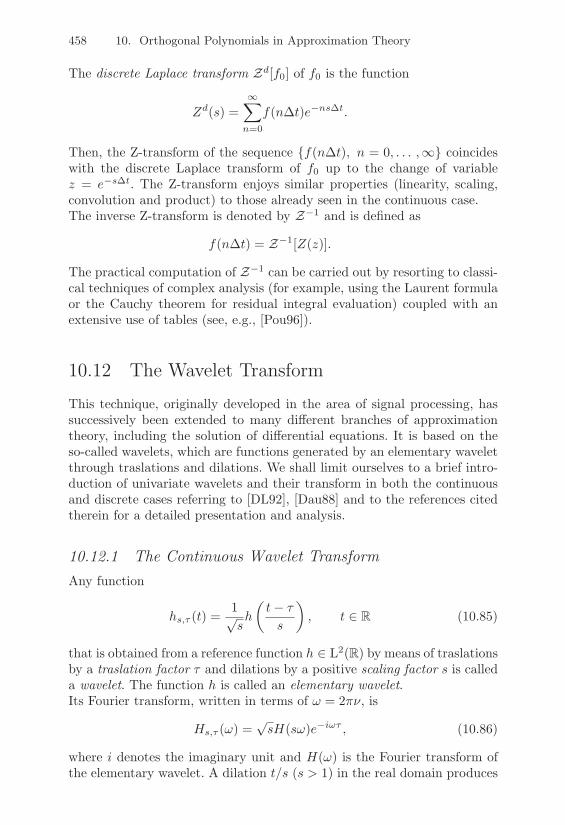
458 10. Orthogonal Polynomials in Approximation Theory
The discrete Laplace transform Zd[f0] of f0 is the function
Zd(s) =$(
n=0
f(n#t)e"ns!t.
Then, the Z-transform of the sequence {f(n#t), n = 0, . . . ,,} coincideswith the discrete Laplace transform of f0 up to the change of variablez = e"s!t. The Z-transform enjoys similar properties (linearity, scaling,convolution and product) to those already seen in the continuous case.The inverse Z-transform is denoted by Z"1 and is defined as
f(n#t) = Z"1[Z(z)].
The practical computation of Z"1 can be carried out by resorting to classi-cal techniques of complex analysis (for example, using the Laurent formulaor the Cauchy theorem for residual integral evaluation) coupled with anextensive use of tables (see, e.g., [Pou96]).
10.12 The Wavelet Transform
This technique, originally developed in the area of signal processing, hassuccessively been extended to many di!erent branches of approximationtheory, including the solution of di!erential equations. It is based on theso-called wavelets, which are functions generated by an elementary waveletthrough traslations and dilations. We shall limit ourselves to a brief intro-duction of univariate wavelets and their transform in both the continuousand discrete cases referring to [DL92], [Dau88] and to the references citedtherein for a detailed presentation and analysis.
10.12.1 The Continuous Wavelet TransformAny function
hs,/ (t) =1/sh
4t" 5s
5, t ! R (10.85)
that is obtained from a reference function h ! L2(R) by means of traslationsby a traslation factor 5 and dilations by a positive scaling factor s is calleda wavelet. The function h is called an elementary wavelet.Its Fourier transform, written in terms of 0 = 2&3, is
Hs,/ (0) =/sH(s0)e"i*/ , (10.86)
where i denotes the imaginary unit and H(0) is the Fourier transform ofthe elementary wavelet. A dilation t/s (s > 1) in the real domain produces

10.12 The Wavelet Transform 459
therefore a contraction s0 in the frequency domain. Therefore, the factor1/s plays the role of the frequency 3 in the Fourier transform (see Section10.11.1). In wavelets theory s is usually referred to as the scale. Formula(10.86) is known as the filter of the wavelet transform.
Definition 10.4 Given a function f ! L2(R), its continuous wavelet trans-form Wf = W[f ] is a decomposition of f(t) onto a wavelet basis {hs,/ (t)},that is
Wf (s, 5) =$
"$
f(t)hs,/ (t) dt, (10.87)
where the overline bar denotes complex conjugate. !When t denotes the time-variable, the wavelet transform of f(t) is a func-tion of the two variables s (scale) and 5 (time shift); as such, it is a repre-sentation of f in the time-scale space and is usually referred to as time-scalejoint representation of f . The time-scale representation is the analogue ofthe time-frequency representation introduced in the Fourier analysis. Thislatter representation has an intrinsic limitation: the product of the res-olution in time #t and the resolution in frequency #0 must satisfy thefollowing constraint (Heisenberg inequality)
#t#0 ) 12
(10.88)
which is the counterpart of the Heisenberg uncertainty principle in quantummechanics. This inequality states that a signal cannot be represented asa point in the time-frequency space. We can only determine its positionwithin a rectangle of area #t#0 in the time-frequency space.
The wavelet transform (10.87) can be rewritten in terms of the Fouriertransform F (0) of f as
Wf (s, 5) =/s
2&
$
"$
F (0)H(s0)ei*/ d0,
which shows that the wavelets transform is a bank of wavelet filters char-acterized by di!erent scales. More precisely, if the scale is small the waveletis concentrated in time and the wavelet transform provides a detailed de-scription of f(t) (which is the signal). Conversely, if the scale is large, thewavelet transform is able to resolve only the large-scale details of f . Thus,the wavelet transform can be regarded as a bank of multiresolution filters.
The theoretical properties of this transform do not depend on the partic-ular elementary wavelet that is considered. Hence, specific bases of waveletscan be derived for specific applications. Some examples of elementary wave-lets are reported below.

460 10. Orthogonal Polynomials in Approximation Theory
Example 10.10 (Haar wavelets) These functions can be obtained by choos-ing as the elementary wavelet the Haar function defined as
h(x) =
)+
,
1 if x / (0, 12 ),
%1 if x / ( 12 , 1),
0 otherwise.
Its Fourier transform is the complex-valued function
H(-) = 4ie%i,/2K1% cos(
-2
)L/-,
which has symmetric module with respect to the origin (see Figure 10.8). Thebases that are obtained from this wavelet are not used in practice due to theirine"ective localization properties in the frequency domain. •
!0.5 0 0.5 1 1.5!1.5
!1
!0.5
0
0.5
1
1.5
!80 !60 !40 !20 0 20 40 60 800
0.5
1
1.5
FIGURE 10.8. The Haar wavelet (left) and the module of its Fourier transform(right)
Example 10.11 (Morlet wavelets) The Morlet wavelet is defined as follows(see [MMG87])
h(x) = ei,0xe%x2/2.
Thus, it is a complex-valued function whose real part has a real positive Fouriertransform, symmetric with respect to the origin, given by
H(-) ='+
Ve%(,%,0)2/2 + e%(,+,0)2/2
W.
•
We point out that the presence of the dilation factor allows for the waveletsto easily handle possible discontinuities or singularities in f . Indeed, usingthe multi-resolution analysis, the signal, properly divided into frequencybandwidths, can be processed at each frequency by suitably tuning up thescale factor of the wavelets.
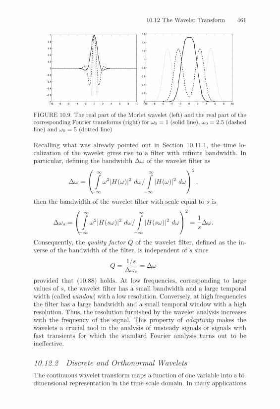
10.12 The Wavelet Transform 461
!10 !8 !6 !4 !2 0 2 4 6 8 10!1
!0.8
!0.6
!0.4
!0.2
0
0.2
0.4
0.6
0.8
1
!10 !8 !6 !4 !2 0 2 4 6 8 100
0.2
0.4
0.6
0.8
1
1.2
1.4
1.6
FIGURE 10.9. The real part of the Morlet wavelet (left) and the real part of thecorresponding Fourier transforms (right) for -0 = 1 (solid line), -0 = 2.5 (dashedline) and -0 = 5 (dotted line)
Recalling what was already pointed out in Section 10.11.1, the time lo-calization of the wavelet gives rise to a filter with infinite bandwidth. Inparticular, defining the bandwidth #0 of the wavelet filter as
#0 =
G
H$
"$
02|H(0)|2 d0/
$
"$
|H(0)|2 d0
I
J2
,
then the bandwidth of the wavelet filter with scale equal to s is
#0s =
G
H$
"$
02|H(s0)|2 d0/
$
"$
|H(s0)|2 d0
I
J2
=1s#0.
Consequently, the quality factor Q of the wavelet filter, defined as the in-verse of the bandwidth of the filter, is independent of s since
Q =1/s#0s
= #0
provided that (10.88) holds. At low frequencies, corresponding to largevalues of s, the wavelet filter has a small bandwidth and a large temporalwidth (called window) with a low resolution. Conversely, at high frequenciesthe filter has a large bandwidth and a small temporal window with a highresolution. Thus, the resolution furnished by the wavelet analysis increaseswith the frequency of the signal. This property of adaptivity makes thewavelets a crucial tool in the analysis of unsteady signals or signals withfast transients for which the standard Fourier analysis turns out to beine!ective.
10.12.2 Discrete and Orthonormal WaveletsThe continuous wavelet transform maps a function of one variable into a bi-dimensional representation in the time-scale domain. In many applications

462 10. Orthogonal Polynomials in Approximation Theory
this description is excessively rich. Resorting to the discrete wavelets isan attempt to represent a function using a finite (and small) number ofparameters.
A discrete wavelet is a continuous wavelet that is generated by usingdiscrete scale and translation factors. For s0 > 1, denote by s = sj0 thescale factors; the dilation factors usually depend on the scale factors bysetting 5 = k50s
j0, 50 ! R. The corresponding discrete wavelet is
hj,k(t) = s"j/20 h(s"j
0 (t" k50sj0)) = s"j/2
0 h(s"j0 t" k50).
The scale factor sj0 corresponds to the magnification or the resolution ofthe observation, while the translation factor 50 is the location where theobservations are made. If one looks at very small details, the magnificationmust be large, which corresponds to large negative index j. In this case thestep of translation is small and the wavelet is very concentrated around theobservation point. For large and positive j, the wavelet is spread out andlarge translation steps are used.
The behavior of the discrete wavelets depends on the steps s0 and 50.When s0 is close to 1 and 50 is small, the discrete wavelets are close to thecontinuous ones. For a fixed scale s0 the localization points of the discretewavelets along the scale axis are logarithmic as log s = j log s0. The choices0 = 2 corresponds to the dyadic sampling in frequency. The discrete time-step is 50sj0 and, typically, 50 = 1. Hence, the time-sampling step is afunction of the scale and along the time axis the localization points of thewavelet depend on the scale.
For a given function f ! L1(R), the corresponding discrete wavelet trans-form is
Wf (j, k) =$
"$
f(t)hj,k(t) dt.
It is possible to introduce an orthonormal wavelet basis using discrete di-lation and traslation factors, i.e.
$
"$
hi,j hk,l(t) dt = %ik%jl, #i, j, k, l ! Z.
With an orthogonal wavelet basis, an arbitrary function f can be recon-structed by the expansion
f(t) = A(
j,k#Z
Wf (j, k)hj,k(t),
where A is a constant that does not depend on f .As of the computational standpoint, the wavelet discrete transform can
be implemented at even a cheaper cost than the FFT algorithm for com-puting the Fourier transform.

10.13 Applications 463
10.13 Applications
In this section we apply the theory of orthogonal polynomials to solve twoproblems arising in quantum physics. In the first example we deal withGauss-Laguerre quadratures, while in the second case the Fourier analysisand the FFT are considered.
10.13.1 Numerical Computation of Blackbody RadiationThe monochromatic energy density E(3) of blackbody radiation as a func-tion of frequency 3 is expressed by the following law
E(3) =8&hc3
33
eh./KBT " 1,
where h is the Planck constant, c is the speed of light, KB is the Boltz-mann constant and T is the absolute temperature of the blackbody (see,for instance, [AF83]).
To compute the total density of monochromatic energy that is emittedby the blackbody (that is, the emitted energy per unit volume) we mustevaluate the integral
E =$
0
E(3)d3 = "T 4
$
0
x3
ex " 1dx,
where x = h3/KBT and " = (8&K4B)/(ch)3 1 1.16 · 10"16 [J ][K"4][m"3].
We also let f(x) = x3/(ex " 1) and I(f) =@ $0 f(x)dx.
To approximate I(f) up to a previously fixed absolute error & %, we com-pare method 1. introduced in Section 9.8.3 with Gauss-Laguerre quadra-tures.In the case of method 1. we proceed as follows. For any a > 0 we letI(f) =
@ a0 f(x)dx +
@ $a f(x)dx and try to find a function 4 such that
$
a
f(x)dx &$
a
4(x)dx & %
2, (10.89)
the integral@ $a 4(x)dx being “easy” to compute. Once the value of a
has been found such that (10.89) is fulfilled, we compute the integralI1(f) =
@ a0 f(x)dx using for instance the adaptive Cavalieri-Simpson for-
mula introduced in Section 9.7.2 and denoted in the following by AD.A natural choice of a bounding function for f is 4(x) = Kx3e"x, for asuitable constant K > 1. Thus, we have K ) ex/(ex " 1), for any x > 0,that is, letting x = a, K = ea/(ea"1). Substituting back into (10.89) yields
$
a
f(x)dx & a3 + 3a2 + 6a + 6ea " 1
= -(a) & %
2.

464 10. Orthogonal Polynomials in Approximation Theory
0 2 4 6 8 10 12 14 16!0.2
0
0.2
0.4
0.6
0.8
1
1.2
1.4
1.6
FIGURE 10.10. Distribution of quadrature nodes and graph of the integrandfunction
Letting % = 10"3, we see that (10.89) is satisfied by taking a 1 16. Pro-gram 77 for computing I1(f) with the AD method, setting hmin=10"3 andtol=5 · 10"4, yields the approximate value I1 1 6.4934 with a number of(nonuniform) partitions equal to 25.
The distribution of the quadrature nodes produced by the adaptive algo-rithm is plotted in Figure 10.10. Globally, using method 1. yields an approx-imation of I(f) equal to 6.4984. Table 10.1 shows, for sake of comparison,some approximate values of I(f) obtained using the Gauss-Laguerre formu-lae with the number of nodes varying between 2 to 20. Notice that, takingn = 4 nodes, the accuracy of the two computational procedures is roughlyequivalent.
n In(f)2 6.4137274695175823 6.4811301715400224 6.4945356398026325 6.49431336579086410 6.49393996765210115 6.49393940267159020 6.493939402219742
TABLE 10.1. Approximate evaluation of I(f) =@ !0 x3/(ex % 1)dx with
Gauss-Laguerre quadratures
10.13.2 Numerical Solution of Schrodinger EquationLet us consider the following di!erential equation arising in quantum me-chanics known as the Schrodinger equation
i.6
.t= " !
2m.26
.x2 , x ! R t > 0. (10.90)
The symbols i and ! denote the imaginary unit and the reduced Planckconstant, respectively. The complex-valued function 6 = 6(x, t), the solu-

10.13 Applications 465
tion of (10.90), is called a wave function and the quantity |6(x, t)|2 definesthe probability density in the space x of a free electron of mass m at timet (see [FRL55]).The corresponding Cauchy problem may represent a physical model fordescribing the motion of an electron in a cell of an infinite lattice (for moredetails see, e.g., [AF83]).
Consider the initial condition 6(x, 0) = w(x), where w is the step func-tion that takes the value 1/
/2b for |x| & b and is zero for |x| > b, with
b = a/5, and where 2a represents the inter-ionic distance in the lattice.Therefore, we are searching for periodic solutions, with period equal to 2a.
Solving problem (10.90) can be carried out using Fourier analysis asfollows. We first write the Fourier series of w and 6 (for any t > 0)
w(x) =N/2"1(
k="N/2
:wkei"kx/a, :wk =
12a
a^
"a
w(x)e"i"kx/adx,
6(x, t) =N/2"1(
k="N/2
:6k(t)ei"kx/a, :6k(t) =12a
a^
"a
6(x, t)e"i"kx/adx.
(10.91)
Then, we substitute back (10.91) into (10.90), obtaining the followingCauchy problem for the Fourier coe"cients :6k, for k = "N/2, . . . , N/2"1
)*+
*,
:6*k(t) = "i !
2m
4k&
a
52:6k(t),
:6k(0) = D:wk.
(10.92)
The coe"cients {D:wk} have been computed by regularizing the coe"cients{ :wk} of the step function w using the Lanczos smoothing (10.56) in orderto avoid the Gibbs phenomenon arising around the discontinuities of w (seeSection 10.9.1).After solving (10.92), we finally get, recalling (10.91), the following expres-sion for the wave function
6N (x, t) =N/2"1(
k="N/2
D:wke"iEkt/!ei"kx/a, (10.93)
where the coe"cients Ek = (k2&2!2)/(2ma2) represent, from the physicalstandpoint, the energy levels that the electron may assume in its motionwithin the potential well.To compute the coe"cients :wk (and, as a consequence, D:wk), we have usedthe MATLAB intrinsic function fft (see Section 10.9.2), employing N =26 = 64 points and letting a = 10
/A= 10"9[m]. Time analysis has been
carried out up to T = 10 [s], with time steps of 1 [s]; in all the reported

466 10. Orthogonal Polynomials in Approximation Theory
!10 !5 0 5 100
0.05
0.1
0.15
0.2
0.25
0.3
0.35
!10 !5 0 5 100
0.05
0.1
0.15
0.2
0.25
0.3
0.35
FIGURE 10.11. Probability density |5(x, t)|2 at t = 0, 2, 5 [s], corresponding toa step function as initial datum: solution without filtering (left), with Lanczosfiltering (right)
graphs, the x-axis is measured in [/A], while the y-axes are respectively in
units of 105 [m"1/2] and 1010 [m"1].In Figure 10.11 we draw the probability density |6(x, t)|2 at t = 0, 2
and 5 [s]. The result obtained without the regularizing procedure above isshown on the left, while the same calculation with the “filtering” of theFourier coe"cients is reported on the right. The second plot demonstratesthe smoothing e!ect on the solution by the regularization, at the price ofa slight enlargement of the step-like initial probability distribution.
Finally, it is interesting to apply Fourier analysis to solve problem (10.90)starting from a smooth initial datum. For this, we choose an initial probabil-ity density w of Gaussian form such that +w+2 = 1. The solution |6(x, t)|2,this time computed without regularization, is shown in Figure 10.12, att = 0, 2, 5, 7, 9[s]. Notice the absence of spurious oscillations with respectto the previous case.
!10 !5 0 5 100
0.02
0.04
0.06
0.08
0.1
0.12
0.14
0.16
0.18
0.2
FIGURE 10.12. Probability density |5(x, t)|2 at t = 0, 2, 5, 7, 9[s], correspondingto an initial datum with Gaussian form

10.14 Exercises 467
10.14 Exercises1. Prove the three-term relation (10.11).
[Hint: set x = cos(.), for 0 " . " +.]
2. Prove (10.31).[Hint: first prove that &vn&n = (vn, vn)1/2, &Tk&n = &Tk&w for k < n and&Tn&2n = 2&Tn&2w (see [QV94], formula (4.3.16)). Then, the thesis followsfrom (10.29) multiplying by Tl (l $= k) and taking (·, ·)n.]
3. Prove (10.24) after showing that &(f %(GLn f)(&, " Cn1%s&f&s,,.
[Hint: use the Gagliardo-Nirenberg inequality
max%1*x*1
|f(x)| " &f&1/2&f (&1/2
valid for any f / L2 with f ( / L2. Next, use the relation that has been justshown to prove (10.24).]
4. Prove that the discrete seminorm &f&n = (f, f)1/2n is a norm for Pn.
5. Compute weights and nodes of the following quadrature formulae
b^
a
w(x)f(x)dx =n(
i=0
-if(xi),
in such a way that the order is maximum, setting
-(x) ='x, a = 0, b = 1, n = 1;
-(x) = 2x2 + 1, a = %1, b = 1, n = 0;
-(x) =E
2 if 0 < x " 1,1 if % 1 " x " 0 a = %1, b = 1, n = 1.
[Solution: for -(x) ='x, the nodes x1 = 5
9 + 29
310/7, x2 = 5
9 %29
310/7
are obtained, from which the weights can be computed (order 3); for -(x) =2x2 + 1, we get x1 = 3/5 and -1 = 5/3 (order 1); for -(x) = 2x2 + 1, wehave x1 = 1
22 + 122
'155, x2 = 1
22 %122
'155 (order 3).]
6. Prove (10.40).[Hint: notice that ((GL
n f, Lj)n =!
k f)k (Lk, Lj)n = . . . , distinguishing the
case j < n from the case j = n.]
7. Show that ||| · |||, defined in (10.45), is an essentially strict seminorm.[Solution : use the Cauchy-Schwarz inequality (1.14) to check that thetriangular inequality is satisfied. This proves that ||| · ||| is a seminorm. Thesecond part of the exercise follows after a direct computation.]
8. Consider in an interval [a, b] the nodes
xj = a +4j % 1
2
5 4b% am
5j = 1, 2, . . . ,m
468 10. Orthogonal Polynomials in Approximation Theory
for m ! 1. They are the midpoints of m equally spaced intervals in [a, b].Let f be a given function; prove that the least-squares polynomial rn withrespect to the weight w(x) = 1 minimizes the error average, defined as
E = limm$!
B1m
m(
j=1
[f(xj)% rn(xj)]2C1/2
.
9. Consider the function
F (a0, a1, . . . , an) =1^
0
N
f(x)%n(
j=0
ajxj
O2
dx
and determine the coe!cients a0, a1, . . . , an in such a way that F is mini-mized. Which kind of linear system is obtained?[Hint: enforce the conditions 1F/1ai = 0 with i = 0, 1, . . . , n. The matrixof the final linear system is the Hilbert matrix (see Example 3.2, Chapter3) which is strongly ill-conditioned.]
11Numerical Solution of OrdinaryDi!erential Equations
In this chapter we deal with the numerical solutions of the Cauchy problemfor ordinary di!erential equations (henceforth abbreviated by ODEs). Aftera brief review of basic notions about ODEs, we introduce the most widelyused techniques for the numerical approximation of scalar equations. Theconcepts of consistency, convergence, zero-stability and absolute stabilitywill be addressed. Then, we extend our analysis to systems of ODEs, withemphasis on sti! problems.
11.1 The Cauchy Problem
The Cauchy problem (also known as the initial-value problem) consists offinding the solution of an ODE, in the scalar or vector case, given suitableinitial conditions. In particular, in the scalar case, denoting by I an intervalof R containing the point t0, the Cauchy problem associated with a firstorder ODE reads:
find a real-valued function y ! C1(I), such thatB
y*(t) = f(t, y(t)), t ! I,
y(t0) = y0,(11.1)
where f(t, y) is a given real-valued function in the strip S = I%(",,+,),which is continuous with respect to both variables. Should f depend on tonly through y, the di!erential equation is called autonomous.
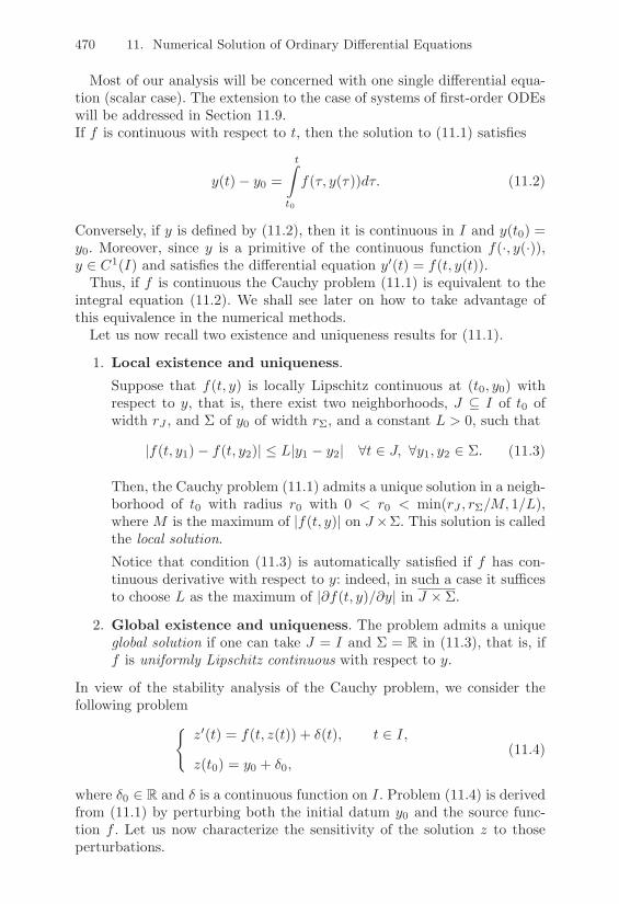
470 11. Numerical Solution of Ordinary Di"erential Equations
Most of our analysis will be concerned with one single di!erential equa-tion (scalar case). The extension to the case of systems of first-order ODEswill be addressed in Section 11.9.If f is continuous with respect to t, then the solution to (11.1) satisfies
y(t)" y0 =t^
t0
f(5, y(5))d5. (11.2)
Conversely, if y is defined by (11.2), then it is continuous in I and y(t0) =y0. Moreover, since y is a primitive of the continuous function f(·, y(·)),y ! C1(I) and satisfies the di!erential equation y*(t) = f(t, y(t)).
Thus, if f is continuous the Cauchy problem (11.1) is equivalent to theintegral equation (11.2). We shall see later on how to take advantage ofthis equivalence in the numerical methods.
Let us now recall two existence and uniqueness results for (11.1).
1. Local existence and uniqueness.Suppose that f(t, y) is locally Lipschitz continuous at (t0, y0) withrespect to y, that is, there exist two neighborhoods, J 7 I of t0 ofwidth rJ , and & of y0 of width r#, and a constant L > 0, such that
|f(t, y1)" f(t, y2)| & L|y1 " y2| #t ! J, #y1, y2 ! &. (11.3)
Then, the Cauchy problem (11.1) admits a unique solution in a neigh-borhood of t0 with radius r0 with 0 < r0 < min(rJ , r#/M, 1/L),where M is the maximum of |f(t, y)| on J%&. This solution is calledthe local solution.Notice that condition (11.3) is automatically satisfied if f has con-tinuous derivative with respect to y: indeed, in such a case it su"cesto choose L as the maximum of |.f(t, y)/.y| in J % &.
2. Global existence and uniqueness. The problem admits a uniqueglobal solution if one can take J = I and & = R in (11.3), that is, iff is uniformly Lipschitz continuous with respect to y.
In view of the stability analysis of the Cauchy problem, we consider thefollowing problem
Bz*(t) = f(t, z(t)) + %(t), t ! I,
z(t0) = y0 + %0,(11.4)
where %0 ! R and % is a continuous function on I. Problem (11.4) is derivedfrom (11.1) by perturbing both the initial datum y0 and the source func-tion f . Let us now characterize the sensitivity of the solution z to thoseperturbations.

11.1 The Cauchy Problem 471
Definition 11.1 ([Hah67], [Ste71] or [PS91]). Let I be a bounded set. TheCauchy problem (11.1) is stable in the sense of Liapunov (or stable) on Iif, for any perturbation (%0, %(t)) satisfying
|%0| < +, |%(t)| < + #t ! I,
with + > 0 su"ciently small to guarantee that the solution to the perturbedproblem (11.4) does exist, then
-C > 0 independent of + such that |y(t)" z(t)| < C+, #t ! I.(11.5)
If I has no upperly bound we say that (11.1) is asymptotically stable if, aswell as being Liapunov stable in any bounded interval I, the following limitalso holds
|y(t)" z(t)|( 0, for t( +,. (11.6)
!The requirement that the Cauchy problem is stable is equivalent to requir-ing that it is well-posed in the sense stated in Chapter 2.
The uniform Lipschitz-continuity of f with respect to y su"ces to ensurethe stability of the Cauchy problem. Indeed, letting w(t) = z(t)" y(t), wehave
w*(t) = f(t, z(t))" f(t, y(t)) + %(t).Therefore,
w(t) = %0 +t^
t0
[f(s, z(s))" f(s, y(s))] ds +t^
t0
%(s)ds, #t ! I.
Thanks to previous assumptions, it follows that
|w(t)| & (1 + |t" t0|) ++ L
t^
t0
|w(s)|ds.
Applying the Gronwall lemma (which we include below for the reader’sease) yields
|w(t)| & (1 + |t" t0|) +eL|t"t0|, #t ! I
and, thus, (11.5) with C = (1 + KI)eLKI where KI = maxt#I |t" t0|.
Lemma 11.1 (Gronwall) Let p be an integrable function nonnegative onthe interval (t0, t0 + T ), and let g and 1 be two continuous functions on[t0, t0 + T ], g being nondecreasing. If 1 satisfies the inequality
1(t) & g(t) +t^
t0
p(5)1(5)d5, #t ! [t0, t0 + T ],

472 11. Numerical Solution of Ordinary Di"erential Equations
then
1(t) & g(t) exp
G
Ht^
t0
p(5)d5
I
J, #t ! [t0, t0 + T ].
For the proof, see, for instance, [QV94], Lemma 1.4.1.
The constant C that appears in (11.5) could be very large and, in general,depends on the upper extreme of the interval I, as in the proof above.For that reason, the property of asymptotic stability is more suitable fordescribing the behavior of the dynamical system (11.1) as t ( +, (see[Arn73]).
As is well-known, only a restricted number of nonlinear ODEs can besolved in closed form (see, for instance, [Arn73]). Moreover, even whenthis is possible, it is not always a straightforward task to find an explicitexpression of the solution; for example, consider the (very simple) equationy* = (y" t)/(y+ t), whose solution is only implicitly defined by the relation(1/2) log(t2 + y2) + tan"1(y/t) = C, where C is a constant depending onthe initial condition.
For this reason we are interested in numerical methods, since these canbe applied to any ODE under the sole condition that it admits a uniquesolution.
11.2 One-Step Numerical Methods
Let us address the numerical approximation of the Cauchy problem (11.1).Fix 0 < T < +, and let I = (t0, t0 + T ) be the integration interval and,correspondingly, for h > 0, let tn = t0 + nh, with n = 0, 1, 2, . . . , Nh, bethe sequence of discretization nodes of I into subintervals In = [tn, tn+1].The width h of such subintervals is called the discretization stepsize. Noticethat Nh is the maximum integer such that tNh & t0 + T . Let uj be theapproximation at node tj of the exact solution y(tj); this solution will behenceforth shortly denoted by yj . Similarly, fj denotes the value f(tj , uj).We obviously set u0 = y0.
Definition 11.2 A numerical method for the approximation of problem(11.1) is called a one-step method if #n ) 0, un+1 depends only on un.Otherwise, the scheme is called a multistep method. !
For now, we focus our attention on one-step methods. Here are some ofthem:

11.3 Analysis of One-Step Methods 473
1. forward Euler method
un+1 = un + hfn; (11.7)
2. backward Euler method
un+1 = un + hfn+1. (11.8)
In both cases, y* is approximated through a finite di!erence: forward andbackward di!erences are used in (11.7) and (11.8), respectively. Both finitedi!erences are first-order approximations of the first derivative of y withrespect to h (see Section 10.10.1).
3. trapezoidal (or Crank-Nicolson) method
un+1 = un +h
2[fn + fn+1] . (11.9)
This method stems from approximating the integral on the right side of(11.2) by the trapezoidal quadrature rule (9.11).
4. Heun method
un+1 = un +h
2[fn + f(tn+1, un + hfn)]. (11.10)
This method can be derived from the trapezoidal method substitutingf(tn+1, un + hf(tn, un)) for f(tn+1, un+1) in (11.9) (i.e., using the forwardEuler method to compute un+1).
In this last case, we notice that the aim is to transform an implicit methodinto an explicit one. Addressing this concern, we recall the following.
Definition 11.3 (explicit and implicit methods) A method is calledexplicit if un+1 can be computed directly in terms of (some of) the previousvalues uk, k & n. A method is said to be implicit if un+1 depends implicitlyon itself through f . !Methods (11.7) and (11.10) are explicit, while (11.8) and (11.9) are implicit.These latter require at each time step to solving a nonlinear problem if fdepends nonlinearly on the second argument.
A remarkable example of one-step methods are the Runge-Kutta meth-ods, which will be analyzed in Section 11.8.
11.3 Analysis of One-Step Methods
Any one-step explicit method for the approximation of (11.1) can be castin the concise form
un+1 = un + h'(tn, un, fn;h), 0 & n & Nh " 1, u0 = y0, (11.11)

474 11. Numerical Solution of Ordinary Di"erential Equations
where '(·, ·, ·; ·) is called an increment function. Letting as usual yn = y(tn),analogously to (11.11) we can write
yn+1 = yn + h'(tn, yn, f(tn, yn);h) + +n+1, 0 & n & Nh " 1, (11.12)
where +n+1 is the residual arising at the point tn+1 when we pretend thatthe exact solution “satisfies” the numerical scheme. Let us write the residualas
+n+1 = h5n+1(h).
The quantity 5n+1(h) is called the local truncation error (LTE) at the nodetn+1. We thus define the global truncation error to be the quantity
5(h) = max0%n%Nh"1
|5n+1(h)|
Notice that 5(h) depends on the solution y of the Cauchy problem (11.1).The forward Euler’s method is a special instance of (11.11), where
'(tn, un, fn;h) = fn,
while to recover Heun’s method we must set
'(tn, un, fn;h) =12
[fn + f(tn + h, un + hfn)] .
A one-step explicit scheme is fully characterized by its increment function'. This function, in all the cases considered thus far, is such that
limh&0
'(tn, yn, f(tn, yn);h) = f(tn, yn), #tn ) t0 (11.13)
Property (11.13), together with the obvious relation yn+1" yn = hy*(tn)+O(h2), #n ) 0, allows one to obtain from (11.12) that lim
h&05n(h) = 0,
0 & n & Nh " 1. In turn, this condition ensures that
limh&0
5(h) = 0
which expresses the consistency of the numerical method (11.11) with theCauchy problem (11.1). In general, a method is said to be consistent if itsLTE is infinitesimal with respect to h. Moreover, a scheme has order p if,#t ! I, the solution y(t) of the Cauchy problem (11.1) fulfills the condition
5(h) = O(hp) for h( 0. (11.14)
Using Taylor expansions, as was done in Section 11.2, it can be proved thatthe forward Euler method has order 1, while the Heun method has order 2(see Exercises 1 and 2).

11.3 Analysis of One-Step Methods 475
11.3.1 The Zero-StabilityLet us formulate a requirement analogous to the one for Liapunov stability(11.5), specifically for the numerical scheme. If (11.5) is satisfied with aconstant C independent of h, we shall say that the numerical problem iszero-stable. Precisely:
Definition 11.4 (zero-stability of one-step methods) The numericalmethod (11.11) for the approximation of problem (11.1) is zero-stable if
-h0 > 0, -C > 0 : #h ! (0, h0], |z(h)n " u(h)
n | & C+, 0 & n & Nh, (11.15)
where z(h)n , u(h)
n are respectively the solutions of the problems)+
,z(h)n+1 = z(h)
n + hV'(tn, z
(h)n , f(tn, z
(h)n );h) + %n+1
W,
z0 = y0 + %0,(11.16)
)+
,u(h)n+1 = u(h)
n + h'(tn, u(h)n , f(tn, u
(h)n );h),
u0 = y0,(11.17)
for 0 & n & Nh " 1, under the assumption that |%k| & +, 0 & k & Nh. !
Zero-stability thus requires that, in a bounded interval, (11.15) holds forany value h & h0. This property deals, in particular, with the behaviorof the numerical method in the limit case h ( 0 and this justifies thename of zero-stability. This latter is therefore a distinguishing property ofthe numerical method itself, not of the Cauchy problem (which, indeed,is stable due to the uniform Lipschitz continuity of f). Property (11.15)ensures that the numerical method has a weak sensitivity with respect tosmall changes in the data and is thus stable in the sense of the generaldefinition given in Chapter 2.
Remark 11.1 The constant C in (11.15) is independent of h (and thusof Nh), but it can depend on the width T of the integration interval I.Actually, (11.15) does not exclude a priori the constant C from being anunbounded function of T . !
The request that a numerical method be stable arises, before anything else,from the need of keeping under control the (unavoidable) errors introducedby the finite arithmetic of the computer. Indeed, if the numerical methodwere not zero-stable, the rounding errors made on y0 as well as in the pro-cess of computing f(tn, un) would make the computed solution completelyuseless.

476 11. Numerical Solution of Ordinary Di"erential Equations
Theorem 11.1 (Zero-stability) Consider the explicit one-step method(11.11) for the numerical solution of the Cauchy problem (11.1). Assumethat the increment function ' is Lipschitz continuous with respect to thesecond argument, with constant % independent of h and of the nodes tj ![t0, t0 + T ], that is
-h0 > 0, -% > 0 : #h ! (0, h0]
|'(tn, u(h)n , f(tn, u
(h)n );h)" '(tn, z
(h)n , f(tn, z
(h)n );h)|
& %|u(h)n " z(h)
n |, 0 & n & Nh.
(11.18)
Then, method (11.11) is zero-stable.
Proof. Setting w(h)j = z(h)
j %u(h)j , by subtracting (11.17) from (11.16) we obtain,
for j = 0, . . . , Nh % 1,
w(h)j+1 = w(h)
j + hV%(tj , z(h)
j , f(tj , z(h)j );h)% %(tj , u(h)
j , f(tj , u(h)j );h)
W+ h!j+1.
Summing over j gives, for n = 1, . . . , Nh,
w(h)n = w(h)
0
+hn%1(
j=0
!j+1 + hn%1(
j=0
K%(tj , z(h)
j , f(tj , z(h)j );h)% %(tj , u(h)
j , f(tj , u(h)j );h)
L,
so that, by (11.18)
|w(h)n | " |w0| + h
n%1(
j=0
|!j+1| + h&n%1(
j=0
|w(h)j |, 1 " n " Nh. (11.19)
Applying the discrete Gronwall lemma, given below, we obtain
|w(h)n | " (1 + hn) &enh", 1 " n " Nh.
Then (11.15) follows from noticing that hn " T and setting C = (1 + T ) e"T . !
Notice that zero-stability implies the boundedness of the solution when fis linear with respect to the second argument.
Lemma 11.2 (discrete Gronwall) Let kn be a nonnegative sequence and1n a sequence such that
)**+
**,
10 & g0
1n & g0 +n"1(
s=0
ps +n"1(
s=0
ks4s, n ) 1.
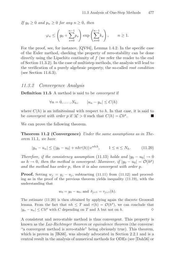
11.3 Analysis of One-Step Methods 477
If g0 ) 0 and pn ) 0 for any n ) 0, then
1n &6
g0 +n"1(
s=0
ps
7
exp
6n"1(
s=0
ks
7
, n ) 1.
For the proof, see, for instance, [QV94], Lemma 1.4.2. In the specific caseof the Euler method, checking the property of zero-stability can be donedirectly using the Lipschitz continuity of f (we refer the reader to the endof Section 11.3.2). In the case of multistep methods, the analysis will lead tothe verification of a purely algebraic property, the so-called root condition(see Section 11.6.3).
11.3.2 Convergence AnalysisDefinition 11.5 A method is said to be convergent if
#n = 0, . . . , Nh, |un " yn| & C(h)
where C(h) is an infinitesimal with respect to h. In that case, it is said tobe convergent with order p if -C > 0 such that C(h) = Chp. !
We can prove the following theorem.
Theorem 11.2 (Convergence) Under the same assumptions as in The-orem 11.1, we have
|yn " un| & (|y0 " u0| + nh5(h)) enh$, 1 & n & Nh. (11.20)
Therefore, if the consistency assumption (11.13) holds and |y0 " u0| ( 0as h ( 0, then the method is convergent. Moreover, if |y0 " u0| = O(hp)and the method has order p, then it is also convergent with order p.
Proof. Setting wj = yj % uj , subtracting (11.11) from (11.12) and proceed-ing as in the proof of the previous theorem yields inequality (11.19), with theunderstanding that
w0 = y0 % u0, and !j+1 = 4j+1(h).
The estimate (11.20) is then obtained by applying again the discrete Gronwalllemma. From the fact that nh " T and 4(h) = O(hp), we can conclude that|yn % un| " Chp with C depending on T and & but not on h. !
A consistent and zero-stable method is thus convergent. This property isknown as the Lax-Richtmyer theorem or equivalence theorem (the converse:“a convergent method is zero-stable” being obviously true). This theorem,which is proven in [IK66], was already advocated in Section 2.2.1 and is acentral result in the analysis of numerical methods for ODEs (see [Dah56] or

478 11. Numerical Solution of Ordinary Di"erential Equations
[Hen62] for linear multistep methods, [But66], [MNS74] for a wider classesof methods). It will be considered again in Section 11.5 for the analysis ofmultistep methods.
We carry out in detail the convergence analysis in the case of the forwardEuler method, without resorting to the discrete Gronwall lemma. In thefirst part of the proof we assume that any operation is performed in exactarithmetic and that u0 = y0.
Denote by en+1 = yn+1 " un+1 the error at node tn+1 with n = 0, 1, . . .and notice that
en+1 = (yn+1 " u,n+1) + (u,
n+1 " un+1), (11.21)
where u,n+1 = yn + hf(tn, yn) is the solution obtained after one step of
the forward Euler method starting from the initial datum yn (see Figure11.1). The first addendum in (11.21) accounts for the consistency error, thesecond one for the cumulation of these errors. Then
yn+1 " u,n+1 = h5n+1(h), u,
n+1 " un+1 = en + h [f(tn, yn)" f(tn, un)] .
y(x)
yn
un
tn tn+1
un+1
u,n+1
yn+1
h5n+1en+1
FIGURE 11.1. Geometrical interpretation of the local and global truncation er-rors at node tn+1 for the forward Euler method
As a consequence,
|en+1| & h|5n+1(h)| + |en| + h|f(tn, yn)" f(tn, un)| & h5(h) + (1 + hL)|en|,
L being the Lipschitz constant of f . By recursion on n, we find
|en+1| & [1 + (1 + hL) + . . . + (1 + hL)n]h5(h)
=(1 + hL)n+1 " 1
L5(h) & eL(tn+1"t0) " 1
L5(h).

11.3 Analysis of One-Step Methods 479
The last inequality follows from noticing that 1+hL & ehL and (n+1)h =tn+1 " t0.
On the other hand, if y ! C2(I), the LTE for the forward Euler methodis (see Section 10.10.1)
5n+1(h) =h
2y**(*), * ! (tn, tn+1),
and thus, 5(h) & (M/2)h, where M = max0#I |y**(*)|. In conclusion,
|en+1| &eL(tn+1"t0) " 1
L
M
2h, #n ) 0, (11.22)
from which it follows that the global error tends to zero with the sameorder as the local truncation error.
If also the rounding errors are accounted for, we can assume that thesolution un+1, actually computed by the forward Euler method at timetn+1, is such that
u0 = y0 + 80, un+1 = un + hf(tn, un) + 8n+1, (11.23)
having denoted the rounding error by 8j , for j ) 0.Problem (11.23) is an instance of (11.16), provided that we identify 8n+1
and un with h%n+1 and z(h)n in (11.16), respectively. Combining Theorems
11.1 and 11.2 we get, instead of (11.22), the following error estimate
|yn+1 " un+1| & eL(tn+1"t0)-|80| +
1L
4M
2h +
8
h
5.,
where 8 = max1%j%n+1 |8j |. The presence of rounding errors does not allow,therefore, to conclude that as h ( 0, the error goes to zero. Actually,there exists an optimal (non null) value of h, hopt, for which the error isminimized. For h < hopt, the rounding error dominates the truncation errorand the global error increases.
11.3.3 The Absolute StabilityThe property of absolute stability is in some way specular to zero-stability,as far as the roles played by h and I are concerned. Heuristically, we say thata numerical method is absolutely stable if, for h fixed, un remains boundedas tn ( +,. This property, thus, deals with the asymptotic behavior ofun, as opposed to a zero-stable method for which, for a fixed integrationinterval, un remains bounded as h( 0.For a precise definition, consider the linear Cauchy problem (that from nowon, we shall refer to as the test problem)
By*(t) = $y(t), t > 0,
y(0) = 1,(11.24)

480 11. Numerical Solution of Ordinary Di"erential Equations
with $ ! C, whose solution is y(t) = e#t. Notice that limt&+$
|y(t)| = 0 if
Re($) < 0.
Definition 11.6 A numerical method for approximating (11.24) is abso-lutely stable if
|un| "( 0 as tn "( +,. (11.25)
Let h be the discretization stepsize. The numerical solution un of (11.24)obviously depends on h and $. The region of absolute stability of the nu-merical method is the subset of the complex plane
A = {z = h$ ! C : (11.25) is satisfied } . (11.26)
Thus, A is the set of the values of the product h$ for which the numericalmethod furnishes solutions that decay to zero as tn tends to infinity. !
Let us check whether the one-step methods introduced previously are ab-solutely stable.
1. Forward Euler method: applying (11.7) to problem (11.24) yields un+1 =un + h$un for n ) 0, with u0 = 1. Proceeding recursively on n we get
un = (1 + h$)n, n ) 0.
Therefore, condition (11.25) is satisfied i! |1 + h$| < 1, that is, if h$ lieswithin the unit circle with center at ("1, 0) (see Figure 11.3). This amountsto requiring that
h$ ! C" and 0 < h < "2Re($)|$|2 (11.27)
where
C" = {z ! C : Re(z) < 0} .
Example 11.1 For the Cauchy problem y((x) = %5y(x) for x > 0 and y(0) = 1,condition (11.27) implies 0 < h < 2/5. Figure 11.2 (left) shows the behavior ofthe computed solution for two values of h which do not fulfill this condition, whileon the right we show the solutions for two values of h that do. Notice that in thissecond case the oscillations, if present, damp out as t grows. •
2. Backward Euler method: proceeding as before, we get this time
un =1
(1" h$)n, n ) 0.
The absolute stability property (11.25) is satisfied for any value of h$ thatdoes not belong to the unit circle of center (1, 0) (see Figure 11.3, right).

11.3 Analysis of One-Step Methods 481
0 1 2 3 4 5 6 7 8!3
!2
!1
0
1
2
3
0 1 2 3 4 5 6 7 8!1
!0.8
!0.6
!0.4
!0.2
0
0.2
0.4
0.6
0.8
1
FIGURE 11.2. Left: computed solutions for h = 0.41 > 2/5 (dashed line) andh = 2/5 (solid line). Notice how, in the limiting case h = 2/5, the oscillationsremain unmodified as t grows. Right: two solutions are reported for h = 0.39(solid line) and h = 0.15 (dashed line)
Example 11.2 The numerical solution given by the backward Euler method inthe case of Example 11.1 does not exhibit any oscillation for any value of h. Onthe other hand, the same method, if applied to the problem y((t) = 5y(t) for t > 0and with y(0) = 1, computes a solution that decays anyway to zero as t,# ifh > 2/5, despite the fact that the exact solution of the Cauchy problem tends toinfinity. •
3. Trapezoidal (or Crank-Nicolson) method: we get
un =-4
1 +12$h
5/
41" 1
2$h
5.n
, n ) 0,
hence (11.25) is fulfilled for any h$ ! C".
4. Heun’s method: applying (11.10) to problem (11.24) and proceedingby recursion on n, we obtain
un =-1 + h$+
(h$)2
2
.n
, n ) 0.
As shown in Figure 11.3 the region of absolute stability of Heun’s methodis larger than the corresponding one of Euler’s method. However, its re-striction to the real axis is the same.We say that a method is A-stable if A 8 C" = C", i.e., if for Re($) < 0,condition (11.25) is satisfied for all values of h.
The backward Euler and Crank-Nicolson methods are A-stable, whilethe forward Euler and Heun methods are conditionally stable.
Remark 11.2 Notice that the implicit one-step methods examined so farare unconditionally absolutely stable, while explicit schemes are condition-

482 11. Numerical Solution of Ordinary Di"erential Equations
FE
H
Re
BE
"1 1
Im
1.75
"1.75
FIGURE 11.3. Regions of absolute stability for the forward (FE) and backwardEuler (BE) methods and for Heun’s method (H). Notice that the region of abso-lute stability of the BE method lies outside the unit circle of center (1, 0) (shadedarea)
ally absolutely stable. This is, however, not a general rule: in fact, there ex-ist implicit unstable or only conditionally stable schemes. On the contrary,there are no explicit unconditionally absolutely stable schemes [Wid67]. !
11.4 Di"erence Equations
For any integer k ) 1, an equation of the form
un+k + "k"1un+k"1 + . . . + "0un = 1n+k, n = 0, 1, . . . (11.28)
is called a linear di!erence equation of order k. The coe"cients "0 '= 0,"1, . . . ,"k"1 may or may not depend on n. If, for any n, the right side1n+k is equal to zero, the equation is said homogeneous, while if the "*
jsare independent of n it is called linear di!erence equation with constantcoe"cients.Di!erence equations arise for instance in the discretization of ordinary dif-ferential equations. Regarding this, we notice that all the numerical meth-ods examined so far end up with equations like (11.28). More generally,equations like (11.28) are encountered when quantities are defined throughlinear recursive relations. Another relevant application is concerned withthe discretization of boundary value problems (see Chapter 12). For fur-ther details on the subject, we refer to Chapters 2 and 5 of [BO78] and toChapter 6 of [Gau97].

11.4 Di"erence Equations 483
Any sequence {un, n = 0, 1, . . . } of values that satisfy (11.28) is calleda solution to the equation (11.28). Given k initial values u0, . . . , uk"1, itis always possible to construct a solution of (11.28) by computing (sequen-tially)
un+k = [1n+k " ("k"1un+k"1 + . . . + "0un)], n = 0, 1, . . .
However, our interest is to find an expression of the solution un+k whichdepends only on the coe"cients and on the initial values.
We start by considering the homogeneous case with constant coe"cients,
un+k + "k"1un+k"1 + . . . + "0un = 0, n = 0, 1, . . . (11.29)
and associate with (11.29) the characteristic polynomial $ ! Pk defined as
$(r) = rk + "k"1rk"1 + . . . + "1r + "0. (11.30)
Denoting its roots by rj , j = 0, . . . , k " 1, any sequence of the form/rnj , n = 0, 1, . . .
0, for j = 0, . . . , k " 1 (11.31)
is a solution of (11.29), since
rn+kj + "k"1r
n+k"1j + . . . + "0rnj
= rnj8rkj + "k"1r
k"1j + . . . + "0
9= rnj $(rj) = 0.
We say that the k sequences defined in (11.31) are the fundamental solutionsof the homogeneous equation (11.29). Any sequence of the form
un = '0rn0 + '1r
n1 + . . . + 'k"1r
nk"1, n = 0, 1, . . . (11.32)
is still a solution to (11.29), since it is a linear equation.The coe"cients '0, . . . , 'k"1 can be determined by imposing the k initialconditions u0, . . . , uk"1. Moreover, it can be proved that if all the rootsof $ are simple, then all the solutions of (11.29) can be cast in the form(11.32).
This last statement no longer holds if there are roots of $ with multi-plicity greater than 1. If, for a certain j, the root rj has multiplicity m ) 2,in order to obtain a system of fundamental solutions that generate all thesolutions of (11.29), it su"ces to replace the corresponding fundamentalsolution
/rnj , n = 0, 1, . . .
0with the m sequences
/rnj , n = 0, 1, . . .
0,
/nrnj , n = 0, 1, . . .
0, . . . ,
/nm"1rnj , n = 0, 1, . . .
0.
More generally, assuming that r0, . . . , rk% are distinct roots of $, with mul-tiplicities equal to m0, . . . ,mk% , respectively, we can write the solution of(11.29) as
un =k%(
j=0
6mj"1(
s=0
'sjns
7
rnj , n = 0, 1, . . . . (11.33)

484 11. Numerical Solution of Ordinary Di"erential Equations
Notice that even in presence of complex conjugate roots one can still obtaina real solution (see Exercise 3).
Example 11.3 For the di"erence equation un+2%un = 0, we have ((r) = r2%1,then r0 = %1 and r1 = 1, therefore the solution is given by un = ,00(%1)n + ,01.In particular, enforcing the initial conditions u0 and u1 gives ,00 = (u0 % u1)/2,,01 = (u0 + u1)/2. •
Example 11.4 For the di"erence equation un+3 % 2un+2 % 7un+1 % 4un = 0,((r) = r3 % 2r2 % 7r % 4. Its roots are r0 = %1 (with multiplicity 2), r1 = 4 andthe solution is un = (,00 + n,10)(%1)n + ,014n. Enforcing the initial conditionswe can compute the unknown coe!cients as the solution of the following linearsystem
)+
,
,00 + ,01 = u0,%,00 % ,10 + 4,01 = u1,,00 + 2,10 + 16,01 = u2
that yields ,00 = (24u0 % 2u1 % u2)/25, ,10 = (u2 % 3u1 % 4u0)/5 and ,01 =(2u1 + u0 + u2)/25. •
The expression (11.33) is of little practical use since it does not outlinethe dependence of un on the k initial conditions. A more convenient rep-resentation is obtained by introducing a new set
R6(n)j , n = 0, 1, . . .
Sof
fundamental solutions that satisfy
6(i)j = %ij , i, j = 0, 1, . . . , k " 1. (11.34)
Then, the solution of (11.29) subject to the initial conditions u0, . . . , uk"1is given by
un =k"1(
j=0
uj6(n)j , n = 0, 1, . . . . (11.35)
The new fundamental solutionsR6(n)j , n = 0, 1, . . .
Scan be represented in
terms of those in (11.31) as follows
6(n)j =
k"1(
m=0
#j,mrnm for j = 0, . . . , k " 1, n = 0, 1, . . . (11.36)
By requiring (11.34), we obtain the k linear systems
k"1(
m=0
#j,mrim = %ij , i, j = 0, . . . , k " 1,
whose matrix form is
Rbj = ej , j = 0, . . . , k " 1. (11.37)

11.4 Di"erence Equations 485
Here ej denotes the unit vector of Rk, R = (rim) = (rim) and bj =(#j,0, . . . ,#j,k"1)T . If all r*js are simple roots of $, the matrix R is nonsin-gular (see Exercise 5).
The general case where $ has k*+1 distinct roots r0, . . . , rk% with multi-plicities m0, . . . ,mk% respectively, can be dealt with by replacing in (11.36)/rnj , n = 0, 1, . . .
0with
/rnj n
s, n = 0, 1, . . .0, where j = 0, . . . , k* and
s = 0, . . . ,mj " 1.
Example 11.5 We consider again the di"erence equation of Example 11.4. Herewe have {rn0 , nrn0 , rn1 , n = 0, 1, . . . } so that the matrix R becomes
R =
"
$r00 0 r0
2r10 r1
0 r12
r20 2r2
0 r22
%
' =
"
$1 0 1
%1 %1 41 2 16
%
' .
Solving the three systems (11.37) yields
5(n)0 =
2425
(%1)n % 45n(%1)n +
125
4n,
5(n)1 = % 2
25(%1)n % 3
5n(%1)n +
225
4n,
5(n)2 = % 1
25(%1)n +
15n(%1)n +
125
4n,
from which it can be checked that the solution un =!2
j=0 uj5(n)j coincides with
the one already found in Example 11.4. •
Now we return to the case of nonconstant coe"cients and consider thefollowing homogeneous equation
un+k +k(
j=1
"k"j(n)un+k"j = 0, n = 0, 1, . . . . (11.38)
The goal is to transform it into an ODE by means of a function F , calledthe generating function of the equation (11.38). F depends on the realvariable t and is derived as follows. We require that the n-th coe"cientof the Taylor series of F around t = 0 can be written as 'nun, for someunknown constant 'n, so that
F (t) =$(
n=0
'nuntn. (11.39)
The coe"cients {'n} are unknown and must be determined in such a waythat
k(
j=0
cjF(k"j)(t) =
$(
n=0
"
$un+k +k(
j=1
"k"j(n)un+k"j
%
' tn, (11.40)
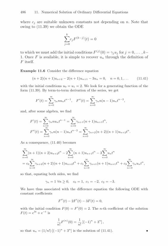
486 11. Numerical Solution of Ordinary Di"erential Equations
where cj are suitable unknown constants not depending on n. Note thatowing to (11.39) we obtain the ODE
k(
j=0
cjF(k"j)(t) = 0
to which we must add the initial conditions F (j)(0) = 'juj for j = 0, . . . , k"1. Once F is available, it is simple to recover un through the definition ofF itself.
Example 11.6 Consider the di"erence equation
(n + 2)(n + 1)un+2 % 2(n + 1)un+1 % 3un = 0, n = 0, 1, . . . (11.41)
with the initial conditions u0 = u1 = 2. We look for a generating function of theform (11.39). By term-to-term derivation of the series, we get
F ((t) =!(
n=0
,nnuntn%1, F (((t) =
!(
n=0
,nn(n% 1)untn%2,
and, after some algebra, we find
F ((t) =!(
n=0
,nnuntn%1 =
!(
n=0
,n+1(n + 1)un+1tn,
F (((t) =!(
n=0
,nn(n% 1)untn%2 =
!(
n=0
,n+2(n + 2)(n + 1)un+2tn.
As a consequence, (11.40) becomes
!(
n=0
(n + 1)(n + 2)un+2tn % 2
!(
n=0
(n + 1)un+1tn % 3
!(
n=0
untn
= c0
!(
n=0
,n+2(n + 2)(n + 1)un+2tn + c1
!(
n=0
,n+1(n + 1)un+1tn + c2
!(
n=0
,nuntn,
so that, equating both sides, we find
,n = 1 )n ! 0, c0 = 1, c1 = %2, c2 = %3.
We have thus associated with the di"erence equation the following ODE withconstant coe!cients
F (((t)% 2F ((t)% 3F (t) = 0,
with the initial condition F (0) = F ((0) = 2. The n-th coe!cient of the solutionF (t) = e3t + e%t is
1n!
F (n)(0) =1n!
[(%1)n + 3n] ,
so that un = (1/n!) [(%1)n + 3n] is the solution of (11.41). •

11.5 Multistep Methods 487
The nonhomogeneous case (11.28) can be tackled by searching for solutionsof the form
un = u(0)n + u(1)
n ,
where u(0)n is the solution of the associated homogeneous equation and u(1)
n
is a particular solution of the nonhomogeneous equation. Once the solutionof the homogeneous equation is available, a general technique to obtainthe solution of the nonhomogeneous equation is based on the method ofvariation of parameters, combined with a reduction of the order of thedi!erence equation (see [BO78]).
In the special case of di!erence equations with constant coe"cients, with1n of the form cnQ(n), where c is a constant and Q is a polynomial of degreep with respect to the variable n, a possible approach is that of undeterminedcoe"cients, where one looks for a particular solution that depends on someundetermined constants and has a known form for some classes of rightsides 1n. It su"ces to look for a particular solution of the form
u(1)n = cn(bpnp + bp"1n
p"1 + . . . + b0),
where bp, . . . , b0 are constants to be determined in such a way that u(1)n is
actually a solution of (11.28).
Example 11.7 Consider the di"erence equation un+3%un+2+un+1%un = 2nn2.The particular solution is of the form un = 2n(b2n2 + b1n+ b0). Substituting thissolution into the equation, we find 5b2n2+(36b2+5b1)n+(58b2+18b1+5b0) = n2,from which, recalling the principle of identity for polynomials, one gets b2 = 1/5,b1 = %36/25 and b0 = 358/125. •
Analogous to the homogeneous case, it is possible to express the solutionof (11.28) as
un =k"1(
j=0
uj6(n)j +
n(
l=k
1l6(n"l+k"1)k"1 , n = 0, 1, . . . (11.42)
where we define 6(i)k"1 ? 0 for all i < 0 and 1j ? 0 for all j < k.
11.5 Multistep Methods
Let us now introduce some examples of multistep methods (shortly, MS).
Definition 11.7 (q-steps methods) A q-step method (q ) 1) is onewhich, #n ) q " 1, un+1 depends on un+1"q, but not on the values uk
with k < n + 1" q. !

488 11. Numerical Solution of Ordinary Di"erential Equations
A well-known two-step explicit method can be obtained by using thecentered finite di!erence (10.61) to approximate the first order derivativein (11.1). This yields the midpoint method
un+1 = un"1 + 2hfn, n ) 1 (11.43)
where u0 = y0, u1 is to be determined and fk denotes the value f(tk, uk).An example of an implicit two-step scheme is the Simpson method, ob-
tained from (11.2) with t0 = tn"1 and t = tn+1 and by using the Cavalieri-Simpson quadrature rule to approximate the integral of f
un+1 = un"1 +h
3[fn"1 + 4fn + fn+1], n ) 1 (11.44)
where u0 = y0, and u1 is to be determined.From these examples, it is clear that a multistep method requires q initial
values u0, . . . , uq"1 for “taking o!”. Since the Cauchy problem providesonly one datum (u0), one way to assign the remaining values consists ofresorting to explicit one-step methods of high order. An example is given byHeun’s method (11.10), other examples are provided by the Runge-Kuttamethods, which will be introduced in Section 11.8.
In this section we deal with linear multistep methods
un+1 =p(
j=0
ajun"j + hp(
j=0
bjfn"j + hb"1fn+1, n = p, p + 1, . . . (11.45)
which are p + 1-step methods, p ) 0. For p = 0, we recover one-stepmethods.
The coe"cients aj , bj are real and fully identify the scheme; they aresuch that ap '= 0 or bp '= 0. If b"1 '= 0 the scheme is implicit, otherwise itis explicit.
We can reformulate (11.45) as follows
p+1(
s=0
"sun+s = hp+1(
s=0
#sf(tn+s, un+s), n = 0, 1, . . . , Nh " (p + 1) (11.46)
having set "p+1 = 1, "s = "ap"s for s = 0, . . . , p and #s = bp"s fors = 0, . . . , p+1. Relation (11.46) is a special instance of the linear di!erenceequation (11.28), where we set k = p+1 and 1n+j = h#jf(tn+j , un+j), forj = 0, . . . , p + 1.Also for MS methods we can characterize consistency in terms of the localtruncation error, according to the following definition.
Definition 11.8 The local truncation error (LTE) 5n+1(h) introduced bythe multistep method (11.45) at tn+1 (for n ) p) is defined through the

11.5 Multistep Methods 489
following relation
h5n+1(h) = yn+1 "
"
$p(
j=0
ajyn"j + hp(
j="1
bjy*n"j
%
' , n ) p, (11.47)
where yn"j = y(tn"j) and y*n"j = y*(tn"j) for j = "1, . . . , p. !
Analogous to one-step methods, the quantity h5n+1(h) is the residual gen-erated at tn+1 if we pretend that the exact solution “satisfies” the numericalscheme. Letting 5(h) = max
n|5n(h)|, we have the following definition.
Definition 11.9 (Consistency) The multistep method (11.45) is consis-tent if 5(h) ( 0 as h( 0. Moreover, if 5(h) = O(hq), for some q ) 1, thenthe method is said to have order q. !
A more precise characterization of the LTE can be given by introducing thefollowing linear operator L associated with the linear MS method (11.45)
L[w(t);h] = w(t + h)"p(
j=0
ajw(t" jh)" hp(
j="1
bjw*(t" jh), (11.48)
where w ! C1(I) is an arbitrary function. Notice that the LTE is exactlyL[y(tn);h]. If we assume that w is su"ciently smooth and expand w(t"jh)and w*(t" jh) about t" ph, we obtain
L[w(t);h] = C0w(t" ph) + C1hw(1)(t" ph) + . . . + Ckh
kw(k)(t" ph) + . . .
Consequently, if the MS method has order q and y ! Cq+1(I), we obtain
5n+1(h) = Cq+1hq+1y(q+1)(tn"p) + O(hq+2).
The term Cq+1hq+1y(q+1)(tn"p) is the so-called principal local truncationerror (PLTE) while Cq+1 is the error constant. The PLTE is widely em-ployed in devising adaptive strategies for MS methods (see [Lam91], Chap-ter 3).
Program 92 provides an implementation of the multistep method in theform (11.45) for the solution of a Cauchy problem on the interval (t0, T ).The input parameters are: the column vector a containing the p + 1 co-e"cients ai; the column vector b containing the p + 2 coe"cients bi; thediscretization stepsize h; the vector of initial data u0 at the correspondingtime instants t0; the macros fun and dfun containing the functions f and.f/.y. If the MS method is implicit, a tolerance tol and a maximum num-ber of admissible iterations itmax must be provided. These two parametersmonitor the convergence of Newton’s method that is employed to solve the

490 11. Numerical Solution of Ordinary Di"erential Equations
nonlinear equation (11.45) associated with the MS method. In output thecode returns the vectors u and t containing the computed solution at thetime instants t.
Program 92 - multistep : Linear multistep methods
function [t,u] = multistep (a,b,tf,t0,u0,h,fun,dfun,tol,itmax)y = u0; t = t0; f = eval (fun); p = length(a) - 1; u = u0;nt = fix((tf - t0 (1) )/h);for k = 1:nt
lu=length(u);G = a’ *u (lu:-1:lu-p)+ h * b(2:p+2)’ * f(lu:-1:lu-p);lt = length(t0); t0 = [t0; t0(lt)+h]; unew = u (lu);t = t0 (lt+1); err = tol + 1; it = 0;while (err > tol) & (it <= itmax)y = unew; den = 1 - h * b (1) * eval(dfun);fnew = eval (fun);if den == 0
it = itmax + 1;else
it = it + 1;unew = unew - (unew - G - h * b (1) * fnew)/den;err = abs (unew - y);
endendu = [u; unew]; f = [f; fnew];
endt = t0;
In the forthcoming sections we examine some families of multistep methods.
11.5.1 Adams MethodsThese methods are derived from the integral form (11.2) through an ap-proximate evaluation of the integral of f between tn and tn+1. We supposethat the discretization nodes are equally spaced, i.e., tj = t0 + jh, withh > 0 and j ) 1, and then we integrate, instead of f , its interpolatingpolynomial on p+ 1 distinct nodes. The resulting schemes are thus consis-tent by construction and have the following form
un+1 = un + hp(
j="1
bjfn"j , n ) p. (11.49)
The interpolation nodes can be either:
1. tn, tn"1, . . . , tn"p (in this case b"1 = 0 and the resulting method isexplicit);or
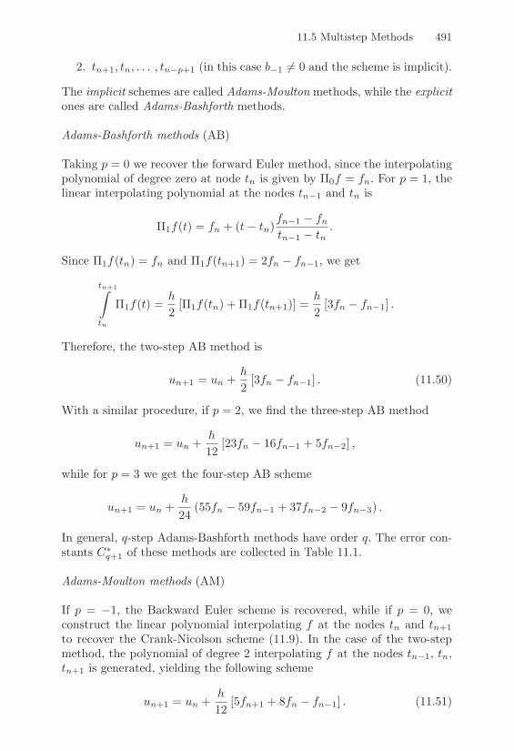
11.5 Multistep Methods 491
2. tn+1, tn, . . . , tn"p+1 (in this case b"1 '= 0 and the scheme is implicit).
The implicit schemes are called Adams-Moulton methods, while the explicitones are called Adams-Bashforth methods.
Adams-Bashforth methods (AB)
Taking p = 0 we recover the forward Euler method, since the interpolatingpolynomial of degree zero at node tn is given by $0f = fn. For p = 1, thelinear interpolating polynomial at the nodes tn"1 and tn is
$1f(t) = fn + (t" tn)fn"1 " fntn"1 " tn
.
Since $1f(tn) = fn and $1f(tn+1) = 2fn " fn"1, we get
tn+1^
tn
$1f(t) =h
2[$1f(tn) +$1f(tn+1)] =
h
2[3fn " fn"1] .
Therefore, the two-step AB method is
un+1 = un +h
2[3fn " fn"1] . (11.50)
With a similar procedure, if p = 2, we find the three-step AB method
un+1 = un +h
12[23fn " 16fn"1 + 5fn"2] ,
while for p = 3 we get the four-step AB scheme
un+1 = un +h
24(55fn " 59fn"1 + 37fn"2 " 9fn"3) .
In general, q-step Adams-Bashforth methods have order q. The error con-stants C,
q+1 of these methods are collected in Table 11.1.
Adams-Moulton methods (AM)
If p = "1, the Backward Euler scheme is recovered, while if p = 0, weconstruct the linear polynomial interpolating f at the nodes tn and tn+1to recover the Crank-Nicolson scheme (11.9). In the case of the two-stepmethod, the polynomial of degree 2 interpolating f at the nodes tn"1, tn,tn+1 is generated, yielding the following scheme
un+1 = un +h
12[5fn+1 + 8fn " fn"1] . (11.51)

492 11. Numerical Solution of Ordinary Di"erential Equations
The methods corresponding to p = 3 and 4 are respectively given by
un+1 = un +h
24(9fn+1 + 19fn " 5fn"1 + fn"2)
un+1 = un +h
720(251fn+1 + 646fn " 264fn"1 + 106fn"2 " 19fn"3) .
The q-step Adams-Moulton methods have order q + 1 and their error con-stants Cq+1 are summarized in Table 11.1.
q C,q+1 Cq+1 q C,
q+1 Cq+1
1 12 " 1
2 3 38 " 1
24
2 512 " 1
12 4 251720 " 19
720
TABLE 11.1. Error constants for Adams-Bashforth methods (having order q) andAdams-Moulton methods (having order q + 1)
11.5.2 BDF MethodsThe so-called backward di!erentiation formulae (henceforth denoted byBDF) are implicit MS methods derived from a complementary approachto the one followed for the Adams methods. In fact, for the Adams meth-ods we have resorted to numerical integration for the source function f ,whereas in BDF methods we directly approximate the value of the firstderivative of y at node tn+1 through the first derivative of the polynomialinterpolating y at the p + 1 nodes tn+1, tn, . . . , tn"p+1.
By doing so, we get schemes of the form
un+1 =p(
j=0
ajun"j + hb"1fn+1
with b"1 '= 0. Method (11.8) represents the most elementary example,corresponding to the coe"cients a0 = 1 and b"1 = 1.
We summarize in Table 11.2 the coe"cients of BDF methods that arezero-stable. In fact, we shall see in Section 11.6.3 that only for p & 5 areBDF methods zero-stable (see [Cry73]).
11.6 Analysis of Multistep Methods
Analogous to what has been done for one-step methods, in this sectionwe provide algebraic conditions that ensure consistency and stability ofmultistep methods.
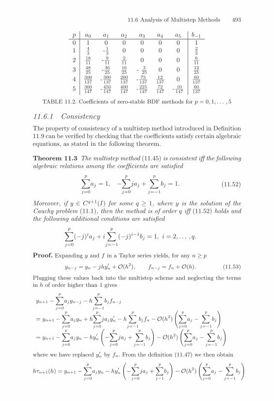
11.6 Analysis of Multistep Methods 493
p a0 a1 a2 a3 a4 a5 b"10 1 0 0 0 0 0 11 4
3 - 13 0 0 0 0 2
3
2 1811 - 9
11211 0 0 0 6
11
3 4825 - 36
251625 - 3
25 0 0 1225
4 300137 - 300
137200137 - 75
13712137 0 60
137
5 360147 - 450
147400147 - 225
14772147 - 10
14760137
TABLE 11.2. Coe!cients of zero-stable BDF methods for p = 0, 1, . . . , 5
11.6.1 ConsistencyThe property of consistency of a multistep method introduced in Definition11.9 can be verified by checking that the coe"cients satisfy certain algebraicequations, as stated in the following theorem.
Theorem 11.3 The multistep method (11.45) is consistent i! the followingalgebraic relations among the coe"cients are satisfied
p(
j=0
aj = 1, "p(
j=0
jaj +p(
j="1
bj = 1. (11.52)
Moreover, if y ! Cq+1(I) for some q ) 1, where y is the solution of theCauchy problem (11.1), then the method is of order q i! (11.52) holds andthe following additional conditions are satisfied
p(
j=0
("j)iaj + ip(
j="1
("j)i"1bj = 1, i = 2, . . . , q.
Proof. Expanding y and f in a Taylor series yields, for any n ! p
yn%j = yn % jhy(n + O(h2), fn%j = fn + O(h). (11.53)
Plugging these values back into the multistep scheme and neglecting the termsin h of order higher than 1 gives
yn+1 %p(
j=0
ajyn%j % hp(
j=%1
bjfn%j
= yn+1 %p(
j=0
ajyn + hp(
j=0
jajy(n % h
p(
j=%1
bjfn %O(h2)
6p(
j=0
aj %p(
j=%1
bj
7
= yn+1 %p(
j=0
ajyn % hy(n
6
%p(
j=0
jaj +p(
j=%1
bj
7
%O(h2)
6p(
j=0
aj %p(
j=%1
bj
7
where we have replaced y(n by fn. From the definition (11.47) we then obtain
h4n+1(h) = yn+1 %p(
j=0
ajyn % hy(n
6
%p(
j=0
jaj +p(
j%1
bj
7
%O(h2)
6p(
j=0
aj %p(
j=%1
bj
7
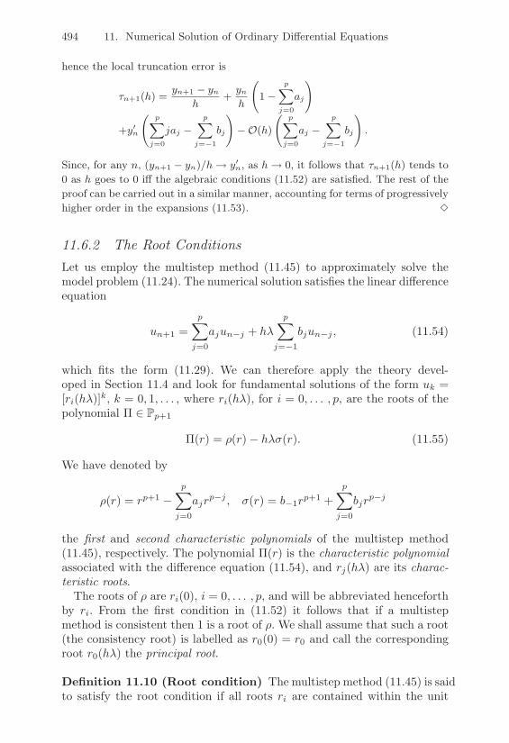
494 11. Numerical Solution of Ordinary Di"erential Equations
hence the local truncation error is
4n+1(h) =yn+1 % yn
h+
ynh
6
1%p(
j=0
aj
7
+y(n
6p(
j=0
jaj %p(
j=%1
bj
7
%O(h)
6p(
j=0
aj %p(
j=%1
bj
7
.
Since, for any n, (yn+1 % yn)/h, y(n, as h, 0, it follows that 4n+1(h) tends to
0 as h goes to 0 i" the algebraic conditions (11.52) are satisfied. The rest of theproof can be carried out in a similar manner, accounting for terms of progressivelyhigher order in the expansions (11.53). !
11.6.2 The Root ConditionsLet us employ the multistep method (11.45) to approximately solve themodel problem (11.24). The numerical solution satisfies the linear di!erenceequation
un+1 =p(
j=0
ajun"j + h$p(
j="1
bjun"j , (11.54)
which fits the form (11.29). We can therefore apply the theory devel-oped in Section 11.4 and look for fundamental solutions of the form uk =[ri(h$)]k, k = 0, 1, . . . , where ri(h$), for i = 0, . . . , p, are the roots of thepolynomial $ ! Pp+1
$(r) = )(r)" h$((r). (11.55)
We have denoted by
)(r) = rp+1 "p(
j=0
ajrp"j , ((r) = b"1rp+1 +
p(
j=0
bjrp"j
the first and second characteristic polynomials of the multistep method(11.45), respectively. The polynomial $(r) is the characteristic polynomialassociated with the di!erence equation (11.54), and rj(h$) are its charac-teristic roots.
The roots of ) are ri(0), i = 0, . . . , p, and will be abbreviated henceforthby ri. From the first condition in (11.52) it follows that if a multistepmethod is consistent then 1 is a root of ). We shall assume that such a root(the consistency root) is labelled as r0(0) = r0 and call the correspondingroot r0(h$) the principal root.
Definition 11.10 (Root condition) The multistep method (11.45) is saidto satisfy the root condition if all roots ri are contained within the unit

11.6 Analysis of Multistep Methods 495
circle centered at the origin of the complex plane, otherwise, if they fall onits boundary, they must be simple roots of ). Equivalently,
B|rj | & 1, j = 0, . . . , p;
furthermore, for those j such that |rj | = 1, then )*(rj) '= 0.(11.56)
!
Definition 11.11 (Strong root condition) The multistep method (11.45)is said to satisfy the strong root condition if it satisfies the root conditionand r0 = 1 is the only root lying on the boundary of the unit circle. Equiv-alently,
|rj | < 1 j = 1, . . . , p. (11.57)
!
Definition 11.12 (Absolute root condition) The multistep method(11.45) satisfies the absolute root condition if there exists h0 > 0 such that
|rj(h$)| < 1 j = 0, . . . , p, #h & h0.
!
11.6.3 Stability and Convergence Analysis for MultistepMethods
Let us now examine the relation between root conditions and the stabilityof multistep methods. Generalizing the Definition 11.4, we can get thefollowing.
Definition 11.13 (Zero-stability of multistep methods) The multi-step method (11.45) is zero-stable if
-h0 > 0, -C > 0 : #h ! (0, h0], |z(h)n " u(h)
n | & C+, 0 & n & Nh,(11.58)
where Nh = max {n : tn & t0 + T} and z(h)n and u(h)
n are, respectively, thesolutions of problems
)*+
*,
z(h)n+1 =
p(
j=0
ajz(h)n"j + h
p(
j="1
bjf(tn"j , z(h)n"j) + h%n+1,
z(h)k = w(h)
k + %k, k = 0, . . . , p
(11.59)
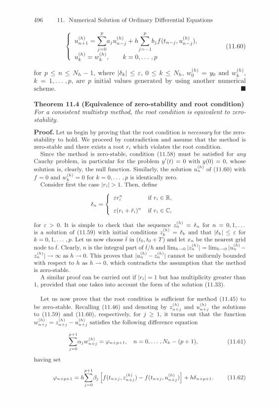
496 11. Numerical Solution of Ordinary Di"erential Equations
)*+
*,
u(h)n+1 =
p(
j=0
aju(h)n"j + h
p(
j="1
bjf(tn"j , u(h)n"j),
u(h)k = w(h)
k , k = 0, . . . , p
(11.60)
for p & n & Nh " 1, where |%k| & +, 0 & k & Nh, w(h)0 = y0 and w(h)
k ,k = 1, . . . , p, are p initial values generated by using another numericalscheme. !
Theorem 11.4 (Equivalence of zero-stability and root condition)For a consistent multistep method, the root condition is equivalent to zero-stability.
Proof. Let us begin by proving that the root condition is necessary for the zero-stability to hold. We proceed by contradiction and assume that the method iszero-stable and there exists a root ri which violates the root condition.
Since the method is zero-stable, condition (11.58) must be satisfied for anyCauchy problem, in particular for the problem y((t) = 0 with y(0) = 0, whosesolution is, clearly, the null function. Similarly, the solution u(h)
n of (11.60) withf = 0 and w(h)
k = 0 for k = 0, . . . , p is identically zero.Consider first the case |ri| > 1. Then, define
!n =
)+
,
&rni if ri / R,
&(ri + ri)n if ri / C,
for & > 0. It is simple to check that the sequence z(h)n = !n for n = 0, 1, . . .
is a solution of (11.59) with initial conditions z(h)k = !k and that |!k| " & for
k = 0, 1, . . . , p. Let us now choose t in (t0, t0 + T ) and let xn be the nearest gridnode to t. Clearly, n is the integral part of t/h and limh$0 |z(h)
n | = limh$0 |u(h)n %
z(h)n |,# as h, 0. This proves that |u(h)
n % z(h)n | cannot be uniformly bounded
with respect to h as h , 0, which contradicts the assumption that the methodis zero-stable.
A similar proof can be carried out if |ri| = 1 but has multiplicity greater than1, provided that one takes into account the form of the solution (11.33).
Let us now prove that the root condition is su!cient for method (11.45) tobe zero-stable. Recalling (11.46) and denoting by z(h)
n+j and u(h)n+j the solutions
to (11.59) and (11.60), respectively, for j ! 1, it turns out that the functionw(h)
n+j = z(h)n+j % u(h)
n+j satisfies the following di"erence equation
p+1(
j=0
$jw(h)n+j = (n+p+1, n = 0, . . . , Nh % (p + 1), (11.61)
having set
(n+p+1 = hp+1(
j=0
)j
Vf(tn+j , z
(h)n+j)% f(tn+j , u
(h)n+j)
W+ h!n+p+1. (11.62)
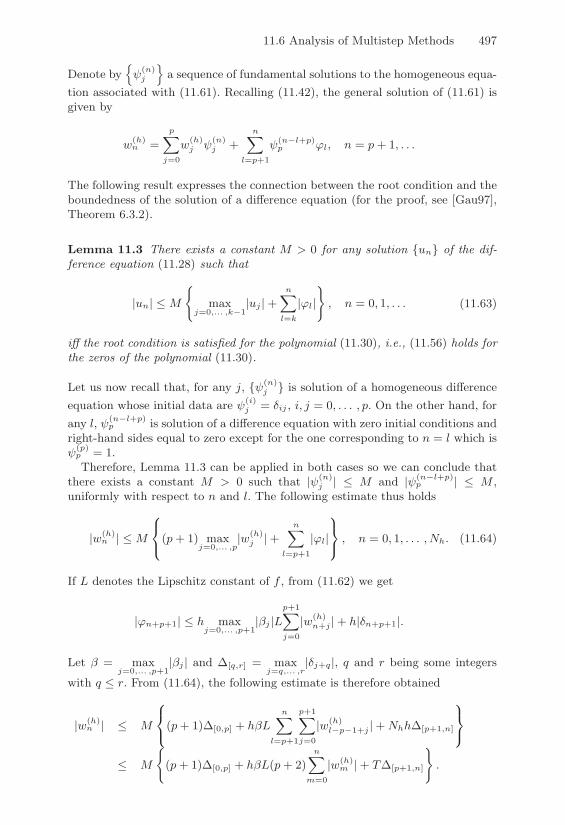
11.6 Analysis of Multistep Methods 497
Denote byR5(n)
j
Sa sequence of fundamental solutions to the homogeneous equa-
tion associated with (11.61). Recalling (11.42), the general solution of (11.61) isgiven by
w(h)n =
p(
j=0
w(h)j 5(n)
j +n(
l=p+1
5(n%l+p)p (l, n = p + 1, . . .
The following result expresses the connection between the root condition and theboundedness of the solution of a di"erence equation (for the proof, see [Gau97],Theorem 6.3.2).
Lemma 11.3 There exists a constant M > 0 for any solution {un} of the dif-ference equation (11.28) such that
|un| "M
B
maxj=0,... ,k%1
|uj | +n(
l=k
|(l|C
, n = 0, 1, . . . (11.63)
i! the root condition is satisfied for the polynomial (11.30), i.e., (11.56) holds forthe zeros of the polynomial (11.30).
Let us now recall that, for any j, {5(n)j } is solution of a homogeneous di"erence
equation whose initial data are 5(i)j = !ij , i, j = 0, . . . , p. On the other hand, for
any l, 5(n%l+p)p is solution of a di"erence equation with zero initial conditions and
right-hand sides equal to zero except for the one corresponding to n = l which is5(p)
p = 1.Therefore, Lemma 11.3 can be applied in both cases so we can conclude that
there exists a constant M > 0 such that |5(n)j | " M and |5(n%l+p)
p | " M ,uniformly with respect to n and l. The following estimate thus holds
|w(h)n | "M
)+
,(p + 1) maxj=0,... ,p
|w(h)j | +
n(
l=p+1
|(l|
_`
a , n = 0, 1, . . . , Nh. (11.64)
If L denotes the Lipschitz constant of f , from (11.62) we get
|(n+p+1| " h maxj=0,... ,p+1
|)j |Lp+1(
j=0
|w(h)n+j | + h|!n+p+1|.
Let ) = maxj=0,... ,p+1
|)j | and $[q,r] = maxj=q,... ,r
|!j+q|, q and r being some integers
with q " r. From (11.64), the following estimate is therefore obtained
|w(h)n | " M
)+
,(p + 1)$[0,p] + h)Ln(
l=p+1
p+1(
j=0
|w(h)l%p%1+j | + Nhh$[p+1,n]
_`
a
" M
B
(p + 1)$[0,p] + h)L(p + 2)n(
m=0
|w(h)m | + T$[p+1,n]
C
.
498 11. Numerical Solution of Ordinary Di"erential Equations
Let Q = 2(p + 2))LM and h0 = 1/Q, so that 1% hQ2 !
12 if h " h0. Then
12|w(h)
n | " |w(h)n |(1% hQ
2 )
" M
B
(p + 1)$[0,p] + h)L(p + 2)n%1(
m=0
|w(h)m | + T$[p+1,n]
C
.
Letting R = 2M/(p + 1)$[0,p] + T$[p+1,n]
0, we finally obtain
|w(h)n | " hQ
n%1(
m=0
|w(h)m | + R.
Applying Lemma 11.2 with the following identifications: (n = |w(h)n |, g0 = R,
ps = 0 and ks = hQ for any s = 0, . . . , n% 1, yields
|w(h)n | " 2MeTQ /
(p + 1)$[0,p] + T$[p+1,n]0. (11.65)
Method (11.45) is thus zero-stable for any h " h0. !
Theorem 11.4 allows for characterizing the stability behavior of severalfamilies of discretization methods.
In the special case of consistent one-step methods, the polynomial ) ad-mits only the root r0 = 1. They thus automatically satisfy the root conditionand are zero-stable.
For the Adams methods (11.49), the polynomial ) is always of the form)(r) = rp+1 " rp. Thus, its roots are r0 = 1 and r1 = 0 (with multiplicityp) so that all Adams methods are zero-stable.
Also the midpoint method (11.43) and Simpson method (11.44) are zero-stable: for both of them, the first characteristic polynomial is )(r) = r2"1,so that r0 = 1 and r1 = "1.
Finally, the BDF methods of Section 11.5.2 are zero-stable provided thatp & 5, since in such a case the root condition is satisfied (see [Cry73]).
We are in position to give the following convergence result.
Theorem 11.5 (Convergence) A consistent multistep method is conver-gent i! it satisfies the root condition and the error on the initial data tendsto zero as h ( 0. Moreover, the method converges with order q if it hasorder q and the error on the initial data tends to zero as O(hq).
Proof. Suppose that the MS method is consistent and convergent. To prove thatthe root condition is satisfied, we refer to the problem y((t) = 0 with y(0) = 0and on the interval I = (0, T ). Convergence means that the numerical solution{un} must tend to the exact solution y(t) = 0 for any converging set of initialdata uk, k = 0, . . . , p, i.e. max
k=0,... ,p|uk| , 0 as h , 0. From this observation, the
proof follows by contradiction along the same lines as the proof of Theorem 11.4,where the parameter & is now replaced by h.

11.6 Analysis of Multistep Methods 499
Let us now prove that consistency, together with the root condition, impliesconvergence under the assumption that the error on the initial data tends to zeroas h, 0. We can apply Theorem 11.4, setting u(h)
n = un (approximate solutionof the Cauchy problem) and z(h)
n = yn (exact solution), and from (11.47) it turnsout that !m = 4m(h). Then, due to (11.65), for any n ! p + 1 we obtain
|un % yn| " 2MeTQ
E(p + 1) max
j=0,... ,p|uj % yj | + T max
j=p+1,... ,n|4j(h)|
F.
Convergence holds by noticing that the right-hand side of this inequality tendsto zero as h, 0. !
A remarkable consequence of the above theorem is the following equivalenceLax-Richtmyer theorem.
Corollary 11.1 (Equivalence theorem) A consistent multistep methodis convergent i! it is zero-stable and if the error on the initial data tendsto zero as h tends to zero.
We conclude this section with the following result, which establishes anupper limit for the order of multistep methods (see [Dah63]).
Property 11.1 (First Dahlquist barrier) There isn’t any zero-stable,p-step linear multistep method with order greater than p + 1 if p is odd,p + 2 if p is even.
11.6.4 Absolute Stability of Multistep MethodsConsider again the di!erence equation (11.54), which was obtained by ap-plying the MS method (11.45) to the model problem (11.24). According to(11.33), its solution takes the form
un =k%(
j=1
6mj"1(
s=0
'sjns
7
[rj(h$)]n, n = 0, 1, . . .
where rj(h$), j = 1, . . . , k*, are the distinct roots of the characteristicpolynomial (11.55), and having denoted by mj the multiplicity of rj(h$).In view of (11.25), it is clear that the absolute root condition introducedby Definition 11.12 is necessary and su"cient to ensure that the multistepmethod (11.45) is absolutely stable as h & h0.
Among the methods enjoying the absolute stability property, the pref-erence should go to those for which the region of absolute stability A,introduced in (11.26), is as wide as possible or even unbounded. Amongthese are the A-stable methods introduced at the end of Section 11.3.3 and

500 11. Numerical Solution of Ordinary Di"erential Equations
the ,-stable methods, for which A contains the angular region defined byz ! C such that ", < & " arg(z) < ,, with , ! (0,&/2). A-stable meth-ods are of remarkable importance when solving sti! problems (see Section11.10).
Im
Re
Im
Re$
$
FIGURE 11.4. Regions of absolute stability for A-stable (left) and (right) "-stablemethods
The following result, whose proof is given in [Wid67], establishes a relationbetween the order of a multistep method, the number of its steps and itsstability properties.
Property 11.2 (Second Dahlquist barrier) A linear explicit multistepmethod can be neither A-stable, nor ,-stable. Moreover, there is no A-stable linear multistep method with order greater than 2. Finally, for any, ! (0,&/2), there only exist ,-stable p-step linear multistep methods oforder p for p = 3 and p = 4.
Let us now examine the region of absolute stability of several MS methods.
The regions of absolute stability of both explicit and implicit Adams schemesreduce progressively as the order of the method increases. In Figure 11.5(left) we show the regions of absolute stability for the AB methods exam-ined in Section 11.5.1, with exception of the Forward Euler method whoseregion is shown in Figura 11.3.
The regions of absolute stability of the Adams-Moulton schemes, exceptfor the Crank-Nicolson method which is A-stable, are represented in Figure11.5 (right).
In Figure 11.6 the regions of absolute stability of some of the BDF meth-ods introduced in Section 11.5.2 are drawn. They are unbounded and al-

11.6 Analysis of Multistep Methods 501
!2 !1.5 !1 !0.5 0!0.8
!0.6
!0.4
!0.2
0
0.2
0.4
0.6
0.8
AB2AB3
AB4
!6 !4 !2 0!4
!3
!2
!1
0
1
2
3
4
AM3
AM4AM5
FIGURE 11.5. Outer contours of the regions of absolute stability forAdams-Bashforth methods (left) ranging from second to fourth-order (AB2, AB3and AB4) and for Adams-Moulton methods (right), from third to fifth-order(AM3, AM4 and AM5). Notice that the region of the AB3 method extends intothe half-plane with positive real part. The region for the explicit Euler (AB1)method was drawn in Figure 11.3
ways contain the negative real numbers. These stability features make BDFmethods quite attractive for solving sti! problems (see Section 11.10).
!4 !2 0 2 4 6 8 10 12 14
!6
!4
!2
0
2
4
6
BDF6
BDF5
BDF3
FIGURE 11.6. Inner contours of regions of absolute stability for three-step(BDF3), five-step (BDF5) and six-step (BDF6) BDF methods. Unlike Adamsmethods, these regions are unbounded and extend outside the limited portionthat is shown in the figure
Remark 11.3 Some authors (see, e.g., [BD74]) adopt an alternative defi-nition of absolute stability by replacing (11.25) with the milder property
-C > 0 : |un| & C, as tn ( +,.
According to this new definition, the absolute stability of a numericalmethod should be regarded as the counterpart of the asymptotic stabil-

502 11. Numerical Solution of Ordinary Di"erential Equations
ity (11.6) of the Cauchy problem. The new region of absolute stability A,
would be
A, = {z ! C : -C > 0, |un| & C, #n ) 0}
and it would not necessarily coincide with A. For example, in the case ofthe midpoint method A is empty (thus, it is unconditionally absolutelyunstable), while A, = {z = "i, " ! ["1, 1]}.
In general, if A is nonempty, then A, is its closure. We notice that zero-stable methods are those for which the region A, contains the origin z = 0of the complex plane. !
To conclude, let us notice that the strong root condition (11.57) implies,for a linear problem, that
#h & h0, -C > 0 : |un| & C(|u0| + . . . + |up|), #n ) p + 1. (11.66)
We say that a method is relatively stable if it satisfies (11.66). Clearly,(11.66) implies zero-stability, but the converse does not hold.Figure 11.7 summarizes the main conclusions that have been drawn in thissection about stability, convergence and root-conditions, in the particularcase of a consistent method applied to the model problem (11.24).
Root A= Strong root A= Absolute rootcondition condition condition
cdedde
cde
Convergence A0 Zero A= (11.66) A= Absolutestability stability
FIGURE 11.7. Relations between root conditions, stability and convergence fora consistent method applied to the model problem (11.24)
11.7 Predictor-Corrector Methods
When solving a nonlinear Cauchy problem of the form (11.1), at each timestep implicit schemes require dealing with a nonlinear equation. For in-stance, if the Crank-Nicolson method is used, we get the nonlinear equation
un+1 = un +h
2[fn + fn+1] = )(un+1),

11.7 Predictor-Corrector Methods 503
that can be cast in the form '(un+1) = 0, where '(un+1) = un+1 ")(un+1). To solve this equation the Newton method would give
u(k+1)n+1 = u(k)
n+1 " '(u(k)n+1)/'
*(u(k)n+1),
for k = 0, 1, . . . , until convergence and require an initial datum u(0)n+1 su"-
ciently close to un+1. Alternatively, one can resort to fixed-point iterations
u(k+1)n+1 = )(u(k)
n+1) (11.67)
for k = 0, 1, . . . , until convergence. In such a case, the global convergencecondition for the fixed-point method (see Theorem 6.1) sets a constrainton the discretization stepsize of the form
h <1
|b"1|L(11.68)
where L is the Lipschitz constant of f with respect to y. In practice, ex-cept for the case of sti! problems (see Section 11.10), this restriction onh is not significant since considerations of accuracy put a much more re-strictive constraint on h. However, each iteration of (11.67) requires oneevaluation of the function f and the computational cost can be reduced byproviding a good initial guess u(0)
n+1. This can be done by taking one step ofan explicit MS method and then iterating on (11.67) for a fixed number mof iterations. By doing so, the implicit MS method that is employed in thefixed-point scheme “corrects” the value of un+1 “predicted” by the explicitMS method. A procedure of this sort is called a predictor-corrector method,or PC method. There are many ways in which a predictor-corrector methodcan be implemented.
In its basic version, the value u(0)n+1 is computed by an explicit p+1-step
method, called the predictor (here identified by the coe"cients {aj , bj})
[P ] u(0)n+1 =
p(
j=0
aju(1)n"j + h
p(
j=0
bjf(0)n"j ,
where f (0)k = f(tk, u
(0)k ) and u(1)
k are the solutions computed by the PCmethod at the previous steps or are the initial conditions. Then, we evaluatethe function f at the new point (tn+1, u
(0)n+1) (evaluation step)
[E] f (0)n+1 = f(tn+1, u
(0)n+1),
and finally, one single fixed-point iteration is carried out using an implicitMS scheme of the form (11.45)
[C] u(1)n+1 =
p(
j=0
aju(1)n"j + hb"1f
(0)n+1 + h
p(
j=0
bjf(0)n"j .
504 11. Numerical Solution of Ordinary Di"erential Equations
This second step of the procedure, which is actually explicit, is called thecorrector. The overall procedure is shortly denoted by PEC or P (EC)1method, in which P and C denote one application at time tn+1 of thepredictor and the corrector methods, respectively, while E indicates oneevaluation of the function f .
This strategy above can be generalized supposing to perform m > 1 iter-ations at each step tn+1. The corresponding methods are called predictor-multicorrector schemes and compute u(0)
n+1 at time step tn+1 using the pre-dictor in the following form
[P ] u(0)n+1 =
p(
j=0
aju(m)n"j + h
p(
j=0
bjf(m"1)n"j . (11.69)
Here m ) 1 denotes the (fixed) number of corrector iterations that arecarried out in the following steps [E], [C]: for k = 0, 1, . . . ,m" 1
[E] f (k)n+1 = f(tn+1, u
(k)n+1),
[C] u(k+1)n+1 =
p(
j=0
aju(m)n"j + hb"1f
(k)n+1 + h
p(
j=0
bjf(m"1)n"j .
These implementations of the predictor-corrector technique are referred toas P (EC)m. Another implementation, denoted by P (EC)mE, consists ofupdating at the end of the process also the function f and is given by
[P ] u(0)n+1 =
p(
j=0
aju(m)n"j + h
p(
j=0
bjf(m)n"j ,
and for k = 0, 1, . . . ,m" 1,
[E] f (k)n+1 = f(tn+1, u
(k)n+1),
[C] u(k+1)n+1 =
p(
j=0
aju(m)n"j + hb"1f
(k)n+1 + h
p(
j=0
bjf(m)n"j ,
followed by
[E] f (m)n+1 = f(tn+1, u
(m)n+1).
Example 11.8 Heun’s method (11.10) can be regarded as a predictor-correctormethod whose predictor is the forward Euler method, while the corrector is theCrank-Nicolson method.
Another example is provided by the Adams-Bashforth method of order 2(11.50) and the Adams-Moulton method of order 3 (11.51). Its corresponding

11.7 Predictor-Corrector Methods 505
PEC implementation is: given u(0)0 = u(1)
0 = u0, u(0)1 = u(1)
1 = u1 and f (0)0 =
f(t0, u(0)0 ), f (0)
1 = f(t1, u(0)1 ), compute for n = 1, 2, . . . ,
[P ] u(0)n+1 = u(1)
n +h2
V3f (0)
n % f (0)n%1
W,
[E] f (0)n+1 = f(tn+1, u
(0)n+1),
[C] u(1)n+1 = u(1)
n +h12
V5f (0)
n+1 + 8f (0)n % f (0)
n%1
W,
while the PECE implementation is: given u(0)0 = u(1)
0 = u0, u(0)1 = u(1)
1 = u1 andf (1)0 = f(t0, u(1)
0 ), f (1)1 = f(t1, u(1)
1 ), compute for n = 1, 2, . . . ,
[P ] u(0)n+1 = u(1)
n +h2
V3f (1)
n % f (1)n%1
W,
[E] f (0)n+1 = f(tn+1, u
(0)n+1),
[C] u(1)n+1 = u(1)
n +h12
V5f (0)
n+1 + 8f (1)n % f (1)
n%1
W,
[E] f (1)n+1 = f(tn+1, u
(1)n+1).
•
Before studying the convergence of predictor-corrector methods, we intro-duce a simplification in the notation. Usually the number of steps of thepredictor is greater than those of the corrector, so that we define the num-ber of steps of the predictor-corrector pair as being equal to the number ofsteps of the predictor. This number will be denoted henceforth by p. Owingto this definition we no longer demand that the coe"cients of the correctorsatisfy |ap| + |bp| '= 0. Consider for example the predictor-corrector pair
[P ] u(0)n+1 = u(1)
n + hf(tn"1, u(0)n"1),
[C] u(1)n+1 = u(1)
n + h2
Vf(tn, u
(0)n ) + f(tn+1, u
(0)n+1)
W,
for which p = 2 (even though the corrector is a one-step method). Conse-quently, the first and the second characteristic polynomials of the correctormethod will be )(r) = r2 " r and ((r) = (r2 + r)/2 instead of )(r) = r" 1and ((r) = (r + 1)/2.
In any predictor-corrector method, the truncation error of the predictorcombines with the one of the corrector, generating a new truncation errorwhich we are going to examine. Let q and q be, respectively, the orders of thepredictor and the corrector and assume that y ! C:q+1, where :q = max(q, q).

506 11. Numerical Solution of Ordinary Di"erential Equations
Then
y(tn+1) "p(
j=0
ajy(tn"j)" hp(
j=0
bjf(tn"j , yn"j)
= Cq+1hq+1y(q+1)(tn) + O(hq+2),
y(tn+1) "p(
j=0
ajy(tn"j)" hp(
j="1
bjf(tn"j , yn"j)
= Cq+1hq+1y(q+1)(tn) + O(hq+2),
where Cq+1, Cq+1 are the error constants of the predictor and the correctormethod respectively. The following result holds.
Property 11.3 Let the predictor method have order q and the correctormethod have order q. Then:
If q ) q (or q < q with m > q " q), then the predictor-corrector methodhas the same order and the same PLTE as the corrector.
If q < q and m = q" q, then the predictor-corrector method has the sameorder as the corrector, but di!erent PLTE.
If q < q and m & q" q" 1, then the predictor-corrector method has orderequal to q + m (thus less than q).
In particular, notice that if the predictor has order q" 1 and the correctorhas order q, the PEC su"ces to get a method of order q. Moreover, theP (EC)mE and P (EC)m schemes have always the same order and the samePLTE.
Combining the Adams-Bashforth method of order q with the correspond-ing Adams-Moulton method of the same order we obtain the so-called ABMmethod of order q. It is possible to estimate its PLTE as
Cq+1
C,q+1 " Cq+1
Ku(m)n+1 " u(0)
n+1
L,
where Cq+1 and C,q+1 are the error constants given in Table 11.1. Accord-
ingly, the steplength h can be decreased if the estimate of the PLTE exceedsa given tolerance and increased otherwise (for the adaptivity of the steplength in a predictor-corrector method, see [Lam91], pp.128–147).
Program 93 provides an implementation of the P (EC)mE methods. Theinput parameters at, bt, a, b contain the coe"cients aj , bj (j = 0, . . . , p)of the predictor and the coe"cients aj (j = 0, . . . , p), bj (j = "1, . . . , p) ofthe corrector. Moreover, f is a string containing the expression of f(t, y),

11.7 Predictor-Corrector Methods 507
h is the stepsize, t0 and tf are the end points of the time integrationinterval, u0 is the vector of the initial data, m is the number of the correctorinner iterations. The input variable pece must be set equal to ’y’ if theP (EC)mE is selected, conversely the P (EC)m scheme is chosen.
Program 93 - predcor : Predictor-corrector scheme
function [u,t]=predcor(a,b,at,bt,h,f,t0,u0,tf,pece,m)p = max(length(a),length(b)-1); pt = max(length(at),length(bt));q = max(p,pt); if length(u0) < q, break, end;t = [t0:h:t0+(q-1)*h]; u = u0; y = u0; fe = eval(f);k = q;for t = t0+q*h:h:tf
ut = sum(at.*u(k:-1:k-pt+1))+h*sum(bt.*fe(k:-1:k-pt+1));y = ut; foy = eval(f);uv = sum(a.*u(k:-1:k-p+1))+h*sum(b(2:p+1).*fe(k:-1:k-p+1));k = k+1;for j = 1:m
fy = foy; up = uv + h*b(1)*fy; y = up; foy = eval(f);endif (pece==’y’|pece==’Y’)
fe = [fe, foy];else
fe = [fe, fy];endu = [u, up];
endt = [t0:h:tf];
Example 11.9 Let us check the performance of the P (EC)mE method on theCauchy problem y((t) = e%y(t) for t / [0, 1] with y(0) = 1. The exact solution isy(t) = log(1 + t). In all the numerical experiments, the corrector method is theAdams-Moulton third-order scheme (AM3), while the explicit Euler (AB1) andthe Adams-Bashforth second-order (AB2) methods are used as predictors. Figure11.8 shows that the pair AB2-AM3 (m = 1) yields third-order convergence rate,while AB1-AM3 (m = 1) has a first-order accuracy. Taking m = 2 allows torecover the third-order convergence rate of the corrector for the AB1-AM3 pair.•
As for the absolute stability, the characteristic polynomial of P (EC)mmethods reads
$P (EC)m(r) = b"1rp (:)(r)" h$:((r)) +
Hm(1"H)1"Hm
()(r):((r)" :)(r)((r))
while for P (EC)mE we have
$P (EC)mE(r) = :)(r)" h$:((r) +Hm(1"H)
1"Hm()(r)" h$((r)) .
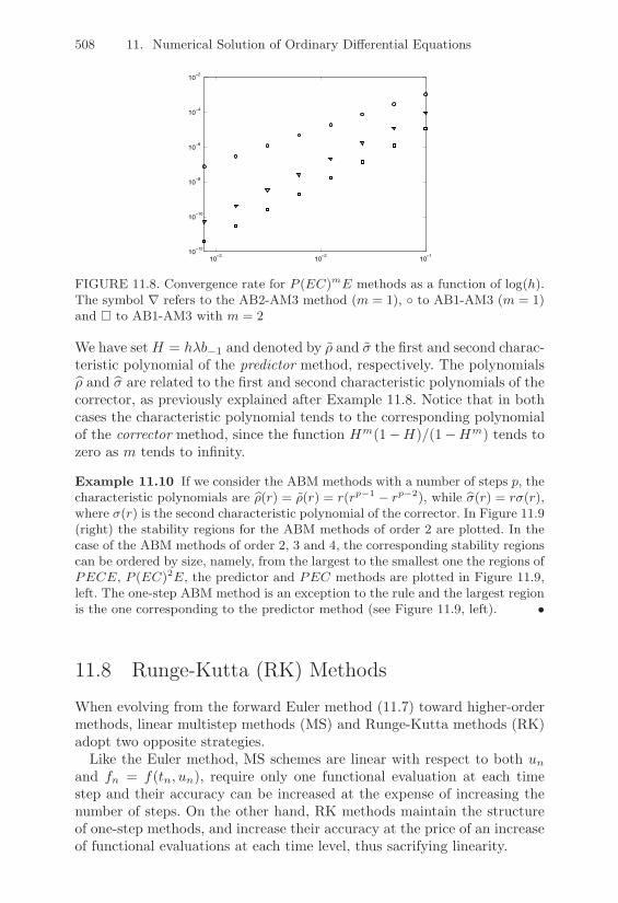
508 11. Numerical Solution of Ordinary Di"erential Equations
10!3
10!2
10!1
10!12
10!10
10!8
10!6
10!4
10!2
FIGURE 11.8. Convergence rate for P (EC)mE methods as a function of log(h).The symbol 8 refers to the AB2-AM3 method (m = 1), 9 to AB1-AM3 (m = 1)and # to AB1-AM3 with m = 2
We have set H = h$b"1 and denoted by ) and ( the first and second charac-teristic polynomial of the predictor method, respectively. The polynomials:) and :( are related to the first and second characteristic polynomials of thecorrector, as previously explained after Example 11.8. Notice that in bothcases the characteristic polynomial tends to the corresponding polynomialof the corrector method, since the function Hm(1"H)/(1"Hm) tends tozero as m tends to infinity.
Example 11.10 If we consider the ABM methods with a number of steps p, thecharacteristic polynomials are :%(r) = %(r) = r(rp%1 % rp%2), while :'(r) = r'(r),where '(r) is the second characteristic polynomial of the corrector. In Figure 11.9(right) the stability regions for the ABM methods of order 2 are plotted. In thecase of the ABM methods of order 2, 3 and 4, the corresponding stability regionscan be ordered by size, namely, from the largest to the smallest one the regions ofPECE, P (EC)2E, the predictor and PEC methods are plotted in Figure 11.9,left. The one-step ABM method is an exception to the rule and the largest regionis the one corresponding to the predictor method (see Figure 11.9, left). •
11.8 Runge-Kutta (RK) Methods
When evolving from the forward Euler method (11.7) toward higher-ordermethods, linear multistep methods (MS) and Runge-Kutta methods (RK)adopt two opposite strategies.
Like the Euler method, MS schemes are linear with respect to both un
and fn = f(tn, un), require only one functional evaluation at each timestep and their accuracy can be increased at the expense of increasing thenumber of steps. On the other hand, RK methods maintain the structureof one-step methods, and increase their accuracy at the price of an increaseof functional evaluations at each time level, thus sacrifying linearity.

11.8 Runge-Kutta (RK) Methods 509
!1.5 !1 !0.5 0 0.5!1.5
!1
!0.5
0
0.5
1
1.5
PECE
P(EC)2E
PEC
P(EC)2
!2 !1.5 !1 !0.5 0 0.5!2
!1.5
!1
!0.5
0
0.5
1
1.5
2
PECE
P(EC)2E
PEC
FIGURE 11.9. Stability regions for the ABM methods of order 1 (left) and 2(right)
A consequence is that RK methods are more suitable than MS methodsat adapting the stepsize, whereas estimating the local error for RK methodsis more di"cult than it is in the case of MS methods.In its most general form, an RK method can be written as
un+1 = un + hF (tn, un, h; f), n ) 0 (11.70)
where F is the increment function defined as follows
F (tn, un, h; f) =s(
i=1
biKi,
Ki = f(tn + cih, un + hs(
j=1
aijKj), i = 1, 2, . . . , s(11.71)
and s denotes the number of stages of the method. The coe"cients {aij},{ci} and {bi} fully characterize an RK method and are usually collected inthe so-called Butcher array
c1 a11 a12 . . . a1sc2 a21 a22 a2s...
.... . .
...cs as1 as2 . . . ass
b1 b2 . . . bs
orc A
bT
where A = (aij) ! Rs!s, b = (b1, . . . , bs)T ! Rs and c = (c1, . . . , cs)
T !Rs. We shall henceforth assume that the following condition holds
ci =s(
j=1
aij i = 1, . . . , s. (11.72)

510 11. Numerical Solution of Ordinary Di"erential Equations
If the coe"cients aij in A are equal to zero for j ) i, with i = 1, 2, . . . , s,then each Ki can be explicitly computed in terms of the i " 1 coe"cientsK1, . . . ,Ki"1 that have already been determined. In such a case the RKmethod is explicit. Otherwise, it is implicit and solving a nonlinear systemof size s is necessary for computing the coe"cients Ki.
The increase in the computational e!ort for implicit schemes makes theiruse quite expensive; an acceptable compromise is provided by RK semi-implicit methods, in which case aij = 0 for j > i so that each Ki is thesolution of the nonlinear equation
Ki = f
G
Htn + cih, un + haii Ki + hi"1(
j=1
aijKj
I
J .
A semi-implicit scheme thus requires s nonlinear independent equations tobe solved.
The local truncation error 5n+1(h) at node tn+1 of the RK method(11.70) is defined through the residual equation
h5n+1(h) = yn+1 " yn " hF (tn, yn, h; f),
where y(t) is the exact solution to the Cauchy problem (11.1). Method(11.70) is consistent if 5(h) = maxn |5n(h)|( 0 as h( 0. It can be shown(see [Lam91]) that this happens i!
s(
i=1
bi = 1.
As usual, we say that (11.70) is a method of order p () 1) with respect toh if 5(h) = O(hp) as h( 0.
As for convergence, since RK methods are one-step methods, consistencyimplies stability and, in turn, convergence. As happens for MS methods,estimates of 5(h) can be derived; however, these estimates are often toocomplicated to be profitably used. We only mention that, as for MS meth-ods, if an RK scheme has a local truncation error 5n(h) = O(hp), for anyn, then also the convergence order will be equal to p.
The following result establishes a relation between order and number ofstages of explicit RK methods.
Property 11.4 The order of an s-stage explicit RK method cannot begreater than s. Also, there do not exist s-stage explicit RK methods withorder s ) 5.
We refer the reader to [But87] for the proofs of this result and the results wegive below. In particular, for orders ranging between 1 and 10, the minimum

11.8 Runge-Kutta (RK) Methods 511
number of stages smin required to get a method of corresponding order isshown below
order 1 2 3 4 5 6 7 8smin 1 2 3 4 6 7 9 11
Notice that 4 is the maximum number of stages for which the order of themethod is not less than the number of stages itself. An example of a fourth-order RK method is provided by the following explicit 4-stage method
un+1 = un +h
6(K1 + 2K2 + 2K3 + K4)
K1 = fn,
K2 = f(tn + h2 , un + h
2K1),
K3 = f(tn + h2 , un + h
2K2),
K4 = f(tn+1, un + hK3).
(11.73)
As far as implicit schemes are concerned, the maximum achievable orderusing s stages is equal to 2s.
Remark 11.4 (The case of systems of ODEs) An RK method can bereadily extended to systems of ODEs. However, the order of an RK methodin the scalar case does not necessarily coincide with that in the vectorcase. In particular, for p ) 4, a method having order p in the case of theautonomous system y* = f(y), with f : Rm ( Rn maintains order p evenwhen applied to an autonomous scalar equation y* = f(y), but the converseis not true. Regarding this concern, see [Lam91], Section 5.8. !
11.8.1 Derivation of an Explicit RK MethodThe standard technique for deriving an explicit RK method consists of en-forcing that the highest number of terms in Taylor’s expansion of the exactsolution yn+1 about tn coincide with those of the approximate solutionun+1, assuming that we take one step of the RK method starting from theexact solution yn. We provide an example of this technique in the case ofan explicit 2-stage RK method.
Let us consider a 2-stage explicit RK method and assume to dispose atthe n-th step of the exact solution yn. Then
un+1 = yn + hF (tn, yn, h; f) = yn + h(b1K1 + b2K2),
K1 = fn, K2 = f(tn + hc2, yn + hc2K1),
having assumed that (11.72) is satisfied. Expanding K2 in a Taylor seriesin a neighborhood of tn and truncating the expansion at the second order,

512 11. Numerical Solution of Ordinary Di"erential Equations
we get
K2 = fn + hc2(fn,t + K1fn,y) + O(h2).
We have denoted by fn,z (for z = t or z = y) the partial derivative of fwith respect to z evaluated at (tn, yn). Then
un+1 = yn + hfn(b1 + b2) + h2c2b2(fn,t + fnfn,y) + O(h3).
If we perform the same expansion on the exact solution, we find
yn+1 = yn + hy*n +h2
2y**n + O(h3) = yn + hfn +
h2
2(fn,t + fnfn,y) + O(h3).
Forcing the coe"cients in the two expansions above to agree, up to higher-order terms, we obtain that the coe"cients of the RK method must satisfyb1 + b2 = 1, c2b2 = 1
2 .Thus, there are infinitely many 2-stage explicit RK methods with second-
order accuracy. Two examples are the Heun method (11.10) and the modi-fied Euler method (11.91). Of course, with similar (and cumbersome) com-putations in the case of higher-stage methods, and accounting for a highernumber of terms in Taylor’s expansion, one can generate higher-order RKmethods. For instance, retaining all the terms up to the fifth one, we getscheme (11.73).
11.8.2 Stepsize Adaptivity for RK MethodsSince RK schemes are one-step methods, they are well-suited to adaptingthe stepsize h, provided that an e"cient estimator of the local error isavailable. Usually, a tool of this kind is an a posteriori error estimator,since the a priori local error estimates are too complicated to be used inpractice. The error estimator can be constructed in two ways:
- using the same RK method, but with two di!erent stepsizes (typically 2hand h);- using two RK methods of di!erent order, but with the same number s ofstages.
In the first case, if an RK method of order p is being used, one pretendsthat, starting from an exact datum un = yn (which would not be availableif n ) 1), the local error at tn+1 is less than a fixed tolerance. The followingrelation holds
yn+1 " un+1 = '(yn)hp+1 + O(hp+2), (11.74)
where ' is an unknown function evaluated at yn. (Notice that, in thisspecial case, yn+1 " un+1 = h5n+1(h)).

11.8 Runge-Kutta (RK) Methods 513
Carrying out the same computation with a stepsize of 2h, starting fromtn"1, and denoting by :un+1 the computed solution, yields
yn+1 " :un+1 = '(yn"1)(2h)p+1 + O(hp+2) = '(yn)(2h)p+1 + O(hp+2)(11.75)
having expanded also yn"1 with respect to tn. Subtracting (11.74) from(11.75), we get
(2p+1 " 1)hp+1'(yn) = un+1 " :un+1 + O(hp+2),
from which
yn+1 " un+1 1un+1 " :un+1
(2p+1 " 1)= E .
If |E| is less than the fixed tolerance +, the scheme moves to the next timestep, otherwise the estimate is repeated with a halved stepsize. In general,the stepsize is doubled whenever |E| is less than +/2p+1.
This approach yields a considerable increase in the computational e!ort,due to the s" 1 extra functional evaluations needed to generate the value:un+1. Moreover, if one needs to half the stepsize, the value un must alsobe computed again.
An alternative that does not require extra functional evaluations consistsof using simultaneously two di!erent RK methods with s stages, of orderp and p + 1, respectively, which share the same set of values Ki. Thesemethods are synthetically represented by the modified Butcher array
c AbT 2
:bT 2
ET 2
(11.76)
where the method of order p is identified by the coe"cients c, A and b,while that of order p+ 1 is identified by c, A and :b, and where E = b" :b.
Taking the di!erence between the approximate solutions at tn+1 pro-duced by the two methods provides an estimate of the local truncationerror for the scheme of lower order. On the other hand, since the coe"-cients Ki coincide, this di!erence is given by h
!si=1 EiKi and thus it does
not require extra functional evaluations.Notice that, if the solution un+1 computed by the scheme of order p is
used to initialize the scheme at time step n+2, the method will have orderp, as a whole. If, conversely, the solution computed by the scheme of orderp+1 is employed, the resulting scheme would still have order p+1 (exactlyas happens with predictor-corrector methods).
The Runge-Kutta Fehlberg method of fourth-order is one of the mostpopular schemes of the form (11.76) and consists of a fourth-order RK

514 11. Numerical Solution of Ordinary Di"erential Equations
scheme coupled with a fifth-order RK method (for this reason, it is knownas the RK45 method). The modified Butcher array for this method is shownbelow
0 0 0 0 0 0 014
14 0 0 0 0 0
38
332
932 0 0 0 0
1213
19322197 " 7200
219772962197 0 0 0
1 439216 "8 3680
513 " 8454104 0 0
12 " 8
27 2 " 35442565
18594104 " 11
40 0
25216 0 1408
256521974104 " 1
5 016135 0 6656
128252856156430 " 9
50255
1360 0 " 128
4275 " 219775240
150
255
This method tends to underestimate the error. As such, its use is not com-pletely reliable when the stepsize h is large.
Remark 11.5 MATLAB provides a package tool funfun, which, besidesthe two classical Runge-Kutta Fehlberg methods, RK23 (second-order andthird-order pair) and RK45 (fourth-order and fifth-order pair), also imple-ments other methods suitable for solving sti! problems. These methods arederived from BDF methods (see [SR97]) and are included in the MATLABprogram ode15s. !
11.8.3 Implicit RK MethodsImplicit RK methods can be derived from the integral formulation of theCauchy problem (11.2). In fact, if a quadrature formula with s nodes in(tn, tn+1) is employed to approximate the integral of f (which we assume,for simplicity, to depend only on t), we get
tn+1^
tn
f(5) d5 1 hs(
j=1
bjf(tn + cjh)
having denoted by bj the weights and by tn + cjh the quadrature nodes. Itcan be proved (see [But64]) that for any RK formula (11.70)-(11.71), thereexists a correspondence between the coe"cients bj , cj of the formula andthe weights and nodes of a Gauss quadrature rule.
In particular, the coe"cients c1, . . . , cs are the roots of the Legendrepolynomial Ls in the variable x = 2c " 1, so that x ! ["1, 1]. Once the

11.8 Runge-Kutta (RK) Methods 515
s coe"cients cj have been found, we can construct RK methods of order2s, by determining the coe"cients aij and bj as being the solutions of thelinear systems
s(
j=1
ck"1j aij = (1/k)cki , k = 1, 2, . . . , s,
s(
j=1
ck"1j bj = 1/k, k = 1, 2, . . . , s.
The following families can be derived:
1. Gauss-Legendre RK methods, if Gauss-Legendre quadrature nodes areused. These methods, for a fixed number of stages s, attain the maximumpossible order 2s. Remarkable examples are the one-stage method (implicitmidpoint method) of order 2
un+1 = un + hf8tn + 1
2h,12 (un + un+1)
9,
12
12
1
and the 2-stage method of order 4, described by the following Butcher array
3"(
36
14
3"2(
312
3+(
36
3+2(
312
14
12
12
2. Gauss-Radau methods, which are characterized by the fact that thequadrature nodes include one of the two endpoints of the interval (tn, tn+1).The maximum order that can be achieved by these methods is 2s"1, whens stages are used. Elementary examples correspond to the following Butcherarrays
0 11 ,
1 11 ,
13
512 " 1
12
1 34
14
34
14
and have order 1, 1 and 3, respectively. The Butcher array in the middlerepresents the backward Euler method.
3. Gauss-Lobatto methods, where both the endpoints tn and tn+1 are quadra-ture nodes. The maximum order that can be achieved using s stages is2s" 2. We recall the methods of the family corresponding to the following

516 11. Numerical Solution of Ordinary Di"erential Equations
Butcher arrays
0 0 01 1
212
12
12
,
0 12 0
1 12 0
12
12
,
0 16 " 1
316
12
16
512 " 1
12
1 16
23
16
16
23
16
which have order 2, 2 and 3, respectively. The first array represents theCrank-Nicolson method.
As for semi-implicit RK methods, we limit ourselves to mentioning thecase of DIRK methods (diagonally implicit RK), which, for s = 3, arerepresented by the following Butcher array
1+µ2
1+µ2 0 0
12 "µ
21+µ
2 01"µ
2 1 + µ "1" 2µ 1+µ2
16µ2 1" 1
3µ21
6µ2
The parameter µ represents one of the three roots of 3µ3"3µ"1 = 0 (i.e.,(2//
3) cos(10o), "(2//
3) cos(50o), "(2//
3) cos(70o)). The maximum or-der that has been determined in the literature for these methods is 4.
11.8.4 Regions of Absolute Stability for RK MethodsApplying an s-stage RK method to the model problem (11.24) yields
Ki = un + h$s(
i=1
aijKj , un+1 = un + h$s(
i=1
biKi, (11.77)
that is, a first-order di!erence equation. If K and 1 are the vectors of com-ponents (K1, . . . ,Ks)T and (1, . . . , 1)T , respectively, then (11.77) becomes
K = un1 + h$AK, un+1 = un + h$bTK,
from which, K = (I" h$A)"11un and thus
un+1 =P1 + h$bT (I" h$A)"11
Qun = R(h$)un
where R(h$) is the so-called stability function.The RK method is absolutely stable, i.e., the sequence {un} satisfies
(11.25), i! |R(h$)| < 1. Its region of absolute stability is given by
A = {z = h$ ! C such that |R(h$)| < 1} .

11.9 Systems of ODEs 517
If the method is explicit, A is strictly lower triangular and the function Rcan be written in the following form (see [DV84])
R(h$) =det(I" h$A + h$1bT )
det(I" h$A).
Thus since det(I"h$A) = 1, R(h$) is a polynomial function in the variableh$, |R(h$)| can never be less than 1 for all values of h$. Consequently, Acan never be unbounded for an explicit RK method.
In the special case of an explicit RK of order s = 1, . . . , 4, one gets (see[Lam91])
R(h$) =s(
k=0
1k!
(h$)k.
The corresponding regions of absolute stability are drawn in Figure 11.10.Notice that, unlike MS methods, the regions of absolute stability of RKmethods increase in size as the order grows.
!4 !3 !2 !1 0 1 20
0.5
1
1.5
2
2.5
3
3.5
4
s=1
s=2
s=4
s=3
FIGURE 11.10. Regions of absolute stability for s-stage explicit RK methods,with s = 1, . . . , 4. The plot only shows the portion Im(h#) ! 0 since the regionsare symmetric about the real axis
We finally notice that the regions of absolute stability for explicit RK meth-ods can fail to be connected; an example is given in Exercise 14.
11.9 Systems of ODEs
Let us consider the system of first-order ODEs
y* = F(t,y), (11.78)
where F : R % Rn ( Rn is a given vector function and y ! Rn is thesolution vector which depends on n arbitrary constants set by the n initial

518 11. Numerical Solution of Ordinary Di"erential Equations
conditions
y(t0) = y0. (11.79)
Let us recall the following property (see [PS91], p. 209).
Property 11.5 Let F : R % Rn ( Rn be a continuous function on D =[t0, T ] % Rn, with t0 and T finite. Then, if there exists a positive constantL such that
+F(t,y)" F(t, y)+ & L+y " y+ (11.80)
holds for any (t,y) and (t, y) ! D, then, for any y0 ! Rn there exists aunique y, continuous and di!erentiable with respect to t for any (t,y) ! D,which is a solution of the Cauchy problem (11.78)-(11.79).
Condition (11.80) expresses the fact that F is Lipschitz continuous withrespect to the second argument.
It is seldom possible to write out in closed form the solution to system(11.78). A special case is where the system takes the form
y*(t) = Ay(t), (11.81)
with A! Rn!n. Assume that A has n distinct eigenvalues $j , j = 1, . . . , n;therefore, the solution y can be written as
y(t) =n(
j=1
Cje#jtvj , (11.82)
where C1, . . . , Cn are some constants and {vj} is a basis formed by theeigenvectors of A, associated with the eigenvalues $j for j = 1, . . . , n. Thesolution is determined by setting n initial conditions.
From the numerical standpoint, the methods introduced in the scalarcase can be extended to systems. A delicate matter is how to generalize thetheory developed about absolute stability.
With this aim, let us consider system (11.81). As previously seen, theproperty of absolute stability is concerned with the behavior of the numer-ical solution as t grows to infinity, in the case where the solution of problem(11.78) satisfies
+y(t)+ ( 0 as t(,. (11.83)
Condition (11.83) is satisfied if all the real parts of the eigenvalues of A arenegative since this ensures that
e#jt = eRe#jt(cos(Im$j) + i sin(Im$i)) ( 0, as t(,, (11.84)

11.10 Sti" Problems 519
from which (11.83) follows recalling (11.82). Since A has n distinct eigen-values, there exists a nonsingular matrix Q such that % = Q"1AQ, % beingthe diagonal matrix whose entries are the eigenvalues of A (see Section 1.8).
Introducing the auxiliary variable z = Q"1y, the initial system can there-fore be transformed into
z* = %z. (11.85)
Since % is a diagonal matrix, the results holding in the scalar case immedi-ately apply to the vector case as well, provided that the analysis is repeatedon all the (scalar) equations of system (11.85).
11.10 Sti" Problems
Consider a nonhomogeneous linear system of ODEs with constant coe"-cients
y*(t) = Ay(t) + )(t), with A ! Rn!n, )(t) ! Rn,
and assume that A has n distinct eigenvalues $j , j = 1, . . . , n. Then
y(t) =n(
j=1
Cje#jtvj + *(t)
where C1, . . . , Cn, are n constants, {vj} is a basis formed by the eigenvec-tors of A and *(t) is a particular solution of the ODE at hand. Throughoutthe section, we assume that Re$j < 0 for all j.
As t ( ,, the solution y tends to the particular solution *. We cantherefore interpret * as the steady-state solution (that is, after an infinite
time) andn(
j=1
Cje#jt as being the transient solution (that is, for t finite).
Assume that we are interested only in the steady-state. If we employ anumerical scheme with a bounded region of absolute stability, the stepsize his subject to a constraint that depends on the maximum module eigenvalueof A. On the other hand, the greater this module, the shorter the timeinterval where the corresponding component in the solution is meaningful.We are thus faced with a sort of paradox: the scheme is forced to employa small integration stepsize to track a component of the solution that isvirtually flat for large values of t.
Precisely, if we assume that
( & Re$j & 5 < 0, #j = 1, . . . , n (11.86)
and introduce the sti!ness quotient rs = (/5 , we say that a linear systemof ODEs with constant coe"cients is sti! if the eigenvalues of matrix A allhave negative real parts and rs 4 1.

520 11. Numerical Solution of Ordinary Di"erential Equations
However, referring only to the spectrum of A to characterize the sti!ness ofa problem might have some drawbacks. For instance, when 5 1 0, the sti!-ness quotient can be very large while the problem appears to be “genuinely”sti! only if |(| is very large. Moreover, enforcing suitable initial conditionscan a!ect the sti!ness of the problem (for example, selecting the data insuch a way that the constants multiplying the “sti!” components of thesolution vanish).
For this reason, several authors find the previous definition of a sti!problem unsatisfactory, and, on the other hand, they agree on the fact thatit is not possible to exactly state what it is meant by a sti! problem. Welimit ourselves to quoting only one alternative definition, which is of someinterest since it focuses on what is observed in practice to be a sti! problem.
Definition 11.14 (from [Lam91], p. 220) A system of ODEs is sti! if,when approximated by a numerical scheme characterized by a region ofabsolute stability with finite size, it forces the method, for any initial con-dition for which the problem admits a solution, to employ a discretizationstepsize excessively small with respect to the smoothness of the exact so-lution. !From this definition, it is clear that no conditionally absolute stable methodis suitable for approximating a sti! problem. This prompts resorting toimplicit methods, such as MS or RK, which are more expensive than explicitschemes, but have regions of absolute stability of infinite size. However, itis worth recalling that, for nonlinear problems, implicit methods lead tononlinear equations, for which it is thus crucial to select iterative numericalmethods free of limitations on h for convergence.
For instance, in the case of MS methods, we have seen that using fixed-point iterations sets the constraint (11.68) on h in terms of the Lipschitzconstant L of f . In the case of a linear system this constraint is
L ) maxi=1,... ,n
|$i|,
so that (11.68) would imply a strong limitation on h (which could evenbe more stringent than those required for an explicit scheme to be stable).One way of circumventing this drawback consists of resorting to Newton’smethod or some variants. The presence of Dahlquist barriers imposes astrong limitation on the use of MS methods, the only exception being BDFmethods, which, as already seen, are !-stable for p & 5 (for a larger numberof steps they are even not zero-stable). The situation becomes definitelymore favorable if implicit RK methods are considered, as observed at theend of Section 11.8.4.
The theory developed so far holds rigorously if the system is linear. Inthe nonlinear case, let us consider the Cauchy problem (11.78), where the

11.11 Applications 521
function F : R % Rn ( Rn is assumed to be di!erentiable. To study itsstability a possible strategy consists of linearizing the system as
y*(t) = F(5,y(5)) + JF(5,y(5)) [y(t)" y(5)] ,
in a neighborhood (5,y(5)), where 5 is an arbitrarily chosen value of twithin the time integration interval.
The above technique might be dangerous since the eigenvalues of JF donot su"ce in general to describe the behavior of the exact solution of theoriginal problem. Actually, some counterexamples can be found where:
1. JF has complex conjugate eigenvalues, while the solution of (11.78)does not exhibit oscillatory behavior;
2. JF has real nonnegative eigenvalues, while the solution of (11.78) doesnot grow monotonically with t;
3. JF has eigenvalues with negative real parts, but the solution of (11.78)does not decay monotonically with t.
As an example of the case at item 3. let us consider the system ofODEs
y* =
"
#$" 1
2t2t3
" t
2" 1
2t
%
&'y = A(t)y.
For t ) 1 its solution is
y(t) = C1
-t"3/2
" 12 t
1/2
.+ C2
-2t"3/2 log tt1/2(1" log t)
.
whose Euclidean norm diverges monotonically for t > (12)1/4 1 1.86when C1 = 1, C2 = 0, whilst the eigenvalues of A(t), equal to ("1 ±2i)/(2t), have negative real parts.
Therefore, the nonlinear case must be tackled using ad hoc techniques, bysuitably reformulating the concept of stability itself (see [Lam91], Chapter7).
11.11 Applications
We consider two examples of dynamical systems that are well-suited tochecking the performances of several numerical methods introduced in theprevious sections.

522 11. Numerical Solution of Ordinary Di"erential Equations
11.11.1 Analysis of the Motion of a Frictionless PendulumLet us consider the frictionless pendulum in Figure 11.11 (left), whosemotion is governed by the following system of ODEs
By*1 = y2,
y*2 = "K sin(y1),(11.87)
for t > 0, where y1(t) and y2(t) represent the position and angular velocityof the pendulum at time t, respectively, while K is a positive constantdepending on the geometrical-mechanical parameters of the pendulum. Weconsider the initial conditions: y1(0) = !0, y2(0) = 0.
yweight1
A
A’ ! % K1/2
% K1/2
FIGURE 11.11. Left: frictionless pendulum; right: orbits of system (11.87) in thephase space
Denoting by y = (y1, y2)T the solution to system (11.87), this admitsinfinitely many equilibrium conditions of the form y = (n&, 0)T for n ! Z,corresponding to the situations where the pendulum is vertical with zerovelocity. For n even, the equilibrium is stable, while for n odd it is unstable.These conclusions can be drawn by analyzing the linearized system
y* = Aey =
N0 1
"K 0
O
y, y* = Aoy =
N0 1
K 0
O
y.
If n is even, matrix Ae has complex conjugate eigenvalues $1,2 = ±i/K
and associated eigenvectors y1,2 = (<i//K, 1)T , while for n odd, Ao
has real and opposite eigenvalues $1,2 = ±/K and eigenvectors y1,2 =
(1//K,<1)T .
Let us consider two di!erent sets of initial data: y(0) = (!0, 0)T andy(0) = (& + !0, 0)T , where |!0| : 1. The solutions of the correspondinglinearized system are, respectively,B
y1(t) = !0 cos(/Kt)
y2(t) = "/K!0 sin(
/Kt)
,
By1(t) = (& + !0) cosh(
/Kt)
y2(t) =/K(& + !0) sinh(
/Kt),

11.11 Applications 523
and will be henceforth denoted as “stable” and “unstable”, respectively, forreasons that will be clear later on. To these solutions we associate in theplane (y1, y2), called the phase space, the following orbits (i.e., the graphsobtained plotting the curve (y1(t), y2(t)) in the phase space).
4y1
!0
52
+4
y2/K!0
52
= 1, (stable case)4
y1
& + !0
52
"4
y2/K(& + !0)
52
= 1, (unstable case).
In the stable case, the orbits are ellipses with period 2&//K and are cen-
tered at (0, 0)T , while in the unstable case they are hyperbolae centered at(0, 0)T and asymptotic to the straight lines y2 = ±
/Ky1.
The complete picture of the motion of the pendulum in the phase spaceis shown in Figure 11.11 (right). Notice that, letting v = |y2| and fixingthe initial position y1(0) = 0, there exists a limit value vL = 2
/K which
corresponds in the figure to the points A and A’. For v(0) < vL, the orbitsare closed, while for v(0) > vL they are open, corresponding to a continuousrevolution of the pendulum, with infinite passages (with periodic and nonnull velocity) through the two equilibrium positions y1 = 0 and y1 = &.The limit case v(0) = vL yields a solution such that, thanks to the totalenergy conservation principle, y2 = 0 when y1 = &. Actually, these twovalues are attained asymptotically only as t(,.The first-order nonlinear di!erential system (11.87) has been numericallysolved using the forward Euler method (FE), the midpoint method (MP)and the Adams-Bashforth second-order scheme (AB). In Figure 11.12 weshow the orbits in the phase space that have been computed by the twomethods on the time interval (0, 30) and taking K = 1 and h = 0.1. Thecrosses denote initial conditions.
As can be noticed, the orbits generated by FE do not close. This kindof instability is due to the fact that the region of absolute stability of theFE method completely excludes the imaginary axis. On the contrary, theMP method describes accurately the closed system orbits due to the factthat its region of asymptotic stability (see Section 11.6.4) includes pureimaginary eigenvalues in the neighborhood of the origin of the complexplane. It must also be noticed that the MP scheme gives rise to oscillatingsolutions as v0 gets larger. The second-order AB method, instead, describescorrectly all kinds of orbits.
11.11.2 Compliance of Arterial WallsAn arterial wall subject to blood flow can be modelled by a compliantcircular cylinder of length L and radius R0 with walls made by an incom-pressible, homogeneous, isotropic, elastic tissue of thickness H. A simple

524 11. Numerical Solution of Ordinary Di"erential Equations
!10 !5 0 5 10
!2
0
2
!10 !5 0 5 10
!2
0
2
!10 !5 0 5 10
!2
0
2
FIGURE 11.12. Orbits for system (11.87) in the case K = 1 and h = 0.1, com-puted using the FE method (upper plot), the MP method (central plot) and theAB method (lower plot), respectively. The initial conditions are .0 = +/10 andv0 = 0 (thin solid line), v0 = 1 (dashed line), v0 = 2 (dash-dotted line) andv0 = %2 (thick solid line)
model describing the mechanical behavior of the walls interacting with theblood flow is the so called “independent-rings” model according to whichthe vessel wall is regarded as an assembly of rings which are not influencedone by the others.
This amounts to neglecting the longitudinal (or axial) inner actions alongthe vessel, and to assuming that the walls can deform only in the radialdirection. Thus, the vessel radius R is given by R(t) = R0 +y(t), where y isthe radial deformation of the ring with respect to a reference radius R0 andt is the time variable. The application of Newton’s law to the independent-ring system yields the following equation modeling the time mechanical
11.11 Applications 525
behavior of the wall
y**(t) + #y*(t) + "y(t) = '(p(t)" p0) (11.88)
where " = E/()wR20), ' = 1/()wH) and # is a positive constant. The
physical parameters )w and E denote the vascular wall density and theYoung modulus of the vascular tissue, respectively. The function p " p0is the forcing term acting on the wall due to the pressure drop betweenthe inner part of the vessel (where the blood flows) and its outer part(surrounding organs). At rest, if p = p0, the vessel configuration coincideswith the undeformed circular cylinder having radius equal exactly to R0(y = 0).
Equation (11.88) can be formulated as y*(t) = Ay(t) + b(t) where y =(y, y*)T , b = (0,"'(p" p0))T and
A =
60 1
"" "#
7
. (11.89)
The eigenvalues of A are $± = ("# ±3#2 " 4")/2; therefore, if # ) 2
/"
both the eigenvalues are real and negative and the system is asymptoticallystable with y(t) decaying exponentially to zero as t(,. Conversely, if 0 <# < 2
/" the eigenvalues are complex conjugate and damped oscillations
arise in the solution which again decays exponentially to zero as t(,.Numerical approximations have been carried out using both the backwardEuler (BE) and Crank-Nicolson (CN) methods. We have set y(t) = 0and used the following (physiological) values of the physical parameters:L = 5 · 10"2[m], R0 = 5 · 10"3[m], )w = 103[Kgm"3], H = 3 · 10"4[m] andE = 9 · 105[Nm"2], from which ' 1 3.3[Kg"1m"2] and " = 36 · 106[s"2].A sinusoidal function p" p0 = x#p(a+ b cos(00t)) has been used to modelthe pressure variation along the vessel direction x and time, where #p =0.25 · 133.32 [Nm"2], a = 10 · 133.32 [Nm"2], b = 133.32 [Nm"2] and thepulsation 00 = 2&/0.8 [rad s"1] corresponds to a heart beat.
The results reported below refer to the ring coordinate x = L/2. Thetwo (very di!erent) cases (1) # =
/" [s"1] and (2) # = " [s"1] have been
analyzed; it is easily seen that in case (2) the sti!ness quotient (see Section11.10) is almost equal to ", thus the problem is highly sti!. We notice alsothat in both cases the real parts of the eigenvalues of A are very large,so that an appropriately small time step should be taken to accuratelydescribe the fast transient of the problem.In case (1) the di!erential system has been studied on the time interval[0, 2.5 ·10"3] with a time step h = 10"4. We notice that the two eigenvaluesof A have modules equal to 6000, thus our choice of h is compatible withthe use of an explicit method as well.
Figure 11.13 (left) shows the numerical solutions as functions of time.The solid (thin) line is the exact solution while the thick dashed and solid

526 11. Numerical Solution of Ordinary Di"erential Equations
lines are the solutions given by the CN and BE methods, respectively. A farbetter accuracy of the CN method over the BE is clearly demonstrated; thisis confirmed by the plot in Figure 11.13 (right) which shows the trajectoriesof the computed solutions in the phase space. In this case the di!erentialsystem has been integrated on the time interval [0, 0.25] with a time steph = 2.5 · 10"4. The dashed line is the trajectory of the CN method whilethe solid line is the corresponding one obtained using the BE scheme. Astrong dissipation is clearly introduced by the BE method with respect tothe CN scheme; the plot also shows that both methods converge to a limitcycle which corresponds to the cosine component of the forcing term.
0 0.5 1 1.5 2 2.5x 10
!3!2
0
2
4
6
8
10
12
14x 10!5
0 0.5 1 1.5x 10!4
!0.1
0
0.1
0.2
0.3
0.4
0.5
0.6
FIGURE 11.13. Transient simulation (left) and phase space trajectories (right)
In the second case (2) the di!erential system has been integrated on thetime interval [0, 10] with a time step h = 0.1. The sti!ness of the problem isdemonstrated by the plot of the deformation velocities z shown in Figure11.14 (left). The solid line is the solution computed by the BE methodwhile the dashed line is the corresponding one given by the CN scheme; forthe sake of graphical clarity, only one third of the nodal values have beenplotted for the CN method. Strong oscillations arise since the eigenvalues ofmatrix A are $1 = "1, $2 = "36 ·106 so that the CN method approximatesthe first component y of the solution y as
yCNk =
41 + (h$1)/21" (h$1)/2
5k
1 (0.9048)k, k ) 0,
which is clearly stable, while the approximate second component z(= y*) is
zCNk =
41 + (h$2)/21" (h$2)/2
5k
1 ("0.9999)k, k ) 0
which is obviously oscillating. On the contrary, the BE method yields
yBEk =
41
1" h$1
5k
1 (0.9090)k, k ) 0,

11.12 Exercises 527
and
zCNk =
41
1" h$2
5k
1 (0.2777)k, k ) 0
which are both stable for every h > 0. According to these conclusions thefirst component y of the vector solution y is correctly approximated byboth the methods as can be seen in Figure 11.14 (right) where the solidline refers to the BE scheme while the dashed line is the solution computedby the CN method.
0 1 2 3 4 5 6 7 8 9 10!1.5
!1
!0.5
0
0.5
1
1.5
2x 10
!4
0 1 2 3 4 5 6 7 8 9 100
0.2
0.4
0.6
0.8
1
1.2x 10
!4
FIGURE 11.14. Long-time behavior of the solution: velocities (left) and displace-ments (right)
11.12 Exercises1. Prove that Heun’s method has order 2 with respect to h.
[Suggerimento : notice that h4n+1 = yn+1% yn%h%(tn, yn;h) = E1 +E2,where E1 =
R@ tn+1tn
f(s, y(s))ds% h2 [f(tn, yn) + f(tn+1, yn+1)]
Sand E2 =
h2 {[f(tn+1, yn+1)% f(tn+1, yn + hf(tn, yn))]}, where E1 is the error due tonumerical integration with the trapezoidal method and E2 can be boundedby the error due to using the forward Euler method.]
2. Prove that the Crank-Nicoloson method has order 2 with respect to h.[Solution : using (9.12) we get, for a suitable /n in (tn, tn+1)
yn+1 = yn +h2
[f(tn, yn) + f(tn+1, yn+1)]%h3
12f (((/n, y(/n))
or, equivalently,
yn+1 % ynh
=12
[f(tn, yn) + f(tn+1, yn+1)]%h2
12f (((/n, y(/n)). (11.90)
Therefore, relation (11.9) coincides with (11.90) up to an infinitesimal oforder 2 with respect to h, provided that f / C2(I).]

528 11. Numerical Solution of Ordinary Di"erential Equations
3. Solve the di"erence equation un+4 % 6un+3 + 14un+2 % 16un+1 + 8un = nsubject to the initial conditions u0 = 1, u1 = 2, u2 = 3 and u3 = 4.[Solution : un = 2n(n/4% 1) + 2(n%2)/2 sin(+/4) + n + 2.]
4. Prove that if the characteristic polynomial ( defined in (11.30) has simpleroots, then any solution of the associated di"erence equation can be writtenin the form (11.32).[Hint : notice that a generic solution un+k is completely determined bythe initial values u0, . . . , uk%1. Moreover, if the roots ri of ( are distinct,there exist unique k coe!cients $i such that $1r
j1 + . . . + $kr
jk = uj with
j = 0, . . . , k % 1 . . . ]
5. Prove that if the characteristic polynomial ( has simple roots, the matrixR defined in (11.37) is not singular.[Hint: it coincides with the transpose of the Vandermonde matrix wherexji is replaced by rij (see Exercise 2, Chapter 8).]
6. The Legendre polynomials Li satisfy the di"erence equation
(n + 1)Ln+1(x)% (2n + 1)xLn(x) + nLn%1(x) = 0
with L0(x) = 1 and L1(x) = x (see Section 10.1.2). Defining the generatingfunction F (z, x) =
!!n=0 Pn(x)zn, prove that F (z, x) = (1%2zx+z2)%1/2.
7. Prove that the gamma function
*(z) =!
0
e%ttz%1dt, z / C, Rez > 0
is the solution of the di"erence equation *(z + 1) = z*(z)[Hint : integrate by parts.]
8. Study, as functions of $ / R, stability and order of the family of linearmultistep methods
un+1 = $un + (1% $)un%1 + 2hfn +h$2
[fn%1 % 3fn] .
9. Consider the following family of linear multistep methods depending onthe real parameter $
un+1 = un + h[(1% $2
)f(xn, un) +$2f(xn+1, un+1)].
Study their consistency as a function of $; then, take $ = 1 and use thecorresponding method to solve the Cauchy problem
y((x) = %10y(x), x > 0,y(0) = 1.
Determine the values of h in correspondance of which the method is abso-lutely stable.[Solution : the only consistent method of the family is the Crank-Nicolsonmethod ($ = 1).]

11.12 Exercises 529
10. Consider the family of linear multistep methods
un+1 = $un +h2
(2(1% $)fn+1 + 3$fn % $fn%1)
where $ is a real parameter.
(a) Analyze consistency and order of the methods as functions of $, de-termining the value $) for which the resulting method has maximalorder.
(b) Study the zero-stability of the method with $ = $), write its charac-teristic polynomial ((r;h#) and, using MATLAB, draw its region ofabsolute stability in the complex plane.
11. Adams methods can be easily generalized, integrating between tn%r andtn+1 with r ! 1. Show that, by doing so, we get methods of the form
un+1 = un%r + hp(
j=%1
bjfn%j
and prove that for r = 1 the midpoint method introduced in (11.43) isrecovered (the methods of this family are called Nystron methods.)
12. Check that Heun’s method (11.10) is an explicit two-stage RK method andwrite the Butcher arrays of the method. Then, do the same for the modifiedEuler method, given by
un+1 = un + hf(tn +h2, un +
h2fn), n ! 0. (11.91)
[Solution : the methods have the following Butcher arrays
0 0 01 1 0
2 122 1
2
0 0 023
12 2
3
12 0
0 1.]
13. Check that the Butcher array for method (11.73) is given by
0 0 0 0 012
2 122 0 0 0
12 0 2 1
22 0 0
1 0 0 1 016
2 132 1
316
14. Write a MATLAB program to draw the regions of absolute stability for aRK method, for which the function R(h#) is available. Check the code inthe special case of
R(h#) = 1 + h# + (h#)2/2 + (h#)3/6 + (h#)4/24 + (h#)5/120 + (h#)6/600
and verify that such a region is not connected.

530 11. Numerical Solution of Ordinary Di"erential Equations
15. Determine the function R(h#) associated with the Merson method, whoseButcher array is
0 0 0 0 0 013
13 0 0 0 0
13
16
16 0 0 0
12
18 0 3
8 0 01 1
2 0 % 32 2 0
16 0 0 2
316
[Solution : one gets R(h#) = 1 +!4
i=1(h#)i/i! + (h#)5/144.]

12Two-Point Boundary Value Problems
This chapter is devoted to the analysis of approximation methods for two-point boundary value problems for di!erential equations of elliptic type.Finite di!erences, finite elements and spectral methods will be considered.A short account is also given on the extension to elliptic boundary valueproblems in two-dimensional regions.
12.1 A Model Problem
To start with, let us consider the two-point boundary value problem
"u**(x) = f(x), 0 < x < 1, (12.1)
u(0) = u(1) = 0. (12.2)
From the fundamental theorem of calculus, if u ! C2([0, 1]) and satisfiesthe di!erential equation (12.1) then
u(x) = c1 + c2x"x^
0
F (s) ds
where c1 and c2 are arbitrary constants and F (s) =@ s0 f(t) dt. Using
integration by parts one hasx^
0
F (s) ds = [sF (s)]x0 "x^
0
sF *(s) ds =x^
0
(x" s)f(s) ds.

532 12. Two-Point Boundary Value Problems
The constants c1 and c2 can be determined by enforcing the boundaryconditions. The condition u(0) = 0 implies that c1 = 0, and then u(1) = 0yields c2 =
@ 10 (1 " s)f(s) ds. Consequently, the solution of (12.1)-(12.2)
can be written in the following form
u(x) = x
1^
0
(1" s)f(s) ds"x^
0
(x" s)f(s) ds
or, more compactly,
u(x) =1^
0
G(x, s)f(s) ds, (12.3)
where, for any fixed x, we have defined
G(x, s) =
Bs(1" x) if 0 & s & x,
x(1" s) if x & s & 1.(12.4)
The function G is called Green’s function for the boundary value problem(12.1)-(12.2). It is a piecewise linear function of x for fixed s, and vice versa.It is continuous, symmetric (i.e., G(x, s) = G(s, x) for all x, s ! [0, 1]), nonnegative, null if x or s are equal to 0 or 1, and
@ 10 G(x, s) ds = 1
2x(1" x).The function is plotted in Figure 12.1.
We can therefore conclude that for every f ! C0([0, 1]) there is a uniquesolution u ! C2([0, 1]) of the boundary value problem (12.1)-(12.2) whichadmits the representation (12.3). Further smoothness of u can be derivedby (12.1); indeed, if f ! Cm([0, 1]) for some m ) 0 then u ! Cm+2([0, 1]).
0 0.1 0.2 0.3 0.4 0.5 0.6 0.7 0.8 0.9 10
0.05
0.1
0.15
0.2
0.25
FIGURE 12.1. Green’s function for three di"erent values of x: x = 1/4 (solidline), x = 1/2 (dashed line), x = 3/4 (dash-dotted line)

12.2 Finite Di"erence Approximation 533
An interesting property of the solution u is that if f ! C0([0, 1]) is anonnegative function, then u is also nonnegative. This is referred to as themonotonicity property, and follows directly from (12.3), since G(x, s) ) 0for all x, s ! [0, 1]. The next property is called the maximum principle andstates that if f ! C0(0, 1),
+u+$ & 18+f+$ (12.5)
where +u+$ = max0%x%1
|u(x)| is the maximum norm. Indeed, since G is non-
negative,
|u(x)| &1^
0
G(x, s)|f(s)| ds & +f+$1^
0
G(x, s) ds =12x(1" x)+f+$
from which the inequality (12.5) follows.
12.2 Finite Di"erence Approximation
We introduce on [0, 1] the grid points {xj}nj=0 given by xj = jh wheren ) 2 is an integer and h = 1/n is the grid spacing. The approximation tothe solution u is a finite sequence {uj}nj=0 defined only at the grid points(with the understanding that uj approximates u(xj)) by requiring that
"uj+1 " 2uj + uj"1
h2 = f(xj), for j = 1, . . . , n" 1 (12.6)
and u0 = un = 0. This corresponds to having replaced u**(xj) by its secondorder centred finite di!erence (10.65) (see Section 10.10.1).
If we set u = (u1, . . . , un"1)T and f = (f1, . . . , fn"1)T , with fi = f(xi),it is a simple matter to see that (12.6) can be written in the more compactform
Afdu = f , (12.7)
where Afd is the symmetric (n"1)% (n"1) finite di!erence matrix definedas
Afd = h"2tridiagn"1("1, 2,"1). (12.8)
This matrix is diagonally dominant by rows; moreover, it is positive definitesince for any vector x ! Rn"1
xTAfdx = h"2
N
x21 + x2
n"1 +n"1(
i=2
(xi " xi"1)2O
.

534 12. Two-Point Boundary Value Problems
This implies that (12.7) admits a unique solution. Another interesting prop-erty is that Afd is an M-matrix (see Definition 1.25 and Exercise 2), whichguarantees that the finite di!erence solution enjoys the same monotonic-ity property as the exact solution u(x), namely u is nonnegative if f isnonnegative. This property is called discrete maximum principle.
In order to rewrite (12.6) in operator form, let Vh be a collection of discretefunctions defined at the grid points xj for j = 0, . . . , n. If vh ! Vh, thenvh(xj) is defined for all j and we sometimes use the shorthand notation vjinstead of vh(xj). Next, we let V 0
h be the subset of Vh containing discretefunctions that are zero at the endpoints x0 and xn. For a function wh wedefine the operator Lh by
(Lhw)(xj) = "wj+1 " 2wj + wj"1
h2 , j = 1, . . . , n" 1 (12.9)
and reformulate the finite di!erence problem (12.6) equivalently as: finduh ! V 0
h such that
(Lhuh)(xj) = f(xj) for j = 1, . . . , n" 1. (12.10)
Notice that, in this formulation, the boundary conditions are taken care ofby the requirement that uh ! V 0
h .Finite di!erences can be used to provide approximations of higher-order
di!erential operators than the one considered in this section. An exampleis given in Section 4.7.2 where the finite di!erence centred discretization ofthe fourth-order derivative "u(iv)(x) is carried out by applying twice thediscrete operator Lh (see also Exercise 11). Again, extra care is needed toproperly handle the boundary conditions.
12.2.1 Stability Analysis by the Energy MethodFor two discrete functions wh, vh ! Vh we define the discrete inner product
(wh, vh)h = hn(
k=0
ckwkvk,
with c0 = cn = 1/2 and ck = 1 for k = 1, . . . , n"1. This is nothing but thecomposite trapezoidal rule (9.13) which is here used to evaluate the innerproduct (w, v) =
@ 10 w(x)v(x)dx. Clearly,
+vh+h = (vh, vh)1/2h
is a norm on Vh.
Lemma 12.1 The operator Lh is symmetric, i.e.
(Lhwh, vh)h = (wh, Lhvh)h # wh, vh ! V 0h ,

12.2 Finite Di"erence Approximation 535
and is positive definite, i.e.
(Lhvh, vh)h ) 0 #vh ! V 0h ,
with equality only if vh ? 0.
Proof. From the identity
wj+1vj+1 % wjvj = (wj+1 % wj)vj + (vj+1 % vj)wj+1,
upon summation over j from 0 to n % 1 we obtain the following relation for allwh, vh / Vh
n%1(
j=0
(wj+1 % wj)vj = wnvn % w0v0 %n%1(
j=0
(vj+1 % vj)wj+1
which is referred to as summation by parts. Using summation by parts twice, andsetting for ease of notation w%1 = v%1 = 0, for all wh, vh / V 0
h we obtain
(Lhwh, vh)h = %h%1n%1(
j=0
[(wj+1 % wj)% (wj % wj%1)] vj
= h%1n%1(
j=0
(wj+1 % wj)(vj+1 % vj).
From this relation we deduce that (Lhwh, vh)h = (wh, Lhvh)h; moreover, takingwh = vh we obtain
(Lhvh, vh)h = h%1n%1(
j=0
(vj+1 % vj)2. (12.11)
This quantity is always positive, unless vj+1 = vj for j = 0, . . . , n% 1, in whichcase vj = 0 for j = 0, . . . , n since v0 = 0. !
For any grid function vh ! V 0h we define the following norm
|||vh|||h =
)+
,hn"1(
j=0
4vj+1 " vj
h
52_`
a
1/2
. (12.12)
Thus, (12.11) is equivalent to
(Lhvh, vh)h = |||vh|||2h for all vh ! V 0h . (12.13)
Lemma 12.2 The following inequality holds for any function vh ! V 0h
+vh+h &1/2|||vh|||h. (12.14)

536 12. Two-Point Boundary Value Problems
Proof. Since v0 = 0, we have
vj = hj%1(
k=0
vk+1 % vkh
for all j = 1, . . . , n% 1.
Then,
v2j = h2
Nj%1(
k=0
K vk+1 % vkh
LO2
.
Using the Minkowski inequality6
m(
k=1
pk
72
" m
6m(
k=1
p2k
7
(12.15)
which holds for every integer m ! 1 and every sequence {p1, . . . , pm} of realnumbers (see Exercise 4), we obtain
n%1(
j=1
v2j " h2
n%1(
j=1
jj%1(
k=0
K vk+1 % vkh
L2.
Then for every vh / V 0h we get
&vh&2h = hn%1(
j=1
v2j " h2
n%1(
j=1
jhn%1(
k=0
K vk+1 % vkh
L2= h2 (n% 1)n
2|||vh|||2h.
Inequality (12.14) follows since h = 1/n. !
Remark 12.1 For every vh ! V 0h , the grid function v(1)
h whose grid valuesare (vj+1"vj)/h, j = 0, . . . , n"1, can be regarded as a discrete derivativeof vh (see Section 10.10.1). Inequality (12.14) can thus be rewritten as
+vh+h &1/2+v(1)
h +h #vh ! V 0h .
It can be regarded as the discrete counterpart in [0, 1] of the followingPoincare inequality: for every interval [a, b] there exists a constant CP > 0such that
+v+L2(a,b) & CP +v(1)+L2(a,b) (12.16)
for all v ! C1([a, b]) such that v(a) = v(b) = 0 and where + · +L2(a,b) is thenorm in L2(a, b) (see (8.25)). !
Inequality (12.14) has an interesting consequence. If we multiply everyequation of (12.10) by uj and then sum for j from 0 on n" 1, we obtain
(Lhuh, uh)h = (f, uh)h.

12.2 Finite Di"erence Approximation 537
Applying to (12.13) the Cauchy-Schwarz inequality (1.14) (valid in thefinite dimensional case), we obtain
|||uh|||2h & +fh+h+uh+h
where fh ! Vh is the grid function such that fh(xj) = f(xj) for all j =1, . . . , n.
Owing to (12.14) we conclude that
+uh+h &12+fh+h (12.17)
from which we deduce that the finite di!erence problem (12.6) has a uniquesolution (equivalently, the only solution corresponding to fh = 0 is uh = 0).Moreover, (12.17) is a stability result, as it states that the finite di!erencesolution is bounded by the given datum fh.
To prove convergence, we first introduce the notion of consistency. Ac-cording to our general definition (2.13), if f ! C0([0, 1]) and u ! C2([0, 1])is the corresponding solution of (12.1)-(12.2), the local truncation error isthe grid function 5h defined by
5h(xj) = (Lhu)(xj)" f(xj), j = 1, . . . , n" 1. (12.18)
By Taylor series expansion and recalling (10.66), one obtains
5h(xj) = "h"2 [u(xj"1)" 2u(xj) + u(xj+1)]" f(xj)
= "u**(xj)" f(xj) +h2
24(u(iv)(*j) + u(iv)(-j))
=h2
24(u(iv)(*j) + u(iv)(-j))
(12.19)
for suitable *j ! (xj"1, xj) and -j ! (xj , xj+1). Upon defining the discretemaximum norm as
+vh+h,$ = max0%j%n
|vh(xj)|,
we obtain from (12.19)
+5h+h,$ & +f **+$12
h2 (12.20)
provided that f ! C2([0, 1]). In particular, limh&0
+5h+h,$ = 0 and there-fore the finite di!erence scheme is consistent with the di!erential problem(12.1)-(12.2).
Remark 12.2 Taylor’s expansion of u around xj can also be written as
u(xj ± h) = u(xj) ± hu*(xj) +h2
2u**(xj) ±
h3
6u***(xj) + R4(xj ± h)
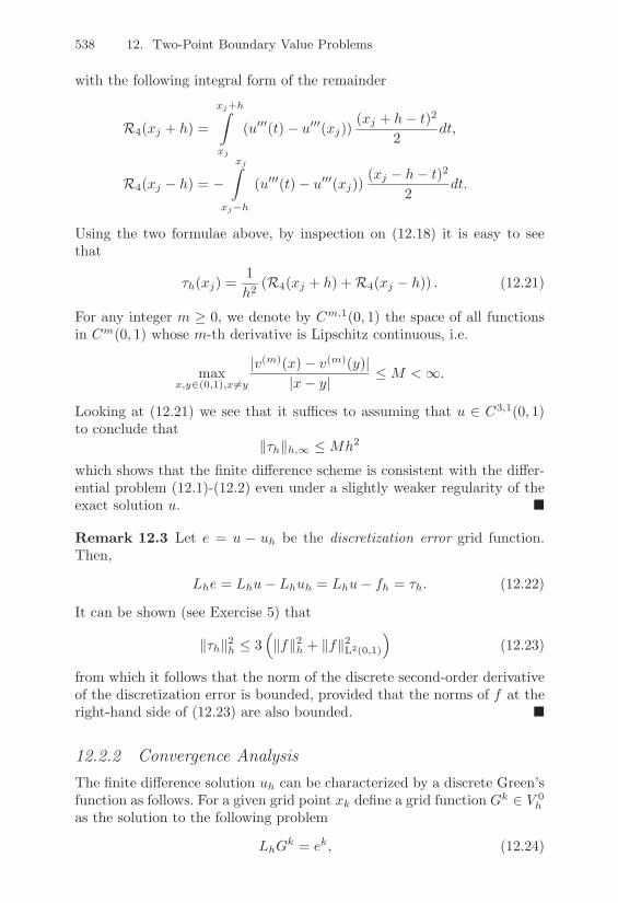
538 12. Two-Point Boundary Value Problems
with the following integral form of the remainder
R4(xj + h) =
xj+h^
xj
(u***(t)" u***(xj))(xj + h" t)2
2dt,
R4(xj " h) = "xj^
xj"h
(u***(t)" u***(xj))(xj " h" t)2
2dt.
Using the two formulae above, by inspection on (12.18) it is easy to seethat
5h(xj) =1h2 (R4(xj + h) + R4(xj " h)) . (12.21)
For any integer m ) 0, we denote by Cm,1(0, 1) the space of all functionsin Cm(0, 1) whose m-th derivative is Lipschitz continuous, i.e.
maxx,y#(0,1),x '=y
|v(m)(x)" v(m)(y)||x" y| &M <,.
Looking at (12.21) we see that it su"ces to assuming that u ! C3,1(0, 1)to conclude that
+5h+h,$ &Mh2
which shows that the finite di!erence scheme is consistent with the di!er-ential problem (12.1)-(12.2) even under a slightly weaker regularity of theexact solution u. !
Remark 12.3 Let e = u " uh be the discretization error grid function.Then,
Lhe = Lhu" Lhuh = Lhu" fh = 5h. (12.22)
It can be shown (see Exercise 5) that
+5h+2h & 3K+f+2h + +f+2L2(0,1)
L(12.23)
from which it follows that the norm of the discrete second-order derivativeof the discretization error is bounded, provided that the norms of f at theright-hand side of (12.23) are also bounded. !
12.2.2 Convergence AnalysisThe finite di!erence solution uh can be characterized by a discrete Green’sfunction as follows. For a given grid point xk define a grid function Gk ! V 0
has the solution to the following problem
LhGk = ek, (12.24)

12.2 Finite Di"erence Approximation 539
where ek ! V 0h satisfies ek(xj) = %kj , 1 & j & n " 1. It is easy to see
that Gk(xj) = hG(xj , xk), where G is the Green’s function introduced in(12.4) (see Exercise 6). For any grid function g ! V 0
h we can define the gridfunction
wh = Thg, wh =n"1(
k=1
g(xk)Gk. (12.25)
Then
Lhwh =n"1(
k=1
g(xk)LhGk =
n"1(
k=1
g(xk)ek = g.
In particular, the solution uh of (12.10) satisfies uh = Thf , therefore
uh =n"1(
k=1
f(xk)Gk, and uh(xj) = hn"1(
k=1
G(xj , xk)f(xk). (12.26)
Theorem 12.1 Assume that f ! C2([0, 1]). Then, the nodal error e(xj) =u(xj)" uh(xj) satisfies
+u" uh+h,$ & h2
96+f **+$, (12.27)
i.e. uh converges to u (in the discrete maximum norm) with second orderwith respect to h.
Proof. We start by noticing that, thanks to the representation (12.25), thefollowing discrete counterpart of (12.5) holds
&uh&h,! " 18&f&h,!. (12.28)
Indeed, we have
|uh(xj)| " hn%1(
k=1
G(xj , xk)|f(xk)| " &f&h,!
6
hn%1(
k=1
G(xj , xk)
7
= &f&h,!12xj(1% xj) "
18&f&h,!
since, if g = 1, then Thg is such that Thg(xj) = 12xj(1% xj) (see Exercise 7).
Inequality (12.28) provides a result of stability in the discrete maximum normfor the finite di"erence solution uh. Using (12.22), by the same argument used toprove (12.28) we obtain
&e&h,! " 18&4h&h,!.
Finally, the thesis (12.27) follows owing to (12.20). !
Observe that for the derivation of the convergence result (12.27) we haveused both stability and consistency. In particular, the discretization erroris of the same order (with respect to h) as the consistency error 5h.

540 12. Two-Point Boundary Value Problems
12.2.3 Finite Di!erences for Two-Point Boundary ValueProblems with Variable Coe"cients
A two-point boundary value problem more general than (12.1)-(12.2) is thefollowing one
Lu(x) = "(J(u)(x))* + '(x)u(x) = f(x) 0 < x < 1,
u(0) = d0, u(1) = d1
(12.29)
where
J(u)(x) = "(x)u*(x), (12.30)
d0 and d1 are assigned constants and ", ' and f are given functions thatare continuous in [0, 1]. Finally, '(x) ) 0 in [0, 1] and "(x) ) "0 > 0 for asuitable "0. The auxiliary variable J(u) is the flux associated with u andvery often has a precise physical meaning.
For the approximation, it is convenient to introduce on [0, 1] a new gridmade by the midpoints xj+1/2 = (xj + xj+1)/2 of the intervals [xj , xj+1]for j = 0, . . . , n " 1. Then, a finite di!erence approximation of (12.29) isgiven by: find uh ! Vh such that
Lhuh(xj) = f(xj) for all j = 1, . . . , n" 1,
uh(x0) = d0, uh(xn) = d1,(12.31)
where Lh is defined for j = 1, . . . , n" 1 as
Lhw(xj) = "Jj+1/2(wh)" Jj"1/2(wh)
h+ 'jwj . (12.32)
We have defined 'j = '(xj) and, for j = 0, . . . , n " 1, the approximatefluxes are given by
Jj+1/2(wh) = "j+1/2wj+1 " wj
h(12.33)
with "j+1/2 = "(xj+1/2).The finite di!erence scheme (12.31)-(12.32) with the approximate fluxes(12.33) can still be cast in the form (12.7) by setting
Afd = h"2tridiagn"1(a,d,a) + diagn"1(c) (12.34)
where
a =8"1/2,"3/2, . . . ,"n"1/2
9T ! Rn"2,
d =8"1/2 + "3/2, . . . ,"n"3/2 + "n"1/2
9T ! Rn"1,
c = ('1, . . . , 'n"1)T ! Rn"1.
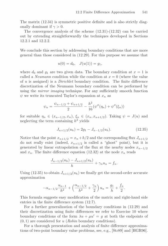
12.2 Finite Di"erence Approximation 541
The matrix (12.34) is symmetric positive definite and is also strictly diag-onally dominant if ' > 0.
The convergence analysis of the scheme (12.31)-(12.32) can be carriedout by extending straightforwardly the techniques developed in Sections12.2.1 and 12.2.2.
We conclude this section by addressing boundary conditions that are moregeneral than those considered in (12.29). For this purpose we assume that
u(0) = d0, J(u(1)) = g1,
where d0 and g1 are two given data. The boundary condition at x = 1 iscalled a Neumann condition while the condition at x = 0 (where the valueof u is assigned) is a Dirichlet boundary condition. The finite di!erencediscretization of the Neumann boundary condition can be performed byusing the mirror imaging technique. For any su"ciently smooth function6 we write its truncated Taylor’s expansion at xn as
6n =6n"1/2 + 6n+1/2
2" h2
16(6**(-n) + 6**(*n))
for suitable -n ! (xn"1/2, xn), *n ! (xn, xn+1/2). Taking 6 = J(u) andneglecting the term containing h2 yields
Jn+1/2(uh) = 2g1 " Jn"1/2(uh). (12.35)
Notice that the point xn+1/2 = xn+h/2 and the corresponding flux Jn+1/2do not really exist (indeed, xn+1/2 is called a “ghost” point), but it isgenerated by linear extrapolation of the flux at the nearby nodes xn"1/2and xn. The finite di!erence equation (12.32) at the node xn reads
Jn"1/2(uh)" Jn+1/2(uh)h
+ 'nun = fn.
Using (12.35) to obtain Jn+1/2(uh) we finally get the second-order accurateapproximation
""n"1/2un"1
h2 +K"n"1/2
h2 +'n2
Lun =
g1
h+
fn2.
This formula suggests easy modification of the matrix and right-hand sideentries in the finite di!erence system (12.7).
For a further generalization of the boundary conditions in (12.29) andtheir discretization using finite di!erences we refer to Exercise 10 whereboundary conditions of the form $u + µu* = g at both the endpoints of(0, 1) are considered for u (Robin boundary conditions).
For a thorough presentation and analysis of finite di!erence approxima-tions of two-point boundary value problems, see, e.g., [Str89] and [HGR96].

542 12. Two-Point Boundary Value Problems
12.3 The Spectral Collocation Method
Other discretization schemes can be derived which exhibit the same struc-ture as the finite di!erence problem (12.10), with a discrete operator Lh
being defined in a di!erent manner, though.Actually, numerical approximations of the second derivative other than
the centred finite di!erence one can be set up, as described in Section10.10.3. A noticeable instance is provided by the spectral collocation method.In that case we assume the di!erential equation (12.1) to be set on the in-terval ("1, 1) and choose the nodes {x0, . . . , xn} to coincide with the n+1Legendre-Gauss-Lobatto nodes introduced in Section 10.4. Besides, uh is apolynomial of degree n. For coherence, we will use throughout the sectionthe index n instead of h.
The spectral collocation problem reads
find un ! P0n : Lnun(xj) = f(xj), j = 1, . . . , n" 1 (12.36)
where P0n is the set of polynomials p ! Pn([0, 1]) such that p(0) = p(1) = 0.
Besides, Lnv = LInv for any continuous function v where Inv ! Pn is theinterpolant of v at the nodes {x0, . . . , xn} and L denotes the di!erentialoperator at hand, which, in the case of equation (12.1), coincides with"d2/dx2. Clearly, if v ! Pn then Lnv = Lv.
The algebraic form of (12.36) becomes
Aspu = f ,
where uj = un(xj), fj = f(xj) j = 1, . . . , n"1 and the spectral collocationmatrix Asp ! R(n"1)!(n"1) is equal to D2, where D is the matrix obtainedfrom the pseudo-spectral di!erentiation matrix (10.73) by eliminating thefirst and the n + 1-th rows and columns.
For the analysis of (12.36) we can introduce the following discrete scalarproduct
(u, v)n =n(
j=0
u(xj)v(xj)wj , (12.37)
where wj are the weights of the Legendre-Gauss-Lobatto quadrature for-mula (see Section 10.4). Then (12.36) is equivalent to
(Lnun, vn)n = (f, vn)n #vn ! P0n. (12.38)
Since (12.37) is exact for u, v such that uv ! P2n"1 (see Section 10.2) then
(Lnvn, vn)n = (Lnvn, vn) = +v*n+2L2("1,1), #vn ! P0n.
Besides,
(f, vn)n & +f+n+vn+n &/
6+f+$ +vn+L2("1,1),

12.3 The Spectral Collocation Method 543
where +f+$ denotes the maximum of f in ["1, 1] and we have used thefact that +f+n &
/2+f+$ and the result of equivalence
+vn+L2("1,1) & +vn+n &/
3+vn+L2("1,1), #vn ! Pn
(see [CHQZ88], p. 286).Taking vn = un in (12.38) and using the Poincare inequality (12.16) we
finally obtain
+u*n+L2("1,1) &
/6CP +f+$
which ensures that problem (12.36) has a unique solution which is stable.As for consistency, we can notice that
5n(xj) = (Lnu" f)(xj) = ("(Inu)** " f)(xj) = (u" Inu)**(xj)
and this right-hand side tends to zero as n ( , provided that u !C2(["1, 1]).
Let us now establish a convergence result for the spectral collocationapproximation of (12.1). In the following, C is a constant independent ofn that can assume di!erent values at di!erent places.
Moreover, we denote by Hs(a, b), for s ) 1, the space of the functions f !Cs"1(a, b) such that f (s"1) is continuous and piecewise di!erentiable, sothat f (s) exists unless for a finite number of points and belongs to L2(a, b).The space Hs(a, b) is known as the Sobolev function space of order s and isendowed with the norm + · +Hs(a,b) defined in (10.35).
Theorem 12.2 Let f ! Hs("1, 1) for some s ) 1. Then
+u* " u*n+L2("1,1) & Cn"s
8+f+Hs("1,1) + +u+Hs+1("1,1)
9. (12.39)
Proof. Note that un satisfies
(u(n, v
(n) = (f, vn)n
where (u, v) =@ 1%1 uvdx is the scalar product of L2(%1, 1). Similarly, u satisfies
(u(, v() = (f, v) )v / C1([0, 1]) such that v(0) = v(1) = 0
(see (12.43) of Section 12.4). Then
((u% un)(, v(n) = (f, vn)% (f, vn)n =: E(f, vn), )vn / P0n.
It follows that
((u% un)(, (u% un)() = ((u% un)(, (u% Inu)() + ((u% un)(, (Inu% un)()
= ((u% un)(, (u% Inu)() + E(f, Inu% un).
We recall the following result (see (10.36))
|E(f, vn)| " Cn%s&f&Hs(%1,1)&vn&L2(%1,1).

544 12. Two-Point Boundary Value Problems
Then
|E(f, Inu% un)| " Cn%s&f&Hs(%1,1)8&Inu% u&L2(%1,1) + &u% un&L2(%1,1)
9.
We recall now the following Young’s inequality (see Exercise 8)
ab " &a2 +14&
b2, )a, b / R, )& > 0. (12.40)
Using this inequality we obtain
8(u% un)(, (u% Inu)(
9" 1
4&(u% un)(&2L2(%1,1) + &(u% Inu)(&2L2(%1,1),
and also (using the Poincare inequality (12.16))
Cn%s&f&Hs(%1,1)&u% un&L2(%1,1) " C CP n%s&f&Hs(%1,1)&(u% un)(&L2(%1,1)
" (CCP )2n%2s&f&2Hs(%1,1) +14&(u% un)(&2L2(%1,1).
Finally,
Cn%s&f&Hs(%1,1)&Inu% u&L2(%1,1) "12C2n%2s&f&2Hs(%1,1) +
12&Inu% u&2L2(%1,1).
Using the interpolation error estimate (10.22) for u % Inu we finally obtain thedesired error estimate (12.39). !
12.4 The Galerkin Method
We now derive the Galerkin approximation of problem (12.1)-(12.2), whichis the basic ingredient of the finite element method and the spectral method,widely employed in the numerical approximation of boundary value prob-lems.
12.4.1 Integral Formulation of Boundary Value ProblemsWe consider a problem which is slightly more general than (12.1), namely
"("u*)*(x) + (#u*)(x) + ('u)(x) = f(x) 0 < x < 1, (12.41)
with u(0) = u(1) = 0, where ", # and ' are continuous functions on [0, 1]with "(x) ) "0 > 0 for any x ! [0, 1]. Let us now multiply (12.41) bya function v ! C1([0, 1]), hereafter called a “test function”, and integrateover the interval [0, 1]
1^
0
"u*v* dx +1^
0
#u*v dx +1^
0
'uv dx =1^
0
fv dx + ["u*v]10,

12.4 The Galerkin Method 545
where we have used integration by parts on the first integral. If the functionv is required to vanish at x = 0 and x = 1 we obtain
1^
0
"u*v* dx +1^
0
#u*v dx +1^
0
'uv dx =1^
0
fv dx.
We will denote by V the test function space. This consists of all functions vthat are continuous, vanish at x = 0 and x = 1 and whose first derivative ispiecewise continuous, i.e., continuous everywhere except at a finite numberof points in [0, 1] where the left and right limits v*" and v*+ exist but do notnecessarily coincide.
V is actually a vector space which is denoted by H10(0, 1). Precisely,
H10(0, 1) =
/v ! L2(0, 1) : v* ! L2(0, 1), v(0) = v(1) = 0
0(12.42)
where v* is the distributional derivative of v whose definition is given inSection 12.4.2.
We have therefore shown that if a function u ! C2([0, 1]) satisfies (12.41),then u is also a solution of the following problem
find u ! V : a(u, v) = (f, v) for all v ! V, (12.43)
where now (f, v) =@ 10 fv dx denotes the scalar product of L2(0, 1) and
a(u, v) =1^
0
"u*v* dx +1^
0
#u*v dx +1^
0
'uv dx (12.44)
is a bilinear form, i.e. it is linear with respect to both arguments u andv. Problem (12.43) is called the weak formulation of problem (12.1). Since(12.43) contains only the first derivative of u it might cover cases in whicha classical solution u ! C2([0, 1]) of (12.41) does not exist although thephysical problem is well defined.
If for instance, " = 1, # = ' = 0, the solution u(x) denotes of thedisplacement at point x of an elastic cord having linear density equal to f ,whose position at rest is u(x) = 0 for all x ! [0, 1] and which remains fixedat the endpoints x = 0 and x = 1. Figure 12.2 (right) shows the solutionu(x) corresponding to a function f which is discontinuous (see Figure 12.2,left). Clearly, u** does not exist at the points x = 0.4 and x = 0.6 where fis discontinuous.
If (12.41) is supplied with non homogeneous boundary conditions, sayu(0) = u0, u(1) = u1, we can still obtain a formulation like (12.43) byproceeding as follows. Let u(x) = xu1 + (1" x)u0 be the straight line thatinterpolates the data at the endpoints, and set
0u= u(x)" u(x). Then
0u! V

546 12. Two-Point Boundary Value Problems
10.60.40
!1
f(x)
x
0 0.1 0.2 0.3 0.4 0.5 0.6 0.7 0.8 0.9 1!0.05
!0.045
!0.04
!0.035
!0.03
!0.025
!0.02
!0.015
!0.01
!0.005
0
u(x)
FIGURE 12.2. Elastic cord fixed at the endpoints and subject to a discontinuousload f (left). The vertical displacement u is shown on the right
satisfies the following problem
find0u! V : a(
0u, v) = (f, v)" a(u, v) for all v ! V.
A similar problem is obtained in the case of Neumann boundary conditions,say u*(0) = u*(1) = 0. Proceeding as we did to obtain (12.43), we seethat the solution u of this homogeneous Neumann problem satisfies thesame problem (12.43) provided the space V is now H1(0, 1). More generalboundary conditions of mixed type can be considered as well (see Exercise12).
12.4.2 A Quick Introduction to DistributionsLet X be a Banach space, i.e., a normed and complete vector space. Wesay that a functional T : X ( R is continuous if limx&x0 T (x) = T (x0)for all x0 ! X and linear if T (x + y) = T (x) + T (y) for any x, y ! X andT ($x) = $T (x) for any x ! X and $ ! R.
Usually, a linear continuous functional is denoted by BT, xC and the sym-bol B·, ·C is called duality. As an example, let X = C0([0, 1]) be endowedwith the maximum norm + · +$ and consider on X the two functionalsdefined as
BT, xC = x(0), BS, xC =^ 1
0x(t) sin(t)dt.
It is easy to check that both T and S are linear and continuous functionalson X. The set of all linear continuous functionals on X identifies an abstractspace which is called the dual space of X and is denoted by X *.
We then introduce the space C$0 (0, 1) (or D(0, 1)) of infinitely di!er-
entiable functions having compact support in [0, 1], i.e., vanishing outsidea bounded open set (a, b) * (0, 1) with 0 < a < b < 1. We say thatvn ! D(0, 1) converges to v ! D(0, 1) if there exists a closed bounded setK * (0, 1) such that vn vanishes outside K for each n and for any k ) 0the derivative v(k)
n converges to v(k) uniformly in (0, 1).

12.4 The Galerkin Method 547
The space of linear functionals on D(0, 1) which are continuous withrespect to the convergence introduced above is denoted by D*(0, 1) (thedual space of D(0, 1)) and its elements are called distributions.
We are now in position to introduce the derivative of a distribution. LetT be a distribution, i.e. an element of D*(0, 1). Then, for any k ) 0, T (k)
is also a distribution, defined as
BT (k),1C = ("1)kBT,1(k)C, #1 ! D(0, 1). (12.45)
As an example, consider the Heaviside function
H(x) =
B1 x ) 0,
0 x < 0.
The distributional derivative of H is the Dirac mass % at the origin, definedas
v ( %(v) = v(0), v ! D(R).
From the definition (12.45), it turns out that any distribution is infinitelydi!erentiable; moreover, if T is a di!erentiable function its distributionalderivative coincides with the usual one.
12.4.3 Formulation and Properties of the Galerkin MethodUnlike the finite di!erence method which stems directly from the di!er-ential (or strong) form (12.41), the Galerkin method is based on the weakformulation (12.43). If Vh is a finite dimensional vector subspace of V , theGalerkin method consists of approximating (12.43) by the problem
find uh ! Vh : a(uh, vh) = (f, vh) #vh ! Vh. (12.46)
This is a finite dimensional problem. Actually, let {11, . . . ,1N} denote abasis of Vh, i.e. a set of N linearly independent functions of Vh. Then wecan write
uh(x) =N(
j=1
uj1j(x).
The integer N denotes the dimension of the vector space Vh. Taking vh = 1i
in (12.46), it turns out that the Galerkin problem (12.46) is equivalent toseeking N unknown coe"cients {u1, . . . , uN} such that
N(
j=1
uja(1j ,1i) = (f,1i) #i = 1, . . . , N. (12.47)

548 12. Two-Point Boundary Value Problems
We have used the linearity of a(·, ·) with respect to its first argument, i.e.
a(N(
j=1
uj1j ,1i) =N(
j=1
uja(1j ,1i).
If we introduce the matrix AG = (aij), aij = a(1j ,1i) (called the sti!nessmatrix), the unknown vector u = (u1, . . . , uN ) and the right-hand sidevector fG = (f1, . . . , fN ), with fi = (f,1i), we see that (12.47) is equivalentto the linear system
AGu = fG. (12.48)
The structure of AG, as well as the degree of accuracy of uh, depends onthe form of the basis functions {1i}, and therefore on the choice of Vh.
We will see two remarkable instances, the finite element method, whereVh is a space of piecewise polynomials over subintervals of [0, 1] of length notgreater than h which are continuous and vanish at the endpoints x = 0 and1, and the spectral method in which Vh is a space of algebraic polynomialsstill vanishing at the endpoints x = 0, 1.
However, before specifically addressing those cases, we state a couple ofgeneral results that hold for any Galerkin problem (12.46).
12.4.4 Analysis of the Galerkin MethodWe endow the space H1
0(0, 1) with the following norm
|v|H1(0,1) =
)+
,
1^
0
|v*(x)|2 dx
_`
a
1/2
. (12.49)
We will address the special case where # = 0 and '(x) ) 0. In the mostgeneral case given by the di!erential problem (12.41) we shall assume thatthe coe"cients satisfy
"12#* + ' ) 0, #x ! [0, 1]. (12.50)
This ensures that the Galerkin problem (12.46) admits a unique solutiondepending continuously on the data. Taking vh = uh in (12.46) we obtain
"0|uh|2H1(0,1) &1^
0
"u*hu
*h dx +
1^
0
'uhuh dx = (f, uh) & +f+L2(0,1)+uh+L2(0,1),
where we have used the Cauchy-Schwarz inequality (8.29) to set the right-hand side inequality. Owing to the Poincare inequality (12.16) we concludethat
|uh|H1(0,1) &CP
"0+f+L2(0,1). (12.51)

12.4 The Galerkin Method 549
Thus, the norm of the Galerkin solution remains bounded (uniformly withrespect to the dimension of the subspace Vh) provided that f ! L2(0, 1).Inequality (12.51) therefore represents a stability result for the solution ofthe Galerkin problem.
As for convergence, we can prove the following result.
Theorem 12.3 Let C = ""10 (+"+$ + C2
P +'+$); then, we have
|u" uh|H1(0,1) & C minwh#Vh
|u" wh|H1(0,1). (12.52)
Proof. Subtracting (12.46) from (12.43) (where we use vh / Vh 5 V ), owing tothe bilinearity of the form a(·, ·) we obtain
a(u% uh, vh) = 0 )vh / Vh. (12.53)
Then, setting e(x) = u(x)% uh(x), we deduce
$0|e|2H1(0,1) " a(e, e) = a(e, u% wh) + a(e, wh % uh) )wh / Vh.
The last term is null due to (12.53). On the other hand, still by the Cauchy-Schwarz inequality we obtain
a(e, u% wh) =1^
0
$e((u% wh)( dx +1^
0
,e(u% wh) dx
" &$&!|e|H1(0,1)|u% wh|H1(0,1) + &,&!&e&L2(0,1)&u% wh&L2(0,1).
The desired result (12.52) now follows by using again the Poincare inequality forboth &e&L2(0,1) and &u% wh&L2(0,1). !
The previous results can be obtained under more general hypotheses onproblems (12.43) and (12.46). Precisely, we can assume that V is a Hilbertspace, endowed with norm + ·+V , and that the bilinear form a : V %V ( R
satisfies the following properties:
-"0 > 0 : a(v, v) ) "0+v+2V #v ! V (coercivity), (12.54)
-M > 0 : |a(u, v)| &M+u+V +v+V #u, v ! V (continuity). (12.55)
Moreover, the right hand side (f, v) satisfies the following inequality
|(f, v)| & K+v+V #v ! V.
Then both problems (12.43) and (12.46) admit unique solutions that satisfy
+u+V &K
"0, +uh+V &
K
"0.

550 12. Two-Point Boundary Value Problems
This is a celebrated result which is known as the Lax-Milgram Lemma (forits proof see, e.g., [QV94]). Besides, the following error inequality holds
+u" uh+V &M
"0min
wh#Vh
+u" wh+V . (12.56)
The proof of this last result, which is known as Cea’s Lemma, is very similarto that of (12.52) and is left to the reader.
We now wish to notice that, under the assumption (12.54), the matrixintroduced in (12.48) is positive definite. To show this, we must check thatvTBv ) 0 #v ! RN and that vTBv = 0 . v = 0 (see Section 1.12).
Let us associate with a generic vector v = (vi) of RN the function vh =!Nj=1 vj1j ! Vh. Since the form a(·, ·) is bilinear and coercive we get
vTAGv =N(
j=1
N(
i=1
viaijvj =N(
j=1
N(
i=1
via(1j ,1i)vj
=N(
j=1
N(
i=1
a(vj1j , vi1i) = a
G
HN(
j=1
vj1j ,N(
i=1
vi1i
I
J
= a(vh, vh) ) "+vh+2V ) 0.
Moreover, if vTAGv = 0 then also +vh+2V = 0 which implies vh = 0 andthus v = 0.
It is also easy to check that the matrix AG is symmetric i! the bilinearform a(·, ·) is symmetric.
For example, in the case of problem (12.41) with # = ' = 0 the ma-trix AG is symmetric and positive definite (s.p.d.) while if # and ' arenonvanishing, AG is positive definite only under the assumption (12.50).If AG is s.p.d. the numerical solution of the linear system (12.48) can bee"ciently carried out using direct methods like the Cholesky factorization(see Section 3.4.2) as well as iterative methods like the conjugate gradientmethod (see Section 4.3.4). This is of particular interest in the solution ofboundary value problems in more than one space dimension (see Section12.6).
12.4.5 The Finite Element MethodThe finite element method (FEM) is a special technique for constructinga subspace Vh in (12.46) based on the piecewise polynomial interpolationconsidered in Section 8.3. With this aim, we introduce a partition Th of[0,1] into n subintervals Ij = [xj , xj+1], n ) 2, of width hj = xj+1 " xj ,j = 0, . . . , n" 1, with
0 = x0 < x1 < . . . < xn"1 < xn = 1

12.4 The Galerkin Method 551
and let h = maxTh
(hj). Since functions in H10(0, 1) are continuous it makes
sense to consider for k ) 1 the family of piecewise polynomials Xkh intro-
duced in (8.22) (where now [a, b] must be replaced by [0, 1]). Any functionvh ! Xk
h is a continuous piecewise polynomial over [0, 1] and its restrictionover each interval Ij ! Th is a polynomial of degree & k. In the followingwe shall mainly deal with the cases k = 1 and k = 2.
Then, we set
Vh = Xk,0h =
/vh ! Xk
h : vh(0) = vh(1) = 00. (12.57)
The dimension N of the finite element space Vh is equal to nk " 1. In thefollowing the two cases k = 1 and k = 2 will be examined.
To assess the accuracy of the Galerkin FEM we first notice that, thanksto Cea’s lemma (12.56), we have
minwh#Vh
+u" wh+H10(0,1) & +u"$
khu+H1
0(0,1) (12.58)
where $khu is the interpolant of the exact solution u ! V of (12.43) (see
Section 8.3). From inequality (12.58) we conclude that the matter of esti-mating the Galerkin approximation error +u"uh+H1
0(0,1) is turned into theestimate of the interpolation error +u " $k
hu+H10(0,1). When k = 1, using
(12.56) and (8.27) we obtain
+u" uh+H10(0,1) &
M
"0Ch+u+H2(0,1)
provided that u ! H2(0, 1). This estimate can be extended to the case k > 1as stated in the following convergence result (for its proof we refer, e.g., to[QV94], Theorem 6.2.1).
Property 12.1 Let u ! H10(0, 1) be the exact solution of (12.43) and uh !
Vh its finite element approximation using continuous piecewise polynomialsof degree k ) 1. Assume also that u ! Hs(0, 1) for some s ) 2. Then thefollowing error estimate holds
+u" uh+H10(0,1) &
M
"0Chl+u+Hl+1(0,1) (12.59)
where l = min(k, s " 1). Under the same assumptions, one can also provethat
+u" uh+L2(0,1) & Chl+1+u+Hl+1(0,1). (12.60)
The estimate (12.59) shows that the Galerkin method is convergent, i.e. theapproximation error tends to zero as h( 0 and the order of convergence is

552 12. Two-Point Boundary Value Problems
k. We also see that there is no convenience in increasing the degree k of thefinite element approximation if the solution u is not su"ciently smooth. Inthis respect l is called a regularity threshold. The obvious alternative to gainaccuracy in such a case is to reduce the stepzise h. Spectral methods, whichwill be considered in Section 12.4.7, instead pursue the opposite strategy(i.e. increasing the degree k) and are thus ideally suited to approximatingproblems with highly smooth solutions.
An interesting situation is that where the exact solution u has the min-imum regularity (s = 1). In such a case, Cea’s lemma ensures that theGalerkin FEM is still convergent since as h( 0 the subspace Vh becomesdense into V . However, the estimate (12.59) is no longer valid so thatit is not possible to establish the order of convergence of the numericalmethod. Table 12.1 summarizes the orders of convergence of the FEM fork = 1, . . . , 4 and s = 1, . . . , 5.
k s = 1 s = 2 s = 3 s = 4 s = 5
1 only convergence h1 h1 h1 h1
2 only convergence h1 h2 h2 h2
3 only convergence h1 h2 h3 h3
4 only convergence h1 h2 h3 h4
TABLE 12.1. Order of convergence of the FEM as a function of k (the degree ofinterpolation) and s (the Sobolev regularity of the solution u)
Let us now focus on how to generate a suitable basis {1j} for the finiteelement space Xk
h in the special cases k = 1 and k = 2. The basic point isto choose appropriately a set of degrees of freedom for each element Ij ofthe partition Th (i.e., the parameters which permit uniquely identifying afunction in Xk
h). The generic function vh in Xkh can therefore be written as
vh(x) =nk(
i=0
vi1i(x)
where {vi} denote the set of the degrees of freedom of vh and the basisfunctions 1i (which are also called shape functions) are assumed to satisfythe Lagrange interpolation property 1i(xj) = %ij , i, j = 0, . . . , n, where %ijis the Kronecker symbol.
The space X1h
This space consists of all continuous and piecewise linear functions overthe partition Th. Since a unique straight line passes through two distinctnodes the number of degrees of freedom for vh is equal to the numbern + 1 of nodes in the partition. As a consequence, n + 1 shape functions

12.4 The Galerkin Method 553
1i, i = 0, . . . , n, are needed to completely span the space X1h. The most
natural choice for 1i, i = 1, . . . , n" 1, is
1i(x) =
)******+
******,
x" xi"1
xi " xi"1for xi"1 & x & xi,
xi+1 " x
xi+1 " xifor xi & x & xi+1,
0 elsewhere.
(12.61)
The shape function 1i is thus piecewise linear over Th, its value is 1 atthe node xi and 0 at all the other nodes of the partition. Its support (i.e.,the subset of [0, 1] where 1i is nonvanishing) consists of the union of theintervals Ii"1 and Ii if 1 & i & n" 1 while it coincides with the interval I0(respectively In"1) if i = 0 (resp., i = n). The plots of 1i, 10 and 1n areshown in Figure 12.3.
1
x1x0 xi!1 xi xi+1 xn!1 xn = 1
"i "n"0
FIGURE 12.3. Shape functions of X1h associated with internal and boundary
nodes
For any interval Ii = [xi, xi+1], i = 0, . . . , n" 1, the two basis functions 1i
and 1i+1 can be regarded as the images of two “reference” shape functions:10 and :11 (defined over the reference interval [0, 1]) through the lineara"ne mapping 4 : [0, 1] ( Ii
x = 4(*) = xi + *(xi+1 " xi), i = 0, . . . , n" 1. (12.62)
Defining :10(*) = 1 " *, :11(*) = *, the two shape functions 1i and 1i+1can be constructed over the interval Ii as
1i(x) = :10(*(x)), 1i+1(x) = :11(*(x))
where *(x) = (x" xi)/(xi+1 " xi) (see Figure 12.4).

554 12. Two-Point Boundary Value Problems
0 1
:11
*
1
xi xi+1
1i+1
x
1""(
FIGURE 12.4. Linear a!ne mapping 3 from the reference interval to the genericinterval of the partition
The space X2h
The generic function vh ! X2h is a piecewise polynomial of degree 2 over
each interval Ii. As such, it can be uniquely determined once three valuesof it at three distinct points of Ii are assigned. To ensure continuity ofvh over [0, 1] the degrees of freedom are chosen as the function values atthe nodes xi of Th, i = 0, . . . , n, and at the midpoints of each interval Ii,i = 0, . . . , n " 1, for a total number equal to 2n + 1. It is convenient tolabel the degrees of freedom and the corresponding nodes in the partitionstarting from x0 = 0 until x2n = 1 in such a way that the midpoints ofeach interval correspond to the nodes with odd index while the endpointsof each interval correspond to the nodes with even index.
The explicit expression of the single shape function is
(i even) 1i(x) =
)******+
******,
(x" xi"1)(x" xi"2)(xi " xi"1)(xi " xi"2)
for xi"2 & x & xi,
(xi+1 " x)(xi+2 " x)(xi+1 " xi)(xi+2 " xi)
for xi & x & xi+2,
0 elsewhere,
(12.63)
(i odd) 1i(x) =
)*+
*,
(xi+1 " x)(x" xi"1)(xi+1 " xi)(xi " xi"1)
for xi"1 & x & xi+1,
0 elsewhere.(12.64)
Each basis function enjoys the property that 1(xj) = %ij , i, j = 0, . . . , 2n.The shape functions for X2
h on the reference interval [0, 1] are
:10(*) = (1" *)(1" 2*), :11(*) = 4(1" *)*, :12(*) = *(2* " 1)(12.65)
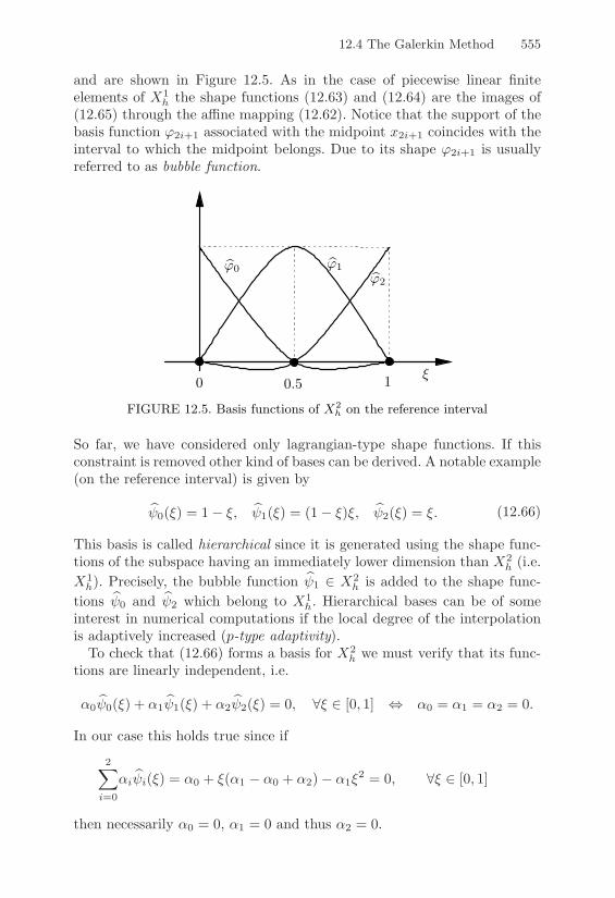
12.4 The Galerkin Method 555
and are shown in Figure 12.5. As in the case of piecewise linear finiteelements of X1
h the shape functions (12.63) and (12.64) are the images of(12.65) through the a"ne mapping (12.62). Notice that the support of thebasis function 12i+1 associated with the midpoint x2i+1 coincides with theinterval to which the midpoint belongs. Due to its shape 12i+1 is usuallyreferred to as bubble function.
:12
:11:10
*0 0.5 1
FIGURE 12.5. Basis functions of X2h on the reference interval
So far, we have considered only lagrangian-type shape functions. If thisconstraint is removed other kind of bases can be derived. A notable example(on the reference interval) is given by
:60(*) = 1" *, :61(*) = (1" *)*, :62(*) = *. (12.66)
This basis is called hierarchical since it is generated using the shape func-tions of the subspace having an immediately lower dimension than X2
h (i.e.X1
h). Precisely, the bubble function :61 ! X2h is added to the shape func-
tions :60 and :62 which belong to X1h. Hierarchical bases can be of some
interest in numerical computations if the local degree of the interpolationis adaptively increased (p-type adaptivity).
To check that (12.66) forms a basis for X2h we must verify that its func-
tions are linearly independent, i.e.
"0 :60(*) + "1 :61(*) + "2 :62(*) = 0, #* ! [0, 1] . "0 = "1 = "2 = 0.
In our case this holds true since if
2(
i=0
"i:6i(*) = "0 + *("1 " "0 + "2)" "1*
2 = 0, #* ! [0, 1]
then necessarily "0 = 0, "1 = 0 and thus "2 = 0.

556 12. Two-Point Boundary Value Problems
A procedure analogous to that examined in the sections above can be usedin principle to construct a basis for every subspace Xk
h with k being arbi-trary. However, it is important to remember that an increase in the degree kof the polynomial approximation gives rise to an increase of the number ofdegrees of freedom of the FEM and, as a consequence, of the computationalcost required for the solution of the linear system (12.48).
Let us now examine the structure and the basic properties of the sti!nessmatrix associated with system (12.48) in the case of the finite elementmethod (AG = Afe).
Since the finite element basis functions for Xkh have a local support, Afe is
sparse. In the particular case k = 1, the support of the shape function 1i isthe union of the intervals Ii"1 and Ii if 1 & i & n"1, and it coincides withthe interval I0 (respectively In"1) if i = 0 (resp., i = n). As a consequence,for a fixed i = 1, . . . , n" 1, only the shape functions 1i"1 and 1i+1 have anonvanishing support intersection with that of 1i, which implies that Afeis tridiagonal since aij = 0 if j '! {i" 1, i, i + 1}. In the case k = 2 oneconcludes with an analogous argument that Afe is a pentadiagonal matrix.
The condition number of Afe is a function of the grid size h; indeed,
K2(Afe) = +Afe+2+A"1fe +2 = O(h"2)
(for the proof, see [QV94], Section 6.3.2), which demonstrates that theconditioning of the finite element system (12.48) grows rapidly as h (0. This is clearly conflicting with the need of increasing the accuracy ofthe approximation and, in multidimensional problems, demands suitablepreconditioning techniques if iterative solvers are used (see Section 4.3.2).
Remark 12.4 (Elliptic problems of higher order) The Galerkin me-thod in general, and the finite element method in particular, can also beapplied to other type of elliptic equations, for instance to those of fourthorder. In that case, the numerical solution (as well as the test functions)should be continuous together with their first derivative. An example hasbeen illustrated in Section 8.8.1. !
12.4.6 Implementation IssuesIn this section we implement the finite element (FE) approximation withpiecewise linear elements (k = 1) of the boundary value problem (12.41)(shortly, BVP) with non homogeneous Dirichlet boundary conditions.Here is the list of the input parameters of Program 94: Nx is the numberof grid subintervals; I is the interval [a, b], alpha, beta, gamma and f arethe macros corresponding to the coe"cients in the equation, bc=[ua,ub]is a vector containing the Dirichlet boundary conditions for u at x = a andx = b and stabfun is an optional string variable. It can assume di!erent

12.4 The Galerkin Method 557
values, allowing the user to select the desired type of artificial viscosity thatmay be needed for dealing with the problems addressed in Section 12.5.
Program 94 - ellfem : Linear FE for two-point BVPs
function [uh,x] = ellfem(Nx,I,alpha,beta,gamma,f,bc,stabfun)a = I(1); b = I(2); h = (b-a)/Nx; x = [a+h/2:h:b-h/2];alpha = eval(alpha); beta = eval(beta); gamma = eval(gamma);f = eval(f); rhs = 0.5*h*(f(1:Nx-1)+f(2:Nx));if nargin == 8[Afe,rhsbc] = femmatr(Nx,h,alpha,beta,gamma,stabfun);
else[Afe,rhsbc] = femmatr(Nx,h,alpha,beta,gamma);
end[L,U,P] = lu(Afe);rhs(1) = rhs(1)-bc(1)*(-alpha(1)/h-beta(1)/2+h*gamma(1)/3+rhsbc(1));rhs(Nx-1) = rhs(Nx-1)-bc(2)*(-alpha(Nx)/h+beta(Nx)/2+h*gamma(Nx)/3+rhsbc(2));rhs = P*rhs’; z = L \ rhs;w = U \ z;uh = [bc(1), w’, bc(2)]; x = [a:h:b];
Program 95 computes the sti!ness matrix Afe; with this aim, the coe"cients", # and ' and the forcing term f are replaced by piecewise constantfunctions on each mesh subinterval and the remaining integrals in (12.41),involving the basis functions and their derivatives, are evaluated exactly.
Program 95 - femmatr : Construction of the sti!ness matrix
function [Afe,rhsbc] = femmatr(Nx,h,alpha,beta,gamma,stabfun)for i=2:Nx
dd(i-1)=(alpha(i-1)+alpha(i))/h; dc(i-1)=-(beta(i)-beta(i-1))/2;dr(i-1)=h*(gamma(i-1)+gamma(i))/3;if i > 2ld(i-2) = -alpha(i-1)/h; lc(i-2)=-beta(i-1)/2;lr(i-2) = h*gamma(i-1)/6;
endif i < Nxud(i-1) = -alpha(i)/h; uc(i-1)=beta(i)/2;ur(i-1) = h*gamma(i)/6;
endendKd=spdiags([[ld 0]’,dd’,[0 ud]’],-1:1,Nx-1,Nx-1);Kc=spdiags([[lc 0]’,dc’,[0 uc]’],-1:1,Nx-1,Nx-1);Kr=spdiags([[lr 0]’,dr’,[0 ur]’],-1:1,Nx-1,Nx-1);Afe=Kd+Kc+Kr;if nargin == 6s=[’[Ks,rhsbc]=’,stabfun,’(Nx,h,alpha,beta);’]; eval(s)Afe = Afe + Ks;
else

558 12. Two-Point Boundary Value Problems
rhsbc = [0, 0];end
The H1-norm of the error can be computed by calling Program 96, whichmust be supplied by the macros u and ux containing the expression of theexact solution u and of u*. The computed numerical solution is stored inthe output vector uh, while the vector coord contains the grid coordinatesand h is the mesh size. The integrals involved in the computation of theH1-norm of the error are evaluated using the composite Simpson formula(9.17).
Program 96 - H1error : Computation of the H1-norm of the error
function [L2err,H1err]=H1error(coord,h,uh,u,udx)nvert=max(size(coord)); x=[]; k=0;for i = 1:nvert-1
xm = (coord(i+1)+coord(i))*0.5;x = [x, coord(i),xm]; k = k + 2;
endndof = k+1; x (ndof) = coord (nvert);uq = eval(u); uxq = eval(udx); L2err = 0; H1err = 0;for i=1:nvert-1
L2err = L2err + (h/6)*((uh(i)-uq(2*i-1))ˆ2+...4*(0.5*uh(i)+0.5*uh(i+1)-uq(2*i))ˆ2+(uh(i+1)-uq(2*i+1))ˆ2);
H1err = H1err + (1/(6*h))*((uh(i+1)-uh(i)-h*uxq(2*i-1))ˆ2+...4*(uh(i+1)-uh(i)-h*uxq(2*i))ˆ2+(uh(i+1)-uh(i)-h*uxq(2*i+1))ˆ2);
endH1err = sqrt(H1err + L2err); L2err = sqrt(L2err);
Example 12.1 We assess the accuracy of the finite element solution of the fol-lowing problem. Consider a thin rod of length L whose temperature at x = 0 isfixed to t0 while the other endpoint x = L is thermally isolated. Assume that therod has a cross-section with constant area equal to A and that the perimeter ofA is p.
The temperature u of the rod at a generic point x / (0, L) is governed by thefollowing boundary value problem with mixed Dirichlet-Neumann conditions
)+
,
%µAu(( + 'pu = 0 x / (0, L),
u(0) = u0, u((L) = 0,(12.67)
where µ denotes the thermal conductivity and ' is the convective transfer coef-ficient. The exact solution of the problem is the (smooth) function
u(x) = u0cosh[m(L% x)]
cosh(mL),
where m =3
'p/µA. We solve the problem by using linear and quadratic finiteelements (k = 1 and k = 2) on a grid with uniform size. In the numerical
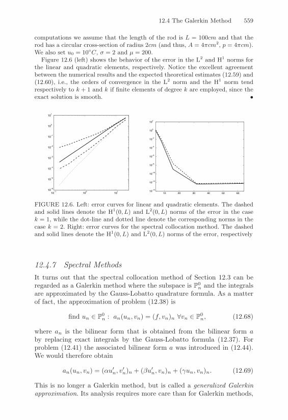
12.4 The Galerkin Method 559
computations we assume that the length of the rod is L = 100cm and that therod has a circular cross-section of radius 2cm (and thus, A = 4+cm2, p = 4+cm).We also set u0 = 10+C, ' = 2 and µ = 200.
Figure 12.6 (left) shows the behavior of the error in the L2 and H1 norms forthe linear and quadratic elements, respectively. Notice the excellent agreementbetween the numerical results and the expected theoretical estimates (12.59) and(12.60), i.e., the orders of convergence in the L2 norm and the H1 norm tendrespectively to k + 1 and k if finite elements of degree k are employed, since theexact solution is smooth. •
10!1
100
101
10!6
10!5
10!4
10!3
10!2
10!1
100
101
10 20 30 40 50 6010
!14
10!12
10!10
10!8
10!6
10!4
10!2
100
102
FIGURE 12.6. Left: error curves for linear and quadratic elements. The dashedand solid lines denote the H1(0, L) and L2(0, L) norms of the error in the casek = 1, while the dot-line and dotted line denote the corresponding norms in thecase k = 2. Right: error curves for the spectral collocation method. The dashedand solid lines denote the H1(0, L) and L2(0, L) norms of the error, respectively
12.4.7 Spectral MethodsIt turns out that the spectral collocation method of Section 12.3 can beregarded as a Galerkin method where the subspace is P0
n and the integralsare approximated by the Gauss-Lobatto quadrature formula. As a matterof fact, the approximation of problem (12.38) is
find un ! P0n : an(un, vn) = (f, vn)n #vn ! P0
n, (12.68)
where an is the bilinear form that is obtained from the bilinear form aby replacing exact integrals by the Gauss-Lobatto formula (12.37). Forproblem (12.41) the associated bilinear form a was introduced in (12.44).We would therefore obtain
an(un, vn) = ("u*n, v
*n)n + (#u*
n, vn)n + ('un, vn)n. (12.69)
This is no longer a Galerkin method, but is called a generalized Galerkinapproximation. Its analysis requires more care than for Galerkin methods,

560 12. Two-Point Boundary Value Problems
as already seen in Section 12.3 and depends on the Strang lemma (see[QV94]). However, the same kind of error estimate (12.39) can be provenin this case as well.
A further generalization combining the finite element approach withpiecewise polynomials of high degree and Gauss-Lobatto integration oneach element yields the so-called spectral element method and the h " pversion of the finite element method (here p stands for the polynomial de-gree that we have denoted with n). In these cases convergence is achievedletting simultaneously (or independently) h go to zero and p go to infinity.(See, e.g., [BM92], [SS98]).
Example 12.2 We consider again the two-point boundary value problem (12.67)and employ the spectral collocation method for its numerical approximation.We show in Figure 12.6 (right) the error curves in the L2(0, L) (solid line) andH1(0, L) (dashed line) norms as functions of the spectral degree n, with n = 4%k,k = 1, . . . , 5. Notice the high accuracy that is achieved, even when a small valueof n is used, due to the smoothness of the exact solution. Notice also that forn ! 32 the accuracy is actually bounded by the e"ect of rounding errors. •
12.5 Advection-Di"usion Equations
Boundary value problems of the form (12.41) are used to describe processesof di!usion, advection and absorption (or reaction) of a certain quantitywhich is identified with u(x). The term "("u*)* is responsible for the di!u-sion, #u* for the advection (or transport), 'u for the absorption (if ' > 0).In this section we focus on the case where " is small compared with # (or'). In these cases, the Galerkin method that we introduced earlier mightbe unsuitable for providing accurate numerical results. A heuristic explana-tion can be drawn from the inequality (12.56), noticing that in this case theconstant M/"0 can be very large, hence the error estimate can be mean-ingless unless h is much smaller than (M/"0)"1. For instance, if " = +,' = 0 and # = const 4 1, then "0 = + and M = + + CP#. Similarly, if" = +, # = 0 and ' = const4 1 then "0 = + and M = ++ C2
P '.
To keep our analysis at the simplest possible level, we will consider thefollowing elementary two-point boundary value problem
B "+u** + #u* = 0, 0 < x < 1,
u(0) = 0, u(1) = 1,(12.70)
where + and # are two positive constants such that +/# : 1. Despiteits simplicity, (12.70) provides an interesting paradigm of an advection-di!usion problem in which advection dominates di!usion.

12.5 Advection-Di"usion Equations 561
We define the global Peclet number as
Pegl =|#|L2+
(12.71)
where L is the size of the domain (equal to 1 in our case). The global Pecletnumber measures the dominance of the advective term over the di!usiveone.
Let us first compute the exact solution of problem (12.70). The charac-teristic equation associated to the di!erential equation is "+$2 + #$ = 0and admits the roots $1 = 0 and $2 = #/+. Then
u(x) = C1e#1x + C2e
#2x = C1 + C2e#$ x,
where C1 and C2 are arbitrary constants. Imposing the boundary conditionsyields C1 = "1/(e'/% " 1) = "C2, therefore
u(x) = (exp(#x/+)" 1) / (exp(#/+)" 1) .
If #/+: 1 we can expand the exponentials up to first order obtaining
u(x) = (1 +#
+x + · · ·" 1)/(1 +
#
++ · · ·" 1) 1 (# x/+)/(#/+) = x,
thus the solution is close to the solution of the limit problem "+u** = 0,which is a straight line interpolating the boundary data.However, if #/+4 1 the exponentials attain big values so that
u(x) 1 exp(#/+x)exp(#/+)
= exp-"#+(1" x)
..
Since the exponent is big and negative the solution is almost equal to zeroeverywhere unless a small neighborhood of the point x = 1 where theterm 1 " x becomes very small and the solution joins the value 1 with anexponential behaviour. The width of the neighbourhood is of the order of+/# and thus it is quite small: in such an event, we say that the solutionexhibits a boundary layer of width O (+/#) at x = 1.
12.5.1 Galerkin Finite Element ApproximationLet us discretize problem (12.70) using the Galerkin finite element methodintroduced in Section 12.4.5 with k = 1 (piecewise linear finite elements).The approximation to the problem is: find uh ! X1
h such that)+
,a(uh, vh) = 0 #vh ! X1,0
h ,
uh(0) = 0, uh(1) = 1,(12.72)

562 12. Two-Point Boundary Value Problems
where the finite element spaces X1h and X1,0
h have been introduced in (8.22)and (12.57) and the bilinear form a(·, ·) is
a(uh, vh) =^ 1
0(+u*
hv*h + #u*
hvh) dx. (12.73)
Remark 12.5 (Advection-di!usion problems in conservation form)Sometimes, the advection-di!usion problem (12.70) is written in the follow-ing conservation form
B "(J(u))* = 0, 0 < x < 1,
u(0) = 0, u(1) = 1,(12.74)
where J(u) = +u*"#u is the flux (already introduced in the finite di!erencecontext in Section 12.2.3), + and # are given functions with +(x) ) +0 > 0for all x ! [0, 1]. The Galerkin approximation of (12.74) using piecewiselinear finite elements reads: find uh ! X1
h such that
b(uh, vh) = 0, #vh ! X1,0h
where b(uh, vh) =1^
0
(+u*h " #uh)v*h dx. The bilinear form b(·, ·) coincides
with the corresponding one in (12.73) when + and # are constant. !
Taking vh as a test function the generic basis function 1i, (12.72) yields
1^
0
+u*h1
*i dx +
1^
0
#u*h1i dx = 0 i = 1, . . . , n" 1.
Setting uh(x) =!n
j=0 uj1j(x), and noting that supp(1i) = [xi"1, xi+1] theabove integral, for i = 1, . . . , n" 1, reduces to
+
"
$ui"1
xi^
xi"1
1*i"11
*i dx + ui
xi+1^
xi"1
(1*i)
2dx + ui+1
xi+1^
xi
1*i1
*i+1 dx
%
'
+#
"
$ui"1
xi^
xi"1
1*i"11i dx + ui
xi+1^
xi"1
1*i1i dx + ui+1
xi+1^
xi
1*i+11i dx
%
' = 0.
Assuming a uniform partition of [0, 1] with xi = xi"1 + h for i = 1, . . . , n,h = 1/n, and noting that 1*
j(x) = 1h if xj"1 & x & xj , 1*
j(x) = " 1h if
xj & x & xj+1, we deduce that
+
h("ui"1 + 2ui " ui+1) +
12# (ui+1 " ui"1) = 0, i = 1, . . . , n" 1.
(12.75)

12.5 Advection-Di"usion Equations 563
Multiplying by h/+ and defining the local Peclet number to be
Pe =|#|h2+
we finally obtain
(Pe" 1)ui+1 + 2ui " (Pe + 1)ui"1 = 0. i = 1, . . . , n" 1. (12.76)
This is a linear di!erence equation which admits a solution of the formui = A1)i1 + A2)i2 for suitable constants A1, A2 (see Section 11.4), where)1 and )2 are the two roots of the following characteristic equation
(Pe" 1) )2 + 2)" (Pe + 1) = 0.
Thus
)1,2 ="1 ±
/1 + Pe2 " 1
Pe" 1=
)+
,
1 + Pe1" Pe
,
1.
Imposing the boundary conditions at x = 0 and x = 1 gives
A1 = 1/(1"K
1+Pe1"Pe
Ln), A2 = "A1,
so that the solution of (12.76) is
ui =
6
1"4
1 + Pe1" Pe
5i7
/
41"
41 + Pe1" Pe
5n5i = 0, . . . , n.
We notice that if Pe > 1, a power with a negative base appears at thenumerator which gives rise to an oscillating solution. This is clearly visiblein Figure 12.7 where for several values of the local Peclet number, thesolution of (12.76) is compared with the exact solution (sampled at themesh nodes) corresponding to a value of the global Peclet equal to 50.
The simplest remedy for preventing the oscillations consists of choosinga su"ciently small mesh stepsize h in such a way that Pe < 1. However thisapproach is often impractical: for example, if # = 1 and + = 5 · 10"5 oneshould take h < 10"4 which amounts to dividing [0, 1] into 10000 subin-tervals, a strategy that becomes unfeasible when dealing with multidimen-sional problems. Other strategies can be pursued, as will be addressed inthe next sections.
12.5.2 The Relationship between Finite Elements and FiniteDi!erences; the Numerical Viscosity
To examine the behaviour of the finite di!erence method (FD) when appliedto the solution of advection-di!usion problems and its relationship with the

564 12. Two-Point Boundary Value Problems
0.75 0.8 0.85 0.9 0.95 1
!0.5
0
0.5
1
FIGURE 12.7. Finite di"erence solution of the advection-di"usion problem(12.70) (with Pegl = 50) for several values of the local Peclet number. Solidline: exact solution, dot-dashed line: Pe = 2.63, dotted line: Pe = 1.28, dashedline: Pe = 0.63
finite element method (FE), we again consider the one-dimensional problem(12.70) with a uniform meshsize h.
To ensure that the local discretization error is of second order we approx-imate u*(xi) and u**(xi), i = 1, . . . , n" 1, by the centred finite di!erences(10.61) and (10.65) respectively (see Section 10.10.1). We obtain the fol-lowing FD problem)+
,"+ui+1 " 2ui + ui"1
h2 + #ui+1 " ui"1
2h= 0, i = 1, . . . , n" 1
u0 = 0, un = 1.(12.77)
If we multiply by h for every i = 1, . . . , n" 1, we obtain exactly the sameequation (12.75) that was obtained using piecewise linear finite elements.
The equivalence between FD and FE can be profitably employed to de-vise a cure for the oscillations arising in the approximate solution of (12.75)when the local Peclet number is larger than 1. The important observationhere is that the instability in the FD solution is due to the fact that thediscretization scheme is a centred one. A possible remedy consists of ap-proximating the first derivative by a one-sided finite di!erence accordingto the direction of the transport field. Precisely, we use the backward dif-ference if the convective coe"cient # is positive and the forward di!erenceotherwise. The resulting scheme when # > 0 is
"+ui+1 " 2ui + ui"1
h2 + #ui " ui"1
h= 0 i = 1, . . . , n" 1 (12.78)
which, for + = 0 reduces to ui = ui"1 and therefore yields the desiredconstant solution of the limit problem #u* = 0. This one-side discretization
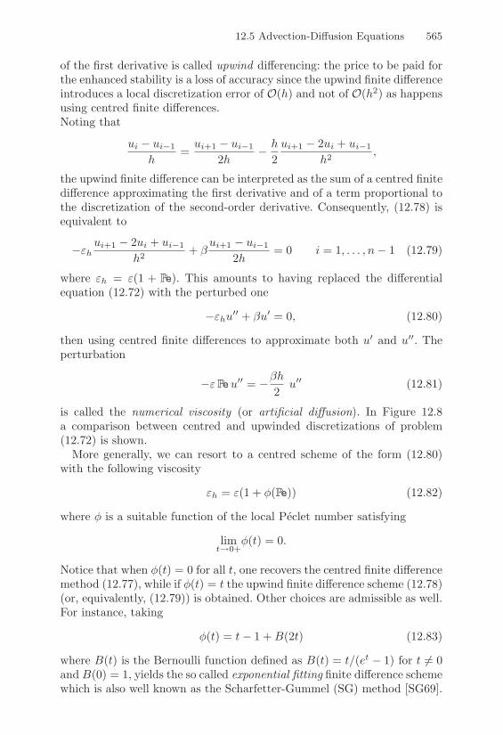
12.5 Advection-Di"usion Equations 565
of the first derivative is called upwind di!erencing: the price to be paid forthe enhanced stability is a loss of accuracy since the upwind finite di!erenceintroduces a local discretization error of O(h) and not of O(h2) as happensusing centred finite di!erences.Noting that
ui " ui"1
h=
ui+1 " ui"1
2h" h
2ui+1 " 2ui + ui"1
h2 ,
the upwind finite di!erence can be interpreted as the sum of a centred finitedi!erence approximating the first derivative and of a term proportional tothe discretization of the second-order derivative. Consequently, (12.78) isequivalent to
"+hui+1 " 2ui + ui"1
h2 + #ui+1 " ui"1
2h= 0 i = 1, . . . , n" 1 (12.79)
where +h = +(1 + Pe). This amounts to having replaced the di!erentialequation (12.72) with the perturbed one
"+hu** + #u* = 0, (12.80)
then using centred finite di!erences to approximate both u* and u**. Theperturbation
"+Peu** = "#h2
u** (12.81)
is called the numerical viscosity (or artificial di!usion). In Figure 12.8a comparison between centred and upwinded discretizations of problem(12.72) is shown.
More generally, we can resort to a centred scheme of the form (12.80)with the following viscosity
+h = +(1 + 4(Pe)) (12.82)
where 4 is a suitable function of the local Peclet number satisfying
limt&0+
4(t) = 0.
Notice that when 4(t) = 0 for all t, one recovers the centred finite di!erencemethod (12.77), while if 4(t) = t the upwind finite di!erence scheme (12.78)(or, equivalently, (12.79)) is obtained. Other choices are admissible as well.For instance, taking
4(t) = t" 1 + B(2t) (12.83)
where B(t) is the Bernoulli function defined as B(t) = t/(et " 1) for t '= 0and B(0) = 1, yields the so called exponential fitting finite di!erence schemewhich is also well known as the Scharfetter-Gummel (SG) method [SG69].
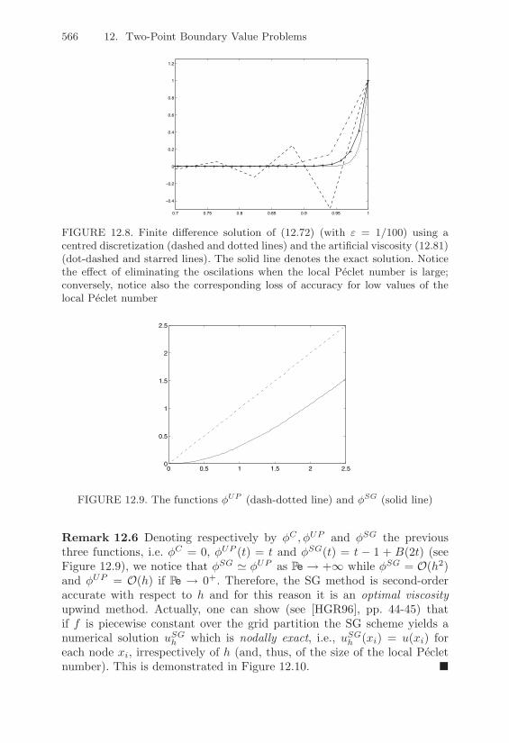
566 12. Two-Point Boundary Value Problems
0.7 0.75 0.8 0.85 0.9 0.95 1
!0.4
!0.2
0
0.2
0.4
0.6
0.8
1
1.2
FIGURE 12.8. Finite di"erence solution of (12.72) (with & = 1/100) using acentred discretization (dashed and dotted lines) and the artificial viscosity (12.81)(dot-dashed and starred lines). The solid line denotes the exact solution. Noticethe e"ect of eliminating the oscilations when the local Peclet number is large;conversely, notice also the corresponding loss of accuracy for low values of thelocal Peclet number
0 0.5 1 1.5 2 2.50
0.5
1
1.5
2
2.5
FIGURE 12.9. The functions 3UP (dash-dotted line) and 3SG (solid line)
Remark 12.6 Denoting respectively by 4C ,4UP and 4SG the previousthree functions, i.e. 4C = 0, 4UP (t) = t and 4SG(t) = t " 1 + B(2t) (seeFigure 12.9), we notice that 4SG 1 4UP as Pe ( +, while 4SG = O(h2)and 4UP = O(h) if Pe ( 0+. Therefore, the SG method is second-orderaccurate with respect to h and for this reason it is an optimal viscosityupwind method. Actually, one can show (see [HGR96], pp. 44-45) thatif f is piecewise constant over the grid partition the SG scheme yields anumerical solution uSG
h which is nodally exact, i.e., uSGh (xi) = u(xi) for
each node xi, irrespectively of h (and, thus, of the size of the local Pecletnumber). This is demonstrated in Figure 12.10. !

12.5 Advection-Di"usion Equations 567
0.9 0.95 1
0
0.5
1
FIGURE 12.10. Comparison between the numerical solutions of problem (12.72)(with & = 1/200) obtained using the artificial viscosity (12.81) (dashed line wherethe symbol ! denotes the nodal values) and with the optimal viscosity (12.83)(dotted line where the symbol 9 denotes the nodal values) in the case wherePe = 1.25. The solid line denotes the exact solution
The new local Peclet number associated with the scheme (12.79)-(12.82) isdefined as
Pe, =|#|h2+h
=Pe
(1 + 4(Pe)).
For both the upwind and the SG schemes we have Pe, < 1 for any valueof h. This implies that the matrix associated with these methods is a M-matrix for any h (see Definition 1.25 and Exercise 13), and, in turn, that thenumerical solution uh satisfies a discrete maximum principle (see Section12.2.2).
12.5.3 Stabilized Finite Element MethodsIn this section we extend the use of numerical viscosity introduced inthe previous section for finite di!erences to the Galerkin method usingfinite elements of arbitrary degree k ) 1. For this purpose we considerthe advection-di!usion problem (12.70) where the viscosity coe"cient + isreplaced by (12.82). This yields the following modification of the originalGalerkin problem (12.72):
find 0uh! Xk,0
h =/vh ! Xk
h : vh(0) = vh(1) = 00
such that
ah( 0uh, vh) = "
1^
0
#vh dx #vh ! Xk,0h , (12.84)
whereah(u, v) = a(u, v) + b(u, v),
568 12. Two-Point Boundary Value Problems
and
b(u, v) = + 4(Pe)1^
0
u*v* dx
is called the stabilization term. Since ah(v, v) = +h|v|21 for all v ! H10(0, 1)
and +h/+ = (1 + 4(Pe)) ) 1, the modified problem (12.84) enjoys morefavorable monotonicity properties than the corresponding non stabilizedGalerkin formulation (12.75).
To prove convergence, it is su"cient to show that 0uh tends to
0u as h( 0,
where0u (x) = u(x) " x. This is done in the following theorem, where we
assume that0u (and henceforth u) has the required regularity.
Theorem 12.4 If k = 1 then
| 0u " 0
uh |H1(0,1) & Ch G(0u) (12.85)
where C > 0 is a suitable constant independent of h and0u, and
G(0u) =
)*+
*,
| 0u |H1(0,1) + | 0
u |H2(0,1) for the upwind method
| 0u |H2(0,1) for the SG method.
Further, if k = 2 the SG method yields the improved error estimate
| 0u " 0
uh |H1(0,1) & Ch2(| 0u |H1(0,1) + | 0
u |H3(0,1)). (12.86)
Proof. From (12.70) we obtain
a(0u, vh) = %
1^
0
)vhdx, )vh / Xk,0h .
By comparison with (12.84) we get
ah(0u % 0
uh, vh) = b(0u, vh), )vh / Xk,0
h . (12.87)
Denote by Eh =0u % 0
uh the discretization error and recall that the space H10(0, 1)
is endowed with the norm (12.49). Then,
&h|Eh|2H1(0,1) = ah(Eh, Eh) = ah(Eh,0u %(k
h0u) + ah(Eh,(k
h0u % 0
uh)
= ah(Eh,0u %(k
h0u) + b(
0u,(k
h0u % 0
uh)
where we have applied (12.87) with vh = (kh
0u % 0
uh. Using the Cauchy-Schwarzinequality we get
&h|Eh|2H1(0,1) "Mh|Eh|H1(0,1)|0u %(k
h0u |H1(0,1)
+&3(Pe)1^
0
0u(((k
h0u % 0
uh)(dx(12.88)
12.5 Advection-Di"usion Equations 569
where Mh = &h + |)|CP is the continuity constant of the bilinear form ah(·, ·)and CP is the Poincare constant introduced in (12.16).
Notice that if k = 1 (corresponding to piecewise linear finite elements) and3 = 3SG (SG optimal viscosity) the quantity in the second integral is identicallyzero since 0
uh= (1h
0u, as pointed out in Remark 12.6. Then, from (12.88) we get
|Eh|H1(0,1) "4
1 +|)|CP
&h
5| 0u %(1
h0u |H1(0,1).
Noting that &h > &, using (12.71) and the interpolation estimate (8.27), we finallyobtain the error bound
|Eh|H1(0,1) " C(1 + 2PeglCP )h| 0u |H2(0,1).
In the general case the error inequality (12.88) can be further manipulated. Usingthe Cauchy-Schwarz and triangular inequalities we obtain
1^
0
0u(((k
h0u % 0
uh)(dx " | 0u |H1(0,1)(|(k
h0u % 0
u |H1(0,1) + |Eh|H1(0,1))
from which
&h|Eh|2H1(0,1) " |Eh|H1(0,1)
KMh|
0u %(k
h0u |H1(0,1)
+&3(Pe)| 0u |H1(0,1)
L+ &3(Pe)| 0
u |H1(0,1)|0u %(k
h0u |H1(0,1).
Using again the interpolation estimate (8.27) yields
&h|Eh|2H1(0,1) " |Eh|H1(0,1)
KMhChk| 0
u |Hk+1(0,1) + &3(Pe)| 0u |H1(0,1)
L
+C&3(Pe)| 0u |H1(0,1)h
k| 0u |Hk+1(0,1).
Using Young’s inequality (12.40) gives
&h|Eh|2H1(0,1) "&h|Eh|2H1(0,1)
2
+3
4&h
V(MhChk| 0
u |Hk+1(0,1))2 + (&3(Pe)| 0
u |H1(0,1))2W
from which it follows that
|Eh|2H1(0,1) " 32
4Mh
&h
52
C2h2k| 0u |2Hk+1(0,1) +
32
4&&h
52
3(Pe)2| 0u |2H1(0,1)
+2&&h
3(Pe)| 0u |H1(0,1)Chk| 0
u |Hk+1(0,1).
Again using the fact that &h > & and the definition (12.71) we get (Mh/&h) "(1 + 2CP Pegl) and then
|Eh|2H1(0,1) " 32C2(1 + 2CP Pegl)2h2k| 0
u |2Hk+1(0,1)
+23(Pe)Chk| 0u |H1(0,1)|
0u |Hk+1(0,1) +
323(Pe)2| 0
u |2H1(0,1),

570 12. Two-Point Boundary Value Problems
which can be bounded further as
|Eh|2H1(0,1) " MVh2k| 0
u |2Hk+1(0,1)
+ 3(Pe)hk| 0u |H1(0,1)|
0u |Hk+1(0,1) + 3(Pe)2| 0
u |2H1(0,1)
W (12.89)
for a suitable positive constant M.If 3UP = C'h, where C' = )/&, we obtain
|Eh|2H1(0,1) " Ch2Vh2k%2| 0
u |2Hk+1(0,1)
+hk%1| 0u |H1(0,1)|
0u |Hk+1(0,1) + | 0
u |2H1(0,1)
W
which shows that using piecewise linear finite elements (i.e., k = 1) plus theupwind artificial viscosity gives the linear convergence estimate (12.85).In the case 3 = 3SG, assuming that for h su!ciently small 3SG " Kh2, for asuitable positive constant K, we get
|Eh|2H1(0,1) " Ch4Vh2(k%2)| 0
u |2Hk+1(0,1)
+hk%2| 0u |H1(0,1)|
0u |Hk+1(0,1) + | 0
u |2H1(0,1)
W
which shows that using quadratic finite elements (i.e., k = 2) plus the optimalartificial viscosity gives the second-order convergence estimate (12.86). !
Programs 97 and 98 implement the computation of the artificial and opti-mal artificial viscosities (12.81) and (12.83), respectively. These viscositiescan be selected by the user setting the input parameter stabfun in Pro-gram 94 equal to artvisc or sgvisc. The function sgvisc employs thefunction bern to evaluate the Bernoulli function in (12.83).
Program 97 - artvisc : Artificial viscosity
function [Kupw,rhsbc] = artvisc(Nx, h, nu, beta)Peclet=0.5*h*abs(beta);for i=2:Nx,
dd(i-1)=(Peclet(i-1)+Peclet(i))/h;if i > 2, ld(i-2)=-Peclet(i-1)/h; endif i < Nx, ud(i-1)=-Peclet(i)/h; end
endKupw=spdiags([[ld 0]’,dd’,[0 ud]’],-1:1,Nx-1,Nx-1);rhsbc = - [Peclet(1)/h, Peclet(Nx)/h];
Program 98 - sgvisc : Optimal artificial viscosity
function [Ksg,rhsbc] = sgvisc(Nx, h, nu, beta)Peclet=0.5*h*abs(beta)./nu;[bp, bn]=bern(2*Peclet);Peclet=Peclet-1+bp;

12.5 Advection-Di"usion Equations 571
for i=2:Nx,dd(i-1)=(nu(i-1)*Peclet(i-1)+nu(i)*Peclet(i))/h;if i > 2, ld(i-2)=-nu(i-1)*Peclet(i-1)/h; endif i < Nx, ud(i-1)=-nu(i)*Peclet(i)/h; end
endKsg=spdiags([[ld 0]’,dd’,[0 ud]’],-1:1,Nx-1,Nx-1);rhsbc = - [nu(1)*Peclet(1)/h, nu(Nx)*Peclet(Nx)/h];
Program 99 - bern : Evaluation of the Bernoulli function
function [bp,bn]=bern(x)xlim=1e-2; ax=abs(x);if (ax == 0), bp=1.; bn=1.; return; end;if (ax > 80),
if (x > 0), bp=0.; bn=x; return;else, bp=-x; bn=0.; return; end;
end;if (ax > xlim),
bp=x/(exp(x)-1); bn=x+bp; return;else
ii=1; fp=1.;fn=1.; df=1.; s=1.;while (abs(df) > eps),ii=ii+1; s=-s; df=df*x/ii;fp=fp+df; fn=fn+s*df;bp=1./fp; bn=1./fn;
end;return;
end
Example 12.3 We use Program 94 supplied with Programs 97 and 98 for thenumerical approximation of problem (12.70) in the case & = 10%2. Figure 12.11shows the convergence behavior as a function of log(h) of the Galerkin methodwithout (G) and with numerical viscosity (upwind (UP) and SG methods areemployed). The figure shows the logarithmic plots of the L2(0, 1) and H1(0, 1)-norms, where the solid line denotes the UP method and the dashed and dottedlines denote the G and SG methods, respectively. It is interesting to notice thatthe UP and SG schemes exhibit the same (linear) convergence rate as the pureGalerkin method in the H1-norm, while the accuracy of the UP scheme in theL2-norm deteriorates dramatically because of the e"ect of the artificial viscositywhich is O(h). Conversely, the SG converges quadratically since the introducednumerical viscosity is in this case O(h2) as h tends to zero. •

572 12. Two-Point Boundary Value Problems
10!3 10!2 10!110!4
10!3
10!2
10!1
100
101
102
||u ! u h ||L2(0,1)
||u ! uh ||H1(0,1)
FIGURE 12.11. Convergence analysis for an advection-di"usion problem
12.6 A Quick Glance to the Two-Dimensional Case
The game that we want to play is to extend (in a few pages) the basic ideasillustrated so far to the two-dimensional case. The obvious generalization ofproblem (12.1)-(12.2) is the celebrated Poisson problem with homogeneousDirichlet boundary condition
B "=u = f in (,
u = 0 on .(,(12.90)
where =u = .2u/.x2 + .2u/.y2 is the Laplace operator and ( is a two-dimensional bounded domain whose boundary is .(. If we allow ( to bethe unit square ( = (0, 1)2, the finite di!erence approximation of (12.90)that mimics (12.10) is
BLhuh(xi,j) = f(xi,j) for i, j = 1, . . . , N " 1,
uh(xi,j) = 0 if i = 0 or N, j = 0 or N,(12.91)
where xi,j = (ih, jh) (h = 1/N > 0) are the grid points and uh is a gridfunction. Finally, Lh denotes any consistent approximation of the operatorL = "=. The classical choice is
Lhuh(xi,j) =1h2 (4ui,j " ui+1,j " ui"1,j " ui,j+1 " ui,j"1) , (12.92)
where ui,j = uh(xi,j), which amounts to adopting the second-order centreddiscretization of the second derivative (10.65) in both x and y directions(see Figure 12.12, left).
The resulting scheme is known as the five-point discretization of theLaplacian. It is an easy (and useful) exercise for the reader to check thatthe associated matrix Afd has (N"1)2 rows and is pentadiagonal, with the

12.6 A Quick Glance to the Two-Dimensional Case 573
xij xi,j+1
xi+1,j
xi,j!1
xi!1,j
FIGURE 12.12. Left: finite di"erence grid and stencil for a squared domain.Right: finite element triangulation of a region around a hole
i-th row given by
(afd)ij =1h2
)**+
**,
4 if j = i,
"1 if j = i"N " 1, i" 1, i + 1, i + N + 1,
0 otherwise.
(12.93)
Moreover, Afd is symmetric positive definite and it is also an M-matrix (seeExercise 14). As expected, the consistency error associated with (12.92) issecond-order with respect to h, and the same holds for the discretizationerror +u" uh+h,$ of the method. More general boundary conditions thanthe one considered in (12.90) can be dealt with by properly extending tothe two-dimensional case the mirror imaging technique described in Section12.2.3 and in Exercise 10 (for a thorough discussion of this subject, see, e.g.,[Smi85]).
The extension of the Galerkin method is (formally speaking) even morestraightforward and actually is still readable as (12.43) with, however, theimplicit understanding that both the function space Vh and the bilinearform a(·, ·) be adapted to the problem at hand. The finite element methodcorresponds to taking
Vh =/vh ! C0(() : vh|T ! Pk(T )#T ! Th, vh|%! = 0
0, (12.94)
where Th denotes here a triangulation of the domain ( as previously intro-duced in Section 8.5.2, while Pk (k ) 1) is the space of piecewise polyno-mials defined in (8.35). Note that ( needs not to be a rectangular domain(see Figure 12.12, right).

574 12. Two-Point Boundary Value Problems
As of the bilinear form a(·, ·), the same kind of mathematical manipula-tions performed in Section 12.4.1 lead to
a(uh, vh) =^
"
5uh ·5vh dxdy,
where we have used the following Green’s formula that generalizes theformula of integration by parts
^
"
"=u v dxdy =^
"
5u ·5v dxdy "^
)"
5u · n v d', (12.95)
for any u, v smooth enough and where n is the outward normal unit vectoron .( (see Exercise 15).
The error analysis for the two-dimensional finite element approximationof (12.90) can still be performed through the combined use of Cea’s lemmaand interpolation error estimates as in Section 12.4.5 and is summarized inthe following result, which is the two-dimensional counterpart of Property12.1 (for its proof we refer, e.g., to [QV94], Theorem 6.2.1).
Property 12.2 Let u ! H10(() be the exact solution of (12.90) and uh ! Vh
be its finite element approximation using continuous piecewise polynomialsof degree k ) 1. Assume also that u ! Hs(() for some s ) 2. Then thefollowing error estimate holds
+u" uh+H10(") &
M
"0Chl+u+Hl+1(") (12.96)
where l = min(k, s " 1). Under the same assumptions, one can also provethat
+u" uh+L2(") & Chl+1+u+Hl+1("). (12.97)
We notice that, for any integer s ) 0, the Sobolev space Hs(() introducedabove is defined as the space of functions with the first s partial derivatives(in the distributional sense) belonging to L2((). Moreover, H1
0(() is thespace of functions of H1(() such that u = 0 on .(. The precise mathemat-ical meaning of this latter statement has to be carefully addressed since,for instance, a function belonging to H1
0(() does not necessarily mean tobe continuous everywhere. For a comprehensive presentation and analysisof Sobolev spaces we refer to [Ada75] and [LM68].
Following the same procedure as in Section 12.4.3, we can write the finiteelement solution uh as
uh(x, y) =N(
j=1
uj1j(x, y)
12.7 Applications 575
where {1j}Nj=1 is a basis for Vh. An example of such a basis in the casek = 1 is provided by the so-called hat functions introduced in Section 8.5.2(see Figure 8.7, right). The Galerkin finite element method leads to thesolution of the linear system Afeu = f , where (afe)ij = a(1j ,1i).
Exactly as happens in the one-dimensional case, the matrix Afe is sym-metric positive definite and, in general, sparse, the sparsity pattern beingstrongly dependent on the topology of Th and the numbering of its nodes.Moreover, the spectral condition number of Afe is still O(h"2), which im-plies that solving iteratively the linear system demands for the use of asuitable preconditioner (see Section 4.3.2). If, instead, a direct solver isused, one should resort to a suitable renumbering procedure, as explainedin Section 3.9.
12.7 Applications
In this section we employ the finite element method for the numericalapproximation of two problems arising in fluid mechanics and in the sim-ulation of biological systems.
12.7.1 Lubrication of a SliderLet us consider a rigid slider moving in the direction x along a physicalsupport from which it is separated by a thin layer of a viscous fluid (whichis the lubricant). Suppose that the slider, of length L, moves with a ve-locity U with respect to the plane support which is supposed to have aninfinite length. The surface of the slider that is faced towards the supportis described by the function s (see Figure 12.13, left).Denoting by µ the viscosity of the lubricant, the pressure p acting on theslider can be modeled by the following Dirichlet problem
)*+
*,"
4s3
6µp*
5*
= "(Us)* x ! (0, L),
p(0) = 0, p(L) = 0.
Assume in the numerical computations that we are working with a conver-gent-divergent slider of unit length, whose surface is s(x) = 1"3/2x+9/8x2
with µ = 1.Figure 12.13 (right) shows the solution obtained using linear and quadratic
finite elements with an uniform grid size h = 0.2. The linear system hasbeen solved by the nonpreconditioned conjugate gradient method. To re-duce the Euclidean norm of the residual below 10"10, 4 iterations areneeded in the case of linear finite elements while 9 are required for quadraticfinite elements.

576 12. Two-Point Boundary Value Problems
L
s(x)
U
x
0 0.1 0.2 0.3 0.4 0.5 0.6 0.7 0.8 0.9 1!0.01
0
0.01
0.02
0.03
0.04
0.05
0.06
0.07
0.08
0.09
FIGURE 12.13. Left: geometrical parameters of the slider considered in Section12.7.1; right: pressure on a converging-diverging slider. The solid line denotesthe solution obtained used linear finite elements (the symbol 9 denotes the nodalvalues), while the dashed line denotes the solution obtained using quadratic finiteelements
Table 12.2 reports a numerical study of the condition number K2(Afe) asa function of h. In the case of linear finite elements we have denoted thematrix by A1, while A2 is the corresponding matrix for quadratic elements.Here we assume that the condition number approaches h"p as h tends tozero; the numbers pi are the estimated values of p. As can be seen, inboth cases the condition number grows like h"2, however, for every fixedh, K2(A2) is much bigger than K2(A1).
h K2(A1) p1 K2(A2) p20.10000 63.951 – 455.240.05000 348.21 2.444 2225.7 2.280.02500 1703.7 2.290 10173.3 2.190.01250 7744.6 2.184 44329.6 2.120.00625 33579 2.116 187195.2 2.07
TABLE 12.2. Condition number of the sti"ness matrix for linear and quadraticfinite elements
12.7.2 Vertical Distribution of Spore Concentration overWide Regions
In this section we are concerned with di!usion and transport processes ofspores in the air, such as the endspores of bacteria and the pollen of flow-ering plants. In particular, we study the vertical concentration distributionof spores and pollen grains over a wide area. These spores, in addition tosettling under the influence of gravity, di!use passively in the atmosphere.

12.7 Applications 577
The basic model assumes the di!usivity 3 and the settling velocity # tobe given constants, the averaging procedure incorporating various physicalprocesses such as small-scale convection and horizontal advection-di!usionwhich can be neglected over a wide horizontal area. Denoting by x ) 0 thevertical direction, the steady-state distribution u(x) of the spore concen-tration is the solution of
B"3u** + #u* = 0 0 < x < H,
u(0) = u0, "3u*(H) + #u(H) = 0,(12.98)
where H is a fixed height at which we assume a vanishing Neumann condi-tion for the advective-di!usive flux "3u*+#u (see Section 12.4.1). Realisticvalues of the coe"cients are 3 = 10 m2s"1 and # = "0.03 ms"1; as foru0, a reference concentration of 1 pollen grain per m3 has been used in thenumerical experiments, while the height H has been set equal to 10 km.The global Peclet number is therefore Pegl = 15.
The Galerkin finite element method with piecewise linear finite elementshas been used for the approximation of (12.98). Figure 12.14 (left) showsthe solution computed by running Program 94 on a uniform grid with step-size h = H/10. The solution obtained using the (non stabilized) Galerkinformulation (G) is denoted by the solid line, while the dash-dotted anddashed lines refer to the Scharfetter-Gummel (SG) and upwind (UP) sta-bilized methods. Spurious oscillations can be noticed in the G solution whilethe one obtained using UP is clearly overdi!used with respect to the SGsolution that is nodally exact. The local Peclet number is equal to 1.5 inthis case. Taking h = H/100 yields for the pure Galerkin scheme a stableresult as shown in Figure 12.14 (right) where the solutions furnished by G(solid line) and UP (dashed line) are compared.
0 2000 4000 6000 8000 10000!0.2
0
0.2
0.4
0.6
0.8
1
1.2
0 200 400 600 800 1000 1200 1400 1600 18000
0.1
0.2
0.3
0.4
0.5
0.6
0.7
0.8
0.9
1
FIGURE 12.14. Vertical concentration of spores: G, SG and UP solutions withh = H/10 (left) and h = H/100 (right, where only the portion [0, 2000] is shown).The x-axis represents the vertical coordinate
578 12. Two-Point Boundary Value Problems
12.8 Exercises1. Consider the boundary value problem (12.1)-(12.2) with f(x) = 1/x. Using
(12.3) prove that u(x) = %x log(x). This shows that u / C2(0, 1) but u(0)is not defined and u(, u(( do not exist at x = 0 (*: if f / C0(0, 1), but notf / C0([0, 1]), then u does not belong to C0([0, 1])).
2. Prove that the matrix Afd introduced in (12.8) is an M-matrix.[Hint: check that Afdx ! 0* x ! 0. To do this, for any $ > 0 set Afd,! =Afd+$In%1. Then, compute w = Afd,!x and prove that min1*i*(n%1) wi !0. Finally, since the matrix Afd,! is invertible, being symmetric and positivedefinite, and since the entries of A%1
fd,! are continuous functions of $ ! 0,one concludes that A%1
fd,! is a nonnegative matrix as $, 0.]
3. Prove that (12.13) defines a norm for V 0h .
4. Prove (12.15) by induction on m.
5. Prove the estimate (12.23).[Hint: for each internal node xj , j = 1, . . . , n%1, integrate by parts (12.21)to get
4h(xj)
= %u(((xj)%1h2
"
#$
xj^
xj%h
u(((t)(xj % h% t)2 dt%xj+h^
xj
u(((t)(xj + h% t)2 dt
%
&' .
Then, pass to the squares and sum 4h(xj)2 for j = 1, . . . , n% 1. On notingthat (a+b+c)2 " 3(a2 +b2 +c2), for any real numbers a, b, c, and applyingthe Cauchy-Schwarz inequality yields the desired result.]
6. Prove that Gk(xj) = hG(xj , xk), where G is Green’s function introduced in(12.4) and Gk is its corresponding discrete counterpart solution of (12.4).[Solution: we prove the result by verifying that LhG = hek. Indeed, for afixed xk the function G(xk, s) is a straight line on the intervals [0, xk] and[xk, 1] so that LhG = 0 at every node xl with l = 0, . . . , k % 1 and l =k+1, . . . , n+1. Finally, a direct computation shows that (LhG)(xk) = 1/hwhich concludes the proof.]
7. Let g = 1 and prove that Thg(xj) = 12xj(1% xj).
[Solution: use the definition (12.25) with g(xk) = 1, k = 1, . . . , n % 1 andrecall that Gk(xj) = hG(xj , xk) from the exercise above. Then
Thg(xj) = h
"
$j(
k=1
xk(1% xj) +n%1(
k=j+1
xj(1% xk)
%
'
from which, after straightforward computations, one gets the desired re-sult.]
8. Prove Young’s inequality (12.40).
9. Show that &vh&h " &vh&h,! )vh / Vh.

12.8 Exercises 579
10. Consider the two-point boundary value problem (12.29) with the followingboundary conditions
#0u(0) + µ0u(0) = g0, #1u(1) + µ1u(1) = g1,
where #j , µj and gj are given data (j = 0, 1). Using the mirror imagingtechnique described in Section 12.2.3 write the finite di"erence discretiza-tion of the equations corresponding to the nodes x0 and xn.[Solution:
node x0 :4$1/2
h2 +,0
2+
$0#0
µ0h
5u0 % $1/2
u1
h2 =$0g0
µ0h+
f0
2,
node xn :4$n%1/2
h2 +,n
2+
$n#1
µ1h
5un % $n%1/2
un%1
h2 =$ng1
µ1h+
fn2.]
11. Discretize the fourth-order di"erential operator Lu(x) = %u(iv)(x) usingcentred finite di"erences.[Solution : apply twice the second order centred finite di"erence operatorLh defined in (12.9).]
12. Consider problem (12.41) with non homogeneous Neumann boundary con-ditions $u((0) = w0, $u((1) = w1. Show that the solution satisfies prob-lem (12.43) where V = H1(0, 1) and the right-hand side is replaced by(f, v)+w1v(1)%w0v(0). Derive the formulation in the case of mixed bound-ary conditions $u((0) = w0, u(1) = u1.
13. Using Property 1.19 prove that the matrices corresponding to the stabilizedfinite element method (12.79) using the upwind and SG artificial viscosities3UP and 3SG (see Section 12.5.2) are M-matrices irrespective of h.[Hint: let us denote respectively by AUP and ASG the two sti"ness matricescorrsponding to 3UP and 3SG. Take v(x) = 1 + x and set vi = 1 + xi,i = 0, . . . , n, being xi = ih, h = 1/n. Then, by a direct computation checkthat (AUPv)i ! ) > 0. As for the matrix ASG the same result can beproved by noting that B(%t) = t + B(t) for any t / R.]
14. Prove that the matrix Afd with entries given by (12.93) is symmetric pos-itive definite and it is also an M-matrix.[Solution: to show that Afd is positive definite, proceed as in the corre-sponding proof in Section 12.2, then proceed as in Exercise 2.]
15. Prove the Green’s formula (12.95).[Solution: first, notice that for any u, v su!ciently smooth, div(v8u) =v:u+8u ·8v. Then, integrate this relation over ) and use the divergence
theorem^
!
div(v8u) dxdy =^
$!
1u1n
v d,.]

13Parabolic and Hyperbolic InitialBoundary Value Problems
The final chapter of this book is devoted to the approximation of time-dependent partial di!erential equations. Parabolic and hyperbolic initial-boundary value problems will be addressed and either finite di!erences andfinite elements will be considered for their discretization.
13.1 The Heat Equation
The problem we are considering is how to find a function u = u(x, t) forx ! [0, 1] and t > 0 that satisfies the partial di!erential equation
.u
.t+ Lu = f 0 < x < 1, t > 0, (13.1)
subject to the boundary conditions
u(0, t) = u(1, t) = 0, t > 0 (13.2)
and the initial condition
u(x, 0) = u0(x) 0 & x & 1. (13.3)
The di!erential operator L is defined as
Lu = "3 .2u
.x2 . (13.4)
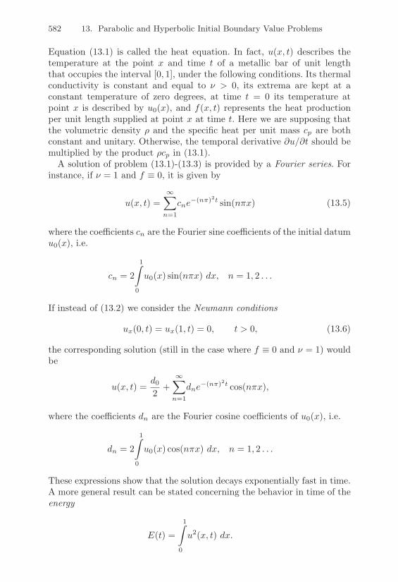
582 13. Parabolic and Hyperbolic Initial Boundary Value Problems
Equation (13.1) is called the heat equation. In fact, u(x, t) describes thetemperature at the point x and time t of a metallic bar of unit lengththat occupies the interval [0, 1], under the following conditions. Its thermalconductivity is constant and equal to 3 > 0, its extrema are kept at aconstant temperature of zero degrees, at time t = 0 its temperature atpoint x is described by u0(x), and f(x, t) represents the heat productionper unit length supplied at point x at time t. Here we are supposing thatthe volumetric density ) and the specific heat per unit mass cp are bothconstant and unitary. Otherwise, the temporal derivative .u/.t should bemultiplied by the product )cp in (13.1).
A solution of problem (13.1)-(13.3) is provided by a Fourier series. Forinstance, if 3 = 1 and f ? 0, it is given by
u(x, t) =$(
n=1
cne"(n")2t sin(n&x) (13.5)
where the coe"cients cn are the Fourier sine coe"cients of the initial datumu0(x), i.e.
cn = 21^
0
u0(x) sin(n&x) dx, n = 1, 2 . . .
If instead of (13.2) we consider the Neumann conditions
ux(0, t) = ux(1, t) = 0, t > 0, (13.6)
the corresponding solution (still in the case where f ? 0 and 3 = 1) wouldbe
u(x, t) =d0
2+
$(
n=1
dne"(n")2t cos(n&x),
where the coe"cients dn are the Fourier cosine coe"cients of u0(x), i.e.
dn = 21^
0
u0(x) cos(n&x) dx, n = 1, 2 . . .
These expressions show that the solution decays exponentially fast in time.A more general result can be stated concerning the behavior in time of theenergy
E(t) =1^
0
u2(x, t) dx.
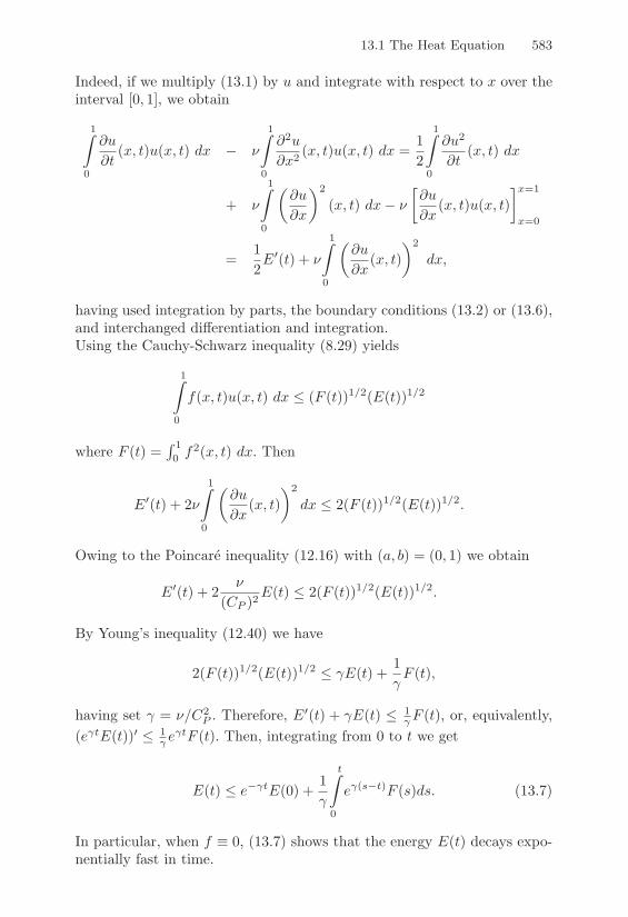
13.1 The Heat Equation 583
Indeed, if we multiply (13.1) by u and integrate with respect to x over theinterval [0, 1], we obtain
1^
0
.u
.t(x, t)u(x, t) dx " 3
1^
0
.2u
.x2 (x, t)u(x, t) dx =12
1^
0
.u2
.t(x, t) dx
+ 3
1^
0
4.u
.x
52
(x, t) dx" 3-.u
.x(x, t)u(x, t)
.x=1
x=0
=12E*(t) + 3
1^
0
4.u
.x(x, t)
52
dx,
having used integration by parts, the boundary conditions (13.2) or (13.6),and interchanged di!erentiation and integration.Using the Cauchy-Schwarz inequality (8.29) yields
1^
0
f(x, t)u(x, t) dx & (F (t))1/2(E(t))1/2
where F (t) =@ 10 f2(x, t) dx. Then
E*(t) + 231^
0
4.u
.x(x, t)
52
dx & 2(F (t))1/2(E(t))1/2.
Owing to the Poincare inequality (12.16) with (a, b) = (0, 1) we obtain
E*(t) + 23
(CP )2E(t) & 2(F (t))1/2(E(t))1/2.
By Young’s inequality (12.40) we have
2(F (t))1/2(E(t))1/2 & 'E(t) +1'F (t),
having set ' = 3/C2P . Therefore, E*(t) + 'E(t) & 1
-F (t), or, equivalently,(e-tE(t))* & 1
- e-tF (t). Then, integrating from 0 to t we get
E(t) & e"-tE(0) +1'
t^
0
e-(s"t)F (s)ds. (13.7)
In particular, when f ? 0, (13.7) shows that the energy E(t) decays expo-nentially fast in time.

584 13. Parabolic and Hyperbolic Initial Boundary Value Problems
13.2 Finite Di"erence Approximation of the HeatEquation
To solve the heat equation numerically we have to discretize both the xand t variables. We can start by dealing with the x-variable, following thesame approach as in Section 12.2. We denote by ui(t) an approximation ofu(xi, t), i = 0, . . . , n and approximate the Dirichlet problem (13.1)-(13.3)by the scheme
.ui (t)" 3
h2 (ui"1(t)" 2ui(t) + ui+1(t)) = fi(t), i = 1, . . . , n" 1,#t > 0,
u0(t) = un(t) = 0, #t > 0,
ui(0) = u0(xi), i = 0, . . . , n,
where the upper dot indicates derivation with respect to time, and fi(t) =f(xi, t). This is actually a semi-discretization of problem (13.1)-(13.3), andis a system of ordinary di!erential equations of the following form
Bu(t) = "3Afdu(t) + f(t), #t > 0,
u(0) = u0
(13.8)
where u(t) = (u1(t), . . . , un"1(t))T is the vector of unknowns, f(t) =(f1(t), . . . , fn"1(t))T , u0 = (u0(x1), . . . , u0(xn"1))T and Afd is the tridi-agonal matrix introduced in (12.8). Note that for the derivation of (13.8)we have assumed that u0(x0) = u0(xn) = 0, which is coherent with theboundary condition (13.2).
A popular scheme for the integration of (13.8) with respect to time is theso-called !"method. To construct the scheme, we denote by vk the valueof the variable v at time tk = k#t, for #t > 0; then, the !-method for thetime-integration of (13.8) is
)**+
**,
uk+1 " uk
#t= "3Afd(!uk+1 + (1" !)uk) + !fk+1 + (1" !)fk,
k = 0, 1, . . .u0 = u0
(13.9)
or, equivalently,
(I + 3!#tAfd)uk+1 = (I" 3#t(1" !)Afd)uk + gk+1, (13.10)
where gk+1 = #t(!fk+1 + (1 " !)fk) and I is the identity matrix of ordern" 1.
For suitable values of the parameter !, from (13.10) we can recover somefamiliar methods that have been introduced in Chapter 11. For example, if! = 0 the method (13.10) coincides with the forward Euler scheme and we

13.2 Finite Di"erence Approximation of the Heat Equation 585
can get uk+1 explicitly; otherwise, a linear system (with constant matrixI + 3!#tAfd) needs be solved at each time-step.
Regarding stability, assume that f ? 0 (henceforth gk = 0 #k > 0),so that from (13.5) the exact solution u(x, t) tends to zero for every xas t ( ,. Then we would expect the discrete solution to have the samebehaviour, in which case we would call our scheme (13.10) asymptoticallystable, this being coherent with what we did in Chapter 11, Section 11.1for ordinary di!erential equations.
If ! = 0, from (13.10) it follows that
uk = (I" 3#tAfd)ku0, k = 1, 2, . . .
From the analysis of convergent matrices (see Section 1.11.2) we deducethat uk ( 0 as k (, i!
)(I" 3#tAfd) < 1. (13.11)
On the other hand, the eigenvalues of Afd are given by (see Exercise 3)
µi =4h2 sin2(i&h/2), i = 1, . . . , n" 1.
Then (13.11) is satisfied i!
#t <123
h2.
As expected, the forward Euler method is conditionally stable, and thetime-step #t should decay as the square of the grid spacing h.
In the case of the backward Euler method (! = 1), we would have from(13.10)
uk =P(I + 3#tAfd)"1Qk u0, k = 1, 2, . . .
Since all the eigenvalues of the matrix (I+3#tAfd)"1 are real, positive andstrictly less than 1 for every value of #t, this scheme is unconditionallystable. More generally, the !-scheme is unconditionally stable for all thevalues 1/2 & ! & 1, and conditionally stable if 0 & ! < 1/2 (see Section13.3.1).
As far as the accuracy of the !-method is concerned, its local truncationerror is of the order of #t+h2 if ! '= 1
2 while it is of the order of #t2 +h2 if! = 1
2 . The method corresponding to ! = 1/2 is frequently called the Crank-Nicolson scheme and is therefore unconditionally stable and second-orderaccurate with respect to both #t and h.

586 13. Parabolic and Hyperbolic Initial Boundary Value Problems
13.3 Finite Element Approximation of the HeatEquation
The space discretization of (13.1) can also be accomplished using the Galerkinfinite element method by proceeding as in Chapter 12 in the elliptic case.First, for all t > 0 we multiply (13.1) by a test function v = v(x) andintegrate over (0, 1). Then, we let V = H1
0(0, 1) and #t > 0 we look for afunction t( u(x, t) ! V (briefly, u(t) ! V ) such that
1^
0
.u(t).t
vdx + a(u(t), v) = F (v) #v ! V, (13.12)
with u(0) = u0. Here, a(u(t), v) =@ 10 3(.u(t)/.x) (.v/.x) dx and F (v) =@ 1
0 f(t)vdx are the bilinear form and the linear functional respectively as-sociated with the elliptic operator L and the right hand side f . Notice thata(·, ·) is a special case of (12.44) and that the dependence of u and f onthe space variable x will be understood henceforth.
Let Vh be a suitable finite dimensional subspace of V . We consider thefollowing Galerkin formulation: #t > 0, find uh(t) ! Vh such that
1^
0
.uh(t).t
vhdx + a(uh(t), vh) = F (vh) #vh ! Vh (13.13)
where uh(0) = u0h and u0h ! Vh is a convenient approximation of u0.Problem (13.13) is referred to as a semi-discretization of (13.12) since it isonly a space discretization of the heat equation.
Proceeding in a manner similar to that used to obtain the energy estimate(13.7), we get the following a priori estimate for the discrete solution uh(t)of (13.13)
Eh(t) & e"-tEh(0) +1'
t^
0
e-(s"t)F (s)ds,
where Eh(t) =@ 10 u2
h(x, t) dx.As for the finite element discretization of (13.13), we introduce the finite
element space Vh defined in (12.57) and consequently a basis {1j} for Vh
as already done in Section 12.4.5. Then, the solution uh of (13.13) can besought under the form
uh(t) =Nh(
j=1
uj(t)1j ,

13.3 Finite Element Approximation of the Heat Equation 587
where {uj(t)} are the unknown coe"cients and Nh is the dimension of Vh.Then, from (13.13) we obtain
1^
0
Nh(
j=1
.uj (t)1j1idx + a
G
HNh(
j=1
uj(t)1j ,1i
I
J = F (1i), i = 1, . . . , Nh
that is,
Nh(
j=1
.uj (t)
1^
0
1j1idx +Nh(
j=1
uj(t)a(1j ,1i) = F (1i), i = 1, . . . , Nh.
Using the same notation as in (13.8) we obtain
M.u(t) + Afeu(t) = ffe(t) (13.14)
where Afe = (a(1j ,1i)), ffe(t) = (F (1i)) and M = (mij) = (@ 10 1j1idx) for
i, j = 1, . . . , Nh. M is called the mass matrix. Since it is nonsingular, thesystem of ODEs (13.14) can be written in normal form as.
u(t) = "M"1Afeu(t) + M"1ffe(t). (13.15)
To solve (13.15) approximately we can still apply the !-method and obtain
Muk+1 " uk
#t+ Afe
P!uk+1 + (1" !)uk
Q= !fk+1
fe + (1" !)fkfe. (13.16)
As usual, the upper index k means that the quantity at hand is computed attime tk. As in the finite di!erence case, for ! = 0, 1 and 1/2 we respectivelyobtain the forward Euler, backward Euler and Crank-Nicolson methods,where the Crank-Nicolson method is the only one which is second-orderaccurate with respect to #t.For each k, (13.16) is a linear system whose matrix is
K =1#t
M + !Afe.
Since M and Afe are symmetric and positive definite, the matrix K is alsosymmetric and positive definite. Thus, its Cholesky decomposition K =HTH where H is upper triangular (see Section 3.4.2) can be carried out att = 0. Consequently, at each time step the following two linear triangularsystems, each of size equal to Nh, must be solved, with a computationalcost of N2
h/2 flops)+
,HTy =
-1#t
M" (1" !)Afe
.uk + !fk+1
fe + (1" !)fkfe,
Huk+1 = y.
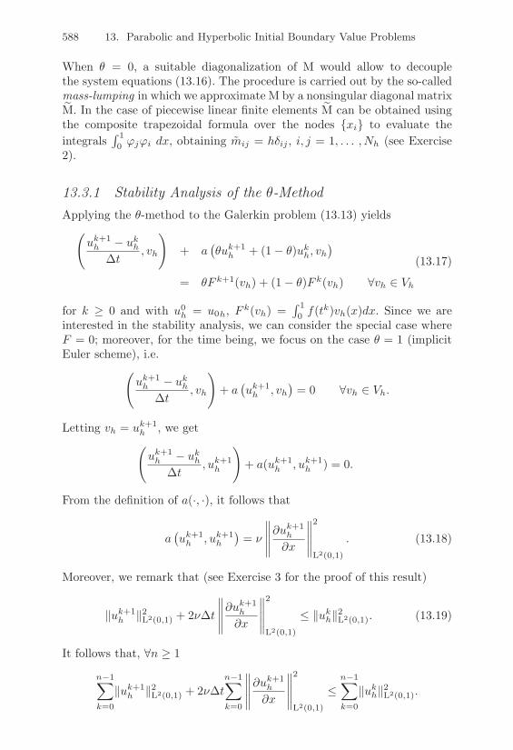
588 13. Parabolic and Hyperbolic Initial Boundary Value Problems
When ! = 0, a suitable diagonalization of M would allow to decouplethe system equations (13.16). The procedure is carried out by the so-calledmass-lumping in which we approximate M by a nonsingular diagonal matrixDM. In the case of piecewise linear finite elements DM can be obtained usingthe composite trapezoidal formula over the nodes {xi} to evaluate theintegrals
@ 10 1j1i dx, obtaining mij = h%ij , i, j = 1, . . . , Nh (see Exercise
2).
13.3.1 Stability Analysis of the !-MethodApplying the !-method to the Galerkin problem (13.13) yields
6uk+1h " uk
h
#t, vh
7
+ a8!uk+1
h + (1" !)ukh, vh
9
= !F k+1(vh) + (1" !)F k(vh) #vh ! Vh
(13.17)
for k ) 0 and with u0h = u0h, F k(vh) =
@ 10 f(tk)vh(x)dx. Since we are
interested in the stability analysis, we can consider the special case whereF = 0; moreover, for the time being, we focus on the case ! = 1 (implicitEuler scheme), i.e.
6uk+1h " uk
h
#t, vh
7
+ a8uk+1h , vh
9= 0 #vh ! Vh.
Letting vh = uk+1h , we get6uk+1h " uk
h
#t, uk+1
h
7
+ a(uk+1h , uk+1
h ) = 0.
From the definition of a(·, ·), it follows that
a8uk+1h , uk+1
h
9= 3
AAAAA.uk+1
h
.x
AAAAA
2
L2(0,1)
. (13.18)
Moreover, we remark that (see Exercise 3 for the proof of this result)
+uk+1h +2L2(0,1) + 23#t
AAAAA.uk+1
h
.x
AAAAA
2
L2(0,1)
& +ukh+2L2(0,1). (13.19)
It follows that, #n ) 1
n"1(
k=0
+uk+1h +2L2(0,1) + 23#t
n"1(
k=0
AAAAA.uk+1
h
.x
AAAAA
2
L2(0,1)
&n"1(
k=0
+ukh+2L2(0,1).
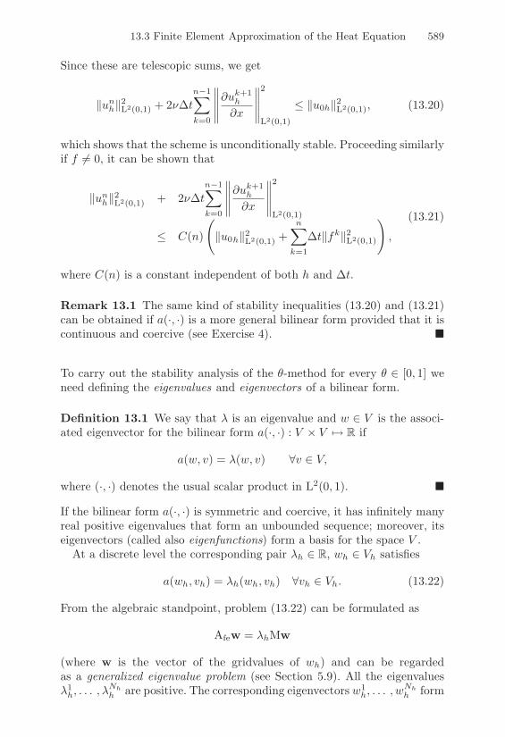
13.3 Finite Element Approximation of the Heat Equation 589
Since these are telescopic sums, we get
+unh+2L2(0,1) + 23#t
n"1(
k=0
AAAAA.uk+1
h
.x
AAAAA
2
L2(0,1)
& +u0h+2L2(0,1), (13.20)
which shows that the scheme is unconditionally stable. Proceeding similarlyif f '= 0, it can be shown that
+unh+2L2(0,1) + 23#t
n"1(
k=0
AAAAA.uk+1
h
.x
AAAAA
2
L2(0,1)
& C(n)
6
+u0h+2L2(0,1) +n(
k=1
#t+fk+2L2(0,1)
7
,
(13.21)
where C(n) is a constant independent of both h and #t.
Remark 13.1 The same kind of stability inequalities (13.20) and (13.21)can be obtained if a(·, ·) is a more general bilinear form provided that it iscontinuous and coercive (see Exercise 4). !
To carry out the stability analysis of the !-method for every ! ! [0, 1] weneed defining the eigenvalues and eigenvectors of a bilinear form.
Definition 13.1 We say that $ is an eigenvalue and w ! V is the associ-ated eigenvector for the bilinear form a(·, ·) : V % V D( R if
a(w, v) = $(w, v) #v ! V,
where (·, ·) denotes the usual scalar product in L2(0, 1). !
If the bilinear form a(·, ·) is symmetric and coercive, it has infinitely manyreal positive eigenvalues that form an unbounded sequence; moreover, itseigenvectors (called also eigenfunctions) form a basis for the space V .
At a discrete level the corresponding pair $h ! R, wh ! Vh satisfies
a(wh, vh) = $h(wh, vh) #vh ! Vh. (13.22)
From the algebraic standpoint, problem (13.22) can be formulated as
Afew = $hMw
(where w is the vector of the gridvalues of wh) and can be regardedas a generalized eigenvalue problem (see Section 5.9). All the eigenvalues$1h, . . . ,$
Nhh are positive. The corresponding eigenvectors w1
h, . . . , wNhh form

590 13. Parabolic and Hyperbolic Initial Boundary Value Problems
a basis for the subspace Vh and can be chosen in such a way as to be or-thonormal, i.e., such that (wi
h, wjh) = %ij , #i, j = 1, . . . , Nh. In particular,
any function vh ! Vh can be represented as
vh(x) =Nh(
j=1
vjwjh(x).
Let us now assume that ! ! [0, 1] and focus on the case where the bilinearform a(·, ·) is symmetric. Although the final stability result still holds inthe nonsymmetric case, the proof that follows cannot apply since in thatcase the eigenvectors would no longer form a basis for Vh. Let
/wi
h
0be the
eigenvectors of a(·, ·) whose span forms an orthonormal basis for Vh. Sinceat each time step uk
h ! Vh, we can express ukh as
ukh(x) =
Nh(
j=1
ukjw
jh(x).
Letting F = 0 in (13.17) and taking vh = wih, we find
1#t
Nh(
j=1
Puk+1j " uk
j
Q Kwj
h, wih
L
+Nh(
j=1
P!uk+1
j + (1" !)ukj
Qa(wj
h, wih) = 0, i = 1, . . . , Nh.
Since wjh are eigenfunctions of a(·, ·) we obtain
a(wjh, w
ih) = $jh(wj
h, wih) = $jh%ij = $ih,
so thatuk+1i " uk
i
#t+
P!uk+1
i + (1" !)uki
Q$ih = 0.
Solving this equation with respect to uk+1i gives
uk+1i = uk
i
P1" (1" !)$ih#t
QP1 + !$ih#t
Q .
In order for the method to be unconditionally stable we must have (seeChapter 11) >>>>
1" (1" !)$ih#t
1 + !$ih#t
>>>> < 1,
that is2! " 1 > " 2
$ih#t.
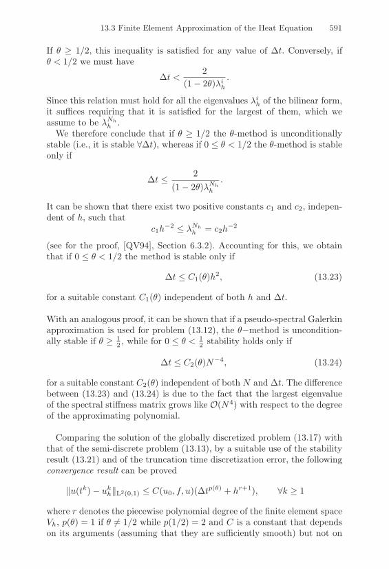
13.3 Finite Element Approximation of the Heat Equation 591
If ! ) 1/2, this inequality is satisfied for any value of #t. Conversely, if! < 1/2 we must have
#t <2
(1" 2!)$ih.
Since this relation must hold for all the eigenvalues $ih of the bilinear form,it su"ces requiring that it is satisfied for the largest of them, which weassume to be $Nh
h .We therefore conclude that if ! ) 1/2 the !-method is unconditionally
stable (i.e., it is stable ##t), whereas if 0 & ! < 1/2 the !-method is stableonly if
#t & 2(1" 2!)$Nh
h
.
It can be shown that there exist two positive constants c1 and c2, indepen-dent of h, such that
c1h"2 & $Nh
h = c2h"2
(see for the proof, [QV94], Section 6.3.2). Accounting for this, we obtainthat if 0 & ! < 1/2 the method is stable only if
#t & C1(!)h2, (13.23)
for a suitable constant C1(!) independent of both h and #t.
With an analogous proof, it can be shown that if a pseudo-spectral Galerkinapproximation is used for problem (13.12), the !"method is uncondition-ally stable if ! ) 1
2 , while for 0 & ! < 12 stability holds only if
#t & C2(!)N"4, (13.24)
for a suitable constant C2(!) independent of both N and #t. The di!erencebetween (13.23) and (13.24) is due to the fact that the largest eigenvalueof the spectral sti!ness matrix grows like O(N4) with respect to the degreeof the approximating polynomial.
Comparing the solution of the globally discretized problem (13.17) withthat of the semi-discrete problem (13.13), by a suitable use of the stabilityresult (13.21) and of the truncation time discretization error, the followingconvergence result can be proved
+u(tk)" ukh+L2(0,1) & C(u0, f, u)(#tp(() + hr+1), #k ) 1
where r denotes the piecewise polynomial degree of the finite element spaceVh, p(!) = 1 if ! '= 1/2 while p(1/2) = 2 and C is a constant that dependson its arguments (assuming that they are su"ciently smooth) but not on

592 13. Parabolic and Hyperbolic Initial Boundary Value Problems
h and #t. In particular, if f ? 0 on can obtain the following improvedestimates
+u(tk)" ukh+L2(0,1) & C
N4h/tk
5r+1
+4#t
tk
5p(()O
+u0+L2(0,1),
for k ) 1, ! = 1 or ! = 1/2. (For the proof of these results, see [QV94], pp.394-395).
Program 100 provides an implementation of the !-method for the solutionof the heat equation on the space-time domain (a, b) % (t0, T ). The dis-cretization in space is based on piecewise-linear finite elements. The inputparameters are: the column vector I containing the endpoints of the spaceinterval (a = I(1), b = I(2)) and of the time interval (t0 = I(3), T = I(4));the column vector n containing the number of steps in space and time; themacros u0 and f containing the functions u0h and f , the constant viscositynu, the Dirichlet boundary conditions bc(1) and bc(2), and the value ofthe parameter theta.
Program 100 - thetameth : !-method for the heat equation
function [u,x] = thetameth(I,n,u0,f,bc,nu,theta)nx = n(1); h = (I(2)-I(1))/nx;x = [I(1):h:I(2)]; t = I(3); uold = (eval(u0))’;nt = n(2); k = (I(4)-I(3))/nt; e = ones(nx+1,1);K = spdiags([(h/(6*k)-nu*theta/h)*e, (2*h/(3*k)+2*nu*theta/h)*e, ...
(h/(6*k)-nu*theta/h)*e],-1:1,nx+1,nx+1);B = spdiags([(h/(6*k)+nu*(1-theta)/h)*e, (2*h/(3*k)-nu*2*(1-theta)/h)*e, ...
(h/(6*k)+nu*(1-theta)/h)*e],-1:1,nx+1,nx+1);K(1,1) = 1; K(1,2) = 0; B(1,1) = 0; B(1,2) = 0;K(nx+1,nx+1) = 1; K(nx+1,nx) = 0; B(nx+1,nx+1) = 0; B(nx+1,nx) = 0;[L,U]=lu(K);t = I(3); x=[I(1)+h:h:I(2)-h]; fold = (eval(f))’;fold = h*fold;fold = [bc(1); fold; bc(2)];for time = I(3)+k:k:I(4)
t = time; fnew = (eval(f))’;fnew = h*fnew;fnew = [bc(1); fnew; bc(2)];b = theta*fnew+(1-theta)*fold + B*uold;y = L \ b; u = U \ y;uold = u;
endx = [I(1):h:I(2)];
Example 13.1 Let us assess the time-accuracy of the .-method in the solutionof the heat equation (13.1) on the space-time domain (0, 1) 1 (0, 1) where f is

13.4 Space-Time Finite Element Methods for the Heat Equation 593
chosen in such a way that the exact solution is u = sin(2+x) cos(2+t). A fixedspatial grid size h = 1/500 has been used while the time step $t is equal to(10k)%1, k = 1, . . . , 4. Finally, piecewise finite elements are used for the spacediscretization. Figure 13.1 shows the convergence behavior in the L2(0, 1) norm(evaluated at time t = 1), as $t tends to zero, of the backward Euler method(BE) (. = 1, solid line) and of the Crank-Nicolson scheme (CN) (. = 1/2, dashedline). As expected, the CN method is far more accurate than the BE method. •
101
102
10!7
10!6
10!5
10!4
10!3
10!2
10!1
FIGURE 13.1. Convergence analysis of the .-method as a function of the number1/$t of time steps (represented on the x-axis): . = 1 (solid line) and . = 0.5(dashed line)
13.4 Space-Time Finite Element Methods for theHeat Equation
An alternative approach for time discretization is based on the use of aGalerkin method to discretize both space and time variables.
Suppose to solve the heat equation for x ! [0, 1] and t ! [0, T ]. Let usdenote by Ik = [tk"1, tk] the k-th time interval for k = 1, . . . , n with #tk =tk" tk"1; moreover, we let #t = maxk#tk; the rectangle Sk = [0, 1]% Ik isthe so called space-time slab. At each time level tk, we consider a partitionThk of (0, 1) into mk subintervals Kk
j = [xkj , x
kj+1], j = 0, . . . ,mk " 1. We
let hkj = xk
j+1 " xkj and denote by hk = maxj hk
j and by h = maxk hk.Let us now associate with Sk a space-time partition Sk = 2mk
j=1Rkj where
Rkj = Kk
j % Ik and Kkj ! Thk . The space-time slab Sk is thus decomposed
into rectangles Rkj (see Figure 13.2).
For each time slab Sk we introduce the space-time finite element space
Qq(Sk) =Rv ! C0(Sk), v|Rk
j! P1(Kk
j )% Pq(Ik), j = 0, . . . ,mk " 1S

594 13. Parabolic and Hyperbolic Initial Boundary Value Problems
tk!1Rj
k Sk
t
0 1 x
tk
FIGURE 13.2. Space-time finite element discretization
where, usually, q = 0 or q = 1. Then, the space-time finite element spaceover [0, 1]% [0, T ] is defined as follows
Vh,!t =/v : [0, 1]% [0, T ] ( R : v|Sk
! Yh,k, k = 1, . . . , n0,
where
Yh,k = {v ! Qq(Sk) : v(0, t) = v(1, t) = 0 #t ! Ik} .
The number of degrees of freedom of Vh,!t is equal to (q + 1)(mk " 1).The functions in Vh,!t are linear and continuous in space while they arepiecewise polynomials of degree q in time. These functions are in generaldiscontinuous across the time levels tk and the partitions T k
h do not matchat the interface between contiguous time levels (see Figure 13.2). For thisreason, we adopt henceforth the following notation
vk± = lim/&0
v(tk ± 5), [vk] = vk+ " vk".
The discretization of problem (13.12) using continuous finite elements inspace of degree 1 and discontinuous finite elements of degree q in time(abbreviated by cG(1)dG(q) method) is: find U ! Vh,!t such that
n(
k=1
^
Ik
-4.U
.t, V
5+ a(U, V )
.dt +
n"1(
k=1
([Uk], V k+)
+(U0+, V
0+) =
T
0
(f, V ) dt, #V !0V h,!t,
where0V h,!t = {v ! Vh,!t : v(0, t) = v(1, t) = 0 #t ! [0, T ]} ,

13.4 Space-Time Finite Element Methods for the Heat Equation 595
U0" = u0h, Uk = U(x, tk) and (u, v) =
@ 10 uv dx denotes the scalar product
of L2(0, 1). The continuity of U at each point tk is therefore imposed onlyin a weak sense.
To construct the algebraic equations for the unknown U we need expand-ing it over a basis in time and in space. The single space-time basis func-tion 1k
jl(x, t) can be written as 1kjl(x, t) = 1k
j (x)6l(t), j = 1, . . . ,mk " 1,l = 0, . . . , q, where 1k
j is the usual piecewise linear basis function and 6l isthe l-th basis function of Pq(Ik).
When q = 0 the solution U is piecewise constant in time. In that case
Uk(x, t) =Nk
h(
j=1
Ukj 1
kj (x), x ! [0, 1], t ! Ik,
where Ukj = Uk(xj , t) #t ! Ik. Let
Ak = (aij) = (a(1kj ,1
ki )), Mk = (mij) = ((1k
j ,1ki )),
fk = (fi) =
G
H^
Sk
f(x, t)1ki (x)dx dt
I
J , Bk,k"1 = (bij) = ((1kj ,1
k"1i )),
denote the sti!ness matrix, the mass matrix, the data vector and the pro-jection matrix between V k"1
h and V kh , respectively, at the time level tk.
Then, letting Uk = (Ukj ), at each k-th time level the cG(1)dG(0) method
requires solving the following linear system8Mk +#tkAk
9Uk = Bk,k"1Uk"1 + fk,
which is nothing else than the Euler backward discretization scheme witha modified right hand side.
When q = 1, the solution is piecewise linear in time. For ease of notationwe let Uk(x) = U"(x, tk) and Uk"1(x) = U+(x, tk"1). Moreover, we assumethat the spatial partition Thk does not change with the time level and welet mk = m for every k = 0, . . . , n. Then, we can write
U|Sk= Uk"1(x)
tk " t
#tk+ Uk(x)
t" tk"1
#tk.
Thus the cG(1)dG(1) method leads to the solution of the following 2 %2 block-system in the unknowns Uk = (Uk
i ) and Uk"1 = (Uk"1i ), i =
1, . . . ,m" 1)**+
**,
4"1
2Mk +
#tk
3Ak
5Uk"1 +
412Mk +
#tk
6Ak
5Uk = fk"1 + Bk,k"1Uk"1
" ,4
12Mk +
#tk
6Ak
5Uk"1 +
412Mk +
#tk
3Ak
5Uk = fk

596 13. Parabolic and Hyperbolic Initial Boundary Value Problems
where
fk"1 =^
Sk
f(x, t)1ki (x)6k
1 (t)dx dt, fk =^
Sk
f(x, t)1ki (x)6k
2 (t)dx dt
and 6k1 (t) = (tk " t)/#tk, 6k
2 (t)(t" tk"1)/#tk are the two basis functionsof P1(Ik).
Assuming that Vh,k"1 '* Vh,k, it is possible to prove that (see for theproof [EEHJ96])
+u(tn)" Un+L2(0,1) & C(u0h, f, u, n)(#t2 + h2), (13.25)
where C is a constant that depends on its arguments (assuming that theyare su"ciently smooth) but not on h and #t.
An advantage in using space-time finite elements is the possibility toperform a space-time grid adaptivity on each time-slab based on a posteriorierror estimates (the interested reader is referred to [EEHJ96] where theanalysis of this method is carried out in detail).
Program 101 provides an implementation of the dG(1)cG(1) method forthe solution of the heat equation on the space-time domain (a, b)% (t0, T ).The input parameters are the same as in Program 100.
Program 101 - pardg1cg1 : dG(1)cG(1) method for the heat equation
function [u,x]=pardg1cg1(I,n,u0,f,nu,bc)nx = n(1); h = (I(2)-I(1))/nx;x = [I(1):h:I(2)]; t = I(3); um = (eval(u0))’;nt = n(2); k = (I(4)-I(3))/nt;e = ones(nx+1,1);Add = spdiags([(h/12-k*nu/(3*h))*e, (h/3+2*k*nu/(3*h))*e, ...
(h/12-k*nu/(3*h))*e],-1:1,nx+1,nx+1);Aud = spdiags([(h/12-k*nu/(6*h))*e, (h/3+k*nu/(3*h))*e, ...
(h/12-k*nu/(6*h))*e],-1:1,nx+1,nx+1);Ald = spdiags([(-h/12-k*nu/(6*h))*e, (-h/3+k*nu/(3*h))*e, ...
(-h/12-k*nu/(6*h))*e],-1:1,nx+1,nx+1);B = spdiags([h*e/6, 2*h*e/3, h*e/6],-1:1,nx+1,nx+1);Add(1,1) = 1; Add(1,2) = 0; B(1,1) = 0; B(1,2) = 0;Aud(1,1) = 0; Aud(1,2) = 0; Ald(1,1) = 0; Ald(1,2) = 0;Add(nx+1,nx+1)=1; Add(nx+1,nx)=0;B(nx+1,nx+1)=0; B(nx+1,nx) = 0;Ald(nx+1,nx+1)=0; Ald(nx+1,nx)=0;Aud(nx+1,nx+1)=0; Aud(nx+1,nx)=0;[L,U]=lu([Add Aud; Ald Add]);x = [I(1)+h:h:I(2)-h]; xx=[I(1),x,I(2)];for time = I(3)+k:k:I(4)

13.5 Hyperbolic Equations: A Scalar Transport Problem 597
t = time; fq1 = 0.5*k*h*eval(f);t = time-k; fq0 = 0.5*k*h*eval(f);rhs0 = [bc(1), fq0, bc(2)]; rhs1 = [bc(1), fq1, bc(2)];b = [rhs0’; rhs1’] + [B*um; zeros(nx+1,1)];y = L \ b; u = U \ y; um = u(nx+2:2*nx+2,1);
endx = [I(1):h:I(2)]; u = um;
Example 13.2 We assess the accuracy of the dG(1)cG(1) method on the sametest problem considered in Example 13.1. In order to neatly identify both spatialand temporal contributions in the error estimate (13.25) we have performed thenumerical computations using Program 101 by varying either the time step orthe space discretization step only, having chosen in each case the discretizationstep in the other variable su!ciently small that the corresponding error can beneglected. The convergence behavior in Figure 13.3 shows perfect agreement withthe theoretical results (second-order accuracy in both space and time). •
101
102
103
10!5
10!4
10!3
10!2
10!1
FIGURE 13.3. Convergence analysis for the dG(1)cG(1) method. The solid lineis the time discretization error while the dashed line is the space discretizationerror. In the first case the x-axis denotes the number of time steps while in secondcase it represents the number of space subintervals
13.5 Hyperbolic Equations: A Scalar TransportProblem
Let us consider the following scalar hyperbolic problem)+
,
.u
.t+ a
.u
.x= 0 x ! R, t > 0,
u(x, 0) = u0(x) x ! R,(13.26)

598 13. Parabolic and Hyperbolic Initial Boundary Value Problems
where a is a positive real number. Its solution is given by
u(x, t) = u0(x" at) t ) 0,
and represents a travelling wave with velocity a. The curves (x(t), t) in theplane (x, t), that satisfy the following scalar ordinary di!erential equation
)+
,
dx(t)dt
= a t > 0
x(0) = x0,(13.27)
are called characteristic curves. They are the straight lines x(t) = x0 + at,t > 0. The solution of (13.26) remains constant along them since
du
dt=.u
.t+.u
.x
dx
dt= 0 on (x(t), t).
For the more general problem)+
,
.u
.t+ a
.u
.x+ a0u = f x ! R, t > 0,
u(x, 0) = u0(x) x ! R,(13.28)
where a, a0 and f are given functions of the variables (x, t), the charac-teristic curves are still defined as in (13.27). In this case, the solutions of(13.28) satisfy along the characteristics the following di!erential equation
du
dt= f " a0u on (x(t), t).
P0
Q
P
#$x
t
t
x
t
t = 1
10
FIGURE 13.4. Left: examples of characteristics which are straight lines issuingfrom the points P and Q. Right: characteristic straight lines for the Burgersequation
Let us now consider problem (13.26) on a bounded interval. For example,assume that x ! [",#] and a > 0. Since u is constant along the character-istics, from Figure 13.4 (left) we deduce that the value of the solution at P

13.6 Systems of Linear Hyperbolic Equations 599
attains the value of u0 at P0, the foot of the characteristic issuing from P .On the other hand, the characteristic issuing from Q intersects the straightline x(t) = " at a certain time t = t > 0. Thus, the point x = " is aninflow point and it is necessary to assign a boundary value for u at x = "for every t > 0. Notice that if a < 0 then the inflow point is x = #.
Referring to problem (13.26) it is worth noting that if u0 is discontinuousat a point x0, then such a discontinuity propagates along the characteristicsissuing from x0. This process can be rigorously formalized by introducingthe concept of weak solutions of hyperbolic problems, see e.g. [GR96]. An-other reason for introducing weak solutions is that in the case of nonlinearhyperbolic problems the characteristic lines can intersect: in this case thesolution cannot be continuous and no classical solution does exist.
Example 13.3 (Burgers equation) Let us consider the Burgers equation
1u1t
+ u1u1x
= 0 x / R (13.29)
which is perhaps the simplest nontrivial example of a nonlinear hyperbolic equa-tion. Taking as initial condition
u(x, 0) = u0(x) =
)+
,
1 x " 0,1% x 0 " x " 1,0 x ! 1,
the characteristic line issuing from the point (x0, 0) is given by
x(t) = x0 + tu0(x0) =
)+
,
x0 + t x0 " 0,x0 + t(1% x0) 0 " x0 " 1,x0 x0 ! 1.
Notice that the characteristic lines do not intersect only if t < 1 (see Figure 13.4,right). •
13.6 Systems of Linear Hyperbolic Equations
Consider the linear hyperbolic systems of the form
.u.t
+ A.u.x
= 0 x ! R, t > 0, (13.30)
where u : R % [0,,) ( Rp and A ! Rp!p is a matrix with constantcoe"cients.
This system is said hyperbolic if A is diagonalizable and has real eigen-values, that is, if there exists a nonsingular matrix T ! Rp!p such that
A = T%T"1,

600 13. Parabolic and Hyperbolic Initial Boundary Value Problems
where % = diag($1, ...,$p) is the diagonal matrix of the real eigenvalues ofA, while T = (+1,+2, . . . ,+p) is the matrix whose column vectors are theright eigenvectors of A (see Section 1.7). The system is said to be strictlyhyperbolic if it is hyperbolic with distinct eigenvalues. Thus
A+k = $k+k, k = 1, . . . , p.
Introducing the characteristic variables w = T"1u, system (13.30) becomes
.w.t
+ %.w.x
= 0.
This is a system of p independent scalar equations of the form
.wk
.t+ $k
.wk
.x= 0, k = 1, . . . , p.
Proceeding as in Section 13.5 we obtain wk(x, t) = wk(x"$kt, 0), and thusthe solution u = Tw of problem (13.30) can be written as
u(x, t) =p(
k=1
wk(x" $kt, 0)+k.
The curve (xk(t), t) in the plane (x, t) that satisfies x*k(t) = $k is the k-th
characteristic curve and wk is constant along it. A strictly hyperbolic sys-tem enjoys the property that p distinct characteristic curves pass throughany point of the plane (x, t), for any fixed x and t. Then u(x, t) dependsonly on the initial datum at the points x"$kt. For this reason, the set of ppoints that form the feet of the characteristics issuing from the point (x, t)
D(t, x) =/x ! R : x = x" $kt , k = 1, ..., p
0, (13.31)
is called the domain of dependence of the solution u(x, t).If (13.30) is set on a bounded interval (",#) instead of on the whole real
line, the inflow point for each characteristic variable wk is determined by thesign of $k. Correspondingly, the number of positive eigenvalues determinesthe number of boundary conditions that can be assigned at x = ", whereasat x = # it is admissible to assign a number of conditions which equals thenumber of negative eigenvalues. An example is discussed in Section 13.6.1.
Remark 13.2 (The nonlinear case) Let us consider the following non-linear system of first-order equations
.u.t
+.
.xg(u) = 0 (13.32)
where g = (g1, . . . , gp)T is called the flux function. The system is hyperbolicif the jacobian matrix A(u) whose elements are aij = .gi(u)/.uj , i, j =1, . . . , p, is diagonalizable and has p real eigenvalues. !

13.6 Systems of Linear Hyperbolic Equations 601
13.6.1 The Wave EquationConsider the second-order hyperbolic equation
.2u
.t2" '2 .
2u
.x2 = f x ! (",#), t > 0, (13.33)
with initial data
u(x, 0) = u0(x) and.u
.t(x, 0) = v0(x), x ! (",#),
and boundary data
u(", t) = 0 and u(#, t) = 0, t > 0. (13.34)
In this case, u may represent the transverse displacement of an elasticvibrating string of length #"", fixed at the endpoints, and ' is a coe"cientdepending on the specific mass of the string and on its tension. The stringis subject to a vertical force of density f .
The functions u0(x) and v0(x) denote respectively the initial displace-ment and the initial velocity of the string.The change of variables
01 =.u
.x, 02 =
.u
.t,
transforms (13.33) into the following first-order system
.+
.t+ A
.+
.x= 0 x ! (",#), t > 0, (13.35)
where
+ =-0102
., A =
-0 "1"'2 0
.,
and the initial conditions are 01(x, 0) = u*0(x) and 02(x, 0) = v0(x).
Since the eigenvalues of A are the two distinct real numbers ±' (rep-resenting the propagation velocities of the wave) we conclude that system(13.35) is hyperbolic. Moreover, one boundary condition needs to be pre-scribed at every end-point, as in (13.34). Notice that, also in this case,smooth solutions correspond to smooth initial data, while any discontinuitythat is present in the initial data will propagate along the characteristics.
Remark 13.3 Notice that replacing )2u)t2 by t2, )2u
)x2 by x2 and f by 1, thewave equation becomes
t2 " '2x2 = 1

602 13. Parabolic and Hyperbolic Initial Boundary Value Problems
which represents an hyperbola in the (x, t) plane. Proceeding analogouslyin the case of the heat equation (13.1), we end up with
t" 3x2 = 1
which represents a parabola in the (x, t) plane. Finally, for the Poissonequation (12.90), replacing )2u
)x2 by x2, )2u)y2 by y2 and f by 1, we get
x2 + y2 = 1
which represents an ellipse in the (x, y) plane.Due to the geometric interpretation above, the corresponding di!erential
operators are classified as hyperbolic, parabolic and elliptic. !
13.7 The Finite Di"erence Method for HyperbolicEquations
Let us discretize the hyperbolic problem (13.26) by space-time finite dif-ferences. To this aim, the half-plane {(x, t) : ", < x <,, t > 0} is dis-cretized by choosing a spatial grid size #x, a temporal step #t and thegrid points (xj , tn) as follows
xj = j#x, j ! Z, tn = n#t, n ! N.
Let us set$ = #t/#x,
and define xj+1/2 = xj + #x/2. We look for discrete solutions unj which
approximate the values u(xj , tn) of the exact solution for any j, n.Quite often, explicit methods are employed for advancing in time in
hyperbolic initial-value problems, even though they require restrictions onthe value of $, unlike what typically happens with implicit methods.Let us focus our attention on problem (13.26). Any explicit finite-di!erencemethod can be written in the form
un+1j = un
j " $(hnj+1/2 " hn
j"1/2), (13.36)
where hnj+1/2 = h(un
j , unj+1) for every j and h(·, ·) is a particular function
that is called the numerical flux.
13.7.1 Discretization of the Scalar EquationWe illustrate several instances of explicit methods, and provide the corre-sponding numerical flux.

13.7 The Finite Di"erence Method for Hyperbolic Equations 603
1. Forward Euler/centred
un+1j = un
j "$
2a(un
j+1 " unj"1) (13.37)
which can be cast in the form (13.36) by setting
hj+1/2 =12a(uj+1 + uj). (13.38)
2. Lax-Friedrichs
un+1j =
12(un
j+1 + unj"1)"
$
2a(un
j+1 " unj"1) (13.39)
which is of the form (13.36) with
hj+1/2 =12[a(uj+1 + uj)" $"1(uj+1 " uj)].
3. Lax-Wendro!
un+1j = un
j "$
2a(un
j+1 " unj"1) +
$2
2a2(un
j+1 " 2unj + un
j"1) (13.40)
which can be written in the form (13.36) provided that
hj+1/2 =12[a(uj+1 + uj)" $a2(uj+1 " uj)].
4. Upwind (or forward Euler/uncentred)
un+1j = un
j "$
2a(un
j+1 " unj"1) +
$
2|a|(un
j+1 " 2unj + un
j"1) (13.41)
which fits the form (13.36) when the numerical flux is defined to be
hj+1/2 =12[a(uj+1 + uj)" |a|(uj+1 " uj)].
The last three methods can be obtained from the forward Euler/centredmethod by adding a term proportional to a numerical di!usion, so thatthey can be written in the equivalent form
un+1j = un
j "$
2a(un
j+1 " unj"1) +
12kunj+1 " 2un
j + unj"1
(#x)2, (13.42)
where the artificial viscosity k is given for the three cases in Table 13.1.

604 13. Parabolic and Hyperbolic Initial Boundary Value Problems
methods k hdiffj+1/2 5(#t,#x)
Lax-Friedrichs #x2 " 12$
(uj+1 " uj) O4#x2
#t+#t +#x
5
Lax-Wendro! a2#t2 "$a2
2(uj+1 " uj) O
8#t2 +#x29
Upwind |a|#x#t " |a|2
(uj+1 " uj) O(#t +#x)
TABLE 13.1. Artificial viscosity, artificial flux and truncation error forLax-Friedrichs, Lax-Wendro" and Upwind methods
As a consequence, the numerical flux for each scheme can be written equiv-alently as
hj+1/2 = hFEj+1/2 + hdiff
j+1/2
where hFEj+1/2 is the numerical flux of the forward Euler/centred scheme
(which is given in (13.38)) and the artificial di!usion flux hdiffj+1/2 is given
for the three cases in Table 13.1.
An example of an implicit method is the backward Euler/centred scheme
un+1j +
$
2a(un+1
j+1 " un+1j"1 ) = un
j . (13.43)
It can still be written in the form (13.36) provided that hn is replaced byhn+1. In the example at hand, the numerical flux is the same as for theForward Euler/centred method, and so is the artificial viscosity.
Finally, we report the following schemes for the approximation of thesecond-order wave equation (13.33):
1. Leap-Frog
un+1j " 2un
j + un"1j = ('$)2(un
j+1 " 2unj + un
j"1) (13.44)
2. Newmark
un+1j " un
j = #tvnj + ('$)2P#wn+1
j +8 1
2 " #9wn
j
Q,
vn+1j " vnj =
('$)2
#t
P!wn+1
j + (1" !)wnj
Q (13.45)
with wj = uj+1"2uj+uj"1 and where the parameters # and ! satisfy0 & # & 1
2 , 0 & ! & 1.
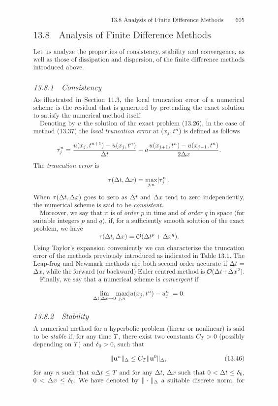
13.8 Analysis of Finite Di"erence Methods 605
13.8 Analysis of Finite Di"erence Methods
Let us analyze the properties of consistency, stability and convergence, aswell as those of dissipation and dispersion, of the finite di!erence methodsintroduced above.
13.8.1 ConsistencyAs illustrated in Section 11.3, the local truncation error of a numericalscheme is the residual that is generated by pretending the exact solutionto satisfy the numerical method itself.
Denoting by u the solution of the exact problem (13.26), in the case ofmethod (13.37) the local truncation error at (xj , tn) is defined as follows
5nj =u(xj , tn+1)" u(xj , tn)
#t" a
u(xj+1, tn)" u(xj"1, tn)2#x
.
The truncation error is
5(#t,#x) = maxj,n
|5nj |.
When 5(#t,#x) goes to zero as #t and #x tend to zero independently,the numerical scheme is said to be consistent.
Moreover, we say that it is of order p in time and of order q in space (forsuitable integers p and q), if, for a su"ciently smooth solution of the exactproblem, we have
5(#t,#x) = O(#tp +#xq).
Using Taylor’s expansion conveniently we can characterize the truncationerror of the methods previously introduced as indicated in Table 13.1. TheLeap-frog and Newmark methods are both second order accurate if #t =#x, while the forward (or backward) Euler centred method is O(#t+#x2).
Finally, we say that a numerical scheme is convergent if
lim!t,!x&0
maxj,n
|u(xj , tn)" un
j | = 0.
13.8.2 StabilityA numerical method for a hyperbolic problem (linear or nonlinear) is saidto be stable if, for any time T , there exist two constants CT > 0 (possiblydepending on T ) and %0 > 0, such that
+un+! & CT +u0+!, (13.46)
for any n such that n#t & T and for any #t, #x such that 0 < #t & %0,0 < #x & %0. We have denoted by + · +! a suitable discrete norm, for

606 13. Parabolic and Hyperbolic Initial Boundary Value Problems
instance one of those indicated below
+v+!,p =
G
H#x$(
j="$|vj |p
I
J
1p
p = 1, 2, +v+!,$ = supj|vj |. (13.47)
Note that +·+!,p is an approximation of the norm of Lp(R). For instance, theimplicit Bacward Euler/centred scheme (13.43) is unconditionally stablewith respect to the norm + · +!,2 (see Exercise 7).
13.8.3 The CFL ConditionCourant, Friedrichs and Lewy [CFL28] have shown that a necessary andsu"cient condition for any explicit scheme of the form (13.36) to be stableis that the time and space discretization steps must obey the followingcondition
|a$| =>>>>a#t
#x
>>>> & 1 (13.48)
which is known as the CFL condition. The number a$, which is an adi-mensional number since a is a velocity, is commonly referred to as the CFLnumber. If a is not constant the CFL condition becomes
#t & #x
supx#R, t>0
|a(x, t)| ,
while, in the case of the hyperbolic system (13.30), the stability conditionbecomes
>>>>$k#t
#x
>>>> & 1 k = 1, . . . , p,
where {$k : k = 1 . . . , p} are the eigenvalues of A.
The CFL stability condition has the following geometric interpretation.In a finite di!erence scheme the value un+1
j depends, in general, on thevalues of un at the three points xj+i, i = "1, 0, 1. Thus, at the time t = 0the solution un+1
j will depend only on the initial data at the points xj+i,for i = "(n + 1), . . . , (n + 1) (see Figure 13.5).
Let us define numerical domain of dependence D!t(xj , tn) to be the setof values at time t = 0 the numerical solution un
j depends on, that is
D!t(xj , tn) *
Ex ! R : |x" xj | & n#x =
tn
$
F.

13.8 Analysis of Finite Di"erence Methods 607
xj+(n+1)
t
tn+1
tn
xj"1xj"(n+1) xj xj+1
x
t1
t0
FIGURE 13.5. The numerical domain of dependence D#t(xj , tn+1)
Consequently, for any fixed point (x, t) we have
D!t(x, t) *Ex ! R : |x" x| & t
$
F.
In particular, taking the limit as#t( 0 for a fixed $, the numerical domainof dependence becomes
D0(x, t) =Ex ! R : |x" x| & t
$
F.
The condition (13.48) is thus equivalent to the inclusion
D(x, t) * D0(x, t), (13.49)
where D(x, t) is the domain of dependence defined in (13.31).In the case of an hyperbolic system, thanks to (13.49), we can conclude
that the CFL condition requires that any straight line x = x " $k(t " t),k = 1, . . . , p, must intersect the temporal straight line t = t"#t at somepoint x belonging to the domain of dependence (see Figure 13.6).
Let us analyze the stability properties of some of the methods introducedin the previous section.Assuming that a > 0, the upwind scheme (13.41) can be reformulated as
un+1j = un
j " $a(unj " un
j"1). (13.50)
Therefore
+un+1+!,1 & #x(
j
|(1" $a)unj | +#x
(
j
|$aunj"1|.

608 13. Parabolic and Hyperbolic Initial Boundary Value Problems
x +#x
t
(x, t)
x"#x x x +#x
(x, t)
r1 r2r2r1
t
t"#tx"#x x
FIGURE 13.6. Geometric interpretation of the CFL condition for a system withp = 2, where ri = x % #i(t % t) i = 1, 2. The CFL condition is satisfied for theleft-hand case, while it is violated for the right-hand case
Both $a and 1" $a are nonnegative if (13.48) holds. Thus
+un+1+!,1 & #x(1" $a)(
j
|unj | +#x$a
(
j
|unj"1| = +un+!,1.
Inequality (13.46) is therefore satisfied by taking CT = 1 and +·+! = +·+!,1.
The Lax-Friedrichs scheme is also stable, upon assuming (13.48). Indeed,from (13.39) we get
un+1j =
12(1" $a)un
j+1 +12(1 + $a)un
j"1.
Therefore,
+un+1+!,1 & 12#x
"
$
>>>>>>
(
j
(1" $a)unj+1
>>>>>>+
>>>>>>
(
j
(1 + $a)unj"1
>>>>>>
%
'
& 12(1" $a)+un+!,1 +
12(1 + $a)+un+!,1 = +un+!,1.
Also the Lax-Wendro! scheme is stable under the usual assumption (13.48)on #t (for the proof see, e.g., [QV94] Chapter 14).
13.8.4 Von Neumann Stability AnalysisLet us now show that the condition (13.48) is not su"cient to ensure thatthe forward Euler/centred scheme (13.37) is stable. For this purpose, wemake the assumption that the function u0(x) is 2&-periodic so that it canbe expanded in a Fourier series as
u0(x) =$(
k="$"ke
ikx (13.51)

13.8 Analysis of Finite Di"erence Methods 609
where
"k =12&
2"^
0
u0(x) e"ikx dx
is the k-th Fourier coe"cient of u0 (see Section 10.9). Therefore,
u0j = u0(xj) =
$(
k="$"ke
ikjh j = 0, ±1, ±2, · · ·
where we have set h = #x for ease of notation. Applying (13.37) with n = 0we get
u1j =
$(
k="$"ke
ikjh
41" a#t
2h(eikh " e"ikh)
5
=$(
k="$"ke
ikjh
41" a#t
hi sin(kh)
5.
Setting
'k = 1" a#t
hi sin(kh),
and proceeding recursively on n yields
unj =
$(
k="$"ke
ikjh'nk j = 0,±1,±2, . . . , n ) 1. (13.52)
The number 'k ! C is said to be the amplification coe"cient of the k-thfrequency (or harmonic) at each time step. Since
|'k| =
B
1 +4a#t
hsin(kh)
52C 1
2
,
we deduce that
|'k| > 1 if a '= 0 and k '= m&
h, m = 0,±1,±2, . . .
Correspondingly, the nodal values |unj | continue to grow as n(, and the
numerical solution ”blows-up” whereas the exact solution satisfies
|u(x, t)| = |u0(x" at)| & maxs#R
|u0(s)| #x ! R, #t > 0.
The centred discretization scheme (13.37) is thus unconditionally unstable,i.e., it is unstable for any choice of the parameters #t and #x.

610 13. Parabolic and Hyperbolic Initial Boundary Value Problems
The previous analysis is based on the Fourier series expansion and iscalled von Neumann analysis. It can be applied to studying the stability ofany numerical scheme with respect to the norm + ·+!,2 and for establishingthe dissipation and dispersion of the method.
Any explicit finite di!erence numerical scheme for problem (13.26) satis-fies a recursive relation analogous to (13.52), where 'k depends a priori on#t and h and is called the k-th amplification coe"cient of the numericalscheme at hand.
Theorem 13.1 Assume that for a suitable choice of #t and h, |'k| & 1#k; then, the numerical scheme is stable with respect to the + · +!,2 norm.
Proof. Take an initial datum with a finite Fourier expansion
u0(x) =
N2 %1(
k=%N2
$keikx
where N is a positive integer. Without loss of generality we can assume thatproblem (13.26) is well-posed on [0, 2+] since u0 is a 2+-periodic function. Takein this interval N equally spaced nodes
xj = jh j = 0, . . . , N % 1, with h =2+N
,
at which the numerical scheme (13.36) is applied. We get
u0j = u0(xj) =
N2 %1(
k=%N2
$keikjh, un
j =
N2 %1(
k=%N2
$k,nk e
ikjh.
Notice that
&un&2#,2 = hN%1(
j=0
N2 %1(
k,m=%N2
$k$m(,k,m)nei(k%m)jh.
Recalling Lemma 10.1 we have
hN%1(
j=0
ei(k%m)jh = 2+!km, %N2" k,m " N
2% 1,
which yields
&un&2#,2 = 2+
N2 %1(
k=%N2
|$k|2|,k|2n.
As a consequence, since |,k| " 1 )k, it turns out that
&un&2#,2 " 2+
N2 %1(
k=%N2
&$k&2 = &u0&2#,2, )n ! 0,
13.9 Dissipation and Dispersion 611
which proves that the scheme is stable with respect to the & · &#,2 norm. !
In the case of the upwind scheme (13.41), proceeding as was done forthe centred scheme, we find the following amplification coe"cients (seeExercise 6)
'k =
)*+
*,
1" a#t
h(1" e"ikh) if a > 0,
1" a#t
h(e"ikh " 1) if a < 0.
Therefore#k, |'k| & 1 if #t & h
|a| ,
which is nothing but the CFL condition.Thanks to Theorem 13.1, if the CFL condition is satisfied, the upwind
scheme is stable with respect to the + · +!,2 norm.We conclude by noting that the upwind scheme (13.50) satisfies
un+1j = (1" $a)un
j + $aunj"1.
Owing to (13.48), either $a or 1" $a are nonnegative, thus
min(unj , u
nj"1) & un+1
j & max(unj , u
nj"1).
It follows that
infl#Z
/u0l
0& un
j & supl#Z
/u0l
0#j ! Z, #n ) 0,
that is,
+un+!,$ & +u0+!,$ #n ) 0, (13.53)
which proves that if (13.48) is satisfied, the upwind scheme is stable in thenorm +·+!,$. The relation (13.53) is called the discrete maximum principle(see also Section 12.2.2).
Remark 13.4 For the approximation of the wave equation (13.33) theLeap-Frog method (13.44) is stable under the CFL restriction#t & #x/|'|,while the Newmark method (13.45) is unconditionally stable if 2# ) ! ) 1
2(see [Joh90]). !
13.9 Dissipation and Dispersion
The von Neumann analysis on the amplification coe"cients enlightens thestudy of the stability and dissipation of a numerical scheme.

612 13. Parabolic and Hyperbolic Initial Boundary Value Problems
Consider the exact solution to problem (13.26); the following relationholds
u(x, tn) = u0(x" an#t), #n ) 0, #x ! R.
In particular, from applying (13.51) it follows that
u(xj , tn) =
$(
k="$"ke
ikjhgnk , where gk = e"iak!t. (13.54)
Letting1k = k#x,
we have k#t = $1k and thus
gk = e"ia#1k . (13.55)
The real number 1k, here expressed in radians, is called the phase angle ofthe k-th harmonic. Comparing (13.54) with (13.52) we can see that 'k isthe counterpart of gk which is generated by the specific numerical methodat hand. Moreover, |gk| = 1, whereas |'k| & 1, in order to ensure stability.
Thus, 'k is a dissipation coe"cient; the smaller |'k|, the higher the reduc-tion of the amplitude "k, and, as a consequence, the higher the numericaldissipation.The ratio /a(k) = |-k|
|gk| is called the amplification error of the k-th harmonicassociated with the numerical scheme (in our case it coincides with theamplification coe"cient). On the other hand, writing
'k = |'k|e"i*!t = |'k|e"i0
k$1k
,
and comparing this relation with (13.55), we can identify the velocity ofpropagation of the numerical solution, relative to its k-th harmonic, asbeing *
k . The ratio between this velocity and the velocity a of the exactsolution is called the dispersion error /d relative to the k-th harmonic
/d(k) =0
ka=0#x
1ka.
The amplification and dispersion errors for the numerical schemes exam-ined so far are functions of the phase angle 1k and the CFL number a$.This is shown in Figure 13.7 where we have only considered the interval0 & 1k & & and we have used degrees instead of radians to denote thevalues of 1k.
In Figure 13.8 the numerical solutions of equation (13.26) with a = 1and the initial datum u0 given by a packet of two sinusoidal waves of equalwavelength l and centred at the origin x = 0 are shown. The plots on theleft-side of the figure refer to the case l = 10#x while on the right-side

13.9 Dissipation and Dispersion 613
0 20 40 60 80 100 120 140 160 180
0.2
0.4
0.6
0.8
1
Amplification error for Lax!Friedrichs
&
' a
0 20 40 60 80 100 120 140 160 180
1
2
3
4
5
Dispersion error for Lax!Friedrichs
&
' &
CFL= 0.25CFL= 0.50CFL= 0.75CFL= 1.00
CFL= 0.25CFL= 0.50CFL= 0.75CFL= 1.00
0 20 40 60 80 100 120 140 160 180
0
0.2
0.4
0.6
0.8
1
1.2Amplification error for Lax!Wendroff
&
' a
0 20 40 60 80 100 120 140 160 180
0
0.2
0.4
0.6
0.8
1
1.2
1.4
Dispersion error for Lax!Wendroff
&
' &
CFL= 0.25CFL= 0.50CFL= 0.75CFL= 1.00
CFL= 0.25CFL= 0.50CFL= 0.75CFL= 1.00
0 20 40 60 80 100 120 140 160 180!0.2
0
0.2
0.4
0.6
0.8
1
1.2
Amplification error for Upwind
&
' a
0 20 40 60 80 100 120 140 160 180
0
0.2
0.4
0.6
0.8
1
1.2
1.4
Dispersion error for Upwind
&
' &
CFL= 0.25CFL= 0.50CFL= 0.75CFL= 1.00
CFL= 0.25CFL= 0.50CFL= 0.75CFL= 1.00
FIGURE 13.7. Amplification and dispersion errors for several numerical schemes
we have l = 4#x. Since k = (2&)/l we get 1k = ((2&)/l)#x, so that1k = &/10 in the left-side pictures and 1k = &/4 in the right-side ones.All numerical solutions have been computed for a CFL number equal to0.75, using the schemes introduced above. Notice that the dissipation e!ectis quite relevant at high frequencies (1k = &/4), especially for first-ordermethods (such as the upwind and the Lax-Friedrichs methods).
In order to highlight the e!ects of the dispersion, the same computa-tions have been repeated for 1k = &/3 and di!erent values of the CFLnumber. The numerical solutions after 5 time steps are shown in Figure13.9. The Lax-Wendro! method is the least dissipative for all the consid-ered CFL numbers. Moreover, a comparison of the positions of the peaksof the numerical solutions with respect to the corresponding ones in the
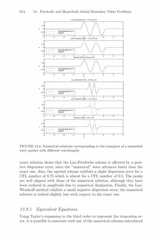
614 13. Parabolic and Hyperbolic Initial Boundary Value Problems
!4 !3 !2 !1 0 1 2 3 4!1
!0.5
0
0.5
1
xu
Lax!Wendroff CFL= 0.75 &=%/10
Computed at t=1Exact
!4 !3 !2 !1 0 1 2 3 4!1
!0.5
0
0.5
1
x
uLax!Friedrichs CFL= 0.75 &=%/10
Computed at t=1Exact
!4 !3 !2 !1 0 1 2 3 4!1
!0.5
0
0.5
1
x
u
Upwind CFL= 0.75 &=%/10
Computed at t=1Exact
!4 !3 !2 !1 0 1 2 3 4!1
!0.5
0
0.5
1
x
u
Lax!Wendroff CFL= 0.75 &=%/4
Computed at t=1Exact
!4 !3 !2 !1 0 1 2 3 4!1
!0.5
0
0.5
1
x
u
Lax!Friedrichs CFL= 0.75 &=%/4
Computed at t=1Exact
!4 !3 !2 !1 0 1 2 3 4!1
!0.5
0
0.5
1
x
u
Upwind CFL= 0.75 &=%/4
Computed at t=1Exact
FIGURE 13.8. Numerical solutions corresponding to the transport of a sinusoidalwave packet with di"erent wavelengths
exact solution shows that the Lax-Friedrichs scheme is a!ected by a posi-tive dispersion error, since the ”numerical” wave advances faster than theexact one. Also, the upwind scheme exhibits a slight dispersion error for aCFL number of 0.75 which is absent for a CFL number of 0.5. The peaksare well aligned with those of the numerical solution, although they havebeen reduced in amplitude due to numerical dissipation. Finally, the Lax-Wendro! method exhibits a small negative dispersion error; the numericalsolution is indeed slightly late with respect to the exact one.
13.9.1 Equivalent EquationsUsing Taylor’s expansion to the third order to represent the truncation er-ror, it is possible to associate with any of the numerical schemes introduced
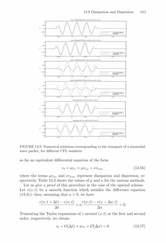
13.9 Dissipation and Dispersion 615
!1 !0.5 0 0.5 1 1.5 2!1
!0.5
0
0.5
1
uLax!Wendroff CFL=0.50 &=%/3, t=4( t
ComputedExact
!1 !0.5 0 0.5 1 1.5 2
!1
!0.5
0
0.5
1
u
Lax!Wendroff CFL=0.75 &=%/3, t=4( t
ComputedExact
!1 !0.5 0 0.5 1 1.5 2
!1
!0.5
0
0.5
1
u
Lax!Friedrichs CFL=0.50 &=%/3, t=5( t
ComputedExact
!1 !0.5 0 0.5 1 1.5 2!1
!0.5
0
0.5
1
u
Lax!Friedrichs CFL=0.75 &=%/3, t=5( t
ComputedExact
!1 !0.5 0 0.5 1 1.5 2
!1
!0.5
0
0.5
1
u
Upwind CFL=0.50 &=%/3, t=4( t
ComputedExact
!1 !0.5 0 0.5 1 1.5 2!1
!0.5
0
0.5
1
u
Upwind CFL=0.75 &=%/3, t=4( t
ComputedExact
FIGURE 13.9. Numerical solutions corresponding to the transport of a sinusoidalwave packet, for di"erent CFL numbers
so far an equivalent di!erential equation of the form
vt + avx = µvxx + 3vxxx (13.56)
where the terms µvxx and 3vxxx represent dissipation and dispersion, re-spectively. Table 13.2 shows the values of µ and 3 for the various methods.
Let us give a proof of this procedure in the case of the upwind scheme.Let v(x, t) be a smooth function which satisfies the di!erence equation(13.41); then, assuming that a > 0, we have
v(x, t +#t)" v(x, t)#t
+ av(x, t)" v(x"#x, t)
#x= 0.
Truncating the Taylor expansions of v around (x, t) at the first and secondorder, respectively, we obtain
vt + O(#t) + avx + O(#x) = 0 (13.57)

616 13. Parabolic and Hyperbolic Initial Boundary Value Problems
Method µ 3
Upwinda#x
2" a2#t
2"a
68#x2 " 3a#x#t + 2a2#t2
9
Lax-Friedrichs#x2
2#t
81" (a$)2
9 a#x2
381" (a$)2
9
Lax-Wendro! 0a#x2
68(a$)2 " 1
9
TABLE 13.2. Values of dissipation and dispersion coe!cients for several numer-ical methods
and
vt +#t
2vtt + O(#t2) + a
4vx +
#x
2vxx + O(#x2)
5= 0, (13.58)
where vt = )v)t and vx = )v
)x .Di!erentiating (13.57) with respect to t and then with respect to x, we
getvtt + avxt = O(#x +#t),
andvtx + avxx = O(#x +#t).
Thus, it follows that
vtt = a2vxx + O(#x +#t),
which, after substituting into (13.58), yields the following equation
vt + avx = µvxx (13.59)
whereµ =
a#x
2" a2#t
2,
and having neglected the term O(#x2+#t2). Relation (13.59) is the equiv-alent di!erential equation up to second order of the upwind scheme.
Following the same procedure and truncating the Taylor expansion atthird order, yields
vt + avx = µvxx + 3vxxx (13.60)
where3 =
a
68a2#t2 "#x29 .
We can give a heuristic explanation of the meaning of the dissipativeand dispersive terms in the equivalent equation (13.56) by studying thefollowing problem
Bvt + avx = µvxx + 3vxxx x ! R, t > 0
v(x, 0) = eikx, (k ! Z)(13.61)

13.9 Dissipation and Dispersion 617
Applying the Fourier transform yields, if µ = 3 = 0,
v(x, t) = eik(x"at), (13.62)
while if µ and 3 are arbitrary real numbers (with µ > 0) we get
v(x, t) = e"µk2teik[x"(a+.k2)t]. (13.63)
Comparing (13.62) with (13.63) we can see that the module of the solutiondiminishes as µ grows and this becomes more relevant if the frequency kgets larger. Therefore, the term µvxx in (13.61) has a dissipative e!ect onthe solution. A further comparison between (13.62) and (13.63) shows thatthe presence of the term 3 modifies the velocity of the propagation of thesolution; the velocity is increased if 3 > 0 whereas it is diminuished if 3 < 0.Even in this case the e!ect is amplified at high frequencies. Therefore, thethird-order di!erential term 3vxxx introduces a dispersive e!ect.
Generally speaking, even-order derivatives in the equivalent equation rep-resent di!usive terms, while odd-order derivatives mean dispersive e!ects.In the case of first-order schemes (like the upwind method) the dispersivee!ect is often only slightly visible since it is hidden by the dissipative one.Actually, taking #t and #x of the same order, we have that 3 << µ as#x ( 0, since 3 = O(#x2) and µ = O(#x). In particular, for a CFLnumber of 1
2 , the equivalent equation of the upwind method exhibits nulldispersion, truncated at second order, according to the results of the pre-vious section.
On the other hand, the dispersive e!ect is strikingly visible in the Lax-Friedrichs and in the Lax-Wendro! schemes; the latter, being second-orderaccurate, does not exhibit a dissipative term of the form µvxx. However,it ought to be dissipative in order to be stable; actually, the equivalentequation (truncated at fourth order) for the Lax-Wendro! scheme reads
vt + avx =a#x2
6[(a$)2 " 1]vxxx "
a#x3
6a$[1" (a$)2]vxxxx
where the last term is dissipative if |a$| < 1. We thus recover the CFLcondition for the Lax-Wendro! method.

618 13. Parabolic and Hyperbolic Initial Boundary Value Problems
13.10 Finite Element Approximation of HyperbolicEquations
Let us consider the following first-order linear, scalar hyperbolic problemin the interval ( = (",#) * R
)*****+
*****,
.u
.t+ a
.u
.x+ a0u = f in QT = (% (0, T )
u(", t) = 1(t) t ! (0, T )
u(x, 0) = u0(x) x ! (,
(13.64)
where a = a(x), a0 = a0(x, t), f = f(x, t), 1 = 1(t) and u0 = u0(x) aregiven functions.
We assume that a(x) > 0 #x ! [",#]. In particular, this implies thatthe point x = " is the inflow boundary, and the boundary value has to bespecified there.
13.10.1 Space Discretization with Continuous andDiscontinuous Finite Elements
A semi-discrete approximation of problem (13.64) can be carried out bymeans of the Galerkin method (see Section 12.4). Define the spaces
Vh = Xrh =
/vh ! C0(() : vh|Ij ! Pr(Ij), # Ij ! Th
0
andV inh = {vh ! Vh : vh(") = 0} ,
where Th is a partition of ( (see Section 12.4.5) into n ) 2 subintervalsIj = [xj , xj+1], for j = 0, . . . , n" 1.
Let u0,h be a suitable finite element approximation of u0 and considerthe problem: for any t ! (0, T ) find uh(t) ! Vh such that
)********+
********,
'
!
.uh(t).t
vh dx +
'
!
4a.uh(t).x
+ a0(t)uh(t)5vh dx
=
'
!
f(t)vh dx # vh ! V inh
uh(t) = 1h(t) at x = ",
(13.65)
with uh(0) = u0,h ! Vh.

13.10 Finite Element Approximation of Hyperbolic Equations 619
If 1 is equal to zero, uh(t) ! V inh , and we are allowed to taking vh = uh(t)
and get the following inequality
+uh(t)+2L2(!,') +t^
0
µ0+uh(5)+2L2(!,') d5 + a(#)t^
0
u2h(5) d5
& +u0,h+2L2(!,') +t^
0
1µ0+f(5)+2L2(!,')d5 ,
for any t ! [0, T ], where we have assumed that
0 < µ0 & a0(x, t)"12a*(x). (13.66)
Notice that in the special case in which both f and a0 are identically zero,we obtain
+uh(t)+L2(!,') & +u0,h+L2(!,')
which expresses the conservation of the energy of the system. When (13.66)does not hold (for example, if a is a constant convective term and a0 = 0),then an application of Gronwall’s lemma 11.1 yields
+uh(t)+2L2(!,') + a(#)t^
0
u2h(5) d5
&
G
H+u0,h+2L2(!,') +t^
0
+f(5)+2L2(!,') d5
I
J expt^
0
[1 + 2µ,(5)] d5,
(13.67)
where µ,(t) = max[!,']
|µ(x, t)|.
An alternative approach to the semi-discrete approximation of problem(13.64) is based on the use of discontinuous finite elements. This choiceis motivated by the fact that, as previously pointed out, the solutions ofhyperbolic problems (even in the linear case) may exhibit discontinuities.
The finite element space can be defined as follows
Wh = Y rh =
/vh ! L2(",#) : vh|Ij ! Pr(Ij), # Ij ! Th
0,
i.e., the space of piecewise polynomials of degree less than or equal to r,which are not necessarily continuous at the finite element nodes.
Then, the Galerkin discontinuous finite element space discretization reads:for any t ! (0, T ) find uh(t) !Wh such that
)******+
******,
'
!
.uh(t).t
vh dx +n"1(
i=0
)+
,
xi+1^
xi
4a.uh(t).x
+ a0(x)uh(t)5vh dx
+a(u+h " U"
h )(xi, t)v+h (xi)
0=
'
!
f(t)vh dx #vh !Wh,
(13.68)

620 13. Parabolic and Hyperbolic Initial Boundary Value Problems
where {xi} are the nodes of Th with x0 = ", and for each node xi, v+h (xi)
denotes the right-value of vh at xi while v"h (xi) is its left-value. Finally,U"h (xi, t) = u"
h (xi, t) if i = 1, . . . , n" 1, while U"h (x0, t) = 1(t) #t > 0.
If a is positive, xj is the inflow boundary of Ij for every j and we set
[u]j = u+(xj)" u"(xj), u±(xj) = lims&0±
u(xj + sa), j = 1, . . . , n" 1.
Then, for any t ! [0, T ] the stability estimate for problem (13.68) reads
+uh(t)+2L2(!,') +t^
0
G
H+uh(5)+2L2(!,') +n"1(
j=0
a(xj)[uh(5)]2j
I
J d5
& C
"
$+u0,h+2L2(!,') +t^
0
K+f(5)+2L2(!,') + a12(5)
Ld5
%
' .
(13.69)
As for the convergence analysis, the following error estimate can be provedfor continuous finite elements of degree r, r ) 1 (see [QV94], Section 14.3.1)
maxt#[0,T ]
+u(t)" uh(t)+L2(!,') +
G
Ht^
0
a|u(", 5)" uh(", 5)|2 d5
I
J1/2
= O(+u0 " u0,h+L2(!,') + hr),
If, instead, discontinuous finite elements of degree r are used, r ) 0, theconvergence estimate becomes (see [QV94], Section 14.3.3 and the refer-ences therein)
maxt#[0,T ]
+u(t)" uh(t)+L2(!,') +
G
HT
0
+u(t)" uh(t)+2L2(!,') dt
+T
0
n"1(
j=0
a(xj) [u(t)" uh(t)]2j dt
I
J
1/2
= O(+u0 " u0,h+L2(!,') + hr+1/2).
13.10.2 Time DiscretizationThe time discretization of the finite element schemes introduced in theprevious section can be carried out by resorting either to finite di!erencesor finite elements. If an implicit finite di!erence scheme is adopted, bothmethod (13.65) and (13.68) are unconditionally stable.
As an example, let us use the backward Euler method for the time dis-cretization of problem (13.65). We obtain for each n ) 0: find un+1
h ! Vh
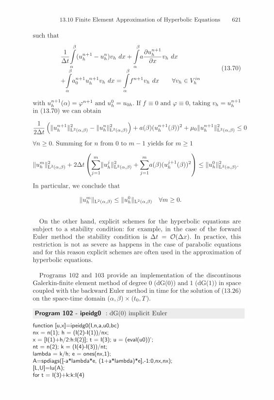
13.10 Finite Element Approximation of Hyperbolic Equations 621
such that
1#t
'
!
(un+1h " un
h)vh dx +
'
!
a.un+1
h
.xvh dx
+
'
!
an+10 un+1
h vh dx =
'
!
fn+1vh dx #vh ! V inh
(13.70)
with un+1h (") = 1n+1 and u0
h = u0h. If f ? 0 and 1 ? 0, taking vh = un+1h
in (13.70) we can obtain
12#t
K+un+1
h +2L2(!,') " +unh+2L2(!,')
L+ a(#)(un+1
h (#))2 + µ0+un+1h +2L2(!,') & 0
#n ) 0. Summing for n from 0 to m" 1 yields for m ) 1
+umh +2L2(!,') + 2#t
G
Hm(
j=1
+ujh+
2L2(!,') +
m(
j=1
a(#)(uj+1h (#))2
I
J & +u0h+2L2(!,').
In particular, we conclude that
+umh +L2(!,') & +u0
h+L2(!,') #m ) 0.
On the other hand, explicit schemes for the hyperbolic equations aresubject to a stability condition: for example, in the case of the forwardEuler method the stability condition is #t = O(#x). In practice, thisrestriction is not as severe as happens in the case of parabolic equationsand for this reason explicit schemes are often used in the approximation ofhyperbolic equations.
Programs 102 and 103 provide an implementation of the discontinousGalerkin-finite element method of degree 0 (dG(0)) and 1 (dG(1)) in spacecoupled with the backward Euler method in time for the solution of (13.26)on the space-time domain (",#)% (t0, T ).
Program 102 - ipeidg0 : dG(0) implicit Euler
function [u,x]=ipeidg0(I,n,a,u0,bc)nx = n(1); h = (I(2)-I(1))/nx;x = [I(1)+h/2:h:I(2)]; t = I(3); u = (eval(u0))’;nt = n(2); k = (I(4)-I(3))/nt;lambda = k/h; e = ones(nx,1);A=spdiags([-a*lambda*e, (1+a*lambda)*e],-1:0,nx,nx);[L,U]=lu(A);for t = I(3)+k:k:I(4)

622 13. Parabolic and Hyperbolic Initial Boundary Value Problems
f = u;if a > 0
f(1) = a*bc(1)+f(1);elseif a <= 0
f(nx) = a*bc(2)+f(nx);endy = L \ f; u = U \ y;
end
Program 103 - ipeidg1 : dG(1) implicit Euler
function [u,x]=ipeidg1(I,n,a,u0,bc)nx = n(1); h = (I(2)-I(1))/nx;x = [I(1):h:I(2)]; t = I(3); um = (eval(u0))’;u = []; xx=[];for i = 1:nx+1
u = [u, um(i), um(i)]; xx = [xx, x(i), x(i)];endu = u’; nt = n(2); k = (I(4)-I(3))/nt;lambda = k/h; e = ones(2*nx+2,1);B = spdiags([1/6*e,1/3*e,1/6*e],-1:1,2*nx+2,2*nx+2);dd = 1/3+0.5*a*lambda; du = 1/6+0.5*a*lambda;dl = 1/6-0.5*a*lambda; A=sparse([]);A(1,1) = dd; A(1,2) = du; A(2,1) = dl; A(2,2) = dd;for i=3:2:2*nx+2
A(i,i-1) =-a*lambda;A(i,i) = dd; A(i,i+1) = du;A(i+1,i) = dl; A(i+1,i+1) = A(i,i);
end[L,U]=lu(A);for t = I(3)+k:k:I(4)
f = B*u;if a > 0
f(1) = a*bc(1)+f(1);elseif a <= 0
f(nx) = a*bc(2)+f(nx);endy = L \ f;u = U \ y;
endx = xx;

13.11 Applications 623
13.11 Applications
13.11.1 Heat Conduction in a BarConsider a homogeneous bar of unit length with thermal conductivity 3,which is connected at the endpoints to an external thermal source at a fixedtemperature, say u = 0. Let u0(x) be the temperature distribution alongthe bar at time t = 0 and f = f(x, t) be a given heat production term.Then, the initial-boundary value problem (13.1)-(13.4) provides a model ofthe time evolution of the temperature u = u(x, t) throughout the bar.In the following, we study the case where f ? 0 and the temperature ofthe bar is suddenly raised at the points around 1/2. A rough mathematicalmodel for this situation is provided, for instance, by taking u0 = K ina certain subinterval [a, b] 7 [0, 1] and equal to 0 outside, where K is agiven positive constant. The initial condition is therefore a discontinuousfunction.
We have used the !-method with ! = 0.5 (Crank-Nicolson method, CN)and ! = 1 (Backward Euler method, BE). Program 100 has been runwith h = 1/20, #t = 1/40 and the obtained solutions at time t = 2 areshown in Figure 13.10. The results show that the CN method su!ers a clearinstability due to the low smoothness of the initial datum (about this point,see also [QV94], Chapter 11). On the contrary, the BE method provides astable solution which decays correctly to zero as t grows since the sourceterm f is null.
0
0.5
1
0
0.5
1
1.5
2
!0.2
0
0.2
0.4
0.6
0.8
00.2
0.40.6
0.81
0
0.5
1
1.5
2
0
0.1
0.2
0.3
0.4
0.5
0.6
0.7
0.8
0.9
1
FIGURE 13.10. Solutions for a parabolic problem with discontinuous initial da-tum: CN method (left) and BE method (right)
13.11.2 A Hyperbolic Model for Blood Flow Interaction withArterial Walls
Let us consider again the problem of the fluid-structure interaction in acylindrical artery considered in Section 11.11.2, where the simple indepen-dent rings model (11.88) was adopted.

624 13. Parabolic and Hyperbolic Initial Boundary Value Problems
If the axial action due to the tension between the di!erent rings isno longer neglected, denoting by z the longitudinal coordinate, equation(11.88) modifies into
)wH.2-
.t2" (z
.2-
.z2 +HE
R20- = P " P0, t > 0, 0 < z < L (13.71)
where (z is the radial component of the axial stress and L is the length ofthe cylindrical arterial district which is considered. In particular, neglectingthe third term on the left hand side and letting '2 = (z/()wH), f =(P " P0)/()wH), we recover the wave equation (13.33).
We have performed two sets of numerical experiments using the Leap-Frog (LF) and Newmark (NW) methods. In the first example the space-time domain of integration is the cylinder (0, 1) % (0, 1) and the sourceterm is f = (1 + &2'2)e"t sin(&x) in such a way that the exact solution isu(x, t) = e"t sin(&x). Table 13.3 shows the estimated orders of convergenceof the two methods, denoted by pLF and pNW respectively.
To compute these quantities we have first solved the wave equation onfour grids with sizes #x = #t = 1/(2k · 10), k = 0, . . . , 3. Let u(k)
h denotethe numerical solution corresponding to the space-time grid at the k-threfining level. Moreover, for j = 1, . . . , 10, let t(0)j = j/10 be the timediscretization nodes of the grid at the coarsest level k = 0. Then, for eachlevel k, the maximum nodal errors ekj on the k-th spatial grid have beenevaluated at each time t(0)j in such a way that the convergence order p(k)
jcan be estimated as
p(k)j =
log(e0j/e
kj )
log(2k), k = 1, 2, 3.
The results clearly show second-order convergence for both the methods,as theoretically expected.
In the second example we have taken the following expressions for thecoe"cient and source term: '2 = (z/()wH), with (z = 1 [Kgs"2], f =(x#p · sin(00t))/()wH). The parameters )w, H and the length L of thevessel are as in Section 11.11.2. The space-time computational domain is(0, L)% (0, T ), with T = 1 [s].
The Newmark method has been first used with #x = L/10 and #t =T/100; the corresponding value of '$ is 3.6515, where $ = #t/#x. Since theNewmark method is unconditionally stable, no spurious oscillations arise asis confirmed by Figure 13.11, left. Notice the correct periodical behaviourof the solution with a period corresponding to one heart beat; notice alsothat with the present values of #t and #x the Leap-Frog method cannotbe employed since the CFL condition is not satisfied. To overcome this

13.12 Exercises 625
t(0)j p(1)LF p(2)
LF p(3)LF
0.1 2.0344 2.0215 2.01510.2 2.0223 2.0139 2.00970.3 2.0170 2.0106 2.00740.4 2.0139 2.0087 2.00610.5 2.0117 2.0073 2.00510.6 2.0101 2.0063 2.00440.7 2.0086 2.0054 2.00380.8 2.0073 2.0046 2.00320.9 2.0059 2.0037 2.00261.0 2.0044 2.0028 2.0019
t(0)j p(1)NW p(2)
NW p(3)NW
0.1 1.9549 1.9718 1.98030.2 1.9701 1.9813 1.98690.3 1.9754 1.9846 1.98920.4 1.9791 1.9869 1.99090.5 1.9827 1.9892 1.99240.6 1.9865 1.9916 1.99410.7 1.9910 1.9944 1.99610.8 1.9965 1.9979 1.99850.9 2.0034 2.0022 2.00151.0 2.0125 2.0079 2.0055
TABLE 13.3. Estimated orders of convergence for the Leap-Frog (LF) and New-mark (NW) methods
problem, we have therefore chosen a much smaller time-step #t = T/400,in such a way that '$ 1 0.9129 and the Leap-Frog scheme can be applied.The obtained result is shown in Figure 13.11, right; a similar solution hasbeen computed by using the Newmark method with the same values of thediscretization parameters.
00.01
0.020.03
0.04
00.20.40.60.81!3
!2
!1
0
1
2
3
x 10!4
00.02
0.040.06
00.20.40.60.81!3
!2
!1
0
1
2
3
x 10!4
FIGURE 13.11. Computed solutions using the NM method on a space-time gridwith $t = T/100 and $x = L/10 (left) and the LF scheme on a space-time gridwith the same value of $x but with $t = T/400 (right)
13.12 Exercises1. Apply the .-method (13.9) to the approximate solution of the scalar Cauchy
problem (11.1) and using the analysis of Section 11.3 prove that the localtruncation error is of the order of $t + h2 if . $= 1
2 while it is of the orderof $t2 + h2 if . = 1
2 .
2. Prove that in the case of piecewise linear finite elements, the mass-lumpingprocess described in Section 13.3 is equivalent to computing the integrals

626 13. Parabolic and Hyperbolic Initial Boundary Value Problems
mij =@ 10 (j(i dx by the trapezoidal quadrature formula (9.11). This, in
particular, shows that the diagonal matrix DM is nonsingular.[Hint: first, verify that exact integration yields
mij =h6
)+
,
12
i $= j,
1 i = j.
Then, apply the trapezoidal rule to compute mij recalling that (i(xj) =!ij .]
3. Prove inequality (13.19).[Hint: using the Cauchy-Schwarz and Young inequalities, prove first that
1^
0
(u% v)u dx ! 12
8&u&2L2(0,1) % &v&
2L2(0,1)
9, ) u, v / L2(0, 1).
Then, use (13.18). ]
4. Assume that the bilinear form a(·, ·) in problem (13.12) is continuous andcoercive over the function space V (see (12.54)-(12.55)) with continuity andcoercivity constants M and $, respectively. Then, prove that the stabilityinequalities (13.20) and (13.21) still hold provided that 2 is replaced by $.
5. Show that the methods (13.39), (13.40) and (13.41) can be written in theform (13.42). Then, show that the corresponding expressions of the artificialviscosity K and artificial di"usion flux hdiff
j+1/2 are as in Table (13.1).
6. Determine the CFL condition for the upwind scheme.
7. Show that for the scheme (13.43) one has &un+1&#,2 " &un&#,2 for alln ! 0.[Hint: multiply equation (13.43) by un+1
j , and notice that
(un+1j % un
j )un+1j ! 1
28|un+1
j |2 % |unj |2
9.
Then, sum on j the resulting inequalities, and note that
#a2
!(
j=%!
8un+1j+1 % un+1
j%19un+1j = 0
since this sum is telescopic.]
8. Show how to find the values µ and 2 in Table 13.2 for Lax-Friedrichs andLax-Wendro" methods.
9. Prove (13.67).
10. Prove (13.69) when f = 0.[Hint: take )t > 0, vh = uh(t) in (13.68).]

References
[Aas71] Aasen J. (1971) On the Reduction of a Symmetric Matrix toTridiagonal Form. BIT 11: 233–242.
[ABB+92] Anderson E., Bai Z., Bischof C., Demmel J., Dongarra J., CrozJ. D., Greenbaum A., Hammarling S., McKenney A., Ous-trouchov S., and Sorensen D. (1992) LAPACK User’s Guide,Release 1.0. SIAM, Philadelphia.
[Ada75] Adams D. (1975) Sobolev Spaces. Academic Press, New York.
[ADR92] Arioli M., Du! I., and Ruiz D. (1992) Stopping Criteria forIterative Solvers. SIAM J. Matrix Anal. Appl. 1(13).
[AF83] Alonso M. and Finn E. (1983) Fundamental UniversityPhysics, volume 3. Addison-Wesley, Reading, Massachusetts.
[Arm66] Armijo L. (1966) Minimization of Functions Having Continu-ous Partial Derivatives. Pacific Jour. Math. 16: 1–3.
[Arn73] Arnold V. I. (1973) Ordinary Di!erential Equations. The MITPress, Cambridge, Massachusetts.
[Atk89] Atkinson K. E. (1989) An Introduction to Numerical Analysis.John Wiley, New York.
[Avr76] Avriel M. (1976) Non Linear Programming: Analysis andMethods. Prentice-Hall, Englewood Cli!s, New Jersey.

628 References
[Axe94] Axelsson O. (1994) Iterative Solution Methods. CambridgeUniversity Press, New York.
[Bar89] Barnett S. (1989) Leverrier’s Algorithm: A New Proof andExtensions. Numer. Math. 7: 338–352.
[Bat90] Batterson S. (1990) Convergence of the Shifted QR Algorithmon 3 by 3 Normal Matrices. Numer. Math. 58: 341–352.
[BBC+94] Barrett R., Berry M., Chan T., Demmel J., Donato J., Don-garra J., Eijkhout V., Pozo V., Romine C., and van der VorstH. (1994) Templates for the Solution of Linear Systems: Build-ing Blocks for Iterative Methods. SIAM, Philadelphia.
[BD74] Bjorck A. and Dahlquist G. (1974) Numerical Methods.Prentice-Hall, Englewood Cli!s, N.J.
[BDMS79] Bunch J., Dongarra J., Moler C., and Stewart G. (1979) LIN-PACK User’s Guide. SIAM, Philadelphia.
[Ber82] Bertsekas D. P. (1982) Constrained Optimization and La-grange Multiplier Methods. Academic Press. Inc., San Diego,California.
[Bjo88] Bjorck A. (1988) Least Squares Methods: Handbook of Numer-ical Analysis Vol. 1 Solution of Equations in RN . ElsevierNorth Holland.
[BM92] Bernardi C. and Maday Y. (1992) Approximations Spectralesdes Problemes aux Limites Elliptiques. Springer-Verlag, Paris.
[BMW67] Barth W., Martin R. S., and Wilkinson J. H. (1967) Calcula-tion of the Eigenvalues of a Symmetric Tridiagonal Matrix bythe Method of Bisection. Numer. Math. 9: 386–393.
[BO78] Bender C. M. and Orszag S. A. (1978) Advanced Mathemati-cal Methods for Scientists and Engineers. McGraw-Hill, NewYork.
[Boe80] Boehm W. (1980) Inserting New Knots into B-spline Curves.Computer Aided Design 12: 199–201.
[Bos93] Bossavit A. (1993) Electromagnetisme, en vue de la modelisa-tion. Springer-Verlag, Paris.
[BR81] Bank R. E. and Rose D. J. (1981) Global Approximate NewtonMethods. Numer. Math. 37: 279–295.
[Bra75] Bradley G. (1975) A Primer of Linear Algebra. Prentice-Hall,Englewood Cli!s, New York.

References 629
[Bre73] Brent R. (1973) Algorithms for Minimization Without Deriva-tives. Prentice-Hall, Englewood Cli!s, New York.
[Bri74] Brigham E. O. (1974) The Fast Fourier Transform. Prentice-Hall, Englewood Cli!s, New York.
[BS90] Brown P. and Saad Y. (1990) Hybrid Krylov Methods for Non-linear Systems of equations. SIAM J. Sci. and Stat. Comput.11(3): 450–481.
[BSG96] B. Smith P. B. and Gropp P. (1996) Domain Decomposition,Parallel Multilevel Methods for Elliptic Partial Di!erentialEquations. Univ. Cambridge Press, Cambridge.
[But64] Butcher J. C. (1964) Implicit Runge-Kutta Processes. Math.Comp. 18: 233–244.
[But66] Butcher J. C. (1966) On the Convergence of Numerical So-lutions to Ordinary Di!erential Equations. Math. Comp. 20:1–10.
[But87] Butcher J. (1987) The Numerical Analysis of Ordinary Di!er-ential Equations: Runge-Kutta and General Linear Methods.Wiley, Chichester.
[CCP70] Cannon M., Cullum C., and Polak E. (1970) Theory and Op-timal Control and Mathematical Programming. McGraw-Hill,New York.
[CFL28] Courant R., Friedrichs K., and Lewy H. (1928) Uber diepartiellen di!erenzengleichungen der mathematischen physik.Math. Ann. 100: 32–74.
[CHQZ88] Canuto C., Hussaini M. Y., Quarteroni A., and Zang T. A.(1988) Spectral Methods in Fluid Dynamics. Springer, NewYork.
[CI95] Chandrasekaren S. and Ipsen I. (1995) On the Sensitivity ofSolution Components in Linear Systems of equations. SIAMJ. Matrix Anal. Appl. 16: 93–112.
[CL91] Ciarlet P. G. and Lions J. L. (1991) Handbook of NumericalAnalysis: Finite Element Methods (Part 1). North-Holland,Amsterdam.
[CM94] Chan T. and Mathew T. (1994) Domain Decomposition Algo-rithms. Acta Numerica pages 61–143.

630 References
[CMSW79] Cline A., Moler C., Stewart G., and Wilkinson J. (1979) AnEstimate for the Condition Number of a Matrix. SIAM J. Sci.and Stat. Comput. 16: 368–375.
[Col66] Collin R. E. (1966) Foundations for Microwave Engineering.McGraw-Hill Book Co., Singapore.
[Com95] Comincioli V. (1995) Analisi Numerica Metodi Modelli Appli-cazioni. McGraw-Hill Libri Italia, Milano.
[Cox72] Cox M. (1972) The Numerical Evaluation of B-splines. Jour-nal of the Inst. of Mathematics and its Applications 10: 134–149.
[Cry73] Cryer C. W. (1973) On the Instability of High OrderBackward-Di!erence Multistep Methods. BIT 13: 153–159.
[CT65] Cooley J. and Tukey J. (1965) An Algorithm for the MachineCalculation of Complex Fourier Series. Math. Comp. 19: 297–301.
[Dah56] Dahlquist G. (1956) Convergence and Stability in the Nu-merical Integration of Ordinary Di!erential Equations. Math.Scand. 4: 33–53.
[Dah63] Dahlquist G. (1963) A Special Stability Problem for LinearMultistep Methods. BIT 3: 27–43.
[Dat95] Datta B. (1995) Numerical Linear Algebra and Applications.Brooks/Cole Publishing, Pacific Grove, CA.
[Dau88] Daubechies I. (1988) Orthonormal bases of compactly sup-ported wavelets. Commun. on Pure and Appl. Math. XLI.
[Dav63] Davis P. (1963) Interpolation and Approximation. BlaisdellPub., New York.
[Day96] Day D. (1996) How the QR algorithm Fails to Converge andHow to Fix It. Technical Report 96-0913J, Sandia NationalLaboratory, Albuquerque.
[dB72] de Boor C. (1972) On Calculating with B-splines. Journal ofApproximation Theory 6: 50–62.
[dB83] de Boor C. (1983) A Practical Guide to Splines. In AppliedMathematical Sciences. (27), Springer-Verlag, New York.
[dB90] de Boor C. (1990) SPLINE TOOLBOX for use with MAT-LAB. The Math Works, Inc., South Natick.

References 631
[DD95] Davis T. and Du! I. (1995) A combinedunifrontal/multifrontal method for unsymmetric sparsematrices. Technical Report TR-95-020, Computer andInformation Sciences Department, University of Florida.
[Dek69] Dekker T. (1969) Finding a Zero by means of Successive LinearInterpolation. In Dejon B. and Henrici P. (eds) ConstructiveAspects of the Fundamental Theorem of Algebra, pages 37–51.Wiley, New York.
[Dek71] Dekker T. (1971) A Floating-Point Technique for Extendingthe Available Precision. Numer. Math. 18: 224–242.
[Dem97] Demmel J. (1997) Applied Numerical Linear Algebra. SIAM,Philadelphia.
[DGK84] Dongarra J., Gustavson F., and Karp A. (1984) ImplementingLinear Algebra Algorithms for Dense Matrices on a VectorPipeline Machine. SIAM Review 26(1): 91–112.
[Die87a] Dierckx P. (1987) FITPACK User Guide part 1: Curve FittingRoutines. TW Report, Dept. of Computer Science, KatholiekeUniversiteit, Leuven, Belgium.
[Die87b] Dierckx P. (1987) FITPACK User Guide part 2: SurfaceFitting Routines. TW Report, Dept. of Computer Science,Katholieke Universiteit, Leuven, Belgium.
[Die93] Dierckx P. (1993) Curve and Surface Fitting with Splines.Claredon Press, New York.
[DL92] DeVore R. and Lucier J. (1992) Wavelets. Acta Numericapages 1–56.
[DR75] Davis P. and Rabinowitz P. (1975) Methods of Numerical In-tegration. Academic Press, New York.
[DS83] Dennis J. and Schnabel R. (1983) Numerical Methods for Un-constrained Optimization and Nonlinear Equations. Prentice-Hall, Englewood Cli!s, New York.
[Dun85] Dunavant D. (1985) High Degree E"cient Symmetrical Gaus-sian Quadrature Rules for the Triangle. Internat. J. Numer.Meth. Engrg. 21: 1129–1148.
[Dun86] Dunavant D. (1986) E"cient Symmetrical Cubature Rules forComplete Polynomials of High Degree over the Unit Cube.Internat. J. Numer. Meth. Engrg. 23: 397–407.

632 References
[DV84] Dekker K. and Verwer J. (1984) Stability of Runge-KuttaMethods for Sti! Nonlinear Di!erential Equations. North-Holland, Amsterdam.
[dV89] der Vorst H. V. (1989) High Performance Preconditioning.SIAM J. Sci. Stat. Comput. 10: 1174–1185.
[EEHJ96] Eriksson K., Estep D., Hansbo P., and Johnson C. (1996)Computational Di!erential Equations. Cambridge Univ.Press, Cambridge.
[Elm86] Elman H. (1986) A Stability Analisys of Incomplete LU Fac-torization. Math. Comp. 47: 191–218.
[Erd61] Erdos P. (1961) Problems and Results on the Theory of Inter-polation. Acta Math. Acad. Sci. Hungar. 44: 235–244.
[Erh97] Erhel J. (1997) About Newton-Krylov Methods. In Periaux J.and al. (eds) Computational Science for 21st Century, pages53–61. Wiley, New York.
[Fab14] Faber G. (1914) Uber die interpolatorische Darstellungstetiger Funktionem. Jber. Deutsch. Math. Verein. 23: 192–210.
[FF63] Faddeev D. K. and Faddeeva V. N. (1963) ComputationalMethods of Linear Algebra. Freeman, San Francisco and Lon-don.
[Fle75] Fletcher R. (1975) Conjugate gradient methods for indefinitesystems. In Springer-Verlag (ed) Numerical Analysis, pages73–89. New York.
[FM67] Forsythe G. E. and Moler C. B. (1967) Computer Solutionof Linear Algebraic Systems. Prentice-Hall, Englewood Cli!s,New York.
[Fra61] Francis J. G. F. (1961) The QR Transformation: A UnitaryAnalogue to the LR Transformation. Parts I and II. Comp. J.pages 265–272,332–334.
[FRL55] F. Richtmyer E. K. and Lauritsen T. (1955) Introduction toModern Physics. McGraw-Hill, New York.
[Gas83] Gastinel N. (1983) Linear Numerical Analysis. Kershaw Pub-lishing, London.

References 633
[Gau94] Gautschi W. (1994) Algorithm 726: ORTHPOL - A Package ofRoutines for Generating Orthogonal Polynomials and Gauss-type Quadrature Rules. ACM Trans. Math. Software 20: 21–62.
[Gau96] Gautschi W. (1996) Orthogonal Polynomials: Applicationsand Computation. Acta Numerica pages 45–119.
[Gau97] Gautschi W. (1997) Numerical Analysis. An Introduction.Birkhauser, Berlin.
[Geo73] George A. (1973) Nested Dissection of a Regular Finite Ele-ment Mesh. SIAM J. Num. Anal. 10: 345–363.
[Giv54] Givens W. (1954) Numerical Computation of the Character-istic Values of a Real Symmetric Matrix. Oak Ridge NationalLaboratory ORNL-1574.
[GL81] George A. and Liu J. (1981) Computer Solution of LargeSparse Positive Definite Systems. Prentice-Hall, EnglewoodCli!s, New York.
[GL89] Golub G. and Loan C. V. (1989) Matrix Computations. TheJohn Hopkins Univ. Press, Baltimore and London.
[GM83] Golub G. and Meurant G. (1983) Resolution Numerique desGrands Systemes Lineaires. Eyrolles, Paris.
[GMW81] Gill P., Murray W., and Wright M. (1981) Practical Optimiza-tion. Academic Press, London.
[God66] Godeman R. (1966) Algebra. Kershaw, London.
[Gol91] Goldberg D. (1991) What Every Computer Scientist ShouldKnow about Floating-point Arithmetic. ACM ComputingSurveys 23(1): 5–48.
[GP67] Goldstein A. A. and Price J. B. (1967) An E!ective Algorithmfor Minimization. Numer. Math 10: 184–189.
[GR96] Godlewski E. and Raviart P. (1996) Numerical Approximationof Hyperbolic System of Conservation Laws, volume 118 ofApplied Mathematical Sciences. Springer-Verlag, New York.
[Hac94] Hackbush W. (1994) Iterative Solution of Large Sparse Sys-tems of Equations. Springer-Verlag, New York.
[Hah67] Hahn W. (1967) Stability of Motion. Springer-Verlag, Berlin.

634 References
[Hal58] Halmos P. (1958) Finite-Dimensional Vector Spaces. Van Nos-trand, Princeton, New York.
[Hen62] Henrici P. (1962) Discrete Variable Methods in Ordinary Dif-ferential Equations. Wiley, New York.
[Hen74] Henrici P. (1974) Applied and Computational Complex Anal-ysis, volume 1. Wiley, New York.
[HGR96] H-G. Roos M. Stynes L. T. (1996) Numerical Methods forSingularly Perturbed Di!erential Equations. Springer-Verlag,Berlin Heidelberg.
[Hig88] Higham N. (1988) The Accuracy of Solutions to TriangularSystems. University of Manchester, Dep. of Mathematics 158:91–112.
[Hig89] Higham N. (1989) The Accuracy of Solutions to TriangularSystems. SIAM J. Numer. Anal. 26(5): 1252–1265.
[Hig96] Higham N. (1996) Accuracy and Stability of Numerical Algo-rithms. SIAM Publications, Philadelphia, PA.
[Hil87] Hildebrand F. (1987) Introduction to Numerical Analysis.McGraw-Hill, New York.
[Hou75] Householder A. (1975) The Theory of Matrices in NumericalAnalysis. Dover Publications, New York.
[HP94] Hennessy J. and Patterson D. (1994) Computer Organiza-tion and Design - The Hardware/Software Interface. MorganKaufmann, San Mateo.
[HW76] Hammarling S. and Wilkinson J. (1976) The Practical Be-haviour of Linear Iterative Methods with Particular Referenceto S.O.R. Technical Report Report NAC 69, National Physi-cal Laboratory, Teddington, UK.
[IK66] Isaacson E. and Keller H. (1966) Analysis of Numerical Meth-ods. Wiley, New York.
[Inm94] Inman D. (1994) Engineering Vibration. Prentice-Hall, Engle-wood Cli!s, NJ.
[Iro70] Irons B. (1970) A Frontal Solution Program for Finite ElementAnalysis. Int. J. for Numer. Meth. in Engng. 2: 5–32.
[Jac26] Jacobi C. (1826) Uber Gau# neue Methode, die Werthe derIntegrale naherungsweise zu finden. J. Reine Angew. Math.30: 127–156.

References 635
[Jer96] Jerome J. J. (1996) Analysis of Charge Transport. A Math-ematical Study of Semiconductor Devices. Springer, BerlinHeidelberg.
[Jia95] Jia Z. (1995) The Convergence of Generalized Lanczos Meth-ods for Large Unsymmetric Eigenproblems. SIAM J. MatrixAnal. Applic. 16: 543–562.
[JM92] Jennings A. and McKeown J. (1992) Matrix Computation.Wiley, Chichester.
[Joh90] Johnson C. (1990) Numerical Solution of Partial Di!erentialEquations by the Finite Element Method. Cambridge Univ.Press.
[JW77] Jankowski M. and Wozniakowski M. (1977) Iterative Refine-ment Implies Numerical Stability. BIT 17: 303–311.
[Kah66] Kahan W. (1966) Numerical Linear Algebra. Canadian Math.Bull. 9: 757–801.
[Kan66] Kaniel S. (1966) Estimates for Some Computational Tech-niques in Linear Algebra. Math. Comp. 20: 369–378.
[Kea86] Keast P. (1986) Moderate-Degree Tetrahedral QuadratureFormulas. Comp. Meth. Appl. Mech. Engrg. 55: 339–348.
[Kel99] Kelley C. (1999) Iterative Methods for Optimization, vol-ume 18 of Frontiers in Applied Mathematics. SIAM, Philadel-phia.
[KT51] Kuhn H. and Tucker A. (1951) Nonlinear Programming. InSecond Berkeley Symposium on Mathematical Statistics andProbability, pages 481–492. Univ. of California Press, Berkeleyand Los Angeles.
[Lam91] Lambert J. (1991) Numerical Methods for Ordinary Di!eren-tial Systems. John Wiley and Sons, Chichester.
[Lan50] Lanczos C. (1950) An Iteration Method for the Solution of theEigenvalue Problem of Linear Di!erential and Integral Oper-ator. J. Res. Nat. Bur. Stand. 45: 255–282.
[Lax65] Lax P. (1965) Numerical Solution of Partial Di!erential Equa-tions. Amer. Math. Monthly 72(2): 74–84.
[Lel92] Lele S. (1992) Compact Finite Di!erence Schemes withSpectral-like Resolution. Journ. of Comp. Physics 103(1): 16–42.

636 References
[Lem89] Lemarechal C. (1989) Nondi!erentiable Optimization. InNemhauser G., Kan A. R., and Todd M. (eds) HandbooksOper. Res. Management Sci., volume 1. Optimization, pages529–572. North-Holland, Amsterdam.
[LH74] Lawson C. and Hanson R. (1974) Solving Least Squares Prob-lems. Prentice-Hall, Englewood Cli!s, New York.
[LM68] Lions J. L. and Magenes E. (1968) Problemes aux limites non-homogenes et applications. Dunod, Paris.
[LS96] Lehoucq R. and Sorensen D. (1996) Deflation Techniques foran Implicitly Restarted Iteration. SIAM J. Matrix Anal. Ap-plic. 17(4): 789–821.
[Lue73] Luenberger D. (1973) Introduction to Linear and Non LinearProgramming. Addison-Wesley, Reading, Massachusetts.
[Man69] Mangasarian O. (1969) Non Linear Programming. Prentice-Hall, Englewood Cli!s, New Jersey.
[Man80] Manteu!el T. (1980) An Incomplete Factorization Techniquefor Positive Definite Linear Systems. Math. Comp. 150(34):473–497.
[Mar86] Markowich P. (1986) The Stationary Semiconductor DeviceEquations. Springer-Verlag, Wien and New York.
[McK62] McKeeman W. (1962) Crout with Equilibration and Iteration.Comm. ACM 5: 553–555.
[MdV77] Meijerink J. and der Vorst H. V. (1977) An Iterative SolutionMethod for Linear Systems of Which the Coe"cient Matrix isa Symmetric M-matrix. Math. Comp. 137(31): 148–162.
[MM71] Maxfield J. and Maxfield M. (1971) Abstract Algebra and So-lution by Radicals. Saunders, Philadelphia.
[MMG87] Martinet R., Morlet J., and Grossmann A. (1987) Analysis ofsound patterns through wavelet transforms. Int. J. of PatternRecogn. and Artificial Intellig. 1(2): 273–302.
[MNS74] Makela M., Nevanlinna O., and Sipila A. (1974) On the Con-cept of Convergence, Consistency and Stability in Connectionwith Some Numerical Methods. Numer. Math. 22: 261–274.
[Mor84] Morozov V. (1984) Methods for Solving Incorrectly PosedProblems. Springer-Verlag, New York.

References 637
[Mul56] Muller D. (1956) A Method for Solving Algebraic Equationsusing an Automatic Computer. Math. Tables Aids Comput.10: 208–215.
[ NAG95] NAG (1995) NAG Fortran Library Manual - Mark 17. NAGLtd., Oxford.
[Nat65] Natanson I. (1965) Constructive Function Theory, volume III.Ungar, New York.
[NM65] Nelder J. and Mead R. (1965) A simplex method for functionminimization. The Computer Journal 7: 308–313.
[Nob69] Noble B. (1969) Applied Linear Algebra. Prentice-Hall, Engle-wood Cli!s, New York.
[OR70] Ortega J. and Rheinboldt W. (1970) Iterative Solution of Non-linear Equations in Several Variables. Academic Press, NewYork and London.
[Pap62] Papoulis A. (1962) The Fourier Integral and its Application.McGraw-Hill, New York.
[Pap87] Papoulis A. (1987) Probability, Random Variables, andStochastic Processes. McGraw-Hill, New York.
[Par80] Parlett B. (1980) The Symmetric Eigenvalue Problem.Prentice-Hall, Englewood Cli!s, NJ.
[PdKUK83] Piessens R., deDoncker Kapenga E., Uberhuber C. W., andKahaner D. K. (1983) QUADPACK: A Subroutine Packagefor Automatic Integration. Springer-Verlag, Berlin and Hei-delberg.
[PJ55] Peaceman D. and Jr. H. R. (1955) The numerical solution ofparabolic and elliptic di!erential equations. J. Soc. Ind. Appl.Math. 3: 28–41.
[Pou96] Poularikas A. (1996) The Transforms and Applications Hand-book. CRC Press, Inc., Boca Raton, Florida.
[PR70] Parlett B. and Reid J. (1970) On the Solution of a System ofLinear Equations Whose Matrix is Symmetric but not Defi-nite. BIT 10: 386–397.
[PS91] Pagani C. and Salsa S. (1991) Analisi Matematica, volume II.Masson, Milano.

638 References
[PW79] Peters G. and Wilkinson J. (1979) Inverse iteration, ill-conditioned equations, and newton’s method. SIAM Review21: 339–360.
[QV94] Quarteroni A. and Valli A. (1994) Numerical Approximationof Partial Di!erential Equations. Springer, Berlin and Heidel-berg.
[QV99] Quarteroni A. and Valli A. (1999) Domain DecompositionMethods for Partial Di!erential Equations. Oxford SciencePublications, New York.
[Ral65] Ralston A. (1965) A First Course in Numerical Analysis.McGraw-Hill, New York.
[Red86] Reddy B. D. (1986) Applied Functional Analysis and Varia-tional Methods in Engineering. McGraw-Hill, New York.
[Ric81] Rice J. (1981) Matrix Computations and Mathematical Soft-ware. McGraw-Hill, New York.
[Riv74] Rivlin T. (1974) The Chebyshev Polynomials. John Wiley andSons, New York.
[RM67] Richtmyer R. and Morton K. (1967) Di!erence Methods forInitial Value Problems. Wiley, New York.
[RR78] Ralston A. and Rabinowitz P. (1978) A First Course in Nu-merical Analysis. McGraw-Hill, New York.
[Rud83] Rudin W. (1983) Real and Complex Analysis. Tata McGraw-Hill, New Delhi.
[Rut58] Rutishauser H. (1958) Solution of Eigenvalue Problems withthe LR Transformation. Nat. Bur. Stand. Appl. Math. Ser.49: 47–81.
[Saa90] Saad Y. (1990) Sparskit: A basic tool kit for sparse matrixcomputations. Technical Report 90-20, Research Institute forAdvanced Computer Science, NASA Ames Research Center,Mo!et Field, CA.
[Saa92] Saad Y. (1992) Numerical Methods for Large Eigenvalue Prob-lems. Halstead Press, New York.
[Saa96] Saad Y. (1996) Iterative Methods for Sparse Linear Systems.PWS Publishing Company, Boston.
[Sch67] Schoenberg I. (1967) On Spline functions. In Shisha O. (ed)Inequalities, pages 255–291. Academic Press, New York.
References 639
[Sch81] Schumaker L. (1981) Splines Functions: Basic Theory. Wiley,New York.
[Sel84] Selberherr S. (1984) Analysis and Simulation of Semiconduc-tor Devices. Springer-Verlag, Wien and New York.
[SG69] Scharfetter D. and Gummel H. (1969) Large-signal analysis ofa silicon Read diode oscillator. IEEE Trans. on Electr. Dev.16: 64–77.
[Ske79] Skeel R. (1979) Scaling for Numerical Stability in GaussianElimination. J. Assoc. Comput. Mach. 26: 494–526.
[Ske80] Skeel R. (1980) Iterative Refinement Implies Numerical Sta-bility for Gaussian Elimination. Math. Comp. 35: 817–832.
[SL89] Su B. and Liu D. (1989) Computational Geometry: Curve andSurface Modeling. Academic Press, New York.
[Sla63] Slater J. (1963) Introduction to Chemical Physics. McGraw-Hill Book Co.
[Smi85] Smith G. (1985) Numerical Solution of Partial Di!erentialEquations: Finite Di!erence Methods. Oxford UniversityPress, Oxford.
[Son89] Sonneveld P. (1989) Cgs, a fast lanczos-type solver for non-symmetric linear systems. SIAM Journal on Scientific andStatistical Computing 10(1): 36–52.
[SR97] Shampine L. F. and Reichelt M. W. (1997) The MATLABODE Suite. SIAM J. Sci. Comput. 18: 1–22.
[SS90] Stewart G. and Sun J. (1990) Matrix Perturbation Theory.Academic Press, New York.
[SS98] Schwab C. and Schotzau D. (1998) Mixed hp-FEM onAnisotropic Meshes. Mat. Models Methods Appl. Sci. 8(5):787–820.
[Ste71] Stetter H. (1971) Stability of discretization on infinite inter-vals. In Morris J. (ed) Conf. on Applications of NumericalAnalysis, pages 207–222. Springer-Verlag, Berlin.
[Ste73] Stewart G. (1973) Introduction to Matrix Computations. Aca-demic Press, New York.
[Str69] Strassen V. (1969) Gaussian Elimination is Not Optimal. Nu-mer. Math. 13: 727–764.

640 References
[Str80] Strang G. (1980) Linear Algebra and Its Applications. Aca-demic Press, New York.
[Str89] Strikwerda J. (1989) Finite Di!erence Schemes and PartialDi!erential Equations. Wadsworth and Brooks/Cole, PacificGrove.
[Sze67] Szego G. (1967) Orthogonal Polynomials. AMS, Providence,R.I.
[Tit37] Titchmarsh E. (1937) Introduction to the Theory of FourierIntegrals. Oxford.
[Var62] Varga R. (1962) Matrix Iterative Analysis. Prentice-Hall, En-glewood Cli!s, New York.
[vdV92] van der Vorst H. (1992) Bi-cgstab: a fast and smoothly con-verging variant of bi-cg for the solution of non-symmetric lin-ear systems. SIAM Jour. on Sci. and Stat. Comp. 12: 631–644.
[Ver96] Verfurth R. (1996) A Review of a Posteriori Error Estimationand Adaptive Mesh Refinement Techniques. Wiley, Teubner,Germany.
[Wac66] Wachspress E. (1966) Iterative Solutions of Elliptic Systems.Prentice-Hall, Englewood Cli!s, New York.
[Wal75] Walsh G. (1975) Methods of Optimization. Wiley.
[Wal91] Walker J. (1991) Fast Fourier Transforms. CRC Press, BocaRaton.
[Wen66] Wendro! B. (1966) Theoretical Numerical Analysis. AcademicPress, New York.
[Wid67] Widlund O. (1967) A Note on Unconditionally Stable LinearMultistep Methods. BIT 7: 65–70.
[Wil62] Wilkinson J. (1962) Note on the Quadratic Convergence ofthe Cyclic Jacobi Process. Numer. Math. 6: 296–300.
[Wil63] Wilkinson J. (1963) Rounding Errors in Algebraic Processes.Prentice-Hall, Englewood Cli!s, New York.
[Wil65] Wilkinson J. (1965) The Algebraic Eigenvalue Problem.Clarendon Press, Oxford.
[Wil68] Wilkinson J. (1968) A priori Error Analysis of Algebraic Pro-cesses. In Intern. Congress Math., volume 19, pages 629–639.Izdat. Mir, Moscow.
References 641
[Wol69] Wolfe P. (1969) Convergence Conditions for Ascent Methods.SIAM Review 11: 226–235.
[Wol71] Wolfe P. (1971) Convergence Conditions for Ascent Methods.II: Some Corrections. SIAM Review 13: 185–188.
[Wol78] Wolfe M. (1978) Numerical Methods for Unconstrained Opti-mization. Van Nostrand Reinhold Company, New York.
[You71] Young D. (1971) Iterative Solution of Large Linear Systems.Academic Press, New York.
[Zie77] Zienkiewicz O. C. (1977) The Finite Element Method (ThirdEdition). McGraw Hill, London.
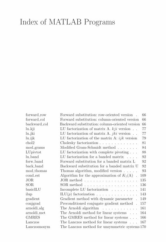
Index of MATLAB Programs
forward row Forward substitution: row-oriented version . 66forward col Forward substitution: column-oriented version 66backward col Backward substitution: column-oriented version 66lu kji LU factorization of matrix A. kji version . . 77lu jki LU factorization of matrix A. jki version . . 77lu ijk LU factorization of the matrix A: ijk version 79chol2 Cholesky factorization . . . . . . . . . . . . . 81mod grams Modified Gram-Schmidt method . . . . . . . 84LUpivtot LU factorization with complete pivoting . . . 88lu band LU factorization for a banded matrix . . . . 92forw band Forward substitution for a banded matrix L 92back band Backward substitution for a banded matrix U 92mod thomas Thomas algorithm, modified version . . . . . 93cond est Algorithm for the approximation of K1(A) . 109JOR JOR method . . . . . . . . . . . . . . . . . . 135SOR SOR method . . . . . . . . . . . . . . . . . . 136basicILU Incomplete LU factorization . . . . . . . . . 141ilup ILU(p) factorization . . . . . . . . . . . . . . 143gradient Gradient method with dynamic parameter . 149conjgrad Preconditioned conjugate gradient method . 157arnoldi alg The Arnoldi algorithm . . . . . . . . . . . . 161arnoldi met The Arnoldi method for linear systems . . . 164GMRES The GMRES method for linear systems . . . 166Lanczos The Lanczos method for linear systems . . . 167Lanczosnosym The Lanczos method for unsymmetric systems170

644 Index of MATLAB Programs
powerm Power method . . . . . . . . . . . . . . . . . 197invpower Inverse power method . . . . . . . . . . . . . 198basicqr Basic QR iteration . . . . . . . . . . . . . . . 203houshess Hessenberg-Householder method . . . . . . . 208hessqr Hessenberg-QR method . . . . . . . . . . . . 210givensqr QR factorization with Givens rotations . . . 211vhouse Construction of the Householder vector . . . 213givcos Computation of Givens cosine and sine . . . 214garow Product G(i, k, !)TM . . . . . . . . . . . . . 214gacol Product MG(i, k, !) . . . . . . . . . . . . . . 214qrshift QR iteration with single shift . . . . . . . . . 217qr2shift QR iteration with double shift . . . . . . . . 220psinorm Evaluation of )(A) . . . . . . . . . . . . . . 229symschur Evaluation of c and s . . . . . . . . . . . . . 229cycjacobi Cyclic Jacobi method for symmetric matrices 229sturm Sturm sequence evaluation . . . . . . . . . . 232givsturm Givens method using the Sturm sequence . . 232chcksign Sign changes in the Sturm sequence . . . . . 232bound Calculation of the interval J = [",#] . . . . 232eiglancz Extremal eigenvalues of a symmetric matrix 234bisect Bisection method . . . . . . . . . . . . . . . 250chord The chord method . . . . . . . . . . . . . . . 254secant The secant method . . . . . . . . . . . . . . 255regfalsi The Regula Falsi method . . . . . . . . . . . 255newton Newton’s method . . . . . . . . . . . . . . . 255fixpoint Fixed-point method . . . . . . . . . . . . . . 260horner Synthetic division algorithm . . . . . . . . . 263newthorn Newton-Horner method with refinement . . . 266mulldefl Muller’s method with refinement . . . . . . . 269aitken Aitken’s extrapolation . . . . . . . . . . . . . 274adptnewt Adaptive Newton’s method . . . . . . . . . . 276newtonxsys Newton’s method for nonlinear systems . . . 285broyden Broyden’s method for nonlinear systems . . . 290fixposys Fixed-point method for nonlinear systems . . 293hookejeeves The method of Hooke and Jeeves (HJ) . . . 296explore Exploration step in the HJ method . . . . . 297backtrackr Backtraking for line search . . . . . . . . . . 303lagrpen Penalty method . . . . . . . . . . . . . . . . 316lagrmult Method of Lagrange multipliers . . . . . . . 319interpol Lagrange polynomial using Newton’s formula 334dividif Newton divided di!erences . . . . . . . . . . 336hermpol Osculating polynomial . . . . . . . . . . . . . 342par spline Parametric splines . . . . . . . . . . . . . . . 359bernstein Bernstein polynomials . . . . . . . . . . . . . 361bezier Bezier curves . . . . . . . . . . . . . . . . . . 361

Index of MATLAB Programs 645
midpntc Midpoint composite formula . . . . . . . . . 375trapezc Composite trapezoidal formula . . . . . . . . 376simpsonc Composite Cavalieri-Simpson formula . . . . 377newtcot Closed Newton-Cotes formulae . . . . . . . . 383trapmodc Composite corrected trapezoidal formula . . 387romberg Romberg integration . . . . . . . . . . . . . . 391simpadpt Adaptive Cavalieri-Simpson formula . . . . . 397redmidpt Midpoint reduction formula . . . . . . . . . . 404redtrap Trapezoidal reduction formula . . . . . . . . 404midptr2d Midpoint rule on a triangle . . . . . . . . . . 406traptr2d Trapezoidal rule on a triangle . . . . . . . . 406coeflege Coe"cients of Legendre polynomials . . . . . 430coeflagu Coe"cients of Laguerre polynomials . . . . . 430coefherm Coe"cients of Hermite polynomials . . . . . 430zplege Coe"cients of Gauss-Legendre formulae . . . 430zplagu Coe"cients of Gauss-Laguerre formulae . . . 430zpherm Coe"cients of Gauss-Hermite formulae . . . 430dft Discrete Fourier transform . . . . . . . . . . 439idft Inverse discrete Fourier transform . . . . . . 439!trec FFT algorithm in the recursive version . . . 441compdi! Compact di!erence schemes . . . . . . . . . 446multistep Linear multistep methods . . . . . . . . . . . 490predcor Predictor-corrector scheme . . . . . . . . . . 507ellfem Linear FE for two-point BVPs . . . . . . . . 557femmatr Construction of the sti!ness matrix . . . . . 557H1error Computation of the H1-norm of the error . 558artvisc Artificial viscosity . . . . . . . . . . . . . . . 570sgvisc Optimal artificial viscosity . . . . . . . . . . 570bern Evaluation of the Bernoulli function . . . . . 571thetameth !-method for the heat equation . . . . . . . . 592pardg1cg1 dG(1)cG(1) method for the heat equation . . 596ipeidg0 dG(0) implicit Euler . . . . . . . . . . . . . . 621ipeidg1 dG(1) implicit Euler . . . . . . . . . . . . . . 622
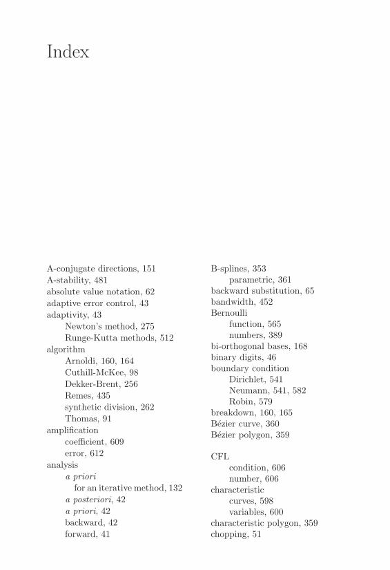
Index
A-conjugate directions, 151A-stability, 481absolute value notation, 62adaptive error control, 43adaptivity, 43
Newton’s method, 275Runge-Kutta methods, 512
algorithmArnoldi, 160, 164Cuthill-McKee, 98Dekker-Brent, 256Remes, 435synthetic division, 262Thomas, 91
amplificationcoe"cient, 609error, 612
analysisa priori
for an iterative method, 132a posteriori, 42a priori, 42backward, 42forward, 41
B-splines, 353parametric, 361
backward substitution, 65bandwidth, 452Bernoulli
function, 565numbers, 389
bi-orthogonal bases, 168binary digits, 46boundary condition
Dirichlet, 541Neumann, 541, 582Robin, 579
breakdown, 160, 165Bezier curve, 360Bezier polygon, 359
CFLcondition, 606number, 606
characteristiccurves, 598variables, 600
characteristic polygon, 359chopping, 51

648 Index
cofactor, 9condition number, 34
asymptotic, 38interpolation, 332of a matrix, 36, 58of a nonlinear equation, 246of an eigenvalue, 189of an eigenvector, 190Skeel, 111spectral, 59
consistency, 37, 124, 474, 493, 510convex function, 295, 321
strongly, 312convex hull, 98critical point, 295
Dahlquistfirst barrier, 499second barrier, 500
decompositionreal Schur, 201, 210, 211
generalized, 225Schur, 14singular value, 16
computation of the, 222spectral, 15
deflation, 207, 216, 263degree
of exactness, 380of a vector, 160of exactness, 372, 380, 405,
420of freedom, 552
determinant of a matrix, 8discrete
truncation of Fourier series,417
Chebyshev transform, 426Fourier transform, 438Laplace transform, 458Legendre transform, 428maximum principle, 567, 611scalar product, 425
dispersion, 448, 612dissipation, 612
distribution, 547derivative of a, 547
divided di!erence, 267, 334domain of dependence, 600
numerical, 606
eigenfunctions, 589eigenvalue, 12
algebraic multiplicity of an,13
geometric multiplicity of an,13
eigenvector, 12elliptic
operator, 602equation
characteristic, 12di!erence, 482, 483, 499heat, 581, 592
errorabsolute, 40cancellation, 39global truncation, 474interpolation, 329local truncation, 474, 605quadrature, 372rounding, 45
estimatea posteriori, 64, 195, 196, 381,
392, 395a priori, 60, 381, 392, 395
exponential fitting, 565
factorasymptotic convergence, 125convergence, 125, 245, 259growth, 104
factorizationblock LU, 94Cholesky, 80compact forms, 78Crout, 78Doolittle, 78incomplete, 140LDMT , 79

Index 649
LU, 68QR, 82, 209
fill-in, 98, 141level, 141
finite di!erences, 118, 177, 237,533
backward, 443centered, 443, 444compact, 444forward, 442
finite elements, 118, 347discontinuous, 594, 619
fixed-point iterations, 257flop, 53FOM, 163, 164form
divided di!erence, 334Lagrange, 329
formulaArmijo’s, 304Goldstein’s, 304Sherman-Morrison, 95
forward substitution, 65Fourier coe"cients, 436
discrete, 437function
gamma, 528Green’s, 532Haar, 460stability, 516weight, 415
Galerkinfinite element method, 364,
550stabilized, 568
generalized method, 559method, 544pseudo-spectral approximation,
591Gauss elimination
method, 68multipliers in the, 69
GAXPY, 77generalized inverse, 17
Gershgorin circles, 184Gibbs phenomenon, 439gradient, 294graph, 97
oriented, 97, 186Gronwall lemma, 471, 476
hyperbolicoperator, 602
hypernorms, 63
ILU, 140inequality
Cauchy-Schwarz, 340, 568Holder, 19Kantorovich, 305Poincare, 536, 569triangular, 569Young’s, 544
integrationadaptive, 391automatic, 391multidimensional, 402non adaptive, 391
interpolationHermite, 341in two dimensions, 343osculatory, 342piecewise, 338Taylor, 369
interpolation nodes, 328piecewise, 345
IOM, 164
Jordanblock, 15canonical form, 15
kernel of a matrix, 10Krylov
method, 160subspace, 159
Lagrangeinterpolation, 328multiplier, 312, 317
650 Index
Lagrangian function, 312augmented, 317penalized, 315
Laplace operator, 572least-squares, 417
discrete, 431Lebesgue
constant, 331, 332linear map, 7linear regression, 433linearly independent vectors, 3LU factorization, 72
M-matrix, 29, 145machine epsilon, 49machine precision, 51mass-lumping, 588matrix, 3
block, 4companion, 242convergent, 26defective, 13diagonalizable, 15diagonally dominant, 29, 145Gaussian transformation, 73Givens, 206Hessenberg, 12, 203, 211, 212Hilbert, 70Householder, 204interpolation, 330irreducible, 185iteration, 124mass, 587norm, 21normal, 7orthogonal, 6permutation, 5preconditioning, 126reducible, 185rotation, 7similar, 14sti!ness, 548transformation, 204trapezoidal, 11triangular, 11
unitary, 7Vandermonde, 368
matrix balancing, 110maximum principle, 533, 534
discrete, 29method
!", 584Regula Falsi, 252conjugate gradient, 153Aitken, 272alternating-direction, 158backward Euler, 473backward Euler/centred, 604BiCG, 171BiCGSTab, 171bisection, 248Broyden’s, 289CGS, 171chord, 252, 260conjugate gradient, 168
with restart, 156CR, 168Crank-Nicolson, 473, 593cyclic Jacobi, 228damped Newton, 321damped Newton’s, 308finite element, 573fixed-point, 290Fletcher-Reeves, 306forward Euler, 473forward Euler/centred, 603forward Euler/uncentred, 603frontal, 102Gauss Seidel
symmetric, 133Gauss-Jordan, 121Gauss-Seidel, 128
nonlinear, 324Givens, 230GMRES, 166
with restart, 166gradient, 300Gram-Schmidt, 83Heun, 473Horner, 262

Index 651
Householder, 207inverse power, 195Jacobi, 127JOR, 127Lanczos, 167, 233Lax-Friedrichs, 603, 608Lax-Wendro!, 603, 608Leap-Frog, 604, 611Merson, 530modified Euler, 529modified Newton’s, 284Monte Carlo, 407Muller, 267Newmark, 604, 611Newton’s, 253, 261, 283Newton-Horner, 263, 264Nystron, 529ORTHOMIN, 168Polak-Ribiere, 307Powell-Broyden
symmetric, 311power, 192QMR, 171QR, 200
with double shift, 218with single shift, 215, 216
quasi-Newton, 288reduction formula, 403Richardson, 136Richardson extrapolation, 387Romberg integration, 389, 409Rutishauser, 202secant, 252, 257, 288secant-like, 309Simplex, 299SSOR, 134steepest descent, 305Ste!ensen, 280successive over-relaxation, 128upwind, 603, 607
minimaxproperty, 418
minimizerglobal, 294, 311local, 294, 311
modelcomputational, 43
module of continuity, 386
nodesGauss, 426Gauss-Lobatto, 424, 426
normabsolute, 32compatible, 21, 22consistent, 21energy, 29equivalent, 20essentially strict, 432Frobenius, 22Holder, 19matrix, 21maximum, 19, 330spectral, 23
normal equations, 112numbers
de-normalized, 48fixed-point, 46floating-point, 47
numerical flux, 602numerical method, 37
adaptive, 43consistent, 37convergent, 39e"ciency, 44ill conditioned, 38reliability, 44stable, 38well posed, 38
orbit, 523overflow, 51
Peclet number, 561local, 563
Pade approximation, 370parabolic
operator, 602pattern of a matrix, 97, 575penalty parameter, 315

652 Index
phase angle, 612pivoting, 85
complete, 86partial, 86
Poisson equation, 572polyalgorithm, 277polynomial
Bernstein, 359best approximation, 330, 433characteristic, 12, 329Fourier, 435Hermite, 429interpolating, 328Lagrange piecewise, 346Laguerre, 428nodal, 329orthogonal, 415
preconditioner, 126block, 139diagonal, 140ILU, 142least-squares, 145MILU, 144point, 139polynomial, 145
principal root of unity, 437problem
Cauchy, 469generalized eigenvalue, 146, 224,
238, 589ill posed, 34, 35ill-conditioned, 34sti!, 520well conditioned, 34well posed, 33
programminglinear, 282nonlinear, 282, 313
pseudo-inverse, 17, 114pseudo-spectral
derivative, 449di!erentiation matrix, 449
quadrature formula, 371
Cavalieri-Simpson, 377, 385,400, 401, 409
composite Cavalieri-Simpson,377
composite midpoint, 374composite Newton-Cotes, 383composite trapezoidal, 376corrected trapezoidal, 386Gauss, 421
on triangles, 406Gauss-Kronrod, 393Gauss-Lobatto, 422, 425Gauss-Radau
on triangles, 406Hermite, 372, 386Lagrange, 372midpoint, 373, 385
on triangles, 405Newton-Cotes, 378on triangles, 404pseudo-random, 408trapezoidal, 375, 385, 438
on triangles, 405quotient
Rayleigh, 12generalized, 146
QZ iteration, 225
rank of a matrix, 9rate
asymptotic convergence, 125convergence, 259
reduction formulamidpoint, 403trapezoidal, 404
reference triangle, 345regularization, 34representation
floating-point, 47positional, 45
residual, 247resolvent, 35restart, 164round digit, 53rounding, 51

Index 653
roundo! unit, 51rule
Cramer’s, 58Descartes, 262Laplace, 9
Runge’s counterexample, 331, 344,353
SAXPY, 77saxpy, 77scalar product, 18scaling, 110
by rows, 110Schur
complement, 102decomposition, 14
semi-discretization, 584, 586series
Chebyshev, 418Fourier, 416, 582Legendre, 419
setbi-orthogonal, 189
similarity transformation, 14singular integrals, 398singular values, 16space
normed, 19phase, 523Sobolev, 543vector, 1
spectral radius, 13spectrum of a matrix, 12spline
cardinal, 351interpolatory cubic, 349natural, 349not-a-knot, 350one-dimensional, 348parametric, 358periodic, 348
splitting, 126stability
absolute, 479, 480, 499, 502region of, 480
asymptotic, 471factors, 42Liapunov, 471of interpolation, 332relative, 502zero, 477, 495, 502
standard deviation, 298statistic mean value, 407stencil, 445stopping tests, 171, 269strong formulation, 547Sturm sequences, 230subspace
generated, 2invariant, 13vector, 2
substructures, 100Sylvester criterion, 29system
hyperbolic, 599strictly, 600
overdetermined, 112underdetermined, 115
theoremAbel, 262Bauer-Fike, 187Cauchy, 262Cayley-Hamilton, 13Courant-Fisher, 146, 233de la Vallee-Poussin, 434equioscillation, 433Gershgorin, 184Ostrowski, 259polynomial division, 263Schur, 14
trace of a matrix, 8transform
fast Fourier, 426Fourier, 450Laplace, 455Zeta, 457
triangulation, 344, 573
underflow, 51

654 Index
upwind finite di!erence, 565
weakformulation, 545solution, 545, 599
wobbling precision, 49
