Contents lists available at ScienceDirect

Journal of Sound and Vibration

Journal of Sound and Vibration 333 (2014) 1991–2002

0022-46http://d

n CorrE-m

journal homepage: www.elsevier.com/locate/jsvi

Numerical investigation of dispersion relations for helicalwaveguides using the Scaled Boundary Finite Element method

Yijie Liu, Qiang Han n, Chunlei Li, Huaiwei HuangDepartment of Engineering Mechanics, School of Civil Engineering and Transportation, South China University of Technology, Guangzhou,Guangdong Province 510640, PR China

a r t i c l e i n f o

Article history:Received 5 August 2013Received in revised form19 November 2013Accepted 30 November 2013

Handling Editor: L.G. Tham

of original quantity. Based on the strain–displacement relation, the eigenvalue matrix is

Available online 28 December 2013

0X/$ - see front matter & 2013 Elsevier Ltd.x.doi.org/10.1016/j.jsv.2013.11.041

esponding author.ail address: emqhan@scut.edu.cn (Q. Han).

a b s t r a c t

In this paper, the dispersion properties of elastic waves in helical waveguides areinvestigated. The formulation is based on the Scaled Boundary Finite Element method(SBEFM). With a set of orthogonal unit basis introduced as the contravariant basis, thehelical coordinate is firstly considered, where components of tensor retain the dimension

obtained about wavenumbers and frequencies. The cross section of the waveguides isdiscretized by using high-order spectral elements. Moreover, the formulated linear matrixis utilized to design efficient and accurate algorithms to compute the eigenvalues ofhelical waveguides. Compared with the Pochhammer–Chree curves, the convergence andaccuracy of the SBFEM are discussed. Finally, we give some dispersion curves for a widerange of lay angles and analyze in detail properties of cut-off frequency, mode separationand mode transition for elastic wave propagation in the helical waveguides.

& 2013 Elsevier Ltd. All rights reserved.

1. Introduction

Helical structures are widely used in engineering, such as multiwire steel strands of prestressed concrete, arrestingcables and vehicle damping cylinder springs. Material degradation and aging of these structures, usually due to corrosion,damage and fatigue, can result in reducing load-carrying capacity of the overall structure or even collapse. Among the mostpopular methods for the nondestructive evaluation (NDE) and the structural health monitoring (SHM) of waveguides [1–3],guided ultrasonic waves (GUWs) have several advantages, such as long inspection range, large versatility and completecoverage of the waveguides cross-section [4]. Hence, GUWs have the great potential application in the field of defectsdetection and stress monitoring of the helical waveguide structures.

For GUWs, computation of the dispersion properties is essential to design sensing systems and decide detection scheme.Because of complicated geometry and nonlinear contact, theoretical analysis of the dispersion properties of elastic waves forhelical waveguides is still under development. In engineering, the usual way to consider wave propagation in the helicalstructures is to adopt an approximate method that referenced the Pochhammer–Chree solutions, which is used formonitoring multiwire strands [5,6]. However, some recent experimental [7,8] results of multiwire strands have pointed outthat the Pochhammer–Chree dispersion curves cannot accurately predict wave propagation behaviors inside multiwirestrands. In order to utilize the GUWs method effectively and even develop a new technique based on GUWs, multimodaland dispersive properties researches of helical waveguides become indispensable.

All rights reserved.

Y. Liu et al. / Journal of Sound and Vibration 333 (2014) 1991–20021992

Given the difficulty of a purely mathematical approach to investigation of waveguide structures, the numerical methodsare chosen. Generally, the numerical methods can be categorized into the wave and finite element (WFE) method, the semi-analytical finite element (SAFE) method and the Scaled Boundary Finite Element method (SBFEM).

The WFE method is to model a small segment of the waveguide for periodic structures based upon the Floquets principle.The fundamental work is attributed to Mead [9], Thompson [10] and Gry [11]. The WFE method has been used to study notonly wave propagation of thin-walled structures [12] and curve members [13], but also the free [14] and forced [15]vibration of waveguides. For uniform waveguide of cross section, the WFE method needs more DOFs than the SAFE andSBFEM approaches, owing to using 3D elements. Furthermore, the eigenvalue problem of the WFE method is to solve anasymmetric matrix, thus to increase the computational cost.

The SAFE theory, as a prevalent method, is exploited to study uniform straight waveguide of arbitrary cross section [16].Assuming harmonic functions along wave propagation for the displacement field, the SAFE method can reduce the three-dimensional problem for the helical waveguides to the two-dimensional one, so that only the cross section is needed to mesh.The SAFE method for the waveguides had also been extended to study helical rods and strands by Treyssde et al. [17–19], basedon translational invariance of curved waveguides.

In this paper, the SBFEM is presented to analyze the dispersion properties of elastic waves in helical waveguides. It is anextension of Gravenkamps works, in which dispersion problem of plate and bar with arbitrary cross section have beenaddressed [20,21]. The SBFEM is a novel semi-analytical approach, developed by Wolf and Song [22], originally derived tocompute the dynamic stiffness of an unbounded domain. SBFEM is primly used to analyze the wave propagationcharacteristics, where the benefits of the finite element method (FEM) and the boundary element method (BEM) have beentaken. The SBFEM needs to discretize the cross section only, and develops the symmetric sparse stiffness matrix. Compared tothe traditional linear and quadratic elements in the WFE and SAFE methods, the higher-order spectral elements used in thepresent work can increase the computational efficiency. Because the integration points coincide with the element nodes, manyentries of the coefficient and mass matrices become zero. The mass matrix becomes diagonal and the stiffness matrix isdiagonal in the case of isotropic material behavior and block-diagonal otherwise, particularly to the benefit of the computationof matrix inversion. The final solution of the dispersion equation derived by the SBFEM becomes a linear eigenvalue problem,which is utilized to design efficient and accurate algorithms to compute the dispersion curves. In Section 2 of this paper, thehelical coordinate system is first proposed based on Frenet–Serrets principle and a set of orthogonal unit basis is introduced asthe contravariant basis, in order to retain the components of tensor in the dimension of original quantity. The strain–displacement relation, via the tensor analysis method, is then obtained in Section 3. Section 4 presents the formulation of thehelical waveguides based on SBFEM. The cross-section is discretized by using the high-order spectral elements in Section 5.Section 6 gives some dispersion curves for various lay angles and discusses in detail the properties of cut-off frequency, modeseparation and mode transition for elastic wave propagation of the helical waveguides.

2. Helical coordinate system

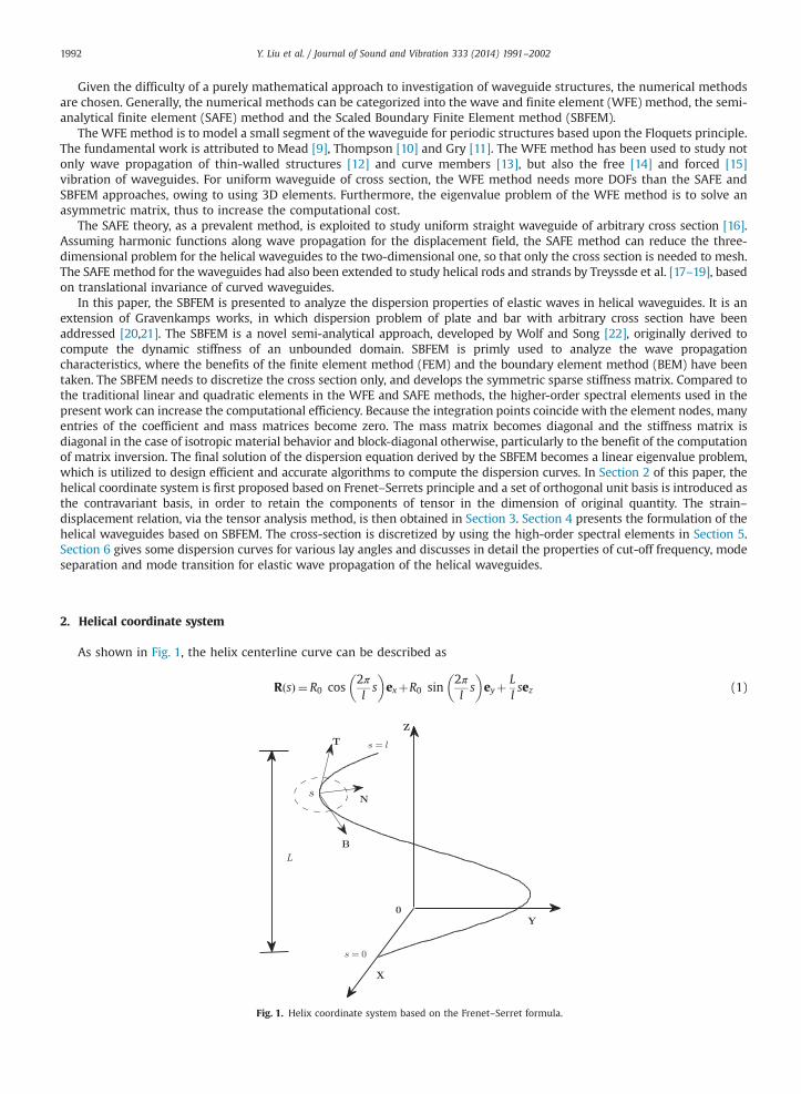
As shown in Fig. 1, the helix centerline curve can be described as

R sð Þ ¼ R0 cos2πls

� �exþR0 sin

2πls

� �eyþ

Llsez (1)

Fig. 1. Helix coordinate system based on the Frenet–Serret formula.

Y. Liu et al. / Journal of Sound and Vibration 333 (2014) 1991–2002 1993

where s is the arclength parameter, ex; ey; ez are the bases of the Cartesian coordinate, R0 is the radius of the helix, L is thepitch, l is the length of one turn of the helix. The curvature κ and the tortuosity τ of the curve defined by Eq. (1) arerespectively 4π2R2

0=l2 and 2πL=l. The unit vector tangent to the centerline is given by TðsÞ ¼ dRðsÞ=ds. The tangent, normal,

and binormal unit vectors, called TðsÞ, NðsÞ and BðsÞ, or collectively the Frenet–Serret frame, together form an orthonormalbasis spanning three-dimensional Euclidean space. Then the Frenet–Serret frame satisfies dT=ds¼ κN, dN=ds¼ τB�κT,dB=ds¼ �τN . For clarity, TðsÞ, NðsÞ and BðsÞ are expressed in the Cartesian basis as

N sð Þ ¼ 1κ

dTðsÞds

¼ � cos2πls

� �ex� sin

2πls

� �ey (2)

B sð Þ ¼ 1τ

dNðsÞds

þκT sð Þ� �

¼ Llsin

2πls

� �ey�

Llcos

2πls

� �eyþ

2πR0

lez (3)

T sð Þ ¼ dRðsÞds

¼ � 2πR0

lsin

2πls

� �exþ 2πR0

lcos

2πls

� �eyþ L

lez (4)

We establish a local coordinate system in the N–B plate. Any point in the helical coordinate can be written as a positionvector Φ:

Φðx; y; sÞ ¼ RðsÞþxNðsÞþyBðsÞ: (5)

Utilizing Frenet–Serret formula, we obtain the natural basis gi:

g1 ¼NðsÞg2 ¼ BðsÞ

g3 ¼ �τyNðsÞþτxBðsÞþð1þκyÞTðsÞ (6)

which is not holonomic. The metric tensor then follows from gij ¼ gigj, in matrix form

G¼1 0 �τy

1 0 τx

�τy τx τ2ðx2þy2Þþð1þκxÞ2

264

375: (7)

In mathematical physics, the physical components of tensor with respect to the nonholonomic basis are inconsistent withthe original dimension of physical quantities. Hence, there are inconveniences that deduce the following equation. We needto introduce a set of orthogonal unit vectors gðiÞ as the covariant basis, in order to clearly define the physical dimension oftensor fields. Here, we choose the Frenet–Serret frame as gðiÞ :

gð1Þ ¼NðsÞ; gð2Þ ¼ BðsÞ; gð3Þ ¼ TðsÞ: (8)

We find that the components in the two bases are related by the transformation

gðiÞ ¼ βijgj or gi ¼ β′ijgðjÞ ði; j¼ 1;2;3Þ (9)

where β and β′ are respectively now

β¼ 11þκx

1þκx 0 τy

0 1þκx �τx0 0 1

264

375 (10)

β′¼1 0 00 1 0

�τy τx 1þκx

264

375 (11)

The contravariant basis gi of the helical coordinate, defined by gigi ¼ δji, is given by

g1 ¼N sð Þþ τyð1þκxÞT sð Þ; g2 ¼ B sð Þ� τx

ð1þκxÞT sð Þ; g3 ¼ 1ð1þκxÞT sð Þ (12)

and the transformation between the contravariant basis and the natural basis obeys

gðiÞ ¼ β′ijgj or gi ¼ βijgðjÞ ði; j¼ 1;2;3Þ: (13)

3. The strain–displacement relation of the helical coordinate

Discussing the properties of elastic wave in the helical rod, we need only to consider small strain. The strains E can bedefined as

E¼ 1=2ð∇Uþð∇UÞT Þ (14)

Y. Liu et al. / Journal of Sound and Vibration 333 (2014) 1991–20021994

where the displacement field U is expressed in the tensor form by

U¼ uigðiÞ ¼ ungð1Þ þubgð2Þ þutgð3Þ (15)

and ∇ represents the gradient operator. Right-gradient and left-gradient of the displacement field respectively are

∇U¼ gi∂U∂xi

¼ βijgðiÞ∂U∂xi

(16)

U∇¼ ∂U∂xi

gi ¼ ∂U∂xi

βijgðiÞ: (17)

We can rewrite the second order tensor E by using the tensor form

E¼ ɛijgðiÞgðjÞ (18)

Solving the simultaneous Eqs. (14) and (15), we find that

ε¼ ½ɛnn ɛbb ɛtt 2ɛnb 2ɛnt 2ɛbt �T ¼ b1u;xþb2u;yþbsu;sþb0u (19)

where the strain tensor satisfies ɛnb ¼ ɛbn; ɛnt ¼ ɛtn; ɛtb ¼ ɛbt , and the differential operation matrices b1;b2;bs;b0 follow fromcomparison with Eq. (19) as

b1 ¼

10

00

00

00

01

τy=ð1þκxÞ0

τy=ð1þκxÞ0

0τy=ð1þκxÞ

10

26666666664

37777777775

(20)

b2 ¼

00

01

00

01

00

�τx=ð1þκxÞ0

�τx=ð1þκxÞ0

0�τx=ð1þκxÞ

01

26666666664

37777777775

(21)

bs ¼ 11þκx

00

00

00

00

00

10

10

01

00

26666666664

37777777775; b0 ¼

11þκx

00

00

00

κ

000

00

0τ

�τ

0�κ

0

26666666664

37777777775: (22)

4. Scaled boundary finite element formulation

In the SBFEM, the geometry of a helical waveguide is described by two-dimensional finite elements with localcoordinates ξ; η on the cross section and a scaled coordinate sn parallel to the helical curved direction. The coordinate sn

measures the arc length from the scaling center at infinity. The following steps are derived for one isoparametric elementto obtain the stiffness matrix of the element, which assembles to the global stiffness matrix. The geometry of a finiteelement on the cross section is represented by interpolating its nodal coordinates xi; yi using the local coordinates ξ; η:

xðξ; ηÞ ¼Niðξ; ηÞxiyðξ; ηÞ ¼Niðξ; ηÞyi (23)

with the mapping functions Niðξ; ηÞ. To transform the differential operator of Eq. (19) to the local coordinate, the coordinaterelation is required:

∂ξ∂η

" #¼ J

∂x∂y

" #; ∂s ¼ ∂sn (24)

Y. Liu et al. / Journal of Sound and Vibration 333 (2014) 1991–2002 1995

with the Jacobian matrix

J¼x;ξ x;ξy;η y;η

" #(25)

The partial derivatives x;ξ; x;η; y;ξ and y;η are calculated via Eq. (23):

x;ξ ¼Ni ;ξxi; x;η ¼Ni ;ηxi

y;ξ ¼Ni ;ξyi; y;η ¼Ni ;ηyi: (26)

Inverting Eq. (24), we obtain

∂x∂y

" #¼ 1

jJjy;η �y;ξ�x;η x;ξ

" #∂ξ∂η

" #(27)

The displacement amplitudes of one finite element on the cross section are interpolated using shape functions that areequal to the mapping functions. Hence, with the nodal displacement ui

jðsnÞ the displacements of one finite element areapproximated by

ujðξ; η; snÞ ¼Niðξ; ηÞuijðsnÞ (28)

where the subscript i¼ n; b; t denotes components with respect to N, B, T. Substituting Eq. (27) into Eq. (19), we obtain

ε¼ B1uðsnÞþBsn u ;sn ðsnÞ (29)

with

Bsn ¼ bsN (30)

B1 ¼1jJj y;ηb1�x;ηb2

� �N;ξþ

1jJj �y;ξb1þx;ξb2

� �N;ηþb0N (31)

We now consider the conditions under which time-harmonic waves may propagate in a helical rod and there is noexternal body force for studying the properties of propagation modes. The application of the Hamiltons variational principlegoverning dynamics is Z

VδεTr dV�ω2

ZVδuTρu dV ¼ 0 (32)

with

dV ¼ffiffiffiffiffiffijGj

pdx dy ds¼ jJj

ffiffiffiffiffiffijGj

pdξ dη dsn (33)

where ρ is the material density and ω is the circular frequency. Assuming an isotropic elastic material, the stress–strainrelation is written as

r¼ ½snn sbb stt snb snt sbt �T ¼ Cε (34)

where C is the constitutive matrix. Substituting Eqs. (29) and (34) into Eq. (33), we obtain

E1uðsnÞþðE2�ET2Þu ;sn ðsnÞ�E3u ;snsn ðsnÞ�ω2MuðsnÞ ¼ 0 (35)

with

M¼ZΓeNTρNjJj

ffiffiffiffiffiffijGj

pdξ dη; E1 ¼

ZΓeBT1CB1jJj

ffiffiffiffiffiffijGj

pdξ dη

E2 ¼ZΓeBT1CBsn jJj

ffiffiffiffiffiffijGj

pdξ dη; E3 ¼

ZΓeBTsnCBsn jJj

ffiffiffiffiffiffijGj

pdξ dη: (36)

For a Fourier transform of the s direction, we can obtain the displacement field depending on eiðks�ωtÞ, where k is thewavenumber along the direction. Hence, Eq. (35) can be rewritten as

E1uðsnÞþ ikðE2�ET2ÞuðsnÞ�k2E3uðsnÞ�ω2MuðsnÞ ¼ 0: (37)

Eq. (37) is the dispersion equation about the helical waveguide that can turn into a polynomial eigenvalue problem of twovariables (k,ω). For a given ω, we can easily find out that both k and �k are eigenvalues of Eq. (37), because of the symmetryof M;E1;E3 and the dissymmetry of E2�ET

2, which represent positive-going and negative-going wave types. Using theproperties of the stiffness matrix derived by the high-order spectral elements, we can simplify the final problem to ageneralized linear eigensystem:

�Aφ¼ λφ (38)

Y. Liu et al. / Journal of Sound and Vibration 333 (2014) 1991–20021996

with

A¼E�13 ET

2 �E�13

ω2M�E1þE2E�13 ET2 �E2E

�13

" #; φ¼ ½u3n; q3n�T ; λ¼ ik (39)

where u3n and q3n are respectively the nodal displacement and force vector and the subscript n is the number of nodes inthe cross section. Thus, the number of degrees of freedom (dofs) is 3n and A is a 6n� 6n matrix which has the 6neigenvalues. Due to the Hermetical properties of the eigenmatrix obtained by the SAEF method, we can easily check thatboth k and k are also eigenvalues of Eq. (39), where the superscript � refers to the complex conjugate. Purely realcorresponds to propagation modes, without attenuation under no damp, while purely imaginary wavenumber is notconsidered, which is regarded as the perturbance called as evanescent modes. All other with full complex eigenvaluerepresents inhomogenous modes, decaying exponentially in the propagation direction.

For the modes ðk; uÞ, the phase velocity vp is defined by ω=ReðkÞ and the attenuation coefficient β is ImðkÞ, where Re andIm represent real part and imaginary part of the complex, respectively. The cross section energy velocity of the time averageover one period is written as follows [23]:

ve ¼Re

RΓeP � gð3Þ ds

� �Re

RΓeE ds

� � : (40)

In the nondissipative system, the group velocity vg ¼ ∂ω=∂k is equivalent to the energy velocity (as opposed to thedissipative system under which the group velocity is not generally valid).

RΓeP � gð3Þ ds is the kinetic energy of the cross

section and time average in the propagation direction, where P is the Poynting vector defined by P ¼ 0:5sijgðiÞgðjÞ � _u jgðjÞ.RΓeE ds is the summation of the kinetic and potential energies. We haveZ

ΓeP � gð3Þ ds¼

Zs

iωn

2uT 1þκxð ÞbT

s C b1þ ikbsð Þu� �

ds¼ ωn

2Im u

TET4þ iknE5

� �u

� �(41)

ZΓeE ds¼ ω2

4u

TMuþ 1

4u

TE1þ ik E2�ET

2

� �þk2E3

� �u (42)

with

E4 ¼ZΓeBT1CBsn ð1þκxÞjJj

ffiffiffiffiffiffijGj

pdξ dη (43)

E5 ¼ZΓeð1þκxÞBT

snCBsn jJjffiffiffiffiffiffijGj

pdξ dη (44)

5. Discretization

Comparing the traditional finite element methods using Linear Lagrangian element basis function with uniformdiscretization (equidistant element nodes), the spectral methods utilizing the Gauss–Lobatto–Legendre element can usuallyachieve higher accuracy and demand less memory. The local coordinates ξ; η of the nodes for the two-dimensional spectralelement are defined by the roots of the following polynomial [24]:

ð1�ξ2ÞP′MðξÞ ¼ 0

ð1�η2ÞP′MðηÞ ¼ 0

((45)

and weights obey

wi ¼1

MðMþ1ÞðPMðξiÞÞ2ξia71ð Þ

wi ¼1

MðMþ1Þ ξi ¼ 71ð Þ (46)

where PM is the Legendre polynomial of order M, such as the sixth-order element shown by Fig. 2(a) whose grid points andweights are illustrated by Table 1. Lagrange interpolation polynomial of nonequidistant nodes can be written down directly as

Nα ξð Þ ¼ ∏nξ þ1

i ¼ 1;iaα

ξ�ξαξi�ξα

i¼ 1;2… nξþ1� �� �

(47)

where nξ is the number of nodes in the ξ direction. In two dimensions, the shape functions can be achieved by simple products ofLagrange polynomial in the two coordinates:

For the integral computation of Eq. (36), the properties of the Gauss–Lobatto–Legendre element, including thesuperposition between the integration points and the nodes and the Kronecher delta of the interpolation basis function,contribute to many off-diagonal entries of the matrices to be zero in Eq. (36), so that the diagonalization of the matrices M,

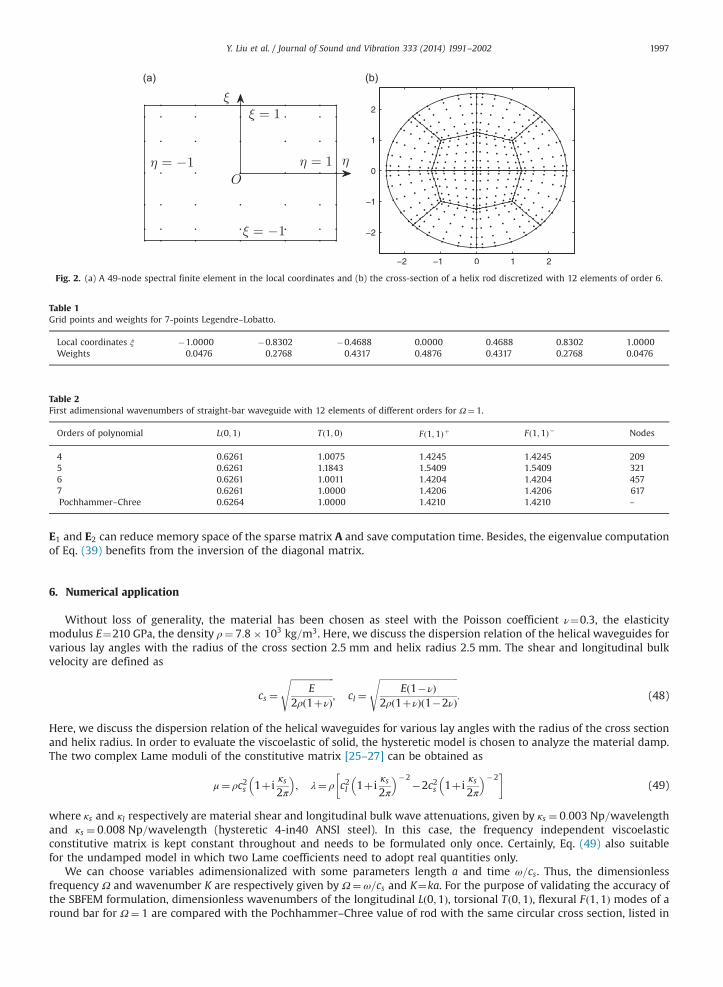
Fig. 2. (a) A 49-node spectral finite element in the local coordinates and (b) the cross-section of a helix rod discretized with 12 elements of order 6.

Table 1Grid points and weights for 7-points Legendre–Lobatto.

Local coordinates ξ �1.0000 �0.8302 �0.4688 0.0000 0.4688 0.8302 1.0000Weights 0.0476 0.2768 0.4317 0.4876 0.4317 0.2768 0.0476

Table 2First adimensional wavenumbers of straight-bar waveguide with 12 elements of different orders for Ω¼ 1.

Orders of polynomial Lð0;1Þ Tð1;0Þ Fð1;1Þþ Fð1;1Þ� Nodes

4 0.6261 1.0075 1.4245 1.4245 2095 0.6261 1.1843 1.5409 1.5409 3216 0.6261 1.0011 1.4204 1.4204 4577 0.6261 1.0000 1.4206 1.4206 617Pochhammer–Chree 0.6264 1.0000 1.4210 1.4210 –

Y. Liu et al. / Journal of Sound and Vibration 333 (2014) 1991–2002 1997

E1 and E2 can reduce memory space of the sparse matrix A and save computation time. Besides, the eigenvalue computationof Eq. (39) benefits from the inversion of the diagonal matrix.

6. Numerical application

Without loss of generality, the material has been chosen as steel with the Poisson coefficient ν¼0.3, the elasticitymodulus E¼210 GPa, the density ρ¼ 7:8� 103 kg=m3. Here, we discuss the dispersion relation of the helical waveguides forvarious lay angles with the radius of the cross section 2.5 mm and helix radius 2.5 mm. The shear and longitudinal bulkvelocity are defined as

cs ¼ffiffiffiffiffiffiffiffiffiffiffiffiffiffiffiffiffiffiffi

E2ρð1þνÞ

s; cl ¼

ffiffiffiffiffiffiffiffiffiffiffiffiffiffiffiffiffiffiffiffiffiffiffiffiffiffiffiffiffiffiffiffiffiffiEð1�νÞ

2ρð1þνÞð1�2νÞ

s: (48)

Here, we discuss the dispersion relation of the helical waveguides for various lay angles with the radius of the cross sectionand helix radius. In order to evaluate the viscoelastic of solid, the hysteretic model is chosen to analyze the material damp.The two complex Lame moduli of the constitutive matrix [25–27] can be obtained as

μ¼ ρc2s 1þ iκs2π

� �; λ¼ ρ c2l 1þ i

κs2π

� ��2�2c2s 1þ i

κs2π

� ��2

(49)

where κs and κl respectively are material shear and longitudinal bulk wave attenuations, given by κs ¼ 0:003 Np=wavelengthand κs ¼ 0:008 Np=wavelength (hysteretic 4-in40 ANSI steel). In this case, the frequency independent viscoelasticconstitutive matrix is kept constant throughout and needs to be formulated only once. Certainly, Eq. (49) also suitablefor the undamped model in which two Lame coefficients need to adopt real quantities only.

We can choose variables adimensionalized with some parameters length a and time ω=cs. Thus, the dimensionlessfrequency Ω and wavenumber K are respectively given by Ω¼ ω=cs and K¼ka. For the purpose of validating the accuracy ofthe SBFEM formulation, dimensionless wavenumbers of the longitudinal Lð0;1Þ, torsional Tð0;1Þ, flexural Fð1;1Þ modes of around bar for Ω¼ 1 are compared with the Pochhammer–Chree value of rod with the same circular cross section, listed in

Fig. 3. Spectrum curves for Ω ranging from 0 and 5 without material damp. Left: Cylinder. Right: Helical lay angle φ¼ 7:51 . Blue lines (the positive numberof Y-axis represents ReðkaÞ): propagate modes obtained with the SBFEM. Olive lines: Propagate modes obtained with the SAFE method. Wine lines (thenegative number of Y-axis represents ImðkaÞ): inhomogeneous modes. Cyan lines: Evanescent modes. (a) Frequency spectrum for cylinder and(b) frequency spectrum for φ¼ 7:51. (For interpretation of the references to color in this figure caption, the reader is referred to the web version of thisarticle.)

Fig. 4. Energy velocity and attenuation curves for Ω ranging from 0 and 5. Left: cylinder. Right: helical 7.51. Red and blue lines of (a) and (b) respectivelypresent the energy velocity curve the undamped and damping media. (a) Energy velocity curves for θ¼ 01, (b) energy velocity curves for θ¼ 7:51,(c) attenuation curves for θ¼ 01, and (d) attenuation curves for θ¼ 7:51. (For interpretation of the references to color in this figure caption, the reader isreferred to the web version of this article.)

Y. Liu et al. / Journal of Sound and Vibration 333 (2014) 1991–20021998

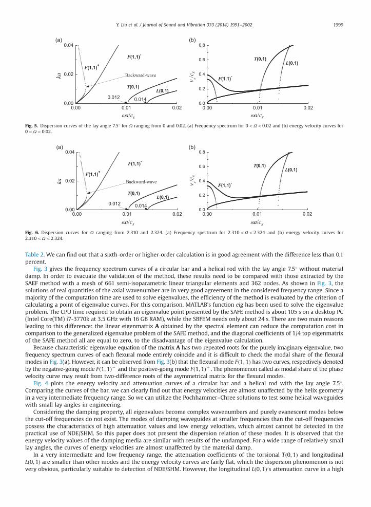
Fig. 5. Dispersion curves of the lay angle 7.51 for Ω ranging from 0 and 0.02. (a) Frequency spectrum for 0oΩo0:02 and (b) energy velocity curves for0oΩo0:02.

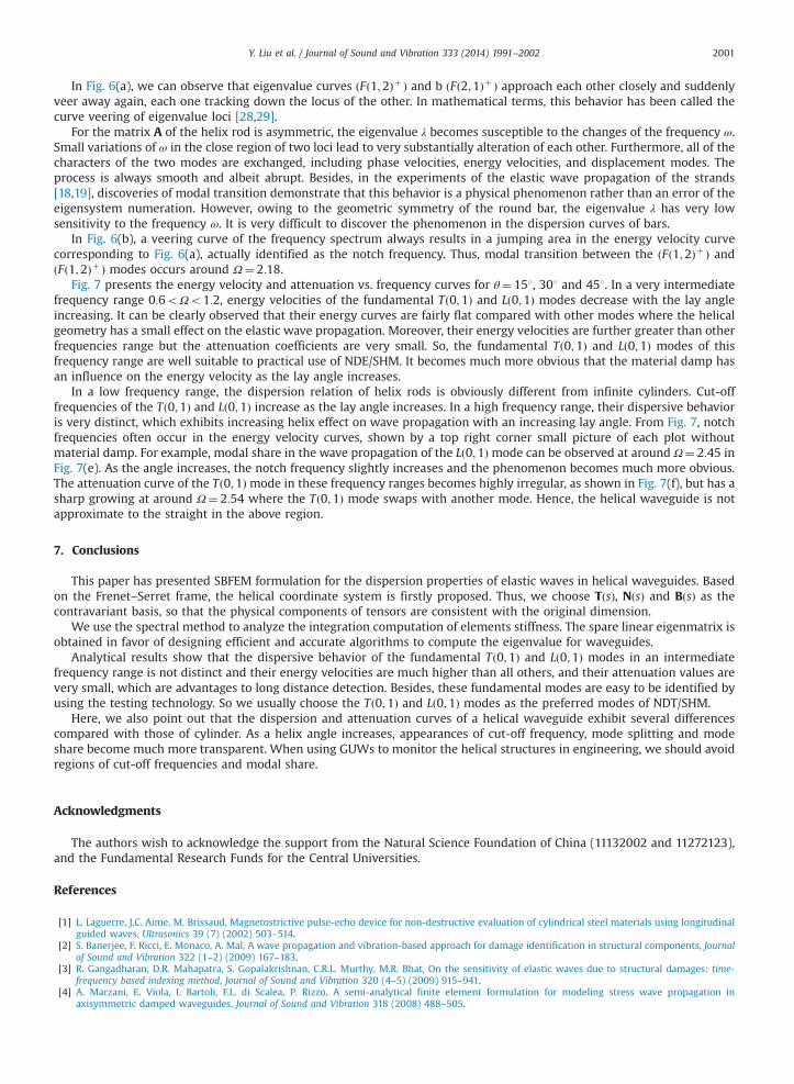
Fig. 6. Dispersion curves for Ω ranging from 2.310 and 2.324. (a) Frequency spectrum for 2:310oΩo2:324 and (b) energy velocity curves for2:310oΩo2:324.

Y. Liu et al. / Journal of Sound and Vibration 333 (2014) 1991–2002 1999

Table 2. We can find out that a sixth-order or higher-order calculation is in good agreement with the difference less than 0.1percent.

Fig. 3 gives the frequency spectrum curves of a circular bar and a helical rod with the lay angle 7.51 without materialdamp. In order to evacuate the validation of the method, these results need to be compared with those extracted by theSAEF method with a mesh of 661 semi-isoparametric linear triangular elements and 362 nodes. As shown in Fig. 3, thesolutions of real quantities of the axial wavenumber are in very good agreement in the considered frequency range. Since amajority of the computation time are used to solve eigenvalues, the efficiency of the method is evaluated by the criterion ofcalculating a point of eigenvalue curves. For this comparison, MATLAB's function eig has been used to solve the eigenvalueproblem. The CPU time required to obtain an eigenvalue point presented by the SAFE method is about 105 s on a desktop PC(Intel Core(TM) i7-3770k at 3.5 GHz with 16 GB RAM), while the SBFEM needs only about 24 s. There are two main reasonsleading to this difference: the linear eigenmatrix A obtained by the spectral element can reduce the computation cost incomparison to the generalized eigenvalue problem of the SAFE method, and the diagonal coefficients of 1/4 top eigenmatrixof the SAFE method all are equal to zero, to the disadvantage of the eigenvalue calculation.

Because characteristic eigenvalue equation of the matrix A has two repeated roots for the purely imaginary eigenvalue, twofrequency spectrum curves of each flexural mode entirely coincide and it is difficult to check the modal share of the flexuralmodes in Fig. 3(a). However, it can be observed from Fig. 3(b) that the flexural mode Fð1;1Þ has two curves, respectively denotedby the negative-going mode Fð1;1Þ� and the positive-going mode Fð1;1Þþ . The phenomenon called as modal share of the phasevelocity curve may result from two-difference roots of the asymmetrical matrix for the flexural modes.

Fig. 4 plots the energy velocity and attenuation curves of a circular bar and a helical rod with the lay angle 7.51.Comparing the curves of the bar, we can clearly find out that energy velocities are almost unaffected by the helix geometryin a very intermediate frequency range. So we can utilize the Pochhammer–Chree solutions to test some helical waveguideswith small lay angles in engineering.

Considering the damping property, all eigenvalues become complex wavenumbers and purely evanescent modes belowthe cut-off frequencies do not exist. The modes of damping waveguides at smaller frequencies than the cut-off frequenciespossess the characteristics of high attenuation values and low energy velocities, which almost cannot be detected in thepractical use of NDE/SHM. So this paper does not present the dispersion relation of these modes. It is observed that theenergy velocity values of the damping media are similar with results of the undamped. For a wide range of relatively smalllay angles, the curves of energy velocities are almost unaffected by the material damp.

In a very intermediate and low frequency range, the attenuation coefficients of the torsional Tð0;1Þ and longitudinalLð0;1Þ are smaller than other modes and the energy velocity curves are fairly flat, which the dispersion phenomenon is notvery obvious, particularly suitable to detection of NDE/SHM. However, the longitudinal Lð0;1Þ′s attenuation curve in a high

Fig. 7. Energy velocity and attenuation curves for θ¼ 151;301 and 451 with Ω ranging from 0 and 5. Red and blue lines of (a), (b) and (c) respectivelypresent energy velocity curves of the undamped and damping media. (a) Energy velocity curves for θ¼ 151, (b) attenuation curves for θ¼ 151, (c) energyvelocity curves for θ¼ 301, (d) attenuation curves for θ¼ 301, (e) energy velocity curves for θ¼ 451, and (f) attenuation curves for θ¼ 451. (Forinterpretation of the references to color in this figure caption, the reader is referred to the web version of this article.)

Y. Liu et al. / Journal of Sound and Vibration 333 (2014) 1991–20022000

frequency range becomes acute variety whose values are much greater than all other modes, which is disadvantage to thelong-distance detection of NDE/SHM.

Fig. 5(a) gives the frequency spectrum of the helical rod with the lay angle 7.51 in a low frequency range 0oΩo0:02. Wecan clearly check that the longitudinal Lð0;1Þ mode and the torsional Tð0;1Þ mode are respectively cut-off near Ω¼ 0:014and Ω¼ 0:012. Thus, back-ward wave occurs in the range 0oΩo0:005 of the flexural Fð1;1Þþ where the direction of theenergy velocity propagation is opposite to the phase velocity.

Y. Liu et al. / Journal of Sound and Vibration 333 (2014) 1991–2002 2001

In Fig. 6(a), we can observe that eigenvalue curves ðFð1;2Þþ Þ and b ðFð2;1Þþ Þ approach each other closely and suddenlyveer away again, each one tracking down the locus of the other. In mathematical terms, this behavior has been called thecurve veering of eigenvalue loci [28,29].

For the matrix A of the helix rod is asymmetric, the eigenvalue λ becomes susceptible to the changes of the frequency ω.Small variations of ω in the close region of two loci lead to very substantially alteration of each other. Furthermore, all of thecharacters of the two modes are exchanged, including phase velocities, energy velocities, and displacement modes. Theprocess is always smooth and albeit abrupt. Besides, in the experiments of the elastic wave propagation of the strands[18,19], discoveries of modal transition demonstrate that this behavior is a physical phenomenon rather than an error of theeigensystem numeration. However, owing to the geometric symmetry of the round bar, the eigenvalue λ has very lowsensitivity to the frequency ω. It is very difficult to discover the phenomenon in the dispersion curves of bars.

In Fig. 6(b), a veering curve of the frequency spectrum always results in a jumping area in the energy velocity curvecorresponding to Fig. 6(a), actually identified as the notch frequency. Thus, modal transition between the ðFð1;2Þþ Þ andðFð1;2Þþ Þ modes occurs around Ω¼ 2:18.

Fig. 7 presents the energy velocity and attenuation vs. frequency curves for θ¼ 151, 301 and 451. In a very intermediatefrequency range 0:6oΩo1:2, energy velocities of the fundamental Tð0;1Þ and Lð0;1Þ modes decrease with the lay angleincreasing. It can be clearly observed that their energy curves are fairly flat compared with other modes where the helicalgeometry has a small effect on the elastic wave propagation. Moreover, their energy velocities are further greater than otherfrequencies range but the attenuation coefficients are very small. So, the fundamental Tð0;1Þ and Lð0;1Þ modes of thisfrequency range are well suitable to practical use of NDE/SHM. It becomes much more obvious that the material damp hasan influence on the energy velocity as the lay angle increases.

In a low frequency range, the dispersion relation of helix rods is obviously different from infinite cylinders. Cut-offfrequencies of the Tð0;1Þ and Lð0;1Þ increase as the lay angle increases. In a high frequency range, their dispersive behavioris very distinct, which exhibits increasing helix effect on wave propagation with an increasing lay angle. From Fig. 7, notchfrequencies often occur in the energy velocity curves, shown by a top right corner small picture of each plot withoutmaterial damp. For example, modal share in the wave propagation of the Lð0;1Þ mode can be observed at around Ω¼ 2:45 inFig. 7(e). As the angle increases, the notch frequency slightly increases and the phenomenon becomes much more obvious.The attenuation curve of the Tð0;1Þmode in these frequency ranges becomes highly irregular, as shown in Fig. 7(f), but has asharp growing at around Ω¼ 2:54 where the Tð0;1Þ mode swaps with another mode. Hence, the helical waveguide is notapproximate to the straight in the above region.

7. Conclusions

This paper has presented SBFEM formulation for the dispersion properties of elastic waves in helical waveguides. Basedon the Frenet–Serret frame, the helical coordinate system is firstly proposed. Thus, we choose TðsÞ, NðsÞ and BðsÞ as thecontravariant basis, so that the physical components of tensors are consistent with the original dimension.

We use the spectral method to analyze the integration computation of elements stiffness. The spare linear eigenmatrix isobtained in favor of designing efficient and accurate algorithms to compute the eigenvalue for waveguides.

Analytical results show that the dispersive behavior of the fundamental Tð0;1Þ and Lð0;1Þ modes in an intermediatefrequency range is not distinct and their energy velocities are much higher than all others, and their attenuation values arevery small, which are advantages to long distance detection. Besides, these fundamental modes are easy to be identified byusing the testing technology. So we usually choose the Tð0;1Þ and Lð0;1Þ modes as the preferred modes of NDT/SHM.

Here, we also point out that the dispersion and attenuation curves of a helical waveguide exhibit several differencescompared with those of cylinder. As a helix angle increases, appearances of cut-off frequency, mode splitting and modeshare become much more transparent. When using GUWs to monitor the helical structures in engineering, we should avoidregions of cut-off frequencies and modal share.

Acknowledgments

The authors wish to acknowledge the support from the Natural Science Foundation of China (11132002 and 11272123),and the Fundamental Research Funds for the Central Universities.

References

[1] L. Laguerre, J.C. Aime, M. Brissaud, Magnetostrictive pulse-echo device for non-destructive evaluation of cylindrical steel materials using longitudinalguided waves, Ultrasonics 39 (7) (2002) 503–514.

[2] S. Banerjee, F. Ricci, E. Monaco, A. Mal, A wave propagation and vibration-based approach for damage identification in structural components, Journalof Sound and Vibration 322 (1–2) (2009) 167–183.

[3] R. Gangadharan, D.R. Mahapatra, S. Gopalakrishnan, C.R.L. Murthy, M.R. Bhat, On the sensitivity of elastic waves due to structural damages: time-frequency based indexing method, Journal of Sound and Vibration 320 (4–5) (2009) 915–941.

[4] A. Marzani, E. Viola, I. Bartoli, F.L. di Scalea, P. Rizzo, A semi-analytical finite element formulation for modeling stress wave propagation inaxisymmetric damped waveguides, Journal of Sound and Vibration 318 (2008) 488–505.

Y. Liu et al. / Journal of Sound and Vibration 333 (2014) 1991–20022002

[5] H. Kwun, K.A. Bartels, J.J. Hanley, Effects of tensile loading on the properties of elastic-wave propagation in a strand, Acoustical Society of America 103(1998) 3370–3375.

[6] P. Rizzo, F.L. di Scalea, Wave propagation in multi-wire strands by wavelet-based laser ultrasound, Experimental Mechanics 44 (4) (2004) 407–415.[7] A. Baltazar, C.D. Hernandez-Salazar, B. Manzanares-Martinez, Study of wave propagation in a multiwire cable to determine structural damage, NDT &

E International 43 (2010) 726–732.[8] S. Chaki, G. Bourse, Guided ultrasonic waves for non-destructive monitoring of the stress levels in prestressed steel strands, Ultrasonics 49 (2) (2009)

162–171.[9] D.M. Mead, Wave propagation in continuous periodic structures: research contributions from Southampton, 1964–1995, Journal of Sound and Vibration

190 (1996) 495–524.[10] L. Gry, C. Gontier, Dynamic modelling of railway track: a periodic model based on a generalized beam formulation, Journal of Sound and Vibration 199

(1997) 531–558.[11] D. Thompson, Wheel-rail noise generation, Part i: introduction and interaction model, Journal of Sound and Vibration 161 (1993) 387–400.[12] L. Houillon, M. Ichchou, L. Jezequel, Wave motion in thin-walled structures, Journal of Sound and Vibration 281 (3–5) (2005) 483–507.[13] W. Zhou, M. Ichchou, Wave propagation in mechanical waveguide with curved members using wave finite element solution, Computer Methods in

Applied Mechanics and Engineering 199 (33–36) (2010) 2099–2109.[14] J.-M. Mencik, A model reduction strategy for computing the forced response of elastic waveguides using the wave finite element method, Computer

Methods in Applied Mechanics and Engineering 229 (2012) 68–86.[15] Y. Waki, B. Mace, M. Brennan, Numerical issues concerning the wave and finite element method for free and forced vibrations of waveguides, Journal of

Sound and Vibration 327 (1–2) (2009) 92–108.[16] T. Hayashi, W.-J. Song, J.L. Rose, Guided wave dispersion curves for a bar with an arbitrary cross-section, a rod and rail example, Ultrasonics 41 (3)

(2003) 175–183.[17] F. Treyssède, Numerical investigation of elastic modes of propagation in helical waveguides, The Journal of the Acoustical Society of America 121 (6)

(2007) 3398–3408.[18] F. Treyssède, L. Laguerre, Investigation of elastic modes propagating in multi-wire helical waveguides, Journal of Sound and Vibration 329 (10) (2010)

1702–1716.[19] F. Treyssède, A. Frikha, P. Cartraud, Mechanical modeling of helical structures accounting for translational invariance. Part 2: guided wave propagation

under axial loads, International Journal of Solids and Structures 50 (9) (2013) 1383–1393.[20] H. Gravenkamp, C. Song, J. Prager, A numerical approach for the computation of dispersion relations for plate structures using the Scaled Boundary

Finite Element method, Journal of Sound and Vibration 331 (11) (2012) 2543–2557.[21] H. Gravenkamp, H. Man, C. Song, J. Prager, The computation of dispersion relations for three-dimensional elastic waveguides using the scaled

boundary finite element method, Journal of Sound and Vibration 332 (15) (2013) 3756–3771.[22] J.P. Wolf, C. Song, Finite-Element Modelling of Unbounded Media, Wiley Chichester, 1996.[23] A. Bernard, M.J.S. Lowe, M. Deschamps, Guided waves energy velocity in absorbing and non-absorbing plates, The Journal of the Acoustical Society of

America 110 (1) (2001) 186–196.[24] J.P. Boyd, Chebyshev and Fourier Spectral Methods, Courier Dover Publications, 2001.[25] I. Bartoli, A. Marzani, F. Lanza di Scalea, E. Viola, Modeling wave propagation in damped waveguides of arbitrary cross-section, Journal of Sound and

Vibration 295 (3–5) (2006) 685–707.[26] A. Marzani, E. Viola, I. Bartoli, F. Lanza di Scalea, P. Rizzo, A semi-analytical finite element formulation for modeling stress wave propagation in

axisymmetric damped waveguides, Journal of Sound and Vibration 318 (3) (2008) 488–505.[27] A. Marzani, Time-transient response for ultrasonic guided waves propagating in damped cylinders, International Journal of Solids and Structures 45

(25–26) (2008) 6347–6368, http://dx.doi.org/10.1016/j.ijsolstr.2008.07.028.[28] X. Chen, A. Kareem, Curve veering of eigenvalue loci of bridges with aeroelastic effects, Journal of Engineering Mechanics 129 (2) (2003) 146–159.[29] B.R. Mace, E. Manconi, Wave motion and dispersion phenomena: veering, locking and strong coupling effects, The Journal of the Acoustical Society of

America 131 (2) (2012) 1015–1028.