Numerical Estimation of Marcum’s Q-Function

using Monte Carlo Approximation Schemes

Graham V. Weinberg and Louise Panton

Electronic Warfare and Radar DivisionDefence Science and Technology Organisation

DSTO–RR–0311

ABSTRACT

The Marcum Q-Function is an important tool in the study of radar detec-tion probabilities in Gaussian clutter and noise. Due to the fact that it isan intractable integral, much research has focused on finding good numeri-cal approximations for it. Such approximations include numerical integrationtechniques, such as adaptive Simpson quadrature, and Taylor series approxi-mations, induced by the modified Bessel function of order zero, which appearsin the integrand. One technique which has not been explored in the literatureis the sampling-based Monte Carlo approach. Part of the reason for this is thatthe integral representation of the Marcum Q-Function is not in the most suit-able form for Monte Carlo methods. Using some recently derived techniques,we construct a number of sampling-based estimators of this function, and weconsider their relative merits.

APPROVED FOR PUBLIC RELEASE

DSTO–RR–0311

Published by

Defence Science and Technology OrganisationPO Box 1500Edinburgh, South Australia, Australia 5111

Telephone: (08) 8259 5555Facsimile: (08) 8259 6567

c© Commonwealth of Australia 2006AR No. AR-013-613April, 2006

APPROVED FOR PUBLIC RELEASE

ii

DSTO–RR–0311

Numerical Estimation of Marcum’s Q-Function using MonteCarlo Approximation Schemes

EXECUTIVE SUMMARY

Radar detector performance and analysis are issues of paramount importance to the modusoperandi of Electronic Warfare and Radar Division’s Radar Modelling and Analysis Group.The research presented here is the practical extension of that which has appeared in arecent research report by the first author [DSTO-RR-0304, ‘Stochastic Representations ofthe Marcum Q-Function and Associated Radar Detection Probabilities’]. Hence it is insupport of the ongoing long range research efforts for AIR 04/206. The purpose of this taskis to provide the Royal Australian Air Force with technical advice on the performance of theElta EL/M-2022 maritime radar, which is used in the AP-3C Orion fleet. Key performancemeasures of a radar include probabilities of false alarm and detection. The work presentedhere is concerned with the efficient estimation of a specific radar detection probability,known as Marcum’s Q-function. This corresponds to the detection probability of a targetin Gaussian clutter and noise, and so is a fundamental model in radar detection theory.This probability has been of interest to DSTO’s research interests since the 1970s, throughTask DST 74/130, which required the efficient estimation of the Marcum Q-Function.

In contrast to the techniques currently used in the radar literature, we investigate theapplication of Monte Carlo sampling methods to estimate this detection probability. Suchmethods have been investigated by the first author, in a number of DSTO reports, alsoin support of AIR 04/206 and its precursor AIR 01/217. The Marcum Q-Function doesnot prima facie suggest that Monte Carlo techniques would be suitable. New discoveries,through stochastic representations of the Marcum Q-function, have indicated that MonteCarlo techniques may be useful tools in the estimation of detection probabilities. We thusinvestigate whether these stochastic representations admit useful and efficient Monte Carloestimators of the Marcum Q-Function.

iii

DSTO–RR–0311

iv

DSTO–RR–0311

Authors

Graham V. WeinbergElectronic Warfare and Radar Division

Graham V. Weinberg, Ph.D. is a specialist in mathematicalanalysis and applied probability, and is a graduate of The Uni-versity of Melbourne. His research interests encompass the ar-eas of probability approximations and radar detection.

Louise PantonDSTO Summer Vacation Scholarship Program 2005/2006

Louise Panton is a final year Telecommunications Engineeringand Mathematics and Computer Science degree student at theUniversity of Adelaide, working at DSTO on a Summer Vaca-tion Scholarship.

v

DSTO–RR–0311

vi

DSTO–RR–0311

Contents

Glossary xiii

1 The Marcum Q-Function 1

1.1 The Standard Marcum Q-Function . . . . . . . . . . . . . . . . . . . . . . 1

1.2 Estimating the Marcum Q-Function . . . . . . . . . . . . . . . . . . . . . 2

1.3 Monte Carlo Methods . . . . . . . . . . . . . . . . . . . . . . . . . . . . . 2

1.4 Contributions of this Report . . . . . . . . . . . . . . . . . . . . . . . . . 3

2 Representations of the Marcum Q-Function 5

2.1 A General Result: Theorem 1 . . . . . . . . . . . . . . . . . . . . . . . . . 5

3 Monte Carlo Estimators of the Marcum Q-Function 9

3.1 Discrete Estimators . . . . . . . . . . . . . . . . . . . . . . . . . . . . . . 9

3.1.1 A Standard Monte Carlo Estimator . . . . . . . . . . . . . . . . . 9

3.1.2 A Poisson-Based Sampling Estimator: Ξ1 . . . . . . . . . . . . . 10

3.1.3 An Importance Sampling Estimator: Ξ2 . . . . . . . . . . . . . . 12

3.2 Continuous Estimators . . . . . . . . . . . . . . . . . . . . . . . . . . . . . 14

3.2.1 Estimator Based on Original Marcum Q-Function Integral: Ξ3 . . 15

3.2.2 An Estimator Based on Theorem 1 Part (iii), with Uniform Sam-pling Distribution: Ξ4 . . . . . . . . . . . . . . . . . . . . . . . . 16

3.2.3 An Estimator Based upon Theorem 1, Part (iv) using a UniformSampling Distribution: Ξ5 . . . . . . . . . . . . . . . . . . . . . . 17

3.2.4 Estimator Based upon Theorem 1, Part (iii) with Truncated Ex-ponential Sampling Distribution: Ξ6 . . . . . . . . . . . . . . . . 18

3.2.5 An Estimator Based upon Part (iv) of Theorem 1 with TruncatedExponential Sampling Distribution: Ξ7 . . . . . . . . . . . . . . . 18

4 Performance and Analysis of Estimators 20

vii

DSTO–RR–0311

4.1 Simulation Gains . . . . . . . . . . . . . . . . . . . . . . . . . . . . . . . . 20

4.2 Numerical Results . . . . . . . . . . . . . . . . . . . . . . . . . . . . . . . 21

5 Conclusions 23

6 Acknowledgements 23

References 24

Appendix A: Some Properties of Statistical Means and Variances 27

Appendix B: Generation of Realisations of Random Variables 29

Appendix C: Simulation Gains 31

Appendix D: Tables of Numerical Results 37

viii

DSTO–RR–0311

Figures

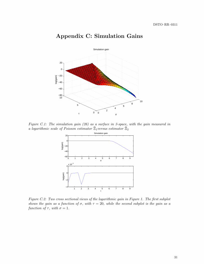
C.1 The simulation gain (26) as a surface in 3-space, with the gain measured ina logarithmic scale of Poisson estimator Ξ1versus estimator Ξ2 . . . . . . . . 31

C.2 Two cross sectional views of the logarithmic gain in Figure 1. The first subplotshows the gain as a function of σ, with τ = 20, while the second subplot isthe gain as a function of τ , with σ = 1. . . . . . . . . . . . . . . . . . . . . . . 31

C.3 The simulation gain (26) as a surface in 3-space, with the gain measured ina logarithmic scale of estimator Ξ4 versus Poisson estimator Ξ1 . . . . . . . . 32

C.4 Two cross sectional views of the logarithmic gain in Figure 3. The first subplotshows the gain as a function of σ, with τ = 20, while the second subplot isthe gain as a function of τ , with σ = 20. . . . . . . . . . . . . . . . . . . . . . 32

C.5 The simulation gain (26) as a surface in 3-space, with the gain measured ina logarithmic scale of estimator Ξ5 versus Poisson estimator Ξ1 . . . . . . . . 33

C.6 Two cross sectional views of the logarithmic gain in Figure 5. The first subplotshows the gain as a function of σ, with τ = 16, while the second subplot isthe gain as a function of τ , with σ = 1. . . . . . . . . . . . . . . . . . . . . . . 33

C.7 The simulation gain (26) as a surface in 3-space, with the gain measured ina logarithmic scale of estimator Ξ6 versus Poisson estimator Ξ1 . . . . . . . . 34

C.8 Two cross sectional views of the logarithmic gain in Figure 7. The first subplotshows the gain as a function of σ, with τ = 16, while the second subplot isthe gain as a function of τ , with σ = 1. . . . . . . . . . . . . . . . . . . . . . . 34

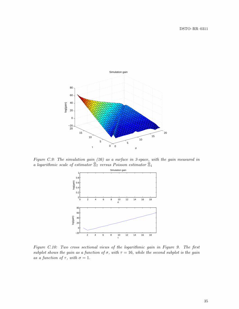
C.9 The simulation gain (26) as a surface in 3-space, with the gain measured ina logarithmic scale of estimator Ξ7 versus Poisson estimator Ξ1 . . . . . . . . 35

C.10 Two cross sectional views of the logarithmic gain in Figure 9. The first subplotshows the gain as a function of σ, with τ = 16, while the second subplot isthe gain as a function of τ , with σ = 1. . . . . . . . . . . . . . . . . . . . . . . 35

ix

DSTO–RR–0311

x

DSTO–RR–0311

Tables

D.1 A selection of estimates of ρ(σ, τ), based on a partial sum of 100 terms usingEquation (56). For each (σ, τ) pair, an estimate is compared to one obtainedby Adaptive Simpson Quadrature (ASQ), with a tolerance of 10−8. ε1 is theabsolute error between the ASQ estimate, and that based upon Equation (56). 37

D.2 Estimates of ρ(σ, τ), based upon the estimator Ξ1. For each (σ, τ) pair, anestimate is compared to one obtained by ASQ, with a tolerance of 10−8. ε1is the absolute error between the exact result and Ξ1. . . . . . . . . . . . . . 38

D.3 Estimates of ρ(σ, τ), based upon the estimator Ξ3. For each (σ, τ) pair, anestimate is compared to one obtained by ASQ, with a tolerance of 10−8. ε1is the absolute error between the ASQ estimate and Ξ3. . . . . . . . . . . . . 39

D.4 A selection of estimates of ρ(σ, τ), based upon the estimators Ξ4 and Ξ6. Foreach (σ, τ) pair, an estimate is compared to one obtained by ASQ, with atolerance of 10−8. Both ε1 and ε2 are the absolute error between the ASQestimate and Ξ4 and Ξ6 respectively. The first half of the table sets N = 103

while the second sets N = 104. . . . . . . . . . . . . . . . . . . . . . . . . . . 40

D.5 Based upon the estimators Ξ4 and Ξ6, a selection of estimates of ρ(σ, τ). Foreach (σ, τ) pair, an estimate is compared to one obtained by ASQ, with atolerance of 10−8. Both ε1 and ε2 are the absolute error between the ASQestimate and Ξ4 and Ξ6 respectively. The first half of the table sets N = 105,second sets N = 106. . . . . . . . . . . . . . . . . . . . . . . . . . . . . . . . . 41

D.6 Estimates of ρ(σ, τ), based upon the estimators Ξ5 and Ξ7. For each (σ, τ)pair, an estimate is compared to one obtained by ASQ, with a tolerance of10−8. Both ε1 and ε2 are the absolute error between the ASQ estimate andΞ5 and Ξ7 respectively. The first half of the table sets N = 103, second setsN = 104. . . . . . . . . . . . . . . . . . . . . . . . . . . . . . . . . . . . . . . . 42

D.7 A selection of estimates of ρ(σ, τ), based upon the estimators Ξ5 and Ξ7. Foreach (σ, τ) pair, an estimate is compared to one obtained by ASQ, with atolerance of 10−8. Both ε1 and ε2 are the absolute error between the ASQestimate and Ξ5 and Ξ7 respectively. The first half of the table sets N = 105,second sets N = 106. . . . . . . . . . . . . . . . . . . . . . . . . . . . . . . . . 43

D.8 The first half of the table is based upon the Uniform estimators of Theorem1 Part (iii), Ξ4 and Theorem 1 Part (iv), Ξ5. The second half of the tableis based upon the exponential estimators of Theorem 1 Part (iii), Ξ6 andTheorem 1 Part (iv), Ξ7, giving a selection of estimates of ρ(σ, τ), N = 106.For each (σ, τ) pair, an estimate is compared to one obtained by ASQ, witha tolerance of 10−8. . . . . . . . . . . . . . . . . . . . . . . . . . . . . . . . . . 44

xi

DSTO–RR–0311

xii

DSTO–RR–0311

Glossary

Fundamental Symbols

IN Natural numbers 0, 1, 2, . . ..

IR Real numbers.

IR+ Positive real numbers.

IP Probability.

IE Statistical expectation.

VV Statistical variance.

II Indicator function: II[x ∈ A] =

1 if x ∈ A;0 otherwise.

:= Defined to be.

≈ Approximately equal to.

d= Equality in distribution: X d= Y is equivalent to IP(X ∈ A) = IP(Y ∈ A) for all sets A.

σ Signal to noise ratio (SNR).

τ Detection threshold.

Ξ An estimator.

a ∧ b Minimum of a and b.

a ∨ b Maximum of a and b.

bxc Greatest integer not exceeding x.

Distributions

Po(λ) Poisson Distribution with mean λ > 0: if X d= Po(λ), then IP(X = j) =e−λλj

j!,

for all j ∈ IN.

Po(λ)A Cumulative Poisson probability on set A ⊂ IN: Po(λ)A =∑

j∈A

e−λλj

j!.

R(α, β) Uniform (or Rectangular) Distribution on the interval [α, β] (α < β): If X d=

R(α, β), then IP(X ≤ x) =x− α

β − α, for x ∈ [α, β].

xiii

DSTO–RR–0311

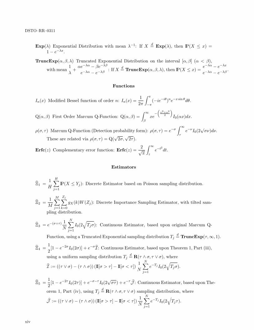
Exp(λ) Exponential Distribution with mean λ−1: If X d= Exp(λ), then IP(X ≤ x) =1 − e−λx.

TruncExp(α, β, λ) Truncated Exponential Distribution on the interval [α, β] (α < β),

with mean1λ

+αe−λα − βe−λβ

e−λα − e−λβ: IfX d= TruncExp(α, β, λ), then IP(X ≤ x) =

e−λα − e−λx

e−λα − e−λβ.

Functions

In(x) Modified Bessel function of order n: In(x) =12π

∫ π

−π(−ie−iθ)ne−x sin θdθ.

Q(α, β) First Order Marcum Q-Function: Q(α, β) =∫ ∞

βxe

−(

x2+α2

2

)I0(αx)dx.

ρ(σ, τ) Marcum Q-Function (Detection probability form): ρ(σ, τ) = e−σ∫ ∞

τe−νI0(2

√σν)dν.

These are related via ρ(σ, τ) = Q(√

2σ,√

2τ).

Erfc(z) Complementary error function: Erfc(z) =2√π

∫ ∞

ze−t2dt.

Estimators

Ξ1 =1H

H∑

j=1

IP(X ≤ Yj): Discrete Estimator based on Poisson sampling distribution.

Ξ2 =1M

M∑

j=1

Zj∑

k=0

gX(k)W (Zj): Discrete Importance Sampling Estimator, with tilted sam-

pling distribution.

Ξ3 = e−(σ+τ) 1N

N∑

j=1

I0(2√Tjσ): Continuous Estimator, based upon original Marcum Q-

Function, using a Truncated Exponential sampling distribution Tjd= TruncExp(τ,∞, 1).

Ξ4 =12[1 − e−2σI0(2σ)] + e−σI: Continuous Estimator, based upon Theorem 1, Part (iii),

using a uniform sampling distribution Tjd= R(τ ∧ σ, τ ∨ σ), where

I := ((τ ∨ σ) − (τ ∧ σ)) (II[σ > τ ] − II[σ < τ ])1N

N∑

j=1

e−TjI0(2√Tjσ).

Ξ5 =12[1 − e−2τI0(2τ)] + e−σ−τ I0(2

√στ) + e−τ J : Continuous Estimator, based upon The-

orem 1, Part (iv), using Tjd= R(τ ∧ σ, τ ∨ σ) sampling distribution, where

J := ((τ ∨ σ) − (τ ∧ σ)) (II[σ > τ ] − II[σ < τ ])1N

N∑

j=1

e−TjI0(2√Tjτ).

xiv

DSTO–RR–0311

Ξ6 =12[1 − e−2σI0(2σ)] + e−σK: Continuous Estimator, based upon Theorem 1, Part (iii),

using sampling distribution Tjd= TruncExp(τ ∧ σ, τ ∨ σ, 1), where

K := (e−(τ∧σ) − e−(τ∨σ)) (II[σ > τ ] − II[σ < τ ])1N

N∑

j=1

I0(2√Tjσ).

Ξ7 =12[1 − e−2τI0(2τ)] + e−σ−τ I0(2

√στ) + e−τ L: Continuous Estimator, based upon The-

orem 1, Part (iv), using sampling distribution Tjd= TruncExp(τ ∧σ, τ ∨σ, 1), where

L := (e−(τ∧σ) − e−(τ∨σ)) (II[σ > τ ] − II[σ < τ ])1N

N∑

j=1

I0(2√Tjτ).

xv

DSTO–RR–0311

xvi

DSTO–RR–0311

1 The Marcum Q-Function

The Marcum Q-Function [Marcum 1950, Marcum 1960, Marcum and Swerling 1960] hashad a long association with the study of target detection by pulsed radars. In radar signalprocessing, the Generalised Marcum Q-Function is the detection probability of a numberof incoherently integrated received signals, in a Gaussian clutter and noise environment[Helstrom 1968, Nuttall 1975 and Shnidman 1989]. It is also an important function inthe study of digital communications. In the latter, it occurs in performance analysisrelated to partially coherent, differentiably coherent and noncoherent communications[Simon 1998 and Simon and Alouini 2003]. The Marcum Q-Function is a definite integraldefined on a semi-infinite domain, whose integrand involves a modified Bessel function,and consequently no closed analytic result is available. Consequently, much research hasbeen devoted to finding good approximations for it. Techniques employed to this endinclude numerical integration schemes and approximations based on the modified Besselfunction in the integrand. Recently, some new expressions for the Marcum Q-Functionhave been derived, linking it to probabilities associated with independent Poisson randomvariables [Weinberg 2005]. These new representations are in a form that is readily adaptedto Monte Carlo integration. Thus the purpose of this work is to investigate the applicationof the stochastic representations in [Weinberg 2005] to the Monte Carlo estimation of theMarcum Q-Function. In particular, we will be restricting attention to what is known asthe standard Marcum Q-Function. The generalised Marcum Q-Function is considered indetail in [Weinberg 2005].

1.1 The Standard Marcum Q-Function

The first order, or standard, Marcum Q-Function is defined by the integral

Q(α, β) :=∫ ∞

βxe

−(

x2+α2

2

)I0(αx)dx, (1)

where I0(·) is the modified Bessel function, of the first kind, of order zero [Bowman 1958and Tsypkin and Tsypkin 1988]. The integrand in (1) is the probability density functionof a Rician distribution [Levanon 1988]. As pointed out in [Sarkies 1976], the latter is thedistribution for the output of a linear law envelope detector with input signal of amplitudeα and narrow band additive Gaussian noise with variance 1.

An equivalent form, which is slightly more natural for radar detection theory, can beobtained by letting α =

√2σ and β =

√2τ . Under this transformation, we define the

alternative form of (1):

ρ(σ, τ) := e−σ∫ ∞

τe−νI0(2

√σν)dν. (2)

In this form, σ is the constant received signal to noise ratio and τ is the normaliseddetection threshold [see Levanon 1988]. Throughout we will refer to (2) as the MarcumQ-Function, and restrict attention to this form, noting that results can easily be extendedto (1) by using the fact that Q(α, β) = ρ(α2

2 ,β2

2 ).

1

DSTO–RR–0311

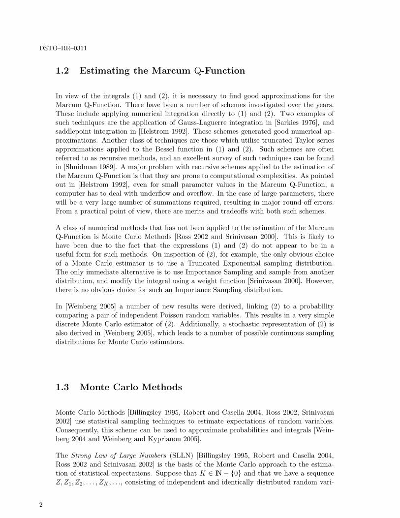
1.2 Estimating the Marcum Q-Function

In view of the integrals (1) and (2), it is necessary to find good approximations for theMarcum Q-Function. There have been a number of schemes investigated over the years.These include applying numerical integration directly to (1) and (2). Two examples ofsuch techniques are the application of Gauss-Laguerre integration in [Sarkies 1976], andsaddlepoint integration in [Helstrom 1992]. These schemes generated good numerical ap-proximations. Another class of techniques are those which utilise truncated Taylor seriesapproximations applied to the Bessel function in (1) and (2). Such schemes are oftenreferred to as recursive methods, and an excellent survey of such techniques can be foundin [Shnidman 1989]. A major problem with recursive schemes applied to the estimation ofthe Marcum Q-Function is that they are prone to computational complexities. As pointedout in [Helstrom 1992], even for small parameter values in the Marcum Q-Function, acomputer has to deal with underflow and overflow. In the case of large parameters, therewill be a very large number of summations required, resulting in major round-off errors.From a practical point of view, there are merits and tradeoffs with both such schemes.

A class of numerical methods that has not been applied to the estimation of the MarcumQ-Function is Monte Carlo Methods [Ross 2002 and Srinivasan 2000]. This is likely tohave been due to the fact that the expressions (1) and (2) do not appear to be in auseful form for such methods. On inspection of (2), for example, the only obvious choiceof a Monte Carlo estimator is to use a Truncated Exponential sampling distribution.The only immediate alternative is to use Importance Sampling and sample from anotherdistribution, and modify the integral using a weight function [Srinivasan 2000]. However,there is no obvious choice for such an Importance Sampling distribution.

In [Weinberg 2005] a number of new results were derived, linking (2) to a probabilitycomparing a pair of independent Poisson random variables. This results in a very simplediscrete Monte Carlo estimator of (2). Additionally, a stochastic representation of (2) isalso derived in [Weinberg 2005], which leads to a number of possible continuous samplingdistributions for Monte Carlo estimators.

1.3 Monte Carlo Methods

Monte Carlo Methods [Billingsley 1995, Robert and Casella 2004, Ross 2002, Srinivasan2002] use statistical sampling techniques to estimate expectations of random variables.Consequently, this scheme can be used to approximate probabilities and integrals [Wein-berg 2004 and Weinberg and Kyprianou 2005].

The Strong Law of Large Numbers (SLLN) [Billingsley 1995, Robert and Casella 2004,Ross 2002 and Srinivasan 2002] is the basis of the Monte Carlo approach to the estima-tion of statistical expectations. Suppose that K ∈ IN − 0 and that we have a sequenceZ,Z1, Z2, . . . , ZK , . . ., consisting of independent and identically distributed random vari-

2

DSTO–RR–0311

ables with mean IE[Z]. Then the simplest form of the SLLN states that

limK→∞

K∑

j=1

Zj

K= IE[Z], (3)

except on a set of probability zero. Hence, the mean of a finite number of the randomvariables gives an approximation to the expectation IE[Z]. As K increases without bound,the approximation becomes more accurate. Thus, in order to estimate the mean IE[Z],we generate a series of independent realisations of Z, and average them. The generationof realisations of random variables, both continuous and discrete, is described in detail in[Ross 2002].

We can apply (3) to a function of the sequence of original random variables. Specifically,if h is an integrable function, whose domain is the sample space of these random variables,then (3) implies that

limK→∞

K∑

j=1

h(Zj)

K= IE[h(Z)]. (4)

Consequently the sumK∑

j=1

h(Zj)K

in (4) can be used to approximate the expectation

IE[h(Z)]. The approximations induced by (3) and (4) utilise statistical sampling to es-timate an expectation, and thus have been referred to as Monte Carlo Methods [Robertand Casella 2004, Ross 2002 and Srinivasan 2002]. Although the SLLN guarantees theconvergence of the sample mean in (3), there are a number of issues with estimators basedupon this principle. The main difficulty is that the sample size K in (3) may have tobe extremely large in order to achieve a prescribed variance. Sometimes it is possible toreduce the required sample size K by sampling from a different distribution, and modify-ing the underlying estimator to make it unbiased. Such techniques, often referred to asvariance reduction techniques, are known as Importance Sampling [Srinivasan 2002].

1.4 Contributions of this Report

This report introduces the idea of applying Monte Carlo simulation schemes to the eval-uation of (2). In particular, we introduce two Monte Carlo estimators of the MarcumQ-Function based upon discrete sampling distributions. One of these is based upon a Pois-son association derived in [Weinberg 2005], while the second is an Importance Samplingestimator. Additionally, we investigate five Monte Carlo estimators, which use continuoussampling distributions. The first of these is based on direct sampling applied to (2), anduses a Truncated Exponential distribution referred to previously. The remaining four arebased upon stochastic representations of the Marcum Q-Function. Two are the result of

3

DSTO–RR–0311

the expressions in [Weinberg 2005], while the second pair arise from a new stochastic formof (2), derived in this report.

The seven Monte Carlo estimators are compared to results derived from adaptive Simpsonquadrature [Lyness and Kaganove 1976]. We also compare some of the estimators toresults based upon partial sum series approximations of Taylor series representations ofthe Marcum Q-Function [Shnidman 1989]. We also examine the simulation gain of pairsof estimators, in an attempt to identify an optimal Monte Carlo estimator of (2).

4

DSTO–RR–0311

2 Representations of the Marcum Q-Function

The key to Monte Carlo estimation of the Marcum Q-Function is to express it in a form thatsuggests a suitable sampling distribution. To this end, we present a number of results,derived in [Weinberg 2005], which readily suggest suitable sampling distributions. Inaddition, a new representation of the Marcum Q-Function is derived, which also suggestsa number of possible Monte Carlo estimators. These expressions will be referred to asprobabilistic-based representations of the Marcum Q-Function.

2.1 A General Result: Theorem 1

In [Weinberg 2005] a number of probabilistic or stochastic representations of the MarcumQ-Function are derived. These express (2) in terms of functions of probabilities of randomvariables. The following Theorem states these results, together with an entirely new result:

Theorem 1 Suppose P = X (ν), ν ∈ IR+ is a series of independent Poisson randomvariables with mean ν. Then the following are equivalent:

(i) ρ(σ, τ) is the Marcum Q-Function (2);

(ii) ρ(σ, τ) = IP[X(τ) ≤ X(σ)];

(iii) ρ(σ, τ) = 12 [1 − e−2σI0(2σ)] + e−σ

∫ σ

τe−νI0(2

√νσ)dν;

(iv) ρ(σ, τ) = 12 [1 − e−2τI0(2τ)] + e−σ−τ I0(2

√στ) + e−τ

∫ σ

τe−νI0(2

√ντ)dν.

The proof that (ii) and (iii) are eqivalent to the Marcum Q-Function can be found in[Weinberg 2005]. Expression (ii) shows that (2) is the same as a comparison of twoPoisson random variables, one with mean being the signal to noise ratio σ, while thesecond has as mean the threshold τ . This gives a very intuitive interpretation to theMarcum Q-Function, which can be found in [Weinberg 2005]. Result (iv) is an entirelynew representation of (2), and was derived using the symmetry relationship of the MarcumQ-Function [see Schwartz, Bennett and Stein 1996].

To prove Theorem 1, we need only derive (iv). We require the two following technicalLemmas:

Lemma 1 For the Marcum Q-Function ρ(·, ·),

ρ(σ, σ) =12[1 − e−2σI0(2σ)]. (5)

5

DSTO–RR–0311

The proof of Lemma 1 can be found in Appendix A of [Weinberg 2005]. Note ρ(σ, σ) isthe detection probability corresponding to the case when the threshold and signal to noiseratio are equal.

The next Lemma is the well-known symmetry relation of the Marcum Q-Function:

Lemma 2 The Marcum Q-Function ρ(·, ·) has the property that

ρ(σ, τ) + ρ(τ, σ) = 1 + e−σ−τ I0(2√στ). (6)

Proof : Although this is a well-known result, and can be found in [Schwartz, Bennett andStein 1996], we present a new probabilistic proof. Assume that X1,X2,X3,X4 ∈ P suchthat X1

d= X4 and X2d= X3. Then Theorem 1 Part (ii) implies

ρ(τ, σ) = IP[X1(σ) ≤ X2(τ)] (7)

andρ(σ, τ) = IP[X3(τ) ≤ X4(σ)]. (8)

Hence it follows that

ρ(σ, τ) + ρ(τ, σ) = IP[X3(τ) = X4(σ)] + IP[X3(τ) < X4(σ)]

+IP[X1(σ) = X2(τ)] + IP[X1(σ) < X2(τ)]. (9)

By construction it follows that

IP[X1(σ) = X2(τ)] = IP[X3(τ) = X4(σ)]. (10)

Thus, by applying (10) to (9), we deduce

ρ(σ, τ) + ρ(τ, σ) = 2IP[X(σ) = X(τ)] + IP[X(τ) < X(σ)]

+ IP[X(σ) < X(τ)]

= 2IP[X(σ) = X(τ)] + IP[X(τ) 6= X(σ)]

= 1 + IP[X(σ) = X(τ)]. (11)

The difference of two independent Poisson distributions is known as a Skellam distribution[Skellam 1946], and it can be shown that the zero probability of such a distribution impliesthat

IP[X(σ) = X(τ)] =∞∑

k=0

e−σ−τ (στ)k

k!2. (12)

6

DSTO–RR–0311

Also, the modified Bessel function of order zero has Taylor series expansion

I0(z) =∞∑

k=0

( z2

4 )k

k!2(13)

[Bowman 1958].

Hence, with the choice of z = 2√στ , we have

IP[X(σ) = X(τ)] = e−σ−τ I0(2√στ ). (14)

Consequently, by an application of (14) to (11), we deduce that

ρ(σ, τ) + ρ(τ, σ) = 1 + e−σ−τ I0(2√στ), (15)

which completes the proof of the Lemma.

2

We are now in a position to prove Part (iv) of Theorem 1.

Proof of Theorem 1, Part (iv):

By interchanging σ and τ in Part (iii) in Theorem 1, we note that

ρ(τ, σ) = ρ(τ, τ) +∫ τ

σIP[X(ν) = X(τ)]dν. (16)

An application of (16) to the symmetry relation in Lemma 2, and applying Lemma 1, wededuce that

ρ(σ, τ) = 1 + e−σ−τ I0(2√στ) − ρ(τ, τ) −

∫ τ

σIP[X(ν) = X(τ)]dν

= 1 + e−σ−τ I0(2√στ) − 1

2[1 + e−2τI0(2τ)]

+∫ σ

τIP[X(ν) = X(τ)]dν

=12

+ e−σ−τ I0(2√στ) − 1

2[1 + e−2τ I0(2τ)]

+∫ σ

τIP[X(ν) = X(τ)]dν

=12[1 − e−2τ I0(2τ)] + e−σ−τ I0(2

√στ) +

∫ σ

τIP[X(ν) = X(τ)]dν. (17)

7

DSTO–RR–0311

The proof is completed by recalling that IP[X(ν) = X(τ)] = e−ν−τI0(2√ντ), and applying

this to (17).

2

In the next Section we derive a number of estimators, based upon the results of Theorem1.

8

DSTO–RR–0311

3 Monte Carlo Estimators of the Marcum

Q-Function

We are now in a position to introduce a series of Monte Carlo sampling estimators of theMarcum Q-Function (2). Estimators based upon sampling from both discrete and contin-uous distributions will be considered. At this stage we limit our attention to introducingthese estimators. For reference, Appendix A contains some details on the calculationof variances of random variables. Additionally, Appendix B outlines how realisations ofrandom variables, from a prescribed distribution, can be obtained.

3.1 Discrete Estimators

To begin, we consider a number of estimators of the Marcum Q-Function using discretesampling distributions. Firstly, we illustrate how the Monte Carlo scheme works in thiscase. With reference to (4), we suppose Z is a discrete random variable with supportIN = 0, 1, 2, . . ., and h is a function with the same support. We want to estimate theexpectation IE[h(Z)]. A basic Monte Carlo estimator of this expectation can be based on

IE[h(Z)] =∞∑

k=0

h(k)IP[Z = k] ≈ 1K

K∑

j=1

h(Zj), (18)

where the sequence Z1, Z2, . . . , ZK consists of independent and identically distributedcopies of the random variable Z. Throughout we will employ the statistical convention ofdenoting an estimator by using a hat over its symbol. Hence, we write ℵ to represent theestimator in (18), so that

ℵ =1K

K∑

j=1

h(Zj). (19)

3.1.1 A Standard Monte Carlo Estimator

The first Monte Carlo estimator we consider is based directly on Theorem 1, Part (ii). Thisresult shows that the Marcum Q-Function (2) can be represented as a probability of theform IP(X ≤ Y ), whereX and Y are independent (Poisson) random variables with supportIN. With reference to (18), we choose a two-dimensional version of h: h(x, y) = II[x ≤ y],where II is the indicator function. This means that h(x, y) = 1 if x ≤ y and is zerootherwise. We also let ψ(X,Y ) = IEh(X,Y ) ≡ IP[X ≤ Y ], which is the probability underinvestigation.

Then the standard Monte Carlo estimator of ψ(X,Y ) is

Ξ =1K

K∑

j=1

h(Xj , Yj)

9

DSTO–RR–0311

=1K

K∑

j=1

Yj∑

k=0

II[Xj = k], (20)

where the pairs (Xj , Yj) consist of independent and identically distributed copies of (X,Y ).The generation of realisations of Poisson random variables is described in [Ross 2002], andalso in Appendix B, to which the reader is referred.

It is not difficult to show that (20) is an unbiased estimator of ψ(X,Y ), meaning thatIE[Ξ] = ψ(X,Y ), so that the estimator is centred on the probability it is estimating. Itsvariance can be shown to be

VV[Ξ] =1K

[ψ(X,Y ) − ψ(X,Y )2

]. (21)

The expression in (21) shows that as the sample size increases without bound, the esti-mator’s variation from its expected value decreases to zero. The issue of interest is howlarge must N be so that this variance is within a prescribed tolerance. Suppose we requireVV(P ) ≤ ε, for some ε > 0. Using (21), it is not difficult to see that we need to choose

K =

⌊ψ(X,Y ) − ψ(X,Y )2

ε

⌋+ 1, (22)

where bxc is the greatest integer not exceeding x. Thus, K is of order 1ε , unless the

probability ψ(X,Y ) is very small relative to ε. Equation (22) shows the inherent problemsone faces with Monte Carlo estimation. The SLLN guarantees that the estimator willconverge, but the tradeoff is that this might be at the expense of a very large numberof simulation runs. There is an exception to this. In view of the variance (21), if theprobability ψ(X,Y ) is very small, then the variance will also be very small, independentlyof the number of simulation runs K. The probability ψ(X,Y ) will be very small whenthe random variable X is significantly larger than Y . This case implies Monte Carlomethods will have the best performance for the estimation of probabilities of rare events.Nevertheless, we will show that an alternative to (20) can be produced, which is a globallymore efficient estimator.

3.1.2 A Poisson-Based Sampling Estimator: Ξ1

The following approach is motivated by the work of [Srinivasan 2000] on the so-calledG-function estimator, and also by the analysis of [Bucklew 2003] on bias point selection.

Note that, since we are assuming X and Y are independent, we can write

IP[X ≤ Y ] =∞∑

k=0

IP[X ≤ k]IP[Y = k], (23)

and so, in view of (18), a Monte Carlo estimator of (23) is

Ξ1 =1H

H∑

j=1

IP[X ≤ Yj]

10

DSTO–RR–0311

=1H

H∑

j=1

Yj∑

k=0

gX(k), (24)

where each Yj is an independent realisation of Y , and we define gX(k) = IP[X = k]. Hence,we can estimate probabilities of the form IP[X ≤ Y ] by generating independent realisationsof Y and averaging the cumulative distribution function over these values. Expression (23)provides a means of compression of the probability of interest, analogous to that used in[Srinivasan 2000]. Sampling from a Poisson distribution, as remarked previously, can beeasily achieved through any of the algorithms given in [Ross 2002] and Appendix B.

We now examine the estimator (24) more closely. Firstly, it is not difficult to show thatit is also an unbiased estimator of ψ(X,Y ). To see this, observe that

IE[Ξ1] =∞∑

m=0

IP[Y = m]m∑

k=0

gX(k)

=∞∑

m=0

IP[Y = m]IP[X ≤ m]

= IP[X ≤ Y ].

Secondly, it is not difficult to show its variance is given by

VV[Ξ1] =1H

IE

[Y∑

k=0

gX(k)

]2

− ψ(X,Y )2 . (25)

Observe that the sum in the first expectation in (25) is a (random) sum of probabilities ofthe same random variable X, and so is bounded by one. This implies that (25) is smallerthan (21), for the same number of simulations (K = H), and consequently estimator (24)is more efficient than (20). Hence we will not consider the standard Monte Carlo estimator(20) any further.

The simulation gain, of a pair of estimators, is a quantitative measure of the improvementone Monte Carlo estimator has over another, in terms of reducing the number of simula-tions. For the same level of variance, we are interested in the size of the ratio of K andH. By equating the expressions (21) and (25), we obtain

Γ =K

H=

ψ(X,Y ) − ψ(X,Y )2

IE

[Y∑

k=0

gX(k)

]2

− ψ(X,Y )2, (26)

and the previous remarks imply that Γ > 1. Consequently, for the same level of variance,the estimator (24) requires less simulation runs than (20). To determine the exact levelof improvement is a somewhat complicated exercise. This is due to the fact that boththe variances (21) and (25) depend on the unknown probability ψ(X,Y ), as does thegain (26). Secondly, the variance (25), and so (26), both depend on the expectation

11

DSTO–RR–0311

IE[∑Y

k=0 gX(k)]2

, which is not readily evaluated. Both these difficulties can be partiallyresolved using estimation. This will at least give a partial understanding of the potentialimprovement provided by the estimator (24).

3.1.3 An Importance Sampling Estimator: Ξ2

It is now worth considering whether an Importance Sampling estimator can provide animprovement on the estimator (24). Importance Sampling (IS) [Robert and Casella 2004,Ross 2002 and Srinivasan 2002] has been developed in an attempt to address the sample sizeissues associated with Monte Carlo methods. This is a variance reduction technique, whichattempts to reduce the Monte Carlo estimator’s variance by sampling from a distributionnot directly suggested by the probability being estimated. In the current context, onewould introduce biasing distributions, which would be used in (20) instead of Xj and Yj .In order to make the resulting estimator unbiased, it is weighted at each point by a weightfunction. As pointed out in [Srinivasan 2002], these biasing distributions are chosen in anattempt to increase the distribution of points relevant to the estimation, or in other words,sample points that are important to the Monte Carlo simulation. A consequence of thesuccessful achievement of this is that the resulting estimator’s variance should be reduced.This will also result in a reduction in simulation runs, when compared to a standard MonteCarlo estimator.

Much work has been devoted to the design of efficient IS biasing distributions [Srinivasan2002]. However, it is important to remember that Monte Carlo IS techniques tend towork best when estimating probabilities associated with rare events, such as false alarmprobabilities in CFAR processes [see Ross 2002 and Srinivasan 2002]. In the currentcontext, we are interested in the Marcum Q-Function (2), which take values in a fullspectrum of possibilities. Hence it is possible that Importance Sampling will not improvesignificantly the performance of Monte Carlo estimators of the Marcum Q-Function.

We attempt the construction of an Importance Sampling estimator based on (24). Thekey to this is to replace the random variables Yj, j ∈ 1, 2, . . . ,H with a new biasingdistribution Zj, for j in the same indexing set, and weighting the estimator (24) at eachpoint, to make the resulting estimator unbiased. Such an estimator can be defined as

Ξ2 =1M

M∑

j=1

Zj∑

k=0

gX(k)W (Zj), (27)

where the random variables Zj are independent and identically distributed copies of thebiasing random variable Z. The function W (·) in (27) is a weight function, which is chosento make the estimator unbiased for ψ(X,Y ). It can be shown that the latter necessitatesthe choice of

W (k) =IP[Y = k]IP[Z = k]

, (28)

which also shows that we must ensure that any choice made for the biasing distributiondoes not have zero probabilities on its support. This automatically excludes the choice ofa truncated Poisson distribution, which would have been a somewhat natural choice. The

12

DSTO–RR–0311

latter is the case because a Poisson distribution is centered on its mean, and its varianceis also equal to its mean. Thus a truncated Poisson could be constructed that gives morelikelihood near its mean value.

The variance of (27) can be shown to be

VV[Ξ2] =1M

IE

[Z∑

k=0

gX(k)W (Z)

]2

− ψ(X,Y )2

(29)

=1M

IE

(

Y∑

k=0

gX(k)

)2

W (Y )

− ψ(X,Y )2

,

where the latter equality follows by applying the definition of the weight function (28),and expanding out the expectation. Comparing (29) to (25), we see that if a biasing dis-tribution can be chosen so that the weight function never exceeds unity, the correspondingImportance Sampling estimator will be more efficient. In the context of interest, since thebiasing distribution will have the same support as Y , namely the nonnegative integers, thisproperty will not hold [see Srinivasan, 2002]. There are a number of Importance Samplingbiasing distributions that have been studied in the literature. These have been developedby using properties of the unique optimal biasing distribution associated with ImportanceSampling techniques [Srinivasan, 2002]. To illustrate this in our current situation, considerthe choice of biasing distribution with point probabilities

IP[Z = m] = ψ(X,Y )−1IP[Y = m]m∑

k=0

gX(k). (30)

Applying (30) to the variance (29), we see that the corresponding estimator (27) has zerovariance. The distribution (30) cannot be used in practice, because it depends on theunknown probability of interest, namely ψ(X,Y ). However, as pointed out in [Srinivasan2002], its form suggests how potential biasing distributions can be constructed. Specifi-cally, it suggests a biasing distribution should be proportional to the original distribution,and concentrated on the event or region of interest. Based on such observations, potentialbiasing distributions include scaling and translation applied to the original distribution[Srinivasan 2002], exponential twisting or tilting [Ross 2002 and Srinivasan 2002] andChernoff Importance Sampling distributions [Gerlach 1999].

We consider the case of a discrete tilted biasing distribution [Ross 2002]. Such a distribu-tion has point probabilities given by

IP[Z = k] = IP[Z = k|θ] =θkIP[Y = k]

∞∑

m=0

θmIP[Y = m], (31)

for all k ∈ IN, where θ > 0 is a biasing parameter. Observe that the normalising constanton the denominator of (31) is the probability generating function of Y [see Billingsley 1995and Durrett 1996]. We assume that Y is Poisson with parameter λ. Consequently, it can

13

DSTO–RR–0311

be shown that∑∞

m=0 θmIP[Y = m] = e−λ(1−θ), and hence (31) becomes

IP[Z = k] =e−λθ(λθ)k

k!, (32)

which implies that the biasing distribution is also Poisson, but with a parameter of λθ.Additionally, it follows that the weight function (28) is W (k) = θ−ke−λ(1−θ). This weightfunction implies the variance (29) becomes

VV[Ξ2] =1M

e−λ(1−θ)IE

θ−Y

(Y∑

k=0

gX(k)

)2− ψ(X,Y )2

. (33)

An issue with the variance (33) is that if θ < 1, the term θ−Y in the expectation componentof (33) will have the potential to grow exponentially. This is due to the fact that Y takesvalues in the nonnegative integers. Also, with the choice of θ > 1, the term e−λ(1−θ) willalso grow exponentially, but not in such a dynamic way. In this case, the term θ−Y willcause the expectation in (33) to decrease exponentially, and has the potential to controlthe behaviour of the multiplier term. Hence we restrict attention to the case where θ ≥ 1.Our interest is whether a θ > 1 can be found, such that the variance (33) is smaller than(25), when H = M . As before, we let the simulation gain be Γ = H

M . Then for the samevariance in (25) and (33),

Γ =

IE

[Y∑

k=0

gX(k)

]2

− ψ(X,Y )2

e−λ(1−θ)IE

θ−Y

(Y∑

k=0

gX(k)

)2− ψ(X,Y )2

. (34)

In contrast to the gain (26), it is not mathematically straightforward to determine whetherthe gain (34) exceeds 1, for particular choices of θ. For specific choices of the free para-meters one can investigate this gain numerically. Also, it is possible to attempt to choosea θ that minimises the variance (33), by employing a stochastic Newton recursion, as in[Srinivasan 2000]. The disadvantage of the latter is that it necessitates the introductionof two additional Monte Carlo estimators, as well as a recursion scheme, which can addconsiderably to the numerical computation times. We will examine these gains further inSection 4.

3.2 Continuous Estimators

Estimators based upon continuous sampling distributions are now considered. On inspec-tion of the Marcum Q-Function integral (2), continuous sampling distributions are themost obvious approach. In such cases, we are again interested in estimating the expecta-tion IE[h(Z)], but we assume that Z has a density g on a subset of the real line, Ω ⊂ IR.Then, in view of (4), this implies

IE[h(Z)] =∫

Ωh(z)g(z)dz ≈ 1

K

K∑

j=1

h(Zj), (35)

14

DSTO–RR–0311

where each Zj is generated from a random variable with density g. The Marcum Q-Function integral (2) has an exponential term in its integrand, which can be weighted toproduce a density that can then be used to construct a sampling distribution. We willconsider this estimator, as well as a number of others that can be derived from Theorem1.

3.2.1 Estimator Based on Original Marcum Q-Function Integral: Ξ3

As remarked previously, an obvious choice for biasing distribution of (2) is a TruncatedExponential distribution, with this distribution the restriction of the standard exponentialdistribution to the interval [τ,∞). We denote this distribution by TruncExp(τ,∞, 1), andits corresponding density is fT (ν) = eτ−ν , for ν ≥ τ . By scaling the Marcum Q-Functionintegral (2) by e−τ , we arrive at the estimator

Ξ3 = e−(σ+τ) 1N

N∑

j=1

I0(2√Tjσ), (36)

where each Tj is generated by independently sampling from the TruncExp(τ,∞, 1) dis-tribution. Sampling from the latter is relatively straightforward, since it only requiresone to sample from a uniform distribution on the unit interval [0,1], and then apply asimple transformation. Specifically, since the cumulative distribution function of T d=TruncExp(τ,∞, 1) is FT (ν) = 1 − eτ−ν , for ν ≥ τ , and its inverse is F−1

T (ν) = τ −log(1 − ν), it follows from Appendix B that T can be simulated using τ − log(R), whereR

d= R[0, 1].

It is not difficult to show this is also an unbiased estimator of (2). Observe that

IE[Ξ3] = e−(σ+τ)IE[I0(2√Tσ)]

= e−(σ+τ)∫ ∞

τeτ−νI0(2

√νσ)dν

=∫ ∞

τe−σ−νI0(2

√νσ)dν,

which is (2), implying Ξ3 is unbiased.

The variance of estimator Ξ3 is given by the expression

VV[Ξ3] = e−2(σ+τ) 1N

VV[I0(2√Tσ)]

= e−2(σ+τ) 1N

[IE[I2

0 (2√Tσ)] −

(IE[I0(2

√Tσ)]

)2]. (37)

Using the definition of T , it follows that

IE[I20 (2

√Tσ)] =

∫ ∞

τeτ−νI2

0 (2√νσ)dν, (38)

15

DSTO–RR–0311

and alsoIE[I0(2

√Tσ)] =

∫ ∞

τeτ−νI0(2

√νσ)dν, (39)

so that numerical integration techniques can be applied to both (38) and (39), which thenyield a numerical estimate of (37). We will consider continuous estimator’s variances inmore detail in Section 4.

3.2.2 An Estimator Based on Theorem 1 Part (iii), with Uniform Sam-

pling Distribution: Ξ4

We now consider estimators of the Marcum Q-Function, based upon the results of Theorem1, Parts (iii) and (iv), that use continuous sampling distributions. The first of these isbased upon a uniform samping distribution applied to Part (iii) of Theorem 1.

Let T be a uniformly distributed random variable on the interval [τ ∧ σ, τ ∨ σ], so thatT

d= R(τ ∧ σ, τ ∨ σ). Such a random variable has density fT (ν) = 1(τ∧σ)−(τ∨σ) , for τ ∧ σ <

ν < τ ∨ σ. Since this density is independent of its free variable ν, we can insert it intothe expression in Part (iii) of Theorem 1, and multiply the integral by its reciprocal tobalance the equation. In view of this, we focus on the integral component of Part (iii) inTheorem 1.

Observe that

I :=∫ σ

τe−νI0(2

√νσ)dν (40)

≡∫ τ∨σ

τ∧σe−νI0(2

√νσ)dν × (II[σ > τ ] − II[σ < τ ])

= [(τ ∨ σ) − (τ ∧ σ)]∫ τ∨σ

τ∧σfR(ν)e−νI0(2

√νσ)dν

× (II[σ > τ ] − II[σ < τ ]) . (41)

Consequently, (41) is in a suitable form to apply the SLLN (4) to produce a Monte Carloestimator. Specifically, if we let Tj

d= R(τ ∧ σ, τ ∨ σ) be a series of independent andidentically distributed uniform random variables, then we can derive estimates of theMarcum Q-Function from

Ξ4 =12[1 − e−2σI0(2σ)] + e−σI, (42)

where I is estimated from

I = ((τ ∨ σ) − (τ ∧ σ)) (II[σ > τ ] − II[σ < τ ])1N

N∑

j=1

e−TjI0(2√Tjσ). (43)

It is relatively straightforward to show that (42) is an unbiased estimator of the MarcumQ-Function ρ(σ, τ). Its variance, however, is more involved. Note that the deterministic

16

DSTO–RR–0311

components in (42) contribute nothing to the estimator’s variance. Also, note that thesquare of the difference of the indicator functions in (43) will be unity. Hence it followsthat

VV[Ξ4] = e−2σVV[I]

= e−2σ 1N

[(τ ∨ σ) − (τ ∧ σ)]2 VV[e−T I0(2

√Tσ)

]

=e−2σ

N[(τ ∨ σ) − (τ ∧ σ)]2

×(

IE[e−2T I20 (2

√Tσ)] −

(IE[e−T I0(2

√Tσ)]

)2). (44)

We can, as previously, use the definition of T to write the expectations in (44) as integrals,but we do not include these here. The two expression (37) and (44), for the variancesof estimators Ξ3 and Ξ4 respectively, do not provide much insight into the appropriateestimator’s performance per se. Mathematically, it is quite difficult to work out closed formexpressions that lead to useful simulation gain estimates. We will thus produce numericalestimates and plots of simulation gains in Section 4. These expressions for estimator’svariance have been included for completeness.

3.2.3 An Estimator Based upon Theorem 1, Part (iv) using a Uniform

Sampling Distribution: Ξ5

This estimator also uses a uniform sampling distribution, but is instead based upon Part(iv) of Theorem 1. As previously, we let T d= R(τ ∧ σ, τ ∨ σ). The only part that involvesMonte Carlo estimation is the integral component in Part (iv) of Theorem 1. As in thederivation of (41), observe that we can write

J :=∫ σ

τe−νI0(2

√ντ)dν (45)

≡∫ τ∨σ

τ∧σe−νI0(2

√ντ)dν × (II[σ > τ ] − II[σ < τ ]). (46)

Thus, as in the argument to construct the estimator (42), we can use (46) to produce theestimator

Ξ5 =12[1 − e−2τ I0(2τ)] + e−σ−τ I0(2

√στ) + e−τ J , (47)

where the integral (45) is estimated from

J = ((τ ∨ σ) − (τ ∧ σ)) (II[σ > τ ] − II[σ < τ ])1N

N∑

j=1

e−TjI0(2√Tjτ), (48)

17

DSTO–RR–0311

and each Tj is an independent realisation of T . Again, it is relatively straightforward toshow that (47) is an unbiased estimator of the Marcum Q-Function. Also, it is not difficultto write down an expression for its variance. In particular, it can be shown that

VV[Ξ5] =e−2τ

N[(τ ∨ σ) − (τ ∧ σ)]2

×(

IE[e−2T I20 (2

√Tτ)] −

(IE[e−T I0(2

√Tτ)]

)2). (49)

3.2.4 Estimator Based upon Theorem 1, Part (iii) with Truncated Ex-

ponential Sampling Distribution: Ξ6

We now consider using a sampling distribution based upon a truncated exponential family.In this case, we consider Part (iii) of Theorem 1, and in view of the integral (40), weintroduce a Truncated Exponential distribution T

d= TruncExp(τ ∧ σ, τ ∨ σ, 1). Such adistribution has density fT (t) = e−t

e−(τ∧σ)−e−(τ∨σ) , and can be simulated using − log[e−(τ∧σ)−

R[e−(τ∧σ) − e−(τ∨σ)], where R d= R[0, 1].

Let K be the estimator

K = (e−(τ∧σ) − e−(τ∨σ)) (II[σ > τ ] − II[σ < τ ])1N

N∑

j=1

I0(2√Tjσ), (50)

where each Tjd= TruncExp(τ ∧ σ, τ ∨ σ, 1). Then we can define the estimator

Ξ6 =12[1 − e−2σI0(2σ)] + e−σK. (51)

It is again not difficult to show this is an unbiased estimator of (2), with variance givenby

VV[Ξ6] =e−2σ

N

[e−(τ∧σ) − e−(τ∨σ)

]2

×(

IE[I20 (2

√Tσ)] −

(IE[I0(2

√Tσ)]

)2). (52)

3.2.5 An Estimator Based upon Part (iv) of Theorem 1 with Truncated

Exponential Sampling Distribution: Ξ7

The final estimator we consider is also based upon a Truncated Exponential distribution,using Part (iv) of Theorem 1. Let L be the estimator

L = (e−(τ∧σ) − e−(τ∨σ)) (II[σ > τ ] − II[σ < τ ])1N

N∑

j=1

I0(2√Tjτ), (53)

18

DSTO–RR–0311

where each Tjd= TruncExp(τ ∧ σ, τ ∨ σ, 1) are independent random variables. Then we

can defineΞ7 =

12[1 − e−2τ I0(2τ)] + e−σ−τI0(2

√στ ) + e−τ L. (54)

It is also easy to show this is an unbiased estimator of (2), with variance given by

VV[Ξ7] =e−2τ

N

[e−(τ∧σ) − e−(τ∨σ)

]2

×(

IE[I20 (2

√Tτ)] −

(IE[I0(2

√Tτ)]

)2). (55)

19

DSTO–RR–0311

4 Performance and Analysis of Estimators

We now consider the performance of the estimators introduced in Section 3. This willbe done by considering numerical estimates, and comparing them to estimates obtainedby numerical integration. In particular, we will be interested in how these estimatorsperform in comparison to Adaptive Simpson Quadrature (ASQ) [Lyness and Kaganove1976]. Throughout we will use a tolerance of 10−8 for ASQ. Additionally, we will includesome comparisons to results based upon truncated Taylor series approximations [Shnidman1989]. We base the latter on the following Taylor series expansion, which can be found in[Schwartz, Bennett and Stein 1996, Equation A-4-7]:

ρ(σ, τ) = 1 − e−(σ+τ)∞∑

m=1

(√ τ

σ

)mIm(2

√στ). (56)

One can truncate the Taylor series in (56), and use the partial sum as an approximationfor ρ(σ, τ).

Before presenting these numerical comparisons, we firstly consider simulation gains.

4.1 Simulation Gains

Appendix C contains a number of plots of simulation gains. For the sake of brevity, weonly consider a subset of the 21 possible combinations of pairs of 7 estimators. Recallthat the simulation gain Γ measures the number of simulation runs one estimator needsto match the same level of variance as another estimator. Thus it can indicate whetherone estimator will perform as well as another, except for less simulation runs.

To begin, we consider whether the Importance Sampling estimator Ξ2 is an improvementon the standard Poisson estimator Ξ1. Figure C.1 shows a plot of the simulation gain (34),with the IS estimator using θ = 2. The surface shows the logarithmic gain, as a functionof σ and τ . Figure C.2 shows a cross sectional view of it. In view of (34), since the surfaceshows that log(Γ) < 0, we conclude that the estimator Ξ1 will be more efficient. Also,similar such simulation gain plots, for θ increasing in the IS estimator Ξ2, did not indicatethat the IS estimator is more efficient than Ξ1.

Figures C.3 to C.10 provide gain plots, comparing the Poisson estimator Ξ1 to some ofthe estimators based upon continuous sampling distributions and the results of Theorem1, Parts (iii) and (iv). In these plots the gain Γ is the ratio of the number of simulationsused in estimators Ξ4, Ξ5, Ξ6 and Ξ7, compared to the number of simulations needed forthe Poisson Estimator Ξ1. In these cases if Γ is greater than zero on the logarithmic scale,the Poisson Estimator requires less simulation runs.

Figure C.3 compares the estimator Ξ4 to Ξ1, and as the cross-sectional view shows inFigure C.4, there are only small regions where Ξ4 will be more efficient.

Figure C.5 examines the performance of Ξ5 relative to Ξ1, and Figure C.6 shows a cross-

20

DSTO–RR–0311

sectional view. As for the previous case, there are regions where the continuous estimatoroutperforms the Poisson estimator.

Figure C.7, in contrast to the two examples considered previously, showed significant globalimprovements on the estimator Ξ1. This plot is of the gain of estimator Ξ6 relative to Ξ1.Both Figure C.7, and the cross-sectional plot of Figure C.8, show that the estimator Ξ6

will frequently outperform the Poisson estimator.

The final comparison we consider is that of the simulation gain of estimator Ξ7 relativeto Ξ1. As can be observed from Figures C.9 and C.10, there are many choices of σ andτ -parameters which will result in simulation savings in using estimator Ξ7.

The Figures show that for each estimator there are values of σ and τ for which lesssimulation runs are required than for Ξ1.

The main conclusion from these simulation gain plots is that some of the estimators basedupon Theorem 1, Parts (iii) and (iv), will outperform the discrete Poisson estimator,based upon Part (ii) of Theorem 1. Estimators Ξ6 and Ξ7 showed the most promise,while the other continuous estimators considered also had regions where improvementsover the Poisson estimator were possible. Clearly, the Importance Sampling estimator Ξ2

had inferior performance to the Poisson estimator Ξ1.

4.2 Numerical Results

We now consider numerical results of these estimators, and will be more interested inaccuracy when compared to results obtained using ASQ. All estimates can be found inthe Tables in Appendix D. Table D.1 contains some estimates of ρ(σ, τ) based upon atruncated Taylor series approximation using (56). The partial sum uses 100 terms toobtain the estimate. Table D.1 also contains estimates obtained using ASQ, and theabsolute error between the estimates is included. This error is just the difference betweenthe two estimates. These results will be used to compare the performance of the estimatorsof Section 3. We do not consider the IS estimator Ξ2, due to the fact that its simulationgain plot showed it to be generally inferior to the Poisson estimator Ξ1.

Table D.2 contains a selection of estimates for estimator Ξ1. The two free parameters σand τ range from 1 to 5, and the Table shows estimates based on samples using N = 103,104, 105 and 106. Each estimate is compared to one obtained via ASQ, and the absoluteerror is also given. The Table shows that the estimator performs well for larger N , butstill requires a larger sample size to achieve more uniform accuracy.

Table D.3 shows the performance of the standard continuous estimator Ξ3, again withcomparisons to results based on ASQ, and with N varying as in Table D.2. The errorsseem consistently smaller than those obtained in Table D.2, indicating Ξ3 is slighly moreaccurate. Overall, however, there is not a major improvement over Ξ1, just a small orderof magnitude improvement.

21

DSTO–RR–0311

We now consider estimators based upon the stochastic representations of Theorem 1, Parts(iii) and (iv). Tables D.4 and D.5 contain estimates based upon Ξ4 and Ξ6. Both theseestimators are based upon Part (iii) of Theorem 1, with Ξ4 using a uniform samplingdistribution, and Ξ6 employing a Truncated Exponential sampling distribution. Table D.4shows estimates using N = 103 and 104, and compares results again to those obtained viaASQ. It is clear that for the relatively modest sample sizes, these estimators are performingbetter than those considered in Tables D.2 and D.3. The results in Table 5 are generatedfor the same estimators as in Table D.4, but use N = 105 and 106. These show furtherimprovements are made on the accuracy of estimators Ξ4 and Ξ6.

Tables D.6 and D.7 show simulation results using estimators Ξ5 and Ξ7, which are basedupon Theorem 1, Part (iv). Ξ5 uses a uniformly sampled distribution, while Ξ7 is basedupon a Truncated Exponential distribution. Table D.6 contains results for the case whereN = 103 and 104, while Table D.7 contains estimates for N = 105 and 106. These twoTables show that both estimators are performing well, and that Ξ5 is performing extremelywell in some cases.

The final set of estimates can be found in Table D.8, which directly compares the perfor-mance of estimators Ξ4, Ξ5, Ξ6 and Ξ7. Each estimator uses a sample of size N = 106, andeach result is again compared to ASQ. As can be observed, the estimators are performingwell for this number of simulations, with Ξ5 returning the smallest errors on average.

It is interesting to compare the results of Table D.8 with those in Table D.1, the latter beingestimates based upon a partial sum approximation of (56). A sample size of N = 106,for each of the estimators considered in Table D.8, are not as accurate as an estimatebased upon a partial sum of 100 terms. Increasing N in these estimators will improvetheir accuracy, but will increase computation times. It is worth noting, however, that thecomputation time to compute the partial sum series from (56) is faster than computing106 simulation runs in a Monte Carlo estimator. This sample size issue is a significantlimiting factor on the application of Monte Carlo methods.

22

DSTO–RR–0311

5 Conclusions

This report is an investigation of the Monte Carlo estimation of Marcum’s Q-Function.Using some new stochastic representations derived in [Weinberg 2005], together with anew result derived in this report, seven estimators were defined and analysed. Two ofthese estimators were based upon discrete sampling distributions. One was based uponthe Poisson association in Part (ii) of Theorem 1. The second was an importance samplingestimator, using a tilted sampling distribution. It was found that the Poisson estimatorΞ1 was the better of the two estimators. The remaining five estimators used continuoussampling distributions. One was based upon a Truncated Exponential Distribution, onthe semi-infinite domain [τ,∞). The remaining four estimators were based upon Parts (iii)and (iv) of Theorem 1. Two used Uniform sampling distributions, while the remainingpair used Truncated Exponential sampling distributions, on a finite domain. Out of allthe continuous estimators, it was found that they had regions where they performed verywell, and similarly regions where their performance was moderate. It was found that themost efficient of the seven estimators was the one based upon Part (iv) of Theorem 1,using a uniform sampling distribution, referred to as Ξ5.

The performance analysis of the seven estimators indicated that large sample sizes areneeded to obtain accurate results, although some of the estimators returned accurateresults for relatively small sample sizes, such as Ξ5 and Ξ7. Simulation gain considerationsindicated that a number of these estimators may be useful from a practical perspective.

6 Acknowledgements

The authors would like to thank the sponsor, Commander Surveillance & Response Group,RAAF Williamtown, for supporting this research through Task AIR 04/206. The Co-author Louise Panton expresses thanks to DSTO for providing the opportunity to beinvolved in its Summer Vacation Scholarship Program. Thanks are also due to Dr GraemeNash, of Weapons Systems Division, for reviewing the report.

23

DSTO–RR–0311

References

1. Bowman, F. (1958), Introduction to Bessel Functions. (Dover, New York).

2. Billingsley, P. (1995), Probability and Measure. (Wiley, New York).

3. Bucklew, J. A. and Gubner, J. A. (2003), Bias Point Selection in the ImportanceSampling Monte Carlo Simulation of Systems. IEEE Trans. Sig. Proc. 51, 152-159.

4. Durrett, R. (1996), Probability: Theory and Examples. (Wadsworth Publishing Com-pany, California).

5. Gerlach, K. (1999), New Results in Importance Sampling. IEEE Trans. Aero. Elec.Sys. 35, 917-925.

6. Helstrom, C. W. (1968), Statistical Theory of Detection. (Pergamon, New York).

7. Helstrom, C. W. (1992), Computing the Generalized Marcum Q-Function. IEEETrans. Info. Theory, 38, 1422-1428.

8. Levanon, N. (1988), Radar Principles. (John Wiley & Sons, New York).

9. Lyness, J. N. and Kaganove, J. J. (1976), Comments on the Nature of AutomaticQuadrature Routines. ACM Trans. Math. Soft. 2, 65-81.

10. Marcum, J. L. (1960), A statistical theory of target detection by pulsed radar. IRETrans. Info. Theory, IT–6, 59–144.

11. Marcum, J. I. (1950), Table of Q functions. Rand Corp., Santa Monica, CA. U.S.A.F.Project RAND Research Memorandum M–339.

12. Marcum, J. I. and Swerling, P. (1960), Studies of target detection by pulsed radar.IEEE Trans. Info. Theory, IT-6.

13. Nuttall, A. H. (1975), Some integrals involving the QM Function. IEEE Trans. Info.Theory, 21, 95–96.

14. Robert, C. P. and Casella, G. (2004), Monte Carlo Statistical Methods. (Springer,New York).

15. Ross, S. M. (2002), Simulation. (Academic Press, San Diego, California).

16. Sarkies, K. (1976), Computer Program for the Evaluation of the Marcum Q-Function.WRE-Technical Note 1727

17. Schwartz, M., Bennett, W. R. and Stein, S. (1966), Communication Systems andTechniques. (McGraw-Hill, New York).

18. Shnidman, D. A. (1989), The Calculation of the Probability of Detection and theGeneralised Marcum Q-Function. IEEE Trans. Info. Theory, 35, 389–400.

19. Simon, M. K. (1998), A New Twist on the Marcum Q-Function and its Application.IEEE Comms. Lett., 2, 39–41.

24

DSTO–RR–0311

20. Simon, M. K. and Alouini, M.-S. (2003), Some New Results for Integrals Involving theGeneralised Marcum Q Function and Their Application to Performance EvaluationOver Fading Channels. IEEE Trans. Wireless Comms., 2, 611–615.

21. Skellam, J. G. (1946), The frequency distribution of the difference between two Poissonvariates belonging to different populations. J. Royal Statist. Soc. A, 109, 296.

22. Srinivasan, R. (2000), Simulation of CFAR detection algorithms for arbitrary clutterdistributions. IEE Proc. Radar, Sonar Navig. 147, 31-40.

23. Srinivasan, R. (2002), Importance Sampling: Applications in Communications andDetection. (Springer-Verlag, Heidelberg).

24. Tsypkin, A. G. and Tsypkin, G. G. (1988), Mathematical Formulas: Algebra, Geom-etry and Mathematical Analysis. (Mir Publishers, Moscow).

25. Weinberg, G. V. (2004), Estimation of False Alarm Probabilities in Cell AveragingConstant False Rate Detections via Monte Carlo Methods. DSTO-TR-1624.

26. Weinberg, G. V. and Kyprianou, R. (2005), Approximation of Integrals via MonteCarlo Methods, with an Application to Calculating Radar Detection Probabilities.DSTO-TR-1692.

27. Weinberg, G. V. (2005), Stochastic Representations of the Marcum Q-Function andAssociated Radar Detection Probabilities. DSTO-RR-0304.

25

DSTO–RR–0311

26

DSTO–RR–0311

Appendix A: Some Properties of Statistical

Variance

For completeness we provide a concise outline of the definitions of statistical means andvariances of random variables, as well as some properties of variances used throughoutthis report. The interested reader is referred to [Billingsley 1995] for a rigorous treatmentof the foundations of probability, while the more practically oriented reader is referred to[Durrett 1996 and Ross 2002].

Suppose X : Ω −→ IR is a random variable on a probability space (Ω,F , IP). Its mean orexpectation is defined by the the integral

IE[X] :=∫

ΩX(ω)IP(dω). (A.1)

In the case of an atomic measure, or equivalently, X takes discrete values, the expectation(A.1) reduces to a weighted sum of the values of X, with weights being the associatedpoint probabilities. If the probability measure is absolutely continuous with repect toLebesgue measure µ on the real line, then by the Radon-Nikodym Theorem, there existsa derivative g(ω), known as a density, such that IP(dω) = g(ω)µ(dω). This implies (A.1)becomes

IE[X] =∫

IRX(ω)g(ω)µ(dω). (A.2)

Random variables with such a density are known as continuous, and (A.2) is the well-known expression for the expectation of such random variables.

The variance of a random variable X is defined to be its average squared deviation fromits mean. Specifically, we can write this as

VV[X] := IE([X − IE[X]]2

). (A.3)

By expanding out the expression in (A.3), it can be shown that

VV[X] := IE[X2] − (IE[X])2 , (A.4)

which is in a useful form for numerical estimation.

Suppose α, β ∈ Ω are scalar constants, and that X and Y are integrable random variables.It is not difficult to show that the statistical expectation is a linear operator, which impliesthat IE[αX + βY ] = αIE[X] + βIE[Y ]. Statistical variance, on the other hand, is not alinear operator. However, it has a number of useful properties, which we now consider.The first is that the variance of a scalar multiple of a random variable is just its squaretimes the variance of the underlying random variable:

VV[αX] = α2VV[X]. (A.5)

Another interesting fact is that a constant added to a random variable contributes nothingto its variation from its mean:

VV[X + α] = VV[X]. (A.6)

27

DSTO–RR–0311

This property has been used in the calculation of the variances of estimators based uponTheorem 1, Parts (iii) and (iv).

The final property of statistical variance that we consider provides an expression for thevariance of a sum of two random variables:

VV[X + Y ] = VV[X] + 2CC[X,Y ] + VV[Y ], (A.7)

where CC[X,Y ] := IE[(X − IE[X])(Y − IE[Y ])] is known as the covariance of X and Y .It gives a measure of the association between the two random variables. In the casewhere these random variables are independent, it can be shown that CC[X,Y ] = 0 andconsequently the variance of the two in (A.7) reduces to the sum of the two respectivevariances. This property has been used extensively in the report, since the Monte Carloestimators are sums of independent random variables.

28

DSTO–RR–0311

Appendix B: Generation of Realisations of

Random Variables

We provide some notes on the generation of realisations of both discrete and continuousrandom variables, since this is critical to the Monte Carlo sampling approach to estimation.An excellent guide to simulation is [Ross 2002], where both the theory of simulation andpractical algorithms are considered. In particular, Chapter 4 of [Ross 2002] contains anextensive overview of the techniques of generating discrete random variables, while Chapter5 deals with the continuous case.

Most of the basic algorithms for simulation of random variables operate by transforminga random number in the unit interval [0, 1] to a realisation of the given random variable.The reason for this is that it is relatively easy numerically to generate a random sample ofnumbers between 0 and 1. To illustrate this, one can use the digits of π to generate sucha series of random numbers.

Suppose we have a discrete random variable X, which takes values xj with point probabil-ities pj for j ∈ 0, 1, 2, . . . m. Then we can generate a realisation of X using the followingalgorithm, known as the Inverse Transform Method:

1. Generate a random number r ∈ [0, 1];

2. If r < p0 then x0 is the realisation, and stop, else

3. If r < p0 + p1 then x1 is the realisation, and stop, else

4. If r < p0 + p1 + p2 then x2 is the realisation, and stop, else continue.

This method is examined extensively in [Ross 2002], to which the reader is referred. Theonly discrete Monte Carlo estimators considered in this report were based upon Poissonsampling distributions. Section 4.2 of [Ross 2002] provides an algorithm exploiting someof the properties of this distribution. We assume X d= Po(λ), and that r ∈ [0, 1] is arandom number. The following algorithm has been taken from [Ross 2002]:

1. Set i = 0, p = e−λ, F = p;

2. If r < F , set x = i and stop, else

3. p = λpi+1 , F := F + p, i := i+ 1 and return to Step 2.

When the algorithm has finished running, the number x will be a realisation of the Poissonrandom variable. It can be shown that the average number of runs of this algorithm isapproximately 1 + 0.798

√λ [see Ross 2002].

A number of other algorithms are considered in [Ross 2002], to which the reader is referrred.

29

DSTO–RR–0311

The Inverse Transform Algorithm is actually based upon the following result, which westate in terms of continuous random variables:

Lemma B.1 If X is a continuous random variable with cumulative distribution functionFX , and R d= R[0, 1] then

F−1X (R) d= X. (B.1)

The proof of Lemma B.1 is relatively simple, and can be found in [Ross 2002]. This meansthat a continuous random variable can be simulated by inverting its cumulative distrib-ution function, and evaluating it at a random number in the unit interval [0, 1]. For theMonte Carlo estimators considered in this report, inverting the cumulative distributionfunction of the sampling distribution is relatively easy. Specifically, the only estimatorswhere this has been necessary to do have used Truncated Exponential sampling distribu-tions. The latter have easily inverted cumulative distribution functions.

The last result we present is a useful property of uniform random numbers in the interval[0, 1]:

Lemma B.2 If R d= R[0, 1] then 1 −Rd= R[0, 1].

This is an obvious result, but we provide a short proof for the interested reader. Weremark that this is frequently used in conjunction with Lemma B.1 in the generation ofrealisations of continuous random variables.

To prove Lemma B.2, let Z = 1 −R and z ∈ [0, 1]. Then observe that

IP[Z ≤ z] = IP[1 −R ≤ z]

= IP[R ≥ 1 − z]

= 1 − IP[R < 1 − z],

and since 1 − z ∈ [0, 1] also we note that

IP[Z ≤ z] = 1 − (1 − z)

= z,

implying Z has the same distribution function asR. 2

30

DSTO–RR–0311

Appendix C: Simulation Gains

02

46

810

0

5

10−80

−60

−40

−20

0

20

σ

Simulation gain

τ

log(

gain

)

Figure C.1: The simulation gain (26) as a surface in 3-space, with the gain measured ina logarithmic scale of Poisson estimator Ξ1versus estimator Ξ2

0 1 2 3 4 5 6 7 8 9−60

−40

−20

0

20Simulation gain

σ

log(

gain

)

1 2 3 4 5 6 7 8 9−4

−2

0

2x 10

−3

τ

log(

gain

)

Figure C.2: Two cross sectional views of the logarithmic gain in Figure 1. The first subplotshows the gain as a function of σ, with τ = 20, while the second subplot is the gain as afunction of τ , with σ = 1.

31

DSTO–RR–0311

05

1015

20

0

5

10

15

20−30

−20

−10

0

10

20

σ

Simulation gain

τ

log(

gain

)

Figure C.3: The simulation gain (26) as a surface in 3-space, with the gain measured ina logarithmic scale of estimator Ξ4 versus Poisson estimator Ξ1

0 2 4 6 8 10 12 14 16 18−40

−20

0

20Simulation gain

σ

log(

gain

)

2 4 6 8 10 12 14 16 18−20

−10

0

10

20

τ

log(

gain

)

Figure C.4: Two cross sectional views of the logarithmic gain in Figure 3. The first subplotshows the gain as a function of σ, with τ = 20, while the second subplot is the gain as afunction of τ , with σ = 20.

32

DSTO–RR–0311

05

1015

20

0

5

10

15

20−40

−20

0

20

40

60

σ

Simulation gain

τ

log(

gain

)

Figure C.5: The simulation gain (26) as a surface in 3-space, with the gain measured ina logarithmic scale of estimator Ξ5 versus Poisson estimator Ξ1

0 2 4 6 8 10 12 14 16 18−40

−20

0

20

40Simulation gain

σ

log(

gain

)

2 4 6 8 10 12 14 16 18−20

0

20

40

60

τ

log(

gain

)

Figure C.6: Two cross sectional views of the logarithmic gain in Figure 5. The first subplotshows the gain as a function of σ, with τ = 16, while the second subplot is the gain as afunction of τ , with σ = 1.

33

DSTO–RR–0311

05

1015

20

0

5

10

15

20−20

−10

0

10

20

30

40

σ

Simulation gain

τ

log(

gain

)

Figure C.7: The simulation gain (26) as a surface in 3-space, with the gain measured ina logarithmic scale of estimator Ξ6 versus Poisson estimator Ξ1

0 2 4 6 8 10 12 14 16 18−20

0

20

40Simulation gain

σ

log(

gain

)

2 4 6 8 10 12 14 16 180

10

20

30

τ

log(

gain

)

Figure C.8: Two cross sectional views of the logarithmic gain in Figure 7. The first subplotshows the gain as a function of σ, with τ = 16, while the second subplot is the gain as afunction of τ , with σ = 1.

34

DSTO–RR–0311

05

1015

20

0

5

10

15

20−20

0

20

40

60

80

σ

Simulation gain

τ

log(

gain

)

Figure C.9: The simulation gain (26) as a surface in 3-space, with the gain measured ina logarithmic scale of estimator Ξ7 versus Poisson estimator Ξ1

0 2 4 6 8 10 12 14 16 180

0.2

0.4

0.6

0.8

1Simulation gain

σ

log(

gain

)

2 4 6 8 10 12 14 16 18−20

0

20

40

60

80

τ

log(

gain

)

Figure C.10: Two cross sectional views of the logarithmic gain in Figure 9. The firstsubplot shows the gain as a function of σ, with τ = 16, while the second subplot is the gainas a function of τ , with σ = 1.

35

DSTO–RR–0311

36

DSTO–RR–0311

Appendix D: Tables of Numerical Results

Table D.1: A selection of estimates of ρ(σ, τ), based on a partial sum of 100 terms usingEquation (56). For each (σ, τ) pair, an estimate is compared to one obtained by AdaptiveSimpson Quadrature (ASQ), with a tolerance of 10−8. ε1 is the absolute error between theASQ estimate, and that based upon Equation (56).

σ τ ASQ Estimate using Equation (56) ε11.00 1.00 6.54254161276836e-001 6.54254161276836e-001 0.0000e+0001.00 2.00 3.94296858899549e-001 3.94296858892332e-001 7.2174e-0121.00 3.00 2.24984708801310e-001 2.24984708790304e-001 1.1006e-0111.00 4.00 1.23381447904444e-001 1.23381447854823e-001 4.9621e-0111.00 5.00 6.56319493789875e-002 6.56319492124853e-002 1.6650e-0102.00 1.00 8.17415225126923e-001 8.17415225069612e-001 5.7311e-0112.00 2.00 6.03500960611993e-001 6.03500960611993e-001 -1.1102e-0162.00 3.00 4.14710585222029e-001 4.14710585234130e-001 -1.2101e-0112.00 4.00 2.70039453942757e-001 2.70039453948642e-001 -5.8854e-0122.00 5.00 1.68568913522749e-001 1.68568913530132e-001 -7.3827e-0123.00 1.00 9.06136886710340e-001 9.06136886583505e-001 1.2684e-0103.00 2.00 7.53011300651773e-001 7.53011300627772e-001 2.4001e-0113.00 3.00 5.83328716319908e-001 5.83328716319908e-001 2.2204e-0163.00 4.00 4.26907556449231e-001 4.26907556460672e-001 -1.1441e-0113.00 5.00 2.98193396308125e-001 2.98193396374000e-001 -6.5875e-0114.00 1.00 9.52770303245878e-001 9.52770303246472e-001 -5.9441e-0134.00 2.00 8.51936356981248e-001 8.51936356942411e-001 3.8837e-0114.00 3.00 7.16950482726697e-001 7.16950482718797e-001 7.8992e-0124.00 4.00 5.71715890928425e-001 5.71715890928425e-001 1.1102e-0164.00 5.00 4.35072015844931e-001 4.35072015850586e-001 -5.6550e-0125.00 1.00 9.76650054658845e-001 9.76650054770644e-001 -1.1180e-0105.00 2.00 9.13934477595961e-001 9.13934477600213e-001 -4.2516e-0125.00 3.00 8.14938772496419e-001 8.14938772486556e-001 9.8631e-0125.00 4.00 6.92981835299699e-001 6.92981835296982e-001 2.7168e-0125.00 5.00 5.63916668581714e-001 5.63916668581714e-001 0.0000e+000

37

DSTO–RR–0311

Table D.2: Estimates of ρ(σ, τ), based upon the estimator Ξ1. For each (σ, τ) pair, anestimate is compared to one obtained by ASQ, with a tolerance of 10−8. ε1 is the absoluteerror between the exact result and Ξ1.

σ τ ASQ N = 103 Ξ1 ε1 N = 104 Ξ1 ε11.00 1.00 6.54254161276836e-001 6.59663019936582e-001 -5.4089e-003 6.50360378055821e-001 3.8938e-0031.00 2.00 3.94296858899549e-001 3.85194290598783e-001 9.1026e-003 3.92362850179273e-001 1.9340e-0031.00 3.00 2.24984708801310e-001 2.17743743506852e-001 7.2410e-003 2.26391570580864e-001 -1.4069e-0031.00 4.00 1.23381447904444e-001 1.30685746598897e-001 -7.3043e-003 1.24564904290777e-001 -1.1835e-0031.00 5.00 6.56319493789875e-002 6.40133039692288e-002 1.6186e-003 6.58733516713669e-002 -2.4140e-0042.00 1.00 8.17415225126923e-001 8.08786922481781e-001 8.6283e-003 8.16190325312452e-001 1.2249e-0032.00 2.00 6.03500960611993e-001 5.99414147437010e-001 4.0868e-003 5.99124590079898e-001 4.3764e-0032.00 3.00 4.14710585222029e-001 4.12974008074643e-001 1.7366e-003 4.17823901762987e-001 -3.1133e-0032.00 4.00 2.70039453942757e-001 2.87372723033554e-001 -1.7333e-002 2.68488904729298e-001 1.5505e-0032.00 5.00 1.68568913522749e-001 1.66041880977511e-001 2.5270e-003 1.71171430841358e-001 -2.6025e-0033.00 1.00 9.06136886710340e-001 9.03764463728220e-001 2.3724e-003 9.04907858216395e-001 1.2290e-0033.00 2.00 7.53011300651773e-001 7.57008385124267e-001 -3.9971e-003 7.49426192255081e-001 3.5851e-0033.00 3.00 5.83328716319908e-001 5.91643315593691e-001 -8.3146e-003 5.81100102494980e-001 2.2286e-0033.00 4.00 4.26907556449231e-001 4.09232406814433e-001 1.7675e-002 4.30487426966499e-001 -3.5799e-0033.00 5.00 2.98193396308125e-001 2.96272130229952e-001 1.9213e-003 2.98006067142840e-001 1.8733e-0044.00 1.00 9.52770303245878e-001 9.52507276019420e-001 2.6303e-004 9.50171195028357e-001 2.5991e-0034.00 2.00 8.51936356981248e-001 8.51822728323425e-001 1.1363e-004 8.53790401511696e-001 -1.8540e-0034.00 3.00 7.16950482726697e-001 7.13097900186227e-001 3.8526e-003 7.17287156477901e-001 -3.3667e-0044.00 4.00 5.71715890928425e-001 5.59632865997872e-001 1.2083e-002 5.74210225421900e-001 -2.4943e-0034.00 5.00 4.35072015844931e-001 4.23091200594429e-001 1.1981e-002 4.30558437079540e-001 4.5136e-0035.00 1.00 9.76650054658845e-001 9.77959383696456e-001 -1.3093e-003 9.76492236079186e-001 1.5782e-0045.00 2.00 9.13934477595961e-001 9.23956427259091e-001 -1.0022e-002 9.12224012645041e-001 1.7105e-0035.00 3.00 8.14938772496419e-001 8.17799270221826e-001 -2.8605e-003 8.19316112259624e-001 -4.3773e-0035.00 4.00 6.92981835299699e-001 7.09843084153854e-001 -1.6861e-002 6.85342014730607e-001 7.6398e-0035.00 5.00 5.63916668581714e-001 5.68704289502493e-001 -4.7876e-003 5.65107395707819e-001 -1.1907e-003

σ τ ASQ N = 105 Ξ1 ε1 N = 106 Ξ1 ε11.00 1.00 6.54254161276836e-001 6.53782077383129e-001 4.7208e-004 6.54330711738798e-001 -7.6550e-0051.00 2.00 3.94296858899549e-001 3.94392475570467e-001 -9.5617e-005 3.94434963977153e-001 -1.3811e-0041.00 3.00 2.24984708801310e-001 2.24678879648360e-001 3.0583e-004 2.25374718271147e-001 -3.9001e-0041.00 4.00 1.23381447904444e-001 1.22795178392011e-001 5.8627e-004 1.23161681422234e-001 2.1977e-0041.00 5.00 6.56319493789875e-002 6.56362957143730e-002 -4.3463e-006 6.56172255656532e-002 1.4724e-0052.00 1.00 8.17415225126923e-001 8.17480136368409e-001 -6.4911e-005 8.17248105021029e-001 1.6712e-0042.00 2.00 6.03500960611993e-001 6.04135576691294e-001 -6.3462e-004 6.03134593656892e-001 3.6637e-0042.00 3.00 4.14710585222029e-001 4.14206316640914e-001 5.0427e-004 4.14698457454405e-001 1.2128e-0052.00 4.00 2.70039453942757e-001 2.70776906458255e-001 -7.3745e-004 2.69970795292826e-001 6.8659e-0052.00 5.00 1.68568913522749e-001 1.69365858333398e-001 -7.9694e-004 1.68718140430055e-001 -1.4923e-0043.00 1.00 9.06136886710340e-001 9.06018830365911e-001 1.1806e-004 9.06183146646901e-001 -4.6260e-0053.00 2.00 7.53011300651773e-001 7.53905328428387e-001 -8.9403e-004 7.52755663345111e-001 2.5564e-0043.00 3.00 5.83328716319908e-001 5.84539256814320e-001 -1.2105e-003 5.83258987927966e-001 6.9728e-0053.00 4.00 4.26907556449231e-001 4.26570791546415e-001 3.3676e-004 4.27102889049943e-001 -1.9533e-0043.00 5.00 2.98193396308125e-001 2.98434620073621e-001 -2.4122e-004 2.98038165920483e-001 1.5523e-0044.00 1.00 9.52770303245878e-001 9.52433042857598e-001 3.3726e-004 9.52855908650958e-001 -8.5605e-0054.00 2.00 8.51936356981248e-001 8.51631242117646e-001 3.0511e-004 8.51895133387747e-001 4.1224e-0054.00 3.00 7.16950482726697e-001 7.15850360579888e-001 1.1001e-003 7.16728656850178e-001 2.2183e-0044.00 4.00 5.71715890928425e-001 5.72715698209388e-001 -9.9981e-004 5.72184483654959e-001 -4.6859e-0044.00 5.00 4.35072015844931e-001 4.36055921252495e-001 -9.8391e-004 4.35513104967410e-001 -4.4109e-0045.00 1.00 9.76650054658845e-001 9.76506652946475e-001 1.4340e-004 9.76700032704114e-001 -4.9978e-0055.00 2.00 9.13934477595961e-001 9.14728901446874e-001 -7.9442e-004 9.14001592767651e-001 -6.7115e-0055.00 3.00 8.14938772496419e-001 8.15676367093696e-001 -7.3759e-004 8.15042078532561e-001 -1.0331e-0045.00 4.00 6.92981835299699e-001 6.92108253233747e-001 8.7358e-004 6.93350564796337e-001 -3.6873e-0045.00 5.00 5.63916668581714e-001 5.63164165210903e-001 7.5250e-004 5.64265650772492e-001 -3.4898e-004

38

DSTO–RR–0311

Table D.3: Estimates of ρ(σ, τ), based upon the estimator Ξ3. For each (σ, τ) pair, anestimate is compared to one obtained by ASQ, with a tolerance of 10−8. ε1 is the absoluteerror between the ASQ estimate and Ξ3.

σ τ ASQ N = 103 Ξ3 ε1 N = 104 Ξ3 ε11.00 1.00 6.54254161276836e-001 6.42351791738002e-001 1.1902e-002 6.47813986346734e-001 6.4402e-0031.00 2.00 3.94296858899549e-001 3.84581796920965e-001 9.7151e-003 3.95055852211444e-001 -7.5899e-0041.00 3.00 2.24984708801310e-001 2.23945975009446e-001 1.0387e-003 2.25765300947652e-001 -7.8059e-0041.00 4.00 1.23381447904444e-001 1.27490629537926e-001 -4.1092e-003 1.22895779602500e-001 4.8567e-0041.00 5.00 6.56319493789875e-002 6.39595113545533e-002 1.6724e-003 6.58885895504813e-002 -2.5664e-0042.00 1.00 8.17415225126923e-001 8.48389410777061e-001 -3.0974e-002 8.02840130950167e-001 1.4575e-0022.00 2.00 6.03500960611993e-001 6.22660876505515e-001 -1.9160e-002 5.91721898338978e-001 1.1779e-0022.00 3.00 4.14710585222029e-001 3.91210406341459e-001 2.3500e-002 4.12100036069522e-001 2.6105e-0032.00 4.00 2.70039453942757e-001 2.67333456505119e-001 2.7060e-003 2.67843599430930e-001 2.1959e-0032.00 5.00 1.68568913522749e-001 1.61550881730203e-001 7.0180e-003 1.69613775897855e-001 -1.0449e-0033.00 1.00 9.06136886710340e-001 7.88022736235007e-001 1.1811e-001 9.10184840635533e-001 -4.0480e-0033.00 2.00 7.53011300651773e-001 6.69025867145190e-001 8.3985e-002 7.14221776509817e-001 3.8790e-0023.00 3.00 5.83328716319908e-001 5.57420230430789e-001 2.5908e-002 5.87272503477971e-001 -3.9438e-0033.00 4.00 4.26907556449231e-001 4.23768363216703e-001 3.1392e-003 4.22173707770064e-001 4.7338e-0033.00 5.00 2.98193396308125e-001 3.54706792528251e-001 -5.6513e-002 2.99752426131303e-001 -1.5590e-0034.00 1.00 9.52770303245878e-001 9.42441640335310e-001 1.0329e-002 8.38828291254819e-001 1.1394e-0014.00 2.00 8.51936356981248e-001 7.42459380843225e-001 1.0948e-001 8.43738914198135e-001 8.1974e-0034.00 3.00 7.16950482726697e-001 6.29249481147251e-001 8.7701e-002 7.33637956665969e-001 -1.6687e-0024.00 4.00 5.71715890928425e-001 5.73960509726093e-001 -2.2446e-003 6.14784521432351e-001 -4.3069e-0024.00 5.00 4.35072015844931e-001 3.74332332071409e-001 6.0740e-002 4.56334092417138e-001 -2.1262e-0025.00 1.00 9.76650054658845e-001 1.82160744307321e+000 -8.4496e-001 1.04564373266554e+000 -6.8994e-0025.00 2.00 9.13934477595961e-001 1.35808204532641e+000 -4.4415e-001 9.86783853314269e-001 -7.2849e-0025.00 3.00 8.14938772496419e-001 1.03824213755018e+000 -2.2330e-001 8.03249822925602e-001 1.1689e-0025.00 4.00 6.92981835299699e-001 6.44248629605388e-001 4.8733e-002 7.01817499213763e-001 -8.8357e-0035.00 5.00 5.63916668581714e-001 4.86413080005933e-001 7.7504e-002 5.76199915419100e-001 -1.2283e-002

σ τ ASQ N = 105 Ξ3 ε1 N = 106 Ξ3 ε11.00 1.00 6.54254161276836e-001 6.54040572750096e-001 2.1359e-004 6.54054793604104e-001 1.9937e-0041.00 2.00 3.94296858899549e-001 3.94480768124019e-001 -1.8391e-004 3.94700830230529e-001 -4.0397e-0041.00 3.00 2.24984708801310e-001 2.25088605527676e-001 -1.0390e-004 2.24780014304186e-001 2.0469e-0041.00 4.00 1.23381447904444e-001 1.23354460768421e-001 2.6987e-005 1.23487855731148e-001 -1.0641e-0041.00 5.00 6.56319493789875e-002 6.57255937823738e-002 -9.3644e-005 6.56356163389027e-002 -3.6670e-0062.00 1.00 8.17415225126923e-001 8.13101167357929e-001 4.3141e-003 8.17058974458540e-001 3.5625e-0042.00 2.00 6.03500960611993e-001 6.03530267194846e-001 -2.9307e-005 6.03663028146881e-001 -1.6207e-0042.00 3.00 4.14710585222029e-001 4.14085627724929e-001 6.2496e-004 4.14618831126164e-001 9.1754e-0052.00 4.00 2.70039453942757e-001 2.69730354883825e-001 3.0910e-004 2.70611450811507e-001 -5.7200e-0042.00 5.00 1.68568913522749e-001 1.69058964500188e-001 -4.9005e-004 1.68407891936721e-001 1.6102e-0043.00 1.00 9.06136886710340e-001 9.02097692305598e-001 4.0392e-003 8.96295234852391e-001 9.8417e-0033.00 2.00 7.53011300651773e-001 7.46480080922404e-001 6.5312e-003 7.51461245093084e-001 1.5501e-0033.00 3.00 5.83328716319908e-001 5.79016367117777e-001 4.3123e-003 5.83665782360501e-001 -3.3707e-0043.00 4.00 4.26907556449231e-001 4.23438123445503e-001 3.4694e-003 4.28286131002742e-001 -1.3786e-0033.00 5.00 2.98193396308125e-001 3.00914377642216e-001 -2.7210e-003 2.98471672558105e-001 -2.7828e-0044.00 1.00 9.52770303245878e-001 9.66625883042089e-001 -1.3856e-002 9.46314040220739e-001 6.4563e-0034.00 2.00 8.51936356981248e-001 8.21055664707472e-001 3.0881e-002 8.60765986551164e-001 -8.8296e-0034.00 3.00 7.16950482726697e-001 7.14543879762383e-001 2.4066e-003 7.16205642122862e-001 7.4484e-0044.00 4.00 5.71715890928425e-001 5.69415946836832e-001 2.2999e-003 5.72197277563860e-001 -4.8139e-0044.00 5.00 4.35072015844931e-001 4.37475971268682e-001 -2.4040e-003 4.31889095683744e-001 3.1829e-0035.00 1.00 9.76650054658845e-001 9.47719137363388e-001 2.8931e-002 9.73953446195458e-001 2.6966e-0035.00 2.00 9.13934477595961e-001 8.71030178437251e-001 4.2904e-002 9.14222131583857e-001 -2.8765e-0045.00 3.00 8.14938772496419e-001 7.90588059645628e-001 2.4351e-002 8.03082542159992e-001 1.1856e-0025.00 4.00 6.92981835299699e-001 6.93211245758518e-001 -2.2941e-004 6.91548097188014e-001 1.4337e-0035.00 5.00 5.63916668581714e-001 5.76094358409922e-001 -1.2178e-002 5.64368323108793e-001 -4.5165e-004

39

DSTO–RR–0311

Table D.4: A selection of estimates of ρ(σ, τ), based upon the estimators Ξ4 and Ξ6. Foreach (σ, τ) pair, an estimate is compared to one obtained by ASQ, with a tolerance of10−8. Both ε1 and ε2 are the absolute error between the ASQ estimate and Ξ4 and Ξ6

respectively. The first half of the table sets N = 103 while the second sets N = 104.

σ τ ASQ Ξ4 ε1 Ξ6 ε21.00 1.00 6.54254161276836e-001 6.54254161276836e-001 0.0000e+000 6.54254161276836e-001 0.0000e+0001.00 2.00 3.94296858899549e-001 3.93105809320516e-001 1.1910e-003 3.94237101841408e-001 5.9757e-0051.00 3.00 2.24984708801310e-001 2.21679512438498e-001 3.3052e-003 2.23010390592652e-001 1.9743e-0031.00 4.00 1.23381447904444e-001 1.23120821402061e-001 2.6063e-004 1.19680878137504e-001 3.7006e-0031.00 5.00 6.56319493789875e-002 6.74948004042000e-002 -1.8629e-003 3.48652869148997e-002 3.0767e-0022.00 1.00 8.17415225126923e-001 8.17522174185000e-001 -1.0695e-004 8.16810694255860e-001 6.0453e-0042.00 2.00 6.03500960611993e-001 6.03500960611993e-001 0.0000e+000 6.03500960611993e-001 0.0000e+0002.00 3.00 4.14710585222029e-001 4.15061513519558e-001 -3.5093e-004 4.13229078967856e-001 1.4815e-0032.00 4.00 2.70039453942757e-001 2.66871137161905e-001 3.1683e-003 2.65199467166843e-001 4.8400e-0032.00 5.00 1.68568913522749e-001 1.64444988948738e-001 4.1239e-003 1.59395887758102e-001 9.1730e-0033.00 1.00 9.06136886710340e-001 9.06917615676326e-001 -7.8073e-004 9.08324740882525e-001 -2.1879e-0033.00 2.00 7.53011300651773e-001 7.53033618186277e-001 -2.2318e-005 7.55031147188696e-001 -2.0198e-0033.00 3.00 5.83328716319908e-001 5.83328716319908e-001 0.0000e+000 5.83328716319908e-001 0.0000e+0003.00 4.00 4.26907556449231e-001 4.26728306950872e-001 1.7925e-004 4.26409162407343e-001 4.9839e-0043.00 5.00 2.98193396308125e-001 2.97253416315856e-001 9.3998e-004 3.01259321187718e-001 -3.0659e-0034.00 1.00 9.52770303245878e-001 9.54292929510070e-001 -1.5226e-003 9.54729537014618e-001 -1.9592e-0034.00 2.00 8.51936356981248e-001 8.52332539751002e-001 -3.9618e-004 8.47323364392281e-001 4.6130e-0034.00 3.00 7.16950482726697e-001 7.16962505542828e-001 -1.2023e-005 7.17454008587237e-001 -5.0353e-0044.00 4.00 5.71715890928425e-001 5.71715890928425e-001 0.0000e+000 5.71715890928425e-001 0.0000e+0004.00 5.00 4.35072015844931e-001 4.35019406163265e-001 5.2610e-005 4.35445537648950e-001 -3.7352e-0045.00 1.00 9.76650054658845e-001 9.78089443478190e-001 -1.4394e-003 9.66346180387962e-001 1.0304e-0025.00 2.00 9.13934477595961e-001 9.14348322670781e-001 -4.1385e-004 9.10870843158197e-001 3.0636e-0035.00 3.00 8.14938772496419e-001 8.14619038158618e-001 3.1973e-004 8.18878432314698e-001 -3.9397e-0035.00 4.00 6.92981835299699e-001 6.92992478392866e-001 -1.0643e-005 6.92529565690539e-001 4.5227e-0045.00 5.00 5.63916668581714e-001 5.63916668581714e-001 0.0000e+000 5.63916668581714e-001 0.0000e+000

1.00 1.00 6.54254161276836e-001 6.54254161276836e-001 0.0000e+000 6.54254161276836e-001 0.0000e+0001.00 2.00 3.94296858899549e-001 3.94413745865224e-001 -1.1689e-004 3.94894322303876e-001 -5.9746e-0041.00 3.00 2.24984708801310e-001 2.22669210477421e-001 2.3155e-003 2.26711144930319e-001 -1.7264e-0031.00 4.00 1.23381447904444e-001 1.24197104657575e-001 -8.1566e-004 1.24282815235069e-001 -9.0137e-0041.00 5.00 6.56319493789875e-002 6.57191933427541e-002 -8.7244e-005 6.80993077477339e-002 -2.4674e-0032.00 1.00 8.17415225126923e-001 8.17414742633396e-001 4.8249e-007 8.17114265564211e-001 3.0096e-0042.00 2.00 6.03500960611993e-001 6.03500960611993e-001 0.0000e+000 6.03500960611993e-001 0.0000e+0002.00 3.00 4.14710585222029e-001 4.14716356084739e-001 -5.7709e-006 4.13784857542772e-001 9.2573e-0042.00 4.00 2.70039453942757e-001 2.69942684229319e-001 9.6770e-005 2.69451183341462e-001 5.8827e-0042.00 5.00 1.68568913522749e-001 1.68793327945998e-001 -2.2441e-004 1.68166142040701e-001 4.0277e-0043.00 1.00 9.06136886710340e-001 9.06085378574383e-001 5.1508e-005 9.06260210495275e-001 -1.2332e-0043.00 2.00 7.53011300651773e-001 7.53014194116136e-001 -2.8935e-006 7.52365982382605e-001 6.4532e-0043.00 3.00 5.83328716319908e-001 5.83328716319908e-001 0.0000e+000 5.83328716319908e-001 0.0000e+0003.00 4.00 4.26907556449231e-001 4.26813709927285e-001 9.3847e-005 4.27142266960049e-001 -2.3471e-0043.00 5.00 2.98193396308125e-001 2.98345040185542e-001 -1.5164e-004 2.96844299653695e-001 1.3491e-0034.00 1.00 9.52770303245878e-001 9.53146239774615e-001 -3.7594e-004 9.52658391696258e-001 1.1191e-0044.00 2.00 8.51936356981248e-001 8.51906925135821e-001 2.9432e-005 8.49202036473870e-001 2.7343e-0034.00 3.00 7.16950482726697e-001 7.16951804546839e-001 -1.3218e-006 7.16885326562727e-001 6.5156e-0054.00 4.00 5.71715890928425e-001 5.71715890928425e-001 0.0000e+000 5.71715890928425e-001 0.0000e+0004.00 5.00 4.35072015844931e-001 4.34983258330839e-001 8.8758e-005 4.34925131254121e-001 1.4688e-0045.00 1.00 9.76650054658845e-001 9.76182480715274e-001 4.6757e-004 9.65865677054046e-001 1.0784e-0025.00 2.00 9.13934477595961e-001 9.14791878942523e-001 -8.5740e-004 9.09254254401868e-001 4.6802e-0035.00 3.00 8.14938772496419e-001 8.14910653148305e-001 2.8119e-005 8.14315445697836e-001 6.2333e-0045.00 4.00 6.92981835299699e-001 6.92966654858981e-001 1.5180e-005 6.92938201363760e-001 4.3634e-0055.00 5.00 5.63916668581714e-001 5.63916668581714e-001 0.0000e+000 5.63916668581714e-001 0.0000e+000

40

DSTO–RR–0311

Table D.5: Based upon the estimators Ξ4 and Ξ6, a selection of estimates of ρ(σ, τ). Foreach (σ, τ) pair, an estimate is compared to one obtained by ASQ, with a tolerance of10−8. Both ε1 and ε2 are the absolute error between the ASQ estimate and Ξ4 and Ξ6

respectively. The first half of the table sets N = 105, second sets N = 106.

σ τ ASQ Ξ4 ε1 Ξ6 ε21.00 1.00 6.54254161276836e-001 6.54254161276836e-001 0.0000e+000 6.54254161276836e-001 0.0000e+0001.00 2.00 3.94296858899549e-001 3.94220483068006e-001 7.6376e-005 3.94142488451490e-001 1.5437e-0041.00 3.00 2.24984708801310e-001 2.24716522906453e-001 2.6819e-004 2.24168819966970e-001 8.1589e-0041.00 4.00 1.23381447904444e-001 1.22846311839826e-001 5.3514e-004 1.23513954228054e-001 -1.3251e-0041.00 5.00 6.56319493789875e-002 6.70121471931229e-002 -1.3802e-003 6.39721344035294e-002 1.6598e-0032.00 1.00 8.17415225126923e-001 8.17428194656259e-001 -1.2970e-005 8.17369828086118e-001 4.5397e-0052.00 2.00 6.03500960611993e-001 6.03500960611993e-001 0.0000e+000 6.03500960611993e-001 0.0000e+0002.00 3.00 4.14710585222029e-001 4.14710867477435e-001 -2.8226e-007 4.14828888409162e-001 -1.1830e-0042.00 4.00 2.70039453942757e-001 2.69811654802219e-001 2.2780e-004 2.69621837766475e-001 4.1762e-0042.00 5.00 1.68568913522749e-001 1.68497221983705e-001 7.1692e-005 1.68682419266487e-001 -1.1351e-0043.00 1.00 9.06136886710340e-001 9.06267867579841e-001 -1.3098e-004 9.05542657196414e-001 5.9423e-0043.00 2.00 7.53011300651773e-001 7.53013081872026e-001 -1.7812e-006 7.53236255746984e-001 -2.2496e-0043.00 3.00 5.83328716319908e-001 5.83328716319908e-001 0.0000e+000 5.83328716319908e-001 0.0000e+0003.00 4.00 4.26907556449231e-001 4.26918851025958e-001 -1.1295e-005 4.27066464775575e-001 -1.5891e-0043.00 5.00 2.98193396308125e-001 2.98216836562828e-001 -2.3440e-005 2.98205531834536e-001 -1.2136e-0054.00 1.00 9.52770303245878e-001 9.52815081514866e-001 -4.4778e-005 9.53343249350871e-001 -5.7295e-0044.00 2.00 8.51936356981248e-001 8.51914807236771e-001 2.1550e-005 8.51935044764002e-001 1.3122e-0064.00 3.00 7.16950482726697e-001 7.16954517666886e-001 -4.0349e-006 7.16818858591617e-001 1.3162e-0044.00 4.00 5.71715890928425e-001 5.71715890928425e-001 0.0000e+000 5.71715890928425e-001 0.0000e+0004.00 5.00 4.35072015844931e-001 4.35062221409677e-001 9.7944e-006 4.35115418770059e-001 -4.3403e-0055.00 1.00 9.76650054658845e-001 9.76510807403662e-001 1.3925e-004 9.77406353687313e-001 -7.5630e-0045.00 2.00 9.13934477595961e-001 9.14045763627111e-001 -1.1129e-004 9.13137511047949e-001 7.9697e-0045.00 3.00 8.14938772496419e-001 8.14931554017805e-001 7.2185e-006 8.15157612873681e-001 -2.1884e-0045.00 4.00 6.92981835299699e-001 6.92981895074277e-001 -5.9775e-008 6.92729664621689e-001 2.5217e-0045.00 5.00 5.63916668581714e-001 5.63916668581714e-001 0.0000e+000 5.63916668581714e-001 0.0000e+000

1.00 1.00 6.54254161276836e-001 6.54254161276836e-001 0.0000e+000 6.54254161276836e-001 0.0000e+0001.00 2.00 3.94296858899549e-001 3.94284283560691e-001 1.2575e-005 3.94289821520363e-001 7.0374e-0061.00 3.00 2.24984708801310e-001 2.25106756223286e-001 -1.2205e-004 2.25201568381690e-001 -2.1686e-0041.00 4.00 1.23381447904444e-001 1.23462951106194e-001 -8.1503e-005 1.23848846361134e-001 -4.6740e-0041.00 5.00 6.56319493789875e-002 6.52106118200613e-002 4.2134e-004 6.60886489994547e-002 -4.5670e-0042.00 1.00 8.17415225126923e-001 8.17417224502408e-001 -1.9994e-006 8.17368934652986e-001 4.6290e-0052.00 2.00 6.03500960611993e-001 6.03500960611993e-001 0.0000e+000 6.03500960611993e-001 0.0000e+0002.00 3.00 4.14710585222029e-001 4.14708811205497e-001 1.7740e-006 4.14685887842424e-001 2.4697e-0052.00 4.00 2.70039453942757e-001 2.70010880914697e-001 2.8573e-005 2.70033737948816e-001 5.7160e-0062.00 5.00 1.68568913522749e-001 1.68504439915073e-001 6.4474e-005 1.68762980877612e-001 -1.9407e-0043.00 1.00 9.06136886710340e-001 9.06138733595694e-001 -1.8469e-006 9.06206888176947e-001 -7.0001e-0053.00 2.00 7.53011300651773e-001 7.53011750858404e-001 -4.5021e-007 7.52948428029182e-001 6.2873e-0053.00 3.00 5.83328716319908e-001 5.83328716319908e-001 0.0000e+000 5.83328716319908e-001 0.0000e+0003.00 4.00 4.26907556449231e-001 4.26908169590950e-001 -6.1314e-007 4.26904211278509e-001 3.3452e-0063.00 5.00 2.98193396308125e-001 2.98214992816497e-001 -2.1597e-005 2.98273515035349e-001 -8.0119e-0054.00 1.00 9.52770303245878e-001 9.52771531277198e-001 -1.2280e-006 9.52748392634784e-001 2.1911e-0054.00 2.00 8.51936356981248e-001 8.51917356942582e-001 1.9000e-005 8.52345858985399e-001 -4.0950e-0044.00 3.00 7.16950482726697e-001 7.16951554059388e-001 -1.0713e-006 7.16958023384484e-001 -7.5407e-0064.00 4.00 5.71715890928425e-001 5.71715890928425e-001 0.0000e+000 5.71715890928425e-001 0.0000e+0004.00 5.00 4.35072015844931e-001 4.35073490478388e-001 -1.4746e-006 4.35075522776482e-001 -3.5069e-0065.00 1.00 9.76650054658845e-001 9.76686506879731e-001 -3.6452e-005 9.76660803995853e-001 -1.0749e-0055.00 2.00 9.13934477595961e-001 9.14013285590201e-001 -7.8808e-005 9.13516535189875e-001 4.1794e-0045.00 3.00 8.14938772496419e-001 8.14935567195919e-001 3.2053e-006 8.15277495507355e-001 -3.3872e-0045.00 4.00 6.92981835299699e-001 6.92982132104268e-001 -2.9680e-007 6.92958013262416e-001 2.3822e-0055.00 5.00 5.63916668581714e-001 5.63916668581714e-001 0.0000e+000 5.63916668581714e-001 0.0000e+000

41

DSTO–RR–0311

Table D.6: Estimates of ρ(σ, τ), based upon the estimators Ξ5 and Ξ7. For each (σ, τ)pair, an estimate is compared to one obtained by ASQ, with a tolerance of 10−8. Both ε1and ε2 are the absolute error between the ASQ estimate and Ξ5 and Ξ7 respectively. Thefirst half of the table sets N = 103, second sets N = 104.

σ τ ASQ Ξ5 ε1 Ξ7 ε21.00 1.00 6.54254161276836e-001 6.54254161276836e-001 0.0000e+000 6.54254161276836e-001 0.0000e+0001.00 2.00 3.94296858899549e-001 3.94337020160272e-001 -4.0161e-005 3.95388002687352e-001 -1.0911e-0031.00 3.00 2.24984708801310e-001 2.23575790417899e-001 1.4089e-003 2.30176619760505e-001 -5.1919e-0031.00 4.00 1.23381447904444e-001 1.19938395744302e-001 3.4431e-003 1.22861809003696e-001 5.1964e-0041.00 5.00 6.56319493789875e-002 6.10954220170256e-002 4.5365e-003 5.48755106171625e-002 1.0756e-0022.00 1.00 8.17415225126923e-001 8.17489223701762e-001 -7.3999e-005 8.17498683336198e-001 -8.3458e-0052.00 2.00 6.03500960611993e-001 6.03500960611993e-001 -1.1102e-016 6.03500960611993e-001 -1.1102e-0162.00 3.00 4.14710585222029e-001 4.14740813509182e-001 -3.0228e-005 4.15934076372467e-001 -1.2235e-0032.00 4.00 2.70039453942757e-001 2.69559062846534e-001 4.8039e-004 2.63295829783099e-001 6.7436e-0032.00 5.00 1.68568913522749e-001 1.69860857919563e-001 -1.2919e-003 1.68819645820599e-001 -2.5073e-0043.00 1.00 9.06136886710340e-001 9.01904787060865e-001 4.2321e-003 9.08129853290677e-001 -1.9930e-0033.00 2.00 7.53011300651773e-001 7.52285085783106e-001 7.2621e-004 7.52267693086255e-001 7.4361e-0043.00 3.00 5.83328716319908e-001 5.83328716319908e-001 0.0000e+000 5.83328716319908e-001 0.0000e+0003.00 4.00 4.26907556449231e-001 4.26928778713931e-001 -2.1222e-005 4.26190593759042e-001 7.1696e-0043.00 5.00 2.98193396308125e-001 2.98343281564006e-001 -1.4989e-004 3.01187332868557e-001 -2.9939e-0034.00 1.00 9.52770303245878e-001 9.54695390161913e-001 -1.9251e-003 9.53726095138021e-001 -9.5579e-0044.00 2.00 8.51936356981248e-001 8.51364177242597e-001 5.7218e-004 8.55724144726791e-001 -3.7878e-0034.00 3.00 7.16950482726697e-001 7.16867988369372e-001 8.2494e-005 7.20623041903683e-001 -3.6726e-0034.00 4.00 5.71715890928425e-001 5.71715890928425e-001 -1.1102e-016 5.71715890928425e-001 -1.1102e-0164.00 5.00 4.35072015844931e-001 4.35084058735489e-001 -1.2043e-005 4.34085875608268e-001 9.8614e-0045.00 1.00 9.76650054658845e-001 9.62599500259666e-001 1.4051e-002 9.72081476674733e-001 4.5686e-0035.00 2.00 9.13934477595961e-001 9.09796433095005e-001 4.1380e-003 9.22999120866528e-001 -9.0646e-0035.00 3.00 8.14938772496419e-001 8.15809512487437e-001 -8.7074e-004 8.22939825440480e-001 -8.0011e-0035.00 4.00 6.92981835299699e-001 6.93022105037160e-001 -4.0270e-005 6.93273140069790e-001 -2.9130e-0045.00 5.00 5.63916668581714e-001 5.63916668581714e-001 0.0000e+000 5.63916668581714e-001 0.0000e+000

1.00 1.00 6.54254161276836e-001 6.54254161276836e-001 0.0000e+000 6.54254161276836e-001 0.0000e+0001.00 2.00 3.94296858899549e-001 3.94345228002909e-001 -4.8369e-005 3.93124862489673e-001 1.1720e-0031.00 3.00 2.24984708801310e-001 2.25321566100041e-001 -3.3686e-004 2.23723283619554e-001 1.2614e-0031.00 4.00 1.23381447904444e-001 1.23562762339163e-001 -1.8131e-004 1.32930198574313e-001 -9.5488e-0031.00 5.00 6.56319493789875e-002 6.46436122153489e-002 9.8834e-004 7.31434113903418e-002 -7.5115e-0032.00 1.00 8.17415225126923e-001 8.17169389301722e-001 2.4584e-004 8.17137884137984e-001 2.7734e-0042.00 2.00 6.03500960611993e-001 6.03500960611993e-001 -1.1102e-016 6.03500960611993e-001 -1.1102e-0162.00 3.00 4.14710585222029e-001 4.14700280601804e-001 1.0305e-005 4.14736182053095e-001 -2.5597e-0052.00 4.00 2.70039453942757e-001 2.70135453609699e-001 -9.6000e-005 2.69782231562045e-001 2.5722e-0042.00 5.00 1.68568913522749e-001 1.68163748884650e-001 4.0516e-004 1.77311558562444e-001 -8.7426e-0033.00 1.00 9.06136886710340e-001 9.06296707904199e-001 -1.5982e-004 9.06457202559808e-001 -3.2032e-0043.00 2.00 7.53011300651773e-001 7.52815329602791e-001 1.9597e-004 7.52935549034427e-001 7.5752e-0053.00 3.00 5.83328716319908e-001 5.83328716319908e-001 0.0000e+000 5.83328716319908e-001 0.0000e+0003.00 4.00 4.26907556449231e-001 4.26909740740315e-001 -2.1843e-006 4.26875420797241e-001 3.2136e-0053.00 5.00 2.98193396308125e-001 2.98196704618595e-001 -3.3083e-006 2.98583224615187e-001 -3.8983e-0044.00 1.00 9.52770303245878e-001 9.55673772718039e-001 -2.9035e-003 9.55385852690463e-001 -2.6155e-0034.00 2.00 8.51936356981248e-001 8.51363278432103e-001 5.7308e-004 8.52108883024849e-001 -1.7253e-0044.00 3.00 7.16950482726697e-001 7.16940864017119e-001 9.6187e-006 7.17242292980479e-001 -2.9181e-0044.00 4.00 5.71715890928425e-001 5.71715890928425e-001 -1.1102e-016 5.71715890928425e-001 -1.1102e-0164.00 5.00 4.35072015844931e-001 4.35063444041519e-001 8.5718e-006 4.35644991278726e-001 -5.7298e-0045.00 1.00 9.76650054658845e-001 9.75668099368548e-001 9.8196e-004 9.87237539040348e-001 -1.0587e-0025.00 2.00 9.13934477595961e-001 9.13998461328591e-001 -6.3984e-005 9.12912349040459e-001 1.0221e-0035.00 3.00 8.14938772496419e-001 8.14969107463293e-001 -3.0335e-005 8.13606180455040e-001 1.3326e-0035.00 4.00 6.92981835299699e-001 6.93012499430915e-001 -3.0664e-005 6.93111295941492e-001 -1.2946e-0045.00 5.00 5.63916668581714e-001 5.63916668581714e-001 0.0000e+000 5.63916668581714e-001 0.0000e+000

42

DSTO–RR–0311

Table D.7: A selection of estimates of ρ(σ, τ), based upon the estimators Ξ5 and Ξ7. Foreach (σ, τ) pair, an estimate is compared to one obtained by ASQ, with a tolerance of10−8. Both ε1 and ε2 are the absolute error between the ASQ estimate and Ξ5 and Ξ7

respectively. The first half of the table sets N = 105, second sets N = 106.

σ τ ASQ Ξ5 ε1 Ξ7 ε21.00 1.00 6.54254161276836e-001 6.54254161276836e-001 0.0000e+000 6.54254161276836e-001 0.0000e+0001.00 2.00 3.94296858899549e-001 3.94284164720893e-001 1.2694e-005 3.94281844400587e-001 1.5014e-0051.00 3.00 2.24984708801310e-001 2.24908140763895e-001 7.6568e-005 2.24699192164545e-001 2.8552e-0041.00 4.00 1.23381447904444e-001 1.23352781470946e-001 2.8666e-005 1.21023449364528e-001 2.3580e-0031.00 5.00 6.56319493789875e-002 6.50613371093183e-002 5.7061e-004 6.15935083116151e-002 4.0384e-0032.00 1.00 8.17415225126923e-001 8.17545275584011e-001 -1.3005e-004 8.17813260180413e-001 -3.9804e-0042.00 2.00 6.03500960611993e-001 6.03500960611993e-001 -1.1102e-016 6.03500960611993e-001 -1.1102e-0162.00 3.00 4.14710585222029e-001 4.14711620346561e-001 -1.0351e-006 4.14464332640283e-001 2.4625e-0042.00 4.00 2.70039453942757e-001 2.70012728124271e-001 2.6726e-005 2.69848525144718e-001 1.9093e-0042.00 5.00 1.68568913522749e-001 1.68813807613917e-001 -2.4489e-004 1.68419704034919e-001 1.4921e-0043.00 1.00 9.06136886710340e-001 9.06587525200322e-001 -4.5064e-004 9.05588464872565e-001 5.4842e-0043.00 2.00 7.53011300651773e-001 7.53008395831830e-001 2.9048e-006 7.52945102768093e-001 6.6198e-0053.00 3.00 5.83328716319908e-001 5.83328716319908e-001 0.0000e+000 5.83328716319908e-001 0.0000e+0003.00 4.00 4.26907556449231e-001 4.26908912710693e-001 -1.3563e-006 4.26878171154608e-001 2.9385e-0053.00 5.00 2.98193396308125e-001 2.98173536434324e-001 1.9860e-005 2.98843492677548e-001 -6.5010e-0044.00 1.00 9.52770303245878e-001 9.53060960489581e-001 -2.9066e-004 9.53296220751630e-001 -5.2592e-0044.00 2.00 8.51936356981248e-001 8.52097010525492e-001 -1.6065e-004 8.51712638597254e-001 2.2372e-0044.00 3.00 7.16950482726697e-001 7.16971463894443e-001 -2.0981e-005 7.17269308580283e-001 -3.1883e-0044.00 4.00 5.71715890928425e-001 5.71715890928425e-001 -1.1102e-016 5.71715890928425e-001 -1.1102e-0164.00 5.00 4.35072015844931e-001 4.35071937510675e-001 7.8334e-008 4.35075301709926e-001 -3.2859e-0065.00 1.00 9.76650054658845e-001 9.75041885494213e-001 1.6082e-003 9.77518093870024e-001 -8.6804e-0045.00 2.00 9.13934477595961e-001 9.14154412522131e-001 -2.1993e-004 9.14653733043966e-001 -7.1926e-0045.00 3.00 8.14938772496419e-001 8.14979716879165e-001 -4.0944e-005 8.14696414119326e-001 2.4236e-0045.00 4.00 6.92981835299699e-001 6.92986133787990e-001 -4.2985e-006 6.92988586091299e-001 -6.7508e-0065.00 5.00 5.63916668581714e-001 5.63916668581714e-001 0.0000e+000 5.63916668581714e-001 0.0000e+000

1.00 1.00 6.54254161276836e-001 6.54254161276836e-001 0.0000e+000 6.54254161276836e-001 0.0000e+0001.00 2.00 3.94296858899549e-001 3.94295900532927e-001 9.5837e-007 3.94263602876621e-001 3.3256e-0051.00 3.00 2.24984708801310e-001 2.24955098437109e-001 2.9610e-005 2.25025141517534e-001 -4.0433e-0051.00 4.00 1.23381447904444e-001 1.23483463203552e-001 -1.0202e-004 1.23452295130581e-001 -7.0847e-0051.00 5.00 6.56319493789875e-002 6.55395465216552e-002 9.2403e-005 6.55852215586087e-002 4.6728e-0052.00 1.00 8.17415225126923e-001 8.17420597856408e-001 -5.3727e-006 8.17387653324767e-001 2.7572e-0052.00 2.00 6.03500960611993e-001 6.03500960611993e-001 -1.1102e-016 6.03500960611993e-001 -1.1102e-0162.00 3.00 4.14710585222029e-001 4.14711569592460e-001 -9.8437e-007 4.14670516249809e-001 4.0069e-0052.00 4.00 2.70039453942757e-001 2.70049465936515e-001 -1.0012e-005 2.70358553038496e-001 -3.1910e-0042.00 5.00 1.68568913522749e-001 1.68625906091264e-001 -5.6993e-005 1.69106112680680e-001 -5.3720e-0043.00 1.00 9.06136886710340e-001 9.06023453255840e-001 1.1343e-004 9.06298843393719e-001 -1.6196e-0043.00 2.00 7.53011300651773e-001 7.53018907408069e-001 -7.6068e-006 7.53007379700900e-001 3.9210e-0063.00 3.00 5.83328716319908e-001 5.83328716319908e-001 0.0000e+000 5.83328716319908e-001 0.0000e+0003.00 4.00 4.26907556449231e-001 4.26908022888785e-001 -4.6644e-007 4.26880294621044e-001 2.7262e-0053.00 5.00 2.98193396308125e-001 2.98187405379171e-001 5.9909e-006 2.98244736065811e-001 -5.1340e-0054.00 1.00 9.52770303245878e-001 9.53023383446578e-001 -2.5308e-004 9.53195095899797e-001 -4.2479e-0044.00 2.00 8.51936356981248e-001 8.51904739045078e-001 3.1618e-005 8.51756598434958e-001 1.7976e-0044.00 3.00 7.16950482726697e-001 7.16950460863216e-001 2.1863e-008 7.16956805796781e-001 -6.3231e-0064.00 4.00 5.71715890928425e-001 5.71715890928425e-001 -1.1102e-016 5.71715890928425e-001 -1.1102e-0164.00 5.00 4.35072015844931e-001 4.35072248098194e-001 -2.3225e-007 4.35032701775758e-001 3.9314e-0055.00 1.00 9.76650054658845e-001 9.76322360488141e-001 3.2769e-004 9.76595893987970e-001 5.4161e-0055.00 2.00 9.13934477595961e-001 9.14025655292749e-001 -9.1178e-005 9.14137388458337e-001 -2.0291e-0045.00 3.00 8.14938772496419e-001 8.14927801855803e-001 1.0971e-005 8.14975773039055e-001 -3.7001e-0055.00 4.00 6.92981835299699e-001 6.92980018791908e-001 1.8165e-006 6.92976000416266e-001 5.8349e-0065.00 5.00 5.63916668581714e-001 5.63916668581714e-001 0.0000e+000 5.63916668581714e-001 0.0000e+000

43

DSTO–RR–0311

Table D.8: The first half of the table is based upon the Uniform estimators of Theorem 1Part (iii), Ξ4 and Theorem 1 Part (iv), Ξ5. The second half of the table is based upon theexponential estimators of Theorem 1 Part (iii), Ξ6 and Theorem 1 Part (iv), Ξ7, giving aselection of estimates of ρ(σ, τ), N = 106. For each (σ, τ) pair, an estimate is comparedto one obtained by ASQ, with a tolerance of 10−8.

σ τ ASQ Ξ4 ε1 Ξ5 ε21.00 1.00 6.54254161276836e-001 6.54254161276836e-001 0.0000e+000 6.54254161276836e-001 0.0000e+0001.00 2.00 3.94296858899549e-001 3.94307315651829e-001 -1.0457e-005 3.94297970230268e-001 -1.1113e-0061.00 3.00 2.24984708801310e-001 2.24866226216644e-001 1.1848e-004 2.25009057360205e-001 -2.4349e-0051.00 4.00 1.23381447904444e-001 1.23453201191199e-001 -7.1753e-005 1.23356589294396e-001 2.4859e-0051.00 5.00 6.56319493789875e-002 6.55507947563719e-002 8.1155e-005 6.56130051310764e-002 1.8944e-0052.00 1.00 8.17415225126923e-001 8.17415581500774e-001 -3.5637e-007 8.17357071863731e-001 5.8153e-0052.00 2.00 6.03500960611993e-001 6.03500960611993e-001 0.0000e+000 6.03500960611993e-001 -1.1102e-0162.00 3.00 4.14710585222029e-001 4.14722245366149e-001 -1.1660e-005 4.14708135723465e-001 2.4495e-0062.00 4.00 2.70039453942757e-001 2.70046023461417e-001 -6.5695e-006 2.70026773998732e-001 1.2680e-0052.00 5.00 1.68568913522749e-001 1.68397961576931e-001 1.7095e-004 1.68570649199877e-001 -1.7357e-0063.00 1.00 9.06136886710340e-001 9.06113730157681e-001 2.3157e-005 9.06119546174549e-001 1.7341e-0053.00 2.00 7.53011300651773e-001 7.53011556567329e-001 -2.5592e-007 7.53016352330771e-001 -5.0517e-0063.00 3.00 5.83328716319908e-001 5.83328716319908e-001 0.0000e+000 5.83328716319908e-001 0.0000e+0003.00 4.00 4.26907556449231e-001 4.26897091677684e-001 1.0465e-005 4.26908828342268e-001 -1.2719e-0063.00 5.00 2.98193396308125e-001 2.98226020809542e-001 -3.2625e-005 2.98187454122406e-001 5.9422e-0064.00 1.00 9.52770303245878e-001 9.52718255950275e-001 5.2047e-005 9.52710617939466e-001 5.9685e-0054.00 2.00 8.51936356981248e-001 8.51916535861328e-001 1.9821e-005 8.51915813001954e-001 2.0544e-0054.00 3.00 7.16950482726697e-001 7.16952035552288e-001 -1.5528e-006 7.16950131322788e-001 3.5140e-0074.00 4.00 5.71715890928425e-001 5.71715890928425e-001 0.0000e+000 5.71715890928425e-001 -1.1102e-0164.00 5.00 4.35072015844931e-001 4.35071476520327e-001 5.3932e-007 4.35071086007455e-001 9.2984e-0075.00 1.00 9.76650054658845e-001 9.76578388776317e-001 7.1666e-005 9.76614088274783e-001 3.5966e-0055.00 2.00 9.13934477595961e-001 9.13959287867896e-001 -2.4810e-005 9.13833651392929e-001 1.0083e-0045.00 3.00 8.14938772496419e-001 8.14934020801279e-001 4.7517e-006 8.14968562488102e-001 -2.9790e-0055.00 4.00 6.92981835299699e-001 6.92981382024522e-001 4.5328e-007 6.92985541326024e-001 -3.7060e-0065.00 5.00 5.63916668581714e-001 5.63916668581714e-001 0.0000e+000 5.63916668581714e-001 0.0000e+000

σ τ ASQ Ξ6 ε3 Ξ7 ε41.00 1.00 6.54254161276836e-001 6.54254161276836e-001 0.0000e+000 6.54254161276836e-001 0.0000e+0001.00 2.00 3.94296858899549e-001 3.94293172340004e-001 3.6866e-006 3.94290150537489e-001 6.7084e-0061.00 3.00 2.24984708801310e-001 2.24985701862081e-001 -9.9306e-007 2.24960781602674e-001 2.3927e-0051.00 4.00 1.23381447904444e-001 1.23735622359681e-001 -3.5417e-004 1.23121204232793e-001 2.6024e-0041.00 5.00 6.56319493789875e-002 6.56295431629140e-002 2.4062e-006 6.62014160940180e-002 -5.6947e-0042.00 1.00 8.17415225126923e-001 8.17291464590203e-001 1.2376e-004 8.17456637111941e-001 -4.1412e-0052.00 2.00 6.03500960611993e-001 6.03500960611993e-001 0.0000e+000 6.03500960611993e-001 -1.1102e-0162.00 3.00 4.14710585222029e-001 4.14696298790895e-001 1.4286e-005 4.14658657938413e-001 5.1927e-0052.00 4.00 2.70039453942757e-001 2.70330844666473e-001 -2.9139e-004 2.70094136439180e-001 -5.4682e-0052.00 5.00 1.68568913522749e-001 1.68618181586572e-001 -4.9268e-005 1.68621722495285e-001 -5.2809e-0053.00 1.00 9.06136886710340e-001 9.06306590322955e-001 -1.6970e-004 9.05945882452053e-001 1.9100e-0043.00 2.00 7.53011300651773e-001 7.52974110707278e-001 3.7190e-005 7.52974806352080e-001 3.6494e-0053.00 3.00 5.83328716319908e-001 5.83328716319908e-001 0.0000e+000 5.83328716319908e-001 0.0000e+0003.00 4.00 4.26907556449231e-001 4.26907146953775e-001 4.0950e-007 4.26942387727101e-001 -3.4831e-0053.00 5.00 2.98193396308125e-001 2.98159249548400e-001 3.4147e-005 2.98131931054534e-001 6.1465e-0054.00 1.00 9.52770303245878e-001 9.52817097645603e-001 -4.6794e-005 9.52900687884700e-001 -1.3038e-0044.00 2.00 8.51936356981248e-001 8.51859884522794e-001 7.6472e-005 8.51767118116811e-001 1.6924e-0044.00 3.00 7.16950482726697e-001 7.16997642114752e-001 -4.7159e-005 7.16959665066951e-001 -9.1823e-0064.00 4.00 5.71715890928425e-001 5.71715890928425e-001 0.0000e+000 5.71715890928425e-001 -1.1102e-0164.00 5.00 4.35072015844931e-001 4.35032529750453e-001 3.9486e-005 4.35090931019471e-001 -1.8915e-0055.00 1.00 9.76650054658845e-001 9.76734872444844e-001 -8.4818e-005 9.76133843741234e-001 5.1621e-0045.00 2.00 9.13934477595961e-001 9.13868262110131e-001 6.6215e-005 9.13908669263083e-001 2.5808e-0055.00 3.00 8.14938772496419e-001 8.14870703703569e-001 6.8069e-005 8.14982387717804e-001 -4.3615e-0055.00 4.00 6.92981835299699e-001 6.92975020678868e-001 6.8146e-006 6.93007914036494e-001 -2.6079e-0055.00 5.00 5.63916668581714e-001 5.63916668581714e-001 0.0000e+000 5.63916668581714e-001 0.0000e+000

44

DISTRIBUTION LIST

Numerical Estimation of Marcum’s Q-Function using Monte Carlo ApproximationSchemes

Graham V. Weinberg and Louise Panton

AUSTRALIA

No. of copies

DEFENCE ORGANISATION

Task Sponsor

Commander, Surveillance & Response Group, RAAF Williamtown 1 Printed

S&T Program

Chief Defence Scientist 1

Deputy Chief Defence Scientist (Policy) 1

AS Science Corporate Management 1

Director General Science Policy Development 1

Counsellor, Defence Science, London Doc Data Sheet

Counsellor, Defence Science, Washington Doc Data Sheet

Scientific Adviser to MRDC, Thailand Doc Data Sheet

Scientific Adviser Joint 1

Navy Scientific Adviser 1

Scientific Adviser, Army Doc Data Sheet

Air Force Scientific Adviser Doc Data Sheet

Scientific Adviser to the DMO Doc Data Sheet

Systems Sciences Laboratory

EWSTIS 1

Chief, Electronic Warfare and Radar Division, Dr Len Sciacca Doc Data Sheet& Dist List

Research Leader, Microwave Radar, Dr Andrew Shaw 1

Head, Radar Modelling and Analysis Group, Dr Brett Hay-wood

1 Printed

Task Manager, Dr Ian Chant, EWRD 1 Printed

Author, Graham V Weinberg, EWRD 20 Printed

Dr Graeme Nash, WSD 1 Printed

Dr Paul Berry, EWRD 1 Printed

Mr David Dempsey, EWRD 1 Printed

Mr Nick Lioutas, EWRD 1 Printed

Mr Daniel Finch, EWRD 1 Printed

Dr Aris Alexopoulos, EWRD 1 Printed

Mr Ross Kyprianou, EWRD 1 Printed

DSTO Library and Archives

Library, Edinburgh 2 Printed

Defence Archives 1 Printed

Capability Development Group

Director General Capability and Plans Doc Data Sheet

Assistant Secretary Investment Analysis Doc Data Sheet

Director Capability Plans and Programming Doc Data Sheet

Chief Information Officer Group

Director General Australian Defence Simulation Office Doc Data Sheet

AS Information Strategies and Futures Doc Data Sheet

Director General Information Services Doc Data Sheet

Strategy Group

Director General Military Strategy Doc Data Sheet

Assistant Secretary Strategic Policy Doc Data Sheet

Assistant Secretary Governance and Counter-Proliferation Doc Data Sheet

Navy

Maritime Operational Analysis Centre, Building 89/90 Gar-den Island Sydney NSW Deputy Director (Operations) andDeputy Director (Analysis)

Doc Data Sheet& Dist List

Director General Navy Capability, Performance and Plans,Navy Headquarters

Doc Data Sheet

Director General Navy Strategic Policy and Futures, NavyHeadquarters

Doc Data Sheet

Air Force

SO (Science), Headquarters Air Combat Group, RAAF Base,Williamtown NSW 2314

Doc Data Sheet& Exec Summ

Army

ABCA National Standardisation Officer, Land Warfare Devel-opment Sector, Puckapunyal

Doc Data Sheete-mailed

SO (Science), Land Headquarters (LHQ), Victoria Barracks,NSW

Doc Data Sheet& Exec Summ

SO (Science), Deployable Joint Force Headquarters (DJFHQ)(L),Enoggera QLD

Doc Data Sheet

Joint Operations Command

Director General Joint Operations Doc Data Sheet

Chief of Staff Headquarters Joint Operations Command Doc Data Sheet

Commandant ADF Warfare Centre Doc Data Sheet

Director General Strategic Logistics Doc Data Sheet

COS, Australian Defence College Doc Data Sheet

Intelligence and Security Group

AS, Concepts, Capability and Resources 1

DGSTA, Defence Intelligence Organisation 1 Printed

Director, Advanced Capabilities Doc Data Sheet

Manager, Information Centre, Defence Intelligence Organisa-tion

1

Director, Advanced Capabilities Doc Data Sheet

Defence Materiel Organisation

Deputy CEO Doc Data Sheet

Head Aerospace Systems Division Doc Data Sheet

Head Maritime Systems Division Doc Data Sheet

Program Manager Air Warfare Destroyer Doc Data Sheet

CDR Joint Logistics Command Doc Data Sheet

Guided Weapon & Explosive Ordnance Branch (GWEO) Doc Data Sheet

OTHER ORGANISATIONS

National Library of Australia 1

NASA (Canberra) 1

UNIVERSITIES AND COLLEGES

Australian Defence Force Academy

Library 1

Head of Aerospace and Mechanical Engineering 1

Hargrave Library, Monash University Doc Data Sheet

OUTSIDE AUSTRALIA

INTERNATIONAL DEFENCE INFORMATION CENTRES

US Defense Technical Information Center 1

UK Dstl Knowledge Services 1

Canada Defence Research Directorate R&D Knowledge & In-formation Management (DRDKIM)

1

NZ Defence Information Centre 1

ABSTRACTING AND INFORMATION ORGANISATIONS

Library, Chemical Abstracts Reference Service 1

Engineering Societies Library, US 1

Materials Information, Cambridge Scientific Abstracts, US 1

Documents Librarian, The Center for Research Libraries, US 1

INFORMATION EXCHANGE AGREEMENT PARTNERS

National Aerospace Laboratory, Japan 1

National Aerospace Laboratory, Netherlands 1

SPARES

DSTO Edinburgh Library 5 Printed

Total number of copies: 63 Printed 39PDF 24

Page classification: UNCLASSIFIED

DEFENCE SCIENCE AND TECHNOLOGY ORGANISATIONDOCUMENT CONTROL DATA

1. CAVEAT/PRIVACY MARKING

2. TITLE

Numerical Estimation of Marcum’s Q-Functionusing Monte Carlo Approximation Schemes

3. SECURITY CLASSIFICATION

Document (U)Title (U)Abstract (U)

4. AUTHORS

Graham V. Weinberg and Louise Panton

5. CORPORATE AUTHOR

Defence Science and Technology OrganisationPO Box 1500Edinburgh, South Australia, Australia 5111

6a. DSTO NUMBER

DSTO–RR–03116b. AR NUMBER

AR-013-6136c. TYPE OF REPORT

Research Report7. DOCUMENT DATE

April, 20068. FILE NUMBER

2006/1009746/19. TASK NUMBER

AIR 04/20610. SPONSOR

CDR SRG11. No OF PAGES

4412. No OF REFS

2713. URL OF ELECTRONIC VERSION

http://www.dsto.defence.gov.au/corporate/reports/DSTO–RR–0311.pdf

14. RELEASE AUTHORITY

Chief, Electronic Warfare and Radar Division

15. SECONDARY RELEASE STATEMENT OF THIS DOCUMENT

Approved For Public ReleaseOVERSEAS ENQUIRIES OUTSIDE STATED LIMITATIONS SHOULD BE REFERRED THROUGH DOCUMENT EXCHANGE, PO BOX 1500,EDINBURGH, SOUTH AUSTRALIA 5111

16. DELIBERATE ANNOUNCEMENT

No Limitations17. CITATION IN OTHER DOCUMENTS

No Limitations18. DEFTEST DESCRIPTORS

Radar detection; Detection probability; Stochasticprocesses; Monte Carlo method19. ABSTRACT

The Marcum Q-Function is an important tool in the study of radar detection probabilities in Gaussianclutter and noise. Due to the fact that it is an intractable integral, much research has focused on findinggood numerical approximations for it. Such approximations include numerical integration techniques,such as adaptive Simpson quadrature, and Taylor series approximations, induced by the modified Besselfunction of order zero, which appears in the integrand. One technique which has not been exploredin the literature is the sampling-based Monte Carlo approach. Part of the reason for this is that theintegral representation of the Marcum Q-Function is not in the most suitable form for Monte Carlomethods. Using some recently derived techniques, we construct a number of sampling-based estimatorsof this function, and we consider their relative merits.

Page classification: UNCLASSIFIED