NUMERICAL APPROXIMATION OF THE LANDAU-LIFSHITZ-GILBERT

EQUATION AND FINITE TIME BLOW-UP OF WEAK SOLUTIONS

SOREN BARTELS∗, JOY KO†, AND ANDREAS PROHL

Abstract. The Landau-Lifshitz-Gilbert equation describes magnetic behavior in ferromagneticmaterials. Construction of numerical strategies to approximate weak solutions for this equation ismade difficult by its top order nonlinearity and nonconvex constraint. In this paper, we discussnecessary scaling of numerical parameters and provide a refined convergence result for the schemefirst proposed in [1]. As application, we numerically study finite time blow-up in two dimensionsfor the regime of small damping parameter.

1. Introduction

The Landau-Lifshitz-Gilbert equation (LLG) records the exchange interaction between magneticmoments in a magnetic spin system on a square lattice. In this setting, the energy is given by theHamiltonian

H = −K∑

i,j

Si,j · Si+1,j + Si,j+1,

where Si,j is the spin vector of unit length at site (i, j) and K is a positive exchange constant. Thedynamics of this system is given by nearest neighbor interaction:

Si,j = −KSi,j × (Si+1,j + Si−1,j + Si,j+1 + Si,j−1).

Assigning Si,j = u(ih, jh, t) for u : R2 × R → S2, we have

∂tu = Kh2u× ∆u+O(h3).

We adopt a standard usage of K to be inversely proportional to the square of h, and arrive at thecontinuum limit (Heisenberg equation)

(1.1) ∂tu = u× ∆u

with an associated energy given by the Dirichlet energy functional. To incorporate the Gilbertdamping law, whose origin lies in the observation that such systems reach equilibrium and musthave decreasing energy over time, a dissipative term can be added on, resulting in the LLG equation:

(1.2) ∂tu = u× ∆u− λu× (u× ∆u) , λ > 0 .

The Cauchy problem for LLG with natural boundary conditions, then, is the problem of finding u,given initial data u0 : Ω ⊆ R

n → S2 satisfying

(1.3)

∂tu = u× ∆u− λu× (u× ∆u) on Ω∂u∂ν = 0 on ∂Ωu(x, 0) = u0(x)

.

We will refer to the first term as the gyroscopic term and the second as the damping term. Whenonly the damping term is present, this equation is the harmonic map heat flow problem. There are

Date: May 5, 2005.∗Supported by Deutsche Forschungsgemeinschaft through the DFG Research Center Matheon ‘Mathematics for

key technologies’ in Berlin†Partially supported by NSF grant DMS-0402788

1

several standard forms of (1.2) which are equivalent for smooth solutions which we will make useof in this paper. The first results from the vector identity −ξ× (v× ξ) = −v+ (v, ξ)ξ, which holdsfor ξ a unit vector. From this, (1.2) can be rewritten as

(1.4) ∂tu = u× ∆u+ λ(∆u+ |∇u|2u).From (1.2) and (1.4), we can derive the following two additional formulations:

(1.5) ∂tu+ λu× ∂tu = (1 + λ2)u× ∆u

(1.6) ∂tu− λu× ∂tu = (1 + λ2)(∆u+ |∇u|2u).Global weak solutions, even partially regular ones, have been shown to exist for LLG in two

and three dimensions given initial data with finite Dirichlet energy. Amongst these is the workof Alouges and Soyeur [2] who have made use of the definition of weak solution naturally arisingfrom (1.5) to show that energy bounds are sufficient for the existence of such a weak solution inthree dimensions. Guo and Hong [6] successfully carried through the argument that Struwe in [13]employed for the harmonic map heat flow to exhibit a Struwe solution in two dimensions — apartially regular solution that satisfies an energy inequality and is smooth away from a finite setof point singularities. Recently, Ko [8] in two dimensions and Melcher [10] in three dimensionsindependently construct partially regular solutions to LLG smooth away from a locally finite n-dimensional parabolic Hausdorff measure set. Uniqueness of weak solutions in the class of partiallyregular solutions is, however, still an open question. For the harmonic map heat flow, there existnonunique solutions due to the appearance of singularities [5]. While this related question ofsingularity formation – whether singularities develop from smooth initial data in finite time – hasbeen demonstrated for the harmonic map heat flow, no such initial data has been produced forLLG. An inquiry into this problem is a natural start to the problem of nonuniqueness as well asthe broader issues regarding the validity of the model and selection criteria for ‘correct’ solutions.

Very little is known about singularities and blow-up dynamics for LLG. As long as ‖∇u‖L∞ isbounded, the solution remains regular for all time so singularities in this case are indicated by lossof control on ‖∇u‖L∞ . The presence of the gyroscopic term precludes the successful application ofstandard analytical arguments to show blow-up of solutions such as convexity arguments, scalingarguments, and constructions of explicit solutions. The breakdown of these methods and thesubsequent need to understand the contribution of the gyroscopic term have inspired recent effortsfor singularity formation in the limiting case λ = 0. Shatah and Zeng [12] have produced weak-L2

initial data which are locally smooth that develop a singularity in finite time. However, theseinitial data fail to be of finite energy. [7] demonstrates orbital stability about the known explicitharmonic maps in the equivariant setting which are equilibrium solutions to LLG. However, thereis no guarantee that blow-up occurs, much less that it occurs in finite time.

Proper numerical treatment of LLG is made difficult by the fact that the nonlinearity occurs inthe highest order derivative and the nonconvexity requirement |u| = 1. Explicit time integrators ofhigh order coupled with occasional updates to ensure |u| = 1 are the most common strategies inengineering literature but suffer from nonreliable dynamics. On the other hand, implicit strategiesto discretize LLG in time often introduce artificial damping which prevents computed iterates fromremaining on the sphere, and which also precludes a (discrete) energy law. Recent remedies havebeen made, partially addressing the dual requirements of efficiency and reliability: (i) projectionmethods have been constructed, independently dealing with the nonconvex algebraic constraint;however, no (discrete) energy principle is available, and convergence to LLG is only known in thecase of existing strong solutions to LLG; (ii) explicit/implicit discretizations of Ginzburg-Landaupenalizations that involve an additional parameter ε > 0 are used, which allow for a discrete energyprinciple, possibly for restricted choices of spatio-temporal discretization parameters. We refer to[9] for a more detailed discussion in this direction.

2

From this perspective, it is challenging to construct efficient, convergent discretizations of LLG,a prerequisite to the reliable numerical study of singularity formation for weak solutions to LLG.To our knowledge only the work of Pistella and Valente [11] has made an attempt to seek sin-gular solutions numerically, using a stable scheme with a fourth order regularizing term, whoseconvergence behavior is not known so far. Their study is heavily motivated by the work of Chang,Ding and Ye [4] on the blow-up of the harmonic map heat flow. They specify equivariant dataof degree greater than one which is known to blow-up for the harmonic map heat flow with fixedboundary data. Introducing a parameter β in front of the gyroscopic term in (1.2), they fix λ = 1and steadily increase the value of β and notice that for β ∼ 10−4, blow-up still occurs. However,they observe that the singularity disappears for large β which suggests “the regularizing effect ofthe parameter β ”. We believe that their conclusion that the gyroscopic term has a damping effectis a statement that is valid only for the specific initial data they choose. This study is designed totreat the LLG as a perturbation of the harmonic map heat flow and hence gives little insight intothe more interesting question concerning the manner in which the gyroscopic term contributes toblow-up.

In this paper, we report on our numerical findings of singularity formation for LLG in twodimensions, with particular emphasis on the regime of small λ. For this purpose, we adopt aconvergent finite elements plus projection scheme proposed by Alouges and Jaisson [1]. The finiteelement formulation is well suited for our study of weak solutions. We improve results by supplyingsufficient conditions for involved parameters yielding convergence and propose a modification toincrease its efficiency. This yields the first practical, stable and convergent numerical scheme whichholds for arbitrarily small λ. For our study on singularity formation, we introduce a class of initialdata which is seen in our experiments to generate finite-time blow-up, even for small values of λ.

2. Approximation scheme and main result

In this section we describe the approximation scheme and state the main result of this paper.

2.1. Preliminaries. Given a regular triangulation T of the polygonal or polyhedral domain Ω ⊆R

n into triangles or tetrahedra for n = 2 or n = 3, respectively, we let h := maxdiam(K) : K ∈ T be the maximal mesh-size of T . The set of nodes in T is denoted by N and the function spaceS1(T ) ⊆ W 1,2(Ω) consists of all continuous, T -elementwise affine functions. For each z ∈ N thefunction ϕz ∈ S1(T ) satisfies ϕz(z) = 1 and ϕz(y) = 0 for all y ∈ N \ z. Throughout this paperwe set (v;w) :=

∫

Ω v · w dx for v, w ∈ L2(Ω). We write H1(A) instead of H1(A; R`) for ` = 1, 3.

2.2. Approximation scheme. We follow ideas of Alouges and Jaisson in [1] to derive an approx-imation scheme for Landau-Lifshitz-Gilbert equation. Testing (1.5) with a function φ and using(u×∂tu)·(u×φ) = ∂tu·φ (owing to |u| = 1), (u×∂tu)·φ = −∂tu·(u×φ), and (u×∆u)·φ = −∆u·(u×φ)we infer

(u× ∂tu;u× φ) − λ(∂tu;u× φ) = −(1 + λ2)(∆u;u× φ).

We replace w = u× φ and integrate by parts to verify

λ(∂tu;w) −(

u× ∂tu;w) = −(1 + λ2)(∇u;∇w).

The fact that w ·u = 0 and ut ·u = 0 almost everywhere in Ω motivates an explicit numerical schemein which an approximation vh of ut is computed in each time step. The updated approximationuh + kvh of u is then projected in order to satisfy the constraint |u| = 1 in an appropriate way.

Algorithm (A). Input: a time-step size k > 0, a positive integer J , a regular triangulation T of

Ω, and u(0)h ∈ S1(T )3 such that |u(0)

h (z)| = 1 for all z ∈ N .

(a) Set j := 0.3

(b) Compute v(j+1)h ∈ L(j) := wh ∈ S1(T )3 : wh(z) · u(j)

h (z) = 0 for all z ∈ N such that

λ(

v(j+1)h ;wh

)

−(

u(j)h × v

(j+1)h ;wh

)

= −(1 + λ2)(

∇u(j)h ;∇wh

)

for all wh ∈ L(j).

(c) Set

u(j+1)h :=

∑

z∈N

u(j)h (z) + k v

(j+1)h (z)

|u(j)h (z) + k v

(j+1)h (z)|

ϕz

and j := j + 1.(d) Stop if j = J and go to (b) otherwise.

Remarks 2.1. (i) The variational formulation in (b) can be recast as a(v(j+1)h ;wh)+b(v

(j+1)h ;wh) =

`(wh) with a continuous, elliptic, symmetric bilinear form a on L(j) × L(j), a continuous, skew-symmetric bilinear form b on L(j)×L(j), and a continuous linear form ` on L(j). Then, there exists

a unique solution v(j+1)h ∈ L(j) in (b).

(ii) Suppose that |u(j)h (z)| = 1 for some j ≥ 0 and all z ∈ N . Since u

(j)h (z) · v(j+1)

h (z) = 0 for all

z ∈ N there holds |u(j)h (z) + kv

(j+1)h (z)| ≥ 1 for all z ∈ N so that (c) in Algorithm (A) is well

defined and |u(j+1)h (z)| = 1 for all z ∈ N .

2.3. Approximation result. Convergence for the above scheme to a solution of the Landau-Lifshitz-Gilbert equation has been proved in [1] if k → 0 and subsequently h→ 0. Here, we presenta refined convergence result.

Definition 2.1. Given u0 ∈ H1(Ω) such that |u0| = 1 almost everywhere in Ω, a function u iscalled a weak solution of (1.3) if for all T > 0 there holds (i) u ∈ H 1((0, T )×Ω) u(0, ·) = u0 in thesense of traces, (ii) |u| = 1 almost everywhere in (0, T ) × Ω, (iii) for almost all T ′ ∈ (0, T ) thereholds

λ

1 + λ2

∫

(0,T ′)×Ω|∂tu|2 dxdt+

1

2

∫

Ω|∇u(T ′)|2 dx ≤ 1

2

∫

Ω|∇u0|2 dx,

and (iv) for all φ ∈ C∞(ΩT ) with ΩT = (0, T ) × Ω, there holds∫

ΩT

∂tu · φdxdt+ λ

∫

ΩT

(

u× ∂tu) · φdxdt = −(1 + λ2)

∫

ΩT

∇u · ∇(u× φ) dxdt .

Theorem A. Given 0 ≤ t ≤ T ≤ Jk such that t ∈ [jk, (j + 1)k] for some 0 ≤ j ≤ J − 1 and x ∈ Ωlet

uh,k(t, x) :=t− jk

ku

(j+1)h (x) +

(j + 1)k − t

ku

(j)h (x).

Let u0 ∈ H1(Ω) and suppose u(0)h → u0 in H1(Ω) for h → 0. If T is quasi-uniform and (k, h) →

0 such that kh−1−n/2 → 0 then there exists a subsequence of(

uh,k

)

which weakly converges in

H1((0, T ) × Ω) to a weak solution of (1.3).

We refer to Section 3 for a proof of Theorem A and to Lemma 3.2 and Theorem 3.1 for moreprecise statements, in particular, a priori bounds with explicit dependence on the possibly smallparameter λ; tracing this parameter is motivated from [2, Prop. 5.1], where solutions to the Cauchyproblem (1.1) are constructed as certain limits of weak solutions uλ (λ→ 0) to (1.5). ThroughoutSection 3 we use several ideas from [1]. Section 4 discusses a modification of Algorithm (A) whichleads to simpler linear systems in (b) but still allows for weak subconvergence to a solution.

4

3. Proof of Theorem A

Throughout this section we assume that T is quasi-uniform and make repeated use of the follow-ing inverse estimates: There exists an h-independent constant c0 > 0 such that for all 1 ≤ p ≤ ∞and φh ∈ S1(T ) there holds

(3.1) ||∇φh||Lp(Ω) ≤ c0h−1||φh||Lp(Ω) and ||φh||L4(Ω) ≤ c0h

−n/4||φh||L2(Ω).

We let Ih denote the nodal interpolation operator on T . Given a sequence (a(j) : j = 0, 1, .., J) we

set dta(j+1) := k−1(a(j+1) − a(j)) for j = 0, 1, .., J − 1. We abbreviate µ := 1 + λ2.

Lemma 3.1. For each j = 0, 1, 2, .., J let r(j+1)h := k

(

dtu(j+1)h −v(j+1)

h

)

. There exists an (h, k, λ, µ, j)-independent constant c1 > 0 such that for all j = 0, 1, 2, ..., J − 1 there holds

||v(j+1)h ||L2(Ω) ≤ c0(µ/λ)h−1||∇u(j)

h ||L2(Ω),

||r(j+1)h ||L1(Ω) ≤ c1k

2||v(j+1)h ||2L2(Ω),

||r(j+1)h ||L2(Ω) ≤ c1k

2h−n/2||v(j+1)h ||2L2(Ω),

||dtu(j+1)h ||L2(Ω) ≤

(

1 + c1kh−n/2||v(j+1)

h ||L2(Ω)

)

||v(j+1)h ||L2(Ω).

Proof. Choosing wh = v(j+1)h in (b) of Algorithm (A) and using (3.1) yields

λ

µ||v(j+1)

h ||2L2(Ω) ≤ ||∇u(j)h ||L2(Ω)||∇v(j+1)

h ||L2(Ω) ≤ c0h−1||∇u(j)

h ||L2(Ω)||v(j+1)h ||L2(Ω).

For all z ∈ N there holds

|r(j+1)h (z)| = |u(j+1)

h (z) − u(j)h (z) − kv

(j+1)h (z)|

=

∣

∣

∣

∣

∣

u(j)h (z) + kv

(j+1)h (z)

|u(j)h (z) + kv

(j+1)h (z)|

−(

u(j)h (z) + kv

(j+1)h (z)

)

∣

∣

∣

∣

∣

=∣

∣1 − |u(j)h (z) + kv

(j+1)h (z)|

∣

∣.

Since u(j)h (z) · v(j+1)

h (z) = 0 we find 1 ≤ |u(j)h (z) + kv

(j+1)h (z)| =

√

1 + k2|v(j+1)h (z)|2 ≤ 1 +

12k

2|v(j+1)h (z)|2 and hence

|r(j+1)h (z)| ≤ 1

2k2|v(j+1)

h (z)|2

for all z ∈ N . Since there exists c > 0 such that for all 1 ≤ p ≤ ∞ and all φh ∈ S1(T ) there holds

c−1||φh||pLp(Ω)≤ hn

∑

z∈N

|φh(z)|p ≤ c||φh||pLp(Ω)

we verify the second assertion of the lemma and

||r(j+1)h ||L2(Ω) ≤ ck2||v(j+1)

h ||2L4(Ω) ≤ ck2h−n/2||v(j+1)h ||2L2(Ω),

where we used (3.1). We then verify

||dtu(j+1)h ||L2(Ω) ≤ ||v(j+1)

h ||L2(Ω) + k−1||r(j+1)h ||L2(Ω) ≤

(

1 + ckh−n/2||v(j+1)h ||L2(Ω)

)

||v(j+1)h ||L2(Ω)

which finishes the proof of the lemma.

5

Lemma 3.2. For all 0 ≤ J ′ ≤ J there holds

λ(1 − Γ1

1 + Γ2

)

k

J ′−1∑

j=0

||dtu(j+1)h ||2L2(Ω) +

µ

2||∇u(J ′)

h ||2L2(Ω)

≤ λ(1 − Γ1)k

J ′−1∑

j=0

||v(j+1)h ||2L2(Ω) +

µ

2||∇u(J ′)

h ||2L2(Ω) ≤µ

2||∇u(0)

h ||2L2(Ω),

where Γ1 := c20(

c1 + (1 + C0)2)

(µ/λ)kh−2 and Γ2 := c0c1(µ/λ)kh−1−n/2C0 for C0 := ||∇u(0)h ||L2(Ω),

and provided that Γ1 ≤ 1 and c0c1(µ/λ)kh−1−n/2 ≤ 1.

The inductive argument used in the subsequent proof is borrowed from [3].

Proof. We choose wh = v(j+1)h in (b) of Algorithm (A) and use v

(j+1)h = dtu

(j+1)h − k−1r

(j+1)h and

u(j)h = u

(j+1)h − kdtu

(j+1)h to verify

λ||v(j+1)h ||2L2(Ω) = −µ

(

∇u(j)h ;∇dtu

(j+1)h

)

+ µk−1(

∇u(j)h ;∇r(j+1)

h

)

= −µ(

∇u(j+1)h ;∇dtu

(j+1)h

)

+ µk||∇dtu(j+1)h ||2L2(Ω) + µk−1

(

∇u(j)h ;∇r(j+1)

h

)

.

The identity

−µ(

∇u(j+1)h ;∇dtu

(j+1)h

)

= −µk2||∇dtu

(j+1)h ||2L2(Ω) −

µ

2dt||∇u(j+1)

h ||2L2(Ω)

implies

λ||v(j+1)h ||2L2(Ω) +

µ

2dt||∇u(j+1)

h ||2L2(Ω) =µ

k

(

∇u(j)h ;∇r(j+1)

h

)

+µk

2||∇dtu

(j+1)h ||2L2(Ω).

Holder’s inequality, (3.1), ||u(j)h ||L∞(Ω) ≤ 1, and the second assertion of Lemma 3.1 lead to

λ||v(j+1)h ||2L2(Ω) +

µ

2dt||∇u(j+1)

h ||2L2(Ω) ≤ c20h−2µ

k||r(j+1)

h ||L1(Ω) + c20h−2µk||dtu

(j+1)h ||2L2(Ω)

≤ c20c1µkh−2||v(j+1)

h ||2L2(Ω) + c20µkh−2||dtu

(j+1)h ||2L2(Ω).

(3.2)

Suppose that ||∇u(j)h ||L2(Ω) ≤ C0 (which holds for j = 0 and C0 = ||∇u(0)

h ||L2(Ω)). Since c1k ≤c−10 (λ/µ)h1+n/2, the first assertion of Lemma 3.1 yields to

(3.3) c1kh−n/2||v(j+1)

h ||L2(Ω) ≤ c−10 (λ/µ)h||v(j+1)

h ||L2(Ω) ≤ C0.

A combination of this bound with the fourth estimate of Lemma 3.1 and (3.2) shows

λ||v(j+1)h ||2L2(Ω) +

µ

2dt||∇u(j+1)

h ||2L2(Ω)

≤ c20c1µkh−2||v(j+1)

h ||2L2(Ω) + c20µkh−2

(

1 +C0

)2||v(j+1)h ||2L2(Ω) = λΓ1||v(j+1)

h ||2L2(Ω).(3.4)

Since Γ1 ≤ 1 this implies ||∇u(j+1)h ||L2(Ω) ≤ C0. Therefore, (3.4) holds for all j = 0, 1, 2, ..., J − 1

and multiplication of (3.4) with k and summation over j = 0, 1, 2, ..., J ′ − 1 prove

λ(1 − Γ1)k

J ′−1∑

j=0

||v(j+1)h ||2L2(Ω) +

µ

2||∇u(J ′)

h ||2L2(Ω) ≤µ

2||∇u(0)

h ||2L2(Ω).

We combine the fourth estimate of Lemma 3.1 and (3.3) to verify

||dtu(j+1)h ||L2(Ω) ≤

(

1 + c0c1(µ/λ)kh−1−n/2C0

)

||v(j+1)h ||L2(Ω) = (1 + Γ2)||v(j+1)

h ||L2(Ω).

A combination of the last two estimates proves the lemma.

6

Definition 3.1. For x ∈ Ω and t ∈ [jk, (j + 1)k), 0 ≤ j ≤ J − 1, define

uh,k(t, x) :=t− jk

ku

(j+1)h (x) +

(j + 1)k − t

ku

(j)h (x),

u−h,k(t, x) := u(j)h (x), v+

h,k(t, x) := v(j+1)h (x), r+

h,k(t, x) := r(j+1)h (x).

Lemma 3.3. Suppose that Γ1 ≤ 1/2, assume that T ∈ [0, Jk], and define ΩT := (0, T ) × Ω. Forall wh ∈ L2(0, T ;H1(Ω; R3)) such that wh(t, ·) ∈ S1(T )3 for almost all t ∈ (0, T ) and wh(t, z) ·u−h (t, z) = 0 for all z ∈ N and almost all t ∈ (0, T ) there holds∣

∣

∣λ

∫

ΩT

∂tuh,k · wh dxdt−∫

ΩT

(

u−h,k × ∂tuh,k

)

· wh dxdt+ µ

∫

ΩT

∇u−h,k · ∇wh dxdt∣

∣

∣

≤ C0(µ/λ)1/2Λ(

∫ T

0||wh||2L2(Ω) dt

)1/2

where Λ:= c0c1C0(1 + λ)(µ/λ)kh−1−n/2.

Proof. Replacing v+h,k = ∂tuh,k − k−1r+h,k in (b) of Algorithm (A) we find for almost all t ∈ (0, T )

that

LHS(t) := λ(

∂tuh,k;wh

)

−(

(u−h,k × ∂tuh,k);wh

)

+µ

2

(

∇u−h,k;∇wh

)

=1

k

(

λr+h,k · wh −(

u−h,k × r+h,k

)

;wh

)

=: RHS(t).

Holder inequalities, the estimates of Lemma 3.1, and (3.3) prove for almost all t ∈ (jk, (j + 1)k)that

k|RHS(t)| ≤ λ||r(j+1)h ||L2(Ω)||wh||L2(Ω) + ||u(j)

h ||L∞(Ω)||r(j+1)h ||L2(Ω)||wh||L2(Ω)

≤ (λ+ 1)c1k2h−n/2||v(j+1)

h ||2L2(Ω)||wh||L2(Ω)

≤ (λ+ 1)c0c1(µ/λ)C0k2h−1−n/2||v(j+1)

h ||L2(Ω)||wh||L2(Ω).

An integration over (0, T ) shows∣

∣

∣

∫ T

0LHS(t) dt

∣

∣

∣≤

∫ T

0|RHS(t)|dt ≤ Λ

(

∫ T

0||v+

h,k||2L2(Ω)

)1/2(∫ T

0||wh||2L2(Ω)

)1/2

and the bound∫ T0 ||v+

h,k||2L2(Ω) dt ≤ k∑J−1

j=0 ||v(j+1)h ||2L2(Ω) ≤ (µ/λ)C2

0 of Lemma 3.2 finishes the

proof.

Theorem 3.1. Suppose that (k, h) → 0 such that kh−1−n/2 → 0 and u(0)h → u0 in H1(Ω). Given

any T ∈ [0, Jk] and ΩT := (0, T ) × Ω there exists u ∈ H1(0, T ;L2(Ω)) ∩ L∞(0, T ;H1(Ω)) such that(after extraction of a subsequence) uh,k u in H1(ΩT ). There holds |u(t, x)| = 1 for almost all(t, x) ∈ ΩT , u(0, ·) = u0 in the sense of traces,

(3.5) λ

∫

(0,T ′)×Ω|∂tu|2 dxdt+

µ

2

∫

Ω|∇u(x, T ′)|2 dx ≤ µ

2

∫

Ω|∇u0(x)|2 dx

for almost all T ′ ∈ (0, T ), and for all φ ∈ C∞(ΩT ) there holds

(3.6)

∫

ΩT

∂tu · φdxdt+ λ

∫

ΩT

(u× ∂tu) · φdxdt = −µ∫

ΩT

∇u · ∇(u× φ) dxdt

Proof. Lemma 3.2 and the estimate ||uh,k −u−h,k||L2(Ω) ≤ k||∂tuh,k||L2(Ω) yield the existence of some

u ∈ H1(ΩT ) such that, after extraction of a subsequence,

uh,k u in H1(ΩT ), u−h,k → u in L2(ΩT ), uh,k, u−h,k

∗ u in L∞(0, T ;H1(Ω)).7

Notice that |u−h,k(z, t)| = 1 for all z ∈ N and almost all t ∈ (0, T ). Hence, for all K ∈ T there holds∥

∥|u−h,k|2 − 1∥

∥

L2(K)≤ ch

∥

∥∇[|u−h,k|2 − 1]∥

∥

L2(K)= ch||2(∇u−h,k)u−h,k||L2(K) ≤ 2ch‖∇u−h,k||L2(K).

This implies that |u−h,k| → 1 in L2(ΩT ) and hence |u(x, t)| = 1 for almost all (x, t) ∈ ΩT . Continuity

of the trace operator and uh,k(0, ·) → u0 in H1(Ω) imply u(0, ·) = u0 in Ω in the sense of traces.Passing to the limits in the estimate of Lemma 3.2 we verify (3.5). Given φ ∈ C∞(ΩT ) let w := u×φand wh := Ih(u−h,k × φ). An application of the triangle inequality shows

||wh − w||L2(Ω) ≤ ||Ih(u−h,k × φ) − u−h,k × φ||L2(Ω) + ||u−h,k × φ− u× φ||L2(Ω)

≤ ch||∇(u−h,k × φ)||L2(Ω) + ||φ||L∞(Ω)||u−h,k − u||L2(Ω)

and proves that wh → w in L2(ΩT ). Since ∂tuh,k ∂tu in L2(ΩT ) we verify that

(3.7)

∫

ΩT

∂tuh,k · wh dxdt→∫

ΩT

∂tu · w dxdt.

The bound |u−h,k| ≤ 1 almost everywhere in ΩT yields∫

ΩT

(

u−h,k × ∂tuh,k

)

· wh dxdt =

∫

ΩT

(

u−h,k × ∂tuh,k

)

· (wh − w) dxdt

+

∫

ΩT

(

u−h,k × ∂tuh,k

)

· w dxdt→∫

ΩT

(

u× ∂tu)

· w dxdt.

(3.8)

There holds∫

ΩT

∇u−h,k · ∇wh dxdt =

∫

ΩT

∇u−h,k · ∇Ih(u−h,k × φ) dxdt

=

∫

ΩT

∇u−h,k · ∇(

Ih(u−h,k × φ) − u−h,k × φ)

dxdt+

∫

ΩT

∇u−h,k · ∇(u−h,k × φ) dxdt.

Notice that u−h,k is T -elementwise affine and φ ∈ C∞0 (ΩT ) so that for each K ∈ T we have

||∇(

Ih(u−h,k × φ) − u−h,k × φ)

||L2(K) ≤ ch||D2(u−h,k × φ)||L2(K)

≤ c′h||φ||W 2,∞(K)

(

||∇u−h,k||L2(K) + 1)(3.9)

and hence that ∇(

Ih(u−h,k × φ) − u−h,k × φ)

→ 0 in L2(ΩT ). We use ∇u−h,k · ∇(

u−h,k × φ)

= ∇u−h,k ·(

u−h,k ×∇φ)

and ∇u · (u×∇φ) = ∇u · ∇(u× φ) to verify∫

ΩT

∇u−h,k · ∇(u−h,k × φ) dxdt =

∫

ΩT

∇u−h,k · (u−h,k ×∇φ) dxdt

→∫

ΩT

∇u · (u×∇φ) dxdt =

∫

ΩT

∇u · ∇(u× φ) dxdt

A combination of the previous assertions shows

(3.10)

∫

ΩT

∇u−h,k · ∇wh dxdt→∫

ΩT

∇u · ∇w dxdt.

Since wh → w in L2(ΩT ) we obtain a uniform bound for∫ T0 ||wh||2L2(Ω) dt. Using (3.7)-(3.10) to

pass to the limits in the estimate of Lemma 3.3 we verify that

λ

∫

ΩT

∂tu · (u× φ) dxdt−∫

ΩT

(

u× ∂tu)

· (u× φ) dxdt = −µ∫

ΩT

∇u · ∇(u× φ) dxdt.

8

There holds ∂tu · (u × φ) = −(u × ∂tu) · φ and (u × ∂tu) · (u × φ) = ∂tu · φ (since |u| = 1) whichimplies (3.6) and finishes the proof of the theorem.

4. Increased efficiency through reduced integration

In order to increase the efficiency of our approximation scheme we employ reduced integration,i.e., we use a modified Algorithm (A′) which is obtained by replacing (b) in Algorithm (A) by thefollowing:

(b’) Compute v(j+1)h ∈ L(j) := wh ∈ S1(T )3 : wh(z) · u(j)

h (z) = 0 for all z ∈ N such that

λ(

v(j+1)h ;wh

)

h−

(

u(j)h × v

(j+1)h ;wh

)

h= −(1 + λ2)

(

∇u(j)h ;∇wh

)

for all wh ∈ L(j).

Here, given any η, ψ ∈ C(Ω; R`) we set(

η;ψ)

h:=

∫

Ω Ih(η · ψ) dx. Since ||φh||2L2(Ω) ≤ (φh;φh)h

for all φh ∈ S1(T ), Lemma 3.1 and Lemma 3.2 remain unchanged for Algorithm (A′). A modifiedversion of Lemma 3.3 holds: Using that

∣

∣(∂tuh,k;wh) − (∂tuh,k;wh)h∣

∣ ≤ c2h||∂tuh,k||L2(Ω)||∇wh||L2(Ω)

and∣

∣(u−h,k × ∂tuh,k;wh) − (u−h,k×∂tuh,k;wh)h∣

∣ =∣

∣(∂tuh,k;u−h,k × wh) − (∂tuh,k;u

−h,k × wh)h

∣

∣

≤∣

∣(∂tuh,k;u−h,k × wh) − (∂tuh,k; Ih[u−h,k × wh])

∣

∣

+∣

∣(∂tuh,k; Ih[u−h,k × wh]) − (∂tuh,k; Ih[u−h,k × wh])h∣

∣

≤ ch||∂tuh,k||L2(Ω)||∇Ih[u−h,k × wh]||L2(Ω)

≤ c2h||∂tuh,k||L2(Ω)

(

||∇wh||L2(Ω) + ||wh||L∞(Ω)||∇u−h,k||L2(Ω)

)

we verify with the bounds of Lemma 3.2 that∣

∣

∣λ

∫

ΩT

∂tuh,k · wh dxdt−∫

ΩT

(

u−h,k × ∂tuh,k

)

· wh dxdt+ µ

∫

ΩT

∇u−h,k · ∇wh dxdt∣

∣

∣

≤ C0(µ/λ)1/2Λ(

∫ T

0||wh||2L2(Ω) dt

)1/2+ c2C0(1 + λ)(µ/λ)1/2h

(

∫ T

0||∇wh||2L2(Ω) dt

)1/2

+ c2C20 (µ/λ)1/2T 1/2h||wh||L∞(ΩT )

for all wh, as in Lemma 3.3. The proof of Theorem 3.1 then requires bounds for∫ T0 ||∇wh||2L2(Ω) dt

and ||wh||L∞(ΩT ) with wh = Ih(u−h,k×φ). The first bound can be deduced from (3.9) and the second

one follows immediately from ||u−h,k||L∞(ΩT ) = 1.

5. Experiments Seeking Blow-Up

We report the results of our experiments on singularity formation of (1.3) for Ω = (−1/2, 1/2)2 .Since we will work in the equivariant setting, a setting that has been considered in work on singu-larity formation for the harmonic map heat flow problem, e.g., [4, 5], we begin with some notation.Let (α, r) denote domain polar coordinates and (θ, φ) spherical coordinates on S 2. A point (θ, φ)corresponds to the point (cos θ sinφ, sin θ sinφ, cosφ). An equivariant map is given by

(α, r) → (θ, φ(r)),

where θ = lα+ θ(r), l ∈ Z.Our choice of initial data is influenced by strong evidence that static solutions play a crucial role

in singularity formation of LLG, as they do in the harmonic map heat flow. From the formulation9

of LLG given in (1.6), we see that the static solutions of LLG are exactly those of the harmonicmap heat flow, namely, harmonic maps which are solutions to

−∆u = |∇u|2u.There are plenty of nontrivial equivariant harmonic maps. A family of solutions φ : D → S 2 resultsfrom the observation that φ(r) = 2 tan−1 r is a solution. By scaling r → r/ρ, ρ > 0, the maps

φρ(r) = 2 tan−1(r/ρ)

are also solutions. In the construction of the Struwe solution carried out in [6], as a singulartime is approached, energy concentration occurs and after appropriate rescaling, a harmonic mapseparates. Using the energy bound

E(u) ≤ E(u0)

and the observation that for u harmonic and conformal, that

E(u) =1

2

∫

Ω|∇u|2 = Area of Image(u),

an immediate consequence of the Struwe solution construction in the equivariant setting is that ifE[u0] < 4π, no singularities can form. Recently [7] reports orbital stability of LLG about harmonicmaps before blow-up. Even though the blow-up time has not analytically been shown to be finite,our candidate initial data supports this picture that near the time of blow-up, a harmonic map isapproached.

Before specifying the class of initial data, we preemptively remark that the essential property ofour initial data is that it mimic a harmonic map about to be bubbled off, rather than the propertythat it is of degree one. In [4], a necessary and sufficient condition for blow-up is obtained for theequivariant harmonic map heat flow with fixed boundary data; in that setting, initial data of degreeone does not blow-up. Not only are we considering the LLG but we are not fixing boundary data.

5.1. Candidate Initial Data. The initial data u0 is prescribed as follows:

θ = α, φ(r) =

2 tan−1 ρ(r), r ≤ 1/2π, r ≥ 1/2

, ρ(r) =r

A(r)

A(r) is chosen with the following properties:

(i) A(1/2) = 0(ii) The energy density E(u0) = φ2

r + r−2 sinφ2 has a decreasing profile, peaked at r = 0 and 0at r = 1/2.

A function that satisfies these conditions is A = (1 − 2r)4/s, where increasing s sharpens theconcentration of the energy density about the origin. Elementary calculations show that u0(r) =(cos θ sinφ(r), sin θ sinφ(r), cos φ(r)) is then given by

u0(r) = (2xA, 2yA,A2 − r2)/(A2 + r2)

Notice that u0(r) = (0, 0,−1) for r ≥ 1/2 so that for Ω = (−1/2, 1/2)2 , this initial data then wrapsaround the sphere once.

6. Numerical Experiments

In this section we report on the practical performance of Algorithms (A) and (A ′) in somenumerical experiments and study finite time blow-up of weak solutions. Moreover, we investigatethe dependence of numerical approximations upon the parameter λ. The implementation of thealgorithm was performed in MATLAB with an assemblation of the stiffness matrices in C. Theconstraints included in the subspace L(j) were directly incorporated in the linear systems whichwhere solved using the backslash operator in MATLAB.

10

Example 6.1. Let Ω:= (−1/2, 1/2)2 and let u0 : Ω → R3 be defined by

u0(x) :=

(0, 0,−1) for |x| ≥ 1/2,(

2xA,A2 − |x|2)

/(

A2 + |x|2)

for |x| ≤ 1/2,

where A := (1 − 2|x|)4/s for some s > 0. The triangulations T` used in the numerical simulationsare defined through a positive integer ` and consist of 22`+1 halved squares with edge length h := 2−`.Motivated by Lemma 3.2 we use k = (µ/λ)h5/2/10 (unless otherwise stated), where the additional

power h1/2 guarantees that kh−2, kh−1−n/2 → 0 (for n = 2). As discrete initial data we employed

the nodal interpolant of u0, i.e., we set u(0)h := IT`

u0 in all experiments.

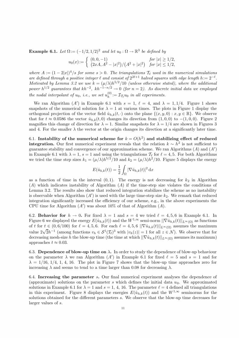
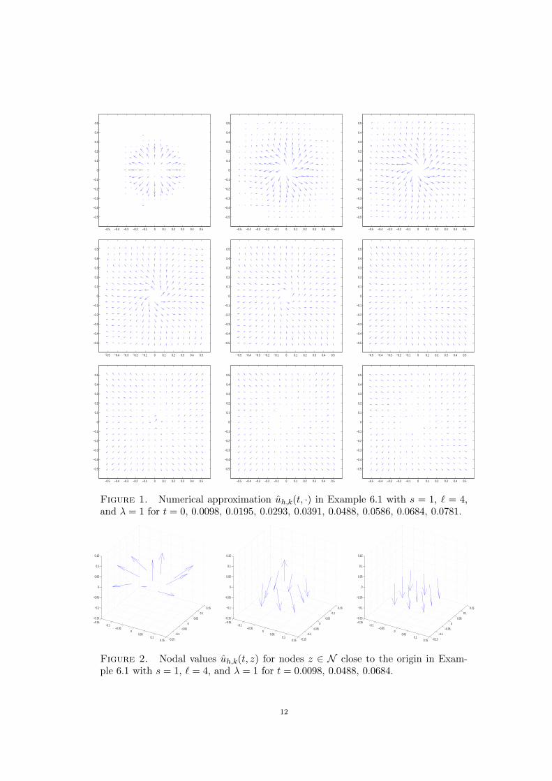
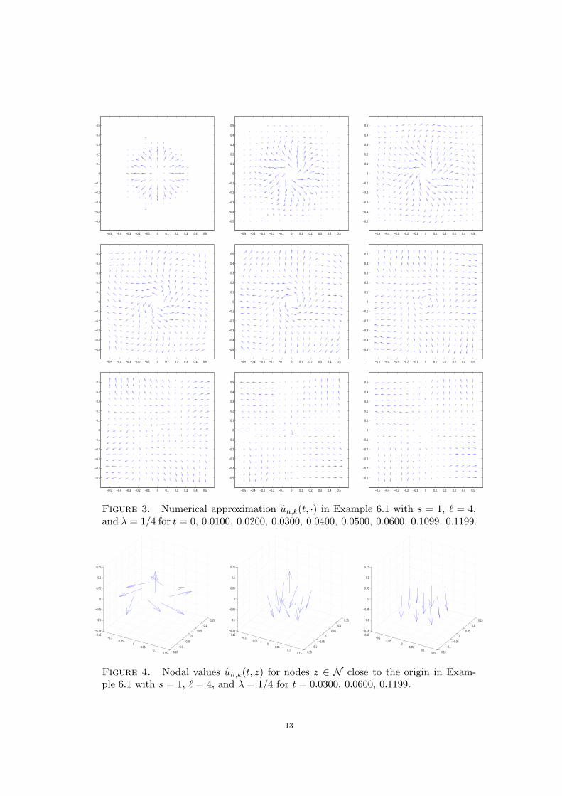
We ran Algorithm (A′) in Example 6.1 with s = 1, ` = 4, and λ = 1, 1/4. Figure 1 showssnapshots of the numerical solution for λ = 1 at various times. The plots in Figure 1 display theorthogonal projection of the vector field uh,k(t, ·) onto the plane (x, y, 0) : x, y ∈ R. We observethat for t ≈ 0.0586 the vector uh,k(t, 0) changes its direction from (1, 0, 0) to −(1, 0, 0). Figure 2magnifies this change of direction for λ = 1. Similar snapshots for λ = 1/4 are shown in Figures 3and 4. For the smaller λ the vector at the origin changes its direction at a significantly later time.

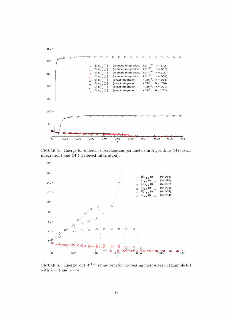
6.1. Instability of the numerical scheme for k = O(h2) and stabilizing effect of reduced

integration. Our first numerical experiment reveals that the relation k ∼ h2 is not sufficient toguarantee stability and convergence of our approximation scheme. We ran Algorithms (A) and (A ′)in Example 6.1 with λ = 1, s = 1 and using the triangulations T` for ` = 4, 5. For both Algorithmswe tried the time step sizes k1 = (µ/λ)h5/2/10 and k2 = (µ/λ)h2/10. Figure 5 displays the energy

E(uh,k(t)) =1

2

∫

Ω|∇uh,k(t)|2 dx

as a function of time in the interval (0, 1). The energy is not decreasing for k2 in Algorithm(A) which indicates instability of Algorithm (A) if the time-step size violates the conditions ofLemma 3.2. The results also show that reduced integration stabilizes the scheme as no instabilityis observable when Algorithm (A′) is used with the large time-step size k2. We remark that reducedintegration significantly increased the efficiency of our scheme, e.g., in the above experiments theCPU time for Algorithm (A′) was about 10% of that of Algorithm (A).

6.2. Behavior for h → 0. For fixed λ = 1 and s = 4 we tried ` = 4, 5, 6 in Example 6.1. InFigure 6 we displayed the energy E(uh,k(t)) and the W 1,∞ semi-norm ||∇uh,k(t)||L∞(Ω) as functionsof t for t ∈ (0, 6/100) for ` = 4, 5, 6. For each ` = 4, 5, 6 ||∇uh,k(t)||L∞(Ω) assumes the maximum

value 2√

2h−1 (among functions vh ∈ S1(T`)3 with |vh(z)| = 1 for all z ∈ N ). We observe that for

decreasing mesh-size h the blow-up time (the time at which ||∇uh,k(t)||L∞(Ω) assumes its maximum)approaches t ≈ 0.03.

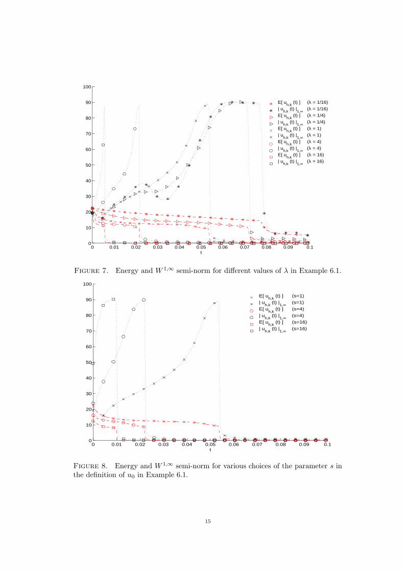
6.3. Dependence of blow-up time on λ. In order to study the dependence of blow-up behaviouron the parameter λ we ran Algorithm (A′) in Example 6.1 for fixed ` = 5 and s = 1 and forλ = 1/16, 1/4, 1, 4, 16. The plot in Figure 7 shows that the blow-up time approaches zero forincreasing λ and seems to tend to a time larger than 0.08 for decreasing λ.

6.4. Increasing the parameter s. Our final numerical experiment analyses the dependence of(approximate) solutions on the parameter s which defines the initial data u0. We approximatedsolutions in Example 6.1 for λ = 1 and s = 1, 4, 16. The parameter ` = 4 defined all triangulationsin this experiment. Figure 8 displays the energies E(uh,k(t)) and the W 1,∞ seminorms for thesolutions obtained for the different parameters s. We observe that the blow-up time decreases forlarger values of s.

11

−0.5 −0.4 −0.3 −0.2 −0.1 0 0.1 0.2 0.3 0.4 0.5

−0.5

−0.4

−0.3

−0.2

−0.1

0

0.1

0.2

0.3

0.4

0.5

−0.5 −0.4 −0.3 −0.2 −0.1 0 0.1 0.2 0.3 0.4 0.5

−0.5

−0.4

−0.3

−0.2

−0.1

0

0.1

0.2

0.3

0.4

0.5

−0.5 −0.4 −0.3 −0.2 −0.1 0 0.1 0.2 0.3 0.4 0.5

−0.5

−0.4

−0.3

−0.2

−0.1

0

0.1

0.2

0.3

0.4

0.5

−0.5 −0.4 −0.3 −0.2 −0.1 0 0.1 0.2 0.3 0.4 0.5

−0.5

−0.4

−0.3

−0.2

−0.1

0

0.1

0.2

0.3

0.4

0.5

−0.5 −0.4 −0.3 −0.2 −0.1 0 0.1 0.2 0.3 0.4 0.5

−0.5

−0.4

−0.3

−0.2

−0.1

0

0.1

0.2

0.3

0.4

0.5

−0.5 −0.4 −0.3 −0.2 −0.1 0 0.1 0.2 0.3 0.4 0.5

−0.5

−0.4

−0.3

−0.2

−0.1

0

0.1

0.2

0.3

0.4

0.5

−0.5 −0.4 −0.3 −0.2 −0.1 0 0.1 0.2 0.3 0.4 0.5

−0.5

−0.4

−0.3

−0.2

−0.1

0

0.1

0.2

0.3

0.4

0.5

−0.5 −0.4 −0.3 −0.2 −0.1 0 0.1 0.2 0.3 0.4 0.5

−0.5

−0.4

−0.3

−0.2

−0.1

0

0.1

0.2

0.3

0.4

0.5

−0.5 −0.4 −0.3 −0.2 −0.1 0 0.1 0.2 0.3 0.4 0.5

−0.5

−0.4

−0.3

−0.2

−0.1

0

0.1

0.2

0.3

0.4

0.5

Figure 1. Numerical approximation uh,k(t, ·) in Example 6.1 with s = 1, ` = 4,and λ = 1 for t = 0, 0.0098, 0.0195, 0.0293, 0.0391, 0.0488, 0.0586, 0.0684, 0.0781.

−0.15−0.1

−0.050

0.050.1

0.15 −0.15

−0.1

−0.05

0

0.05

0.1

0.15

−0.15

−0.1

−0.05

0

0.05

0.1

0.15

−0.15−0.1

−0.050

0.050.1

0.15 −0.15

−0.1

−0.05

0

0.05

0.1

0.15

−0.15

−0.1

−0.05

0

0.05

0.1

0.15

−0.15−0.1

−0.050

0.050.1

0.15 −0.15

−0.1

−0.05

0

0.05

0.1

0.15

−0.15

−0.1

−0.05

0

0.05

0.1

0.15

Figure 2. Nodal values uh,k(t, z) for nodes z ∈ N close to the origin in Exam-ple 6.1 with s = 1, ` = 4, and λ = 1 for t = 0.0098, 0.0488, 0.0684.

12

−0.5 −0.4 −0.3 −0.2 −0.1 0 0.1 0.2 0.3 0.4 0.5

−0.5

−0.4

−0.3

−0.2

−0.1

0

0.1

0.2

0.3

0.4

0.5

−0.5 −0.4 −0.3 −0.2 −0.1 0 0.1 0.2 0.3 0.4 0.5

−0.5

−0.4

−0.3

−0.2

−0.1

0

0.1

0.2

0.3

0.4

0.5

−0.5 −0.4 −0.3 −0.2 −0.1 0 0.1 0.2 0.3 0.4 0.5

−0.5

−0.4

−0.3

−0.2

−0.1

0

0.1

0.2

0.3

0.4

0.5

−0.5 −0.4 −0.3 −0.2 −0.1 0 0.1 0.2 0.3 0.4 0.5

−0.5

−0.4

−0.3

−0.2

−0.1

0

0.1

0.2

0.3

0.4

0.5

−0.5 −0.4 −0.3 −0.2 −0.1 0 0.1 0.2 0.3 0.4 0.5

−0.5

−0.4

−0.3

−0.2

−0.1

0

0.1

0.2

0.3

0.4

0.5

−0.5 −0.4 −0.3 −0.2 −0.1 0 0.1 0.2 0.3 0.4 0.5

−0.5

−0.4

−0.3

−0.2

−0.1

0

0.1

0.2

0.3

0.4

0.5

−0.5 −0.4 −0.3 −0.2 −0.1 0 0.1 0.2 0.3 0.4 0.5

−0.5

−0.4

−0.3

−0.2

−0.1

0

0.1

0.2

0.3

0.4

0.5

−0.5 −0.4 −0.3 −0.2 −0.1 0 0.1 0.2 0.3 0.4 0.5

−0.5

−0.4

−0.3

−0.2

−0.1

0

0.1

0.2

0.3

0.4

0.5

−0.5 −0.4 −0.3 −0.2 −0.1 0 0.1 0.2 0.3 0.4 0.5

−0.5

−0.4

−0.3

−0.2

−0.1

0

0.1

0.2

0.3

0.4

0.5

Figure 3. Numerical approximation uh,k(t, ·) in Example 6.1 with s = 1, ` = 4,and λ = 1/4 for t = 0, 0.0100, 0.0200, 0.0300, 0.0400, 0.0500, 0.0600, 0.1099, 0.1199.

−0.15−0.1

−0.050

0.050.1

0.15 −0.15

−0.1

−0.05

0

0.05

0.1

0.15

−0.15

−0.1

−0.05

0

0.05

0.1

0.15

−0.15−0.1

−0.050

0.050.1

0.15 −0.15

−0.1

−0.05

0

0.05

0.1

0.15

−0.15

−0.1

−0.05

0

0.05

0.1

0.15

−0.15−0.1

−0.050

0.050.1

0.15 −0.15

−0.1

−0.05

0

0.05

0.1

0.15

−0.15

−0.1

−0.05

0

0.05

0.1

0.15

Figure 4. Nodal values uh,k(t, z) for nodes z ∈ N close to the origin in Exam-ple 6.1 with s = 1, ` = 4, and λ = 1/4 for t = 0.0300, 0.0600, 0.1199.

13

0 0.01 0.02 0.03 0.04 0.05 0.06 0.07 0.08 0.09 0.10

50

100

150

200

250

300

350

t

E[ uh,k

(t) ] (reduced integration, k ∼ h2.5, h = 1/16)E[ u

h,k (t) ] (reduced integration, k ∼ h2, h = 1/16)

E[ uh,k

(t) ] (reduced integration, k ∼ h2.5, h = 1/32)E[ u

h,k (t) ] (reduced integration, k ∼ h2, h = 1/32)

E[ uh,k

(t) ] (exact integration, k ∼ h2.5, h = 1/16)E[ u

h,k (t) ] (exact integration, k ∼ h2, h = 1/16)

E[ uh,k

(t) ] (exact integration, k ∼ h2.5, h = 1/32)E[ u

h,k (t) ] (exact integration, k ∼ h2, h = 1/32)

Figure 5. Energy for different discretization parameters in Algorithms (A) (exactintegration) and (A′) (reduced integration).

0 0.01 0.02 0.03 0.04 0.05 0.060

20

40

60

80

100

120

140

160

180

t

E[ uh,k

(t) ] (h=1/16)

| uh,k

(t) |1,∞ (h=1/16)

E[ uh,k

(t) ] (h=1/32)

| uh,k

(t) |1,∞ (h=1/32)

E[ uh,k

(t) ] (h=1/64)

| uh,k

(t) |1,∞ (h=1/64)

Figure 6. Energy and W 1,∞ semi-norm for decreasing mesh-sizes in Example 6.1with λ = 1 and s = 4.

14

0 0.01 0.02 0.03 0.04 0.05 0.06 0.07 0.08 0.09 0.10

10

20

30

40

50

60

70

80

90

100

t

E[ uh,k

(t) ] (λ = 1/16)

| uh,k

(t) |1,∞ (λ = 1/16)

E[ uh,k

(t) ] (λ = 1/4)

| uh,k

(t) |1,∞ (λ = 1/4)

E[ uh,k

(t) ] (λ = 1)

| uh,k

(t) |1,∞ (λ = 1)

E[ uh,k

(t) ] (λ = 4)

| uh,k

(t) |1,∞ (λ = 4)

E[ uh,k

(t) ] (λ = 16)

| uh,k

(t) |1,∞ (λ = 16)

Figure 7. Energy and W 1,∞ semi-norm for different values of λ in Example 6.1.

0 0.01 0.02 0.03 0.04 0.05 0.06 0.07 0.08 0.09 0.10

10

20

30

40

50

60

70

80

90

100

t

E[ uh,k

(t) ] (s=1)

| uh,k

(t) |1,∞ (s=1)

E[ uh,k

(t) ] (s=4)

| uh,k

(t) |1,∞ (s=4)

E[ uh,k

(t) ] (s=16)

| uh,k

(t) |1,∞ (s=16)

Figure 8. Energy and W 1,∞ semi-norm for various choices of the parameter s inthe definition of u0 in Example 6.1.

15

Acknowledgment: Part of the work was written when S.B. visited ‘Forschungsinstitut furMathematik’ (ETH Zurich) in January 2005 and Brown University in March 2005. S.B. gratefullyacknowledges hospitality by the Department of Mathematics of the University of Maryland atCollege Park.

References

[1] Francois Alouges and Pascal Jaisson. Convergence of a finite elements discretization for the Landau-Lifshitzequations. preprint, 2003.

[2] Francois Alouges and Alain Soyeur. On global weak solutions for Landau-Lifshitz equations: existence andnonuniqueness. Nonlinear Anal., 18(11):1071–1084, 1992.

[3] John W. Barrett, Soren Bartels, Xiaobing Feng, and Andreas Prohl. A convergent and constraint-preservingfinite finite element method for the p-harmonic flow into spheres. (manuscript).

[4] Kung-Ching Chang, Wei Yue Ding, and Rugang Ye. Finite-time blow-up of the heat flow of harmonic maps fromsurfaces. J. Differential Geom., 36(2):507–515, 1992.

[5] Jean-Michel Coron. Nonuniqueness for the heat flow of harmonic maps. Ann. Inst. H. Poincare Anal. NonLineaire, 7(4):335–344, 1990.

[6] Boling Guo and Min-Chun Hong. The Landau-Lifshitz equation of the ferromagnetic spin chain and harmonicmaps. Calc. Var. Partial Differential Equations, 1(1):311–334, 1993.

[7] Stephen Gustafson, Kyungkeun Kang, and Tai-Peng Tsai. Schrodinger flow near harmonic maps. in preparation,2005.

[8] Joy Ko. The construction of a partially regular solution to the landau-lifshitz-gilbert equation in R2. preprint,

2005.[9] Martin Kruzık and Andreas Prohl. Recent developments in modeling, analysis, and numerics of ferromagnetism.

SIAM Review (accepted), also downloadable at: http://www.fim.math.ethz.ch/preprints/index.[10] Christof Melcher. Existence of partially regular solutions for Landau-Lifshitz equations in R

3. to appear in Comm.PDE.

[11] Francesca Pistella and Vanda Valente. Numerical study of the appearance of singularities in ferromagnets. Adv.Math. Sci. Appl., 12(2):803–816, 2002.

[12] Jalal Shatah and Chongchun Zeng. preprint. 2003.[13] Michael Struwe. On the evolution of harmonic mappings of Riemannian surfaces. Comment. Math. Helv.,

60(4):558–581, 1985.

Department of Mathematics, Humboldt-Universitat zu Berlin, Unter den Linden 6, D-10099 Berlin,

Germany

E-mail address: sba@math.hu-berlin.de

Department of Mathematics, Brown University, Providence, RI 02912, USA.

E-mail address: joyko@math.brown.edu

Department of Mathematics, ETH, CH-8092 Zurich, Switzerland.

E-mail address: apr@math.ethz.ch

16